Polvtechnic ' lnsfitute

USING TOURNAMENT TREES TO SORT

ALEXANDER STEPANOV AND AARON KERSHENBAUM

Polytechnic University 333 Jay Street Brooklyn, New York 11201

Center for Advanced Technology In Telecommunications

C.A.T.T. Technical Report 86- 13

CENTER FOR

ADVANCED

TECHNOLOGY IN

TELECOMMUNICATIONS

Using Tournament Trees to Sort

Alexander Stepanov and Aaron Kershenbaum

Polytechnic University 333 Jay Street

Brooklyn, New York 11201

stract

We develop a new data structure, called a tournament tree, which is a generalization of binomial trees of Brown and Vuillemin and show that it can be used to efficiently implement a family of sorting algorithms in a uniform way. Some of these algorithms are similar to already known ones; others are original and have a unique set of properties. Complexity bounds on many of these algorithms are derived and some previously unknown facts about sets of comparisons performed by different sorting algorithms are shown.

Sorting, and the data structures used for sorting, is one of the most extensively studied areas in computer science. Knuth [I] is an encyclopedic compendium of sorting techniques. Recent surveys have also been given by Sedgewick [2] and Gonnet [ 3 ] .

The use of trees for sorting is well established. Floyd's original Treesort 183 was refined by Williams 193 to produce Heapsort. Both of these algorithms have the useful property that a partial sort can also be done efficiently: i.e., it is possible to obtain the k smallest of N elements in O[N+k*log(N)] steps. (Throughout this paper, we will use base 2 logarithms.) Recently, Brown [6] and Vuillemin [7] have developed a sorting algorithm using binomial queues, which are conceptually similar to tournament queues, but considerably more difficult to implement.

The tournament tree data structure which we present allows us to develop an entire family of sorting algorithms with this property. The algorithms are all built around the same algorithmic primitives and therefore are all implemented with almost identical code which is concise, straightforward, and efficient. By selecting the appropriate mix sf primitives, we can implement sorts with excellent worst case performance, average case performance, or performance for specific types of data (e.g., partially ordered data).

We implement these primitives and the algorithms based on

This research supported by the New York State Foundation for Science and Technology as part of its Centers for Advanced Technology Program.

them and then analyze the algorithms I . performance. In doing so, we discover important similarities among algorithms previously thought to be different. We also show that the new data structure results in an implementation which is both more straightforward and more efficient than those of algorithms with comparable properties.

11. Tournament Trees

We define a tournament tree as a tree with the following properties:

# .

1) It is rooted; L e e , the links in the tree are directed from parents to children and there is a unique element with no parent.

2) The parent of a node has a key value which is less than or equal to that of the node. In general any comparison operator can be used as long as the relative values of parent and child are invariant throughout the tree. Thus, as in the case of a heap, the tree is a partial ordering of the keys. We will use the %81

operator throughout this paper and hence, refer to parents as %mallertf than their children in a heap.

As their name implies, tournament trees arise naturally in the course of competitions among the nodes, with the loser of a contest becoming the child of the winner. Figure 1 shows a tournament tree with 8 nodes. Trees with number of nodes not a power of 2 contain f1holesf8, which in general may be anywhere in the tree. We note that tournament trees are a proper generalization of heaps, which restrict a node to at most two children.

Figure 1: Tournament Trees

In addition to the above properties, we will sometimes find it useful to enforce the following additional properties:

3) The kth child of a node can itself have at most k children. We adhere to the convention that a node's children are indexed O,l,..k, starting from the right.

4) The root of a tree containing N nodes can have at most log(N) children.

These properties, which are maintained by some of the sorting algorithms presented below, allow us to guarantee worst case O[N log(N)] performance of the algorithms.

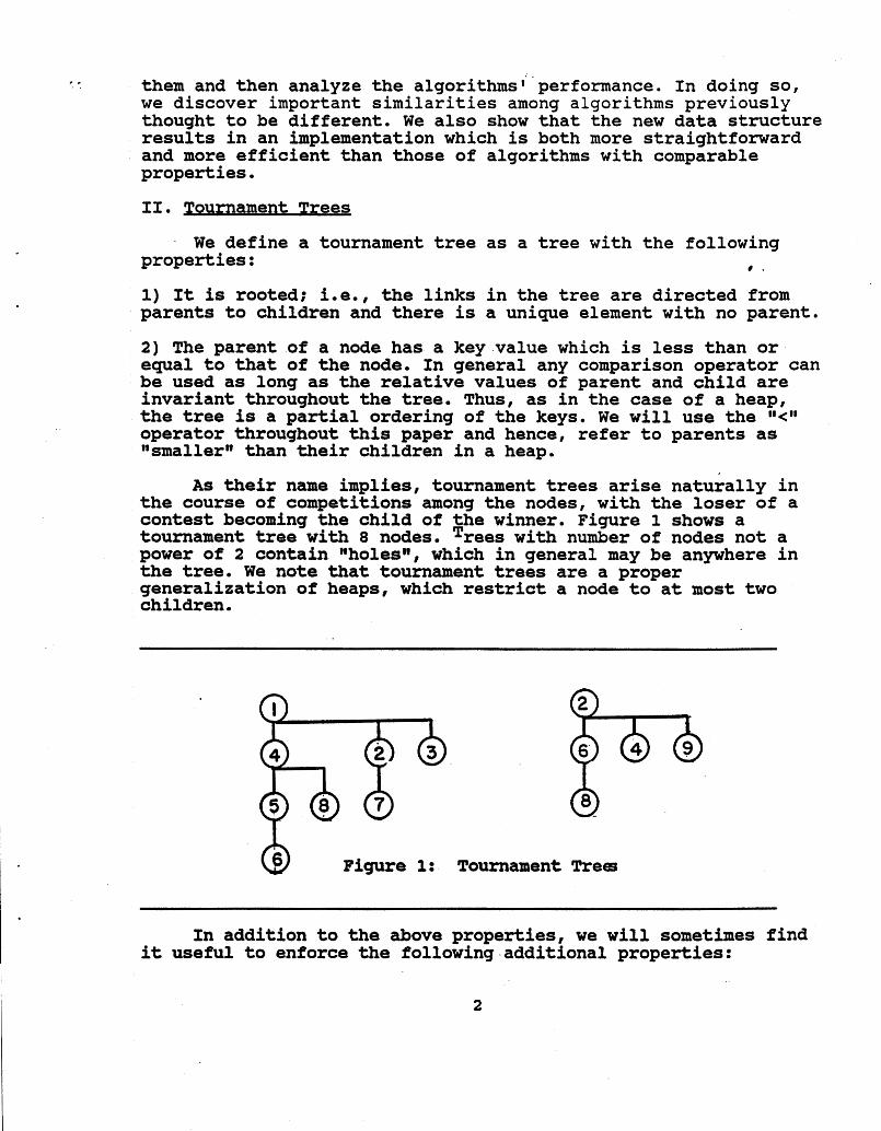
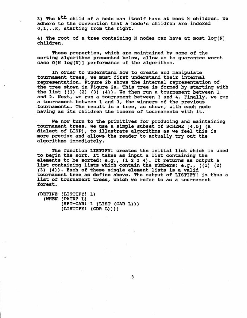
In order to understand how to create and manipulate tournament trees, we must first understand their internal representation. Figure 2b shows the internal representation of the tree shown in Figure 2a. This tree is formed by starting with the list ( (1) (2) (3) (4) ) . We then run a tournament between 1 and 2. Next, we run a tournament between 3 and 4. Finally, we run a tournament between 1 and 3, the winners of the previous tournaments. The result is a tree, as shown, with each node having as its children the losers of tournaments with it.

We now turn to the primitives for producing and maintaining tournament trees. We use a simple subset of SCHEME [4,5] (a dialect of LISP), to illustrate algorithms as we feel this is more precise and allows the reader to actually try out the algorithms immediately.

The function LISTIFY! creates the initial list which is used to begin the sort. It takes as input a list containing the elements to be sorted; e.g., (1 2 3 4). It returns as output a list containing lists which contain the numbers; e.g., ((1) (2) (3) (4)). Each of these single element lists is a valid tournament tree as define above. The output of LISTIFY! is thus a list of tournament trees, which we refer to as a tournament forest.

(DEFINE (LISTIFY! L) (WHEN (PAIR? L)

(SET-CAR! L (LIST (CAR L) ) ) (LISTIFY! (CDR L) ) ) )

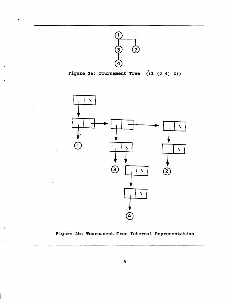
Figure 2a: Tournament Tree ((i ( 3 4 ) 2 ) )

Fig~re 2b: Tournament Tree Internal Representation

The next primitive is GRAB!, which takes two arguments (which are tournament trees) and makes the second the leftmost child of the first. Note that GRAB! does not create any additional CONS-cells (garbage) . (DEFINE (GRAB! X Y) (SET-CDR! Y (CDAR X) ) (SET-CDR! (CAR X) Y) X)

Figure 3 illustrates the operation of GRAB!. Using GRAB, it is simple to run a tournament between two nodes. The function TOURNAMENT-PLAY! takes as input the two tlplayerstl and a predicate indicating the type of competition which will be held: e.g., a comparison operator such as tt<tt or ti>tt. It plays the two competitors against one another and makes the loser the leftmost child of the winner. The arguments X and Y are tournament trees. The actual competitors are the values at the roots of these trees. We refer to these simply as the roots of the trees. GRAB! merges these two trees, creating a single tournament tree with the winner of the tournament as its root. Note that the way tournament trees are represented, the value at the root of a tournament tree is actually the CAAR (first element of the first element in the list) representing the tree.

Figure 3: Operation of GRAB!

(DEFINE (TOURNAMENT-PLAY! X Y PREDICATE) (IF (PREDICATE (CAAR X) (CAAR Y))

(GRAB! X Y) (GRAB! Y X) ) )

We define a tournament round to be a set of tournaments where the roots of pairs of trees in the tournament forest compete. The losers of each tournament are made children of the winners. Thus, a tournament round halves the number of trees in the forest. Note that TOURNAMENT-ROUND! forms the forest of winners in reverse order to their appearance in the original forest. This is done to avoid having to append one list to another; we have no actual preference for the order of the trees in the forest.

(DEFINE (TOURNAMENT-ROUND! SO-FAR TO-BE-DONE PREDICATE) (COND ( (NULL? TO-BE-DONE)

SO-FAR) ( (NULL? ( CDR TO-BE-DONE) (SET-CDR! TO-BE-DONE SO-FAR) TO-BE-DONE) (ELSE (LET ((NEXT (CDDR TO-BE-DONE))

(NEW (TOURNAMENT-PLAY! TO-BE-DONE (CDR TO-BE-DONE) PREDICATE) ) )

(SET-CDR! NEW SO-FAR) (TOURNAMENT-ROUND! NEW NEXT PREDICATE)))))

A tournament is defined as repeated tournament rounds which reduce a tournament forest to a forest containing a single tournament tree. The function TOURNAMENT! does this.

(DEFINE (TOURNAMENT! FOREST PREDICATE) (IF (NULL? (CDR FOREST) )

(CAR FOREST) (TOURNAMENT! (TOURNAMENT-ROUND! ' ( ) FOREST PREDICATE)

P-DICATE ) ) )

Thus, TOURNAMENT! is analogous to a function which sets up a heap at the beginning of Heapsort. Given N elements, it does a total of N-1 comparisons (as compared with 2N to set up a heap) and sets up a partial ordering among all the elements to be sorted. The root of the surviving tournament tree is the smallest element. We have thus determined the first element in the sorted

,.- list. We also know that the second element is one of the children of this element. This is reminiscent of the algorithm, given in Xnuth [I, pp. 209-2121 for determining the two smallest elements in a set using the minimum possible number of comparisons.

All we need to do to determine the next smallest element is

to run TOURNAMENT! on the children of .the root. Indeed, by repeating this step, we can complete the entire sort. The only other thing we need do is to accumulate the sorted elements. We thus have the following sorting algorithm.

(DEFINE (TOURNAMENT-SORT! PLIST PREDICATE) (LISTIFY! PLIST) (LET ( (P (TOURNAMENT! PLIST PREDICATE) ) ) (LET LOOP ( (X P) (NEXT (CDR P) ) ) (IF (NULL? NEXT)

P (LET ( (Y (TOURNAMENT! NEXT

PREDICATE) ) ) (SET-CDR! X Y) (LOOP y (CDR Y)))))))

Thus, TOURNAMENT-SORT! begins by converting the original list to a tournament forest. TOURNWNT! is then called to convert the forest to a single tournament tree with the smallest element as its root. Note that the value returned by TOURNAMENT! is the first element in the forest it works with: i.e., FOURNAMENT! returns the merged tournament tree which it creates. The root of this tree is the winner of the tournament; i.e., the [smallest remaining element in the tree. This smallest element is appended to the end of the list of sorted elements. The CDR (rest) of the list returned by TOURNAMENT! is again a tournament forest, suitable for passing to TOURNAMENT! to determine the next element in the sorted sequence. The procedure continues to call TOURNAMENT! to produce the next element in the sorted sequence until no elements remain to compete. When the procedure terminates, the original list has been sorted in place.

As an example of how TOURNAMENT-SORT! works, we consider sorting the list (2 5 1 4 3) . LISTIFY I converts the input to ( (2) (5) ( ) (4) (3) ) [Figure 4a]. TOURNAMENT! is called, which calls TOURNAMENT-ROUND!, which in turn calls TOURNAMENT-PLAY! with the arguments ( (2) (5) (1) (4) (3) ) , ( (5) (1) (4) (3) ) , and llO. The result of this call to TOURNAMENT-PLAY! is shown in Figure 4b. The value of SO-FAR is the tournament tree resulting from the comparisons of the roots of the first trees in each of the two forests passed to TOURNAMENT-PLAY! as arguments. TO-BE-DONE is a forest containing the remaining trees which have not yet participated in this tournament round.

Figure 4c shows the tournament forest at the end of the first tournament round. 2 and 5 have competed and 2 has won. 1 and 4 have competed and 1 has won. 3 has not competed and so remains as a root. As mentioned above, order of the trees in the forest has been reversed by TOURNAMENT-ROUND!.

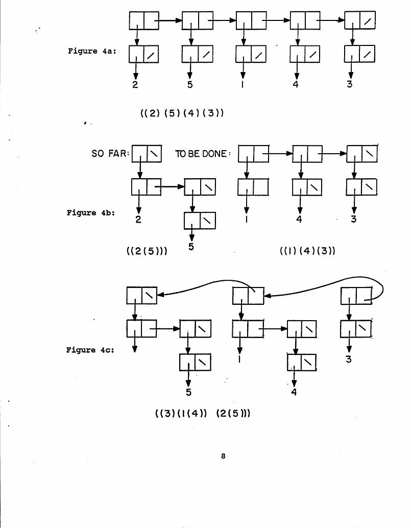
Figure 4c:

Figure

Figure 4e:

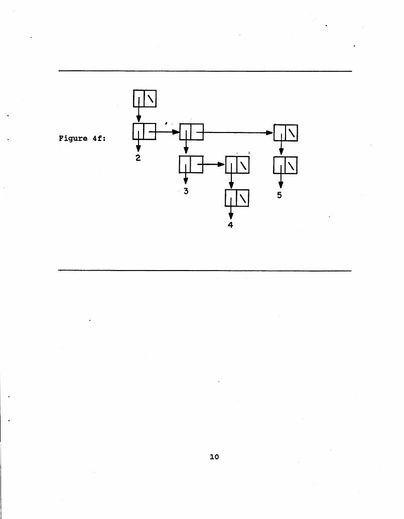
Figure 4f:

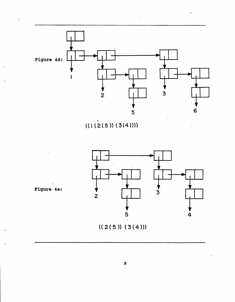
TOURNAMENT-ROUND! is called twice more to reduce the forest from 3 trees to 2 and then from 2 trees to 1. The resulting forest containing this one tree is shown in Figure 4d. At this point, the smallest element is the root (CAAR) of this tree and can be placed at the front of the list of sorted elements. The tournament forest can then be reduced one level (CDAR) leaving a new forest [Figure 4eJ whose tree roots are the children of the node just removed.

This forest is passed again to TOURNAMENT!. This makes the smallest remaining element the root of the single surviving tree. 'This tree is shown in Figure 4f. Again, the tree is reduced and TOURNAMENT! is called to find the next smallest element. It is instructive to examine the transformation from Figure 4e to Figure 4f as it is the result of a single GRAB! on two non- trivial trees, and hence, clearly illustrates how GRAB! works.

A Second Aluorithq

The above algorithm uses TOURNAMENT! to find the smallest remaining element, both at the beginning of the algorithm and during the remainder of it. TOURNAMENT! reduces a tournament forest to a single tree in adjacent elements. It does forest containing N trees.

a parallel fashion, comparing pairs of N-1 comparisons when initially fed a Thus, TOURNAMENT! can be thought of as

a parallel reduction operation.

Alternatively, we could use a sequential reduction operation to perform the tournament. Such an operation also does N-1 comparisons, but instead of working on successive pairs of elements, reducing the forest by half in each round, it sequentially plays the winner of each contest against the next tree in the list. The function SEQUENTIAL-TOURNAMENT! carries out this sequential reduction to set up the initial tournament tree.

(DEFINE (SEQUENTIAL-TOURNAMENT! FIRST SECOND PREDICATE) (IF (NULL? SECOND)

(CAR FIRST) (LEZ ((TWIRD (CDR SECOND)))

( SEQUENTIAL-TOURNAMENT ! (TOURNAMENT-PLAY ! FIRST THIRD PREDICATE) ) ) )

SEQUENTIAL-TOURNAMENT! plays

SECOND PREDICATE)

the first two trees in the list against one another, recording the identity of the third tree. It then plays the winner of this first contest against this recorded tree. As the SEQUENTIAL-TOURNAMENT proceeds, THIRD always points at the leftmost tree which has not yet participated in the tournament and FIRST points at the tree formed by the previous contest. As above, FIRST, SECOND, and THIRD are all actually tournament forests and the players are their leftmost trees. When mere is only one tree left in the forest, the tournament is over and returns the winning tree (CAR of the forest).

The original sort can then be easily modified to use BEQUENTIAL-TOURNAMENT! in place of TOURNAMENT! to find the second land remaining smallest elements. Note that we still use ~OURNAMENT!, which sets up a more balanced tree, to create the pnitial tree. We will discuss below the nature of the trees meated by both types of tournament.

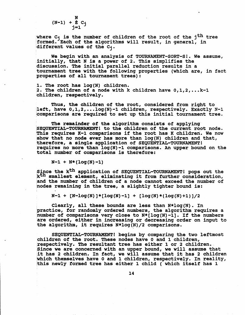
where Cj is the number of children of the root of the jth tree formed. Each of the algorithms will result, in general, in different values of the Cj.

We begin with an analysis of TOURNAMENT-SORT-S!. We assume, initially, that N is a power of 2. This simplifies the Idiscussion. The initial parallel reduction results in a tournament tree with the following properties (which are, in fact properties of all tournament trees) :

1. The root has log(N) children. 2. The children of a node with k children have 0,1,2,...k-1 children, respectively.

Thus, the children of the root, considered from right to left, have O,l,2,...log(N)-1 children, respectively. Exactly N-1 comparisons are required to set up this initial tournament tree.

The remainder of the algorithm consists of applying SEQUENTIAL-TOURNAMSNTI to the children of the current root node. This requires K-1 comparisons if the root has K children'. We now show that no node ever has more than log(N) children and Mat, therefore, a single application of SEQUENTIAL-TOURNAMENT! requires no more than log(N)-1 comparisons. An upper bound on the total number of comparisons is therefore:

N-1 + N* (log (N) -1) Si ce the kth application of SEQUENTIAL-TOURNAMENT! pops out the ktg smallest element, eliminating it from further consideration, and the number of children of a node cannot exceed the number of nodes remaining in the tree, a slightly tighter bound is:

Clearly, all these bounds are less than N*log(N). In practice, for randomly ordered numbers, the algorithm requires a number of comparisons very close to N*[log(N)-I]. If the numbers are ordered, either in increasing or decreasing order on input to the algorithm, it requires N*log(N)/2 comparisons.

SEQUENTIAL-TOURNAMENT! begins by comparing the two leftmost children of the root. These nodes have 0 and 1 children, respectively. The resultant tree has either 1 or 2 children. Since we are concerned with an upper bound, we will assume that it has 2 children. In fact, we will assume that it has 2 children iwhich themselves have 0 and 1 children, respectively. In reality, this newly formed tree has either 1 child ( which itself has 1

child) or two children (which both have no children). Thus, for the sake of simplifying the following discussion, we are assuming the existence of an additional node. This assumption cannot decrease the number of children of any node and hence cannot disturb the validity of any upper bound we find.

The next comparison is then between the newly formed tree and the third child of the root. Both nodes have 2 children and the resultant node has 3 children. Indeed, the newly formed node has 3 children which have 0,1 and 2 children, respectively. We have, in fact, replicated a tree of the same form as a subtree of the tree formed by TOURNAMENT! at the beginning of the procedure. Indeed, the kth comparison also compares the roots of 2 trees of this type, and forms another tree of this type. Finally, the last comparison in SEQUENTIAL-TOURNAMENT! forms a tree which is of exactly the same type as the tree formed by the original call to TOURNAMENT!, i.e., the root has exactly log(N) children which have O,l,...log(N) children, respectively. We have thus shown that no node ever has more than log(N) children and have thereby justified the upper bounds above.

A closer look at what is happening reveals that the initial tree formed by comparing the two leftmost children of the current lroot is in fact missing a node. The node that is lost is the root of the current tree, i.e., the kth smallest number which is

f opped out of the tree and removed from further consideration. his node is never replaced. Each successive application of EQUENTIAL-TOURNAMENT! removes another node from the tree. Some

pf these missing nodes are missing children of the current root and their absence results in the actual number of comparisons one in a given tournament being smaller than the upper bound.

when the numbers are ordered or nearly ordered on input o the algorithm, it becomes likely that the root is missing one r more children and the actual number comparisons is roughly

halved. We will see that this is in fact the best case for this lalgorithm.

We now show that when the element values are unique and N, the number of elements is a power of 2, that TOURNAMENT-SORT-S! does exactly the same comparisons as Mergesort, but in a somewhat pifferent order.

Consider the operation of Mergesort. It makes log(N) passes through the data. The kth pass merges lists of zkal numbers forming lists of 2k numbers. Thus, for example, if the inpu': to pergesort is 1, 2, 6, 3 , 8, 5, 7, 4, there are three passes producing the following lists:

During each pass, successive pairs of lists are merged. This comparing numbers of one list with numbers in the list

aired with it. Note, however, that not all pairs are compared. ome numbers are %hieldedv8 from comparison by other numbers. For

in the first pass, 3 shields 6 from comparison with 1, 1 is found to be less than 3 (by direct comparison)

, , known to be less than 6 (since the lists being merged

lare already sorted), 1 is never compared with 6. Similarly, 3 shields 6 from comparison with 2. In general, i shields j from comparison with k if i and j are members of the same list, i is less than j, k is a member of the other list, and i is greater khan k.

In the best case, the first number of one list in each pair is larger than all the numbers in the other list, shielding all e remaining numbers in its list from all the numbers in the ther list. This results in N/2 comparisons per pass and a total k Of N*log(N)/2 comparisons, when N is a power of 2. This situation bctually occurs if the numbers are ordered (in either increasing r decreasing order) on input to the sort. in the worst case,

2 lists of length k are merged, there are 2k-1 comparisons. of 2, this results in N*[log(N)-lJ+l case can also arise in practice for

ordered numbers and is a close approximation to comparisons which arise in practice when the sorted are randomly ordered on input.

We now consider the operation of TOURNAMENT-SORT-S!. Figure shows the trees formed for the same 8 numbers shown above. We irst note that the comparisons done by Reduction Sort are in fact the same as those done by Mergesort. There are 15

R omparisons: 12, 36, 58, 47, 13, 45, 14, 23, 24, 34, 46, 57, 56, 8, and 67. The first 7 are to set up the original tree. The next p make 2 the root of the following tree. The next one makes 3 the poot of the following tree, etc. Looking again at Mergesort, we find it does the comparisons 12, 36, 58, and 47 on the first

1 ass, the comparisons 13, 23, 45, 57, and 78 on the second pass, nd the comparisons 14, 24, 34, 46, 56, and 67 on the third pass c the same 15 comparisonsl

This is not a coincidence. Looking clo:~ely, we see that the 4 comparisons done by both sorts are the same; they are

omparisons of successive pairs of numbers in the original list. he remaining comparisons done by TOURNAMENT-SORT-S! in setting p the initial tree correspond exactly to the first comparisons one in merging pairs of lists in Mergesort. The nested subtrees

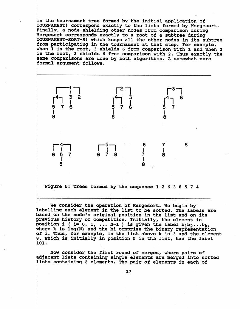
in the tournament tree formed by the initial application of TOURNAMENT! correspond exactly to the lists formed by Mergesort. Finally, a node shielding other nodes from comparison during Mergesort corresponds exactly to a root of a subtree during TOURNAMENT-SORT-S! which keeps all the other nodes in its subtree from participating in the tournament at that step. For example, when 1 is the root, 3 shields 6 from comparison with 1 and when 2 is the root, 3 shields 6 from comparison with 2. Thus exactly the same comparisons are done by both algorithms. A somewhat more formal argument follows.

Figure 5: Trees formed by the sequence 1 2 6 3 8 5 7 4

We consider the operation of Mergesort. We begin by labelling each element in the list to be sorted. The labels are based on the node's original position in the list and on its

of competition. Initially, the element in N-1 ) is given the label blb2.. .bk! bi comprise the binary representatlon in the list above k is 3 and the element position 5 in the list, has the label

I Now consider the first round of merges, where pairs of adjacent lists containing single elements are merged into sorted lists containing 2 elements. The pair of elements in each of

ithese initial merges have the labels blb2. . . bk and blb2. . . bk r

where we use bk to denote 1-bk. We relabel the winner of the /competition blb2.. .bk-l*. We use *Is in the rightmost positions of a label to indicate that an element has won competitions. A label with *Is in the rightmost j positions indicates the element has won a competition in the jth round.

In the general case (after the first round) we would then Fliminate the,winner of each of these competitions from further lconsideration in this round and continue the merge of each pair of lists. In the first round, however, this is a trivial operation. The one element in the list containinqthe winner has b een eliminated and so there is no element for the loser of each P revious competition to compete with. The previous loser therefore wins its next competition in this round by default and receives a label of blb2. . . bk-l*.

elements. We consider are merged. The leftmost

have labels respectively. (j * e) and is

ompetition with the next element in the list containing the revious winner. We note that all the elements remaining in each ist have the same labels and that therefore the two competitors ave the same labels as those in the previous competition. (Since 11 the elements in a list have the same label, we will sometimes efer to the list itself by this label. We can Thus speak of a erge between lists blb 2...bj*e..* and blb 2...b **...*.) Again, e relabel the winner and eleminate it from furtier consideration

En this round. We continue this merge until there are no elements remaining in one of the lists. All the elements remaining in the pther list then have no one to compete with and they win their emaining competitions in this round by default, receiving a new abel as if they had won an actual competition.

All that we have been describing is the ordinary operation f the merging of two ordered lists. gy keeping track of the lement labels, however, we are able to see more precisely which ements are competing. In particular, we note that in round j at elements compete with other elements whose labels match eir own except in the k+l-jth position. More specifically, an ement, i, with value vi, competes with all elements in its mate st (i.e., the list of elements, m, with labels matching its own cept in position k+l-j) with values in the range

where element p precedes element i in its current list. We see this is true because any element, m, with v, < vp would have already won in this round and have been eliminated from further competition before competing with i. All elements m in the above range will compete with i and win. i will compete once more with an element q which is the next element in the mate list after the last m that i competes with; i.e., the smallest v such that vq > vi. i will win this competition and not compete fzrther in this 1 round.

The above operations continue until finally in the kth round a single sorted list of N elements is formed. All the winners at this level receive labels of **...*, indicating they are the smallest remaining elements.

We now consider the operation of TOURNAMENT-SORT-S!. We label the elements in exactly the same way as we did in Mergesort above and will see by considering the labels of the competing elements, that exactly the same elements are compared as were before, although the comparisons are done in a somewhat different order.

The initial round of SEQUEWTIAL-TOURNAMENT! is identical to the initial round of merges. The same nodes are comparea and they receive the sane labels. Succeeding rounds of SEQUENTIAL- TOURNAMENT! correspond to the first competitions in each of the merges done by Mergesort, i.e., the smallest (leftmost) pair of elements with labels blb 3...b *...* and blb compared and the winner is gi en the label b Unlike in Mergesort, however, these merges completion; only the first competition, determining the smallest element in each list, is carried out.

Looking at the tree in Figure 6, we observe that the root as the label ***. This must be the case since it has competed at 11 levels and won all competitions. This element is the smallest f all and is ready to leave the entire tournament as the first lament in the sorted list. The elements it competed with are the urrent heads (smallest elements) of the appropriate mated lists; i.e., if the root originally had the label blb2...bk, then it

I Figure 6 shows the initial tournament tree produced by SEQUENTIAL-TOURNAMENT! along with the labels on each node at this point. Note that, unlike in Mergesort, each element has a unique label.-All elements acquire exactly the same labels in both algorithms, but they do so at different times because of the different order of competitions. In fact, it is clear that the only labels a node can acquire are its original label, which is unique to its position in the original list (and is the same in both algorithms) and this same labels with more and more of the rightmost positions filled with *Is. Thus, it is clear that elements acquire the same labels in both algorithms.

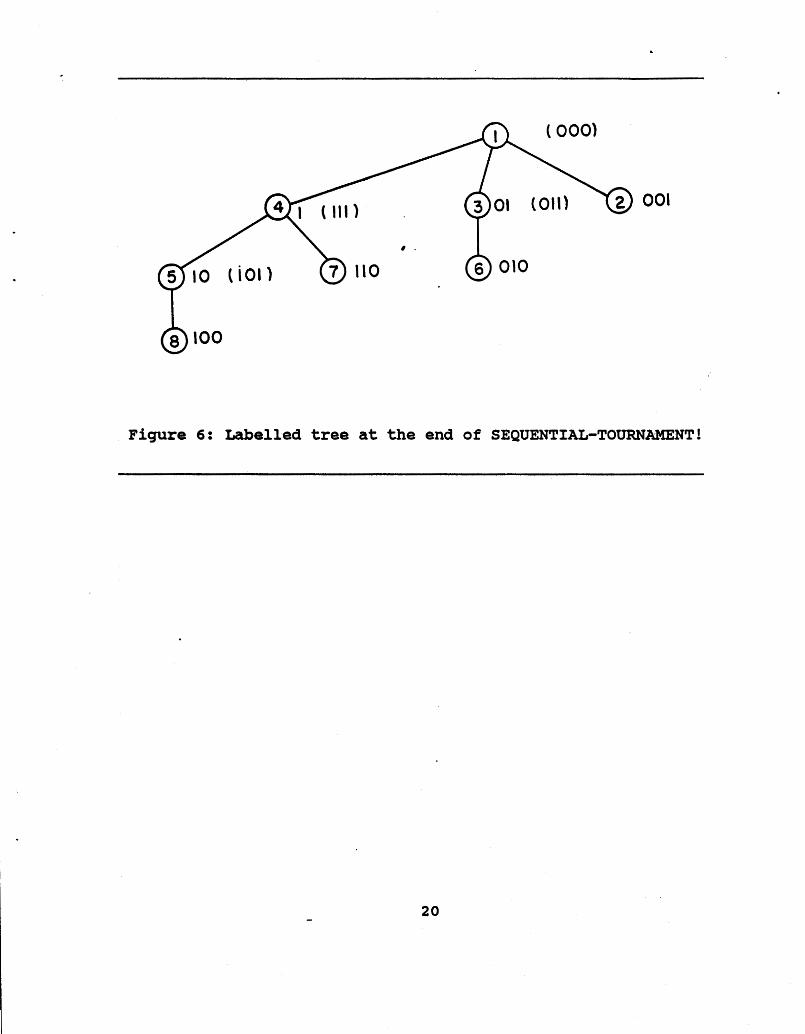
Figure 6: Labelled tree at the end of SEQUENTIAL-TOURNAMENT!

I I cympeted with the heads of lists blb 2...b k, blb 2...b kT1*, ... b 1*...* . As we will see, SEQUENTIAL-TOURNAMENT! maintams this property and the root will always compete with heads of lists of this form. Since the root wins all these competitions, the losers become its children from right to left. Thus, the children of the root after the application of SEQUENTIAL-TOURNAMENT! will have the same types of labels as they did before the application of SEQUENTIAL-TOURNAEJIENT!. Afterwards, however, elements will have labels with bit patterns relative to the new root rather than the old one. The only other change, as we shall see, is that one node in the tree (corresponding to the root just removed) will be missing. Thus, the new tree will have a llholell.

Continuing with the operation of TOURNAMENT-SORT-S!, we call SEQUENTIAL-TOURNAMENT! to find the next smallest element. This amounts to playing the children of the root against one another from right to left. In the actual coding of SEQUENTIAL- TOURNAMENT!, it is convenient to play the children from left to right. We need to play them from right to left, however, to maintain this useful property of self replication. We therefore reverse the list of children before calling SEQUENTIAL- TOURN-! .

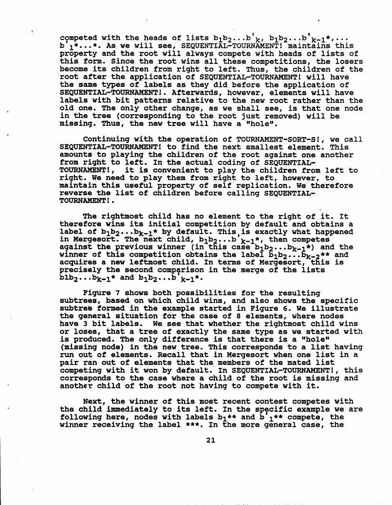
The rightmost child has no element to the right of it. It therefore wins its initial competition by default and obtains a label of blb2...bk-l* by default. ThisIis exactly what happened in Mergesort. The next child, blb 2...b k-I*, then competes against the previous winner (in this case blb2...bk-l*) and the winner of this competition obtains the label blb2...bk-2** and acquires a new leftmost child. In terms of Mergesort, this is precbely the second comp~rison in the merge of the lists blb 2...bk,l* and blb 2...b k-I*.

Figure 7 shows both possibilities for the resulting subtreas, based on which child wins, and also shows the specific subtree formed in the example started in Figure 6. We illustrate the general situation for the case of 8 elements, where nodes have 3 bit labels. We see that whether the rightmost child wins or loses, that a tree of exactly the same type as we started with is produced. The only difference is that there is a (missing node) in the new tree. This corresponds to a list having run out of elements. Recall that in Mergesort when one list in a pair ran out of elements that the. members of the mated list competing with it won by default. In SEQUENTIAL-TOUIWAMENT!, this corresponds to the case where a child of the root is missing and another child of the root not having to compete with it.

Next, the winner of this most recent contest competes with the child immediately to.its left. In the spvcific example we are following here, nodes with labels bl** and b I** compete, the winner receiving the label ***. In the more general case, the

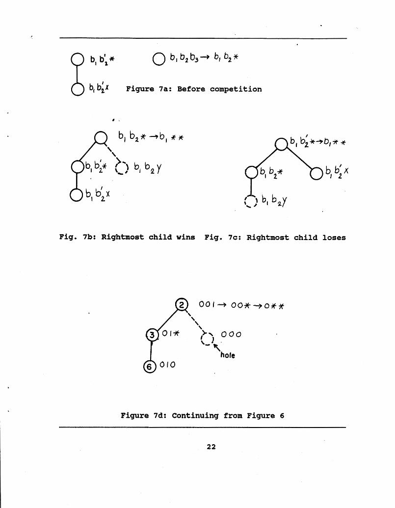
Figure 7a: Before competition

Fig. 7b: Rightmost child wins Fig. 7c: Rightmost child loses

Figure 7d: Continuing from Figure 6

cornpetitton would be between nodes blb2. . .b$-2** and bab 2...b %,2**. The loser becomes the new rightmost child of the winner. Flgure 8 illustrates the situation after the second (and final) comparison for the specific example we are following.

We observe that this tree is of exactly of the same form as the tree in Figure 6. Observing the operation of SEQUENTIAL- TOURNAMENT!, we see this is true in general. The only difference is that in general the hole may be in a different place. In this case, the hole corresponds to the list OO* having run out of elements giving 3 and 6, the elements in the list Ol* a "free riden in the remainder of their competition: this is exactly what happened in Mergesort.

Thus, this first application of SEQUENTIAL-TOURNAMENT! corresponds to comparisons in Mergesort. In particular, it corresponds exactly to the comparisons involving the lists containing element 1 right after element 1 was removed from competition at each level (We are referring to elements by their values, not their positions. It is a coincidence that the element with value 1 happened to be the first element in the original list.) Thus, since element 1 was the last (only) element in the 000 list, element 2 does not have to compete a the first, level. Element 3, the current smallest in the Ol* list, competes with element 2, the current smallest (after element 1 was eliminated) in the 001 list. Finally, element 4, the smallest in list I**, competes with 2, the smallest in O**.

Successive calls to SEQUENTIAL-TOURNAMENT! (with element r with label blbl...bk as the root) result in replicating this tree rstructure, which is in fact the tournament tree we have been talking about all along. Each successive tree contains a new hole corresponding to the newly removed root, as well as all the holes creates in previous rounds. The comparisons done are precisely - - those involving the lists blb2...bk, blb2...bk-l*,... and bl*...* at the'point right after element r was eliminated from these lists. 1f any 02 the lists was empty at that time, a hole will be there in place of the list and a comparison will be skipped.

Since every node becomes the root eventually and every comparison done by Mergesort can be considered at the point that some node has just been removed (except for the initial comparisons which we accounted foy in setting up the original tournament tree), we see that Mergesort and TOURNABENT-SORT-S! do exactly the same comparisons. The difference between the two sorts is that TOURNAMENT-SORT-SL does them in the order of the winning Phis is partial without

elements, always producing the next smallest element. in general a useful feature as it permits us to do sorts, obtaining the j smallest elements in a list totally sorting the list.

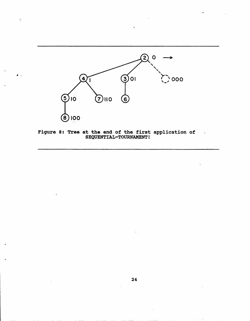
Figure 8: Tree at the end of the first application o f SEQUENTIAL-TOURNAHENT!

VII . In a manner very similar to that used above to demonstrate

the similarity between TOURNAMENT-SORT-S! and Mergesort, we show that the comparisons by TOURNAMENT-SORT-S! are identical to those done by the Floyd's Tournament Sort (83.

Floyd's sort begins by running competitions between adjacent pairs of elements. The winners of these first-round tournaments compete in the second round. Winners of succeeding rounds continue to compete until a single winner remains. This process is carried out using a vector twice the length of the original number of elements to be sorted.

The result of this initial round of competitions is shown in Figure 9a for the 8 element example we have been using to illustrate the performance of all the sorting algorithms. As above, in the discussion that follows we assume that N, the number of elements, is a power of 2 and all the element values are unique. In Figure 9, we have added labels to each of the elements. These labels are not part of Floyd's original algorithm and are not needed for its operation: they are present simply to facilitate this discussion.

The column labeled Position is part of Floyd's algorithm. It was implemented by packing it into the low order bits of the elements and was necessary for the proper performance of the algorithm. It is interesting to note that if these low order bits are included in the comparisons of element values, the values become unique and the sort becomes stable.

Examining Figure 9a, it is clear that all comparisons done during this first stage of Floyd's algorithm are betrean nodes with labels of the form blb 2...bj*...* and blb2 ... bj *...*, with the node receiving labels exactly as they did above. Thus, we see that the comparisons done in this initial phase are the same as the ones clone by TOURNAMENT-SORT-S!.

Floyd's algorithm next removes the winner of the first stage from further consideration and, based upon its position, which is carried along, redoes all the competitions involving this element. Depending upon the implementation, this may include "null" comparisons including removed elements. We do not count such comparisons here. In this case, therefore, the null comparison between 1 (which has been removed) and 2 is not considered; 2 is considered the winner by default and the label on 2 is changed to OO*. The competition between OO* and 01* (originally between 1 and 3, now between 2 and 3) is repeated, a's is the competition between 0** and 1** (originally between 1 and 4, now between 2 and 4). This is illustrated in Figure 9b. In general, we see that if the element whose original label was b1b2...bk wins the current round, then the comparisons involving

nodes with labels blb2...bk, blb2...bk-1*, blb2...bj*...*, ... bl*. . .* are redone. Furthermore, if the implementation involves maintaining something akin to the node labels we are using for illustration here, then null comparisons can be recognized by only repeating comparisons involving nodes with labels blb 2...b *...* through bl*.. .*, where the winner of the current d round ha label blb 2...bj*.*...* at the beginning of the current round. Thus, again, we see that the same comparisons are done as were done before by TOURNAMENT-SORT-S!. As this last step is repeated by Floyd's algorithm to successively produce all the remaining elements in sorted order, we see that the two algorithms do exactly the same comparisons (excluding the null comparisons which may possibly be done by Floyd's algorithm) in exactly the same order.

We note at this time that while Floyd's algorithm and TOURNAMENT-SORT-S! do the exactly the same comparisons, that they are not that same algorithm, any more than Mergesort and Floyd's algorithm are the same algorithm although Mergesort also does the same comparisons. The tournament tree structure used by TOURNAMENT-SORT-SI and the other sorts we present here gives rise to a much more flexible, and much more efficient, implementation. Computational experience has shown TOURNmNT-SORT-S! to be roughly twice as fast as Floyd's algorithm, as well as being able to handle lists, a more general data structure.

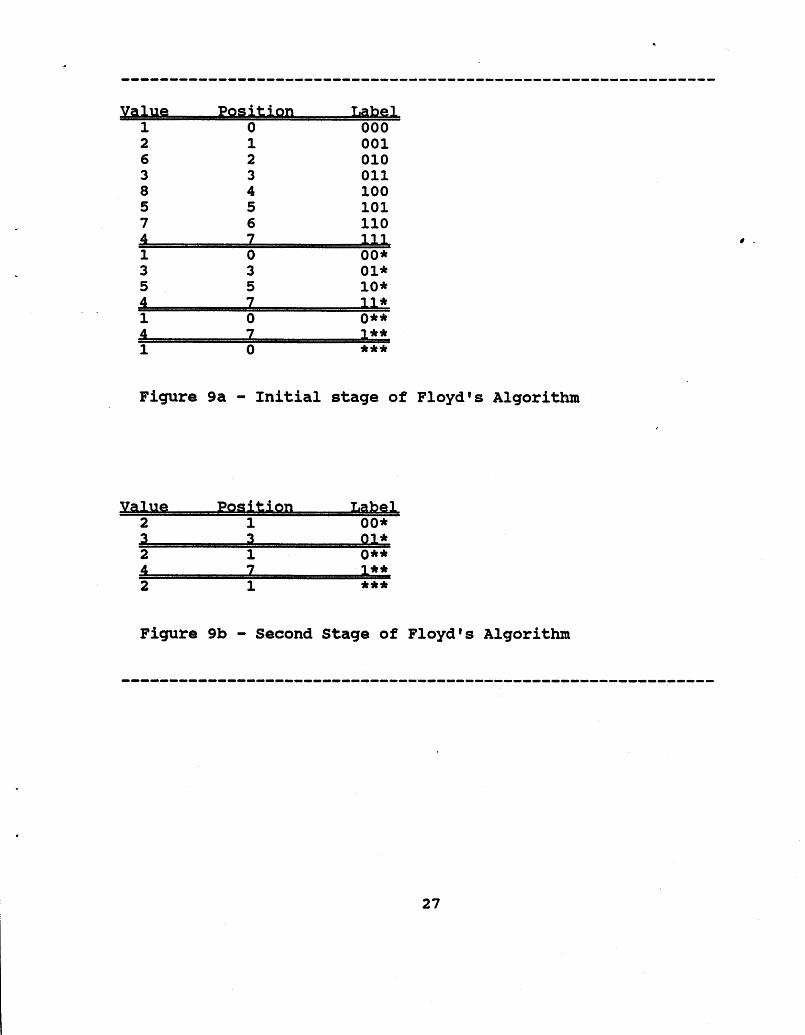
Figure 9a - Initial stage of Floyd's Algorithm

ue Poati-&&g& 2 1 OO*

Figure 9b - Second Stage of Floyd's Algorithm

VIII . We briefly described a modified version of TOURNAMENT-SORT-

S!, where SEQUENTIAL-TOURNAMENT! is used both to set up the original tournament tree and to pop out the remaining elements in sorted order. We refer to this sort as TOURNAMENT-SORT-S2!. We now show that a slightly modified version of TOURNAMENT-SORT-S2! does exactly the same comparisons as Insertion Sort, but in a different order which allows the former to function as a partial sort (like Selection Sort) where the latter does not. Thus, we will see that the same relationship exists between TOURNAMENT- SORT-S2! and Insertion Sort as exists between TOURNAMENT-SORT-S! and Mergesort.

. For the sake of this analysis, we reverse the order of the trees-in the tournament forest before calling SEQUENTIAL- TOURNAMENT!. The reversal makes TOURNAMENT-SORT-S2! identical to TOURNAHENT-SORT-S! except for the call to SEQUENTIAL-TOURNAMENT! ineplace of TOURN2WENTI. The reversal of the tree is not necessary in TOURNAMENT-SORT-S2!. As far as we can tell, it neither helps not hinders in terms of the number of comparisons done. Thus, in practice it is wasted effort and should not be done. We do it here only to illustrate the equivalence Of the comparisons done by TOURNAMENT-SORT-S2! and Insertion Sort.

Given a list of elements, Insertion Sort passes through the list from left to right and builds a sorted list of elements by inserting each element into the sorted list. This involves comparing each element in the original list with each element in the sorted list until a larger element is found in the sorted list. Having found the first larger element, the new element can be inserted before it in the sorted list. The Lemma below follows from this definition of Insertion Sort. Let v+ be the value of the element originally in position i in the list of elements to be sorted.

w: For i > j, Vi and WJ are compared iff Vi > Vj or if Vj is the smallest element larger than Vi (and for which 1 > j).

Now consider the operation of TOURNAMENT-SORT-S2!e We note that SEQUENTIAL-TOURNAMENT! does not disturb the relative order of the children of a node; L e e , if elements el, eq, ... ek are the children of a given node, in that order from rlght to left, then these elements appeared in the same order in the original list. This follows from the fact that the first application of SEQUENTIAL-TOURNAMENT! passes through the original list of elements from left to right and inserts children from right to left; thereafter, it passes through the children of a node from right to left (after the reversal of the trees in the tournament forest) and again inserts children from right to left.

We now observe that if Vi < vk < v * and i > k and i > j then by the above property of SEQUENTIAL-TO&AMENT! element j will become a child of element k before being compared with element i. Element j will remain a child of element k until element k is removed from further consideration, which is after element i is removed from consideration, since vj < vk. Thus elements vi and Vj are never compared. On the other hand, if no such vk exists, vj will not be the child of any other node when it comes time to compare it with Vi and the two elements will be compared. We thus see that the Lemma holds for TOURNAMENT-SORT-S2! as well and that both algorithms do the same comparisons. Figure 10 illustrates the operation of TOURNAMENT-SORT-SZ! for our example.

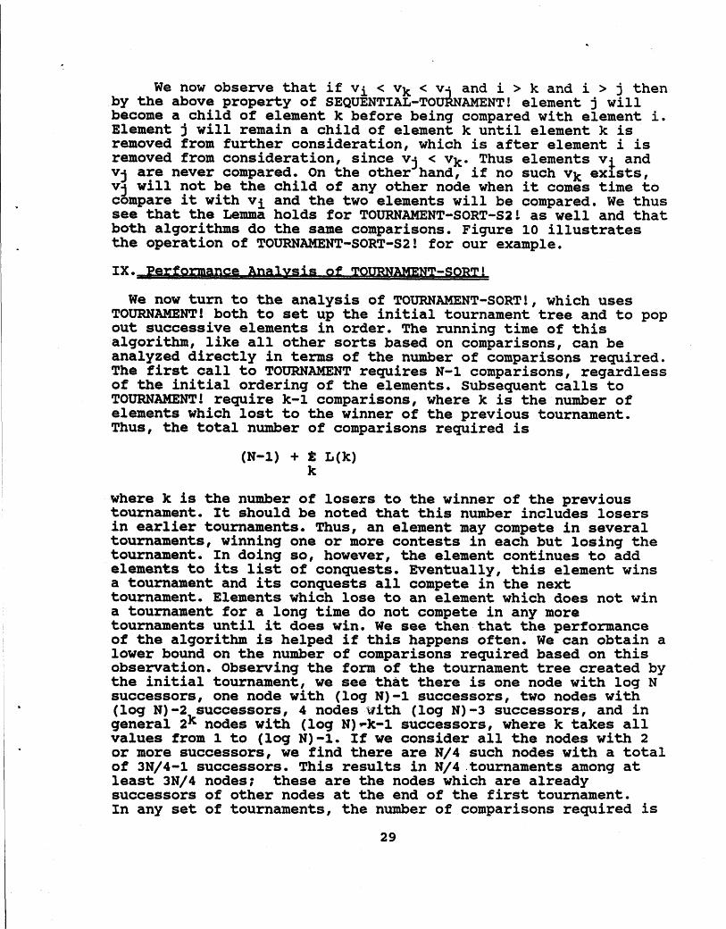
We now turn to the analysis of TOURNAMENT-SORT!, which uses TOURNAMENT! both to set up the initial tournament tree and to pop out successive elements in order. The running time of this algorithm, like all other sorts based on comparisons, can be analyzed directly in terms of the number of comparisons required. The first call to TOURNAMENT requires N-1 comparisons, regardless of the initial ordering of the elements. Subsequent calls to TOURNAMENT! require k-1 comparisons, where k is the number of elements which lost to the winner of the previous tournament. Thus, the total number of comparisons required is

where k is the number of losers to the winner of the previous tournament. It should be noted that this number includes losers in earlier tournaments. Thus, an element may compete in several tournaments, winning one or more contests in each but losing the tournament. In doing so, however, the element continues to add elements to its list of conquests. Eventually, this element wins a tournament and its conquests all compete in the next tournament. Elements which lose to an element which does not win a tournament for a long time do not compete in any more tournaments until it does win. We see then that the performance of the algorithm is helped if this happens often. We can obtain a lower bound on the number of comparisons required based on this observation. Observing the form of the tournament tree created by the initial tournament, we see that there is one node with log N successors, one node with (log N)-1 successors, two nodes with (log N) -2 successors, 4 nodes with (log N) -3 successors, and in general 2k nodes with (log N)-k-1 successors, where k takes all values from 1 to (log N)-1. If we consider all the nodes with 2 or more successors, we find there are N/4 such nodes with a total of 3N/4-1 successors. This results in N/4.tournaments among at least 3N/4 nodes; these are the nodes which are already successors of other nodes at the end of the first tournament. In any set of tournaments, the number of comparisons required is

Figure 10: TOURNaMENT-SORT-S2!

equal to the total number of nodes competing minus the number of tournaments. Thus, there will be N/2 comparisons in the N/4 tournaments among 3N/4 nodes. Based on this, there will be at least (3/2)N-2 comparisons in total. This is just a lower bound. In reality, a node can lose to the winner of the next tournament and compete again immediately. It is in fact possible in theory for one node to always lose to the winner of the next tournament and to compete in all N tournaments; it is not, however, possible for all nodes to be so unfortunate.

As mentioned above, it is best if nodes lose to other nodes which do not win a tournament for a long time. This is, remarkably, essentially what,happens when the elements are initially in order, or near y in order. If we look at a typical ?i situation where there are 2 elements to be sorted and these e ements are already in order (see Figure 11), we see that node zB1+l loses immediately to node 2k-2+1. It later loses to node 2k'2+2k-3+l, and so on, until it finally loses to node zk-l. Thus, it competes with log N nodes, losing to all of them. During the first N/2 tournaments none of the other last N/2 nodes compete at all because the root of the tree containing them lost all its competitions. We can therefore look at the process of sorting N elements as one of sorting the first N/2 elements followed by sorting the second N/2 elements, except for the presence of the element ~~'l+l (=N/2+1) in both sorts. Thus, c(N), the number of comparisons required in this case to sort N elements is given by:

c (N) = 2c (N/2) + f (N) where f(N) is a factor which accounts for the presence of element N/2+1 in the first part of the sort. We expect f(N) to look like log N, and it in fact does. Empirically, we observed f (N) by counting the number of comparisons required to so N already fZ sorted elements for values of N equal to 2k and 2 1. A brief table of these values is printed below. Also shown in the table are c(N), the number of comparisons required by TOURN-NT-SORT! when the inputs are sorted. As can be seen, c(N) is very close to 2N.

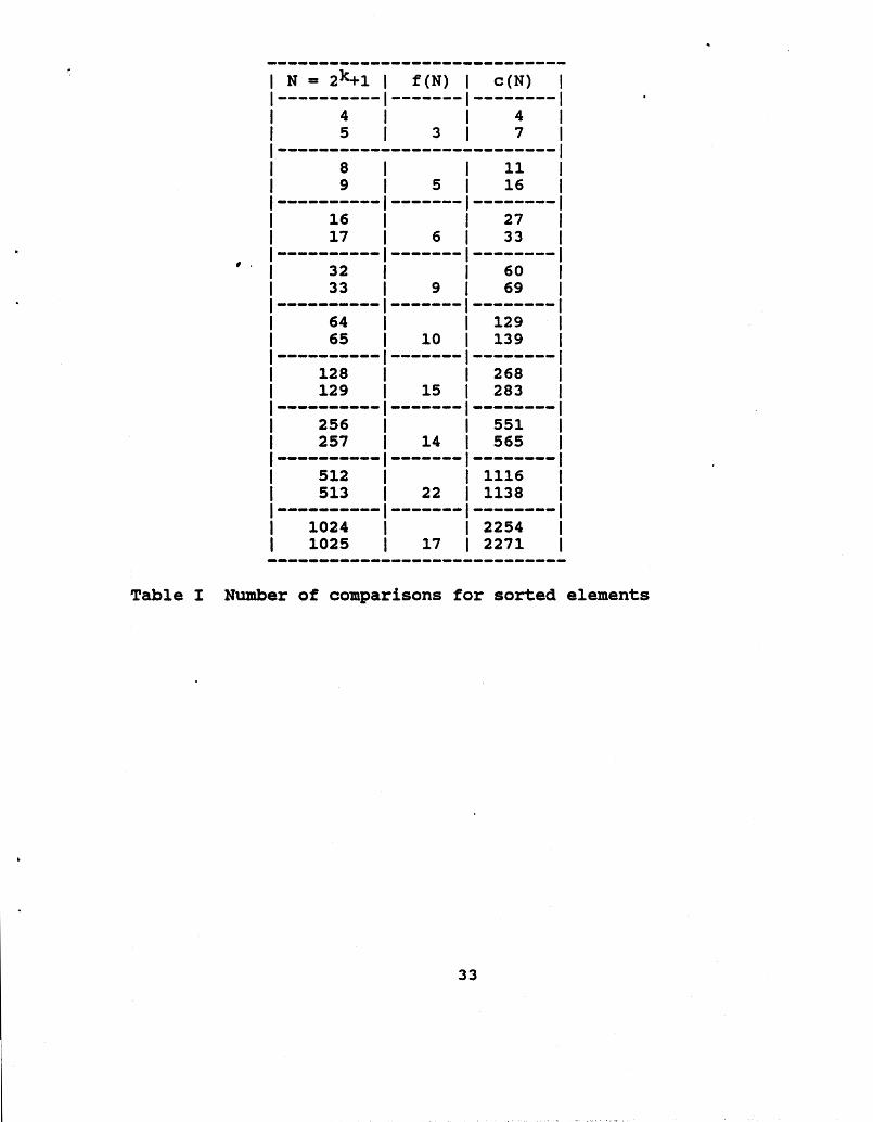
Table I Number of comparisons for sorted elements

As can be seen, f ( N ) does not grow quickly and in general seems to grow as 2*log(N). In the next section, where we report computational experience with TOURNAMENT-SORT!, it will be seen that the number of comparisons remains small even when a certain amount of randomness is reintroduced into the ordering of the elements.

It is considerably more difficult to bound the worst case performance of the algorithm or to determine an exact worst case in practice. From the above analysis, it can be seen that the performance of the algorithm suffers when an element loses a contest to another element which wins a tournament soon afterwards. This puts the former element back into competition quickly and results in more comparisons. Another way of looking at this is that performance is hurt if the node with the larger number of successors wins a contest. This creates nodes with a large number of successors. It also keeps these nodes close to the top of the tree where they are eligible to win a tournament. When such a node wins a tournament, its immediate successors compete in the next tournament.

Unfortunately, this is not provably the worst case. The performance of the algorithm is also affected by which nodes compete with each other in the tournaments. This does not affect the number of comparisons radically: typically it alters the number of comparisons by less than 10%. Nevertheless, this is sufficient to prevent us from obtaining a provable bound.

We believe, however, that the case where the node with the larger number of immediate successors wins each contest is a pathologically bad case. Likewise, the similar case where the node with the largest total number of successors (in the entire subtree rooted at that node) wins each contest is a pathologically bad case. By altering the comparison function passed to the sort to declare the node with the larger number of successors the winner, we were able to test the performance of this sort in these pathological cases. We found the number of comparisons in these cases to be within 5% of the case where the elements were randomly ordered, and as w e shall see, in this case the number of comparisons was of order N*log(N)*(log(log(N)). While this is not a proof that the worst case performance of the algorithm is N*log (N) *log (log (N) ) , we feel that this is strong empirical evidence supporting this hypothesis.

We ran the algorithm on many random data sets of a wide variety of sizes, ranging from 100 elements to 250,000 elements. The table below summarizes the results of these runs, giving the total number of comparisons as a function of the number of elements. The table also gives the ratio of the number of comparisons to N*log (N) and to N*log (N) *log (log (N) ) . As can be seen, the n w e r of comparisons grows slightly more quickly than

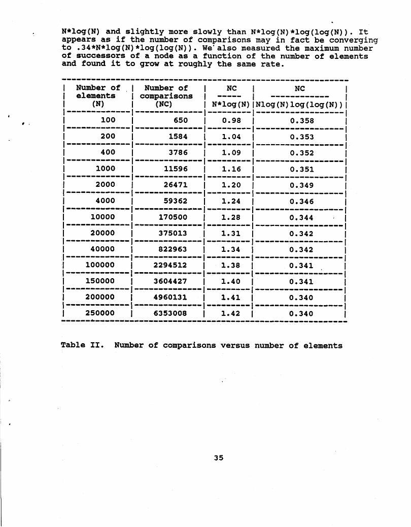
N*log (N) and slightly more slowly than N*log (N) *log (log (N) ) . It appears as if the number of comparisons may in fact be converging to .34*N*log(N)*log(log(N)). We'also measured the maximum number of successors of a node as a function of the number of elements and found it to grow at roughly the same rate.

Fable 11. Number of comparisons versus number of eleaents

As we noted above, TOURNAMENT-SORT! performs much better on already sorted lists. For example, in sorting an already sorted list with 2000 elements it makes 4548 comparisons if the list is sorted in the right direction and 4547 comparisons if the list is sorted in the opposite direction. Actually, it seems that any kind of regularity reduces the number of comparisons, and the worst case is the random list. For example, if we append an already sorted list with 1000 elements to itself (or its reverse) - which is a notoriously bad case for many implementations of quicksort which use llmedian-of-threell partitioning - reduction sort uses just 7631 comparisons when a list is appended to itself and 7581 comparisons when a list is appended to its reverse. Even if we alternate elements from the list with elements from its reverse with the help of something like:

(DEFINE (MIX X Y) (IF (NULL? X)

Y (CONS (CAR X) (MIX Y (CDR X) ) ) ) ) ,

we still make just 10678 comparisons against about 26500 in the random case.

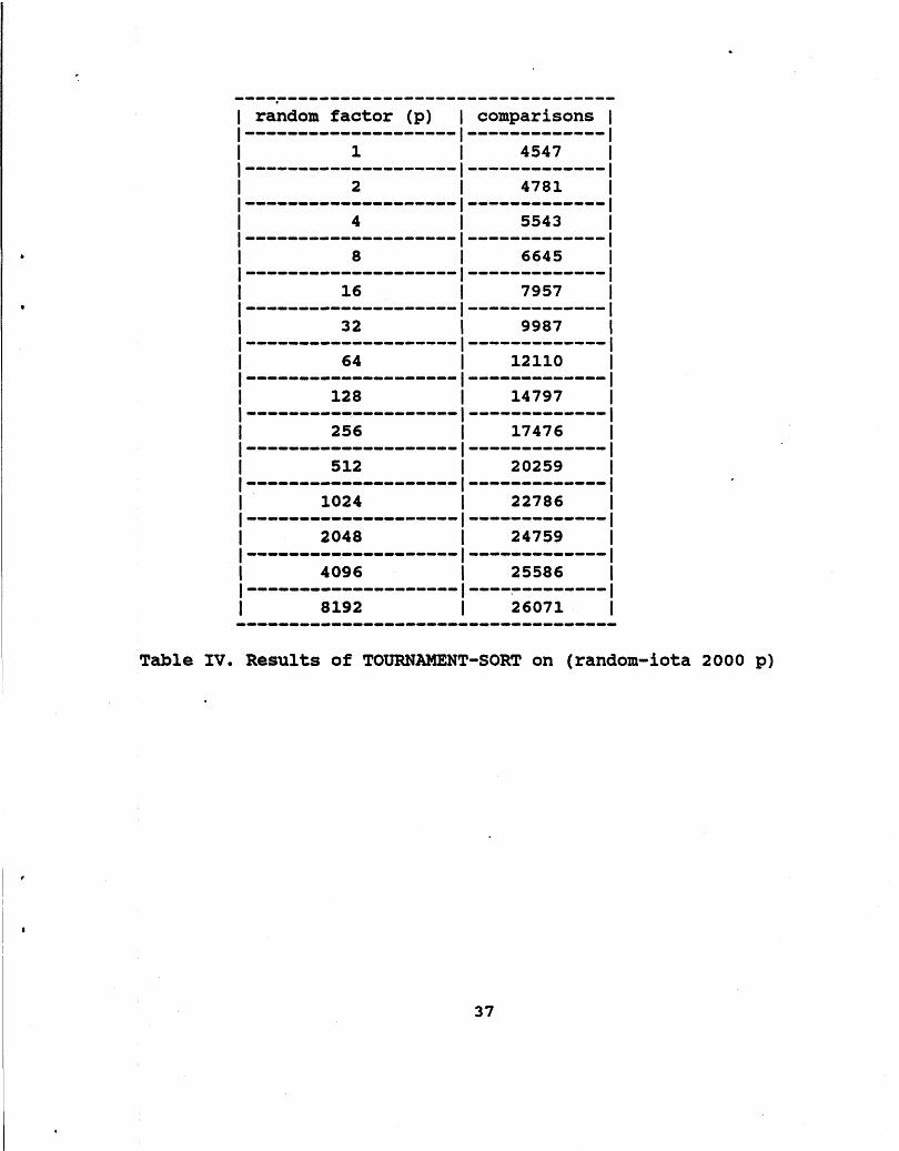
We can measure the effects of the presence of order in data by sorting lists generated by a function:

(DEFINE (RAEJDOH-IOTA N P) (IF (I N 0)

' 0 (CONS (+ N (RANDOM P)) (RANDOM-IOTA (- N

The following tabla includes and numbers of comparisons for lists generated by random-iota with n=2000.

I random factor (p) I comparisons I l-----w~l------l.--.I-I-----.I-.I.II---~

1 4547 I

I I )-------o----------.II-Io--..I)--I.)--I--- I

2 4781 1

I I l-------.-.---.------l------------- I

4 5543 I

I I 1-----.--------------I------------- I

8 6645 I

I I ~---w-~~oo---~~~o.-.-~-------~-----

I

16 7957 I

I I l------~.-o-w---.----l---.--------- I

32 9987 I

I I l---~---.------o-----l----------*-- I

64 12110 I

I I I---o---v--o-o-----.I)-~----C.I).I)------ I

128 14797 I

I I l------..----------.-l---..I)--------- I

256 17476 I

I I ~ ~ ~ ~ ~ ~ ~ ~ ~ ~ ~ o ~ ~ ~ ~ o ~ ~ ~ . I ) ~ o ~ ~ ~ ~ o o ~ ~ ~ ~ ~ l L

I

512 20259 1

I I l----------~---------l------------- I

1024 22786 1

I I ~C-o---~vo------.----~-----------~-

I 1

Table N. Results of TOURNAMENT-SORT on (random-iota 2000 p)

We have presented new sorting algorithms based on the tournament queue data structure and have shown this data structure gives rise to a unified representation of a variety of sorting algorithms, including several of the best known ones and an entirely new algorithm, TOURNAMENT-SORT!. We have also found that the implementations of the algorithms which do the same comparisons as Mergesort, Floyd's Algorithm, and Insertion Sort are more efficient than implementations of these algorithms using more traditional data structures. We have shown the performance of the TOURNAMENT-SORT! to be no worse than order N*log (N) *log (log (N) ) in practice for most cases of interest and to be of order N in the case where the input elements are nearly ordered on input to the algorithm. We have done preliminary computational experiments and shown that the performance of the new algorithm compares very favorably with that of the best known sorting algorithms currently available. We are continuing to do computational experiments to more fully test the algorithm's performance on a wider variety of inputs. We are also continuing to investigate its worst case performance. Finally, we are beginning to experiment with the tournament queue structure as a priority queue.

XI. Biblioaraphx

1. Knuth, Donald E., '#The Art of Computer Programming," vole 3, Addison- Wesley, 1973

2. Sedgewick, Robert, "Algorithms, Addison-Wesley , 1983 3. Gonnet, Gaston H., "Handbook of Algorithms and Data structure^,^ Addison-Wesley, 1984

4. Abelson, Harold, and Gerald Jay Sussman, %tructure and Inter- pretation of Computer program^,^ MIT Press, 1985

5. Clinger, W e (ed.), "The Revised Revised Report on Scheme," MIT A1 Memo No. 848, 1985

6. Brown, Mark R., HImplementation and Analysis of Binomial Queue Algorithms," SIAM Journal of Computing, Vol. 7, No. 3, August 1978

7. Vuillemin, Jean, "A Data Structure for Manipulating Priority Queues," Communications of ACM, Volume 21, No. 4, April 1978

8. Floyd, Robert W., "Algorithm 113. Treesort," Communications of ACM, Volume 5, No. 8, August 1962

9. Williams, J.W.J., nAlgorithm 232. Heapsort," Communications of ACM, Volume 7, NO. 6, June 1964