UVA CS 6316: Machine Learning Lecture 11b: Support Vector ... · Machine Learning Lecture 11b: Support Vector Machine (nonlinear) Kernel Trick and in Practice Dr. YanjunQi University

UVA CS 6316:Machine Learning

Lecture 11b: Support Vector Machine (nonlinear) Kernel Trick and in Practice

Dr. Yanjun Qi

University of VirginiaDepartment of Computer Science

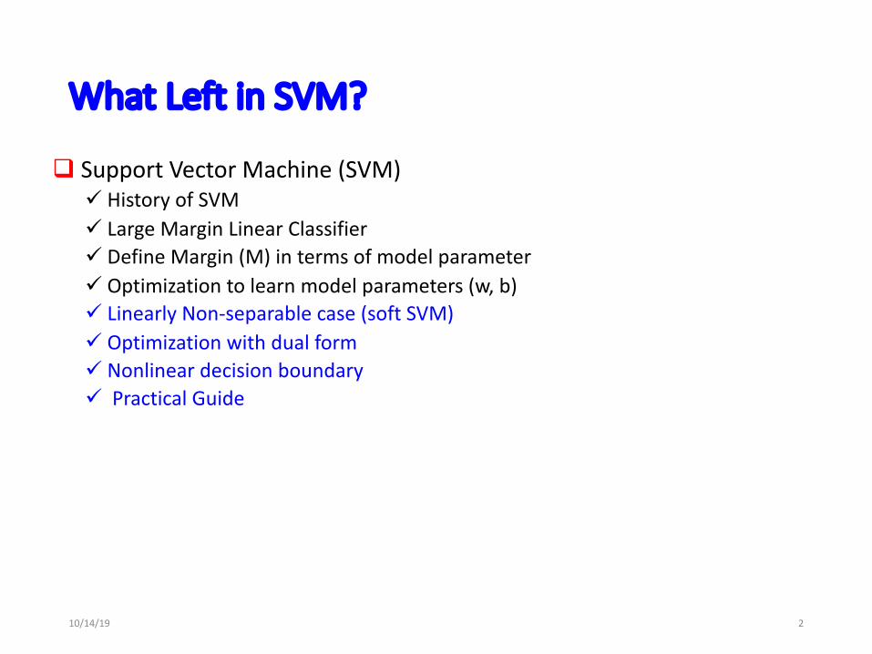
What Left in SVM?

q Support Vector Machine (SVM)ü History of SVM ü Large Margin Linear Classifier ü Define Margin (M) in terms of model parameterü Optimization to learn model parameters (w, b) ü Linearly Non-separable case (soft SVM)ü Optimization with dual form ü Nonlinear decision boundary ü Practical Guide

10/14/19 2

Today

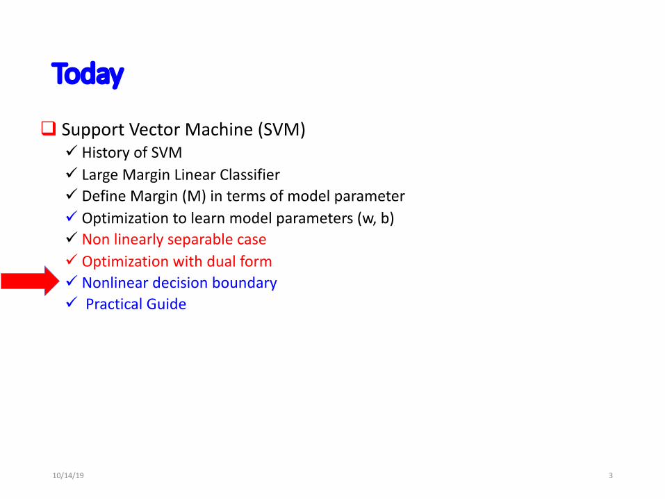
q Support Vector Machine (SVM)ü History of SVM ü Large Margin Linear Classifier ü Define Margin (M) in terms of model parameterü Optimization to learn model parameters (w, b) ü Non linearly separable caseü Optimization with dual form ü Nonlinear decision boundary ü Practical Guide

10/14/19 3

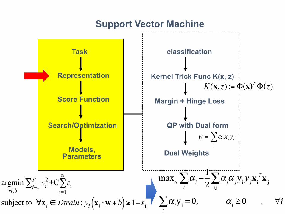
Support Vector Machine

classification

Kernel Trick Func K(x, z)

Margin + Hinge Loss

QP with Dual form

Dual Weights

Task

Representation

Score Function

Search/Optimization

Models, Parameters

€

w = α ixiyii∑

argminw,b

wi2

i=1p∑ +C εi

i=1

n

∑

subject to ∀xi ∈ Dtrain : yi xi ⋅w+b( ) ≥1−εi

K(x, z) :=Φ(x)TΦ(z)

4

maxα α i −i∑ 1

2 α iα jyi y ji,j∑ xi

Txj

α iyi =0i∑ , α i ≥0 ∀i

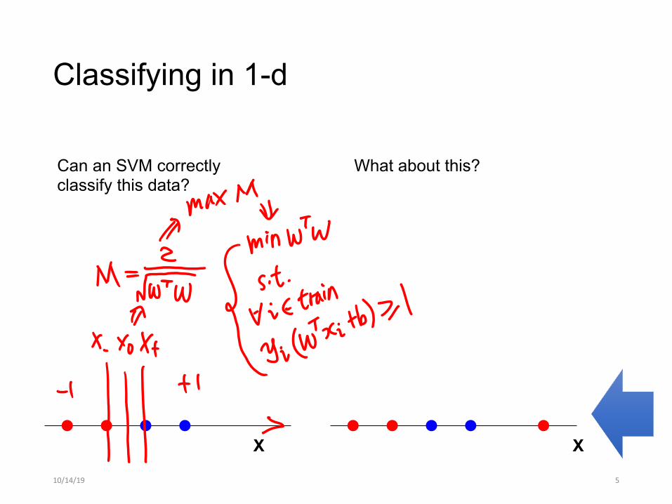
Classifying in 1-d

10/14/19 5

Can an SVM correctly classify this data?

What about this?

X X

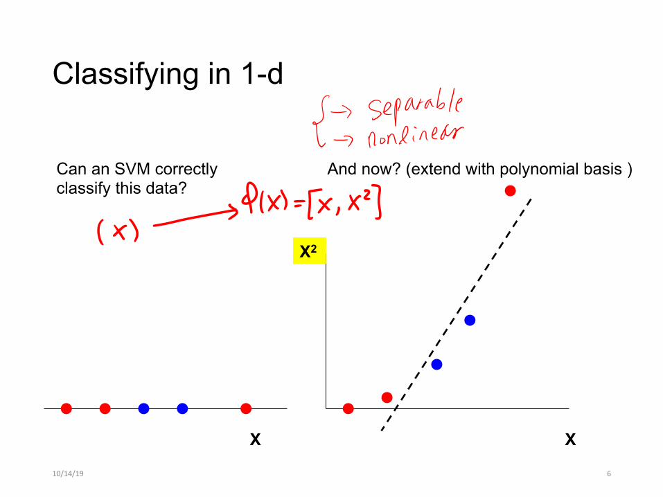
Classifying in 1-d

10/14/19 6

Can an SVM correctly classify this data?

And now? (extend with polynomial basis )

X X

X2

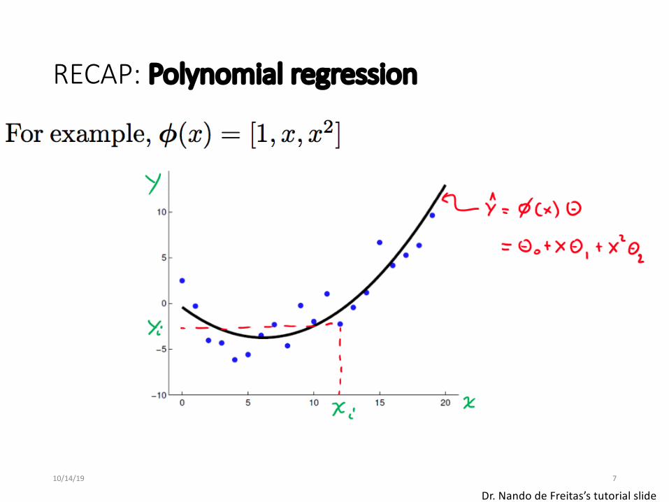
RECAP: Polynomial regression

• Introduce basis functions

10/14/19 7

Dr. Nando de Freitas’s tutorial slide

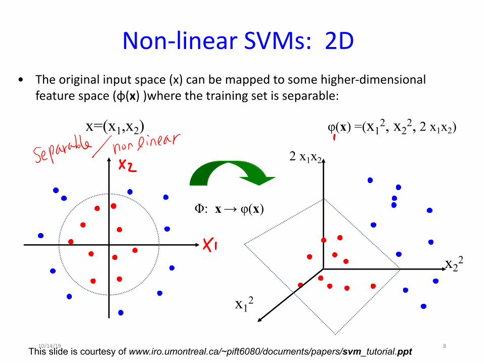
Non-linear SVMs: 2D

This slide is courtesy of www.iro.umontreal.ca/~pift6080/documents/papers/svm_tutorial.ppt

Φ: x→ φ(x)

x12

x22

2 x1x2

x=(x1,x2)

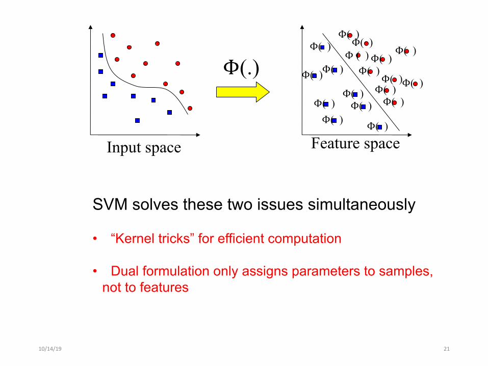
• The original input space (x) can be mapped to some higher-dimensional feature space (φ(x) )where the training set is separable:

φ(x) =(x12, x2

2, 2 x1x2)

810/14/19

10/14/19 9Credit: Stanford ML course

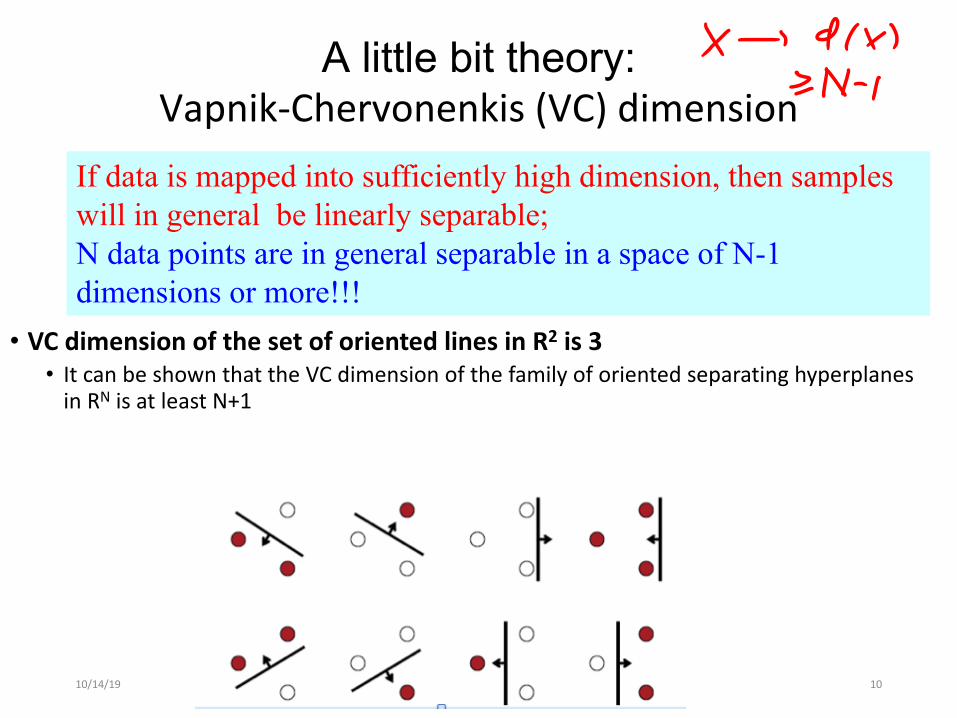
A little bit theory: Vapnik-Chervonenkis (VC) dimension

• VC dimension of the set of oriented lines in R2 is 3• It can be shown that the VC dimension of the family of oriented separating hyperplanes

in RN is at least N+1

10/14/19 10

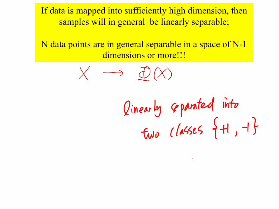
If data is mapped into sufficiently high dimension, then samples will in general be linearly separable; N data points are in general separable in a space of N-1 dimensions or more!!!

Φ( )

Φ( )

Φ( )Φ( )Φ( )

Φ( )

Φ( )Φ( )

Φ(.) Φ( )

Φ( )

Φ( )Φ ( )Φ( )

Φ( )

Φ( )

Φ( )Φ( ) Φ( )

Feature spaceInput space

• Possible problems- High computation burden due to high-dimensionality - Many more parameters to estimate

10/14/19 11

Is this too much computational work?

If data is mapped into sufficiently high dimension, then samples will in general be linearly separable;

N data points are in general separable in a space of N-1 dimensions or more!!!

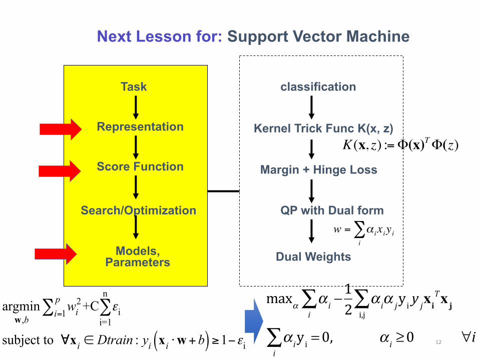
Next Lesson for: Support Vector Machine

classification

Kernel Trick Func K(x, z)

Margin + Hinge Loss

QP with Dual form

Dual Weights

Task

Representation

Score Function

Search/Optimization

Models, Parameters

€

w = α ixiyii∑

argminw,b

wi2

i=1p∑ +C εi

i=1

n

∑



12



Txj

α iyi =0i∑ , α i ≥0 ∀i

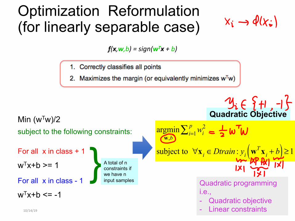
Optimization Reformulation (for linearly separable case)

10/14/19 13

Min (wTw)/2 subject to the following constraints:

For all x in class + 1

wTx+b >= 1

For all x in class - 1

wTx+b <= -1

}A total of n constraints if we have n input samples

argminw,b

wi2

i=1p∑

subject to ∀x i ∈Dtrain : yi wT x i + b( ) ≥1

Quadratic Objective

Quadratic programming i.e., - Quadratic objective - Linear constraints

f(x,w,b) = sign(wTx + b)

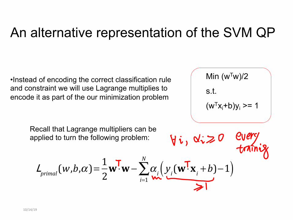
An alternative representation of the SVM QP

10/14/19 14

•Instead of encoding the correct classification rule and constraint we will use Lagrange multiplies to encode it as part of the our minimization problem

Min (wTw)/2

s.t.

(wTxi+b)yi >= 1

Recall that Lagrange multipliers can be applied to turn the following problem:

Lprimal(w ,b,α )=

12w ⋅w− α i yi(w ⋅x i +b)−1( )

i=1

N

∑

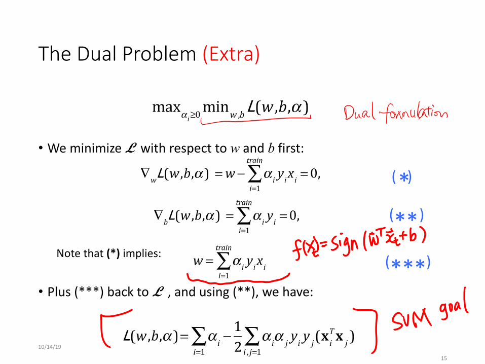
The Dual Problem (Extra)

• We minimize L with respect to w and b first:

Note that (*) implies:

• Plus (***) back to L , and using (**), we have:

10/14/19

15

***( )

maxα i≥0minw ,bL(w ,b,α )

!! ∇wL(w ,b,α )! =w− α i yixi =0

i=1

train

∑ ,

!! ∇bL(w ,b,α )! = α i yi =0

i=1

train

∑ ,

!!w = α i yixi

i=1

train

∑

*( )

!!! L(w ,b,α )= α i

i=1∑ − 12 α iα j yi y j(x iTx j )

i , j=1∑

**( )

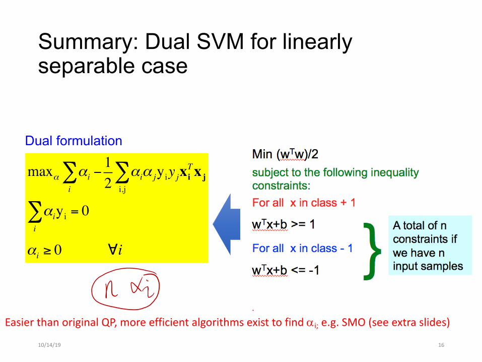
Summary: Dual SVM for linearly separable case

10/14/19 16

Dual formulation

maxα αi −i∑ 1

2αiα jyiyj

i,j∑ xi

Txj

αiyi = 0i∑

αi ≥ 0 ∀i

Easier than original QP, more efficient algorithms exist to find ai; e.g. SMO (see extra slides)

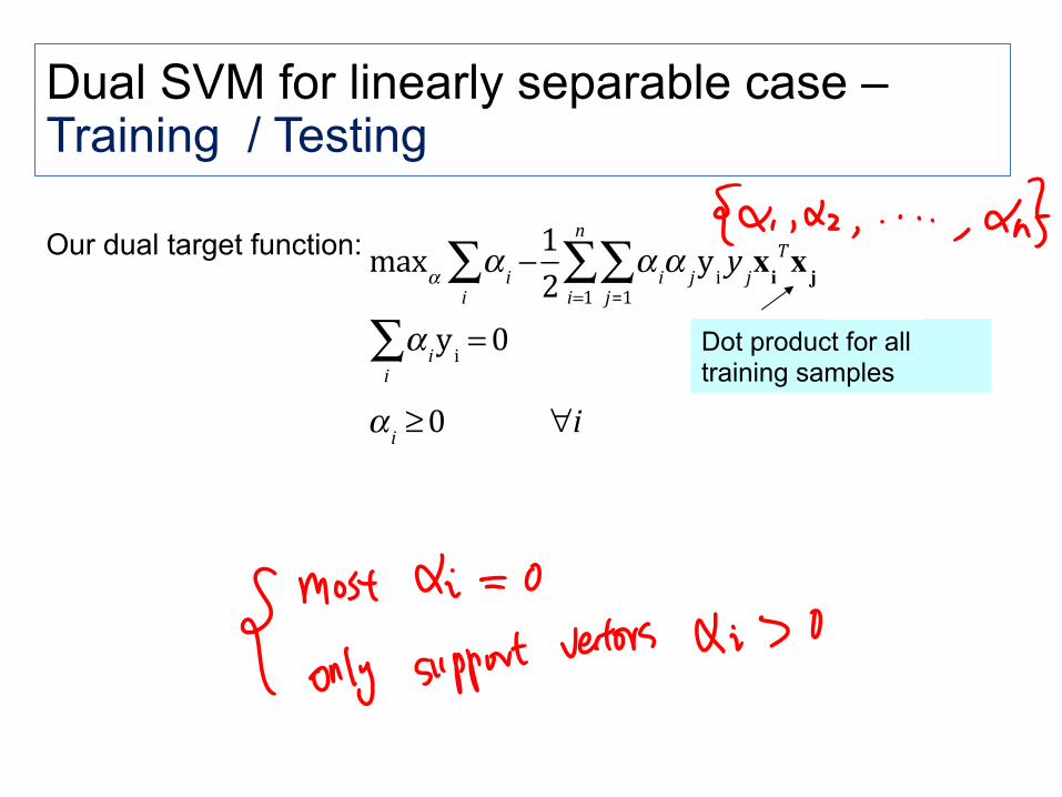
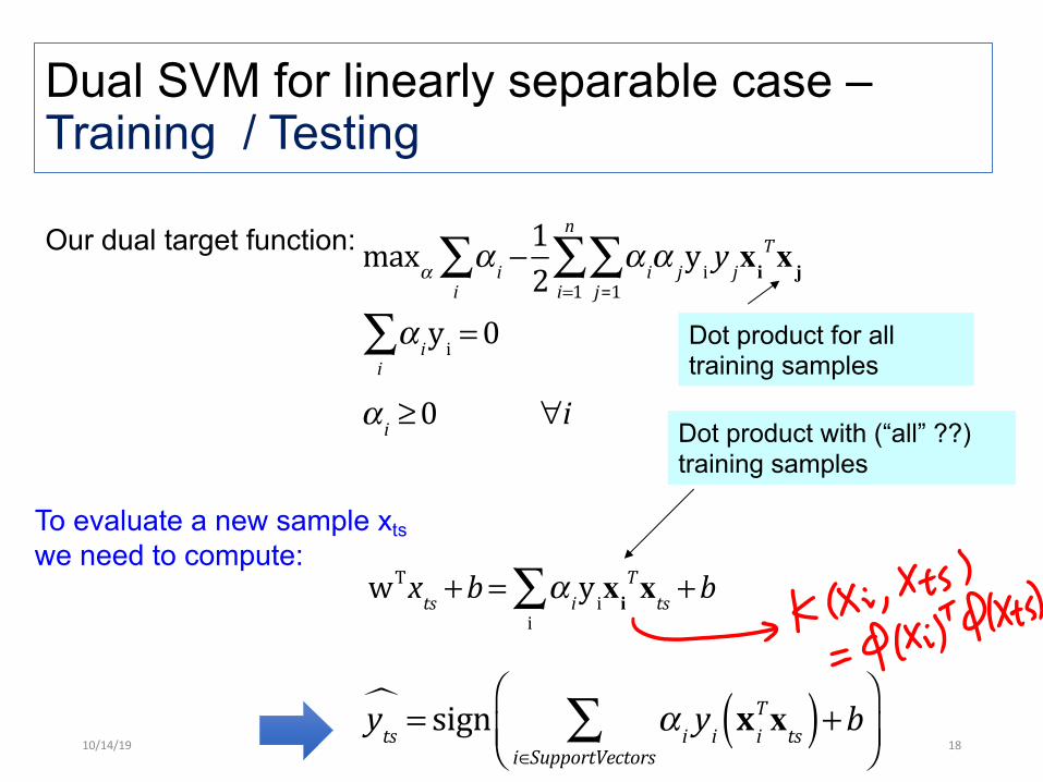
Dual SVM for linearly separable case –Training / Testing

10/14/19 17

Our dual target function:


2 α iα jyi y jxiTxjj=1∑

i=1

n

∑α iyi =0

i∑α i ≥0 ∀i

Dot product for all training samples

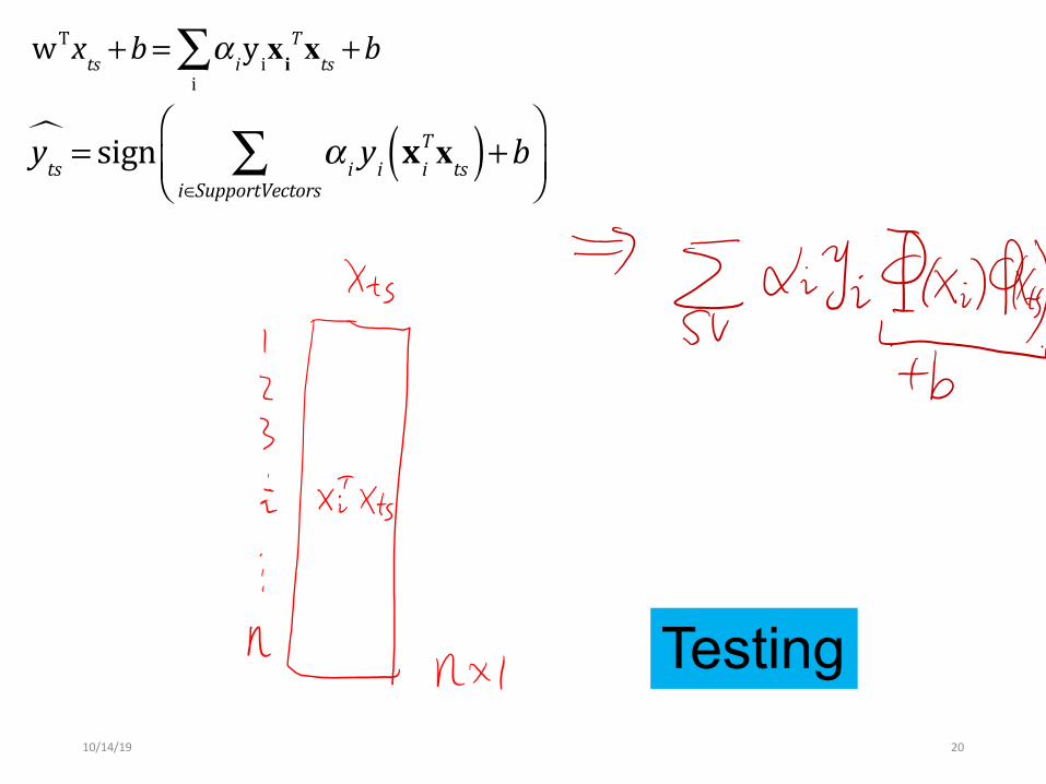
To evaluate a new sample xtswe need to compute:

!!wTxts +b= α iyi

i∑ xi

Txts +b

yts! = sign α i yi x i

Txts( )i∈SupportVectors

∑ +b⎛

⎝⎜⎞

⎠⎟

Dual SVM for linearly separable case –Training / Testing

10/14/19 18

Our dual target function:


2 α iα jyi y jxiTxjj=1∑

i=1

n

∑α iyi =0

i∑α i ≥0 ∀i

Dot product for all training samples

To evaluate a new sample xtswe need to compute:

!!wTxts +b= α iyi

i∑ xi

Txts +b

Dot product with (“all” ??) training samples



∑ +b⎛

⎝⎜⎞

⎠⎟

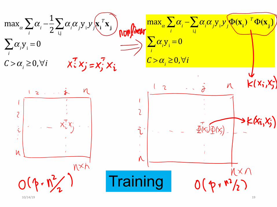
10/14/19 19

maxα α i −i∑ α iα jyi y j

i,j∑ Φ(xi )

TΦ(xj)

α iyi =0i∑C >α i ≥0,∀i



Txj

α iyi =0i∑C >α i ≥0,∀i

Training

10/14/19 20

!!wTxts +b= α iyi

i∑ xi

Txts +b



∑ +b⎛

⎝⎜⎞

⎠⎟

Testing

Φ( )

Φ( )

Φ( )Φ( )Φ( )

Φ( )

Φ( )Φ( )

Φ(.) Φ( )

Φ( )

Φ( )Φ ( )Φ( )

Φ( )

Φ( )

Φ( )Φ( ) Φ( )

Feature spaceInput space

10/14/19 21

SVM solves these two issues simultaneously

• “Kernel tricks” for efficient computation

• Dual formulation only assigns parameters to samples, not to features

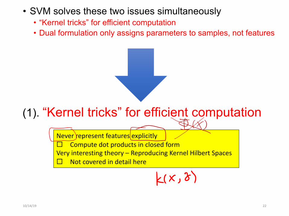
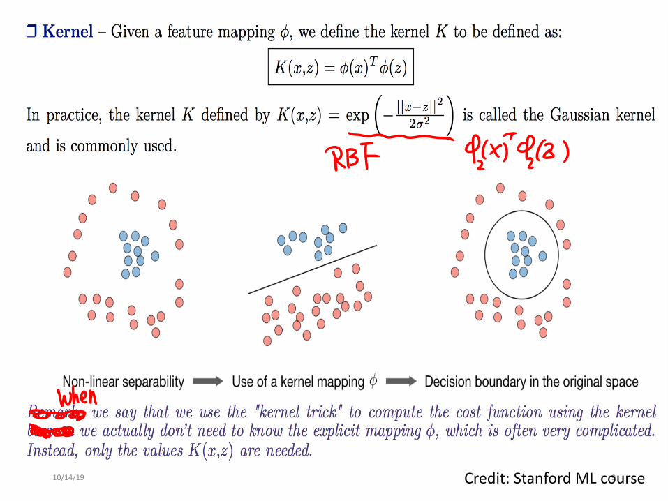
(1). “Kernel tricks” for efficient computation

• SVM solves these two issues simultaneously• “Kernel tricks” for efficient computation • Dual formulation only assigns parameters to samples, not features

10/14/19 22

Never represent features explicitly¨ Compute dot products in closed formVery interesting theory – Reproducing Kernel Hilbert Spaces ¨ Not covered in detail here

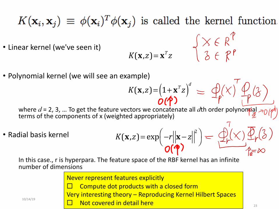
• Linear kernel (we've seen it)

• Polynomial kernel (we will see an example)

where d = 2, 3, … To get the feature vectors we concatenate all dth order polynomial terms of the components of x (weighted appropriately)

• Radial basis kernel

In this case., r is hyperpara. The feature space of the RBF kernel has an infinite number of dimensions

10/14/19

23

K(x ,z)= xTz

K(x ,z)= 1+ xTz( )d

K(x ,z)= exp −r x− z

2⎛⎝

⎞⎠

Never represent features explicitly¨ Compute dot products with a closed formVery interesting theory – Reproducing Kernel Hilbert Spaces ¨ Not covered in detail here

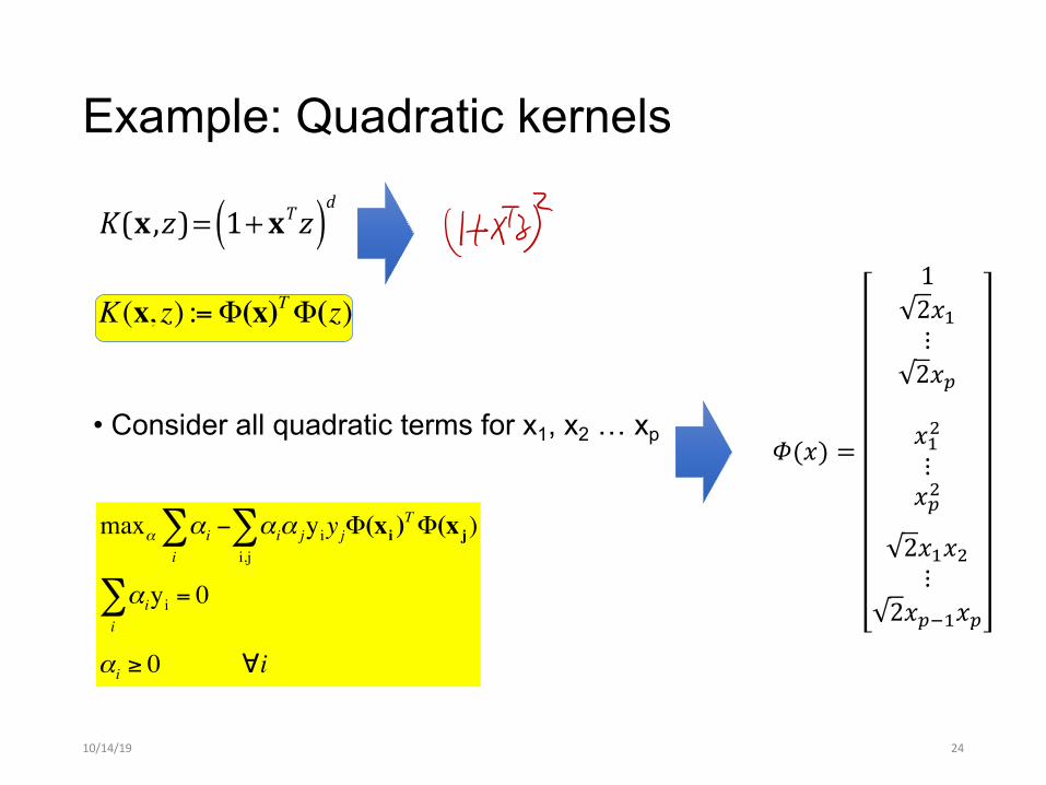
Example: Quadratic kernels

10/14/19 24

maxα αi −i∑ αiα jyiyj

i,j∑ Φ(xi )

TΦ(x j)

αiyi = 0i∑

αi ≥ 0 ∀i

• Consider all quadratic terms for x1, x2 … xp


K(x ,z)= 1+ xTz( )d

𝛷(𝑥) =

12𝑥(⋮2𝑥*

𝑥(+⋮𝑥*+

2𝑥(𝑥+⋮

2𝑥*,(𝑥*

10/14/19 25

K(x ,z)= 1+ xTz( )d

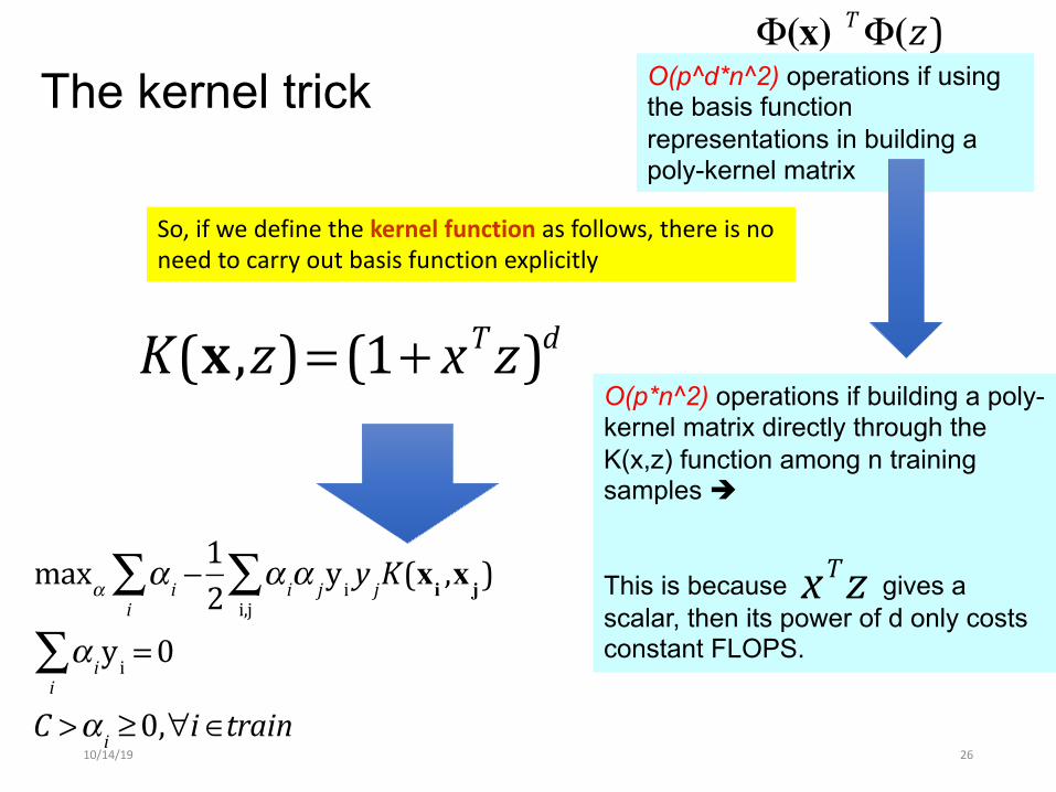
The kernel trick

10/14/19 26

So, if we define the kernel function as follows, there is no need to carry out basis function explicitly

K(x ,z)= (1+ xTz)d

!!


2 α iα jyi y ji,j∑ K(xi ,xj)

α iyi =0i∑C >α i ≥0,∀i∈train

O(p*n^2) operations if building a poly-kernel matrix directly through the K(x,z) function among n training samples è

This is because gives a scalar, then its power of d only costs constant FLOPS.

O(p^d*n^2) operations if using the basis function representations in building a poly-kernel matrix

xTz

Φ(x)TΦ(z)

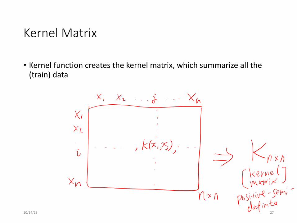
Kernel Matrix

• Kernel function creates the kernel matrix, which summarize all the (train) data

10/14/19 27

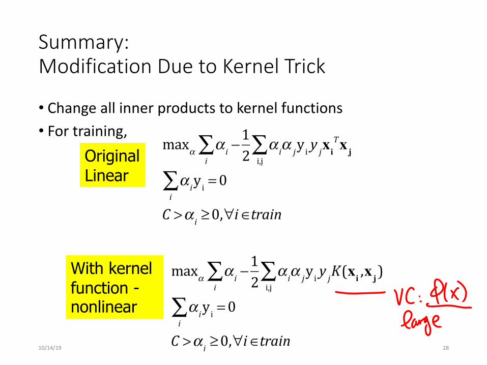
Summary: Modification Due to Kernel Trick

• Change all inner products to kernel functions• For training,

10/14/19 28

Original Linear

With kernel function -nonlinear

!!



Txj


!!


2 α iα jyi y ji,j∑ K(xi ,xj)


Summary: Modification Due to Kernel Trick

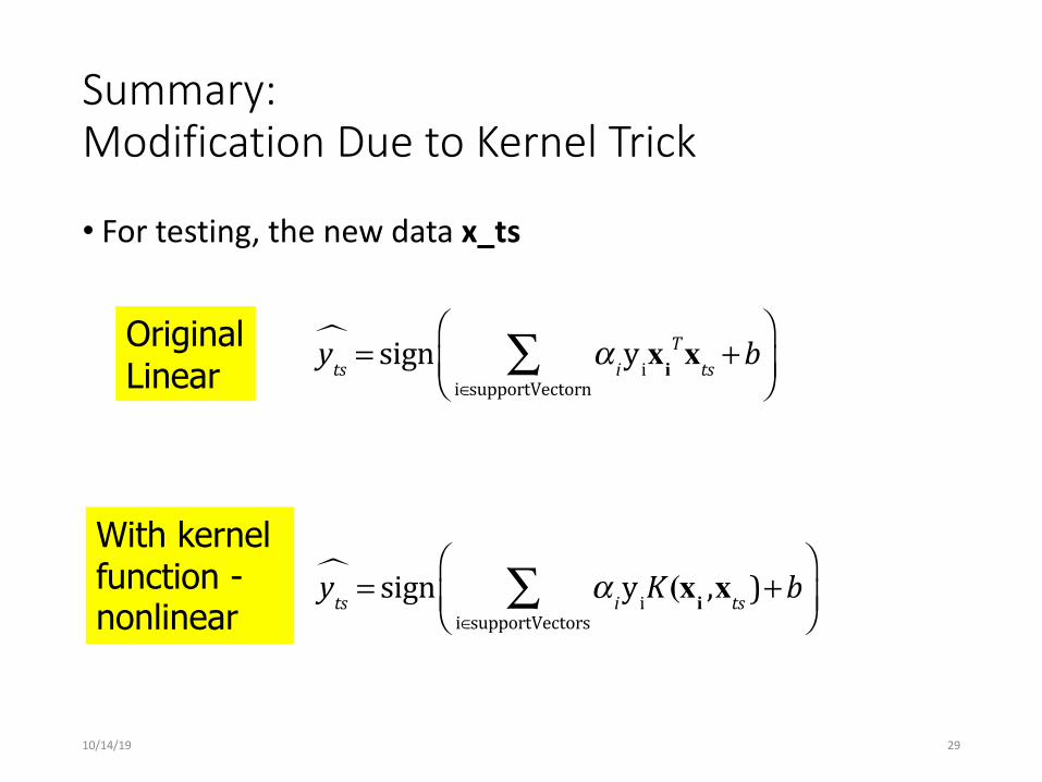
• For testing, the new data x_ts

10/14/19 29

yts! = sign α iyi

i∈supportVectors∑ K (xi ,xts )+b

⎛

⎝⎜⎞

⎠⎟

Original Linear

With kernel function -nonlinear

yts! = sign α iyi

i∈supportVectorn∑ xi

Txts +b⎛

⎝⎜⎞

⎠⎟

Kernel Trick: Implicit Basis Representation

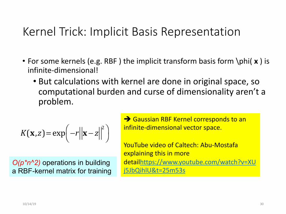
• For some kernels (e.g. RBF ) the implicit transform basis form \phi( x ) is infinite-dimensional!

• But calculations with kernel are done in original space, so computational burden and curse of dimensionality aren’t a problem.

10/14/19 30

K(x ,z)= exp −r x− z

2⎛⎝

⎞⎠

è Gaussian RBF Kernel corresponds to an infinite-dimensional vector space.

YouTube video of Caltech: Abu-Mostafaexplaining this in more detailhttps://www.youtube.com/watch?v=XUj5JbQihlU&t=25m53s

O(p*n^2) operations in building a RBF-kernel matrix for training

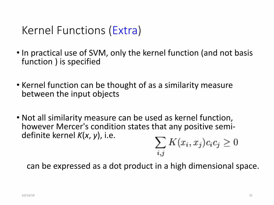
https://www.youtube.com/watch?v=XUj5JbQihlU&t=25m53s

Kernel Functions (Extra)

• In practical use of SVM, only the kernel function (and not basis function ) is specified

• Kernel function can be thought of as a similarity measure between the input objects

• Not all similarity measure can be used as kernel function, however Mercer's condition states that any positive semi-definite kernel K(x, y), i.e.

can be expressed as a dot product in a high dimensional space.

10/14/19 31

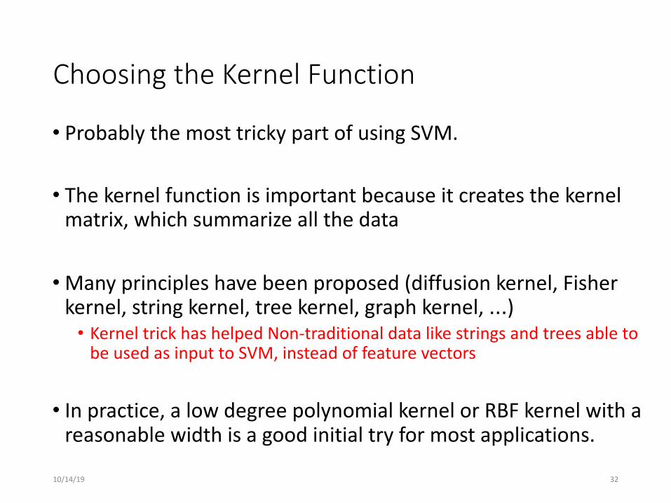
Choosing the Kernel Function

• Probably the most tricky part of using SVM.

• The kernel function is important because it creates the kernel matrix, which summarize all the data

• Many principles have been proposed (diffusion kernel, Fisher kernel, string kernel, tree kernel, graph kernel, …)

• Kernel trick has helped Non-traditional data like strings and trees able to be used as input to SVM, instead of feature vectors

• In practice, a low degree polynomial kernel or RBF kernel with a reasonable width is a good initial try for most applications.

10/14/19 32

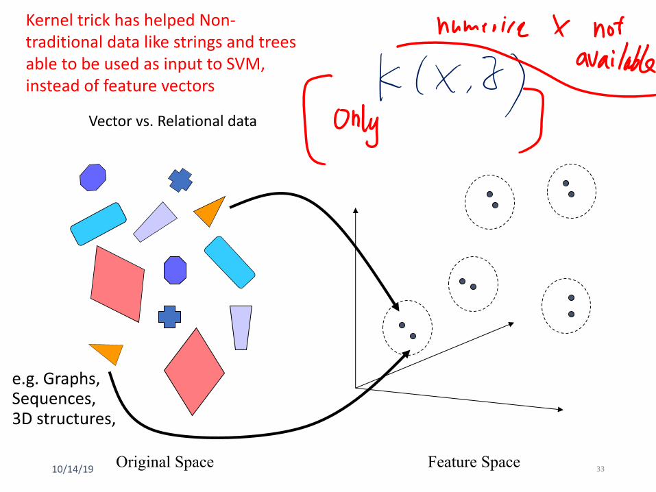
Original Space Feature Space

Vector vs. Relational data

e.g. Graphs,Sequences,3D structures,

10/14/19 33

Kernel trick has helped Non-traditional data like strings and trees able to be used as input to SVM, instead of feature vectors

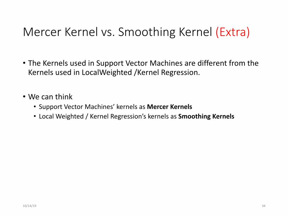
Mercer Kernel vs. Smoothing Kernel (Extra)

• The Kernels used in Support Vector Machines are different from the Kernels used in LocalWeighted /Kernel Regression.

• We can think • Support Vector Machines’ kernels as Mercer Kernels • Local Weighted / Kernel Regression’s kernels as Smoothing Kernels

10/14/19 34

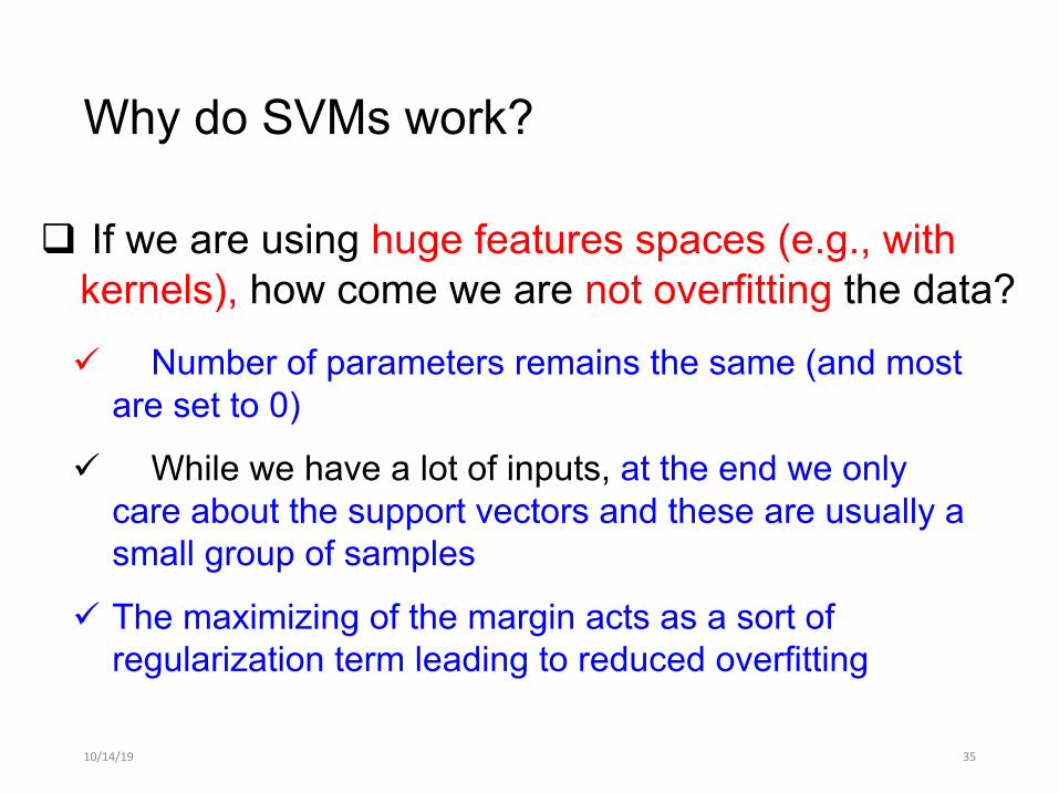
Why do SVMs work?

10/14/19 35

q If we are using huge features spaces (e.g., with kernels), how come we are not overfitting the data?

ü Number of parameters remains the same (and most are set to 0)

ü While we have a lot of inputs, at the end we only care about the support vectors and these are usually a small group of samples

ü The maximizing of the margin acts as a sort of regularization term leading to reduced overfitting

10/14/19 36

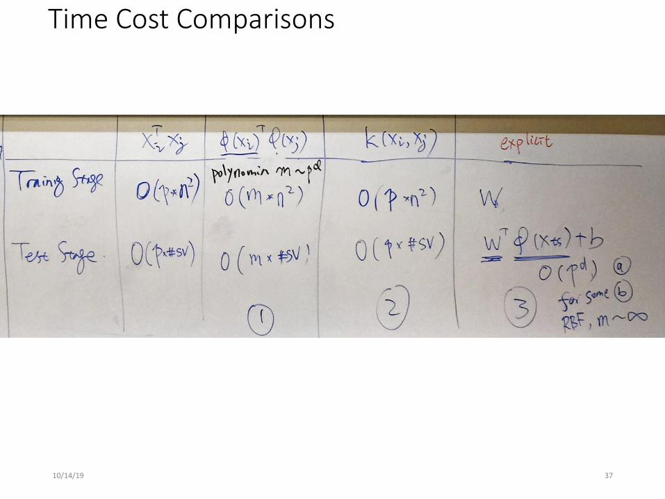
Time Cost Comparisons

10/14/19 37

Today


10/14/19 38

Software

• A list of SVM implementation can be found at • http://www.kernel-machines.org/software.html

• Some implementation (such as LIBSVM) can handle multi-class classification

• SVMLight is among one of the earliest implementation of SVM

• Several Matlab toolboxes for SVM are also available

10/14/19 39

Summary: Steps for Using SVM in HW

• Prepare the feature-data matrix • Select the kernel function to use• Select the parameter of the kernel function and the value

of C (see next 11c slides for details)• Execute the training algorithm and obtain the \ai

• Unseen data can be classified using the ai and the support vectors

10/14/19 40

Practical Guide to SVM

• From authors of as LIBSVM: • A Practical Guide to Support Vector Classification Chih-Wei Hsu, Chih-Chung

Chang, and Chih-Jen Lin, 2003-2010 • http://www.csie.ntu.edu.tw/~cjlin/papers/guide/guide.pdf

10/14/19 41

http://www.csie.ntu.edu.tw/~cjlin/papers/guide/guide.pdf

LIBSVM

• http://www.csie.ntu.edu.tw/~cjlin/libsvm/üDeveloped by Chih-Jen Lin etc.üTools for Support Vector classification üAlso support multi-class classification üC++/Java/Python/Matlab/Perl wrappersüLinux/UNIX/WindowsüSMO implementation, fast!!!

10/14/19 42

A Practical Guide to Support Vector Classification

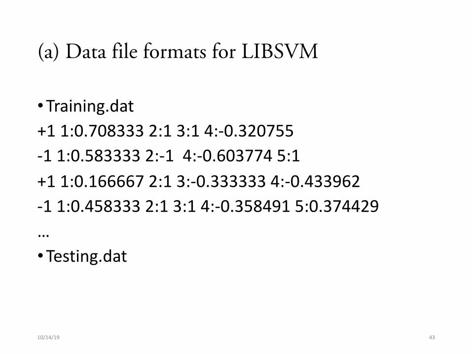
http://www.csie.ntu.edu.tw/~cjlin/libsvm/

(a) Data file formats for LIBSVM

• Training.dat+1 1:0.708333 2:1 3:1 4:-0.320755-1 1:0.583333 2:-1 4:-0.603774 5:1+1 1:0.166667 2:1 3:-0.333333 4:-0.433962-1 1:0.458333 2:1 3:1 4:-0.358491 5:0.374429…• Testing.dat

10/14/19 43

(b) Feature Preprocessing

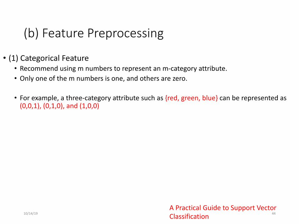
• (1) Categorical Feature • Recommend using m numbers to represent an m-category attribute. • Only one of the m numbers is one, and others are zero.

• For example, a three-category attribute such as {red, green, blue} can be represented as (0,0,1), (0,1,0), and (1,0,0)

10/14/19 44A Practical Guide to Support Vector Classification

Feature Preprocessing

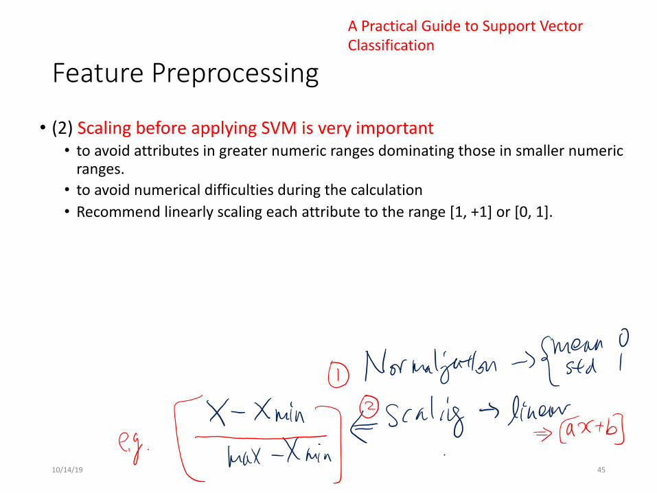
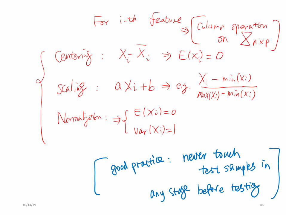
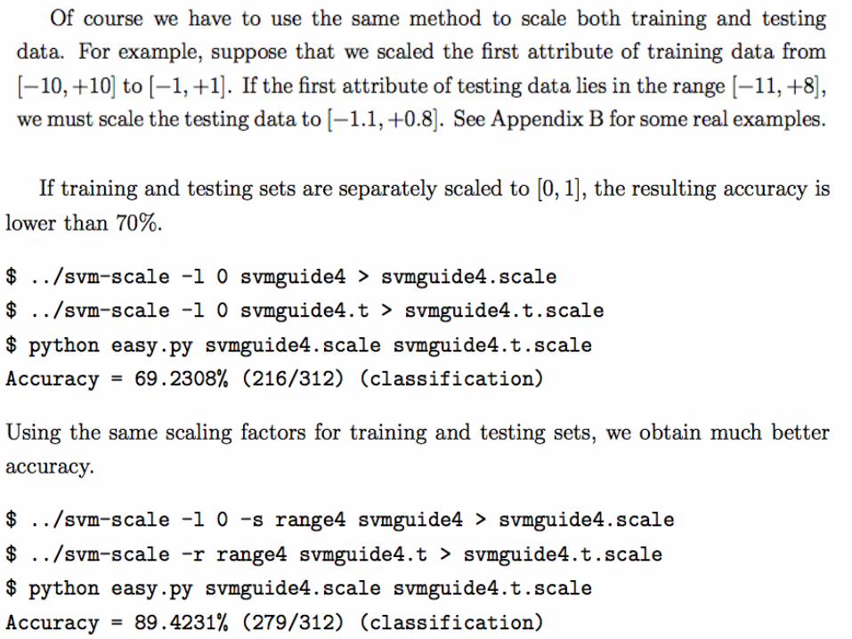
• (2) Scaling before applying SVM is very important • to avoid attributes in greater numeric ranges dominating those in smaller numeric

ranges. • to avoid numerical difficulties during the calculation • Recommend linearly scaling each attribute to the range [1, +1] or [0, 1].

10/14/19 45

A Practical Guide to Support Vector Classification

10/14/19 46




• (3) missing value• Very very tricky ! • Easy way: to substitute the missing values by the mean value of the variable• A little bit harder way: imputation using nearest neighbors• Even more complex: e.g. EM based (beyond the scope)



• (4) out of dictionary token issue • For discrete feature variable, very trick to handle • Easy way: to substitute the values by the most likely value (in train) of the

variable• Easy way: to substitute the values by a random value (in train) of the variable• More solutions later in the NaiveBayes slides!

10/14/19 49

Today: Nonlinear SVM & Practical Guide


ü File format / LIBSVMü Feature preprocsssingü Model selection ü Pipeline procedure

10/14/19 50

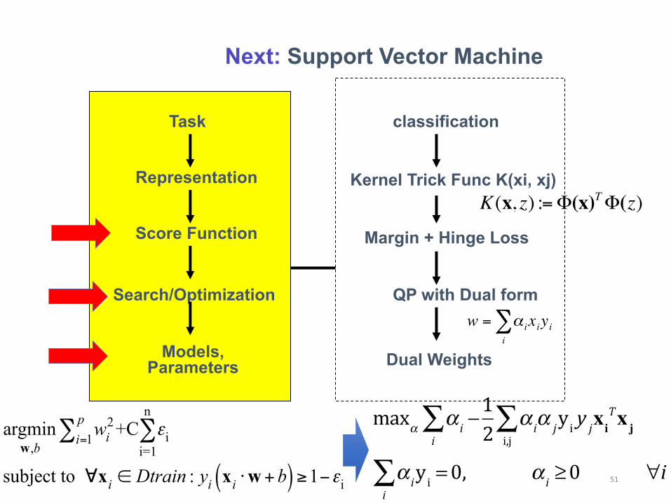
Next: Support Vector Machine

classification

Kernel Trick Func K(xi, xj)

Margin + Hinge Loss

QP with Dual form

Dual Weights

Task

Representation

Score Function

Search/Optimization

Models, Parameters

€

w = α ixiyii∑

argminw,b

wi2

i=1p∑ +C εi

i=1

n

∑



51



Txj

α iyi =0i∑ , α i ≥0 ∀i

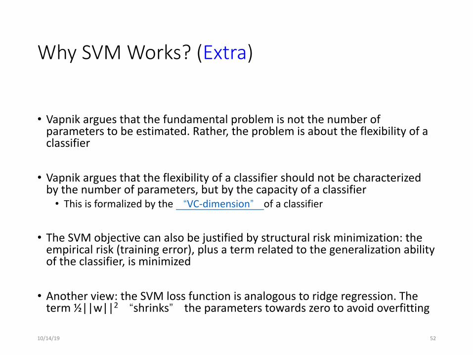
Why SVM Works? (Extra)

• Vapnik argues that the fundamental problem is not the number of parameters to be estimated. Rather, the problem is about the flexibility of a classifier

• Vapnik argues that the flexibility of a classifier should not be characterized by the number of parameters, but by the capacity of a classifier

• This is formalized by the “VC-dimension” of a classifier

• The SVM objective can also be justified by structural risk minimization: the empirical risk (training error), plus a term related to the generalization ability of the classifier, is minimized

• Another view: the SVM loss function is analogous to ridge regression. The term ½||w||2“shrinks” the parameters towards zero to avoid overfitting

10/14/19 52

References

• Big thanks to Prof. Ziv Bar-Joseph and Prof. Eric Xing @ CMU for allowing me to reuse some of his slides

• Elements of Statistical Learning, by Hastie, Tibshirani and Friedman• Prof. Andrew Moore @ CMU’s slides• Tutorial slides from Dr. Tie-Yan Liu, MSR Asi• A Practical Guide to Support Vector Classification Chih-Wei Hsu,

Chih-Chung Chang, and Chih-Jen Lin, 2003-2010• Tutorial slides from Stanford “Convex Optimization I — Boyd &

Vandenberghe

10/14/19 53

Documents

UVA CS 6316: Machine Learning Lecture 11b: Support Vector ... · Machine Learning Lecture 11b: Support Vector Machine (nonlinear) Kernel Trick and in Practice Dr. YanjunQi University