Embed Size (px)
Citation preview
UvA-DARE is a service provided by the library of the University of Amsterdam (http://dare.uva.nl)
UvA-DARE (Digital Academic Repository)
Correlation functions of in- and out-of-equilibrium integrable models
De Nardis, J.
Link to publication
Citation for published version (APA):De Nardis, J. (2015). Correlation functions of in- and out-of-equilibrium integrable models
General rightsIt is not permitted to download or to forward/distribute the text or part of it without the consent of the author(s) and/or copyright holder(s),other than for strictly personal, individual use, unless the work is under an open content license (like Creative Commons).
Disclaimer/Complaints regulationsIf you believe that digital publication of certain material infringes any of your rights or (privacy) interests, please let the Library know, statingyour reasons. In case of a legitimate complaint, the Library will make the material inaccessible and/or remove it from the website. Please Askthe Library: http://uba.uva.nl/en/contact, or a letter to: Library of the University of Amsterdam, Secretariat, Singel 425, 1012 WP Amsterdam,The Netherlands. You will be contacted as soon as possible.
Download date: 05 Jul 2018

10 mm
Jacopo De N
ardisC
orrelation functions of in- and out - of - equilibrium integrable m
odelsJacopo De Nardis
Correlation functions of in- and out - of - equilibrium
integrable models

Correlation functions of in- andout-of-equilibriumintegrable models
ACADEMISCH PROEFSCHRIFT
ter verkrijging van de graad van doctor
aan de Universiteit van Amsterdam
op gezag van de Rector Magnicus
prof. dr. D.C. van den Boom
ten overstaan van een door het College voor Promoties
ingestelde commissie,
in het openbaar te verdedigen in de Agnietenkapel
op vrijdag 25 september 2015, te 12:00 uur
door
Jacopo De Nardisgeboren te Pisa, Italië
Promotiecommissie
Promotor: Prof. dr. J.-S. CauxCopromotor: Prof. dr. C.J.M. Schoutens
Overige leden: Prof. dr. B. Nienhuisdr. V. Gritsevdr. D. Hofman
Prof. dr. J. EisertProf. dr. F. EsslerProf. dr. T. Prosen
Faculteit der Natuurwetenschappen, Wiskunde en Informatica
The research described in this thesis is part of the research programme of theFoundation for Fundamental Research on Matter (FOM), which is part of theNether-lands Organisation for Scientic Research (NWO) andwas carried out at the Insituteof Physics, University of Amsterdam in The Netherlands.

List of publications
This thesis is based on the following publications:
[1] Solution for an interaction quench in the Lieb-Liniger Bose gasJ De Nardis, B Wouters, M Brockmann, J-S CauxPhys. Rev. A 89 033601 (2014)
[2] A Gaudin-like determinant for overlaps of Neel and XXZ Bethe statesM Brockmann, J De Nardis, B Wouters, J-S CauxJ. Phys. A: Math. Theor. 47 145003 (2014)
[3] Neel-XXZ state overlaps: odd particle numbersand Lieb-Liniger scaling limitM Brockmann, J De Nardis, B Wouters, J-S CauxJ. Phys. A: Math. Theor. 47 345003 (2014)
[4] Quenching the Anisotropic Heisenberg Chain: Exact Solutionand Generalized Gibbs Ensemble PredictionsB Wouters, J De Nardis, M Brockmann, D Fioretto,M Rigol, J-S CauxPhys. Rev. Lett. 113 117202 (2014)
[5] Quench action approach for releasing the Neel stateinto the spin-1/2 XXZ chainM Brockmann, B Wouters, D Fioretto, J De Nardis,R Vlijm, J-S CauxJ. Stat. Mech.: Th. Exp. P12009 (2014)
[6] Analytical expression for a post-quench time evolutionof the one-body density matrix of one-dimensional hard-core bosonsJ De Nardis and J-S CauxJ. Stat. Mech.: Th. Exp. P12012 (2014)
[7] Density form factors of the 1D Bose gas for nite entropy statesJ De Nardis and M PanlJ. Stat. Mech.: Th. Exp. P02019 (2015)

[8] Relaxation dynamics of local observables in integrable systemsJ De Nardis, L Piroli and J-S CauxarXiv:1505.03080 (2015)
Other publications from the same author:
[9] Metastable criticality and the super Tonks-Girardeau gasM Panl, J De Nardis and J-S CauxPhys. Rev. Lett. 110 125302 (2013)
Contents
1 Introduction 11.1 Equilibrium many-body physics in one dimension . . . . . . . . . 31.2 Out-of-equilibrium many-body physics . . . . . . . . . . . . . . . 61.3 Out-of-equilibrium integrable models . . . . . . . . . . . . . . . . 111.4 Outline of the thesis . . . . . . . . . . . . . . . . . . . . . . . . . . . 17
2 Integrability and Bethe Ansatz 192.1 Quantum Integrability and the Bethe wave function . . . . . . . . 202.2 Coordinate Bethe ansatz for the Lieb-Liniger model . . . . . . . . 272.3 Algebraic Bethe Ansatz . . . . . . . . . . . . . . . . . . . . . . . . . 31
2.3.1 Solution of the quantum inverse problem . . . . . . . . . . 362.3.2 Scalar products and norms . . . . . . . . . . . . . . . . . . 37
2.4 A lattice statistical model: the 6-vertex model . . . . . . . . . . . . 392.4.1 Quantum Transfer Matrix approach at nite temperature . 40
3 Overlaps in integrable models 433.1 The BEC to Lieb-Liniger overlap . . . . . . . . . . . . . . . . . . . 44
3.1.1 Derivation of the exact overlap formula for N 2 . . . . . 493.1.2 The exact overlap formula . . . . . . . . . . . . . . . . . . . 503.1.3 Connections with Kardar-Parisi-Zhang equation . . . . . . 51
3.2 The overlap of the Néel state with XXZ Bethe states . . . . . . . . 533.2.1 The XXZ spin-1/2 chain . . . . . . . . . . . . . . . . . . . . 543.2.2 The domain wall and the Néel initial state overlaps . . . . 553.2.3 Overlaps between parity invariant XXZ Bethe states and
the Néel state . . . . . . . . . . . . . . . . . . . . . . . . . . 56
4 Thermodynamic limit of integrable models 634.1 Thermodynamic Bethe states . . . . . . . . . . . . . . . . . . . . . 644.2 Thermodynamic Bethe Ansatz for the Lieb-Liniger model . . . . . 684.3 Thermodynamic limit of correlation functions . . . . . . . . . . . 694.4 Thermodynamic form factors . . . . . . . . . . . . . . . . . . . . . 73
4.4.1 Density form factors for nite entropy states . . . . . . . . 794.5 Thermodynamic limit of overlaps and quench action approach . . 87
4.5.1 Single-particle overlap coecients: a conjecture . . . . . . 92
5 The BEC quench in the Lieb-Liniger model 955.1 The problem with the GGE . . . . . . . . . . . . . . . . . . . . . . 965.2 Thermodynamic limit of the overlaps . . . . . . . . . . . . . . . . . 985.3 Explicit solution of the saddle point equation . . . . . . . . . . . . 1005.4 Physical properties of the steady state . . . . . . . . . . . . . . . . 1025.5 Asymptotics of the saddle point distribution . . . . . . . . . . . . 105
v
6 Post-quench time evolution of integrable models 1096.1 The quench action method and the post-quench evolution in an
integrable model . . . . . . . . . . . . . . . . . . . . . . . . . . . . 1106.2 Time evolution in the interacting Bose gas . . . . . . . . . . . . . . 1136.3 Time evolution of local observables for quenches from the BEC
state to hard-core bosons . . . . . . . . . . . . . . . . . . . . . . . . 1176.3.1 Time Evolution of the density-density correlations . . . . . 1186.3.2 Time evolution of the one-body density matrix . . . . . . . 120
7 Néel quench in the XXZ spin chain 1317.1 Thermodynamic Bethe Ansatz for the XXZ spin chain . . . . . . . 1327.2 An example of thermodynamic correlation function: nearest-neighbors
correlation function . . . . . . . . . . . . . . . . . . . . . . . . . . . 1357.3 The GGE for a generic quench in the XXZ model . . . . . . . . . . 1377.4 The quench action approach to the Néel quench and the (appar-
ent) failure of the GGE . . . . . . . . . . . . . . . . . . . . . . . . . 141
8 Conclusions and Future Directions 147
Bibliography 153
Summary 167
Samenvatting 173
Contributions to Publications 181
Acknowledgments 183


CHAPTER 1
Introduction
We all know that Art is not truth. Artis a lie that makes us realize truth, atleast the truth that is given us tounderstand. The artist must know themanner whereby to convince others ofthe truthfulness of his lies.
P. Picasso
The exact formulation of the modern approach to the study of natural phenom-ena goes back to the 17th century, when Francis Bacon (1561–1626) [10] and RenéDescartes (1596-1650) [11] established the scienticmethod’s guiding principles.Natural sciences nowadays use the scientic method to answer questions andprovide explanations about natural phenomena. It is a logical process based onobservations and experimentations. Based on observations scientists generate ahypothesis, or tentative explanation for the observed phenomena. Hypothesesare thenwritten in formofmodels: the system is reduced to a set of variables thatare incorporated into a mathematical framework. The constructed model has tolead to predictions. The predictions are tested using carefully designed experi-ments. If the hypothesis is supported, further experimentation is still warranted.
The formulation of the hypotheses or the modeling of the system is the aim oftheoretical physics. Starting from some experimental evidence the theoreticalphysicist is the one who makes certain guesses for the structure of a system andperform calculations on the model using a coherent mathematical framework.The results of these computations can then be used by experimental physiciststo test them on a real setting. Ideally a physicist is a theoretician and an experi-mentalist at the same time so that he/she can formulate hypotheses and also beable to test them. This is the case of many great researcher of the past centuries,Enrico Fermi (1901-1954) being probably the last great one. However nowadaysmost research topics are so specialized that it is almost impossible to have bothroles within the same person or even the same research group.
This work focuses on purely theoretical research on the structure and behaviorof non-relativistic matter. It does not formulate any new hypotheses but ratherit starts from already existing models 1 in order to obtain new predictions from
1Some notable physicists who contributed decisively to the formulation (and their solutions) of
1
1. Introduction
them and interpretations of the physical systems they aim to describe: quantumsystems formed by many constituents interacting strongly among each other(many-body systems). The study of systems of this type is amuch less developedeld in physics compared to its counterpart: the analysis of the single elemen-tary constituents of matter. This is due to a longstanding tradition in natural sci-ences, going back toDescartes and to the ancient Greek pre-Socratic philosopherDemocritus (460–370 BC), that in order to understand the processes happeningin Nature one has to rst decompose the problems in their elementary simplerconstituents and understand their properties. This way of proceeding has leadto a great understanding of the sub-atomic constituents of matter, leading to atheoretical framework which classies its structure of the matter up to energiesof the order of 1012eV (an equivalent mass of order 10−12 Kg). The so-called Stan-dard Model is a model of elds (eld theory) for fermionic and bosonic degreesof freedom and their gauge symmetries. Besides being an optimal frameworkto classify the elementary particles in terms of their internal symmetries it alsoprovides good predictions for their scattering amplitudes, namely the dynam-ics of the systems of sub-atomic particles. However, since these predictions areobtained in the limit of small interactions between the particles (perturbationtheory) in most cases, they are valid only when the energies of the particles aremuch larger than their masses. On the other hand it is almost hopeless to obtainvaluable information for the dynamics of the system at lower energies in manycases 2.
Besides the ones present at the sub-atomic scales there are many more physi-cal processes that cannot be interpreted only with the mere knowledge of theproperties of their constituents. A notorious example is given by phase transi-tions where the presence of a large (namely innite) number of particles leads tosingularities separating dierent phases of matter. Understanding howmetallicsystems show ferromagnetism for temperatures below a certain critical temper-ature was the aim ofWilhelm Lenz (1888-1957) when he asked his student ErnstIsing (1900-1998) to nd a solution for the well-known Ising model for a systemof interactingmagnetic dipoles on a lattice [12]. Despite its simplicity, thismodelturned out to provide a very good description of how a system of classical spinsundergoes to a phase transition at the Curie temperature Tc for any dimensionlarger than one 3. The exact solution of themodel in a two dimensional lattice by
themodels analyzed in this thesis are: Werner Karl Heisenberg (1901–1976), Hans Bethe (1906-2005),Elliott Hershel Lieb, Michel Gaudin, Bill Sutherland.
2The Standard Model predicts the existence of quarks, the elementary constituents of protonsand neutrons that we observe in the nuclei of the atoms. However the understanding of how theinteraction between such elementary particles leads to stable and massive bound states is still anopen problem.
3Another striking fact emerged from the Ising model was the discovery that no long range orderis possible at nite temperature in one dimension (which then was followed in 1966 by Mermin andWagner [13] proof of the absence of spontaneous symmetry breaking for continuous symmetries intwo or one dimension)
2

1.1. Equilibrium many-body physics in one dimension
Lars Onsager (1903–1976) [14] gave a solid frameworkwhere to test perturbativeeld theory results opening the way to renormalization group theory.In general a physical model which aims to describe certain properties leads totangible predictions only after certain approximations are made (weak interac-tions, low temperatures, low energies and so on). This is the case for most phys-ically relevant eld theories which can give predictions only in the limit of weakcouplings around a certain free-eld point. Since there is no direct control onthe approximations done, it is extremely hard to x the regime of validity ofthese predictions. However in some cases we can write down a model whichcan be solved exactly (at least in principle) like the Ising model in one or twodimensions. In these particular points in the space of all the possible physicallyrelevant models one then has direct control over the approximations needed tosolve the other models describing the same physical system. This is the mainreasonwhy exactly solvable models, despite their being non generic and usuallyrequiring a complex mathematical framework to be solved, play a fundamentalrole in theoretical physics.
This work treats one-dimensional exactly solvable models of interacting many-body quantum systems. In particular it focuses on computing their physicallyrelevant correlation functions in the limit of a large number of particles for equi-librium and non-equilibrium situations.
1.1 Equilibrium many-body physics in one dimen-sion
Let us consider a many-body system consisting of N interacting particles whichfor simplicity we can take to be all of the same type (same mass, same spin etc).The interaction is mediated by a local potential v which represents a simple two-body interaction, dependent only on the relative distance between the particles.We can then write down the Hamiltonian for a system of bosonic particles in thecontinuum, namely a bosonic gas on the line [0, L]
H −12m
N∑j1
∂2
∂x2j
+∑
1≤i< j≤N
v(|xi − x j |) . (1.1.1)
Clearly any question regarding the system can be answered by nding a basisof eigenstates |α〉 of the model. However nding such a basis on the continuumline is not an easy task. Clearly we are always free to choose a lattice discretiza-tion of the system but even by doing so the dimension of the Hilbert space, andtherefore the number of eigenstates, will grow exponentially with the numberof particles N . On the other hand we are rarely interested in the full set of eigen-states of the systemwhen studying equilibrium properties. For examplewemay
3

1. Introduction
want to determine the response of the system to a local perturbation 4 that wecan actually think to be able to perform in a laboratory. For example we can addto the Hamiltonian (1.1.1) a term representing a laser beam that couples withthe density operator ρ(x)
∑Nj1 δ(x − x j ) of the gas
V γ
ˆ L
0dx cos(kx − ωt)ρ(x) , (1.1.2)
and compute themomentumand energy transferred from the laser to the systemper unit of time. These are given in terms of the density-density correlation of thegas. Given the system in its ground state |GS〉 we dene the dynamical structurefactor of the system as the Fourier transform of the density-density correlation[15]
S(q , ω) ˆ L
0dxˆ∞
−∞
dt e iqx−iωt〈GS |ρ(x , t)ρ(0, 0) |GS〉 , (1.1.3)
which directly gives the change of energy dEdt andmomentum dP
dt of the gas underperturbation (1.1.2)
dPdt
L(γ2
)2q(S(q , ω) − S(q ,−ω)) , (1.1.4)
dEdt
L(γ2
)2ω(S(q , ω) − S(q ,−ω)) . (1.1.5)
The full knowledge of thewave function of the ground state can in principle givedirect access to the correlations (1.1.3). However the time evolution of the den-sity operator under the interacting Hamiltonian (1.1.1) is not trivial. Thereforeone can introduce a basis of eigenstates of (1.1.1) and insert a resolution of theidentity between the two operators and obtain a Lehman’s representation of thedynamical structure factor
S(q , ω) 2πL∑α
|〈GS |ρ(0, 0) |α〉|2δ(ω − (Eα − EGS))δq ,Pα−PGS , (1.1.6)
where the momentum q is quantized according to the boundary conditions wehave chosen. We are again left with the complicated problem of determining all
4Wedene a local observable as the action of an operator O(x) acting on a sub-region [x , x+δx] ofthe entire volume L, such that limth δx/L 0, and with a negligible intensity, compared to the totalenergy of the system limth
〈O〉〈H〉 0. We denote the thermodynamic limit of an observable f (L,N)
on the system as limth f (L,N) ≡ limL→∞ f (L,N Ln), which corresponds to compute the quantityf (L,N) for a system made by an innite number N → ∞ of particles in a innite volume L → ∞with xed density n N/L.
4
1.1. Equilibrium many-body physics in one dimension
the eigenstates of the system. However the sum in (1.1.6) over the whole Hilbertspace can now be reduced to a much smaller one. We can indeed physicallyexpect that a local operator as ρ cannot couple states that are innitely distantin the Hilbert space. This is the logic of the ABACUS algorithm [16], which useinformations on the typical behavior of the matrix elements of an integrable sys-tem. This is typically a model obtained by choosing a specic type of potential,like the limit v(|xi − x j |) → c δ(xi − x j ) in the Hamiltonian (1.1.1) which is de-noted as the Lieb-Liniger model. On the other hand if one is interested only onthe low energy properties of the system the relevant set of states reduces evenmore, independently of the type of potential in (1.1.1). This is the logic of theLuttinger-Liquid theory [17–21], where the relevant low-energy excitations overthe ground state of a generic one-dimensional system are treated as particles ina bosonic eld theory. However, no matter what is the approach, at the end theknowledge of somematrix elements is necessary. In the Luttinger-Liquid theorythese can be treated as few external quantities that can be used as tting param-eters. When the system is integrable on the other hand we can use the internalsymmetries of the model and nd an operatorial second-quantized way to writedown all the eigenstates. Then the algebra between such operators provides usan economic way to compute the matrix elements and therefore the sum (1.1.6)including the relevant excitations for any energy ω and momentum q.
A logical question that one may ask is, how dierent are the predictions for thecorrelation functions when we neglect the interactions among the particles? Itis indeed well known that at least in three dimensions it is possible in mostcases to take the results from free theories and account for the interactions bychanging (renormalizing) some internal parameters of the particles (their massfor example). However if we constrain the system to a reduced dimensionalityas in a two- or one-dimensional space, the role of the interactions is enhancedsince particles aremuch less able to avoid each other. Consequently, especially inone dimension, any slight perturbation propagates through the whole system.As an immediate consequence we can expect that the low momentum part ofthe density-density correlation is drastically dierent from the one of a free the-ory. For a system of free bosons the ground state is a Bose-Einstein condensate(BEC), namely a state where all the momenta of the particles vanish ki 0 forany i 1, . . . ,N . As soon as we add a small amount of (repulsive) interactionin one dimension two dierent bosons are not allowed to have the same mo-mentum anymore and the momenta ki
Ni1 of the ground state form a deformed
Fermi sea (such that the density of particles as a function of momentum insidethe sea is not uniform) [22, 23]. Therefore a perturbative approach such as theone introduced by Bogoliubov which assumes that most particles are in the con-densate [24,25], fails to reproduce the lowmomentum excitations present insidethe Fermi seas (holes excitation) which are indeed a direct consequence of theinteractions in the system.
5
1. Introduction
What has been said so far for models on the continuum can be transposed easilyto latticemodels like spin chains. The experimental realizations of one-dimensionalmaterials on the other hand are not lacking. Quasi one-dimensional gases of in-teracting particles can be realized using atomic chips with nano-wires engravedon their surfaces or highly anisotropic optical lattices [26–28]. Analogously sys-tems which are eectively constituted by arrays of one-dimensional spin chainshave been discovered in spatially anisotropic crystals that can be studied by neu-tron scattering experiments [29–32].
1.2 Out-of-equilibrium many-body physicsWhen studying a physical system we rst need to specify what is the lengthscale, or analogously the energy scale, we are interested in. A condensed mattersystem is usually made of ions placed on a lattice and a gas of electrons thatcan hop with a certain rate from one site to another. Clearly this description isvalid only when the energy scales we are interested in are of the same order ofthe mean energy of the electrons. We assume the positions of the ions on thelattice to be xed since the energy involved to displace them away from theirequilibrium position is much larger. For a gas of N electrons with an eectivemass me in a 3-dimensional volume V at zero temperature the typical energyscale is the Fermi energy
εF ~2
2me
(3π2N
V
)2/3, (1.2.1)
which in a typical 3-dimensional metallic material, with electron densities of or-der N/V ∼ 1029m−3, is of the order of 10 eV. For a one-dimensional metal wealso have εF ∼ 1eV if we consider densities such as N/L ∼ 1029/3m−1 5.The sub-atomic particles in the nucleus of the atoms, namely protons and neu-trons, can also be considered as a free gas of electrons with Fermi energy of 10MeV.Moreover the mass of the ions are typically 104 times larger then the one ofthe electron. This shows that when we are interested of energies of order of theeV, we can safely assume the ions as stable particles and xed at each lattice po-sition. By increasing the temperature of the electrons in the metal their averageenergy increases and, even if still much smaller than the other energy scales, stillcan be large enough to drastically aect their behavior. However one is usuallyinterested in temperatures T which are still comparable with the Fermi energykBT ∼ εF of the gas (1 eV corresponds roughly to a temperature of 103 degreesCelsius). That is why the ground state properties are so important and they con-stitute a valid approximation for most metallic materials.
We can however imagine exciting the system away from its ground state notonly by heating it but also by forcing it in an out-of-equilibrium condition. Let
5The typical cold atoms gases in experimental realizations have much lower densities N/L ∼107m−1 corresponding to εF ∼ 10−5eV .
6
1.2. Out-of-equilibrium many-body physics
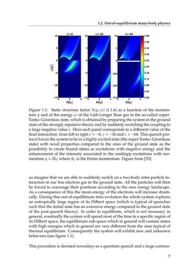
Figure 1.1: Static structure factor S(q , ω) (1.1.6) as a function of the momen-tum q and of the energy ω of the Lieb-Liniger Bose gas in the so-called super-Tonks–Girardeau state, which is obtained by preparing the system in the groundstate of the strongly repulsive theory and by suddenly switching the coupling toa large negative value c. Here each panel corresponds to a dierent value of thenal interaction: from left to right c −8, c −16 and c −64. This quench pro-tocol forces the system to be in a highly excited state (the super-Tonks–Girardeaustate) with novel properties compared to the ones of the ground state as thepossibility to create bound states as excitations with negative energy and theenhancement of the intensity associated to the umklapp excitations with mo-mentum q 2kF where kF is the Fermi momentum. Figure from [33].
us imagine that we are able to suddenly switch on a two-body inter-particle in-teraction in our free electron gas in the ground state. All the particles will thenbe forced to rearrange their positions according to the new energy landscape.As a consequence of this the mean energy of the electrons will increase drasti-cally. During this out-of-equilibrium time evolution the whole system exploresan entropically large region of its Hilbert space (which is typical of quenchessuch that the initial state has an extensive energy compared to the ground stateof the post-quench theory). In order to equilibrate, which is not necessary ingeneral, eventually the systemwill spendmost of the time in a specic region ofits Hilbert space, the equilibrium sub-space which in general will contain stateswith high energies which in general are very dierent from the ones typical ofthermal equilibrium. Consequently the system will exhibit new and unknownbehaviors (see gure 1.1).
This procedure is denoted nowadays as a quantum quench and a large commu-
7
1. Introduction
nity of physicists is involved in understanding how many-body quantum sys-tems behave under these circumstances. A quench consists in preparing thesystem in a pure state |Ψ0〉 usually an eigenstate of a certain Hamiltonian H0,and then to let it evolve with a dierent Hamiltonian H which clearly does notcommute with H0 [34–36] (for some of the major experimental realizations of aquantum quench see [37–45]). The time evolution is unitary and can be writtenin terms of the eigenstates |α〉 of the nal Hamiltonian H
|Ψ0(t)〉 e−iHt|Ψ0〉
∑α
〈α |Ψ0〉e−itEα |α〉 . (1.2.2)
One may naively think that a system undergoing unitary time evolution nevershows any sign of relaxation or equilibration. This is clearly true for the densitymatrix of the state |Ψ0(t)〉〈Ψ0(t) |, whose matrix elements keep oscillating withfrequencies determined by the many-body spectrum Eα. However the out-of-equilibrium behavior is largely dierent when looked at from the point of viewof local observables. Indeed a local observables, like for example themomentumdistribution of a single particle of a gas of N particles in a volume L, probesonly a thermodynamically vanishing sub-region of the whole system. Thereforewe may expect that the rest of the system acts as a bath, leading to an eectiveequilibrium state from the point of view of expectation values of local operatorsO(x) acting on the sub-region [x , x + δx] for any x
limt→∞
limth〈Ψ0(t) |O |Ψ0(t)〉 〈O〉eq (1.2.3)
where the thermodynamic limit limth at xed density n N/L has to be takenrst in order to avoid quantum recurrences for large times and we imposedlimth δx/L 0. The questions of how to characterize 〈O〉eq as a function of theoperator, the initial state and the model with Hamiltonian H driving the timeevolution, together with the time scales for the approach to the equilibrium aswell as the full dynamics towards it constitute a big challenge of modern dayphysics. The answers to those questions would clarify the mechanisms guid-ing the out-of-equilibrium relaxation of interacting quantum particles when iso-lated. In this case we are not entitled to simply rely on the usual Gibbs assump-tions for the equilibration of the system and we are in position to determinethe cases where the system does not thermalize in a standard Gibbs way. Wecan then address the emergence of macroscopic statistical properties of many-body systems from their microscopic interactions which, unlike in the classi-cal case, remains up to now an open big question of fundamental importancethroughout physics, in elds ranging from cosmology [46] and superuid he-lium [47], heavy-ion collisions [48] all the way to atomic-scale isolated quantumsystems [36].
The question of howequilibration ormore specically thermalisation can emergefrom the unitary time evolution of equation (1.2.2) goes back to the very origins
8
1.2. Out-of-equilibrium many-body physics
of quantum mechanics. It lead John von Neumann (1903-1957) to formulate hisQuantum Ergodic Theorem [49]. Here von Neumann tries to establish a connec-tion between the idea of ergodicity in classical mechanics with the analogousquantum mechanical one. In classical physics, given an initial states X0 in thephase space of the model, the time average over the position of the state X0(t)under Hamiltonian time evolution corresponds to the microcanonical averagewith uniform measure on the energy surface dµmc δ(EX − EX0 )dX over thephase space. This is true for most initial state X0, in other words, up to a mea-sure zero set in the Lebesgue measure over the phase space. In order for thesame to be true in quantum mechanics it would require that given the initialstate |Ψ0〉 with energy E0 〈Ψ0 |H |Ψ0〉 and the time average of its density ma-trix given by |Ψ0(t)〉〈Ψ0(t) |
∑α |〈α |Ψ0〉|
2|α〉〈α | then the following should be
valid
|Ψ0(t)〉〈Ψ0(t) | ∑α
|〈α |Ψ0〉|2|α〉〈α |
1D(E0)
∑α:Eα∼E0
|α〉〈α | , (1.2.4)
where D(E0) ∑α:Eα∼E0 1 is the dimension of the sub-space spanned by eigen-
states with energy E0 up to nite size deviations. Equation (1.2.4) is clearly nottrue for any initial state. However von Neumann proves that provided we candecompose the Hilbert space into a set of sub-spaces Hν where a set of mu-tually commuting observables Ak have all the same expectation values dαν forall the states in the macrostateHν up to nite size corrections, then the densitymatrix on the left ismacroscopically equivalent to the one of the right, namely forany Ak and in the thermodynamic limit the following holds
Tr(Ak |Ψ0(t)〉〈Ψ0(t) |
)∼
1D(E0)
Tr *.,Ak
∑α:Eα∼E0
|α〉〈α |+/-
(1.2.5)
However the theorem does not specify how to construct the macroscopic oper-ators Ak and it is therefore not clear how to connect them with the physicaloperators corresponding to the observables we can see in the lab. As shownin [50] the theorem is valid for most decompositions Hν and therefore for mostHamiltonians H (and all the operators we can construct with their eigenstates).However the idea of most is based on an average over the ensemble of randomHamiltonians connected by unitary uniformly distributed matrix H′ UHU−1
(the uniform probability distribution over the unitary group is known as theHaar measure). If a propriety is true for most Hamiltonians it means that it failsonly for some in a zero-measure set. This method of averaging over all possiblerealizations belongs to a long tradition which includes also Wigner’s work onrandom matrices [51]. It relies on the a-priori assumption that the vast majorityof the elements in the ensemble share the same properties. WhileWigner’s workfocused on non-local Hamiltonians describing the interactions inside the atomicnuclei, the physical Hamiltonians for realizable condensed matter systems are
9

1. Introduction
expected to be strictly local and therefore to form a subleading measure set un-der the Haar measure.
An analogous approach to thermalisation in quantum system is provided bythe so called Eigenstate Thermalisation Hypothesis (ETH) [52,53]. It states that,given a few-body observable O (namely a local observable as dened before),in the thermodynamic limit its diagonal elements on the basis of eigenstatesOαα 〈α |O |α〉 change slowly with the choice of the eigenstate |α〉 and that theo-diagonal elements Oαβ 〈α |O |β〉 with Eα , Eβ, are exponentially small inthe system size N (where N is the number of particles in the system). Giventhese two generic hypotheses one can easily see that the time average of the ex-pectation value of the operator O converges to the microcanonical distributiongiven an eigenstate |αE0〉 with energy E0
〈Ψ0(t) |O |Ψ0(t)〉 ≡ limT→∞
1T
ˆ T
0dt 〈Ψ0(t) |O |Ψ0(t)〉
∑α
〈α |O |α〉|〈α |Ψ0〉|2∼ 〈αE0 |O |αE0〉
∑α
|〈α |Ψ0〉|2
〈αE0 |O |αE0〉 , (1.2.6)
where we considered a non-degenerate spectrum Eα , Eβ for |α〉 , |β〉 andoverlaps |〈α |Ψ0〉|
2 which are suciently sharp around the energy E0 of the ini-tial state. This corresponds to choosing initial states which satisfy the clusterdecomposition principle such that the energy uctuations are subleading
∆EL
√〈Ψ0 |H2 |Ψ0〉 − 〈Ψ0 |H |Ψ0〉2
L∼ L−1/2 , (1.2.7)
which is a typical feature of physically relevant states. We can easily see thatthe two hypotheses both depend strongly on the locality of the Hamiltonian inthe Hilbert space (in contrast with the locality in the real space). To be moreclear, let us choose a spin model and its local spin basis. Let us consider theone-dimensional Ising model
HI ∆
N∑j1σz
j σzj+1 , (1.2.8)
where we impose period boundary conditions. TheHamiltonian HI is diagonal-ized by the local spin basis |σ1 . . . σN〉 where σi ±1. Therefore the expectationvalue of a simple local observable as O σ+N/2σ
−
N/2+1 is highly discontinuous(it can be 1,0,-1 just choosing eigenstates with dierent spin σN/2). Therefore aHamiltonian as HI cannot be expected to satisfy the requirements of ETH. We
10

1.3. Out-of-equilibrium integrable models
can then consider adding terms to HI that make it to be less diagonal in thisbasis. This for example can be done by adding a simple hopping term
HXXZ JN∑
j1
(σ+j σ
−
j+1 + σ−
j σ+j+1
)+ ∆
N∑j1σz
j σzj+1 . (1.2.9)
In this case the Hamiltonian is not exactly diagonalized by the local spin basis|σ1 . . . σN〉. We can therefore expect that the expectation value of the operatorO σ+N/2σ
−
N/2+1 is now a smoother function of the eigenstates of the system. In-troducing less local terms that force the eigenstates to involve more local spinstates (like a next-neighbors interaction
∑Nj1 σ
zj σ
zj+2) can only make the expecta-
tion values even smoother. We can try to formalize this argument by introducinga mapping between the basis of eigenstates and the local spin basis
|Eα〉 ∑
σ1±1,...,σN±1cασ1 ,...,σN
|σ1 , . . . , σN〉 . (1.2.10)
With such a mapping we can argue that depending on the spread of the co-ecients cασ1 ,...,σN
(or alternatively on the Shannon entropy associated to them)we can expect dierent type of equilibration according to the ETH. Free mod-els are clearly the simplest case where the sum involves only one term, inte-grable models have non-trivial coecients cασ1 ,...,σN
for each eigenstate but stillin a way that there is some notion of locality in their eigenstates (the Hamilto-nian of an integrable model commutes with N local operators). Perturbing thesystem away from integrable points clearly brings more non-zero terms in thesum (1.2.10), eventually leading to smooth expectation values of local operatorsOαα ∼ Oα+1α+1. It is not clear if the transition between the two behaviors, in-tegrable and non-integrable is smooth or discontinuous although it is hard toimagine the coecients in the sum (1.2.10) to not be smooth functions in thespace of possible Hamiltonians (some evidences of this fact are provided forsystems with nite size in [54–58]). This is also supported by some analysis ofthe local conserved quantities of a perturbed integrable system (see the next sec-tion 1.3). While the transition between integrable and non-integrable systems,and therefore between ergodic and non-ergodic systems, is well understood inclassical physics (the KAM theorem gives quantitative predictions for the break-ing of classical integrability under nonlinear perturbations, see next section), inquantum mechanics it still remains an unsolved problem.
1.3 Out-of-equilibrium integrable modelsIn the summer of 1953 Enrico Fermi, together with John Pasta, Stanislaw Ulam,and Mary Tsingou numerically simulated a chain of N atoms coupled by an-harmonic strings (FPU problem). Given the displacements x j (t) for any j
1, . . . ,N from the equilibrium positions, the equations of motions for the system
11

1. Introduction
were given by
∂x j
∂t
(x j+1 + x j−1 − 2x j
a2
) (1 + α(x j+1 + x j−1)
)j 1, . . . ,N , (1.3.1)
with some α , 0, period boundary conditions and lattice spacing given by a.Starting from a certain initial conguration x j (0)Nj1 the system was believedto ergodically explore during time all its phase-space and to eventually ther-malise in a canonical way, leading to a stationary state where each oscillatorymode ωk
Nk1 had the same energy (according to the Equipartition Theorem).
However even for long times after the start of the simulation, the system kepta complicated quasi-periodic behavior, where localized non-dispersive waveswere traveling through it. Only after 10 years it became clear that these solitonwaves [59] were solutions of the Korteweg–de Vries equation, representing thecontinuous limit α → 0, a → 0, δ lim
√a/(24α) with x j (t) → u(x , t) of (1.3.1)
∂2u(ξ, τ)∂ξ∂τ
−∂u(ξ, τ)∂ξ
∂2u(ξ, τ)∂ξ2
− δ2∂4u(ξ, τ)∂ξ4
, (1.3.2)
where ξ x − t and τ tα/a. This equation represents one of the classicalintegrable systems, namely it has a denumerable innity of integrals of mo-tion Pn that constrain the trajectory in phase-space on hyper-tori, leading to anon-ergodic behavior. The surprising fact is that a system as the one character-ized by equations (1.3.1) exhibits most of the features of an integrable system(1.3.2), despite the integrability breaking given by the lattice spacing a. This ap-parent paradox was solved between 1962 and 1963 when Vladimir Arnold andJürgen Moser proved the so-called Kolmogorov–Arnold–Moser theorem [60].This roughly states that if an integrable system is subjected to a weak nonlinearperturbation, some of the invariant tori in the phase-space are deformed andsurvive, while others are destroyed. This implies that the motion continues tobe quasiperiodic, with the independent periods changed (as a consequence ofthe non-degeneracy condition). Moreover the KAM theorem species quantita-tively what level of perturbation can be applied for this to be true.
The equivalent of the FPU problem in quantum mechanics was given only re-cently. In an experiment known as a quantum Newton’s cradle, a gas of point-wise interacting cold atoms is prepared in a one-dimensional tube [37]. Then att 0 two Bragg pulses distribute the gas in two separate cloudsmovingwith op-posite momenta. As time passes, due to the parabolic conning the two cloudsscatter many times but the distribution of momenta n (t) (k) of the atoms neverrelaxes to a thermal distribution nT (k) with some eective temperature T. Onthe contrary, it keeps memory of the initial splitting of the momenta for verylarge times. This experiment showed that a one-dimensional gas with point in-teractions, despite the integrability breaking perturbation induced by the har-monic conning, displays most of the features of a quantum integrable model,
12
1.3. Out-of-equilibrium integrable models
namely the Lieb-Liniger gas of δ−interacting bosons 6. It became then evidentthat quantum integrablility, at least in some conditions, is also as stable as itsclassical counterpart.Many eectively one-dimensional models that can be realized in a laboratoryare very close to quantum integrable systems. That is why studying the out-of-equilibrium dynamics in integrable models has two great advantages: it pro-vides a platform from which to understand how local interactions lead to ther-malisation in a many-body quantum system and it gives solid predictions forsystems that we can realize in laboratories around the globe.
A quite widespread misconception is that if a model is integrable, then it is ex-actly solvable and therefore it is trivial to compute any of its properties. This isfar from being true, especially for interacting integrable models. The non-linearmapping between the basis of local operators Ak and the one of given by theenergy eigenstate makes the problem of computing even a single diagonal sumas
〈Ψ0(t) |Ak |Ψ0(t)〉 ∑α
〈α |Ak |α〉|〈α |Ψ0〉|2 , (1.3.3)
a very hard one, especially in the thermodynamic limit. Therefore a numberof hypotheses have been formulated to simplify the problem of computing thenon-equilibrium expectation values of local observables. The main ones, whichare also heavily used in this work, are the Generalized Gibbs Ensemble (GGE)and the quench action (QA) method. The rst one relies on the local symme-tries of the system, namely a set of local operators Qn that commute with theHamiltonian giving the time evolution, to determine an eective description ofthe diagonal ensemble |cα |2 [35, 61]. Given a complete set (See section 2.1) oflocal conserved quantities the GGE hypothesis states that in the thermodynamiclimit limth the diagonal ensemble can bewritten as aGibbs densitymatrixwhereall the local conserved quantities are taken into account
limt→∞
limth〈Ψ0(t) |Ak |Ψ0(t)〉 Tr
(Ak e−
∑n βn Qn
). (1.3.4)
This idea, based on the maximal entropy principle, was proven to be true formany free models (where the dynamics is one-particle reducible) [62–70] andLuttinger liquid theories (free bosonic eld theories) [39,71–73]. In the interact-ing cases, the GGE ensemble has been observed numerically in the Lieb-Linigermodel [74] and analytically in the q-boson model [75]. Although it is a very ap-pealing idea its implementation is not straightforward in interacting systems.For an interacting system, where the trace cannot be factorized on a product of
6The lack of thermalisation could also be due to the high relative velocity of the two clouds, lead-ing to a vanishing cross section for the scatterings between the atoms in each of them. Howeverthe same experiment was reproduced in three dimensions, where canonical thermalisation was ob-served [37].
13

1. Introduction
traces over the single particle state, it is very hard for a generic quench to ex-tract the values of the chemical potential from the expectations of the conservedcharges on the initial state
limth〈Ψ0 |Qm |Ψ0〉 Tr
(Qm e−
∑n βn Qn
)∀m . (1.3.5)
Despite the fact that this problem has been solved in a number of cases [4,66,76],still it is unclear if the methods used in these works can be generalized to dier-ent models. The more serious issue is however the determination of the relevantcharges to put into the ensemble. Indeed to determine if a set of charges Qn
is complete it is a very hard task even for free models [77]. A criteria based onthe locality of the charges seems to be the proper way but some recent resultsshowed that in some cases it is not enough [4, 78] .
The quench action approach ( introduced in [79] and applied in a number ofcases [1,4,6,78,80–83] ) on the other hand instead of involving the internal sym-metries of the system, attempts to rewrite the overlaps into something simplerby taking their thermodynamic limit. For initial states that overlap with an ex-ponential number of eigenststates of the nal Hamiltonian the overlaps are ex-pected to scale exponentially in the system size L
〈α |Ψ0〉 ∼ e−LFα , (1.3.6)
where F ≥ 0 is a smooth function of α that does not therefore depend on thedetails of the eigenstate |α〉 (and not even on the details of the initial state |Ψ0〉).Knowing the function Fα one then calculates the sum in (1.3.3) with a saddlepoint approximation, valid for large system sizes which allows to compute thesum by evaluating it on a saddle point state
limt→∞
limth〈Ψ0(t) |Ak |Ψ0(t)〉 〈αsp |Ak |αsp〉 (1.3.7)
analogously to the thermalisation mechanism predicted by the ETH (1.2.6). Themain diculty in this approach is to determine the function Fα. Up to now it ispossible only by knowing the exact overlaps for a generic system size and thentaking their thermodynamic limit. Clearly this is a quite dicult procedure inmany cases since the overlaps are not explicitly known in most cases and theirnite size expressions are in general complicated. However one can imagine todevelop a method to extract the function Fα given a certain initial state withoutthe knowledge of the exact overlaps at nite size. This clearly can also be donewith the help of the conserved quantities of the systemwhich impose constraintson the overlaps.
Another consequence of the quench action approach is the possibility of extract-ing the time evolution towards the steady state which is a very complicated non-linear problem for an interacting system. This is given in terms of eigenstates
14

1.3. Out-of-equilibrium integrable models
which are very close to the saddle point state
limth〈Ψ0(t) |Ak |Ψ0(t)〉
12
∑β∼αsp
cβcsp
e−it(Eβ−Eαsp )〈αsp |Ak |β〉
+c∗βcsp
e it(Eβ−Eαsp )〈β |Ak |αsp〉 . (1.3.8)
This expression allows to reconstruct thewhole post-quench time evolution start-ing from their t ∞ limit which corresponds to the steady state expectationvalue. Therefore it shows that the main features of the whole time evolutionfrom t 0+ after the quench are inuenced by the saddle point state whosestructure does not only provide the physics of the system for innite time afterthe quench. As shown in [80] it can directly provide the maximal propagationvelocity of the excitations in the system after the quench. It is well known indeedthat in a lattice system, given a two-point correlation function at distance `, thereis a maximal velocity v such that a characteristic time t∗ `/v is needed in orderto observe a non-zero dynamical correlation between the two observables A, Bwith nite support placed at distance `
〈[A(x + `, t), B(x , 0)]〉 < const × e−`+v |t | . (1.3.9)
This expression is known as the Lieb-Robinson bound [84] and it has been testedexperimentally for the rst time by studying the non-equilibrium dynamics ofa quantum system in [40]. It only infers the existence of the maximal velocity vbut it does not give any way to nd it. In general it will be a function of the aver-aging state. For free fermions on a lattice therefore will be simply given by theirFermi velocity v vF
√2mεF . The quench action approach also tells us that
when the averaging state is not an eigenstate of the system, namely the initialstate |Ψ0〉, there exists a maximal velocity vsp given by the maximal derivativeof the dispersion relation for the low-lying excitations around the saddle pointstate. Note that vsp is an explicit function of the saddle point state which is de-pendent on the initial state |Ψ0〉. Dierent initial states therefore would lead toa light-cone propagation of excitations with a velocity which in general is verydierent from the Fermi velocity.
Another consequence of formula (1.3.8) is that it allows to easily extract the timedependence when time is large but not innity. Then in this case the relevantstates around the saddle point restrict to a much smaller subset. These are ob-tained by performing simple particle-hole excitations on the saddle point state|αsp〉 → |αsp , h → p〉, i.e. to displace one quasi-momenta from the set whichparametrizes the saddle point state from its original value h to a new value p.These type of excitations have a dispersion relation for the particle εp ω(p)and one for the hole εh −ω(h). Analogously they have an overlap with re-spect to the saddle point state for the particle c(p) and one for the hole 1/c(h)
15
1. Introduction
and a density of states ρh (p) and ρ(h) which are all functions of the saddle pointstate |αsp〉. Therefore we can rewrite the time evolution for large times as a sumover these types of excitations
limth〈Ψ0 |Ak |Ψ0〉 ∼ 〈αsp |Ak |αsp〉+
12
ˆ∞
−∞
dp ρh (p)ˆ∞
−∞
dh ρ(h)c(p)c(h)
e−itω(p)+itω(h)〈αsp |Ak |αsp , h → p〉
+ 12
ˆ∞
−∞
dp ρh (p)ˆ∞
−∞
dh ρ(h)c∗(p)c∗(h)
e itω(p)−itω(h)〈αsp , h → p |Ak |αsp〉
(1.3.10)
The integral can then be evaluated using a stationary phase approximationwhent is large, leading to an expansion in powers of 1/t providing the leading powerlaw for the approach to the steady state
〈Ψ0(t) |Ak |Ψ0(t)〉 − 〈αsp |Ak |αsp〉 ∼ t−γsp . (1.3.11)
It is worth emphasizing that the steady state expectation values of local opera-tors, aswell as the propagation velocity vsp and the leading 1/t exponent γsp , areexpected to be very smooth functions of the initial state. In particular they areexpected to depend on amuch smaller set of information than the one needed toreconstruct its entire initial wave-function Ψ0(x). The GGE hypothesis indeedprovides a saddle point state which is a function only of the very rst conservedquantities Qn (the energy of the initial state and some others) since the sum∑
n βnQn is expected to be absolutely convergent. The velocity vsp and as wellas the exponent γsp are therefore also expected to be dependent on few thermo-dynamic quantities of the system. The question of which conserved charges aremore relevant to reconstruct these quantities is not fully answered yet.
Finally, after having addressed the statistical properties of an integrable system,we may wonder how from integrable models we recover canonical (ergodic)systems. In other words we should expect that if we perturb an integrable sys-temwith a perturbation breaking integrability Vo , the system should thermalizecanonically, namely the late time expectation values of local operators should bedescribed by the Gibbs ensemble
limt→∞
limth〈Ψ0(t) |Ak |Ψ0(t)〉Vo Tr
(e−βHAk
). (1.3.12)
One of the possible questions is if the transition between integrable and non-integrable is smooth (as it is in classical mechanics) or exhibit a certain thresholdin the strength of the perturbation Vo , which separates the two behaviors. Thequestion is not easy since it may depend strongly on the considered observableAk , the initial state |Ψ0〉 and the type of perturbation applied to the integrablesystem. The dependence on the initial state can be indeed particularly strong
16

1.4. Outline of the thesis
as is shown in [85]. Here the authors underline that for initial states suciently"close" to most eigenstates (namely the overlaps are not exponentially vanishingfunctions for large system sizes as in (1.3.6)), the systemkeepsmemory of the ini-tial conditions even when no non-trivial conserved quantities are present. Thisis also the case of a quench in the gapped XXZ model starting from a domainwall initial state [86] which does not exhibit thermalisation due to the nite largeoverlap of the initial state with a macroscopic number of degenerate eigenstatesof the system.Regarding perturbed integrable systems the pre-thermalisation hypothesis statesthat an out-of-equilibrium perturbed integrable model reaches a steady state forintermediate time scales described by a deformed GGE (constructed with con-served quantities forming a mutually commuting set and which do not com-mute with the Hamiltonian) [87] or by a time-dependent GGE [88] (when theunperturbed system has a non-abelian set of local conserved charges) while itthermalize to a canonical Gibbs distribution for larger time scales. Evidences forthis type of behavior have founded theoretically in [87–93] and experimentallyin [94,95]. However some numerical works shows also the existence of an orderparameter separating the integrable and the non-integrable phase of a genericone-dimensional model [96, 97].
1.4 Outline of the thesisThe main purpose of this thesis is to present an exact computation of the oneor two-points correlation functions of integrable models (in particular the Lieb-Liniger model [22] and the XXZ spin chain [98–100]) in equilibrium and nonequilibrium conditions and for large system sizes (thermodynamic limit). Thisis done rst by introducing the fundamental tools of the coordinate and alge-braic Bethe ansatz in chapter 2 which allows to obtain the exact eigenfuntionsand scalar products between them. In this chapter we also address the questionof how to determine when a quantum model is integrable or not, following thework of Jorn Mossel [101, 102]. Then in chapter 3 we move to the problem ofcomputing overlaps between eigenstates of dierent models. This has a directapplication to quench problems and until now it has been poorly addressed inthe eld of integrable systems. Chapter 4 is devoted to an extensive treatment ofthe thermodynamic limit of integrablemodels. In particularwe focus on the ideaof thermodynamic Bethe states, namely how to characterize them and how todene the matrix elements between them, starting from their nite size expres-sions. Herewe obtain some results for equilibriumnite temperature correlationfunctions in the one-dimensional Bose gas, which represent a direct extensionof the work initiated in Miłosz Panl’s thesis [103]. Thereafter we concentrateon the out-of-equilibrium aspects of the Lieb-Liniger model in chapter 5 focus-ing in particular on the quench from the ground state of the free bosonic theory(BEC state) to the fully interacting system. The corresponding post-quench timeevolution of weak observables, computed via the quench action method, is ad-
17
1. Introduction
dressed in chapter 6. Finally chapter 7 analyzes the quench from the Néel initialstate to the XXZ spin chain. This quench reveals unknown results on the con-served quantities of the model, underlining the role of quasi-local operators toreconstruct the equilibrium steady-state values of local operators even when thespectrum of the Hamiltonian is gapped.
18
CHAPTER 2
Integrability and Bethe Ansatz
There is geometry in the humming ofthe strings, there is music in thespacing of the spheres.
Pythagoras, The Mystery of Matter,L. Young
This chapter is devoted to the problem of dening an integrable system andhow to compute its physical properties. The rst is a highly non-trivial questionwhose precise answer is still under investigation. It is well established that in-tegrable systems are characterized by many symmetries, which allow to writedown their exact eigenstates and the scalar products between them. The rstcan be done with the rst quantization approach of the coordinate Bethe ansatzwhile the secondneeds the development of a secondquantization-like approach,the algebraic Bethe ansatz.
We rst introduce the Bethe wave function (section 2.1), which is an exact eigen-states of a model where particles scatter without diraction [104, 105], namelyeach n−body scattering among the constituents of the system can be factorizedin a sequence of 2−body scatterings. We will nd out that this is possible onlyin models that have a number M of conserved operators (where M is the totalnumber of particles). Since these are extensive conserved quantities, in the senseof the scaling with the total number of particles, the Mazur’s inequality (section2.1) suggests that they inuence the out-of-equilibrium dynamics of the system,leading to non-ergodic out-of-equilibrium dynamics.Thenwe shall introduce the twomainmodels considered in this thesis, the Lieb-Liniger model for a gas of δ−interacting bosons, which we diagonalize via thecoordinate Bethe ansatz (section 2.2), and the XXZ spin chain, for which we usethe tool of algebraic Bethe ansatz (section 2.3 and section 3.2.1).
The main concepts and results of this chapter are contained in [105–108] andreferences therein.
19
2. Integrability and Bethe Ansatz
2.1 Quantum Integrability and the Bethe wave func-tion
We consider a one-dimensional physical model of interacting particles. To beconcrete let us restrict ourselves to a spin chain where each site is separated bya distance a 1 and where the down spins are considered as the particles in thetheory. When only few spins are ipped down they are free to travel on the spinchain except when their paths cross. We can make the physical assumption thatthe range of the interaction between them is very small, for example just twosites. Therefore the Hamiltonian is the sum of the kinetic part, associated withthe hopping of the spins in the lattice, and a nearest-neighbors interaction
H
N∑j1
[σ+j σ
−
j+1 + σ−
j σ+j+1
]+
N∑j1
∑k1
U j, j+k , (2.1.1)
with ` N . We then now restrict ourselves to the scattering of only two spins,namelywe take our spin chainwith N−2 spins up and only 2 spins down. Whenthe two spins are spatially separated such that the interacting part of the Hamil-tonian is zero, we can associate to each of them a free momentum ki ∈ [−π, π]where i 1, 2 and their energy will be simply given by the free dispersion rela-tion for particles on a lattice ε(k) cos(k). For simplicity we can consider onlysmallmomenta such that the dispersion relation becomes quadratic ε(k) ∼ 1− k2
2 .After scattering the two spins move freely again but with two new momenta k′iassociated to them (we assume that the Hamiltonian preserves the total spin ofthe system). However by enforcing the conservation of the total momentum andenergy we obtain a complete set of constraints on the two nal momenta
k′1 + k′2 k1 + k2 , (2.1.2)(k′1)2 + (k′2)2 (k1)2 + (k2)2 . (2.1.3)
We can easily argue that the only possibility for the two nal momenta is simplyto be a permutation of their initial values. In quantum mechanical language wecan introduce a wave function ΨOut for the two spins after the scattering withthe following form, given a normalization factorN−1
ΨOut N−1
(e is1k1+is2k2 − e−iθ(k1 ,k2) e is1k2+is2k1
), (2.1.4)
where the index si ∈ [1, . . . ,N], i 1, 2 labels the position of each spin inthe lattice and the wave function is supposed to be exact only in the asymptoticdomain s1 s2 when the two spins are spatially separated again after the scat-tering. Note that we introduced a phase factor in front of the component of thewave function where the two spins have exchanged their momenta. We can in-terpret this classically as a delay in the wave vectors of the two spins due to the
20
2.1. Quantum Integrability and the Bethe wave function
interaction that the two particles feel when they cross each other. We can rewritethe abovewave function in terms of a sumof permutations P ∈ S2 of the set [1, 2]
ΨOut N−1
∑P∈S2
a(P)2∏
i1e isi kPi , (2.1.5)
where a(P) is the phase factor which can be either 1 or −e−iθ(k1 ,k2) in this case.By ipping an extra spinwe nowallow a scattering involving three particles. Themere conservation of the total momentum and energy is not enough to simplycause a rearrangement of the spin momenta among themselves after the scatter-ing. We can however split the nal wave function in a term only due to two-bodyscatterings and a termwhere all the possible waves with newmomenta are pro-duced, the so called diractive term
ΨOut N−1 *.
,
∑P∈S3
a(P)3∏
i1e isi kPi +
3∏i1
[ ˆdki e isi ki
]S(k1 , k2 , k3)+/
-, (2.1.6)
where S(k1 , k2 , k3) is a function related to the interacting part of theHamiltonianand the integration domain is chosen in such away that the total energy andmo-mentum is conserved. Adding more spins to this picture extremely complicatesthe problem due to the diractive part and nding an analytical expression forthe wave function becomes a hopeless task.We can therefore introduce a new assumption on the interaction potential U,namely that it conserves a third extra additive quantity Q3 with eigenvaluesgiven by
∑3i1 q3(ki ). If this is true the set of momenta before and after the scat-
tering, besides energy andmomentum conservation, are now also related by thefollowing equation
3∑i1
q3(ki ) 3∑
i1q3(k′i ) . (2.1.7)
If the function q3(k) is not proportional to a linear combination of k or ε(k) thisis enough to set the diractive part of the wave function to zero. 1 The wavefunction is then only constituted by the part corresponding to only two-bodyscatterings between particles. Keeping the same way of reasoning we can thenintroduce a number M of independent constraints on theHamiltonian andwritedown an exact wave function for M down spins valid in the asymptotic regions1 s2 . . . sM
ΨB (s j Mj1 |k j
Mj1) N−1
∑P∈SM
(−1)[P]M∏
i< j1e−
i2 θ(kPi−kPj )
M∏i1
e isi kPi , (2.1.8)
1A generic symmetric polynomial of the three momenta with degree larger than two would havethe same eect.
21
2. Integrability and Bethe Ansatz
where (−1)[P] is the sign of the permutation P. This is the Bethe wave function orthe coordinate Bethe ansatz wave function and it is an the exact eigenfunctionfor each Hamiltonian like (2.1.1) with a short range interaction (such that ` 1,with the asymptotic region given by s1 < s2 < . . . < sM) that supports non-diractive scattering, or such that it commutes with a number M − 1, with Mthe total number of constituents in the system, of linearly independent, additiveconserved quantities. If we impose a certain boundary condition (for examplethe period boundary conditionsΨB (x j
Mj1 |k j
Mj1) ΨB (x j + δ j,l N Mj1 |k j
Mj1)
with l 1, . . . ,M) then the set of quasi-momenta k j Mj1 satises a set of non-
linear coupled equations named Bethe equations which have the following form(for period boundary conditions)
e iNkl (−1)M−1∏i,l
e−iθ(kl ,ki ) , l 1, . . . ,M . (2.1.9)
When the set k j Mj1 satises such conditions, the state |k j
Mj1〉 is aBethe state and
all the possible choices of the quasi-momenta k j Mj1 form a complete basis of the
Hilbert space. The set of M conserved operators Qn Mn1, where we included the
Hamiltonian and the momentum operator, have the Bethe states as eigenvectors
Qm |k j Mj1〉
*.,
M∑j1
qm (k j )+/-|k j
Mj1〉 , (2.1.10)
and therefore they all commute among each other. From the single-particlestructure of the eigenvalues we can notice that when the number of particles Min the system grows, then the eigenvalues grows proportionally to the numberM when this is large enough
M∑j1
qm (k j ) ∼ M . (2.1.11)
We then denote the operators Qn as an extensive operators, referring to the ex-tensivity of their eigenvalues in the particle number M.
We can therefore conclude that in order for the system to have Bethe wave func-tions as eigenfunctions there must be at least a number M of extensive operatorsthat commute among themselves (in order to be diagonalized by the same basisof Bethe wave functions)
[Qm ,Qn] 0 ∀ m , n 1, . . . ,M . (2.1.12)
andwhere theHamiltonian is proportional to one of them (for example H ∝ Q2).We dene such a model as integrable. Note that the presence of the “at least”in
22
2.1. Quantum Integrability and the Bethe wave function
this denition makes it very imprecise. Mainly because we are not specifyingall the conserved operators in the models. There could be more of them indeed,extensive or not. In the next sectionwewill see that for any integrablemodelswecan introduce a generating function τ(λ) (which is an operator on the Hilbertspace of the system) such that the coecients of it logarithmic Laurent seriesgive a set of M extensive conserved charges (see (2.3.22))
[τ(λ), τ(µ)] 0 ∀λ, µ ∈ C , (2.1.13)
log τ(λ) ∑n1
cnQn(λ − λ0)n
n! such that Q2 ∝ H . (2.1.14)
These operators are indeed the ones enforcing integrability. Their extensivity ismanifest also from their representation in a local spin basis as an extensive sumof local spin operators q (n)
j
Qn
N∑j1
q (n)j , (2.1.15)
where q (n)j is a an operator acting non-trivially only on a number r(n) N of
lattice points around j. This set of operators is enough to dene integrability inthe sense of non-diractive scattering but can easily imagine that there are moreconserved charges for the model. We can indeed think to be able to analyticallycontinue the operator τ(λ) in all the complex plane, where, depending on theanalytical properties of τ(λ) there may be other Laurent series for f (τ(λ)) gen-erating new conserved charges for dierent points λ0 in the complex plane anddierent choices of the function f (x).
A full denition of integrability which has reached a general consensus is stillmissing. In the past years there have been several proposals [101, 102](and ref-erence therein). In order to summarize let us say that we can always think in-tegrable quantum models as theories where the evolution is reducible to a two-particles description. Like non-interacting theories are reducible to single par-ticle physics, integrable models are a step forward into the realm of interactingmodels. The question of determining their full symmetry contents is not merelyacademic. As usual in theoretical physics symmetries are extremely helpful tocharacterize the system (and to compute physically relevant results in a muchmore straightforward way). In particular in this case they help us understand-ing the non-equilibrium aspects of the model, which is a complicated non-linearproblem.
Extensivity and Mazur’s inequalityWe can establish a precise connection between the ergodicity of an operator (i.e.an observable) in a quantum theory and the conserved charges present in the
23
2. Integrability and Bethe Ansatz
system. The way of addressing it is still in some sense related to equilibriumphysics. We consider a lattice quantum system in a certain ensemble of states,like the canonical ensemble, specied by some density matrix ρ. Let us consideran operator A which is an extensive sum of local operators
O
N∑j1
a j , (2.1.16)
where a j is an operator with support on the lattice position j and some nitenumber of its neighbours. For example it could be the spin current operator
O iN∑
j1
[σ+j σ
−
j+1 − σ−
j σ+j+1
]. (2.1.17)
We perturb the system out of equilibrium by inserting the operator O at timet 0 and we measure what is the reaction of the system after some time t. Weare therefore interested in the correlation function
〈O(t)O(0)〉N
1N
Tr[ρO(t)O(0)]Tr[ρ] , (2.1.18)
where we included the factor 1N in order to obtain a nite number for the corre-
lation function in the thermodynamic limit. If the operator is ergodic the corre-lation function should oscillate around its average such that
limT→∞
1T
ˆ T
0dt〈O(t)O(0)〉
N〈O〉2
N. (2.1.19)
If it is not ergodic the expectation value relaxes to something that keepsmemoryof the initial conditions at t 0
limT→∞
1T
ˆ T
0dt〈∆O(t)∆O(0)〉
N> 0 , (2.1.20)
where we have dened ∆O O − 〈O〉. The Mazur’s inequality [109–111] statesthat given a set of mutually orthogonal conserved charges Qn
MQ
n1 in the system,the long time average of the correlation function is given by
limT→∞
1T
ˆ T
0dt〈∆O(t)∆O(0)〉
N≥
MQ∑n1
|〈(∆O)Qn〉|2
N 〈QnQn〉, (2.1.21)
where the orthogonality condition corresponds to
〈QnQm〉 δnm 〈QnQn〉 . (2.1.22)
24

2.1. Quantum Integrability and the Bethe wave function
From the rst equation we understand the relevance of extensivity for a con-served charge to non-trivially inuence the ergodicity of an operator. Since theoperator O is given by an extensive sum of local operators, its overlap with anyother operators can only be extensive (at least in for all the density matrices ρthat admit cluster decomposition), therefore
|〈(∆O)Qn〉|2∼ N2 . (2.1.23)
We now see that in order to contribute to a nite Mazur’s bound, the conservedcharge Qn has to be extensive, namely, when the system size N is large (and thenumber of particles M is proportional to it) the expectation value of the chargeis proportional to N
〈QnQn〉 ∼ N . (2.1.24)
This property is clearly valid for the rst o(N) extensive operators introducedin (2.1.13), where o(N)/N → 0 for large N . We can indeed take a at densitymatrix ρ 1 (corresponding to an innite temperature Gibbs ensemble) in theHilbert spaceH and show that, in a spin basis |σ〉 we have
〈QnQn〉 Tr[QnQn]
Tr[1] 1
dimH
dimH∑σ
N∑k1
N∑j1〈σ | q (n)
j q (n)k |σ〉 ∝ N . (2.1.25)
The scaling with N is supposed to be the same for more complex density ma-trices ρ. Therefore one would be tempted to say that the rst o(N) extensiveoperators given by (2.1.13) are the ones enforcing integrability in the system,hence they are the only ones which constrain non-trivially the non-equilibriumdynamics of local observables.However recently it has been showed [112–114] that there exist also conservedcharges of the form
Zn
N∑j1
N∑k1
z (n)j,k (2.1.26)
which satisfy (2.1.24) and are therefore extensive . The sum over the index know spans a range proportional to the system size N but the norm of the op-erators z (n)
j,k are proportional to exponential decaying functions in the extent k
z (n)j,k ∼ e−α(n)k or a power law z (n)
j,k ∼1
kα(n) . Charges with such a structure arecalled quasi-local and how to fully characterize them for a generic integrablemodel is still an open question.
In conclusion we have shown that according to Mazur’s inequality only exten-sive conserved charges, in the sense of (2.1.24), are able to aect the ergodicity of
25
2. Integrability and Bethe Ansatz
physical operators. The rst M (where M is the number of particles in the sys-tem) conserved charges of an integrable system have this property and thereforeare expected to inuence the out-of-equilibrium physics of the model. Howeverit is unreasonable to expect that these are the only extensive conserved chargespresent in an integrable system and there may be others able to inuence thephysics of the model.
Extensivity and dynamics far from equilibrium: GGEMazur’s inequality gives a necessary condition for a certain local observable tonot fully relax after having been perturbed away from its equilibrium value.However it is an analysis based on the linear response of a system in equilib-rium. We are interested however in a full out-of-equilibrium dynamics, as theone given by a quantum quench. In this case, given an initial state |Ψ0〉 of theHamiltonian and given a local operator O, we are interested in the long timelimit of its expectation value in the thermodynamic limit
〈O〉eq limt→∞
limth〈Ψ0 |e iHt Oe−iHt
|Ψ0〉 , (2.1.27)
where the order of the two limits cannot (at least in general) be exchanged. In or-der to study the properties of local operators it is useful to introduce the densitymatrix of the problem
ρ(t) |Ψ0(t)〉〈Ψ0(t) | . (2.1.28)
Let us now assume that we are interested only in operators O with support in-side a region C such that its volume is much smaller than the whole system size|C | N . Therefore we can consider the reduced density matrix ρC (t)
ρC (t) TrC[ρ(t)] , (2.1.29)
where C is the complementary region of C. The time evolution after the quenchof an operator in C it is given by its expectation value on the density matrixρC (t) and in particular the long time limit of the expectation values of all thelocal operators in C is given by the statistical ensemble
ρeq ,C limt→∞
limN→∞
ρC (t) . (2.1.30)
The density matrix ρeq ,C is a local operator since it has support only in C. There-fore one can argue that it must be inuenced only by local data of the initialstate |Ψ0〉 (like the energy density for example). The Generalized Gibbs En-semble (GGE) idea (see section 1.3) is based on the hypothesis that the densitymatrix ρeq ,C in the limit of a large volume |C | → ∞ for the region C, is theone which maximizes the entanglement entropy of the sub-system C, given by−Tr[ρeq ,C log ρeq ,C] under the constraints of a complete set of local charges [67]
26
2.2. Coordinate Bethe ansatz for the Lieb-Liniger model
2 . This is explicit by solving the equation
δδρ
[−Tr[ρ log ρ] − Tr[ρ∑
n
βnQn]ρeq ,C 0 , (2.1.31)
where the set βn is the set of Lagrange multipliers enforcing the constraintsgiven by the local charges Qn . Equation (2.1.31) is solved by
lim|C |→∞
ρeq ,C e−
∑n βn Qn
Tr[e−∑
n βn Qn ]. (2.1.32)
An open question is still how to determine a general criteria to choose the rightset of charges Qn n to construct a proper GGE ensemble for any type of quench.Since the entanglement entropy of the sub-system is expected to grow as N forlarge system size (this is usually the case for initial states |Ψ0〉 that are not tooclose to the ground state or the most excited state of the system), we can expectthat only an extensive operator Q such that
Tr[ρ Q]Tr[ρ] ∼ N (∀ρ : Tr[ρ] < ∞) , (2.1.33)
can represent a non-trivial constraints for the entanglement entropy. Thereforewe can expect that any operator satisfying (2.1.24) has to be included in the GGEdensitymatrix. This is the case of the rst o(N) operators enforcing integrabilityfrom (2.1.13) but also the quasi-local operators of the form (2.1.26). Themaximalset of local charges is therefore expected to contain all of them with no knownprinciple telling us the order of relevance. Only for free models (transverse eldIsing model) there have been a proposal to use its degree of locality in space asa criteria to set the relevance of the conserved charge [67].
A rigorous proof of the validity of the GGE ensemble in free models, after aquench from any initial state |Ψ0〉 satisfying cluster decomposition, namely suchthat, for any operators with nite support A and B
lim`→∞
(〈Ψ0 |A(x)B(x + `) |Ψ0〉 − 〈Ψ0 |A(x) |Ψ0〉〈Ψ0 |B(x + `) |Ψ0〉) 0 , (2.1.34)
has been formulated in [73]. An analogous proof valid for interacting integrablemodel has not been found yet.
2.2 CoordinateBethe ansatz for theLieb-LinigermodelWe now introduce one of the most important integrable model (both from thetheoretical and experimental point of view), the Lieb-Liniger model for a gas of
2A complete set of charges Qn Mn1 is such that given a Bethe state (or also a free-particle state)
|k j Mj1〉 we can uniquely determine the values of all its quasi-momenta k j
Mj1 by computing the
expectation values of all the charges in the state itself 〈k j Mj1 |Qn |k j
Mj1〉
Mn1.
27
2. Integrability and Bethe Ansatz
interacting bosons. The model is diagonalized by Bethe states as in 2.1.8 and thewhole process of nding its eigenstates is denoted as coordinate Bethe ansatz.
Let us introduce the canonical quantum Bose eldΨ(x) with canonical equal-time commutation relations
[Ψ(x),Ψ†(x)] δ(x − y) , (2.2.1)[Ψ(x),Ψ(x)] [Ψ†(x),Ψ†(x)] 0 . (2.2.2)
With this notation we can introduce the Hamiltonian of a Bose gas with pointcontact interaction (for a discussion on the justications for this type of potentialfrom more realistic potentials see [115,116])
H
ˆdx
(∂xΨ
†(x)∂xΨ(x) + cΨ†(x)Ψ†(x)Ψ(x)Ψ(x)). (2.2.3)
The number of particles operator Q0 and themomentumoperator P are integralsof motion and they read as
Q0
ˆdxΨ†(x)Ψ(x) , (2.2.4)
P −i2
ˆdx
(Ψ†(x)∂xΨ(x) − [∂xΨ
†(x)]Ψ(x)). (2.2.5)
Therefore we can now look for a basis of eigenstates Ψ(x) of H, P and Q0 butrst is more convenient to write the Hamiltonian and the momentum operatorin the rst-quantization form
H −
N∑j1
∂2
∂x2j
+ 2c∑
1≤i< j≤N
δ(xi − x j ) , (2.2.6)
P
N∑j1−i
∂∂x j
. (2.2.7)
We want to show that the eigesntates of the Hamitonian (2.2.6) are exactly givenby Bethewave functions (2.1.8). Thiswas rst solved by E.H. Lieb andW. Linigerin [22]. We shall show theway of addressing the problem for a restricted numberN 2 of particles. We write the generic eigenstate by devidng the real line intox1 < x2 and x1 > x2 sectors
Ψ(x1 , x2) Θ(x2 − x1) f (x1 , x2) +Θ(x1 − x2) f (x2 , x1) , (2.2.8)
where we imposed bosonic symmetry on the wave function and where Θ(x)denotes the usualHeaviside step function. We now impose a freewave functionssuperposition as an ansatz on the function f (x1 , x2). This is clearlymotivated by
28
2.2. Coordinate Bethe ansatz for the Lieb-Liniger model
noticing that in the regions x1 < x2 and x2 < x1 the particles are non-interacting
f (x1 , x2) A12e ix1λ1+ix2λ2 + A21e ix1λ2+ix2λ1 (2.2.9)
We now let the Hamiltonian (2.2.6) acting on this ansatz using ∂xΘ(x) δ(x)and f (x)∂xδ(x) −δ(x)∂x f (x) (valid under integral). For the kinetic part weobtain
∂2x1Ψ(x1 , x2) ∂2x1 f (x1 , x2)Θ(x2 − x1) + ∂2x1 f (x2 , x1)Θ(x1 − x2)
− ∂x1 f (x1 , x2)δ(x2 − x1) + ∂x1 f (x2 , x1)Θ(x1 − x2) . (2.2.10)
which leads to
HΨ (λ21+λ
22)Ψ+2δ(x1−x2)[c(A12+A21)− i(A12−A21)(λ1−λ2)]e i(λ1+λ2)x1 .
(2.2.11)
ThereforeΨ is an eigenstate if the following constraints on the amplitudesA12 ,A21is satised
A12A21
i(λ1 − λ2) + ci(λ1 − λ2) − c
≡ −e iθ(λ1−λ2) , (2.2.12)
where θ(λ1 − λ2) is the phase shift due to the contact interaction. We have thenproved that the eigenstate for 2 particles are given by Bethe wave functions. Wecan nally write the expression for the exact eigenstate at any N as a function ofthe N rapidites λ λ j
Nj1 [106]
Ψ(x |λ) F[λ]∑
P
e i∑N
j1 x jλPj∏j>k
(1 −
ic sign(x j − xk )λP j − λPk
), (2.2.13)
where
F[λ]
∏Nj>k1(λ j − λk )√
N!∏N
j>k1[(λ j − λk )2 + c2], (2.2.14)
and with the corresponding energy eigenvalue HΨ(λ) E[λ]Ψ(λ) given by
E[λ] N∑
j1λ2
j . (2.2.15)
Up to now the rapidities λ have been treated as free parameters. Imposing peri-odic boundary conditions we obtain a set of constraints for the wave function to
29
2. Integrability and Bethe Ansatz
be periodic. These are the Bethe equations, a set of non-linear coupled equationsfor the λ
e iλ j L −
N∏k1
λ j − λ j + icλ j − λk − c
j 1, . . .N . (2.2.16)
Taking the logarithm on both the sides of the equations we obtain the Betheequations in logarithm form, which allow to x the values of the rapidites λgiven a set of quantum numbers I I j
Nj1, integers for N odd and half-integers
for N even
λ j 2πI j
L+ 1
L
N∑k1
θ(λ j − λk ) j 1, . . .N . (2.2.17)
These equations manifestly show how the momenta (usually denoted as rapidi-ties) λ have not to be seen as free momenta. They correspond to free momentaλ(0)
j 2πI j
L dressed by the eects of the interaction with all the particles in thering. The limit c → ∞ or L → ∞ makes the interaction trivial and indeed werecover the free momenta in those limits (The limit c → ∞ is denoted as Tonk-Girardeau limit as it was rst introduced in [117] to study a gas of hard-corebosons). However the total momentum of the state is independent of the inter-action and is indeed given by
P
N∑j1λ j
N∑j1
2πI j
L. (2.2.18)
C. N. Yang and C. P. Yang proved [118] that there is a one-to-one mapping be-tween the set of all the choices of mutually distinct quantum numbers in (2.2.17)and all the Bethe eigenstates of the model. The states where two (or more) ra-pidities have the same value have a zero wave function and they correspond tochoices of quantum numbers where two (or more) of them are the same.
To summarize, we obtained the exact eigenstates of the Lieb-Liniger Hamilto-nian (2.2.6). These are given by Bethe wave functions as in (2.1.8) and thereforethe model is integrable (there must be more integral of motions than just mo-mentum and total number of particles (2.2.4)). The eigenstates (2.2.13) are exactbut their structure is intricate due to the sum over the permutations of N mo-menta and in order to compute simply their norm, one has to perform a numberN! of integrals. Therefore an alternative approach where the Bethe states canbe written in a second quantization form and some algebraic properties can beused would be much more useful to compute correlation functions. This will bethe content of the next section.
30
2.3. Algebraic Bethe Ansatz
2.3 Algebraic Bethe AnsatzIn the previous section we considered a specic model, we wrote down its ex-act eigenstates that turn out to be given by Bethe wave functions. In general,given a generic one-dimensional model, it is very hard to establish a priori ifthis is diagonalized by Bethe wave functions (2.1.8). The algebraic Bethe ansatzapproaches the problem by doing the reverse process. Given a scattering ma-trix between two particles with some internal degree of freedom, we build thecorresponding model (Hamiltonians) which supports non-diractive scatteringand is diagonalized by Bethe states. Moreover this allows to introduce a sec-ond quantization formalism for the Bethe states: the non-diraction conditionis transformed into a set of commutation relations between operators responsi-ble for particle creation. With such operators we can write down a generic Bethestate as the action of a product of creation operators over a vacuum state and usethe commutation relations to compute their norms and scalar products.
Let us consider the scattering of two spins S 1/2 labeled by index a 1, 2 withmomenta µ and ν. Each spin lives in its Hilbert space Va which for fundamentalspin representation is the space Va C2. The scattering between the two canbe characterized by a scattering matrix Rab : Va × Vb → Va × Vb whose matrixelements correspond to the amplitudes associated to each scattering process forany given conguration of initial spins | ↑↑〉, | ↑↓〉, | ↓↑〉, | ↓↓〉. We restrict hereto scattering processes that preserve the longitudinal spin Sz such that the mostgeneric scattering matrix is given by
Ra ,b (µ, ν) *...,
↑↑ ↑↓ ↓↑ ↓↓
↑↑ 1 0 0 0↑↓ 0 r(µ, ν) t(µ, ν) 0↓↑ 0 t(µ, ν) r(µ, ν) 0↓↓ 0 0 0 1
+///-
×Θ(µ, ν) , (2.3.1)
where we introduced the transmission t and reection r coecient. Note thatthe scattering matrix can be rewritten as a 2× 2 matrix in terms of the Pauli spinmatrices of the two spins τz
a , τ+a , τ
−a where a 1, 2 is the spin index
Ra ,b (µ, ν) Θ(µ, ν)(1 + τz
aτzb
2 + r(λ)1 − τz
aτzb
2 + t(λ)(τ+a τ−
b + τ−a τ+b )). (2.3.2)
When adding a third spin in our system we also need to impose non-diractivescattering such that any scattering process has to be a sequence of two-bodyscatterings. This is clearly possible only if bymaking dierent sequences of two-body collisions we obtain the same nal scattering amplitude. We can enforcethis consistency relation as a set of constraints on the two-body scattering, namelyon on the matrix Ra ,b . This is set of constraints can be written as the Yang-Baxterequation for the R−matrix
R1,2(λ, µ)R1,3(λ, ν)R2,3(µ, ν) R2,3(µ, ν)R1,3(λ, ν)R1,2(λ, µ) . (2.3.3)
31
2. Integrability and Bethe Ansatz
This equation tells that in a scattering of three spins it does not matter whichone is the order of the scattering processes since the nal result is the same. Asolution of this equation is given by the following expression for the coecientsgiven in term of the generic complex parameter η
t(λ, µ) ≡1
f (λ, µ)
sinh(λ − µ)sinh(λ − µ + η)
, (2.3.4)
r(λ, µ) ≡g(λ, µ)f (λ, µ)
sinh(η)
sinh(λ − µ + η). (2.3.5)
(2.3.6)
where we introduced two new functions f (λ, µ) and g(λ, µ) which will turnuseful later. Note that when one of the two momenta is very large λ → ∞ onlythe reection coecient goes to zero while the transmission amplitude becomesunitary. The opposite situation we have it when the two momenta are almostequal, when reection is the only relevant process.Let us now consider not only 2 or 3 spins but an entire spin chain living in theHilbert spaceH which is the tensor product of the Hilbert space for each site
H
N⊗j1Hj , (2.3.7)
whereHj C2. We impose now a non-diractive scattering for all the spins inthe spin chain. The way we do it is simply by injecting an auxiliary spin, whichwe can denote as a ghost, in the spin chain and make it interact with the spin ineach lattice position. We impose that the nal result is a sequence of two-bodyscattering of the ghost with each spin in the chain. Let us then introduce thematrix L j,a : Hj ×Va →Hj ×Va for the scattering of a single external spin witha generic spin in the chain at position j. We denote with λ the momentum of theexternal spin and with ξ j
Nj1 the set of momenta of the spin in the chain 3
L j,a (λ, ξ j ) 1 + τz
aσzj
2 + r(λ, ξ j )1 − τz
aσzj
2 + t(λ, ξ j )(τ+a σ−
j + τ−a σ+j ) , (2.3.8)
where now we use the Pauli matrices σzj , σ
+j , σ
−
j for the spin in the lattice posi-tion j 1, . . . ,N and τz
a , τ+a , τ
−a for the spin of the ghosts. The matrix L j,a is
called Lax operator. We now impose that the scatteringmatrix of the scattering ofthe external spin with all the spins in the chain is simply the product of all thematrices L j,a . We denote this matrix as the Monodromy matrix
Ta (λ) LN,a (λ, ξN ) . . .L1,a (λ, ξN ) (A(λ) B(λ)C(λ) D(λ)
). (2.3.9)
3Althoughwe insist calling λ (and ξ j ) as momentum this is not to be intended as freemomentumand therefore it is not necessarily a real parameter.
32
2.3. Algebraic Bethe Ansatz
Each matrix element of the Monodromy matrix is an operator acting on thewhole spin chain and it encodes the scattering of the auxiliary spin through theentire chain. We can indeed write Ta (λ) as
Ta (λ) 12[A(λ) + D(λ)] + 1
2[A(λ) −D(λ)]τza + B(λ)τ+a + C(λ)τ−a , (2.3.10)
from which we can see that B and C are some spin raising/lowering operatorfor the spin chain since they correspond to the process of injecting the auxiliaryspin with a certain spin and extracting it with the opposite one. Since this alsocorresponds to a spin-ip somewhere in the chain, by choosing as reference stateas the spin-up ferromagnetic state
|0〉 N∏
j1| ↑ j〉 , (2.3.11)
we can create state with M spin down in the chain as multiple actions of theoperator B
|λ j Mj1〉
M∏j1
B(λ j ) |0〉 , (2.3.12)
〈λ j Mj1 | 〈0|
M∏j1
C(λ j ) . (2.3.13)
However we still do not have commutation relations between the operators A,B, C and D and therefore we do not know if the states constructed as in 2.3.12are eigenstates of themodel. We have imposed that the whole scattering processgiven by the Monodromy matrix is a result of two-body scattering but still weneed a consistency relation for each of these scatterings. This translates into aYang-Baxter equation for each Lax operator L j,a where now 2 ghost spins areinvolved
L j,a (λ−ξ j )L j,b (µ−ξ j )Ra ,b (λ−µ) Ra ,b (λ−µ)L j,b (µ−ξ j )L j,a (λ−ξ j ) . (2.3.14)
Repeated use of this equation leads to a Yang-Baxter equation for the Mon-odromy matrix
Ta (λ)Tb (µ) Ra ,b (λ, µ)Tb (µ)Ta (λ)Ra ,b (λ, µ)−1 . (2.3.15)
By comparing the left and the right hand side of the equation above we get a setof 16 commutation relations for the operators A, B, C,D. We write here a few ofthem while the entire list can be found in [106]
A(µ)B(λ) f (µ, λ)B(λ)A(µ) + g(λ, µ)B(µ)A(λ) , (2.3.16)D(µ)B(λ) f (λ, µ)B(λ)D(µ) + g(µ, λ)B(µ)D(λ) , (2.3.17)[C(λ, B(µ)] g(λ, µ)(A(λ)D(µ) − A(µ)D(λ)) . (2.3.18)
33
2. Integrability and Bethe Ansatz
Moreover all the operators commute with themselves, for example
[B(µ), B(λ)] 0 , ∀µ, ν ∈ C . (2.3.19)
Equation (2.3.15) allows also to nally relate theMonodromymatrix to a physicalmodel (in the sense of determining the Hamiltonian explicitly). We denote theTransfer matrix as the trace of the Monodromy matrix over the Hilbert space ofthe auxiliary spin
τ(λ) TrC2 (T (λ)) A(λ) + D(λ) . (2.3.20)
Taking the trace corresponds to considering periodic boundary conditions forthe auxiliary spin, i.e. we are interested only in the scattering processes wherethe auxiliary spin keeps the same direction. Using the cyclic property of thetrace we obtain that transfer matrices with dierent momenta always commute
[τ(λ), τ(µ)] 0 ∀λ, µ ∈ C . (2.3.21)
Therefore expanding the transfer matrix (and any function of it) around anypoint in λ ∈ C we obtain for each term of the series a conserved quantity. Inparticularwe can shift λ → λ−η/2 and choose the point λ η/2 of the logarithmof τ(λ) to obtain a set of extensive conserved charges as anticipated in (2.1.13)
Qn i(sinh η
2
)n dn log τ(λ)dλn
λη/2 . (2.3.22)
In this way, after taking the limit of ξ j → η/2 for any j (which formally cor-responds to taking the real momentum of each spin in the spin chain to zero),substituting η → iη where now η cos−1(∆), we nd the total momentum Pand the Hamiltonian HXXZ of the XXZ spin chain model directly from the rsttwo conserved charges
P −Q1 , (2.3.23)
HXXZ JQ2 J4
N∑j1
[σx
j σxj+1 + σ
yj σ
yj+1 + ∆
(σz
j σzj+1 − 1
) ]. (2.3.24)
Therefore in order for the spin states (2.3.12) to be eigenstates of theHamiltonian(2.3.24) they simply have to be eigenstates of the transfer matrix τ(λ). We have
τ(λ) |λ j Mj1〉 (A(λ) + D(λ))
M∏j1
B(λ j ) |0〉 . (2.3.25)
34
2.3. Algebraic Bethe Ansatz
Using the commutation relations obtained from (2.3.15) we obtain
τ(λ) |λ j Mj1〉 Λ(λ, λ j
Nj1) |λ j
Mj1〉 (2.3.26)
−
M∑l1
g(λl , λ)a(λl )M∏
j1, j,l
f (λ j , λl )B(λ j )B(λ) |0〉 (2.3.27)
−
M∑l1
g(λl , λ)d(λl )M∏
j1, j,l
f (λ j , λl )B(λ j )B(λ) |0〉 , (2.3.28)
Λ(λ, λ j Mj1) a(λ)
M∏j1
f (λ j , λ) + d(λ)M∏j1
f (λ j , λ) , (2.3.29)
where we introduced the eigenvalues of the reference state a(λ) |0〉 A(λ) |0〉and d(λ) |0〉 D(λ) |0〉 which can be obtained by applying the Monodromyma-trix on the reference state (2.3.11)
a(λ) 1 (2.3.30)d(λ) t(λ)N . (2.3.31)
All what we need to have in order for the states |λ j Mj1〉 to be eigenstates is to
set the unwanted parts in (2.3.26) to zero, namely imposing the following
g(λl , λ)a(λl )M∏
j1, j,l
f (λ j , λl ) + g(λl , λ)d(λl )M∏
j1, j,l
f (λ j , λl ) 0 , (2.3.32)
for any l 1, . . . ,M. This translates into a set of non-linear constraints for themomenta λ j
Mj1, the so-called Bethe equations
d(λ j )a(λ j )
−
M∏l1
f (λl , λ j )f (λ j , λl )
j 1, . . . ,M . (2.3.33)
Whenever the set of momenta (or rapidities) λ j Mj1 satisfy the constraints (6.1.1)
the state (2.3.12) is an eigenstate of the XXZ model with energy given by
E[λ j Mj1] J
√
∆2 − 12
ddλ
logΛ(λ, λ j Mj1)λiη/2
. (2.3.34)
To summarize, given a generic scatteringmatrixRa ,b (µ, ν) of a systemwith onlytwo-body scattering we have found a way to write down its Hamiltonian andeigenstates. Not only, we have also wrote down a second quantization version of
35
2. Integrability and Bethe Ansatz
the coordinate Bethe ansatz which turns to be much more handy when comput-ing norms and scalar products between them. Dierent solutions of the Yang-Baxter equation for the scatteringmatrix (2.3.3) lead to dierent integrable mod-els. For the purposes of this thesis the XXZ model is already good enough as aplayground for many physical applications. The system indeed is truly interact-ing (its eigenstates contain bound states), it exhibits quantum phase transitionssince it has a critical regime when |∆| ≤ 1 and its zero-density limit (N → ∞with M xed) when ∆ → −1 [107] is the Lieb-Liniger model introduced in sec-tion 2.2.
Moreover we obtained a set of independent conserved charges by taking the co-ecients of the expansion of the logarithm of the transfer matrix (2.3.22) aroundthe point λ iη/2. However it is not clear if this xes all the conserved chargesof the system or if we can construct from τ other conserved operators that arealso physically relevant.
2.3.1 Solution of the quantum inverse problem
Now that we have a handy way to write down all the eigesntates and the spec-trum of the model we would like to do the next step which is addressing thematrix elements of physical operators between the eigesntates. These form factorsindeed are the building blocks of any correlation function we can be interestedin. In order to obtain them we need to establish a mapping between the spinoperators, σz
j , σ+j , σ
−
j at any lattice position j with the operators A, B, C,D. Theproblem is easily solved by following [119], rst noticing that due to (2.3.23) thetransfer matrix is also the shift operator τ(ξ iη/2) e−iP , then from (2.3.9) weobtain
(A(ξ) B(ξ)C(ξ) D(ξ)
) *
,
1+σz1
2 σ−1σ+1
1−σz1
2
+-
(A(ξ) + D(ξ)) , (2.3.35)
and using the translation operator (e−iP ) j−1 (A(ξ) + D(ξ)) j−1 for all the othersites we obtain
σzj [A(ξ) + D(ξ)] j−1(A(ξ) − D(ξ))[A(ξ) + D(ξ)]N− j , (2.3.36)
σ−j [A(ξ) + D(ξ)] j−1B(ξ)[A(ξ) + D(ξ)]N− j , (2.3.37)
σ+j [A(ξ) + D(ξ)] j−1C(ξ)[A(ξ) + D(ξ)]N− j , (2.3.38)
Here we used the homogeneous chain, when the limit ξ j → ξ iη/2 is alreadytaken. The same problem can also be solved in the inhomogeneous case leading
36

2.3. Algebraic Bethe Ansatz
to [120]
σzj
j−1∏k1
[A(ξk ) + D(ξk )](A(ξ j ) − D(ξ j ))N∏
k j+1[A(ξk ) + D(ξk )] , (2.3.39)
σ−j
j−1∏k1
[A(ξk ) + D(ξk )]B(ξ j )N∏
k j+1[A(ξk ) + D(ξk )] , (2.3.40)
σ+j
j−1∏k1
[A(ξk ) + D(ξk )]C(ξ j )N∏
k j+1[A(ξk ) + D(ξk )] . (2.3.41)
From these relations all the local operators can be reproduced and the action ona Bethe state (2.3.12) becomes a new Bethe state where one or more rapidites areexchanged with the anisotropy parameter ξ. Therefore now we only need anexpression for the scalar products between two generic states (2.3.12).
2.3.2 Scalar products and normsWith the new second quantization-like rewriting of the Bethe states (2.3.12) andthe commutation relations (2.3.16) we are nally in position of computing scalarproducts between Bethe states. The algebraic structure indeed allows us to avoidthe enormous complexity of computing (N!)2 integrals as an overlap betweencoordinate Bethe ansatz wave functions would require.The nal formula for the scalar product between two states (2.3.12) where theright state is a on-shell Bethe state 4 reads as
S[λ j Mj1 , µ j
Mj1] 〈0|
M∏j1C(µ j )
M∏j1B(λ j ) |0〉
detMi , j1 Hi j∏1≤i< j≤M sinh(λi − λ j )
∏1≤i< j≤M sinh(µ j − µi )
,
(2.3.42)
Hi j sinh(iη)
sinh(λi − µ j )*,
r(µ j )∏l,i
sinh(λl − µ j + iη) −∏l,i
sinh(λl − µ j − iη)+-,
(2.3.43)
where C(µ) C(µ)/a(µ) and B(µ) C(µ)/d(µ). This fundamental result wasrst discovered by N. Slavnov in [121]. There the expression is proved to be true
4 The Bethe state∏M
j1 B(λ j ) |0〉 is an on-shell Bethe statewhen the set of rapidities λ j Mj1 satises
the Bethe equations (6.1.1).
37
2. Integrability and Bethe Ansatz
by induction. The main necessary ingredient is the study of the poles that thefunction S[λ j
Mj1 , µ j
Mj1] has when one rapidity from the the left state coin-
cides with one from the the right state λi → µ j for any i , j 1, . . . ,M. Wecan see this by noticing that when we move a single C(λM ) to the right in or-der to annihilate the vaccum we have to exchange it with all the B(µ j ), whichgenerates, according to their commutation relation (2.3.16), a factor g(λM , µ j ) sinh(iη)/(sinh(λM − µ j )) for each operator B(µ j ). Then we are left with the op-erators A and D that have to be shifted respectively to the left and to the right.Taking the most singular term of this nal expression we obtain an expressionfor the residues of the function S[λ j
Mj1 , µ j
Mj1]
limλ j→µM
sinh(λ j − µM )S[λ j Mj1 , µ j
Mj1] sinh η
(∏k, j
f (λ j , λk )M−1∏k1
f (µk , µM )
−
∏k, j
f (λk , λ j )M−1∏k1
f (µM , µk ))× S[λi
Mi1,i, j , µi
M−1i1 ] (2.3.44)
Formula (2.3.42) is therefore xed as the the function S[λ j Mj1 , µ j
Mj1] with all
its residues given by (2.3.44).
Clearly we are now in position to take the limit µ j → λ j of expression (2.3.42)for any j 1, . . . ,M and obtain the norm of the state
| |λ j Mj1 | |
2 limλ j→µ j
S[λ j Mj1 , µ j
Mj1]
sinh(iη)MM∏j,k
sinh(λ j − λk + iη)sinh(λ j − λk )
Mdeti , j1Φi j , (2.3.45)
Φi j −∂∂λ j
log *,
a(λi )d(λi )
M∏k,i
f (λk , λi )f (λi , λk )
+-. (2.3.46)
The matrix Φi j is called the Gaudin matrix since the expression for the norm(2.3.45) was rst conjectured by M. Gaudin in [122]. Then V. Korepin provedit in 1982 with the recently developed algebraic Bethe ansatz [123].The norm of the Lieb-Liniger wave function (2.2.13) can also be computed in thisframework, leading to
| |Ψ(x |λ) | |2 Ndeti j1
Gi j , (2.3.47)
where the Gaudin matrix for the Lieb-Liniger is given by
Gi j δi j *,L +
N∑k1
K(λi , λk )+-− K(λi , λ j ) , (2.3.48)
38
2.4. A lattice statistical model: the 6-vertex model
with the scattering kernel K(λ, µ) 2cc2+(λ−µ)2 .
2.4 A lattice statistical model: the 6-vertex modelIn the last section we showed how to dene an integrable model like the XXZspin chain by choosing a scattering matrix between two auxiliary spins whichsatises the Yang-Baxter equation. With the same criteria we introduced the Laxoperators for the scattering of the auxiliary spinswith each spin in the chain. Theproduct of all the lax operators across the chain denes the transfer matrix. Weshall now see how the scattering matrix can be equivalently dened for a statis-tical model on a N ×L lattice, where N corresponds to the number of sites in theoriginal spin chain.We consider a lattice such that each bond has a degree of freedom that can as-sume two values. This can be graphically represented by arrows pointing to-wards each vertex of the lattice. If we restrict to the congurations where thenumber of incoming arrows in each vertex is the same as the outgoing ones, thenthere is a total number of six congurations for the arrows around each vertex.If to any conguration is associated a Boltzmann weight w j e−βε j
6j1, then
the partition function is the sum over all the possible congurations of arrowson bonds n
∑6j1 n j
Z
∑nl
exp *.,−β
6∑j1ε j n j
+/-, (2.4.1)
where nl are the number of vertices of type l in the system. By imposing periodboundary conditions we have n5 n6 and the symmetry under simultaneousreversal of all the arrows leads to n1 n2 and n3 n4. With such conditionswe can write the partition function as a sum over all the congurations on thecolumns of the lattice
Z
N∑r1
∑ml
am1+m+2bm3+m4 cm5+m6 , (2.4.2)
where a w1 w2, b w3 w4, c w5 w6. This can be rewritten byconsidering the congurations on the left and on the right of each column m
Z
∑γ1
. . .∑γN
Tγ2γ1T
γ3γ2 . . . T
γ1γM Tr T M , (2.4.3)
where T βα is a 2L
× 2L matrix with elements given by the sum over all the con-gurations of vertices compatible with the left and right congurations, α andβ
T βα
∑[α,β]
am1+m2bm3+m4 cm5+m6 . (2.4.4)
39

2. Integrability and Bethe Ansatz
This relation can be written equivalently by introducing a scattering matrix Rof the lattice model which turns to be the same as the one in (2.3.1) for the XXZspin chain
T βα (u)
∑γ1
. . .∑γL
Rγ2β1γ1α1 (u − u1)Rγ3β2γ2α2 (u − u2) . . .Rγ1βL
γLαL (u − uL) , (2.4.5)
where the parameters u j Lj1 are related to the Boltzmannweights a , b , c in each
vertex. The matrix T βα is the so called Quantum Transfer Matrix of the XXZ spin
chain. We shall be careful to not confusing it with the transfer matrix introducedin (2.3.20) which is obtained by taking raw-to-raw products of the scatteringma-trix
τβα (λ)
∑γ1
. . .∑γN
Rγ2β1γ1α1 (λ − ξ1)Rγ3β2γ2α2 (λ − ξ2) . . .Rγ1βN
γNαN (λ − ξN ) . (2.4.6)
It is obvious that the partition function of the 6-vertex model can be written alsoin terms of the matrix τβα as
Z Tr τL . (2.4.7)
The 6-vertexmodel is physically interesting partly because its direct connectionswith the XXZ spin chain and also because its applications to statistical mechan-ics. It is a member of the ice-type models which is a family of vertex modelsoriginally introduced by Linus Pauling in 1935 to account for the residual en-tropy of water ice. However we here limit ourselves to show how the QuantumTransfer Matrix introduced in (2.4.5) can be used to compute exact thermody-namic properties of the XXZ spin chain (See [124] for an introductory review onthe topic).
2.4.1 Quantum Transfer Matrix approach at nite temperatureFrom equation (2.3.22) we can write down an expansion of the transfer matrixaround the point λ iη/2 with the conserved charges of the model. Thereforein the large N limit we have
τ(iη/2 + λ) ∼ e−iP+iλ 2sinh η H . (2.4.8)
We can then write the partition function of a nite temperature XXZ spin chainwith a number N of sizes as
Tr(e−βH
) lim
L→∞ZL,N , (2.4.9)
where
ZL,N Tr(τ(iη/2 + iκ)τ†(iη/2 − iκ)
)L/2, (2.4.10)
40
2.4. A lattice statistical model: the 6-vertex model
where κ sinh(η)
2βL . It is now convenient to interpret this equation as the partition
function of a 6-vertexmodel andmove to theQuantumTransferMatrix obtainedby taking column-to-columnmultiplications of the scattering matrix. With suchan object we can write
ZL,N Tr T N . (2.4.11)
In the thermodynamic limit N → ∞ only the largest eigenvalue Λmax of thematrix T determines the trace, therefore we can write the free energy per site fin the thermodynamic limit as the innite L limit of the largest eigenvalue
f −1β
limL→∞
log Λmax(κ) . (2.4.12)
TheQuantumTransferMatrix T is diagonalizedwith the algebraic Bethe ansatz,analogously to the transfer matrix τ. We introduce a reference state |Ω〉 suchthat C |Ω〉 0 from where any state is built with multiple applications of B op-erators, where B and C are now acting on the auxiliary space of the spin chaininstead that on the spin chain itself (or equivalently on each column of the 6-vertex model). The expression for the eigenvalues is then equivalent to the onein equation (2.3.29)
λ(v) ≡ Λ(iu |λLj1) α(iv)L∏
j1f (λ j − iv) + β(iv)
L∏j1
f (iv − λ j ) , (2.4.13)
where we consider the eigenvalues of the states with L particles∏L
j1 B(λ j ) |Ω〉and such that
f (v) sinh(v − iη)
sinh(v), (2.4.14)
α(v) (
sinh(v − iκ)sinh(v − iκ + iη)
)L/2
, (2.4.15)
β(v) (
sinh(v + iκ)sinh(v + iκ − iη)
)L/2
. (2.4.16)
Moreover, in order for the state∏L
j1 B(λ j ) |Ω〉 to be an eigenstate of the Quan-tum Transfer Matrix with eigenvalue Λ(u |λLj1) the rapidities have to satisfythe Bethe equations, which can be written as
a(λ j ) −1 ∀j 1, . . . , L , (2.4.17)
a(v) φ(v − iη/2)φ(v + iη/2)
Q(v + iη)Q(v − iη)
, (2.4.18)
41
2. Integrability and Bethe Ansatz
with φ(v) (sinh(v− iη/2+ iκ) sinh(v+ iη/2− iκ))L/2 and Q(v) ∏L
j1 sinh(v−λ j ). In the limit L → ∞ the Bethe roots remain discrete and have an accumu-lation point at the origin of the complex plane. Introducing a contour integral¸C
dw around the real axis we can include all of them for any L. This allows towrite down an integral equation for the function a(v)
loga(v) L2 log
sinh(v − iκ) sinh(v + iη + iκ)sinh(v + iκ) sinh(v + iη − iκ)
−
˛C
dw K(u−w) log(1+a(w)) ,
(2.4.19)
where K(u) 12π
sinh(2η)cosh(2u)−cos(η) . In this equation the limit L → ∞ can be nally
taken for the driving term, leading to a nal integral equation
loga(v) βε0(v + iη/2) −˛C
dw K(u − w) log(1 + a(w)) , (2.4.20)
with ε0(u) 2 sin(η)2
cosh(2u)−cos(η) . This equation, together with the one expressing theeigenvalue in terms of the function a(v)
log λ(v) −1
2πi
˛C
dwd
dvlog
[sinh(v − w)
sinh(v − w − iη)
]log(1+ loga(w)) , (2.4.21)
can be solved numerically with arbitrary precision (the contour C can be movedon the two imaginary lines =(w) ±η/2) leading to an exact expression for thefree energy at nite temperature of the XXZ model.
TheQuantumTransferMatrix approach allows to determine the free energy andall other thermodynamic properties of the XXZ chain (specif heat, magnetic sus-ceptibility, thermal conductivity etc.) without solving the Bethe equations. Onthe other hand it does not provide a direct way to compute correlation functions(except for simple static next-neighbors spin-spin correlation) and its physical in-terpretation is quite obscure. That is the reasonwhy in chapter 4 wewill addressagain the thermodynamic limit of integrable models with a dierent approach,focusing on the thermodynamic limit of the Bethe eigenstates. Although thistreatment leads usually to less exact results, on the other hand it is easier to gen-eralize to out-of-equilibrium situations and provides amore intuitive path to thecomputation of the dynamical correlation functions.
42
CHAPTER 3
Overlaps in integrable models
If there is no God, everything ispermitted.
Ivan Karamazov in The BrothersKaramazov,
F. Dostoyevsky
In the previous chapter we introduced the algebraic Bethe Ansatz which pro-vides handy expressions for the scalar products between dierent Bethe states.This is exactly what we need to study the properties of the system at equilibrium(correlation functions of the ground state or of thermal states) but in order to ad-dress out-of-equilibrium dynamics we need the overlaps between eigenstates ofdierent Hamiltonians. For example we may consider the ground state of theLieb-Liniger model with a certain coupling constant c0 and study the behaviorof physical observables when this is let evolve under the same Hamiltonian butwith a dierent coupling constant c , c0. Given the eigenstates of the latterHamiltonian parametrized by the rapidities λ λ j
Nj1 and the initial state, we
need to have an expression for their overlaps
〈λ |Ψ0〉 e−SΨ0λ (3.0.1)
where SΨ0λ is a non-trivial function of all the rapidites in the state. The knowledge
of this function, combinedwith thematrix elements of local operators computedin the previous chapter allows to extract the time evolution of the expectationvalues of physical quantities
〈O(t)〉 ∑λ
∑µ
e−SΨ0λ e−(SΨ0 )∗µ 〈λ |O |µ〉e−it(E[µ]−E[λ]) . (3.0.2)
Overlaps as the one in equation (3.0.1) are not provided by the algebra of the cre-ation/annihilation operators in (2.3.16) which involves only operators A, B, C,Dwithin the same model. In models which are mappable to free fermion (or bo-son) as the transverse eld Ising or the XY model, one can introduce genericcreation/annihilation operators for each mode ak , a†k k for any values of theparameters in the Hamiltonian of the spin model. The mapping between dif-ferent Hamiltonians corresponds to a Bogoliubov transformation ak , a†k k →
43
3. Overlaps in integrable models
a′k , a†
k′k [63].Therefore any initial state obtained by quenching the parameter
in the Hamiltonian takes the form of a coherent state
|Ψ0〉 ∼ e−∑
k S(k)a†−k′a†k′
|0〉 . (3.0.3)
where |0〉 is the vacuumof the post-quench theory. However in interactingmod-els it is not possible to nd an equivalent form for the initial states using the oper-ators A, B, C,D whose algebra depends on the coupling. The mapping betweenoperators with dierent coupling constants is not known up to now. Moreover,since the study of out-of-equilibrium is quite recent and since the problem isa highly non trivial task, it has been poorly addressed in the whole history ofintegrable models. We provide here two cases where the overlaps can be com-puted exactly for two dierent models. In the Lieb-Liniger model we computethe overlap of its eigenstate with the ground state of the free theory, namely aBose-Einstein condensate (section 3.1) while for the XXZ spin chain we obtainthe overlap with the Néel state, corresponding to the ground state of the Isingmodel (section 3.2).
This chapter is based on the results published in [1–3].
3.1 The BEC to Lieb-Liniger overlapWe want to perform an interaction quench in the Lieb-Liniger model, namelywe want to switch suddenly the interaction parameter c ≥ 0 in the system intro-duced in Chapter 2 with Hamiltonian
H −
N∑j1
∂2
∂x2j
+ 2c∑
1≤i< j≤N
δ(xi − x j ) . (3.1.1)
The simplest initial state we can think of is the ground state of a N-body freebosonic state. This is the so-called Bose Einstein Condensate (BEC) state |BEC〉and it is described, in a ring of circumference [0, L] by the maximally at wavefunction of N variables x x j
Nj1
〈x |BEC〉 Ψ0(x) 1
LN/2 . (3.1.2)
The overlap of a Lieb-Liniger Bethe statewith the BEC state is simply the integralof the Bethe wave function
〈Ψ0 |λ〉 1
LN/21
detG1/2i j
[ N∏j1
ˆ L
0dx j
]Ψ (x|λ) , (3.1.3)
44

3.1. The BEC to Lieb-Liniger overlap
where the Bethe wave function for the Lieb-Liniger model has been introducedin section 2.2
Ψ (x|λ)
∏Nj>k1(λ j − λk )√
N!∏N
j>k1(λ j − λk )2 + c2
∑P∈SN
N∏j1
e iλPj x jN∏
j>k1
(1−
ic sgn(x j − xk )λP j − λPk
).
(3.1.4)
Whenwe impose periodic boundary conditions in [0, L] the rapidities satisfy theBethe equations and the norm is given by the Gaudin determinant (see (2.3.47)),
detGi j Ndeti , j1
δi j *
,L +
N∑k1
K(λi − λk )+-− K(λi − λ j )
K(λ)
2cλ2 + c2
. (3.1.5)
The integral in (3.1.3) is not hard to perform but the sum over all the permuta-tions of the rapidites λ j
Nj1 makes it impossible to have an analytical or numer-
ical evaluation when N > 6. The aim is clearly to try to understand as much aspossible from the structure of the integral for a small number of particles andthen hoping that this is enough to formulate a guess for the generic overlap.Using the bosonic symmetry in the particle positions x j of (3.1.4) we can movethe integration domain to the so called principal domain P ∈ R : 0 < x1 < x2 <. . . < xN < L
〈Ψ0 |λ〉 N!
LN/21
detG1/2i j
ˆP
dx Ψ (x|λ)
N!
LN/21
detG1/2i j
∏Nj>k1(λ j − λk )√
N!∏N
j>k1(λ j − λk )2 + c2
×
∑P∈SN
(1 − ic
λP j − λPk
) ˆP
dxN∏
j1e iλPj x j . (3.1.6)
We are now left with the computation of the product of plane waves in the prin-cipal domain. This has been rst computed in [125], under the condition thatthe set Λi j |1≥i< j≥N does not contain any zero with
Λi j
j∑pi
λp (3.1.7)
Then in this case we haveˆP
dxN∏
j1e iλPj x j
iN *.,
N∑j1
(−1) j e iL∑N
iN− j+1 λi 1a j b j
+ 1a0b0
+/-, (3.1.8)
45
3. Overlaps in integrable models
where
a j
j∏p1
N−p+1∑iN− j+1
λi , b j
N−1∏p j
N− j∑iN−p
λi . (3.1.9)
Unfortunately this expression vanishes once is inserted in (3.1.6) and the rapidi-ties λ are constrained by the Bethe equations
e iLλ j −
N∏k1
λ j − λk + icλ j − λk − ic
. (3.1.10)
The dierence between an o-shellBethe state, with generic rapidities λ j Nj1 and
an on-shell one, with all its rapidities satisfying Bethe equations (3.1.10) is a keypoint to compute scalar products between Bethe wave functions. We can take asan example the norm of the generic Bethe wave function, which for a generic setof rapidities is also a very complicated expression in terms of a huge sumover thepermutations of the rapidites. However if one constraint the rapidities to satisfyBethe equations the sum over N! permutations reduces to a single determinantwith a well dened and simple structure. The same is expected to be true forthe integral of the wave function itself, which is some kind of half-norm. In thiscase the rst observation that one has to make is that the Bethe equations forcethe Bethe state to be a parity invariant state, namely for each rapidity λ j in thestate there must exist also its opposite one −λ j . States with dierent choices ofrapidites have the integral of their wave function equal to zero. Therefore theimportant Bethe states to reproduce the BEC state do not fall in the hypothesisof the formula (3.1.8) and this cannot be used to compute the overlaps. The proofof this argument will be given in the next sections via a dierent approach butwe use the conserved charges as a rst rough argument. We can indeed showthat all the odd conserved charges of themodel (namely the charges that have anodd charge density q2m+1(−x) −q2m+1(x)) have a vanishing expectation valueon the BEC state
〈BEC|Q2m+1 |BEC〉 0 . (3.1.11)
Inserting two resolutions of identitywith Bethe states and using that Bethe statesare eigenvectors of the charge Qm with eigenvalue
∑Nj1 λ
mj we can express the
expectation value of the charges also as
〈BEC|Q2m+1 |BEC〉 0
∑λ
〈Ψ0 |λ〉2 *.
,
N∑j1λ2m+1
j+/-. (3.1.12)
This relation has to be true for all m ≥ 0 (the charge Q1 corresponds to the total
46
3.1. The BEC to Lieb-Liniger overlap
momentum operator) and therefore states such that
N∑j1λ2m+1
j , 0 (3.1.13)
for some m cannot be included in the sum, i.e. they must have a vanishing over-lap 〈Ψ0 |λ〉 0. Since the set of polynomials λm
m is complete we can concludethat the conserved charges leads to new selection rules (more than momentumand energy conservation) for the post-quench states and in particular they con-straint the post-BEC-quench time evolution in the parity invariant sector if theHilbert space.
Now that we are aware that only parity invariant Bethe states are relevant still itis not clear how to impose the Bethe equations for the rapidities λ j ,−λ j
N/2j1 in
the overlap expression (3.1.6). However, all these diculties are overcome in thelimit L → ∞ with xed N . In this limit the Bethe equations become trivial andare satised for any values of the rapidities λ j ∈ R. Let us consider the functionI(L), which is the not normalized overlap as a function of the system size L, andits Laplace transform in L
I(L) ˆPD[0,L]
Ψ (x|λ) dN x , I(s) ˆ∞
0e−sLI(L) dL . (3.1.14)
Due to the properties of the Laplace transform we obtain [125]
I(s)
N∏j>k1
(λ j − λk )√N!
N∏j>k1
((λ j − λk )2 + c2
)
×
∑P∈SN
N∏j>k1
(1 − ic
λP j − λPk
) *.....,
N∏j1
1
s − iN∑
k jλPk
+/////-
. (3.1.15)
To recover the function I(L) we need to perform the inverse Laplace transform
47
3. Overlaps in integrable models
which eventually reduces to the sum over all residues in the complex plane
I(L) ∑res
Res(e sL I(s)
)
N∏j>k1
(λ j − λk )√N!
N∏j>k1
((λ j − λk )2 + c2
)×
∑P∈SN
N∏j>k1
(1 − ic
λP j − λPk
) ∑res
Res *.,
e sL
s
N∏j1
1s − i
∑Nk j λPk
+/-.
(3.1.16)
Since we are interested in the limit L →∞we have to isolate the leading term inL. The highest order in L is carried by the pole at s 0 which is of order N/2 + 1if and only if the permutation P ∈ SN only exchanges pairs and their signs, forexample
λ1 ,−λ1 , . . . , λ j ,−λ j , . . . , λk ,−λk , . . . , λN/2 ,−λN/2
7→ λ1 ,−λ1 , . . . ,−λk , λk , . . . , λ j ,−λ j , . . . , λN/2 ,−λN/2 .
In this case when j is oddN∑
k jλPk −(−1)
σP j λP j, where P ∈ SN/2 describes the
permutation of pairs (λ j ,−λ j ) and σ j encodes whether the pair is interchangedor not: σ j 0, 1 for (λ j ,−λ j ) 7→ (±λ j ,∓λ j ), respectively. Hence,
Res *.,
e sL
s
N∏j1
1s − i
∑Nk j λPk
+/-s0 Res *.
,
e sL
sN/2+1
N/2∏j1
1s + i(−1)σ jλ j
+/-s0
LN/2
(N/2)!
N/2∏j1
1i(−1)σ jλ j
(1 + O(1/L)
), (3.1.17)
where as before λ j , j 1, . . . ,N/2, denotes only the positive rapidity of thepair (λ j ,−λ j ). The double product which depends on the permutation P can be
48
3.1. The BEC to Lieb-Liniger overlap
written asN∏
j>k1
(1 − ic
λP j − λPk
)
N/2∏j>k1
(λP j− λPk
)2 + c2
(λP j− λPk
)2(λP j
+ λPk)2 + c2
(λP j+ λPk
)2×
N/2∏j1
(1 + (−1)σ j
ic2λ j
)
N/2∏j>k1
(λ j − λk )2 + c2
(λ j − λk )2(λ j + λk )2 + c2
(λ j + λk )2×
N/2∏j1
(1 + (−1)σ j
ic2λ j
).
The rst factors cancel completely with the prefactor in the wave function, andthe sum over the permutations of the pairs gives a factor (N/2)! since nothingdepends upon P anymore. Only the sum over the 2N/2 sign exchanges survives:
I(L) LN/2√
N!
N/2∏j1
(−2λ j )√N/2∏j1
((2λ j )2 + c2
) ∑σ j
N∏j1
1 + (−1)σ j ic2λ j
(−1)σ j iλ j
(−2L)N/2√
N!
N/2∏j1λ j√
N/2∏j1
(4λ2
j + c2) N/2∏
j1
∑σ j0,1
(−1)σ j + ic2λ j
iλ j
(−L/c)N/2√
N!1
N/2∏j1
λ jc
√14 +
λ2j
c2
. (3.1.18)
Eventually, we obtain for the overlap of the BEC state with a normalized parityinvariant Bethe state, denoted by |λ j ,−λ j
N/2j1 〉 in the limit L →∞ up to a trivial
sign factor
〈λ j ,−λ j N/2j1 |0〉
√(cL)−N N!
N/2∏j1
λ jc
√14 +
λ2j
c2
(1 + O(1/L)
). (3.1.19)
3.1.1 Derivation of the exact overlap formula for N 2In order to obtain a computationally ecient expression for the overlaps we rstneed to impose the Bethe equations. The method of the inverse Laplace trans-form is useful since, besides providing quite easily the zero-density part of the
49
3. Overlaps in integrable models
overlaps, it also allows to isolate all the phases which depend on the system sizeas e iLλk where the Bethe constraints
e iLλ j −
N∏k1
λ j − λk + icλ j − λk − ic
. (3.1.20)
can be imposed. Indeed from the expression in terms of the sumover the residues
IN (L)
∏Nj>k1(λ j − λk )√
N!∏N
j>k1((λ j − λk )2 + c2)(3.1.21)
×
∑P∈SN
N∏j>k1
(1 − ic
λP j − λPk
) ∑res
Res *.,
e sL
s
N∏j1
1s − i
∑Nk j λPk
+/-, (3.1.22)
we can isolate each pole in the s plane as s iλ1 , s iλ2 , . . . which carries thefactor e iLλ1 , e iLλ2 , . . ., respectively. Then we plug in the Bethe conditions andsum over all permutations. With this technique we could compute analyticalresults up to N 6 by means of Mathematica. We show here how the processworks for N 2. In this case there is only one independent rapidity for a parityinvariant Bethe state λ λ,−λ. Up to a trivial sign factor we have
I2(L) 2λ√
2(4λ2 + c2)Res
[eLs (c + 2s)s2(s2 + λ2)
](3.1.23)
2λ√
2(4λ2 + c2)
[−
(2λ − ic)e iλL
2λ3 −(2λ + ic)e−iλL
2λ3 + cL + 2λ2
]. (3.1.24)
Now we insert the Bethe condition e iLλ 2λ+ic2λ−ic for the rapidity λ, and nally
obtain
I2(L) √2 cL
λ√
(4λ2 + c2), (3.1.25)
which leads to the overlap function for N 2,
〈λ,−λ |0〉 2 I2(L)√L2 detG jk
√2/c
λc
√λ2
c2 + 14
1√detG jk
. (3.1.26)
3.1.2 The exact overlap formulaOne can follow the approach used for N 2 for the more complex case of N 4.In this case the eect of inserting the Bethe equations in the formula has to becomputed with the help of Mathematica due to the computational complexity
50

3.1. The BEC to Lieb-Liniger overlap
of the sum over 4! permutations. Using then the fact that the overlap is not morethan just the integral of thewave function one can expect that on-shell expressionwill be of the form of a determinant of a Gaudin-like matrix (5.2.9). This indeedproved to be the case and the rst guess for the overlap with a generic numberof N particles in system size L is given by
〈λ j ,−λ j N/2j1 |0〉
√(cL)−N N!
N/2∏j1
λ j
c
√λ2
j
c2+ 14
detN/2j,k1 GQjk√
detNj,k1 G jk
. (3.1.27)
where we denotedwith |λ,−λ〉 a parity invariant Bethe state |λ j ,−λ j N/2j1 〉. The
matrix GQjk is of the same form as the Gaudin matrix G jk , but with a dierent
kernel
GQjk δ jk
(L +
N/2∑l1
KQ (λ j , λl ))− KQ (λ j , λk ) , (3.1.28)
where KQ (λ, µ) K(λ−µ)+K(λ+µ), with K(λ) 2c/(λ2+c2). This expressionwas originally checked analytically up to N 6 and numerically up to N 10as well as for any N in the limit c → ∞ obtained in [126]. In the zero densitylimit L → ∞ with N xed the ratio of the two determinants goes to 1 and wereproduce the result of (3.1.19). When this formula was guessed, in early 2012,there was still no rigorous derivation of it. The proof was obtained one year laterby M. Brockmann [127], starting from an exact formula for the overlaps of XXZspin chain Bethe states (See section 3.2).
3.1.3 Connections with Kardar-Parisi-Zhang equationThe Lieb-Liniger model, besides providing an important theoretical model of anexperimentally accessible system has also unexpected connections with a well-known statistical physics problem. The Kardar-Parisi-Zhang equation (KPZ) isa stochastic dierential equation describing the non-equilibrium growth of aninterface h(x , t) in the presence of noise [128]. In one dimension it reads
∂t h(x , t) ν∇2h(x , t) + λ02 (∇h(x , t))2 +
√
Dη(x , t) , (3.1.29)
where η is a centeredGaussianwhite noise 〈η(x , t)η(x′, t′)〉 Dδ(x−x′)δ(t−t′).Under proper rescaling of space x and time t one can choose the coupling con-stants in equation (3.1.29) as ν 1, λ0 2 and D 2c where c > 0. Sinceh is a uctuating variable which satises a non-linear dierential equation it isexpected to show non-trivial statistical properties. In particular one can con-sider a set of possible universal initial conditions as the narrow wedge h(x , 0)
51
3. Overlaps in integrable models
limε→0+−|x |ε and the at initial condition h(x , 0) 0 where usually x is chosen to
be the whole real axis. The non-equilibrium time evolution drives the uctua-tions of the interface h from being purely Gaussian to be described by newdistri-bution functions, depending on the initial conditions. The narrow wedge initialcondition leads to a saddle point statistical distribution which is given by theTracy-Widom for the Gaussian Unitary Ensemble [129] while the Tracy-Widomfor theGaussianOrthogonal Ensemble [129] describes the long time distributionof the at initial condition. This has also been experimentally observed in [130].In order to determine the time evolution of the probability distribution functionPt (h) of the variable h(x , t) one has in principle to compute all the momentaof h(x , t) for any time t. This can be done by mapping the problem to a Lieb-Liniger gas via the replica approach. Performing the substitution Z(x , t) eh(x ,t)
we obtain
Z(x , t) ˆ
dyZ(x , t |y , 0)Z(y , 0) , (3.1.30)
where Z(x , t |y , 0) is given in terms of the sumover all the paths x(τ) with x(0) y and x(t) x
Z(x , t |y , 0) ˆ x(t)x
x(0)0Dx(τ) exp *
,−12
ˆ t
0dτ
12
(dx(τ)
dτ
)2+ 2η(x , t)
+-. (3.1.31)
In order to compute the distribution function Pt (Z) wemay consider all its n−thmomenta 〈Z(x , t)n
〉 for any n ∈ N
〈Z(x , t)n〉
n∏j1
ˆdy j
Z(y , 0)
n∏j1
ˆ x j (t)x
x j (0)0Dx j (τ)
exp*..,−12
ˆ t
0dτ
*.,
n∑j1
dx j (τ)dτ
+/-
2
− 2c∑i< j
δ(xi (τ) − x j (τ)
)
+//-, (3.1.32)
where in the last step we used the Gaussian average over all the realizations ofthe potential η(x , t). This quantity can now be rewritten as
〈Z(x , t)n〉
n∏j1
ˆdy j
Z(y , 0)〈y1 , . . . , yn |e−tH
|x , . . . x〉 , (3.1.33)
where H is the Lieb-Liniger Hamiltonian in the attractive regime [131,132]
H
n∑j1
∂2
∂x2j
− 2c∑i< j
δ(xi − x j ) , (3.1.34)
52

3.2. The overlap of the Néel state with XXZ Bethe states
and the |y1 , . . . , yn〉 are symmetric (bosonic) states. Therefore we can insert theresolution of identity given by the Bethe basis |µ〉 ≡ |µ j
nj1〉
〈Z(x , t)n〉
∑µ
e−tE[µ] Ψ∗(x |µ)
n∏j1
ˆdy j
Z(y , 0)Ψ(y |µ) (3.1.35)
∑µ
e−tE[µ] Ψ∗(x |µ)〈Z(x , 0) |µ〉 . (3.1.36)
Therefore fundamental objects to compute the momenta 〈Zn〉 are the overlaps
〈Z(x , 0) |µ〉 between the Bethe states and the function specifying the initial con-guration of the interface h(x , 0) logZ(x , 0). In particular the computationof the momenta for the at initial condition h(x , t) 0 requires the overlap ofthe Bethe states with the BEC states. Both for this case [133, 134] and for thenarrow wedge initial condition [135] the problem has been solved with the ex-plicit knowledge of the overlaps and of the structure of the Bethe states in theattractive regime [131,132].
3.2 The overlap of theNéel statewithXXZBethe statesWe shall now turn the attention to the XXZ spin chain, whose Hamiltonian wealready derived in (2.3.24). We want to perform an interaction quench in theanisotropy of the model ∆0 → ∆ and it turns out that the simplest case is whenthe initial value of the anisotropy is innite ∆0 +∞. In this limit the theory isequivalent to a simple Ising chain with antiferromangetic Hamiltonian
HIsin g J∆N∑
j1(σz
j σzj+1 − 1) . (3.2.1)
The ground state of this Hamiltonian is given by the symmetric combination ofthe two Néel states, that we denote here as the zero momentum Néel state
|Ψ0〉 1√2(| ↑↓↑↓ . . .〉 + | ↓↑↓↑ . . .〉
). (3.2.2)
We choose this state as our initial state and we release it in a XXZ spin chain.Note that the state (3.2.14) is very far from from being an eigenstate of the modelfor nite ∆ < ∞ and this is what makes the quench interesting (an exponentiallylarge number of states are involved). As it was the case for the BEC quench in theLieb-Liniger we need rst to nd the building blocks for any quench problem,namely the overlaps of the Bethe states with the state |Ψ0〉. This will be done inthe next sections.
53

3. Overlaps in integrable models
3.2.1 The XXZ spin-1/2 chainThe one-dimensional spin-1/2 XXZmodel is given by theHamiltonian obtainedin (2.3.24)
H JN∑
j1
(σx
j σxj+1 + σ
yj σ
yj+1 + ∆(σz
j σzj+1 − 1)
). (3.2.3)
The coupling constant J > 0 xes the energy scale and the parameter ∆ de-scribes the anisotropy of the nearest neighbour spin-spin coupling. The lengthof the chain is given by N (which we choose to be even) and we impose periodicboundary conditions σαN+1 σ
α1 , α x , y , z.
This Hamiltonian can be diagonalized by Bethe Ansatz [100]. We choose theferromagnetic state |↑↑ . . . ↑〉 with all spins up as a reference state and constructinteracting spin waves above this state. A state with M down spins reads
|λ j Mj1〉
∑s j
Mj1⊂1,...,N
ΨM(s j
Mj1 |λ j
Mj1
)σ−s1 . . . σ
−
sM| ↑↑ . . . ↑〉 (3.2.4a)
with the explicit wave function in coordinate space
ΨM(s j
Mj1 |λ j
Mj1
)
∑Q∈SM
(−1)[Q] exp
−iM∑
a1saP(λQa ) −
i2
M∑a ,b1b>a
θ(λQb − λQa )
.
(3.2.4b)
Here, the coordinates s j , j 1, . . . ,M, denote the positions of the down spins,and we assume s j < sk for j < k. The set SM is the set of all permutations ofintegers 1, . . . ,M, and (−1)[Q] denotes the parity of the permutation Q. Further,P(λ) is the momentum associated to the rapidity λ,
P(λ) −i log[sin(λ + iη/2)sin(λ − iη/2)
], (3.2.5a)
and θ(λ) is the scattering phase shift given by
θ(λ) i log(sin(λ + iη)sin(λ − iη)
). (3.2.5b)
Theparameter η is determined by the anisotropyparameter∆ cosh(η), and theset of rapidities λ j
Mj1 in Eqs. (3.2.4) species the state. The latter is an eigenstate
of the Hamiltonian (3.2.3), and it is called Bethe state if the rapidities λ j , j
1, . . . ,M, satisfy the Bethe equations( sin(λ j + iη/2)sin(λ j − iη/2)
)N
−
M∏k1
sin(λ j − λk + iη)sin(λ j − λk − iη)
, j 1, . . . ,M . (3.2.6)
54

3.2. The overlap of the Néel state with XXZ Bethe states
In this case the rapidities λ j , j 1, . . . ,M, are roots of the function
A(λ) 1+a(λ) with a(λ) (sin(λ + iη/2)sin(λ − iη/2)
)N M∏k1
sin(λ − λk − iη)sin(λ − λk + iη)
, (3.2.7)
and they are called Bethe roots. The energy eigenvalue is given by
E −J sinh(η)N∑
j1
sinh(η)cosh(η) − cos(2λ j )
. (3.2.8)
The norm of a Bethe state is given by [122]
‖λ j Mj1‖
√〈λ j
Mj1 |λ j
Mj1〉 , (3.2.9a)
〈λ j Mj1 |λ j
Mj1〉 sinhM (η)
M∏j,k1j,k
sin(λ j − λk + iη)sin(λ j − λk )
detM (G jk ) , (3.2.9b)
G jk δ jk *,
NKη/2(λ j ) −M∑l1
Kη (λ j − λl )+-+ Kη (λ j − λk ) ,
(3.2.9c)
where Kη (λ) sinh(2η)
sin(λ+iη) sin(λ−iη) is the derivative of the scattering phase shiftθ(λ).In the following we choose N divisible by four such that M is even in the zero-magnetization sector M N/2, and we call a state parity-invariant, |±λ j
M/2j1 〉,
if the rapidities fulll the symmetry λ j Mj1 −λ j
Mj1 λ j
M/2j1 ∪ −λ j
M/2j1 ≡
±λ j M/2j1 .
3.2.2 The domain wall and the Néel initial state overlapsThe overlaps between the BEC state and the Lieb-Liniger Bethe states was ex-pressed in an easy determinant formula only after having restricted the Bethestates to parity invariant states (each rapidity λ in the state has also its opposite−λ) and after that the Bethe state was put on-shell. Without these two restric-tions on the states the overlap is a complicated function of the rapidities whichcannot be written in any closed form.Working in the XXZ chain has the advantage of being able to directly use theSlavnov formula (2.3.42) for the overlaps between two states parametrized bytwo sets of rapidities (Note, only one of the two needs to satisfy Bethe equations).For example the overlap between a Bethe state and a domainwall | ↓ . . . ↓↑ . . . ↑〉
55
3. Overlaps in integrable models
made of M and N −M spins is simply given by [136]
limξi →iη/2
〈0|∏M
j1 C(ξ j )∏M
j1 B(λ j ) |0〉
| |λ j Mj1 | |
. (3.2.10)
The Néel state | ↑↓↑↓ . . .〉 is created by diluting the domain wall with a spin upevery even/odd site. Its overlaps with Bethe state are then given by
limξi →iη/2
〈0|∏N/2
j1 C(ξ j )(A + D)(ξi+1)∏N/2
j1 B(λ j ) |0〉
| |λ j Mj1 | |
. (3.2.11)
While the domain wall formula (3.2.10) is directly given by the Slavnov formulawith the set µ j
Mj1 replaced by the set ξ j
Mj1, it is much more complicated to
connect the Slavnov formula with the scalar product in (3.2.11). However onecan map the problem to an open boundaries spin chain, where the B and Coperators are substituted with two new operators B and C written in terms ofthe old ones as
B(u) B(u)D(−u)r1(u) − D(u)B(−u)r2(u) , (3.2.12)C(u) −A(u)C(−u)r1(u) + C(u)A(−u)r2(u) , (3.2.13)
where r1 and r2 are two constants. We can therefore map the scalar product(3.2.11) to a domain wall scalar product for an open chain such that a result ex-pressed in a determinant expression is known [137].
Wewould like to underline nally that the domainwall initial state and the Néelstate are very particular cases that rely basically on the fact that they are simpleproduct states of one-spin states (namely a free state). In order to nd a moregeneric expression for overlaps with initial states written as products of a largernumber of spins (which would reproduce an interacting state) a dierent ap-proach is needed [138].
3.2.3 Overlaps between parity invariant XXZ Bethe states andthe Néel state
We are interested in the overlap of the zero-momentum Néel state given by
|Ψ0〉 1√2(| ↑↓↑↓ . . .〉 + | ↓↑↓↑ . . .〉
)(3.2.14)
with the XXZ Bethe states of the form (3.2.4). Therefore we only consider Bethestates with M N/2 ipped spins since the Néel state lies in this sector of theXXZ chain. We consider parity-invariant Bethe states |±λ j
M/2j1 〉 which have
56
3.2. The overlap of the Néel state with XXZ Bethe states
non-vanishing overlap 〈Ψ0 |±λ j M/2j1 〉. For the total momentum of these states
we nd
−iN∑
j1log
[ sin(λ j + iη/2)sin(λ j − iη/2)
] 0 , (3.2.15a)
and all other odd conserved charges Q2n+1 [66] evaluate to zero as well,
Q2n+1 |±λ j M/2j1 〉
M∑j1
P2n+1(λ j ) |±λ j M/2j1 〉 0 , (3.2.15b)
because P2n+1 is an odd function, P2n+1(λ) i ∂2n
∂µ2n log[ sin(λ−µ+iη/2)sin(λ−µ−iη/2)
]µ→0
. Thatwe are only interested in the overlap with parity-invariant Bethe states is mo-tivated by the fact that the odd conserved charges, evaluated on non-parity-invariant Bethe states, are in general non-zero whereas their expectation valueon the Néel state vanishes [66].Let us here rst show the nal expression for the overlaps (whose derivationwillbe presented after): the normalized overlap of the zero-momentum Néel state|Ψ0〉 with a parity-invariant Bethe state |±λ j
M/2j1 〉, which reads as follows:
〈Ψ0 |±λ j M/2j1 〉
‖±λ j M/2j1 ‖
√
2
M/2∏j1
√tan(λ j + iη/2) tan(λ j − iη/2)
2 sin(2λ j )
√√detM/2(G+
jk )
detM/2(G−jk )
(3.2.16a)
where
G±jk δ jk*.,
NKη/2(λ j ) −M/2∑l1
K+η (λ j , λl )
+/-+ K±η (λ j , λk ) , j, k 1, . . . ,M/2 ,
(3.2.16b)
K±η (λ, µ) Kη (λ − µ) ± Kη (λ + µ), and Kη (λ) sinh(2η)sin(λ+iη) sin(λ−iη) . Note that here
Bethe roots can be complex numbers (string solutions). The XXZ overlap for-mula (3.2.16) for the Néel state looks very similar to the Lieb-Liniger overlap for-mula for a state which describes a Bose-Einstein condensate of one-dimensionalfree Bosons (see section 3.1.2).Proof of an o-shell formulaIn order to prove overlap formula (3.2.16) we start with an expression for theoverlap of the Néel state with an unnormalized o-shell state |λ j
Mj1〉 of the
form (3.2.4), whichwas proven inRef. [139,140] (see Eqs. (2.26) – (2.27) inRef. [141]
57
3. Overlaps in integrable models
with ξ : −iη/2). Introducing the short-hand notation sα,β sin(α + iβ) theseequations from Ref. [139] can be written as (note that N 2M)
〈Ψ0 |λ j Mj1〉
√
2
M∏j1
sλ j ,+η/2
s2λ j ,0
sMλ j ,−η/2
sMλ j ,+η/2
M∏j>k1
sλ j+λk ,η
sλ j+λk ,0
× detM (δ jk + U jk ) , (3.2.17a)
U jk
s2λk ,ηs2λk ,0
sλ j+λk ,0sλ j−λk ,η
M∏l1l,k
sλk+λl ,0
sλk−λl ,0
M∏l1
sλk−λl ,−η
sλk+λl ,+η
*,
sλk ,+η/2
sλk ,−η/2+-
2M
.
(3.2.17b)
This expression is unhandy to perform the thermodynamic limit as well as forparity-invariant states |±λ j
M/2j1 〉 due to zeroes of the determinant and singu-
larities in the prefactor. To perform the limit to parity-invariant states (not nec-essarily on-shell Bethe states) we set λ j λ j + ε j for j 1, . . . ,M/2 and λ j
−λ j−M/2+ε j−M/2 for j M/2+1, . . . ,M. Here, the parameters λ j , j 1, . . . ,M/2,are arbitrary complex numbers. We shall see that the main ingredients to thederivation of formula (3.2.16) are the limits ε j → 0, j 1, . . . ,M/2, and thepseudo parity invariance of the set λ j
Mj1 λ j + ε j
M/2j1 ∪ −λ j + ε j
M/2j1 . We
derive then an o-shell version of Eq. (3.2.16), which has the same form up tocorrectionswhich are zerowhen the rapidities satisfy the Bethe equations (3.2.6).If we multiply the prefactor in (3.2.17a) with αreg
∏M/2j1
( s2ε j ,0
s0,η
)and the deter-
minant by its inverse α−1reg we get regular expressions with well-dened limitsε j → 0, j 1, . . . ,M/2, as well as a well-dened XXX scaling limit λ → ηλ andη→ 0 afterwards. Assuming an appropriate order of rapidities the lowest orderin ε j
M/2j1 of the regularized prefactor and of the determinant read
γ √
2
M/2∏j1
sλ j ,+η/2sλ j ,−η/2
s22λ j ,0
M/2∏j>k1σ±
sλ j+σλk ,+ηsλ j+σλk ,−η
s2λ j+σλk ,0
, (3.2.18a)
det reg limε j→0M/2j1
M/2∏j1
s0,ηs2ε j ,0
detM (δ jk + U jk ). (3.2.18b)
The task is now to calculate the limits ε j → 0, j 1, . . . ,M/2, in (3.2.18b). Forthis purpose we reorder the rows and columns of the matrix 1 + U under thedeterminant in such a way that the pair (λk + εk ,−λk + εk ) belongs to the tworows and two columns with indices 2k − 1 and 2k.We consider the resulting M × M matrix as a M/2 × M/2 block matrix built of2 × 2 blocks. Collecting all terms up to rst order in all ε j , j 1, . . . ,M/2, we
58
3.2. The overlap of the Néel state with XXZ Bethe states
obtain on the diagonal the 2 × 2 blocks
1 + U2k−1,2k−1 1 + δks2λk ,+η
s2λk ,0ak ,
U2k−1,2k −s2λk ,−η
s2λk ,+ηa−1k + δkb
−
k ,
U2k ,2k−1 −s2λk ,+η
s2λk ,−ηak + δkb
+k ,
1 + U2k ,2k 1 + δks2λk ,−η
s2λk ,0a−1k , (3.2.19a)
and for the o-diagonal blocks (1 ≤ j, k ≤ M/2, j , k)
U2 j−1,2k−1 δks2λk ,+ηs0,η
sλ j+λk ,0sλ j−λk ,+ηak ,
U2 j−1,2k δks2λk ,−ηs0,η
sλk−λ j ,0sλ j+λk ,+ηa−1k ,
U2 j,2k−1 δks2λk ,+ηs0,η
sλ j−λk ,0sλ j+λk ,−ηak ,
U2 j,2k δks2λk ,−ηs0,η
sλ j+λk ,0sλk−λ j ,+ηa−1k , (3.2.19b)
where we dened the abbreviations δk s2εk ,0/s0,η for k 1, . . . ,M/2 and
ak a(λk )
M/2∏l1σ±
sλk−σλl ,−η
sλk−σλl ,+η
(sλk ,+η/2
sλk ,−η/2
)2M
. (3.2.20)
Note that the function a is dierent from the function a of Eq. (3.2.7) becausein the denition of a the parameters λk
Mk1 are Bethe roots whereas here in
Eq. (3.2.20) they are arbitrary. The symbols b+k and b−k in Eq. (3.2.19a) denote therst order corrections of the elements U2k ,2k−1 and U2k−1,2k , respectively. After ashort calculation we obtain up to zeroth order in δk
s2λk ,−η
s2λk ,+ηa−1k b
+k +
s2λk ,+η
s2λk ,−ηakb−
k (3.2.21)
2 cosh(η) − s0,η∂λk log s2M
λk ,+η/2
s2Mλk ,−η/2
M/2∏l1l, j
∏σ±
sλk+σλl ,−η
sλk+σλl ,+η
. (3.2.22)
We further dene αk
√−
s2λk ,+ηs2λk ,−η
ak and multiply the M ×M matrix 1 + U fromthe left and from the right respectively with the matrices
diagM
(α1 , α
−11 , . . . , αM , α
−1M
), diagM
(α−11 , α1 , . . . , α
−1M , αM
). (3.2.23)
59
3. Overlaps in integrable models
Since the determinants of these diagonal matrices are equal to one this transfor-mation does not change the value of the determinant detM (1 + U). We see thatthe structure of the matrix becomes
*............,
1 − δ1s2λ1 ,−ηs2λ1 ,0
α21 1 + δ1b−1 α21
1 + δ1b+1 α−21 1 − δ1
s2λ1 ,+ηs2λ1 ,0
α−21
δ2
[a12 b12c12 d12
]. . .
δ1
[a21 b21c21 d21
]
1 − δ2s2λ2 ,−ηs2λ2 ,0
α22 1 + δ2b−2 α22
1 + δ2b+2 α−22 1 − δ2
s2λ2 ,+ηs2λ2 ,0
α−22
...
. . .
+////////////-
,
(3.2.24)
where the elements a jk , b jk , c jk , and d jk , j, k 1, . . .M/2, of the o-diagonalblocks can be calculated bymultiplying the 2×2 block (3.2.19b)with diag2(α j , α−1j )from the left and with diag2(α−1k , αk ) from the right.
Under the determinant the matrix (3.2.24) can be further simplied by replacingcolumn 2k − 1 by the dierence of columns 2k − 1 and 2k for all k 1, . . . ,M/2and afterwards by replacing row 2 j − 1 by the dierence of rows 2 j − 1 and 2 jfor all j 1, . . . ,M/2. Up to rst order in each δ1 , δ2 , . . . , δM/2 the determinantof 1 + U becomes
detM
*...............,
[δ1D1 00 1
] [δ2e12 00 0
] [δ3e13 00 0
]. . .
[δ1e21 00 0
] [δ2D2 00 1
] [δ3e23 00 0
]
[δ1e31 00 0
] [δ2e32 00 0
] [δ3D3 00 1
]
.... . .
+///////////////-
M/2∏jk
δk
detM/2
D1 e12 e13 . . .e21 D2 e23e31 e32 D3...
. . .
(3.2.25)
where e jk a jk − b jk − c jk + d jk . The diagonal elements Dk , k 1, . . . ,M/2, are
60

3.2. The overlap of the Néel state with XXZ Bethe states
given by
Dk limδk→0M/2k1
(−
s2λk ,−η
s2λk ,0α2k −
s2λk ,+η
s2λk ,0α−2k − b
+k α−2k − b
−
k α2k
)
s2λk ,+η
s2λk ,0ak +
s2λk ,−η
s2λk ,0a−1k + 2 cosh(η)
− s0,η∂λk log s2M
λk ,+η/2
s2Mλk ,−η/2
M/2∏l1l,k
∏σ±
sλk+σλl ,−η
sλk+σλl ,+η
s2λk ,+η
s2λk ,0Ak +
s2λk ,−η
s2λk ,0Ak + 2Ms0,ηKη/2(λk ) −
M/2∑l1l,k
s0,ηK+η (λk , λl ) ,
(3.2.26)
where we dened K+η (λ, µ) Kη (λ − µ) + Kη (λ + µ), Kη (λ)
s0,2ηsλ,+ηsλ,−η
andAk 1 + ak , Ak 1 + a−1k . Using these denitions the o-diagonal elements canbe simplied to
e jk
√s2λk ,+ηs2λk ,−ηa j
s2λ j ,+ηs2λ j ,−ηak
(s0,ηK+
η (λ j , λk ) + f jk
), (3.2.27)
where the symbols f jk are specied below (see Eq. (3.2.28c)). We can forget aboutthe square roots as they cancel each other under the determinant. The factor∏M/2
k1 δk cancel exactly the factor α−1reg ∏M/2
j1s2ε j ,0
s0,η ∏M/2
k1 δ−1k in Eq. (3.2.18b).
Hence, we reduced the M dimensional determinant of overlaps with deviatedparity-invariant states in the limit of vanishing deviations to an M/2 dimensionaldeterminant which only depends on half of the parameters. The result can beeventually summed up as follows:
〈Ψ0 |±λ j M/2j1 〉 〈Ψ0 |λ j + ε j
M/2j1 ∪ −λ j + ε j
M/2j1 〉
ε j→0M/2j1
[γ detM/2(G+
jk ) + O(ε j
M/2j1
)]
ε j→0M/2j1
γ detM/2(G+jk ) ,
(3.2.28a)
61
3. Overlaps in integrable models
where the prefactor γ is given by Eq. (3.2.18a) and the matrix G+jk reads
G+jk δ jk
*.,
Ns0,ηKη/2(λ j ) −M/2∑l1
s0,ηK+η (λ j , λl )
+/-+ s0,ηK+
η (λ j , λk )
+ δ jks2λ j ,+η A j + s2λ j ,−η A j
s2λ j ,0+ (1 − δ jk ) f jk , j, k 1, . . . ,M/2
(3.2.28b)
f jk Ak
( s2λ j ,+ηs0,ηsλ j+λk ,0sλ j−λk ,+η
−s2λ j ,−ηs0,η
sλ j−λk ,0sλ j+λk ,−η
)+ AkA j
s2λ j ,−ηs0,ηsλ j−λk ,0sλ j+λk ,−η
− A j
( s2λ j ,−ηs0,ηsλ j−λk ,0sλ j+λk ,−η
+s2λ j ,−ηs0,η
sλ j+λk ,0sλ j−λk ,−η
). (3.2.28c)
Note that here thematrix elementsG+jk contain an additional factor s0,η i sinh(η)
compared to the earlier denition of G+jk in Eq. (3.2.16b), which is convenient for
taking the XXX limit η → 0. Formula (3.2.28) holds for arbitrary complex num-bers λ j , j 1, . . . ,M/2.If we are on-shell in Eqs. (3.2.28), i. e. if the set ±λ j
M/2j1 satises the Bethe equa-
tions (3.2.7), and if we are not in the XXX limit with rapidities at innity, A j andA j just vanish. Together with the norm of Bethe states and using the symmetryof the Gaudin matrix (3.2.9c) as well as the relation
detM
(A BB A
) detM/2(A + B) detM/2(A − B) (3.2.29)
for block matrices we nally gain the overlap formula (3.2.16), where the addi-tional factors s0,η in G+
jk , 1 ≤ j, k ≤ M/2, cancel against the prefactor√
sM0,η in the
norm formula (3.2.9).
62
CHAPTER 4
Thermodynamic limit of integrablemodels
We cannot solve our problems withthe same thinking we used when wecreated them.
A. Einstein
The Bethe ansatz is a tool to obtain exact predictions from some interactingmod-els with any number of particles N and system size L. However extracting phys-ical quantities from the model is usually very complicated since already to com-pute the spectrum of a generic model one needs to solve a set of N non-linearequations, namely the Bethe equations. Not only, the matrix elements of localoperators, as well as the overlaps between dierent states, are quite involvedfunctions of all the N rapidites parametrizing the Bethe state. To compute asimple two-point correlation function of an eigenstate |λ〉 one has to perform asum over the whole spectrum as
〈λ |O(x , t)O(0) |λ〉 ∑µ
〈λ |O(0) |µ〉2e−i(Pµ−Pλ )x−it(Eµ−Eλ ) . (4.0.1)
In practice this requires to solve the Bethe equations for the set µ given theirquantum numbers and compute the determinant of a N × N matrix to obtainthe matrix element 〈λ |O(0) |µ〉. Considering that the sum in principle runs overthe whole Hilbert space this is not a trivial task. However, as usual in condensedmatter physics, things get simpler in the thermodynamic limit limth limN,L→∞with xed density D N/L where we can reduce an extensive amount of infor-mation to a single (or more) function ρ(x) and rewrite the sum over the Hilbertspace in terms of a functional integral∑
µ
→
ˆDρU[ρ] (4.0.2)
with some measure U[ρ] which we can address analytically. This is already afundamental step in order to compute thermodynamic quantities like the freeenergy of an equilibrium state. On the other hand, to access dynamical corre-lation functions, namely a sum as in (4.0.1) we need a procedure to take the
63

4. Thermodynamic limit of integrable models
thermodynamic limit of a Bethe state, namely a mapping
〈λ |O(0) |µ〉 → 〈ρ |O(0) |ρ, ex〉 (4.0.3)
where ex are thermodynamic excitations with a xed energy ω limth(Eµ −Eλ) and momentum k limth(Pµ − Pλ) which we need to properly dene. Dueto the locality of the operator O(0) we can expect that the number of relevantexcitations m is much smaller than the system size, namely it is subleading inthe thermodynamic limit limth m/N 0. With such a procedure therefore wecan reduce the large computational complexity (of the same order as the dimen-sion of the Hilbert space) required to compute (4.0.1) into a single function ρ(x)characterizing the state |λ〉 → |ρ〉 and few integrals over the momenta and en-ergy of m excitations ex.
Besides being an ecient way to obtain analytical results, taking the thermody-namic limit of a system also reveals the emerging physics for large scales. Forexample we can understand the collective excitations of the system under anexternal perturbation. Moreover an isolated out-of-equilibrium system strictlythermalizes only in its thermodynamic limit, where the complementary part ofeach small sub-region of the system forms an eective thermal bath for the de-grees of freedom in the sub-region itself. Therefore we can hope that taking thethermodynamic limit of integrable system leads us to a broader understandingof the general mechanisms of equilibrations of many-body quantum systems.
We introduce here the idea of a thermodynamic Bethe state (section 4.1) restrict-ing in particular to the Lieb-Liniger model (although generalizations to otherintegrable models are quite straightforward) where we compute its equilibriumthermodynamic quantities (section 4.2). Then we move to the computation ofdynamical correlation functions in the thermodynamic limit (section 4.3) focus-ing on the denition and the expression of matrix elements of local operators(form factors) in the thermodynamic limit (section 4.4) [7]. Then we addressout-of-equilibrium correlation functions and how to obtain their post-quenchequilibrium values from the thermodynamic limit of the overlaps, the so-calledquench action approach (section 4.5).
The idea of thermodynamic Bethe state was rst introduced in [118], while thequench action approach of section 4.5 has been formulated in [79].Section 4.4 in this chapter is based on the results published in [7].
4.1 Thermodynamic Bethe statesThe Bethe states are exact eigenstates of the integrable Hamiltonians. Howevertheir structure is very intricate since each of them is associated to a set of Mrapidities λ j
Mj1 which in general are complex numbers which solve the Bethe
equations. For each dierent choice of the set of integers (or half-integers when
64

4.1. Thermodynamic Bethe states
M is even) quantum numbers ni Mi1 we have therefore a dierent Bethe state
with |λ〉 |λ j Mj1〉. The resolution of the identity in the Hilbert space H is
therefore given in terms of the ordered sum of the quantum numbers
1H
∑n1<n2<...nM
|λ〉〈λ | . (4.1.1)
This gives us a tool to compute any expectation values like dynamical correlationfunctions
Tr[O(x , t)O(0)e−βH
]
Z
∑λ e−βE[λ] ∑
µ〈λ |O |µ〉
2e−itE[µ]−ixP[µ]
Z, (4.1.2)
where Z ∑µ e−βE[µ] is the partition function of the thermal trace. Performing
such summations however is far beyond analytical abilities although they canbe evaluated numerically with the ABACUS algorithm after a saddle point eval-uation for the sum over λ [142–144] or by restricting them to specic sector ofthe Hilbert space. For example in the low energy limit the summation simpliesallowing for exact treatments [145,146]. This led to a derivation of the Luttingerliquid theory [19,20] (an eective theory of gapless 1Dmodels) results for corre-lation functions directly from a microscopic (integrable) theory. Similar resultswere also worked out in this direction: the phenomenological quantities enter-ing the Luttinger liquid description of correlation functionswere connectedwithmicroscopic data [147]. However the full determination of correlation functionsresisted so far the best eorts. The main reason is the Bethe equations which isa set of coupled non-linear equations and therefore does not allow to factorizethe sum as a product of one-particle sums as can be done in free models.
We can expect on the other hand that there is an easier way to rewrite the sumin the thermodynamic limit N,M → ∞ with xed M/N . In this limit we canindeed argue that the rapidities λ j
Mj1 become dense around some curve in the
complex plane where we can therefore introduce a density ρ(λ) which shouldcount the density of rapidities between λ and λ + dλ. For the sake of simplicitywe restrict here to the Lieb-Liniger model where, as described in chapter 2 allthe rapidites for each Bethe state are real. Therefore we can introduce on thereal line a smooth distribution ρ(λ) such that, given a number N of particles ona ring of circumference L we have
ρ(λi ) limth
1L(λi+1 − λi )
. (4.1.3)
In terms of this function both the number of particles and the energy of the state
65
4. Thermodynamic limit of integrable models
can be rewritten in an easy fashion
limth
NL
limth
1L
N∑j1
ˆ∞
−∞
dλ ρ(λ) (4.1.4)
limth
EL
limth
1L
N∑j1λ2
j
ˆ∞
−∞
dλ ρ(λ) λ2 . (4.1.5)
Since the rapidities λi Ni1 must satisfy the Bethe equations in general we cannot
expect that any positive normalizable distribution ρ can describe a Bethe statein the thermodynamic limit. Let us consider the Bethe equations for the Lieb-Liniger model (θ(λ) 2 arctan(λ/c)) for any j 1, . . . ,N
λ j +1L
N∑k1
θ(λ j − λk ) 2πn j
L. (4.1.6)
In view of the thermodynamic limit we can think the ratio n j/L as a genericnumber x ∈ R and we can therefore introduce the function λ(x) which satises
λ(x) + 1L
N∑k1
θ(λ(x) − λk ) 2πx . (4.1.7)
In the thermodynamic limit for each value of x there is a rapidity λ(x) that can beoccupied by some Bethe states. Therefore the Jacobian for the change of variablebetween quantum numbers and rapidites
ρt (λ(x)) dx(λ)
dλ(4.1.8)
represents the density of all the possible values of rapidities that can be in aBethe state. Dierentiating (4.1.7) the latter can be written in terms of the kernelK(λ) 2c
λ2+c2 as
12π + 1
2πL
N∑k1
K(λ − λk ) ρt (λ) . (4.1.9)
Finally the sum over all the rapidities in the state can be recast into an integralas done for the density and the energy in (4.1.4) obtaining an integral equationrelating the total density with the density of rapidites
12π + 1
2π
ˆ∞
−∞
dµ K(λ − µ)ρ(µ) ρt (λ) . (4.1.10)
This equation is the thermodynamic correspondent of the Bethe equations andit was rst introduced in [118]. We can nally conclude now that the set of all
66
4.1. Thermodynamic Bethe states
the lling function ϑ ρ/ρt limited from below and above 0 ≤ ϑ(λ) ≤ 1 spansthe whole space of density of rapidities of Bethe states via the equation
2πρ(λ) ϑ(λ)(1 +ˆ +∞
−∞
dµK(λ − µ)ρ(µ)). (4.1.11)
In order to have a better understanding of the microscopic states that contributeto the same macroscopic lling function ϑ(λ) in the thermodynamic limit let ussplit the space of quantum numbers Z (or Z/2) into Nb intervals or boxes of sizen∗ ∼ N1−α such that the total numbers of quantum numbers for each box n j
Nbj1
are all extensive n j/ntj ϑ j + O(1/L), where nt
j is the number of vacancies foreach box j. Note that the size of each box is increasing in the thermodynamiclimit as a subleading function of N , Nb ∼ Nα with α < 1. We now x the coef-cients ϑ j
Nbj1 and we look at all the states which share the same set but dier
for dierent choices of the quantum numbers. First of all any rearrangement ofthe n j particles in the nt
j vacancies does not change the coecient ϑ j obviously.We denote the sum over all such rearrangements as
∑c j . The number of possible
rearrangement for each box is simply given by the binomial
edS j
∑c j
(nt
jn j
). (4.1.12)
Moreover we can also consider a non-extensive number m ∼ o(N) of total cre-ation/annihilation of particles in each box which does not change the extensivelling numbers ϑ j
Nbj1. We denote this sum over particle-hole modications as∑
e j . With this notation we can therefore nally rewrite the resolution of iden-tity (4.1.1) as
1H *.,
Nb∏j1
1∑ϑ j0
∑c j
+/-
∑e j
|ϑ j , c j , e j 〉〈ϑ j , c j , e j | . (4.1.13)
Now using that the number of boxes grows in the thermodynamic limit as Nb ∼
Nα, the sum over the extensive occupation numbers ϑ j ϑ(λ j )dλ can be recastinto a functional integral over the distributions 0 ≤ ϑ(λ) ≤ 1 in the thermody-namic limit
limth
*.,
Nb∏j1
1∑ϑ j0
∑c j
+/-
∑e j
ˆDϑ eSYY [ϑ]
∑e j
, (4.1.14)
where the total entropy can be computed by taking the Stirling approximationof the binomials in (4.1.12)
SYY[ϑ] ˆ
dS Lˆ +∞
−∞
dλ(ρt (λ) log(ρt (λ))−ρ(λ) log(ρ(λ))−ρh (λ) log(ρh (λ))
),
67
4. Thermodynamic limit of integrable models
(4.1.15)
where we introduced the density of holes ρh (λ) ρt (λ) − ρ(λ). Note that theentropy associated to a distribution is extensive as we expect from a number ofstates which grows exponentially in system size.
4.2 ThermodynamicBetheAnsatz for theLieb-Linigermodel
We shall show now how the new resolution of the identity introduced in (4.1.13)allows for an immediate computation of some thermodynamic quantities likethe free energy of the model
F(β) −β log∑
n1<n2<...nM
e−βE[λ j Nj1] (4.2.1)
−β logˆ
dhˆ
Dϑ(λ)e−βL´
dλρ(λ)λ2eSYY [ϑ]ehL(
´dλρ(λ)−N) + const. ,
(4.2.2)
where we substituted the sum over the quantum numbers with a functional in-tegral over all the lling functions ϑ(λ) and the Lagrangemultiplier h enforcingthe right normalization for the density of rapidities. Note that since we are inter-ested only in the extensive part of the free energy the eect of the non-extensivesumover the particle/hole
∑e j can be simply incorporated into an additive con-
stant. Since all the terms in the functional integral in (4.2.1) scale exponentiallyin system size we can perform a saddle point approximation for large L leadingto
F(β) L(nh −
12πβ
ˆ +∞
−∞
dµ log(1 + e−ε(µ)
))+ const. (4.2.3)
ε(λ) β(ε0(λ) − h) −12π
ˆ +∞
−∞
dµ K(λ − µ) log(1 + e−βε(µ)
), (4.2.4)
ϑ(λ) 1
1 + eε(λ) , (4.2.5)
where h is now the chemical potential enforcing the right particle density n
N/L. It can be proven [106] that a solution to equation (4.2.4) exists for any β andh and in particulr when c →∞we recover the free-fermions results
F(β) L(nh −
12πβ
ˆ +∞
−∞
dµ log(1 + e−βµ
2+βh)+ const.
)(4.2.6)
ε(λ) λ2− h , (4.2.7)
ϑ(λ) 1
1 + eβλ2−βh, (4.2.8)
68
4.3. Thermodynamic limit of correlation functions
At zero temperature, β →∞ the previous result gives us the density of rapiditiesof the ground state. Equation (4.2.4) determines a Fermi rapidity q such that
ε(q) ε(−q) 0 , (4.2.9)ϑgs (λ) 1[−q ,q] , (4.2.10)
ρh gs (λ) 12π (1[−∞,−q] + 1[q ,+∞]) . (4.2.11)
Therefore the ground state distribution ρgs (λ) is non zero only in the interval[−q , q] and it satises the Lieb equation [22]
ρgs (λ) 12π + 1
2π
ˆ q
−qdµ K(λ − µ)ρgs (µ) , (4.2.12)
where the Fermi rapidity q satises the constraint imposed by the total densityˆ q
−qdµ ρgs (µ) n . (4.2.13)
4.3 Thermodynamic limit of correlation functionsNow that we introduced the notion of thermodynamic state we are back withthe problem of nding the thermodynamic limit of correlation function for ageneric local operator O
limth
Z−1Tr[O(x , t)O(0)e−βH
](4.3.1)
We can introduce the new (thermodynamically exact) resolution of identity (4.1.13)such that
Z−1Tr[O(x , t)O(0)e−βH
]
Z−1*..,
Nb∏j1
1∑ϑλj 0
∑cλj
+//-
∑e j λ
e−βE[ϑλj ,cλj ,e j
λ] *..,
Nb∏j1
1∑ϑµj 0
∑cµj
+//-∑
e j µ
〈ϑλj , c
λj , e j
λ|O |ϑµj , c
µj , e j
µ〉
2e−it∆E−ix∆P , (4.3.2)
where we introduced the dierence in energy and momentum between the leftand the right state
∆E E[ϑλj , cλj , e j
λ] − E[ϑµj , cµj , e j
µ] , (4.3.3)
∆P P[ϑλj , cλj , e j
λ] − P[ϑµj , cµj , e j
µ] . (4.3.4)
69
4. Thermodynamic limit of integrable models
Let us rst introduce a more precise description of the particle-hole excitationse j . We choose a set λ−j
nj1 of rapidities in the left state andwe change their val-
ues to a new set λ+j
nj1. We denote the pair of particle-hole as λ+
j , λ−
j nj1, where
λ+j
nj1 are particles. Clearly the holes λ−j
nj1 are not present in the averaging
state. With this denition we can derive the energy of the state in the thermo-dynamic limit up to 1/L corrections from the nite size expression. Using theexpression for the single-particle energy ε0(λ) λ2 we write
E[ϑλj , cλj , e j
λ] E[ρ] +N∑
j1[ε0(λ j + c j ) − ε0(λ j )]
+m∑
k1
(λ+
k )2 − (λ−k )2 +N∑
j1
(ε0(λ j − F j (λ+
k , λ−
k )) − ε0(λ j )). (4.3.5)
The rst extensive part is independent of anymicroscopic details of the state andis given as in (4.1.4) by
E[ϑ] Lˆ∞
−∞
dλ ε0(λ)ρ(λ) . (4.3.6)
The other two sums depend namely on the rearrangements for each box andthe particle-hole excitations on the states and they are not extensive sums. Notethat due to the interacting nature of the model, when performing a particle-hole excitation in a certain box also all the other rapidities in the state shift bya quantity F j ∼ 1/L for each box j (This can be seen directly from the Bethe
equations). This is the back-ow function F j (λ+k , λ
−
k ) →F(λ | λ+
k ,λ−
k
)Lρt (λ) which in the
thermodynamic limit can be written as the solution of a linear integral equation
2πF(λ | λ+ , λ−
) θ(λ − λ+) − θ(λ − λ−)
+ˆ∞
−∞
dµK(λ − µ)ϑ(µ)F(µ | λ+ , λ−
). (4.3.7)
Therefore we can introduce in the thermodynamic limit a function for the rear-rangements inside each box c j →
c(λ)Lρt (λ) we write an expression for the energy
of the state up to corrections of order 1/L
E[ϑλj , cλj , e j
λ] E[ϑ] + ω[ϑ, e j λ] + ω[ϑ, cλ] (4.3.8)
ω[ϑ, c] ˆ∞
−∞
ε0(λ)ϑ(λ)c(λ) (4.3.9)
ω[ϑ, e j ] m∑
k1
[ε0(λ+
k ) − ε0(λ−k ) −ˆ∞
−∞
dλ ε0(λ)ϑ(λ)F(λ |λ+k , λ
−
k )]
(4.3.10)
70

4.3. Thermodynamic limit of correlation functions
where we decomposed the expression into the extensive part E[ϑ] and the nonextensive ones, ω[ϑ, c] and ω[ϑ, e j
λ] and we introduced the derivative withrespect to λ of a function
f ∂ f (λ)
d∂. (4.3.11)
The same approach can be used to compute the thermodynamic limit of themomentum of the state leading to
P[ϑλj , cλj , e j
λ] P[ϑ] + k[ϑ, cλ] + k[ϑ, e j λ] , (4.3.12)
P[ϑ] Lˆ∞
−∞
dλ p0(λ)ρ(λ) , (4.3.13)
k[ϑ, c] ˆ∞
−∞
p0(λ)ϑ(λ)c(λ) , (4.3.14)
k[ϑ, e j ] m∑
k1
[p0(λ+
k ) − p0(λ−k ) −ˆ∞
−∞
dλ p0(λ)ϑ(λ)F(λ |λ+k , λ
−
k )],
(4.3.15)
where again we used the single particle momentum p0(λ) λ. Note that nowboth energy and momentum are linear in the single particle-hole contribution
ω[ϑ, e j ] m∑
j1ω[ϑ, λ−j → λ+
j ]
k[ϑ, e j ] m∑
j1k[ϑ, λ−j → λ+
j ] . (4.3.16)
We are now nally in position to simplify expression (4.3.5). The rst thing tonotice is thatwe focus on thematrix elements ofweak operators , namely operatorsthat do not create an extensive number of excitations on the state (this is the casefor example of the density operator ρ(x), [148]). Therefore the lling number ϑ jin each box of the left and right state has to be the same andmoreover we cannothave an extensive number of rearrangements c j from the left to the right state.This reduce the above expression to the following, up to nite size corrections
Z−1Tr[O(x , t)O(0)e−βH
]
Z−1 *.,
Nb∏j1
1∑ϑ j0
∑c j
+/-
∑e j λ
e−βE[ϑλj ,cλj ,e j
λ]∑e j
µ
〈ϑ j , c j , e j λ|O |ϑ j , c j , e j
µ〉
2e−it∆E−ix∆P , (4.3.17)
71
4. Thermodynamic limit of integrable models
where now∆E and∆P are non-extensive since the extensive parts for the left andthe right state have now the same value. We use now another property of localoperators, namely that their correlation functions in the thermodynamic limitdo not depend on the microscopic details of the reference state. This means thatfor any two dierent choices of microscopic rearrangement in the boxes c j andc′j and particle-hole excitations e j and e′j this reads as [106]
limth
〈ϑ j , c j , e j |O(x , t)O(0) |ϑ j , c j , e j 〉
〈ϑ j , c′j , e′
j |O(x , t)O(0) |ϑ j , c′j , e′
j 〉 1 , (4.3.18)
which basically states that in the thermodynamic limit the correlation functionis merely a functional of the lling function ϑ(λ)
limth〈ϑ j , c j , e j |O(x , t)O(0) |ϑ j , c j , e j 〉 〈ϑ |O(x , t)O(0) |ϑ〉 . (4.3.19)
Using this property, together with the linearity of energy (4.3.8) andmomentum(4.3.12)with respect to the excitations, we can change the two sums to a sumoverthe relative excitations of the right state respect to the left one and a second sumon the excitations of the left state. In particular the latter can be performed quiteeasily since the matrix elements and the energy and momentum dierences de-pend only on the relative excitations. We can therefore bring them out and sumonly the Gibbs measure
*.,
Nb∏j1
∑c j
+/-
∑e j λ
e−βE[ϑ j ,c j ,e j λ] Ae−βE[ϑ]+SYY [ϑ]
∑e j λ
e−βω[ϑ,e j λ] , (4.3.20)
where A e−SYY [ϑ](∏Nb
j1∑
c j
)e−βω[ϑ,c] is a non-extensive constant. We can now
therefore perform a saddle point approximation for the integral over ϑλ as donein (4.2.1) leading to
limth
Z−1Tr[O(x , t)O(0)e−βH
]
limth
∑e j
〈ϑβ |O |ϑβ , e j 〉2e−itω[ϑβ ,e j ]−ixk[ϑβ ,e j ] , (4.3.21)
where we have used the same rewriting for the partition function
Z Aˆ
Dϑe−βE[ϑ]+SYY [ϑ]∑e j
e−βω[ϑ,e j ] . (4.3.22)
Note that the sum∑e j e−βω[ϑ,e j ] does not inuence the saddle point since it
is non-extensive (that is the reason why we neglected it in the computation of
72

4.4. Thermodynamic form factors
the free energy (4.2.1)). After the saddle point evaluation the lling function ϑβis now given by (4.2.3) and it contains all the thermodynamic data as such astemperature and chemical potential.Expression (4.3.21) is valid in the thermodynamic limit and it is relatively sim-pler than its nite size equivalent. However we are left now with a complicatedproblem, namely to determine what is the thermodynamic limit of the matrixelements of a local operator 〈ϑβ |O |ϑβ , e j 〉 and how to perform the sum overthe excitations. This will be the topic of the next section.
4.4 Thermodynamic form factorsIn the nal expression (4.3.21) we are left with a sum over all the possible inter-mediate (right) states obtained byperforming a non-extensive number of particle-holes modications on the left state (averaging state). We choose therefore a setλ−j
nj1 of rapidities in the left state state and we change their values to a new
set µ+j
nj1. We denote the pair of particle-hole as µ+
j , µ−
j nj1, where µ+
j nj1 are
particles: they are not present in the averaging state, while µ−j nj1 are holes:
they are related to the rapidities we have changed in the averaging state λ−nj1by 1/L corrections as λ−j µ−j +
( F(µ−)L
)for each j 1, . . . , n and with the back
ow function F(λ) is dened in (4.3.7). The rapidities µ−j nj1 are clearly absent
in the excited state. A single excitation will be denoted here with µ− → µ+.In the thermodynamic limit and for any smooth distribution ϑ(λ) on the wholereal line there is an extensive number of spots in each box [λ, λ + dλ] wherewe can put particles and holes. Their densities are simply given by ρ(λ) for theholes and ρh (λ) for the particles. Therefore the sum over the excitations e j ingeneral can be written as
∑e j
f (e j ) ∞∑
m0
L2m
m!2
m∏j1
ˆ∞
−∞
dh j ρ(h j )ˆ∞
−∞
dp j ρh (p j )
f (h j → p j
mj1) .
(4.4.1)
Note that we have changed the notation from µ± to h → p. This to enforce thatthe excitation h → p is a nite excitation in the thermodynamic limit. In partic-ular the momenta of the excitations are now free parameters (not constrained byBethe equations). This last substitution neglects corrections of order 1/L. Clearlythe substitution is valid if the integrand has the right scaling with the systemsize, namely f (µ−j , µ
+j
mj1) ∼ L−2m . Therefore we dene the thermodynamic form
factor of the operator O as thematrix element that, given a generic lling functionϑ, for large system size can be written as
〈ϑ |O |ϑ, e j 〉 ∼ L−m〈ϑ |O |ϑ, h j → p j
mj1〉 , (4.4.2)
73
4. Thermodynamic limit of integrable models
where m is the number of particle-holes and 〈ϑ |O |ϑ, h j → p j mj1〉 is now a func-
tion independent of the system size L.
We focus on the density operator ρ(x) ∑N
j1 δ(x j − x). Most of the result canbe extended to other weak operators like the bosonic eld operatorΨ(x),Ψ+(x)or nite products of them. The form factors of the density operator are given bythe Algebraic Bethe Ansatz approach [149]
〈µ|ρ(0) |λ〉
(∑Nj1(µ j − λ j )
)|µ| |λ |
(4.4.3)
×
N∏j1
(V+
j − V−j) N∏
j,k
(λ j − λk + icµ j − λk
) detN(δ jk + U jk
)V+
p − V−p,
where both |λ〉 and |µ〉 are Bethe states with norm |µ| given in (2.3.45). Dierentfactors appearing in (4.4.3) are
V±j
N∏k1
µk − λ j ± icλk − λ j ± ic
, (4.4.4)
U jk iµ j − λ j
V+j − V−j
N∏m, j
(µm − λ j
λm − λ j
) (K
(λ j − λk
)− K
(λp − λk
) ), (4.4.5)
and λp is an arbitrary number, not necessarily from the set λ.The thermodynamic limit of the form factor when the reference state |λ〉 is theground state has been done in [145,146,150]. In this case the general form of thematrix elements is given by
〈ϑgs |O |ϑgs , e j 〉 ∼ L−m−α〈ϑgs |O |ϑgs , µ
−
j → µ+j
mj1〉 , (4.4.6)
where m is the number of particle-hole excitations and α is a non-integer num-ber. The presence of a non-integer scaling power α is a signal that the form factorin (4.4.6) is not yet a thermodynamic form factor and therefore its sum over theexcitations cannot be simply substituted with a product of integrals
limth
∑e j
〈ϑgs |O |ϑgs , e j 〉2 lim
th
∞∑m0
[ m∏j1
ˆdp j dh jρgs (h j )ρh
gs (p j )]
×1
L2α |〈ϑ |O |ϑ, h j → p j mj1〉|
2 0 , (4.4.7)
due to the left over divergent part L−2α. On the other hand the integral is notwell dened and it leads to divergences whenever particle and holes get closer
74

4.4. Thermodynamic form factors
to the Fermi boundaries. As shown in [145, 146] it is therefore necessary to per-form the sum over the excitations around the Fermi boundaries before takingthe thermodynamic limit. This corresponds to dividing the excitations in twoclasses, the soft-mode, excitations with energy of order 1/L close to the Fermirapidities −q , q and dispersive excitations, such that their energy and momen-tum is nite in the thermodynamic limit. The proper summation to do in orderto get a nite result in the thermodynamic limit is therefore
limth
∑e j
〈ϑgs |O |ϑgs , e j 〉2
∞∑m0
1m!2
[ m∏j1
ˆdp j dh jρgs (h j )ρh
gs (p j )]lim
th
L−2α∑n j
〈ϑgs |O |ϑgs , ±q → ±q + n j/L, h j → p j mj1〉
2,
(4.4.8)
where the sum over the soft-modes∑n j cancels exactly the non integer diver-
gence L−2α coming from the matrix elements.Let us now show how the matrix elements for the ground state have such a non-integer power in system size. The problems come from the prefactor in front ofthe determinant in the normalized form factor (4.4.3), in particular the part
M2
N∏j,k1
(λ jkµk j
(µk − λ j )2
)1/2, (4.4.9)
where we introduced the short-hand notation λ jk λ j − λk . Let us consider therapidites µ j as the one of the left state after having created a number m 1 ofparticle-hole excitations. We can take λ− λi− in the nite size state such thatλ− → −q and then using the denition of back ow µ j λ j −
F(λ j )Lρ(λ j ) we obtain
M2 ∏k,i−
(1 − F(λk )
Lρ(λk )(λk − λ−)
)−1× R , (4.4.10)
where R is the rest of the product. We can now introduce a cut-o n∗ in thequantum number space such that for |λ j − λ− | < n∗
Lρ(λ−) ν∗(λ−) we can use
λk − λ−
k − i−
Lρ(λk )+ O(1/L2) , (4.4.11)
while when k > n∗ the dierence between the two rapidites is of order 1 and
75
4. Thermodynamic limit of integrable models
therefore we can write the product as the exponent of an integral
M2
i−+n∗∏ki−−n∗ ,k,i−
(k − i− − F(λ−)
k − i−
)× exp *
,
∑k>n∗
F(λk )Lρ(λk )(λk − λ−)
+-. (4.4.12)
The cut-o n∗ scales with some power of the system size Lα such that n∗/L →0 the thermodynamic limit. We can therefore take the limit neglecting all thecorrections n∗/L and 1/L and show that this part has no dependence on the cut-o n∗. Neglecting part which is cut-o dependent we then obtain, using that theholes λ− → −q in the thermodynamic limit
exp *,
∑k>n∗
F(λk )Lρ(λk )(λk − λ−)
+- exp
(ˆ q
−q+ν∗ (q)dλ
F(λ)ρ(λ)(λ + q)
)(4.4.13)
exp(ˆ q
−q+ν∗ (q)dλ
F(λ)(λ + q)
+ F(−q) log(qν∗(q)) − F(−q) log(qν∗(q)))(4.4.14)
LF(−q) exp(PVˆ q
−qdλ
F(λ)(λ + q)
+ F(−q) log(qρ(q))), (4.4.15)
where now the integral is well dened in the principal value sense
PVˆ q
−qdλ
F(λ)(λ + q)
limδ→0
(ˆ q
−q+δdλ
F(λ)(λ + q)
+ F(−q) log qδ). (4.4.16)
The term M2 therefore leads to a scaling in system size which is not integer andthis is due to the possibility of creating particles and holes next to the Fermiboundary −q and q. Let us now consider the case of a thermodynamic statedescribed by a smooth distribution ϑ(λ) with nite entropy. As anticipated be-fore there are many microscopic states with rapidities λ j
Nj1 which represent
the same thermodynamic state. However we can use property (4.3.18) and useonly one single representative state, a discretization λ j
Nj1 of the distribution ρ.
This distribution of rapidity ρ(λ) and of holes ρh (λ) is continuous and has sup-port on the whole real line, namely there is an extensive number of particles andholes in any box [λ, λ + dλ]. Therefore there is an extensive number of rapiditesaround the hole λ− λi− . In this case therefore we obtain
exp *,
∑k>n∗
+∑k<n∗
F(λk )Lρ(λk )(λk − λ−)
+-
exp( [ˆ λ−−ν∗ (λ−)
−∞
+ˆ∞
λ−+ν∗ (λ−)
]dλ ϑ(λ)
F(λ)(λ − λ−)
) exp
(PVˆ∞
−∞
dλ ϑ(λ)F(λ)
(λ − λ−)
). (4.4.17)
76
4.4. Thermodynamic form factors
What is left is the product of the rapidites close to the hole as in (4.4.10)
i−+n∗∏ki−−n∗ ,k,i−
(1 − F(λ−)
Lρ(λ−)(λk − λ−)
). (4.4.18)
Evaluating this product is not a trivial task since the quantum numbers of anyrepresentative state of ϑ are not uniformly distributed as in the ground state.However we have multiple choices for the representative set λ j
Nj1 and we can
therefore choose the one where all the quantum numbers are distributed uni-formly inside each box, leading to
λi − λ j i − j
Lρ(λi )+ O(1/L2) , (4.4.19)
with this approximation we can compute the product (4.4.18) which leads us toa result independent of the system size in the limit n∗ →∞
M2 sin(πF(λ−))πF(λ−)
exp(PVˆ∞
−∞
dλ ϑ(λ)F(λ)
(λ − λ−)
). (4.4.20)
The fact that the thermodynamic limit of the density form factor (4.4.3) whenthe left state is characterized by a smooth distribution of rapidites scales as a in-teger power law L−n leads to conclude that in this case the thermodynamic limitprocedure gives directly the thermodynamic form factor in (4.4.2). However wemay wonder if, as it was the case for the form factor of the ground state, we stillhave to perform a sum over the soft-modes in order to get the proper thermody-namic form factor as (4.4.8). In this case however the sum over the soft modescannot produce any extra power of the system size L which leads us to assumethat the form factor is a smooth function of the soft-modes. Therefore we cansimply multiply our expression for the thermodynamic limit of the form factortimes the number of soft-modes that we have for each particle-hole excitation.This number is given by the number of microstates with a given particle-holeexcitation h → p divided the number of states without the same excitation. Thisis given in terms of the dierential entropy δS[ϑ, h , p] (4.1.15), [151]
exp(δS[ϑ, h , p]) exp(ˆ∞
−∞
dλ s[ϑ; λ] ∂∂λ
(F(λ |p , h)ρt (λ)
)). (4.4.21)
such that∑e j so f t
〈ϑsmooth |O |ϑsmooth , e j so f t , h j → p j mj1〉
2
exp *,
m∑k1
δS[ϑ, pk , hk]+-
〈ϑgs |O |ϑgs , h j → p j mj1〉
2. (4.4.22)
77
4. Thermodynamic limit of integrable models
To have a better understanding of how the dierential entropy emerges from thesum over the soft modes let us dene a new basis of thermodynamic eigenstatesfrom the nite size basis given by the mapping
|λ〉 → eSYY [ϑ] |ϑ〉 (4.4.23)
such that that the normalization of the single eigenstate maps to
〈λ |λ〉 → e2SYY [ϑ]〈ϑ |ϑ〉 . (4.4.24)
Note that this mapping does not preserve the norm. This is due to the fact thatwe are moving from a description in terms of discrete states to a continuous oneand the normalization of the states does not matter as the nal result for thecorrelation functions of local operators are properly normalized. The thermalpartition function therefore rewrites as
Z
∑λ
e−β[λ] → e−βE[ϑβ]e2S[ϑβ]〈ϑβ |ϑβ〉 , (4.4.25)
where ϑβ (λ) satises the saddle point condition for thermal states. The sameapplies to expectation values of correlation functions
Tr(e−βH O(x , t)O(0)
)→ e−βE[ϑβ]e2S[ϑβ]
∑µ−j→µ
+j
eδS[ϑβ ,h j→p j ]〈ϑβ |O |ϑβ , h j → p j 〉
〈ϑβ |ϑβ〉, (4.4.26)
where the sum over particle-holes excitation is taken to be such that for anyparticle-hole there is a nite dierence δS[ϑβ , h j , p j ] between the entropy ofthe left state and the one of the right one. We dene then the matrix element〈ϑβ |O |ϑβ ,h j→p j 〉
〈ϑβ |ϑβ〉obtained by considering a nite size realization |λβ〉 of the saddle
point state such that any conguration of particle-hole excitation can be realizedh → p, and taking its thermodynamic limit
〈ϑβ |O |ϑβ , h j → p j 〉 ≡〈ϑβ |O |ϑβ , h j → p j 〉
〈ϑβ |ϑβ〉 lim
th
〈λβ |O |λβ , h j → p j 〉
〈λβ |λβ〉(4.4.27)
With this notation therefore we can rewrite a thermal expectation in the thermo-dynamic limit as
Z−1Tr(e−βH O(x , t)O(0)
)→
∞∑m0
1m!2
[ m∏j1
ˆdp j dh jρgs (h j )ρh
gs (p j )] (〈ϑβ |O |ϑβ , h j → p j 〉e
δS[ϑ,h j ,p j mj1]
)(4.4.28)
78
4.4. Thermodynamic form factors
and we therefore dene(〈ϑβ |O |ϑβ , h j → p j 〉e
δS[ϑ,h j ,p j mj1]
)as the thermody-
namic form factor.
We report in the next sections the nal result for the density operator (4.4.3), ob-tained preceding analogously to [150] and using the hypothesis (4.4.22) (whichwe are not able to prove rigorously), togetherwith a discussion on how to handlethe Fredholm determinant which emerges from the limit and the singularitiespresent when particle and holes coincide.
4.4.1 Density form factors for nite entropy statesWe report here the nal expression for the thermodynamic limit of the form fac-tors of the density operator (4.4.3) between the reference state given by a smoothdistribution ρ(λ) and a number n of particle-hole excitations. Most of the re-maining computations can be carried out exactly as is done in [150] by simplyrescaling the shift function as F(λ) ϑ(λ)F(λ). The thermodynamic form fac-tor reads
|〈ϑ |ρ |ϑ, h j → p j nj1〉| exp *.
,
n∑j1δS[ϑ; p j , h j]+/
-×
c2
n∏k1
F(hk )(ρt (pk )ρt (hk ))1/2
πF(pk )sin πF(pk )
sin πF(hk )πF(hk )
×
n∏i , j1
[(p − h j + ic)2
(hi , j + ic)(pi , j + ic)
]1/2 ∏ni< j1 hi j pi j∏i , j (pi − h j )
detn
(δi j + W (hi , h j )
)× exp *
,−14
ˆdλˆ
dµ(
F(λ) − F(µ)λ − µ
)2−
12
ˆdµdλ
(F(λ)F(µ)
(λ − µ + ic)2
)+-
× exp *,
n∑k1
PVˆ∞
−∞
dλF(λ)(hk − pk )
(λ − hk )(λ − pk )+ˆ
dλF(λ)(pk − hk )
(λ − hk + ic)(λ − pk + ic)+-
×
Det(1 + A
)Det
(1 − Kϑ
2π
) , (4.4.29)
with the kernels A and W given respectively in (4.4.47) and (4.4.56). The formfactors are now completely characterized by thermodynamic data. Knowing theϑ(λ) function we can nd the density ρt (λ). Specifying the rapidities of theexcitations h j → p j
nj1 the back-ow function F(λ |h j → p j
nj1) and the form
factor itself follows. Note that in order to have a complete resolution of identitywe need to include also the diagonal form factor with n 0
|〈ϑ |ρ |ϑ〉| D (4.4.30)
where the density of particles can be chosen to be unity D 1.
79
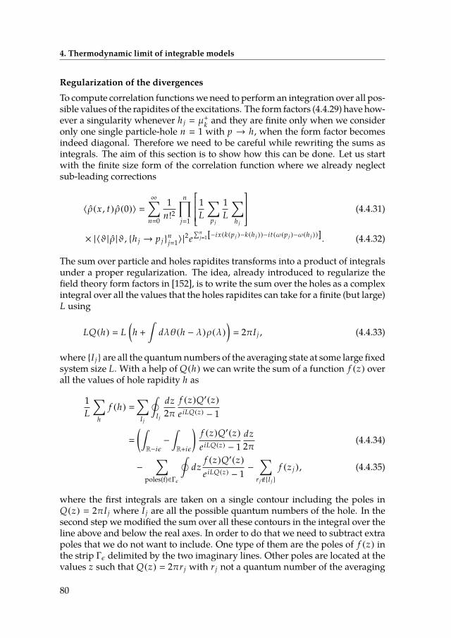
4. Thermodynamic limit of integrable models
Regularization of the divergencesTo compute correlation functionswe need to perform an integration over all pos-sible values of the rapidites of the excitations. The form factors (4.4.29) have how-ever a singularity whenever h j µ+
k and they are nite only when we consideronly one single particle-hole n 1 with p → h, when the form factor becomesindeed diagonal. Therefore we need to be careful while rewriting the sums asintegrals. The aim of this section is to show how this can be done. Let us startwith the nite size form of the correlation function where we already neglectsub-leading corrections
〈ρ(x , t)ρ(0)〉 ∞∑
n0
1n!2
n∏j1
1L
∑p j
1L
∑h j
(4.4.31)
× |〈ϑ |ρ |ϑ, h j → p j nj1〉|
2e∑n
j1[−ix(k(p j )−k(h j ))−it(ω(p j )−ω(h j ))]. (4.4.32)
The sum over particle and holes rapidites transforms into a product of integralsunder a proper regularization. The idea, already introduced to regularize theeld theory form factors in [152], is to write the sum over the holes as a complexintegral over all the values that the holes rapidites can take for a nite (but large)L using
LQ(h) L(h +ˆ
dλθ(h − λ)ρ(λ)) 2πI j , (4.4.33)
where I j are all the quantumnumbers of the averaging state at some large xedsystem size L. With a help of Q(h) we can write the sum of a function f (z) overall the values of hole rapidity h as
1L
∑h
f (h) ∑
I j
˛I j
dz2π
f (z)Q′(z)e iLQ(z) − 1
(ˆR−iε−
ˆR+iε
)f (z)Q′(z)e iLQ(z) − 1
dz2π (4.4.34)
−
∑poles(f)∈Γε
˛dz
f (z)Q′(z)e iLQ(z) − 1
−
∑r j<I j
f (z j ), (4.4.35)
where the rst integrals are taken on a single contour including the poles inQ(z) 2πI j where I j are all the possible quantum numbers of the hole. In thesecond step we modied the sum over all these contours in the integral over theline above and below the real axes. In order to do that we need to subtract extrapoles that we do not want to include. One type of them are the poles of f (z) inthe strip Γε delimited by the two imaginary lines. Other poles are located at thevalues z such that Q(z) 2πr j with r j not a quantum number of the averaging
80

4.4. Thermodynamic form factors
state (where holes cannot be created). When L →∞ only the integral above thereal line survives the limit (since Q(z) is monotonic in z) leading to
1L
∑h
f (h) ˆR+iε
f (z)ρ(z)dz − πi∑
res(f)∈Γε
f (z)ρ(z). (4.4.36)
If now we impose that f (z) has only a double pole in z p we can then rewritethe sum in terms of the nite part of the integral over h
1L
∑h
f (h) limε→0+
ˆ∞
−∞
dh f (h + iε) − πireshp
f (h) ?∞
−∞
dh f (h). (4.4.37)
In order to compute the nite part is then useful to compute the limit µ+j → h j
of the form factors (4.4.29)
|〈ϑ |ρ |ϑ, h j → µ+j
nj1〉|
|〈ϑ |ρ |ϑ, h j → µ+j
n−1j1 〉|
F(hn )
ρt (hn )(pn − hn )+ O(pn − hn ). (4.4.38)
where the back-ow is now computed as the sum of the other back-ows for theresidual excitations
F(λ | (p j , h j )nj1
)
n−1∑j1
F(λ | p j , h j
). (4.4.39)
Fredholm determinantWe are left with the problem of computing the thermodynamic limit of the de-terminant
Θ detN (δ jk + U jk )
V+p − V−p
(4.4.40)
where the matrix U is given in (4.4.4) and λp is an arbitrary number. Analo-gously to what is done in [150] we can take the limit λp →∞ leading to
Θ ic2∆k
det *.,δ jk +
i(µ j − λ j )V+
j − V−j
∏m, j
µm − λ j
λm − λ j
(2c
(λ j − λk )2 + c2−
2c
)+/-(4.4.41)
It is useful to consider a vector
a j i(µ j − λ j )V+
j − V−j
∏m, j
µm − λ j
λm − λ j. (4.4.42)
With this notation the determinant in (4.4.40) is expressed as
detN
(δi j + Ai j
), (4.4.43)
81

4. Thermodynamic limit of integrable models
with the matrix A given by
A jk a j
(K(λ j − λk ) −
2c
). (4.4.44)
Depending on j the vector a j has a dierent scaling behavior with the systemsize
a j ∼
O(1/L), λ j < λ−j nj1
O(1), λ j ∈ λ−j nj1
. (4.4.45)
We can use this property to simplify the computation of the determinant. Wedenote by a j a vector a j in which we substitute µ j by µ−j . Correspondingly wedene amatrix A jk with a j as a prefactor instead of a j . Thus the matrix elementsof A jk are all of O(1/L). By B jk we denote the dierence of the two matrices:B jk A jk−A jk . Note that thematrix B jk has only n non-zero rows correspondingto the excited rapidites λ−j
nj1. Using standard proprieties of the determinant
and assuming the matrix δi j + Ai j is invertible we can recast the determinant in aproduct of the determinant of an N ×N matrix and the determinant of an n × none
detN
(δi j + Ai j + Bi j ) detN
(δi j + Ai j ) × detn
*,δi j +
N∑k1
Bik
(1 + A
)−1k j
+-, (4.4.46)
where the indices i , j in the second determinant run only over the n excited ra-pidities and 1 denotes here the identity matrix. We can now take the thermody-namic limit. The rst determinant becomes a Fredholm determinant Det(1 + A)with the kernel
A(λ, µ) a(λ)(K(λ − µ) −
2c
), (4.4.47)
where a(λ j ) is the thermodynamic limit of ρ(λ j )a j . Standard computations give[150]
a(λ) ϑ(λ)F(λ)
Γ[1 + ϑ(λ)F(λ)]Γ[1 − ϑ(λ)F(λ)]
n∏k1µ−k ,λ
µ+k − λ
µ−k − λexp
[−PVˆ
dµϑ(µ)F(µ)µ − λ
]
×
2Im *
,
n∏k1
µ+k − λ + ic
µ−k − λ + icexp
[−
ˆdµϑ(µ)F(µ)µ − λ + ic
]+-
−1
. (4.4.48)
where the product∏n
k1µ−k ,λ
runs over all the holes (particles) except the j−th one
when λ µ−j for any j 1, . . . , n. With PV´we denoted the principal value of
82
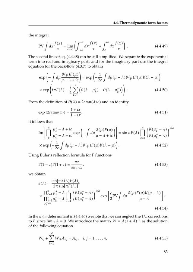
4.4. Thermodynamic form factors
the integral
PVˆ
dxf (x)
x limε→0
(ˆ−ε
−∞
dxf (x)
x+ˆ∞
εdx
f (x)x
). (4.4.49)
The second line of eq. (4.4.48) can be still simplied. We separate the exponentialterm into real and imaginary parts and for the imaginary part use the integralequation for the back-ow (4.3.7) to obtain
exp(−
ˆdµϑ(µ)F(µ)µ − λ + ic
) exp
(−
12c
ˆdµ(µ − λ)ϑ(µ)F(µ)K(λ − µ)
)× exp *
,iπF(λ) −
i2
n∑k1
(θ(λ − µ+
k ) − θ(λ − µ−k ))+
-. (4.4.50)
From the denition of θ(λ) 2atan(λ/c) and an identity
exp (2iatan(x)) 1 + ix1 − ix
, (4.4.51)
it follows that
Im
n∏k
µ+k − λ + ic
µ−k − λ + icexp
(−
ˆdµϑ(µ)F(µ)µ − λ + ic
) sin πF(λ)
n∏k1
(K(µ−k − λ)K(µ+
k − λ)
)1/2× exp
(−
12c
ˆdµ(µ − λ)ϑ(µ)F(µ)K(λ − µ)
). (4.4.52)
Using Euler’s reection formula for Γ functions
Γ(1 − z)Γ(1 + z) πz
sin πz, (4.4.53)
we obtain
a(λ) sin[πϑ(λ)F(λ)]2π sin[πF(λ)]
×
∏nk1 µ
+k − λ∏n
k1µ−k ,λ
µ−k − λ
n∏k1
( K(µ+k − λ)
K(µ−k − λ)
)1/2exp
[c2PVˆ
dµϑ(µ)F(µ)K(µ − λ)
µ − λ
].
(4.4.54)
In the n×n determinant in (4.4.46)wenote thatwe canneglect the 1/L correctionsto B since limth
nL 0. We introduce the matrix W A(1 + A)−1 as the solution
of the following equation
Wi j +N∑
k1WikAk j Ai j , i , j 1, . . . , n , (4.4.55)
83

4. Thermodynamic limit of integrable models
which in the thermodynamic limit becomes a linear integral equations for thefunction W (λ, µ)
W (λ, µ)+ˆ∞
−∞
dαW (λ, α) a(α)(K(α − µ) −
2c
) b(λ)
(K(λ − µ) −
2c
), (4.4.56)
with the vector b(λ) given by
b(λ) −sin[πϑ(λ)F(λ)]
2πϑ(λ)F(λ) sin[πF(λ)]
×
∏nk1 µ
+k − λ∏n
k1µ−k ,λ
µ−k − λ
n∏k1
( K(µ+k − λ)
K(µ−k − λ)
)1/2exp
[c2PV
ˆdµϑ(µ)F(µ)K(λ − µ)
λ − µ
].
(4.4.57)
Putting everything together we have then
limth detN
(δi j + Ai j + Bi j ) Det(1 + A) detn
(δi j + W (µ−i , µ
−
j )), (4.4.58)
and the determinant part of the form factors is then expressed as
Θ ic2∆k
Det(1 + A)detn(δi j + W (µ−i , µ
−
j )). (4.4.59)
Note that the Fredholm determinant is still a function of the excitations and notonly of the averaging state. This unfortunately poses still serious problems tothe computation of correlation functions. However from the numerical point ofview its evaluation can be eectively approximated with the very rst terms ofits expansion in powers of the trace.
Dynamical structure factor in 1/c expansion
We consider here the expansion in 1/c of the dynamical structure factor, denedas the Fourier transform of the density-density correlation
S(q , ω) ˆ
dxdt e iqx−iωt〈ϑ |ρ(x , t)ρ(0, 0) |ϑ〉
(2π)2∞∑
n0
1n!2
n∏j1
ˆ∞
−∞
dp jρh (p j )?∞
−∞
dh jρ(h j )δ *.
,q −
n∑j1
(k(p j ) − k(h j ))+/-
× δ *.,ω −
n∑j1
(ω(p j ) − ω(h j ))+/-|〈ϑ |ρ |ϑ, h j → p j
nj1〉|
2 ,
(4.4.60)
84

4.4. Thermodynamic form factors
for a generic thermal state at temperature T β−1 and density D 1. Expandingat the rst order in 1/c the only relevant form factors are the ones with only 1particle-hole excitation p , h µ+ , µ−
|〈ϑ |ρ |ϑ, h → p〉|
12π
1 + 2c
(ρt (h)ρt (p))1/2
[1 −
(p − h)2
πcPVˆ
dλϑ(λ)
(λ − p)(λ − h)
]+ O(1/c2),
(4.4.61)
since the ones with two or more particle-hole excitations contribute at the order1/c2 or higher. The lling fraction for a thermal state at temperature β, includingthe 1/c correction, is given by
ϑ(λ) 1 + 2
c
1 + eβ(λ2−h), (4.4.62)
with h the chemical potential xing the density D 1 of the gas. In the 1 particle-hole spectrum dynamical structure factor at S(q , ω) is given in terms of a singleform factor with energy ω andmomentum q times the density of states, which issimply the Jacobian of the transformation from the rapidities of the excitationsto the energy and momentum variable
p2− h2
ω, (4.4.63)
p − h q(1 + 2
c
)−1, (4.4.64)
which gives a Jacobian factor det∂(ω,q)∂(p ,h)
2q(1 + 2/c)−1 with the rapidities ofthe excitations given by
p q
2(1 + 2/c)+ ω(1 + 2/c)
2q, (4.4.65)
h −q
2(1 + 2/c)+ ω(1 + 2/c)
2q. (4.4.66)
We obtain then an expression for the thermal dynamical structure factor up to1/c2 corrections
S(q , ω) (2π)21 + 2
c
2q
[ρh (p)ρ(h) |〈ϑ |ρ |ϑ, h → p〉|
]
2π
*,π1 + 6
c
4q+ 12c
PVˆϑ(λ + p) − ϑ(λ + h)
λ+-ϑ(h)
(1 − ϑ(p)
)+ O(1/c2).
(4.4.67)
85
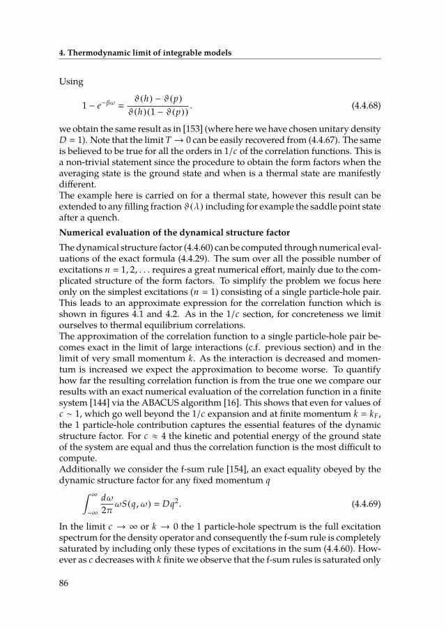
4. Thermodynamic limit of integrable models
Using
1 − e−βω ϑ(h) − ϑ(p)ϑ(h)(1 − ϑ(p))
. (4.4.68)
we obtain the same result as in [153] (where herewe have chosen unitary densityD 1). Note that the limit T → 0 can be easily recovered from (4.4.67). The sameis believed to be true for all the orders in 1/c of the correlation functions. This isa non-trivial statement since the procedure to obtain the form factors when theaveraging state is the ground state and when is a thermal state are manifestlydierent.The example here is carried on for a thermal state, however this result can beextended to any lling fraction ϑ(λ) including for example the saddle point stateafter a quench.Numerical evaluation of the dynamical structure factorThedynamical structure factor (4.4.60) can be computed throughnumerical eval-uations of the exact formula (4.4.29). The sum over all the possible number ofexcitations n 1, 2, . . . requires a great numerical eort, mainly due to the com-plicated structure of the form factors. To simplify the problem we focus hereonly on the simplest excitations (n 1) consisting of a single particle-hole pair.This leads to an approximate expression for the correlation function which isshown in gures 4.1 and 4.2. As in the 1/c section, for concreteness we limitourselves to thermal equilibrium correlations.The approximation of the correlation function to a single particle-hole pair be-comes exact in the limit of large interactions (c.f. previous section) and in thelimit of very small momentum k. As the interaction is decreased and momen-tum is increased we expect the approximation to become worse. To quantifyhow far the resulting correlation function is from the true one we compare ourresults with an exact numerical evaluation of the correlation function in a nitesystem [144] via the ABACUS algorithm [16]. This shows that even for values ofc ∼ 1, which go well beyond the 1/c expansion and at nite momentum k kF ,the 1 particle-hole contribution captures the essential features of the dynamicstructure factor. For c ≈ 4 the kinetic and potential energy of the ground stateof the system are equal and thus the correlation function is the most dicult tocompute.Additionally we consider the f-sum rule [154], an exact equality obeyed by thedynamic structure factor for any xed momentum q
ˆ∞
−∞
dω2π ωS(q , ω) Dq2. (4.4.69)
In the limit c → ∞ or k → 0 the 1 particle-hole spectrum is the full excitationspectrum for the density operator and consequently the f-sum rule is completelysaturated by including only these types of excitations in the sum (4.4.60). How-ever as c decreases with k nite we observe that the f-sum rules is saturated only
86
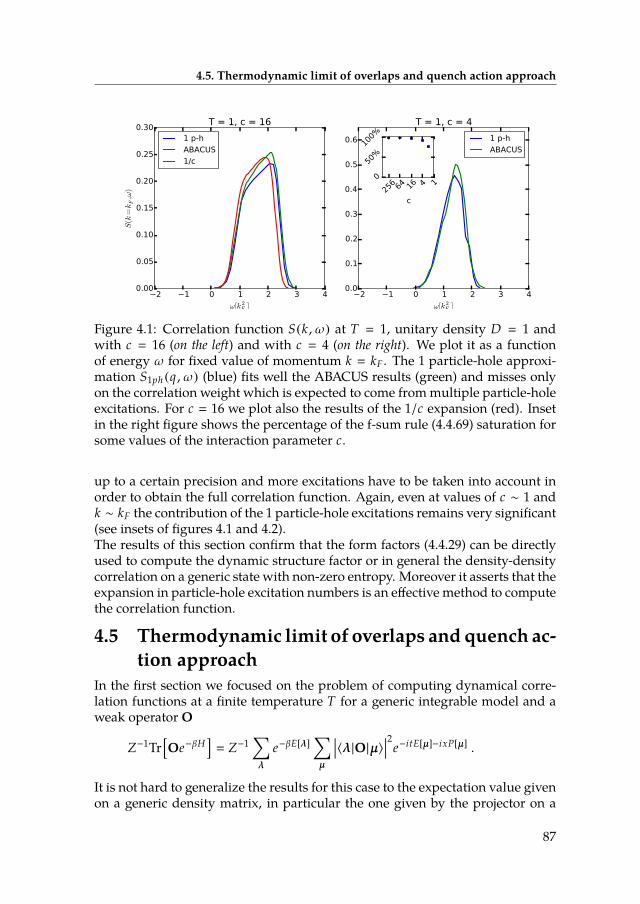
4.5. Thermodynamic limit of overlaps and quench action approach
2 1 0 1 2 3 4
ω[k 2F ]
0.00
0.05
0.10
0.15
0.20
0.25
0.30S(k
=kF,ω
)T = 1, c = 16
1 p-h
ABACUS
1/c
2 1 0 1 2 3 4
ω[k 2F ]
0.0
0.1
0.2
0.3
0.4
0.5
0.6
T = 1, c = 4
1 p-h
ABACUS
141664256
c
0
50%
100%
Figure 4.1: Correlation function S(k , ω) at T 1, unitary density D 1 andwith c 16 (on the left) and with c 4 (on the right). We plot it as a functionof energy ω for xed value of momentum k kF . The 1 particle-hole approxi-mation S1ph (q , ω) (blue) ts well the ABACUS results (green) and misses onlyon the correlation weight which is expected to come frommultiple particle-holeexcitations. For c 16 we plot also the results of the 1/c expansion (red). Insetin the right gure shows the percentage of the f-sum rule (4.4.69) saturation forsome values of the interaction parameter c.
up to a certain precision and more excitations have to be taken into account inorder to obtain the full correlation function. Again, even at values of c ∼ 1 andk ∼ kF the contribution of the 1 particle-hole excitations remains very signicant(see insets of gures 4.1 and 4.2).The results of this section conrm that the form factors (4.4.29) can be directlyused to compute the dynamic structure factor or in general the density-densitycorrelation on a generic state with non-zero entropy. Moreover it asserts that theexpansion in particle-hole excitation numbers is an eective method to computethe correlation function.
4.5 Thermodynamic limit of overlaps andquench ac-tion approach
In the rst section we focused on the problem of computing dynamical corre-lation functions at a nite temperature T for a generic integrable model and aweak operator O
Z−1Tr[Oe−βH
] Z−1
∑λ
e−βE[λ]∑µ
〈λ |O|µ〉2e−itE[µ]−ixP[µ] .
It is not hard to generalize the results for this case to the expectation value givenon a generic density matrix, in particular the one given by the projector on a
87
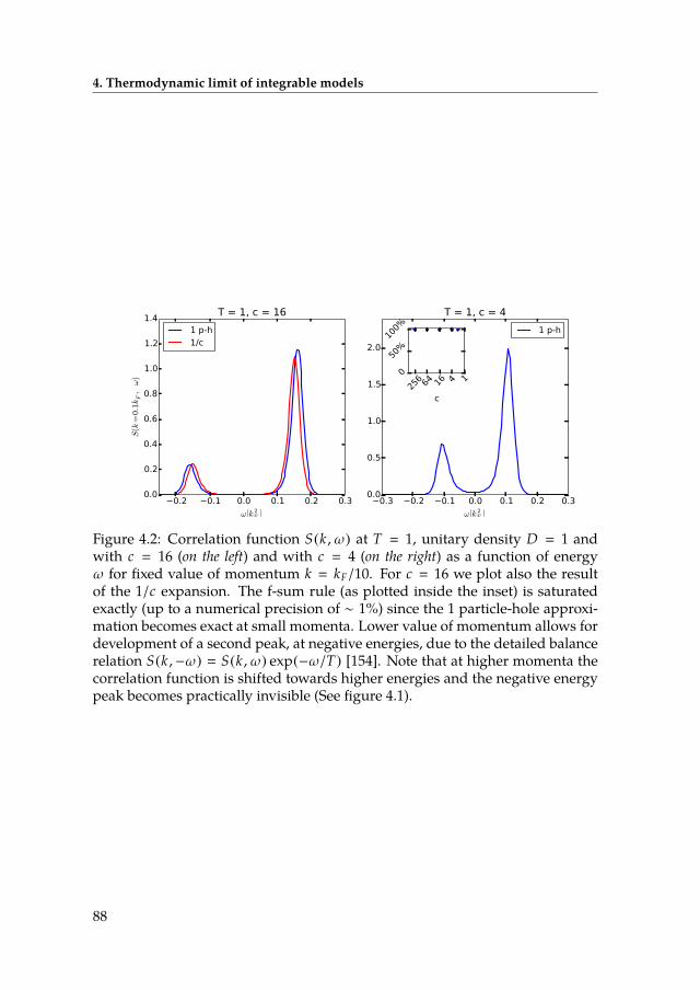
4. Thermodynamic limit of integrable models
0.2 0.1 0.0 0.1 0.2 0.3
ω[k 2F ]
0.0
0.2
0.4
0.6
0.8
1.0
1.2
1.4
S(k
=0.
1kF,ω)
T = 1, c = 16
1 p-h
1/c
0.3 0.2 0.1 0.0 0.1 0.2 0.3
ω[k 2F ]
0.0
0.5
1.0
1.5
2.0
T = 1, c = 4
1 p-h
141664256
c
0
50%
100%
Figure 4.2: Correlation function S(k , ω) at T 1, unitary density D 1 andwith c 16 (on the left) and with c 4 (on the right) as a function of energyω for xed value of momentum k kF/10. For c 16 we plot also the resultof the 1/c expansion. The f-sum rule (as plotted inside the inset) is saturatedexactly (up to a numerical precision of ∼ 1%) since the 1 particle-hole approxi-mation becomes exact at small momenta. Lower value of momentum allows fordevelopment of a second peak, at negative energies, due to the detailed balancerelation S(k ,−ω) S(k , ω) exp(−ω/T) [154]. Note that at higher momenta thecorrelation function is shifted towards higher energies and the negative energypeak becomes practically invisible (See gure 4.1).
88
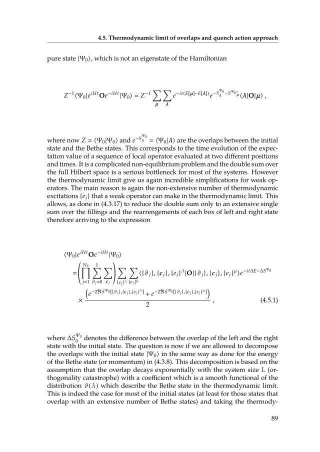
4.5. Thermodynamic limit of overlaps and quench action approach
pure state |Ψ0〉, which is not an eigenstate of the Hamiltonian
Z−1〈Ψ0 |e iHtOe−iHt|Ψ0〉 Z−1
∑µ
∑λ
e−it(E[µ]−E[λ]) e−SΨ0λ −SΨ0 ∗µ 〈λ |O|µ〉 ,
where now Z 〈Ψ0 |Ψ0〉 and e−SΨ0λ 〈Ψ0 |λ〉 are the overlaps between the initialstate and the Bethe states. This corresponds to the time evolution of the expec-tation value of a sequence of local operator evaluated at two dierent positionsand times. It is a complicated non-equilibriumproblem and the double sumoverthe full Hilbert space is a serious bottleneck for most of the systems. Howeverthe thermodynamic limit give us again incredible simplications for weak op-erators. The main reason is again the non-extensive number of thermodynamicexcitations e j that a weak operator can make in the thermodynamic limit. Thisallows, as done in (4.3.17) to reduce the double sum only to an extensive singlesum over the llings and the rearrengements of each box of left and right statetherefore arriving to the expression
〈Ψ0 |e iHtOe−iHt|Ψ0〉
*.,
Nb∏j1
1∑ϑ j0
∑c j
+/-
∑e j λ
∑e j
µ
〈ϑ j , c j , e j λ|O|ϑ j , c j , e j
µ〉e−it∆E−∆SΨ0
×
(e−2<SΨ0 [ϑ j ,c j ,e j
λ] + e−2<SΨ0 [ϑ j ,c j ,e j µ])
2 , (4.5.1)
where ∆SΨ00 denotes the dierence between the overlap of the left and the right
state with the initial state. The question is now if we are allowed to decomposethe overlaps with the initial state |Ψ0〉 in the same way as done for the energyof the Bethe state (or momentum) in (4.3.8). This decomposition is based on theassumption that the overlap decays exponentially with the system size L (or-thogonality catastrophe) with a coecient which is a smooth functional of thedistribution ϑ(λ) which describe the Bethe state in the thermodynamic limit.This is indeed the case for most of the initial states (at least for those states thatoverlap with an extensive number of Bethe states) and taking the thermody-
89

4. Thermodynamic limit of integrable models
namic limit of their overlap we obtain
SΨ0 [ϑλj , cλj , e j
λ] S[ϑ] + δs[ϑ, e j λ] + δs[ϑ, cλ] (4.5.2)
S[ϑ] Lˆ∞
−∞
dλ sΨ00 (λ)ρ(λ) (4.5.3)
δs[ϑ, c] ˆ∞
−∞
sΨ00 (λ)ϑ(λ)c(λ) (4.5.4)
δs[ϑ, e j ] m∑
k1
[sΨ00 (p j ) − sΨ0
0 (hk ) −ˆ∞
−∞
dλ sΨ00 (λ)ϑ(λ)F(λ |pk , hk )
],
(4.5.5)
where the function sΨ00 (λ) is a generalized single-particle overlap coecient and
e−S[ϑ] is the quench action generalization of the Gibbs factor e−βH . This is ob-tained by taking the extensive part of the overlap coecient Therefore we canproceed analogously to what is done in the thermal case obtaining
limth
Z−1〈Ψ0 |e iHtOe−iHt|Ψ0〉
12 lim
th
∑e j
〈ϑsp |O|ϑsp , e j 〉e−itω[ϑsp ,e j ]−δs[ϑsp ,e j ] +mirr. , (4.5.6)
where now the distribution ϑsp is still obtained as the saddle point of the gener-alized Free energy, namely the quench action
SQ[ϑ] 2<S[ϑ] − SYY[ϑ] , (4.5.7)
and it satises an integral equation simlar to the one for the thermal equilibrium(4.2.3)
εsp (λ) s0(λ) − h −12π
ˆ +∞
−∞
dµ K(λ − µ) log(1 + e−εsp (µ)
)(4.5.8)
ϑsp (λ) 1
1 + eε(λ) , (4.5.9)
where h is again a Lagrangemultiplier in charge of keeping the density constant(although it is not usually related to the chemical potential in (4.2.3))
ˆ∞
−∞
dλ ρsp (λ) n . (4.5.10)
The mirrored sum in (4.5.14) is simply the same sum where the exictations aredone on the left states instead than on the right one, namely
mirr. 12 lim
th
∑e j
〈ϑsp , e j |O|ϑsp〉e itω[ϑsp ,e j ]−δs∗[ϑsp ,e j ] , (4.5.11)
90
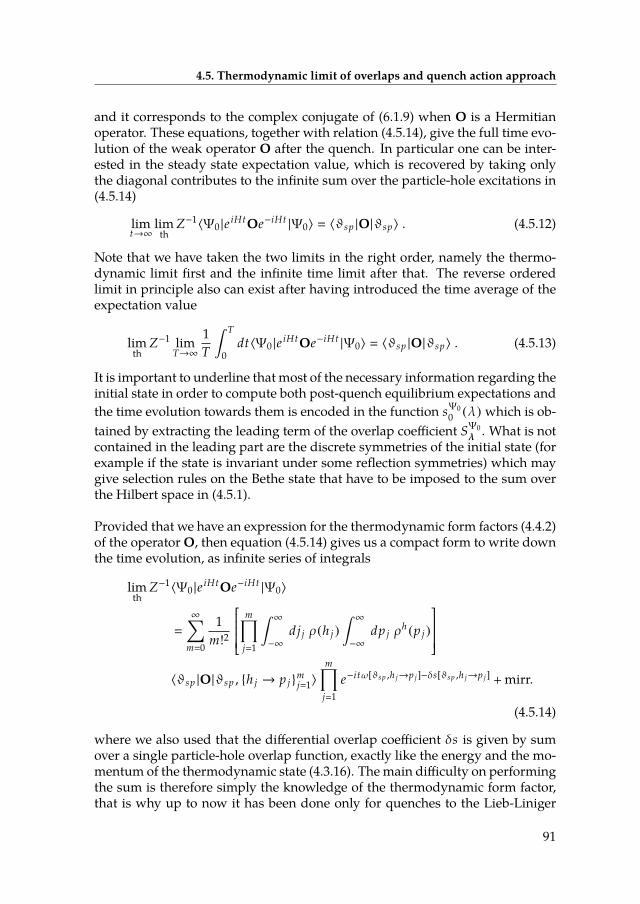
4.5. Thermodynamic limit of overlaps and quench action approach
and it corresponds to the complex conjugate of (6.1.9) when O is a Hermitianoperator. These equations, together with relation (4.5.14), give the full time evo-lution of the weak operator O after the quench. In particular one can be inter-ested in the steady state expectation value, which is recovered by taking onlythe diagonal contributes to the innite sum over the particle-hole excitations in(4.5.14)
limt→∞
limth
Z−1〈Ψ0 |e iHtOe−iHt|Ψ0〉 〈ϑsp |O|ϑsp〉 . (4.5.12)
Note that we have taken the two limits in the right order, namely the thermo-dynamic limit rst and the innite time limit after that. The reverse orderedlimit in principle also can exist after having introduced the time average of theexpectation value
limth
Z−1 limT→∞
1T
ˆ T
0dt〈Ψ0 |e iHtOe−iHt
|Ψ0〉 〈ϑsp |O|ϑsp〉 . (4.5.13)
It is important to underline that most of the necessary information regarding theinitial state in order to compute both post-quench equilibrium expectations andthe time evolution towards them is encoded in the function sΨ0
0 (λ) which is ob-tained by extracting the leading term of the overlap coecient SΨ0
λ . What is notcontained in the leading part are the discrete symmetries of the initial state (forexample if the state is invariant under some reection symmetries) which maygive selection rules on the Bethe state that have to be imposed to the sum overthe Hilbert space in (4.5.1).
Provided that we have an expression for the thermodynamic form factors (4.4.2)of the operatorO, then equation (4.5.14) gives us a compact form to write downthe time evolution, as innite series of integrals
limth
Z−1〈Ψ0 |e iHtOe−iHt|Ψ0〉
∞∑m0
1m!2
m∏j1
ˆ∞
−∞
dj j ρ(h j )ˆ∞
−∞
dp j ρh (p j )
〈ϑsp |O|ϑsp , h j → p j mj1〉
m∏j1
e−itω[ϑsp ,h j→p j ]−δs[ϑsp ,h j→p j ] +mirr.
(4.5.14)
where we also used that the dierential overlap coecient δs is given by sumover a single particle-hole overlap function, exactly like the energy and the mo-mentum of the thermodynamic state (4.3.16). Themain diculty on performingthe sum is therefore simply the knowledge of the thermodynamic form factor,that is why up to now it has been done only for quenches to the Lieb-Liniger
91

4. Thermodynamic limit of integrable models
model with large interaction parameter c → ∞. Otherwise the sum can beclearly computed numerically at nite, large system size using some discretiza-tions of the saddle point state (a set of representative states of the distributionϑsp) and performing the sum with the ABACUS algorithm [16] (See Chapter 6).
4.5.1 Single-particle overlap coecients: a conjectureEquation (4.5.2) shows that all the relevant information both for the saddle pointdistribution and for the whole time evolution is encoded in the function sΨ0
0 (λ)whichwedenoted as generalized single-particle overlap coecient. It is interest-ing to notice that for integrable models all the thermodynamic extensive quanti-ties (energy, momentum, rst conserved charges) are sums of the single-particleeigenvalues
E[λ] N∑
j1ε0(λ j ) . (4.5.15)
In order to compute the energy of a generic Bethe state therefore all what weneed to know is the single particle energy ε0(λ) and to solve the Bethe equationsfor the set λ. In the thermodynamic limit the latter is encoded in the distributionρ which therefore gives all the information necessary for the energy of the state
E[λ] Lˆ
dλ ρ(λ)ε0(λ) + ω[ρ, ex] , (4.5.16)
where ω[ρ, ex] is also a functional of the distribution ρ. We could argue thatthe same is valid also for the overlap-coecient, at least for some large class ofinitial states, like the translationally invariant initial states. Therefore we mayconjecture that the overlap of a generic Bethe state with such an initial state isgiven by
〈Ψ0 |λ〉 N∏
j1s0(λ j ) × R[λ] (4.5.17)
where R[λ] is a non extensive function, which therefore does not depend on thedetail of the state, such that
limth
R[λ]R[µ] 1 (4.5.18)
for states |λ〉, |µ〉 which dier for a non-extensive number of particle-hole exci-tations. Clearly one has to take into account that an overlap is also sensible todiscrete symmetries, (like parity invariance, see section 3.1) which may reducethe number of independent rapidites in the Bethe state. For the case of the BECinitial state in the Lieb-Liniger model and the Neél initial state for the XXZ spin
92
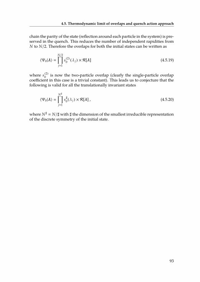
4.5. Thermodynamic limit of overlaps and quench action approach
chain the parity of the state (reection around each particle in the system) is pre-served in the quench. This reduces the number of independent rapidities fromN to N/2. Therefore the overlaps for both the initial states can be written as
〈Ψ0 |λ〉 N/2∏j1
s (2)0 (λ j ) × R[λ] (4.5.19)
where s (2)0 is now the two-particle overlap (clearly the single-particle overlap
coecient in this case is a trivial constant). This leads us to conjecture that thefollowing is valid for all the translationally invariant states
〈Ψ0 |λ〉 N ]∏j1
s]0 (λ j ) × R[λ] , (4.5.20)
where N ] N/]with ] the dimension of the smallest irreducible representationof the discrete symmetry of the initial state.
93

CHAPTER 5
The BEC quench in the Lieb-Linigermodel
Amid the pressure of great events, ageneral principle gives no help.
The Philosophy of History,G. W. F. Hegel
We consider a gas of δ−interacting bosons in the gound state of the theory inthe limit of zero interactions. This corresponds to the ground state of the many-body free bosonic theory, namely a Bose Einstein condensate (BEC) with a atwave function
〈x |BEC〉 ψBEC (x) L−N/2 (5.0.1)
where N is the total number of particles. At time t 0 we suddenly switch oninteractions and we let the state |BEC〉 evolve under the Lieb-Liniger Hamilto-nian. This corresponds to switch the coupling constant of the Lieb-Liniger gasfrom c0 0 to a nite c, what is usually denoted as an interaction quench.The rst question that one may ask is if the steady state expectation value of alocal observable O relaxes to an equilibrium value and how to compute it. Ifthe system relaxes canonically we can expect that a Gibbs ensemble reproducesthe late time expectation value of the operator Tr(e−βH O) where the eectivetemperature T 1/β is xed by the expectation value of the post-quench Hamil-tonian on the initial state 〈BEC |H |BEC〉 Tr(e−βH H). On the other hand weknow that the system has more local conserved quantities than just the Hamil-tonian which are then expected to inuence the relaxation of local observables.Moreover the energy uctuations of the initial state are divergent in the limit ofthe ultra-violet cut-o of the model Λ sent to innity
〈BEC |H2|BEC〉
∑λ
|〈λ |BEC〉|2 *.,
N∑j1λ2
j+/-
2
∼
ˆ Λ0
dλ →∞ (5.0.2)
which is another warning sign that we cannot expect to describe the relaxationof the system with a canonical Gibbs ensemble (see discussion on the eigenstatethermalization hypothesis in 1.2). In fact not even a Generalized Gibbs ensem-ble for this quench can be implemented due to the divergences of the conserved
95

5. The BEC quench in the Lieb-Liniger model
quantities on the initial state (which are present in any interaction quench insidethe Lieb-Liniger model). The successful approach turns out to be the quench ac-tionmethod, based on the exact expression of the overlaps (see section 3.1). Withthis approach we are then able to determine a macro-state |ρsp〉 (or equivalentlya thermodynamic Bethe state, introduced in chapter 4) which constitutes an ef-fective steady state for all the late time expectation values of local operators
limt→∞〈BEC(t) |O |BEC(t)〉 〈O〉eq ≡ 〈ρsp |O |ρsp〉 . (5.0.3)
We rst explain the origin of the divergences of the conserved charges on theinitial state (section 5.1), then we move to the thermodynamic limit of the over-laps (section 5.2), necessary to nd an exact expression for the steady state afterthe quench (section 5.3). This leads to predictions for the late time expectationvalues of local observables that can be also compared with the ones given by aneective thermal ensemble (section 5.4).
This chapter is based on the results published in [1].
5.1 The problem with the GGELet us imagine that we do not have the knowledge of the overlaps between theinitial state and the Bethe states. Therefore we are forced to use some other ap-proach. The rst one is to assume that the system for long time after the quenchis characterized by a density matrix and that this is given by the GGE assump-tion (see section 1.3). According to this, given a local observable O, the innitetime limit of its expectation value for long times after the quench is given by
limt→∞
limth
〈Ψ0 |O |Ψ0〉
〈Ψ0 |Ψ0〉
Tr[e−
∑n βn Qn O
]
Tr[e−
∑n βn Qn
] (5.1.1)
where the set of charges Qn are the local (extensive) conserved charges of thesystem. For the Lieb-Linigermodel there is a set of N of them,whose eigenvaluesare given by
Qn |λ〉 N∑
j1λn
j |λ〉 n 1, . . .N . (5.1.2)
In order to x their relative chemical potentials βn one has to compute theirexpectation values on the BEC state which is not an eigenstate. The chemicalpotentials are then xed by the condition
〈BEC |Qn |BEC〉 Tr
[e−
∑n βn Qn Qn
]
Tr[e−
∑n βn Qn
] , n 1, . . .N (5.1.3)
96
5.2. The problem with the GGE
In order to compute 〈BEC |Qn |BEC〉 we need an expression for the charges inreal space x. These are given in [155] which shows that the charges all have asimilar pattern
Qn ∼
N∑j1
∂n
∂xnj+α(1)
n cN∑
j1
(∂∂x j
)n−2 ∑1≥i> j≥N
δ(xi − x j )
+ . . . + α(n) *.,
c∑
1≥i> j≥N
δ(xi − x j )+/-
n/2
(5.1.4)
where c is the coupling constant of the Hamiltonian H ∼ Q2. The Bethe wavefunctions 2.2.13 have cusps whenever the position of two particles coincide xi
x j for any i , j 1, . . . ,N such that
limε→0+
∂xiΨ(x |λ)x j−ε− ∂xiΨ(x |λ)x j+ε
2c . (5.1.5)
Therefore when evaluated on a Bethe state the powers of δ−functions from thecharges (5.1.4) get canceled between each other and we obtain the regular ex-pression given in (5.1.2). However when applied to a Bethe state with dierentcoupling constant c′ the same cancellations do not happen and the expectationvalue of the charges become proportional to powers of ∼ (c − c′)δ(0) which cor-responds to an ultra-violet (UV) divergence ∼ 1/a where a is the lattice spacingof the model. The only way to regularize the expressions is to choose a latticeregularization, as for example the q−bosons model [156], nd the correspon-dent GGE density matrix and then take the limit a → 0. However this becomesa much harder problem to solve. Moreover it shows that in order to have a -nite GGE density matrix the innities present in the expectation values of thecharges have to cancel between each other in the nal sum
∑n βnQn in (5.1.1)
which makes therefore impossible to truncate the GGE to a limited amount ofconserved operators. In order to have a proper GGE ensemble one has to in-clude all the extensive charges Qn
Nn1 as proposed in [157]. However this is a
very complicated problem that up to now is not solved yet. On the other handit turned out that it is possible to compute the exact overlaps between the BECstate and the Lieb-Liniger Bethe states and to use the quench action formalismintroduced in section 4.5.
97
5. The BEC quench in the Lieb-Liniger model
5.2 Thermodynamic limit of the overlapsLet us consider the expression for the overlaps at nite size introduced in (3.1.27)
〈λ j ,−λ j N/2j1 |0〉
√√√√√√ (det N/2
j,k1GQjk
)2detNj,k1 G jk
√(cL)−N N!
N/2∏j1
λ jc
√λ2
j
c2 + 14
. (5.2.1)
In order to apply the quench action formalism we need to compute the thermo-dynamic limit of the above formula. Therefore we follow the same approach asin Chapter 4 to describe a generic thermodynamic Bethe state. We choose a seth j
mj1 (holes) of rapidities in the state and we change their values to a new set
p j mj1 (particles). Therfore in each box [λ, λ + dλ] there are Lρ(λ)dλ + np (λ) −
nh (λ) rapidites where np ,h is the number of particle or holes with rapidity λ.Moreover we introduce the displacements c(λ) which describes particle-holesshuings inside each box. With this notation we can take the thermodynamiclimit of the product in (5.2.1) analogously to how it is done for the energy of thestate (4.3.8)
limth logN/2∏j1
λ j
c
√λ2
j
c2+ 14
N/2∑j1
sBEC0 (λ j ) S[ϑ] + δs[ϑ, h j , p j mj1] + δs[ϑ, c] (5.2.2)
S[ϑ] Lˆ∞
0dλ sBEC0 (λ)ρ(λ) (5.2.3)
δs[ϑ, c] ˆ∞
0
∂sBEC0 (λ)∂λ
ϑ(λ)c(λ) (5.2.4)
δs[ϑ, h j , p j mj1]
m∑k1
[sBEC0 (pk ) − sBEC0 (hk )
−
ˆ∞
0dλ
∂sBEC0 (λ)∂λ
ϑ(λ)F(λ |pk , hk )], (5.2.5)
where the generalized single-particle overlap coecient (see also in 4.5.2) is givenby
sBEC0 (λ) log λc
√λ2
c2+ 14 . (5.2.6)
98
5.2. Thermodynamic limit of the overlaps
Note that since all the nite size states involved in the resolution of the BECstate are parity invariant states, the only particle-hole to consider are also parityinvariant excitations, namely
h j , p j mj1 h j ,−h j , p j ,−p j
m/2j1 . (5.2.7)
We now focus on the two determinants in Eq. (5.2.1).
R[λ,−λ]
(det N/2
j,k1GQjk
)2detNj,k1 G jk
. (5.2.8)
We can rewrite the determinant of the Gaudin matrix G jk as
detNj,k1 G jk LNN∏
j1
(1 + 1
L
N∑l1
K(λ j − λl ))
× detNj,k1 *,δ jk −
K(λ j − λk )
L +∑N
l1 K(λk − λl )+-. (5.2.9)
From the Bethe equations in the thermodynamic limit, Equation (4.1.10), wehave
1 + 1L
N∑l1
K(λ j − λl ) 2π ρt (λ j ) + O(1/L) , (5.2.10)
where ρt ρ + ρh . Furthermore, in the thermodynamic limit the matrix on theright-hand side of Eq. (5.2.9) becomes an integral operator on the real line:
δ jk −K(λ j − λk )
L +∑N
l1 K(λk − λl )→ 1 −
Kρ
2π ,
where(Kρ g
)(λ)
ˆ∞
−∞
dµ K(λ − µ)ρ(µ)ρt (µ)
g(µ) . (5.2.11)
The matrix GQjk can be analyzed analogously, using instead of Kρ the operator
KQρ acting as(
Kρ g)
(λ) Θ(λ)
×
ˆ∞
0dµ
[K(λ − µ) + K(λ + µ)
] ρ(µ)ρt (µ)
g(µ) , (5.2.12)
99
5. The BEC quench in the Lieb-Liniger model
where Θ(λ) is the Heaviside step function. Putting everything together, onends that in the thermodynamic limit the ratio of determinants in Eq. (5.2.1)becomes the ratio of two Fredholm determinants [158]
limth*..,
detN/2j,k1 GQjk√
detNj,k1 G jk
+//-
Det(1 − KQ
ρ
2π )√Det(1 − Kρ
2π )+ O(1/L) . (5.2.13)
Therefore the ratio of the two determinants (5.2.8) in the overlaps does not inu-ence the steady state and not even the time evolution towards it. Indeed since theratio of two Fredholmdeterminants is a non-extensive number, it is not extensiveand therefore does not inuence the saddle point state ϑsp and it is independentof the details of the state (namely the particle-hole excitation), therefore
limthR[λ,−λ]R[µ,−µ] 1 (5.2.14)
for Bethe states |λ,−λ〉, |µ,−µ〉 which dier up to a non-extensive number ofparticle-hole excitations.Finally, up to 1/L corrections and parts which are inessential to compute thepost-quench time evolution, the thermodydamic limit of the overlaps 5.2.1 isgiven only by the thermodynamic limit of the product (5.2.2)
limth
log〈λ,−λ |BEC〉 S[ϑ] + δs[ϑ, λ+j , λ
−
j mj1] + δs[ϑ, c] + . . . (5.2.15)
5.3 Explicit solution of the saddle point equationThe quench action now reads
SQ[ρ]/L
ˆ∞
0dλ
[ρ(λ) log
(λ2
c2
(14 + λ
2
c2
))− ρt (λ) log ρt (λ) + ρ(λ) log ρ(λ) + ρh (λ) log ρh (λ)
]. (5.3.1)
Note that we used a Yang-Yang entropy (4.1.15) with non-zero measure onlyon the half space λ > 0 since the lling of quantum numbers associated withthe negative rapidities is unambiguously determined by the positive ones andthus do not contribute to the entropy of the state. To impose the normalizationcondition on ρ we add a Lagrange multiplier h as in Ref. [106] which can beviewed, in the spirit of the free energy, as a generalized chemical potential. Thiscorresponds to modifying our functional measure as
ˆD[ρ] e−SQ [ρ]
→
ˆ +i∞
−i∞dhˆD[ρ] e−SQ [ρ]e−
Lh2 (n−
´∞
−∞dλρ(λ)) . (5.3.2)
100
5.3. Explicit solution of the saddle point equation
Taking the functional derivativewith respect to ρ andusingdimensionless quan-tities x λ/c and K(x) 2
x2+1 , we obtain as a saddle point equation a non-linearintegral equation for the function a(x) ≡ ρ(λ)/ρh (λ),
log a(x) log (τ2) − log[x2
(x2 + 1/4
)]
+ˆ∞
−∞
K(x − y) log[1 + a(y)
] dy2π , (5.3.3)
where τ is related to the Lagrange multiplier h via τ eh/2. The functions aand ρ are directly connected. Taking the derivative τ
2 ∂τ of Eq. (5.3.3) and due tothe thermodynamic form of the Bethe equations the function 2πρ(x) is given byτ2 ∂τa(x)/(1 + a(x)).The non-linear integral equation (5.3.3) has an analytical solution, which canbe derived as follows. In the limit τ → 0 the driving term becomes large andnegative for all xed x > τ and the convolution integral gives only subleadingcontributions. Thus, the rst non-trivial order of the function a(x) reads
a (0) (x) τ2
x2(x2 + 1/4). (5.3.4)
In order to calculate the next leading term, we plug this result into the convolu-tion integral on the right hand side of the saddle point equation (5.3.3). Usingthe relationˆ
∞
−∞
1/π(x − y)2 + 1
log[y2 + α2
]dy log
[x2 + (α + 1)2
], (5.3.5)
we obtain up to order τ2
log a(x) log (τ2)
− log[x2
(x2 + 1/4
) (x2 + 1
) (x2 + 9/4
)]
+ˆ∞
−∞
K(x − y) log[y2(y2 + 1/4) + τ2
] dy2π . (5.3.6)
By rewriting y2(y2+1/4)+τ2 (y2+ y2−)(y2+ y2
+) where y± 1√8
√1 ±√
1 − 64τ2,using Eq. (5.3.5) again and expanding y± to lowest order in τ: y+ 1/2 andy− 2τ, we get
a(x) τ2
(x2 + (1 + y−)2
) (x2 + (1 + y+)2
)x2(x2 + 1/4)(x2 + 1)(x2 + 9/4)
τ2
x2(x2 + 1/4)
[1 + 4τ(1 + τ)
x2 + 1
]. (5.3.7)
101

5. The BEC quench in the Lieb-Liniger model
Hence, the function a(x)/a (0) (x) up to rst order in τ reads
a (1) (x)a (0) (x)
1 + 4τx2 + 1
. (5.3.8)
Repeating this procedure we can calculate higher orders in τ systematically,leading to an expression up to generic order τN
a (N) (x)a (0) (x)
N+1∑n1
(2n
n − 1
) n∏j2
τ
x2 + ( j/2)2. (5.3.9)
The limit N →∞ leads to the solution of the saddle point equation (5.3.3),
a(x) limN→∞
a (N) (x) ∞∑
n1
(2n
n − 1
) n∏j0
τ
x2 + ( j/2)2
2πτ
x sinh (2πx)I1−2ix
(4√τ)I1+2ix
(4√τ). (5.3.10)
Here, In (z) is the modied Bessel function of the rst kind of order n. We even-tually get
2πρ(x) τ2 ∂τa(x)1 + a(x)
a(x)
1 + a(x)τ∂τ2 log a(x) . (5.3.11)
Note that the saddle point distribution ρsp is then given by ρsp(λ) ρ(λ/c).The computation of the dimensionless particle density N/(Lc) n/c 1/γ andenergy density E/(Lc3) e/c3 by numerical integration of function (6.2.4) yields
nc
ˆ∞
−∞
ρ(x)dx τ ,ec3
ˆ∞
−∞
x2ρ(x)dx τ2 , (5.3.12)
i.e. τ 1/γ and e cn2 γn3, in agreement with the initial energy density
limth L−1〈BEC |HLL |BEC〉 γn3 . (5.3.13)
5.4 Physical properties of the steady stateThe saddle point distribution gives us access, in principle, to any correlationfunction of operators allowed within the quench action approach. We focus ondensity correlations. Following the method of [159, 160] we compute in Fig. 5.2the static density moments g2 and g3 dened by
gK 〈ρsp | : (ρ(0)/n)K: |ρsp〉 . (5.4.1)
102
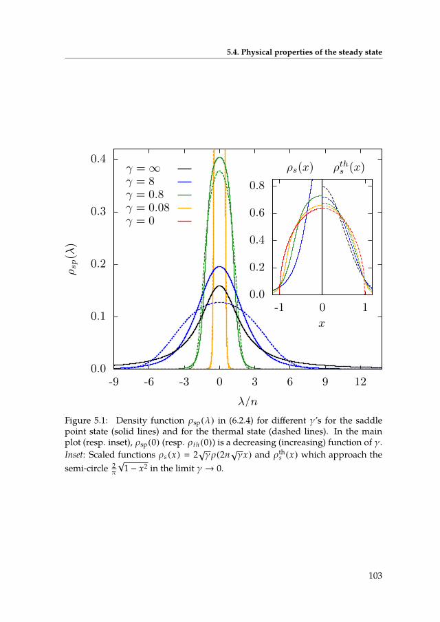
5.4. Physical properties of the steady state
0.0
0.1
0.2
0.3
0.4
-9 -6 -3 0 3 6 9 12
λ/n
ρsp(λ)
0.0
0.2
0.4
0.6
0.8
-1 0 1
ρs(x) ρths (x)
x
γ = 0γ = 0.08γ = 0.8γ = 8γ = ∞
Figure 5.1: Density function ρsp(λ) in (6.2.4) for dierent γ’s for the saddlepoint state (solid lines) and for the thermal state (dashed lines). In the mainplot (resp. inset), ρsp(0) (resp. ρth (0)) is a decreasing (increasing) function of γ.Inset: Scaled functions ρs (x) 2√γρ(2n
√γx) and ρths (x) which approach the
semi-circle 2π
√
1 − x2 in the limit γ → 0.
103

5. The BEC quench in the Lieb-Liniger model
0.0
0.2
0.4
0.6
0.8
1.0
0 1 2 3 4 5 6 7 8
γ
g K(γ)
1−√γ
2
1− 3√γ
2
0.8
0.9
1.0
0.0 0.03γ 10−6
10−4
10−2
100
100 101 102 103
γ
g2
g3
gth2gth3
Figure 5.2: Expectation values g2 (red, upper curve) and g3 (green, lower curve)as function of γ on the exact saddle point state (solid lines) and on the thermalone (dashed lines). Asymptotic behaviours (black dashed lines) g2 ∼ 8/(3γ),g3 ∼ 32/(15γ2) for γ → ∞ as in [156] and g2 ∼ 1 − √γ/2, g3 ∼ 1 − 3√γ/2 forγ → 0. Insets: Same plot (in logarithmic scale) for dierent ranges of γ.
104

5.5. Asymptotics of the saddle point distribution
The density operator is dened as ρ(x) Ψ†(x)Ψ(x), where the operators ¯(x)satises the canonical commutation relations [Ψ(x),Ψ†(x′)] δ(x−x′). Resultsfor the saddle point state are compared with the ones obtained using a thermalstate at xed particle density n and energy density e n3γ. These results clearlydisplay the lack of thermalization long after the quench.In Fig. 5.3 we further address static correlations by studying the static structurefactor S(x) 〈Isp |ρ(x)ρ(0) |Isp〉 and its Fourier transform using the Lehmannrepresentation
S(k) L∑
I
|〈Isp |ρ(0) |I〉|2δk ,PI , (5.4.2)
where the state |Isp〉 scales to the saddle point distribution. The matrix elementsare known exactly through the method of Algebraic Bethe Ansatz [149] andsummed into correlations by the ABACUS algorithm [16] following the methodin Ref. [144].
5.5 Asymptotics of the saddle point distributionThe asymptotic expansion of the saddle point distribution 2πρ(x) in Eq. (6.2.4)for x →∞ and arbitrary xed 0 < τ < ∞ is given by (up to O
(x−10
))
2πρ(x) ∼τ2
x4 −τ2 − 24τ3
4x6 + τ2− 120τ3 + 464τ4
16x8 . (5.5.1)
The rst two terms were previously found within an approach using q-Bosons[156]. The Tonks-Girardeau limit c → ∞ at xed density n, i.e. τ → 0, can beeasily performed,
a(x) ∼ a (0) (x) τ2
x2(x2 + 1/4)
⇒ 2πρ(x) ∼τ2
x2(x2 + 1/4) + τ2. (5.5.2)
Substituting τ n/c and x λ/c yields 2πρsp(λ) ∼ 4n2/(λ2 + 4n2).The limit c → 0 at xed density n, i.e. τ → ∞, is more complicated. The rstobservation is that the scaled density ρs (x) 2ρ(2
√τx)/√τ, calculated by using
the exact expression (5.3.10), has a proper limit,
limτ→∞
ρs (x) limτ→∞
2ρ(2√τx)
√τ
2π
√
1 − x2 Θ(1 − x2)
⇒ ρ(x) ∼√τ
π
√1 − x2
4τ Θ(4τ − x2) . (5.5.3)
105
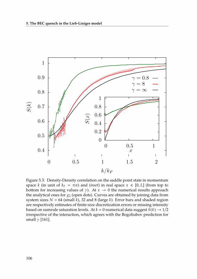
5. The BEC quench in the Lieb-Liniger model
0.4
0.5
0.6
0.7
0.8
0.9
1
0 0.5 1 1.5 2
k/kF
S(k)
0
0.2
0.4
0.6
0.8
1
0 0.5 1
S(x)
x
γ = 0.8γ = 8γ = ∞
Figure 5.3: Density-Density correlation on the saddle point state in momentumspace k (in unit of kF πn) and (inset) in real space x ∈ [0, L] (from top tobottom for increasing values of γ). At x → 0 the numerical results approachthe analytical ones for g2 (open dots). Curves are obtained by joining data fromsystem sizes N 64 (small k), 32 and 8 (large k). Error bars and shaded regionare respectively estimates of nite-size discretization errors or missing intensitybased on sumrule saturation levels. At k 0 numerical data suggest S(k) → 1/2irrespective of the interaction, which agrees with the Bogoliubov prediction forsmall γ [161].
106
5.5. Asymptotics of the saddle point distribution
This can be proven by analyzing the asymptotic behavior of Bessel functions.First of all we write
2π2ρ(2
√τx)
√τ
√τ∂τa(2
√τx , τ)
1 + a(2√τx , τ)
a(2√τx , τ)
1 + a(2√τx , τ)
√τ∂τa(2
√τx , τ)
a(2√τx , τ)
, (5.5.4)
where the partial derivative is with respect to the second argument. We analyzethe two factors separately. The rst one becomes
limτ→∞
a(2√τx , τ)
1 + a(2√τx , τ)
1 for |x | ≤ 1
f (x) for |x | > 1 , (5.5.5)
where f is a function with f (1) 1, and which decays algebraically as (2x)−4for large x. In order to analyze the second factor in Eq. (5.5.3) we set z 4
√τ.
Using formula (5.3.10) and the abbreviation ν xz we obtain, due to τ∂τ z2∂z
and I′ν (z) (Iν+1(z) + Iν−1(z))/2,√τ∂τa(2
√τx , τ)
a(2√τx , τ)
4z+ I−iν (z)
I1−iν (z)+ I2−iν (z)
I1−iν (z)+ Iiν (z)
I1+iν (z)+ I2+iν (z)
I1+iν (z)
4<[ I−iν (z)
I1−iν (z)
]. (5.5.6)
Note that the partial derivative acts only on the argument, but not on the order ofthe modied Bessel functions. Now we use the uniform asymptotic limit of themodied Bessel function of the rst kind, which is also known as the uniformAiry-type asymptotic expansion of Bessel functions [162]:
I−iν (νz′) ∼eπν/2
2ν1/3( 4ζ1 − z′2
)1/4
[Bi(−ν2/3ζ) + 2ie−πν sinh (πν)Ai(−ν2/3ζ)
] ∞∑s0
(−1)s As (ζ)ν2s
+[Bi′(−ν2/3ζ) + 2ie−πν sinh (πν)Ai′(−ν2/3ζ)
] ∞∑s0
(−1)s Bs (ζ)ν2s+4/3
, (5.5.7)
where 23ζ
3/2 log(1+√
1−z′2z′
)−
√
1 − z′2. Ai and Bi are Airy functions and thelowest expansion coecients are given by A0 B0 1. Expanding the quotientin Eq. (5.5.6) for large z to the leading asymptotic order we have to bear in mind
107
5. The BEC quench in the Lieb-Liniger model
that, in the denominator, imaginary order and argument are ν+ i and z′ν/(ν+ i),respectively, instead of ν and z′ 1/x as in the numerator. Using the asymptoticexpansions of Airy functions
Ai(−z) ∼sin
(23 z3/2 + π
4
)√πz1/4
, Bi(−z) ∼cos
(23 z3/2 + π
4
)√πz1/4
, (5.5.8)
we eventually obtain by putting z νz′ ν/x
<
[ I−ixz (z)I1−ixz (z)
]
z→∞<
[ I−iν (νz′)I1−iν (νz′)
]νxz→∞z′1/x<∞
∼ <
1 +√
1 − z′2
iz′
νxz→∞z′1/x<∞
Θ(1 − x2)√
1 − x2 . (5.5.9)
In the last step we used that, due to the real part, the leading order is only non-zero if the absolute value of x is less than one. For |x | > 1 the leading ordervanishes andwehave limτ→∞ ρs (x) 0 for every xed |x | > 1. Taking the factors2π and 4 in Eqs. (5.5.4) and (5.5.6) into account we nally get ρs (x) 2
π
√
1 − x2
for |x | ≤ 1 and ρs (x) 0 elsewhere, which proves Eq. (5.5.3).Substituting τ n/c 1/γ, x λ/c in Eq. (5.5.3) and dening λ∗ 2n
√γ, we
obtain
ρsp(λ) ∼ n2πλ∗
√1 − λ
2
λ2∗
Θ(λ∗ − |λ |) . (5.5.10)
which reproduces the leading term of the ground state distribution of the Lieb-Liniger model in the low-γ expansion.
108

CHAPTER 6
Post-quench time evolution ofintegrable models
I intend to live forever, or die trying.
G. Marx
Most of the theoretical research on the relaxation of isolated quantum systemsfollowing a quantum quench focused so far on the expectation values of localobservables at late times after the quench, when the system is in an eectivesteady state. For example the GGE hypothesis focuses on the possibility of re-ducing the huge complexity of the initial wave function to a reduced set of in-formation, incorporated in the local conserved quantities of the system, whichgives the expectation values of all physical observables in the steady state. How-ever the question of how to perform an analogous simplication for the wholepost-quench time evolution, has been poorly addressed, except in a few cases 1.In particular we would like to know if we can understand relaxation time scales,eective velocity of propagation of the excitations in the system and even thefull post-quench time evolution from a reduced set of macroscopic data on theinitial state. These predictions are clearly much more interesting than late timeexpectation values from the expermental point of view, since experiments areusually limited in the range of time (the typical life time of a cold atom experi-ments is roughly 10-100 µs). Moreover the late time dynamics is expected to beinuenced much more by the impurities in the system (the trap conning theatoms of the gas, a spin impurity in the chain are typical examples) than theshort time one.
The quench action method introduced in section 4.5 has proved to oer a pro-cedure whereby one can derive, from rst principles, not only the steady stateitself but also the actual time evolution of physical observables . In this chapterwe show that this approach is able to provide the full post-quench time evolu-tion in terms of a reduced set of data which can be extracted from the thermo-dynamically leading part of the overlaps. It turns out that the same function, thegeneralized single-particle overlap coecient sΨ0
0 (λ) (see section 4.5), xes thesteady-state expectation values and the whole time evolution from t 0+ afterthe quench. This is treated analogously to a system at thermal equilibrium with
1Some references on the topic are [34, 63, 64, 67, 68, 79–81,87, 90, 126, 163–170].
109

6. Post-quench time evolution of integrable models
a sub-entropic gas of independent particle-hole excitations around the steadystate constituting the whole eective spectrum necessary to compute the timedependence of all physical observables. A restricted class of excitations is thenclearly seen to be the most relevant for the long-time behavior, giving a picturereminiscent of a eld theory description of the asymptotics of correlations inequilibrium situations [171–173].
We rst review (section 6.1) how the method of the quench action provides theexact time evolution after a quench in a generic integrable model (in fact anymodel where we can write down its eigenstates) and how from this we obtainan expression for the power law decay towards equilibrium of local operatorsafter a generic quench [8]. Then we apply the method to compute the wholetime evolution of the static density function after a quench from the BEC stateto the Lieb-Liniger gas with nite coupling constant c (section 6.2). Then we ad-dress the time evolution of more complicated correlation functions in the limitof hard-core bosons, when the coupling constant is very large c → ∞ (section6.3).
This chapter is based on the results published in [1, 6, 8].
6.1 The quench action method and the post-quenchevolution in an integrable model
Weconsider an initial state |Ψ0〉which is not an eigenstate of the one-dimensionalintegrable Hamiltonian H for N particles moving on a system size L with peri-odic boundary conditions. In a generic integrable model each eigenstate is spec-ied by a set of N quantum numbers I I j
Nj1. The set of nonlinear coupled
Bethe equations maps the mutually excluding quantum numbers in N quasi-momenta, called rapidites, I → λ λ j
Nj1 which take value in the complex
plane. These are related to the one-particle momentum k0(λ) and the scatteringphase of the model θ(λ) [106]
k0(λi ) 2πIi
L−
1L
N∑k1
θ(λi − λk ) i 1, . . . ,N . (6.1.1)
All the possible dierent choices of quantum numbers I give a complete basisof eigenstates |λ〉 with energy E[λ] which allows, given a local operator O, toresolve the time evolution of its expectation value on the initial state
〈Ψ0 |e iHt Oe−iHt|Ψ0〉 ≡ 〈O(t)〉 , (6.1.2)
〈O(t)〉 ∑λ
∑µ
e−SΨ0λ e−(SΨ0 )∗µ 〈λ |O |µ〉e−it(E[µ]−E[λ]) , (6.1.3)
110
6.1. The quench action method and the post-quench evolution in an integrable model
where we introduced the overlap coecients SΨ0λ between the initial state and
the eigenstates 〈Ψ0 |λ〉 e−SΨ0λ . The double sum in (6.1.3) can be performed ingeneral when the number N of constituents of the system is small. Howeverone is in general interested in the thermodynamic limit limth ≡ limN,L→∞ withxed density n N/L. The quench action approach introduced in [79] allows tomove from a sum over the discrete representation for the eigenstates, in termsof the quantum numbers I to a functional integral over smooth distributionsof rapidites and simple excitations over them. Given a smooth function ρ(λ) ofrapidities on the real axis with its normalization given by the density of particles´∞
−∞dλ ρ(λ) n (under the string hypothesis it can be generalized to complex
rapidities [174]), there is an entropic number ∼ eSYY [ρ] of nite size states thatshare the same expectation values of local operators [106]. The entropy is givenby [118]
SYY[ρ] Lˆ∞
−∞
dλ((ρ + ρh ) ln(ρ + ρh ) − ρ ln ρ − ρh ln ρh) , (6.1.4)
where the density of holes is given by the total density ρh ρt−ρ, related to the
density of particles by the Bethe equations (6.1.1) in the thermodynamic limit
ρt
12π
(k0 + θ ∗ ρ
), (6.1.5)
where we introduce the convolution between two functions f ∗ g ´∞
−∞dµ f (λ−
µ)g(µ) and the derivative respect to λ, d fdλ ≡ f . For later convenience we also
introduce the scalar product on the real axis f · g ´∞
−∞dµ f (µ)g(µ). After
restricting to the appropriate sub-Hilbert space with nonzero overlap (if dis-crete symmetries are present), the overlaps become a smooth functional over theeigenstates. In particular they can be written as an extensive universal part (de-pendent only on the distribution ρ) with subleading corrections which dependon the nite number of particle-hole excitations hi , pi
mi1 over the distribution
ρ (which corresponds to displacing a number m of quantum numbers of one ofthe nite size state |λ〉 → |ρ〉 which discretizes the distribution ρ)
SΨ0λ → S[ρ] + δs[ρ, hi , pi
mi1] + O(1/N) , (6.1.6)
where both quantities are given in terms of the generalized one-particle overlapcoecient sΨ0
0 (λ)
S[ρ] L sΨ00 · ρ ,
δs[ρ, hi , pi mi1]
m∑k1
(sΨ00 (pk ) − sΨ0
0 (hk ) − Fk · sΨ00
). (6.1.7)
111
6. Post-quench time evolution of integrable models
The back-ow Fk (λ) for a single particle-hole is computed in terms of the distri-bution ρ
2πFkρt
ρθ(λ − pk ) − θ(λ − hk ) + θ ∗ Fk . (6.1.8)
Therefore in the thermodynamic limit, for any weak operator, we can write itstime-dependent expectation value (6.1.3) as
limth〈O(t)〉
12
ˆDρ e−2<S[ρ]+SYY [ρ]
∞∑m0
ˆd[h , p]m
[e−δs[ρ,hi ,pi
mi1]−itω[ρ,hi ,pi
mi1]〈ρ |O |ρ, hi , pi
mi1〉
]+mirr , (6.1.9)
with´
d[h , p]m 1
(m!)2∏m
j1´∞
−∞dh jρ(h j )
´∞
−∞dp jρh (p j ) denoting the sum over
themacroscopic particle-hole excitations andmirr indicating the same sum as in(6.1.9) but with excitations on the left state. The energy of a state E[λ]→ E[ρ] +ω[ρ, hi , pi
mi1] is given in terms of the one-particle energy ε0(λ) analogously to
the overlaps (6.1.7)
E[ρ] L ε0 · ρ ,
ω[ρ, hi , pi mi1]
m∑k1
(ε0(pk ) − ε0(hk ) − Fk · ε0
).
The matrix elements 〈ρ |O |ρ〉 can be computed by choosing one of the possi-ble (large) nite size realizations |λ〉 → |ρ〉 of the distribution ρ(λ) and us-ing 〈ρ |O |ρ〉
〈ρ |ρ〉 〈λ |O |λ〉〈λ |λ〉
(1 + O(1/N)
). The same can be done for the o diagonal
ones. Given these ingredients the sum in (6.1.3) can be evaluated in the saddlepoint δSQ [ρ]
δρρρsp
0 of the quench action SQ[ρ] 2<S[ρ] − SYY[ρ] leading toan expression for the whole post-quench time evolution in the thermodynamiclimit [1, 79]
limth〈O(t)〉
12
∞∑m0
ˆd[h , p]m
[e−it(ω[ρsp ,hi ,pi
mi1])
× e−δs[ρsp ,hi ,pi mi1]〈ρsp |O |ρsp , hi , pi
mi1〉
]+mirr. (6.1.10)
A notable consequence of formula (6.1.10) is that all the information to recon-struct the entire post-quench time evolution is contained in the function sΨ0
0 (λ)which can be extracted by taking the scaling limit of the overlap coecients
SΨ0λ
N∑j1
(sΨ00 (λ j ) + O(N−1)
). (6.1.11)
112
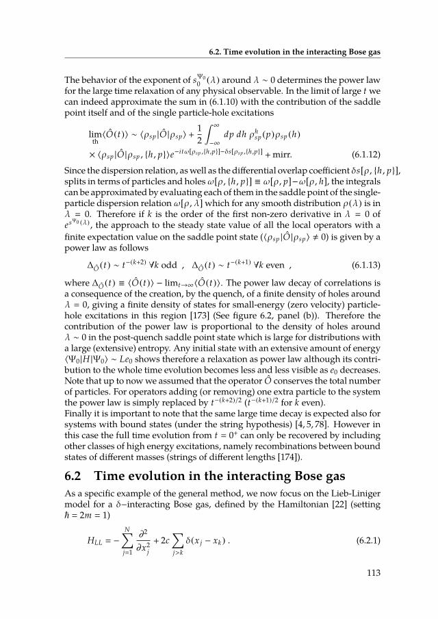
6.2. Time evolution in the interacting Bose gas
The behavior of the exponent of sΨ00 (λ) around λ ∼ 0 determines the power law
for the large time relaxation of any physical observable. In the limit of large t wecan indeed approximate the sum in (6.1.10) with the contribution of the saddlepoint itself and of the single particle-hole excitations
limth〈O(t)〉 ∼ 〈ρsp |O |ρsp〉 +
12
ˆ∞
−∞
dp dh ρhsp (p)ρsp (h)
× 〈ρsp |O |ρsp , h , p〉e−itω[ρsp ,h ,p]−δs[ρsp ,h ,p] +mirr. (6.1.12)
Since the dispersion relation, aswell as the dierential overlap coecient δs[ρ, h , p],splits in terms of particles and holes ω[ρ, h , p] ≡ ω[ρ, p]−ω[ρ, h], the integralscan be approximated by evaluating each of them in the saddle point of the single-particle dispersion relation ω[ρ, λ] which for any smooth distribution ρ(λ) is inλ 0. Therefore if k is the order of the rst non-zero derivative in λ 0 ofe sΨ0 (λ) , the approach to the steady state value of all the local operators with anite expectation value on the saddle point state (〈ρsp |O |ρsp〉 , 0) is given by apower law as follows
∆O (t) ∼ t−(k+2)∀k odd , ∆O (t) ∼ t−(k+1)
∀k even , (6.1.13)
where ∆O (t) ≡ 〈O(t)〉 − limt→∞〈O(t)〉. The power law decay of correlations isa consequence of the creation, by the quench, of a nite density of holes aroundλ 0, giving a nite density of states for small-energy (zero velocity) particle-hole excitations in this region [173] (See gure 6.2, panel (b)). Therefore thecontribution of the power law is proportional to the density of holes aroundλ ∼ 0 in the post-quench saddle point state which is large for distributions witha large (extensive) entropy. Any initial state with an extensive amount of energy〈Ψ0 |H |Ψ0〉 ∼ Le0 shows therefore a relaxation as power law although its contri-bution to the whole time evolution becomes less and less visible as e0 decreases.Note that up to nowwe assumed that the operator O conserves the total numberof particles. For operators adding (or removing) one extra particle to the systemthe power law is simply replaced by t−(k+2)/2 (t−(k+1)/2 for k even).Finally it is important to note that the same large time decay is expected also forsystems with bound states (under the string hypothesis) [4, 5, 78]. However inthis case the full time evolution from t 0+ can only be recovered by includingother classes of high energy excitations, namely recombinations between boundstates of dierent masses (strings of dierent lengths [174]).
6.2 Time evolution in the interacting Bose gasAs a specic example of the general method, we now focus on the Lieb-Linigermodel for a δ−interacting Bose gas, dened by the Hamiltonian [22] (setting~ 2m 1)
HLL −
N∑j1
∂2
∂x2j
+ 2c∑j>k
δ(x j − xk ) . (6.2.1)
113
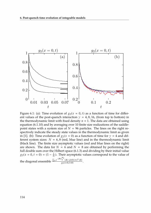
6. Post-quench time evolution of integrable models
0
0.2
0.4
0.6
0.8
1
0.01 0.03 0.05 0.07
(a)
0.2
0.4
0.6
0.8
1
0 0.1 0.2
(b)
t
g2(x = 0, t)
t
g2(x = 0, t)
Figure 6.1: (a): Time evolution of g2(x 0, t) as a function of time for dier-ent values of the post-quench interaction γ 4, 8, 16, (from top to bottom) inthe thermodynamic limit with xed density n 1. The data are obtained usingequation (6.1.10) and by averaging over 10 nite size realizations of the saddle-point states with a system size of N 96 particles. The lines on the right re-spectively indicate the steady state values in the thermodynamic limit as givenin [1]. (b): Time evolution of g2(x 0) as a function of time for γ 4 and dif-ferent system sizes: N 6, 8 (red, blue line) and in the thermodynamic limit(black line). The nite size asymptotic values (red and blue lines on the right)are shown. The data for N 6 and N 8 are obtained by performing thefull double sum over the Hilbert space (6.1.3) and dividing by their initial valueg2(x 0, t 0) (1 − 1
N ). Their asymptotic values correspond to the value of
the diagonal ensemble∑λ e−2<S
Ψ0λ 〈λ |: (ρ(0)/n)2 :|λ〉g2 (x0,t0) .
114
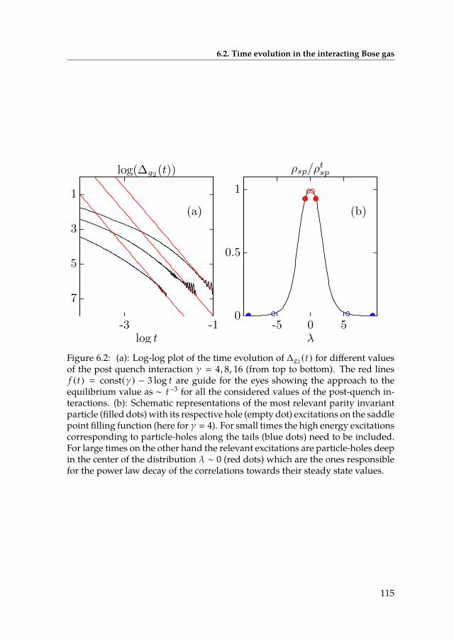
6.2. Time evolution in the interacting Bose gas
−7
−5
−3
−1
-3 -1
(a)
0
0.5
1
-5 0 5
(b)
log t
log(∆g2(t))
λ
ρsp/ρtsp
Figure 6.2: (a): Log-log plot of the time evolution of ∆g2 (t) for dierent valuesof the post quench interaction γ 4, 8, 16 (from top to bottom). The red linesf (t) const(γ) − 3 log t are guide for the eyes showing the approach to theequilibrium value as ∼ t−3 for all the considered values of the post-quench in-teractions. (b): Schematic representations of the most relevant parity invariantparticle (lled dots)with its respective hole (empty dot) excitations on the saddlepoint lling function (here for γ 4). For small times the high energy excitationscorresponding to particle-holes along the tails (blue dots) need to be included.For large times on the other hand the relevant excitations are particle-holes deepin the center of the distribution λ ∼ 0 (red dots) which are the ones responsiblefor the power law decay of the correlations towards their steady state values.
115
6. Post-quench time evolution of integrable models
The initial state is chosen to be the ground state in the absence of interactionsγ0 0, where γ c/n eectively parametrizes the coupling in the thermody-namic limit. This state is known as the Bose-Einstein condensate (BEC) state|BEC〉 and it is spatially structureless in all coordinates, 〈x|BEC〉 1
LN/2 . We con-sider the post-quench time evolution of the static density moment g2(x 0),measuring the rate of two-body inelastic processes in the gas [175] which canbe experimentally accessed through the measurement of the photoassociationrate [28]
g2(x 0, t) 〈BEC|e iHLL t : (ρ(0)/n)2: e−iHLL t|BEC〉 . (6.2.2)
The density operator is dened as ρ(x) Ψ†(x)Ψ(x), where the bosonic opera-torsΨ(x),Ψ†(x) satisfy the canonical commutation relations [Ψ(x),Ψ†(x′)] δ(x − x′). The overlaps and in particular the generalized one-particle overlapcoecient have been computed in [1]
sBEC0 (λ) log *,λc
√λ2
c2+ 14
+-, (6.2.3)
where the branch-cut of the logarithm is chosen such that sBEC0 (−λ) −sBEC0 (λ).The one-particle energy and momentum are given by k0(λ) λ and ε0(λ) λ2.The function sBEC0 (λ) determines the saddle point statewhich can be analyticallywritten in terms of Bessel functions of the rst kind In (z) [1]
ρsp(λ) −γ
4π1
1 + asp(λ)∂asp(λ)∂γ
, (6.2.4)
asp(λ) 2π/γ
λc sinh
(2πλ
c
) I1−2i λc
(4√γ
)I1+2i λc
(4√γ
).
The matrix elements between the eigenstates of the model are given in [176,177]. The sum is performed by averaging over dierent nite size realizations|λsp〉 → |ρsp〉 of the saddle point state and evaluating the relevant excitations viaan adaptation of the ABACUS algorithm [16, 143, 144] to generic highly-excitedstates. In gure 6.1 the time evolution computed via the quench action approach(6.1.10) shows that even for values of the coupling constant that are far from thetwo perturbative regimes (weak and strong coupling) we recover the initial BECvalue of the correlation limth g2(x 0, t 0+) ≡ g2(x 0)BEC 1 [175]. Thethermodynamic results allow to extract their large time decay to their steadystate values as in gure 6.2. This follows the expected t−3 law which is a conse-quence of (6.1.13) and of the behavior of sBEC0 (λ) around λ 0
exp(sBEC0 (λ 0)
) 0 ∀ γ > 0 , (6.2.5)
d exp(sBEC0 (λ)
)dλ
λ0 , 0 ∀ γ > 0 . (6.2.6)
116
6.3. Time evolution of local observables for quenches from the BEC state to hard-corebosons
This shows that the relaxation following a power law is present for any post-quench coupling constant γ, even in the limit of small interactions. This is incontrast to the predictions of the Bogoliubov approximation where the decay ispredicted to be exponential for small γ [161]. Note that the behavior of the over-lap as in (6.2.5) is also independent of the initial value of the coupling constant.It is related to the fact that for quenches from the ground state of the theory witha coupling γ0 > 0 to the gas with a nite coupling γ > 0 the eigenstate with themaximal overlap e−SΨ0λ is clearly the ground state of the nal theory. This leads tothe divergent behavior of the generalized single-particle overlap for small val-ues of the rapidity, limλ→0 e−sΨ00 (λ)
→ ∞ which leads to (6.2.5). Therefore thesame power law t−3 is expected for any interaction quench γ0 → γ inside therepulsive regime of the one-dimensional Bose gas (for the cases γ0 > 0→ γ 0see [164,178]).
6.3 Time evolution of local observables for quenchesfrom the BEC state to hard-core bosons
We consider again the Lieb-Liniger [22] Hamiltonian given by
HLL −
N∑j1
∂2
∂x2j
+ 2cN∑
j>k1δ(x j − xk ) . (6.3.1)
In the limit c → ∞ the Bethe equations for the rapidites λ become the standardquantization conditions for free fermionic momenta
limc→∞
λ j 2πI j
L. (6.3.2)
In this limit there is a rigorous one-to-one correspondence between the wavefunction and the Slater determinant for free spinless fermions [179]. The relationbetween the two is given by
limc→∞
ψ (x |λ) N∏
i< j1sgn(xi − x j )
detNi , j1(e ixiλ j
)√
N!. (6.3.3)
From now on we focus on the quench from the BEC state to the c +∞ Lieb-Liniger model. In this limit the Bethe Ansatz wave function takes the simplerform given in equation (6.3.3) and it can be integrated together with some staticphysical operators for any nite size N (see Appendix C in [1] and [180]). It isthen possible to extract the thermodynamic limit of the nite size expressionsfor the form factors. Also in this limit the back-ow is zero limc→∞ F(λ |µ) 0and as a rst consequence the dierential overlaps and the energies have much
117
6. Post-quench time evolution of integrable models
simpler expressions in terms of the rapidities of the excitations:
exp δs(µ) exp(log µ/2) µ/2 , (6.3.4)exp(−2itδω(µ)) exp(−2itµ2) . (6.3.5)
The saddle point distribution for this quench is given by [1, 156, 168]
ρsp (λ) 12π
11 + (λ/2)2
, (6.3.6)
ρhsp (λ)
12π
(1 − ρsp (λ)
)
12π
(λ/2)2
1 + (λ/2)2. (6.3.7)
6.3.1 Time Evolution of the density-density correlationsWe review here some results obtained in [1] for the two-point density-densityoperator ρ(x)ρ(0) where ρ(x) Ψ†(x)Ψ(x) and Ψ is the bosonic annihilationoperator.At c ∞ the density operator ρ connects only states which dier at most forone particle-hole. The only non-zero form factors of ρ(x)ρ(0) are then the di-agonal one and the two particle-hole ones corresponding to the rst two termsin the sum (6.1.10). The form factor for the parity-invariant two-particle holeexcitations is given by
〈ρsp |ρ(x)ρ(0) |ρsp , h ,−h → p ,−p〉 4 sin (hx) sin (px) , (6.3.8)
which is a special case of the two particle-hole form factor for generic thermo-dynamic states |ρ〉 at c ∞
〈ρ |ρ(x)ρ(0) |ρ, µ−1 , µ−
2 → µ+1 , µ
+2 〉
(e i xp1 − e i xp2
) (e−i xµ−1 − e−i xµ−2
). (6.3.9)
Combining this with the diagonal form factor
〈ρ |ρ(x)ρ(0) |ρ〉 1 + δ(x) − ˆ∞
−∞
dλρ(λ)e ixλ2, (6.3.10)
we can recover the whole time evolution summing over all these classes of pos-sible excitations
〈0(t) |ρ(x)ρ(0) |0(t)〉 〈ρsp |ρ(x)ρ(0) |ρsp〉 (6.3.11)
+ 4ˆ∞
0dhdpρsp (h)ρh
sp (p)e−2itε(p)+2itε(h)−δ(p)+δ(h) sin(px) sin(hx) ,
(6.3.12)
where we used the fact that ρ(x)ρ(0) is a self-adjoint operator to write the timeevolution only as a single sum. By substituting the expressions for the BEC
118

6.3. Time evolution of local observables for quenches from the BEC state to hard-corebosons
quench overlaps (6.3.4) we can then simplify the above expression to
〈0(t) |ρ(x)ρ(0) |0(t)〉 δ(x) + 1 − e−4|x | + 14
e2xerfc
(8it + x√8it
)− (x → −x)
2.
(6.3.13)
This reproduces the result of Ref. [168] but dierently from the method usedin there. The result can be extended easily to a generic quench protocol with agiven saddle point distribution ρsp and dierential overlaps δs. It is interestingto consider the large time behavior of the time evolution. The approach of thecorrelator to its saddle point value is indeed given by
〈0(t) |ρ(x)ρ(0) |0(t)〉 − 〈ρsp |ρ(x)ρ(0) |ρsp〉 1
512π1t
( xt
)2+ O(t−5) .
(6.3.14)
0.5
0.6
0.7
0.8
0.9
1
0 0.2 0.4 0.6 0.8 1
x
(b)
0
0.2
0.4
0.6
0.8
1
0 0.5 1 1.5 2 2.5
x
(a)
Figure 6.3: Panel (a): Time evolution of one-body density matrix〈0(t) |Ψ†(x)Ψ(0) |0(t)〉 on the time evolved BEC state ε−itHLL |0〉 |0(t)〉 as afunction of x and for given values of time t 10−3 , 5 × 10⁻³ , 10−2 , 5 × 10⁻² , 10−1(black lines) from top (t 10−3) to bottom (t 10−1) and for innite time af-ter the quench limt→∞〈0(t) |Ψ†(x)Ψ(0) |0(t)〉 e−2|x | (red dotted line). Panel(b): 〈0(t) |Ψ†(x)Ψ(0) |0(t)〉 on the interval x ∈ [0, 1] and for t 10−3(1 + 2k) fork ∈ [0, 5] (black lines) from top (k 0) to bottom (k 5).
119

6. Post-quench time evolution of integrable models
6.3.2 Time evolution of the one-body density matrixIn the following we derive an analytical expression for the time evolution of thebosonic eld-eld operatorΨ†(x)Ψ(y) (wherewe can set y 0 due to the trans-lational invariance of the initial state) at c ∞which constitutes the main resultof this section. Dierently from the density operator, Ψ† and Ψ connect statesdiering by an arbitrary number of particle-hole excitations. The computationof the full time evolution then requires to perform the whole sum in (6.1.10).The Fourier transform of the one-body density matrix gives the single particlebosonic momentum distribution function which in general is not the same asthe fermionic one and whose exact expression even for the ground state or for ageneric thermal state is rather involved [106,181].The necessary thermodynamic form factors are computed in [6], here we reporttheir expression for the parity-invariant excitations over the saddle point state|ρsp〉 :
〈ρsp |Ψ†(x)Ψ(0) |ρsp , −hi , hi → −pi , pi
ni1〉 (6.3.15)
Det(1 + K′ρsp )ndeti , j1
(W′(hi , p j ) W′(hi ,−p j )
W′(−hi , p j ) W′(−hi ,−p j )
)−Det(1 + Kρsp )
ndeti , j1
(W (hi , p j ) W (hi ,−p j )
W (−hi , p j ) W (−hi ,−p j )
),
where K and K′ are two kernels given respectively by
K(u , v) −4sin x
2 (u − v)u − v
, (6.3.16)
K′(u , v) −4sin x
2 (u − v)u − v
+ e i x2 (u+v) . (6.3.17)
The kernels W (1+Kρsp )−1K and W′ (1+K′ρsp )−1K′ are rigorously denedas solution of the following integral equations
W (u , v) +ˆ∞
−∞
dz K(u , z)ρ(z)W (z , v) K(u , v) , (6.3.18)
W′(u , v) +ˆ∞
−∞
dz K′(u , z)ρ(z)W′(z , v) K′(u , v) . (6.3.19)
Given a kernel A(u , v) and a function φ(u) we denote with Det(1 + Aφ) theFredholm determinant (see [158]) of the kernel [Aφ](u , v) A(u , v)φ(v). Wealso introduced the short-hand notation for the minor of a kernel A(u , v)
ndeti , j1
A(xi , x j ) det*..,
A(x1 , x1) A(x1 , x2) . . . A(x1 , xn )...
...A(xn , x1) A(xn , x2) . . . A(xn , xn )
+//-. (6.3.20)
120
6.3. Time evolution of local observables for quenches from the BEC state to hard-corebosons
We can then perform the sum of the rst term in (6.1.10) and nally add themirrored part. The property of the form factors under exchange of left and rightstate
〈ρ, hi → pi ni1 |Ψ
†(x)Ψ(0) |ρ〉 (〈ρ |Ψ†(x)Ψ(0) |ρ, hi → pi
ni1〉
∗) x→−x
,
(6.3.21)
allows to express the mirrored sum as the complex conjugate with x → −x ofthe rst sum. Since this is a real and symmetric function of x we can just expressthe time evolution of the one-body density matrix as a single sum
〈0(t) |Ψ†(x)Ψ(0) |0(t)〉
∞∑n0
1n!2
×
n∏j1
ˆ∞
0dµ+
j
ˆ∞
0dµ−j ρsp (µ−j )ρh
sp (µ+j )e−δs(µ+j )+δs(µ−j )−2it(δω(µ+j )−δω(µ−j ))
× 〈ρsp |Ψ
†(x)Ψ(0) |ρsp , µ−
j ,−µ−
j → µ+j ,−µ
+j
nj1〉
Det(1 + K′ρsp )∞∑
n0
1n!2
×
[ n∏j1
ˆ +∞
0dµ+
j ρhsp (p j )dµ−j ρsp (h j )e−2it(δω(µ+j )−δω(µ−j ))−δs(µ+j )+δs(µ−j ) ]
×
ndeti , j1
(W′(hi , p j ) W′(hi ,−p j )
W′(−hi , p j ) W′(−hi ,−p j )
)− (K′,W′
→ K,W ) . (6.3.22)
The product of the saddle point distribution times the dierential overlaps andenergies can be rewritten as one function for particle excitations and one forholes
ρhsp (µ)e−2itδω(µ)−δs(µ)
e−2itδω(µ)ϕ(0)+ (µ) ϕ(t)
+ (µ) , (6.3.23)
ρsp (µ)e2itδω(µ)+δs(µ) e2itδω(µ)ϕ(0)
− (µ) ϕ(t)− (µ) . (6.3.24)
Now we use the following identity [129]: consider the following multi dimen-sional integral where µ(y) is some well-dened measure on a domain X ∈ R
[ n∏α1
ˆX
dµ(yα)]
detα[1,2n],β[1,n]
(Aα (yβ) Bα (yβ)
). (6.3.25)
121
6. Post-quench time evolution of integrable models
The integration can be performed and it leads to
[ n∏α1
ˆX
dµ(yα)]
detα[1,2n],β[1,n]
(Aα (yβ)Bα (yβ)
). n!
√2ndetα,β1
aαβ n!Pf2nα,β1 (aαβ) ,
(6.3.26)
where Pf2ni , j1 is the Pfaan of the matrix aαβ and aαβ is given by
aαβ ˆ
Xdµ(y)
(Aα (y)Bβ (y) − Aβ (y)Bα (y)
). (6.3.27)
In our case we can choose Aα (yβ) W (hi , p j )(W (−hi , p j )) for odd(even) α ∈[1, . . . , 2n] andwith the same logic Bα (yβ) W (hi ,−p j ) (Bα (yβ) W (−hi ,−p j ))for odd(even) α ∈ [1, . . . , 2n]. With such a choice of the index we can integrateover the µ+
j nj1 for each n using the identity (6.3.25)
n∏j1
ˆ∞
0dµ+
j ϕ(t)+ (µ+
j )
ndeti , j1
(W (hi , p j ) W (hi ,−p j )
W (−hi , p j ) W (−hi ,−p j )
)
n! Pfni , j1
(Φ(hi , h j ) Φ(hi ,−h j )Φ(−hi , h j ) Φ(−hi ,−h j )
), (6.3.28)
where the new kernel Φ(u , v) is given by
Φ(u , v) ˆ∞
0dy ϕ(t)
+ (y)(W (u , y)W (v ,−y) −W (u ,−y)W (v , y)
)
ˆ∞
−∞
dy ϕ(t)+ (y)W (u , y)W (v ,−y) . (6.3.29)
In the last stepweused the antisymmetry of the dierential overlapswhich leadsto ϕ(t)
+ (−y) −ϕ(t)+ (y). The same can be done for the function W′ leading to an
analogous result as in (6.3.28) with a dierent kernel Φ′ given by
Φ′(u , v) ˆ∞
−∞
dy ϕ(t)+ (y)W′(u , y)W′(v ,−y) . (6.3.30)
The expression (6.3.22) then translates to
〈0(t) |Ψ†(x)Ψ(0) |0(t)〉
Det(1 + K′ρsp )∞∑
n0
1n!
n∏j1
ˆ +∞
0dµ−j ϕ
(t)− (µ−j )
× Pfni , j1
(Φ′(hi , h j ) Φ′(hi ,−h j )Φ′(−hi , h j ) Φ′(−hi ,−h j )
)− (K′,Φ′ → K,Φ) .
122
6.3. Time evolution of local observables for quenches from the BEC state to hard-corebosons
We now use the denition of the Fredholm Pfaan for the kernel Φ (which canbe equivalently implemented for the kernel Φ′)
∞∑n0
1n!
n∏j1
ˆ +∞
0dµ−j ϕ
(t)− (µ−j )
× Pfn
i , j1
(Φ(hi , h j ) Φ(hi ,−h j )Φ(−hi , h j ) Φ′(−hi ,−h j )
)
Pf(J + P0Φϕ
(t)− P0
)
√Det(I − P0 JΦϕ(t)
− P0) , (6.3.31)
where we introduced the 2 × 2 matrix kernels
Φ
(Φ++ Φ+−Φ−+ Φ−−
)J
(0 1−1 0
), (6.3.32)
where 1 denotes the identity on the kernel space as usual and the set of kernelsΦ±± are dened as Φ±± ≡ Φ(±u ,±v). The function P0 is the projector on thepositive real line x > 0. In the last step we used the relation between FredholmPfaan and Fredholm determinant Pf
(J +Φ
)2 Det(I − JΦ). The square root
of this expression produces an undetermined sign which in (6.3.31) is chosen tobe positive. This choice is purely arbitrary and its correctness is checked in thelimit t 0+ where the expression for the time evolution recovers the one-bodydensity matrix of a BEC state. The antisymmetry of ϕ(t)
− (−y) −ϕ(t)− (y) leads
to
Det(I − P0 JΦP0ϕ(t)− ) Det
(1 − P0ϕ(t)
− Φ−+P0 −P0ϕ(t)− Φ−−P0
P0ϕ(t)− Φ++P0 1 + P0ϕ(t)
− Φ+−P0
) Det(1 + ϕ(t)
− Φ+−) , (6.3.33)
where the last Fredholm determinant is dened on the whole R axis. Usingthe behaviour of W and W′ under inversion of its coordinates W (−u ,−v)
W ∗(u , v) (1 + Kρsp )−1∗K∗ (see Appendix A in [6]) the kernel Φ+− Φ(u ,−v)can be written in terms of the kernels K as the following product of operators
Φ+− Wϕ(t)+ W ∗
(1 + Kρsp )−1Kϕ(t)+ [(1 + Kρsp )∗]−1K∗ . (6.3.34)
Using the Cauchy-Binet formula for determinants we obtain
Det(1 + ϕ(t)− Φ+−) Det(1 +Φ+−ϕ
(t)− )
Det(1 + Kρsp + Kϕ(t)
+ [(1 + Kρsp )∗]−1K∗ϕ(t)− )
Det(1 + Kρsp )
Det(1 + Kρsp −Kϕ(t)
+K∗ϕ(t)
− 1 + K∗ρsp
)Det(1 + Kρsp )2
(6.3.35)
where in the last step we used the following property for the determinant of ablock matrix
det(A BC D
) detD × det(A − BD−1C) . (6.3.36)
123
6. Post-quench time evolution of integrable models
Then nally we can write the full analytical result for the time evolution valid atany time t in the thermodynamic limit
〈0(t) |Ψ†(x)Ψ(0) |0(t)〉
√Det
(1 + K′ρsp −K′ϕ(t)
+K′∗ϕ(t)
− 1 + K′∗ρsp
)−
√Det
(1 + Kρsp −Kϕ(t)
+Kϕ(t)− 1 + Kρsp
), (6.3.37)
where we used the fact that the kernel K+ K is real and symmetric and thatthe determinants of Kρsp and K′ρsp are real numbers.
The limit t → ∞ recovers the known results for the expectation value of theeld-eld operator on the saddle point state [1, 156, 168]
limt→∞〈0(t) |Ψ†(x)Ψ(0) |0(t)〉
√Det
(1 + K′ρsp 0
0 1 + K′∗ρsp
)−
√Det
(1 + Kρsp 0
0 1 + Kρsp
) Det(1 + K′ρsp ) −Det(1 + Kρsp ) ≡ 〈ρsp |Ψ
†(x)Ψ(0) |ρsp〉 e−2|x | ,(6.3.38)
where we set the kernels K∗ϕ(t)+ and K∗ϕ(t)
− to zero since for any smooth functiong on R the oscillating phase e−2it y2 sets the action of the two kernels to zero forlarge t
limt→∞
[Kϕ(t)± ]g lim
t→∞
ˆ∞
−∞
dz[Kϕ(t)± ](x , z)g(z) 0 , (6.3.39)
where the same is valid obviously also for the kernel K′.The limit t → 0+ is more involved to recover analytically but it can be evaluatednumerically as for all other values of t. We discretized the kernels in (6.3.37)with m points on the R axis reducing in this way the Fredholm determinant toa determinant of an m × m matrix as is explained in [158]. With a Gaussianquadrature method with m 800 points in the range x ∈ [−300, 300] we obtainthe expected one-body density matrix for a BEC state at t 0
〈0|Ψ†(x)Ψ(0) |0〉 1 + ε , (6.3.40)
with a constant numerical error ε ∼ 10−3. From the same numerical procedurewe obtain also the following analytical guesses for the Fredholm determinant ofthe two kernels (up to the numerical precision of the evaluation procedure)
Det(1 + Kρsp ) e−2|x | cos 2x , (6.3.41)Det(1 + K′ρsp ) e−2|x | (cos 2x + 1) . (6.3.42)
124

6.3. Time evolution of local observables for quenches from the BEC state to hard-corebosons
We used the same numerical procedure to obtain the plots in Fig 6.3 for dierentvalues of t and x.The limit x → 0 gives the density of the gas D and it is also easily recovered forany time t since K → 0 and K′ → 1. We then obtain
〈0(t) |Ψ†(0)Ψ(0) |0(t)〉
√Det
(1 + ρsp −ϕ(t)
+ϕ(t)− 1 + ρsp
)− 1
√√Det
(e−itδω 0
0 e itδω
) (1 + ρsp −ϕ(0)
+ϕ(0)− 1 + ρsp
) (e−itδω 0
0 e itδω
)−1 − 1
√Det
(1 + ρsp −ϕ(0)
+ϕ(0)− 1 + ρsp
)− 1
√(1 +ˆ∞
−∞
dλρsp (λ))2
+(ˆ∞
−∞
dλϕ(0)+ (λ)
)2− 1
D , (6.3.43)
where in the last steps we used that ϕ(0)+ (λ) ϕ(0)
− (λ) and ϕ(0)+ (λ) −ϕ(0)
+ (−λ).Furthermorewe extended the followingproperty of the determinant (with v j
Nj1
and c j Nj1 two dierent vectors)
det2N
(δi j + v j −c j
c j δi j + v j
)
*.,1 +
N∑j1
v j+/-
2
+ *.,
N∑j1
c j+/-
2
, (6.3.44)
to the Fredholm determinant in (6.3.43).Approach to equilibrium for large times after the quenchWe show here that the leading contribution to the time evolution, given by equa-tion (6.3.37), for large time is only given by the parity-invariant 2 particle-holeexcitations, namely what we introduced in formula (6.1.12). In order to showthat we start from formula (6.3.33) and we expand it for large time t
Det(1 + ϕ(t)− (y)Φ+−) , (6.3.45)
where
Φ+−(u , v) ˆ
dyϕ(t)+ (y)(y)W (u , y)W ∗(v , y)
ˆdyπ
ye−2it y2
4 + y2 W (u , y)W ∗(v , y).
(6.3.46)
125

6. Post-quench time evolution of integrable models
The procedure to follow is simply to extract the saddle point for large t of the in-tegral over y. This is given by y 0. Therefore we need to expand the integrandaround y 0
W (u , y)W ∗(v , y) W (u , 0)W ∗(v , 0)(1 + (g(u) + g∗(v))y
). (6.3.47)
Therefore we obtain for the kernel Φ+−(u , v)
Φ+−(u , v) →W (u , 0)W ∗(v , 0)14π
ˆdye−2i y2t y2
14π
√π2
4(−it)3/2W (u , 0)W ∗(v , 0)
(g(u) + g∗(v)
). (6.3.48)
To determine the function g(u) we need to take the kernel W and expand it onthe second variable
W (u , v) +ˆ
dsK(u , s)ρsp (s)W (s , v) K(u , v) , (6.3.49)
W (u , v) +ˆ
dsK(u , s)ρsp (s)W (s , v)
K(u , 0)(1 +
v(iu2xe
iux2 −
82 (sin(ux)) + 4
2ux(cos(ux)))
−82u(sin(ux)) + 2u2e
iux2
).
(6.3.50)
We have then
W (u , v) W (u , 0) + g(u)v , (6.3.51)
where
g(u)+ˆ
dsρsp (s)K(u , s)g(s) K(u , 0)( (iu2xe
iux2 −
82 (sin(ux)) + 4
2ux(cos(ux)))
−82u(sin(ux)) + 2u2e
iux2
).
(6.3.52)
We can now use the following property of determinants
det(δi j + αci f j (vi + v j )) 1 + 2α∑
ci fi vi + O(α2) , (6.3.53)
126
6.3. Time evolution of local observables for quenches from the BEC state to hard-corebosons
which allows to expand the Fredholm determinant as
Det(1 + ϕ(t)− (y)Φ+−)
Det(1 + 2 1
4π
√π2
4(−it)3/2ϕ(t)− (y)(u)W (u , 0)W ∗(v , 0)<g(u)
) 1 + 2 1
4π
√π2
4(−it)3/2
ˆdu |W (u , 0) |2<g(u)ϕ(t)
− (y)(u) (6.3.54)
We can now expand again the integral around its saddle point for large t
|W (u , 0) |2<g(u) |W (0, 0) |2<g(0) + u[∂u |W (u , 0) |2<g(u)u0] (6.3.55)
Finally we report the leading contribution for large time of the one-body densityfunction
〈0(t) |Ψ†(x)Ψ(0) |0(t)〉 ∼ e−2x+
1t3
( 14π
√π2
4)2 (
Det(1 + K′ρsp )[∂u |W′(u , 0) |2<g2(u)u0
]
−Det(1 + Kρsp )[∂u |W (u , 0) |2<g(u)u0
] )(6.3.56)
with
g2(u) +ˆ
dsρsp (s)K(u , s)g2(s) 2ux cos(ux/2) − 4 sin(ux/2)
u2 + 12 ixe
iux2
(6.3.57)
g(u) +ˆ
dsρsp (s)K(u , s)g(s) 2ux cos(ux/2) − 4 sin(ux/2)
u2 (6.3.58)
Note that this can also be rewritten as the saddle point of the following integrals
〈0(t) |Ψ†(x)Ψ(0) |0(t)〉 ∼ e−2x
+ Det(1 + K′ρsp )(1 + 1
2
ˆ∞
−∞
duˆ∞
−∞
dyϕ(t)+ (y)(y) |W′(u , y) |2ϕ(t)
− (y)(u))
− (W′→W ) (6.3.59)
which is the same as the two particle-hole contribute of sum (6.3.22). These twoparity invariant particle-hole excitation (whose momentum spams on the realline [0, +∞]) can be written as an eective single particle-hole excitation withmomenta on thewhole real line as in equation (6.3.59).We have therefore showedthat the late time dynamics of the correlation function is only given by an eec-tive one particle-hole excitation on the saddle point state.
127
6. Post-quench time evolution of integrable models
Time evolution of the momentum distributionThe Fourier transform of the one-body density matrix gives the momentum dis-tribution of the gas
nt (k) 12π
ˆ∞
−∞
dyˆ∞
−∞
dxe ik(x−y)〈0(t) |Ψ†(x)Ψ(y) |0(t)〉 . (6.3.60)
This is a muchmore relevant quantity from the experimental point of view sinceit can be directly accessed by releasing the trap for the gas and measuring theposition of the atoms after they have ied freely in the experimental chamber.As is visible in gure 6.3 the gas keeps a long range correlation
limx→∞〈0(t) |Ψ†(x)Ψ(0) |0(t)〉 C(t) (6.3.61)
for any time after the quench, with C(t) ∼ t−3. Therefore the momentum dis-tribution at any time has a nite part and a condensate at k 0 formed by anumber NC(t) of particles
nt (k) C(t)δ(k) + n (0)k (k) . (6.3.62)
As shown in gure 6.4, the function relaxes quite quickly to its equilibrium valuegiven by
n∞(k) 12π
11 + (k/2)2
. (6.3.63)
128

6.3. Time evolution of local observables for quenches from the BEC state to hard-corebosons
-20 -10 10 20
0.05
0.10
0.15
Figure 6.4: Time evolution of the nite part of the momentum distributionn (0)
t (k) as a function of momentum πk/kF (black lines) for t sdt, s 0, 1, . . . , 5and dt 0.002 (from bottom to top). The blue line represents the momentumdistribution of the steady state. The momentum is relaxed for almost all the k att ∼ 0.01 which for a gas of 87Rb at density n ∼ 106/m corresponds to 10−6s.
129

CHAPTER 7
Néel quench in the XXZ spin chain
Et tu, Brute?
Caesar in Julius Caesar,W. Shakespeare
This chapter focuses on expectation values of local spin-spin operators after therelease of the zero momentum Néel state
|Ψ0〉 1√2
(| ↑↓ . . . ↑↓〉 + | ↓↑ . . . ↓↑〉) (7.0.1)
into a XXZ spin chain with anisotropy ∆ ≥ 1. For these values of ∆ the spec-trum of the Hamiltonian is gapped, except at the point ∆ 1, when the gapcloses. Formally it corresponds to performing an interaction quench from theground state of the theory with ∆0 +∞ to the model with a nite ∆. The ex-act overlaps computed in section 3.2 allow to directly apply the quench actionmethod, which corresponds to exactly compute the diagonal ensemble of thequench in the thermodynamic limit. As a lattice model it has a well denedultra-violet cut-o, dierently from the Lieb-Liniger model, and the expecta-tion values of the conserved charges Qm
∞
m1 on the initial state, as well as theiructuations∆Qm are all well-dened. Therefore a GGE prediction for the expec-tation values of local observables in the steady state can then be extracted. Thecomparison between the two approaches shows that a GGE ensemble includ-ing all the local conserved charges enforcing integrability (the ones introducedin (2.3.22)) does not x properly the late times expectation values of local op-erators. This is expected to be a generic feature of the GGE ensemble for anyquench in the XXZ model when the initial state has a nite extensive energydensity 〈Ψ0 |H |Ψ0〉 ∼ Ne0.
We rst introduce the string solutions (bound states) of the Bethe equations forthe XXZmodel (section 7.1), necessary to extend the thermodynamic descriptionof the eigenstates as done for the Lieb-Linigermodel in section 4.2. Thenwe givean example of a correlation function of a local operator in the thermodynamiclimit (section 7.2) as a function of the densities of rapidites ρn (λ) describing thethermodynamic state. We can thenmove to the quench from theNéel initial stateand compare the prediction of the quench action approach (section 7.4) with theone of the GGE ensemble built with local charges (section 7.3).
131

7. Néel quench in the XXZ spin chain
This chapter is based on the results published in [4, 5].
7.1 Thermodynamic Bethe Ansatz for the XXZ spinchain
The XXZ model was introduced in 3.2.1. The Bethe equations for the rapiditesλ λ j
Nj1 read( sin(λ j + iη/2)
sin(λ j − iη/2)
)N
−
M∏k1
sin(λ j − λk + iη)sin(λ j − λk − iη)
, j 1, . . . ,M . (7.1.1)
where η is related to the anisotropy ∆ by ∆ cosh η. The solutions of theseequations are not all real numbers as it is the case for the repulsive Lieb-Linigermodel. In fact they form pattern in the complex plane in the form of strings
λ j λnα + ic/2( j + 1 − 2a) + δa
n ,α , a 1, . . . , n . (7.1.2)
For most of the strings in each state the deviations δan ,α vanish exponentially
for large system size δan ,α ∼ e−Lαa
n ,α and therefore we can safely assume, forlarge enough system size that all the solution of the Bethe equations are per-fect strings (rapidities disposed as in (7.1.2) with deviations set to zero δa
n ,α 0).However some of the strings have deviations that decay as power laws ∼ 1/Nα
and for such states taking the limit of zero deviation δ → 0 requires particularcare. On the other hand we are interested in thermodynamic properties of themodel and therefore we can focus only on a class of states which has only perfectstrings and that is suciently large to reproduce most of the quantities we areinterested in 1. It has been shown indeed that considering only states with per-fect string rapidities reproduces the thermodynamic limit at xedmagnetizationlimth M/N
12 − 〈σ
z〉 and xed temperature T (the so called string hypothesis
[182]). This means that we can consider only states with perfect strings and re-produce thermodynamic results for any ∆. This will be our working hypothesisalso for post-quench situations.Under the string hypothesis a state is solely characterized by its real string cen-ters λn
αα,n . The logarithmic form of the Bethe Eqs (3.2.6) can be recast into theBethe-Gaudin-Takahashi (BGT) equations for string centers [107,183,184],
θn(λnα)
2πN
Inα + 1
N
∑(m ,β) ,(n ,α)
θnm(λnα − λ
mβ
)(7.1.3a)
for n ≥ 1 and α 1, 2, . . . ,Mn . Here,
θnm (λ) (1−δnm )θ|n−m | (λ)+2θ|n−m |+2(λ)+. . .+2θn+m−2(λ)+θn+m (λ) (7.1.3b)
1In other words, given a local observable O and the set of states with perfect strings |λδ0〉, theresolution of identity is valid up to nite size corrections
∑λδ0 O |λδ0〉〈λδ0 | O(1 + O(1/N)))
132

7.1. Thermodynamic Bethe Ansatz for the XXZ spin chain
and
θn (λ) 2 arctan *,
tan(λ)tanh( nη
2 )+-. (7.1.3c)
Note that the function θ2 is the scattering phase shift. The quantum numbers Inα
are as usual integers (half-odd integers) if N −Mn is odd (even).We can straightforwardly generalize our way of introducing a thermodynamicBethe state as done in 4.1 simply moving from the complex rapidities λi
Mi1 to
the set of real string centers λnα
Mnα1 where Mn is the number of strings with
length n, such that∑n
Mn M (7.1.4)
where the sum runs over all the string lengths present in the state. In the gappedregime, when ∆ ≥ 1 all the string lengths are allowed (in the gapless −1 < ∆ < 1there are some forbidden string lengths depending on the value of∆) and due tothe periodicity of the scattering kernel we can reduce the domain of the rapidi-ties to the Brillouin zone −π/2 < λn
α < π/2. For thermodynamic purposes weneglect all the states which contain strings with an extensive n ∼ M dimen-sion and we impose that the lenghth of the largest string is o(M), such thatlimth o(M)/M 0. The generalization of equation (4.1.10) reads
ρn ,t (λ) an (λ) −∞∑
m1(anm ∗ ρm )(λ) (7.1.5a)
for n ≥ 1, where ρn ,t (λ) ρn (λ) + ρn ,h (λ) and ρn ,h is the hole density of n-strings. Further,
anm (λ) (1−δnm )a |n−m | (λ)+2a |n−m |+2(λ)+ . . .+2an+m−2(λ)+an+m (λ) (7.1.5b)
with
an (λ) 12π
ddλθn (λ)
1π
sinh(nη)cosh(nη) − cos(2λ)
. (7.1.5c)
The convolution is dened by
( f ∗ g) (λ) ˆ π/2
−π/2dµ f (λ − µ) g(µ) . (7.1.6)
For both numerical and analytical evaluation of the integral equations, it is of-ten convenient to get rid of the innite sum over string types and to work withthe “partially decoupled” set of equations. The partially decoupled form of thethermodynamic BGT equations can be derived [174],
ρn (1 + ηn ) s ∗ (ηn−1ρn−1 + ηn+1ρn+1) (7.1.7a)
133

7. Néel quench in the XXZ spin chain
for n ≥ 1, where the λ-dependence is left implicit and we use the conventionsη0(λ) 1 and ρ0(λ) δ(λ). The kernel in Eqs (7.1.7a) reads
s(λ) 12π
∑k∈Z
e−2ikλ
cosh(kη). (7.1.7b)
For each string length n 1, 2, . . . we can divide the real line into Nnb boxes
with llings ϑnk with k 1, . . . ,Nn
b . Our (themrodynamically exact) resolutionof identity (4.1.13) therefore generalizes to
1H
o(M)∏n1
*.,
Nnb∏
k1
1∑ϑn
k 0
∑cn
k
+/-
∑en
k
|ϑnk , c
nk , e
nk 〉〈ϑ
nk , c
nk , e
nk | (7.1.8)
The sums over the lling fractions and the particle-hole rearrangements of allthe string lengths n are then factorized in each string, which leads to generalize(7.1.9) to
limth
nmax∏n1
*.,
Nnb∏
k1
1∑ϑn
k 0
∑cn
k
+/-
∑en
k
ˆ ∞∏n1
[Dϑn eSYY [ϑn ]
] ∑ek
n
(7.1.9)
where nmax ∼ o(M). Note that now the sum over the non-extensive excitations∑ek
n not only involves particle-hole creations within strings of the same lengths
but also a non-extensive number of strings creation-annihilation (for example:two strings of length n 1 which are transformed into a single string of lengthn 2). We can denote the set of lling functions ϑn (λ)(as well as the distri-bution ρn (λ), ρn ,h (λ)) with vectors of functions ϑ, ρ and ρh . Note also that itis coveninent to switch from the basis of lling functions ϑ to the basis given bythe functions η
ρhρ . With this notation the free energy of a XXZ spin chain in
the gapped regime ∆ > 1 is easily expressed in the thermodynamic limit as thesaddle point of the following integral
F(β) −β log∑λ
e−βE[λ] −β log
ˆdh
ˆ ∞∏n1
[Dηn e−βN
´dλρn (λ)(−π J sinh(η)an (λ))+SYY [ηn ]+βhN (n
´dλρn (λ)−M)
]+ const.
(7.1.10)
where
SYY[ηn] ˆ π/2
−π/2dλ
[ρn ln(1 + ηn ) + ρn ,h ln(1 + η−1n )
]. (7.1.11)
134

7.2. An example of thermodynamic correlation function: nearest-neighborscorrelation function
This leads to a set of an innite number of coupled integral equations for thefunctions η
log ηn (λ) β(−π J sinh(η)an (λ) + 2nh) +∞∑
m1(anm ∗ log(1 + η−1m ))(λ)
(7.1.12)
The solution of these equations gives the free energy of a gapped XXZ spin chainat nite temperature T
F N∞∑
n1
ˆ π/2
−π/2dλ ρn (λ)(−π J sinh(η)an (λ) + 2nh)
+ β−1(ρn (λ) log(1 + ηn (λ)) + ρn ,h (λ) log(1 + η−1n (λ))
)(7.1.13)
where the density of holes ρn ,h are related to the densities ρn by the Bethe equa-tions (7.1.7a).
Not only the free energy can be obtained but any correlation function at nitetemperature can be in principle obtained by the set of solution η (as for the Lieb-Liniger we can in principle write any correlation function as a functional of thelling function ϑ(λ) (4.3.19)). The expression of only η for a generic thermody-namic correlation function 〈η|σ jσ j+l |η〉 is hard to obtain (one has to perform asum over all the eigenstates in 4.3 for the Lieb-Liniger) but some simple nearest-neighbours correlations can be easily computedwith theHellman-Feynman the-orem or some special symmetries of the chain. This will be the topic of the nextsection.
Finally we conclude that what we have done here for the thermal case can begeneralized trivially to any driving term e−βH
→ e−F like for example the gen-eralized Gibbs measure for quenches (see section 7.3) FGGE
∑n βnQn or the
driving term of the quench action approach FQ −2 limth< log〈Ψ0 |λ〉 (see sec-tion 7.4).
7.2 An example of thermodynamic correlation func-tion: nearest-neighbors correlation function
The operator σzj σ
zj+1 can be easily obtained just by dierentiating the Hamilto-
nian (2.3.24) respect to ∆, namely using the Hellmann-Feynman theorem [185]〈σz
j σzj+1〉 1 + 4
N J
⟨∂H∂∆
⟩. A naive application of the Hellmann-Feynman theorem
on the thermodynamic Bethe state leads to a meaningless result
〈η|1N∂H∂∆|η〉 ,
∂∂∆〈η|
1N
H |η〉 ∞∑
n0
ˆ π/2
−π/2dλ
∂∂∆
(−π J sinh(η)an (λ))ρn (λ)
135

7. Néel quench in the XXZ spin chain
(7.2.1)
The reason of this mismatch is due to the scaling of the overlaps of two Bethestates with dierent values of ∆ which are exponentially small in system size.This makes the thermodynamic limit and the derivative with respect to ∆ noninterchangeable,
limδ→0
limth〈λ(∆) |λ(∆ + δ)〉 , limth limδ→0〈λ(∆) |λ(∆ + δ)〉 . (7.2.2)
In order to apply theHellmann-Feynman theoremwe need to take the derivativeof the energy eigenvalue of a generic Bethe state at nite size N and then takethe thermodynamic limit. Under the string hypothesis the energy eigenvalue ωλbecomes a function only of the string centers for a large (but nite) system sizeM,
ωλ −π J sinh(η)∑n ,α
an (λnα) , (7.2.3)
We can now apply the Hellmann-Feynman theorem to this nite size state bytaking the derivative of the energy with respect to ∆:
〈λ |σz1σ
z2 |λ〉 1 + 4
N Jdωλd∆
1 + 4N J
1sinh η
dωλdη
1 − 4πN
∑n ,α
[cosh ηsinh η an (λn
α) + (∂ηan )(λnα) + ∂λn
αan (λn
α)dλn
α
dη
]. (7.2.4)
The quantities dλnα
dη are obtained by deriving the reduced Bethe equations forstring centers [99, 183]
θn (λnα) −
1N
∑m ,β
θnm (λnα − λ
mβ )
2πN
Inα (7.2.5)
with respect to the interaction parameter η,
N an (λnα) −
∑m ,β
anm (λnα − λ
mβ ) +
∑m ,β
G(n ,α),(m ,β)
dλmβ
dη 0 . (7.2.6)
Here we introduced the reduced Gaudin matrix for string centers [186]
G(n ,α),(m ,β) δ(n ,α),(m ,β)(N an (λn
α)−∑k ,γ
ank (λnα −λ
kγ)
)+ anm (λn
α −λmβ ) (7.2.7)
and the functions an and anm ,
an (λ) 12π∂ηθn (λ) −an (λ)
n sin 2λ2 sinh nη
, (7.2.8)
136
7.3. The GGE for a generic quench in the XXZ model
anm (λ) 12π∂ηθnm (1−δnm ) a |n−m | (λ)+2a |n−m |+2(λ)+. . .+2an+m−2(λ)+an+m (λ).
(7.2.9)
We dene a set of the auxiliary functions h hn ∞
n1 such that
hn (λnα)
∑m ,β
(G−1)(n ,α),(m ,β)(N am (λm
β ) −∑k ,γ
amk (λmβ − λ
kγ)
). (7.2.10)
In the thermodynamic limit, expression (7.2.4) can then be recast as a functionalof the distributions ρ(η) and the auxiliary functions h,
〈η|σz1σ
z2 |η〉 1−4π
∞∑n1
ˆ π/2
−π/2dλ ρn (λ)
[cosh ηsinh η an (λ) + ∂ηan (λ) − (∂λan (λ))hn (λ)
],
(7.2.11)
where the auxiliary functions are determined by a set of linear integral equations
ρn ,t (λ)hn (λ) +∞∑
m1anm ∗ (ρm hm ) (λ) an (λ) −
∞∑m1
anm ∗ ρm (λ) . (7.2.12)
To obtain the next nearest-neighbors correlations the process is more compli-cated [187]. One needs to use special symmetries of the XXZ spin chain that havebeen rst used in the context of the Quantum Transfer Matrix approach [188].Then, using amapping from this approach to the Thermodynamic Bethe Ansatz[189] one can write a functional representation for the correlations 〈η|σz
1σz3 |η〉
and 〈η|σz1σ
z4 |η〉.
7.3 The GGE for a generic quench in the XXZmodelAs already introduced before, given a quench protocol, the GGE approach todetermine the long time post-quench expectation values of local operators relieson the possibility of constructing such an ensemble
ZGGE Tr[e−
∑n1 βn Qn
](7.3.1)
where the chemical potentials βn have to be determined by xing the expecta-tion values of the charges on the initial state |Ψ0〉. In order to have an extensiveGeneralized Gibbs driving term
∑n1 βnQn (only an extensive functional can be
a non-trivial constraint for the entanglement entropy of the post-quench reduceddensitymatrix, see section 2.1) we focus on the rst o(M) extensive local charges
137
7. Néel quench in the XXZ spin chain
obtained from the rst derivatives of the logarithm of the transfer matrix (2.3.22)
Qk isinhk η
2k
∂k
∂µklog τ(µ)µiη/2
k 1, 2, . . . , o(M) . (7.3.2)
Higher order charges with k ∼ M are not local since they are extensive sumof operators acting non-trivially on a nite sub-region of the whole system andtherefore are not expected to inuence the out-of-equilibrium dynamics of localoperators 2. The charges Qn
o(M)n1 are then the local charges enforcing integra-
bility in the system (see section 2.1) and therefore one can naively expect thatthey provide a complete set of constraints to the GGE density matrix (7.3.1).
Finding the chemical potentials βn is a very complicated non-linear problem.Let us consider the thermodynamic Bethe state obtained from the saddle pointof the GGE ensemble (7.3.1), then the set ηGGE is obtained by maximizing theentropy under the constraints
limth〈Ψ0 |Qm |Ψ0〉
N
∞∑n1
ˆ π/2
−π/2dλ ρGGE
n (λ) c (n)m (λ) ∀m 0, 1, 2, . . . , (7.3.3)
where c (n)m (λ) is the single-particle eigenvalue of the extensive conserved charge
Qm (for example c (n)1 (λ) ∼ an (λ) which is the single-particle energy eigenvalue
for a string of length n). Luckily it turns out that the set of initial expectationvalues of the local conserved charges Qm
∞
m1 limthQm o(M)m1 has a one-to-one
correspondencewith the density ρ1,h of 1-string holes. Therefore theGGEdistri-butions ηGGE are dened as the onesmaximizing the entropywith the constraintρGGE1,h ρΨ0
1,h where ρΨ01,h is xed by the expectation values of the local charges on
the initial state.
In order to show this let us rst introduce a convention for the Fourier transform
f (k) FT[
f](k)
ˆ π/2
−π/2dλe2ikλ f (λ) , k ∈ Z , (7.3.4a)
f (λ) FT−1[
f](λ)
1π
∑k∈Z
e−2ikλ f (k) , λ ∈ [−π/2, π/2) . (7.3.4b)
2Another argument supporting the truncation of the GGE ensemble up to the rst o(M) chargesis the study of the truncated ensemble with dierent number of charges Qk
nk1 with n 2, 3, . . ..
This shows that the GGE predictions for this initial state and for local spin-spin operators acting on` spins are already converged by including a number n ∼ ` of conserved charges [76]
138
7.3. The GGE for a generic quench in the XXZ model
For m ≥ 1 the partial integration (m − 2 times) gives a simple expression for theFourier transform of c (n)
m ,
c (n)m (k) −2π
sinhm (η)2m (2ik)m−1
ˆ π/2
−π/2dλ e2ikλ an (λ)
−π sinhm (η) (ik)m−1 e−|k |nη , (7.3.5)
where we used that the Fourier transform of the XXZ kernel an in Eq. (7.1.5c) ise−|k |nη. The eigenvalue of charge Qm can then be rewritten as
∞∑n1
ˆ π/2
−π/2dλ ρΨ0
n (λ) c (n)m (λ)
1π
∞∑n1
∑k∈Z
ρΨ0n (k) c (n)
m (k)
− sinhm (η)∑k∈Z
(ik)m−1∞∑
n1ρΨ0
n (k) e−|k |nη .
(7.3.6)
The key point is now that we can perform the sum in (7.3.6) and rewrite the sumover all string densities in terms of ρΨ0
1,h only,
∞∑n1
ρΨ0n (k) e−|k |nη
e−|k |η − ρΨ01,h (k)
2 cosh(kη). (7.3.7)
This identity (whichwas obtained already for the energy of the state in [107]) canbe derived from the Fourier transform of the partially decoupled form (7.1.7) ofthe BGT equations, which is (using the convolution theorem)
ρΨ0n ,t (k)
12 cosh(kη)
[ρΨ0
n−1,h (k) + ρΨ0n+1,h (k)
](7.3.8)
for n ≥ 1, where ρΨ00,h (k) 1. The one-to-one correspondence between the ex-
pectation values of the charges Qm ∞
m2 and ρΨ01,h is thus given by
limth
(〈Ψ0 |Qm |Ψ0〉
N sinhm (η)
)
∑k∈Z
ρΨ01,h (k) − e−|k |η
2 cosh(kη)(ik)m−1 , (7.3.9)
where it should be noted that this equation holds for all m ≥ 1 and that thetotal-momentum charge is excluded.We stress that the result (7.3.9) is general, the 1-string hole density ρΨ0
1,h of thesteady state after any quench to the spin-1/2 XXZ chain is completely deter-mined by the initial values of the local conserved charges Qm
∞
m1. Note thatthe sum in Eq. (7.3.9) is quickly converging due to the exponentially decayingfactor for η > 0, which ensures invertibility.
139
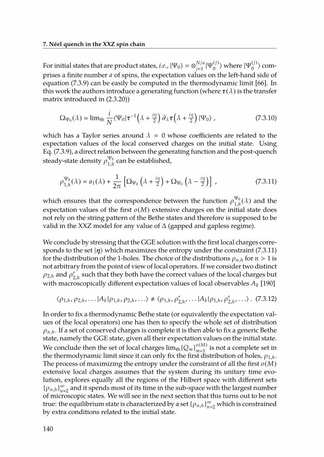
7. Néel quench in the XXZ spin chain
For initial states that are product states, i.e., |Ψ0〉 ⊗N/aj1 |Ψ
( j)0 〉where |Ψ( j)
0 〉 com-prises a nite number a of spins, the expectation values on the left-hand side ofequation (7.3.9) can be easily be computed in the thermodynamic limit [66]. Inthis work the authors introduce a generating function (where τ(λ) is the transfermatrix introduced in (2.3.20))
ΩΨ0 (λ) limthi
N〈Ψ0 |τ−1
(λ + iη
2
)∂λτ
(λ + iη
2
)|Ψ0〉 , (7.3.10)
which has a Taylor series around λ 0 whose coecients are related to theexpectation values of the local conserved charges on the initial state. UsingEq. (7.3.9), a direct relation between the generating function and the post-quenchsteady-state density ρΨ0
1,h can be established,
ρΨ01,h (λ) a1(λ) + 1
2π[ΩΨ0
(λ + iη
2
)+ΩΨ0
(λ −
iη2
)], (7.3.11)
which ensures that the correspondence between the function ρΨ01,h (λ) and the
expectation values of the rst o(M) extensive charges on the initial state doesnot rely on the string pattern of the Bethe states and therefore is supposed to bevalid in the XXZ model for any value of ∆ (gapped and gapless regime).
We conclude by stressing that theGGE solutionwith the rst local charges corre-sponds to the set |η〉 which maximizes the entropy under the constraint (7.3.11)for the distribution of the 1-holes. The choice of the distributions ρn ,h for n > 1 isnot arbitrary from the point of viewof local operators. Ifwe consider twodistinctρ2,h and ρ′2,h such that they both have the correct values of the local charges butwith macroscopically dierent expectation values of local observables Ak [190]
〈ρ1,h , ρ2,h , . . . |Ak |ρ1,h , ρ2,h , . . .〉 , 〈ρ1,h , ρ′
2,h , . . . |Ak |ρ1,h , ρ′
2,h , . . .〉 . (7.3.12)
In order to x a thermodynamic Bethe state (or equivalently the expectation val-ues of the local operators) one has then to specify the whole set of distributionρn ,h . If a set of conserved charges is complete it is then able to x a generic Bethestate, namely the GGE state, given all their expectation values on the initial state.We conclude then the set of local charges limthQm
o(M)m1 is not a complete set in
the thermodynamic limit since it can only x the rst distribution of holes, ρ1,h .The process of maximizing the entropy under the constraint of all the rst o(M)extensive local charges assumes that the system during its unitary time evo-lution, explores equally all the regions of the Hilbert space with dierent setsρn ,h
∞
n2 and it spends most of its time in the sub-space with the largest numberof microscopic states. We will see in the next section that this turns out to be nottrue: the equilibrium state is characterized by a set ρn ,h
∞
n2 which is constrainedby extra conditions related to the initial state.
140
7.4. The quench action approach to the Néel quench and the (apparent) failure of theGGE
7.4 The quench action approach to the Néel quenchand the (apparent) failure of the GGE
We focus now on the initial state |Ψ0〉 given by the zero momentum Néel state
|Ψ0〉 1√2
(|↑↓↑↓ . . .〉 + |↓↑↓↑ . . .〉) . (7.4.1)
With an expression for the GGE ensemble at hand we can wonder if this is thesame or dierent than the result given by the quench action approach. Namely,given a local observable O we want to know if the prediction given by the GGEwith the rst o(M) charges is the same as the diagonal ensemble
´Dη e−
∑n βn 〈η|Qn |η〉+SYY [η]〈η|O |η〉
ZGGE
?
limth∑λ
〈Ψ0 |λ〉2〈λ |O |λ〉
| |Ψ0 | |2
´Dη e−SQ [η]
〈η|O |η〉| |Ψ0 | |2
(7.4.2)
where the quench action SQ[η] for the Néel initial state is given analogouslyas in Lieb-Liniger (5.3.1). The dierence with the situation in here is that theoverlaps are given by the thermodynamic limit of (3.2.16) and the rapidites aresubstituted with perfect strings
SQ[η]/N
∞∑n0
[−
ˆ π/2
−π/2dλ ρn (λ)sNéel
0(n) (λ) + SYY[ηn]
], (7.4.3)
where the coecients sNéel0
(n) (λ) are the generalized single-particle overlap co-ecients for the n−th string obtained from the thermodynamic limit of the nitesize overlap (3.2.16) (performed analogously aswhat is done for the BEC to Lieb-Liniger overlaps in section 5.2). We obtain
sNéel0
(n) (λ) n∑
a1sNéel0 (λ + iη/2(n + 1 − 2a)) , (7.4.4)
where sNéel0 (λ) 1
4 log( tan(λ+iη/2) tan(λ−iη/2)
sin(2λ)2
). We obtain then
sNéel0
(n) (λ) gn (λ) + 2n ln(4) , (7.4.5)
with
gn
n−1∑l0
ln[ sn−1−2l cn−1−2l s−n+1+2l c−n+1+2l
tn−2l t−n+2l
], (7.4.6)
tn sn
cn, sn (λ) sin
(λ + iηn
2
), cn (λ) cos
(λ + iηn
2
). (7.4.7)
141
7. Néel quench in the XXZ spin chain
Coming back to question (7.4.8) it turns out that the saddle point of the integralon the left hand side (GGE) and the one on the right (quench action) are twodierent sets η. Namely
´Dη e−
∑n βn 〈η|Qn |η〉+SYY [η]〈η|O |η〉
ZGGE 〈ηGGE |O |ηGGE〉 (7.4.8)
´Dη e−SQ [η]
〈η|O |η〉| |Ψ0 | |2
〈ηsp |O |ηsp〉 (7.4.9)
with ηGGE , ηsp . This translates into two dierent predictions for the correla-tion functions of local operators (gure 7.2 and 7.3). The only shared feature isthe distribution of the 1-holes ρNéel
1,h ρGGE1,h ρ
sp1,h where ρNéel
1,h is xed by theexpectation values of all the o(M) local charges as in equation (7.3.11)
ρNéel1,h (λ)
π2a31 (λ) sin2(2λ)
π2a21 (λ) sin2(2λ) + cosh2(η). (7.4.10)
The fact that the quench action solution ηsp allows for the relation ρsp1,h ρNéel
1,hto be satised is a non-trivial check that the solution is actually correct since itreproduces the correct expectation values of the conserved charges. Moreoversince the quench action approach is based on rst principles and does not relyon any assumption it must give the correct answer (another conrmation of itscorrectness comes also from an independent numerical simulation, see gure7.3).
One may notice that the zero momentum Néel state does not obey the clusterdecomposition, therefore the uctuations of some of the local charges Qm arenot subleading for large system sizes
∆Qm
N
√〈Ψ0 |Q2
m |Ψ0〉 − 〈Ψ0 |Qm |Ψ0〉2
N→ const . (7.4.11)
However this is a mild feature of the initial state which is the ground state ofthe theory when ∆ ∞. We can imagine to perform a similar quench choosingas initial state |Ψ0〉 the ground state of the model with 1 ∆0 < ∞ which in-deed satises the cluster decomposition. Also in this quench the local chargesis an incomplete set of constraints since they x only the distribution ρ1,h of thesaddle point state as in equation (7.3.11), while thematrix elements depend non-trivially on all the other distributions of holes ρh ,n with n > 1. Therefore we canconclude that the GGE ensemble with the rst o(M) extensive local charges willfail to reproduce the exact steady state for any quench ∆0 → ∆ with ∆0 ,∆ > 0(the case ∆ 0 has not such issue since there are no bound states, namely theeigenstate are parametrized in the thermodynamic limit by a single continuous
142

7.4. The quench action approach to the Néel quench and the (apparent) failure of theGGE
function). In other words, the entropy of the GGE ensemble is too large andmore constraints are needed, namely more conserved charges have to be takeninto account in order to reproduce the correct steady state. We are then left withan impasse, where we know that there must be more conserved charges thatdo inuence the out-of-equilibrium dynamics but we do not know how to ndthem. It is a common belief that all the symmetries of the system are containedin the transfer matrix τ(λ) of equation (2.3.22) which indeed gives a completeset of conserved charges. This is true at any nite size M where the set Qk
Mk1
has all the necessary data to indeed x any Bethe state in the spectrum. How-ever we are here interested only in a set of local operators, a distinction can bemade only in the thermodynamic limit (there is no notion of locality for a nitesize spin chain). In this limit only the subset Qk
o(M)k1 contains local operators
and therefore can represent a set of dynamical constraints to be included in theGGE density matrix. It is not impossible to imagine that some combinations ofthe higher order charges may lead to other local or quasi-local operators whosethermodynamic expressions are more complicated. On the other hand resultsin the eld of spin transport [112–114] have showed the presence of more sym-metries in the model than just the ones contained in the transfer matrix τ(λ)(see also the discussion in section 2.1 and 2.1). Finding the unknown quasi-localsymmetries necessary to close the set Qk
o(M)k1 , even by restricting to the point
of view of local operators in quantum quenches from translationary invariantstates, is up to know an open question.
143
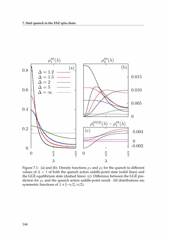
7. Néel quench in the XXZ spin chain
0
0.2
0.4
0.6
0.8
0 π4
π2
λ
ρsp1 (λ)
(a)
0
0.005
0.010
0.015
ρsp2 (λ)
(b)
0 π4
π2
-0.0020
0.004
λ
ρGGE1 (λ)− ρsp1 (λ)
(c)
∆ = 1.2∆ = 1.5∆ = 2∆ = 5∆ =∞
Figure 7.1: (a) and (b): Density functions ρ1 and ρ2 for the quench to dierentvalues of ∆ > 1 of both the quench action saddle-point state (solid lines) andthe GGE equilibrium state (dashed lines). (c): Dierence between the GGE pre-diction for ρ1 and the quench action saddle-point result. All distributions aresymmetric functions of λ ∈ [−π/2, π/2).
144

-1
− 23
− 13
0
1 3 5 7 9
∆
〈σz1σ
z2〉
0
0.02
1 2
δ〈σz1σ
z2〉
Figure 7.2: Correlator 〈σz1σ
z2〉 evaluated on the quench action steady state (solid
lines) and on the GGE (dashed lines). The energy sum rule 2〈σx1 σ
x2 〉 +∆〈σ
z1σ
z2〉
−∆ explains the exact value of −1/3 at the isotropic point ∆ 1. Numericalerrors are 10−5 or smaller. Both sets of data are in agreement with the nite-sizecomputations of Ref. [170], within the numerical precision of the latter. Inset:Relative dierence between the GGE prediction and the quench action saddle-point result, δ〈σz
1σz2〉 1 − 〈σz
1σz2〉GGE/〈σz
1σz2〉sp.

7. Néel quench in the XXZ spin chain
0
0.2
0.4
0.6
0.8
1
1 3 5 7 9
∆
〈σz1σ
z3〉
(a)
-0.09
00.02
1 2
δ〈σz1σ
z3〉
0.11
0.12
0.13
1 1.01 1.02 1.03
∆
〈σz1σ
z3〉
(b) 〈σz1σ
z3〉sp
〈σz1σ
z3〉GGE
〈σz1σ
z3〉NLCE
Figure 7.3: (a) The same as Fig. 7.2 for 〈σz1σ
z3〉. (b) Comparison between the
quench action, the GGE prediction, and the NLCE result close to the isotropicpoint. Error-bars in the NLCE data display an interval of condence that in-cludes all resummation results (except for ∆1.015) ( See supplementary mate-rials of [4]).
146
CHAPTER 8
Conclusions and Future Directions
Louis, I think this is the beginning ofa beautiful friendship.
Rick Blaine in Casablanca,M. Curtiz
Weare nally in position to spend somewords to summarize thework presentedin this thesis. We have seen in the introduction how interacting integrable sys-tems constitute prototype models from which one can understand many-bodyquantum systems in and out of equilibrium. The computation of physically rel-evant observables, like correlation functions of local operators, provides a solidplatform where one can test numerical or perturbative approaches and to ob-tain controlled predictions that can be experimentally accessed. Moreover theseare tailored models where to test generic hypothesis regarding the relaxation ofisolated quantum systems after the release from an initial pure state (quantumquench). Naively one may think that integrable models are not qualitatively dif-ferent from free models (ideal quantum gases) since they also have large sets ofconserved quantities that allow for an exact solution. However the phenomenol-ogy of integrable models is much richer, allowing us to draw more generic con-clusions on the behavior of many-body quantum systems from their behavior.
The initial studies on the non-equilibriumdynamics ofmany-body systems havebeen focusing on freemodels, ormodelswhich aremappable to free gases of par-ticles (bosons or fermions). Results on the exact post-quench steady states foran interacting many-body system (Lieb-Liniger model and the XXZ spin chain)are provided in this thesis. Besides their intrinsic relevance, they also underlinehow not only the thermal Gibbs ensemble is far from being the correct steadystate providing the late time expectation values of physical observables ans howits simple generalization for systems with more conserved quantities, the GGEensemble, is in most cases much harder to implement than for free models. Thequench from a Bose-Einstein condensate to the interacting Lieb-Liniger Bose gasdisplayed howan expansion of theGGEdensitymatrix in terms of the ultra-localcharges is hopeless in order to get the exact steady state, an analysis that led torecognize the importance of quasi-local charges for models on the continuumand for interacting eld theories [157]. The study of the out-of-equilibrium XXZspin chain brought similar conclusions. There the most striking result is thatthe presence of bound states in the theory, a clear feature of truly interacting
147
8. Conclusions and Future Directions
models, appears to be related with an extra class of quasi-local symmetry whichneeds to be taken into account in the thermodynamic description of the model.A GGE ensemble which takes care of xing only the ultra-local conserved quan-tities fails to predict the correct distribution of bound states in the steady stateafter a quench from a generic initial state with an extensive amount of energy.Therefore the test of the GGE hypothesis on an integrable, yet interacting modelas the XXZ spin chain has shed some light on various aspects of the relaxationof isolated quantum models that would have been hidden in free models.
The problem of nding a complete set of relevant conserved operators for theXXZ model, or in general for any interacting integrable lattice model, in orderto build a GGE density matrix for any initial state is one of the main open prob-lems at the moment. It is on the other hand reasonable to expect that it will besolved in the near future. Numerical studies [191] have underlined the presenceof quasi-local conserved charges, represented by families of mutually commut-ing operators that extend on the whole system, that up to now where ignoredby the community of physicist working on integrable models, where the com-mon belief has been that the logarithmic derivatives of the transfer matrix yielda complete set of local charges. This argument is based on the idea that for anynite chain, with N spins and xed magnetization 〈σz
〉 12 −
MN , a number M
of derivatives of the transfer matrix gives enough conserved operators to x anyBethe state in the spectrum. This reasoning however fails in the thermodynamiclimit, where a proper distinction between local and non-local operators can bemade and where only a restricted number of conserved quantities is relevantfrom the point of view of local observables.
The presence of quasi-local conserved charges in the XXZ model is on the otherhand a very exciting fact: it tells us that the integrability of the model is deeperthan we could expect. For example they are responsible for the nite Drudeweight of the model in its gapless regime, and on the other hand they are re-lated to exact steady states of boundary-driven spin chains [113].Moreover as shown in [91] in the presence of a weak external potential Vext to anintegrable system with Hamiltonian H, operators that are eectively conservedby the unitary time evolution e−it(H+Vext ) for long times after the quench couldexist (namely many of their matrix elements can be eectively treated as timeindependent quantities for very long times). These charges are quasi-local op-erators that can be represented as linear combinations of the local ones (whichare clearly not conserved under the perturbation Vext)
Q
∞∑a1
caQa .
We can therefore expect that if the integrable system has many quasi-local con-served quantities as Q some of its integrable properties are less likely to be bro-
148
8.0.
ken by the presence of a weak non-integrable perturbation. It will be then veryinteresting to address the mechanism of integrability breaking involving alsoquasi-local conserved quantities.
The other main point addressed in this thesis is the computation of the full post-quench time evolution, focusing in particular on the Lieb-Linigermodel. Besidespossibly oering experimentally accessible results (the time evolution for smalltimes is much more relevant from the experimental point of view which areusually limited in the range of time) it also undercovered the role of the emerg-ing thermodynamic excitations as a means to characterize both equilibrium andnon-equilibrium correlations. Indeed the quench action method gives us a toolto describe correlations of physical operators at times t 0+ after the quench byeectively decomposing the initial state as an eective dilute gas of macroscopicparticle-hole excitations on the saddle point state. The sumover such excitations,weighted by their matrix elements for any local operators (form factors), leads tothe full thermodynamic time evolution of their expectation values. In the largetimes limit t → +∞ all the excitations have dephased and only the pure saddlepoint state eectively characterizes the system. On the other hand a similar sumover the same type of excitations gives the equilibriumdynamical two-point cor-relation functions of local operators 〈O(x , t)O(0)〉 in the thermodynamic limit.In the case of low temperatures they can be treated with eective eld theorymethods which lead to a universal description of low temperature correlationfunctions in one dimensional interacting quantum systems [171]. We are thenin position to extend such universal description to the whole non-equilibriumdynamics.
Another interesting problem is to specify the role of the initial state in determin-ing the whole time evolution without focusing only on the innite time limit.It turns out that only the leading part of the overlap coecients is responsiblefor the full time evolution after a quench. This underlines how the thermody-namic limit of the overlaps, aswell as thematrix elements, constitutes an optimalcoarse graining analysis of the microscopic model which allows to isolate therelevant data that one can use to reconstruct the whole physically relevant infor-mation on the system. The matrix elements of local operators are well-knownfor any nite size system from the algebraic Bethe ansatz and one has then totake the thermodynamic limit of their complicated expressions. This processis quite involved and in this thesis a rst step in this direction was made. Onthe other hand, at the moment there are no generic explicit expressions for theoverlaps of Bethe state related to dierent scattering matrices, except for the fewcases that are treated in this thesis. Therefore the computation of the overlapsin the Lieb-Liniger model between Bethe state with dierent coupling constantsc or between two dierent XXZ eigenstates with two dierent anisotropies ∆remains an open problem. On the other hand it seems feasible to imagine thattheir thermodynamically relevant parts can be extracted by taking a zero-density
149

8. Conclusions and Future Directions
thermodynamic limit which does not require the full knowledge of their exactexpressions valid at any nite size. This would be an exciting and promisingdirection to take in the future, together with the search for a method to gener-alize the algebraic Bethe ansatz with a "super-algebra" connecting theories withdierent scattering matrices. The rst step would be to determine the overlapbetween a Bethe state and a generic spin state in the XXZ model or equivalentlythe overlap of the Lieb-Liniger states with all the eigenstates of the free bosonictheory. Such objects would form a basis to determine any other overlap.Finally the time evolution in a lattice model as the XXZ spin chain is denitelya problem to address in the future. Here the relevant macroscopic excitationsare not only particle-hole excitations but also recombinations between boundstates. This clearly makes the problem of determining the whole time evolutioncomputationally more dicult, even if the general approach remains the sameas in the Lieb-Liniger model.
150


Bibliography
[1] J. De Nardis, B. Wouters, M. Brockmann, and J.-S. Caux. Solution for aninteraction quench in the Lieb-Liniger Bose gas. Phys. Rev. A, 89:033601,2014.
[2] M. Brockmann, J. De Nardis, B. Wouters, and J.-S. Caux. A Gaudin-likedeterminant for overlaps of Néel and XXZ Bethe states. J. Phys. A: Math.Theor., 47:145003, 2014.
[3] M. Brockmann, J. De Nardis, B. Wouters, and J.-S. Caux. Néel-XXZ stateoverlaps: odd particle numbers and Lieb–Liniger scaling limit. J. Phys. A:Math. Theor., 47:345003, 2014.
[4] B. Wouters, J. De Nardis, M. Brockmann, D. Fioretto, M. Rigol, and J.-S. Caux. Quenching the Anisotropic Heisenberg Chain: Exact Solutionand Generalized Gibbs Ensemble Predictions. Phys. Rev. Lett., 113:117202,2014.
[5] M. Brockmann, B. Wouters, D. Fioretto, J. De Nardis, R. Vlijm, and J.-S.Caux. Quench action approach for releasing the Néel state into the spin-1/2 XXZ chain. J. Stat. Mech.: Th. Exp., 2014(12):P12009, 2014.
[6] J. De Nardis and J.-S. Caux. Analytical expression for a post-quench timeevolution of the one-body density matrix of one-dimensional hard-corebosons. J. Stat. Mech. Theor. Exp., 2014(12):P12012, 2014.
[7] J. De Nardis and M. Panl. Density form factors of the 1D Bose gas fornite entropy states. J. Stat. Mech. Theor. Exp., 2015(2):P02019, 2015.
[8] J. De Nardis, L. Piroli, and J.-S. Caux. Relaxation dynamics of local ob-servables in integrable systems. arXiv:1505.03080.
[9] M. Panl, J. DeNardis, and J.-S. Caux. Metastable Criticality and the SuperTonks-Girardeau Gas. Phys. Rev. Lett., 110:125302, Mar 2013.
[10] F. Bacon. Novum Organum Scientiarum. London, 1620.
[11] R. Descartes. Discours de la méthode pour bien conduire sa raison, et chercherla vérité dans les sciences. Leiden, 1637.
[12] E. Ising. Beitrag zur Theorie des Ferromagnetismus. Zeitschrift für Physik,31:253–258, 1925.
[13] N. D. Mermin and H. Wagner. Absence of Ferromagnetism or Antifer-romagnetism in One- or Two-Dimensional Isotropic Heisenberg Models.Phys. Rev. Lett., 17:1133–1136, Nov 1966.
153
[14] L. Onsager. Crystal Statistics. I. A Two-DimensionalModel with anOrder-Disorder Transition. Phys. Rev., 65:117–149, 1944.
[15] A. Brunello, F. Dalfovo, L. Pitaevskii, S. Stringari, and F. Zambelli. Mo-mentum transferred to a trapped bose-einstein condensate by stimulatedlight scattering. Phys. Rev. A, 64:063614, Nov 2001.
[16] J.-S. Caux. Correlation functions of integrable models: A description ofthe ABACUS algorithm. J. Math. Phys., 50(9):095214, September 2009.
[17] F. D. M. Haldane. ‘Luttinger liquid theory’ of one-dimensional quantumuids. I. Properties of the Luttinger model and their extension to the gen-eral 1D interacting spinless Fermi gas. J. Phys C: Sol. St. Phys., 14(19):2585,1981.
[18] F. D. M. Haldane. "Demonstration of the ‘Luttinger liquid’ character ofBethe-ansatz-soluble models of 1-D quantum uids". Phys. Lett. A, 81(2-3):153 – 155, 1981.
[19] F. D. M. Haldane. Eective Harmonic-Fluid Approach to Low-EnergyProperties of One-Dimensional Quantum Fluids. Phys. Rev. Lett.,47(25):1840–1843, 1981.
[20] T. Giamarchi. Quantum Physics in One Dimension. OxfordUniversity Press,Oxford, 2004.
[21] M. A. Cazalilla. Bosonizing one-dimensional cold atomic gases. J. Phys. B:AMOP, 37(7):S1, 2004.
[22] E. H. Lieb and W. Liniger. Exact Analysis of an Interacting Bose Gas. I.The General Solution and the Ground State. Phys. Rev., 130(4):1605–1616,1963.
[23] E. H. Lieb. Exact Analysis of an Interacting Bose Gas. II. The ExcitationSpectrum. Phys. Rev., 130:1616–1624, May 1963.
[24] N. M. Bogoliubov and V. E. Korepin. "Correlation length of the one-dimensional Bose gas". Nucl. Phys. B, 257:766 – 778, 1985.
[25] A. Brunello, F. Dalfovo, L. Pitaevskii, S. Stringari, and F. Zambelli. Mo-mentum transferred to a trapped Bose-Einstein condensate by stimulatedlight scattering. Phys. Rev. A, 64:063614, 2001.
[26] A. H. van Amerongen, J. J. P. van Es, P. Wicke, K. V. Kheruntsyan, andN. J. van Druten. Yang-Yang Thermodynamics on an Atom Chip. Phys.Rev. Lett., 100(9):090402, 2008.
[27] T. Kinoshita, T. Wenger, and D. S. Weiss. Observation of a One-Dimensional Tonks-Girardeau Gas. Science, 305(5687):1125–1128, 2004.
[28] T. Kinoshita, T. Wenger, and D. S. Weiss. Local Pair Correlations in One-Dimensional Bose Gases. Phys. Rev. Lett., 95(19):190406, 2005.
[29] A. Furrer, J. Mesot, and T. Strässle. Neutron Scattering in Condensed MatterPhysics. World Scientic, 2009.
[30] M. Mourigal, M. Enderle, A. Klöpperpieper, J.-S. Caux, A. Stunault, andH. M. Ronnow. Fractional spinon excitations in the quantum Heisenbergantiferromagnetic chain. Nat. Phys., 9(7):435 – 441, 2013.
[31] B. Lake, D. A. Tennant, J.-S. Caux, T. Barthel, U. Schollwöck, S. E. Nagler,and C. D. Frost. Multispinon Continua at Zero and Finite Temperature ina Near-Ideal Heisenberg Chain. Phys. Rev. Lett., 111:137205, 2013.
[32] J. Schlappa, K. Wohlfeld, K. J. Zhou, M. Mourigal, M. W. Haverkort, V. N.Strocov, L. Hozoi, C. Monneyand S. Nishimoto, S. Singh, A. Revcolevschi,J.-S. Caux, L. Patthey, H.M.Ronnow, J. vandenBrink, andT. Schmitt. Spin-orbital separation in the quasi-one-dimensional Mott insulator Sr2CuO3.Nature, 485:82–86, 2012.
[33] M. Panl, J. DeNardis, and J.-S. Caux. Metastable Criticality and the SuperTonks-Girardeau Gas. Phys. Rev. Lett., 110:125302, 2013.
[34] P. Calabrese and J. Cardy. Time Dependence of Correlation Functions Fol-lowing a Quantum Quench. Phys. Rev. Lett., 96:136801, 2006.
[35] M. Rigol, V. Dunjko, V. Yurovsky, and M. Olshanii. Relaxation in a Com-pletely IntegrableMany-BodyQuantumSystem: AnAb Initio Study of theDynamics of the Highly Excited States of 1D Lattice Hard-Core Bosons.Phys. Rev. Lett., 98:050405, 2007.
[36] A. Polkovnikov, K. Sengupta, A. Silva, and M. Vengalattore. Colloquium:Nonequilibrium dynamics of closed interacting quantum systems. Rev.Mod. Phys., 83:863, 2011.
[37] T. Kinoshita, T. Wenger, and D. S. Weiss. A quantum Newton’s cradle.Nature, 440:900, 2006.
[38] E. Haller, M. Gustavsson, M. Manfred, J. G. Danzl, R. Hart, G. Pupillo, ,and H.-C. Naegerl. Realization of an Excited, Strongly Correlated Quan-tum Gas Phase. Science, 325(5945):1224–1227, 2009.
[39] M. Gring, M. Kuhnert, T. Langen, T. Kitagawa, B. Rauer, M. Schreitl,I. Mazets, D. Adu Smith, E. Demler, and J. Schmiedmayer. Relaxationand Prethermalization in an Isolated Quantum System. Science, 337:1318,2012.

[40] M. Cheneau, P. Barmettler, D. Poletti, M. Endres, P. Schauss, T. Fukuhara,C. Gross, I. Bloch, C. Kollath, and S. Kuhr. Light-cone-like spreading ofcorrelations in a quantum many-body system. Nature, 481:484, 2012.
[41] T. Langen, R. Geiger, M. Kuhnert, B. Rauer, and J. Schmiedmayer. Lo-cal emergence of thermal correlations in an isolated quantummany-bodysystem. Nature Physics, 9:640–643, 2013.
[42] I. Meinert, M. Mark, E. Kirilov, K. Lauber, P. Weinmann, M. Gröbner,A. Daley, and H.-C. Nägerl. Observation of many-body dynamics in long-range tunneling after a quantum quench. Science, 344(6189):1259–1262,2014.
[43] F. Meinert, M. J. Mark, E. Kirilov, K. Lauber, P. Weinmann, A. J. Daley,and H.-C. Nägerl. QuantumQuench in an Atomic One-Dimensional IsingChain. Phys. Rev. Lett., 111:053003, Jul 2013.
[44] S. Trotzky, Y-A. Chen, A. Flesch, I. P. McCulloch, U. Schollwöck, J. Eisert,and I. Bloch. Probing the relaxation towards equilibrium in an isolatedstrongly correlated one-dimensional Bose gas. Nat. Phys., 8:325, 2012.
[45] T. Langen, S. Erne, Geiger R., Rauer B., Schweigler T., Kuhnert M.,Rohringer W., I.E. Mazets, Gasenzer T., and Schmiedmayer J. Experimen-tal observation of a generalized Gibbs ensemble. Science, 348(6231):207–211, 2015.
[46] T.W.B. Kibble. Some implications of a cosmological phase transition. Phys.Rep., 67(1):183 – 199, 1980.
[47] W. Zurek. Cosmological experiments in superuid helium? Nature,317:505, 1985.
[48] G. D. Moore and D. Teaney. How much do heavy quarks thermalize in aheavy ion collision? Phys. Rev. C, 71:064904, 2005.
[49] J. von Neumann. Beweis des Ergodensatzen und des H-Theorems in derneuen Mechanik. Zietschrift für Physik, 57:30–70, 1929.
[50] S. Goldstein, J. L. Lebowitz, R. Tumulka, and N. Zanghì. Long-time be-havior of macroscopic quantum systems. Eur. Phys. J. H, 35(2):173–200,2010.
[51] Eugene P. W. Characteristic vectors of bordered matrices with innite di-mensions. Ann. Math., 62(3):548–564, 1955.
[52] J. M. Deutsch. Quantum statistical mechanics in a closed system. Phys.Rev. A, 43:2046–2049, Feb 1991.
[53] M. Srednicki. The approach to thermal equilibrium in quantized chaoticsystems. J Phys A. Math. Theor., 32(7):1163, 1999.
[54] M. Rigol. Breakdown of Thermalization in Finite One-Dimensional Sys-tems. Phys. Rev. Lett., 103:100403, Sep 2009.
[55] G. Biroli, C. Kollath, and A. M. Läuchli. Eect of Rare Fluctuations on theThermalization of Isolated Quantum Systems. Phys. Rev. Lett., 105:250401,Dec 2010.
[56] M. Rigol and M. Srednicki. Alternatives to Eigenstate Thermalization.Phys. Rev. Lett., 108:110601, Mar 2012.
[57] W. Beugeling, R. Moessner, and Masudul Haque. Finite-size scaling ofeigenstate thermalization. Phys. Rev. E, 89:042112, Apr 2014.
[58] V. Alba. Eigenstate thermalization hypothesis and integrability in quan-tum spin chains. Phys. Rev. B, 91:155123, Apr 2015.
[59] N. J. Zabusky andM.D.Kruskal. Interaction of "Solitons" in aCollisionlessPlasma and the Recurrence of Initial States. Phys. Rev. Lett., 15:240–243,Aug 1965.
[60] V. Arnold, A. Weinstein, and K. Vogtmann. Mathematical Methods of Clas-sical Mechanics. Springer, 1997.
[61] M. Rigol, V. Dunjko, and M. Olshanii. Thermalization and its mechanismfor generic isolated quantum systems. Nature, 452:854–858, 2008.
[62] P. Barmettler, M. Punk, V. Gritsev, E. Demler, and E. Altman. Relax-ation of Antiferromagnetic Order in Spin-1/2 Chains Following a Quan-tum Quench. Phys. Rev. Lett., 102:130603, 2009.
[63] P. Calabrese, F. H. L. Essler, and M. Fagotti. Quantum Quench in theTransverse-Field Ising Chain. Phys. Rev. Lett., 106:227203, 2011.
[64] P. Calabrese, F. H. L. Essler, andM. Fagotti. Quantum quench in the trans-verse eld Ising chain: I. Time evolution of order parameter correlators. J.Stat. Mech.: Th. Exp., 2012:P07016, 2012.
[65] J. Mossel and J.-S. Caux. Exact time evolution of space- and time-dependent correlation functions after an interaction quench in the one-dimensional Bose gas. New J. Phys., 14(7):075006, 2012.
[66] M. Fagotti and F. H. L. Essler. Stationary behaviour of observables after aquantum quench in the spin-1/2 Heisenberg XXZ chain. J. Stat. Mech.: Th.Exp., page P07012, 2013.

[67] M. Fagotti and F. H. L. Essler. Reduced density matrix after a quantumquench. Phys. Rev. B, 87:245107, Jun 2013.
[68] M. Collura, S. Sotiriadis, and P. Calabrese. Equilibration of a Tonks-Girardeau Gas Following a Trap Release. Phys. Rev. Lett., 110:245301, Jun2013.
[69] Analytic results for a quantum quench from free to hard-core one-dimensional bosons.
[70] L. Bucciantini, M. Kormos, and P. Calabrese. Quantum quenches fromexcited states in the Ising chain. J. Phys. A: Math. Theor., 47:175002, 2014.
[71] M.A. Cazalilla. Eect of Suddenly Turning on Interactions in the LuttingerModel. Phys. Rev. Lett., 97:156403, 2006.
[72] A. Iucci and M. A. Cazalilla. Quantum quench dynamics of the Luttingermodel. Phys. Rev. A, 80:063619, 2009.
[73] S. Sotiriadis and P. Calabrese. Validity of the GGE for quantum quenchesfrom interacting to noninteracting models. J. Stat. Mech.: Th. Exp., pageP07024, 2014.
[74] J.-S. Caux and R.M. Konik. Constructing the Generalized Gibbs Ensembleafter a Quantum Quench. Phys. Rev. Lett., 109:175301, 2012.
[75] B. Pozsgay. J. Stat. Mech.: Th. Exp., page P10045, 2014.
[76] B. Pozsgay. The generalized Gibbs ensemble for Heisenberg spin chains.J. Stat. Mech.: Th. Exp., page P07003, 2013.
[77] M. Fagotti. On conservation laws, relaxation and pre-relaxation after aquantum quench. J. Stat. Mech. Theor. Exp., 2014(3):P03016, 2014.
[78] B. Pozsgay, M. Mestyán, M. A. Werner, M. Kormos, G. Zaránd, andG. Takács. Correlations after QuantumQuenches in the XXZ Spin Chain:Failure of the Generalized Gibbs Ensemble. Phys. Rev. Lett., 113:117203,2014.
[79] "J.-S." Caux and F. H. L. Essler. Time Evolution of Local Observables AfterQuenching to an Integrable Model. Phys. Rev. Lett., 110:257203, 2013.
[80] L. Bonnes, F. H. L. Essler, and A. M. Läuchli. “Light-Cone” DynamicsAfter Quantum Quenches in Spin Chains. Phys. Rev. Lett., 113:187203, Oct2014.
[81] B. Bertini, D. Schuricht, and F. H. L. Essler. Quantum quench in the sine-Gordon model. J. Stat. Mech.: Th. Exp., page P10035, 2014.

[82] A. De Luca, G. Martelloni, and J. Viti. Stationary states in a free fermionicchain from the quench action method. Phys. Rev. A, 91:021603, Feb 2015.
[83] E. Bettelheim. Towards a non-equilibrium bethe ansatz for the kondomodel. J. Phys. A: Math. Theor., 48(16):165003, 2015.
[84] E. H. Lieb and D. W. Robinson. The nite group velocity of quantum spinsystems. Commun. Math. Phys., 28(3):251–257, 1972.
[85] C. Gogolin, M. P. Müller, and J. Eisert. Absence of Thermalization in Non-integrable Systems. Phys. Rev. Lett., 106:040401, Jan 2011.
[86] J.Mossel and J.-S. Caux. Relaxation dynamics in the gapped XXZ spin-1/2chain. New J. Phys., 12:055028, 2010.
[87] F. H. L. Essler, S. Kehrein, S. R. Manmana, and N. J. Robinson. Quenchdynamics in a model with tuneable integrability breaking. Phys. Rev. B,89:165104, Apr 2014.
[88] B. Bertini and M. Fagotti. Pre-relaxation in weakly interacting models.arXiv:1501.07260, 2015.
[89] M. Moeckel and S. Kehrein. Interaction Quench in the Hubbard Model.Phys. Rev. Lett., 100:175702, May 2008.
[90] M. Marcuzzi, J. Marino, A. Gambassi, and A. Silva. Prethermalization ina Nonintegrable Quantum Spin Chain after a Quench. Phys. Rev. Lett.,111:197203, Nov 2013.
[91] G. Brandino, J.-S. Caux, and R. Konik. Relaxation dynamics of con-served quantities in a weakly non-integrable one-dimensional Bose gas.arXiv:1301.0308.
[92] W. Beugeling, R. Moessner, and M. Haque. O-diagonal matrix elementsof local operators inmany-body quantum systems. Phys. Rev. E, 91:012144,Jan 2015.
[93] N. P. Konstantinidis. Thermalization away from integrability and the roleof operator o-diagonal elements. Phys. Rev. E, 91:052111, May 2015.
[94] T. Kitagawa, A. Imambekov, J Schmiedmayer, and E. Demler. The dynam-ics and prethermalization of one-dimensional quantum systems probedthrough the full distributions of quantumnoise. New J. Phys., 13(7):073018,2011.
[95] T. Langen, M. Gring, M. Kuhnert, B. Rauer, R. Geiger, D. Smith, I. Mazets,and J. Schmiedmayer. Prethermalization in one-dimensional Bose gases:Description by a stochastic Ornstein-Uhlenbeck process. Eur. Phys. J.,217(1):43–53, 2013.
[96] T. Prosen. Time Evolution of a Quantum Many-Body System: Transitionfrom Integrability to Ergodicity in the Thermodynamic Limit. Phys. Rev.Lett., 80:1808–1811, Mar 1998.
[97] T. Prosen. Ergodic properties of a generic nonintegrable quantum many-body system in the thermodynamic limit. Phys. Rev. E, 60:3949–3968, Oct1999.
[98] W. Heisenberg. Zur Theorie des Ferromagnetismus. Z. Phys., 49:619, 1928.
[99] H. Bethe. Zur Theorie derMetalle. I. Eigenwerte und Eigenfunktionen derlinearen Atomkette. Z. Phys., 71:205, 1931.
[100] R. Orbach. Linear Antiferromagnetic Chain with Anisotropic Coupling.Phys. Rev., 112:309, 1958.
[101] J.-S. Caux and J. Mossel. Remarks on the notion of quantum integrability.J. Stat. Mech.: Th. Exp., 2011(02):P02023, 2011.
[102] J. Mossel. Quantum integrable models out of equilibrium. PhD thesis - Uni-versity of Amsterdam, 2012.
[103] M. Panl. Density uctuations in the 1D Bose Gas. PhD thesis - Universityof Amsterdam, 2013.
[104] B. Sutherland. Nondiractive scattering: Scattering from kaleidoscopes.J. Math. Phys., 21(7):1770–1775, 1980.
[105] B. Sutherland. Beautiful Models. World Scientic, 2004.
[106] V. E. Korepin, N. M. Bogoliubov, and A. G. Izergin. Quantum InverseScattering Method and Correlation Functions. Cambridge Univ. Press, Cam-bridge, 1993.
[107] M. Gaudin. La fonction d’onde de Bethe. Masson, Paris, 1983. ; Englishtranslation by J.-S. Caux 2014 (Cambridge: Cambridge University Press).
[108] F. Franchini. Notes on Bethe Ansatz Techniques. SISSA, Trieste, 2011.
[109] P. Mazur. "Non-ergodicity of phase functions in certain systems". Physica,43(4):533 – 545, 1969.
[110] M. Sirugue and A. Verbeure. On the lower bound of Mazur for autocorre-lation functions. Ergodicity. Physica, 65(1):181 – 186, 1973.
[111] M. Suzuki. "Ergodicity, constants of motion, and bounds for susceptibili-ties". Physica, 51(2):277 – 291, 1971.
[112] T. Prosen and E. Ilievski. Families of Quasilocal Conservation Laws andQuantum Spin Transport. Phys. Rev. Lett., 111:057203, 2013.
[113] T. Prosen. Quasilocal conservation laws in XXZ spin-1/2 chains: open,periodic and twisted boundary conditions. Nucl. Phys. B, 886:1177, 2014.
[114] R. G. Pereira, V. Pasquier, J. Sirker, and I. Aeck. Exactly conservedquasilocal operators for the XXZ spin chain. J. Stat. Mech.: Th. Exp., pageP09037, 2014.
[115] M.Olshanii. Atomic Scattering in the Presence of an External Connementand a Gas of Impenetrable Bosons. Phys. Rev. Lett., 81:938–941, Aug 1998.
[116] R. Seiringer and J. Yin. The Lieb-LinigerModel as a Limit of Dilute Bosonsin Three Dimensions. Commun. Math. Phys., 284(2):459–479, 2008.
[117] L. Tonks. The Complete Equation of State of One, Two and Three-Dimensional Gases of Hard Elastic Spheres. Phys. Rev., 50(10):955–963,1936.
[118] C. N. Yang and C. P. Yang. Thermodynamics of a One-Dimensional Sys-tem of Bosons with Repulsive Delta-Function Interaction. J. Math. Phys.,10(7):1115–1122, 1969.
[119] F. Göhmann and V. E. Korepin. Solution of the quantum inverse problem.J. Phys. A: Math. Theor., 33(6):1199–1220, 2000.
[120] N. Kitanine, J. M. Maillet, and V. Terras. "Form factors of the XXZ Heisen-berg nite chain". Nucl. Phys. B, 554(3):647 – 678, 1999.
[121] N. A. Slavnov. Calculation of scalar products of wave functions and formfactors in the framework of the algebraic Bethe Ansatz. Theor. Math. Phys.,79:502, 1989.
[122] M. Gaudin, B. M.McCoy, and T. T.Wu. Normalization sum for the Bethe’shypothesis wave functions of the Heisenberg-Ising chain. Phys. Rev. D,23:417, 1981.
[123] V. E. Korepin. Calculation of norms of Bethe wave functions. Commun.Math. Phys., 86:391, 1982.
[124] A. Klümper. Integrability of quantum chains: Theory and applicationsto the spin-1/2 XXZ chain. In Ulrich Schollwöck, Johannes Richter, Dami-anJ.J. Farnell, and RaymodF. Bishop, editors,QuantumMagnetism, volume645 of Lecture Notes in Physics, pages 349–379. Springer Berlin Heidelberg,2004.
[125] P. Le Doussal and P. Calabrese. The KPZ equation with at initial condi-tion and the directed polymer with one free end. J. Stat. Mech. Theor. Exp.,2012(06):P06001, 2012.

[126] V. Gritsev, T. Rostunov, and E. Demler. Exactmethods in the analysis of thenon-equilibrium dynamics of integrable models: application to the studyof correlation functions for non-equilibrium 1D Bose gas. J. Stat. Mech.:Th. Exp., 2010(05):P05012, 2010.
[127] M. Brockmann. Overlaps of q-raised Néel states with XXZ Bethe statesand their relation to the Lieb-Liniger Bose gas. J. Stat. Mech.: Th. Exp.,page P05006, 2014.
[128] M. Kardar, G. Parisi, and Y.-C. Zhang. Dynamic Scaling of Growing Inter-faces. Phys. Rev. Lett., 56:889–892, Mar 1986.
[129] M. Mehta. Random Matrices. Elsevier, 2004.
[130] K. A. Takeuchi, M. Sano, T. Sasamoto, and H. Spohn. Sci. Rep. (Nature),1:34, 2011.
[131] P. Calabrese and J.-S. Caux. Correlation Functions of theOne-DimensionalAttractive Bose Gas. Phys. Rev. Lett., 98(15):150403, Apr 2007.
[132] P. Calabrese and J.-S. Caux. Dynamics of the attractive 1DBose gas: analyt-ical treatment from integrability. J. Stat. Mech.: Th. Exp., 2007(08):P08032,2007.
[133] P. Calabrese and P. LeDoussal. Exact Solution for the Kardar-Parisi-ZhangEquationwith Flat Initial Conditions. Phys. Rev. Lett., 106:250603, Jun 2011.
[134] P. Calabrese andP. LeDoussal. Interaction quench in a Lieb–Linigermodeland the KPZ equation with at initial conditions. J. Stat. Mech. Theor. Exp.,2014(5):P05004, 2014.
[135] P. Calabrese, P. Le Doussal, and A. Rosso. Free-energy distribution of thedirected polymer at high temperature. EPL, 90(2):20002, 2010.
[136] J.Mossel and J.-S. Caux. Relaxation dynamics in the gapped XXZ spin-1/2chain. New J. Phys., 12(5):055028, 2010.
[137] O. Tsuchiya. Determinant formula for the six-vertexmodel with reectingend. J. Math. Phys., 39:5946, 1998.
[138] L. Piroli and P. Calabrese. Recursive formulas for the overlaps betweenBethe states and product states in XXZHeisenberg chains. J. Phys. A:Math.Theor., 47:385003, 2014.
[139] K. K. Kozlowski and B. Pozsgay. Surface free energy of the open XXZspin-1/2 chain. J. Stat. Mech.: Th. Exp., 2012(05):P05021, 2012.
[140] B. Pozsgay. Overlaps between eigenstates of the XXZ spin-1/2 chain anda class of simple product states. J. Stat. Mech.: Th. Exp., page P06011, 2014.

[141] K. K. Kozlowski and B. Pozsgay. Surface free energy of the open XXZspin-1/2 chain. J. Stat. Mech. Theor. Exp., 2012(05):P05021, 2012.
[142] J.-S. Caux and J. M. Maillet. Computation of Dynamical CorrelationFunctions of Heisenberg Chains in a Magnetic Field. Phys. Rev. Lett.,95(7):077201, 2005.
[143] J.-S. Caux and P. Calabrese. Dynamical density-density correlations in theone-dimensional Bose gas. Phys. Rev. A, 74(3):031605, Sep 2006.
[144] M. Panl and J.-S. Caux. Finite-temperature correlations in the Lieb-Liniger one-dimensional Bose gas. Phys. Rev. A, 89:033605, Mar 2014.
[145] N. Kitanine, K. K. Kozlowski, J. M. Maillet, N. A. Slavnov, and V. Terras.Form factor approach to dynamical correlation functions in critical mod-els. J. Stat. Mech. Theor. Exp., 2012(09):P09001, 2012.
[146] N. Kitanine, K. K. Kozlowski, J. M. Maillet, N. A. Slavnov, and V. Terras. Aform factor approach to the asymptotic behavior of correlation functionsin critical models. J. Stat. Mech. Theor. Exp., 2011(12):P12010, 2011.
[147] A. Shashi, L. I. Glazman, J.-S. Caux, and A. Imambekov. Nonuniversalprefactors in the correlation functions of one-dimensional quantum liq-uids. Phys. Rev. B, 84(4):045408, 2011.
[148] K. K. Kozlowski and V. Terras. Long-time and large-distance asymptoticbehavior of the current–current correlators in the non-linear Schrödingermodel. J. Stat. Mech. Theor. Exp., 2011(09):P09013, 2011.
[149] N. A. Slavnov. Nonequal-time current correlation function in a one-dimensional Bose gas. Theor. Math. Phys., 82:273, 1990.
[150] A. Shashi, M. Panl, J.-S. Caux, and A. Imambekov. Exact prefactors instatic and dynamic correlation functions of one-dimensional quantum in-tegrable models: Applications to the Calogero-Sutherland, Lieb-Liniger,and XXZ models. Phys. Rev. B, 85:155136, 2012.
[151] V. E. Korepin and N. A. Slavnov. Time dependance of the denisty-densitytemperature correlation function of a one-dimensional bose gas. Nucl.Phys. B, 340:757–766, 1990.
[152] B Pozsgay and G Takács. Form factor expansion for thermal correlators. J.Stat. Mech. Theor. Exp., 2010(11):P11012, 2010.
[153] J. Brand and A. Yu. Cherny. Dynamic structure factor of the one-dimensional Bose gas near the Tonks-Girardeau limit. Phys. Rev. A,72:033619, 2005.
[154] L. P. Pitaevskii and E. M. Lifshitz. Statistical Physics, Part 2. Vol. 9 .Butterworth-Heinemann, 1980.
[155] B. Davies. Higher conservation laws for the quantum non-linearSchrödinger equation. Physica A, 167(2):433 – 456, 1990.
[156] M. Kormos, A. Shashi, Y.-Z. Chou, J.-S. Caux, and A. Imambekov. Inter-action quenches in the one-dimensional Bose gas. Phys. Rev. B, 88:205131,2013.
[157] F. H. L. Essler, G. Mussardo, and M. Panl. Generalized Gibbs ensemblesfor quantum eld theories. Phys. Rev. A, 91:051602, May 2015.
[158] F. Bornemann. On the Numerical Evaluation of Fredholm Determinants.Math. Comp., 79:871–915, 2010.
[159] M. Kormos, Y.-Z. Chou, and A. Imambekov. Exact Three-Body Local Cor-relations for Excited States of the 1D Bose Gas. Phys. Rev. Lett., 107:230405,Dec 2011.
[160] B. Pozsgay. Mean values of local operators in highly excited Bethe states.J. Stat. Mech.: Th. Exp., 2011(01):P01011, 2011.
[161] I. Carusotto, R. Balbinot, A. Fabbri, andA. Recati. Density correlations andanalog dynamical Casimir emission of Bogoliubov phonons inmodulatedatomic Bose-Einstein condensates. Eur. Phys. J. D, 56(3):391–404, 2010.
[162] A. Gil, J. Segura, and N. M. Temme. "Computation of the modied Besselfunction of the third kind of imaginary orders: uniform Airy-type asymp-totic expansion ". JCAM, 153(1–2):225 – 234, 2003. Proceedings of the 6thInternational Symposium on Orthogonal Poly nomials, Special Functionsand their Applications, Rome, Italy, 18-22 June 2001.
[163] D. Fioretto and G. Mussardo. Quantum quenches in integrable eld the-ories. New J. Phys., 12:055015, 2010.
[164] J. Mossel and J.-S. Caux. Exact time evolution of space- and time-dependent correlation functions after an interaction quench in the one-dimensional Bose gas. New J Phys, 14(7):075006, 2012.
[165] C. Karrasch, J. Rentrop, D. Schuricht, and V. Meden. Luttinger-liquid uni-versality in the time evolution after an interaction quench. Phys. Rev. Lett.,109:126406, 2012.
[166] A. Faribault and D. Schuricht. Integrability-Based Analysis of theHyperne-Interaction-Induced Decoherence in QuantumDots. Phys. Rev.Lett., 110:040405, Jan 2013.

[167] G.Mussardo. Innite-TimeAverage of Local Fields in an Integrable Quan-tum Field Theory After a Quantum Quench. Phys. Rev. Lett., 111:100401,2013.
[168] M. Kormos, M. Collura, and P. Calabrese. Analytic results for a quan-tum quench from free to hard-core one-dimensional bosons. Phys. Rev. A,89:013609, 2014.
[169] D. Fioretto, J.-S. Caux, and V. Gritsev. Exact out-of-equilibrium centralspin dynamics from integrability. New J. Phys., 16(4):043024, 2014.
[170] M. Fagotti, M. Collura, F. H. L. Essler, and P. Calabrese. Relaxation afterquantum quenches in the spin-1/2 Heisenberg XXZ chain. Phys. Rev. B,89:125101, 2014.
[171] A. Imambekov and L. I. Glazman. Universal Theory of Nonlinear Lut-tinger Liquids. Science, 323(5911):228–231, 2009.
[172] A. Imambekov and L. I. Glazman. Phenomenology of One-DimensionalQuantum Liquids Beyond the Low-Energy Limit. Phys. Rev. Lett.,102:126405, Mar 2009.
[173] C. Karrasch, R. G. Pereira, and J. Sirker. Low temperature dynamics ofnonlinear Luttinger liquids. arXiv:1410.2226, 2014.
[174] M. Takahashi. Thermodynamics of one-dimensional solvable models. Cam-bridge University Press, Cambridge, 1999.
[175] D. M. Gangardt and G. V. Shlyapnikov. Stability and Phase Coherence ofTrapped 1D Bose Gases. Phys. Rev. Lett., 90:010401, Jan 2003.
[176] B. Pozsgay. Local correlations in the 1D Bose gas from a scaling limit ofthe XXZ chain. J. Stat. Mech. Theor. Exp., 2011(11):P11017, 2011.
[177] L. Piroli and P Calabrese. arXiv:1506.06539, 2015.
[178] S. Sotiriadis and P. Calabrese. Validity of the GGE for quantum quenchesfrom interacting to noninteracting models. J. Stat. Mech.: Th. Exp.,2014(7):P07024, 2014.
[179] M. Girardeau. Relationship between Systems of Impenetrable Bosons andFermions in One Dimension. J. Math. Phys., 1(6):516–523, 1960.
[180] M. Zvonarev. Correlations in 1d boson and fermion systems: exact results. PhDthesis - Copenhagen University, 2005.
[181] A. Lenard. Momentum Distribution in the Ground State of the One-Dimensional System of Impenetrable Bosons. J. Math. Phys., 5(7):930–943,1964.

[182] A. M. Tsvelik and P. B. Wiegmann. Exact results in the theory of magneticalloys. Adv. Phys., 32:453, 1983.
[183] M. Takahashi. One-DimensionalHeisenbergModel at Finite Temperature.Prog. Theor. Phys., 46:401, 1971.
[184] M. Takahashi and M. Suzuki. One-Dimensional Anisotropic HeisenbergModel at Finite Temperatures. Prog. Theor. Phys., 48:2187, 1972.
[185] R. P. Feynman. Forces in molecules. Phys. Rev., 56:340, 1939.
[186] J.-S. Caux, R.Hagemans, and J.M.Maillet. Computation of dynamical cor-relation functions of Heisenberg chains: the gapless anisotropic regime. J.Stat. Mech.: Th. Exp., page P09003, 2005.
[187] M. Mestyán and B. Pozsgay. Short distance correlators in the XXZspin chain for arbitrary string distributions. J. Stat. Mech. Theor. Exp.,2014(9):P09020, 2014.
[188] C. Trippe, F. Göhmann, and A. Klümper. Short-distance thermal correla-tions in the massive XXZ chain. Eur. Phys. J. B, 73(2):253–264, 2010.
[189] M. Takahashi, M. Shiroishi, and A. Klümper. Equivalence of TBA andQTM. J. Phys. A Math. Theor., 34(13):L187, 2001.
[190] B. Pozsgay. Failure of the Generalized Eigenstate Thermalization Hypoth-esis in integrable models with multiple particle species. arXiv:1406.4613.
[191] M. Mierzejewski, P. Prelovšek, and T. Prosen. Identifying Local andQuasilocal Conserved Quantities in Integrable Systems. Phys. Rev. Lett.,114:140601, Apr 2015.
Summary
Since the birth of the scientic method it became widespread in the physical sci-ences the idea that natural phenomena can always be understood by studyingthe physics of each of their elementary constituents. While this attitude led toimmense discoveries on the sub-atomic particles that brought to a unied the-ory of electromagnetism, weak and strong interactions inside the nuclei (the socalled standard model), on the other hand it left many big questions with noproper answer. For example, one of the most fascinating concepts of modern-day physics is emergence, the process whereby complex macroscopic propertiesarise from the interaction of many simple-behaved constituents. For example,when interactions among the single constituents of a system becomes large, theproperties of the whole are in general completely dierent from the propertiesof the single element. New undiscovered physics therefore emerges from thepresence of such non-trivial interactions which cannot usually be treated per-turbatevely, namely they cannot be addressed assuming that the interactionsare small. When the constituents are conned to a one-dimensional geometryfor example interactions becomemore andmore eective. The trac on a singleline road can switch from uid to jammed by slightly increasing the density ofcars above a certain critical value. In the same way the movement of many in-teracting quantum particles in one dimension is collective and they behave as auid. When prepared in an out-of-equilibrium situation they reorganize them-selves in a unusual, hard-to-predict manner that possibly leads to new exoticstates of matter.
Quantum systems with a large number of strongly interacting constituents areusually very hard to address. To solve a quantum mechanical problem one in-deed has to diagonalize the Hamiltonian of the system which is a matrix of thesame size as the Hilbert space, whose dimension grows exponentially with thenumber N of elementary particles in the system. The study of quantum systemsat equilibrium is based on a number of tools that either rely on the weakness ofthe interaction, like perturbation theory, or on the assumption that the uctu-ations of physical observables around their equilibrium values are assumed tobe small, as it is done in mean-eld approaches. These approaches are based onassumptions that can rarely be checked with an exact solution for any numberof particles N . However if we restrict ourselves to one spacial dimension it turnsout that it is possible to nd exact solutions for models which are truly interact-ing andphysically relevant. Thesemodels are called integrable and the two exam-ples addressed in this thesis are the XXZ Heisenberg spin chain 1 and the Lieb-
1With Hamiltonian H J∑L
j1
(σx
j σxj+1 + σ
yj σ
yj+1 + ∆σ
zj σ
zj+1
)with σαj the Pauli matrices associ-
ated to each spin in the lattice.
167
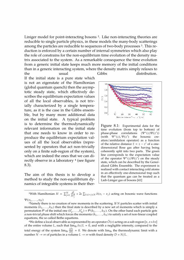
Liniger model for point-interacting bosons 2. Like non-interacting theories arereducible to single particle physics, in these models the many-body scatteringsamong the particles are reducible to sequences of two-body processes 3. This re-duction is enforced by a certain number of internal symmetries which also playthe role of constrains for the non-equilibrium time evolution of the density ma-trix associated to the system. As a remarkable consequence the time evolutionfrom a generic initial state keeps much more memory of the initial conditionsthan in a generic interacting system, where the density matrix simply relaxes tothe usual Gibbs distribution.
Figure 8.1: Experimental data for thetime evolution (from top to bottom) ofphase-phase correlations 〈Ψ+(z)Ψ(z′)〉(with Ψ+(z),Ψ(z′) the bosonic cre-ation/annhilation operator) as a functionof the relative distance z z − z′ of a one-dimensional Bose gas after having beingcoherently split into two parts. The greenline corresponds to the expectation valueof the operator Ψ+(z)Ψ(z′) on the steadystate, which can be described by the Gener-alized Gibbs Ensemble. The experiment isrealized with contact interacting cold atomsin an eectively one-dimensional trap suchthat the quantum gas can be treated as aLieb-Liniger gas of bosons [41]
If the initial state is a pure state whichis not an eigenstate of the Hamiltonian(global quantum quench) then the asymp-totic steady state, which eectively de-scribes the equilibrium expectation valuesof all the local observables, is not triv-ially characterized by a single tempera-ture, as it is the case in the Gibbs ensem-ble, but by many more additional dataon the initial state. A typical problemis to determine the thermodynamicallyrelevant information on the initial statethat one needs to know in order to re-produce the equilibrium expectation val-ues of all the local observables (repre-sented by operators that act non-triviallyonly on a nite sub-region of the system),which are indeed the ones that we can di-rectly observe in a laboratory 4 (see gure8.3).
The aim of this thesis is to develop amethod to study the non-equilibrium dy-namics of integrable systems in their ther-
2With Hamiltonian H ∑N
j1∂2
∂x2j+ 2c
∑1≤i< j≤N δ(xi − x j ) acting on bosonic wave functions
Ψ(x1 , . . . , xN )3Namely there is no creation of new momenta in the scattering. If N particles scatter with initial
momenta (k1 , . . . , kN ) then the nal state is described by a new set of momenta which is simply apermutation P of the initial one (k′1 , . . . , k
′
N ) P(k1 , . . . , kN ). On the other hand each particle getsa non-trivial phase shift which forces the momenta (k1 , . . . , kN ) to satisfy a set of non-linear coupledequations, the so called Bethe equations.
4Wedene a local observable as represented by an operator O(x) acting on a sub-region [x , x+δx]of the entire volume L, such that limth δx/L 0, and with a negligible intensity, compared to thetotal energy of the system limth
〈O〉〈H〉 0. We denote with limth the thermodynamic limit with a
number N →∞ of particles in a volume L →∞with xed density D N/L.
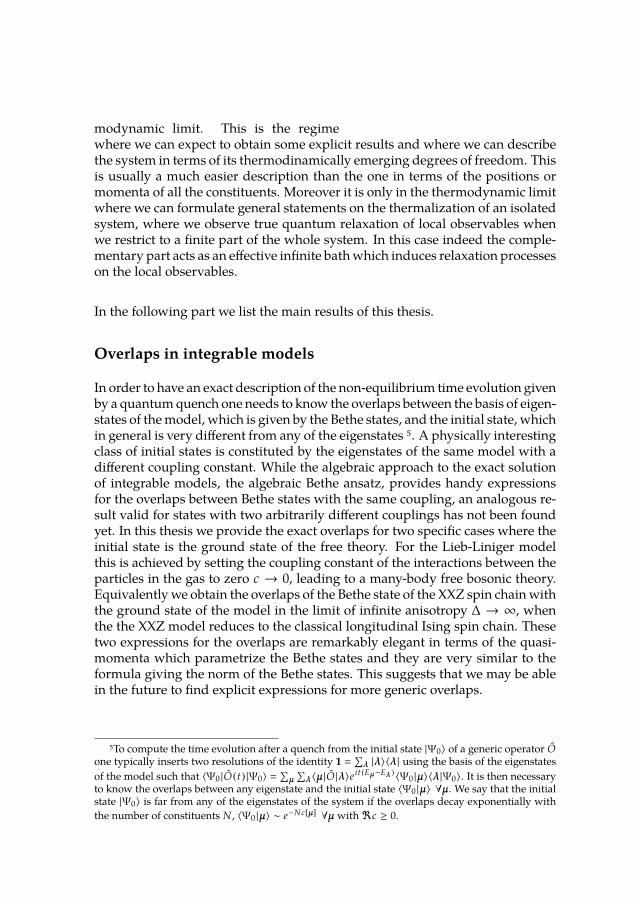
modynamic limit. This is the regimewhere we can expect to obtain some explicit results and where we can describethe system in terms of its thermodinamically emerging degrees of freedom. Thisis usually a much easier description than the one in terms of the positions ormomenta of all the constituents. Moreover it is only in the thermodynamic limitwhere we can formulate general statements on the thermalization of an isolatedsystem, where we observe true quantum relaxation of local observables whenwe restrict to a nite part of the whole system. In this case indeed the comple-mentary part acts as an eective innite bathwhich induces relaxation processeson the local observables.
In the following part we list the main results of this thesis.
Overlaps in integrable models
In order to have an exact description of the non-equilibrium time evolution givenby a quantumquench one needs to know the overlaps between the basis of eigen-states of themodel, which is given by the Bethe states, and the initial state, whichin general is very dierent from any of the eigenstates 5. A physically interestingclass of initial states is constituted by the eigenstates of the same model with adierent coupling constant. While the algebraic approach to the exact solutionof integrable models, the algebraic Bethe ansatz, provides handy expressionsfor the overlaps between Bethe states with the same coupling, an analogous re-sult valid for states with two arbitrarily dierent couplings has not been foundyet. In this thesis we provide the exact overlaps for two specic cases where theinitial state is the ground state of the free theory. For the Lieb-Liniger modelthis is achieved by setting the coupling constant of the interactions between theparticles in the gas to zero c → 0, leading to a many-body free bosonic theory.Equivalentlywe obtain the overlaps of the Bethe state of the XXZ spin chainwiththe ground state of the model in the limit of innite anisotropy ∆ → ∞, whenthe the XXZ model reduces to the classical longitudinal Ising spin chain. Thesetwo expressions for the overlaps are remarkably elegant in terms of the quasi-momenta which parametrize the Bethe states and they are very similar to theformula giving the norm of the Bethe states. This suggests that we may be ablein the future to nd explicit expressions for more generic overlaps.
5To compute the time evolution after a quench from the initial state |Ψ0〉 of a generic operator Oone typically inserts two resolutions of the identity 1
∑λ |λ〉〈λ | using the basis of the eigenstates
of the model such that 〈Ψ0 |O(t) |Ψ0〉 ∑µ∑λ 〈µ|O |λ〉e
it(Eµ−Eλ )〈Ψ0 |µ〉〈λ |Ψ0〉. It is then necessary
to know the overlaps between any eigenstate and the initial state 〈Ψ0 |µ〉 ∀µ. We say that the initialstate |Ψ0〉 is far from any of the eigenstates of the system if the overlaps decay exponentially withthe number of constituents N , 〈Ψ0 |µ〉 ∼ e−Nc[µ]
∀µ with<c ≥ 0.
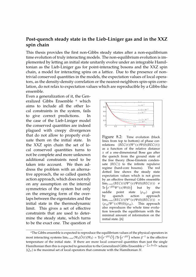
Post-quench steady state in the Lieb-Liniger gas and in the XXZspin chainThis thesis provides the rst non-Gibbs steady states after a non-equilibriumtime evolution of truly interactingmodels. The non-equilibrium evolution is im-plemented by letting an initial state unitarily evolve under an integrable Hamil-tonian as the Lieb-Liniger gas for point-interacting bosons and the XXZ spinchain, a model for interacting spins on a lattice. Due to the presence of non-trivial conserved quantities in the models, the expectation values of local opera-tors, as the density-density correlation or the nearest-neighbors spin-spin corre-lation, do not relax to expectation values which are reproducible by a Gibbs-likeensemble.
0
0.2
0.4
0.6
0.8
1
0 0.5 1 1.5 2 2.5
x
t = 10−1
t = 10−2
t = 10−3
t = 5× 10⁻²
t = 5× 10⁻³
t = 0
Figure 8.2: Time evolution (blacklines from top to bottom) of phase cor-relations 〈BEC(t) |Ψ+(x)Ψ(0) |BEC(t)〉as a function of the relative distancex of a one-dimensional Bose gas afterthe quench from the ground state ofthe free theory (Bose-Einstein conden-sate |BEC〉) to the innite repulsiveregime (hard-core bosons). The reddotted line shows the steady stateexpectation values which is not givenby an eective thermal Gibbs ensemblelimt→∞〈BEC(t) |Ψ+(x)Ψ(0) |BEC(t)〉 ,Tr
(e−βHΨ+(x)Ψ(0)
)but by the
saddle point state |ρsp〉 givenby quench action approachlimt→∞〈BEC(t) |Ψ+(x)Ψ(0) |BEC(t)〉
〈ρsp |Ψ+(x)Ψ(0) |ρsp〉. This approach
also reproduces the whole time evolu-tion towards the equilibrium with theminimal amount of information on theinitial state. [6]
Even a generalization of it, the Gen-eralized Gibbs Ensemble 6 whichaims to include all the other lo-cal constraints in the system, failsto give correct predictions. Inthe case of the Lieb-Liniger modelthe conserved quantities are indeedplagued with creepy divergencesthat do not allow to properly eval-uate them on the initial state. Inthe XXZ spin chain the set of lo-cal conserved quantities turns tonot be complete and more unknownadditional constraints need to betaken into account. We then ad-dress the problem with an alterna-tive approach, the so called quenchaction approach, which does not relyon any assumption on the internalsymmetries of the system but onlyon the emerging form of the over-laps between the eigenstates and theinitial state in the thermodynamiclimit. This gives a set of eectiveconstraints that are used to deter-mine the steady state, which turnsto be the exact one. The question of
6The Gibbs ensemble is expected to reproduce the equilibrium values of the physical operators inmost interacting systems limt→∞〈Ψ0 |O(t) |Ψ0〉 Tr
(e−βH O
)/Tr
(e−βH
)where β−1 is the eective
temperature of the initial state. If there are more local conserved quantities than just the singleHamiltonian then this is expected to generalize to the GeneralizedGibbs Ensemble e−
∑n βn Qn where
Qn is the maximal set of local operators that commute with the Hamiltonian H.

how to reproduce such exact steadystates with the alternative approach of the Generalized Gibbs Ensemble is notanswered yet.
Time evolutionWhile some facts on the steady state after a non-equilibrium time evolution arein general established, on the contrarymuch less is known on the time evolutiontowards equilibrium. This is in general a much more complicated problem. Aquite common statement for example is that in order to reproduce its whole timeevolution a larger amount of information on the initial state is needed, comparedto the one necessary to reconstruct the steady state at innite times. However weshow in this thesis that this is not the case in a quenched integrable model (seegure 8.4). The thermodynamic limit indeed selects only a restricted amount ofdata on the initial state, which are responsible for the whole time evolution upto innite times, when the system has relaxed to its steady state. This is a directconsequence of the quench action approach, which also provides a general toolto access the eective time scales of the non-equilibrium dynamics which areencoded in the post-quench eective velocity of propagation of the excitations.This is also a functional of the initial state and does not depend on all its detailsbut only on its macroscopic parameters (like its energy density for example).Dierent initial states therefore will lead to eective eld theories with dierentlight velocities.Besides its theoretical relevance the whole time evolution is also much morerelated to experimental realizations. Cold atoms experiments are indeed usuallylimited in the range of time, making usually impossible to observe the true post-quench steady state in a real setting (See gure 8.3).

Samenvatting
Sinds het ontstaan van de wetenschappelijke methode is over de gehele linievan de exacte wetenschappen het idee geaccepteerd dat om de natuur te kun-nen begrijpen zij ontleed moet worden tot haar elementaire bestanddelen. Ookal leidde deze overtuiging tot immense ontdekkingen op het gebied van de sub-atomische deeltjes, waaruit een geüniceerde theorie van elektromagnetisme,de zwakke en sterke krachten binnen een atoomkern (het zogeheten standaardmodel) ontstond, toch kon het andere grote vraagstukken niet beantwoorden.Neem bijvoorbeeld emergentie wat één van de meest fascinerende conceptenbinnen de moderne fysica is. Emergentie is het proces waarbij ingewikkeldemacroscopische eigenschappen voortkomen uit de interacties tussen vele, zichsimpel gedragende, bestanddelen. Beschouw bijvoorbeeld een systeem waarbijde interacties tussen de afzonderlijke bestanddelen erg grootworden, dan zullende eigenschappen van het gehele systeem totaal verschillen van de eigenschap-pen van één op zichzelf staand bestanddeel. Nieuwe nog niet eerder ontdektenatuurkunde verrijst uit de aanwezigheid van deze niet-triviale interacties dieover het algemeen niet perturbatief kunnen worden behandeld. Daarmee wordtbedoeld dat er in de analyse niet mag worden aangenomen dat de interactiesheel klein zijn. Wanneer de bestanddelen zich bijvoorbeeld alleen maar binneneen één-dimensionale geometrie mogen bewegen, worden de interacties meereectief, oftewel belangrijker. Het verkeer op een weg met maar één rijbaan,kan overgaan van vloeibaar naar verstopt, door de dichtheid van auto’s net ietsgroter te maken dan een bepaalde kritische waarde. Op dezelfde manier zijnde bewegingen in één dimensie van veel quantum deeltjes bij elkaar die een on-derlinge interactie hebben collectief en gedragen zij zich dus als een vloeistof.Wanneer zij in een situatie buiten equilibrium worden geprepareerd, zullen zijzich reorganiseren op een ongebruikelijke en moeilijk te voorspellen manier diemogelijk kan leiden tot nieuwe exotische toestanden der materie.
Quantum systemen bestaande uit een groot aantal bestanddelen met sterke on-derlinge interacties zijn over het algemeen erg moeilijk om te behandelen. Omeen quantummechanisch probleem op te lossenmoetmen theHamiltoniaan diehet systeem omschrijft diagonaliseren. DezeHamiltoniaan is eenmatrixmet de-zelfde dimensie als de Hilbert ruimte en groeit exponentieel met het aantal ele-mentaire deeltjes N waaruit het systeem bestaat. Het onderzoek naar quantumsystemen in equilibrium maakt gebruik van een aantal instrumenten die ofwelgebruik maken van de zwakte van de interactie zoals bij perturbatie theorie, of-wel van een beschrijving waarbij er wordt uitgegaan dat de uctuaties van defysische observabelen rond hunwaarde in equilibrium klein zijn zoals bij mean-eld benaderingen.
173

Deze manieren van aanpak zijn afhankelijk van zekere aannames die zelden ge-controleerd kunnenwordenmet een exacte oplossing voor ieder mogelijk aantaldeeltjes N . Maar wanneer we slechts één-dimensionale systemen beschouwenblijkt hetwélmogelijk te zijn omexacte oplossingen te vinden voormodellenmetinteracties en die ook nog eens fysiek relevant zijn.
Figuur 8.3: Experimentele data voorde tijdsevolutie (van boven naar bene-den gezien) van de fase-fasecorrelaties〈Ψ†(z)Ψ(z′)〉 (waarbijΨ†,Ψ de bosonischecreatie/annihilatie operatoren zijn) als eenfunctie van de relatieve afstand z z − z′van een één-dimensionaal Bose gas nadathet op coherente wijze in twee delen isopgesplitst. Het experiment wordt gere-aliseerd met koude atomen die interactiehebben via contact en zich bevinden in eeneectief één-dimensionale val zodanig dathet quantum gas beschouwd kan wordenals een Lieb-Liniger gas van bosonen [41].
Deze modellen worden integreerbaar ge-noemd en twee voorbeelden, die behan-deld worden in dit proefschrift, zijn deXXZ Heisenberg spin keten 7 en het Lieb-Liniger model voor bosonen met punt-interacties 8. Net zoals theorieën zon-der interactie teruggebracht kunnen wor-den tot één-deeltjes fysica, zo kunnen bijdeze modellen de veel-deeltjes verstrooi-ing teruggebracht worden tot series vantwee-deeltjes interacties 9. Deze reduc-tie wordt opgelegd door een aantal in-terne symmetrieën. Deze spelen boven-dien de rol van randvoorwaarden op deniet-equilibrium tijdsevolutie van de dicht-heidsmatrix die bij het systeem hoort. Eenopvallende consequentie hiervan is dat detijdsevolutie van een generieke begintoe-stand veel meer geheugen bezit van debegincondities dan het geval is bij eengeneriek systeem met interacties, waarbijde dichtheidsmatrix simpelweg relaxeertnaar het gebruikelijke Gibbs ensemble. Als de begintoestand een pure toestandis en geen eigentoestand van de Hamiltoniaan (globale quantum quench) danwordt de asymptotische evenwichtstoestand, welke de verwachtingswaardenvan de alle lokale observabelen in equilibrium beschrijft, niet triviaal gekarak-teriseerd door één enkele temperatuur zoals het geval is voor het Gibbs ensem-ble, maar door veel meer extra informatie over de begintoestand. Een standaard
7Met Hamiltoniaan H J∑L
j1
(σx
j σxj+1 + σ
yj σ
yj+1 + ∆σ
zj σ
zj+1
), waarbij σαj de Pauli matrices zijn
die geassocieerd worden met iedere spin op het rooster.8Met Hamiltoniaan H
∑Nj1
∂2
∂x2j+ 2c
∑1≤i< j≤N δ(xi − x j ) die werkt op bosonische goluncties
Ψ(x1 , . . . , xN ).9Er is namelijk geen creatie van nieuwe momenta bij deze verstrooiingen. Als N deeltjes
verstrooien met beginmomenta (k1 , . . . , kN ) dan kan de eindtoestand beschreven worden dooreen nieuwe verzameling van momenta die simpelweg een permutatie P is van de begintoestand(k′1 , . . . , k
′
N ) P(k1 , . . . , kN ). Aan de andere kant krijgt ieder deeltje een niet-triviale faseverschui-ving tijdens het verstrooiingsproces wat er voor zorgt dat de momenta (k1 , . . . , kN ) aan een verza-meling niet-lineaire gekoppelde vergelijkingen moeten voldoen, de zogeheten Bethe vergelijkingen.
vraagstuk in deze context is het vaststellen van de thermodynamische relevanteinformatie over de begintoestand die men zal moeten achterhalen om de equili-brium verwachtingswaarden van alle lokale observabelen vast te kunnen stellen(gerepresenteerd door operatoren die niet-triviaal op slechts een eindige subre-gion van het systeem werken). Dit zijn degene die we direct in het laboratoriumkunnen observeren 10 (zie guur 8.3).
Het doel van dit proefschrift is om een methode te ontwikkelen om de niet-equilibrium dynamica van integreerbare systemen te bestuderen in hun ther-modynamische limiet. In dit regime kunnen we enkele expliciete resultatenverwachten, aangezien we het systeem kunnen beschrijven in termen van dethermodynamisch emergerende vrijheidsgraden. Over het algemeen is dit eenmakkelijkere beschrijving dan die in termen van posities en momenta van alledeeltjes. Bovendien kunnenwe slechts in de thermodynamische limiet algemeneopmerkingen maken over de thermalisatie van een geïsoleerd systeem. We ob-serveren inderdaad alleen een perfecte relaxatie van de lokale observabelen alshet aantal deeltjes in het systeem naar oneindig gaat. Wanneer we in deze limietslechts een eindig deel van het gehele systeem bekijken, dan zal het complemen-taire deel zich gedragen als een eectief oneindig bad wat relaxatie processenvan de lokalen observabelen induceert.
In het volgende deel zullen we de belangrijkste resultaten uit dit proefschriftnoemen.
Overlappen in integreerbare modellenOm een exacte beschrijving te krijgen van de niet-equilibrium tijdsevolutie ge-geven door een quantum quench, zal men de overlap moeten vinden tussen debasis van eigentoestanden van het model, gegeven door de Bethe toestanden, ende begintoestand, welke in het algemeen erg verschilt van alle eigentoestanden11. Een fysisch interessante groep van begintoestanden zijn de eigentoestandenvan het model met verschillende koppelingsconstanten. Zoals de algebraïschemethode om de exacte oplossing van integreerbare modellen te vinden, de alge-braïsche Bethe ansatz, handige uitdrukkingen geeft voor de overlappen tussen
10We deniëren een lokale observabele als de actie van een operator O(x) die werkt op een ge-deelte [x , x + δx] van het gehele volume L, zodanig dat limth δx/L 0, en met een verwaarloosbareintensiteit in vergelijking met de totale energie van het systeem limth
〈O〉〈H〉 0. Met limth bedoelen
we de thermodynamische limiet waarbij het aantal deeltjes N →∞ in een volume L →∞ terwijl dedichtheid constant is D N/L.
11Om de tijdsevolutie na een quench te berekenen van de begintoestand |Ψ0〉 van een generiekeoperator O, zal men over het algemeen tweemaal de identiteitsoperator 1
∑λ |λ〉〈λ | invullen door
gebruik te maken van de basis van eigentoestanden van het model zodanig dat 〈Ψ0 |O(t) |Ψ0〉 ∑µ∑λ 〈µ|O |λ〉e
it(Eµ−Eλ )〈Ψ0 |µ〉〈λ |Ψ0〉. Vervolgens moet men alle overlappen kennen voor iedere
eigentoestand 〈Ψ0 |µ〉∀µ. We karakteriseren de begintoestand |Ψ0〉 als ver verwijderd van alle eigen-toestanden van het systeem als de overlappen exponentieel afnemenmet het aantal bestanddelen N ,〈Ψ0 |µ〉 ∼ e−Nc[µ]
∀µ met<c ≥ 0.
twee arbitraire Bethe toestanden met dezelfde koppelingsconstante, zo is eenanaloog resultaat voor toestanden met twee verschillende koppelingsconstan-ten nog niet bekend. In dit proefschrift gevenwe de exacte overlappen voor tweespecieke gevallenwaarbij de begintoestand de grondtoestand van een vrije the-orie is. Voor het Lieb-Liniger model wordt dit bereikt door de koppelingscon-stante van de interacties tussen de deeltjes in het gas op nul te zetten c → 0,wat resulteert in een veel-deeltjes vrije bosonische theorie. Op dezelfde wijzevinden we de overlappen van de Bethe toestanden voor de XXZ spin keten metde grondtoestand van het model in de limiet van oneindige anisotropie ∆→∞,waarin het XXZmodel reduceert tot de klassieke longitudinale Ising spin keten.Deze twee uitdrukkingen voor de overlappen zijn opvallend elegant in termenvan de quasimomenta die de Bethe toestanden parametriseren en ze lijken ergop de formule die de norm van iedere Bethe toestand geeft. Dit suggereert datwe in de toekomst wellicht expliciete formules voor meer generieke overlappenkunnen vinden.
Post-quench evenwichtstoestand in het Lieb-Liniger gas en in deXXZ spin ketenDit proefschrift geeft de eerste niet-Gibbs evenwichtstoestand na een niet-equilibrium tijdsevolutie vanmodellenmet interactie. De niet-equilibrium evo-lutie wordt geïmplementeerd door een begintoestand op unitaire wijze te la-ten evolueren onder een integreerbare Hamiltoniaan, zoals het Lieb-Liniger gasvoor bosonen met punt-interactie en de XXZ spin keten, een model voor spinsmet interacties op een rooster. Door de aanwezigheid van niet-triviale behoudengrootheden in de modellen, relaxeren de verwachtingswaarden van lokale ope-ratoren, zoals de dichtheids-dichtheidscorrelatie of de nearest-neighbors spin-spincorrelatie, niet naar de verwachtingswaarden die reproduceerbaar zijn dooreenGibbs-achtig ensemble. Zelfs een generalisatie hiervan, hetGegeneraliseerdeGibbs Ensemble 12 die probeert om al de andere lokale randvoorwaarden in hetsysteem op te nemen, faalt in het geven van correcte voorspellingen. In het ge-val van het Lieb-Liniger model zien we inderdaad dat de behouden groothedengeplaagd worden door vervelende divergenties waardoor ze niet geëvalueerdkunnen worden op de begintoestand. Binnen de XXZ spin keten blijkt de ver-zameling lokale grootheden niet volledig te zijn, waardoor er meer onbekendeextra randvoorwaarden meegenomen moeten worden. We adresseren het pro-bleem met een alternatieve aanpak, de zogeheten quench actie aanpak, die nietafhankelijk is van enige aanname omtrent de interne symmetrieën van het sys-teem, maar slechts van de verrijsende vorm van de overlappen tussen de eigen-
12Het Gibbs ensemble zou de equilibrium waarden van de fysische operatoren in de meeste sys-temen met interacties moeten reproduceren limt→∞〈Ψ0 |O(t) |Ψ0〉 Tr
(e−βH O
)/Tr
(e−βH
)waarbij
β−1 de eectieve temperatuur van de begintoestand is. Zodra er meer lokale behouden groothedenzijn dan slechts de Hamiltoniaan, zal het gegeneraliseerdmoeten worden naar het GengeneraliseerdGibbs Ensemble e−
∑n βn Qn waarbij Qn demaximale verzameling van lokale operatoren is die com-
muteren met de Hamiltoniaan H.
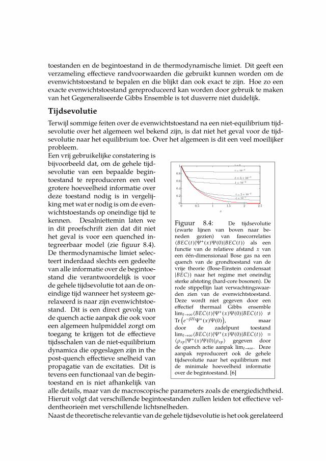
toestanden en de begintoestand in de thermodynamische limiet. Dit geeft eenverzameling eectieve randvoorwaarden die gebruikt kunnen worden om deevenwichtstoestand te bepalen en die blijkt dan ook exact te zijn. Hoe zo eenexacte evenwichtstoestand gereproduceerd kan worden door gebruik te makenvan het Gegeneraliseerde Gibbs Ensemble is tot dusverre niet duidelijk.
TijdsevolutieTerwijl sommige feiten over de evenwichtstoestand na een niet-equilibrium tijd-sevolutie over het algemeen wel bekend zijn, is dat niet het geval voor de tijd-sevolutie naar het equilibrium toe. Over het algemeen is dit een veel moeilijkerprobleem.
0
0.2
0.4
0.6
0.8
1
0 0.5 1 1.5 2 2.5
x
t = 10−1
t = 10−2
t = 10−3
t = 5× 10⁻²
t = 5× 10⁻³
t = 0
Figuur 8.4: De tijdsevolutie(zwarte lijnen van boven naar be-neden gezien) van fasecorrelaties〈BEC(t) |Ψ+(x)Ψ(0) |BEC(t)〉 als eenfunctie van de relatieve afstand x vaneen één-dimensionaal Bose gas na eenquench van de grondtoestand van devrije theorie (Bose-Einstein condensaat|BEC〉) naar het regime met oneindigsterke afstoting (hard-core bosonen). Derode stippellijn laat verwachtingswaar-den zien van de evenwichtstoestand.Deze wordt niet gegeven door eeneectief thermaal Gibbs ensemblelimt→∞〈BEC(t) |Ψ+(x)Ψ(0) |BEC(t)〉 ,Tr
(e−βHΨ+(x)Ψ(0)
), maar
door de zadelpunt toestandlimt→∞〈BEC(t) |Ψ+(x)Ψ(0) |BEC(t)〉
〈ρsp |Ψ+(x)Ψ(0) |ρsp〉 gegeven door
de quench actie aanpak limt→∞. Dezeaanpak reproduceert ook de geheletijdsevolutie naar het equilibrium metde minimale hoeveelheid informatieover de begintoestand. [6]
Een vrij gebruikelijke constatering isbijvoorbeeld dat, om de gehele tijd-sevolutie van een bepaalde begin-toestand te reproduceren een veelgrotere hoeveelheid informatie overdeze toestand nodig is in vergelij-kingmetwat er nodig is omde even-wichtstoestands op oneindige tijd tekennen. Desalniettemin laten wein dit proefschrift zien dat dit niethet geval is voor een quenched in-tegreerbaar model (zie guur 8.4).De thermodynamische limiet selec-teert inderdaad slechts een gedeeltevan alle informatie over de begintoe-stand die verantwoordelijk is voorde gehele tijdsevolutie tot aan de on-eindige tijd wanneer het systeem ge-relaxeerd is naar zijn evenwichtstoe-stand. Dit is een direct gevolg vande quench actie aanpak die ook vooreen algemeen hulpmiddel zorgt omtoegang te krijgen tot de eectievetijdsschalen van de niet-equilibriumdynamica die opgeslagen zijn in thepost-quench eectieve snelheid vanpropagatie van de excitaties. Dit istevens een functionaal van de begin-toestand en is niet afhankelijk vanalle details, maar van de macroscopische parameters zoals de energiedichtheid.Hieruit volgt dat verschillende begintoestanden zullen leiden tot eectieve vel-dentheorieën met verschillende lichtsnelheden.Naast de theoretische relevantie vande gehele tijdsevolutie is het ook gerelateerd
aan experimentele realisaties. Experimentenmet koude atomen zijn namelijk ge-limiteerd in tijdsspanne, daaruit volgt dat het observeren van een evenwichtstoe-stand die ontstaat na een oneindige tijd nadat de quench heeft plaatsgevonden,hopeloos is in een echte context (zie guur 8.3).
179

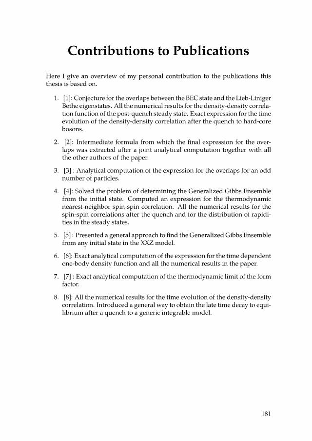
Contributions to Publications
Here I give an overview of my personal contribution to the publications thisthesis is based on.
1. [1]: Conjecture for the overlaps between the BEC state and the Lieb-LinigerBethe eigenstates. All the numerical results for the density-density correla-tion function of the post-quench steady state. Exact expression for the timeevolution of the density-density correlation after the quench to hard-corebosons.
2. [2]: Intermediate formula from which the nal expression for the over-laps was extracted after a joint analytical computation together with allthe other authors of the paper.
3. [3] : Analytical computation of the expression for the overlaps for an oddnumber of particles.
4. [4]: Solved the problem of determining the Generalized Gibbs Ensemblefrom the initial state. Computed an expression for the thermodynamicnearest-neighbor spin-spin correlation. All the numerical results for thespin-spin correlations after the quench and for the distribution of rapidi-ties in the steady states.
5. [5] : Presented a general approach to nd theGeneralizedGibbs Ensemblefrom any initial state in the XXZ model.
6. [6]: Exact analytical computation of the expression for the time dependentone-body density function and all the numerical results in the paper.
7. [7] : Exact analytical computation of the thermodynamic limit of the formfactor.
8. [8]: All the numerical results for the time evolution of the density-densitycorrelation. Introduced a general way to obtain the late time decay to equi-librium after a quench to a generic integrable model.
181


Acknowledgments
The idea of writing a PhD thesis is usually overwhelming as it requires to lookback at the last four years and to summarize everything it has been done. In mycase this job has not been particularly easy since I am an awful book-keeper, mynotes are always pretty bad and I rarely write things down, with the excuse thateverything will stay forever in my mind. Well, partially it is true. For example Iremember quite vividly the rst day I walked in Science Park, and how warmlyI was welcomed. My supervisor Jean-Sébastien accepted me from the very rstday as one of his students and friends, as we knew each other since long time.Eventually I found in him an excellent teacher, a true friend, a fair colleague andnally a trustworthy mentor. The numerous enlightening conversations we hadin these past years showed me his admirable attitude towards physics and anyaspects of life, inuencing me deeply. I consider having been one of his studentsa big fortune. Thank you J-S.
On the other hand, the high quality of life at the Institute of Physics was also dueto the beautiful people there. Kareljan, Vladimir and Jan have always been readyto help and give precious suggestions. It was a pleasure to be Bernard’s teachingassistant and nally it has been quite inspiring to meet the new young people,Katerina, Florian, Philippe and Jasper. Anne-Marieke, Fatima, Natalie, Joost andYocklang made my arrival and my permanence easy and pleasant. Thank youfor having replied to all my annoying emails and always having found the timeto take care of all my issues.
I had been lucky enough to live the golden time of the one-dimensional gang. Ihad such a great time together with Sebas, Thessa, Miłosz, Jorn, Bram, Rogier,Rianne, Giuseppe, Davide, Omar, Michael and nally Enej. I like to think ofourselves as the "Via Panisperna Boys", eager to think always about new stuand creating great things together (but with dierent consequences hopefully).Sebas and Thessa have been great oce mates with whom to share frustrationsand cold summer days in the oce. Thank you Sebas for having told me all Iknow about eld theory and cool places in the city. Thank you Rianne for ourheroic escalades done while talking about future projects. It has been a greatpleasure to work with Bram, Enej and Michael, whose patience and order wellcounterbalanced my impulsiveness and messiness. Thank you guys for havingtaught me so much. Thank you Miłosz, with you I shared beautiful road trips,loads of laughs and love for Bethe Ansatz.
Four years in Amsterdam have gone too quickly. They say that time ies whenyou are having fun. If this had been the case it is mostly due to the amazingpeople I have met there: Sabrina, Shanna, Lau, Annelise, György, Milena, Nico-las, Benedetta, Goredo, Michael (the danish), Mathilde, Ali, Abdo, Holiday,
183

Philip, Antoine, Inge, Balazs, Daniel, Natasha, Johannes, Luciano, Marco, Ana,Moos, Benjamin, Giulia, Peo. Arnica, youmademe live the magic of theater andof wine-based therapy evenings, you contributed a lot to this work. Nachiket, Ithink this is the beginning of a beautiful friendship (andwe’ll always have Paris).Finally in order to properly thank Hélène I may quote Brassens: "a la compagnede voyage, dont les yeux, charmant paysage, font paraître court le chemin".
This thesis is supposed to contain four years of life. But life is a continuous pro-cess and it can not be easily divided into boxes. Therefore the people who havealways been inmyow, largely inuencing and guiding it, must be remembered.Claudia e Mirko, my second family, hard to say in words I much I owe you. Mayyou stay forever young, my beloved friends.
I own a large part of this work and of myself to my dear parents, Carla e Paolo,to my big-big brother, Andrea with his new beautiful family and nally to mygrandparents, the ones are gone already and the one is still here.Questo libro è dedicato a voi, spero vi sia piaciuto.