UvA-DARE (Digital Academic Repository) Sparse-Grid … · Sparse-Grid Finite-Volume Multigrid for 3D-Problems ... Sparse-grid finite-volume multigrid for 3D ... algorithm for the

UvA-DARE is a service provided by the library of the University of Amsterdam (http://dare.uva.nl)

UvA-DARE (Digital Academic Repository)

Sparse-Grid Finite-Volume Multigrid for 3D-Problems

Hemker, P.W.

Published in:Advances in Computational Mathematics

Link to publication

Citation for published version (APA):Hemker, P. W. (1995). Sparse-Grid Finite-Volume Multigrid for 3D-Problems. Advances in ComputationalMathematics, 4, 83-110.

General rightsIt is not permitted to download or to forward/distribute the text or part of it without the consent of the author(s) and/or copyright holder(s),other than for strictly personal, individual use, unless the work is under an open content license (like Creative Commons).

Disclaimer/Complaints regulationsIf you believe that digital publication of certain material infringes any of your rights or (privacy) interests, please let the Library know, statingyour reasons. In case of a legitimate complaint, the Library will make the material inaccessible and/or remove it from the website. Please Askthe Library: http://uba.uva.nl/en/contact, or a letter to: Library of the University of Amsterdam, Secretariat, Singel 425, 1012 WP Amsterdam,The Netherlands. You will be contacted as soon as possible.

Download date: 17 Oct 2017

http://dare.uva.nl/personal/pure/en/publications/sparsegrid-finitevolume-multigrid-for-3dproblems(320fd13d-adb6-42d6-81ed-072d38854a86).html

Advances in Computational Mathematics 4(1995)83-110 83

Sparse-grid finite-volume multigrid for 3D-problems

P.W. H e m k e r

Centrum voor Wiskunde en Informatica, P.O. Box 94079, 1090 GB Amsterdam, The Netherlands

We introduce a multigrid algorithm for the solution of a second order elliptic equation in three dimensions. For the approximation of the solution we use a partially ordered hierarchy of finite-volume discretisations. We show that there is a relation with semicoarsening and approximation by more-dimensional Haar wavelets. By taking a proper subset of all possible meshes in the hierarchy, a sparse grid finite-volume discretisation can be constructed.

The multigrid algorithm consists of a simple damped point-Jacobi relaxation as the smoothing procedure, while the coarse grid correction is made by interpolation from several coarser grid levels.

The combination of sparse grids and multigrid with semi-coarsening leads to a relatively small number of degrees of freedom, N, to obtain an accurate approximation, together with an O(N) method for the solution. The algorithm is symmetric with respect to the three coordinate directions and it is fit for combination with adaptive techniques.

To analyse the convergence of the multigrid algorithm we develop the necessary Fourier analysis tools. All techniques, designed for 3D-problems, can also be applied for the 2D case, and - for simplicity - we apply the tools to study the convergence behaviour for the anisotropic Poisson equation for this 2D case.

Keywords: Sparse grids, multigrid, finite volume, discrete Fourier transform, wavelets.

AMS subject classification: 65N55, 65N22, 65T20.

1. I n t r o d u c t i o n

In this pape r we describe the a p p r o x i m a t i o n o f a func t ion on a f ini te-volume sparse grid, and a mul t igr id a lgor i thm for the solut ion o f par t ia l differential equa t ions in three dimensions . The a lgor i thm is in tended for the solut ion o f flow prob lems descr ibed by conse rva t ion laws, and the re fore finite volumes are a na tura l choice for the discret isat ion. But to in t roduce the ma in principles, we will restr ict the t r ea tmen t here to second o rde r elliptic equat ions , and in par t icu la r to the an iso t rop ic Po isson equat ion .

In con t ras t to the usual mul t igr id approach , we do no t use a sequential ly o rde red set o f discret isat ions on different meshes, bu t we use a par t ia l ly o rde red h ie ra rchy o f " s emi -coa r sened" grids as p r o p o s e d e.g. by M u l d e r [6,7] and N a i k - V a n R o s e n d a l e [8] or Zenger et al. [3,9]. As indicated in [9], adap t ive " spa r se -g r id" discret isat ions

© J.C. Baltzer AG, Science Publishers

84 P. IV. Hemker / Sparse-grid finite-volume multigrid

can be constructed by taking a suitable subset of all possible discretisations in such a hierarchy. However, in contrast to the sparse grid approximat ion proposed in [3,9], we base our approximat ion on finite volumes rather than on finite elements.

The multigrid algori thm consists of damped Jacobi relaxation as a smoothing procedure and a coarse grid correction constructed by extrapolat ion f rom simul- taneous corrections on several coarser grid levels.

The algori thm is completely symmetric with respect to the three coordinate directions and it is suitable for combinat ion with adaptive techniques. A descrip- t ion of a data structure to implement such adaptive three-dimensional algori thms is given elsewhere [5].

2. F i n i t e - v o l u m e sparse g r ids

In this section we introduce finite-volume sparse grids. We show the relation between the approximat ion by Haar wavelets (when this not ion is extended to more dimensions) and the sparse-grid approximation. For the theory of wavelets, mult iresolution analysis (MRA) etc. we refer to Daubechies [2].

2.1. The more-dimensional MRA

A multidimensional multiresolution analysis of L2(f~), ft = IR 3, is a partially ordered set of closed linear subspaces

{v. v. c with the properties:

(1) MVn= {0}; Uvn Cdense L2(a); n n

(2) f ( x ) E V, ,~=~f(2"x) E V.+m Vn E g 3, m E E; (1)

(3) f ( x ) E V, ec, f ( x - 2-"k) E V, V k E Z 3 , n E E ;

(4) 3q~ E Vo: {4~(x - k)}k~z~ is a Riesz basis for Vo.

Here n = (nl,n2,n3) E Z 3, and we denote In I = n I + n 2 -k- n3; 2 n = (2"',2"2,2"3). We also use the nota t ion o = ( 0 , 0 , 0 ) E N3; x = (xl,x2,x3)E tR3; 2"x = (2'(xl, 2~2x2,2"3x3). Further , we introduce in N 3 the unit vectors ek, k = 1, 2, 3, as follows: e l ( I ,0 ,0 ) ; e2 = (0, 1,0); e3 = (0,0, 1), and we use e = (1, 1, 1). Finally we define E = {el,ez,e3}. Al though we are particularly interested in the three- dimensional case, generalisation to a different number of space dimensions is straightforward. The function ~b(x) in (1.4) is called the sealing function of the mult iresolution analysis.

2.2. Piecewise constant function spaces

Let either [2 =]1~3 be the three-dimensional Euclidean space, or let

P.W. Hemker / Sparse-grid finite-volume multigrid 85

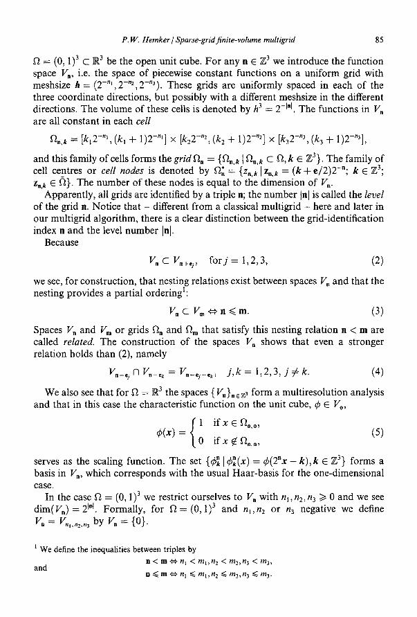
f~ = (0, 1)3 c R 3 be the open unit cube. For any n E Z 3 we introduce the function space V., i.e. the space o f piecewise constant functions on a uniform grid with meshsize h = (2-"~,2-n2,2-"3). These grids are uniformly spaced in each of the three coordinate directions, but possibly with a different meshsize in the different directions. The volume of these cells is denoted by h 3 = 2 -In[. The functions in V. are all constant in each cell

an, * = [kl2-n',(kl + 1)2-"'1 x [ke2-"2, (k2 + 1)2 -"2] x [k32-"~, (k3 + 1)2-~3],

and this family of cells forms the grid f~. = {[2~,k t fin, , C f~, k E Z3}. The family of cell centres or cell nodes is denoted by f~ = {Z~,k [Z.,t, = (k + e/2)2-"; k E Z3; Z.,k C (~}. The number of these nodes is equal to the dimension of V..

Apparently, all grids are identified by a triple n; the number Inl is called the level of the grid n, Notice that - different f rom a classical multigrid - here and later in our multigrid algorithm, there is a clear distinction between the grid-identification index n and the level number Inl.

Because

V. C Vn+ej, f o r j = 1,2,3, (2)

we see, for construction, that nesting relations exist between spaces V. and that the nesting provides a partial ordering1:

V,C V. ¢~ n ~< m. (3)

Spaces V, and Vm or grids f~. and ~"~m that satisfy this nesting relation n < m are called related. The construction of the spaces V, shows that even a stronger relation holds than (2), namely

V._ej N V._~ = V.-ej-ek, j , k = l,2,3, j C k. (4)

We also see that for f~ = IR 3 the spaces { V.}.~z3 form a mult iresolution analysis and that in this case the characteristic function on the unit cube, ~b E Vo,

1 i f x E Fro, o,

q~(x) = 0 i f x ~ f ] o , o , (5)

serves as the scaling function. The set {q~, I q~,(x) = ~b(2"x - k), k C Z 3} forms a basis in V., which corresponds with the usual Haar-basis for the one-dimensional case.

In the case f~ = (0, 1) 3 we restrict ourselves to V. with nl,n2,n3 >1 0 and we see dim(V.) = 2 tnl. Formally, for f~ = (0, 1) 3 and nl,nz or n 3 negative we define V. = V~,,.2,.3 by V. = {0}.

t W e def ine the inequa l i t i e s b e t w e e n t r iples by

n < m ¢* n I < ml~r/2 < m2~n 3 < m3~ a n d

n <~ m ¢e~ nl <<. ml,n2 <<. m2,n3 <-% rn3.

86 P.w. Hemker / Sparse-grid finite-volume multigrid

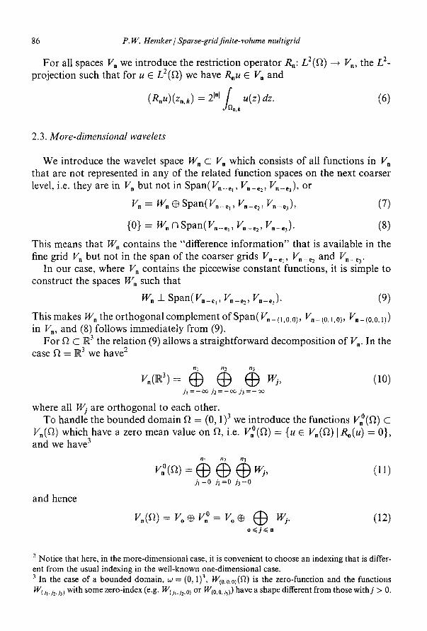
For all spaces V. we introduce the restriction operator R.: L2(f~) ---, V., the L 2- projection such that for u E L2(f~) we have R.u E V. and

(R.u)(z.,k) = 21"1~ u(z) dz. (6)

2.3. More-dimensional wavelets

We introduce the wavelet space IV. c Vn which consists of all functions in V~ that are not represented in any of the related function spaces on the next coarser level, i.e. they are in V. but not in Span(V._e, , Vn_e:, V._~), or

Vn = W. ® Span(V._~,, V._~2 , V._~), (7)

{0} = IV. n Span(V._e, , I/"._. 2, V._~3). (8)

This means that W. contains the "difference informat ion" that is available in the fine grid V. but not in the span of the coarser grids V.-e~, V.-e2 and V._e3.

In our case, where V. contains the piecewise constant functions, it is simple to construct the spaces IV. such that

IV. _1_ Span(V._, , , Vn_e2 , Vn_e3 ). (9)

This makes IV. the or thogonal complement of Span( V._ It,0,0), V._ (0, t,0/, Iv._ (0,0,1)) in V., and (8) follows immediately f rom (9).

For Sq c IR 3 the relation (9) allows a straightforward decomposi t ion of V.. In the case fl = IR 3 we have 2

t! 1 I! ~ n 3

V"(IR3)= O O ~ Wj, (10) j l = - - ~ j 2 = - - ~ j 3 = - - ~

where all IV/are or thogonal to each other. To handle the bounded domain f~ = (0, 1)3 we introduce the functions V°(f~) C

Vn(f2 ) which have a zero mean value on f~, i.e. V°(~) = {u E Vn(f~)lRo(u) = 0}, and we have 3

n I n2 n3

V ° ( ~ 2 ) = O O ~ I . V j , (11) Jl = 0 9'2=0 ,/'3=0

and hence

V n ( a ) = V o G V ° = Vo@ @ I, Vj. (12) o~<j~<n

2 Notice that here, in the more-dimensional case, it is convenient to choose an indexing that is different from the usual indexing in the well-known one-dimensional case. 3 In the case of a bounded domain, w = (0, 1) 3, W(o&o)(gt ) is the zero-function and the functions Wo.,k,J3) with some zero-index (e.g. Wij~,j,.,o) or W(o,o031) have a shape different from those withj > 0.

P.W. Hemker / Sparse-grid finite-votume multigrid 87

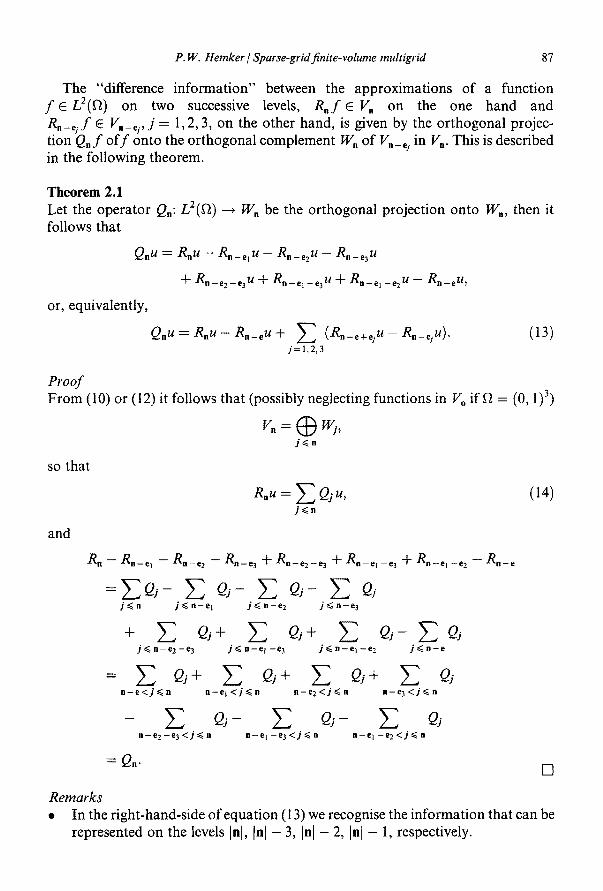
The "difference information" between the approximations of a function f EL2(~) on two successive levels, R . f E V. on the one hand and R.-e j f E V._e:,j = 1,2, 3, on the other hand, is given by the orthogonal projection Qnf o f f onto the orthogonal complement W. of V._e: in V.. This is described in the following theorem.

Theorem 2.1 Let the operator Q.: L2(f~) --, W. be the orthogonal projection onto IV., then it follows that

Q.u = Rnu - Rn_ejU - R n _ e 2 U - R n _ e 3 u

-I- Rn_e2 _e3U q- Rn_el _e3U -t- Rn_el _e2 u - - Rn_eU,

or, equivalently,

Q.u = Rnu - Rn_eU 3v Z ( R n - e + e j u - R n - e j / ' / ) " (13) j = 1,2,3

Pl'oof From (10) or (12) it follows that (possibly neglecting functions in V o if ~2 = (0, 1)3)

~.=®w.

so that

and

j<~n

RnU = E Qju, (14) j~<n

R n - Rn_e l - Rn_e2 - Rn_e3 -t- Rn_e2_e3 -~ R n - e l - e 5 + R n - e t - e z - - R n _ e

j~<n j ~ < n - e l j ~ < n - e 2 j ~ < n - e 3

+ Z Q,+ Z Q,+ Z j ~< n - e z - e 3 j ~ < n - e I - e 3 j ~< n - e | - e 2

: Z Q,+ Z; e,+ Z n - e < j ~ n n - e I < j ~ n n - e 2 < j ~ n

- E Q,- ~ Q'-- n-e2-e3 <j ~ n n-el -e3 <j<~ n

= Qn-

. Q j - Qj j ~ < n - e

n - e 3 < j ~ < n

Z Q, n--e I --e 2 < j ~< n

[]

Remarks • In the right-hand-side of equation (13) we recognise the information that can be

represented on the levels In[, In[ - 3, [n I - 2, In[ - 1, respectively.

88 P. W. H e m k e r / S p a r s e - g r i d f i n i t e - v o l u m e m u l t i g r i d

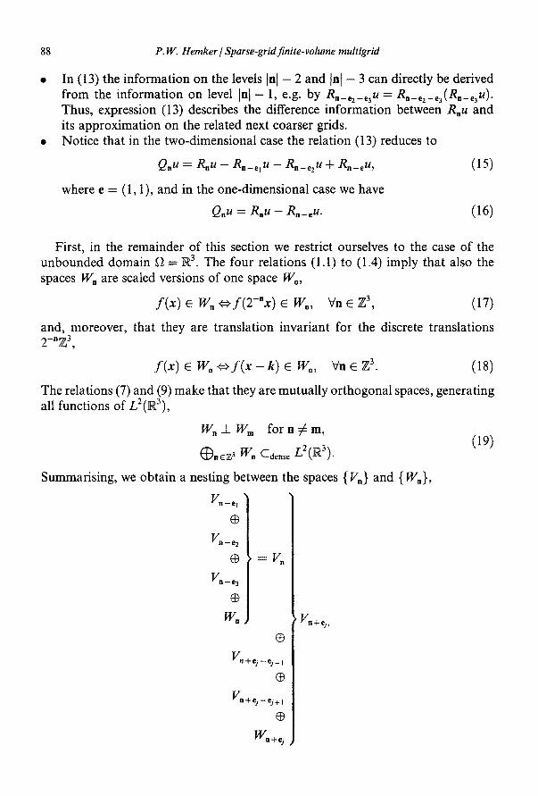
In (13) the information on the levels In[ - 2 and In[ - 3 can directly be derived from the information on level Inl - 1, e.g. by R._e2_e3u = R._e2_e3(R._~u ). Thus, expression (13) describes the difference information between R.u and its approximation on the related next coarser grids. Notice that in the two-dimensional case the relation (13) reduces to

Q.u = R,~u - R . _ ~ u - R,,_~2u + Rn_eU , (15)

where e = (1, 1), and in the one-dimensional case we have

Q.u = R.u - R._eu. (16)

First, in the remainder of this section we restrict ourselves to the case of the unbounded domain f~ = R3. The four relations (1.1) to (1.4) imply that also the spaces W n are scaled versions of one space Wo,

f ( x ) E W. ¢*f(2-*x) E Wo, Vn E Z 3, (17)

and, moreover, that they are translation invariant for the discrete translations 2-nz 3,

f ( X ) E W o e * f ( x - k ) E Wo, V n E Z 3. (18)

The relations (7) and (9) make that they are mutually orthogonal spaces, generating all functions of L2(II~3),

W._t_ W., f o r n C m ,

~nEZ3 W° Cdens e L2(]~3). (19)

Summarising, we obtain a nesting between the spaces { V°} and { IV.},

Vn-e| @

Wn-e • =V~

VII-- e 3 G

w. Wn+ej ' @

g n + ej - ej _ ~

@

Vn+e/-e/+l @

Wo+¢j

P. W. Hemker / Sparse-grid finite-volume multigrid 89

that is essentially more complex than in the classical one-dimensional case, where there is a sequential ordering of the spaces { V.} and { IV.}.

As soon as we find a function ~b(x) with the proper ty that ~b(x - k), k E Z 3, is a basis of W,, then by a simple rescaling, we see that ~b(2"x- k) yields a basis of W~+,. Such a function is the more-dimensional generalisation of a wavelet. Since L2(N 3) is the direct sum of these W~+~, the full collection {~b~,+e(x)[~b~,+e(x)= ~(2nx - k), n, k E Z 3} is a basis of L2(R3).

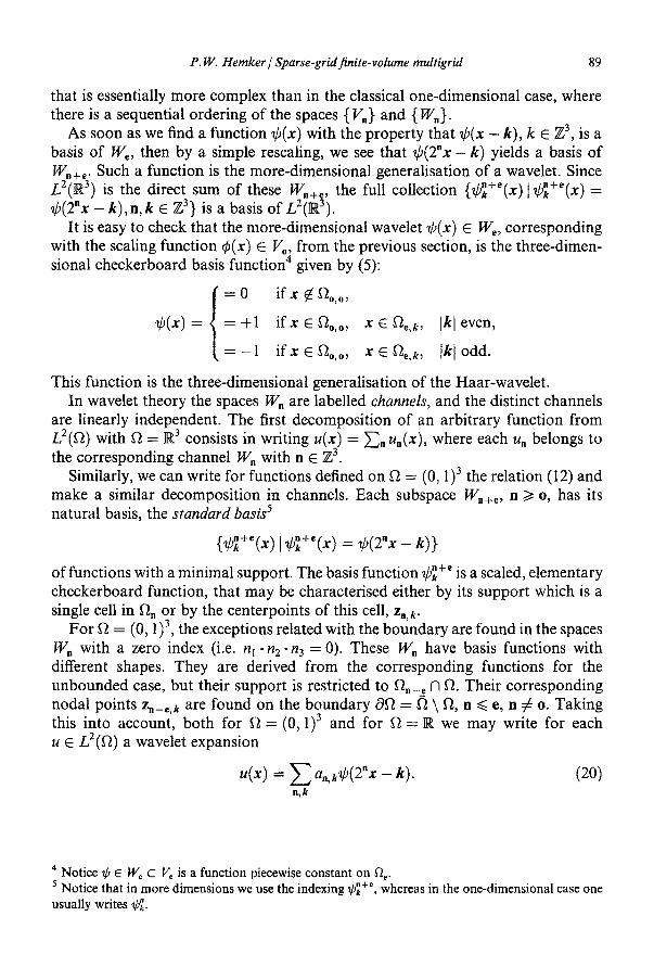
It is easy to check that the more-dimensional wavelet ~b(x) E We, corresponding with the scaling funct ion 4~(x) E V., f rom the previous section, is the three-dimensional checkerboard basis funct ion 4 given by (5):

= 0 i f x ~ f~o,o,

~b(x) = +1 i f x ~ S2o, o, x ~ f~,k, Ikl even,

- 1 i f x ~ f~o,o, x ~ f~,k, Iki odd.

This funct ion is the three-dimensional generalisation of the Haar-wavelet. In wavelet theory the spaces W. are labelled channels, and the distinct channels

are linearly independent . The first decomposi t ion of an arbitrary funct ion f rom L2(f~) with ~ = R 3 consists in writing u(x) = }-'~. u.(x), where each u. belongs to the corresponding channel W. with n c Z 3.

Similarly, we can write for functions defined on f~ = (0, 1) 3 the relation (12) and make a similar decomposi t ion in channels. Each subspace W~+e, n /> o, has its natural basis, the standard basis 5

{~b~,+e(x) 1 ~b~,+'(x) = g,(2"x - k)}

of functions with a minimal support . The basis function ~b~, +e is a scaled, elementary checkerboard function, that may be characterised either by its suppor t which is a single cell in f~. or by the centerpoints of this cell, zn, k.

For f~ = (0, 1 )3, the exceptions related with the boundary are found in the spaces W. with a zero index (i.e. nl.n2"n3 = 0). These IV. have basis functions with different shapes. They are derived f rom the corresponding functions for the u n b o u n d e d case, but their suppor t is restricted to f in- , M ft. Their corresponding nodal points z._ e,k are found on the boundary 0f~ = (~ \ 9t, n ~< e, n ¢ o. Taking this into account, bo th for f~ = (0, 1) 3 and for f~ = R we may write for each u E L2(f2) a wavelet expansion

u(x) = Z a,,,kg,(2"x - k). (20) n,k

4 Notice ~b E We c V, is a function piecewise constant on fl,. 5 Notice that in more dimensions we use the indexing ~b~, +e, whereas in the one-dimensional case one usually writes ~b~..

90 P.W. Hemker / Sparse-grid finite-volume multigrid

2.4. Approximation results

The decomposi t ions (10) or (12) clearly allow the approximat ion of a sufficiently smooth function in L2(ft) by a series with elements in I,V i. To obtain an impression of the quality of these expansions we derive some error estimates.

As the case where boundaries are present is the more general one, we take f~ = (0, 1) 3. To quantify the error of approximat ion on f~, we introduce for U E C3(~='~) t he seminorm 6

tut = sup 03u(x) x~a OXlOX2OX3

Now we derive the following

]( 0 ; ( 0 ) q ( 0 ) r • + max sup ~ - - - - u(x)

P,q,r=O, l xsOft COX 1 OX 2 COX 3 (21)

Theorem 2.2 If we consider an expansion o f a C3(~)-funct ion, u, in piecewise constant functions on the grid ~in, for an arbitrary n E Z 3, n > o, and if we write

R.u = vo + ~ ui, o~j~<n

w i t h y oC V o a n d u i E W i, o <~ j <~ n, then

IlujllL:(n) ~< 2-3ul/21ul,

and we get an estimate for the approximat ion error

[lu - Rnullf2(n ) ~< 8.7-3/2(2 -3'' + 2 -3"2 + 2-3n3)l/2[u I

<.N 8.7-3/2(h3/2 + h~/2 + h~/2)lul. (22)

Proof We take the normalised {~)/} = {21J-~l/2~p~} as a basis in Wj, o ~<j~< n, j C o . Clearly, all those functions are or thogonal to all functions Vo c Vo and mutual ly they form an o r thonormal set (an o r thonormal Haar basis) in W i c L2(f2). We see this as follows

~ W e ,

We,

we,

suppor t (~b) = f~o,o,

support (~b~,) --- f2o, k,

suppor t (~b~) = f2i_e,k,

(23)

or, in other words, ~b~ E V i, but ~L scales like a basis funct ion in V~_ e. Hence

/ 91j-el/2d,jglj-el/2d,j df~ 0 for k # m~ Wk ~ wm

6 The necessity of the boundary terms in this seminorm is seen immediately if we want to approximate in L2(f~) smooth functions u E C3(~) that do not satisfy homogeneous boundary conditions.


and

f "~li-el/Z°d'~lJ-~l/2"/"i df't = 21i-~t f "~]~] dUt = 21J-°l fa vk'- +k -o,k df~ = 1.

Thus, we find R.U = Vo + ~ uj,

o~<j~<n with

uj = ~ ajk(bd = y~(u, (bd)(b~. k k

Now

aj. ( u , ~ d ) ~ u ~ b L d f ~ fa, -J = = = u ~ k dO. -e,k

By Taylor expansion around Zj_e,k, we have

a~_o,k u@d df~ ~< 2-21Jt)t i. (24)

F o r j I> e the point zy-e,k lies in the interior of f~ and the estimate holds with

lu l=sup 03 u(x) ] x~f~ OXlOX2OX3 ."

For j ;$ e, i.e. for ~b~ with .bcomponent equal to zero, the point zj_e,k lies on the boundary and the function ~b~ is constant in one direction over the whole domain f~, and it is of Haar-wavelet type for the non-zero indices (or index). In this situation the same estimate (24) holds with, e.g. if j l = 0,

1 02u(x) 1 lul = sup ~ l '

For j = o the relation (24) is trivially satisfied. Hence, the estimate (24) holds for j I> o if we use the serminorm (21), and we find

la, kl ~ 2-2Lyllul,

so that

and

llujll: = ~ lajkl 2 ~ ~ 2-arJtlul 2 = 2-slJllul 2, k k

Ilujll ~ 2-31jl/2[ul,

l l u - R.ull: = Jl >n! nl Jl >~ 0 Jl >/0

orj2 >n2 Z,>n2 j_, I>0 °r J3 > n3 J3 >/0 J3 > n3

92 P. W. Hemker / Sparse-grid finite-volume multigrid

~< (~ )3 (2 -3" l+2-3n2+2-3n3) lU]2 .

and it follows that

llu - Roull <. (2 -3nd2 + 2-3nd2 + lul

= (~)3/2(h3,/2 + h~/2 + h32/2) lu,. []

I f we have no further a-priori knowledge about u, the most efficient approximat ion will be one with h~ = h2 = h3 because this equalises the three main terms in the error bound. We see that

Rn=~-~Qj, j <<.n

and the t runcat ion error for u - Rnu is neither particularly promising nor surprising: the major part of the error is produced by the largest meshwidth: (max(hl,h2, h3)) 3/2, whereas the total number of degrees of f reedom for an element in V. is 2 Inl.

Following the idea of sparse grids, as in t roduced for finite elements in [3,9], a better accuracy per degree of f reedom is obtained for the approximat ion operator

dl~m = ~ Qj (25) lJl ~< m

with m E Z.

Theorem 2.3 For the approximat ion operator (25) we have the t runcat ion error estimate

liu - Rmu[[ < M(e)R-(3-~)m/2]u I = M(e)(hlh2h3)I3-')/2lu 1. (26)

for some arbitrary small constant e and a constant M(e), depending on e.

Proof Following the same lines as in theorem 2.2, and because ]]ujl ]2 ~< 2-3ijl ]u], we get

I lu - Rmull 2= ~ Ilujll = Ijl>m

~< lu] 2 ~ 2 -3u I= lul 2 ~ ~ 2 -31jl

IJl >m l>m lJl =1

= l u 1 2 ~ ( / + 1)(1 + 2) 2_a2_i3_,) , 2 l> rn


Hence

lul2M(E) 2 2 -O-')t l>m

= lu12M(e)22-mO-'). (27)

Ilu- kmull ~< M(c)2-m{3-')/2{ut, (28) where 2-" = h~h2h3 is the volume of the smallest cells in the sparse grid used for the approximation of u. []

In (22), all hj need to be small and in (26) only their product. This means that for convergence in (22) all meshsizes should tend to zero, whereas in (26) only the area should vanish. Further, the estimate (26) is of the same order of accuracy as (22), except for a logarithmic small factor. However, the number of degrees of freedom for the approximation (26) is significantly less. Namely, in the unit cube, for R.u the number of degrees of freedom is 2 Inl, whereas for /~mu it is (m 2 + m + 2)2 m - 1. Because significantly fewer degrees of freedom are involved in the approximation Rmu than in the approximation of R(m,m,m)12, i.e. fewer coeffi- cients aj, k and fewer gridpoints zi, k, following [3], we call the approximation Rmu the sparse grid approximation and

f2~,= {zj, k I zj, k E f~;, [jl ~<m}

is the sparse grid or sparse box grid for this approximation on level m. In this paper we are interested in the approximate solution of PDEs discretised

on a sparse grid, i.e. we are looking for an approximation of the solution of these equations in the space

in I ~< m InI ~< m

or, for f~ = (0, 1) 3, in the space

= • v, = ro • o .< Int --<. m

We call S,,(f~) the mth level sparse-grid space.

O w.. o~<lnl~<m

3. The multigrid algorithm

The basis principle of multigrid for the solution of the discrete equation

Lhuh = fh

is that the high frequencies in the error are reduced by relaxation on a fine grid, whereas the low frequencies are taken care of by coarse-grid discrete equations.


The classical coarse grid correction (CGC) step is described by

u (new) = u (°l°) + PhHLZ, l Rm, (fh - LhU(°ld)),

where LH is the coarse-grid discrete operator and Phn and Rm, are the grid-transfer operators f rom the coarse-to-the-fine and fine-to-the-coarse grid respectively. Uusually the coarse-grid mesh size is twice the mesh size on the next finer grid. The coarse grid problem is approximately solved by means of the recursive application of the same algori thm on the coarser level. In this classical procedure a linearly ordered sequence of fine and coarse discretisations is required.

In the case of our sparse-grid finite-volume approximat ion, a discretisation should exist for all grids f~., In] ~< m, fine and coarse. On each of these grids we can obtain approximat ions to un E V~, the solution of the discrete problem

L.u, =fn on ~ , . (29)

These discretisations, however, do not offer an ordered sequence. Nevertheless, the mult idimensional wavelet decomposi t ion of ua EVa,

ua = Vo + ~[] 1~/, with wj C W~, j~<n

allows us to distinguish a high-frequency component , wa, that cannot be represented on coarser grids, and all other components , vo and wj, j ~< n, j ¢ n, which can be present in coarser grid representations. Therefore we may consider the grid ~ . to be solely responsible for the accurate (and efficient) representation of w,. This componen t is clearly a high-frequency function (in fact a checkerboard- type function), of which an error can be efficiently reduced by a simple relaxation procedure as e.g. damped Jacobi.

The decomposi t ion (13) in theorem 2. I shows us how a CGC can be obtained from these coarser grids in ~2,_ej, J = 1,2, 3,

u(new) . (old) n =Un -}" Z Pn'n-ejLn!ejRn-e) 'nl'n

j = 1,2,3

- - Z Pn.n-e+ejLNle+eJRn-e+% hr. j = 1,2,3

with

+ P a n eLn fern earn , (30)

(old) r~ = f ~ - L ~ . ~ . (3t)

Here we denote by Rm, n: V, ~ V m, m ~< n, the restriction operator defined by Rm, nU. = Rmu,, for all u~ E V. c L2(f~). The prolongat ion opera tor P.,m: Vm--' V. can be defined e.g. as the adjoint of Rm,..

The third remark following theorem 2.1 shows how the two- or one-dimensional case can be treated similarly and we see that - for the one-dimensional case - our approach reduces to the classical scheme.


1 cn-e+ei = 2 (R"-~+%"-e~+~c"-~j+l + Rn-e+%n-e~_lc,-ej_~),

j = 1,2,3, and 1

c . _ , = 5 ./=1,2,3

This is justified by the fact that the restrictions are commutat ive, i.e.

m <~ n <~ ! ~ Rm, nRn, t = Rm, t

and the following (trivial) lemma.

The approach (30) would imply three coarser levels to be active for a CGC, and - as was shown in the remark after theorem 2.1 - we can do with only one coarser level by deriving the informat ion on the levels tnl - 3 and Inl - 2 f rom the informat ion on level Inl - 1. If we consider the corrections f rom level Inl - 1,

Cn_ej = L-~l_ejRn_ejRn_ej,nrn, j = 1,2, 3, (32)

as approximat ing a single (but unknown) correction function c. E V., the corrections f rom the levels In I - 2 and lnl - 3 can be computed as the mean values

(33)

Lemma 3.1 If all discrete operators Ln are stable and relatively consistent, i.e.

IIR.,.+ejL.+o~ - L .R. , .+~II <~ O(2-I"IP),

then

lic.-~j - R . _ % . c . l l < O(2-1"IP).

(34)

The consistent discretisations can be derived e.g. f rom the fine grid discretisation L. by taking the Galerkin approximat ion

Ln_~j = Rn_ej,.LnP.,n_ej.

If the three corrections c._,j were all restrictions of the (unknown) correction c. E V. indeed, then Rn_e+ehn_ej+,Cn_ey+l and Rn-~+eg,"-~9-' c._~9_, would both have delivered the same result, viz., R._~+~j,.c.. This gives the possibility to check how well such a function Cn can be determined, by moni tor ing the quantities, j = 1,2,3,

1 d._e+ej = ~ (Rn_e+ehn_ej+,Cn_ej+1 -- Rn_e+ej ,n_ej_,en_ej_, ). (35)

Summarising, our mult igrid a lgori thm now reads:

(i+ 1) = u(ni) un + j=1,2,3

j= 1,2,3

-I- Pn, n_eCn, n_e,

Pn, n-ej cn-ej

Pn, n-e+ejCn-e+ej

(36)


where the corrections are given by (32), (33) and (34). This appears to be much similar to a multigrid algorithm by semi-coarsening, proposed by Mulder in [7]. The main difference being that Mulder computes an approximation on the full grid Rn, whereas we compute the sparse grid approximation Rm.

The result of our algorithm is a solution on a sparse grid, i.e. a set of approximate solutions, viz. {u.] In] = m}, that are the solutions of the discrete equations Lnu, = f . . All approximations u, representing the same solution u of the continuous problem, we assume that they approximate the LZ(f~)-projection of u in V m = V(m,m,m ). To approximate this Rmu C I'm, we can construct a unique function Um E Vm by means of the recursive interpolation formula that immediately follows from theorem 2.1:

uk = Z (uk_~j - uk-e+~j) + Uk_~, (37) j=1,2,3

where o ~< k ~< m, tkl = m + 1 , . . . , 3m; uk_ej are the functions computed in the previous recursion cycle and Uk_e+ej and Uk-e are approximations (possibly) derived as (33) and (34). In this way we finally obtain the unique representation

Um=Vo+ Z wk (38) o .<< Ikt -< m

o r

• s (a) c

This representation can be considered as the computed solution. The same construction can be realised by a "decomposition and reconstruction"

algorithm as used in wavelet theory [2]. Then the available approximate solutions {u,} are decomposed into their components % and {wk} by

Inl=~ InJ=m Vo - and w k --

521 Int =m Inl =m

and the reconstruction is performed by (38). This can conveniently be performed by a kind of a "pyramid algorithm". This will be reported in a later paper.

In practice, by the choice of the discrete operator our assumption that the L2(f2)- projection of u was indeed consistently approximated on V,, may not necessarily hold, and it can be checked by a monitor as (35). Now, e.g. the corresponding erroneous components might be removed from the sum (38).

In the light of the treatment in section 2 it is clear what restrictions and prolongations can be used between the different grids in the multigrid process. Because Vn C L2(f~), the obvious restriction R._ej,, is the L2(ft)-projection onto Vn-ej:

R n - % n = Rn-e i .

P. w. Hemker / Sparse-grid finite-volume multigrid 97

This makes the diagram for the restrictions commutative: for any ! ~< m ~< n we have Rl, mRm, n = RI, n.

An obvious prolongation can be the transposed restriction

T P~,n-ej = R~-ej,n.

However, this prolongation being of low order, it may be more appropriate to consider higher order prolongations. Such prolongations can always be represented by an additional operator B.: II. ~ V. so that we have

Pn, . -e j = B .Rr . -e j •

Here we will not elaborate on the different possibilities for B,. The algorithm (36) shows that all relaxation processes for u. on one and the same

level m = lnl can be made in parallel. The cycling between the different (scalar) levels can be made as for the classical multigrid method: we can distinguish between V-, W- or F-cycles. However, in order to prove that the convergence of our multigrid-method is independent of the meshwidth, we now have to take into account that all aspect ratios will appear in the discretisations used.

4. F o u r i e r convergence analysis

In this section we first summarise some results of Fourier analysis for more- dimensional discrete approximations and then we apply this to compute the convergence rate of our sparse-grid multiple-grid methods for the solution of the anisotropic Poisson equation. The approach is different from the usual treatment of Fourier analysis for multigrid for finite difference methods for the following reasons. First, in view of the discretisation of conservation laws and divergence problems, we study nested box grids. This implies that mesh points in the coarse grids do not appear in the fine grids as well. The nesting of the (box) grids is different from the usual nesting of the (finite difference or finite element) grids. Second, we do not consider the usual sequences of fine and coarser meshes for multigrid methods, but we allow d-dimensional (d = 2, 3) sparse grids.

Fourier analysis is one of the common tools to analyse linear constant coefficient problems on regular grids, and it is particularly useful if the treatment of boundary conditions can be neglected.

In section 4.1 we describe general tools that can be used for the Fourier analysis of functions defined on more-dimensional box grids. The definitions and theorems provide a useful machinery for the application of local mode analysis for the multigrid box-methods. For the technical proof and details related to this section we refer to [4].

In section 4.2 we apply tools to analyse the multigrid algorithm introduced in section 3. The technical preparations in section 4.1 allow us to be brief and clear in this treatment.

9 8 P. IV. Hemker / Sparse-grid finite-volume multigrid

4.1. Fourier analysis for sparse box grids

For u E Lz(R 3) we introduce its Fourier Transform (FT) fi, scaled as

fi(w) = (27r) 3/2 . ~ e-iX~'u(x) dx. (39)

Then we know that fi E L2(~3), and a back-transformation formula is available,

t~(x) = (27r) -3/2 : e+;X~'fi(w) dw, (40) JR 3

such that f i (x)= u(x) almost everywhere on IR 3. Moreover, fi ~ L2(IR 3) and Parseval's equality holds: I lulIL2(R2) = I lfillL2(R3).

We are interested in the Fourier transformation for an infinite set of equally spaced data. In this case the FT of such a "grid function" is a periodic function (a function defined on a torus). Therefore we introduce a few definitions.

Let h E 1t~ 3, h > o, be given, then the h-periodisation of a function u: ~3 ---, C is defined by

f i (x)= ~ u(x -kh ) , (41) k E Z 3

where kh=(klhl,k2h2,k3h3). We also introduce a notation for the three- dimensional torus

Th = (-Tr/h, 7r/hi = (-Tr/hl, 7r/hl] × . . . × (-Tr/h3, 7r/h3]. (42)

Further, we need the functions 17 and Sinc [1, pp. 62, 67] on ~3,

1 f o r l x i l < l / 2 , 1~<i~<3, II(x) = (43)

0 otherwise,

and

sin 7rxi S i n c x = ? ~ ~ .

Using the relations mentioned in [1, p. 98] we find

0./ HI /= I/sinc(; ) /441 i = 1 , 2 , 3

For an h 6 N 3, h > o, we define the dilation operator Dn: L2(]~ 3) --+ L2(]~ 3) by

Dhf(x) = h-V2f(xh), (45)

where h = (hlh2h3) 1/3, and the convolution operator,., by

( f . g)(x) = (27r)-3/2 JR/3 f (y )g(x - y ) d y . (46)

P. w. Hemker / Sparse-grid finite-volume multigrid

We now know that

= D1/hf and f . " g ( w ) = f ( w ) . ~ ( w ) .

99

(47)

4.1.1. Grid functions Here we introduce notations for the different types of grids and grid functions.

Definition 4.1 For a fixed mesh parameter h E ~3, h > O, and f o r j E 7Z3, we define an elementary cell by f2h, j = {xl jh < x < ( j + e ) h } , the volume of the cell is denoted by h 3 = hi "ha "h3, and the box-grid is defined by [2h = {f~h,j [J E Z3}. The regular infinite three-dimensional grid of vertices Zh is defined by Zh = {jh IJ ~ Z3}, which should be well distinguished from the shifted grid which is defined by g~ = { ( j + e/2)h IJ ~ Z3} •

Notice the relation with the grids as defined in section 2.2: f~n can be considered as a special case of f~h, and f~ as a special case of Z~.

Definition 4.2 A complex or a real grid function u'h is a mapping Zh ~ C, or Zh ~ R, and a shifted or box-grid function u*h is a mapping Z~, ~ C or Z~ ~ R.

The vector space of such grid functions we denote by l(Zh) or I(Z;), or briefly, by l. For any p >/ 1 the space l(Zh) can be provided with a norm I1" lip

IMllp = h 3 lu'h(jh)l p (48)

For a fixed p, all grid functions with a finite norm 11. lip form a Banach space denoted by lP(Zh). For p = 2 we know that 12(Zh) is a Hilbert space with the inner product

(u~, v*h)t2(z,) = h 3 ~ u'n(jh)~(jh) with u], v~, E Zh. (49) j~Z 3

Similar definitions are given for I(Z~,):

* * = E Uh(Z)Vh(Z) with Uh, Vh E Zh. h 3 * = * * * ( 5 0 )

zEZ~

Definition 4.3 The direct restriction R'h: L2(]~ 3) ~ l(Zh) is the operator that associates with a continuous 7 u E L2(R 3) the corresponding grid function on the grid Zh, defined

7 In case of a discontinuous function we can replace u by ~ as defined in (40).

1 O0 P.W. Hemker / Sparse-gridfinite-volume multigrid

by (R'hu)(jh) = u(jh), Vj C Z 3, (51)

and the direct restriction R'n: L2(I~ 3) ~/(Z]~) on the shifted grid Z], is defined by

(R*nu)((j+ e/2)h) = u((j+ e/2)h), Vj e Z 3. (52)

Definition 4.4 The box restriction Rh: Lz(N 3) - - * L2(~ 3) is the LZ-projection on the piecewise constant functions on f~h, defined by (cf. equation (6))

(Rhu)(x) = h -3 [ u(z) dz, Vx (53) dst

The box-restriction RSn: L2(]~ 3) --' l(Z;t) is defined by Rg = RnRn,* • it associates the mean value of u on a cell f~,i with the nodal value at the centre of ~2n, i.

The box-restriction Rgu should be well distinguished from R*nu. However, the L2(fl)-projection Rnu in (53) and the restriction Rgu in (52) are conveniently related to each other by

Rhu = R*h((DnII) * u). (54)

4.1.2. The Fourier transform of a grid function Let u;,: Zh ~ C be a grid function. We give the following

Definition 4.5 L2(Th) of grid function u~ c 12(Zh) is a function The Fourier transform u h E a

Th ~ (2, defined by

/ ]7 NI3~"~ -ijh . . . . . . ~(w) = t ~ ! 2 ~ e uh(jn ). (55)

\x/27rJ iez3

The inverse transformation is given by

( I ) 3 f ~ e+"n'~(w) dw. (56)

Let u~,: Z] ~ C be a shifted grid function, then we have

Definition 4.6 The Fourier transform u~ E L2(Th) of a shifted grid function u~ E 12(Z~) is a function T h --~ C, defined by

~ ( w ) = ~ e-i(J+e/2)~°u;((j+e/2)h). (57)

P.W. Hemker / Sparse-grid finite-volume multigrid

Its inverse t ransformat ion is given by

u ; ( ( j + e/2)h) = e+ilJ+'/2)t"'~(w) dw. ~rh

101

(58)

Remarks

We immedia t e ly see that ~ (w) is [27r/h]-periodic, whereas t ~ ( w ) i s [27r/h]- antiperiodic, i.e. u*h(w + 27r/h) = (-)lelu],(w).

• We denote the Fourier t ransforms also by

u h = )V(u~) or Uh = ~'(Uh), (59)

i.e. we introduce the mapping ~ : /2 (Zh) ~ L2(Th) or f : 12(Z],) ~ L2(Th). At the end of this section we shall generalise this meaning of .T'.

• By the Parseval equality we have

Ilu;l12 = IluhllL (Th) and Ilugl12 -- Ilu, llL It,). (60)

Hence the Fourier t ransformat ion operators Yr:12(Zh)~L2(Th ) and 5r: 12(g]t) ~ L2(Th) are unitary operators.

* f ~lekle* • Because e~,.,, = e~,.,,+2~,/, or e,.~, = ~- / ,.,o+2~k/,, for all k E 7/"3, on a mesh of size h a frequency w cannot be distinguished f rom a frequency w + 27rk/h. This phenomenon is called aliasing.

4.1.3. The relation between FTs of a function restricted to different grids In this section we first present a few theorems associated with the different

restrictions between two grids. We describe the relation between the FT of a con- t inuous function defined on N 3 and the F T of its restriction to the grid and then we show the relation between the FT of a fine grid function and the FT of its representation on a coarser grid. Next, we give the corresponding theorems for the prolongations.

Lemma 4.7 Let u E L2(~ 3) be a cont inuous function with FT ~. Its restriction u.~ to the grid gh is defined by (51). We have the following relation between h and u~,:

~(w) = ~ ft(w+ 27rk/h), (61) k E Z 3

is the [2rr/h]-periodisation of ft. i.e. u h

Proof For the p roo f we refer to [4]. []

In the following lemmas q-restrictions are considered, with q E Z 3. Here q = (ql, q2, q3) is the coarsening factor, where usually 1 ~< qy ~< 2, j = 1,2, 3.

102 P. W. Hemker / Sparse-grid finite-volume multigrid

Definition 4.8 Let q E Z 3 with q > o and H = qh, then the canonical q-restriction P~ is the operator Rq: l(Zh) ~ l(Zqh) = t(Zn), defined by

( R;u'h) ( jH ) = u~(jH ) = u'h(jqh ). (62)

Theorem 4.9 We have the following relation between the FT of a grid function and that of its canonical q-restriction,

(R~u'h)(w) = ~ ~(oa + 2Top~h), Voa e Tn, H = qh. (63) ,e[o,q)

Proof For the proof we refer to [4]. []

Lemma 4.9 shows that, using the restriction R~ with q C Z 3, q > o, we get aliasing of q3 = q~ "q2"q3 frequencies onto one.

Now we describe the relation between the Fourier transforms of a continuous function and its box restrictions. First we consider the direct restriction to the shifted grid, R~, and later the box-restriction, Rh and the q-restriction Rq.

Lemma 4.10

= = + 2 k/h).

k E Z 3

Proof For the proof we refer to [4].

For the Fourier transform of u E L2(II~ 3) and Rhu E L2(~ 3) following relation.

(64)

[]

we have the

Theorem 4.11

~(w) = R .u (w)= ~ (_);kl Sinc ~ + k .a(w + 2rck/h). k E Z 3

Proof Using (54) we see

=

= - - .F'(R**,((DhlI) * u))(w)

k

(65)


k

= (2-~)3 /2Z(- ) lk lDl /h~(oo-k-2rrk /h) .~(6o+2rrk /h ), k

Z (w : k/h).fi(w + 2rrk/h). = h -3/2 (-)lktD~/h Sinc k

) = Z ( - ) It'I Sinc ~-~+ k .gt(w + 2rck/h). (66) k

[]

Definition 4.12 Let q E Z 3 with q > o and H = qh, then, for s E [o, q), the s-frequency decomposi-

s. l(Zh) ~ / (Z qh ) = I(Zn) is defined by tion q-restriction is the operator Rq.

(l~qu*n)((j+e/2)t-I)=q -3 ~ (-)St'u*h((qj+k+e/2)h), (67) k~[o,q)

w h e r e q3 denotes q3 = ql "q2" q3.

Remarks 0 ¢¢ • In the case s = o we call/~q = Rq = Rq simply the q-restriction.

• F r o m the construct ion of the restriction operators Rn s a n d / ~ it is clear that the following relation holds:

R ~ . B = RqRh.

Theorem 4.13 Let q = 2e E Z 3, then for all w E T 3, H = 2h, we have

(Rquh)(w)=2q_3i s ~_~ (_ )mCo s h w + ~ r ( m + s ) . . ~ ( w + ~ / h ) , me[o,q) 2

where

Cos(hw/2)= H cos(hjwJ2). j= 1,2,3

Proof For the p roo f we refer to [4].

Definition 4.14 The natural box-prolongation P'h: 12(Zh) ~ L2(]I~3) is defined by

u(x) = (/~DZ)(x) = uh((m + e /2 )h) ,

(68)

[]


for all m C Z 3 and mh < x < (m + e)h. We also introduce a natural prolongation, * • • * 2 * * P~, from a coarse to a fine grldfunctlon P~: l (Zn) --~ 12(Zh) by P~ = R ~ where

• * 2 3 - H = qh. The prolonganon P~h: l(Zh) -~ L ( R ) is the operator dual to R~ in the sense that for all u~, E lZ(Z~,) and v E L2(R 3) we have

( P~ u~, v) t.2(~3) = (u;,, R~ v),2(z~). ( 69 )

The following theorems show how we find the FT of the prolongation if the FT of the source function is given.

Lemma 4.15

a(to) = f(P u )(to) -

Sin(hto/2) ~(to)• (70) hto/2


Theorem 4.16 With H = qh and q3 = q~. q2" q3, we have for the FT of the prolongation of a box gridfunction

q-3 Sin(Hto/2) A ~(w) = Y:(P*qu*n)(w)= Sin(hto/2) u*n(to). (71)


4.1.4. The Fourier transform of operators involving different grids In (68) and (71) we see that, by the restriction and prolongation between func-

tions on grids 9t n and ft.+q, aliasing takes place and that q3 frequencies on f~,+q correspond with a single frequency on f~.. This implies that, analysing a multigrid algorithm, we have to study the behaviour of the q3 aliasing frequencies together. Collecting the q3 corresponding amplitudes of the aliasing frequencies in a single q3_ vector, we extend the definition (59) of.T to the case q3 > 1 and obtain ~': 12(Zn) ---, [L2(Tqh)] q3 o r ~-: lZ(z]) ~ [L2(Tqh)] q3 by

ffY(Uh)(t.O ) ~-- (~lh(to --~ 71"lll/h))mE[o,q), O.1 E Tqh. ( 7 2 )

With these amplitude-vectors .T(u])(w) and .T(u])(w), we can introduce the linear operators .T(R'q)(W) and JC(R*q)(w) by

.T(R;u'h)(to) = Yr(R'q)(to).T(u'h)(to), to C T,h, (73)

and

~(R*qu*n)(to) = ~(R*q)(to).f(u*n)(to), to C Tqn. (74)

We call the new operators, that depend on to, the Fourier transforms of the original

P.W. Hemker / Sparse-grid finite-votume muttigrid 105

operators. The new operators are g x q3g matrices if g aliasing frequencies are considered on the coarse grid.

Similar to the restrictions, the prolongations can be associated with their Fourier transforms.

and

.~(P;u'h)(w) = .~(P'q)(W)~(u'h)(w), w E Tqh, (75)

U(P*qu*h)(w) = Y~(P*q)(W),T(u*h)(w), w E Tqh, (76)

These operators are q3g x g matrices. For arbitrary linear constant coefficient operators Ah: 12(Zh)~/Z(Zh), its

Fourier transform ¢'(Ah): LZ(Tn) ~ L2(Tn), can also be considered as a q3g x q3g diagonal matrix

7(Ahuh)( o) = V,, Tqh.

Because of Parseval's equality we know that

[[Ah[[2 = max [[Sr(Ah)(w)[[2 = max o(.Y'(Ah))(w), (77) ~GTqA WETqh

with o-(A) the spectral norm (the largest singular value) of the matrix A, and

p(Ah) = max p(U(Ah))(w) , (78) w E Tq~

where p denotes the spectral radius. This provides us with the means to study the norm and the spectral radius of the error-amplification operator of the multigrid iteration.

4.2. Fourier analysis convergence results

To get some insight in the behaviour of the more-dimensional multigrid algorithm introduced in section 3, we use the Fourier analysis to determine the convergence rate of the two-level algorithm for the two-dimensional anisotropic Poisson equation

Uxx -[- ~2 Uyy = f , (79)

discretised by the usual 5-point discretisation. The error-amplification operator, Mr., of the two-level cycle (with/z pre- and u

post-relaxation steps) for the solution of (29) is described by

e(i+l) = Mne~i) . ~ ( ' .~p(i) (80)

where Sn denotes the smoothing, e.g. damped Jacobi iteration:

(new) She(Old) (In aD; 'L . ) e~ °ld), (81) e n ~ ~ _

with a the damping parameter and D. the main diagonal of the discrete operator L.. The coarse grid correction is described by (30) and (31). For gridfunctions


u, E 12(Z~), i.e. neglecting boundary conditions, we find, using (30)

:r(M.)(,,) = J:(Sn)~(~)J:(C.)(~,)J:(S.)"(~), with

and

~-(s.) = ~(I .) - c~'(O.)-l~(L.) ,

(82)

(83)

and

/ t~lhl cos )V(R.-e 2 .) = [

' \ 0

J:(R._,,.)= (

0 sin w2h 2 0 ~ ,

) COS w2h 2 0 sin w2h 2

sinwlhl 0 0

) 0 coswlh2 sinwjhl

cos(~l hi ) cos(~2h2) , T sin(wlhl) cos(w2h2) ]

cos(wlhl) sin(w2h2) / "

sin(wlhl) sin(w2h2) ]

So, with 5v(P. , ._ , , )= U(R._e,,.) r, .T'(Pn, n_e2 ) = U(R._~2,.) r and ~- (P . , . -e )= .~(R._,,.) r, the norm IIMn[I and the spectral radius p(M.) can be computed by means of (77) and (78).

From (68) and (71) we know

.) = ( cosw2h2 .F ( R,_e,

' \ 0

7(C.) = f f f . )

- ~ f(e, , . -oj)~(L.-e)-~7(R.-ej , . )~:(L.) j= 1,2,3

+ ~ 7(~.,.-,+,)~:(L.-o+o)-I~:(R.-o+o~,.)f(L.) j= 1,2,3

- 7(P.,n_,).~(Ln_e)-'.~(R._e,.).~(L.). (84)

To get an impression of the behaviour of the algorithm, keeping the explicit computation to reasonable size, we elaborate (82) for the equation (79), for the two-dimensional case, with q = (2, 2) and ~ = v = 1. Then YZ(M.)(w) is a 4 x 4- matrix, which we derive from (82), (83) and (cf. (15))

~-(c.) = Jr(z.)

_ :r(~. , ._ . , ):~(L._., )-' ~:(R._. , , . )~:(L.)

- :F(P.,._,~.)Y(L._,.)-I.~(R._.2,.)y(L.)

+ Y(P., ._,) .~(L._.)-~.~(R._, , . )Y(L.) .

-o,a

o.6 o.4

o.1

o .o$

o,o$

(a) The eigenvalues of

o.l

o . e ~

t •

(b) The eigenvalues of

.o.o;

*G.o4

a.i

o

(c) The eigenvalues of .T(Mn)(W).


o,J,

*,*s,

0 , s

*,ts

*.*s

(d) The singular values of ~-(Mn)(w).

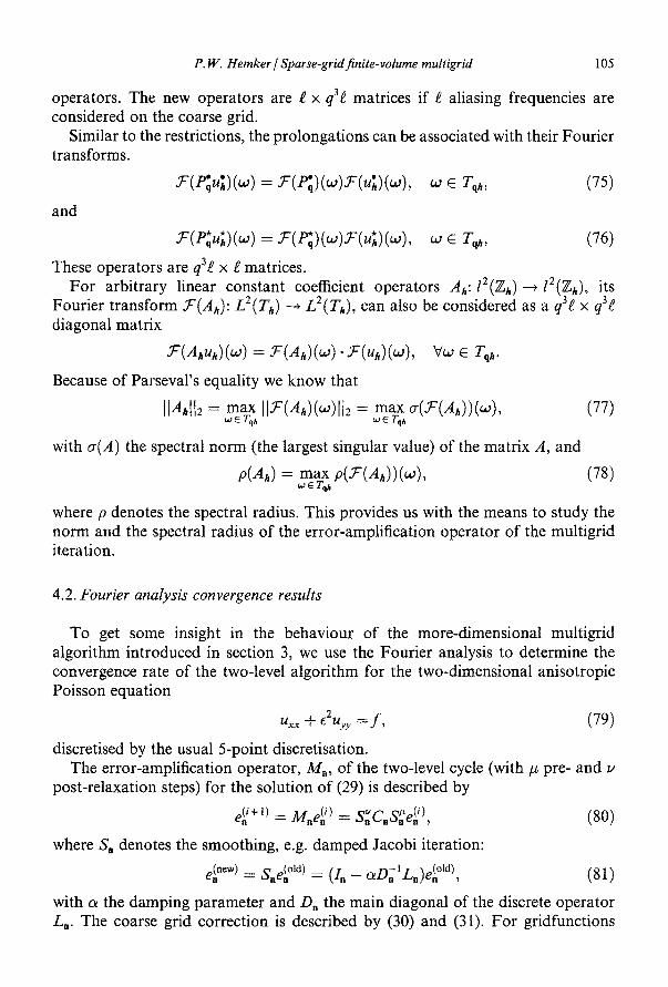
Figure 1. The frequency response of the operators S. , C. a n d Mn, for e = 1, q = (2.2) a n d a = 2 /3 .

To study the convergence behaviour of our algorithm, we consider the matrices (83), (84) and (82) as a function of w E Th = [ - n / h , 7c/h] 2, and for each w we compute the eigenvalues and singular values of these matrices. We show these values in figure 1 for the case a = 2/3 , E = 1. Without loss o f generality we can take h = (1, 1), the parameter e taking care of the anisotropy. The damping parameter a E [0, 1] for the Jacobi relaxation can be chosen freely. We select the value a = 2 /3 because it minimises

max p(~(S.)(w)). " , = (o, ~rl/,), (¢, o), (~/h,,~/#,)

This means that o~ = 2 /3 makes S. a well balanced smoother for the different types of high frequencies (see figure la).

In figure 1 a we show the eigenvalues of the smoothing operator, and in figure lb o f the coarse grid correction. In this figure we see that one eigenvalue of .T(C.) is always equal to one. This eigenvalue corresponds with the highest frequencies, for which no correction can be obtained from any of the three coarser grids. The combined effect of the smoother and the coarse grid correction is seen in figure lc, which shows that sup., p ( M . ( w ) ) ..~ 1/9, and also in figure ld, where we see

108 P.W. Hemker / Sparse-grid finite- volume multigrid

o.I o.+

(a) The eigenvalues of 9V(Mn)(oa).

1.6 l.t

o,1

o++ o.4

(b) The s ingular values of ~'(Mn)(Oa).

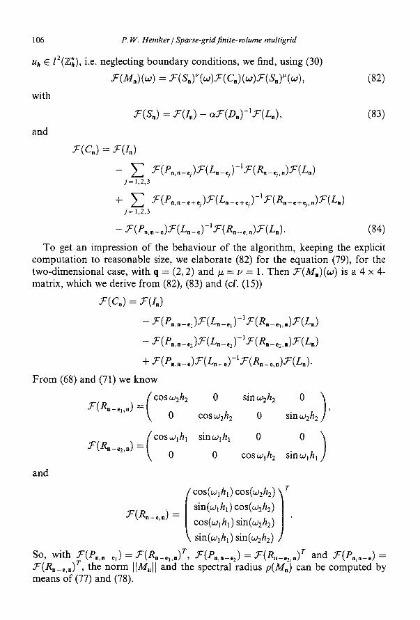
Figure 2. The frequency response of the operator 3//., for e = 1/8, q = (2,2) and a = 2/3,

sup IIM.( )It ~ 1/3. The rather low maximal values show that - at least for square fine-grid cells - the multigrid algorithm has good convergence behaviour.

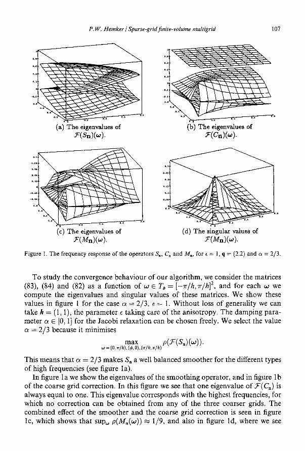
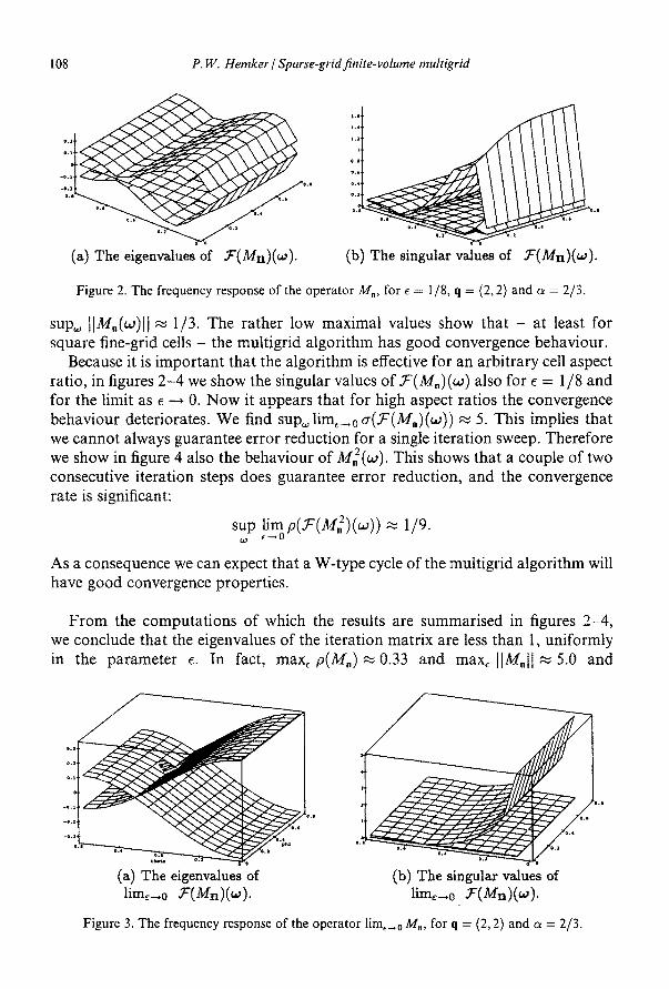
Because it is important that the algorithm is effective for an arbitrary cell aspect ratio, in figures 2 - 4 we show the singular values of 9r(M,)(w) also for e = 1/8 and for the limit as e ~ 0. N o w it appears that for high aspect ratios the convergence behaviour deteriorates. We find sups, lim+~0 cr(Sr(M.)(w)) ,~ 5. This implies that we cannot always guarantee error reduction for a single iteration sweep. Therefore we show in figure 4 also the behaviour of M2.(w). This shows that a couple of two consecutive iteration steps does guarantee error reduction, and the convergence rate is significant:

!im pC.F(M2. )(w)) .~ 1/9. s u p ~ --"p u

As a consequence we can expect that a W-type cycle of the multigrid algorithm will have good convergence properties.

From the computations of which the results are summarised in figures 2-4 , we conclude that the eigenvalues of the iteration matrix are less than 1, uniformly in the parameter e. In fact, max+ p(M.),-~0.33 and max+ IIM.II ~ 5.0 and

.O. -¢.2 +0.)

(a) The eigenvalues of lime--.o .T'(Mn)(~o).

0.2 0+I

l o . i

o.6 o4 o.1

(b) The singular values of l im,-+o ~'(Mn)(Oa).

Figure 3. The frequency response of the operator lim,_0/14+., for q = (2, 2) and a = 2/3.

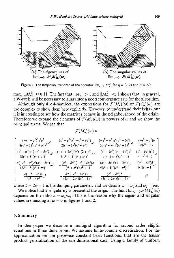
P. W. Hemker / Sparse-grid finite-volume multigrid 109

0 . 0 1 I) 0 ' I

0 . 0 1

0.¢*

l l , l l

o . l ,

* . o l .

(a) The eigenvalues of lime-,0 .f(M~)(~o).

(b) The singular values of lime--.o ~'(M2n)(oa).

Figure 4. The f requency response o f the o p e r a t o r l im ,~ o M . z, for q = (2, 2) and a = 2 /3 .

max~ IIM 211 ~ 0.11. The fact that IIM.II > 1 and IIMffll << l shows that , in general, a W-cycle will be necessary to guarantee a good convergence rate for the algori thm.

A l though only 4 x 4-matrices, the expressions for S ' ( M . ) ( w ) or ~ ( C . ) ( w ) are too complex to show them here explicitly. Howeve r , to unders t and their behav iour it is interest ing to see how the matr ices behave in the n e i g h b o u r h o o d o f the origin. Therefore we expand the elements o f f ( M , ) ( o . , ) in powers o f ~ and we show the principal terms. We see that

Y ( M . ) ( w )

( - d - c~2)2da 2 . j (d + ¢2)~2(-d + 6G 2) ( - d - ¢2)¢4(¢_, _ &2) ( - d - ~2)6 8(e2 + 1)2(e2 + 0.2) 2 2(e2 + i)2(e2 + o.2) 2 co 2a( e2 + o~)2(e 2 + 1) 2 co cr(e 2 + 1)

(E2 + cr2)cr2(_e2 + &p)co 3 (_e2 + 6o.2)22e2(2 + c2) oJ 2 (e2 _ &r2)(a2 _ &2)e2 (~2 _ &~r2)e26w 8(e2 + 8)(e2 + oa) 2 4(e2+l)2(e2+oa) 2 a(e2+oa)2(e2+l) 2~(e2 + 1)

¢(_E2 _ ~2)e2(¢2 _ &2).j (¢2 _ &2)(_e2 + 6o.2)o. ( o2 - 6e2)2( 1 + 2e2) 2 ( °.2 -- 6~2) 6

(8d + 8)(e 2 + oa) 2 (e 2 + a2)2(e 2 + 1) 4(e2 + 1)2(e2 + o.2) 2 w 2e2(~ 2 + 1) w

cr(-¢ 2 - a:2)6 , 6e2(--J + 60"2)Cr (or 2 -- &2)6 62 " 4 ~ ' - + 4 ~ " w- - - ( 2 c 2 + 2 o a ) ( e 2 + l ) W ( 2 e 2 + 2 o a ) ( e 2 + l ) W

where 6 = 2a - 1 is the damping parameter , and we denote w = cv~ and 032 : O'W. We notice that a singulari ty is present at the origin. The limit lim~_~0 . T (M, ) (w)

depends on the rat io a = Wz/~Vl. This is the reason why the eigen- and singular values are missing at w = o in figures 1 and 2.

5. Summary

In this paper we describe a mult igr id a lgor i thm for second order elliptic equat ions in three dimensions. We assume f ini te-volume discretisation, F o r the approx ima t ion we use piecewise cons tan t basis funct ions, that are the tensor p roduc t general isat ion of the one-dimensional case. Using a family o f un i fo rm

110 P. IV. Hemker / Sparse-grid finite-volume multigrid

grids, each member with a different size of support in the different coordinate directions, we obtain a hierarchy of approximations. The corresponding set of function spaces can be interpreted in terms of wavelet terminology as a three-dimensional multiresolution analysis. Following the idea of sparse grids, a selection of degrees of freedom is made, that gives a high accuracy for a relatively small number of degrees of freedom, provided that a certain smoothness requirement is satisfied.

A multigrid algorithm of additive Schwarz type is now constructed for the solution of the discrete system, and its convergence is analysed by Fourier analysis. For this purpose the necessary tools are developed for the Fourier analysis of the box-grid functions.

From the analysis of which the results are summarized in figures 1-4, we conclude that, with simple damped Jacobi iteration as a smoother, the spectral radius of the multigrid iteration matrix is less than 1, uniformly in the cell aspect ratio. In fact, for e the cell aspect ratio, we find max, p(M.) ~ 0.33.

The spectral norm can be larger than one. We find max, IIMnll ~ 5.0. This may indicate that a V-cycle type algorithm will not converge. However, it appears that max, IIM.211 ~ 0.11. This shows that, in general, a W-cycle will be necessary to guarantee a good convergence rate for the algorithm.

References

[1] R.N. Bracewell, The Fourier Transform and its Applications (McGraw-Hill, 1986). [2] I. Daubechies, Ten Lectures on Wavelets, vot. 61 of CBMS-NSF regional conference series in

applied mathematics (SIAM, 1992). [3] M. Griebel, M. Schneider and C. Zenger, A combination technique for the solution of sparse grid

problems, Technical Report TUM-I 9038, SFB 342/19/90A, TU Miinchen (1990). [4] P.W. Hemker, Remarks on sparse-grid finite-volume multigrid, Technical Report NM-R9421,

CWI, Amsterdam (1994). [5] P.W. Hemker and P.M. de Zeeuw, BASIS3: A data structure for 3-dimensional sparse grids,

Technical Report NM-R9321, CWI, Amsterdam (1993). [6] W. Mulder, A high-resolution Euler solver based on multigrid semi-coarsening, and defect

correction, J. Comp. Phys. 100 (1992) 91-104. [7] W.A. Mulder, A new multigrid approach to convection problems, J. Comp. Phys. 17 (1989) 303-

323. [8] N.H. Naik and J. Van Rosendale, The improved robustness of multigrid elliptic solvers based on

multiple semicoarsened grids, Technical Report No. 91-70, ICASE (1991). [9] C. Zenger, Sparse grids, in: Parallel Algorithms for PDE, Proc. 6th GAMM Seminar, ed. W.

Hackbusch, Kiel 1990 (Vieweg, Braunschweig, 1991) pp. 241-251.

Documents

UvA-DARE (Digital Academic Repository) Sparse-Grid … · Sparse-Grid Finite-Volume Multigrid for 3D-Problems ... Sparse-grid finite-volume multigrid for 3D ... algorithm for the