Journal of the Mechanics and Physics of Solids 107 (2017) 343–364

Contents lists available at ScienceDirect

Journal of the Mechanics and Physics of Solids

journal homepage: www.elsevier.com/locate/jmps

A general result for the magnetoelastic response of isotropic

suspensions of iron and ferrofluid particles in rubber, with

applications to spherical and cylindrical specimens

Victor Lefèvre

a , Kostas Danas b , Oscar Lopez-Pamies a , ∗

a Department of Civil and Environmental Engineering, University of Illinois at Urbana-Champaign, United States b LMS, C.N.R.S., École Polytechnique, Université Paris-Saclay, 91128 Palaiseau, France

a r t i c l e i n f o

Article history:

Received 10 April 2017

Revised 10 May 2017

Accepted 25 June 2017

Available online 13 July 2017

Keywords:

Magnetorheological elastomers

Ferrofluid inclusions

Magnetostriction

Finite magnetoelastostatics

a b s t r a c t

This paper puts forth an approximate solution for the effective free-energy function de-

scribing the homogenized (or macroscopic) magnetoelastic response of magnetorheological

elastomers comprised of non-Gaussian rubbers filled with isotropic suspensions of either

iron or ferrofluid particles. The solution is general in that it applies to N = 2 and 3 space

dimensions and any arbitrary (non-percolative) isotropic suspension of filler particles. By

construction, it is exact in the limit of small deformations and moderate magnetic fields.

For finite deformations and finite magnetic fields, its accuracy is demonstrated by means

of direct comparisons with full-field simulations for two prominent cases: ( i ) isotropic sus-

pensions of circular particles and ( ii ) isotropic suspensions of spherical particles.

With the combined objectives of demonstrating the possible benefits of using fer-

rofluid particles in lieu of the more conventional iron particles as fillers and gaining

insight into recent experimental results, the proposed homogenization-based constitutive

model is deployed to generate numerical solutions for boundary-value problems of both

fundamental and practical significance: those consisting of magnetorheological elastomer

specimens of spherical and cylindrical shape that are immersed in air and subjected to a

remotely applied uniform magnetic field. It is found that magnetorheological elastomers

filled with ferrofluid particles can exhibit magnetostrictive capabilities far superior to

those of magnetorheological elastomers filled with iron particles. The results also reveal

that the deformation and magnetic fields are highly heterogenous within the specimens

and strongly dependent on the shape of these, specially for magnetorheological elas-

tomers filled with iron particles. From an applications perspective, this evidence makes it

plain that attempts at designing magnetrostrictive devices based on magnetorheological

elastomers need to be approached, in general, as structural problems, and not simply as

materials design problems.

© 2017 Elsevier Ltd. All rights reserved.

1. Introduction

Ostensibly due to the renewed experimental impetus started during the 1990s (see, e.g., Ginder et al., 1999; Jolly et al.,

1996; Shiga et al., 1995 ), increasing effort s have been devoted by the mechanics community to construct continuum mod-

∗ Corresponding author.

E-mail addresses: vlefevre@illinois.edu (V. Lefèvre), kdanas@lms.polytechnique.fr (K. Danas), pamies@illinois.edu (O. Lopez-Pamies).

http://dx.doi.org/10.1016/j.jmps.2017.06.017

0022-5096/© 2017 Elsevier Ltd. All rights reserved.

344 V. Lefèvre et al. / Journal of the Mechanics and Physics of Solids 107 (2017) 343–364

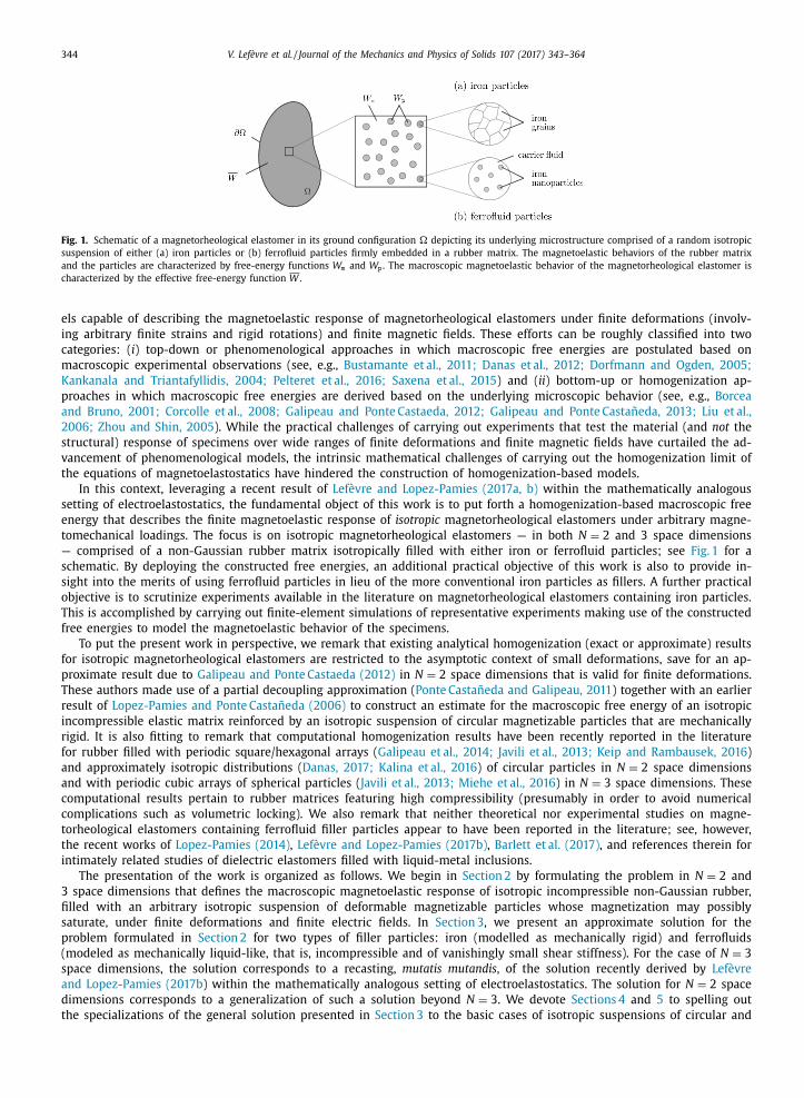
Fig. 1. Schematic of a magnetorheological elastomer in its ground configuration � depicting its underlying microstructure comprised of a random isotropic

suspension of either (a) iron particles or (b) ferrofluid particles firmly embedded in a rubber matrix. The magnetoelastic behaviors of the rubber matrix

and the particles are characterized by free-energy functions W m and W p . The macroscopic magnetoelastic behavior of the magnetorheological elastomer is

characterized by the effective free-energy function W .

els capable of describing the magnetoelastic response of magnetorheological elastomers under finite deformations (involv-

ing arbitrary finite strains and rigid rotations) and finite magnetic fields. These effort s can be roughly classified into two

categories: ( i ) top-down or phenomenological approaches in which macroscopic free energies are postulated based on

macroscopic experimental observations (see, e.g., Bustamante et al., 2011; Danas et al., 2012; Dorfmann and Ogden, 2005;

Kankanala and Triantafyllidis, 2004; Pelteret et al., 2016; Saxena et al., 2015 ) and ( ii ) bottom-up or homogenization ap-

proaches in which macroscopic free energies are derived based on the underlying microscopic behavior (see, e.g., Borcea

and Bruno, 2001; Corcolle et al., 2008; Galipeau and Ponte Castaeda, 2012; Galipeau and Ponte Castañeda, 2013; Liu et al.,

2006; Zhou and Shin, 2005 ). While the practical challenges of carrying out experiments that test the material (and not the

structural) response of specimens over wide ranges of finite deformations and finite magnetic fields have curtailed the ad-

vancement of phenomenological models, the intrinsic mathematical challenges of carrying out the homogenization limit of

the equations of magnetoelastostatics have hindered the construction of homogenization-based models.

In this context, leveraging a recent result of Lefèvre and Lopez-Pamies (2017a, b) within the mathematically analogous

setting of electroelastostatics, the fundamental object of this work is to put forth a homogenization-based macroscopic free

energy that describes the finite magnetoelastic response of isotropic magnetorheological elastomers under arbitrary magne-

tomechanical loadings. The focus is on isotropic magnetorheological elastomers — in both N = 2 and 3 space dimensions

— comprised of a non-Gaussian rubber matrix isotropically filled with either iron or ferrofluid particles; see Fig. 1 for a

schematic. By deploying the constructed free energies, an additional practical objective of this work is also to provide in-

sight into the merits of using ferrofluid particles in lieu of the more conventional iron particles as fillers. A further practical

objective is to scrutinize experiments available in the literature on magnetorheological elastomers containing iron particles.

This is accomplished by carrying out finite-element simulations of representative experiments making use of the constructed

free energies to model the magnetoelastic behavior of the specimens.

To put the present work in perspective, we remark that existing analytical homogenization (exact or approximate) results

for isotropic magnetorheological elastomers are restricted to the asymptotic context of small deformations, save for an ap-

proximate result due to Galipeau and Ponte Castaeda (2012) in N = 2 space dimensions that is valid for finite deformations.

These authors made use of a partial decoupling approximation ( Ponte Castañeda and Galipeau, 2011 ) together with an earlier

result of Lopez-Pamies and Ponte Castañeda (2006) to construct an estimate for the macroscopic free energy of an isotropic

incompressible elastic matrix reinforced by an isotropic suspension of circular magnetizable particles that are mechanically

rigid. It is also fitting to remark that computational homogenization results have been recently reported in the literature

for rubber filled with periodic square/hexagonal arrays ( Galipeau et al., 2014; Javili et al., 2013; Keip and Rambausek, 2016 )

and approximately isotropic distributions ( Danas, 2017; Kalina et al., 2016 ) of circular particles in N = 2 space dimensions

and with periodic cubic arrays of spherical particles ( Javili et al., 2013; Miehe et al., 2016 ) in N = 3 space dimensions. These

computational results pertain to rubber matrices featuring high compressibility (presumably in order to avoid numerical

complications such as volumetric locking). We also remark that neither theoretical nor experimental studies on magne-

torheological elastomers containing ferrofluid filler particles appear to have been reported in the literature; see, however,

the recent works of Lopez-Pamies (2014) , Lefèvre and Lopez-Pamies (2017b) , Barlett et al. (2017) , and references therein for

intimately related studies of dielectric elastomers filled with liquid-metal inclusions.

The presentation of the work is organized as follows. We begin in Section 2 by formulating the problem in N = 2 and

3 space dimensions that defines the macroscopic magnetoelastic response of isotropic incompressible non-Gaussian rubber,

filled with an arbitrary isotropic suspension of deformable magnetizable particles whose magnetization may possibly

saturate, under finite deformations and finite electric fields. In Section 3 , we present an approximate solution for the

problem formulated in Section 2 for two types of filler particles: iron (modelled as mechanically rigid) and ferrofluids

(modeled as mechanically liquid-like, that is, incompressible and of vanishingly small shear stiffness). For the case of N = 3

space dimensions, the solution corresponds to a recasting, mutatis mutandis , of the solution recently derived by Lefèvre

and Lopez-Pamies (2017b ) within the mathematically analogous setting of electroelastostatics. The solution for N = 2 space

dimensions corresponds to a generalization of such a solution beyond N = 3 . We devote Sections 4 and 5 to spelling out

the specializations of the general solution presented in Section 3 to the basic cases of isotropic suspensions of circular and

V. Lefèvre et al. / Journal of the Mechanics and Physics of Solids 107 (2017) 343–364 345

spherical particles and demonstrate their accuracy by confronting them to full-field simulations. In Section 6 , we report

simulations of a boundary-value problem of fundamental importance in its own right that also serves to bring to light the

merits of employing ferrofluid filler particles vs. iron filler particles in magnetorheological elastomers. Finally, in Section 7 ,

we present some comparisons with experiments and record some concluding remarks.

2. The problem

Microscopic description of the material. We are interested in describing the macroscopic magnetoelastic response of a rubber

m atrix filled with a statistically uniform and isotropic suspension of firmly bonded iron or ferrofluid p articles under finite

deformations and finite magnetic fields. This so-called magnetorheological elastomer is taken to occupy a N -dimensional

domain � ⊂ R

N (N = 2 , 3) 1 , with boundary ∂�, in its undeformed, stress-free, and magnetization-free configuration; for

convenience, we choose units of length so that | �| = 1 . The rubber matrix occupies a domain �m , while the particles —

which are taken to be of much smaller sizes than the macroscopic length scale — occupy collectively its complement �p =� \ �m ; see Fig. 1 .

Each material point in the ground configuration � is identified by its initial position vector X , while its position in the

deformed configuration ω is given by x = χ(X ) . We assume that the mapping χ is bijective, continuous, and sufficiently

regular to warrant the mathematical well-posedness of the equations that follow. The corresponding deformation gradient

is denoted by F = Grad χ.

The constitutive behaviors of the matrix and filler particles are taken to be characterized by “total” free-energy functions

( Dorfmann and Ogden, 2004 ) of the deformation gradient F and Lagrangian magnetic field H , in particular, of the (I 1 , I H 5 ) –

based form

W m (F , H ) =

{

�(I 1 ) − μ0

2

I H 5 if J = 1

+ ∞ otherwise (1)

and

W p (F , H ) =

{

G p

2

[ I 1 − N] − S(I H 5 ) if J = 1

+ ∞ otherwise

. (2)

In these expressions, I 1 = F · F , J = det F , I H 5

= F −T H · F −T H , μ0 = 4 π × 10 −7 H / m is the permeability of vacuum, G p stands

for the initial shear modulus of the particles, � denotes any non-negative function of choice (suitably well-behaved) sat-

isfying the linearization conditions �(N) = 0 , � ′ (N) = G/ 2 with G denoting the initial shear modulus of the rubber, 2 and

the function S is also a function of choice satisfying the linearization conditions S(0) = 0 , S ′ (0) = μp / 2 and the convexity

conditions S ′ (I H 5 ) > 0 , S ′ (I H

5 ) + 2 I H

5 S ′′ (I H

5 ) > 0 , where μp stands for the initial permeability of the particles.

Given the free-energy functions (1) and (2) , it follows that the total first Piola-Kirchhoff stress tensor S and Lagrangian

magnetic induction B at any material point X ∈ � are given expediently by the relations

S (X ) =

∂W

∂F (X , F , H ) and B (X ) = −∂W

∂H

(X , F , H ) (3)

with

W (X , F , H ) = [1 − θp (X )] W m (F , H ) + θp (X ) W p (F , H ) , (4)

where θp (X ) is the characteristic function of �p : θp (X ) = 1 if X ∈ �p and zero otherwise. It further follows that the total

Cauchy stress T , Eulerian magnetic induction b , and magnetization m (per unit deformed volume) are in turn given by

T = SF T , b = FB , and m = μ−1 0

b − h with h = F −T H denoting the Eulerian magnetic field. We note that the built-in material

frame indifference of (1) –(2) ensures that T T = T .

Before proceeding with the description of the macroscopic response of the above-defined magnetorheological elas-

tomer, we remark that free-energy functions of the form (1) have been shown to describe reasonably well the response

of a broad variety of rubbers — which are intrinsically non-magnetizable — over wide ranges of deformations (see, e.g.,

Gent, 1996; Lopez-Pamies, 2010; Nunes and Moreira, 2013; Ritto and Nunes, 2015 ). While an analytical result will be pre-

sented in Section 3 that is valid for arbitrary choices of the function � , sample numerical results will be presented in

Sections 4 through 7 for the choice

�(I 1 ) =

N

1 −α1

2 αG 1 [ I

α1

1 − N

α1 ] +

N

1 −α2

2 αG 2 [ I

α2

1 − N

α2 ] . (5)

1 2

1 By considering the cases N = 2 and N = 3 simultaneously, we are able to deal at the same time with suspensions of ( i ) aligned cylindrical fibers and

( ii ) three-dimensional particles. In both cases, we shall refer to the iron or ferrofluid fillers as particles. 2 Throughout this paper, we make use of the standard convention y ′ (x ) = d y (x ) / d x to denote the derivative of functions of a single scalar variable.

346 V. Lefèvre et al. / Journal of the Mechanics and Physics of Solids 107 (2017) 343–364

In this expression, we recall that N stands for the space dimension ( N = 2 , 3 ) and G 1 , G 2 , α1 , α2 are real-valued material

parameters that may be associated with the non-Gaussian statistical distribution of the underlying polymer chains. In addi-

tion to its mathematical simplicity and physical meaning of its parameters, we choose this class of functions because of its

rich functional form and demonstrated descriptive and predictive capabilities ( Lopez-Pamies, 2010 ).

Moreover, free-energy functions of the form (2) are expected to describe reasonably well the finite magnetoelastic re-

sponse of a spectrum of magnetizable filler particles ranging from iron to ferrofluids; while iron has already been widely

utilized as filler particles by the experimental community, the authors are not aware of experiments involving ferrofluid

filler particles (see, however, the device explored by Wang and Gordaninejad (2009) ). We emphasize in particular that free-

energy functions of the form (2) are general enough to model (albeit ignoring dissipative effects) magnetization saturation

phenomena (see, e.g., Arias et al., 2006; Ivanov et al., 2007 ). In this case, granted that the magnetization of the particles is

given by

m p =

[ 2

μ0

S ′ (I H 5 ) − 1

] F −T H , (6)

it must be required, in addition to the linearization and convexity conditions on S mentioned above, that

S ′ (I H 5 ) =

μ0

2

+

μ0 m s

2

√

I H 5

+ o

(1 / √

I H 5

)(7)

in the limit as I H 5

→ ∞ . Here, the positive material constant m s characterizes the magnitude of the saturated magnetization.

While an analytical result will be presented in Section 3 that is valid for any function S of choice, in Sections 4 through

7 sample numerical results will be presented for the Langevin-type function

S(I H 5 ) =

μ0

2

I H 5 +

μ0 m s

βln

⎡ ⎣

sinh

(β√

I H 5

)β√

I H 5

⎤ ⎦ (8)

where β = 3(μp − μ0 ) / (μ0 m s ) , so that

m p =

m s √

I H 5

[

coth

(β√

I H 5

)− 1

β√

I H 5

]

F −T H . (9)

The macroscopic response. In light of the assumed separation of length scales and statistical uniformity of the microstructure,

the microscopically heterogeneous magnetorheological elastomer described above is expected to behave macroscopically as

a homogeneous material. Its macroscopic or overall magnetoelastic response can be defined by the relation between the

volume averages of the first Piola-Kirchhoff stress S and Lagrangian magnetic induction B and the volume averages of the

deformation gradient F and Lagrangian magnetic field H over � when subjected to the affine boundary conditions x = F X

and ψ = −H · X on ∂�, where the second-order tensor F and vector H are prescribed quantities 3 . Thanks to the identities∫ � F (X ) d X = F and

∫ � H (X ) d X = H that follow from the divergence theorem, the derivation of the macroscopic response

reduces then to computing the average Piola-Kirchhoff stress S . =

∫ � S (X ) d X and average Lagrangian magnetic induction

B

. =

∫ � B (X ) d X in terms of F and H . These macroscopic constitutive relations can be conveniently written in the variational

form ( Lopez-Pamies, 2014; Ponte Castañeda and Galipeau, 2011 )

S =

∂ W

∂ F ( F , H ) and B = −∂ W

∂ H

( F , H ) , (10)

where

W ( F , H ) = min

F ∈K max H ∈H

∫ �

W (X , F , H ) d X (11)

denotes the effective free-energy function of the magnetorheological elastomer; in the above expression, K and H stand for

sufficiently large functional spaces of deformation gradients F and curl-free magnetic fields H that are consistent with the

applied affine boundary conditions.

In the present context of magnetoelastostatics, we remark that two of the four relevant governing equations, namely,

balance of linear momentum and Gauss’s law for magnetism,

Div S (X ) = 0 and Div B (X ) = 0 , (12)

correspond to the Euler-Lagrange equations associated with the variational problem (11) . On the other hand, balance of

angular momentum is guaranteed from the material frame indifference of the free-energy functions (1) –(2) , while the choice

of admissible curl-free magnetic fields H in the variational problem (11) ensures that Ampère’s law is satisfied.

3 Here, we have made use of Ampère’s law and represented H as the gradient of a scalar potential, namely, H = −Grad ψ .

V. Lefèvre et al. / Journal of the Mechanics and Physics of Solids 107 (2017) 343–364 347

In analogy with the above relations between the local Lagrangian and Eulerian quantities, it is not difficult to show that

T = S F T , b = F B , and m = μ−1

0 b − h , where T

. = | ω | −1 ∫ ω T (x ) d x , b

. = | ω | −1 ∫ ω b (x ) d x , m

. = | ω | −1 ∫ ω m (x ) d x are the vol-

ume averages of the Cauchy stress T , Eulerian magnetic induction b , and magnetization m over the deformed configuration

ω, while h = F −T

H corresponds to the volume average of the Eulerian magnetic field h over ω.

Isotropic magnetorheological elastomers. Granted the assumed isotropy of the microstructure and the constitutive isotropy

and incompressibility of the rubber and particles, the macroscopic magnetoelastic response of the magnetorheological elas-

tomer is itself isotropic and incompressible. As a result, its effective free energy (11) only depends on the macroscopic

deformation gradient F and macroscopic Lagrangian magnetic field H through 2 N − 1 independent invariants and becomes

unbounded for non-isochoric deformations when J . = det F � = 1 . With a slight abuse of notation, we shall write for N = 2

W ( F , H ) =

{

W ( I 1 , I H

4 , I H

5 ) if J = 1

+ ∞ otherwise , (13)

and for N = 3

W ( F , H ) =

{

W ( I 1 , I 2 , I H

4 , I H

5 , I H

6 ) if J = 1

+ ∞ otherwise , (14)

in terms of the standard invariants

I 1 = F · F , I 2 = F −T · F

−T , I

H

4 = H · H , I H

5 = F −T

H · F −T

H , I H

6 = F −1

F −T

H · F −1

F −T

H . (15)

Note that for N = 2 we have the connections I 2 = I 1 and I H

6 = I 1 I H

5 − I H

4 .

3. An approximate closed-form solution

We put forth in this section a variational solution for the effective free-energy function W defined by the problem (11) .

To this end, exploiting the well-known mathematical analogy between electroelastostatics and magnetoelastostatics (see,

e.g., Stratton, 1941 ), we invoke a solution recently derived by Lefèvre and Lopez-Pamies (2017b ) for the analogous problem

of the nonlinear electroelastic deformation of dielectric elastomer composites in N = 3 space dimensions and recast it mu-

tatis mutandis — as well as extend it to N = 2 — for the nonlinear magnetoelastic deformation of the magnetorheological

elastomers of interest in this work. While the general solution of Lefèvre and Lopez-Pamies (2017b ) applies to deformable

particles with arbitrary initial shear modulus G p ≥ 0 , we restrict the exposition here to the limiting cases of rigid ( G p = + ∞ )

and liquid ( G p = 0 ) particles, which provide reasonable approximations 4 for the iron and ferrofluids fillers of interest in this

work.

The solution. Thus, the effective free-energy function (11) for a rubber with free-energy function (1) , filled with any type of

non-percolative isotropic suspension of rigid ( G p = + ∞ ) or liquid ( G p = 0 ) particles with free-energy function (2) at volume

fraction c , is given by

W ( F , H ) =

{

(1 − c)�( I 1 ) − c S ( I 5 ) +

c νp 2

I 5 +

n −˜ ν

2

I H

4 − ˜ n

2

I H

5 if J = 1

+ ∞ otherwise

(16)

with

I 1 =

s [

I 1 − N

]+ N and I 5 = −1

c

[∂ n

∂νp − ∂ ν

∂νp

]I

H

4 +

1

c

∂ n

∂νp I

H

5 . (17)

Here,

˜ s =

2

(N

2 + N − 2)(1 − c) G

∫ �

g(X ) K klmn �mkl,n d X ,

˜ ν =

1

N

∫ �

μ(X ) γm,m

d X ,

˜ n =

2

N

2 + N − 2

∫ �

μ(X ) K i jkl �ri j,s K rsu v γu,k γv ,l d X (18)

4 The shear modulus of iron is in the order of hundreds of GPas, whereas the shear modulus of a conventional rubber is, at most, in the order of

MPas. On the other hand, ferrofluids are colloidal suspensions of ferromagnetic nanoparticles in a carrier fluid that exhibit near incompressibility and

close-to-zero resistance to shear.

348 V. Lefèvre et al. / Journal of the Mechanics and Physics of Solids 107 (2017) 343–364

with g(X ) =

[1 − θp (X )

]G + θp (X ) G p and μ(X ) =

[1 − θp (X )

]μ0 + θp (X ) νp , where the coefficient 5 νp ≥ μ0 is defined implic-

itly as solution of the nonlinear algebraic equation

2 S ′ ( I 5 ) − νp = 0 , (19)

K i jkl = 1 / 2(δik δ jl + δil δ jk ) − 1 /Nδi j δkl , δij denoting the Kronecker delta, and the tensor fields �(X ) and γ(X ) are defined as

the solutions of the uncoupled linear boundary value problems ⎧ ⎪ ⎨ ⎪ ⎩

[g(X ) K i jmn �mkl,n + δi j q kl

], j

= 0 , X ∈ �

�mkl,m

= 0 , X ∈ �

�ikl = δik X l , X ∈ ∂�

(20)

and { [μ(X ) γi, j

],i

= 0 , X ∈ �

γi = X i , X ∈ ∂�. (21)

In the above expressions, the notation , i represents partial differentiation with respect to the material point coordinate

X i , q (X ) is a tensorial field associated with the incompressibility constraint �mkl,m

= 0 in �, and we recall again that N

stands for the space dimension (N = 2 , 3) , while I 1 , I H

4 , I H

5 stand for the macroscopic invariants defined by expressions

(15) 1, 3, 4 . We refer the interested reader to Section 3 in Lefèvre and Lopez-Pamies (2017b ) for the derivation (for N = 3 )

of the variational solution (16) as well as for a detailed description of its features. Here, it suffices to record the following

remarks:

i. The macroscopic constitutive magnetomechanical relation (10) implied by the free-energy function (16) is given by

S = 2(1 − c) s � ′ (I 1 ) F +

n F −T

H � F −1

F −T

H − p F −T

, (22)

where p stands for the arbitrary hydrostatic pressure associated with the macroscopic incompressibility constraint J = 1 ,

and

B = ( ν −˜ n ) H +

n F −1

F −T

H . (23)

In turn, the macroscopic Cauchy stress, macroscopic Eulerian magnetic induction, and macroscopic magnetization are given

by

T = 2(1 − c) s � ′ (I 1 ) F F T +

n F −T

H � F −T

H − p I ,

b = ( ν −˜ n ) F H +

n F −T

H ,

m =

˜ ν −˜ n

μ0

F H +

n − μ0

μ0

F −T

H , (24)

respectively.

ii. Evaluation of the formula (16) for the effective free energy W and of the formulas (22) and (23) for the macroscopic con-

stitutive relations requires knowledge of the coefficients s , ν, n , νp . All four of them depend on the constitutive behaviors of

the rubber and particles through the material functions/parameters � , μ0 , G p , S and on the microstructure through the so-

lutions �(X ) and γ(X ) of the PDEs (20) –(21) . In addition, the coefficients ν, n , νp depend as well on the magnetomechanical

loading through the invariants I H

4 and I H

5 .

For a given choice of material functions/parameters � , μ0 , G p , S and a given isotropic microstructure, the coefficients s ,˜ ν, ˜ n , νp can be obtained as follows. First, the PDE (20) is solved for �(X ) . In general, this PDE as well as the PDE (21) for

the field γ(X ) do not admit analytical solutions, but can be readily solved numerically using finite elements; see Appendix

B in Lefèvre and Lopez-Pamies (2015) and Appendix A in Spinelli et al. (2015) for details in N = 2 and 3 space dimensions.

Knowledge of �(X ) then allows for the evaluation by means of a quadrature rule of the integral (18) 1 that defines the

effective coefficient ˜ s . As a second step, the PDE (21) is solved for γ(X ) multiple times for a sufficiently wide range of

values of νp ≥ μ0 so as to allow for the numerical computation of the derivatives ∂ ν/∂νp and ∂ n /∂νp entering in (17) 2 , the

numerical solution of the nonlinear algebraic equation (19) defining νp , and the evaluation by means of a quadrature rule

of the integrals (18) 2,3 defining the effective coefficients ν and

n .

In practice, from the above-described numerical construction, it is possible to obtain explicit interpolating formulas

for the coefficients ˜ ν and

˜ n in terms of the coefficient νp . Having access to these formulas reduces the computation of

5 As elaborated in remark ii below, the quantities s , ν, n , νp are not constants but functions of the constitutive behaviors of the rubber matrix and filler

particles, the microstructure, and the last three of them, ν, n , and νp , are also functions of the magnetomechanical loading. We omit these dependencies

for notational simplicity and refer to s , ν, n , νp as “coefficients”.

V. Lefèvre et al. / Journal of the Mechanics and Physics of Solids 107 (2017) 343–36 4 34 9

the effective ener gy (16) and corresponding constitutive relations (22) and (23) simply to solving the nonlinear algebraic

equation (19) for νp . We report such explicit formulas for the basic cases of isotropic suspensions of circular and spherical

particles in Sections 4 and 5 .

iii. By construction, the variational solution (16) is asymptotically exact in the limit of small deformations and moder-

ate magnetic fields, namely, when ε i j . = F i j − δi j = O (ζ ) and H i = O (ζ 1 / 2 ) for a vanishingly small parameter ζ ( Lefèvre

and Lopez-Pamies, 2017a; Tian et al., 2012 ). In this limit, the nonlinear algebraic equation (19) admits the explicit solution

νp = 2 S ′ (0) = μp to leading order, and the effective free energy (16) reduces asymptotically to

W ( F , H ) =

⎧ ⎨ ⎩

(1 − c) G

s ε · ε − ˜ ν

2

H · H +

n H · ε H if tr ε = 0

+ ∞ otherwise

(25)

where, again, the effective coefficients s , ν, n are given by relations (18) with νp = μp .

While, in general, the variational solution (16) is not exact for finite deformations and finite magnetic fields, direct com-

parisons with full-field simulations for the case of N = 3 have shown that it remains accurate for arbitrary magnetomechan-

ical loadings ( Lefèvre and Lopez-Pamies, 2017b ). The accuracy of the variational solution (11) for finite deformations and

finite magnetic fields for the case of N = 2 space dimensions is demonstrated below in Section 4 by analogous comparisons

with full-field simulations.

iv. For the fundamental limiting case when the underlying filler particles are made of a linear magnetic material, so that

S(I H 5 ) =

μp

2

I H 5 , (26)

the equation (19) admits the explicit solution νp = μp and the effective free-energy function (16) reduces rather simply to

W ( F , H ) =

⎧ ⎨ ⎩

(1 − c)�( I 1 ) +

n −˜ ν

2

I H

4 − ˜ n

2

I H

5 if J = 1

+ ∞ otherwise

, (27)

where, again, I 1 is given by expression (17) 1 and the effective constants ν and ˜ n are given by relations (18) 2,3 with νp = μp .

v. Depending on the specific problem at hand, it might be more convenient to employ the macroscopic Lagrangian magnetic

induction B as the independent macroscopic magnetic variable, instead of the magnetic field H . Given that the concavity of

the free-energy functions (1) and (2) in H implies that the effective free-energy function (16) is concave in H within a

possibly unbounded neighborhood of F = I , this can be readily accomplished with help of the partial Legendre transform

W

∗( F , B ) = sup

H

{B · H + W ( F , H )

}, (28)

from which the macroscopic Piola-Kirchhoff stress and the macroscopic Lagrangian magnetic field can be written in terms

of B as follows:

S =

∂ W

∗

∂ F ( F , B ) and H =

∂ W

∗

∂ B

( F , B ) . (29)

Physically, the free energy (28) corresponds to the effective Helmholtz free energy of the magnetorheological elastomer.

As an illustrative example, the partial Legendre transform (28) of the effective free energy (27) for magnetorheological

elastomers with linear magnetic particles renders the effective Helmholtz free energy

W

∗( F , B ) =

⎧ ⎪ ⎨ ⎪ ⎩

(1 − c)�( I 1 ) +

1

2

n

[ ˜ η I B

4 + I B

5

1 +

η 2 +

η I 1

]

if J = 1

+ ∞ otherwise

(30)

for N = 2 , and

W

∗( F , B ) =

⎧ ⎪ ⎨ ⎪ ⎩

(1 − c)�( I 1 ) +

1

2

n

[

I B

5 +

η 2 I B

4 +

η[ I 1 I B

5 − I B

6 ]

1 +

η 3 +

η 2 I 2 +

ηI 1

]

if J = 1

+ ∞ otherwise

(31)

for N = 3 . In these last expressions, the coefficient ˜ η = ( ν −˜ n ) / n has been introduced to ease notation, I B

4 , I B

5 , I B

6 stand for

the standard invariants

I B

4 = B · B , I B

5 = F B · F B , I B

6 = F T

F B · F T

F B , (32)

and it is recalled that I 1 is given by expression (17) 1 , while the effective constants ν and ˜ n are given by (18) 2,3 with νp = μp .

350 V. Lefèvre et al. / Journal of the Mechanics and Physics of Solids 107 (2017) 343–364

vi. We remark that for the case of N = 2 space dimensions, the (finite branch of the) effective free energy (16) is of the

separable form W = W elas ( I 1 ) + W mag ( I H

4 , I H

5 ) . By contrast, when written in terms of F and B as the independent variables,

it is not difficult to deduce that the (finite branch of the) corresponding Helmholtz free energy (28) is of the general non-

separable form W

∗ = W

∗( I 1 , I

B

4 , I B

5 ) ; see, for instance, the Helmholtz free energy (30) .

For the case of N = 3 , the (finite branch of the) effective free energy (16) is also of the separable form W = W elas ( I 1 ) +W mag ( I

H

4 , I H

5 ) , but, interestingly, it only depends on three of the five isotropic invariants (15) . By contrast, the (finite branch

of the) corresponding Helmholtz free energy (28) is of the general non-separable form W

∗ = W

∗( I 1 , I 2 , I

B

4 , I B

5 , I B

6 ) ; see, for

instance, the Helmholtz free energy (31) .

The above-outlined homogenization-based functional dependencies on the standard invariants I 1 , I 2 , I H

4 , I H

5 , I H

6 , I B

4 , I B

5 ,

I B

6 differ from the phenomenological ones that have been suggested/utilized in the literature based on the limited available

experimental data; see, e.g., the works of Dorfmann and Ogden (2005) , Bustamante et al. (2011) , and Pelteret et al. (2016) .

4. The basic case of an isotropic suspension of circular particles

In this section, we present the specialization of the effective free energy (16) to the basic case in N = 2 space dimensions

of magnetorheological elastomers wherein the isotropically distributed filler particles are monodisperse in size and circular

in shape. We begin by presenting in Section 4.1 the result for circular iron particles and confront it with full-field simula-

tions to demonstrate its accuracy for finite deformations and finite magnetic fields. The same is done in Section 4.2 for the

specialization to circular ferrofluid particles.

Before proceeding with the presentation of the results, we recall that explicit interpolating formulas for the coefficients˜ ν and ˜ n in terms of the coefficient νp can be obtained via the numerical construction outlined in remark ii of Section 3 .

Repeating these calculations for various volume fractions of particles c allows, moreover, to obtain explicit interpolating

formulas for ν and

n , as well as for the coefficient s , in terms of c . We shall present below such formulas for iron as well as

for ferrofluid circular particles. Again, having access to these formulas reduces the computation of the effective energy (16) ,

and the corresponding constitutive relations (22) and (23) , simply to solving the nonlinear algebraic equation (19) for νp .

4.1. The solution for circular iron particles

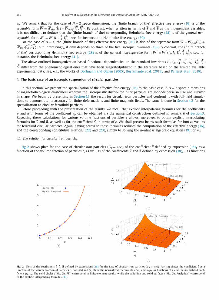
Fig. 2 shows plots for the case of circular iron particles ( G p = + ∞ ) of the coefficient ˜ s defined by expression (18) 1 as a

function of the volume fraction of particles c , as well as of the coefficients ν and

n defined by expression (18) 2,3 as functions

Fig. 2. Plots of the coefficients s , ν, n defined by expressions (18) for the case of circular iron particles ( G p = + ∞ ). Part (a) shows the coefficient s as a

function of the volume fraction of particles c . Parts (b) and (c) show the normalized coefficients ν/μ0 and n /μ0 as functions of c and the normalized coef-

ficient μ0 /νp . The solid circles (“Rig. Cir. FE”) correspond to finite-element results, while the solid line and solid surfaces (“Rig. Cir. Analytical”) correspond

to the explicit interpolating formulas (33) .

V. Lefèvre et al. / Journal of the Mechanics and Physics of Solids 107 (2017) 343–364 351

of c and the coefficient νp . The solid circles (labeled as “Rig. Cir. FE” in the plots) correspond to results 6 based on finite-

element solutions of the PDEs (20) and (21) for the fields �(X ) and γ(X ) , while the solid line and solid surfaces (labeled as

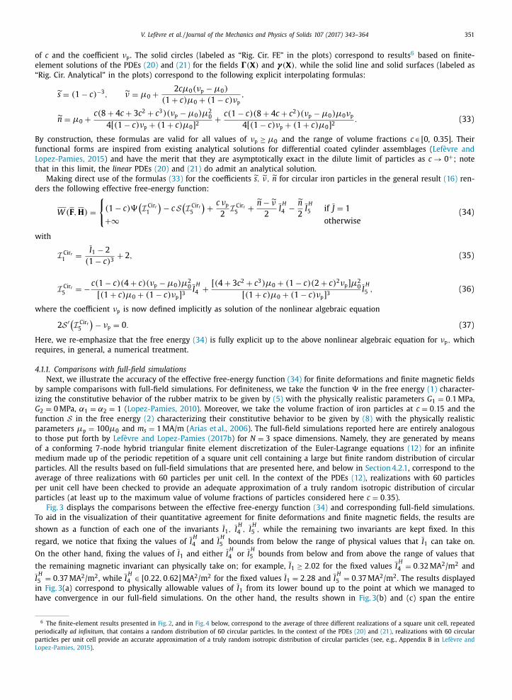
“Rig. Cir. Analytical” in the plots) correspond to the following explicit interpolating formulas:

˜ s = (1 − c) −3 , ˜ ν = μ0 +

2 cμ0 (νp − μ0 )

(1 + c) μ0 + (1 − c) νp ,

˜ n = μ0 +

c(8 + 4 c + 3 c 2 + c 3 )(νp − μ0 ) μ2 0

4[(1 − c) νp + (1 + c) μ0 ] 2 +

c(1 − c)(8 + 4 c + c 2 )(νp − μ0 ) μ0 νp 4[(1 − c) νp + (1 + c) μ0 ] 2

. (33)

By construction, these formulas are valid for all values of νp ≥ μ0 and the range of volume fractions c ∈ [0, 0.35]. Their

functional forms are inspired from existing analytical solutions for differential coated cylinder assemblages ( Lefèvre and

Lopez-Pamies, 2015 ) and have the merit that they are asymptotically exact in the dilute limit of particles as c → 0 + ; note

that in this limit, the linear PDEs (20) and (21) do admit an analytical solution.

Making direct use of the formulas (33) for the coefficients s , ν, n for circular iron particles in the general result (16) ren-

ders the following effective free-energy function:

W ( F , H ) =

{

(1 − c)�(I Cir r

1

)− c S

(I Cir r

5

)+

c νp 2

I Cir r 5

+

n −˜ ν

2

I H

4 − ˜ n

2

I H

5 if J = 1

+ ∞ otherwise (34)

with

I Cir r 1

=

I 1 − 2

(1 − c) 3 + 2 , (35)

I Cir r 5

= − c(1 − c)(4 + c)(νp − μ0 ) μ2 0

[(1 + c) μ0 + (1 − c) νp ] 3 I

H

4 +

[(4 + 3 c 2 + c 3 ) μ0 + (1 − c)(2 + c) 2 νp ] μ2 0

[(1 + c) μ0 + (1 − c) νp ] 3 I

H

5 , (36)

where the coefficient νp is now defined implicitly as solution of the nonlinear algebraic equation

2 S ′ (I Cir r

5

)− νp = 0 . (37)

Here, we re-emphasize that the free energy (34) is fully explicit up to the above nonlinear algebraic equation for νp , which

requires, in general, a numerical treatment.

4.1.1. Comparisons with full-field simulations

Next, we illustrate the accuracy of the effective free-energy function (34) for finite deformations and finite magnetic fields

by sample comparisons with full-field simulations. For definiteness, we take the function � in the free energy (1) character-

izing the constitutive behavior of the rubber matrix to be given by (5) with the physically realistic parameters G 1 = 0 . 1 MPa,

G 2 = 0 MPa, α1 = α2 = 1 ( Lopez-Pamies, 2010 ). Moreover, we take the volume fraction of iron particles at c = 0 . 15 and the

function S in the free energy (2) characterizing their constitutive behavior to be given by (8) with the physically realistic

parameters μp = 100 μ0 and m s = 1 MA/m ( Arias et al., 2006 ). The full-field simulations reported here are entirely analogous

to those put forth by Lefèvre and Lopez-Pamies (2017b ) for N = 3 space dimensions. Namely, they are generated by means

of a conforming 7-node hybrid triangular finite element discretization of the Euler-Lagrange equations (12) for an infinite

medium made up of the periodic repetition of a square unit cell containing a large but finite random distribution of circular

particles. All the results based on full-field simulations that are presented here, and below in Section 4.2.1 , correspond to the

average of three realizations with 60 particles per unit cell. In the context of the PDEs (12) , realizations with 60 particles

per unit cell have been checked to provide an adequate approximation of a truly random isotropic distribution of circular

particles (at least up to the maximum value of volume fractions of particles considered here c = 0 . 35 ).

Fig. 3 displays the comparisons between the effective free-energy function (34) and corresponding full-field simulations.

To aid in the visualization of their quantitative agreement for finite deformations and finite magnetic fields, the results are

shown as a function of each one of the invariants I 1 , I H

4 , I H

5 , while the remaining two invariants are kept fixed. In this

regard, we notice that fixing the values of I H

4 and I H

5 bounds from below the range of physical values that I 1 can take on.

On the other hand, fixing the values of I 1 and either I H

4 or I H

5 bounds from below and from above the range of values that

the remaining magnetic invariant can physically take on; for example, I 1 ≥ 2 . 02 for the fixed values I H

4 = 0 . 32 MA

2 /m

2 and

I H

5 = 0 . 37 MA

2 /m

2 , while I H

4 ∈ [0 . 22 , 0 . 62] MA

2 /m

2 for the fixed values I 1 = 2 . 28 and I H

5 = 0 . 37 MA

2 /m

2 . The results displayed

in Fig. 3 (a) correspond to physically allowable values of I 1 from its lower bound up to the point at which we managed to

have convergence in our full-field simulations. On the other hand, the results shown in Fig. 3 (b) and (c) span the entire

6 The finite-element results presented in Fig. 2 , and in Fig. 4 below, correspond to the average of three different realizations of a square unit cell, repeated

periodically ad infinitum , that contains a random distribution of 60 circular particles. In the context of the PDEs (20) and (21) , realizations with 60 circular

particles per unit cell provide an accurate approximation of a truly random isotropic distribution of circular particles (see, e.g., Appendix B in Lefèvre and

Lopez-Pamies, 2015 ).

352 V. Lefèvre et al. / Journal of the Mechanics and Physics of Solids 107 (2017) 343–364

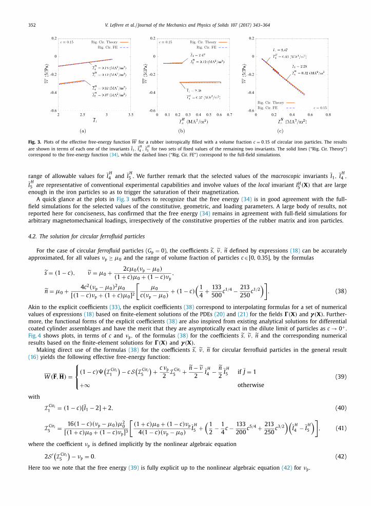
Fig. 3. Plots of the effective free-energy function W for a rubber isotropically filled with a volume fraction c = 0 . 15 of circular iron particles. The results

are shown in terms of each one of the invariants I 1 , I H

4 , I H

5 for two sets of fixed values of the remaining two invariants. The solid lines (“Rig. Cir. Theory”)

correspond to the free-energy function (34) , while the dashed lines (“Rig. Cir. FE”) correspond to the full-field simulations.

range of allowable values for I H

4 and I H

5 . We further remark that the selected values of the macroscopic invariants I 1 , I H

4 ,

I H

5 are representative of conventional experimental capabilities and involve values of the local invariant I H 5 (X ) that are large

enough in the iron particles so as to trigger the saturation of their magnetization.

A quick glance at the plots in Fig. 3 suffices to recognize that the free energy (34) is in good agreement with the full-

field simulations for the selected values of the constitutive, geometric, and loading parameters. A large body of results, not

reported here for conciseness, has confirmed that the free energy (34) remains in agreement with full-field simulations for

arbitrary magnetomechanical loadings, irrespectively of the constitutive properties of the rubber matrix and iron particles.

4.2. The solution for circular ferrofluid particles

For the case of circular ferrofluid particles ( G p = 0 ), the coefficients s , ˜ ν, ˜ n defined by expressions (18) can be accurately

approximated, for all values νp ≥ μ0 and the range of volume fraction of particles c ∈ [0, 0.35], by the formulas

˜ s = (1 − c) , ˜ ν = μ0 +

2 cμ0 (νp − μ0 )

(1 + c) μ0 + (1 − c) νp ,

˜ n = μ0 +

4 c 2 (νp − μ0 ) 2 μ0

[(1 − c) νp + (1 + c) μ0 ] 2

[μ0

c(νp − μ0 ) + (1 − c)

(1

4

+

133

500

c 1 / 4 − 213

250

c 1 / 2 )]

. (38)

Akin to the explicit coefficients (33) , the explicit coefficients (38) correspond to interpolating formulas for a set of numerical

values of expressions (18) based on finite-element solutions of the PDEs (20) and (21) for the fields �(X ) and γ(X ) . Further-

more, the functional forms of the explicit coefficients (38) are also inspired from existing analytical solutions for differential

coated cylinder assemblages and have the merit that they are asymptotically exact in the dilute limit of particles as c → 0 + .Fig. 4 shows plots, in terms of c and νp , of the formulas (38) for the coefficients ˜ s , ˜ ν, ˜ n and the corresponding numerical

results based on the finite-element solutions for �(X ) and γ(X ) .

Making direct use of the formulas (38) for the coefficients ˜ s , ˜ ν, ˜ n for circular ferrofluid particles in the general result

(16) yields the following effective free-energy function:

W ( F , H ) =

⎧ ⎨ ⎩

(1 − c)�(I Cir l

1

)− c S

(I Cir l

5

)+

c νp 2

I Cir l 5

+

n −˜ ν

2

I H

4 − ˜ n

2

I H

5 if J = 1

+ ∞ otherwise

(39)

with

I Cir l 1

= (1 − c)[ I 1 − 2] + 2 , (40)

I Cir l 5

=

16(1 − c)(νp − μ0 ) μ2 0

[(1 + c) μ0 + (1 − c) νp ] 3

[(1 + c) μ0 + (1 − c) νp

4(1 − c)(νp − μ0 ) I

H

5 +

(1

2

− 1

4

c − 133

200

c 5 / 4 +

213

250

c 3 / 2 )(

I H

4 − I H

5

)], (41)

where the coefficient νp is defined implicitly by the nonlinear algebraic equation

2 S ′ (I Cir l

5

)− νp = 0 . (42)

Here too we note that the free energy (39) is fully explicit up to the nonlinear algebraic equation (42) for νp .

V. Lefèvre et al. / Journal of the Mechanics and Physics of Solids 107 (2017) 343–364 353

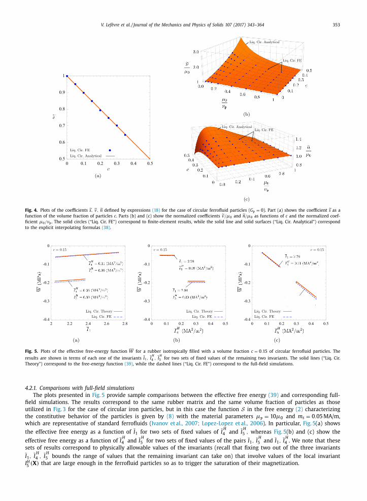
Fig. 4. Plots of the coefficients s , ν, n defined by expressions (18) for the case of circular ferrofluid particles ( G p = 0 ). Part (a) shows the coefficient s as a

function of the volume fraction of particles c . Parts (b) and (c) show the normalized coefficients ν/μ0 and n /μ0 as functions of c and the normalized coef-

ficient μ0 /νp . The solid circles (“Liq. Cir. FE”) correspond to finite-element results, while the solid line and solid surfaces (“Liq. Cir. Analytical”) correspond

to the explicit interpolating formulas (38) .

Fig. 5. Plots of the effective free-energy function W for a rubber isotropically filled with a volume fraction c = 0 . 15 of circular ferrofluid particles. The

results are shown in terms of each one of the invariants I 1 , I H

4 , I H

5 for two sets of fixed values of the remaining two invariants. The solid lines (“Liq. Cir.

Theory”) correspond to the free-energy function (39) , while the dashed lines (“Liq. Cir. FE”) correspond to the full-field simulations.

4.2.1. Comparisons with full-field simulations

The plots presented in Fig. 5 provide sample comparisons between the effective free energy (39) and corresponding full-

field simulations. The results correspond to the same rubber matrix and the same volume fraction of particles as those

utilized in Fig. 3 for the case of circular iron particles, but in this case the function S in the free energy (2) characterizing

the constitutive behavior of the particles is given by (8) with the material parameters μp = 10 μ0 and m s = 0 . 05 MA/m,

which are representative of standard ferrofluids ( Ivanov et al., 2007; Lopez-Lopez et al., 2006 ). In particular, Fig. 5 (a) shows

the effective free energy as a function of I 1 for two sets of fixed values of I H

4 and I H

5 , whereas Fig. 5 (b) and (c) show the

effective free energy as a function of I H

4 and I H

5 for two sets of fixed values of the pairs I 1 , I H

5 and I 1 , I H

4 . We note that these

sets of results correspond to physically allowable values of the invariants (recall that fixing two out of the three invariants

I 1 , I H

4 , I H

5 bounds the range of values that the remaining invariant can take on) that involve values of the local invariant

I H (X ) that are large enough in the ferrofluid particles so as to trigger the saturation of their magnetization.

5

354 V. Lefèvre et al. / Journal of the Mechanics and Physics of Solids 107 (2017) 343–364

It is plain from Fig. 5 that the free energy (39) is in good quantitative and qualitative agreement with the full-field

simulations for the selected values of the constitutive, geometric, and loading parameters. A spectrum of results beyond

those reported here has confirmed that the free energy (39) remains in agreement with full-field simulations for arbitrary

magnetomechanical loadings, irrespectively of the constitutive properties of the rubber matrix and ferrofluid particles.

5. The basic case of an isotropic suspension of spherical particles

In the sequel, we report the specialization of the free energy (16) to the basic case in N = 3 space dimensions of magne-

torheological elastomers wherein the isotropically distributed filler particles are monodisperse in size and spherical in shape.

We present the result for spherical iron particles in Section 5.1 and that for spherical ferrofluid particles in Section 5.2 . We

note that the accuracy of both of these results has already been demonstrated — within the mathematically analogous set-

ting of elastic dielectric composites — for finite deformations and finite magnetic fields via direct comparisons with full-field

simulations in Section 6 of Lefèvre and Lopez-Pamies (2017b ). Accordingly, we do not reproduce such comparisons here.

5.1. The solution for spherical iron particles

For the case of spherical iron particles ( G p = + ∞ ), the coefficients s , ˜ ν, ˜ n defined by expressions (18) can be accurately

approximated, for all values of the coefficient νp ≥ μ0 and the range of volume fraction of particles c ∈ [0, 0.25], by the

formulas

˜ s = (1 − c) −7 / 2 , ˜ ν = μ0 +

3 cμ0 (νp − μ0 )

(2 + c) μ0 + (1 − c) νp ,

˜ n = μ0 +

3 c(10 + 2 c + 3 c 2 )(νp − μ0 ) μ2 0

5[(2 + c) μ0 + (1 − c) νp ] 2 +

3 c(1 − c)(5 + 3 c)(νp − μ0 ) μ0 νp 5[(2 + c) μ0 + (1 − c) νp ] 2

. (43)

Upon direct use of these explicit expressions, the general result (16) specializes to the following effective free-energy func-

tion:

W ( F , H ) =

⎧ ⎨ ⎩

(1 − c)�(I Sph r

1

)− c S

(I Sph r

5

)+

c νp 2

I Sph r 5

+

n −˜ ν

2

I H

4 − ˜ n

2

I H

5 if J = 1

+ ∞ otherwise

(44)

with

I Sph r 1

=

I 1 − 3

(1 − c) 7 / 2 + 3 , (45)

I Sph r 5

= − 54 c(1 − c)(νp − μ0 ) μ2 0

5[(2 + c) μ0 + (1 − c) νp ] 3 I

H

4 +

9[(10 − c + 6 c 2 ) μ0 + (5 + c − 6 c 2 ) νp ] μ2 0

5[(2 + c) μ0 + (1 − c) νp ] 3 I

H

5 , (46)

where the coefficient νp is defined implicitly as solution of the nonlinear algebraic equation

2 S ′ (I Sph r

5

)− νp = 0 . (47)

Similar to its counterpart (34) for circular iron particles, the free energy (44) is fully explicit up the nonlinear algebraic

equation (47) for νp .

5.2. The solution for spherical ferrofluid particles

Finally, for the case of spherical ferrofluid particles ( G p = 0 ), the coefficients ˜ s , ˜ ν, ˜ n defined by expressions (18) can be

accurately approximated by the formulas

˜ s = (1 − c) 2 / 3 , ˜ ν = μ0 +

3 cμ0 (νp − μ0 )

(2 + c) μ0 + (1 − c) νp ,

˜ n = μ0 +

9 c 2 (νp − μ0 ) 2 μ0

[(2 + c) μ0 + (1 − c) νp ] 2

[4

45

− 81 c 11 / 25

500

+

μ0

c(νp − μ0 )

], (48)

which are valid for all values of the coefficient νp ≥ μ0 and the range of volume fraction of particles c ∈ [0, 0.25]. Much like

the explicit coefficients (43) , the explicit coefficients (48) correspond to interpolating formulas based on a set of numer-

ical values of expressions (18) generated from finite-element solutions of the PDEs (20) and (21) for the fields �(X ) and

γ(X ) . The coefficients (48) also draw their functional forms from existing analytical solutions for differential coated sphere

assemblages ( Lefèvre and Lopez-Pamies, 2014 ) and are asymptotically exact in the dilute limit as c → 0 + .

V. Lefèvre et al. / Journal of the Mechanics and Physics of Solids 107 (2017) 343–364 355

Direct use of the formulas (48) for the coefficients s , ν, n for spherical ferrofluid particles in the general result (16) leads

to the following effective free-energy function:

W ( F , H ) =

⎧ ⎨ ⎩

(1 − c)�(I Sph l

1

)− c S

(I Sph l

5

)+

c νp 2

I Sph l 5

+

n −˜ ν

2

I H

4 − ˜ n

2

I H

5 if J = 1

+ ∞ otherwise

(49)

with

I Sph l 1

= (1 − c) 2 / 3 ( I 1 − 3) + 3 , (50)

I Sph l 5

=

3(1500 − 1900 c + 729 c 36 / 25 )(νp − μ0 ) μ2 0

250[(2 + c) μ0 + (1 − c) νp ] 3 I

H

4 − 3[(750 − 1150 c + 729 c 36 / 25 )(νp − μ0 ) − 2250 μ0 ] μ2 0

250[(2 + c) μ0 + (1 − c) νp ] 3 I

H

5 ,

(51)

where the coefficient νp is now defined implicitly by the nonlinear algebraic equation

2 S ′ (I Sph l

5

)− νp = 0 . (52)

Similar to its counterpart (39) for circular ferrofluid particles, the effective free energy (49) is fully explicit up to the numer-

ical treatment required, in general, to compute the coefficient νp from its implicit definition (52) .

6. Iron particles vs. ferrofluid particles

Since the classical work of Brown (1966) , it is well known that a homogeneous magnetoelastic specimen of ellipsoidal

shape does not deform uniformly when exposed to a remotely applied homogeneous magnetic field. 7 In spite of the fun-

damental nature of this Eshelby-type boundary-value problem, its solution does not appear to have been reported in the

literature; see, however, Sections 10.2–10.4 of Chapter IV in Brown (1966) and references therein for a number of partial

solutions in the asymptotic context of small deformations. Leveraging the general result (16) for the effective free energy of

isotropic magnetorheological elastomers, the compound objective of this section is to present such a solution — which, by

necessity, is numerical — and to gain insight into the magnetoelastic behavior of magnetorheological elastomers containing

ferrofluid filler particles vis-à-vis that of magnetorheological elastomers containing iron filler particles.

For definiteness, we consider the boundary-value problem of a specimen of initial spherical shape and unit radius im-

mersed in an infinite medium otherwise filled by air that is subjected to a remotely applied homogeneous magnetic field,

H ∞

say. The specimen is made up of an isotropic magnetorheological elastomer whose magnetoelastic behavior is char-

acterized by either the effective free-energy function (44) corresponding to spherical iron filler particles or the effective

free-energy function (49) corresponding to spherical ferrofluid filler particles. For convenience, among the various possi-

ble modeling strategies, we opt to model the surrounding a ir as a compressible magnetoelastic material of vanishing small

mechanical stiffness with free-energy function

W a (F , H ) =

G a

2

[ I 1 − 3 − 2 ln J] − μ0

2

JI H 5 with G a = 0

+ , (53)

where we recall that I 1 = F · F , J = det F , I H 5

= F −T H · F −T H , and μ0 = 4 π × 10 −7 H/m. Thus, more precisely, we are interested

in solving the boundary-value problem ⎧ ⎪ ⎪ ⎨ ⎪ ⎪ ⎩

Div S (X ) = 0 , X ∈ R

3

Div B (X ) = 0 , X ∈ R

3

χ(X ) = X , || X || → ∞

ψ(X ) = −H ∞

· X , || X || → ∞

, (54)

where

S (X ) = θ (X ) ∂ W

∂F (F , H ) + ( 1 − θ (X ) )

∂W a

∂F (F , H ) (55)

and

B (X ) = −θ (X ) ∂ W

∂H

(F , H ) − ( 1 − θ (X ) ) ∂W a

∂H

(F , H ) (56)

with θ (X ) = 1 if | X | ≤ 1 and zero otherwise, for the deformation field χ(X ) and the magnetic potential ψ( X ). In the above

expressions, again, the effective free-energy function W is given by (44) for the case of magnetorheological elastomers

7 Specifically, the classical result of Brown (1966) applies to finite deformations, finite magnetic fields, and any anisotropic magnetoelastic solid featuring

orthotropic material symmetry; see Section 10.1 of Chapter IV in Brown (1966) .

356 V. Lefèvre et al. / Journal of the Mechanics and Physics of Solids 107 (2017) 343–364

Fig. 6. (a) Schematic of the finite domain utilized to generate numerical solutions for the boundary-value problem (54) . The air domain is defined by an

initial outer radius that is twenty times that of the spherical specimen. (b) Detail of the corresponding axisymmetric discretization with 7-node hybrid

triangular finite elements.

wherein the fillers are spherical iron particles and by (49) for the case of magnetorheological elastomers wherein the fillers

are spherical ferrofluid particles.

For computational expediency, we seek to generate numerical solutions for the boundary-value problem (54) on a spatial

domain of sufficiently large but finite extent, and not on R

3 in its entirety. To this end, we find it convenient to consider a

domain that consists of the specimen surrounded by an air-filled thick spherical shell that is subjected on its external surface

to the affine deformation x = X and the affine magnetic potential ψ = −H ∞

· X ; such a computational domain is schemati-

cally depicted in Fig. 6 (a). A parametric study has revealed that a domain of this kind with initial outer radius twenty times

larger than the initial radius of the specimen is large enough to accurately reproduce the solution of the boundary-value

problem (54) , at least for the choices of material and loading parameters of interest here. The study has also revealed that an

initial shear modulus of the air that is three orders of magnitude smaller than that of the rubber utilized for the specimen

— namely, G a = 10 −3 G — is small enough to be representative of G a = 0 + . Now, given the axial symmetry of the problem

around the direction of the applied magnetic field H ∞

, it proves useful to select the frame of reference so that H ∞

= H ∞

e 3 .

In this context, accurate numerical solutions can be efficiently generated by means of a conforming axisymmetric 7-node

hybrid triangular finite element discretization on meshes comprising about 160,0 0 0 elements such as the one illustrated in

Fig. 6 (b). The representative solutions that we present next were generated based on such a discretization. All of these solu-

tions correspond to specimens with the same rubber matrix, for which the function � is given by (5) with the parameters

G 1 = 0 . 1 MPa, G 2 = 0 MPa, α1 = α2 = 1 , and the same volume fraction of filler particles c = 0 . 20 . For specimens wherein the

fillers are spherical iron particles, the solutions correspond to the choice (8) for the function S in (44) with the parameters

μp = 100 μ0 and m s = 1 . 0 MA/m. On the other hand, for specimens wherein the fillers are spherical ferrofluid particles, the

solutions correspond to the choice (8) for the function S in (49) with the parameters μp = 10 μ0 and m s = 0 . 1 , 0 . 3 , 0 . 5 MA/m.

Figs. 7 (a)–(c) present contour plots in the e 1 –e 3 plane of the component F 33 ( X ) of the local deformation gradient over

the specimen of the magnetorheological elastomer with iron filler particles at the three values of the applied magnetic

field H ∞

= 0 . 11 , 0 . 26 , and 1.00 MA/m. Figs. 7 (d)–(f) present the analogous contour plots for the specimen containing fer-

rofluid filler particles with magnetization saturation m s = 0 . 3 MA/m. As already established by Brown (1966) , an immediate

observation from these contour plots is that the deformation gradient in the specimens is not uniform, increasingly so

for increasing values of the applied magnetic field. We notice in particular that the core of the magnetorheological elas-

tomer with iron particles undergoes extension ( F 33 ( X ) > 1), while its poles are under compression ( F 33 ( X ) < 1). This exten-

sion/compression heterogeneity increases substantially and monotonically with the applied magnetic field. At the largest

value H ∞

= 1 . 00 MA/m of the applied magnetic field, when the specimen happens to have already reached a saturated state

of magnetization, F 33 (X ) = 1 . 024 at the center of the specimen while F 33 (X ) = 0 . 981 at the poles. By contrast, the mag-

netorheological elastomer with ferrofluid particles, which exhibits a lesser degree of heterogeneity throughout the entire

magnetic loading process, is under extension ( F 33 ( X ) > 1) at every material point. The largest and smallest extensions oc-

cur at the center and at the poles of the specimen, respectively. For instance, at the largest value H ∞

= 1 . 00 MA/m of the

applied magnetic field, the specimen attains the value F 33 (X ) = 1 . 039 at its center and F 33 (X ) = 1 . 028 at its poles. By com-

paring these extremal values to those of the magnetorheological elastomer with iron particles, it is plain that the use of

ferrofluid filler particles — in lieu of the more conventional iron filler particles — in magnetorheological elastomers can lead

to significantly superior magnetostrictive properties.

To gain further quantitative insight into the enhancement of magnetostrictive properties afforded by ferrofluid particles,

we plot in Fig. 8 (a) the average deformation gradient 〈 F 33 (X ) 〉 . = ( ∫

3 θ (X )d X ) −1 ∫

3 θ (X ) F 33 (X )d X , or average magnetostric-

R R

V. Lefèvre et al. / Journal of the Mechanics and Physics of Solids 107 (2017) 343–364 357

Fig. 7. Contour plots of the component F 33 ( X ) of the deformation gradient over spherical specimens of magnetorheological elastomers containing c = 0 . 20

volume fraction of: (a)–(c) spherical iron filler particles and (d)–(f) spherical ferrofluid filler particles (with magnetization saturation m s = 0 . 3 MA/m). The

contours correspond to the remotely applied magnetic field H ∞ = H ∞ e 3 with H ∞ = 0 . 11 , 0 . 26 , 1.00 MA/m and, as implied by the argument X in F 33 ( X ), are

shown over the undeformed configuration of the specimens. The color scale bars in each of the contour plots indicate the corresponding variation of F 33 ( X )

from its minimum to its maximum value.

Fig. 8. (a) Average magnetostriction 〈 F 33 ( X ) 〉 as a function of the applied magnetic field H ∞ for the same two specimens discussed in Fig. 7 . (b) Average

magnetostriction 〈 F 33 ( X ) 〉 as a function of the applied magnetic field H ∞ for spherical specimens of magnetorheological elastomers containing c = 0 . 20

volume fraction of spherical ferrofluid filler particles with magnetization saturation m s = 0 . 1 , 0 . 3 , and 0.5 MA/m.

tion, as a function of the applied magnetic field H ∞

for the two specimens shown in Fig. 7 . As expected from the preceding

observations about the local deformation, the plot shows that the specimen with ferrofluid filler particles exhibits an average

magnetostriction of extension ( 〈 F 33 ( X ) 〉 > 1) that is significantly larger than that of the specimen with iron filler particles;

interestingly, the average magnetostriction of the latter is also of extension. Furthermore, we remark that the average mag-

netostriction saturates in both specimens as the magnetic field increases, but that in the specimen with ferrofluid filler

particles the saturation is reached at a significantly smaller value of the applied magnetic field. A parametric study varying

the magnetization saturation parameter m s of the ferrofluid has indicated that the saturated value of the average magne-

tostriction, 〈 F 33 ( X ) 〉 sat say, can be increased significantly by increasing the value of m s . This point is illustrated by Fig. 8 (b),

where analogous results to that presented in Fig. 8 (a) are plotted for specimens containing ferrofluid filler particles with

m s = 0 . 1 , 0 . 3 , and 0.5 MA/m. These encouraging sample results are supportive of further investigations of magnetorheologi-

cal elastomers containing ferrofluid filler particles.

358 V. Lefèvre et al. / Journal of the Mechanics and Physics of Solids 107 (2017) 343–364

Fig. 9. Contour plots of the component H 3 ( X ) of the Lagrangian magnetic field from the same simulations as in Fig. 7 over spherical specimens of mag-

netorheological elastomers containing c = 0 . 20 volume fraction of: (a)–(c) spherical iron filler particles and (d)–(f) spherical ferrofluid filler particles (with

magnetization saturation m s = 0 . 3 MA/m). The contours correspond to the remotely applied magnetic field H ∞ = H ∞ e 3 with H ∞ = 0 . 11 , 0 . 26 , 1.00 MA/m

and, as implied by the argument X in H 3 ( X ), are shown over the undeformed configuration of the specimens. The color scale bars in each of the contour

plots indicate the corresponding variation of H 3 ( X ) from its minimum to its maximum value.

We close this section, for completeness, by presenting in Fig. 9 the contour plots of the component H 3 ( X ) of the La-

grangian magnetic field over the same two spherical specimens discussed in Fig. 7 . Similar to the deformation fields, the

magnetic fields are heterogenous, more so for the specimen with iron filler particles.

7. Comparison with experiments and final comments

Over the last decade, numerous experimental investigations have been devoted to probe the magnetoelastic behavior of

magnetorheological elastomers at finite deformations and finite magnetic fields. Most of them have focused on probing the

effects of the content and the distribution of the underlying iron filler particles (see, e.g., Danas et al., 2012; Diguet, 2010;

Guan et al., 2008; Varga et al., 2005 ). There are also experiments which have investigated other effects, such as the presence

of pores ( Bednarek, 2006; Ju et al., 2012 ), the interfacial bonding between the rubber matrix and the iron filler particles

( Wang et al., 2006 ), and the type of rubber matrix ( Ge et al., 2013 ). A common challenge in all of these experimental works

is that the deformation and magnetic fields experienced by the specimens are, in general, not homogeneous. This makes it

difficult to quantify the actual constitutive magnetoelastic behavior of the magnetorheological elastomer being tested, as the

response measured experimentally contains a structural contribution dependent on the geometry of the specimen. Equipped

with the general result (16) for the effective free energy of isotropic magnetorheological elastomers and the finite-element

framework outlined in Section 6 , we are now in a position to examine experimental results by carrying out simulations of

the experiments accounting directly for the geometry of the specimen at hand, as well as for the constitutive behavior of

the rubber matrix and the constitutive behavior, volume fraction, and (isotropic) distribution of the iron filler particles. In

this section, by way of an example, we examine experimental results due to Diguet (2010) ; see also Diguet et al. (2009) and

Diguet et al. (2010) . This author fabricated cm-scale specimens of spherical and cylindrical shape comprised of a soft silicone

rubber isotropically filled with spherical iron particles of about 5 μm diameter at several volume fractions c ∈ [0.05, 0.35].

Among the various experiments that he conducted, we consider here those aimed at investigating magnetostriction. These

consisted in subjecting the specimens to a roughly uniaxial magnetic field of increasing magnitude and monitoring their

deformed geometry as a function of the applied field.

In order to reproduce theoretically the magnetostriction experiments by Diguet (2010) , we find it useful to describe the

initial geometry of the specimens with the family of domains

� =

{

X ∈ R

3 :

(X

2 1

L 2 1

+

X

2 2

L 2 2

) 1 1 −k

+

(X

2 3

L 2 3

) 1 1 −k

≤ 1

}

, (57)

V. Lefèvre et al. / Journal of the Mechanics and Physics of Solids 107 (2017) 343–364 359

Table 1

Material parameters in the constitutive function (5) for two com-

positions of the silicone rubber matrix.

Composition α1 α2 G 1 (kPa) G 2 (kPa)

30:1 −1.02103 1.39107 18.57 31.92

45:1 −1.10010 1.45673 5.22 9.55

where 0 ≤ k < 1, L 1 , L 2 , L 3 > 0 are real-valued parameters. Indeed, a spherical specimen of radius A corresponds to setting

k = 0 and L 1 = L 2 = L 3 = A, while a cylindrical specimen of radius A and height B corresponds to setting k = 1 −, L 1 = L 2 =A, L 3 = B/ 2 . Cylindrical specimens with round corners, or fillets, can also be described with the parametrization (57) by

choosing a value of k sufficiently smaller than 1. Note that the center of the specimens, as described by (57) , has been

tacitly chosen as the origin of the frame of reference.

The nonlinear elastic behavior of the soft silicone rubber utilized to make the specimens was not reported. Diguet

(2010) did report, however, that it is a bi-compound silicone from Dalbe featuring a Young’s modulus and Poisson’s ra-

tio of about 100 kPa and 0.5. In the simulations that follow, given this limited information, we assume that the nonlinear

elastic behavior of the silicone rubber matrix is approximately characterized by the free energy (1) with the function �

given by (5) and one of the two sets of material parameters listed in Table 1 . These parameters correspond to the — pre-

sumably similar — bi-compound sylgard 184 silicone rubber from Dow Corning with ratios 30:1 and 45:1 of PDMS base to

curing agent; see Section 3 in Poulain et al. (2017) . The Young’s modulus of the 30:1 silicone is 3(G 1 + G 2 ) = 151 . 47 kPa and

that of the 45:1 silicone 3(G 1 + G 2 ) = 44 . 31 kPa. These values are indeed comparable to the one indicated by Diguet (2010) .

Based on X-ray analyses, the filler particles utilized to make the specimens were reported to be 98.7% iron. For defi-

niteness, we choose (8) with permeability μp = 100 μ0 and magnetization saturation m s = 1 . 66 MA/m for the function S in

(16) to describe their constitutive behavior. The fabrication process led to the clustering of filler particles but no information

was provided about the sizes and shapes of these. In the simulations, as a first reasonable approximation, we assume that

they are roughly spherical, firmly bonded to the silicone rubber matrix, and thus make use of the specialized result (44) for

the effective free-energy function W .

The experiments were conducted in between two electromagnets separated by a 4-cm gap. In the simulations, in order

to avoid having to explicitly model the electromagnets (which is admittedly a non-trivial task left for a future work), we

assume that these are infinitely far apart and that the applied magnetic field at infinity is uniform and uniaxial. More

precisely, much like in the preceding section, we consider applied uniform magnetic fields of the form H ∞

= H ∞

e 3 and

follow the same computational strategy to numerically solve the resulting boundary-value problem.

Figs. 10 and 11 show results from the simulations of two experiments on: (a)–(c) a spherical specimen of initial ra-

dius A = 0 . 98 cm and volume fraction of iron filler particles c = 0 . 28 and (d)–(f) a cylindrical specimen of initial radius

A = 0 . 59 cm, initial height B = 0 . 73 cm, and particle volume fraction c = 0 . 20 . For definiteness, the corners in the cylindrical

specimen are taken to be described by the value of k = 0 . 95 in the parametrization (57) ; larger values of k were checked

to render essentially the same results. Both sets of plots pertain to simulations with the 30:1 silicone rubber matrix. The

results display the contour plots in the e 1 –e 3 plane of the components F 33 ( X ) and H 3 ( X ) of the local deformation gradi-

ent and Lagrangian magnetic field over the specimens at the applied magnetic fields H ∞

= 0 . 16 , 0 . 41 , and 1.00 MA/m. The

last of these three values, H ∞

= 1 . 00 MA/m, was selected so that it is large enough to correspond to saturated states of

magnetization in both specimens.

A quick glance at the contours displayed in Fig. 10 suffices to recognize that the deformation gradient is highly heteroge-

nous in both specimens. Consistent with the results of Section 6 , the spherical specimen undergoes extension ( F 33 ( X ) > 1)

in its core and compression ( F 33 ( X ) < 1) around its poles, featuring, for instance, maximum and minimum values of

F 33 (X ) = 1 . 124 and F 33 (X ) = 0 . 908 at the applied magnetic field H ∞

= 1 . 00 MA/m. On the other hand, the cylindrical speci-

men undergoes compression ( F 33 ( X ) < 1) throughout its core and at its corners, while, rather interestingly, the regions neigh-

boring the compressed corners are under extension ( F 33 ( X ) > 1). The maximum and minimum values attained in this case at

H ∞

= 1 . 00 MA/m are F 33 (X ) = 1 . 038 and F 33 (X ) = 0 . 953 . A large number of simulations, not reported here, have shown that

the above-outlined qualitative features of the local deformation are largely insensitive to the size of the specimens (that is,

the radius A for spherical specimens and the radius A and height B for cylindrical ones) and to the volume fraction c of iron

filler particles that they contain.

The contours displayed in Fig. 11 show that the Lagrangian magnetic field is also highly heterogenous in both specimens.

For the spherical specimen, we notice in particular that the local magnetic field component H 3 ( X ) is largest around the core.

For the cylindrical specimen, on the other hand, H 3 ( X ) is largest along the circumference. For the spherical specimen, we

also remark that the corresponding Eulerian magnetic field h 3 ( x ) is drastically more homogeneous over the specimen, pre-

sumably because its deformed shape is not far from ellipsoidal. This point — which has practical implications, for instance,

in allowing for direct experimental measurements of magnetization at finite deformations — is illustrated by the contour

plots of h 3 ( x ) displayed in Fig. 12 (a). By contrast, as illustrated in Fig. 12 (b), the cylindrical specimen exhibits an Eulerian

magnetic field that is as highly heterogeneous as its Lagrangian counterpart. In connection with this interesting feature,

we further remark that both the first Piola-Kirchhoff stress component S ( X ) and the Cauchy stress component T ( x ) are

33 33

360 V. Lefèvre et al. / Journal of the Mechanics and Physics of Solids 107 (2017) 343–364

Fig. 10. Contour plots of the component F 33 ( X ) of the deformation gradient from the simulations of two experiments on: (a)–(c) a spherical specimen of

initial radius A = 0 . 98 cm and volume fraction of iron filler particles c = 0 . 28 and (d)–(f) a cylindrical specimen of initial radius A = 0 . 59 cm, initial height

B = 0 . 73 cm, and volume fraction c = 0 . 20 of iron particles. The results correspond to the 30:1 silicone rubber matrix and the remotely applied magnetic

field H ∞ = H ∞ e 3 for the three values H ∞ = 0 . 16 , 0 . 41 , and 1.00 MA/m. The color scale bars in each of the contour plots indicate the corresponding variation

of F 33 ( X ) from its minimum to its maximum value.

Fig. 11. Contour plots of the component H 3 ( X ) of the Lagrangian magnetic field from the same simulations as in Fig. 10 of two experiments on: (a)–

(c) a spherical specimen of initial radius A = 0 . 98 cm and volume fraction of iron filler particles c = 0 . 28 and (d)–(f) a cylindrical specimen of initial

radius A = 0 . 59 cm, initial height B = 0 . 73 cm, and volume fraction c = 0 . 20 of iron particles. The results correspond to the remotely applied magnetic field

H ∞ = H ∞ e 3 for the three values H ∞ = 0 . 16 , 0 . 41 , and 1.00 MA/m.

V. Lefèvre et al. / Journal of the Mechanics and Physics of Solids 107 (2017) 343–364 361

Fig. 12. Contour plots of the component h 3 ( x ) of the Eulerian magnetic field from the same simulations as in Fig. 10 of two experiments on: (a) a spherical

specimen of initial radius A = 0 . 98 cm and volume fraction of iron filler particles c = 0 . 28 and (b) a cylindrical specimen of initial radius A = 0 . 59 cm,

initial height B = 0 . 73 cm, and volume fraction c = 0 . 20 of iron particles. The contours correspond to the remotely applied magnetic field H ∞ = H ∞ e 3 with

H ∞ = 1 . 00 MA/m and, as implied by the argument x in h 3 ( x ), are shown over the deformed configuration of the specimens.

Fig. 13. Contour plots of the components S 33 ( X ) and T 33 ( x ) of the first Piola-Kirchhoff and Cauchy stress tensors from the same simulations as in Fig. 10 of

two experiments on: (a)–(b) a spherical specimen of initial radius A = 0 . 98 cm and volume fraction of iron filler particles c = 0 . 28 and (c)–(d) a cylindrical

specimen of initial radius A = 0 . 59 cm, initial height B = 0 . 73 cm, and volume fraction c = 0 . 20 of iron particles. The contours correspond to the remotely

applied magnetic field H ∞ = H ∞ e 3 with H ∞ = 1 . 00 MA/m and, as implied by the arguments X and x in S 33 ( X ) and T 33 ( x ), are shown over the undeformed

configuration (parts (a) and (c)) and over the deformed configuration (parts (b) and (d)) of the specimens.

markedly heterogenous in the spherical as well as in the cylindrical specimens. This point is illustrated by the contour plots

displayed in Fig. 13 .

Having gained insight into the local deformation and magnetic fields within the specimens, we now turn to examin-

ing a macroscopic measure of their magnetostriction at saturated states of magnetization for direct comparison with the

experimental measurements of Diguet (2010). In particular, this author reported the “overall magnetostriction stretch” λ be-

tween the poles of the spherical specimens and between the top and bottom circumferences of the cylindrical specimens,

as defined in the schematics of Fig. 14 . We emphasize that such a macroscopic measure of magnetostriction does not corre-

spond to the average magnetostriction 〈 F 33 ( X ) 〉 over the specimens, but to an approximation of it. The table in part (c) of

Fig. 14 reports the saturated overall magnetostriction stretch λ for a spherical specimen of initial radius A = 0 . 98 cm con-

taining c = 0 . 28 volume fraction of iron filler particles. Fig. 14 (f) displays the values of λ for cylindrical specimens of initial

radius A = 0 . 59 cm and initial height B = 0 . 73 cm, as a function of the volume fraction of iron filler particles c . All the sim-

ulation results in both parts (c) and (f) are shown for the two compositions 30:1 and 45:1 of the silicone rubber matrix. In

the latter part, the solid lines denote results from the simulations, while the solid triangles stand for the experimental data.

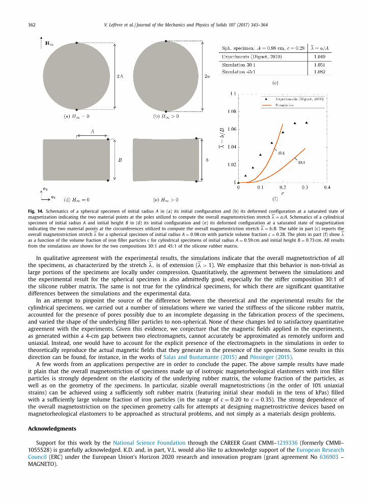
362 V. Lefèvre et al. / Journal of the Mechanics and Physics of Solids 107 (2017) 343–364

Fig. 14. Schematics of a spherical specimen of initial radius A in (a) its initial configuration and (b) its deformed configuration at a saturated state of

magnetization indicating the two material points at the poles utilized to compute the overall magnetostriction stretch λ = a/A . Schematics of a cylindrical

specimen of initial radius A and initial height B in (d) its initial configuration and (e) its deformed configuration at a saturated state of magnetization

indicating the two material points at the circumferences utilized to compute the overall magnetostriction stretch λ = b/B . The table in part (c) reports the

overall magnetostriction stretch λ for a spherical specimen of initial radius A = 0 . 98 cm with particle volume fraction c = 0 . 28 . The plots in part (f) show λ

as a function of the volume fraction of iron filler particles c for cylindrical specimens of initial radius A = 0 . 59 cm and initial height B = 0 . 73 cm. All results

from the simulations are shown for the two compositions 30:1 and 45:1 of the silicone rubber matrix.

In qualitative agreement with the experimental results, the simulations indicate that the overall magnetostriction of all

the specimens, as characterized by the stretch λ, is of extension ( λ > 1 ). We emphasize that this behavior is non-trivial as

large portions of the specimens are locally under compression. Quantitatively, the agreement between the simulations and

the experimental result for the spherical specimen is also admittedly good, especially for the stiffer composition 30:1 of

the silicone rubber matrix. The same is not true for the cylindrical specimens, for which there are significant quantitative

differences between the simulations and the experimental data.

In an attempt to pinpoint the source of the difference between the theoretical and the experimental results for the

cylindrical specimens, we carried out a number of simulations where we varied the stiffness of the silicone rubber matrix,

accounted for the presence of pores possibly due to an incomplete degassing in the fabrication process of the specimens,

and varied the shape of the underlying filler particles to non-spherical. None of these changes led to satisfactory quantitative

agreement with the experiments. Given this evidence, we conjecture that the magnetic fields applied in the experiments,

as generated within a 4-cm gap between two electromagnets, cannot accurately be approximated as remotely uniform and

uniaxial. Instead, one would have to account for the explicit presence of the electromagnets in the simulations in order to

theoretically reproduce the actual magnetic fields that they generate in the presence of the specimens. Some results in this

direction can be found, for instance, in the works of Salas and Bustamante (2015) and Pössinger (2015) .

A few words from an applications perspective are in order to conclude the paper. The above sample results have made

it plain that the overall magnetostriction of specimens made up of isotropic magnetorheological elastomers with iron filler

particles is strongly dependent on the elasticity of the underlying rubber matrix, the volume fraction of the particles, as

well as on the geometry of the specimens. In particular, sizable overall magnetostrictions (in the order of 10% uniaxial

strains) can be achieved using a sufficiently soft rubber matrix (featuring initial shear moduli in the tens of kPas) filled

with a sufficiently large volume fraction of iron particles (in the range of c = 0 . 20 to c = 0 . 35 ). The strong dependence of

the overall magnetostriction on the specimen geometry calls for attempts at designing magnetrostrictive devices based on

magnetorheological elastomers to be approached as structural problems, and not simply as a materials design problems.

Acknowledgments

Support for this work by the National Science Foundation through the CAREER Grant CMMI–1219336 (formerly CMMI–

1055528) is gratefully acknowledged. K.D. and, in part, V.L. would also like to acknowledge support of the European Research

Council (ERC) under the European Union’s Horizon 2020 research and innovation program (grant agreement No 636903 –

MAGNETO).

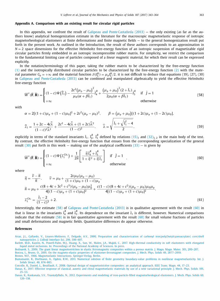
V. Lefèvre et al. / Journal of the Mechanics and Physics of Solids 107 (2017) 343–364 363

Appendix A. Comparison with an existing result for circular rigid particles

In this appendix, we confront the result of Galipeau and Ponte Castañeda (2013) — the only existing (as far as the au-

thors know) analytical homogenization estimate in the literature for the macroscopic magnetoelastic response of isotropic

magnetorheological elastomers at finite deformations and finite magnetic fields — to the general homogenization result put

forth in the present work. As outlined in the Introduction, the result of these authors corresponds to an approximation in

N = 2 space dimensions for the effective Helmholtz free-energy function of an isotropic suspension of magnetizable rigid

circular particles firmly embedded in an isotropic incompressible rubber matrix. For simplicity, we restrict the comparison

to the fundamental limiting case of particles composed of a linear magnetic material, for which their result can be expressed

explicitly.

In the notation/terminology of this paper, taking the rubber matrix to be characterized by the free-energy function

(1) and the isotropically distributed circular particles to be characterized by the free-energy function (2) with the mate-

rial parameter G p = + ∞ and the material function S(I H 5 ) = μp I

H 5

/ 2 , it is not difficult to deduce that equations (19), (27), (30)

in Galipeau and Ponte Castañeda (2013) can be combined and manipulated algebraically to yield the effective Helmholtz

free-energy function

W

∗( F , B ) =

⎧ ⎨ ⎩

(1 − c)�( I 1 )

−2 c 2 (μp − μ0

)2

μ0 (α + βI 1 ) I

B

4 +

(μp + μ0

)2 (2 + I 1 )

2 μ0 (α + βI 1 ) I

B

5 if J = 1

+ ∞ otherwise

(58)

with

α = 2[(1 + c) μp + (1 − c) μ0 ] 2 + 2 c 2 (μp − μ0 )

2 , β =

(μp + μ0

)[(1 + 2 c) μp + (1 − 2 c) μ0 ] ,

I 1 =

1 + 2 c − 4 c λ

(1 − c) 2 λ2 +

2 c 2 − 4 c λ + (1 + 2 c) λ2

(1 − c) 2 , λ =

√

I 1 +

√

I 2

1 − 4

2

, (59)

explicitly in terms of the standard invariants I 1 , I B

4 , I B

5 defined by relations (15) 1 and (32) 1, 2 in the main body of the text.

By contrast, the effective Helmholtz free-energy function that ensues from the corresponding specialization of the general

result (30) put forth in this work — making use of the analytical coefficients (33) — is given by

W

∗( F , B ) =

⎧ ⎪ ⎨ ⎪ ⎩

(1 − c)�(I Cir r

1

)+

1

2

n

[ ˜ η I B

4 + I B

5

1 +

η 2 +

η I 1

]

if J = 1

+ ∞ otherwise

, (60)

where

˜ η =

˜ ν −˜ n ˜ n

, ˜ ν = μ0 +

2 cμ0 (μp − μ0 )

(1 + c) μ0 + (1 − c) μp

,

˜ n = μ0 +

c(8 + 4 c + 3 c 2 + c 3 )(μp − μ0 ) μ2 0

4[(1 − c) μp + (1 + c) μ0 ] 2 +

c(1 − c)(8 + 4 c + c 2 )(μp − μ0 ) μ0 μp

4[(1 − c) μp + (1 + c) μ0 ] 2 ,

I Cir r 1

=

I 1 − 2

(1 − c) 3 + 2 . (61)

Interestingly, the estimate (58) of Galipeau and Ponte Castañeda (2013) is in qualitative agreement with the result (60) in

that is linear in the invariants I B

4 and I B

5 . Its dependence on the invariant I 1 is different, however. Numerical comparisons

indicate that the estimate (58) is in fair quantitative agreement with the result (60) for small volume fractions of particles

and small deformations and magnetic fields. Quantitative differences do appear otherwise.

References

Arias, J.L. , Gallardo, V. , Linares-Molinero, F. , Delgado, A.V. , 2006. Preparation and characterization of carbonyl iron/poly(butylcyanoacrylate) core/shell

nanoparticles. J. Colloid Interface Sci. 299, 599–607 . Barlett, M.D. , Kazem, N. , Powell-Palm, M.J. , Huang, X. , Sun, W. , Malen, J.A. , Majidi, C. , 2017. High-thermal conductivity in soft elastomers with elongated

liquid metal inclusions. In: Proceedings of the National Academy of Sciences . In press. Bednarek, S. , 2006. The giant linear magnetostriction in elastic ferromagnetic composites within a porous matrix. J. Magn. Magn. Mater. 301, 200–207 .

Borcea, L. , Bruno, O. , 2001. On the magneto-elastic properties of elastomer-ferromagnet composites. J. Mech. Phys. Solids 49, 2877–2919 . Brown, W.F. , 1966. Magnetoelastic Interactions. Springer-Verlag, Berlin .

Bustamante, R. , Dorfmann, A. , Ogden, R.W. , 2011. Numerical solution of finite geometry boundary-value problems in nonlinear magnetoelasticity. Int. J.

Solids Struct. 48, 874–883 . Corcolle, R. , Daniel, L. , Bouillault, F. , 2008. Optimal design of magnetostrictive composites: an analytical approach. IEEE Trans. Magn. 44, 17–23 .

Danas, K. , 2017. Effective response of classical, auxetic and chiral magnetoelastic materials by use of a new variational principle. J. Mech. Phys. Solids 105,25–53 .

Danas, K. , Kankanala, S.V. , Triantafyllidis, N. , 2012. Experiments and modeling of iron-particle-filled magnetorheological elastomers. J. Mech. Phys. Solids 60,120–138 .

364 V. Lefèvre et al. / Journal of the Mechanics and Physics of Solids 107 (2017) 343–364

Diguet, G. , 2010. Huge Magnetostriction of Magneto-Rheological Composite. Université de Grenoble. Ph.d. thesis . Diguet, G. , Beaugnon, E. , Cavaillé, J.Y. , 2009. From dipolar interactions of a random distribution of ferromagnetic particles to magnetostriction. J. Magn.

Magn. Mater. 321, 396–401 . Diguet, G. , Beaugnon, E. , Cavaillé, J.Y. , 2010. Shape effect in the magnetostriction of ferromagnetic composite. J. Magn. Magn. Mater. 322, 3337–3341 .

Dorfmann, A. , Ogden, R.W. , 2004. Nonlinear magnetoelastic deformations. Q. J. Mech. Appl. Math. 57, 599–622 . Dorfmann, A. , Ogden, R.W. , 2005. Some problems in nonlinear magnetoelasticity. Z. angew. Math. Phys. 56, 718–745 .

Galipeau, E. , Ponte Castaeda, P. , 2012. The effect of particle shape and distribution on the macroscopic behavior of magnetoelastic composites. Int. J. Solids

Struct. 49, 1–17 . Galipeau, E. , Ponte Castañeda, P. , 2013. A finite-strain constitutive model for magnetorheological elastomers: magnetic torques and fiber rotations. J. Mech.

Phys. Solids 61, 1065–1090 . Galipeau, E. , Rudykh, S. , deBotton, G. , Ponte Castañeda, P. , 2014. Magnetoactive elastomers with periodic and random microstructures. Int. J. Solids Struct.

51, 3012–3024 . Ge, L. , Gong, X. , Fan, Y. , Xuan, S. , 2013. Preparation and mechanical properties of the magnetorheological elastomer based on natural rubber/rosin glycerin

hybrid matrix. Smart Mater. Struct. 22, 115029 . Gent, A.N. , 1996. A new constitutive relation for rubber. Rubber Chem. Technol. 69, 59–61 .

Ginder, J.M. , Nichols, M.E. , Elie, L.D. , Tardi, J.L. , 1999. Magnetorheological elastomers: properties and application. In: Proceedings SPIE 3675, Smart Structures

and Materials 1999: Smart Materials Technologies, pp. 131–138 . Guan, X. , Dong, X. , Ou, J. , 2008. Magnetostrictive effect of magnetorheological elastomer. J. Magn. Magn. Mater. 320, 158–163 .

Ivanov, A.O. , Kantorovich, S.S. , Reznikov, E.N. , Holm, C. , Pshenichnikov, A.F. , Lebedev, A.V. , Chremos, A. , Camp, P.J. , 2007. Magnetic properties of polydisperseferrofluids: a critical comparison between experiment, theory, and computer simulation. Phys. Rev. E 75, 1–12 .

Javili, A. , Chatzigeorgiou, G. , Steinmann, P. , 2013. Computational homogenization in magneto-mechanics. Int. J. Solids Struct. 50, 4197–4216 . Jolly, M.R. , Carlson, J.D. , Muñoz, B.C. , Bullions, T.A. , 1996. The magnetoviscoelastic effect of elastomer composites consisting of ferrous particles embedded

in a polymer matrix. J. Intell. Mater. Syst. Struct. 7, 613–622 .

Ju, B.X. , Yu, M. , Fu, J. , Yang, Q. , Liu, X.Q. , Zheng, X. , 2012. A novel porous magnetorheological elastomer: preparation and evaluation. Smart Mater. Struct. 21,035001 .

Kalina, K.A. , Metsch, P. , Kästner, M. , 2016. Microscale modeling and simulation of magnetorheological elastomers at finite strains: a study on the influenceof mechanical preloads. Int. J. Solids Struct. 102–103, 286–296 .

Kankanala, S.V. , Triantafyllidis, N. , 2004. On finitely strained magnetorheological elastomers. J. Mech. Phys. Solids 52, 2869–2908 . Keip, M.A. , Rambausek, M. , 2016. A multiscale approach to the computational characterization of magnetorheological elastomers. Int. J. Numer. Meth. Eng.

107, 338–360 .

Lefèvre, V. , Lopez-Pamies, O. , 2014. The overall elastic dielectric properties of a suspension of spherical particles in rubber: an exact explicit solution in thesmall-deformation limit. J. App. Phys. 116, 134106 .

Lefèvre, V. , Lopez-Pamies, O. , 2015. The overall elastic dielectric properties of fiber-strengthened/weakened elastomers. J. Appl. Mech. 82, 111009 . Lefèvre, V. , Lopez-Pamies, O. , 2017a. Nonlinear electroelastic deformations of dielectric elastomer composites: I — ideal elastic dielectrics. J. Mech. Phys.

Solids 99, 409–437 . Lefèvre, V. , Lopez-Pamies, O. , 2017b. Nonlinear electroelastic deformations of dielectric elastomer composites: II — non-gaussian elastic dielectrics. J. Mech.

Phys. Solids 99, 438–470 .

Liu, L.P. , James, R.D. , Leo, P.H. , 2006. Magnetostrictive composites in the dilute limit. J. Mech. Phys. Solids 54, 951–974 . Lopez-Lopez, M.T. , Kuzhir, P. , Lacis, S. , Bossis, G. , Gonzalez-Caballero, F. , Duran, J.D.G. , 2006. Magnetorheology for suspensions of solid particles dispersed in

ferrofluids. J. Phys. Condens. Matter 18, 2803–2813 . Lopez-Pamies, O. , 2014. Elastic dielectric composites: theory and application to particle-filled ideal dielectrics. J. Mech. Phys. Solids 64, 61–82 .

Lopez-Pamies, O. , 2010. A new i 1 -based hyperelastic model for rubber elastic materials. C. R. Mec. 338, 3–11 . 2010. Lopez-Pamies, O. , Ponte Castañeda, P. , 2006. On the overall behavior, microstructure evolution, and macroscopic stability in reinforced rubbers at large

deformations: II — application to cylindrical fibers. J. Mech. Phys. Solids 54, 831–863 .

Miehe, C. , Vallicotti, D. , Teichtmeister, S. , 2016. Homogenization and multiscale stability analysis in finite magneto-electro-elasticity. application to softmatter EE, ME and MEE composites. Comput. Methods Appl. Mech. Eng. 300, 294–346 .

Nunes, L.C.S. , Moreira, D.C. , 2013. Simple shear under large deformation: experimental and theoretical analyses. Eur. J. Mech. A-Solids 42, 315–322 . Pelteret, J.-P. , Davydov, D. , McBride, A. , Vu, D.K. , Steinmann, P. , 2016. Computational electro-elasticity and magneto-elasticity for quasi-incompressible media

immersed in free space. Int. J. Numer. Methods Eng. 108, 307–1342 . Ponte Castañeda, P. , Galipeau, E. , 2011. Homogenization-based constitutive models for magnetorheological elastomers at finite strain. J. Mech. Phys. Solids

59, 194–215 .

Pössinger, T. , 2015. Experimental Characterization, Modeling and Simulation of Magneto-Rheological Elastomers. Ecole Polytechnique. Ph.d. thesis . Poulain, X. , Lefèvre, V. , Lopez-Pamies, O. , Ravi-Chandar, K. , 2017. Damage in elastomers: nucleation and growth of cavities, micro-cracks, and macro-cracks.

Int. J. Fracture 205, 1–21 . Ritto, T.G. , Nunes, L.C.S. , 2015. Bayesian model selection of hyperelastic models for simple and pure shear at large deformations. Comput. Struct. 156,

101–109 . Salas, E. , Bustamante, R. , 2015. Numerical solution of some boundary value problems in nonlinear magneto-elasticity. J. Intell. Mater. Syst. Struct. 26,

156–171 . Saxena, S.A. , Pelteret, J.-P. , Steinmann, P. , 2015. Modelling of iron-filled magneto-active polymers with a dispersed chain-like microstructure. Eur. J. Mech.

A-Solids 50, 132–151 .

Shiga, T. , Okada, A. , Kurauchi, T. , 1995. Magnetoviscoelastic behavior of composite gels. J. Appl. Polym. Sci. 58, 787–792 . Spinelli, S.A. , Lefèvre, V. , Lopez-Pamies, O. , 2015. Dielectric elastomer composites: a general closed-form solution in the small-deformation limit. J. Mech.

Phys. Solids 83, 263–284 . Stratton, J.S. , 1941. Electromagnetic Theory. McGraw-Hill .

Tian, L. , Tevet-Deree, L. , deBotton, G. , Bhattacharya, K. , 2012. Dielectric elastomer composites. J. Mech. Phys. Solids 60, 181–198 . Varga, Z. , Filipcsei, G. , Zrínyi, M. , 2005. Smart composites with controlled anisotropy. Polymer 46, 7779–7787 .

Wang, X. , Gordaninejad, F. , 2009. A new magnetorheological fluid-elastomer mount: phenomenological modeling and experimental study. Smart Mater.

Struct. 18, 095045 . Wang, Y. , Hu, Y. , Chen, L. , Gong, X. , Jiang, W. , Zhang, P. , Chen, Z. , 2006. Effects of rubber/magnetic particle interactions on the performance of magnetorhe-

ological elastomers. Polymer Testing 25, 262–267 . Zhou, Y. , Shin, F.G. , 2005. Modeling of magnetostriction in particulate composite materials. IEEE Trans. Magn. 41, 2071–2076 .