1

Can FTAA suspend the law of gravity and give the Americas higher growthand better income distributions?

Bernardo Blum and Edward E. LeamerToronto and UCLA

I. Introduction

In this paper we explore three related ideas:

1. The export sector is the fundamental source of both wealth and inequality: You are what you export.Exporting manufactures has been essential for high incomes and low levels of inequality. Exportingcrops and raw materials comes with low incomes and unequal income distributions.

2. The mix of exports is determined by three fundamentals: Resources, Remoteness, and Climate.Manufacturing likes cool climates, an educated workforce, and locations close to the high-wagemarketplaces of Europe and North-America.

3. The volume of exports and the wealth formation that comes from the export sector can be impeded byinward looking, isolationist policies. Governments can affect the export mix only slightly and mostlythrough policies that alter the effects of the fundamental drivers, for example, by encouraging theformation of institutions that make a country effectively closer to global marketplaces.

With this as a framework, the Free Trade Area of the Americas (FTAA) agreement can have two effects. Itcan set free the fundamental determinants of exports (resources, location and climate) and allow theparticipating countries to become “all they are capable of being.” This is not necessarily entirely goodnews for Latin America, whose abundant resources, far-away locations and tropical climates tend tosupport relatively low per capita incomes and unequal income distributions. But, more optimistically, theFTAA may also bring Latin America closer to global GDP, both by supporting higher per capita GDPs inthe region (thus lifting the region by its own bootstraps), and also by the creation of institutions that havethe effect of making Latin America closer to the high-wage marketplaces of North America.

The first part of this paper presents our view about the fundamental determinants of wealth and inequality.In the second part we assemble a body of evidence, much of which suggests that far-away resource-abundant tropical countries have great difficulties attracting manufacturing activities, other than mundaneand labor-intensive tasks like sewing hems on t-shirts. Communities that cannot attract the human-capital-intensive tasks in manufacturing or the human-capital-intensive tasks in the services of the post-industrialage (e.g. digital entertainment and financial management and business consulting) are destined to have lowper capita incomes and uncomfortable levels of inequality.

To assemble the evidence, we have cast our data net broadly, and use a comprehensive dataset includingdata on countries’ trade, outputs, inequality, production resources, climate, and location. Finally, in thethird section, we use the framework and the evidence to offer an opinion regarding what impacts the FreeTrade Area of the Americas agreement may have on export patterns, income, and inequality in the region.

We find in the data considerable support for the idea that exports are symptoms of the process of wealthaccumulation and distribution. Exporters of machinery and chemicals tend to have high per capita incomeswhile exporters of tropical agriculture have per capita incomes that are on average more than 80% lower.Moreover, because exporters of machinery and chemicals have a large fraction of their wealth invested inhuman capital, their incomes are generally equally distributed, while exporters of agriculture and naturalresources have incomes that are quite concentrated.

The data also support the idea that location, resources, and climates are key exogenous determinants of theexport composition of the countries. Capital intensive manufacturing activities, for example, are notperformed in hot climates or in remote parts of the globe.

2

We thus offer a fundamental explanation for the economic dilemma facing the region. With respect to thepossible effects of the FTAA agreement on incomes and inequality, our analyses indicate that a substantialimpact should not be expected. Even though the removal of the existing trade impediments should bring theregion “closer” to the world markets, most of the countries in the region will still be too far away to be ableto perform the complex tasks that are associated with high incomes and equality, not to mention that theagreement will have no impact on climates.

We are certainly not the first to propose a link between physical geography and economic development.References about such a possibility date back at least to Machiavelli (1519). Gallup, Sachs, and Mellinger(1998) indicate four major areas where it’s been suggested that physical geography may have a directimpact on economic productivity: transport cost, human health, agricultural productivity, and proximityand ownership of natural resources. In that paper, as well as in Sachs (2001), empirical evidence isprovided supporting that geography indeed has direct, as well as indirect, effects on economicdevelopment. Hall and Jones (1999) and Engerman and Sokoloff (1997) propose additional ways thatphysical geography may affect economic development by shaping the countries’ institutions. Acemoglu,Johnson, and Robinson (2001), Rodrik, Subramanian, and Trebbi (2002) and Easterly and Levine (2002) goone step further suggesting that once controlled for the effects through institutions geography has no directimpact on economic development. However, McArthur and Sachs (2001) show that the results inAcemoglu et al. (2001) are not robust to increases in the sample of countries used in the analyses.

This literature misses, we suggest, the two primary mechanisms that make geography so important. First,as explained in Leamer(2001), the fixed costs of expensive capital equipment need to be covered byoperating the equipment at high pace for long hours. This creates a distinct disadvantage for the tropics.Second, as explained in Leamer and Storper (2001), the exchange of complex uncodifiable messages canonly be done on a face-to-face basis with the participants within a handshake of each other. Vastimprovements in transportation and communication technologies over the last half century, which mighthave rendered geography less relevant, have not done so, since these technologies have not improved thelong-distance exchange of ideas and commitments. Thus the production of the ideas and the production ofthe new products remain tightly clustered, leaving much of manufacturing firmly “rooted” where it is, inthe United States and Europe. Apparel and footwear are footloose. Machinery and pharmaceuticals arenot.1

II. A view about the process of wealth creation anddistribution

A. Exports are the most important source of wealth andinequality

Wealth is primarily generated by exports. This isn't true for the globe overall, since so far the Moon hasbeen a recipient of very few exports. It is very true for individuals in advanced developed countries, who,because of a very fine division of labor, "export" almost 100% of what they produce. (How mucheconomics does an economics professor consume?) Between the globe and the individual are very fewlarge countries, which, like the globe overall, experience internally driven growth. A prominent example isthe United States during the Internet Rush from 1997 to 2000, with growth driven internally by a mad dash

1 Our paper is also related but different than the so called “New Geography” literature summarized inFujita, Krugman, and Venables (1999). This literature deals with how increasing returns to scale,agglomeration economies, transport costs, and product differentiation can affect the way economic activityis spatially organized, even when physical geography is undifferentiated. Even though recent developmentsby Strauss-Kahn (2001), Venables and Limao (2002), and Redding and Schott (2002) incorporate somephysical geography into the picture the mechanisms we suggest are very different.

3

for the Web. But most countries are more like individuals than the globe. Their production structures arespecialized and their growth comes from expanding efficiently the activities they are good at, and exportingthe surplus to the rest of the world.

Compensation for various kinds of inputs varies greatly depending on the export mix. Raw labor powerand human capital are widely owned, but where human capital is poorly rewarded compared with othercapital assets, ownership of the most important productive inputs tends to be concentrated on the few.Thus: Find out what a community exports and why, and you are 90% of the way toward understanding itsper capita income and its degree inequality.

Table 1 offers a classification of exports that is intended to capture our ideas about wealth and inequality.The table identifies eight different categories of exports in which communities might specialize, and thekinds of capital and other assets needed to produce these items. There are five broad groups ofproducts/services: (a) products made with raw labor only; (b) primary products and crops, (c) distributionservices, (d) manufactures, and (e) intellectual services. The inputs needed to produce these items fall intothe usual three broad categories of land, labor and capital. The raw labor inputs are physical and mentalexertions. Capital takes the form of equipment, skills, knowledge, experience, reputation and humannetworks, the latter being critical inputs into the activities of distribution, finance and the creation of ideasand content (think Hollywood). Land includes the usual mineral resources and fertile cropland, but alsolocation (closeness to sources of inputs and closeness to markets).

The last two columns indicate the level of incomes and inequality that are typically associated withcommunities that specialize in these activities. Inequality is determined largely by the ownership of theproductive inputs. Of these assets, it is only the human skills created by training that are broadly ownedand it is only those communities with economies heavily skill-based that have equal incomes. That meansmanufacturing. In contrast, land, physical capital, and human ability are assets with concentratedownership. Thus countries that export primary products and crops and ideas and content have unequalincomes.

4

Table 1 Export Classifications

A Classification of Economies by their principal exports

Export Group Export Example CapitalAssets

OtherAssets

Incomes Inequality

Products of UnskilledLabor

1 Handmade goods Handicrafts, hand-made textiles

None Low Low

Natural Resource Based Primary Products and Crops2 Raw materials and

cropsCoffee beans, logs Permanent

Crops,Equipment

Land Low High

Distribution3 Distribution Services Shipping,

warehousingDistributionNetworks,infrastructure

Location Moderate Moderate

Manufacturing and Food/Resource Processing4 Footloose

manufacturingApparel, footwear Equipment, Skills Medium Low

5 Processing Food products,lumber, paper

Equipment,Skills

Closenessto inputs

Medium Low

6 Noncodifiablemanufactures

Pharmaceuticals Equipment,Knowledge

Agglomerations

High Moderate

Intellectual Services

7 Financial Services Investment Banking TrustNetworks

Instincts High Moderate

8 Ideas and Content R&D, entertainment,marketing, design

Experience,Reputation,IdeaNetworks

Ability High High

5

B. Wealth and inequality in resource-based, industrial, andpost-industrial communities.

In the schema in Table 1, natural resources support three kinds of activities: (a) extracting/growing, (b)processing and (c) distribution. In the extracting/growing economies, capital is embodied in permanentcrops (coffee plantations), in cleared, irrigated and otherwise improved land, in transportation systems, andin housing. These activities require very little human capital, and wealth comes from an abundance ofnatural resources. Then income inequality is determined by the distribution of ownership of the naturalresources, which is usually very unequal. Human capital plays a greater role at distribution centers andprocessing locations, which often are close to the natural resource. At these distribution locations, incomesare often higher and more equally distributed.

Global trade prior to the industrial revolution was mostly the exchange of handicrafts, raw materials,foodstuffs and distribution services. With the dawn of the industrial age, the nature of global trade shiftedto manufactured products, led by textiles and footwear and apparel. While much of manufacturing capitaleven at the beginning of the 20th Century was structures, the shift in favor of equipment has been verysubstantial. In the investment boom of the 1990s, the ratio of investment in producer durables and softwarerelative to structures rose to a record high of 3-to-1.

The operation of the equipment requires human capital, and most capital in the industrial communities isembodied in equipment and humans skills. Ownership of the equipment can be and often is highlyconcentrated, just as the ownership of natural resources. Ownership of human skills, however, by itsessential nature, is necessarily broad. The equipment of the industrial age, like a forklift, requires trainableskills that depend very little on native ability. Thus on the factory floor the return on human capitalinvestment is high and pretty much the same for everyone.

If it doesn’t matter much who operates a forklift, it matters greatly who types on a computer keyboard.Thus like the industrial age, the post-industrial age has services produced with a combination of equipment(recording studios) and human capital (singing skills). While manufacturing requires trainable skills, thepost-industrial activities of finance and innovation require knowledge and understanding. Unlike theindustrial age, in the post-industrial age the rate of return to investments in human capital varies greatlyfrom individual to individual. (You cannot teach me to sing, I am sorry.) This brings with it aconcentration of capital in the hands of the few and inequality levels that are reminiscent of the pre-industrial age.

C. In the Industrial Age, wealth has come especially fromexporting manufactures

Not all countries are equally well suited to compete in manufacturing, and some countries in the industrialage remain as suppliers of raw materials and foodstuffs. These activities have not been technologicallystagnant. On the contrary, both agriculture and resource extraction have experienced an increase inmechanization that closely parallels progress in manufacturing.

Mechanization of agriculture and raw material extraction is similar but also different from mechanizationof manufacturing activities. It is similar in the sense that it puts into the hands of workers expensiveequipment that needs to be operated for long hours at high pace to cover the capital costs. This createshigh-effort high-wage opportunities for workers with some formal education. It is similar in the sense thatit lowers the labor to output ratio. The difference is that agriculture and resource extraction have a fixedinput: land. Mechanization lowers the worker to land ratio and thus reduces the number of jobs inagriculture. In manufacturing the number of jobs can be maintained or even increased in the face ofincreased mechanization provided that manufacturing can attract the needed amount of capital.

6

For example, the United States experienced a sharp drop in its agricultural workforce over the 20th Centurybut an increase in its manufacturing workforce. In 1900, 10 million agricultural workers comprised 40% ofthe workers. In 1970, only 4 million farm jobs remained comprising only 5% of the workforce.Meanwhile, manufacturing jobs increased from 5 million to 20 million, rising from 20% of the workforceto 30%.

This rise in the proportion of jobs in manufacturing cannot be explained only by the absence of a fixedfactor, since consumers, facing a fixed set of products must eventually become satiated: how many horse-drawn carriages can you possibly desire? With a fixed product mix the return on capital in manufacturingwould have surely fallen to a level too low to attract more investment, and jobs would have expandedinstead in services. If we today had the same mix of products as in 1900 – no automobiles, or refrigerators,no televisions, no personal computers, etc., etc. - we surely would have a much smaller global workforcein manufacturing. But the 20th Century has experienced wondrous product innovation that has paralleledthe process innovation. Thus the fundamental reason for the expansion of the global manufacturing jobs inthe first seven decades of the 20th Century has been product innovation.

The difference between agriculture and manufacturing should alarm exporters of natural resource basedproducts, processed or otherwise. Countries that cannot attract manufacturing activities face the verydifficult problem of how to find work both for the new entrants into the labor force and also for the naturalresource workers who are inevitably displaced by mechanization.

7

D. Manufacturing is done in cold climate, close to marketsand separated from agriculture

The ability of a country to attract manufacturing is determined by three features:

1. Resources2. Location3. Climate

Manufacturing prefers cold climates where equipment can be operated without breakdowns at high pace forlong hours during the day. Manufacturing seeks stable real exchange rates and an educated workforce,neither of which are offered by natural resource rich countries. And many manufacturing activities preferto cluster next to like activities and close to the high-wage markets of North America and Europe andJapan.

1. The transition from pre-industrial to industrial isdifficult for natural resource rich countries

The conceptual framework that we use for thinking about these issues is a three-factor (land ,labor andcapital), multi-good, Heckscher-Ohlin model with variable effort levels which looks like technologicaldifferences. This framework suggests that abundance of natural resources is helpful in the pre-industrialage but can be a hindrance toward progress in the industrial age. Natural resource rich communities investtheir scarce savings mostly in improvements in land, in permanent crops, and extractive equipment andvery little in human capital, which has a very low return on a coffee plantation or the equivalent. Thiscreates a barrier to development since once the resource is fully developed and further wealth accumulationcould come only from growing manufacturing, the educational system may not be ready to prepare theworkforce for jobs on the factory floor. Equipment may then seek workers in other communities that havethe literacy skills and work ethics needed in the command-and-control hierarchical organizations that leadthe global competition in manufacturing.

There are some notable exceptions to the hindering effects of natural resources in the northern regions ofEurope (Finland and Sweden) and North America (Canada). The comparison between Latin America andthese northern softwood producers may not be completely meaningful. Softwood logs are different fromcoffee, since wood processing can extend from sawing to the much more human and physical-capitalintensive operations in pulp and paper. Food processing is more limited in scope and may not supportextensive investment in human capital. Secondly, as we will argue more below, manufacturing likes coldweather, which is in abundant supply in Canada, Finland and Sweden, but very scarce in Latin America.Also, these softwood producers may be different from Latin American countries with regard to humancapital formation, since these northern countries may have made a heavy commitment to broad humancapital accumulation for non-economic reasons prior to the period when the private rate of return to humancapital exceeded the private rate of return to physical capital. Furthermore, these softwood producers sitright on top of the attractive markets in Europe and North America, while Latin America is far away. Forthat reason, and others, educational investments may not have a sure payoff. Indeed, Argentina, a formerlywealthy natural resources exporter still had substantial measured human capital accumulation, butnonetheless did not manage to make the transition to an industrial economy,.

8

2. Climate: equipment doesn’t like hot humid areas.

The shift from the Agrarian Age to the Industrial Age came with a movement of wealth creation from theMediterranean climates to cooler climes, for two reasons. First, there is a fundamental difference in thetechnology of agricultural production and the technology of manufacturing. A field can be tended bymany or by few, and adding another worker doesn’t affect the productivity of the others. Two lazyworkers equal one productive worker. But a machine can be tended by only one worker. The output of amachine at the end of the day depends on the speed of work, and the attentiveness of the worker. Theowner of a farm doesn’t much care if there are a few unproductive workers or one productive worker– theycan be paid on a piece rate system - since in the end the land commands the same rent. But the owner ofan expensive machine cannot use a piece rate system because a lazy worker may not produce enoughoutput to cover the cost of the machine.. (See Leamer(1999))

The need to spread the fixed cost of capital over a large labor input makes industrial equipment andfactories seek climates in which the equipment can be operated for long hours during the day at highspeeds. The problems confronting manufacturing in the tropics are many. Human effort and attentivenessare hard to maintain for extended periods of time in hot and humid climates, and machines break downmore frequently. It is only with the advent of air-conditioning that manufacturers started moving “south”in search of low wages, but in these hot and humid climates workers must, in effect, rent the equipment,and pay the added capital costs for the air-conditioning, and the marginal operating costs as well. Thiskeeps a permanent gap between wages in the “North” and wages in the “South.”

3. Location: communication of complex ideas requiresface-to-face meetings

Both the industrial age and the post-industrial age require workers to master complex new tasks that thenew equipment and new products demand. Leamer and Storper(2001) argue that this human capital iscreated only by close human interactions (watching the master), a communication technology whichdictates the geographic concentration of innovative manufacturing. While great improvements intransportation and communication technologies have made it much cheaper to transport goods andcodifiable messages, these technologies help very little in the transshipment of uncodifiable knowledge.Only when products mature and become standardized can the knowledge of how to produce them becodified in words and blueprints and sent to remote locations where the products can successfully be made.The productive activities at these remote locations tend toward the mundane and the repetitive, and thusrequire much less human capital than the innovative activities done at the great centers of both theindustrial and post-industrial ages. Without broadly owned human capital, these remote locations mayhave greater inequality than the centers of the industrial age.

4. Location: Enforcement of contracts is best done inclose proximity

In addition to allowing the transfer of complex messages, closeness can be important for the maintenanceof guarantees. "Search" goods whose value is transparent from a single inspection can be exchangedthrough long-distance and faceless transactions. But "experience" goods have value that is revealed onlythrough years of use, and it is essential for the buyer to be able to find the seller in the event that theproduct does not live up to its explicit or implicit guarantees.

9

III. Data evidenceWithin the time and space limits of this paper, we cannot provide compelling evidence in support of allthese ideas, but we can offer some significant support for many.

A. The link between exports, incomes, and inequalitySubstantial evidence of “you are what you export” comes in the form of a clustering of countries in termsof their export patterns, and then computing how the average per capita GDPs and average GINIs differbetween the clusters. We find, among other things, that exporters of tropical agricultural products havelower per capita GDPs and high GINIs.

Next we report some simple regressions that include more than one export product and also remoteness andtrade dependence. Even in this horse race between competing explanations, exporting tropical agriculturalproducts contributes to low per capita GDPs and unequal incomes. After controlling for export mix, beingfar away doesn’t seem to affect GDP per capita but it does contribute to higher GINIs.

1. Clustering of Countries 1987In Table 2 we report two groups of countries based on their export shares, first exporters of tropicalagricultural products and second exporters of (footloose) labor-intensive manufactures2. Exporters oftropical agriculture products rarely export other goods, especially not manufacturing. In contrast, theheterogeneity within the group of exporters of labor intensive manufactures is the largest among any ofthe groups (except the mixed comparative advantage group that is precisely defined based on itsheterogeneity). Interestingly there are countries in this group that also export capital intensive manufacturesor machinery, but at the same time there are tropical agriculture exporters.

2 There are nine clusters in all. See the website at WWW for more details.

10

Table 2: Two Clusters of Countries: Exports / Total TradePet R. Mat. For Trop. Ag. Anl. Cer. Lab Cap Mach. Chem.

MDG 0 0.03 0 0.39 0.09 0.02 0.01 0.03 0 0.01HND 0 0 0.03 0.38 0.05 0.01 0.01 0 0 0TZA 0.01 0 0.01 0.28 0.01 0.13 0.01 0.02 0 0CRI 0 0 0.01 0.27 0.06 0.01 0.04 0.03 0.01 0.02FJI 0.05 0 0.03 0.27 0.04 0.01 0.03 0.02 0.02 0GTM 0.01 0 0.01 0.25 0.02 0.03 0.02 0.03 0 0.04SLV 0.01 0.01 0.01 0.25 0.02 0.02 0.02 0.03 0.01 0.03GHA 0.01 0.14 0.07 0.23 0.02 0 0.03 0 0 0COL 0.15 0.03 0.01 0.23 0.02 0.01 0.06 0.02 0.01 0.02ECU 0.2 0 0.01 0.17 0.12 0.01 0.01 0 0 0LKA 0.02 0 0 0.16 0.01 0.01 0.17 0.02 0.01 0ETH 0.01 0 0 0.15 0.07 0.01 0 0 0 0CMR 0.06 0.02 0.04 0.13 0.01 0.02 0.01 0.01 0.03 0.01

HKG 0 0.01 0.01 0.01 0.01 0.01 0.22 0.14 0.11 0.02ISR 0 0.01 0 0.03 0.01 0.01 0.16 0.07 0.08 0.06DOM 0 0 0 0.09 0.01 0.02 0.15 0.06 0.02 0PRT 0.01 0 0.06 0.02 0.01 0.01 0.15 0.06 0.07 0.02IND 0.02 0.02 0 0.05 0.03 0.03 0.15 0.1 0.03 0.02MLT 0.01 0 0 0 0 0.01 0.14 0.06 0.1 0.01THA 0 0.01 0.01 0.1 0.06 0.06 0.14 0.05 0.05 0.01PHL 0.01 0.05 0.03 0.06 0.03 0.05 0.13 0.03 0.11 0.02TUN 0.09 0.01 0 0.02 0.02 0.02 0.12 0.03 0.03 0.08TUR 0.01 0.02 0.01 0.06 0.02 0.03 0.11 0.09 0.05 0.03GRC 0.02 0.02 0 0.05 0.01 0.05 0.09 0.06 0.01 0.01

Labor Intensive Manufactures

Tropical Agriculture Products

11

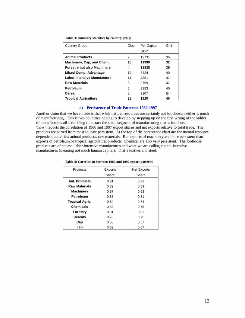
Now that we know what they export, what are they like? Is it true that “you are what you export”? Table 3reports average per capita GDPs and average GINIs for each of these groups of countries. These are sortedby per capita GDP. At the top with high per capita GDPs and low GINIs are exporters of animal productsand exporters of machinery and chemicals. At the other end with low per capita GDPs and unequalincomes are the exporters of tropical agricultural products and cereals, and petroleum and raw materials.Exporting labor-intensive manufactures helps some, but not very much. .

12

Table 3: summary statistics by country group

Country Group Obs. Per Capita Gini

GDP

Animal Products 2 12731 36Machinery, Cap, and Chem. 10 11999 32Forestry but also Machinery 4 11838 35Mixed Comp. Advantage 12 6424 40Labor Intensive Manufacture 11 4851 41Raw Materials 8 3759 47

Petroleum 6 3353 40Cereal 2 3107 54Tropical Agriculture 13 1820 46

a) Persistence of Trade Patterns: 1980-1997Another claim that we have made is that while natural resources are certainly not footloose, neither is muchof manufacturing. This leaves countries hoping to develop by stepping up on the first wrung of the ladderof manufactures all scrambling to attract the small segment of manufacturing that is footloose.Table 4 reports the correlation of 1980 and 1997 export shares and net exports relative to total trade. Theproducts are sorted from most to least persistent. At the top of the persistence chart are the natural resourcedependent activities: animal products, raw materials. But exports of machinery are more persistent thanexports of petroleum or tropical agricultural products. Chemical are also very persistent. The footlooseproducts are of course: labor-intensive manufactures and what we are calling capital-intensivemanufactures (meaning not much human capital). That’s textiles and steel.

Table 4: Correlation between 1980 and 1997 export patterns

Products Exports Net Exports

Share Share

Anl. Products 0.91 0.91Raw Materials 0.89 0.89

Machinery 0.87 0.83Petroleum 0.85 0.81

Tropical Agric. 0.84 0.84Chemicals 0.82 0.75Forestry 0.81 0.83Cereals 0.78 0.75

Cap 0.58 0.57Lab 0.32 0.37

14

2. Multiple Regressions: 1987Table 5 reports multiple regressions that explain inequality and GDP per capita in terms of export mix (netexports as a share of total trade), trade dependence and remoteness. The choice of exports comes fromtrimming out insignificant predictors. This leaves two important trade determinants of income andinequality: machinery and chemicals, good, tropical agriculture, bad.

After controlling for the product mix, trade dependence doesn’t matter and remoteness is bad for inequalitybut doesn’t much affect income levels.

The bottom line here is that 60% of the variability across countries in GDP per capita can be explained bytrade composition alone. Inequality, as measured by GINIs, is harder to predict, but exporting tropicalagricultural products seems undeniably associated with unequal incomes.

Table 5: Joint effects of exports patterns and remoteness

Inequality GDP per capita

Variable

Net Exports of Trop. Agriculture 35.44 -11403

(3.25) (-2.5)Net Exports of Machinery -17.95 8182

(-1.92) (2.0)Net Exports of Chemicals 16.21 55354

(0.44) (3.5)Remoteness 0.001 -0.2

(3.13) (-0.9)Trade dependence -1.53 1704

(-0.61) (1.5)Constant 31.1 9896

(11.46) (8.4)

R-Squared 0.48 0.6

B. What determines exports? Resources, Climate and Location.Given the stability of export patterns and the undeniable correlation between these and incomes andinequality we turn next to the empirical evidence relating exports to their underlying determinants:resources, location, and climate.

1. Location

The gravity model has often been used to study the choice of trade partners but less often the compositionof trade, although an exception is Leamer(1997). Table 6 reports the distance component of a gravity modelapplicable to each of our ten trade aggregates. This shows the distance effect on countries’ bilateral tradein different products for 136 countries in 5 different years. Except for the dummy variables the equationswere estimated in logs and included the GDP of the countries, a dummy for pairs of countries that speak thesame language, and a dummy for pairs of countries that share a common border, in addition to the distanceseparating them in kilometers.

15

Table 6 has two important messages. First, distance affects different goods differently. Cereals, tropicalagriculture, animal products, and raw materials are the least affected by distance while trade in forestproducts, petroleum, and manufacturing goods are heavily hurt by distance. Even footloose labor-intensivemanufactures has a large negative distance elasticity. Not so footloose after all.

The second message of Table 6 is that the distance effects do not seem to be fading away over time as“globalization” enthusiasts and opponents suggest. For every one of the products in the sample the effectsof distance have increased, if anything, from 1982 to 1997.

The substantial and persistent distance effect on manufactures is evidence of one of our important points:any manufacturing that involves complex uncodifiable tasks including the customization of equipment andinputs has a powerful hysteresis effect: it ain’t going anywhere.

Table 6: Distance Elasticity from Gravity Equation

Variable / Year 1982 1987 1992 1997

Petroleum -1.26(0.07)

-1.13(.06)

-1.26(.06)

-1.33(.05)

Raw Materials -.88(.04)

-.77(.04)

-.96(.04)

-1.05(.04)

Forest Products -1.08(.03)

-1.05(.04)

-1.23(.03)

-1.36(.03)

Tropical Agriculture -.70(.04)

-.66(.03)

-.82(.03)

-.82(.03)

Animal Products -.73(.04)

-.77(.04)

-.86(.03)

-.81(.03)

Cereals -.62(.04)

-.63(.04)

-.79(.03)

-.93(.03)

Labor Intensive Manufacture -1.09(.01)

-1.05(.03)

-1.03(.03)

-1.18(.03)

Capital Intensive Manufacture -1.06(.03)

-.99(.03)

-1.07(.03)

-1.17(.03)

Machinery -1.04(.03)

-.93(.03)

-1.00(.03)

-1.12(.03)

Chemicals -1.14(.03)

-1.18(.03)

-1.27(.03)

-1.34(.03)

* Standard Errors in parenthesis.

It seems surprising that the great rise in global trade in the last several decades has not been associated witha declining distance elasticity. It might be the case that although the marginal effects of distance on tradehave not decreased over time the average effect have. The average distance, in kilometers, 1 US$ ofdifferent products traveled in different years3 confirms that goods were not traveling longer distances in1997 that they were in 1982. Why, then, the big increase in trade compared with GDP? If the globe isn’tgetting smaller what is happening? The gravity model has the answer: GDP is getting more dispersed.The growth of trade across the Pacific comes from having more equal GDPs in North America and Asia.

3 Not shown but available online at WWW

16

2. Resources

The simple gravity model suffers from including no variables that measure comparative advantage. As aconsequence, it is possible that too much is attributed to distance. It could be that machinery and chemicalsare produced close to markets and tropical agriculture produced in remote areas just because the globaldistribution of endowments dictates so. Next we deal with both resources and distance at the same time.

The descriptive model that drives this two-step estimation has potential net exports a function of resourcesP(Resources) but actual trade reduced by a gravity effect: Net Exports/Worker = PotentialTrade(Resources/Worker) * Volume Effect(distance, country size). A very rough way of estimating thismodel is reported here. Table 7 reports regressions of the absolute value of the country’s net exportsdivided by its labor force – a measure of trade dependence - on our measure of remoteness and on thecountry’s GDP a measure of market size (Sombart's Law). As expected, both market size and remotenessreduce the country’s trade dependence. We then use these estimated remoteness and GDP elasticities tocreate an adjustment factor for the net exports of the countries, scaling up the level of net exports to put allcountries on an equal footing, in terms of access and market size. The adjustment factor scales up netexports of distant and large countries and scales down the net exports of close and small countries. Theseadjusted net exports, always scaled by the country’s labor force as well, are then regressed against thecountries’ factor endowments and distance to markets. The results are reported in Table 8.

Table 7: Trade Dependence log(ABS(net Exports( i)/Labor)) in 1987

Pet. Raw For. Trop. Anl. Cereals Labor Capital Mach. Chem.Mat. Prod. Agric. Prod. Int. Manuf. Int. Manuf.

log(distance) -1.74** -1.52** -2.01** -0.77* -2.18** -1.43** -1.93** -1.76** -1.31** -1.14**log(GDP) 0.05 -0.09 -0.1 -0.19 -0.22 -0.18 -0.12 -0.23* -0.25* -0.17*Constant 18.7* 18.4* 22.6** 14.2** 26.3** 19.4** 23.1** 23.8** 21.2** 17.3**

Observations 68 68 68 68 68 68 67 68 68 67R-squared 0.26 0.14 0.28 0.08 0.25 0.18 0.27 0.27 0.2 0.19

* significant at 5%; ** significant at 1%

Table 8: Comparative advantage.

Pet. Raw For. Trop. Anl. Cereals Labor Capital Mach. Chem.Mat. Prod. Agric. Prod. Int. Manuf. Int. Manuf.

capital/labor 17360 49197 4398 1743 42674 23802 17554 -4448 -159213* -19812capital/labor ^ 2 -167423 -417918 -60420 948 -425622 -220714 -597716 357008 1445048 242139prim. educ/labor -87 203 -129 298 -1010 -93 181 -676 1070 -201sec. educ/labor -601 1133 -4 56 -702 285 1914 -1757 2566 -414terc. educ/labor -1305* -3098 469 523 3158 -685 -2683 -1066 2299 518cropland/labor 53 180 -24 19 -237 93 123 -163 102 31for land/labor -2.65 8.41 0.82 -2.16 -1.21 -1.63 -5.98 0.16 -2.79 -0.77pas land/labor -2.41 -26.02 0.52 -3.32 28.69 -7.36 -20.67 21.49 5.31 2.16energy/labor 0.23 -0.66 0.01 -0.29 -1.35 -0.45 -0.36 0.11 1.59 0.11Remoteness -0.01 0.19** 0 0.04** 0.24** 0.09** 0.01 -0.08* -0.43** -0.05**

Observations 69 69 69 69 69 69 69 69 69 69R-squared 0.22 0.28 0.05 0.29 0.47 0.35 0.08 0.17 0.44 0.32

* significant at 5%; ** significant at 1%

17

Besides the expected effects of endowments in exports, long predicted by the Heckscher-Ohlin model, Table8 shows that remoteness continues to hurt exports of capital intensive manufacture, machinery, andchemicals. Even after controlling for factor endowments as sources of comparative advantage farther awaycountries still are in disadvantage producing those goods. The opposite happens to raw materials, tropicalagriculture, and animal products where after controlling for endowments the farther away countries seem tohave comparative advantage producing it.

3. Climate

An important part of our view about wealth and inequality is that climate influences the activities a countrymay perform efficiently. It cannot be surprising that tropical agriculture requires tropical climates. That isnot the point. The point is that manufacturing, especially the most capital intensive segments, cannot beefficiently performed in hot climates.

Table 9 shows that the data lend strong support to this claim. A regression of the countries’ exports perworker against remoteness, standardized to have mean zero and unit variance, and the percentage of thepopulation in tropical, temperate, snow, and other climates indicate that indeed being in the temperate zoneis a strong predictor of being able to export manufactures.

Interestingly even after controlling for climate remoteness still hurts the possibilities of a country to exportmanufacturing, this being particularly true for chemicals, machinery, and capital intensive manufactures.

18

Table 9: Climate effects on exports per worker in manufacturing (1992).

Climate Zone Chemicals Machinery CAP LABTrop. & Subtrop. 213 568 296 304

Temperate 877** 1971** 1172** 1415**Snow -678 669 -613 -1401*Other -58 -128 -101 -114

Remoteness -314** -701** -347** -233* significant at 5%; ** significant at 1%

4. The truly exogenous determinants of incomes andinequality

The evidence presented so far states clearly that endowments, location, climate, export composition,incomes, and inequality are unequivocally linked. There is however a high degree of collinearity amongthese variables and we may find it difficult to sort out the separate effects, not to mention speak to causaldirections. However, we have been able to link the countries’ income and inequality measures with theirexogenous determinants. It is this link that will be explored when addressing the possible effects the FTAAagreement may have in the region.

Among the variables we expect to be linked to the countries’ income and inequality measures we argue thatthe following are truly exogenous to the process of wealth creation and distribution: share of area under agiven climate zone, remoteness, land endowments, and energy reserves. Table 10 shows how thesevariables affect income and inequality in the countries. These are weighted regressions with variance of theresidual assumed to be equal to the labor force, thus producing regression estimates analogous to a meanwith weights equal to the labor force. There is no constant in the equation because the climate shares addto one. Furthermore, for computing the t-statistics, the mean has been subtracted from dependent variable,and the t-values on the climate proportions test if that climate zone is unusual compared with all the others,not a test if the effect is zero. Finally, the resource variables are standardized to have mean zero andvariance one, thus allowing the coefficients on the climate variables to refer to the effect of climate on acountry with average endowments and to allow the coefficients on the resource variables to measure theeffect of a one-standard error increase. The climate variables int the table have been sorted by the climateeffect on GDP per capita and the resource variables by the resource effect. The final columns of the tableindicate climate shares of several countries to help make clear what these climate variables represent.

The GDP per capita regression has a successful R2 of 0.80 and several statistically significant findings. ForGDP per capita, the best climate zones are the cold and cool ones (snow humid and temperate humid),climates the US and Sweden "enjoy", but Brazil does not. These climates are associated with per capitaGDPs of $19,000 and $12,000. These climates support GDP per capita that are statistically higher thanaverage. In the other direction, the climates that are statistically inferior are tropical dry winter and ariddesert. Brazil has the former and Argentina the latter. These climates support GDP per capita of only$2,926 and $1,506 respectively.

Abundance of cropland contributes to GDP per capita. A one standard deviation increase in croplandincreases GDP per capita by $2898. Remoteness is not a good thing. A one standard deviation increase inremoteness reduces GDP per capita by $1,828.

The Gini regression is less successful. It has an R2 of only 0.40. But it confirms what we suspect: theclimate with tropical dry winter which yields a weak GDP per capita, also yields a high Gini coefficient. Ahighland climate is also associated with unequal incomes while ice tundra (think Canada and Norway)comes with equal incomes. While remoteness lowers per capita incomes, it doesn't increase inequality.Forestland is estimated to raise inequality. That variable does not distinguish hardwood from softwood

19

forests and may be reflecting mostly the cutting of tropical hardwoods. Indeed, as can be seen in the data itis Brazil not Sweden that has abundant forestland.

Table 10:

Weighted Regression Estimates: 1987 DataWeight = Labor .̂5t-stats on climate variables test for differences among the coefficients, not zero.

GDP Per Capita GINIEstimates Estimates Climate DataCoeff. t-Stat Coefficientt-Stat Total Brazil Arg. US Sweden

Climate SharesSnow humid $ 19,082 5.6 48.77 1.33 5% 0% 0% 69% 26%Temp. humid $ 12,143 4.8 37.63 -0.34 22% 5% 26% 26% 32%Snow dry winter $ 9,590 0.4 68.65 0.95 0% 0% 0% 0% 0%tropical humid $ 6,596 0.3 30.86 -1.15 11% 20% 0% 0% 0%tropical monsoon $ 4,846 -0.5 46.80 1.09 3% 2% 0% 0% 0%Temp. Medit. $ 4,277 -0.8 40.96 0.30 8% 0% 0% 0% 6%Arid steppe $ 3,194 -0.6 32.99 -0.40 7% 0% 28% 0% 18%highland $ 2,968 -0.9 72.80 2.52 8% 0% 17% 0% 11%tropical dry winter $ 2,926 -2.8 49.54 3.11 21% 63% 0% 0% 0%Temp. Subtrop $ 1,694 -1.7 27.08 -1.51 7% 10% 12% 0% 0%Arid desert $ 1,506 -2.3 36.14 -0.47 8% 0% 16% 0% 4%ice tundra $

(18,807)-1.3 -134.35 -2.93 1% 0% 0% 5% 3%

Resources: Stand. Dev. From Mean Resources DataCropland 2898 4.8 0.48 0.24 0 0.2 1.8 -0.2 0.8Energy 984 1.8 1.93 1.11 0 -0.3 -0.1 -0.2 0.1Forestland -909 -0.6 16.35 2.89 0 0.4 0.0 0.1 -0.2Remoteness -1828 -2.3 1.09 0.43 0 0.8 1.3 -1.1 -0.8

R-squared 0.88 0.40

IV. Possible effects of FTAA on income and inequalityin the Americas

This section analyzes the effects that THE FTAA AGREEMENT will likely have on exports, wealth, andinequality in the Americas. We first describe the region’s characteristics regarding resources, climates,location, and export patterns, and then we analyze the effects the trade agreement should have on wealthand inequality.

20

A. Resources, Location, Climate, and Exports in the Americas

Out of the 21 North, Central, and South American countries in our sample 14 of them – all in LatinAmerica - are classified either as exporters of petroleum or raw materials or cereals or tropical agricultureproducts. Add to that four other countries (Brazil, Uruguay, Panama, and Barbados) that although classifiedas mixed comparative advantage are still heavy exporters of one or more of the goods above and it shouldnot be a surprise the low income and high inequality levels of the region.

Two countries in the region break the patterns and are the only machinery, chemicals, and capital intensivemanufactures exporters, the US and Canada. Those are also the only ones with high income levels andrelatively equal societies.

Do resources, climate, and location explain the export patterns of the countries in the Americas? That iswhat we turn to now.

1. Resources in the Americas

Figure 1 shows in a Leamer triangle the capital, labor, and land intensity of some countries in the Americas,together with other countries and regions that are meant to provide relevant comparison basis. In such adisplaying device the closer a country (or region) is to one of the vertices the more abundant it is in theresource represented in this vertices. Moreover, countries on the same ray emanating from one of thevertices, say the capital vertex for example, have the same relative intensity of the other two productionfactors, labor to land ratio in the case of the example.4.

The message from Figure 1 is clear: the American continent is, by and large, land abundant. Within theregion the US and Canada are different by having very high capital per worker measures while the rest ofthe region is extremely capital scarce.

4 For a complete description of the properties of the Leamer Triangles, as well as an application, see Leamer (1987).

21

Figure 1

0

0.1

0.2

0.3

0.4

0.5

0.6

0.7

0.8

0.9

1

0 0.2 0.4 0.6 0.8 1 1.2

CapitalLabor

Land

Southeast Asia

JPN

ARG

BRZ

MEXCHL

Rest of LA

CAN

US

Europe

NIC

Using attained educational levels as a proxy for the human capital distribution in the countries5 it isconfirmed that the incentives to accumulate human capital, at least in the form of secondary and tertiaryeducations, are not present in the non-manufacture exporting economies of Latin America. On the otherside the land abundant-well located machinery exporters Canada and the US are very abundant in humancapital.

2. Location

In terms of location the American continent can be divided into three groups of countries as shown in Table11. The first group is composed of Canada and the US, countries with relative positions comparable to theclosest countries in the world, the western European economies. In the second group are Mexico and theCentral American countries. Those countries benefit from being close to the US and in relative terms are aswell positioned geographically as Hong Kong for example. The last group is mainly composed by theSouth American countries. In this group even the closest countries, like Colombia or Venezuela, are veryremotely placed. Remarkably no country in the region became better positioned – in relative terms – in the15 years period analyzed. At best Canada, Mexico, and Guatemala kept their relative place. In other words,the region is becoming farther and farther away.

5 Not shown but available online at WWW

22

Table 11: close, intermediate, and remotely located countries in the Americas

Country Dist (Km.) Rank Country Dist (Km.) Rank Gains

1982 1997 Losses

Close countriesCanada 2348 6 Canada 2574 6 0

USA 3691 15 USA 4031 19 -4

Intermediate located countriesDominican 4674 24 Dominican 5103 28 -4Jamaica 4719 25 Jamaica 5134 29 -4

Honduras 5411 30 Honduras 5854 31 -1Barbados 5445 31 Barbados 5904 32 -1El Salv. 5480 32 El Salv. 5926 33 -1Mexico 5513 34 Mexico 5939 34 0

Guatemala 5558 35 Guatemala 6006 35 0Venezuela 5502 33 Venezuela 6010 36 -3Panama 5753 36 Panama 6219 37 -1

Costa Rica 5784 37 Costa Rica 6229 38 -1

Remotely located countriesColombia 6106 38 Colombia 6596 40 -2Suriname 6223 39 Suriname 6653 41 -2Ecuador 6612 42 Ecuador 7104 44 -2

Peru 7785 49 Peru 8250 53 -4Brazil 7918 50 Brazil 8297 54 -4Bolivia 7984 51 Bolivia 8400 55 -4

Uruguay 8529 55 Uruguay 8674 57 -2Argentina 9186 59 Argentina 9529 61 -2

Chile 9344 61 Chile 9673 62 -1

In order to get a sense of the burden of remoteness in the Americas we looked at the share of the world’sproduction in different products that takes place in remote areas of the globe6. The world’s GDP that isgenerated in those remote areas provides a meaningful basis for comparison. The conclusion is that in termsof location Latin America seems too far away to be able to efficiently produce manufactures in general.Machinery, electronics, vehicles and instruments are very rarely produced in such remote areas of theglobe.

3. Climate

Because of its orientation, north-south, and its large extension the American continent has every type ofclimate. The vast majority of its land, however, is located between the tropics and therefore is under somesort of tropical climate. Except for Canada, the US, Uruguay, Chile, and Argentina the rest of the countriesin the Americas has most of their population living under tropical or subtropical climates7.

6 Not shown but available at WWW7 For a table with detailed information on this issue see WWW

23

B. The FTAA effects on the Americas

1. FTAA may pull the region closer

As mentioned before the FTAA AGREEMENT might affect incomes and inequality by changing theregion’s effective economic location in the world. Regardless of its geographic position one way a countrycan place itself in a remote area of the globe is by adopting isolationist policies. That indeed may be arguedto be the history of most of the Latin American countries. The adoption of the Free Trade Area of theAmericas agreement may pull the region effectively “closer” by eliminating trade impediments.

In order to evaluate if such a mechanism should have a significant impact on the region we start by askingif there is scope for the FTAA agreement to bring the region closer to markets. If the countries in the regiontrade considerably less than what is expected for countries of equivalent sizes and remoteness, lifting tradeimpediments may indeed have a large effect. If, however, they trade pretty much what would be expectedfrom them the scope of the liberalizing measures should be limited.

The equations estimated in Table 7 can help answering this question. We re-estimate these equations with adummy for Latin American countries and the results are shown in Table 12. It turns out that the LatinAmerican dummy variables are not significantly different from zero thus suggesting that trade impedimentshave not made the region more remote than geography alone dictates.

Table 12: Dependent variable: log(ABS(net Exports( i)/Labor)) in 1987

Pet. Raw For. Trop. Anl. Cereals Labor Capital Mach. Chem.Mat. Prod. Agric. Prod. Int. Manuf. Int. Manuf.

Latin Amer. Dummy 0.59 0.41 -0.01 0.65 0.46 0.19 -0.30 0.11 0.15 0.37log(distance) -1.85** -1.60 -2.00** -0.89* -2.26** -1.47* -1.86** -1.77** -1.33** -1.20**

log(GDP) 0.07 -0.08 -0.10 -0.18 -0.21 -0.18 -0.13 -0.23* -0.25* -0.17Constant 19** 18** 22** 14** 26** 19** 22** 23** 21** 17**

R-squared 0.28 0.15 0.28 0.11 0.26 0.18 0.27 0.27 0.20 0.21* significant at 5%; ** significant at 1%

We can use the parameters presented in Table 7 to calculate the typical distance from markets of a countrythat has a given GDP and a given absolute level of net exports. We call this measure the “trade impliedremoteness”. We then compare this number with the country’s actual remoteness measure in order toevaluate if trade impediments other than remoteness are making the country actually closer or farther awaythan geography indicates.

The trade implied remoteness (TIR) variable is calculated as:

( ) ( ) ( )( )GDPlabiNetExportsAbsTIR log*/)((log*1

log βαγ

−−

=

where the coefficients come from estimates of the equation shown in Table 78.

The table above, as well as the graphs available on line, is bad news to those who expect the FTAAagreement to have a dramatic impact through increases in market access. The countries in the Americas donot trade significantly less than what is expected for countries of their sizes and location. This suggests thattrade integration is unlikely to bring countries much closer and therefore is unlikely to have a dramaticeffect on incomes and inequality in the region.

8 Graphs plotting the “trade implied remoteness” measures against the countries’ actual remotenessmeasures are available online at WWW

24

On the other side, Hong Kong, Korea, Malaysia, Singapore, and Japan trade significantly more thanexpected indicating that policy decisions placed them effectively much closer than geography dictates.Even more relevant to Latin America are the experiences of Australia and New Zealand, the two farthestaway countries in the sample. Both these countries managed to overcome the burden of remoteness andtrade in every product much more than expected9.

2. FTAA may push exports towards the countries’comparative advantage

Another way the Free Trade Area of the Americas agreement can affect incomes and inequality in theregion is by eliminating trade distortions and pushing countries’ exports towards the goods in which theyhave comparative advantage. Given the region’s land abundance, the lack of human capital, the strongpredominance of tropical or subtropical climates, and its geographic remoteness we are lead to believe thatmanufacturing activities, machinery and chemicals especially, are not likely to be promoted by the adoptionof the agreement. Instead tropical agriculture, natural resources abundant activities, and possibly somelabor intensive manufacturing should be the expanding sectors after the creation of the FTAA.

Because it is machinery and chemicals that are generally associated with higher incomes and equality, andtropical agriculture is the one associated with lower incomes and inequality the expected effects of thedescribed exports compositional changes are not very promising. Nevertheless quantifying these effects isan extremely hard task.

As we did in the last section we start by asking if there is scope for the FTAA agreement to affect exportpatterns in the region. If the exports composition of the countries in the region is significantly differentfrom the expected composition for countries with similar climates, resources, and location, lifting tradedistortions may indeed have a large effect. If, however, export patterns conform to what is expected thescope of the liberalizing measures should be limited.

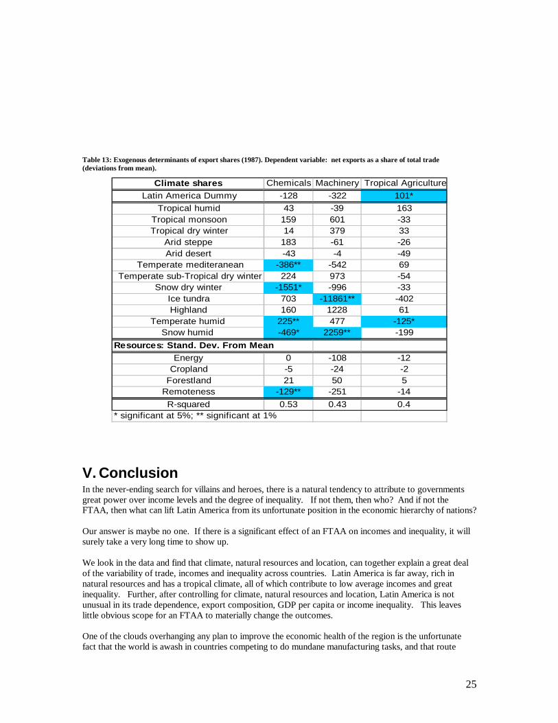
Table 13 shows how the countries’ exogenous characteristics affect the net exports shares in machinery,chemicals, and tropical agriculture, the three sectors empirically associated with income and inequalitymeasures. The reason to look at net exports shares instead of exports shares is that trade distortions may notpromote exports but instead lead to import substitution, what would be captured by the former but not bythe later variable. Once again the equations presented are weighted regressions with the variance of theresidual assumed to be equal to the labor force, thus producing regression estimates analogous to a meanwith weights equal to the labor force. There is no constant in the equation because the climate shares addto one. Furthermore, for computing the t-statistics, the mean has been subtracted from the dependentvariable, and the t-values on the climate proportions test if that climate zone is unusual compared with allthe others, not a test if the effect is zero. The resource variables are standardized to have mean zero andvariance one, thus allowing the coefficients on the climate variables to refer to the effect of climate on acountry with average endowments and to allow the coefficients on the resource variables to measure theeffect of a one-standard error increase. Finally a dummy variable for Latin American countries isintroduced to pick up disproportionate net export shares in those countries.

The results show that the trade patterns of the Latin American countries in chemicals, machinery, andtropical agriculture are not significantly distorted relatively to what would be predicted for countries withthe climates, locations, and resources in question. That leads us to conclude that the adoption of the FTAAagreement should not have a major impact on the regions’ export patterns and therefore should not affect,at least through this channel, the countries’ income and its distribution.

9 See the graphs available online at WWW where those countries are singled out.

25

Table 13: Exogenous determinants of export shares (1987). Dependent variable: net exports as a share of total trade(deviations from mean).

Climate shares Chemicals Machinery Tropical AgricultureLatin America Dummy -128 -322 101*

Tropical humid 43 -39 163Tropical monsoon 159 601 -33Tropical dry winter 14 379 33

Arid steppe 183 -61 -26Arid desert -43 -4 -49

Temperate mediteranean -386** -542 69Temperate sub-Tropical dry winter 224 973 -54

Snow dry winter -1551* -996 -33Ice tundra 703 -11861** -402Highland 160 1228 61

Temperate humid 225** 477 -125*Snow humid -469* 2259** -199

Resources: Stand. Dev. From MeanEnergy 0 -108 -12

Cropland -5 -24 -2Forestland 21 50 5

Remoteness -129** -251 -14R-squared 0.53 0.43 0.4

* significant at 5%; ** significant at 1%

V. ConclusionIn the never-ending search for villains and heroes, there is a natural tendency to attribute to governmentsgreat power over income levels and the degree of inequality. If not them, then who? And if not theFTAA, then what can lift Latin America from its unfortunate position in the economic hierarchy of nations?

Our answer is maybe no one. If there is a significant effect of an FTAA on incomes and inequality, it willsurely take a very long time to show up.

We look in the data and find that climate, natural resources and location, can together explain a great dealof the variability of trade, incomes and inequality across countries. Latin America is far away, rich innatural resources and has a tropical climate, all of which contribute to low average incomes and greatinequality. Further, after controlling for climate, natural resources and location, Latin America is notunusual in its trade dependence, export composition, GDP per capita or income inequality. This leaveslittle obvious scope for an FTAA to materially change the outcomes.

One of the clouds overhanging any plan to improve the economic health of the region is the unfortunatefact that the world is awash in countries competing to do mundane manufacturing tasks, and that route

26

toward progress is foreclosed by overcrowding. If there is a ray of hope, it comes from the examples ofCanada, Sweden and Finland, which are countries that are rich in natural resources but nonetheless havemanaged to attract high-wage complex manufacturing tasks. The successes of these countries surelydepend partly on education and closeness. From this is an essential lesson. The long-term economic healthof Latin America cannot be established without much improvement in education and without greatreductions of the economic, legal and cultural distance of the region from the high-income markets in NorthAmerica and Europe.

27

VI. References

• Acemoglu, Daron, Simon Johnson, and James A. Robinson. 2001. The Colonial Origins ofComparative Development: An Empirical Investigation, American Economic Review, 91(5):1369-1401.

• Acemoglu, Daron, Simon Johnson, and James A. Robinson. The Rise of Europe: Atlantic Trade,Instituional Change and Economic Growth, NBER working paper # 9378.

• Blum, Bernardo. S. 2001. Trade in Factor Services and Geography: An Account of Global Tradeand its Mysteries. UCLA mimeo.

• Deininger, Klaus and Lyn Squire. 1996. A New Data Set Measuring Income Inequality, The WorldBank Economic Review vol. 10(3): 565-91.

• Easterly, Willian, and Ross Levine. 2002. Tropics, Germs, and Crops: How EndowmentsInfluence Economic Development, NBER working paper # 9106.

• Engerman, Stanley L., and Kenneth L. Sokoloff, 1994. Factor Endowments, Institutions, andDifferential Paths of Growth Among New World Economies: A View from Economic Historians ofthe United States, NBER working paper # H0066.

• Feenstra, Robert C., R. E. Lipsey, and H. P. Bowen. 1997. World Trade Flows, 1970-1992, withproduction and tariff data, NBER working paper # 5910.

• Fujita, M., Paul Krugman, and Anthony Venables. 1999. The Spatial Economy: Cities, Regions,and International Trade, MIT Press, Cambridge MA.

• Hall, Robert, and Chad I Jones. 1999. Why do Some Countries Produce So Much more Output perWorker than Others?, Quarterly Journal of Economics 114(1): 83-116.

• Hillberry, R. and David Hummels. Explaining Home Bias in Consumption: the Role ofIntermediate Input Trade, NBER working paper # 9020.

• Leamer, Edward E. 1984. Sources of international comparative advantage: theory and evidence,The MIT Press.

• Leamer, Edward. E. 1987. Paths of Development in the Three-Factor, n-Good GeneralEquilibrium Model, Journal of Political Economy, Vol. 95 (5): 961-999.

• Leamer, Edward E. 1999. Effort, Wages and the International Division of Labor, Journal ofPolitical Economy, Vol. 107(6): 1127-1163. Reprinted in Singer, Hans et.al. New World OrderSeries, Vol. 20, 2001.

• Leamer, Edward E. and Christopher Thornberg. 2000. Effort and Wages: A New Look at the Inter-Industry Wage Differentials. In The Impact of International Trade on Wages, edited by RobertFeenstra. NBER: The University of Chicago Press, 2000: 37-84.

• Leamer, Edward E. 1997. Access to Western Markets and Eastern Effort. In Lessons from theEconomic Transition, Central and Eastern Europe in the 1990s, edited Salvatore Zecchini.Dordrecht: Kluwer Academic Publishers: pp. 503-526.

• Leamer, Edward E., Hugo Maul, Sergio Rodriquez and Peter Schott. 1999. Does natural resourceabundance increase Latin American income inequality?, Journal of Development Economics, Vol.59(1): pp. 3-42.

• Leamer, Edward E. and Michael Storper. 2001. The Economic Geography of the Internet Age,Journal of International Business Studies, 32(4): 641-655.

• Machiavelli, N. 1519. Discourses on Livy, (Oxford University Press, New York, 1987).• Overman, Henry G., Stephen Redding and Anthony J. Venables. 2001. The Economic Geography

of Trade, Production, Nad Income: A Survey of Empirics, mimeo.• Redding, Stephen, and Peter K. Schott. 2002. Distance, Skill Deepening and Development: Will

Peripheral Countries Ever Get Rich?, mimeo.• Rodrik, D., A. Subramanian and F. Trebbi. 2002. Institutions rule: the primacy of institutions over

geography and integration in economic development, NBER working paper # 9305.• Sachs, Jeffrey D. and John W. McArthur. 2001. Institutions and Geography: Comment on

Acemoglu, Johnson, and Robinson (2000), NBER working paper # 8814.• Sachs, J. D. 2001. Tropical underdevelopment, NBER working paper # 8119.

28

• Strauss-Kahn, Vanessa. 2001. Globalization, Agglomeration, and Wage Premia, mimeo.• Venables, Anthony. and Nuno Limao. 2002. Geographical Disadvantage: A Heckscher-Ohlin-Von

Thunen Model of International Specialization, Journal of International Economics, 58(2).