Embed Size (px)
Citation preview
MEDICAL IMAGE
REGISTRATION
AND
SURGERY SIMULATION
IMM-PHD-1996-25
Morten Bro-Nielsen
July 26, 1997

ii
Preface
This thesis has been prepared at the Department of Mathematical Modelling(IMM), Technical University of Denmark. It is a partial fulllment of the re-quirements for the degree of Ph.D. in engineering.
The subject is Medical Image Registration and Surgery Simulation, with aspecic focus on the physical models used in these elds.
Many of the techniques, described and developed in the thesis, are on theforefront of technology and, therefore, do not always have practical applicationstoday. But, I hope the reader will read the thesis with an open mind, andenjoy the perspectives which some of the techniques open up for the future oftechnology in medicine.
Reading this thesis requires a basic knowledge of image analysis, computergraphics, physical models, and the nomenclature used in medical image analysis.
Lyngby, August 1996
Morten Bro-Nielsen
iii

iv PREFACE
Acknowledgements
The work reported in this thesis has been carried out at three dierent locations:The Department of Mathematical Modelling (IMM) at the Technical Universityof Denmark, the Epidaure group at INRIA, France, and the 3D-Lab at theSchool of Dentistry, University of Copenhagen, Denmark.
It was during the 9 months I spent in the Epidaure group, that the mainbasis and ideas of this thesis were developed. I would, therefore, like to thankdr. Nicholas Ayache, very much, for giving me the chance to work there. It wasa source of continuous inspiration and great fun to interact with the membersof the group, and I am grateful to everybody there. In particular, I wouldlike to thank dr. Herve Delingette who never tired of answering my questionson Euler-Lagrange equations, and Stephane Cotin with whom I shared manyfruitful discussions on surgery simulation.
After I returned to Denmark, I have spent most of my time at the 3D-Lab inCopenhagen. The 3D-Lab is a joint research center for the National UniversityHospital of Denmark, the School of Dentistry, University of Copenhagen, andIMM at the Technical University of Denmark.
Professor Sven Kreiborg of the School of Dentistry has been the driving forcebehind the 3D-Lab. I would like to thank Sven for allowing me to work there,and for the many insights into medicine and dentistry, which he has given me.In addition, I am grateful to Per Larsen and especially Tron Darvann for theirtremendous help with practical issues.
During the Ph.D., I have been the supervisor for four M.Sc. thesis students.Working with these students has been a source of inspiration for much of thework, which is in this thesis. I would, therefore, like to thank Rolf Jackson,Michael Konstantinidis, Bo Rasmussen, and especially Claus Gramkow, for theeort, and energy they put into their work - and also the fun we had together.
Dr. Mads Nielsen from the department of Computer Science, the Universityof Copenhagen, has also been a great inspiration throughout the project. Hisexplanations of theoretical aspects of scale-space and regularization, both orallyand in papers, have been important for my basic understanding of physicalmodels.
I would like to thank my supervisors, professor Knut Conradsen and dr.Bjarne Kjr Ersbll, and the rest of the Image Analysis Group at IMM for thechance to work on this Ph.D. thesis. In particular, I would like to thank Knutfor always backing me up, whenever I got into trouble. Also the TAP people
v
vi ACKNOWLEDGEMENTS
at IMM, especially Helle Welling, Finn Kuno Christensen, Else Johansen, andRuth Bredsdor, deserve credit for their loyal support and help with all thepractical things.
My sister Helle Bro-Nielsen helped tremendously during the last hectic week,with proof-reading and correction of the manuscript. Many thanks to her also.
This thesis was mainly supported by the Technical University of Denmark,and partly by the Danish Research Academy and Knud Hjgards Foundation.
For typesetting the LATEX2" package has been used.
This thesis is dedicated to KMB.
Summary
This thesis explores the application of physical models in medical image regis-tration and surgery simulation. The continuum models of elasticity and viscous uids are described in detail, and this knowledge is used as a basis for most ofthe methods described here.
Rigid image registration using voxel similarity measures are reviewed, andnew measures based on Grey Level Cooccurrence Matrices (GLCM) are intro-duced. These measures are evaluated extensively using CT, MR, and cryosectionimages from the Visible Human data set. The results show that mutual infor-mation remains the best generally applicable measure. But for specic modalitycombinations the new GLCM measures show considerable promise.
Results of registering the CT image to the red channel of the cryosectionimage, and the CT image to the MR image are shown.
A new and faster algorithm for non-rigid registration using viscous uidmodels is presented. This algorithm replaces the core part of the original al-gorithm with multi-resolution convolution using a new lter, which implementsthe linear elasticity operator. Using the lter results in a speedup of at leastan order of magnitude. Use of convolution hardware is expected to improve theperformance even more.
Non-rigid registration using a physically valid model of bone growth is alsopresented. Using medical knowledge about the growth processes of the mandibu-lar bone, a registration algorithm for time sequence images of the mandible isdeveloped. Since this registration algorithm models the actual development ofthe mandible, it is possible to simulate the development.
Finally, real-time deformable models, using nite element models of linearelasticity, are developed for surgery simulation. The time consumption of thenite element method is reduced dramaticly, by the use of condensation tech-niques, explicit inversion of the stiness matrix, and the use of selective matrixvector multiplication.
Reviews of both medical image registration and surgery simulation work aregiven.
Keywords: Medical image registration, rigid registration, non-rigid registra-tion, grey level cooccurrence matrices, Visible Human data set, voxel sim-ilarity measures, physical models, continuum models, elastic models, vis-cous uid models, linear elasticity, convolution, elastic registration, uid
vii

viii SUMMARY
registration, bone growth, growth models, virtual reality, surgery simula-tion, cranio-facial surgery simulation, nite element models, condensation,linear matrix systems.
Resume
Denne afhandling behandler anvendelsen af fysiske modeller i medicinsk bille-dregistrering og operationssimulering. Kontinuummodeller for elasticitet ogviskose uider beskrives detaljeret, og viden om disse modeller danner basisfor de este af de metoder der beskrives i afhandlingen.
Rigid billedregistrering vha. voxel-similaritetsmal beskrives, og nye mal baseretpa Grey Level Cooccurrence Matrices (GLCM) introduceres. Disse mal testesvha. CT, MT, og histologiske snitbilleder fra Visible Human databasen. Re-sultaterne viser at mutual information forbliver det bedste generelt anvendeligemal til rigid registrering. Men, for enkelte modalitetskombinationer viser de nyeGLCM mal lovende muligheder.
Resultater vises for registrering af CT billede til den rde kanal af det his-tologiske snitbillede, og CT billede til MR billede.
En ny og hurtigere algoritme til ikke-rigid registrering vha. viskose uidemodeller prsenteres. Denne algoritme erstatter den centrale del af den originalealgoritme, med multi-skala konvolution vha. et nyt lter, som implementererden linert elastiske operator. Ved at anvende dette lter opnas en hastigheds-forgelse pa mindst en faktor. Med specialiseret konvolutions-hardware kanendnu hurtigere behandling forventes.
Ikke-rigid registrering vha. en fysisk korrekt model af knoglevkst beskri-ves ogsa. Med medicinsk viden om vkstprocesserne i mandiblen, udvikles enregistreringsalgoritme til registrering af tidssekvensbilleder af mandiblen. Sidenregistreringsalgoritmen modellerer den egentlige udvikling af mandiblen, er detmuligt at simulere denne udvikling.
Endelig udvikles real-tids deformerbare modeller til operationssimuleringvha. nite element modeller af liner elasticitet. Disse modellers tidsforbrugreduceres kraftigt vha. kondenseringsteknikker, eksplicit invertering af stivheds-matricen, og anvendelsen af selektiv matrix vektor multiplicering.
Reviews af bade medicinsk billedregistrering og operationssimulering gives.
Ngleord: Medicinsk billedregistrering, rigid registrering, ikke-rigid registrering,grey level cooccurrence matrices, Visible Human databasen, voxel-similaritetsmal,fysiske modeller, kontinuummodeller, elastiske modeller, viskose uidemodeller, liner elasticitet, konvolution, elastisk registrering, uid reg-istrering, knoglevkst, vkstmodeller, virtual reality, operationssimuler-ing, cranio-facial operationssimulering, nite element modeller, kondenser-
ix

x RESUME
ing, linere matrixsystemer.
Publications During Ph.D.
This section lists the publications and other work, which have been producedduring the Ph.D. period.
Int. Publications related to this thesis
[BN96e] M. Bro-Nielsen and C. Gramkow, Fast uid registration of medicalimages, accepted for Visualization in Biomedical Computing (VBC'96),1996
[BN96d] M. Bro-Nielsen, Surgery simulation using fast nite elements,poster, accepted for Visualization in Biomedical Computing (VBC'96),1996
[BN96c] M. Bro-Nielsen and S. Cotin, Real-time volumetric deformablemodels for surgery simulation using nite elements and condensation,Computer Graphics Forum, 15(3):57-66 (Eurographics'96), 1996
[BN96] M. Bro-Nielsen, Mvox: Interactive 2-4D medical image and graph-ics visualization software, proc. Computer Assisted Radiology (CAR'96),pp. 335-338, 1996
[Cot96] S. Cotin, H. Delingette, M. Bro-Nielsen, N. Ayache, J.M. Clement,V. Tassetti and J. Marescaux, Geometric and Physical representations fora simulator of hepatic surgery, proc. Medicine Meets Virtual Reality, 1996
[BN95b] M. Bro-Nielsen and S. Cotin, Soft tissue modelling in surgery sim-ulation for prediction of results of craniofacial operations & steps towardsvirtual reality training systems, abstract, proc. 3rd Int.Workshop on Rapid Prototyping in Medicine & Computer-Assisted Sur-gery, 1995
[BN95] M. Bro-Nielsen, Modelling elasticity in solids using Active Cubes- Application to simulated operations, proc. Computer Vision, VirtualReality and Robotics in Medicine (CVRMed'95), pp. 535-541, 1995
xi
xii PUBLICATIONS DURING PH.D.
Int. Publications not related to this thesis
L. Bjoerndal, T. Darvann, M. Bro-Nielsen and A. Thylstrup, Automatedimage analysis applied on odontoblast reactions to caries, abstract, ac-cepted for Journal of Caries Research, 1996
T. Darvann, M. Bro-Nielsen, K. Damgaard, U. Knigge, P. Larsen, and L.B.Svendsen, A possible concept for an interactive 3D visualization system fortraining and planning of liver surgery, proc. Medical Informatics Europe(MIE'96), pp. 1052-1054, 1996
M. Bro-Nielsen, P. Larsen and S. Kreiborg, Virtual teeth: A 3D methodfor editing and visualizing small structures in CT scans, proc. ComputerAssisted Radiology (CAR'96), pp. 921-924, 1996
S. Kreiborg, P. Larsen, M. Bro-Nielsen and T. Darvann, A 3-dimensio-nal analysis of tooth formation and eruption in a case of Apert syndrome,poster, proc. Computer Assisted Radiology (CAR'96), pp. 1066-1068,1996
B. Nikkhade-Dehkordi, M. Bro-Nielsen, T. Darvann, C. Gramkow, N.Egund and K. Hermann, 3D reconstruction of the femoral bone using twoX-ray images from orthogonal views, poster, proc. Computer AssistedRadiology (CAR'96), pp. 1015, 1996
M. Bro-Nielsen, K. Suzuki and M. Watanabe, 3D Modeling Method fromOccluding Contours by Geometric Primitives, proc. Asian Conf. Com-puter Vision (ACCV'93), pp. 221-225, 1993
K. Suzuki, T. Wada and M. Bro-Nielsen, Automatic Object Modelingbased on Multiview Sensing Images, proc. Asian Conf. Computer Vision(ACCV'93), pp. 244-247, 1993
Technical reports
M. Bro-Nielsen, 3D models from occluding contours using geometric prim-itives, IMM Tech. Rep. 94-15, 1994
M. Bro-Nielsen, Modelling elasticity in solids using active cubes - applica-tion to simulated operations, IMM Tech. Rep. 94-14, 1994
M. Bro-Nielsen, Active Nets and Cubes, IMM Tech. Rep. 94-13, 1994
M. Bro-Nielsen, Parallel implementation of Active Nets, IMM Tech. Rep.,1994
xiii
Supervised M.Sc. theses
[Ras96] Bo Rasmussen, Craniofacial surgery simulation, 1996
Michael Konstantinidis, Registration and segmentation of medical images,1996
[Gra96] Claus Gramkow, Registration of 2D and 3D medical images, 1996
Rolf Jackson, On the analysis of 3D images, 1995
Mvox software package
A software package for visualization and segmentation of medical images hasbeen developed during the Ph.D. [BN96, BN96b]. The software, which is calledMvox, has been commercialized and is being sold by the company Mware. Itwas displayed at the Computer Assisted Radiology (CAR'96) symposium 1996,where it received a very positive response. Appendix A gives a brief intro-duction to Mvox. For additional information, please refer to the Mvox WWWhomepage [BN96b].

xiv PUBLICATIONS DURING PH.D.

Contents
Preface iii
Acknowledgements v
Summary vii
Resume ix
Publications During Ph.D. xi
List of Figures xviii
List of Tables xxii
1 Introduction 11.1 Physical models . . . . . . . . . . . . . . . . . . . . . . . . . . . . 21.2 Medical workstation of the future . . . . . . . . . . . . . . . . . . 31.3 Thesis overview . . . . . . . . . . . . . . . . . . . . . . . . . . . . 31.4 Thesis contributions . . . . . . . . . . . . . . . . . . . . . . . . . 41.5 Credit . . . . . . . . . . . . . . . . . . . . . . . . . . . . . . . . . 5
1.5.1 Viscous uid registration . . . . . . . . . . . . . . . . . . 61.5.2 Fast Finite Elements . . . . . . . . . . . . . . . . . . . . . 61.5.3 Growth registration . . . . . . . . . . . . . . . . . . . . . 6
2 Medical Image Registration 72.1 Motion model . . . . . . . . . . . . . . . . . . . . . . . . . . . . . 9
2.1.1 Rigid motion . . . . . . . . . . . . . . . . . . . . . . . . . 92.1.2 Elastic motion . . . . . . . . . . . . . . . . . . . . . . . . 92.1.3 Free motion . . . . . . . . . . . . . . . . . . . . . . . . . . 102.1.4 Parameter space . . . . . . . . . . . . . . . . . . . . . . . 10
2.2 Driving potential/force . . . . . . . . . . . . . . . . . . . . . . . . 102.2.1 Point methods . . . . . . . . . . . . . . . . . . . . . . . . 112.2.2 Curve methods . . . . . . . . . . . . . . . . . . . . . . . . 112.2.3 Surface methods . . . . . . . . . . . . . . . . . . . . . . . 122.2.4 Moments and principal axes methods . . . . . . . . . . . 13
xv
xvi CONTENTS
2.2.5 Voxel similarity methods . . . . . . . . . . . . . . . . . . . 132.3 Registration to electronic atlases . . . . . . . . . . . . . . . . . . 142.4 Summary . . . . . . . . . . . . . . . . . . . . . . . . . . . . . . . 15
3 Rigid Registration using Voxel Similarity Measures 173.1 Image data . . . . . . . . . . . . . . . . . . . . . . . . . . . . . . 173.2 Voxel similarity measures . . . . . . . . . . . . . . . . . . . . . . 19
3.2.1 GLCM matrices . . . . . . . . . . . . . . . . . . . . . . . 203.2.2 GLCM features . . . . . . . . . . . . . . . . . . . . . . . . 253.2.3 Implementation . . . . . . . . . . . . . . . . . . . . . . . . 293.2.4 Plotting GLCM features . . . . . . . . . . . . . . . . . . . 313.2.5 Results . . . . . . . . . . . . . . . . . . . . . . . . . . . . 323.2.6 Adaptive position-dependent weights . . . . . . . . . . . . 33
3.3 Image registration using voxel similarity measures . . . . . . . . 353.4 Summary . . . . . . . . . . . . . . . . . . . . . . . . . . . . . . . 35
4 Physical Continuum Models 434.1 Introduction . . . . . . . . . . . . . . . . . . . . . . . . . . . . . . 434.2 Mathematical preliminaries . . . . . . . . . . . . . . . . . . . . . 454.3 Continuum models . . . . . . . . . . . . . . . . . . . . . . . . . . 46
4.3.1 Denitions . . . . . . . . . . . . . . . . . . . . . . . . . . 474.3.2 Strain . . . . . . . . . . . . . . . . . . . . . . . . . . . . . 494.3.3 Forces . . . . . . . . . . . . . . . . . . . . . . . . . . . . . 504.3.4 Equations of motion for a continuum . . . . . . . . . . . . 51
4.4 Elastic continuum models . . . . . . . . . . . . . . . . . . . . . . 534.4.1 Mooney-Rivlin materials . . . . . . . . . . . . . . . . . . . 554.4.2 St. Venant Kirchho materials . . . . . . . . . . . . . . . 554.4.3 Linear elastic materials . . . . . . . . . . . . . . . . . . . 55
4.5 Viscous uid continuum models . . . . . . . . . . . . . . . . . . . 574.6 Eigen-function parametrization of the linear elastic operator . . . 58
4.6.1 Projection of forces onto the eigen-function basis . . . . . 614.6.2 2D eigen-function basis . . . . . . . . . . . . . . . . . . . 61
4.7 Summary . . . . . . . . . . . . . . . . . . . . . . . . . . . . . . . 62
5 Non-rigid Registration using Continuum Models 635.1 Dening the problem . . . . . . . . . . . . . . . . . . . . . . . . . 645.2 Elastic registration . . . . . . . . . . . . . . . . . . . . . . . . . . 645.3 Viscous uid registration . . . . . . . . . . . . . . . . . . . . . . . 67
5.3.1 Viscous uid model . . . . . . . . . . . . . . . . . . . . . 675.3.2 Force eld . . . . . . . . . . . . . . . . . . . . . . . . . . . 685.3.3 Numerical solution . . . . . . . . . . . . . . . . . . . . . . 695.3.4 Solving the linear PDE . . . . . . . . . . . . . . . . . . . 705.3.5 Convolution lter for linear elasticity . . . . . . . . . . . . 715.3.6 Multi-resolution implementation . . . . . . . . . . . . . . 755.3.7 Results . . . . . . . . . . . . . . . . . . . . . . . . . . . . 75
5.4 Comparing uid with 'demon'-based registration . . . . . . . . . 82

CONTENTS xvii
5.4.1 Characteristics of the Gaussian lter . . . . . . . . . . . . 825.4.2 The Gaussian versus linear elastic lter for registration . 84
5.5 Timings . . . . . . . . . . . . . . . . . . . . . . . . . . . . . . . . 845.6 Summary . . . . . . . . . . . . . . . . . . . . . . . . . . . . . . . 88
6 Non-Rigid Registration using Bone Growth Model 896.1 Non-rigid registration as a physical problem . . . . . . . . . . . . 906.2 Bone growth . . . . . . . . . . . . . . . . . . . . . . . . . . . . . 92
6.2.1 Growth of the mandible . . . . . . . . . . . . . . . . . . . 926.2.2 Stable structures . . . . . . . . . . . . . . . . . . . . . . . 93
6.3 Non-rigid registration of mandibles using bone growth model . . 936.3.1 Rigid registration of stable structures . . . . . . . . . . . 946.3.2 Growth model . . . . . . . . . . . . . . . . . . . . . . . . 946.3.3 Implementation . . . . . . . . . . . . . . . . . . . . . . . . 976.3.4 Results . . . . . . . . . . . . . . . . . . . . . . . . . . . . 98
6.4 Summary . . . . . . . . . . . . . . . . . . . . . . . . . . . . . . . 99
7 Soft Tissue Modeling in Surgery Simulation 1017.1 Cranio-facial surgery simulation . . . . . . . . . . . . . . . . . . . 1017.2 Minimally invasive surgery simulation . . . . . . . . . . . . . . . 1027.3 Technical requirements . . . . . . . . . . . . . . . . . . . . . . . . 1027.4 Previous work . . . . . . . . . . . . . . . . . . . . . . . . . . . . . 104
7.4.1 Cranio-facial surgery simulation models . . . . . . . . . . 1057.4.2 Real-time surgery simulation models . . . . . . . . . . . . 1087.4.3 Work for the future . . . . . . . . . . . . . . . . . . . . . 108
7.5 Summary . . . . . . . . . . . . . . . . . . . . . . . . . . . . . . . 109
8 Real-time Deformable Models for Surgery Simulation 1118.1 Choice of model . . . . . . . . . . . . . . . . . . . . . . . . . . . . 1128.2 Linear elastic material model . . . . . . . . . . . . . . . . . . . . 1138.3 Discretization using FE model . . . . . . . . . . . . . . . . . . . . 114
8.3.1 Fixing nodes . . . . . . . . . . . . . . . . . . . . . . . . . 1178.4 Simplifying the system using condensation . . . . . . . . . . . . . 1178.5 Solving the linear matrix system . . . . . . . . . . . . . . . . . . 1188.6 Simulation . . . . . . . . . . . . . . . . . . . . . . . . . . . . . . . 119
8.6.1 Dynamic system . . . . . . . . . . . . . . . . . . . . . . . 1198.6.2 Static system and selective matrix vector multiplication . 1218.6.3 Summary of simulation methods . . . . . . . . . . . . . . 122
8.7 Simulation system . . . . . . . . . . . . . . . . . . . . . . . . . . 1228.7.1 Mesh generation using Mvox and Nuages . . . . . . . . . 1228.7.2 SGI Performer parallel pipe-lining system . . . . . . . . . 123
8.8 Results . . . . . . . . . . . . . . . . . . . . . . . . . . . . . . . . . 1278.9 Extensions . . . . . . . . . . . . . . . . . . . . . . . . . . . . . . . 130
8.9.1 Domain decomposition . . . . . . . . . . . . . . . . . . . . 1308.9.2 Cutting in nite element systems . . . . . . . . . . . . . . 132
8.10 Summary . . . . . . . . . . . . . . . . . . . . . . . . . . . . . . . 133
xviii CONTENTS
9 Conclusion 137
A Mvox 139
B Derivation of Linear Filter. 145
C Linear Tetrahedral Finite Element 147
D GLCM Plots 149D.1 MR-Pd / MR-T1 (moved) . . . . . . . . . . . . . . . . . . . . . . 149D.2 CT Bone / MR-T1 (moved) . . . . . . . . . . . . . . . . . . . . . 170D.3 CT Bone (moved) / Red . . . . . . . . . . . . . . . . . . . . . . . 191
Bibliography 213
Index 228
Ph.D. theses from IMM 228
List of Figures
1.1 Dual view of medical image registration and surgery simulation. . 2
2.1 Rigid, elastic, and free motion. . . . . . . . . . . . . . . . . . . . 9
3.1 Images from the Visible Human data set . . . . . . . . . . . . . . 183.2 GLCM matrix for T1/T1 . . . . . . . . . . . . . . . . . . . . . . 213.3 GLCM matrix for PD/T1 . . . . . . . . . . . . . . . . . . . . . . 223.4 GLCM matrix for CT/T1 . . . . . . . . . . . . . . . . . . . . . . 233.5 GLCM matrix for CT/R . . . . . . . . . . . . . . . . . . . . . . . 243.6 Weighting functions for energy and entropy. . . . . . . . . . . . . 283.7 Weights for the position dependent GLCM features . . . . . . . . 293.8 CT/T1 result of registration using mutual information . . . . . . 363.9 CT/T1 result of registration using mutual information . . . . . . 373.10 CT/T1 result of registration using mutual information . . . . . . 383.11 CT/R result of registration using mutual information . . . . . . . 393.12 CT/R result of registration using mutual information . . . . . . . 403.13 CT/R result of registration using mutual information . . . . . . . 41
4.1 Relationship between physical entities. . . . . . . . . . . . . . . . 444.2 Deformation of the body . . . . . . . . . . . . . . . . . . . . . . 464.3 Denition of displacement. . . . . . . . . . . . . . . . . . . . . . . 47
5.1 Registering a 2D square to a rectangle using linear elastic regis-tration . . . . . . . . . . . . . . . . . . . . . . . . . . . . . . . . . 65
5.2 Registering a 2D square to a rectangle using viscous uid regis-tration . . . . . . . . . . . . . . . . . . . . . . . . . . . . . . . . . 66
5.3 Displacements of 2D linear elastic lter. . . . . . . . . . . . . . . 745.4 Comparison of FEM and lter solution for complex deformation 765.5 Circle to 'C' using viscous uid registration . . . . . . . . . . . . 775.6 Deformation of grid for circle to 'C' using viscous uid registration 785.7 CT slice registered to another slice using viscous uid model . . 795.8 MR slice registered to another slice using viscous uid model . . 805.9 Fluid registration of 3 binary jaw images . . . . . . . . . . . . . . 815.10 Comparison between the linear elastic and Gaussian lters for
the patch to 'C' experiment . . . . . . . . . . . . . . . . . . . . . 85
xix
xx LIST OF FIGURES
5.11 Comparison between the linear elastic and Gaussian lters forthe circle to 'C' experiment . . . . . . . . . . . . . . . . . . . . . 86
5.12 Comparison between the linear elastic and Gaussian lters forthe square to rectangle experiment . . . . . . . . . . . . . . . . . 87
6.1 Dierent registration methods. . . . . . . . . . . . . . . . . . . . 916.2 Images of the mandible of a child. . . . . . . . . . . . . . . . . . 916.3 Anatomic description of the mandible. . . . . . . . . . . . . . . . 926.4 Stable features in the mandible. . . . . . . . . . . . . . . . . . . . 936.5 Overlayed mandibles after rigid registration. . . . . . . . . . . . . 946.6 Domain denitions . . . . . . . . . . . . . . . . . . . . . . . . . . 956.7 Growth speed considerations . . . . . . . . . . . . . . . . . . . . 966.8 Line process. . . . . . . . . . . . . . . . . . . . . . . . . . . . . . 976.9 2D growth template images . . . . . . . . . . . . . . . . . . . . . 986.10 2D growth using simple velocity . . . . . . . . . . . . . . . . . . . 986.11 2D growth using distance dependent velocity . . . . . . . . . . . 996.12 Result of growth registration of 3 binary jaw images. . . . . . . . 100
7.1 Soft tissue models for realistic and real-time simulation . . . . . 1057.2 Active cube is deformed to match the shape of a patient. . . . . 1067.3 Modeling soft tissue change using active cube . . . . . . . . . . . 107
8.1 Solid elastic object. . . . . . . . . . . . . . . . . . . . . . . . . . . 1138.2 Discretization of domain into tetrahedral elements . . . . . . . . 1158.3 Voxel data from the visible human data set. . . . . . . . . . . . . 1238.4 Contours created using Mvox . . . . . . . . . . . . . . . . . . . . 1248.5 FE mesh created from contours using Nuages . . . . . . . . . . . 1258.6 Simulation system implemented using SGI Performer. . . . . . . 1268.7 Simulation system diagram . . . . . . . . . . . . . . . . . . . . . 1268.8 Wireframe model of lower leg in simulator. . . . . . . . . . . . . 1278.9 Simulation of pushing on a the lower leg . . . . . . . . . . . . . . 1288.10 Simulation of pulling on a the lower leg . . . . . . . . . . . . . . 1298.11 Domain decomposition. . . . . . . . . . . . . . . . . . . . . . . . 1318.12 Simple cutting in nite element mesh. . . . . . . . . . . . . . . . 134
A.1 Mvox main 2D image handling window. . . . . . . . . . . . . . . 140A.2 Mvox thresholding window. . . . . . . . . . . . . . . . . . . . . . 141A.3 Mvox drawing window. . . . . . . . . . . . . . . . . . . . . . . . . 142A.4 Mvox 3D graphics window. . . . . . . . . . . . . . . . . . . . . . 143A.5 Mvox 3D volume rendering window. . . . . . . . . . . . . . . . . 144
D.1 Pd/T1: Distance/energy . . . . . . . . . . . . . . . . . . . . . . . 152D.2 Pd/T1: Distance/variance . . . . . . . . . . . . . . . . . . . . . . 153D.3 Pd/T1: Distance/entropy . . . . . . . . . . . . . . . . . . . . . . 154D.4 Pd/T1: Distance/MI . . . . . . . . . . . . . . . . . . . . . . . . . 155D.5 Pd/T1: Distance/IDM . . . . . . . . . . . . . . . . . . . . . . . . 156

LIST OF FIGURES xxi
D.6 Pd/T1: Distance/inertia . . . . . . . . . . . . . . . . . . . . . . . 157D.7 Pd/T1: Distance/Dmoment . . . . . . . . . . . . . . . . . . . . . 158D.8 Pd/T1: Distance/correlation . . . . . . . . . . . . . . . . . . . . 159D.9 Pd/T1: Distance/Cshade . . . . . . . . . . . . . . . . . . . . . . 160D.10 Pd/T1: Distance/Cprominence . . . . . . . . . . . . . . . . . . . 161D.11 Pd/T1: Distance/Woods MR/PET X-xed . . . . . . . . . . . . 162D.12 Pd/T1: Distance/Woods MR/PET X-moved . . . . . . . . . . . 163D.13 Pd/T1: Sequence plots of energy. . . . . . . . . . . . . . . . . . . 164D.14 Pd/T1: Sequence plots of variance. . . . . . . . . . . . . . . . . . 164D.15 Pd/T1: Sequence plots of entropy. . . . . . . . . . . . . . . . . . 165D.16 Pd/T1: Sequence plots of MI. . . . . . . . . . . . . . . . . . . . . 165D.17 Pd/T1: Sequence plots of IDM. . . . . . . . . . . . . . . . . . . . 166D.18 Pd/T1: Sequence plots of inertia. . . . . . . . . . . . . . . . . . . 166D.19 Pd/T1: Sequence plots of Dmoment. . . . . . . . . . . . . . . . . 167D.20 Pd/T1: Sequence plots of correlation. . . . . . . . . . . . . . . . 167D.21 Pd/T1: Sequence plots of Cshade. . . . . . . . . . . . . . . . . . 168D.22 Pd/T1: Sequence plots of Cprominence. . . . . . . . . . . . . . . 168D.23 Pd/T1: Sequence plots of woods MR/PET X-xed. . . . . . . . . 169D.24 Pd/T1: Sequence plots of woods MR/PET X-moved. . . . . . . . 169D.25 CT/T1: Distance/energy . . . . . . . . . . . . . . . . . . . . . . 173D.26 CT/T1: Distance/variance . . . . . . . . . . . . . . . . . . . . . . 174D.27 CT/T1: Distance/entropy . . . . . . . . . . . . . . . . . . . . . . 175D.28 CT/T1: Distance/MI . . . . . . . . . . . . . . . . . . . . . . . . 176D.29 CT/T1: Distance/IDM . . . . . . . . . . . . . . . . . . . . . . . 177D.30 CT/T1: Distance/inertia . . . . . . . . . . . . . . . . . . . . . . 178D.31 CT/T1: Distance/Dmoment . . . . . . . . . . . . . . . . . . . . . 179D.32 CT/T1: Distance/correlation . . . . . . . . . . . . . . . . . . . . 180D.33 CT/T1: Distance/Cshade . . . . . . . . . . . . . . . . . . . . . . 181D.34 CT/T1: Distance/Cprominence . . . . . . . . . . . . . . . . . . . 182D.35 CT/T1: Distance/Woods MR/PET X-xed . . . . . . . . . . . . 183D.36 CT/T1: Distance/Woods MR/PET X-moved . . . . . . . . . . . 184D.37 CT/T1: Sequence plots of energy. . . . . . . . . . . . . . . . . . . 185D.38 CT/T1: Sequence plots of variance. . . . . . . . . . . . . . . . . 185D.39 CT/T1: Sequence plots of entropy. . . . . . . . . . . . . . . . . . 186D.40 CT/T1: Sequence plots of MI. . . . . . . . . . . . . . . . . . . . 186D.41 CT/T1: Sequence plots of IDM. . . . . . . . . . . . . . . . . . . 187D.42 CT/T1: Sequence plots of inertia. . . . . . . . . . . . . . . . . . 187D.43 CT/T1: Sequence plots of Dmoment. . . . . . . . . . . . . . . . . 188D.44 CT/T1: Sequence plots of correlation. . . . . . . . . . . . . . . . 188D.45 CT/T1: Sequence plots of Cshade. . . . . . . . . . . . . . . . . . 189D.46 CT/T1: Sequence plots of Cprominence. . . . . . . . . . . . . . . 189D.47 CT/T1: Sequence plots of woods MR/PET X-xed. . . . . . . . 190D.48 CT/T1: Sequence plots of woods MR/PET X-moved. . . . . . . 190D.49 CT/R: Distance/energy . . . . . . . . . . . . . . . . . . . . . . . 194D.50 CT/R: Distance/variance: Rotation only, Translation only, Nor-
mal and Corrected. . . . . . . . . . . . . . . . . . . . . . . . . . . 195
xxii LIST OF FIGURES
D.51 CT/R: Distance/entropy . . . . . . . . . . . . . . . . . . . . . . . 196D.52 CT/R: Distance/MI . . . . . . . . . . . . . . . . . . . . . . . . . 197D.53 CT/R: Distance/IDM . . . . . . . . . . . . . . . . . . . . . . . . 198D.54 CT/R: Distance/inertia . . . . . . . . . . . . . . . . . . . . . . . 199D.55 CT/R: Distance/Dmoment . . . . . . . . . . . . . . . . . . . . . 200D.56 CT/R: Distance/correlation . . . . . . . . . . . . . . . . . . . . . 201D.57 CT/R: Distance/Cshade . . . . . . . . . . . . . . . . . . . . . . . 202D.58 CT/R: Distance/Cprominence . . . . . . . . . . . . . . . . . . . . 203D.59 CT/R: Distance/Woods MR/PET X-xed . . . . . . . . . . . . . 204D.60 CT/R: Distance/Woods MR/PET X-moved . . . . . . . . . . . . 205D.61 CT/R: Sequence plots of energy. . . . . . . . . . . . . . . . . . . 206D.62 CT/R: Sequence plots of variance. . . . . . . . . . . . . . . . . . 206D.63 CT/R: Sequence plots of entropy. . . . . . . . . . . . . . . . . . . 207D.64 CT/R: Sequence plots of MI. . . . . . . . . . . . . . . . . . . . . 207D.65 CT/R: Sequence plots of IDM. . . . . . . . . . . . . . . . . . . . 208D.66 CT/R: Sequence plots of inertia. . . . . . . . . . . . . . . . . . . 208D.67 CT/R: Sequence plots of Dmoment. . . . . . . . . . . . . . . . . 209D.68 CT/R: Sequence plots of correlation. . . . . . . . . . . . . . . . . 209D.69 CT/R: Sequence plots of Cshade. . . . . . . . . . . . . . . . . . . 210D.70 CT/R: Sequence plots of Cprominence. . . . . . . . . . . . . . . . 210D.71 CT/R: Sequence plots of woods MR/PET X-xed. . . . . . . . . 211D.72 CT/R: Sequence plots of woods MR/PET X-moved. . . . . . . . 211
List of Tables
3.1 Pd-T1: Similarity measure plot . . . . . . . . . . . . . . . . . . . 333.2 CT/T1: Similarity measure plot . . . . . . . . . . . . . . . . . . 343.3 CT/R: Similarity measure plot . . . . . . . . . . . . . . . . . . . 34
5.1 Timings for 2D viscous uid registration experiments . . . . . . . 88
D.1 Pd/T1: Regression results . . . . . . . . . . . . . . . . . . . . . . 150D.2 Pd/T1: Corrected linear regression results . . . . . . . . . . . . . 150D.3 Pd/T1: Similarity measure results . . . . . . . . . . . . . . . . . 151D.4 CT/T1: Regression results . . . . . . . . . . . . . . . . . . . . . . 171D.5 CT/T1: Corrected linear regression results . . . . . . . . . . . . 172D.6 CT/T1: Similarity measure results . . . . . . . . . . . . . . . . . 172D.7 CT/R: Regression results . . . . . . . . . . . . . . . . . . . . . . 192D.8 CT/R: Corrected linear regression results . . . . . . . . . . . . . 193D.9 CT/R: Similarity measure results . . . . . . . . . . . . . . . . . . 193
xxiii

xxiv LIST OF TABLES

Chapter 1
Introduction
Medical imaging technologies are altering the nature of many medical pro-fessions today. During the last decade many radiology departments have in-stalled powerful imaging equipment for image modalities like Magnetic Reso-nance (MR), Computed Tomography (CT), and Positron Emission Tomography(PET). These systems have spawned new specialities, and have fundamentallychanged the waymany diseases are diagnosed, and even the way they are treated.
Smaller CT scanners are being marketed by the imaging system manufac-turers, who expect such systems to be increasingly used at clinical departmentinstead of at centralized radiology departments.
In addition, cheap Ultra Sound (US) systems are increasingly being used inthe clinical departments. US is experiencing a dramatic development. 3D USis available commercially now, and some people expect the resolution of US tomatch the present MR resolution, in maybe 5-10 years or less.
Unfortunately, although the 'mechanical' equipment has seen a dramatic de-velopment, the real power of these systems has not been released. The softwareand knowledge, needed to take full advantage of the imaging systems, has notfollowed the development of the hardware.
It is, therefore, still not unusual that hospitals, even with powerful and ex-pensive 3D scanners, only have diagnostic procedures for handling 2D imageslices. In addition, when hospitals do use the 3D reconstruction capabilitiesof the scanners, the available software is often not suciently exible and ad-vanced, to allow real interaction with the 3D image data and provide usefulsupport for diagnosis.
Only advanced medical imaging research laboratories, which have their ownsoftware development capability and access to the latest technology throughtechnical partners, are today able to explore more advanced uses of the 3D im-ages produced by the scanners. Typical for these laboratories has been a specicfocus on technical research. The groups have participated in large technical ad-vanced research projects, ie. European Union projects, and have built up thenecessary technical expertise through these projects.
But, from these research projects, and other research that is being per-
1
2 CHAPTER 1. INTRODUCTION
Application
registrationMedical image
continuum modelsPhysical
Surgerysimulation
Next generationworkstation
Theory
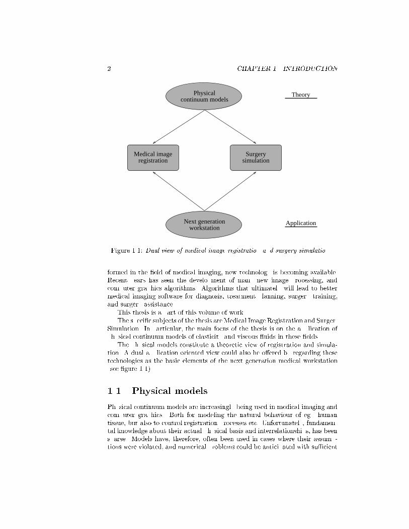
Figure 1.1: Dual view of medical image registration and surgery simulation.
formed in the eld of medical imaging, new technology is becoming available.Recent years has seen the development of many new image processing, andcomputer graphics algorithms. Algorithms that ultimately will lead to bettermedical imaging software for diagnosis, treatment planning, surgery training,and surgery assistance.
This thesis is a part of this volume of work.The specic subjects of the thesis are Medical Image Registration and Surgery
Simulation. In particular, the main focus of the thesis is on the application ofphysical continuum models of elasticity and viscous uids in these elds.
The physical models constitute a theoretic view of registration and simula-tion. A dual application oriented view could also be oered by regarding thesetechnologies as the basic elements of the next generation medical workstation(see gure 1.1).
1.1 Physical models
Physical continuum models are increasingly being used in medical imaging andcomputer graphics. Both for modeling the natural behaviour of eg. humantissue, but also to control registration processes etc. Unfortunately, fundamen-tal knowledge about their actual physical basis and interrelationships, has beensparse. Models have, therefore, often been used in cases where their assump-tions were violated, and numerical problems could be anticipated with sucient
1.2. MEDICAL WORKSTATION OF THE FUTURE 3
insight.
This thesis gives a coherent description of the basis of these models, pointingout the algorithmic weaknesses and strengths. In addition, it shows how thesemodels are the backbone of all the image registration and surgery simulationalgorithms presented in the thesis.
1.2 Medical workstation of the future
With a longer view, the algorithms and methods, described and developed in thisthesis, can be seen as some of the basic elements of the next generation medicalworkstation. A workstation, which would allow surgeons and other medical stato diagnose patients, prepare surgery, practice surgery on a virtual patient inthe workstation, and perform surgery under the guidance of the computer.
The registration techniques are essential elements of the diagnostic part ofthe workstation, providing the ability to combine multimodality images for mul-tispectral classication, and automatically segment images using atlas registra-tion. In addition, the physically based methods for surgery simulation are themain technology for creating realistic virtual surgery environments.
1.3 Thesis overview
The main structure of the thesis puts the work on medical image registrationrst, followed by the work on surgery simulation. Introductions to these eldsand reviews are given in chapters 2 and 7 respectively.
The main theoretical chapter of the thesis is chapter 4, where the physicalcontinuum elastic and viscous uid models are introduced. This chapter can beseen as the hinge of the thesis, around which most of the remaining chaptersdevelop.
The medical image registration work is described in two chapters.
In chapter 3, voxel similarity measures for rigid image registration are eval-uated. This chapter discusses the previous work, and shows that almost all ofit can be described using Grey Level Cooccurrence Matrices (GLCM). GLCMsare used in texture analysis, and a range of measures based on these matricesexists. A selection of these measures are compared to the existing voxel simi-larity measures to evaluate them for rigid medical image registration. Imagesfrom the Visible Human dataset are used for the evaluation.
After the introduction of the physical continuum models in chapter 4, chap-ter 5 discusses their application for non-rigid registration of medical images. Inparticular, a new and faster algorithm for viscous uid registration is developed.
Chapter 6 presents an alternative approach to non-rigid registration of med-ical images. It uses actual medical knowledge of the development between twoimages, to register the images non-rigidly. This chapter can be seen as a re-sponse to those people, who have criticized the use of elastic and uid modelsin non-rigid medical image registration. They have, correctly, pointed out that

4 CHAPTER 1. INTRODUCTION
the elastic and uid models are poor models of the actual physical dierence be-tween images. By implementing a computer model of the growth process of themandibular bone, this chapter shows that it is possible to register two imagesusing a correct physical model.
After the introduction to surgery simulation in chapter 7, chapter 8 describesthe development of real-time deformable models for surgery simulation usingnite element models of linear elasticity. New ways of improving the real-timeresponse of these models are presented, resulting in socalled Fast Finite Element(FFE) models.
1.4 Thesis contributions
The main contributions of this thesis are listed in this section. Since denitionsand nomenclature dened in subsequent chapters are used to keep a compactformat, the reader might want to delay reading this section initially.
The main contributions of this thesis are (in order of importance):
Fast Finite Element models These models are developed in chapter 8, andallow real-time deformation of volumetric deformable models. There arethree main contributions to the use of nite elements:
1. The use of condensation to reduce the complexity of the volumet-ric models to a complexity similar to that of a surface model (butretaining the volumetric behaviour).
2. The direct inversion of the stiness matrix of the linear matrix equa-tion resulting from the nite element model. This reduces the simu-lation time dramatically.
3. The use of static simulation instead of dynamic simulation. By ex-ploiting the sparseness of the static force vector, a considerable re-duction in computation time is achieved.
This work has been published in [BN95b, BN96c, BN96d].
Fast viscous uid registration algorithm In chapter 5 a new core algo-rithm for the viscous uid registration algorithm of Christensen et al. [Chr93,Chr94b, Chr94, Chr96] is developed. This new algorithm allows a speedupof the viscous uid registration by at least a factor of magnitude. In prac-tice, it means that the registration can be performed on a single worksta-tion instead of on a massively parallel computer.
In addition, this chapter demonstrates that the 'demon'-based registra-tion algorithm of Thirion [Thi96] is the rough simplication of the uidalgorithm.
This work will be published in [BN96e].
Growth-based non-rigid registration Chapter 6 presents a new form ofnon-rigid registration of medical images. Using the simplicity of the
1.5. CREDIT 5
growth processes of the mandibular bone, a registration algorithm fortime sequence images of the mandible is developed. This algorithm usesthe actual physical process to control the deformation from one image tothe next.
Using the actual physical process to regularize the registration process,rather than an arbitrary elastic or uid model, has not been describedbefore.
In addition, implicitly, the registration process is also the rst computermodel of the physical bone growth processes of the human mandible.
This work is being submitted.
Rigid registration using GLCM features By using the analogy with GreyLevel Cooccurrence Matrices (GLCM), features from texture analysis areidentied that could be used as voxel similarity measures for rigid imageregistration.
Several of these measures are evaluated for registration and comparedto the previously known voxel similarity measures. The experiments arecarried out using cryosection, MR, and CT images from the Visible Humandata set.
The results are mixed, but show that Mutual Information is the bestgeneral voxel similarity measure. For specic modality combinations, someof the new texture measures perform better, though.
Results of registration of CT and MR images, and cryosection and CTimages are shown. Voxel-based registration of cryosection and CT imageshas not been described before.
In addition, it is pointed out that the common scaling of rotations com-pared to translations using degrees and millimeters, respectively, is wrong.Experiments are carried out to calculate correct scaling factors.
This work is being submitted.
Description of physical continuum models The review and description inchapter 4, of the physical continuum models used in medical image regis-tration and surgery simulation, is believed to be the rst complete reviewof the theoretical aspects of the continuum models and their applicationin medical imaging.
1.5 Credit
Some of the work in this thesis has been carried out in collaboration with otherpeople. This section species their contributions.

6 CHAPTER 1. INTRODUCTION
1.5.1 Viscous uid registration
The viscous uid registration work, described in chapter 5, was initiated dur-ing my stay in the Epidaure group of INRIA. It was inspired by the work byNielsen et al. [Nie94], who showed that Thikonov regularization of a eld couldbe achieved by the simple application of a Gaussian lter, and the work byThirion [Thi96] on 'demon'-based non-rigid registration. The latter work alsoused the Gaussian lter.
I continued this work after returning to Denmark. On my initiative andunder my supervision, M.Sc. Claus Gramkow joined me during his M.Sc. thesis.Most of the software was written by Claus Gramkow.
1.5.2 Fast Finite Elements
During my stay in the Epidaure group I also developed the ideas for the FastFinite Element models. I had many discussions with Ph.D. student StephaneCotin on the basics of nite element models. Stephane Cotin implemented therst nite element models.
The three contributions listed in the section on contributions, were devel-oped by myself in Denmark. Although the use of inversion seems to have somesimilarity with the approach of Cotin et al. [Cot96], it is formulated in a dierentway.
1.5.3 Growth registration
The work on bone growth models for non-rigid registration, was strongly in-spired by discussions with Prof. Sven Kreiborg. His input, in the form ofmedical knowledge of the growth of the mandibular bone, was essential for thedevelopment of the computer models.
Chapter 2
Medical Image Registration
Segmenting medical images have turned out to be a more dicult task thanmany image processing researchers originally expected. The individual modal-ities such as x-ray Computed Tomography (CT), Magnetic Resonance (MR)imaging, Ultra Sound (US), etc., do not individually provide enough contrastand information to reliably segment all tissue types in images acquired of humanpatients.
Although much research is still being directed at improving segmentationalgorithms, the quality of the image data inherently gives a natural limit to thepossible quality of the segmentation results. Only when a limited number ofobjects or tissue classes are present in the images and the imaging process hasbeen designed to provide good contrast for these classes, is it possible to obtaingood results. Contrast is sometimes sucient in one of the normal modalities,eg. bones in CT scans, but often injection of contrast media is used to extractdesired anatomical structures.
In addition, sometimes anatomical structures are made of the same tissue ona microscopic level, and only dier in function at a macroscopic level. Eg. braintissue is very homogeneous but have very dierent function, depending on theposition in the brain. This dierence is not visible in local images of the tissueand can only be determined based on the position of the tissue in the globalstructure of the brain.
Bones are another good example of tissue where function is determined ata macroscopic level. Although they have very similar response in CT scans,they should optimally be segmented into separate structures corresponding torib, femur, vertebrae, etc. With traditional classication algorithms it is notpossible to solve this segmentation problem.
Because of these problems, much attention has been directed towards regis-tration methods in recent years (see [Bro92] for a general review of image regis-tration techniques). Image registration methods can solve some of the inherentproblems of mono-modality images and voxel-based classication algorithms.
Rigid multi-modality registration methods allow images of the same patient,but from dierent modalities, to be registered. This provides joint information
7
8 CHAPTER 2. MEDICAL IMAGE REGISTRATION
that is:
Complementary: Each modality provides dierent information. Eg. x-rayComputed Tomography (CT) provides information about bone and cal-cications, whereas Magnetic Resonance (MR) provides complementaryinformation about soft tissues.
Synergistic: The combination of two modalities may provide additional infor-mation. Eg. Positron Emission Tomography (PET) and Single PhotonEmission Computed Tomography (SPECT) provide functional images ofthe brain, but have very little information about anatomy. CombiningPET or SPECT images with MR images increases the value of the PETand SPECT images, since the precisely imaged brain structures in theMR images can be transferred to the functional images. Function can,consequently, be described in terms of anatomy.
The result is that registered images contain more information in each voxel,thus making the segmentation using standard classication algorithms easier.
Another way of introducing more information is using non-rigid registrationmethods to combine images from either time studies of the same patient ordierent patients. The latter method is often used with Positron EmissionTomography (PET) images. These images are quite noisy, and the accumulationof information from several dierent patients, allows the noise to be suppressedstatistically.
The use of registered multi-modality images only improves the local infor-mation content. The problem of segmenting anatomical structures with similarcharacteristics is more complex, and a-priori knowledge of anatomy must be putinto the segmentation process. To solve this problem, non-rigid registration offunctional and topological atlases to patients has been proposed. By mappingthe atlas onto the patient it is possible to transfer function, topology, and otherinformation from the atlas to the individual patient.
Registration of medical images has traditionally been performed using eithermanual methods or extrinsic markers. Unfortunately, these methods have se-vere disadvantages in terms of precision and/or patient discomfort (stereotacticframes). Much eort has therefore been put into development of non-invasiveretrospective image registration techniques, which are more precise and fullyautomatic. This thesis contributes to this volume of work, and emphasis istherefore put on retrospective image registration.
In this chapter an overview of the techniques used in medical image regis-tration will be presented. Since very good reviews have been published previ-ously by Brown [Bro92], Maurer and Fitzpatrick [Mau93], and Van den Elsen etal. [Els93], there is no reason to repeat this work here. We will instead try to givethe reader an understanding of the basic issues in medical image registrationand the technical factors that distinguish dierent registration methods.
There are basicly two factors that in uence the classication of medicalimage registration methods: The motion model that determines what transfor-mations are allowed and the driving potential that determines the forces driving

2.1. MOTION MODEL 9
Rigid (translation, rotation)
Elastic deformation
Free deformation
Figure 2.1: Rigid, elastic, and free motion. Left: Possible deformation of box.Right: Possible deformation of line to curve.
the motion of the images wrt. each other.
2.1 Motion model
Motion models are normally classied into either rigid or non-rigid in the com-puter vision and medical imaging literature. This text proposes an extendedclassication into three classes: Rigid, elastic, and free motion models. Al-though elastic and free motion models can be classied together as non-rigid,there are fundamental dierences in the resulting transformations they achieve.The three motion models are illustrated in gure 2.1.
2.1.1 Rigid motion
Rigid body motion is composed of a rotation followed by a translation. Thebody therefore retains its shape and form under a rigid transformation.
Extensions to the basic rigid transformation include scaling and more generalane transformations. These motion models are not used in this thesis and wetherefore ignore them.
2.1.2 Elastic motion
Transformations governed by elastic motion models allow constrained deforma-tion of images. The constraints are typicly implemented using potential energyfunctions for elastic continua, and the transformation becomes a compromise
10 CHAPTER 2. MEDICAL IMAGE REGISTRATION
between the driving forces and the restoring forces of the elastic continuum.Consequently, the driving potential never completely vanishes (see gure 2.1).
Although they never fully achieve the transformation implicitly desired bythe driving forces, these models are more robust and smooth than the freemotion models, because of the regularization eect induced by the elastic con-tinuum.
In addition to elastic transformations this group of motions also includespolynomial models. These are not used in this work.
2.1.3 Free motion
Free motion models typically allow any deformation that is well-formed. Anexample of a free motion model is uid motion. Using uid motion any defor-mation can be attained over time, but the transformation is restrained duringthe deformation process to prevent a breakdown of the well-formedness require-ment.
2.1.4 Parameter space
As the variability of these motion models increases, so does the complexity of theparameter space. Whereas rigid motion models have 6 parameters, regularizedelastic models typically have in the hundreds of parameters and uid models inthe thousands or millions of parameters. Naturally, with an increasing numberof parameters the computational complexity and time consumption increase.On the other hand with an increasing number of parameters more complexmotion is possible.
The classication of the motion models can be seen as a motion model scaleusing the number of parameters as the scale parameter. A multi-scale approachis often used for elastic and free registration where rst a rigid registration isapplied, followed by an elastic and possibly a free registration. An advantageof this approach is that it introduces a regularization eect in the registrationthat makes it more robust.
2.2 Driving potential/force
It is dicult to nd a useful classication of the possible driving potentials,since the methods often t several categories at the same time. This is alsoseen from the dierent reviews of medical image registration methods [Bro92,Mau93, Els93]. All use dierent, though related, categories.
We choose to classify the driving potentials into point, curve, surface, mo-ments and principal axes, and voxel similarity potentials. These are describednext.
2.2. DRIVING POTENTIAL/FORCE 11
2.2.1 Point methods
Point methods are used when corresponding sets of points are available in thetwo datasets. These points can either be extrinsic or intrinsic. Extrinsic pointsare typically external skin markers on the patient or markers on stereotacticframes.
Registration using markers on stereotactic frames is usually very precise.But, the discomfort to the patient, caused by the frame which is screwed intothe skull of the patient, can be quite serious. See [Mau93] for more discussionon registration using stereotactic frames and pointers to reviews.
External skin markers on the patient come in many dierent forms andmaterials (see [Mau93] for discussion of dierent marker types). A problemwith these markers is movement of the skin. But on the other hand they arerelatively easy to locate and can be designed to allow subslice/pixel precision(eg. the V shaped markers used by Van den Elsen [Els91])
Intrinsic points are typically anatomic landmarks, such as bloodvessels bifur-cations [Hi91], which are located by the physician. Location of these anatomicalpoints can be quite dicult, and the precision seldom match that of extrinsicmarkers. The advantage of the intrinsic points is their retrospective nature.Extrinsic points require that registration is planned before acquisition of theimages, since markers must be physically placed on the patient, whereas in-trinsic points are determined in the image without special requirements for theimaging process. This means that historic data (without extrinsic markers) canbe registered using intrinsic points. Hill et al. [Hi91, Hi92, Hi92b] suggestedseveral anatomic structures as intrinsic points.
Work by Thirion et al. [Thi93b] indicates that intrinsic points can be foundautomatically. They detected socalled extremal points based on invariants ofdierential geometry, and have used these points as automatically determinedanatomic registration landmarks.
Rigid registration of corresponding point data-sets can be formulated as aleast-squares problem. Several closed-form solutions exists [Mau93]: SingularValue Decomposition (SVD) [Aru87], eigenvalue-eigenvector decomposition of amatrix [Hor88] and dual quaternions [Hor87, Fau86]. Point set matching usingdual quaternions has been implemented in the software package Mvox [BN96].
Non-rigid registration of point sets has been used both for registration of twodierent images and for registration to an atlas. See [Mau93] for more details.One method for non-rigid registration of images using corresponding point sets,models one of the images as a thin-plate spline and uses the corresponding pointsto deform it. An elegant implementation is given by Bookstein in [Boo89], whichhas also been implemented in the software package Mvox [BN96].
2.2.2 Curve methods
Curves derived from intrinsic structures can be used to register images, if thesestructures are present and positioned indentically in both images.
Interesting work on this subject has been pursued at the Epidaure group

12 CHAPTER 2. MEDICAL IMAGE REGISTRATION
of INRIA. Based on extrema of curvature in the image intensity eld, theyextract characteristic geometric features [Mon92, Thi92, Thi93] which they callthe extremal mesh [Thi93b]. This mesh includes ridge/crest lines and extremalpoints.
Gueziec and Ayache smoothed the ridge lines and used a B-spline represen-tation of them to register two CT images rigidly. Thirion et al. used the crestlines for rigid registration of CT images in [Thi92b]. Declerck et al. [Dec95] andSubsol et al. [Sub95] have used the crest lines as stable features of skull anatomyand registered CT images non-rigidly to atlases. Medical applications of thistechnique were represented in [Sub96].
The limitation of the algorithm seems to be the necessity for high resolutionimages for stable extraction of the geometric features. But, work is ongoing byFidrich and Thirion [Fid94] to establish the behaviour of the extremal mesh inscale-space, ie. lower resolution.
In addition, Pennec (eg. [Pen96]) is working on statistical treatment of thegeometric features. Crest lines and extremal points are well-suited for statisticalanalysis of shape, and the application of these geometric features to probabilisticatlases is an interesting aspect.
2.2.3 Surface methods
Three popular registration methods have dominated rigid registration algo-rithms using surface information: The head-hat algorithm by Pelizarri et al. [Che88,Pel89, Lev88], the Hierarchical Chamfer Matching (HCM) algorithm, whichwere rst proposed by Borgefors [Bor88] based on initial work by Barrow etal. [Brw77], and later used for rigid registration of 3D medical images by Jianget al. [Jia92, Jia92b], and the Iterated Closest Points (ICP) algorithm by Besland Kay [Bes92].
The head-hat algorithm was developed specicly for registration of images ofthe head [Che88, Pel89, Lev88]. The surface of one of the images is used as thehead and a set of points is extracted from surface contours in the other imageto represent the hat. The hat is then registered to the head by minimizingthe distance of hat points from the head surface along a line from the pointto the centroid of the head surface. The rigid transformation parameters aredetermined by minimizing the distance energy using Powell's algorithm [Pow64].
In the Hierarchical Chamfer Matching (HCM) algorithm, a chamfer distancemap (thus the name) is generated from the surface of one of the images [Bor88,Jia92, Jia92b]. This distance map is used as a potential function for surfacepoints in the other image and the total potential is minimized to nd the rigidregistration parameters.
Instead of using the surface of the image objects, Van den Elsen et al. [Els92]proposed using geometric features extracted from the images using dierentialgeometry. Van den Elsen et al. applied this to registration of MR and CTimages.
The Iterated Closest Points (ICP) algorithm was introduced by Besl andKay [Bes92], and later algorithmicly improved by Zhang [Zha94] by the use
2.2. DRIVING POTENTIAL/FORCE 13
of k-D trees, as suggested for future work by Besl and Kay. Images must berepresented using points on the surface for this algorithm. In each iteration ofthe algorithm, the closest point in one image is determined for all points in theother image. These point correspondences are used to register the images usingclosed-form point registration methods as described in section 2.2.1.
The Epidaure group at INRIA has used this algorithm extensively for rigid,ane and locally ane registration (Feldmar and Ayache [Fel94]), and rigid,ane and local spline registration (Declerk et al. [Dec96]). In addition Collignonet al. was inspired by the algorithm in [Col93b].
Rigid registration of 3D surfaces using the ICP algorithm has been imple-mented in the software package Mvox [BN96].
Szeliski and Lavallee have suggested an alternative representation of thesurfaces and their deformation [Sze94]. Using an octree-approximation of thedistance potential eld and an octree-spline deformation eld they registeredsurfaces non-rigidly.
Other non-rigid surface registration work include that of Moshfeghi et al.,who have extended the 2D work by Burr [Bur81] to 3D for non-rigid registrationof surface contours [Mos94].
2.2.4 Moments and principal axes methods
With the moments and principal axes methods, image objects are modeled asellipsoidal point distributions. Such distributions can be described using therst and second moments of the point positions. Registration is performed byoverlaying the centroids of the objects, and aligning the principal axes, whichare determined by the eigen-vectors of the covariance matrix. Scaling can bedetermined from the eigen-values of the covariance matrix.
These methods have been widely used for registration of medical images[Alp90, Ara92, Fab88, GA86]. Unfortunately, a major limitation of the momentsand principal axes methods is the high sensitivity to shape dierences. Missingdetails or pathology can severely distort the registration results. They are,therefore, mostly used as a rough initial registration step, eg. [Baj89, BN96e].
2.2.5 Voxel similarity methods
Voxel similarity methods register images based on all the voxels in the images.They are therefore, generally robust and results can be quite exact. On theother hand, they have a high computational complexity, and it is only in recentyears that practical applications of these methods have turned up.
In this thesis the focus of the registration work is on voxel similarity basedmethods, and reviews of existing work are therefore giving in the respectivechapters. See chapters 3 and 5 for rigid and non-rigid registration methodsrespectively. In addition see the next section on electronic atlases.
14 CHAPTER 2. MEDICAL IMAGE REGISTRATION
2.3 Registration to electronic atlases
An important application of non-rigid registration methods is registration ofimages to an electronic atlas. Precise registration allows syntactic and semanticinformation from the atlas to be transferred to individual patient images.
The immediate application is of course automatic segmentation of images,by transferring the topological information, implicitly stored in the atlas, tothe patient. Other information that could be transferred include functional,relational, and hierarchical information.
Another application of registration to an atlas is accumulation of data fromimages of many patients. This is used in functional imaging, where eg. PETactivation images from many patients are registered to the same reference frame,to allow statistical treatment of the functional information.
In PET imaging, the Talairach atlas [Tal88] has often been used as such areference frame. Patient images are mapped to the atlas by piecewise anetransformations [Eva92, Fox85, Ge92, Lem91]. Although the mapping is roughthis approach has been widely used.
Other atlases include the pioneering VoxelMan atlas by Hoehne et al. [Hoe92,Hoe92b, Hoe94]. This atlas has set a standard in visualization and manipula-tion of anatomical data. It includes both the original modalities (CT/MR) aswell as functional, topologic and hierarchic information, thus allowing the userliterally to point out regions of a 3D brain and ask 'what is that' or 'what isthis part of'.
The development of the Visible Human/Woman [Vis96] data set is anothermilestone in electronic atlases. Although it has not been completely segmented(or registered), this data set covers the entire body with CT, MR, and RGBcryosection images of histological slices. Several groups are currently workingon electronic atlases based on this data set, eg. [Ker96, Tie96].
The algorithms for registration of images to an atlas, can be classied basedon the level of human intervention in the registration process.

2.4. SUMMARY 15
Manual alignment of image to atlas: Fox et al. [Fox85] and Evans et al. [Eva88]registered images manually to an atlas by performing a rigid or anetransformation followed by nonlinear scaling. Greitz et al. [Gre91] alsoused manual registration using rigid transformations, but followed this bya small set of non-rigid transformations.
Supervised alignment of image to atlas: These methods are all based onregistration using landmarks. Bajcsy et al. [Baj88], Pelizzari et al. [Pel89],and Undrill et al. [Und92] registered the images using rigid transformationsfollowed by scaling. Undrill also allowed non-rigid boundary registration.Bookstein et al. [Boo92] and Evans et al. [Eva91] used thin-plate splinemodels to elasticly warp the images based on the landmark correspon-dences.
Automatic alignment of image to atlas: Both Bajcsy et al. [Baj89, Gee93]and Collins et al. [Cli92] used cross-correlation to drive the non-rigid reg-istration. Both groups regularized the deformation by using a multires-olution framework, but Bajcsy et al. also modeled the image as a linearelastic object. Bajcsy et al. were the rst to introduce physical continuummodels to the problem of voxel-based non-rigid image registration.
Instead of using a multiresolution framework to regularize the registrationprocess, Miller et al. [Mil93, Chr94] used a limited set of eigen-functionsof the linear elastic model. This was rst applied followed by registrationwith a full linear elastic model.
In later work Christensen et al. have used viscous uid continuum modelsinstead of the elastic models, to obtain a more exible registration, andalso to avoid mathematical problems associated with the linear elasticmodel [Chr93, Chr94b, Chr94c, Chr96].
Subsol et al. [Sub95] used crest lines as the driving potential and registeredimages to a skull atlas using parametric modal elastic models.
The development of these models has proceeded from manual semi-rigid meth-ods over elastic and parametric/polynomial models to the free registration meth-ods dened by uids. The uid models have unfortunately not been used byother groups than Christensen et al., because of the previous enormous com-putational complexity of the solution problem. In this thesis a new algorithmfor uid registration is proposed, which is considerably faster than the originaland, therefore, progress can hopefully be expected with these models.
2.4 Summary
This chapter have presented a review of the most important techniques in med-ical image registration. Image registration is a wide eld and many techniqueswere described. The following chapters will present new work in voxel-basedrigid registration, free uid registration, and free growth-based registration.

16 CHAPTER 2. MEDICAL IMAGE REGISTRATION

Chapter 3
Rigid Registration using
Voxel Similarity Measures
In this chapter, we will concentrate on rigid registration of medical images usingvoxel similarity measures. An advantage of the voxel-based registration methodspresented in this chapter, is the fact that they are fully automatic and requireno pre-processing of the images, as do eg. the surface registration methodsmentioned in the previous chapter.
The main part of the chapter discusses existing and some new voxel sim-ilarity measures. Elaborate tests are used to evaluate the dierent measuresand compare them. Finally, a registration algorithm based on voxel similaritymeasures is described and some results are presented.
3.1 Image data
The algorithms developed in this chapter have been applied to registration ofimages from the Visible Human data set [Vis96]. From this data set, images ofthe head from the following modalitites have been used (see gure 3.1):
MR, Proton Density weighted (PD)
MR, T1 weighted (T1)
CT, windowed for bone (CT)
Red channel of the cryosection colour image (R)
These images were taken from the Research Systems' Visible Human CD.Using a combination of manual and automatic tools the images were reg-
istered to each other to get an initial ground truth. This registration wasperformed carefully using visual inspection for validation of the results. Un-fortunately, during this registration process, the voxel size of the MR images
17
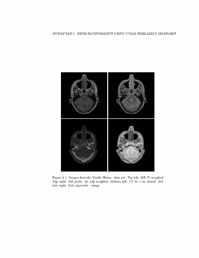
18CHAPTER 3. RIGID REGISTRATIONUSING VOXEL SIMILARITYMEASURES
Figure 3.1: Images from the Visible Human data set. Top left: MR T1 weighted.Top right: MR proton density weighted. Bottom left: CT bone windowed. Bot-tom right: Red cryosection image.

3.2. VOXEL SIMILARITY MEASURES 19
turned out to be inconsistent with the size of the other images. By measuringthe distance between anatomical landmarks the voxel size were estimated to 1.05x 1.05 x 5 mm instead of 1.016 x 1.016 x 5 mm as given in the documentationfor the MR images.
The following combinations of modalities are explored in this chapter: PD/T1,CT/T1, and CT/R. PD/T1 is only used to show the basic behaviour of the sim-ilarity measures and registration results for this combination are consequentlynot reported. Voxel-based registration of CT and cryosection images has notbeen documented before.
3.2 Voxel similarity measures
For registration of uni-modal images, correlation has been used extensively inboth remote sensing, medical imaging and other application areas.
Simple correlation of grey-values assumes that a linear relationship betweenthe grey-values exists [Bro92]. This is seldom the case, and grey-level correlationhas, therefore, not provided convincing results for multi-modality registrationof images.
In recent years, though, renewed interest in voxel-based multi-modality reg-istration has been revived by the successful work on PET/PET and PET/MRregistration by Woods et al. [Woo92, Woo93]. The basic assumption of thiswork is the same as for correlation, ie. that a linear mapping exists betweengrey-values g1 and g2 of the two images. As mentioned above, this assumptionis seldom valid for multi-modality images. But Woods et al. circumvent thisproblem by looking instead at the variance of the coecient R = g1=g2, whereg1 is the PET image grey-value. They argue that this coecient of variationis minimized when the images are in register, and have achieved good resultsfor PET/PET registration [Woo92] using this measure. For PET/MR regis-tration they have proposed a modied version of the initial measure [Woo93],where the variance is calculated independently for each MR grey-value and sub-sequent summed weighted by the probability estimate of the MR grey-values.To achieve successful registration, only the intracranial structures are used inthe registration process, and this algorithm, therefore, needs some manual seg-mentation to work. But, the coecient of variation is today probably the bestmeasure for registration of PET/PET and PET/MR [Wes96].
Inspired by this work, Hill et al. proposed a modied algorithm for registra-tion of CT/MR in [Hi93, Hi93b]. In this algorithm CT is used as the denomi-nator g2, and only certain ranges of CT intensities are used in the calculationof the resulting coecient.
In [Hi93] Hill also proposed an alternative measure based on the third ordermoment of the 2D histogram created from the images. This was inspired byintensive studies of the development of the 2D histograms for changing registra-tion parameters. A general observation was that intensity concentrations in thehistograms seemed to disperse when the registration deviated from an optimalregistration.
20CHAPTER 3. RIGID REGISTRATIONUSING VOXEL SIMILARITYMEASURES
Van den Elsen has proposed a modied correlation approach for CT/MR reg-istration [Els94, Els94b, Els95], where the images are pre-processed to extractsimilar structures in both modalities, typicly bones. In [Els94, Els95] these struc-tures were extracted using complex dierential operators in scale-space. Similarresults were later obtained using simple ramp intensity remapping in [Els94b].
At this point all the measures proposed for multi-modality registration hadbeen based on heuristics. Several groups independently realized that the in-trinsic problem of registering two independent image modalities, could be castin an information theoretic framework. Collignon et al. [Col95] and Studholmeet al. [Stu95] both suggested using the joint entropy of the combined imagesas a registration potential, and Collignon et al. [Col95b], and Wells and Vi-ola [Vio95, Wel96] nally suggested the relative entropy or mutual informationas a registration measure. Mutual information is more robust to truncationof images than joint entropy, and has been applied to other registration tasksthan medical imaging. It is a very general measure of correspondence betweentwo images, and in a recent evaluation of a range of dierent multi-modalityregistration methods [Wes96], mutual information was quite succesful.
It turns out that most of the proposed voxel similarity measures have acorrespondence in the eld of texture analysis. This chapter shows this cor-respondence and compares the standard voxel similarity measures to measuresused in texture analysis.
3.2.1 GLCM matrices
Except for the work of Van den Elsen [Els94, Els94b, Els95] all the voxel simi-larity measures introduced above can be formulated based on the 2D histogramor joint probability distribution of the two images.
A similar family of measures is found in the texture analysis literature onGrey Level Cooccurrence Matrices (GLCM) [Cnr80, Cnr84, Har73, Har79]. TheGLCM is determined as the 2D plot of grey-values of voxels in an image with axed displacement between them.
Let g(x) be the grey-value of the pixel at position x = [x1; x2; x3]T in the
image, and let u = [u1; u2; u3]T be the displacement vector between corre-
sponding voxels. The GLCM is generated by accumulating the grey-value pairs[g(x); g(x + u)] in a 2D histogram for all image positions x. The normalizedGLCM can be seen as an estimate of the joint probability distribution of voxelsg(x) and g(x+ u).
By extending the denition of the displacement vector u to be, not onlybetween voxels in one image, but also between voxels in dierent images, theGLCM turns out to be the 2D histogram of voxel intensities used by Hill etal. [Hi93, Hi93b, Hi94c], and the normalized GLCM becomes an estimate of thejoint probability distribution of voxels in the two images.
In the GLCM texture analysis literature a range of dierent measures exists.On the following pages we evaluate these measures as voxel similarity measuresfor multi-modality image registration, and compare them to the existing voxelsimilarity measures.
3.2. VOXEL SIMILARITY MEASURES 21
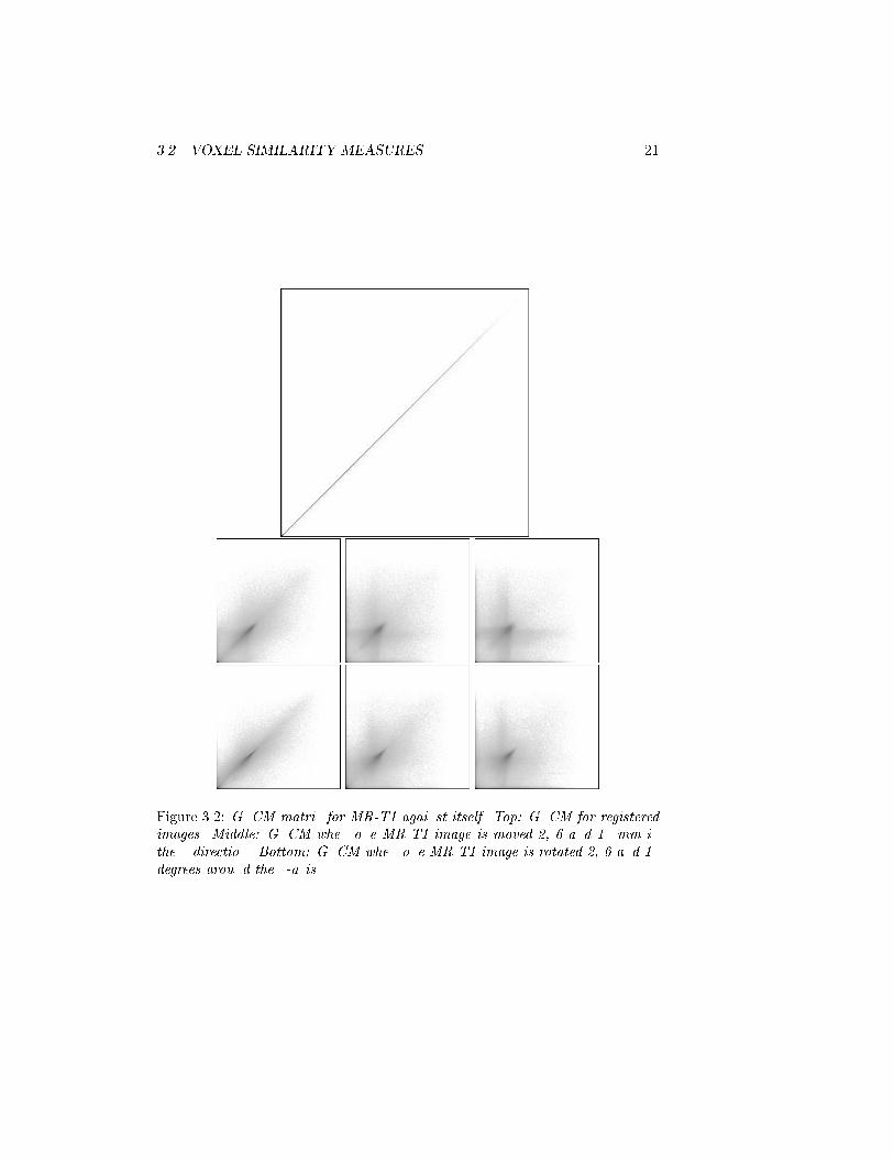
Figure 3.2: GLCM matrix for MR-T1 against itself. Top: GLCM for registeredimages. Middle: GLCM when one MR-T1 image is moved 2, 6 and 15 mm inthe x-direction. Bottom: GLCM when one MR-T1 image is rotated 2, 6 and 15degrees around the x-axis.
22CHAPTER 3. RIGID REGISTRATIONUSING VOXEL SIMILARITYMEASURES
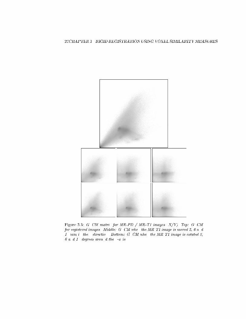
Figure 3.3: GLCM matrix for MR-PD / MR-T1 images (X/Y). Top: GLCMfor registered images. Middle: GLCM when the MR-T1 image is moved 2, 6 and15 mm in the x-direction. Bottom: GLCM when the MR-T1 image is rotated 2,6 and 15 degrees around the x-axis.
3.2. VOXEL SIMILARITY MEASURES 23
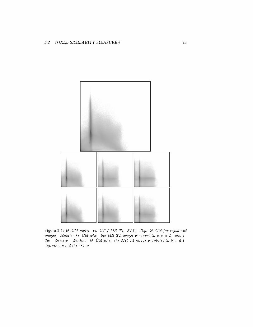
Figure 3.4: GLCM matrix for CT / MR-T1 (X/Y). Top: GLCM for registeredimages. Middle: GLCM when the MR-T1 image is moved 2, 6 and 15 mm inthe x-direction. Bottom: GLCM when the MR-T1 image is rotated 2, 6 and 15degrees around the x-axis.
24CHAPTER 3. RIGID REGISTRATIONUSING VOXEL SIMILARITYMEASURES
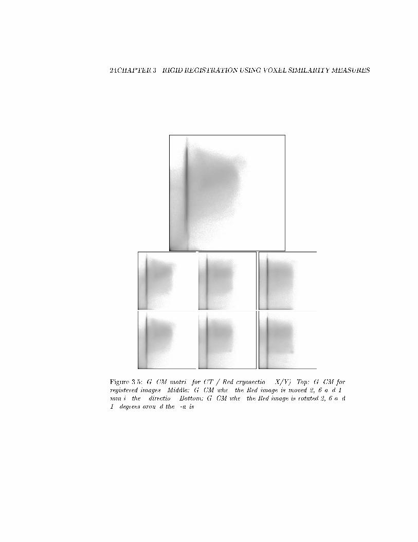
Figure 3.5: GLCM matrix for CT / Red cryosection (X/Y). Top: GLCM forregistered images. Middle: GLCM when the Red image is moved 2, 6 and 15mm in the x-direction. Bottom: GLCM when the Red image is rotated 2, 6 and15 degrees around the x-axis.
3.2. VOXEL SIMILARITY MEASURES 25
The GLCM for two identical images (T1/T1) is shown in the top of gure 3.2.As would be expected, the GLCM shows a diagonal line since identical grey-values have been plotted against each other.
In the lower part of gure 3.2 the evolution of the GLCM is displayed fortranslation in the x-direction and rotation around the x-axis. The followinggeneral observations can be made: With increasing mis-registration,
diagonal features are dispersed,
peaks are smoothed out,
lines parallel to the axes appear.
When the images are in register, grey-values in one image tend to map to alimited range of grey-values in the other image, corresponding to the grey-values of the particular anatomical structures which they both represent. Linesoccur since the range of grey-values is contaminated by grey-values from otheranatomical structures, when the images are mis-registered. This way each grey-value ends up being mapped to a large range of grey-values in the other image.
Figures 3.3, 3.4 and 3.5 show the characteristics and evolution of the GLCMfor the other combinations of modalities. Note, how the GLCMs associatedwith the CT image have a strong vertical line. This line occurs, because CThas poor contrast for the corresponding tissue type. Since both MR and the redcryosection images have better contrast for this tissue, the CT grey-values aremapped to a wide range of grey-values.
From these GLCMs, the characteristics of the CT/T1 and CT/R registrationcould be interpreted to be very similar. But this is not the case when featuresare calculated from the GLCMs and caution should, therefore, be taken whenthey are interpretated.
3.2.2 GLCM features
In the literature approximately 20 GLCM features appear which can be usedto extract information from cooccurrence matrices. Most of these features arederived by weighting the entries of the GLCM with a weighting function andsumming the result. Here a limited number of features are investigated. Thesefeatures fall in three classes based on the character of the weighting function.
Using the notation P (i; j) for elements of the normalized GLCM, the generalform of the GLCM features is:
F =Xi;j
w(i; j)P (i; j) (3.1)
where the weighting function w depends either on the normalized GLCM valueP (i; j), the spatial position in the GLCM (i; j), or both:
w(i; j) =
8<:
f(P (i; j))f(i; j)f(i; j; P (i; j))
(3.2)
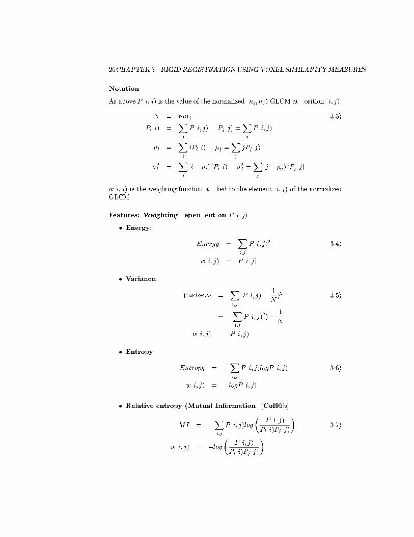
26CHAPTER 3. RIGID REGISTRATIONUSING VOXEL SIMILARITYMEASURES
Notation
As above P (i; j) is the value of the normalized (ni; nj) GLCM at position (i; j).
N = ninj (3.3)
Pi(i) =Xj
P (i; j) Pj(j) =Xi
P (i; j)
i =Xi
iPi(i) j =Xj
jPj(j)
2i =Xi
(i i)2Pi(i) 2j =
Xj
(j j)2Pj(j)
w(i; j) is the weighting function applied to the element (i; j) of the normalizedGLCM.
Features: Weighting dependent on P (i; j)
Energy:
Energy =Xi;j
P (i; j)2 (3.4)
w(i; j) = P (i; j)
Variance:
V ariance =Xi;j
(P (i; j) 1
N)2 (3.5)
= (Xi;j
P (i; j)2) 1
N
w(i; j) P (i; j)
Entropy:
Entropy = Xi;j
P (i; j)logP (i; j) (3.6)
w(i; j) = logP (i; j)
Relative entropy (Mutual Information) [Col95b]:
MI = Xi;j
P (i; j)log
P (i; j)
Pi(i)Pj(j)
(3.7)
w(i; j) = log
P (i; j)
Pi(i)Pj(j)
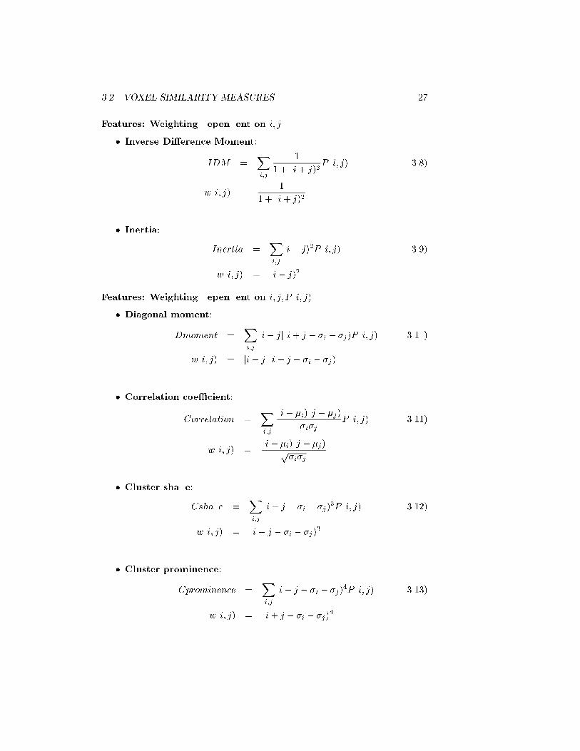
3.2. VOXEL SIMILARITY MEASURES 27
Features: Weighting dependent on i; j
Inverse Dierence Moment:
IDM =Xi;j
1
1 + (i+ j)2P (i; j) (3.8)
w(i; j) =1
1 + (i+ j)2
Inertia:
Inertia =Xi;j
(i j)2P (i; j) (3.9)
w(i; j) = (i j)2
Features: Weighting dependent on i; j; P (i; j)
Diagonal moment:
Dmoment =Xi;j
ji jj(i+ j i j)P (i; j) (3.10)
w(i; j) = ji jj(i+ j i j)
Correlation coecient:
Correlation =Xi;j
(i i)(j j)
ijP (i; j) (3.11)
w(i; j) =(i i)(j j)p
ij
Cluster shade:
Cshade =Xi;j
(i+ j i j)3P (i; j) (3.12)
w(i; j) = (i+ j i j)3
Cluster prominence:
Cprominence =Xi;j
(i+ j i j)4P (i; j) (3.13)
w(i; j) = (i+ j i j)4
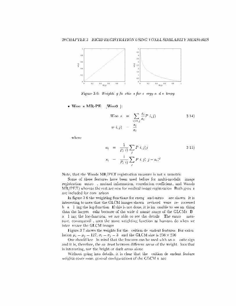
28CHAPTER 3. RIGID REGISTRATIONUSING VOXEL SIMILARITYMEASURES
0
0.2
0.4
0.6
0.8
1
0 0.2 0.4 0.6 0.8 1
w(i
,j)
P(i,j)
0
0.5
1
1.5
2
2.5
3
3.5
4
4.5
5
0 0.2 0.4 0.6 0.8 1
w(i
,j)
P(i,j)
Figure 3.6: Weighting functions for energy and entropy.
Woods MR-PET [Woo93]:
Woods =Xi>0;j
siaiP (i; j) (3.14)
w(i; j) =siai
where
ai =1
Pi(i)
Xj
P (i; j)j (3.15)
si =1
Pi(i)
Xj
P (i; j)(j ai)2
Note, that the Woods MR/PET registration measure is not symmetric.
Some of these features have been used before for multi-modality imageregistration (entropy, mutual information, correlation coecient, and WoodsMR/PET) whereas the rest are new for medical image registration. Both groupsare included for comparison.
In gure 3.6 the weighting functions for energy and entropy are shown. It isinteresting to note that the GLCM images shown previously were pre-processedby applying the log-function. If this is not done, it is impossible to see anythingthan the largest peaks because of the wide dynamic range of the GLCMs. Byapplying the log-function, we are able to see the details. The entropy mea-sure, consequently, uses the same weighting function as humans do when weinterpretate the GLCM images.
Figure 3.7 shows the weights for the position dependent features. For calcu-lation i = j = 127, i = j = 30 and the GLCM size is 256 256.
One should keep in mind that the features can be used with an opposite signand it is, therefore, the contrast between dierent areas of the weight plots thatis interesting, not the bright or dark areas alone.
Without going into details, it is clear that the position dependent featureweights cover most general congurations of the GLCM space.
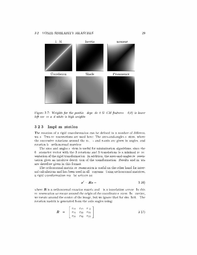
3.2. VOXEL SIMILARITY MEASURES 29
IDM Inertia Dmoment
Correlation Shade Prominence
Figure 3.7: Weights for the position dependent GLCM features. (0,0) is lowerleft corner and white is high weights.
3.2.3 Implementation
The rotation of a rigid transformation can be dened in a number of dierentways. Two representations are used here: The axes-and-angles system, wherethe successive rotations around the x-, y- and z-axis are given in angles, androtation by orthonormal matrices.
The axes-and-angles system is useful for minimization algorithms, since the6 parameter vector with the 3 rotations and 3 translations is a minimal repre-sentation of the rigid transformation. In addition, the axes-and-angles represen-tation gives an intuitive description of the transformation. Results and inputsare therefore given in this format.
The orthonormal matrix representation is useful on the other hand for inter-nal calculations and has been used in all programs. Using orthonormal matrices,a rigid transformation may be written as:
x0 = Rx+ t (3.16)
where R is a orthonormal rotation matrix and t is a translation vector. In thisrepresentation we rotate around the origin of the coordinate system. In practice,we rotate around the center of the image, but we ignore that for simplicity. Therotation matrix is generated from the axis-angles using:
R =
24 r11 r12 r13
r21 r22 r23r31 r32 r33
35 (3.17)
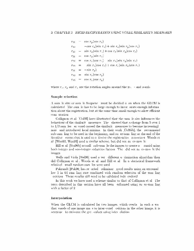
30CHAPTER 3. RIGID REGISTRATIONUSING VOXEL SIMILARITYMEASURES
r11 = cos(ry)cos(rz)
r12 = cos(rx)sin(rz) + sin(rx)sin(ry)cos(rz)
r13 = sin(rx)sin(rz) + cos(rx)sin(ry)cos(rz)
r21 = cos(ry)sin(rz)
r22 = cos(rx)cos(rz) + sin(rx)sin(ry)sin(rz)
r23 = sin(rx)cos(rz) + cos(rx)sin(ry)sin(rz)
r31 = sin(ry)r32 = sin(rx)cos(ry)
r33 = cos(rx)cos(ry)
where rx, ry and rz are the rotation angles around the x-, y- and z-axis.
Sample selection
A sample size or sample frequency must be decided upon when the GLCM iscalculated. The sample has to be large enough to incorporate enough informa-tion about the registration, but at the same time small enough to allow ecientcomputation.
Collignon et al. [Col95] have illustrated that the sample size in uences thebehaviour of the similarity measures. They showed that a change from 3 over 1to 1/3 samples per voxel caused the similarity measures to become increasinglynoisy and introduced local minima. In their work [Col95b], they recommendsub-sampling to be used in the beginning, and super-sampling at the end of theiterative process that is used to optimize the registration parameters. Woods etal. [Woo92, Woo93] used a similar scheme, but did not super-sample.
Hill et al. [Stu96b] actually sub-sample the images to create a pyramid usingboth integer and non-integer reduction factors. They did not super-sample theimages.
Wells and Viola [Wel96] used a very dierent optimization algorithm thandid Collignon et al., Woods et al. and Hill et al. In a statistical frameworkrelatively small random samples were used.
Pokrandt [Pok96] has reported preliminary good results using an extremelylow 1 in 64 sampling rate combined with random selection of the samplingpositions. These results still need to be validated independently.
In this work we have used a scheme similar to that of Collignon et al. Thetests described in this section have all been performed using super-samplingwith a factor of 2.
Interpolation
When the GLCM is calculated for two images, which overlap in such a waythat voxels of one image maps to inter-voxel positions in the other image, it isnecessary to estimate the grey-values using interpolation.
3.2. VOXEL SIMILARITY MEASURES 31
Hill et al. and Van den Elsen et al. [Hi94c, Els95] used tri-linear interpolationas the best interpolation method, when computational complexity and qualityof the results were weighted.
Collignon et al. [Col95b] recommended trilinear partial volume distributionto be used. Instead of using the interpolated grey-value to index the GLCM,they add the partial volume of each of the closest 8 voxels to the GLCM usingthe grey-values of the original voxels. The advantage should be that no newgrey-values are introduced in the images, thus minimizing noise.
For initial runs, nearest neighbour interpolation is recommended in [Col95,Hi94c].
Hill et al. [Hi94b] discusses the use of sinc interpolation and Studholme[Stu96b] comments on using a Gaussian lter, but these interpolation methodshave not been used in practice, except in the discussion in [Hi94b].
In this work tri-linear interpolation is used.
Probability estimation
The joint probability P (i; j) is estimated from the GLCM. For 12-bit imagesthe raw GLCM contains 4096 4096 bins which is bigger than some images.A reduction of the number of bins is therefore necessary to allow ecient com-putation. Parzen-windowing could be used to estimate stable probability es-timates [Du73]. But Parzen windowing is computationally expensive. Insteadall authours use binning which can be considered a crude approximation ofparzen-windowing [Col95b].
In practice the integer grey-values are binarily shifted an appropriate numberof bits. Binning is used here.
3.2.4 Plotting GLCM features
In [Hi94b, Hi94c] Hill et al. used socalled similarity measure plots to determinethe quality of voxel similarity measures. These plots show curves for displace-ments in the dierent directions, and rotations around the three axes under theassumption that the other parameters are zero.
Obviously this kind of plot does not provide any information about thequality of the measures for deviations where several parameters are non-zero.In addition, these plots do not allow quantitative evaluation of the measuresand objective comparison is not easy. On the other hand they do tend to give agood impression of the behaviour of the measures in terms of local minima andprecise localization.
In the following the measures are evaluated using two types of plots:
The similarity measure plot that Hill et al. have used. The similarity mea-sure is determined for a sequence of deviations with a single parameterat a time. This gives a curve for each parameter and these curves arecombined in a single plot.

32CHAPTER 3. RIGID REGISTRATIONUSING VOXEL SIMILARITYMEASURES
Distance/Feature plots. For a large number of random displacements, thelength of the parameter vector is plotted against the feature. It turns outthat these plots are reasonably linear for good similarity measures. Wetherefore choose the linearity as an objective measure of the feature qual-ity. Linear regression [Con84] is used to determine the best approximatingline (using the Splus software package) and the R2 is used as a qualitymeasure.
Correcting for wrong scaling of rotation
When the length of the parameter vector is determined, an implicit choice ofscaling for the rotation parameters, compared to the translation parameters, hasto be made. The obvious choice is using millimeters for translations and degreesfor rotations. In the medical image registration literature this has been usedwidely (if not exclusively), eg. [Col95b, Els95, Hi94c]. There is no theoreticalbasis for this choice and any other could just as well have been used. Work inthis chapter indicates that it is often wrong.
For algorithms that use a brute-force approach to determine the minimumof the similarity function [Els95, Hi94c] this has little in uence. But wheremore advanced methods such as Newton-Raphson [Woo92, Woo93] or Powell'smethod [Col95b] are used, dierent scaling of the rotation and translation axescan in uence the direction of steps or stop-requirements. For calculation of thedistance/feature plots the scaling also has an eect. It is therefore necessary toestimate the correct scaling.
Two distance/feature plots are created, where one uses only rotation andthe other only translation in the parameter vector. Using linear regression,approximating lines are determined for these two plots. Assuming that theestimates of the slopes of the lines are rot and tr for rotation and translation,respectively, a correction factor is determined as:
rot2tr =rotrtr
(3.18)
This correction factor is pre-multiplied all rotation parameters before the lengthof the parameter vector is determined. Using corrected rotation parameters,a nal distance/feature plot is calculated where all parameters take randomvalues.
3.2.5 Results
In appendix D the entire set of plots is shown. The linear regression results forthe distance/feature plots are listed along with calculated correction values andR2 for the corrected and uncorrected plots.
The similarity measure plots call for a subjective evaluation and we haveperformed this evaluation using the following scale:
1. Useless,
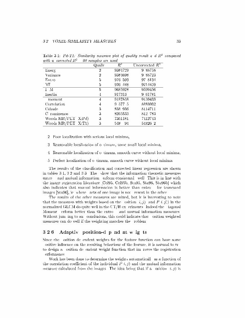
3.2. VOXEL SIMILARITY MEASURES 33
Table 3.1: Pd-T1: Similarity measure plot of quality result and R2 comparedwith uncorrected R2. 500 samples are used.
Quality R2 Uncorrected R2
Energy 2 0.9384729 0.9088758Variance 2 0.9384698 0.9088723Entropy 5 0.9760593 0.9708134MI 5 0.9260448 0.9214459IDM 5 0.9685928 0.9599456Inertia 4 0.9173130 0.9061781Dmoment 4 0.9187858 0.9159433Correlation 4 0.9057705 0.8883932Cshade 3 0.8380936 0.8114711Cprominence 3 0.8265533 0.8120783Woods MR/PET (X:Pd) 3 0.7361181 0.7412743Woods MR/PET (X:T1) 3 0.5480094 0.5482602
2. Poor localization with serious local minima,
3. Reasonable localization of optimum, some small local minima,
4. Reasonable localization of optimum, smooth curve without local minima,
5. Perfect localization of optimum, smooth curve without local minima.
The results of the classication and corrected linear regression are shownin tables 3.1, 3.2 and 3.3. They show that the information theoretic measuresentropy and mutual information perform consistently well. This is in line withthe image registration literature [Col95, Col95b, Stu95, Stu96, Stu96b] whichalso indicates that mutual information is better than entropy for truncatedimages [Stu96], ie. where parts of one image is not present in the other.
The results of the other measures are mixed, but it is interesting to notethat the measures with weights based on the position (i; j) (and P (i; j)) in thenormalized GLCM do quite well in the CT/R experiments. Indeed the DiagonalMoment perform better than the entropy and mutual information measures.Without jumping to any conclusions, this could indicate that position weightedmeasures can do well if the weighting matches the problem.
3.2.6 Adaptive position-dependent weights
Since the position dependent weights for the feature function can have somepositive in uence on the resulting behaviour of the feature, it is natural to tryto design a position dependent weight function that improves the registrationperformance.
Work has been done to determine the weights automatically as a function ofthe correlation coecient of the individual P (i; j) and the mutual informationmeasure calculated from the images. The idea being that if a position (i; j) is

34CHAPTER 3. RIGID REGISTRATIONUSING VOXEL SIMILARITYMEASURES
Table 3.2: CT/T1: Similarity measure plot quality results and R2 compared withuncorrected R2. 500 samples are used.
Quality R2 Uncorrected R2
Energy 4 0.9505296 0.9493070Variance 4 0.9505302 0.9493080Entropy 5 0.9666757 0.9638251MI 4 0.8077108 0.7595025IDM 2 0.9416978 0.9384330Inertia 1 0.6917992 0.6948765Dmoment 1 0.2931991 0.2798332Correlation 1 0.5524907 0.5277128Cshade 1 0.0773453 0.0773202Cprominence 1 0.3667449 0.3952463Woods MR/PET (X:CT) 4 0.6376055 0.6018653Woods MR/PET (X:T1) 4 0.8147630 0.8139735
Table 3.3: CT/R: Similarity measure plot quality results and R2 compared withuncorrected R2. 500 samples are used.
Quality R2 Uncorrected R2
Energy 1 0.4335973 0.3803990Variance 1 0.4335405 0.3803409Entropy 5 0.9801963 0.9790247MI 4 0.9016652 0.8648146IDM 3 0.9476440 0.9375267Inertia 5 0.9721051 0.9725199Dmoment 5 0.9896430 0.9720567Correlation 4 0.9176131 0.8917624Cshade 4 0.8500580 0.7844821Cprominence 4 0.8491666 0.7947552Woods MR/PET (X:R) 3 0.7792640 0.7764421Woods MR/PET (X:CT) 2 0.9013030 0.8753324
3.3. IMAGE REGISTRATION USING VOXEL SIMILARITY MEASURES35
important for the similarity measure, P (i; j) should be strongly correlated withthe MI measure.
Unfortunately, it was not possible to obtain better results using the adaptiveweight calculation and this work is consequently not reported here.
3.3 Image registration using voxel similarity mea-sures
A registration algorithm similar to that of Collignon et al. [Col95b] has been im-plemented. The method optimizes the registration using Powell's algorithm foroptimization without derivatives [Pow64]. Multi-resolution is used to speedupthe algorithm.
A Quasi-Newton algorithm was tested, but problems calculating stable esti-mates of the rst derivatives caused the results to be somewhat poor.
All the voxel similarity measures may be used for the registration. But inpractice we have preferred the mutual information most of the time, since itprovides consistent results for dierent modalities.
The result of the 3D registration of the MR T1 weighted image to the CTbone windowed image using mutual information, is shown in gures 3.8, 3.9and 3.10. The 3D registration of the Red channel of the cryosection image tothe CT bone windowed image is shown in gures 3.11, 3.12 and 3.13.
Results of the registration could only be validated by visual inspection andexhaustive test were therefore not performed. But the visual inspection of theresults showed that the registration was quite precise.
3.4 Summary
In this section voxel similarity measures for registration of the Visible Humandata set have been explored.
The 2D histogram of joint voxel intensities, used in the literature as a basisfor denition of many voxel similarity measures, was shown to be similar to theGLCM matrices used in texture analysis of images.
A range of features from texture analysis were compared to the state-of-the-art features. This comparison showed that the state-of-the-art features entropyand mutual information were best for general registration, since they performedconsistently well for both registration of MR-T1 to MR-PD, MR-T1 to CT bone,and red cryosection to CT bone. For each of the other combinations, some of thetexture measures were at least as good as the information theoretic measures.But, these results were not consistent from one modality combination to thenext.
Together with the information from the literature, this leads to the conclu-sion that mutual information is the best generally applicable voxel similaritymeasure.
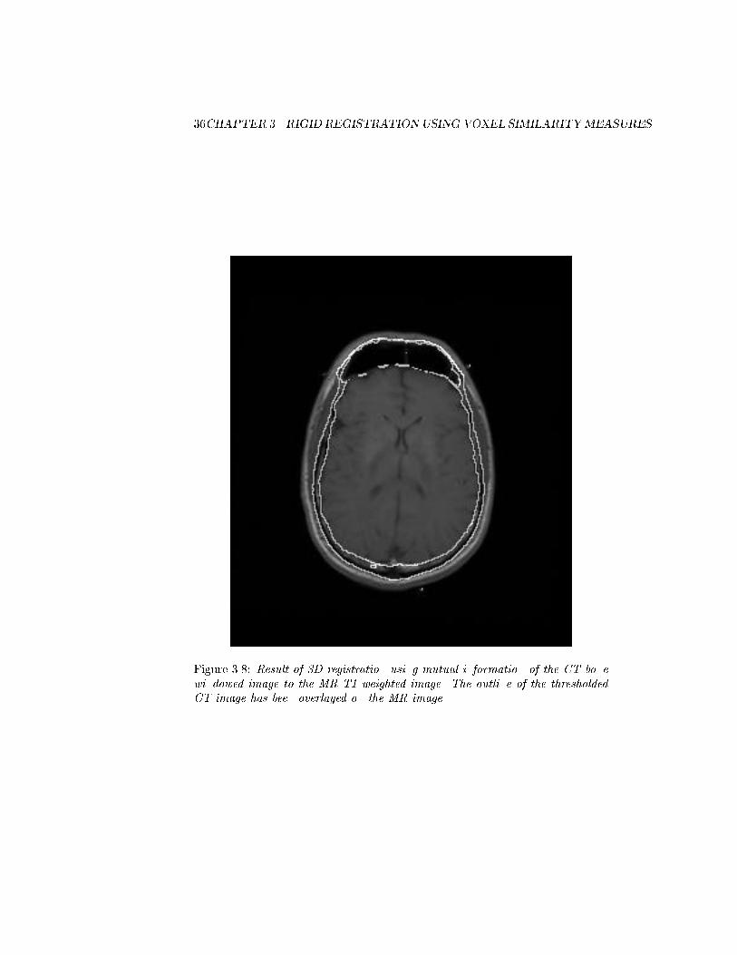
36CHAPTER 3. RIGID REGISTRATIONUSING VOXEL SIMILARITYMEASURES
Figure 3.8: Result of 3D registration using mutual information of the CT bonewindowed image to the MR T1 weighted image. The outline of the thresholdedCT image has been overlayed on the MR image.

3.4. SUMMARY 37
Figure 3.9: Result of 3D registration using mutual information of the CT bonewindowed image to the MR T1 weighted image. The outline of the thresholdedCT image has been overlayed on the MR image.
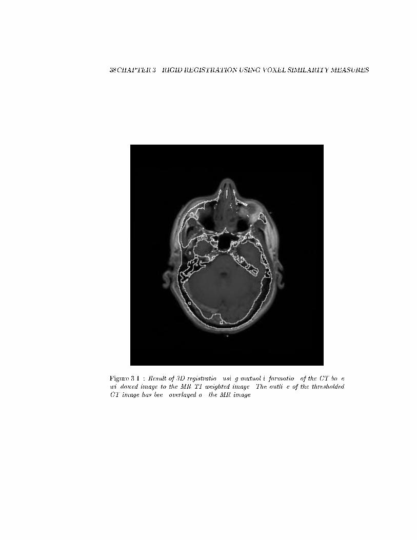
38CHAPTER 3. RIGID REGISTRATIONUSING VOXEL SIMILARITYMEASURES
Figure 3.10: Result of 3D registration using mutual information of the CT bonewindowed image to the MR T1 weighted image. The outline of the thresholdedCT image has been overlayed on the MR image.

3.4. SUMMARY 39
Figure 3.11: Result of 3D registration using mutual information of the CT bonewindowed image to the Red channel of the cryosection image. The outline ofthe thresholded CT image has been overlayed on the Red image.
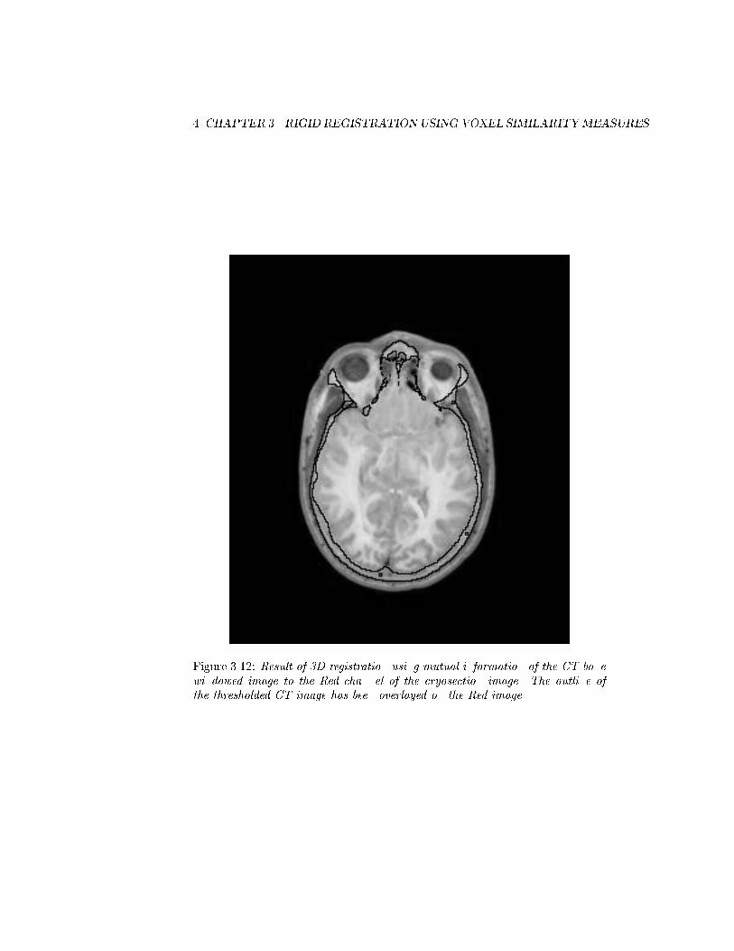
40CHAPTER 3. RIGID REGISTRATIONUSING VOXEL SIMILARITYMEASURES
Figure 3.12: Result of 3D registration using mutual information of the CT bonewindowed image to the Red channel of the cryosection image. The outline ofthe thresholded CT image has been overlayed on the Red image.
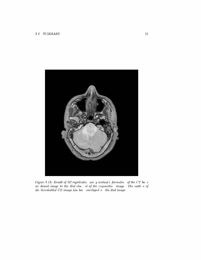
3.4. SUMMARY 41
Figure 3.13: Result of 3D registration using mutual information of the CT bonewindowed image to the Red channel of the cryosection image. The outline ofthe thresholded CT image has been overlayed on the Red image.

42CHAPTER 3. RIGID REGISTRATIONUSING VOXEL SIMILARITYMEASURES
Since most of the texture measures were dependent on the position in theGLCM, in contrast to the information theoretic measures, it should be ex-plored whether position dependent weights adapted to the registration problem(modality combination) could improve registration results. Preliminar work inthis direction did not yield positive results.
Chapter 4
Physical Continuum Models
Physical continuum models of elasticity etc. are well-known in computer visionand computer graphics, where they have been used for many years to track andmodel non-rigid shapes. Although they seldom have been actual models of thephysical phenomena and rather have been used to regularize problems, they haveenjoyed great succes.
Because of the emphasis on the regularization eect, these models have oftenbeen used without much understanding of their limitations and relationships.But, in recent years, and in particular in the core elds of this thesis - registrationand simulation - attention has begun to turn towards understanding rather thanblind use of the models.
In medical image registration, some of the rst work on non-rigid regis-tration used linear elastic models [Baj89, Chr94]. Christensen et al. illus-trated in [Chr94b, Chr94c] that for large deformations, the invalid assump-tion of linearity of the elasticity operator, can cause changes in the topologyof the images. Christensen et al. solved this problem by applying models of uids [Chr94b, Chr94c] or hyperelasticity (Rabbitt et al. [Rab95]) which canhandle large deformations.
This chapter presents a coherent description of the elastic and viscous uidcontinuum models of deformation used in the thesis. By using a consistentnotation, it is shown how elastic and uid transformations are closely related toeach other. The assumptions used in dierent practical models are described,and the relationship to previous work is shown.
4.1 Introduction
The continuum models, that are presented in this chapter, can all be describedby the sequential relationship between the four factors: Displacement, strain,stress and force (see gure 4.1). By displacement we understand the movementof particles in the continuum. This movement changes the conguration ofsmall volume element, and we measure this using strain tensors (in practice 3x3
43
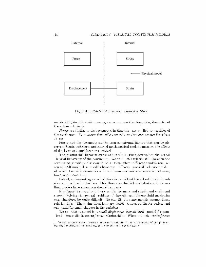
44 CHAPTER 4. PHYSICAL CONTINUUM MODELS
Physical model
InternalExternal
Stress
Strain
Force
Displacement
Figure 4.1: Relationship between physical entities.
matrices). Using the strain tensors, we can express the elongation, shear etc. ofthe volume elements.
Forces are similar to displacements, in that they are applied to particles ofthe continuum. To measure their eect on volume elements we use the stresstensor.
Forces and displacements can be seen as external factors that can be ob-served. Strain and stress are internal mathematical tools to measure the eectsof displacements and forces respectively.
The relationship between stress and strain is what determines the actualphysical behaviour of the continuum. We study this relationship closer in thesections on elastic and viscous uid motion, where dierent models are pre-sented. Although these models have very dierent practical behaviours, theyall satisfy the basic assumptions of continuum mechanics: conservation of mass,force, and momentum.
Indeed, an interesting aspect of this chapter is that the actual physical mod-els are introduced rather late. This illustrates the fact that elastic and viscous uid models have a common theoretical basis.
Non-linearities occur both between displacement and strain, and strain andstress1. Solving the general problems of elasticity and viscous uid mechanicscan, therefore, be quite dicult. To simplify it, some models assume linearrelationships. These simplications are basicly truncated Taylor series, andonly valid for small changes in the variables.
We say that a model is a small displacement/small strain model for com-pletely linear displacement/stress relationships. When only the strain/stress
1Forces are not always constant and can contribute to the non-linearity of the problem.For the simplicity of the presentation we ignore that in this chapter.
4.2. MATHEMATICAL PRELIMINARIES 45
relation is linear we say that the model is a large displacement/small strainmodel, etc.
4.2 Mathematical preliminaries
This section presents the mathematical conventions used in this and later chap-ters.
For sets, the plus operator is dened as working on non-overlapping sets andyielding the union of the sets:
A+B A [ B; A \ B = ; (4.1)
Vectors and matrices are written with bold letters. Lower case signiesvectors (eg. v) and upper case matrices (eg. M ). In general, the subelementsof vectors and matrices are denoted vi and Mij respectively. In addition, for
positions in space we use x = [x; y; z]T.
The zero vector and zero matrix are dened as o and 0 respectively.Let @f=@x be the partial derivative of the function f. We dene:
fxi = @if =@f
@xi(4.2)
The gradient operator r is dened as:
r =
@
@x;@
@y;@
@z
T(4.3)
Used with a scalar function f it yields the gradient vector of the function:
rf = [fx; fy; fz]T (4.4)
With vectors we override the r as:
ru (r(uT ))T
= [ux;uy;uz] =
24 @1u1 @2u1 @3u1
@1u2 @2u2 @3u2@1u3 @2u3 @3u3
35 (4.5)
The divergence of a vector is implemented using r as:
r u div u =rTu = @1u1 + @2u2 + @3u3 = tr(ru) (4.6)
and for matrices as:
r M divM = (rTM)T
=
24 @1M11 + @2M21 + @3M31
@1M12 + @2M22 + @3M32
@1M13 + @2M23 + @3M33
35 (4.7)
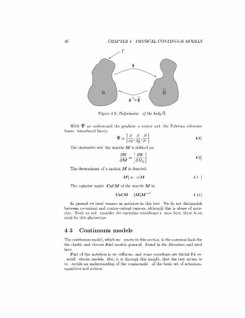
46 CHAPTER 4. PHYSICAL CONTINUUM MODELS
ϕ = ϕ
Γ
Ω
ϕ
−1 ∼Ω∼
Figure 4.2: Deformation of the body .
With ~r we understand the gradient operator wrt. the Eulerian referenceframe (introduced later):
~r =
@
@~x;@
@~y;@
@~z
(4.8)
The derivative wrt. the matrix M is dened as:
@W
@M=
@W
@Mij
(4.9)
The determinant of a matrix M is denoted:
jM j = detM (4.10)
The cofactor matrix CofM of the matrix M is:
CofM = jM jMT (4.11)
In general we treat tensors as matrices in this text. We do not distinquishbetween co-variant and contra-variant tensors, although this is abuse of nota-tion. Since we only consider the cartesian coordinate system here, there is noneed for this distinction.
4.3 Continuum models
The continuum model, which we present in this section, is the common basis forthe elastic and viscous uid models generally found in the literature and usedhere.
Part of the notation is super uous, and some equations are trivial for es-pecially elastic models. But, it is through this insight, that the text attemptsto provide an understanding of the commonality of the basic set of notations,equations and axioms.
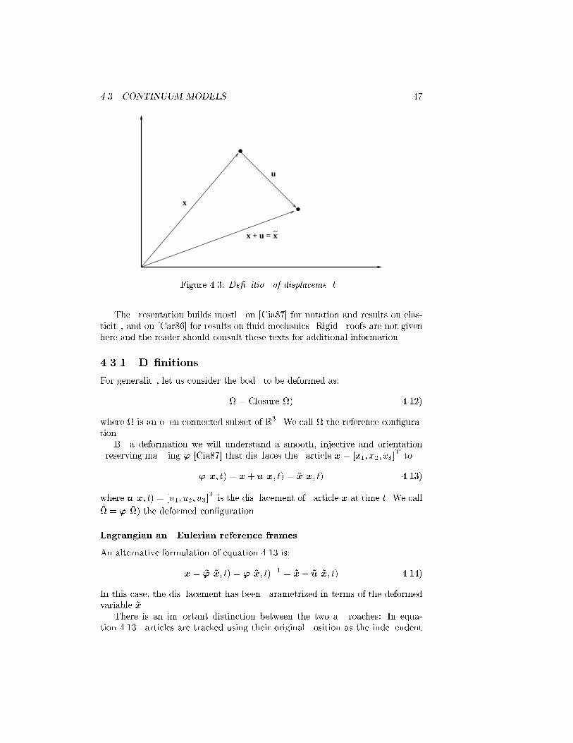
4.3. CONTINUUM MODELS 47
x~x + u =
u
x
Figure 4.3: Denition of displacement.
The presentation builds mostly on [Cia87] for notation and results on elas-ticity, and on [Car86] for results on uid mechanics. Rigid proofs are not givenhere and the reader should consult these texts for additional information.
4.3.1 Denitions
For generality, let us consider the body to be deformed as:
= Closure() (4.12)
where is an open connected subset of R3. We call the reference congura-tion.
By a deformation we will understand a smooth, injective and orientationpreserving mapping ' [Cia87] that displaces the particle x = [x1; x2; x3]
Tto
'(x; t) = x+ u(x; t) = ~x(x; t) (4.13)
where u(x; t) = [u1; u2; u3]Tis the displacement of particle x at time t. We call
~ = '() the deformed conguration.
Lagrangian and Eulerian reference frames
An alternative formulation of equation 4.13 is:
x = ~'(~x; t) = '(~x; t)1 = ~x ~u(~x; t) (4.14)
In this case, the displacement has been parametrized in terms of the deformedvariable ~x.
There is an important distinction between the two approaches: In equa-tion 4.13 particles are tracked using their original position as the independent
48 CHAPTER 4. PHYSICAL CONTINUUM MODELS
variable. This parametrization is mostly used in elasticity and is called theLagrangian reference frame. In uid mechanics, tracking particles using theiroriginal position x can be cumbersome for very large deformations. Instead thecurrent position ~x is used as in equation 4.14. This parametrization is calledthe Eulerian reference frame. We use a tilde (~) to denote entities parametrizedusing this reference frame. A particle ~x in the Eulerian reference frame at timet, originated from position x = ~'(~x; t) at time t0.
Note, that displacements and velocities are physical entities and independentof the reference frame:
u(x; t) = ~u(~x; t)
v(x; t) = ~v(~x; t) (4.15)
In the Lagrangian reference frame the velocities are calculated directly using:
v(x; t) =@'(x; t)
@t
=
@~x(x; t)
@t
=
@u(x; t)
@t(4.16)
But, in the Eulerian reference frame the coordinate system depends on the timevariable, and a full derivative has to be used:
~v(~x; t) =d
dt~u(~x; t) (4.17)
With the chain rule we nd:
d
dt~u(~x; t) =
@~u
@t
(~x;t)
+Xi
@~u
@~xi
(~x;t)
@~xi@t
(x;t)
(4.18)
Using equation 4.16 we write this as:
d
dt~u(~x; t) =
@~u
@t
(~x;t)
+ ~r~u(~x; t) ~v(~x; t) (4.19)
which is called the material derivative of ~u in the Eulerian reference frame.Let us now consider the integral:
f =
Z~(t)
g d~x (4.20)
for the arbitrary function g. We take the material derivative of this integral:
df
dt=
d
dt
Z~g d~x (4.21)
and transform it to the reference conguration (d~x = jr'(x)jdx):d
dt
Z~g d~x =
d
dt
Z(gjr'(x)j) dx (4.22)
4.3. CONTINUUM MODELS 49
In this case, since the volume of integration is independent of the time variablet, the derivative can be brought inside the integration sign.
d
dt
Z~g d~x =
Z
d
dt(gjr'(x)j) dx (4.23)
Using the result that @jr'(x)j=@t = (r v)jr'(x)j [Car86] and transformingback to the deformed conguration:
d
dt
Z~g d~x =
Z~
dg
dt+ g ~r ~v
d~x (4.24)
Or using the material derivative equation:
d
dt
Z~g d~x =
Z~
@g
@t+ ~r (g~v)
d~x (4.25)
This is the formal statement of the transport theorem.The material derivative and the transport theorem describe how simple vari-
ables and integrals can be dierentiated wrt. time in the Eulerian referenceframe.
4.3.2 Strain
To measure the local deformation we introduce the deformation gradient:
r' ='x;'y;'z
=
24 @1'1 @2'1 @3'1
@1'2 @2'2 @3'2@1'3 @2'3 @3'3
35 (4.26)
Since the deformation is orientation preserving by denition, the determinantof the deformation should satisfy the condition:
jr'(x; t)j > 0; 8x 2 (4.27)
jr'(x; t)j is the Jacobian of the transformation and commonly denoted J inthe literature.
We also express the deformation gradient in terms of the displacement gra-dient ru:
r' = I +ru (4.28)
Using the deformation gradient, we dene the right Cauchy-Green straintensor2:
C =r'Tr' (4.29)
C is symmetric and positive denite because r' is invertible (jr'j > 0).The strain tensor is supposed to be a measure of the pure deformation of
the domain, and independent of rigid transformations. To investigate whether
2In dierential geometry, this is also known as the metric tensor

50 CHAPTER 4. PHYSICAL CONTINUUM MODELS
this is the case, we assume that the deformation ' can be split into a non-rigid(ud) and rigid (R; t) part:
'(x) = R(x+ ud) + t; R 2 Q3 (4.30)
where Q3 is the set of rotation matrices, ie. orthonormal matrices of size 3 withdeterminant +1. The deformation gradient becomes:
r'(x) = Rr(x+ ud) = R(I +rud) = Rr'd(x) (4.31)
Which also follows from the polar factorization theorem ([Cia87], theorem 3.2-2).
We can now calculate the strain tensor C:
C = r'(x)Tr'(x) = (Rr'd(x))TRr'd(x)
= r'd(x)TRTRr'd(x)
= r'd(x)Tr'd(x) = Cd (4.32)
Thus the strain tensor C is independent of the rigid component. For completelyrigid motion the strain tensor is the identity matrix, C = I .
Another well-known strain tensor is the Green-St. Venant strain tensor3:
E =1
2(C I) =ruT +ru+ruTru (4.33)
The subtraction of I ensures that this tensor is zero for rigid transformations,and it can, therefore, be seen as a measure of the pure deformation. The factor12 has been introduced for historical reasons.
In general, a number of dierent strain tensors exist. There is no 'best'strain tensor, and they can all be derived from each other.
The velocity can be analyzed in a similar fashion. The spatial velocity gra-dient is dened as:
L(x;') =rv(x) (4.34)
The symmetric part of L is called the rate of strain tensor:
D =1
2(L+LT ) (4.35)
4.3.3 Forces
We assume that in the deformed conguration ~ with the boundary ~ = @ ~,two kinds of forces are applied to the body:
Applied body forces which work on the interior of the body:
~f : ~! R3 (4.36)
where ~f is the density of the applied body force per unit volume in thedeformed conguration.
3Also known as the Almansi or Green-Lagrange strain tensor
4.3. CONTINUUM MODELS 51
Applied surface forces which work on the boundary of the domain:
~g : ~1 ! R3 (4.37)
where ~g is the density of the applied surface forces per unit surface areain the deformed conguration, and ~1 is a subset of the full boundary~ = ~0 + ~1. Fixed displacements are applied to the other part of theboundary (~0).
We note that these forces are given in the Eulerian reference frame. Sincef(x)dx = ~f(~x)d~x and d~x = jr'(x)jdx using the Jacobian, we have that:
f(x) = jr'(x)j ~f(~x) (4.38)
A similar relation exists for the surface forces [Cia87]:
g(x) = jr'(x)j kr'(x)Tnk ~g(~x) (4.39)
and the mass density(x) = jr'(x)j ~(~x) (4.40)
4.3.4 Equations of motion for a continuum
The elastic and viscous uid continuum models all satisfy the basic physicalaxioms of balance of mass, and linear and angular momentum. We discussthese axioms and their implications in general terms in this section. The nextsection will introduce model specic considerations.
Conservation of mass
The axiom of conservation of mass, means that the total mass of the body isconstant. Constant mass also implies that for an arbitrary volume ~V ~ wecan write:
d
dt
Z~V
~(~x; t) d~x = 0 (4.41)
where ~ is the density in the deformed conguration.Setting g = ~ in the transport theorem (4.25) we get:Z
~V
@~
@t+ ~r (~~v)
d~x = 0 (4.42)
Since the volume ~V is an arbitrary subset of the domain, we can extract theintegrand as the continuity equation:
@~
@t+ ~r (~~v) = 0 (4.43)
For incompressible continua, ~ is constant, and:
~r ~v = 0 (4.44)

52 CHAPTER 4. PHYSICAL CONTINUUM MODELS
Stress tensor - conservation of momentum
In this section we consider a small volume element. From the axioms of localbalance of linear momentum and balance of angular moment it follows accordingto the Cauchy theorem [Cia87], that for each volume element of the body, thereexists a vector eld ~t(~x; ~n) and a symmetric tensor eld ~T (~x), such that:
~t(~x; ~n) = ~T (~x)~n (4.45)
where ~n is the unit outer normal to the surface of the volume element. ~t and~T are called the Cauchy stress vector and Cauchy stress tensor respectively. Atthe boundary of the domain ~t(~x; ~n) = ~g(~x).
The axiom of global conservation of linear momentum can be written for anarbitrary subset ~V ~ as:
d
dt
Z~V
~~vd~x =
Z~V
~f (~x)d~x+
Z@ ~V
~t(~x; ~n)d~a (4.46)
where ~f is the force working on a volume element in the interior of the body.Using Gauss's divergence theorem, the transport theorem and the continuityequation, we rewrite this as:Z
~V
~
@~v
@t+ ( ~r~v)~v
d~x =
Z~V
~f(~x)d~x+
Z~V
~r ~T (~x)d~x (4.47)
After collecting terms and using the material derivative equation:Z~V
~d~v
dt ~f(~x) ~r ~T (~x)
d~x = 0 (4.48)
Since this has to hold for any sub-volume of the continuum, the integrand mustbe independently zero and we nd the momentum equation:
~d~v
dt= ~f(~x) + ~r ~T (4.49)
Summary
In this section we have derived the general equations of motion for a continuum:
~d~v
dt= ~f(~x) +r ~T (~x); ~x 2 ~ (4.50)
~g(~x) = ~T (~x)~n; ~x 2 ~ (4.51)
Together with the formulas for displacement, velocity and strain these equationsform a general set of equations for continuum models. In the next section specicmodels will be introduced linking stress to strain. This linkage is what denesthe actual physical characteristics of the continuum.
4.4. ELASTIC CONTINUUM MODELS 53
We note that equations 4.50-4.51 have similar formulations in the Lagrangianreference frame. We associate with ~T the non-symmetric rst Piola-Kirchostress tensor T :
T (x) = jr'(x)j ~T (~x)(r'(x))T = ~T (~x)Cof'(x) (4.52)
The main advantage of this choice is the simple relationship between the diver-gences of both tensors:
r T (x) = jr'(x)j ~r ~T (~x) (4.53)
thus giving equation 4.50 in the Lagrangian reference frame as:jr'(x)j~d~v
dt=
d2u
dt2= f(x) +r T (x) (4.54)
One can also transform the Cauchy stress vector ~t into a vector in such a waythat:
t(x;n) = T (x)n (4.55)
where n is the normal vector of the undeformed subdomain. It follows, usingequation 4.39, that t(x;n) = g(x) on 1 and we can write equation 4.51 in theLagrangian reference frame as:
g(x) = T (x)n; x 2 1 (4.56)
In some cases a symmetric stress tensor is desirable. We, therefore, dene thesecond Piola-Kirchho stress tensor by:
(x) =r'(x)1T (x) (4.57)
For elastic motion, equation 4.54 corresponds to harmonic motion. A damp-ing factor cdu
dtis often added to give the equation for damped harmonic motion4:
d2u
dt2+ c
du
dt= f(x) +r T (x) (4.58)
For static elastic deformation, the motion equation is rewritten as:
o = f (x) +r T (x) (4.59)
The time derivatives are all zero because there is no temporal change.
4.4 Elastic continuum models
An elastic material is characterized by a deterministic relationship betweenstress and strain which is independent of any history.
4The equation for damped harmonic motion is often called the Lagrangian equation ofmotion
54 CHAPTER 4. PHYSICAL CONTINUUM MODELS
The stress/strain relationship of a general class of elastic materials can bedescribed using the concept of stored energy. These materials are called hyper-elastic materials, and the stored energy function W completely determines thestress/strain relation by:
(x;') =r'(x)1T (x) =@W
@E(x;') (4.60)
where E is the Green-St. Venant strain tensor (4.33).Although these hyperelastic materials do not cover all elastic material mod-
els, they form a general class of materials which covers most practical materialmodels.
The potential strain energy for the body can be written using the storedenergy function as:
Estrain(') =
ZW(x;')dx (4.61)
For isotropic and homogeneous materials the stored energy function is com-pletely characterized by the socalled principal invariants of the right Cauchy-Green strain tensor C. These invariants appear as the coecients in the charac-teristic polynomial jCI j, and are written in terms of the right Cauchy-Greenand Green-St. Venant strain tensors as:
1 = trC = 3 + 2trE
2 = 12 [(trC)2=trC2] = 3 + 4trE + 2[(trE)2 trE2]
3 = jCj = j2E + I j(4.62)
Using these invariants the stored energy function for the general hyperelasticmaterial can be formulated as an innite series:
W =1X
rst=0
Crst(1 3)r(2 3)s(3 1)t; C000 = 0 (4.63)
It is interesting to note, that the third invariant measures the volume changeof an innitesimal volume element. For incompressible materials this invariantmust be trivially 1. An often used approach to enforce the incompressibilityconstraint, is to introduce a Lagrange multiplier which then works as aninternal pressure, forcing the material to nd an incompressed equilibrium state.The incompressible version of the stored energy can be written as:
Wi =
1Xrs=0
Cirs(1 3)r(2 3)s + (3 1); Ci
00 = 0 (4.64)
In the next sections the Mooney-Rivlin and St. Venant Kirchho material mod-els are introduced. TheMooney-Rivlin material model is a completely non-linearmodel in both the stress/strain and the displacement/strain relationships. TheSt. Venant Kirchho material model is linear in the stress/strain relationship,but non-linear in strain/displacement. Because it is the simplest of the non-linear hyperelastic material models, it is often used. More popular, though, is
4.4. ELASTIC CONTINUUM MODELS 55
the linearized version, where the strain/displacement relationship is made linearby the assumption of innitesimal displacements. This linearized version of theSt. Venant Kirchho model is also known as linear elasticity or Hooke's Law.
4.4.1 Mooney-Rivlin materials
The compressible Mooney-Rivlin material model is described by the approxima-tion to the general stored energy function by:
W = C100(1 3) + C010(2 3) + (pj3j) (4.65)
() = c2 d log ; c; d > 0
The -function ensures that large volume changes are accompanied by innitestress.
The incompressible version ignores the third element and can be written as:
W = C100(1 3) + C010(2 3); j3j = 1 (4.66)
The Mooney-Rivlin material model has been used in surgery simulation andfor general modeling of human tissue, eg. [Sag94, Beg88].
4.4.2 St. Venant Kirchho materials
For Crst = 0 except for
C100 = C200 =+ 2
8C010 =
3(4.67)
we get the St. Venant Kirchho material model:
W =
2(trE)2 + trE2 (4.68)
where and are the Lame material constants.Note, that this material model has a linear stress/strain relationship, since:
=@W
@E= (trE)I + 2E (4.69)
and that the volume change measured by 3 does not play any role.The St. Venant Kirchho material has been used in computer graphics (eg.
Terzopoulos [Ter88]).
4.4.3 Linear elastic materials
Linear elasticity is with no doubt the most well-known of the elastic models.It has the remarkable property, that it is completely linear in terms of theforce/displacement relationship. Systems derived from the linear elastic op-erator are, consequently, easy to solve compared to the other elastic models

56 CHAPTER 4. PHYSICAL CONTINUUM MODELS
which in general are non-linear. Unfortunately, the assumption leading to thelinerization of the St. Venant Kirchho material model is seldom satised.
The basic assumption is that the non-linear Green-St. Venant strain tensor:
E =1
2(C I) = 1
2[ruT +ru+ruTru] (4.70)
can be approximated by the linearized strain tensor
El =1
2[ruT +ru] (4.71)
This is only valid for innitesimal displacements, since in that case the quadraticterm ruTru disappears.
Using the linearized Green-St. Venant strain tensor we can write the storedenergy function for the linear approximation of the St. Venant Kirchho materialmodel as:
Wl =
2(trEl)
2 + trE2l (4.72)
The linear elastic material model is popularly known as Hooke's Law.To follow the "engineering" notation often used with linear elasticity, we
introduce the engineering strain vector :
= [ux; vy; wz ; uy + vx; uz + wx; vz + wy]T (4.73)
The linearized strain tensor can be written as:
El =1
2[ruT +ru]
=
24 ux
12 [uy + vx]
12 [uz + wx]
12 [uy + vx] vy
12 [vz + wy ]
12 [uz + wx]
12 [vz + wy] wz
35 (4.74)
We note that:
trEl = [111000] = ht
trE2l = TDiag
111
1
2
1
2
1
2
= TH (4.75)
We can thus rewrite the linearized St. Venant Kirchho stored energy functionas:
Wl =
2(trEl)
2 + trE2l
=
2(hT )2 + TH
=1
2T [hhT + H]
=1
2TM =
1
2T (4.76)
4.5. VISCOUS FLUID CONTINUUM MODELS 57
where =M is the engineering stress vector and M is the material matrix:
M = hhT + H =
26666664
+ 2 0 0 0 + 2 0 0 0 + 2 0 0 00 0 0 0 00 0 0 0 00 0 0 0 0
37777775
(4.77)
To those familiar with linear elasticity, the stored energy function might be morerecognizable, when written using the actual partial derivatives:
Wl =
3Xi=1
3Xj=1
2(@iui) (@juj) +
4(@jui + @iuj)
2(4.78)
The governing partial dierential equation (PDE) for static linear elastic defor-mation is formulated using equation 4.69:
o = f (x) +r T (x) (4.79)
= f (x) + u(x) + (+ )r(r u(x))
where =rTr is the Laplacian operator.
The linear elastic material model has been used in both computer graphics(eg. [Gou89, Pie92, BN96c]), and image processing (eg. [Baj89, Mil93]).
Two other well-known linear material models are the Laplacian or membranemodel:
Wlmembrane =
Xi=1
(@iui)2
(4.80)
0 = f (x) +u(x)
and the biharmonic or thin-plate model:
Wlthinplate =
Xi=1
Xj=1
@2ijui
2(4.81)
0 = f(x) +2u(x)
The membrane model can be seen as a simplication of the linear elastic model,where the cross-directional eects due to r(r u(x)) are ignored.
These models have been used extensively in image processing and computervision, both alone (eg. [Boo89]) and together (eg. [Kas88, Coh89]).
4.5 Viscous uid continuum models
In contrast to elastic models the strain in uid models is history dependent.Elastic models are characterized by spatial smoothing of the displacement eld.
58 CHAPTER 4. PHYSICAL CONTINUUM MODELS
Fluid models, on the other hand, are characterized by spatial smoothing of thevelocity eld. In practice, this means that any displacement can be obtainedgiven enough time because the internal stresses in the uid disappear temporar-ily.
The uid model used in this thesis is dened by the viscous uid Navier-Stokes equations, which we derive below.
As a rst step, the viscous and pressure contributions to the stress tensorare written explicitly:
~T = ~V ~pI (4.82)
where ~V is the reduced stress tensor representing the viscous eects, and ~p isthe pressure.
The basic assumption of the Navier-Stokes equations is based on Stokes'hypothesis. This hypothesis states that ~V is a function of the deformation rate
tensor ~D = 12 (~L + ~L
T) which is the symmetric part of the spatial velocity
gradient ~L (equation 4.34). The relation is:
~V = 2 ~D + ( ~r ~v)I (4.83)
Inserting this into the momentum equation gives:
~d~v
dt= ~f ~r~p+ ~~v + (+ ) ~r( ~r ~v) (4.84)
where ~ = ~rT ~r is the Laplacian5.
For very low Reynold's number 6 ow, a simplied model is obtained when
we ignore the pressure gradient ~r~p and the inertial term ~d~vdt
[Chr94c]:
o = ~f + ~~v + (+ ) ~r( ~r ~v) (4.85)
Surprisingly, this is actually the linear elasticity PDE (equation 4.80), wherethe displacement u has been replaced by the velocity ~v. This similarity is usedextensively to transfer results from linear elasticity to the solution of the viscous uid problem.
4.6 Eigen-function parametrization of the linearelastic operator
In this section we focus on the linear operator associated with linear elasticity:
Lu = u(x) + (+ )r(r u(x)) (4.86)
Following the approach of Miller, Christensen, et al. [Chr94, Chr94c, Mil93], wereparametrize the linear elasticity operator using the eigen-functions and eigen-values for a specic case of boundary conditions. Since mapping the boundary
5The and parameters are not the same as those used for linear elastic transformations.We use the same notation anyway for simplicity
6The Reynold's number is a measure of the 'velocity' or complexity of the uid motion.
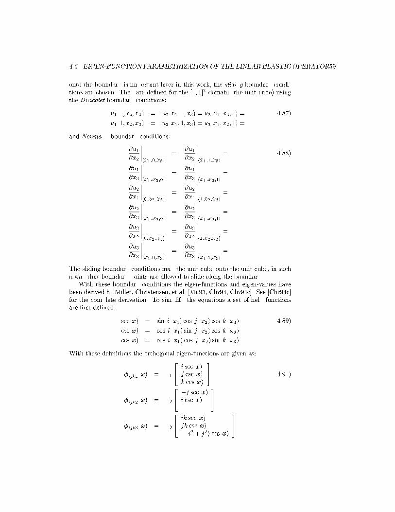
4.6. EIGEN-FUNCTION PARAMETRIZATIONOF THE LINEAR ELASTIC OPERATOR59
onto the boundary is important later in this work, the sliding boundary condi-tions are chosen. They are dened for the [0; 1]3 domain (the unit cube) usingthe Dirichlet boundary conditions:
u1(0; x2; x3) = u2(x1; 0; x3) = u3(x1; x2; 0) = 0 (4.87)
u1(1; x2; x3) = u2(x1; 1; x3) = u3(x1; x2; 1) = 0
and Neumann boundary conditions:
@u1@x2
(x1;0;x3)
=@u1@x2
(x1;1;x3)
= 0 (4.88)
@u1@x3
(x1;x2;0)
=@u1@x3
(x1;x2;1)
= 0
@u2@x1
(0;x2;x3)
=@u2@x1
(1;x2;x3)
= 0
@u2@x3
(x1;x2;0)
=@u2@x3
(x1;x2;1)
= 0
@u3@x2
(0;x2;x3)
=@u3@x2
(1;x2;x3)
= 0
@u3@x3
(x1;0;x3)
=@u3@x3
(x1;1;x3)
= 0
The sliding boundary conditions map the unit cube onto the unit cube, in sucha way that boundary points are allowed to slide along the boundary.
With these boundary conditions the eigen-functions and eigen-values havebeen derived by Miller, Christensen, et al. [Mil93, Chr94, Chr94c]. See [Chr94c]for the complete derivation. To simplify the equations a set of help functionsare rst dened:
scc(x) = sin(ix1) cos(jx2) cos(kx3) (4.89)
csc(x) = cos(ix1) sin(jx2) cos(kx3)
ccs(x) = cos(ix1) cos(jx2) sin(kx3)
With these denitions the orthogonal eigen-functions are given as:
ijk1(x) = 1
24 i scc(x)
j csc(x)k ccs(x)
35 (4.90)
ijk2(x) = 2
24 j scc(x)
i csc(x)0
35
ijk3(x) = 3
24 ik scc(x)
jk csc(x)(i2 + j2) ccs(x)
35
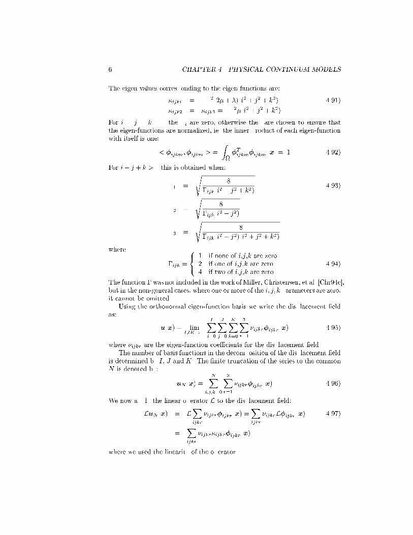
60 CHAPTER 4. PHYSICAL CONTINUUM MODELS
The eigen-values corresponding to the eigen-functions are:
ijk1 = 2(2+ )(i2 + j2 + k2) (4.91)
ijk2 = ijk3 = 2(i2 + j2 + k2)
For i = j = k = 0 the i are zero, otherwise they are chosen to ensure thatthe eigen-functions are normalized, ie. the inner product of each eigen-functionwith itself is one:
< ijkm;ijkm > =
ZTijkmijkmdx = 1 (4.92)
For i+ j + k > 0 this is obtained when:
1 =
s8
ijk(i2 + j2 + k2)(4.93)
2 =
s8
ijk(i2 + j2)
3 =
s8
ijk(i2 + j2)(i2 + j2 + k2)
where
ijk =
8<:
1 if none of i,j,k are zero2 if one of i,j,k are zero4 if two of i,j,k are zero
(4.94)
The function was not included in the work of Miller, Christensen, et al. [Chr94c],but in the non-general cases, where one or more of the i; j; k parameters are zero,it cannot be omitted.
Using the orthonormal eigen-function basis we write the displacement eldas:
u(x) = limIJK!1
IXi=0
JXj=0
KXk=0
3Xr=1
ijkrijkr(x) (4.95)
where ijkr are the eigen-function coecients for the displacement eld.The number of basis functions in the decomposition of the displacement eld
is determined by I , J and K. The nite truncation of the series to the commonN is denoted by:
uN (x) =
NXi;j;k=0
3Xr=1
ijkrijkr(x) (4.96)
We now apply the linear operator L to the displacement eld:
LuN (x) = LXijkr
ijkrijkr(x) =Xijkr
ijkrLijkr(x) (4.97)
=Xijkr
ijkrijkrijkr(x)
where we used the linearity of the operator.
4.6. EIGEN-FUNCTION PARAMETRIZATIONOF THE LINEAR ELASTIC OPERATOR61
4.6.1 Projection of forces onto the eigen-function basis
Let us consider the static elastic deformation equation using linear elasticity:
Lu(x) + f(x) = o (4.98)
where f is the applied force eld. Using the truncated decomposition in equa-tion 4.97 we rewrite this as:X
ijkr
ijkrijkrijkr(x) + f(x) = o (4.99)
We take the inner product < a; b >=RaT bdx of the equation with lmns(x)
and get: Xijkr
ijkrijkr < ijkr(x);lmns(x) > + < f(x);lmns(x) > = o
mlmnslmns+ < f (x);lmns(x) > = o
mlmns = 1
lmns
< f (x);lmns(x) > (4.100)
where the fact, that < ijkr(x);lmns(x) > is zero for (ijkr) 6= (lmns), wasused to pick out the lmns element of the summation, in the step from line 1 toline 2. We call equation 4.100 the decomposition projection equation.
This result is interesting, since it provides us with a simple way of deter-mining the coecients for the eigen-function decomposition of the displacementeld given a force f . Indeed the eigen-basis coecients are simply the projec-tion by the inner product of the force onto the eigen-functions, scaled by theinverse of the eigen-values.
4.6.2 2D eigen-function basis
For completeness we also give the eigen-functions and eigen-values for the 2Dversion of the linear elastic operator:
Lu = u(x) + (+ )r(r u(x)) (4.101)
With the sliding boundary conditions on the domain [0; 1]2:
u1(0; x2) = u2(x1; 0) = 0 (4.102)
u1(1; x2) = u2(x1; 1) = 0
@u1@x2
(x1;0)
=@u1@x2
(x1;1)
= 0 (4.103)
@u2@x1
(0;x2)
=@u2@x1
(1;x2)
= 0
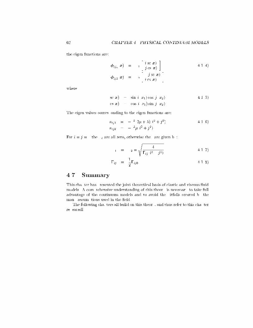
62 CHAPTER 4. PHYSICAL CONTINUUM MODELS
the eigen-functions are:
ij1(x) = 1
i sc(x)j cs(x)
(4.104)
ij2(x) = 2
j sc(x)i cs(x)
where
sc(x) = sin(ix1) cos(jx2) (4.105)
cs(x) = cos(ix1) sin(jx2)
The eigen-values corresponding to the eigen-functions are:
ij1 = 2(2+ )(i2 + j2) (4.106)
ij2 = 2(i2 + j2)
For i = j = 0 the i are all zero, otherwise they are given by:
1 = 2 =
s4
ij(i2 + j2)(4.107)
ij =1
2ij0 (4.108)
4.7 Summary
This chapter has presented the joint theoretical basis of elastic and viscous uidmodels. A comprehensive understanding of this theory is necessary to take fulladvantage of the continuum models and to avoid the pitfalls created by themany assumptions used in the eld.
The following chapters all build on this theory, and thus refer to this chapterrepeatedly.
Chapter 5
Non-rigid Registration
using Continuum Models
The subject of this chapter is non-rigid registration using physical continuummodels. The rst section denes the non-rigid registration problem. In thesecond section elastic registration methods are discussed.
Some of these methods use linear models of elastic deformation. Unfortu-nately, registration using linear elasticity often violates the inherent small defor-mation assumption. For large deformations the topology cannot be guaranteedand an alternative approach is needed.
The next section describes such an alternative registration method using vis-cous uid continuum models, which were originally proposed by Christensen etal. [Chr93, Chr94b, Chr94c, Chr96]. These models have the advantage that theyallow large complex deformations and implement free registration as opposedto elastic registration.
The chapter then proceeds to propose a new algorithm for viscous uidregistration, which is at least an order of magnitude faster than the previousalgorithm by Christensen et al. This speedup is important, since it allows theviscous uid registration algorithm to be run on an ordinary single-processorworkstation, instead of the massively parallel computer needed by the algorithmof Christensen et al.
The algorithm uses convolution with a new lter which implements the linearelasticity operator described in the previous chapter.
Thirion [Thi96] has recently proposed a 'demon'-based algorithm for freeregistration of medical images. We show that the work of Thirion is actuallya primitive version of the uid registration algorithm, and discuss the possibleconsequences of the use of the Gaussian lter in Thirion's work, instead of ourlinear elasticity lter. The advantage of the Gaussian lter is that it is separableand thus allows fast computation.
63

64CHAPTER 5. NON-RIGID REGISTRATIONUSING CONTINUUMMODELS
5.1 Dening the problem
Following the denitions of Christensen et al. [Chr93, Chr94b, Chr94c, Chr96]the non-rigid registration problem is regarded as a question of mapping or warp-ing a template image onto an individual study image.
The template image can be part of an anatomical atlas1, which possibly inaddition to the template image includes other modalities, topological informa-tion, functional information, etc.
Denote the template image T (x) and the study image S(x) where x 2 [0; 1]3.Formulated in the Lagrangian reference frame the purpose of the registration isconsequently to nd a transformation '(x) = x + u(x) that maps T (x) ontoS(x), in such a way that T (x) matches S('(x)). In the Eulerian reference framewe seek a transformation ~'(~x) = ~x ~u(~x) so that T (~'(~x)) matches S(~x).
The transformation '(x) : ! ~ must be homeomorphic to ensure thatthe transformation maintains the topology and structure of the original tem-plate image. A homeomorphic mapping is dened as being continuous, 1-to-1and onto. A thorough discussion of the homeomorphism can be found in Chris-tensen [Chr94c].
In practice, to ensure that the transformation is homeomorphic, we demandthat the boundary of the domain is mapped onto itself, and that the Jacobian ofthe transformation is greater than zero everywhere. The boundary requirementis satised, when xed or sliding boundary conditions are employed, as they arewith the linear elastic eigen-basis introduced in the section 4.6. Also note thatthe concatenation of homeomorphic mappings yields a homeomorphic mapping.
5.2 Elastic registration
Bajcsy et al. [Baj89, Gee93] were the rst to describe 3D voxel-based non-rigidregistration of medical images using elastic models. Building on initial work byBroit [Brt81], they modelled the template image as a linear elastic solid anddeformed it using forces derived from an approximation of the local gradient ofa correlation based similarity measure. In addition they used multi-resolutionto increase the speed.
Miller, Christensen, et al. [Mil93, Chr94] also used the linear elastic defor-mation model, but applied a Gaussian sensor model, ie. a least-squares measureof the grey-level dierences in the two images. To regularize the registrationproblem they rst registered the images using a truncated linear elastic eigen-basis (as dened in section 4.6), and then followed this initial registration witha registration using the full linear elastic model.
Christensen et al. [Chr94c] later realized, that using the linear elastic con-tinuum model was not appropriate, since the assumption of innitisimal defor-mation was frequently violated for the kind of deformation that is required innon-rigid registration. The transformation is not guaranteed to be homeomor-phic and, therefore, not well-behaved.
1Called anatomical textbook in Christensen et al. [Chr93, Chr94b, Chr94c, Chr96]
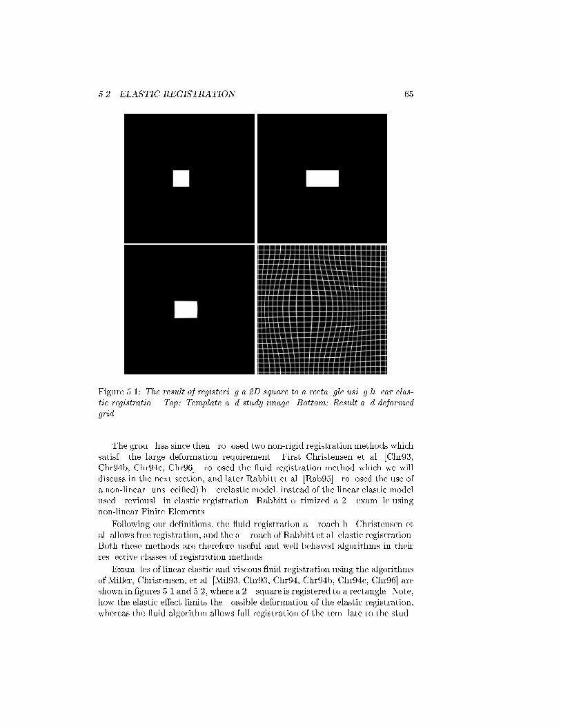
5.2. ELASTIC REGISTRATION 65
Figure 5.1: The result of registering a 2D square to a rectangle using linear elas-tic registration. Top: Template and study image. Bottom: Result and deformedgrid.
The group has since then proposed two non-rigid registration methods whichsatisfy the large deformation requirement. First Christensen et al. [Chr93,Chr94b, Chr94c, Chr96] proposed the uid registration method which we willdiscuss in the next section, and later Rabbitt et al. [Rab95] proposed the use ofa non-linear (unspecied) hyperelastic model, instead of the linear elastic modelused previously in elastic registration. Rabbitt optimized a 2D example usingnon-linear Finite Elements.
Following our denitions, the uid registration approach by Christensen etal. allows free registration, and the approach of Rabbitt et al. elastic registration.Both these methods are therefore useful and well-behaved algorithms in theirrespective classes of registration methods.
Examples of linear elastic and viscous uid registration using the algorithmsof Miller, Christensen, et al. [Mil93, Chr93, Chr94, Chr94b, Chr94c, Chr96] areshown in gures 5.1 and 5.2, where a 2D square is registered to a rectangle. Note,how the elastic eect limits the possible deformation of the elastic registration,whereas the uid algorithm allows full registration of the template to the study
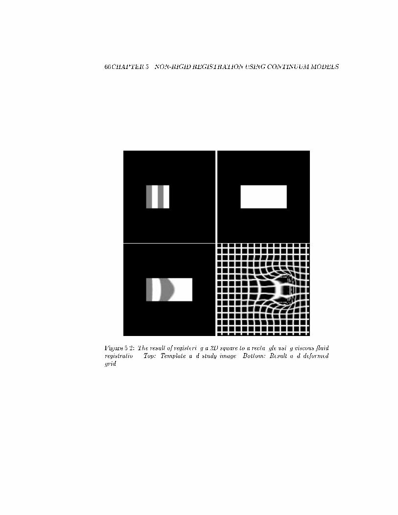
66CHAPTER 5. NON-RIGID REGISTRATIONUSING CONTINUUMMODELS
Figure 5.2: The result of registering a 2D square to a rectangle using viscous uidregistration. Top: Template and study image. Bottom: Result and deformedgrid.
5.3. VISCOUS FLUID REGISTRATION 67
image. This was also illustrated in gure 2.1 in chapter 2.The next section describes the viscous uid registration algorithm used by
Christensen et al. and then continues to propose a new and faster algorithm.
5.3 Viscous uid registration
In [Chr93, Chr94b, Chr94c, Chr96] Christensen et al. described a free regis-tration approach in which they use a viscous uid model to control the defor-mation. The template image is modelled as a thick uid which ows out tomatch the study, under the control of the same Gaussian sensor model usedin [Chr94, Mil93]. In [Chr94c] Christensen argues that this Gaussian sensormodel is theoretically better than correlation based similarity measures.
Unfortunately, the algorithm proposed by Christensen et al. is rather slow.They originally implemented the algorithm using a massively parallelDECmpp 128x64 MasPar computer, on which the algorithm used on the or-der of 5-10 minutes for 2D and 2-6 hours for 3D registrations. In a recentpaper [Chr96] they show estimates of the execution time on a MIPS R4400processor on the order of 2 hours for 2D and 7 days for 3D. In practice thismeans that the algorithm is not useful unless a massively parallel computer isavailable.
The contribution of this chapter is a new fast algorithm based entirely onconvolution with lters, which gives a speedup of at least an order of magnitude.
The original viscous uid algorithm by Christensen et al. [Chr93, Chr94b,Chr94c, Chr96] is rst described. The viscous uid model is introduced alongwith the force eld and the numerical solution method. We discuss the core partof Christensen's numerical solution, and introduce the general idea behind theconvolution approach, which is proposed to increase the speed of the method.And nally, the new lter for the convolution approach is derived.
5.3.1 Viscous uid model
Following Christensen et al., the viscous uid PDE dened in equation 4.85 isused. Note, that the viscous uid PDE was derived here without introducing themass source term that Christensen et al. use. Although, they emphasize theintroduction of this mass source term they quickly proceed to remove it, usingthe assumption of low Reynold's number ow (which is also used here). In thesimplied models which both Christensen et al. and this text use, this masssource term is consequently without in uence (although theoretically relevant).
In the Eulerian framework we can write the partial dierential equation(PDE) for the viscous uid deformation of the template as (equation 4.85):
~~v(~x) + (+ ) ~r( ~r ~v(~x)) + ~f (~x; ~u(~x)) = 0 (5.1)
where ~ = ~rT ~r is the Laplacian operator, and and are controlling pa-
rameters. The force eld ~f(~x; ~u(~x)) is used to drive the ow.
68CHAPTER 5. NON-RIGID REGISTRATIONUSING CONTINUUMMODELS
For a constant force ~f this is the PDE for linear elasticity working on theinstantaneous velocity eld ~v. The equation, consequently, works by elasticlysmoothing the instantaneous velocity eld of the uid in the Eulerian referenceframe.
The term ~~v is called the viscous term because it constrains the velocityeld spatially. The ~r( ~r ~v) term allows for contraction or expansion of the uid.
5.3.2 Force eld
The force eld is the link between the physical model of the uid and the imagedata. It is crucial for the success of the registration algorithm, and can take onmany forms as shown in chapter 3 on multimodality voxel similarity measures.In a statistical framework it is called the sensor model.
Bajcsy et al. [Baj89] used the local gradient of the normalized cross-cor-relation of a small region in the template image T with a neighbourhood inthe study image S. To smooth the local cost-function they used a quadraticTaylor series expansion of the cost-function around each voxel. In additionthe cross-correlation function were projected onto a truncated series of Hermitepolynomials to enhance the response of particular features such as edges.
Miller, Christensen et al. [Mil93, Chr93, Chr94, Chr94b, Chr94c, Rab95,Chr96] have used a Gaussian sensor model throughout their work. For MRIimages this Gaussian sensor model appears to be an appropriate model of thevariation between the registered template and study images [Chr94c, McV85].But for other modalities such as CT it might not be appropriate. It is used herefor CT anyway because of it's simplicity.
The cost function for the Gaussian sensor model is written as the sum ofsquared dierences between the two images:
C(T (~x); S(~x); ~u) =1
2
Z~jT (~x ~u(~x; t)) S(~x)j2d~x (5.2)
The expectation of this function is zero when the images are perfectly registered.The force eld is determined as the variation of the cost-function wrt. the
displacement eld:
~f(~x; ~u(~x; t)) = (T (~x ~u(~x; t)) S(~x))rT j~x~u(~x;t) (5.3)
This force function has two terms. The rT jx=~x~u(~x;t) term is the gradient of
the template image in the Lagrangian reference frame. It responds to intensitychanges in the template image, such as edges and ridges, and can be comparedto the demons in Thirion [Thi96], which act as 'trac wardens' on the edge ofimage objects by determining the local force eld.
The second term T (~x ~u(~x; t)) S(~x) scales the rst term, such that inpositions with large intensity dierences, movement is encouraged and in similarregions movement is discouraged. The force eld is consequently zero in regionsthat are locally similar.
5.3. VISCOUS FLUID REGISTRATION 69
Although the Gaussian cost function is minimized, when the images are reg-istered, the force eld will not necessarily lead us to this minimum. There mightbe many local minima. In addition, since the force eld for the Gaussian sensormodel is derived based on only one voxel and the nite dierence estimatorsfootprint, there is likely to be more local minima than when the force eld isdetermined using a small region as Bajcsy et al. do.
Region-based approaches like that of Bajcsy et al., which can be compared tothe image proles used by Cootes et al. [Coo95] in their Active Shape Models,use more information to build the local force eld and can, consequently, beexpected to be better and more robust.
On the other hand, region-based local force elds incur an added compu-tational cost. Since the viscous uid registration algorithm discussed here isalready time consuming, we are forced to use the Gaussian sensor model.
5.3.3 Numerical solution
Solution of the viscous uid registration problem requires solving the jointset of equations determined by the viscous uid PDE, the material derivative(eq. 4.19), and the force eld equation dened above [Chr94c]:
~~v(~x; t) + (+ ) ~r( ~r ~v(~x; t)) + ~f(~x; ~u(~x; t)) = o (5.4)
~f(~x; ~u(~x; t)) = (T (~x ~u(~x; t)) S(~x))rT j~x~u(~x;t) (5.5)
@~u(~x; t)
@t= ~v(~x; t) ~r~u(~x; t)~v(~x; t) (5.6)
This set of equations includes non-linearities in both the force and the materialderivative. To solve it, Euler integration is applied over time, using a forwardnite dierence estimate of the time derivative in equation 5.6:
~u(~x; ti+1) = ~u(~x; ti) + (ti+1 ti)(I ~r~u(~x; ti))~v(~x; ti)
= ~u(~x; ti) + (ti+1 ti) ~r ~'(~x; ti)~v(~x; ti) (5.7)
The solution can be found by iteratively solving equation 5.4 for the instanta-neous force determined by equation 5.5, and integrating over time using equa-tion 5.7.
Regridding
In section 5.1 we discussed the requirements for the transformation to be well-formed, ie. homeomorphic. One of the requirements were that the transforma-tion should have a non-zero Jacobian. From a theoretical point of view theJacobian could be negative or positive, but to follow the denitions for thecontinuum models, we require the deformation to have a positive Jacobian, ie.J = j ~r ~'(~x; ti)j > 0.
The requirement for a non-zero Jacobian can also be seen from the Eulerintegration equation 5.7. Reliable Euler integration requires a well-conditioned

70CHAPTER 5. NON-RIGID REGISTRATIONUSING CONTINUUMMODELS
transformation gradient ~r~'(~x; ti). Since the Jacobian provides a measure ofthe condition of ~r~'(~x; ti) we get the same requirement that J 6= 0.
The transformation becomes singular for large curved transformations. Toevade this problem, the regridding method of Christensen [Chr94c] is used. Ev-ery time the Jacobian J drops below 0:5 a new template is generated by applyingthe current deformation. The displacement eld is set to zero, whereas the cur-rent velocities remain unchanged. The total deformation becomes the concate-nation of the displacement elds, associated with the sequence of propagatedtemplates. Remember, that the concatenation of homeomorphic mappings is ahomeomorphic mapping.
Algorithm
The complete algorithm for solving the viscous uid registration problem be-comes [Chr94c]:
1. Let i = 0 and ~u(~x; 0) = 0
2. Calculate the body force ~f(~x; ~u(~x; ti)) using equation 5.5.
3. If ~f (~x; ~u(~x; ti)) is below a threshold for all ~x, then STOP.
4. Solve the linear PDE equation 5.4 for instantaneous velocity ~v(~x; ti) andforce ~f (~x; ~u(~x; ti)).
5. Choose a timestep (ti+1 ti) so that k(ti+1 ti) ~r ~'(~x; ti)~v(~x; ti)k <d~umax, where d~umax is the maximal ow distance allowed in one iteration(0.7 in this work).
6. Prepare for Euler integration using equation 5.7.
7. If the Jacobian J = j ~r~'(~x; ti)j becomes less than 0.5 with the preparedEuler integration, then regrid the template.
8. Execute the Euler integration using equation 5.7.
9. i = i+ 1, goto 2
The only remaining question is how to solve the PDE equation in step 4. Wediscuss this in the following section.
5.3.4 Solving the linear PDE
In the algorithm shown above, the core problem is solving the linear PDE:
~L~v = ~~v + (+ ) ~r( ~r ~v) = ~f (5.8)
for constant force and time. In practice, solving this PDE is the most timeconsuming part of the uid registration. The contribution of this chapter is afast way of doing this.
5.3. VISCOUS FLUID REGISTRATION 71
As seen previously, for constant force ~f the PDE is linear, and the linearoperator ~L is the linear elasticity operator working on ~v. Linear elastic problemsare normally solved using implicit nite element or nite dierence methods.But in the case of images, we assign nodes in the elastic model to each pixelor voxel. The size of the problem is, therefore, huge and in practice unsolvablewith these techniques.
Christensen et al. [Chr93, Chr94b, Chr94c, Chr96] used successive overre-laxation (SOR), with checker board update, to solve the linear elastic problem.
We suggest solving the linear PDE with multi-resolution convolution. Usingthe linearity of the PDE and the superposition principle, we create a lter asthe impulse response of the linear operator ~L and, subsequently, apply this lterto the force eld ~f .
There is an algorithmic simularity between the SOR algorithm and the con-volution approach proposed here, since the SOR algorithm can be seen as re-cursive convolution with a small lter. But, where the SOR algorithm requiresmany iterations to nd the solution of the PDE, our approach gives a closed-form solution directly.
This work has been inspired by the work of Nielsen et al. [Nie94], who showthat Tikhonov regularization can be implemented using Gaussian scale-space,and Thirion [Thi96], who propose a 'demon'-based registration algorithm, whichwe will demonstrate later, is an approximation to the viscous uid registrationproblem.
5.3.5 Convolution lter for linear elasticity
In this section, we develop the convolution lter used to solve the linear PDE.First the impulse response of the linear operator is determined in the linearelasticity eigen-basis. The impulse response of a linear operator is a lter thatimplements the operator. Finally, the impulse response is discretized to get adiscrete lter.
Determining the impulse response of ~LThe impulse response in the direction of ~x1 is determined as the displacementeld corresponding to an impulse force ~f c applied in the middle ~xc of the do-main:
~xc =
24 0:5
0:50:5
35 (5.9)
~fc =
24 (~x ~xc)
00
35 (5.10)
(5.11)
where (~x) is Dirac's delta.
72CHAPTER 5. NON-RIGID REGISTRATIONUSING CONTINUUMMODELS
Using the result of section 4.6.1 in the previous chapter, we apply the de-composition projection equation 4.100 to the impulse force ~fc to get the decom-position coecients of the impulse response:
lmns = 1
lmns
< ~fc;lmns(~x) >
= 1
lmns
~x1lmns(~xc) (5.12)
where ~x1lmns is the ~x1-coordinate of lmns.The coecients are inserted into the equation for the decomposition of the
displacement eld. After some rearrangement of the terms, which is shown inappendix B, the result becomes:
~v(~x) =
1Xijk
3Xr=1
ijkrijkr(~x)
=1Xijk
3Xr=1
1
ijkr~x1ijkr(~xc)ijkr(~x)
=8
2(2+ )
1Xijk=0
scc(~xc)
(i2 + j2 + k2)2ijk24 (i2 + (2+ )(j2 + k2))scc(~x)
ij(+ )csc(~x)ik(+ )ccs(~x)
35 (5.13)
This equation gives us the response of the linear operator ~L for an impulse forcein the ~x1 direction applied in ~xc, ie. the impulse response. The impulse responsefor the other directions are determined by simple rotation of the response forthe ~x1 direction. In the next section, we will see how this impulse response canbe used to determine a discrete lter implementing the linear operator ~L.
Discretizing the impulse response
In general the impulse response of the linear operator is the linear lter imple-menting the operator. In the continuous case, a force applied to a single pointyields an innitely large displacement of this particular point. However, in thediscrete case we sample the lter on a discrete grid, and apply a lowpass lter-ing with a cut-o at the Nyquist frequency, to eliminate aliasing from higherorder frequency components. The force is thereby smoothed over a small areaor volume.
We note that the decomposition of the impulse response based on the eigen-function basis is a frequency based decomposition. Large i, j and k correspondto high frequencies and small to low frequencies. An ideal lowpass ltering ofthe impulse response can, therefore, be performed by truncating the sequenceat N instead of summing to innity.
5.3. VISCOUS FLUID REGISTRATION 73
The sampled lter is dened with dimensions D D D, D odd, in thedomain [0; 1]3. The sampling interval is consequently = 1=(D 1) whichShannon's sampling theorem relates to the cut-o frequency f by 1=2f .From equation 5.13 the frequencies corresponding to the summation variablesare determined:
fi =1
2i fj =
1
2j fk =
1
2k (5.14)
and the common truncation point becomes i = j = k = N = D 1. We gathereverything in:
Theorem 5.1 Consider a 3D lter of size DDD, D odd, and let the latticebe addressed by ~y = [~y1; ~y2; ~y3]
T , where ~yi 2 [D12 ; D12 ] \ N , r = 1; 2; 3. The
lter implementing the 3D linear elastic operator ~L for the ~x1 direction is then:
~v(~x) =8
2(2+ )
D1Xijk=0
scc(~xc)
(i2 + j2 + k2)2ijk24 (i2 + (2+ )(j2 + k2))scc(~x)
ij(+ )csc(~x)ik(+ )ccs(~x)
35
where scc(~x), csc(~x), and ccs(~x) are dened in section 4.6, and
~x =1
D 1~y +
24 0:5
0:50:5
35 ~xc =
24 0:5
0:50:5
35 (5.15)
2
A lter for 2D linear elasticity can be derived in a similar fashion (see Bro-Nielsen and Gramkow [BN96d]):
Theorem 5.2 Consider a 2D lter of size DD, D odd and let the lattice beaddressed by ~y = [~y1; ~y2]
T , where ~yi 2 [D12 ; D12 ] \ N , r = 1; 2. The lter
implementing the 2D linear elastic operator ~L for the ~x1 direction is then:
~v(x) =4
2(2+ )
PD1ij=0
sc(~xc)
(i2 + j2)2ij(5.16) j2(i2+ (2+ ))sc(~x)
ij(+ )cs(~x)
where sc(~x) and cs(~x) are dened in section 4.6.2, and
~x =1
D 1~y +
0:50:5
~xc =
0:50:5
(5.17)
2
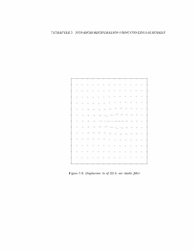
74CHAPTER 5. NON-RIGID REGISTRATIONUSING CONTINUUMMODELS
Figure 5.3: Displacements of 2D linear elastic lter.
5.3. VISCOUS FLUID REGISTRATION 75
We leave it to the reader to determine the lter components for the otherdirections.
A plot of the displacement eld of the 2D lter is shown in gure 5.3. Note,how the lter pulls in material vertically behind the horizontal impulse force.This orthogonal eect is due to the ~r( ~r ~v(~x)) term in the linear elasticdeformation equation and, is important for the viscous eect of the uid.
To show that the application of the lter for linear elastic deformation works,we have made some experiments using the lter as the linear elasticity operator,and compared the results with a Finite Element Model (FEM) of linear elasticity.The results show quite similar deformations. A comparison for a deformationcorresponding to forces applied to 6 nodes in the domain is shown in gure 5.42.
5.3.6 Multi-resolution implementation
Because of the limited span of the discrete lter, we have implemented theviscous uid registration algorithm using the lter in multi-resolution. The uid registration is rst performed on a rough scale. The result of this scale isthen propagated to a ner scale and the uid registration restarted here. Thisprocess is continued down to the nest scale of the scale-space, yielding thenal registration result. All the results shown in this chapter used 3 levels ofresolution.
5.3.7 Results
In the previous sections the original theory of the viscous uid registrationmethod has been described, and a convolution lter was developed to replacethe linear operator in the core routine of the uid registration.
Figure 5.2 shows the result of registering a square to a rectangle. Figure 5.5show the result of registering a circle to a 'C' using viscous uid deformation.The grid shows the curved and very large deformations that are applied to thetemplate. Although the deformation is very large, the topology of the templateis maintained as shown by the rings in the 'bull's eye'. Figure 5.6 shows thedeveloping deformation as the uid circle deforms into the 'C'. These results arevery similar to gures 10.20-23 in [Chr94c].
Figure 5.7 shows the results for two adjacent CT slices. Topologically similarregions have been registered correctly. But, if the images are studied closely,they show that the topology of the original image has been retained to such anextent, that a full registration of the topologically dierent regions has not beenachieved. This is a practical example of the topology-maintaining characteristicsof the viscous uid registration algorithm, ie. the homeomorphic mapping. Asimilar example of registration of two adjacent MR slices is shown in gure 5.8.
Figure 5.9 shows a practical application of 3D uid registration. In thiscase 3 jaws, from the same patient at dierent times, have been extracted from
2The calculations are not exactly comparable since the nite element model used xeddisplacements on the boundary instead of the sliding boundary conditions used by the linearelastic lter.

76CHAPTER 5. NON-RIGID REGISTRATIONUSING CONTINUUMMODELS
Figure 5.4: Complex deformation resulting from three leftward forces in (0,2),(0,3) and (0,4), and three rightward forces in (0,-2), (0,-3) and (0,-4), the centeris (0,0). Left: Using lter. Right: Using FEM.
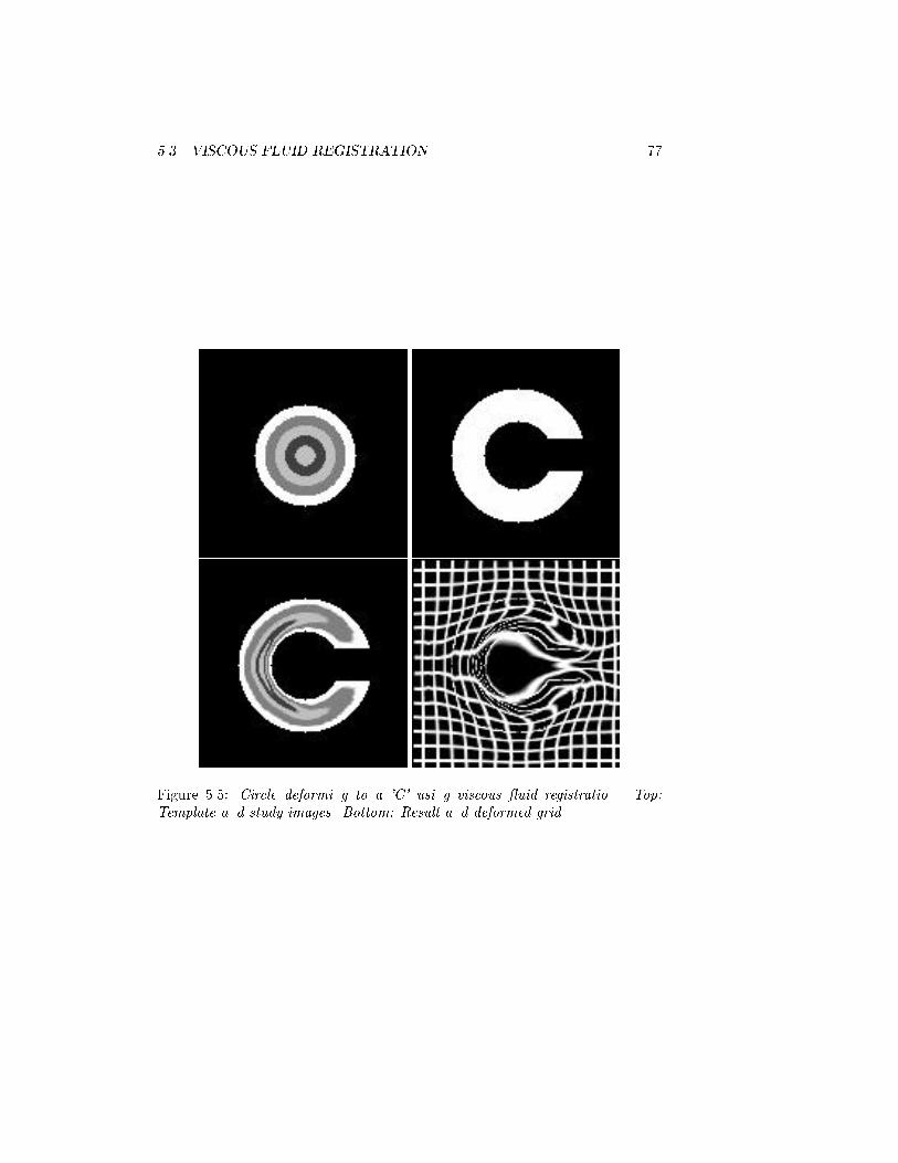
5.3. VISCOUS FLUID REGISTRATION 77
Figure 5.5: Circle deforming to a 'C' using viscous uid registration. Top:Template and study images. Bottom: Result and deformed grid.
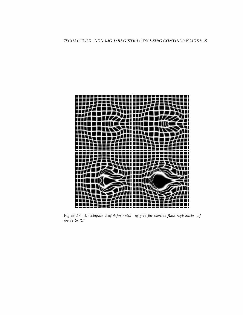
78CHAPTER 5. NON-RIGID REGISTRATIONUSING CONTINUUMMODELS
Figure 5.6: Development of deformation of grid for viscous uid registration ofcircle to 'C'.

5.3. VISCOUS FLUID REGISTRATION 79
Figure 5.7: CT slice registered to another slice using viscous uid model. Top:Template and study images. Bottom: Result and deformed grid.
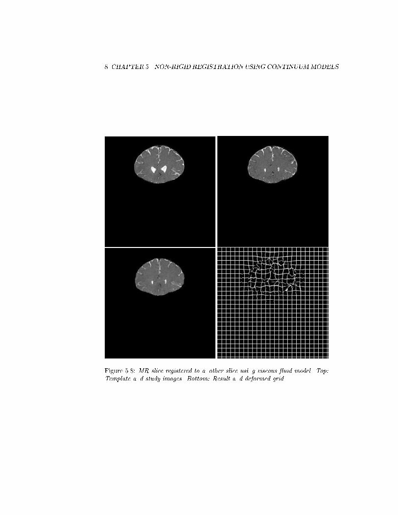
80CHAPTER 5. NON-RIGID REGISTRATIONUSING CONTINUUMMODELS
Figure 5.8: MR slice registered to another slice using viscous uid model. Top:Template and study images. Bottom: Result and deformed grid.
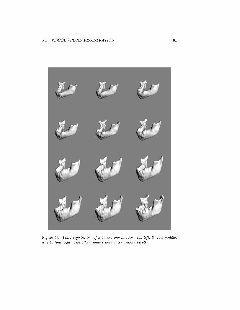
5.3. VISCOUS FLUID REGISTRATION 81
Figure 5.9: Fluid registration of 3 binary jaw images - top left, 2. row middle,and bottom right. The other images show intermediate results.
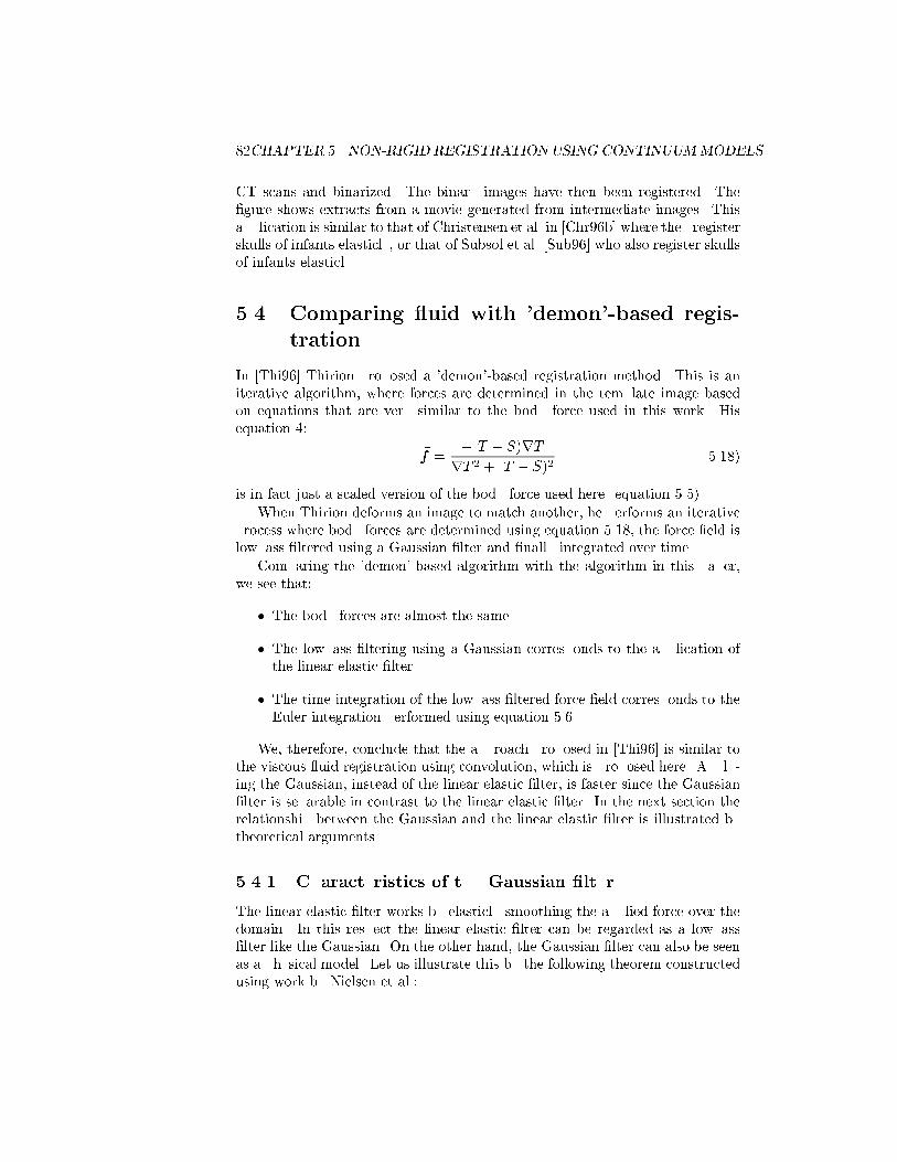
82CHAPTER 5. NON-RIGID REGISTRATIONUSING CONTINUUMMODELS
CT scans and binarized. The binary images have then been registered. Thegure shows extracts from a movie generated from intermediate images. Thisapplication is similar to that of Christensen et al. in [Chr96b] where they registerskulls of infants elasticly, or that of Subsol et al. [Sub96] who also register skullsof infants elasticly.
5.4 Comparing uid with 'demon'-based regis-tration
In [Thi96] Thirion proposed a 'demon'-based registration method. This is aniterative algorithm, where forces are determined in the template image basedon equations that are very similar to the body force used in this work. Hisequation 4:
~f =(T S)rT
rT 2 + (T S)2(5.18)
is in fact just a scaled version of the body force used here (equation 5.5).
When Thirion deforms an image to match another, he performs an iterativeprocess where body forces are determined using equation 5.18, the force eld islowpass ltered using a Gaussian lter and nally integrated over time.
Comparing the 'demon'-based algorithm with the algorithm in this paper,we see that:
The body forces are almost the same.
The lowpass ltering using a Gaussian corresponds to the application ofthe linear elastic lter.
The time integration of the lowpass ltered force eld corresponds to theEuler integration performed using equation 5.6.
We, therefore, conclude that the approach proposed in [Thi96] is similar tothe viscous uid registration using convolution, which is proposed here. Apply-ing the Gaussian, instead of the linear elastic lter, is faster since the Gaussianlter is separable in contrast to the linear elastic lter. In the next section therelationship between the Gaussian and the linear elastic lter is illustrated bytheoretical arguments.
5.4.1 Characteristics of the Gaussian lter
The linear elastic lter works by elasticly smoothing the applied force over thedomain. In this respect the linear elastic lter can be regarded as a lowpasslter like the Gaussian. On the other hand, the Gaussian lter can also be seenas a physical model. Let us illustrate this by the following theorem constructedusing work by Nielsen et al.:

5.4. COMPARING FLUID WITH 'DEMON'-BASED REGISTRATION 83
Theorem 5.3 Finding the Tikhonov regularized solution f(x) of the signalg(x) 2 L2(R) by minimizing the energy:
E[f ] =1
2
Z "(f g)2 +
1Xi=1
i
@i
@xif
2#dx (5.19)
with the coecients (t > 0):
i =ti
i!(5.20)
is the same as convolving the signal g with a Gaussian with the Fourier trans-form:
h =1P
1
i=0ti
i!!2i
= e!2t (5.21)
Proof Nielsen et al. [Nie94], proposition 1 and 3, and result 1. 2
This result shows that convolution with a Gaussian can be seen as nding asolution corresponding to the minimization of an energy functional, ie. a physicalproblem. A similar result exists for the multi-dimensional Gaussian [Nie94].
We note that the solution obtained by convolving with a Gaussian does notsatisfy any specied boundary conditions. Remember that boundary condi-tions are implicitly a condition for the homeomorphic mapping of the domain,since the homeomorphic mapping requires the mapping to be onto. This waspartly satised by requiring the boundary of the domain to be mapped onto theboundary.
In theory the solution using the Gaussian does, therefore, not strictly satisfythe homeomorphic requirement for the transformation. But, in practice it ispossible to circumvent this problem by inserting the image into a larger domain,thus adding a broad boundary to the image in all directions. On the other handthis increases the computational complexity of the problem.
We state another result from the work of Nielsen et al. [Nie96]:
Theorem 5.4 Any analytical function f : R ! R, that is faster than polyno-mially decaying, can be decomposed into a weighted sum of Gaussian derivatives(i)(x; s) with scale parameter s:
f(x) =Xi
i(s)ii!
Hi(x
s)(i)(x; s) (5.22)
where Hi are the Hermite polynomials and the weights i are identied by theHermite moments:
i =
ZHi(
x
s)f(x)dx (5.23)
Proof Nielsen et al. [Nie96, Nie96b]. 2
This theorem indirectly states, that the zero-order approximation of any func-tion that satises the requirements of the theorem is the Gaussian. A similar

84CHAPTER 5. NON-RIGID REGISTRATIONUSING CONTINUUMMODELS
proof exists for the multi-dimensional case [Nie96b]. We can thus understandthe Gaussian as a (very) low-order approximation of the linear elastic lter. Itis, therefore, reasonable to conclude that the approach of Thirion [Thi96] is anapproximation to the viscous uid registration.
When compared to the linear elastic lter it is obvious that the Gaussianlter gives no displacement orthogonal to the direction of a force. The linearlter does this (see gure 5.3) and it is important for the viscous eect of thelter.
5.4.2 The Gaussian versus linear elastic lter for registra-
tion
To investigate the dierences between the two lters, the uid registration al-gorithm has been reimplemented using the Gaussian lter. Experiments usingthe linear elastic and Gaussian lters are shown in gures 5.10, 5.11, and 5.12.
All the results look very similar and quite acceptable, although sometimesdierent when the grids are observed. In particular the circle to 'C' experimentshows that the stretching of the template is not quite the same. Indeed whenone looks closely on the inside of the 'C', the right side of the middle of thestretched bullseye has been compressed more with the Gaussian lter. Thiscould indicate a topological problem for thin anatomical structures.
In addition, the patch to 'C' experiment in gure 5.10 shows that the centralgrid for the Gaussian lter is more dilluted than for the linear elastic lter. Thisis probably caused by the lack of viscous contraction, which the elastic lterintroduces with the ~r( ~r ~v(~x)) term.
Whether these problems are of any concern must depend on the application.
5.5 Timings
Table 5.1 shows the results of the 2D experiments which can be compared to thesimilar experiments reported in [Chr94c]. To be able to compare the numberof iterations for multi-resolution and single-resolution, the number of iterationsfor the multi-resolution work has been calculated, as a weighted sum of theiterations in each resolution. As weight are used the relative voxel distance inthe resolution, since in each resolution the maximum ow distance is scaled toa factor of a voxel.
The table shows that the results of using the convolution approach on asingle workstation, can be compared to those of Christensen et al. on a 128x64DECmpp 12000 Sx/Model 200 massively parallel computer. These timings arestable and consistent with the other results using realistic data.
Using the Gaussian instead of the linear elastic lter gives faster results. But,it is interesting to note that more iterations are required in each resolution. Thiscould be interpretated as a problem related to using the Gaussian lter.
When comparing our results using the linear elastic lter to estimates oftimings on a MIPS R4400 processor [Chr96], it is estimated that a speedup of
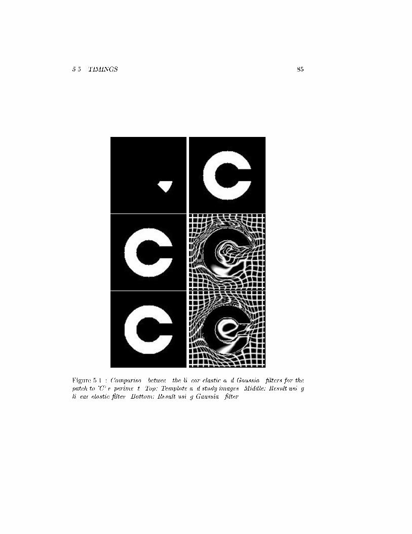
5.5. TIMINGS 85
Figure 5.10: Comparison between the linear elastic and Gaussian lters for thepatch to 'C' experiment. Top: Template and study images. Middle: Result usinglinear elastic lter. Bottom: Result using Gaussian lter.
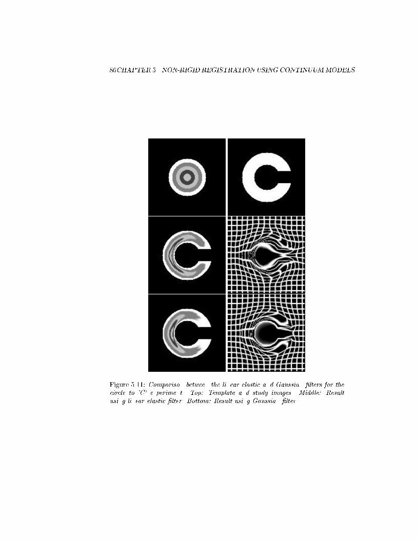
86CHAPTER 5. NON-RIGID REGISTRATIONUSING CONTINUUMMODELS
Figure 5.11: Comparison between the linear elastic and Gaussian lters for thecircle to 'C' experiment. Top: Template and study images. Middle: Resultusing linear elastic lter. Bottom: Result using Gaussian lter.
5.5. TIMINGS 87
Figure 5.12: Comparison between the linear elastic and Gaussian lters forthe square to rectangle experiment. Top: Template and study images. Middle:Result using linear elastic lter. Bottom: Result using Gaussian lter.
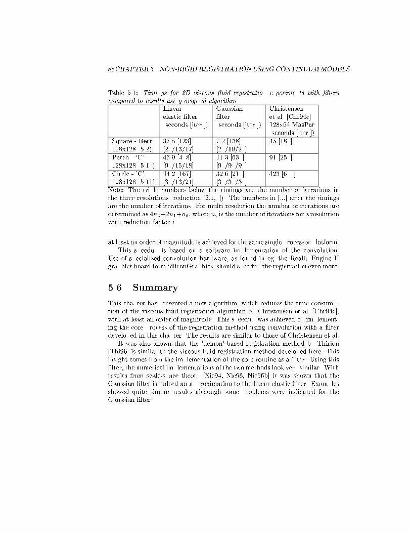
88CHAPTER 5. NON-RIGID REGISTRATIONUSING CONTINUUMMODELS
Table 5.1: Timings for 2D viscous uid registration experiments with lterscompared to results using original algorithm.
Linear Gaussian Christensenelastic lter lter et al. [Chr94c](seconds [iter.]) (seconds [iter.]) 128x64 MasPar
(seconds [iter.])Square - Rect. 37.8 [123] 7.2 [138] 45 [180]128x128 (5.2) [20/13/17] [20/19/20]Patch - 'C' 46.9 [408] 11.3 [630] 91 [250]128x128 (5.10) [90/15/18] [90/90/90]Circle - 'C' 44.2 [167] 32.6 [210] 423 [600]128x128 (5.11) [30/13/21] [30/30/30]
Note: The triple numbers below the timings are the number of iterations inthe three resolutions (reduction [2,1,0]). The numbers in [:::] after the timingsare the number of iterations. For multi-resolution the number of iterations aredetermined as 4n2+2n1+n0, where ni is the number of iterations for a resolutionwith reduction factor i.
at least an order of magnitude is achieved for the same single processor platform.This speedup is based on a software implementation of the convolution.
Use of specialized convolution hardware, as found in eg. the RealityEngine IIgraphics board from SiliconGraphics, should speedup the registration even more.
5.6 Summary
This chapter has presented a new algorithm, which reduces the time consump-tion of the viscous uid registration algorithm by Christensen et al. [Chr94c],with at least an order of magnitude. This speedup was achieved by implement-ing the core process of the registration method using convolution with a lterdeveloped in this chapter. The results are similar to those of Christensen et al.
It was also shown that the 'demon'-based registration method by Thirion[Thi96] is similar to the viscous uid registration method developed here. Thisinsight comes from the implementation of the core routine as a lter. Using thislter, the numerical implementations of the two methods look very similar. Withresults from scale-space theory [Nie94, Nie96, Nie96b] it was shown that theGaussian lter is indeed an approximation to the linear elastic lter. Examplesshowed quite similar results although some problems were indicated for theGaussian lter.
Chapter 6
Non-Rigid Registration
using Bone Growth Model
Bone growth is a biological process far more complex than immediately ex-pected by the layman. Although, the growth is controlled by some very simpleprocesses, the pattern of the growth can be surprisingly sophisticated.
This chapter studies the process of bone growth in the human mandible.Based on the available medical knowledge, a bone growth model is established,and experiments are carried out to determine the validity of the model. Theseexperiments uses a unique data set containing three voxel images of the mandibleof a child, taken at dierent times1.
Being able to model the growth of the facial bones is both interesting for un-derstanding the development of the cranio-facial complex, and for understandingthe eects of cranio-facial surgery on children. After children with growth de-fects have undergone surgery to restore normal function and appearance, thebones continue to grow. This growth often introduces new deformations andnew surgery has to be performed.
It is, therefore, important to understand the growth of the bones. Optimally,it would be useful for the surgeon to be able, not only to predict the instanta-neous result of the surgery (as discussed in the next chapter), but also to predictthe evolution of the face after surgery. Using such knowledge, the surgeon couldpossibly anticipate this development and correct for it in advance.
The process of modeling the growth can be seen as a registration problem,and the discussion follows the notation and semantics of the general registrationmethodology used in the previous chapters. Indeed the inspiration, for the de-velopment of the growth based registration algorithm, came from the experiencewith uid registration of the jaw images (gure 5.9).
1This data set was kindly made available by Prof. Sven Kreiborg of the School of Dentistry,University of Copenhagen, Denmark.
89
90CHAPTER 6. NON-RIGID REGISTRATIONUSING BONEGROWTHMODEL
6.1 Non-rigid registration as a physical problem
Non-rigid registration is used to register images that are dierent. As 'non-rigid'indicates, more than just a simple superposition of the images is required to geta complete correspondence, and some sort of deformation must be included inthe transformation, to map dissimilar images onto each other.
Optimally, the non-rigidness of the transformation allow a full correspon-dence to be determined, and at the same time limit excessive deformations byincluding some sort of regularization eect.
As illustrated in the previous chapter, most non-rigid registration methodsare directly or indirectly based on elastic or viscous- uid models. Althoughmany methods do not use the terminology of these continuum models, theyfollow the same ideas algorithmicly. As an example, the application of theGaussian lter, to a driving force eld, is the same as Thikonov regularizationof this eld [Nie94], and thus the application of a physical model similar to anelastic deformation.
The use of elastic and viscous uid models for registration of images hasoften been criticized, because they represent the application of a physical model,which does not re ect the actual physical development between the images.
A correct physical model, for registration of images of the brain of two in-dividuals, would re ect the actual biologic and genetic development of thesebrains. Since a common genetic basis exists for these brains, it should, theoreti-cally, be possible to create a development model for the two brains down throughhistory to a common ancestor. Using this development model a correspondencecould be created.
The dierence between the traditional registration models and the idea ofa physically correct model of development, is illustrated in gure 6.1. Rigidregistration methods basicly register images to derivatives of themselves. Thetraditional non-rigid registration methods attempt to model the dierence be-tween two images, using an arbitrary physical model, which does not re ect theactual physical process. The development methods, on the other hand, use theactual physical process as the model of change.
One of the important advantages, of using a physically correct model, is theability to simulate what happens between the images. Where traditional non-rigid methods only provide a correspondence between the images, the physicallyvalid models describe the actual development, which can then be simulated.Naturally, these models have generally been viewed as impossible, althoughconceptually interesting.
In this chapter a physically valid development model, for non-rigid registra-tion of time sequence images of the human mandible is developed. With a modelof physical bone growth, images are registered by allowing the initial image togrow to the second image. The initial and nal images are used as boundaryconditions.
A set of three images of the mandible of the same child at dierent times,is used to validate the growth model (see gure 6.2). These images have beenacquired at the age of 9, 21 months and 7 years.

6.1. NON-RIGID REGISTRATION AS A PHYSICAL PROBLEM 91
Image 2
Non-rigidregistrationusing arbitraryphysical model
registrationRigid
Unknown physical model
Elastic or fluid model
Known physical model
Simulation
Non-rigidregistrationusing validphysical model
Image 1
Figure 6.1: Dierent registration methods and their use of physically valid orinvalid models of the change between two images.
Figure 6.2: Images of the mandible of a child at the age of 9, 21 months and 7years.
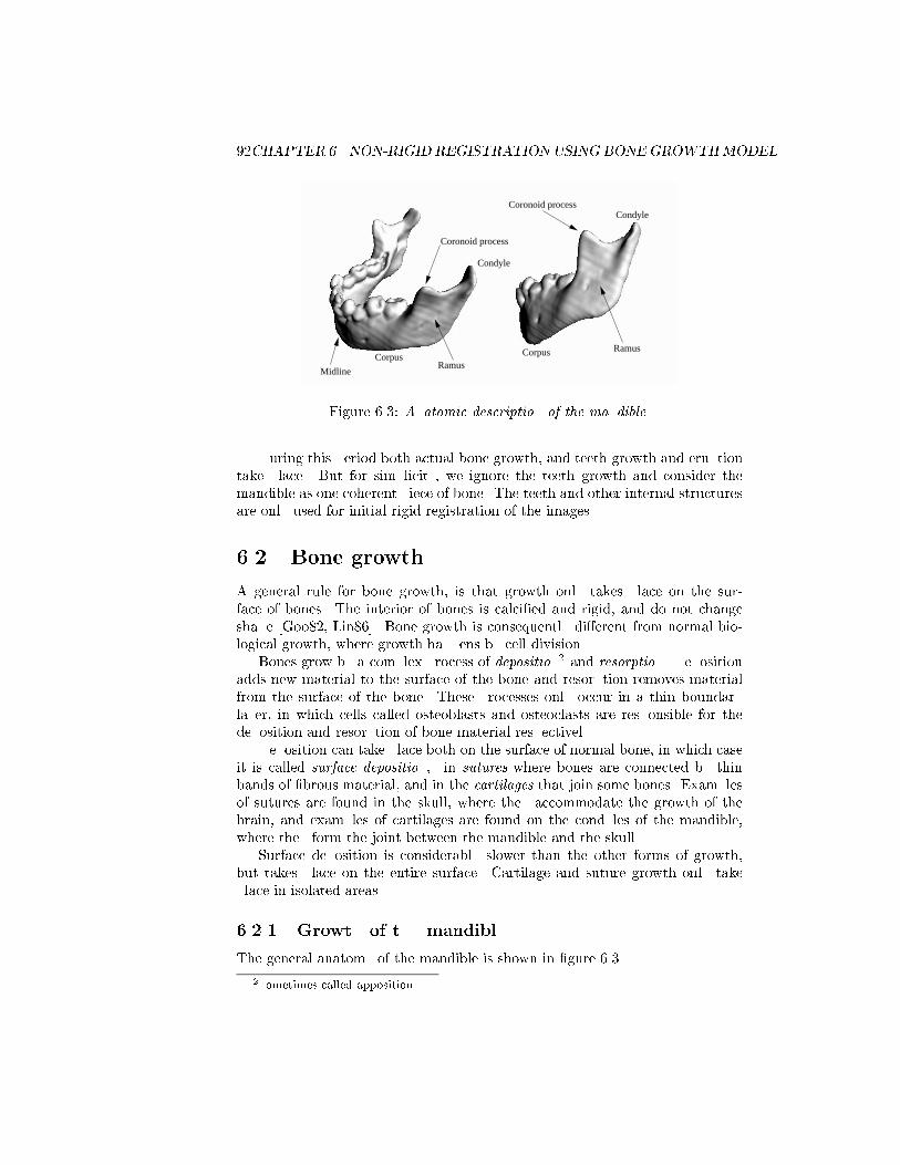
92CHAPTER 6. NON-RIGID REGISTRATIONUSING BONEGROWTHMODEL
CorpusRamus
Coronoid processCondyle
RamusCorpus
Condyle
Coronoid process
Midline
Figure 6.3: Anatomic description of the mandible.
During this period both actual bone growth, and teeth growth and eruptiontake place. But for simplicity, we ignore the teeth growth and consider themandible as one coherent piece of bone. The teeth and other internal structuresare only used for initial rigid registration of the images.
6.2 Bone growth
A general rule for bone growth, is that growth only takes place on the sur-face of bones. The interior of bones is calcied and rigid, and do not changeshape [Goo82, Lin86]. Bone growth is consequently dierent from normal bio-logical growth, where growth happens by cell division.
Bones grow by a complex process of deposition2 and resorption. Depositionadds new material to the surface of the bone and resorption removes materialfrom the surface of the bone. These processes only occur in a thin boundarylayer, in which cells called osteoblasts and osteoclasts are responsible for thedeposition and resorption of bone material respectively.
Deposition can take place both on the surface of normal bone, in which caseit is called surface deposition, in sutures where bones are connected by thinbands of brous material, and in the cartilages that join some bones. Examplesof sutures are found in the skull, where they accommodate the growth of thebrain, and examples of cartilages are found on the condyles of the mandible,where they form the joint between the mandible and the skull.
Surface deposition is considerably slower than the other forms of growth,but takes place on the entire surface. Cartilage and suture growth only takeplace in isolated areas.
6.2.1 Growth of the mandible
The general anatomy of the mandible is shown in gure 6.3.
2Sometimes called apposition.

6.3. NON-RIGID REGISTRATIONOFMANDIBLES USING BONEGROWTHMODEL93
Inferior dental nerve channelInner cortical surface
Third molar
Third molar
Inner cortical surface
Figure 6.4: Stable features in the mandible.
Up to the second half of the rst year the mandible has cartilage in themidline. But after this period the two halves are connected and the cartilagedisappears. The mandible is then a single bone, with cartilages on the twocondyles (the mandibular condylar cartilages).
Growth of the mandible takes place by growth in the condylar cartilages, andby surface deposition and resorption on the remaining surface of the mandible.
That the mandible only grows by surface processes can seem surprising,considering the large size dierence between the jaw of a child and an adult.But implant studies by Bjork [Bj61, Bj63] and Bjork and Skieller [Bj72, Bj77]have shown this model of the growth process to be valid at least for the corpus.The growth pattern of the condyles is still under discussion.
6.2.2 Stable structures
Since the interior of the mandible does not grow, it should be expected thatstable structures could be detected here.
Indeed based on his implant studies, Bjork [Bj69] suggested the inferiordental nerve channel, the inner cortical surface of the symphysis, the lowermargin of the third molar tooth germ before it erupts, and the tip of the chinas stable features of the mandible (see gure 6.4).
There is general agreement on these features, although the third molar isonly stable during the period, in which it has not started developing roots. Itcan, therefore, not be used in studies over many years.
6.3 Non-rigid registration of mandibles using bonegrowth model
Using the information about the growth of the mandible, this section establishesa mathematical model of the growth process, and a simulation algorithm, which
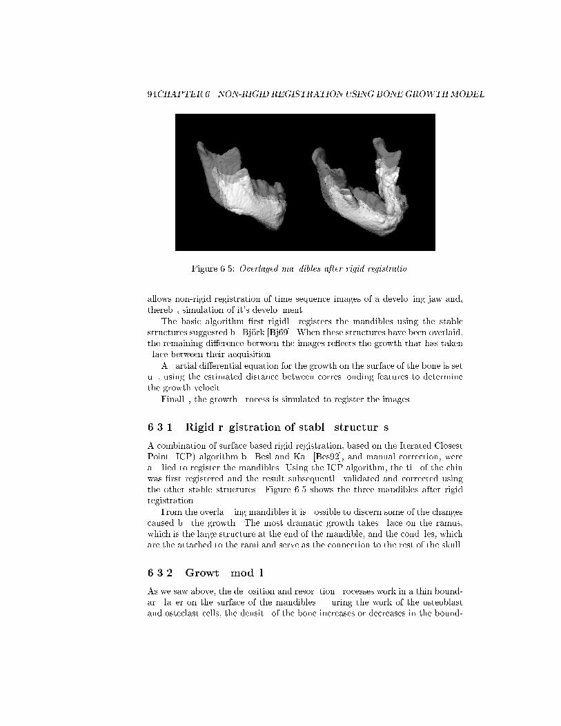
94CHAPTER 6. NON-RIGID REGISTRATIONUSING BONEGROWTHMODEL
Figure 6.5: Overlayed mandibles after rigid registration.
allows non-rigid registration of time sequence images of a developing jaw and,thereby, simulation of it's development.
The basic algorithm rst rigidly registers the mandibles using the stablestructures suggested by Bjork [Bj69]. When these structures have been overlaid,the remaining dierence between the images re ects the growth that has takenplace between their acquisition.
A partial dierential equation for the growth on the surface of the bone is setup, using the estimated distance between corresponding features to determinethe growth velocity.
Finally, the growth process is simulated to register the images.
6.3.1 Rigid registration of stable structures
A combination of surface based rigid registration, based on the Iterated ClosestPoint (ICP) algorithm by Besl and Kay [Bes92], and manual correction, wereapplied to register the mandibles. Using the ICP algorithm, the tip of the chinwas rst registered and the result subsequently validated and corrected usingthe other stable structures. Figure 6.5 shows the three mandibles after rigidregistration.
From the overlapping mandibles it is possible to discern some of the changescaused by the growth. The most dramatic growth takes place on the ramus,which is the large structure at the end of the mandible, and the condyles, whichare the attached to the rami and serve as the connection to the rest of the skull.
6.3.2 Growth model
As we saw above, the deposition and resorption processes work in a thin bound-ary layer on the surface of the mandibles. During the work of the osteoblastand osteclast cells, the density of the bone increases or decreases in the bound-

6.3. NON-RIGID REGISTRATIONOFMANDIBLES USING BONEGROWTHMODEL95
−1
0
Ω
Γ
Γ1 Γ
Figure 6.6: Denition of growth domain.
ary layer until bone has either been completely deposited or resorped. Theboundary layer then moves, and the process restarts.
To model this, the bone density (x; t) 2 [0; 1] is used as the primary vari-able. Bone is dened as (x; t) = 1 and air is dened as (x; t) = 0. Thus, thedenition of the bone body becomes:
= fxj(x; t) = 1g (6.1)
Using the same notation as in the previous chapter, we dene the initial imageas the template image T (x) 2 [0; 1] and the desired end-state as the study imageS(x) 2 [0; 1]. The initial domain can therefore be written as:
= fxj(x; 0) = T (x)g (6.2)
The registration problem is formulated as changing the density map using amodel of growth, so that (x; tend) = S(x) where tend is the time of full regis-tration.
The boundary of the domain is denoted ~ (see gure 6.6), and consists of astable part ~0, where the template and study boundaries match, and unstableparts ~1, and ~1 where deposition and resortion take place respectively:
~ = ~0 + ~1 + ~1~0 = fx 2 ~ j T (x) = S(x)g~1 = fx 2 ~ j T (x) < S(x) ^ (x; t) 2 [0; 1[g
~1 = fx 2 ~ j T (x) > S(x) ^ (x; t) 2]0; 1]g (6.3)
For completeness we dene the boundary as having a thickness > 0.We now proceed to dene the partial dierential equation (PDE) governing
the growth process. The general requirements for this PDE is that change indensity should happen only for x 2 ~1 + ~1, and that the change in densityshould re ect the velocity of the actual growth. The PDE is dened as:
@(x; t)
@t=
8<:
cvg(x; t) x 2 ~1cvg(x; t) x 2 ~10 x 2 ~0 [ ~
(6.4)
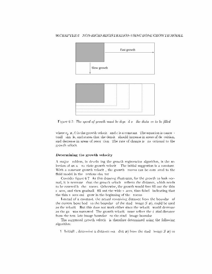
96CHAPTER 6. NON-RIGID REGISTRATIONUSING BONEGROWTHMODEL
Slow growth
Fast growth
Figure 6.7: The speed of growth must be depend on the distance to be lled.
where vg(x; t) is the growth velocity and c is a constant. The equation is concep-tually simple, and states that the density should increase in areas of deposition,and decrease in areas of resorption. The rate of change is proportional to thegrowth velocity.
Determining the growth velocity
A major problem, in developing the growth registration algorithm, is the se-lection of an appropriate growth velocity. The initial suggestion is a constant.With a constant growth velocity, the growth process can be compared to the uid model in the previous chapter.
Consider gure 6.7. As this drawing illustrates, for the growth to look nor-mal, it is necessary that the growth velocity re ects the distance, which needsto be covered by the process. Otherwise, the growth would rst ll out the thinspaces, and then gradually ll out the wide spaces, thus falsely indicating thatthe thin spaces only grow in the beginning of the process.
Instead of a constant, the actual remaining distance from the boundary ofthe current bone body to the boundary of the study image S(x), could be usedas the velocity. But this does not work either since the velocity would decreaseas the gap was narrowed. The growth velocity must re ect the initial distancefrom the template image boundary to the study image boundary.
The suggested growth velocity is therefore determined using the followingalgorithm:
1. Initially, determine a distance map dist(x) from the study image S(x) to
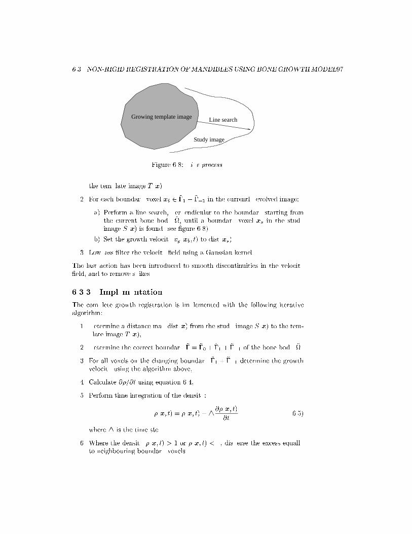
6.3. NON-RIGID REGISTRATIONOFMANDIBLES USING BONEGROWTHMODEL97
Line search
Study image
Growing template image
Figure 6.8: Line process.
the template image T (x).
2. For each boundary voxel xb 2 ~1 + ~1 in the currently evolved image:
(a) Perform a line search, perpendicular to the boundary starting fromthe current bone body ~, until a boundary voxel xs in the studyimage S(x) is found (see gure 6.8).
(b) Set the growth velocity vg(xb; t) to dist(xs).
3. Lowpass lter the velocity eld using a Gaussian kernel.
The last action has been introduced to smooth discontinuities in the velocityeld, and to remove spikes.
6.3.3 Implementation
The complete growth registration is implemented with the following iterativealgorithm:
1. Determine a distance map dist(x) from the study image S(x) to the tem-plate image T (x),
2. Determine the correct boundary ~ = ~0 + ~1 + ~1 of the bone body ~.
3. For all voxels on the changing boundary ~1 + ~1 determine the growthvelocity using the algorithm above,
4. Calculate @=@t using equation 6.4,
5. Perform time integration of the density:
(x; t) = (x; t) +4@(x; t)
@t(6.5)
where 4 is the time step.
6. Where the density (x; t) > 1 or (x; t) < 0, disperse the excess equallyto neighbouring boundary voxels.
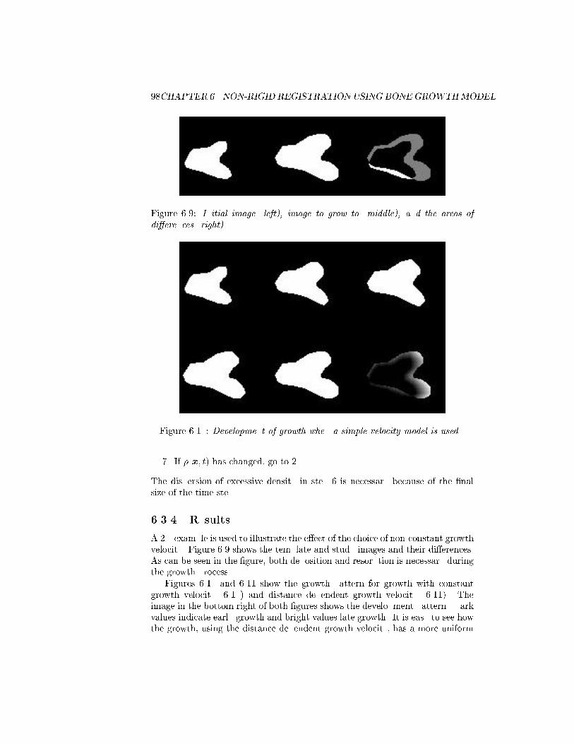
98CHAPTER 6. NON-RIGID REGISTRATIONUSING BONEGROWTHMODEL
Figure 6.9: Initial image (left), image to grow to (middle), and the areas ofdierences (right).
Figure 6.10: Development of growth when a simple velocity model is used.
7. If (x; t) has changed, go to 2
The dispersion of excessive density in step 6 is necessary because of the nalsize of the time step.
6.3.4 Results
A 2D example is used to illustrate the eect of the choice of non-constant growthvelocity. Figure 6.9 shows the template and study images and their dierences.As can be seen in the gure, both deposition and resorption is necessary duringthe growth process.
Figures 6.10 and 6.11 show the growth pattern for growth with constantgrowth velocity (6.10) and distance dependent growth velocity (6.11). Theimage in the bottom right of both gures shows the development pattern. Darkvalues indicate early growth and bright values late growth. It is easy to see howthe growth, using the distance dependent growth velocity, has a more uniform
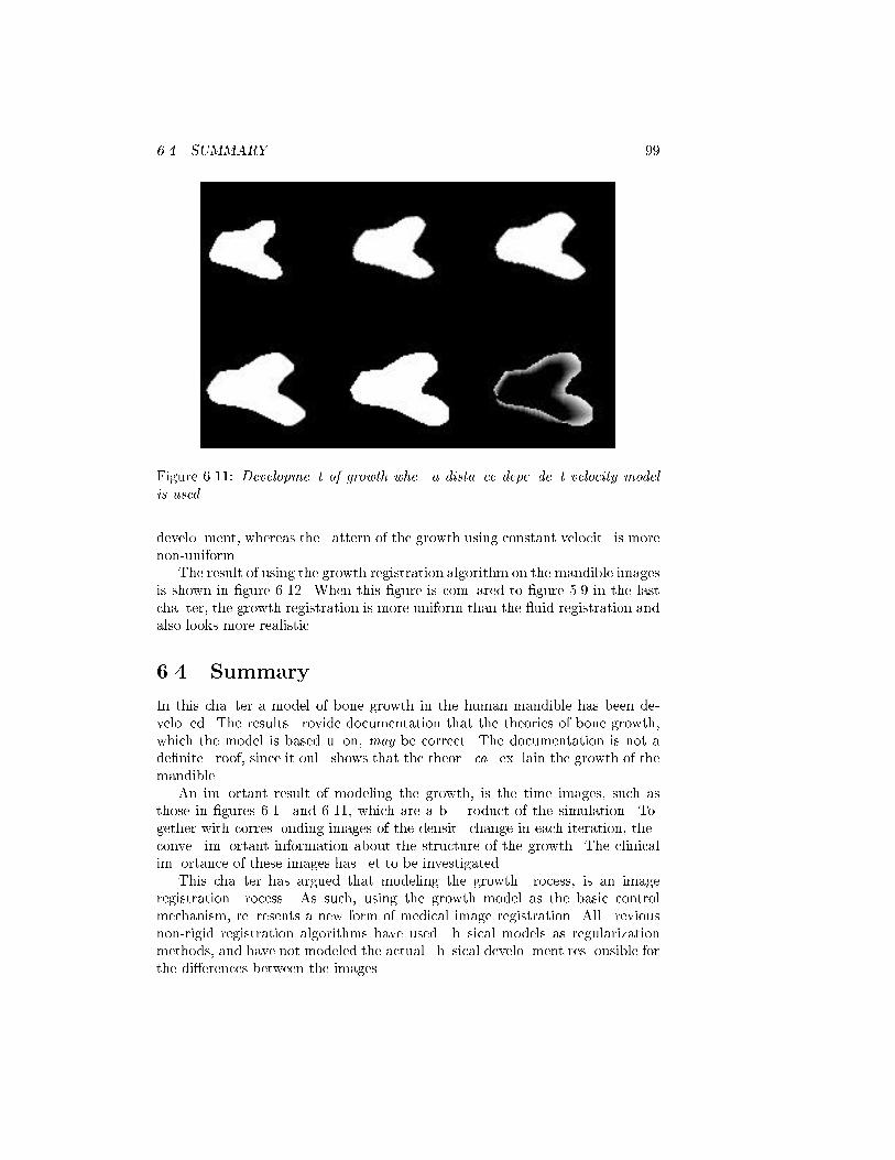
6.4. SUMMARY 99
Figure 6.11: Development of growth when a distance dependent velocity modelis used.
development, whereas the pattern of the growth using constant velocity is morenon-uniform.
The result of using the growth registration algorithm on the mandible imagesis shown in gure 6.12. When this gure is compared to gure 5.9 in the lastchapter, the growth registration is more uniform than the uid registration andalso looks more realistic.
6.4 Summary
In this chapter a model of bone growth in the human mandible has been de-veloped. The results provide documentation that the theories of bone growth,which the model is based upon, may be correct. The documentation is not adenite proof, since it only shows that the theory can explain the growth of themandible.
An important result of modeling the growth, is the time images, such asthose in gures 6.10 and 6.11, which are a by-product of the simulation. To-gether with corresponding images of the density change in each iteration, theyconvey important information about the structure of the growth. The clinicalimportance of these images has yet to be investigated.
This chapter has argued that modeling the growth process, is an imageregistration process. As such, using the growth model as the basic controlmechanism, represents a new form of medical image registration. All previousnon-rigid registration algorithms have used physical models as regularizationmethods, and have not modeled the actual physical development responsible forthe dierences between the images.
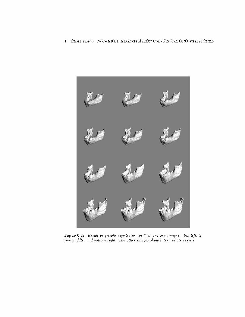
100CHAPTER 6. NON-RIGID REGISTRATION USING BONEGROWTHMODEL
Figure 6.12: Result of growth registration of 3 binary jaw images - top left, 2.row middle, and bottom right. The other images show intermediate results.
Chapter 7
Soft Tissue Modeling in
Surgery Simulation
Just like ight simulators are essential today in the education of aircraft pilots,surgery simulators are expected to have an important impact on the educationof surgeons in the future [Sa93].
Currently training of surgeons is either performed using animals, cadavers,or actual human patients. But, it is expected that these training methodswill be restricted in the future. Animal protection groups are pressuring themedical industry to restrict the use of animals for experiments, cadavers aregenerally problematic, and the use of direct training (under supervision) onhuman patients will probably increasingly be limited by insurance problems andpatient scepticism. In addition, the facilities necessary for training on animalsare quite expensive.
Virtual reality techniques are, therefore, being developed to replace experi-mentation on live objects with simulated environments. In particular, the eldsof cranio-facial and minimally invasive surgery have seen the development ofsome initial surgery simulators.
7.1 Cranio-facial surgery simulation
Cranio-facial surgery is used to change the bone structure of a patient's face.The purpose of this kind of surgery, is to enhance the appearance of the pa-tient or to restore normal function, when abnormal bone growth has resulted inrestriction of body function or development.
During surgery, parts of the cranio-facial bones are separated from the re-mainder, and rearranged like building blocks, by the surgeon. Naturally, exten-sive planning takes place to determine the best procedure.
This planning is usually performed using x-ray cephalometric techniques andreconstructed CT images. Some cranio-facial teams are using solid modeling
101
102CHAPTER 7. SOFT TISSUE MODELING IN SURGERY SIMULATION
software (eg. [Lo94]), but most use manual ad-hoc methods during the planningphase.
Although the surgery generally aims at improving the overall facial appear-ance of the patient, traditionally only the eects on the bone structures havebeen considered systematicly during planning. The relationship to the soft tis-sue surface of the patient has often been left to experience and guessing.
But, in recent years promising work has been done to develop simulationsoftware, which can model the soft tissue changes, that are the result of changesin the underlying bone structure of the patient.
The requirements for such simulators are primarily realism, and since speedis not an important concern, most of the attention has been directed at thedevelopment of realistic soft tissue models.
These simulators are therefore not realistic models of the surgery situation,but rather software tools for modeling and planning surgery.
7.2 Minimally invasive surgery simulation
Minimally invasive procedures such as endoscopy and laparascopy are replacingmore and more normal procedures, with extensive benets for both patients andhospitals in terms of reduced hospitalization time and fewer complications.
These procedures all share the characteristic that the surgeon's interfaceto the patient is limited to a TV screen, and tools that are inserted into thepatient through either natural body openings or small incisions. The interfaceis, consequently, dramatically reduced in comparison to open surgery, where thesurgeon has direct contact to body tissues and uids.
Because of the simplicity of the patient/surgeon interface, surgery simulatorsare relatively easier to develop for minimally invasive surgery. At the same timespecial motoric skills are needed for this kind of surgery, which can only beacquired by extensive practice with the actual instruments. Together thesefactors have driven the research into virtual reality techniques to replace thecurrent use of either animals or simplistic 'brick and block' setups for trainingof surgeons.
Since virtual reality simulators require real-time response, research has con-centrated on developing high-speed simplied elastic models and computer graph-ics.
7.3 Technical requirements
The requirements of a general surgery simulator can be characterized by thefollowing three demands:
Computer graphics: Graphics is needed to render realistic views of the vir-tual surgery scene, and provide the surgeon with a visual illusion of reality.
Haptic interface: A haptic interface is provided through the instruments andtools which the surgeon uses to work on the virtual reality simulator. By

7.3. TECHNICAL REQUIREMENTS 103
tracking the position of these tools and sensing their state, the computeris able to determine the actions of the surgeon in the virtual scene, andact accordingly.
In addition, the haptic interface provides the surgeon with a physical sen-sation of touching and sensing objects in the scene using force-feedbacktechniques. The haptic interface thus represents the sense of touch illusionof reality.

104CHAPTER 7. SOFT TISSUE MODELING IN SURGERY SIMULATION
Physical modeling: Physical models provide the surgeon with a behaviouralillusion of reality. By modeling the visco-elastic behaviour of human skin,the uid ow of blood from a wound etc., these models ensure that thevirtual scene re ects the expectations of the behaviour of the physicalreality.
Computer graphics have been extensively developed over the last decades, andis today quite sucient for surgery simulation systems. Only speed and price isstill problematic, but the general development of hardware leaves no doubt thatit is only a question of time before the necessary computers will be available atreasonable prices.
Haptic interface devices for minimally invasive surgery simulation can bebought commercially, and although benets of continued development are ex-pected, the quality is already sucient for many purposes.
Physical models represent the biggest obstacle today in surgery simulation.In particular, the development of real-time elastic models of human soft tissueis essential for the continued evolution of surgery simulation systems.
In engineering and physics, elastic models have been developed during thelast century, and the immediate idea would be to apply these models directlyfor surgery simulation. Unfortunately, this is only feasible for the cranio-facialsimulators that were described above.
Traditional elastic mathematical models have been developed with high em-phasis on precision, and solution time has only had secondary importance. Sincecranio-facial surgery simulators have similar requirements, the traditional meth-ods can be used to some degree. But for real-time simulators, such as those usedfor minimally invasive surgery, the demands are often contrary to those of engi-neering and physics models. Virtual reality surgery simulation models are beingdeveloped with emphasis on speed. For training simulators the requirement forprecise physical models is much less than the demand for visually satisfying andfast models.
Because of the dierent demands of cranio-facial surgery simulation andvirtual reality systems, the development currently follows two parallel tracks asillustrated in gure 7.1. Cranio-facial simulation models use relatively realistic,but time-consuming models, and virtual reality systems use very simple real-time models. It is probable that these tracks will converge in the future as morepowerful computers become available.
The contribution of this thesis, in surgery simulation, is centered on thedevelopment of visually satisfying elastic models for real-time deformation ofhuman soft tissue. This work is described in the next chapter.
7.4 Previous work
Without going into specic technical details this section reviews the most im-portant work on soft tissue modeling in surgery simulation.

7.4. PREVIOUS WORK 105
15-30 frames / secondVirtual reality systems
Off-line calculationCranio-facial surgery
Merge ?
Real-time modelsRealistic models
Soft tissue modeling
Figure 7.1: Parallel development of soft tissue models for realistic (cranio-facialsurgery) and real-time models (virtual reality training systems).
7.4.1 Cranio-facial surgery simulation models
Early work using solid modeling techniques have been reported by Yasuda etal. [Yas90], Satoh et al. [Sat92], Caponetti et al. [Cap93], Lo et al. [Lo94], andDelingette et al. [Del94]. Delingette et al. used 2-simplex surface meshes [Del94b]to represent the surface of the skull, and also reported on some preliminaryexperiments using 3-simplex meshes as models of the soft tissue between the2-simplex meshes of the skull and the skin.
In his Ph.D. thesis Pieper [Pie92, Pie92b] presented work on a completesystem for simulating plastic surgery. His system used a volumetric linear elasticnite element model for the skin, and showed validation results comparing realplastic surgery results to predictions obtained using the system.
Interesting work has been reported by Waters and Terzopoulos on facialanimation [Wat87, Wat91, Ter91b, Wat92, Ter93, Lee93, Lee95] in which theycreated non-linear mass-spring models of the facial soft tissues. By addingmuscles, and modeling the muscle activity for general human expressions, theydeveloped the ability to animate human expressions.
Keeve et al. [Kee95b, Kee95, Kee96c] have been strongly in uenced by thiswork. They developed a similar system in which they created individualizedmodels from CT scans and added the ability to perform surgical procedureson the bone structures using interactive computer graphics. By moving sepa-rated bone pieces and modeling the corresponding soft tissue deformation, theyobtained an estimate of the resulting facial changes for the particular surgery.Some validation results have been reported.
In [Kee95b, Kee95, Kee96c] Keeve et al. used the mass-spring models orig-
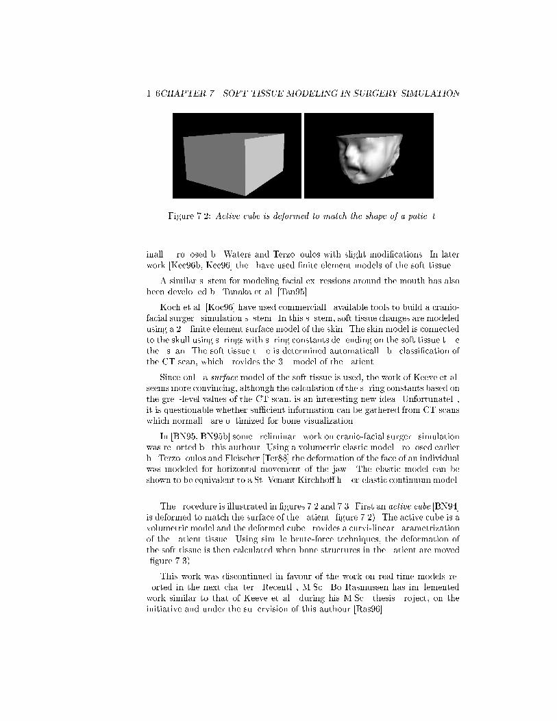
106CHAPTER 7. SOFT TISSUE MODELING IN SURGERY SIMULATION
Figure 7.2: Active cube is deformed to match the shape of a patient.
inally proposed by Waters and Terzopoulos with slight modications. In laterwork [Kee96b, Kee96] they have used nite element models of the soft tissue.
A similar system for modeling facial expressions around the mouth has alsobeen developed by Tanaka et al. [Tan95].
Koch et al. [Koc96] have used commercially available tools to build a cranio-facial surgery simulation system. In this system, soft tissue changes are modeledusing a 2D nite element surface model of the skin. The skin model is connectedto the skull using springs with spring constants depending on the soft tissue typethey span. The soft tissue type is determined automatically by classication ofthe CT scan, which provides the 3D model of the patient.
Since only a surface model of the soft tissue is used, the work of Keeve et al.seems more convincing, although the calculation of the spring constants based onthe grey-level values of the CT scan, is an interesting new idea. Unfortunately,it is questionable whether sucient information can be gathered from CT scanswhich normally are optimized for bone visualization.
In [BN95, BN95b] some preliminary work on cranio-facial surgery simulationwas reported by this authour. Using a volumetric elastic model proposed earlierby Terzopoulos and Fleischer [Ter88] the deformation of the face of an individualwas modeled for horizontal movement of the jaw. The elastic model can beshown to be equivalent to a St. Venant Kirchho hyper-elastic continuum model.
The procedure is illustrated in gures 7.2 and 7.3. First an active cube [BN94]is deformed to match the surface of the patient (gure 7.2). The active cube is avolumetric model and the deformed cube provides a curvi-linear parametrizationof the patient tissue. Using simple brute-force techniques, the deformation ofthe soft tissue is then calculated when bone structures in the patient are moved(gure 7.3).
This work was discontinued in favour of the work on real-time models re-ported in the next chapter. Recently, M.Sc. Bo Rasmussen has implementedwork similar to that of Keeve et al. during his M.Sc. thesis project, on theinitiative and under the supervision of this authour [Ras96].
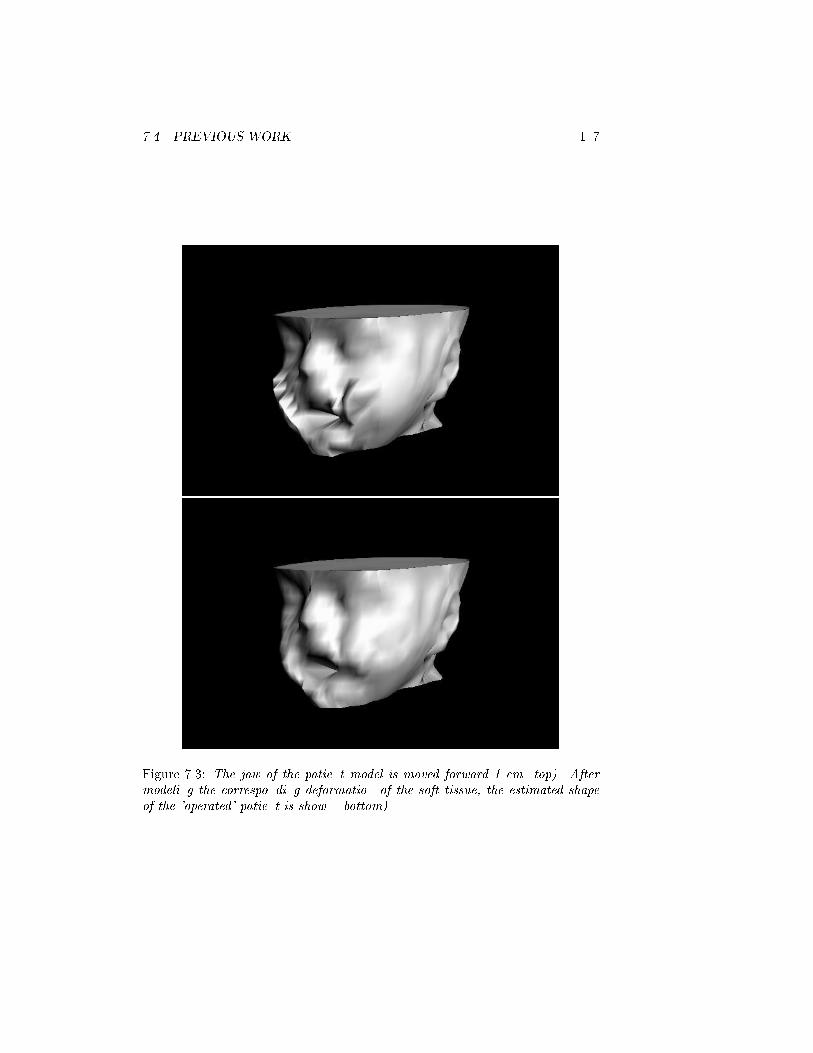
7.4. PREVIOUS WORK 107
Figure 7.3: The jaw of the patient model is moved forward 1 cm (top). Aftermodeling the corresponding deformation of the soft tissue, the estimated shapeof the 'operated' patient is shown (bottom).
108CHAPTER 7. SOFT TISSUE MODELING IN SURGERY SIMULATION
7.4.2 Real-time surgery simulation models
The demands of real-time performance have forced most researchers to developor adapt very simplistic models of elastic deformation to the needs of surgerysimulation. Eg. instead of using implicit solution methods which require thesolution of matrix systems, explicit models (aka. mass-spring models) havefrequently been used. Although these models suer from poor precision andstability problems, they are very easy to implement and yield reasonable speeds.In addition they can be easily implemented on parallel processors.
Cover et al. [Cov93] were the rst to present real-time models for surgerysimulation. They used a simple surface-based mass-spring model to simulatedeformation of a gall-bladder.
Kuhnapfel, Deussen, and Kuhn [Kue93, Kue94, Kue95, Deu95, Ku96] haveimplemented mass-springmodels in their KISMET simulation system. Althoughthe models basicly are surface models, they introduce volumetric behaviour byincluding parent nodes which connect nodes on dierent sides of an object.Interesting work on determining the optimal positioning of nodes and theirmasses were presented in [Deu95] in which they used simulated annealing tond the optimal conguration. The resulting system, eg. as presented in [Ku96],looks quite convincing.
Surface models are also used in the commercial Teleos software developedby HT Medical, Inc., Maryland, USA1. They use tubular spline surface modelsand can only model simple structures derived from the tubular topology (eg.arteries, gall-bladder). On the other hand this system is the rst commercialsimulation toolkit, and functional additions can probably be expected in thefuture.
Implicitly solved nite element systems have been used in the on-going paral-lel work of Bro-Nielsen [BN95b, Cot96, BN96c, BN96d] and Cotin et al. [BN95b,Cot96, BN96c, Cot96]. The rst work on the use of implicit nite element mod-els of linear elastic models was presented in [BN95b, Cot96]. The next chapterdescribes later work by Bro-Nielsen [BN96c, BN96d] where a technique calledcondensation was introduced to reduce the complexity of volumetric nite el-ement models. The resulting models are called Fast Finite Element (FFE)models.
The most advanced use of nite elements has been presented by Sagaret al. [Sag94]. Their eye surgery simulator used a non-linear incompressibleMooney-Rivlin elastic model with nite elements to model deformation of theeye. The nite element solution to this kind of model is normally computation-ally expensive, and it is currently only in such very specialized simulators it ispossible to use these models.
7.4.3 Work for the future
Just as line drawing were replaced by pixel drawing for 2D graphics, todayvolume rendering is used more and more instead of polygonal models for visu-
1Previously known as High Techsplanations, Inc.

7.5. SUMMARY 109
alization of 3D volume data.All the simulators described above basicly use polygonal models such as
triangle surfaces or tetrahedral nite element meshes. It is thus an interestingthought that these polygonal models one day might be replaced by volumetricvoxel models.
In an eye-opening paper [Gib95], Gibson suggested the use of voxel-basedmodels for deformable models. Gibson demonstrated how intuitively simplesuch tasks as collision detection become in this environment.
Unfortunately, the stumbling block for development of such models is therendering speed which follows that of traditional volume rendering. Some speed-up can be achieved by only rendering objects in the scene that change shape orposition, but the low speed is still prohibitive.
In addition, deformation of volumetric models is a considerable problem.But in contrast to the normal nite element mesh models, the size of the meshelements is equal to the sampling size of the voxel grid, and techniques, such asthose developed in chapter 5 for viscous- uid motion modeling, could probablybe used for solving the voxel-mesh deformation problem.
Although Gibson only presented 2D deformation experiments, the basic ideaof using voxel-based models seems very promising.
7.5 Summary
In this chapter the basic lines of research into surgery simulation systems havebeen presented. The technical problems were discussed and previous work wasdescribed. The next chapter presents the contribution of this thesis to surgerysimulation models in the form of Fast Finite Element models.

110CHAPTER 7. SOFT TISSUE MODELING IN SURGERY SIMULATION

Chapter 8
Real-time Deformable
Models for Surgery
Simulation
The main problem in real-time surgery simulation, is modeling the deformationof solid volumetric objects. These objects are typicly human organs or tissues,which often have quite irregular shape and complex visco-elastic behaviour.
Some of the previous work have used surface models as the basic model-ing method [Cov93, HT95], and realistic tissue models have only been appliedin very specialized simulators, such as the eye-surgery simulator of Sagar etal. [Sag94].
The problem with surface models, is that they do not behave like volumetric3D objects, and lack a dened interior. The rst problem is purely visual,but the second is a serious limitation to the possible applications. The surgeoncannot cut a virtual organ, modeled using a surface model, since there is nothinginside the surface. Some simple cuts can be modeled, such as cutting an arteryor other thin structures, but general surgical incisions are impossible.
Attention is, therefore, turning towards solid volumetric models, whichmodel the complete 3D volumetric behaviour of the objects [BN95, BN95b,BN96c, BN96d, Cot96, Cot96b, Deu95, Ku96, Kue93, Kue94, Kue95]. Unfortu-nately the complexity of the models rises dramaticly when volumetric modelsare used, and real-time performance is dicult to achieve.
Another issue is the way elastic behaviour is simulated. Simulation can beperformed using global parametric models [HT95, Ter91] or local mesh basedmodels [BN95, BN95b, BN96c, BN96d, Cot96, Cot96b, Deu95, Ku96, Kue93,Kue94, Kue95] (eg. Finite Element models). To accommodate surgical incisionsdemands mesh based models are necessary. Only simplistic cuts can be achievedwith global parametric models. Mesh based models are therefore used in thiswork.
This chapter discusses real-time simulation of deformable objects using 3D
111
112CHAPTER 8. REAL-TIMEDEFORMABLEMODELS FOR SURGERY SIMULATION
volumetric Finite Element (FE) models, which result in linear matrix systems.The theory behind 3D FE models of linear elasticity is presented and variousaspects of these models discussed. In particular three new improvements overprevious applications of FE are suggested.
The rst improvement is called condensation. In practice this allows us tocompress the linear matrix system, resulting from the volumetric FE model, to asystem with the same size as a FE surface model of the same object. Although ithas the same size as the surface model, it still models the volumetric behaviourof the object.
The second improvement, concerns the way the linear matrix system is usedfor simulation. In contrast to the normal approach, and against the adviceof nite element experts, the system matrix is explicitly inverted, and matrixvector multiplication is used to achieve a very low calculation time.
The third improvement is called selective matrix vector multiplication. Byexploiting the sparse structure of the force vector, additional time is saved byonly using the non-zero elements of the vector.
In addition, the simulation system, which has been developed for surgerysimulation, is described. With this system it is possible to simulate volu-metric deformation of relatively large objects with video frame-rates, ie. 15-20frames/second.
8.1 Choice of model
The choice of a particular model must depend on the requirements of the ap-plication. A number of requirements that the model should full are, therefore,formulated:
1. Deformation should be calculated in the smallest amount of time possible.
2. We do not care about the time taken for pre-calculation such as settingup equations, inverting matrices etc. If something takes 24 hours in thepre-calculation stage, but will save 0.01 second in the simulation stage, itshould be done.
3. The elastic model should be visually convincing. The model may be phys-ically incorrect, if it looks right.
4. In the long run it should be possible to make cuts in the model to accom-modate surgical procedures. This involves changing the topology of themodel, and most importantly requires models that have dened interiors,ie. volumetric models.
In particular the last requirement motivates the choice of mesh-based 3D Fi-nite Element (FE) models. The alternative would be parametric models suchas [Cov93, HT95, Ter91]. But these models do not provide the needed freedomto perform topology changes to allow cutting. Although some of the models can

8.2. LINEAR ELASTIC MATERIAL MODEL 113
x + u
x
u
0
Γ
Ω
1Γ
Γ
Figure 8.1: Solid elastic object.
handle simple cuts, the aim is to be able to make completely general cuts in themodels. Only mesh-based models appear to allow this.
To meet the rst two requirements, the linear elastic deformation model(see section 4.4.3) is chosen. Using linear elasticity as the basic model involvesa number of assumptions regarding the physical material that is modeled. Mostimportantly, linear elastic models are only valid for very small deformationsand strains. They are typically correct for such rigid structures as metal beams,buildings etc. Although they are used extensively in modeling, the visual resultof large deformation modeling using linear elasticity is not always satisfying.
But when used with FE, these models lead to linear matrix systems whichare fast, and easy to solve . There is, therefore, a trade-o between the speedof the system and the visual deformation result.
Linear elastic models are used here, because modeling general elastic volu-metric deformation using FE is only just possible with todays computers. Withfaster computers in the future, more realistic models, such as incompressibleMooney-Rivlin material models [Cia87], can be expected.
8.2 Linear elastic material model
Following chapter 4 we dene the elastic solid as the positions x = [x; y; z]T
where x 2 (see gure 8.1). The displacement of particle x is dened asu(x) = [u; v; w]T so that the particle x is moved by the deformation to x+ u.The boundary is = 0 + 1 where 0 has xed displacements u(x) = u0(x)and forces g(x) are applied to 1.
The strain energy of a linear elastic body is dened as (equation 4.61):
Estrain =1
2
Z
Tdx (8.1)
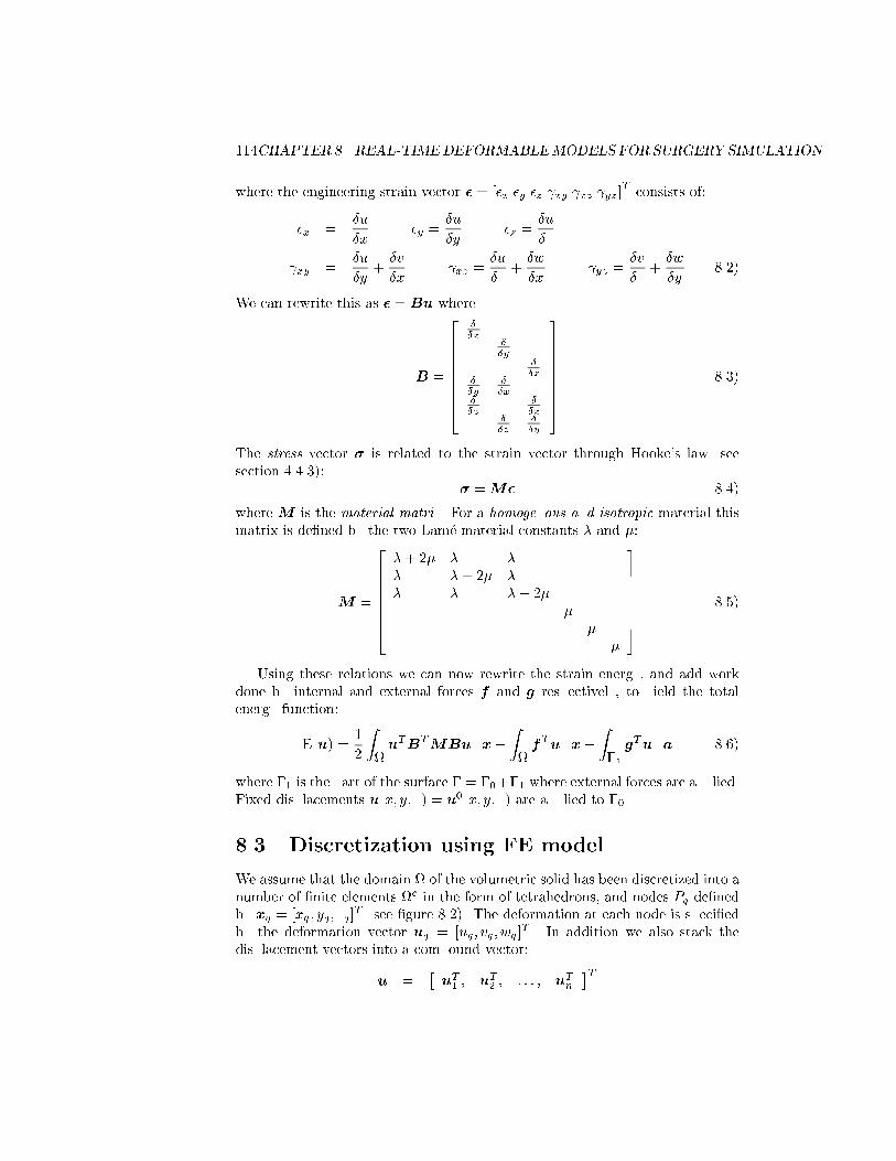
114CHAPTER 8. REAL-TIMEDEFORMABLEMODELS FOR SURGERY SIMULATION
where the engineering strain vector = [x y z xy xz yz]T consists of:
x =u
xy =
u
yz =
u
z
xy =u
y+v
x xz =
u
z+w
x yz =
v
z+w
y(8.2)
We can rewrite this as = Bu where
B =
266666664
x
0 00
y0
0 0 z
y
x
0z
0 x
0 z
y
377777775
(8.3)
The stress vector is related to the strain vector through Hooke's law (seesection 4.4.3):
=M (8.4)
where M is the material matrix. For a homogenous and isotropic material thismatrix is dened by the two Lame material constants and :
M =
26666664
+ 2 0 0 0 + 2 0 0 0 + 2 0 0 00 0 0 0 00 0 0 0 00 0 0 0 0
37777775
(8.5)
Using these relations we can now rewrite the strain energy, and add workdone by internal and external forces f and g respectively, to yield the totalenergy function:
E(u) =1
2
ZuTBTMBu dx
ZfTu dx
Z1
gTu da (8.6)
where 1 is the part of the surface = 0+1 where external forces are applied.Fixed displacements u(x; y; z) = u0(x; y; z) are applied to 0.
8.3 Discretization using FE model
We assume that the domain of the volumetric solid has been discretized into anumber of nite elements e in the form of tetrahedrons, and nodes Pq denedby xq = [xq ; yq; zq]
T (see gure 8.2). The deformation at each node is speciedby the deformation vector uq = [uq; vq ; wq ]
T . In addition we also stack thedisplacement vectors into a compound vector:
u
=uT1 ; uT2 ; : : : ; uTn
T

8.3. DISCRETIZATION USING FE MODEL 115
. . .
. . .. . .
. . .. . .
. . .
Ω
Ω
Ω
ΩΩ
Ω
2
1
3
4N-1
NεΩ
3
4
2
1
e
e
e
e
P
P
P
P
Figure 8.2: Left: Discretization of the domain into nite elements (2D illustra-tion) Right: Tetrahedral nite element.
The nodes of each nite element e are denoted P ei , where i is the local number
of the node, which is unrelated to the global numbering of the nodes. Thediscretized element factors are denoted with a superscripted e. The compoundelement displacement vector is:
ue =
ue1
T ; ue2T ; ue3
T ; ue4TT
(8.7)
As nite elements, four-node tetrahedrons are used with linear interpolationof the displacement eld between the nodes:
u(x) =
4Xi=1
Nei (x)u
ei (8.8)
The basis functions Nei (x) are dened as the natural coordinates Li of the
tetrahedron:
Nei (x) = Li =
1
6V e(aei + beix+ cei y + dei z); i = 1; 2; 3; 4 (8.9)
The natural coordinates, the volume V e and the coecients aei ; bei ; c
ei ; d
ei are all
dened in appendix C.
Using the fact that:
@u
@x=
4Xi=1
@Nei (x)
@xuei (8.10)
@u
@y=
4Xi=1
@Nei (x)
@yuei
@u
@z=
4Xi=1
@Nei (x)
@zuei

116CHAPTER 8. REAL-TIMEDEFORMABLEMODELS FOR SURGERY SIMULATION
where
@Nei (x)=@x =
bei6V e
(8.11)
@Nei (x)=@y =
cei6V e
@Nei (x)=@z =
dei6V e
the discretized strain energy may be written as:
Estrain(u) =
1
2
Xe
Ze
ueTBeTMBeu
edx (8.12)
where Be is dened in appendix C.The solution to the deformation problem is found when the total energy of
the system assumes its minimum value. This happens when the rst variationof the functional E vanishes, ie. when E(u) = 0.
The equilibrium equation E(u) = 0 can be split into element contributions:
E(u) =Xe
Ee(u) = 0 (8.13)
where
Ee(u) =
4Xi=1
@Ee
@ueiuei +
4Xi=1
@Ee
@veivei +
4Xi=1
@Ee
@wei
wei (8.14)
But since the uei , vei and we
i are independent this means that
@Ee
@uei=
@Ee
@vei=
@Ee
@wei
= 0; i = 1; 2; 3; 4 (8.15)
The resulting equilibrium equation for each element thus becomes:
o =
Ze
BeTMBeuedx f
e (8.16)
where f
e is a generalized discretized element compound force vector 1.Because everything inside the integration sign is constant, the equilibrium
equation for the nite element becomes a linear matrix equation:
Keue = f
e (8.17)
whereKe = BeTMBeV e (8.18)
is called the stiness matrix 2 and V e is the volume of the tetrahedron (seeappendix C).
1ue is 12 1, f
e is 12 1 and Be is 6 12
2Ke is 12 12
8.4. SIMPLIFYING THE SYSTEM USING CONDENSATION 117
The only remaining step is assembly of the global stiness matrix and forcevector from the element stiness matrices and force vectors:
K =Xe
global(Ke) (8.19)
f
=Xe
global(f
e)
global() is a transfer function from element node numbers to global node num-bers. The result is a large sparse linear system Ku
= f
.
8.3.1 Fixing nodes
Fixing nodes means clamping them to a xed position, as a tree is clamped tothe ground at the base. If no nodes are clamped it is impossible to solve thelinear system Ku
= f
because K is singular. At least 3 nodes must be xed
for the system to be well-formed.When nodes are assigned a xed displacement, it changes the stiness matrix
K. This change can be applied both on the element stiness matrices and theglobal stiness matrix. Only the approach for the global matrix is shown here,but the same procedure can be applied directly to the element matrices.
Without loss of generality let us assume that the displacement of the lastnode PN is to be xed as uN = u0N = [u0N v0N w0
N ]T . Since the procedure can
be seen as three identical operations modifying rows/columns 3N 2, 3N 1and 3N of the linear system, only the modication of last row/column 3N isdescribed. The modied linear system becomes:2
6664k1;1 : : : k1;3N1 0...
......
...k3N1;1 : : : k3N1;3N1 00 : : : 0 1
37775u
=
26664
f1 w0Nk1;3N
...f3N1 w0
Nk3N1;3Nw0N
37775 (8.20)
The stiness matrix is modied by setting the columns and rows correspondingto the elements of node N to zero with ones in the diagonal. The force vectoris modied to re ect the xed displacement of node N .
8.4 Simplifying the system using condensation
The linear matrix system Ku= f
models the behaviour of the volumetric ob-
ject. This includes both surface nodes as well as the internal nodes of the model.
118CHAPTER 8. REAL-TIMEDEFORMABLEMODELS FOR SURGERY SIMULATION
But for simulation purposes we are usually only interested in the behaviour ofthe surface nodes since these are the only visible nodes.
Fortunately, it is possible to remove the internal nodes from the matrix equa-tion using a technique called condensation [Kar87]. The matrix equation for thecondensed problem has the same size as would result from a FE surface model.But, it is important to understand that it shows exactly the same behaviour forthe surface nodes as the original volumetric system.
Let us assume that the nodes of the FE model have been ordered with thesurface nodes rst, followed by the internal nodes. Using this ordering the linearsystem can be rewritten as a block matrix system (surface / internal):
Kss Ksi
Kis Kii
usu i
=
fsf i
(8.21)
From this block matrix system a new linear matrix system may be derived,which only involves the variables of the surface nodes:
Kssus
= fs
(8.22)
where
Kss = Kss KsiK1ii Kis (8.23)
fs
= fsKsiK
1ii f
i
The displacement of the internal nodes can still be calculated using:
u i
=K1ii (f
iKisu
s) (8.24)
Note, that if no forces are applied to internal nodes, fs
= fs.
Generally the new stiness matrix will be dense compared to the sparsestructure of the original system. But, since the system is to be solved by invert-ing the stiness matrix in the pre-calculation stage, this is not important.
8.5 Solving the linear matrix system
Implicit solution of a linear system is often performed using iterated algorithmssuch as the Conjugate Gradient (CG) [Brt95]. This algorithm performs a sparsematrix vector multiplication, three vector updates and two inner products re-peatedly in an iterative loop. The complexity can therefore roughly be seen asntMv+3v+2vv , where tMv+3v+2vv is the time required for the operations in oneiteration and n is the number of iterations. n is seldom less than 5-10 and can-not in practice be predicted. Especially for a system where the response mustcome at specic frame rates, unpredictable solution time is very unfortunate.
The alternative, which is used here, is to explicitly invert the stiness matrix.Normally this is never done when linear systems resulting from FE models aresolved. The precision of the result suers from numerical errors, and the amount
8.6. SIMULATION 119
of storage needed to store a dense inverted stiness matrix is huge, comparedto the sparse stiness matrix itself. But, as indicated in the beginning of thechapter, precision and memory size are not important when compared withspeed in a trade-o.
Although the time for inversion is considerable, the solution time is verysmall, since it only involves a dense matrix vector multiplication:
u=K1f
(8.25)
Numerical tests have been performed using the Meschach library [Ste92] to solvea linear system generated by a FE model. These experiments included explicitinversion, CG with and without preconditioner, Gauss elimination and severalfactorization techniques such as QR and Cholesky. When the pre-calculationtime was ignored, solution by matrix vector multiplication with the invertedstiness matrix, was at least 10 times faster than any other method.
We have not stated the actual numerical results here, since the implementa-tion of the dierent algorithms in the Meschach library has not been properlyoptimized. The timings could therefore be dierent for other implementations,although the general result would be the same.
8.6 Simulation
In this section we will discuss the dierent simulation methods available to us.We have two linear matrix equations. One with all the nodes of the FE modeland a sparse stiness matrix. And a reduced version with only the surface nodesand a dense stiness matrix.
8.6.1 Dynamic system
In order to use a physically correct model of the body, mass and damping areadded to the static model. This is done by formulating the equation for dampedharmonic motion (discrete version of equation 4.58):
Ru+C _u
+Ku
= f
(8.26)
where R is the mass, C is the damping and K is the stiness matrix of thesystem. K is calculated as shown above. Assuming lumped masses at the nodes,we use diagonal damping and mass element matrices:
Reii =
1
3V e Ce
ii = Reii (8.27)
where is the mass-density and is a scaling factor.The global element matrices are assembled into global matrices. Since the
mass and damping matrices are diagonal, they are also block diagonal. Thedamped harmonic motion equation for the reduced system, therefore, simplybecomes:
Rss us
+Css _us
+ Kssus
= fss
(8.28)

120CHAPTER 8. REAL-TIMEDEFORMABLEMODELS FOR SURGERY SIMULATION
Time discretization
To discretize the time derivatives, nite dierence estimates are used. A semi-implicit Euler method is derived using:
R
t2[u(t+t) 2u
(t) + u
(tt)]
+C
2t[u(t+t) u
(tt)] +Ku
(t+t) = f
(t) (8.29)
or Ku(t+t) = f
(t) where:
K =R
t2+
C
2t+K
f(t) =
2R
t2u(t) +
C
2t R
t2
u(tt) + f
(t) (8.30)
The equations for a comparable explicit solution are:
R
t2[u(t+t) 2u
(t) + u
(tt)]
+C
2t[u(t+t) u
(tt)] +Ku
(t) = f
(t) (8.31)
or
u(t+t) =
R
t2+
C
2t
1
2R
t2u(t)
R
t2 C
2t
u(tt)
Ku(t) + f
(t)
(8.32)
Since both R and C are diagonal matrices, they are easily inverted.The main feature of the explicit solution method is that the stiness matrix
K does not have to be inverted. In practice, this allows us to split the largeglobal equation into simple independent local equations for each node:
uq(t+t) =
V e
3t2+V e
6t
1
2V e
3t2uq(t)
V e
3t2 V e
6t
uq(tt))
fKu(t)gq + fq(t)
=
1
t+
2
1
2
tuq(t)
1
t
2
uq(tt))
3t
V e
fKu(t)gq + fq(t)
(8.33)
8.6. SIMULATION 121
where fKu(t)gq is the result of the matrix-vector multiplication related to the
node q.
Simulation using this equation would be similar to the mass-spring mod-els used by eg. Kuhnapfel, Deussen, and Kuhn [Deu95, Ku96, Kue93, Kue94,Kue95] and Waters and Terzopoulos [Wat87, Wat91, Ter91b, Wat92, Ter93,Lee93, Lee95].
The non-zero elements of the row associated with the q'th node of K, indi-cate which nodes that are connected to it with springs.
The semi-implicit solution algorithm is preferred because of the better sta-bility and more direct solution of the system. System response is more globalwith the implicit approach. Using explicit methods, the response to forces isonly spread globally after some iterations.
A drawback with the semi-implicit models is the greater diculty of model-ing cuts. Any change in the stiness matrix implies that the inverted stinessmatrix has to be updates or recalculated. This can be quite expensive. Butwith domain decomposition techniques, the domain may be split up into sub-domains, which use explicit and semi-implict solution methods, depending onwhether cuts have been or have not been performed in the sub-domain. See thelater section 8.9.1 for a wider discussion of these aspects.
Although the discussion above has been carried out using the full system,the same equations could be formulated for the condensed system. We leavethis to the reader.
8.6.2 Static system and selective matrix vector multipli-
cation
Generally the f(t) vector is a full vector because of the contribution from the
previous displacement vectors u(t) and u
(tt). In contrast the original force
vector f(t) is a sparse vector when forces only are applied to a few surface
nodes. Since this is often the case in simulation, we were inspired to develop analternative simulation method, which for sparse force vectors, is considerablyfaster.
The cost of this simulation method is the loss of dynamics. The idea is touse the static linear system Ku
= f
(or the condensed version) instead of the
dynamic damped harmonic motion system, and exploit the sparse structure ofthe static force vector.
Formally, solving the system using the inverted stiness matrix is performedusing:
u=K1f
(8.34)
If only a few positions of the force vector are non-zero, clearly standard matrixvector multiplication would involve a large number of super uous multiplica-tions. Note that:
u=K1f
=Xi
K1i fi
(8.35)

122CHAPTER 8. REAL-TIMEDEFORMABLEMODELS FOR SURGERY SIMULATION
whereK1i is the i'th column vector ofK1 and fi
the i'th element of f
. Since
the majority of the fiare zero, i is restricted to run through only the positions of
ffor which fi
6= 0. If n of the N positions in f
are non-zero this will reduce the
complexity to O(n=N) times the time of a normal matrix vector multiplication.We call this approach Selective Matrix Vector Multiplication (SMVM).
The SMVM method and the dynamic model converge for slow changes inforces applied to the solid body.
8.6.3 Summary of simulation methods
A number of methods related to simulation using FE models have been pre-sented. In general two criterias separate the possible implicit algorithms: FullFE model contra condensed FE model, and dynamic simulation contra selectivematrix vector multiplication (SMVM).
Dynamic simulation SMVM
Full FE model FD FSCondensed FE model CD CS
The choice of algorithm depends on the requirements of the application. Whetherone chooses dynamic simulation or SMVM is a question of the speed require-ment and size of the problem. If the problem can be processed fast enough usingdynamic simulation, this would be the best choice.
The choice between the full FE model versus the condensed model, is basedon whether it is necessary to modify the FE model during simulation or not, eg.to model a surgical cut in the model. If modication is necessary, the standardfull system is easier to modify, rather than the condensed system, which is onestep further in renement. Without the need for modication the condensedmodel should be used.
The CS, CD and FS methods have been implemented in the simulationsystem described below.
8.7 Simulation system
This section brie y discusses the practical aspects of implementing the simu-lation methods and generating models from voxel data. Screen shots from theSGI Performer based system are used to illustrate the results.
8.7.1 Mesh generation using Mvox and Nuages
In addition to a range of simple box-like structures, data from the Visible Humanproject [Vis96] has been used to make a model of a lower leg.
Since the Visible Human data set is voxel-based (see gure 8.3), it mustrst be turned into a mesh model. The Mvox software [BN96] is used to drawcontours manually on the boundary of the skin and bone in the voxel data(see gure 8.4). The Nuages software [Gei93] is then applied to create a 3D

8.7. SIMULATION SYSTEM 123
Figure 8.3: Voxel data from the visible human data set.
tetrahedral mesh model of the leg. The result for the lower leg is shown ingure 8.5. This model is used in the simulation system described in the nextsection.
8.7.2 SGI Performer parallel pipe-lining system
The simulation system has been implemented on a Silicon Graphics Onyx withfour Mips R4400 processors using the SGI Performer 1.2 graphics library. SGIPerformer allows the programmer to create parallel pipe-lining software quiteeasily by providing the basic tools for communication, shared memory etc.
Currently, the system runs with 3 processes (see gure 8.7): The Application,Culling and Drawing processes. The Application process handles the actualsimulation of the deformable solid, ie. calculates displacements etc. The Cullingprocess analyzes the scene that the simulation process provides, and determineswhich parts are visible in the current window. It then pipes the visible parts tothe Drawing process which nally renders the scene.
Note, that although the entire system is a parallel system, the actual defor-mation simulation system still runs on a single processor. The parallel featuresare only used to separate rendering from simulation.
Figure 8.6 shows a screen dump of the virtual surgery room with the leglying on the operating table. Figure 8.8 shows the surface of the FE mesh inthe simulator.
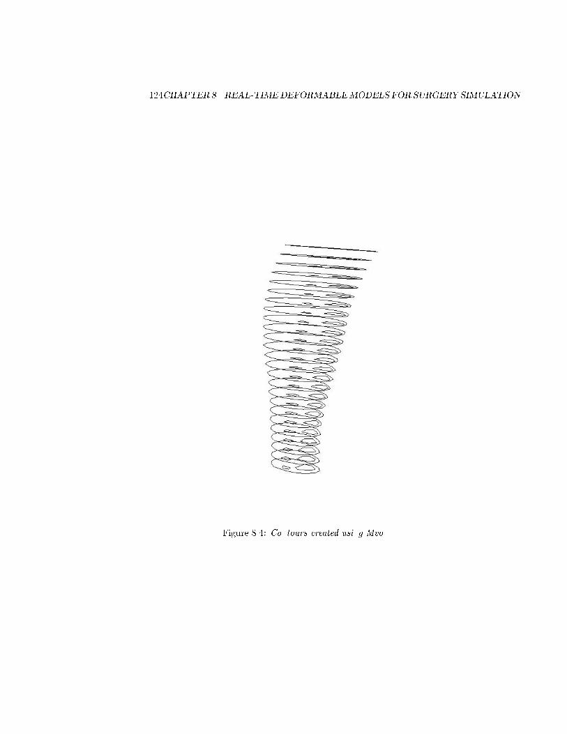
124CHAPTER 8. REAL-TIMEDEFORMABLEMODELS FOR SURGERY SIMULATION
Figure 8.4: Contours created using Mvox.

8.7. SIMULATION SYSTEM 125
Figure 8.5: FE mesh created from contours using Nuages.
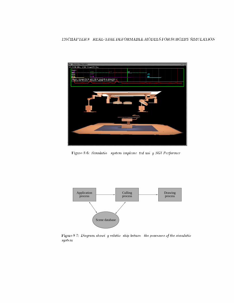
126CHAPTER 8. REAL-TIMEDEFORMABLEMODELS FOR SURGERY SIMULATION
Figure 8.6: Simulation system implemented using SGI Performer.
DrawingCullingApplicationprocess process process
Scene database
Figure 8.7: Diagram showing relationship between the processes of the simulationsystem.
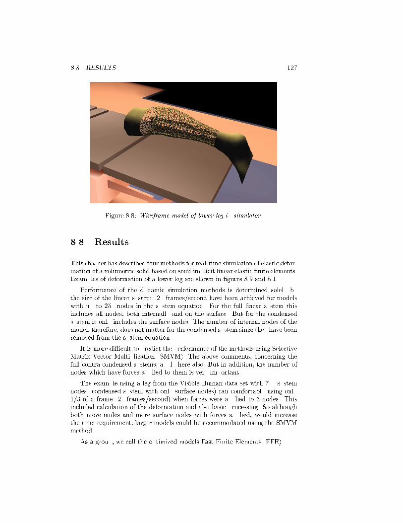
8.8. RESULTS 127
Figure 8.8: Wireframe model of lower leg in simulator.
8.8 Results
This chapter has described four methods for real-time simulation of elastic defor-mation of a volumetric solid based on semi-implicit linear elastic nite elements.Examples of deformation of a lower leg are shown in gures 8.9 and 8.10.
Performance of the dynamic simulation methods is determined solely bythe size of the linear system. 20 frames/second have been achieved for modelswith up to 250 nodes in the system equation. For the full linear system thisincludes all nodes, both internally and on the surface. But for the condensedsystem it only includes the surface nodes. The number of internal nodes of themodel, therefore, does not matter for the condensed system since they have beenremoved from the system equation.
It is more dicult to predict the performance of the methods using SelectiveMatrix Vector Multiplication (SMVM). The above comments, concerning thefull contra condensed systems, apply here also. But in addition, the number ofnodes which have forces applied to them is very important.
The example using a leg from the Visible Human data set with 700 systemnodes (condensed system with only surface nodes) ran comfortably using only1/3 of a frame (20 frames/second) when forces were applied to 3 nodes. Thisincluded calculation of the deformation and also basic processing. So althoughboth more nodes and more surface nodes with forces applied, would increasethe time requirement, larger models could be accommodated using the SMVMmethod.
As a group, we call the optimized models Fast Finite Elements (FFE).
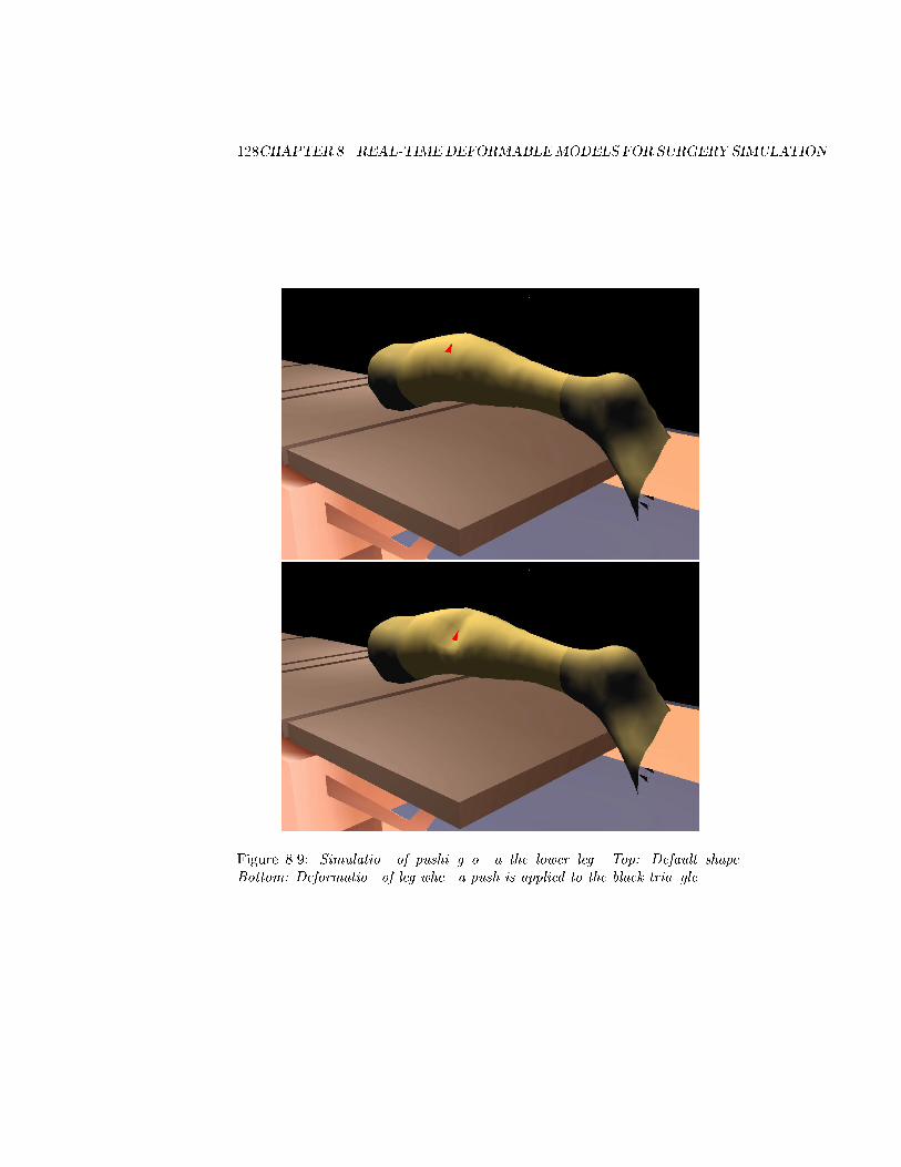
128CHAPTER 8. REAL-TIMEDEFORMABLEMODELS FOR SURGERY SIMULATION
Figure 8.9: Simulation of pushing on a the lower leg. Top: Default shape.Bottom: Deformation of leg when a push is applied to the black triangle.

8.8. RESULTS 129
Figure 8.10: Simulation of pulling on a the lower leg. Top: Default shape.Bottom: Deformation of leg when a push is applied to the black triangle.
130CHAPTER 8. REAL-TIMEDEFORMABLEMODELS FOR SURGERY SIMULATION
8.9 Extensions
This section describes two extensions to the basic fast nite element algorithms,which could be used in larger practical systems. Full implementation of theseextensions requires considerable database handling facilities, and access to par-allel systems with at least 5-10 processors.
8.9.1 Domain decomposition
The computational complexity of the nite element models is generally high.Although computational improvements have been presented in this chapter,there is still a low limit on the possible size of the deformable models, if real-time response is necessary.
Parallel processors are starting to become generally available on eg. the Sili-con Graphics Onyx series of high-end graphics computers. A natural suggestionis, therefore, to create parallel versions of the nite element models.
Explicit models are very easy to parallelize, since the solution is determinedlocally. In principle, each node can therefore be assigned to one processor in theparallel computer.
Creating parallel versions of implicit models is more dicult. Fortunately,there is currently a great deal of attention on these problems. Domain decom-position techniques are being developed with the specic aim of implementingnite element models on parallel systems. Although the eld is still being de-veloped, there are reasonable methods available.
In the following, the basic ideas of domain decomposition are described.Domain decomposition methods can be quite complex, and it is not clear whichmethod should be used for the real-time deformable models. A more detaileddescription is, therefore, not given here. Refer to the recent book by Smith etal. [Smi96] for a more in-depth discussion.
Let us assume that the domain can be separated into non-overlappingsub-domains (i) with boundaries (i) (see gure 8.11). Adjacent domains i
and j only share the common boundary (i) \ (j).Let the linear system for sub-domain i be:
K(i)u(i) = f
(i) (8.36)
Using the same approach as used for the condensation, the nodes of the sub-domain are split into interior and common nodes. The common nodes are thoseshared by two or more sub-domains.
With these denitions, the equilibrium matrix equation for the sub-domaincan be written as: "
K(i)cc K
(i)ci
K(i)ic K
(i)ii
#"u(i)c
u(i)i
#=
"f
(i)
c
f
(i)
i
#(8.37)
From this block matrix system a new linear matrix system may be derived,

8.9. EXTENSIONS 131
(4)Ω
Ω(2)
Ω(3)
(1)Ω
(3) (4)
(2)Γ(1) Γ
ΓΓ
Figure 8.11: Domain decomposition.
which only involves the variables of the common nodes:
K(i)
cc u(i)c = f
(i)
c(8.38)
where
K(i)
cc = K(i)cc K(i)
ci K(i)1ii K
(i)ic (8.39)
f
(i)
c= f
(i)
cK(i)
ci K(i)1ii f
(i)
i(8.40)
The sub-domain variables are assembled into a global system
Kccuc
= fc
(8.41)
where Kcc is called the Schur's complement.Finally, when a solution has been found for the common nodes, the displace-
ments of the internal nodes in the sub-domain can be calculated using:
u(i)i =K
(i)1ii (f
(i)
iK(i)
ic u(i)c ) (8.42)
In theory, the following approach could be used to solve the global matrixequation using domain decomposition (Parallel indicates that the step can becarried out in parallel):
1. Parallel: The common forces are determined locally in each sub-domainusing equation 8.40,
2. These forces are assembled into a global force vector, which is used to ndthe displacements of the common nodes using equation 8.41,
132CHAPTER 8. REAL-TIMEDEFORMABLEMODELS FOR SURGERY SIMULATION
3. Parallel: When the displacements of the common nodes are found, thedisplacements of the internal nodes can be determined using equation 8.42.
Normal domain decomposition methods do not use this approach directly. In-stead iterated conjugate gradient methods [Brt95] are often used with precon-ditioners based on the Schur's complement.
The actual application will determine what form of domain decompositionalgorithm should be used. In the case of cutting, the Schur's complements arechanged and iterated methods are probably necessary.
Experiments have been carried out to solve the global linear system:
Ku= f
(8.43)
by applying domain decomposition based on the conjugate gradient algorithm.
First a preconditioner is created from the global stiness matrix by zeroingthe o-diagonal elements, which are related to the common nodes. Since thesub-domain blocks of the preconditioner are now independent, the applicationof the preconditioner in the conjugate gradient algorithm, can be carried out inparallel by sub-domain processors. The remaining part of the conjugate gradientalgorithm is global, and can be performed on a specially assigned processor.
Preliminary results have been obtained showing the validity of the algorithm.But, the conjugate gradient algorithm is slow, and the solution of the globalsystem was not fast enough for real-time performance. More work is thereforenecessary, to determine an appropriate domain decomposition algorithm.
8.9.2 Cutting in nite element systems
Implementing cutting in nite element systems causes two major problems. Therst, which we ignore here, is related to the geometric modication of the niteelement mesh. These modications should ensure that the cut looks smoothwhen rendered using computer graphics. In general, it is necessary to rene themesh around the cut, and the geometric aspects of this are non-trivial.
The second problem concerns the necessary change of the stiness matrixand the linear system. For explicit methods this is simple. But, for implicitsystems, where the stiness matrix has been inverted, the inverted stinessmatrix needs to be updated.
For simplicity, let us assume that the cutting implies removing the niteelement number e from the system. The modied stiness matrix becomes:
K =K global(Ke) (8.44)
Since the size of the element stiness matrix is 12 12, this involves changes in12 rows and 12 columns.
To change the inverted stiness matrix, the Woodbury formula [Num92]is used. The Woodbury formula is a matrix extension of the original scalarSherman-Morrison update formula.
8.10. SUMMARY 133
Let us assume that the stiness matrix is updated with a matrix, which canbe written as the outer product of two 3N 12 vectors (N is the number ofnodes):
K !K +UV T (8.45)
The updated inverted stiness matrix then becomes:
(K +UV T )1 = K1 (8.46)
hK1U (I1212 + V
TK1U )1V TK1i
(8.47)
where I1212 is a 12 by 12 identity matrix.The vectors U and V are easily determined: Ke and the identity matrix
are inserted in the rows of U and V , respectively, corresponding to the globalrow/column positions of the element nodes.
The computation consists of the inversion of the 12 by 12 matrix:
I1212 + VTK1U (8.48)
and 6 matrix multiplications of dierent sizes and two matrix additions. In total324N2 +O(N) ops.
To demonstrate the applicability of this approach, a simple cutting algo-rithm has been implemented in the simulation system. This algorithm allowsindividual nite elements to be removed. The resulting modication of thelinear system is obtained using the algorithm described above.
An example is shown in gure 8.12. This simple nite element model has only75 nodes and the modication of the linear system is more or less instant. For amore complex mesh with 1125 nodes, the modication of the inverted stinessmatrix takes about one minute. The time consumption is, consequently, toohigh for general real-time response. But, it could be used in specic cases,where the waiting time can be accepted or otherwise disguised.
8.10 Summary
In this chapter, a comprehensive description of the issues facing a developer ofreal-time deformable models has been given. In particular, new results usingcondensation techniques, direct matrix inversion, and selective matrix vectormultiplication were presented. These methods are essential to obtaining accept-able response in surgery simulation systems.
A simulation system developed using SGI Performer was described, and aroutine for creating the basic nite element mesh was suggested.
Two important extensions of the work were outlined in the nal section.These extensions are the use of domain decomposition for parallel implemen-tation of the nite element system, and the procedure for modication of thesystem matrix in response to cuts in the mesh.
A simple example of a cut were demonstrated, in which a single nite elementwas removed from the stiness matrix and a hole appeared.

134CHAPTER 8. REAL-TIMEDEFORMABLEMODELS FOR SURGERY SIMULATION
Figure 8.12: Simple cutting in nite element mesh.

8.10. SUMMARY 135
The implementations of the two extensions are non-trivial and require com-prehensive book-keeping and computer power to work in practice. Both exten-sions, consequently, need more work before they can be used in practice.
In general, there is still a considerable amount of work to be performed. Animportant example is the introduction of detailed segmentations of the organs,limbs etc. to allow dierent material properties and models to be used. Thecurrent parallel research in digital atlasses such as the VoxelMan atlas [Hoe92]is a signicant step in this direction.

136CHAPTER 8. REAL-TIMEDEFORMABLEMODELS FOR SURGERY SIMULATION
Chapter 9
Conclusion
In this thesis, medical image registration and surgery simulation techniques havebeen explored. Reviews of previous work in these elds were given in chapters 2and 7.
If rigid transformation is understood as physical motion, physical modelshas been the common denominator of all the work presented here.
In general, physical models are becoming more and more important in theelds of image processing, computer graphics, medical imaging, and simulation.This is happening, because in all these elds there is a movement in these years,from regarding the world as consisting of rigid objects, to taking the naturalpath of regarding the world as simply - the world.
The environment is, therefore, increasingly being simulated and interpre-tated using non-rigid modeling techniques, which have their basis in physicalmodels of natural phenomena.
Often the physical models have been used without regard to their actualapplicability for the specic problem. This is natural when new techniques areintroduced to a eld, but unfortunate in the long run, since problems inevitablyoccur. This text has, therefore, been written with a strong emphasis on reallyunderstanding the physical models and their limitations. In particular, chapter 4were dedicated to a in-depth description of physical continuum models.
Some of the results in this thesis have come about because this understandingopened up new ways of handling the specic problems. This was seen in chap-ter 5, where the viscous uid registration algorithm were improved using resultsfrom linear elasticity. This transfer of knowledge from one model to another,was made possible by a general understanding of continuum models.
In addition, the implementation of the linear elasticity operator as a l-ter, depended on an understanding of the characteristics of quadratic energyfunctions, and their linear partial dierential equations.
Sometimes, it is not possible to use the appropriate physical model becauseof computational complexity considerations. The real-time nite element mod-els of linear elasticity in chapter 8 are a good example of a case where a modelis selected entirely based on timing concerns. But, although the specic appli-
137
138 CHAPTER 9. CONCLUSION
cation without doubt violates basic assumptions of the model, the knowledge ofthe continuum models allows us to understand when and how these assumptionsare violated. Thus, we are able to make an intelligent trade-o, rather than ablind decision.
In some cases, the real physical model is not known. Naturally, this hampersthe use of realistic models, and often an arbitrary model is used instead. Thishas typicly happened for non-rigid registration of medical images. Since nomodel of the change from one image to the next is generally available, elasticand viscous uid models have been used instead.
But, in isolated cases it is possible to determine the real physical model.Chapter 6 described such a case, where theories about the real model were usedto build a specic model for the problem at hand. In this chapter, time sequenceimages of the mandibular bone were registered using a growth model, based onmedical knowledge of the growth processes of bone.
Finally, there are alternative aspects to this thesis than the physical mod-els. Physical models have been the theoretical hinge of thesis. But, the thesiscan also be seen from an application point of view. Indeed, as argued in theintroduction, the image registration and simulation algorithms presented here,can be seen as some of the basic elements of the next generation medical work-station. A workstation, where all the components of visualization, automateddiagnosis, surgery simulation, and surgery assistance, come together.
Whether this workstation will ever see the light is another question. Thereis still a long way to go, and this thesis has only solved a small part of theproblems. Much of the next generation workstation is still visions of the futureof medicine.
There is a lot of work in front of us.
Appendix A
Mvox
Mvox is a general-purpose tool for visualization, segmentation and manipulationof a wide range of 2-4D greylevel and color images, and 3D surface graphics.The software provides a exible tool, that handles all the data types typicallyused in a research environment, for medical imaging and visualization.
Mvox is easy to use, and has a consistent user interface, based on softwarestandards such as Unix, X/Motif and OpenGL.
Mvox can handle images with dierent numbers of slices, colors, and timesteps. It has been successfully used to visualize and segment:
2D and 3D medical images with stacks of slices (CT, MRI, etc).
2D and 3D color images, such as histological slices from the Visible Humandata set.
2D remote sensing images with many channels,
3D surface graphics, such as those used in CAD software and produced bythe iso-surface routine in Mvox [Wyv86] (similar to Marching Cubes [Lor87]).
time sequences of any of the above.
In Mvox, image segmentation can be performed manually using editing andcontour drawing facilities (see gure A.3). For semi-automatic segmentation,Mvox has interactive/automatic thresholding (see gure A.2) and statisticalclassication using discriminant analysis [Con84], both with multiple classes.
Segmented images can be visualized in 3D, along with the original images,using either iso-surfacing [Wyv86], volume rendering or fast display of slices (seegure A.4 and A.5). Also stacked contours can be turned into 3D structures.
Additional features include image registration, computation and manipula-tion of image histograms, computation of image statistics, colormap alteration,etc. User-developed C programs can use Mvox as a front-end through a sharedmemory interface by including as little as two lines of extra user code. All thismakes Mvox a very exible tool suited to a wide variety of user needs.
Images in this appendix show dierent screen-shots from Mvox.
139
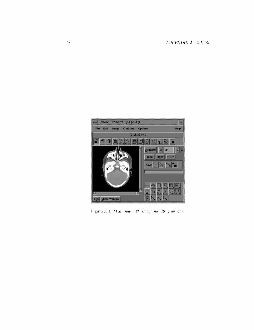
140 APPENDIX A. MVOX
Figure A.1: Mvox main 2D image handling window.
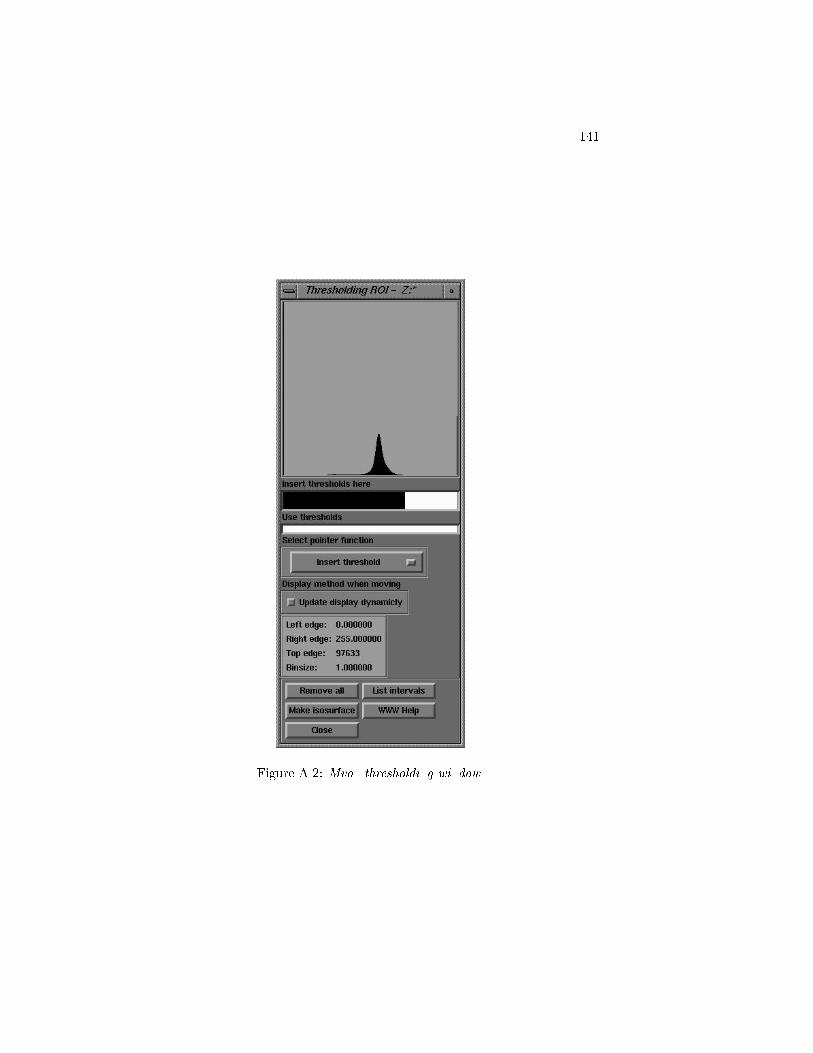
141
Figure A.2: Mvox thresholding window.
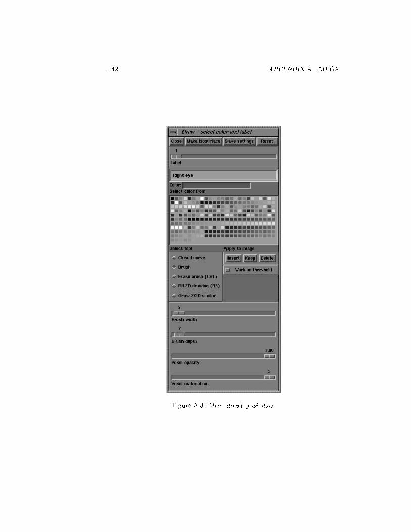
142 APPENDIX A. MVOX
Figure A.3: Mvox drawing window.

143
Figure A.4: Mvox 3D graphics window.
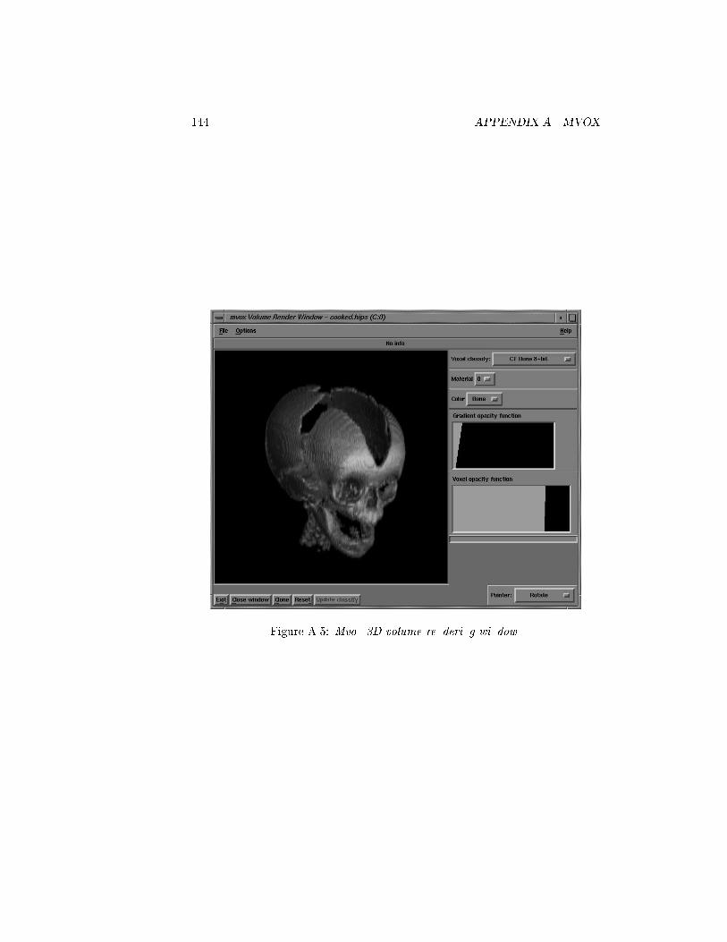
144 APPENDIX A. MVOX
Figure A.5: Mvox 3D volume rendering window.
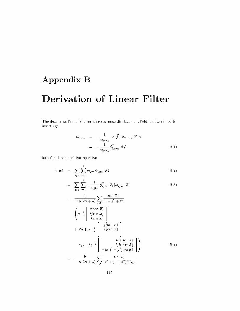
Appendix B
Derivation of Linear Filter.
The decomposition of the impulse response displacement eld is determined byinserting:
lmns = 1
lmns
< ~fc;lmns(~x) >
= 1
lmns
x1lmns(~xc) (B.1)
into the decomposition equation.
~v(~x) =
1Xijk
3Xr=1
ijkrijkr(~x) (B.2)
=
1Xijk
3Xr=1
1
ijkrx1ijkr(~xc)ijkr(~x) (B.3)
=1
2(2+ )
1Xijk
scc(~x)
i2 + j2 + k20@21
24 i2scc(~x)
ijcsc(~x)ikccs(~x)
35
+(2+ )22
24 j2scc(~x)ijcsc(~x)
0
35
+(2+ )23
24 (ik)2scc(~x)
ijk2csc(~x)ik(i2 + j2)ccs(~x)
351A (B.4)
=8
2(2+ )
1Xijk
scc(~x)
(i2 + j2 + k2)2ijk
145
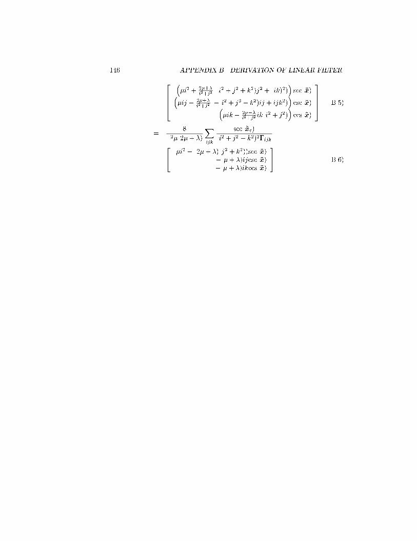
146 APPENDIX B. DERIVATION OF LINEAR FILTER.
26664
i2 + 2+
i2+j2 ((i2 + j2 + k2)j2 + (ik)2)
scc(~x)
ij + 2+i2+j2 ((i2 + j2 + k2)ij + ijk2)
csc(~x)
ik 2+i2+j2 ik(i
2 + j2)ccs(~x)
37775 (B.5)
=8
2(2+ )
1Xijk
scc(~xc)
(i2 + j2 + k2)2ijk24 (i2 + (2+ )(j2 + k2))scc(~x)
(+ )ijcsc(~x)(+ )ikccs(~x)
35 (B.6)
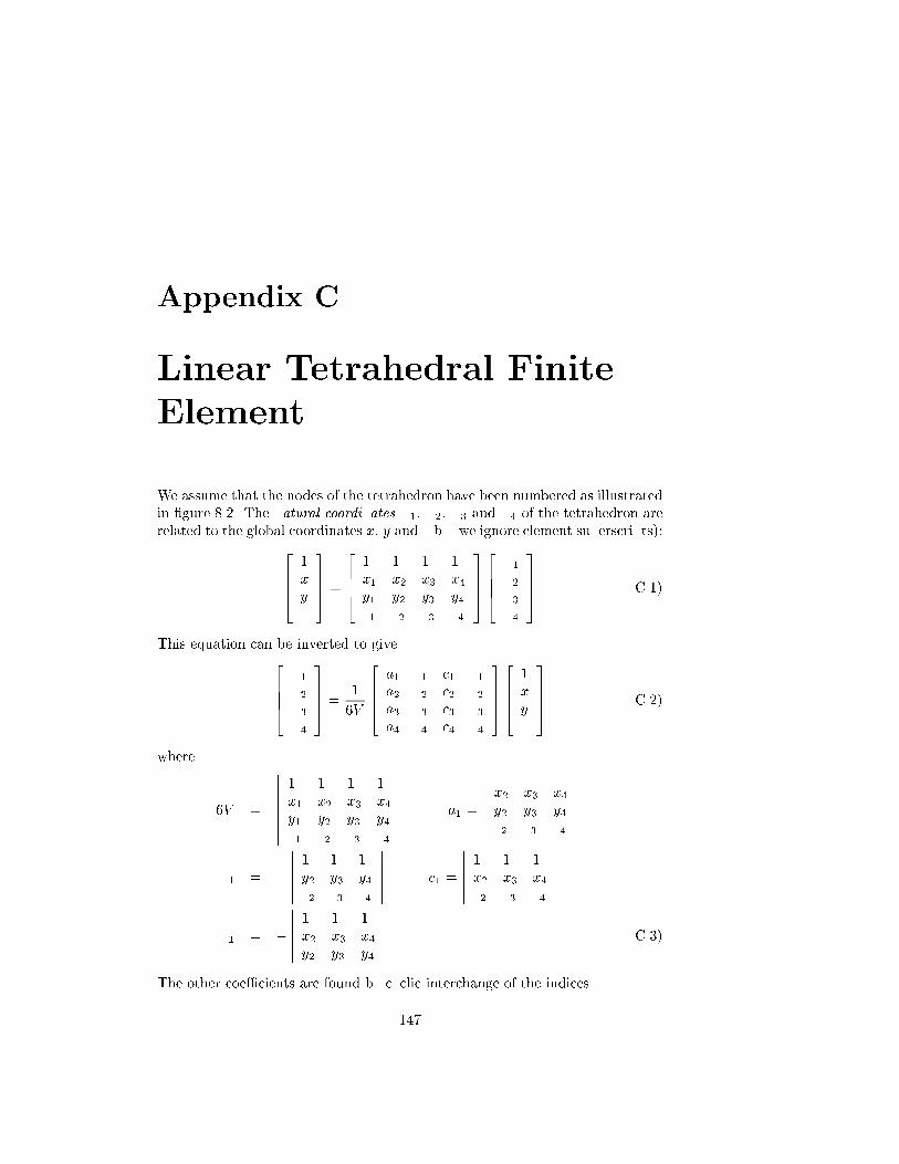
Appendix C
Linear Tetrahedral Finite
Element
We assume that the nodes of the tetrahedron have been numbered as illustratedin gure 8.2. The natural coordinates L1, L2, L3 and L4 of the tetrahedron arerelated to the global coordinates x, y and z by (we ignore element superscripts):2
6641xyz
3775 =
2664
1 1 1 1x1 x2 x3 x4y1 y2 y3 y4z1 z2 z3 z4
37752664
L1
L2
L3
L4
3775 (C.1)
This equation can be inverted to give2664
L1
L2
L3
L4
3775 =
1
6V
2664
a1 b1 c1 d1a2 b2 c2 d2a3 b3 c3 d3a4 b4 c4 d4
37752664
1xyz
3775 (C.2)
where
6V =
1 1 1 1x1 x2 x3 x4y1 y2 y3 y4z1 z2 z3 z4
a1 =
x2 x3 x4y2 y3 y4z2 z3 z4
b1 =
1 1 1y2 y3 y4z2 z3 z4
c1 =
1 1 1x2 x3 x4z2 z3 z4
d1 =
1 1 1x2 x3 x4y2 y3 y4
(C.3)
The other coecients are found by cyclic interchange of the indices.
147
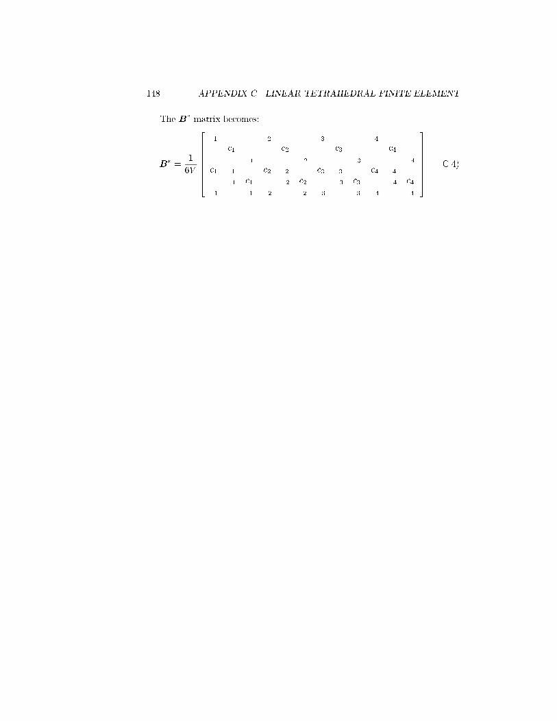
148 APPENDIX C. LINEAR TETRAHEDRAL FINITE ELEMENT
The Be matrix becomes:
Be =1
6V
26666664
b1 0 0 b2 0 0 b3 0 0 b4 0 00 c1 0 0 c2 0 0 c3 0 0 c4 00 0 d1 0 0 d2 0 0 d3 0 0 d4c1 b1 0 c2 b2 0 c3 b3 0 c4 b4 00 d1 c1 0 d2 c2 0 d3 c3 0 d4 c4d1 0 b1 d2 0 b2 d3 0 b3 d4 0 b4
37777775
(C.4)

Appendix D
GLCM Plots
D.1 MR-Pd / MR-T1 (moved)
149
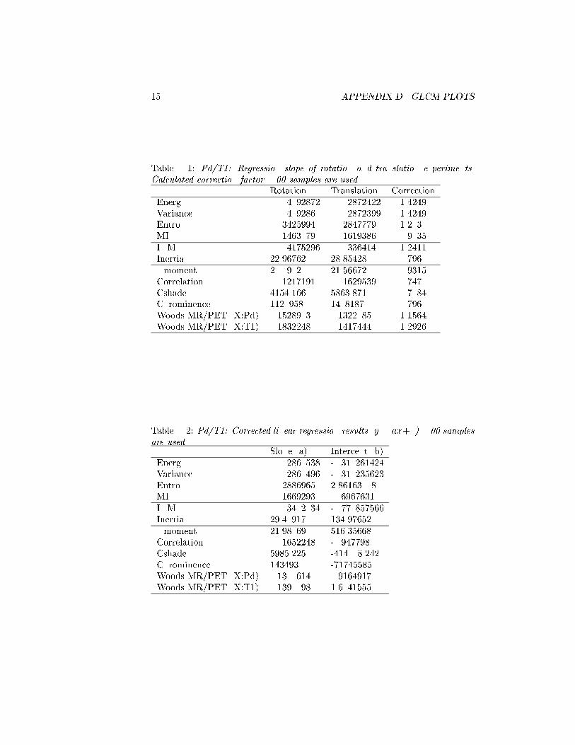
150 APPENDIX D. GLCM PLOTS
Table D.1: Pd/T1: Regression slope of rotation and translation experiments.Calculated correction factor. 500 samples are used.
Rotation Translation CorrectionEnergy 0.004092872 0.002872422 1.4249Variance 0.00409286 0.002872399 1.4249Entropy 0.03425994 0.02847779 1.2030MI 0.01463079 0.01619386 0.9035IDM 0.004175296 0.00336414 1.2411Inertia 22.96762 28.85428 0.7960Dmoment 20.0902 21.56672 0.9315Correlation 0.01217191 0.01629539 0.7470Cshade 4154.166 5863.871 0.7084Cprominence 1120958 1408187 0.7960Woods MR/PET (X:Pd) 0.1528903 0.1322085 1.1564Woods MR/PET (X:T1) 0.1832248 0.1417444 1.2926
Table D.2: Pd/T1: Corrected linear regression results (y = ax+b). 500 samplesare used.
Slope (a) Intercept (b)Energy 0.002860538 -0.310261424Variance 0.002860496 -0.310235623Entropy 0.02886965 2.86163008MI 0.01669293 -0.69676310IDM 0.003402034 -0.770857566Inertia 29.40917 134.97652Dmoment 21.98069 516.35668Correlation 0.01652248 -0.94779800Cshade 5985.225 -414008.242Cprominence 1434930 -71745585Woods MR/PET (X:Pd) 0.1300614 0.9164917Woods MR/PET (X:T1) 0.1390098 1.6041555
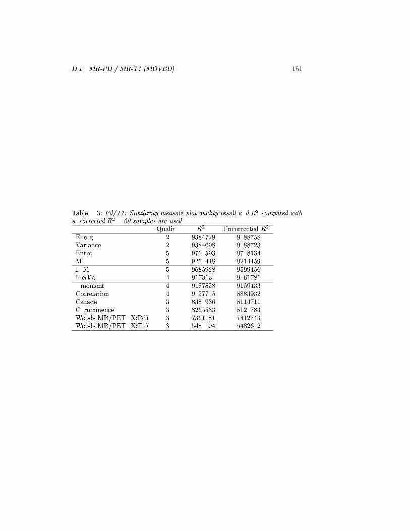
D.1. MR-PD / MR-T1 (MOVED) 151
Table D.3: Pd/T1: Similarity measure plot quality result and R2 compared withuncorrected R2. 500 samples are used.
Quality R2 Uncorrected R2
Energy 2 0.9384729 0.9088758Variance 2 0.9384698 0.9088723Entropy 5 0.9760593 0.9708134MI 5 0.9260448 0.9214459IDM 5 0.9685928 0.9599456Inertia 4 0.9173130 0.9061781Dmoment 4 0.9187858 0.9159433Correlation 4 0.9057705 0.8883932Cshade 3 0.8380936 0.8114711Cprominence 3 0.8265533 0.8120783Woods MR/PET (X:Pd) 3 0.7361181 0.7412743Woods MR/PET (X:T1) 3 0.5480094 0.5482602
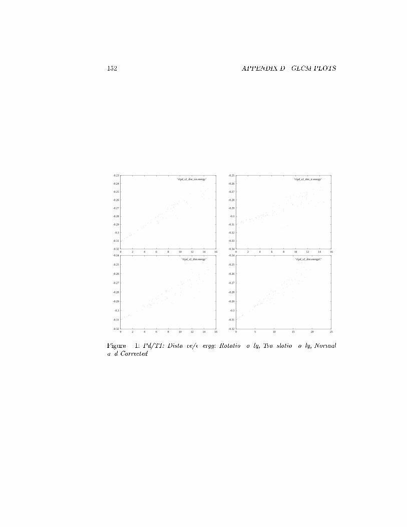
152 APPENDIX D. GLCM PLOTS
-0.32
-0.31
-0.3
-0.29
-0.28
-0.27
-0.26
-0.25
-0.24
-0.23
0 2 4 6 8 10 12 14 16
’t1pd_s2_dist_rot.energy’
-0.34
-0.33
-0.32
-0.31
-0.3
-0.29
-0.28
-0.27
-0.26
-0.25
0 2 4 6 8 10 12 14 16
’t1pd_s2_dist_tr.energy’
-0.32
-0.31
-0.3
-0.29
-0.28
-0.27
-0.26
-0.25
-0.24
0 2 4 6 8 10 12 14 16
’t1pd_s2_dist.energy’
-0.32
-0.31
-0.3
-0.29
-0.28
-0.27
-0.26
-0.25
-0.24
0 5 10 15 20 25
’t1pd_s2_dist.energyC’
Figure D.1: Pd/T1: Distance/energy: Rotation only, Translation only, Normaland Corrected.

D.1. MR-PD / MR-T1 (MOVED) 153
-0.32
-0.31
-0.3
-0.29
-0.28
-0.27
-0.26
-0.25
-0.24
-0.23
0 2 4 6 8 10 12 14 16
’t1pd_s2_dist_rot.variance’
-0.34
-0.33
-0.32
-0.31
-0.3
-0.29
-0.28
-0.27
-0.26
-0.25
0 2 4 6 8 10 12 14 16
’t1pd_s2_dist_tr.variance’
-0.32
-0.31
-0.3
-0.29
-0.28
-0.27
-0.26
-0.25
-0.24
0 2 4 6 8 10 12 14 16
’t1pd_s2_dist.variance’
-0.32
-0.31
-0.3
-0.29
-0.28
-0.27
-0.26
-0.25
-0.24
0 5 10 15 20 25
’t1pd_s2_dist.varianceC’
Figure D.2: Pd/T1: Distance/variance: Rotation only, Translation only, Nor-mal and Corrected.
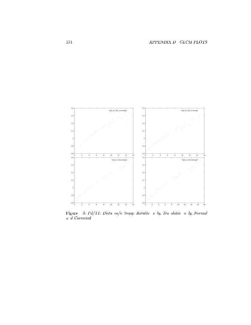
154 APPENDIX D. GLCM PLOTS
2.8
2.9
3
3.1
3.2
3.3
3.4
0 2 4 6 8 10 12 14 16
’t1pd_s2_dist_rot.entropy’
2.8
2.9
3
3.1
3.2
3.3
3.4
0 2 4 6 8 10 12 14 16
’t1pd_s2_dist_tr.entropy’
2.8
2.9
3
3.1
3.2
3.3
3.4
0 2 4 6 8 10 12 14 16
’t1pd_s2_dist.entropy’
2.8
2.9
3
3.1
3.2
3.3
3.4
0 2 4 6 8 10 12 14 16 18
’t1pd_s2_dist.entropyC’
Figure D.3: Pd/T1: Distance/entropy: Rotation only, Translation only, Normaland Corrected.
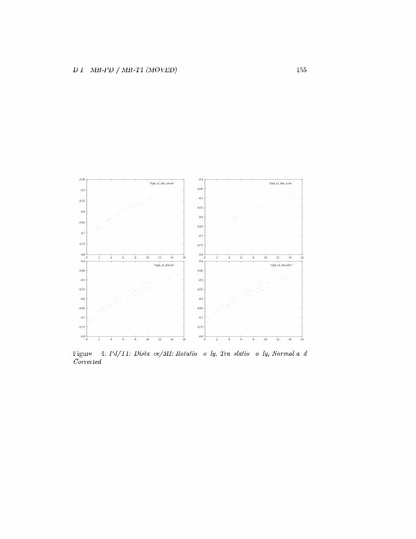
D.1. MR-PD / MR-T1 (MOVED) 155
-0.8
-0.75
-0.7
-0.65
-0.6
-0.55
-0.5
-0.45
0 2 4 6 8 10 12 14 16
’t1pd_s2_dist_rot.mi’
-0.8
-0.75
-0.7
-0.65
-0.6
-0.55
-0.5
-0.45
-0.4
0 2 4 6 8 10 12 14 16
’t1pd_s2_dist_tr.mi’
-0.8
-0.75
-0.7
-0.65
-0.6
-0.55
-0.5
-0.45
-0.4
0 2 4 6 8 10 12 14 16
’t1pd_s2_dist.mi’
-0.8
-0.75
-0.7
-0.65
-0.6
-0.55
-0.5
-0.45
-0.4
0 2 4 6 8 10 12 14 16
’t1pd_s2_dist.miC’
Figure D.4: Pd/T1: Distance/MI: Rotation only, Translation only, Normal andCorrected.
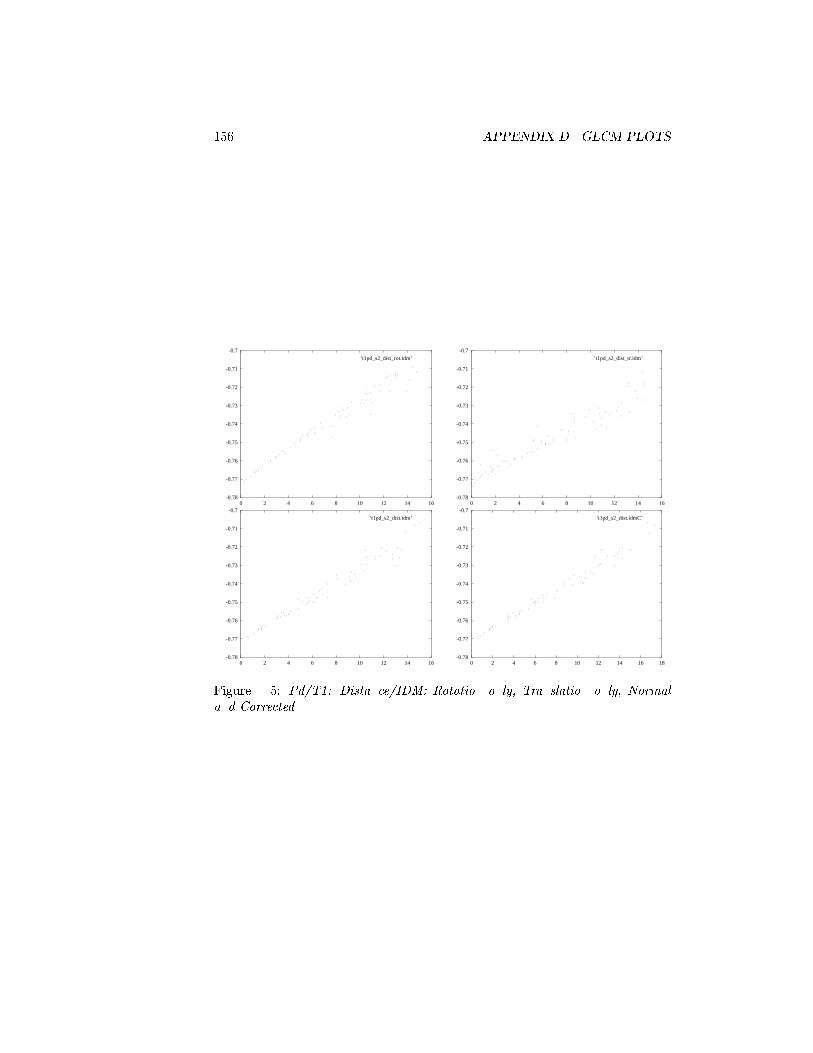
156 APPENDIX D. GLCM PLOTS
-0.78
-0.77
-0.76
-0.75
-0.74
-0.73
-0.72
-0.71
-0.7
0 2 4 6 8 10 12 14 16
’t1pd_s2_dist_rot.idm’
-0.78
-0.77
-0.76
-0.75
-0.74
-0.73
-0.72
-0.71
-0.7
0 2 4 6 8 10 12 14 16
’t1pd_s2_dist_tr.idm’
-0.78
-0.77
-0.76
-0.75
-0.74
-0.73
-0.72
-0.71
-0.7
0 2 4 6 8 10 12 14 16
’t1pd_s2_dist.idm’
-0.78
-0.77
-0.76
-0.75
-0.74
-0.73
-0.72
-0.71
-0.7
0 2 4 6 8 10 12 14 16 18
’t1pd_s2_dist.idmC’
Figure D.5: Pd/T1: Distance/IDM: Rotation only, Translation only, Normaland Corrected.
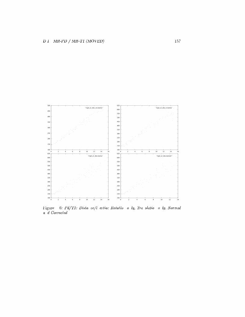
D.1. MR-PD / MR-T1 (MOVED) 157
100
150
200
250
300
350
400
450
500
0 2 4 6 8 10 12 14 16
’t1pd_s2_dist_rot.inertia’
100
150
200
250
300
350
400
450
500
550
600
650
0 2 4 6 8 10 12 14 16
’t1pd_s2_dist_tr.inertia’
100
150
200
250
300
350
400
450
500
550
600
650
0 2 4 6 8 10 12 14 16
’t1pd_s2_dist.inertia’
100
150
200
250
300
350
400
450
500
550
600
650
0 2 4 6 8 10 12 14
’t1pd_s2_dist.inertiaC’
Figure D.6: Pd/T1: Distance/inertia: Rotation only, Translation only, Normaland Corrected.

158 APPENDIX D. GLCM PLOTS
450
500
550
600
650
700
750
800
850
0 2 4 6 8 10 12 14 16
’t1pd_s2_dist_rot.dmoment’
450
500
550
600
650
700
750
800
850
900
0 2 4 6 8 10 12 14 16
’t1pd_s2_dist_tr.dmoment’
450
500
550
600
650
700
750
800
850
900
0 2 4 6 8 10 12 14 16
’t1pd_s2_dist.dmoment’
450
500
550
600
650
700
750
800
850
900
0 2 4 6 8 10 12 14 16
’t1pd_s2_dist.dmomentC’
Figure D.7: Pd/T1: Distance/Dmoment: Rotation only, Translation only, Nor-mal and Corrected.
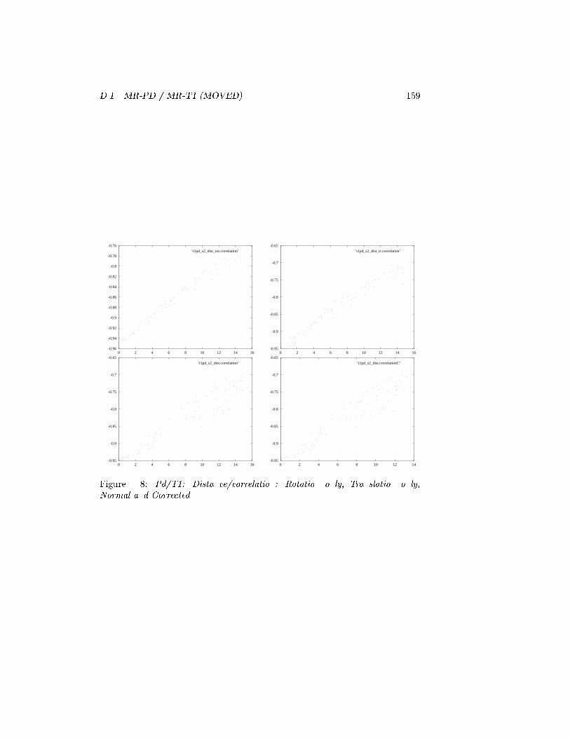
D.1. MR-PD / MR-T1 (MOVED) 159
-0.96
-0.94
-0.92
-0.9
-0.88
-0.86
-0.84
-0.82
-0.8
-0.78
-0.76
0 2 4 6 8 10 12 14 16
’t1pd_s2_dist_rot.correlation’
-0.95
-0.9
-0.85
-0.8
-0.75
-0.7
-0.65
0 2 4 6 8 10 12 14 16
’t1pd_s2_dist_tr.correlation’
-0.95
-0.9
-0.85
-0.8
-0.75
-0.7
-0.65
0 2 4 6 8 10 12 14 16
’t1pd_s2_dist.correlation’
-0.95
-0.9
-0.85
-0.8
-0.75
-0.7
-0.65
0 2 4 6 8 10 12 14
’t1pd_s2_dist.correlationC’
Figure D.8: Pd/T1: Distance/correlation: Rotation only, Translation only,Normal and Corrected.

160 APPENDIX D. GLCM PLOTS
-430000
-420000
-410000
-400000
-390000
-380000
-370000
-360000
-350000
-340000
0 2 4 6 8 10 12 14 16
’t1pd_s2_dist_rot.cshade’
-440000
-420000
-400000
-380000
-360000
-340000
-320000
0 2 4 6 8 10 12 14 16
’t1pd_s2_dist_tr.cshade’
-440000
-420000
-400000
-380000
-360000
-340000
-320000
0 2 4 6 8 10 12 14 16
’t1pd_s2_dist.cshade’
-440000
-420000
-400000
-380000
-360000
-340000
-320000
0 2 4 6 8 10 12 14
’t1pd_s2_dist.cshadeC’
Figure D.9: Pd/T1: Distance/Cshade: Rotation only, Translation only, Normaland Corrected.
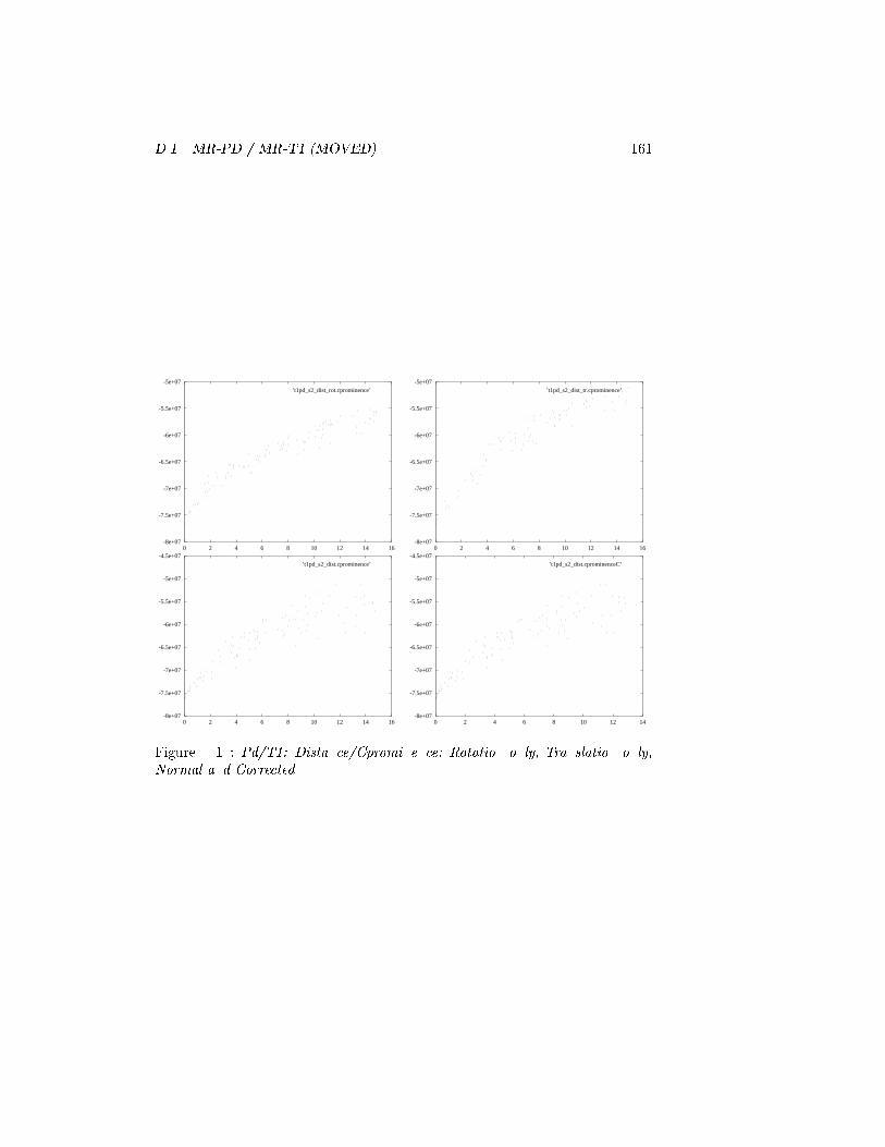
D.1. MR-PD / MR-T1 (MOVED) 161
-8e+07
-7.5e+07
-7e+07
-6.5e+07
-6e+07
-5.5e+07
-5e+07
0 2 4 6 8 10 12 14 16
’t1pd_s2_dist_rot.cprominence’
-8e+07
-7.5e+07
-7e+07
-6.5e+07
-6e+07
-5.5e+07
-5e+07
0 2 4 6 8 10 12 14 16
’t1pd_s2_dist_tr.cprominence’
-8e+07
-7.5e+07
-7e+07
-6.5e+07
-6e+07
-5.5e+07
-5e+07
-4.5e+07
0 2 4 6 8 10 12 14 16
’t1pd_s2_dist.cprominence’
-8e+07
-7.5e+07
-7e+07
-6.5e+07
-6e+07
-5.5e+07
-5e+07
-4.5e+07
0 2 4 6 8 10 12 14
’t1pd_s2_dist.cprominenceC’
Figure D.10: Pd/T1: Distance/Cprominence: Rotation only, Translation only,Normal and Corrected.

162 APPENDIX D. GLCM PLOTS
0
0.5
1
1.5
2
2.5
3
0 2 4 6 8 10 12 14 16
’t1pd_s2_dist_rot.woods_mrpet_xf’
0
0.5
1
1.5
2
2.5
3
3.5
0 2 4 6 8 10 12 14 16
’t1pd_s2_dist_tr.woods_mrpet_xf’
0
0.5
1
1.5
2
2.5
3
0 2 4 6 8 10 12 14 16
’t1pd_s2_dist.woods_mrpet_xf’
0
0.5
1
1.5
2
2.5
3
0 2 4 6 8 10 12 14 16 18
’t1pd_s2_dist.woods_mrpet_xfC’
Figure D.11: Pd/T1: Distance/Woods MR/PET X-xed: Rotation only, Trans-lation only, Normal and Corrected.
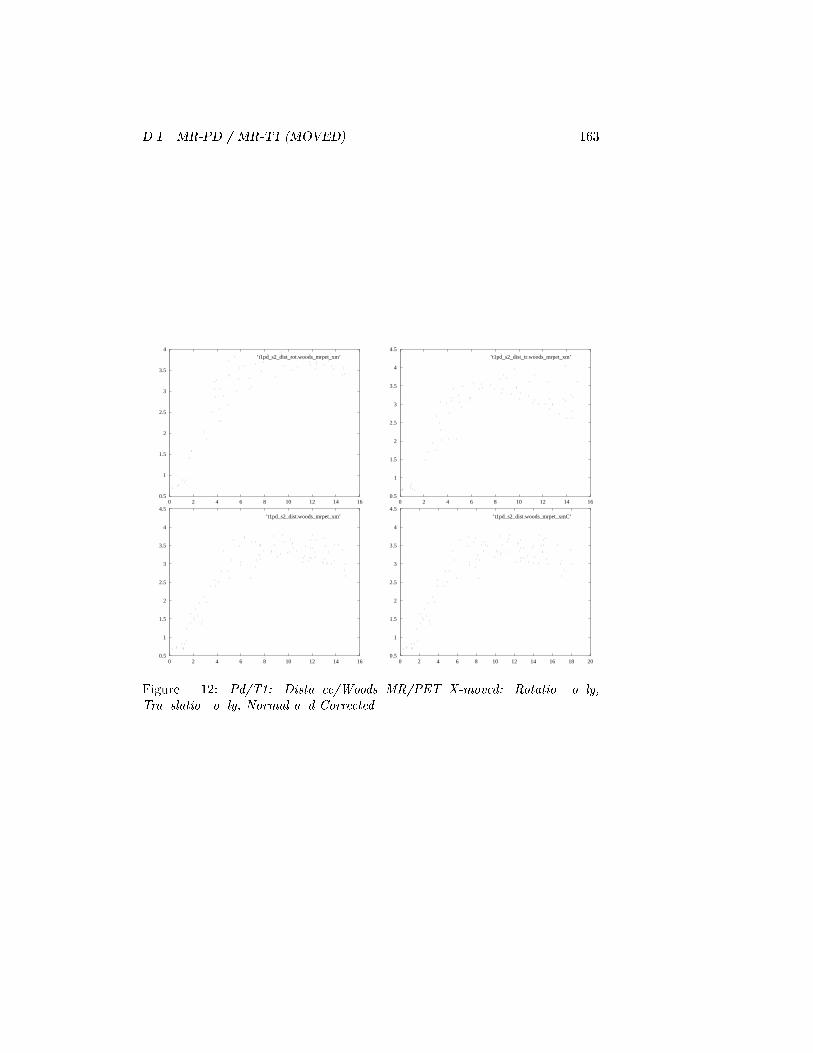
D.1. MR-PD / MR-T1 (MOVED) 163
0.5
1
1.5
2
2.5
3
3.5
4
0 2 4 6 8 10 12 14 16
’t1pd_s2_dist_rot.woods_mrpet_xm’
0.5
1
1.5
2
2.5
3
3.5
4
4.5
0 2 4 6 8 10 12 14 16
’t1pd_s2_dist_tr.woods_mrpet_xm’
0.5
1
1.5
2
2.5
3
3.5
4
4.5
0 2 4 6 8 10 12 14 16
’t1pd_s2_dist.woods_mrpet_xm’
0.5
1
1.5
2
2.5
3
3.5
4
4.5
0 2 4 6 8 10 12 14 16 18 20
’t1pd_s2_dist.woods_mrpet_xmC’
Figure D.12: Pd/T1: Distance/Woods MR/PET X-moved: Rotation only,Translation only, Normal and Corrected.

164 APPENDIX D. GLCM PLOTS
-0.31
-0.305
-0.3
-0.295
-0.29
-0.285
-0.28
-0.275
-0.27
-0.265
-0.26
-10 -8 -6 -4 -2 0 2 4 6 8 10
’t1pd_s2_seq21.tx.energy’’t1pd_s2_seq21.ty.energy’’t1pd_s2_seq21.tz.energy’’t1pd_s2_seq21.rx.energy’’t1pd_s2_seq21.ry.energy’’t1pd_s2_seq21.rz.energy’
Figure D.13: Pd/T1: Sequence plots of energy.
-0.31
-0.305
-0.3
-0.295
-0.29
-0.285
-0.28
-0.275
-0.27
-0.265
-0.26
-10 -8 -6 -4 -2 0 2 4 6 8 10
’t1pd_s2_seq21.tx.variance’’t1pd_s2_seq21.ty.variance’’t1pd_s2_seq21.tz.variance’’t1pd_s2_seq21.rx.variance’’t1pd_s2_seq21.ry.variance’’t1pd_s2_seq21.rz.variance’
Figure D.14: Pd/T1: Sequence plots of variance.

D.1. MR-PD / MR-T1 (MOVED) 165
2.8
2.85
2.9
2.95
3
3.05
3.1
3.15
3.2
3.25
-10 -8 -6 -4 -2 0 2 4 6 8 10
’t1pd_s2_seq21.tx.entropy’’t1pd_s2_seq21.ty.entropy’’t1pd_s2_seq21.tz.entropy’’t1pd_s2_seq21.rx.entropy’’t1pd_s2_seq21.ry.entropy’’t1pd_s2_seq21.rz.entropy’
Figure D.15: Pd/T1: Sequence plots of entropy.
-0.8
-0.75
-0.7
-0.65
-0.6
-0.55
-0.5
-10 -8 -6 -4 -2 0 2 4 6 8 10
’t1pd_s2_seq21.tx.mi’’t1pd_s2_seq21.ty.mi’’t1pd_s2_seq21.tz.mi’’t1pd_s2_seq21.rx.mi’’t1pd_s2_seq21.ry.mi’’t1pd_s2_seq21.rz.mi’
Figure D.16: Pd/T1: Sequence plots of MI.
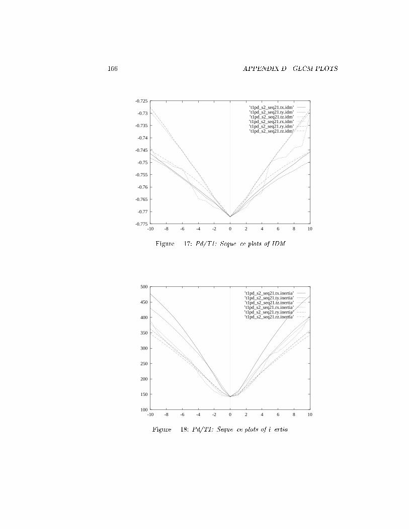
166 APPENDIX D. GLCM PLOTS
-0.775
-0.77
-0.765
-0.76
-0.755
-0.75
-0.745
-0.74
-0.735
-0.73
-0.725
-10 -8 -6 -4 -2 0 2 4 6 8 10
’t1pd_s2_seq21.tx.idm’’t1pd_s2_seq21.ty.idm’’t1pd_s2_seq21.tz.idm’’t1pd_s2_seq21.rx.idm’’t1pd_s2_seq21.ry.idm’’t1pd_s2_seq21.rz.idm’
Figure D.17: Pd/T1: Sequence plots of IDM.
100
150
200
250
300
350
400
450
500
-10 -8 -6 -4 -2 0 2 4 6 8 10
’t1pd_s2_seq21.tx.inertia’’t1pd_s2_seq21.ty.inertia’’t1pd_s2_seq21.tz.inertia’’t1pd_s2_seq21.rx.inertia’’t1pd_s2_seq21.ry.inertia’’t1pd_s2_seq21.rz.inertia’
Figure D.18: Pd/T1: Sequence plots of inertia.
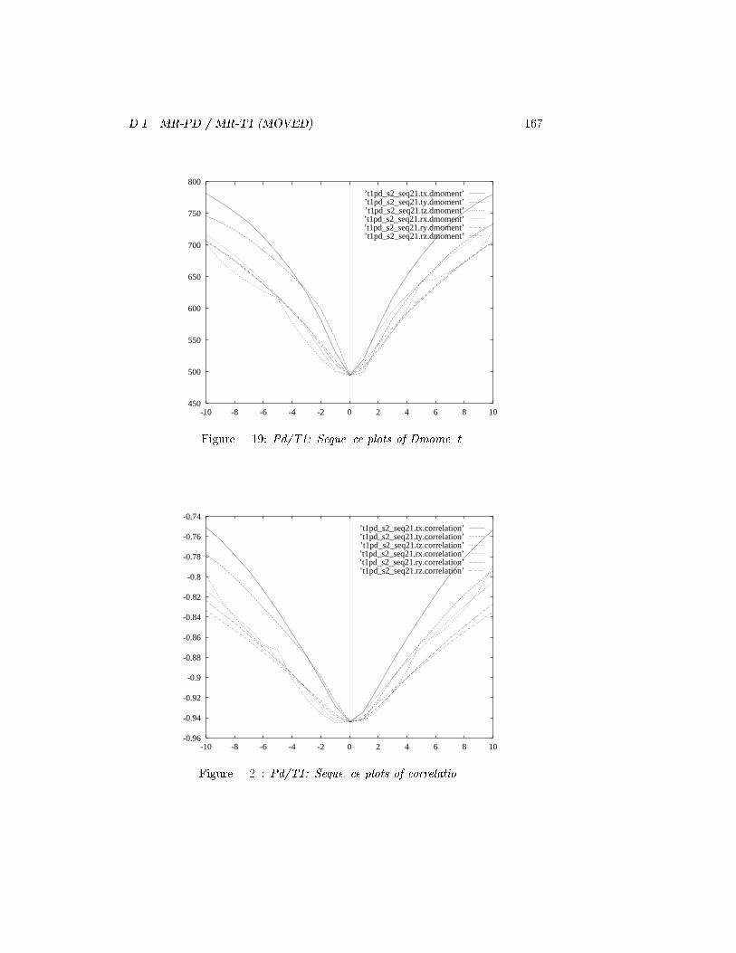
D.1. MR-PD / MR-T1 (MOVED) 167
450
500
550
600
650
700
750
800
-10 -8 -6 -4 -2 0 2 4 6 8 10
’t1pd_s2_seq21.tx.dmoment’’t1pd_s2_seq21.ty.dmoment’’t1pd_s2_seq21.tz.dmoment’’t1pd_s2_seq21.rx.dmoment’’t1pd_s2_seq21.ry.dmoment’’t1pd_s2_seq21.rz.dmoment’
Figure D.19: Pd/T1: Sequence plots of Dmoment.
-0.96
-0.94
-0.92
-0.9
-0.88
-0.86
-0.84
-0.82
-0.8
-0.78
-0.76
-0.74
-10 -8 -6 -4 -2 0 2 4 6 8 10
’t1pd_s2_seq21.tx.correlation’’t1pd_s2_seq21.ty.correlation’’t1pd_s2_seq21.tz.correlation’’t1pd_s2_seq21.rx.correlation’’t1pd_s2_seq21.ry.correlation’’t1pd_s2_seq21.rz.correlation’
Figure D.20: Pd/T1: Sequence plots of correlation.
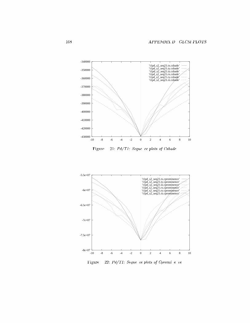
168 APPENDIX D. GLCM PLOTS
-430000
-420000
-410000
-400000
-390000
-380000
-370000
-360000
-350000
-340000
-10 -8 -6 -4 -2 0 2 4 6 8 10
’t1pd_s2_seq21.tx.cshade’’t1pd_s2_seq21.ty.cshade’’t1pd_s2_seq21.tz.cshade’’t1pd_s2_seq21.rx.cshade’’t1pd_s2_seq21.ry.cshade’’t1pd_s2_seq21.rz.cshade’
Figure D.21: Pd/T1: Sequence plots of Cshade.
-8e+07
-7.5e+07
-7e+07
-6.5e+07
-6e+07
-5.5e+07
-10 -8 -6 -4 -2 0 2 4 6 8 10
’t1pd_s2_seq21.tx.cprominence’’t1pd_s2_seq21.ty.cprominence’’t1pd_s2_seq21.tz.cprominence’’t1pd_s2_seq21.rx.cprominence’’t1pd_s2_seq21.ry.cprominence’’t1pd_s2_seq21.rz.cprominence’
Figure D.22: Pd/T1: Sequence plots of Cprominence.

D.1. MR-PD / MR-T1 (MOVED) 169
0
0.5
1
1.5
2
2.5
3
-10 -8 -6 -4 -2 0 2 4 6 8 10
’t1pd_s2_seq21.tx.woods_mrpet_xf’’t1pd_s2_seq21.ty.woods_mrpet_xf’’t1pd_s2_seq21.tz.woods_mrpet_xf’’t1pd_s2_seq21.rx.woods_mrpet_xf’’t1pd_s2_seq21.ry.woods_mrpet_xf’’t1pd_s2_seq21.rz.woods_mrpet_xf’
Figure D.23: Pd/T1: Sequence plots of woods MR/PET X-xed.
0.5
1
1.5
2
2.5
3
3.5
4
4.5
-10 -8 -6 -4 -2 0 2 4 6 8 10
’t1pd_s2_seq21.tx.woods_mrpet_xm’’t1pd_s2_seq21.ty.woods_mrpet_xm’’t1pd_s2_seq21.tz.woods_mrpet_xm’’t1pd_s2_seq21.rx.woods_mrpet_xm’’t1pd_s2_seq21.ry.woods_mrpet_xm’’t1pd_s2_seq21.rz.woods_mrpet_xm’
Figure D.24: Pd/T1: Sequence plots of woods MR/PET X-moved.

170 APPENDIX D. GLCM PLOTS
D.2 CT Bone / MR-T1 (moved)
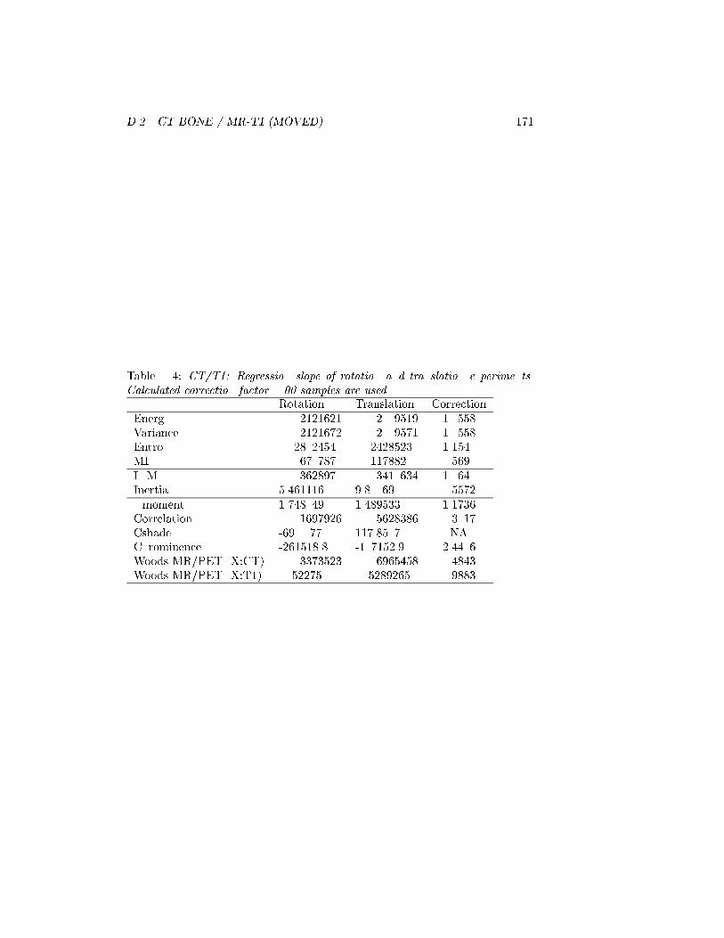
D.2. CT BONE / MR-T1 (MOVED) 171
Table D.4: CT/T1: Regression slope of rotation and translation experiments.Calculated correction factor. 500 samples are used.
Rotation Translation CorrectionEnergy 0.002121621 0.002009519 1.0558Variance 0.002121672 0.002009571 1.0558Entropy 0.02802454 0.02428523 1.1540MI 0.00670787 0.0117882 0.5690IDM 0.00362897 0.003410634 1.0640Inertia 5.461116 9.80069 0.5572Dmoment 1.748049 1.489533 1.1736Correlation 0.001697926 0.005628386 0.3017Cshade -690.077 117.8507 NACprominence -261518.8 -107152.9 2.4406Woods MR/PET (X:CT) 0.003373523 0.006965458 0.4843Woods MR/PET (X:T1) -0.52275 -0.5289265 0.9883
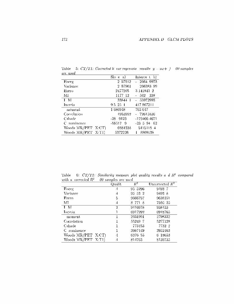
172 APPENDIX D. GLCM PLOTS
Table D.5: CT/T1: Corrected linear regression results (y = ax+b). 500 samplesare used.
Slope (a) Intercept (b)Energy 0.002057912 -0.266409973Variance 0.002057961 -0.266383099Entropy 0.02477265 3.14184302MI 0.01177012 -0.56200238IDM 0.003384401 -0.559729930Inertia 9.502501 417.867211Dmoment 1.686948 763.647000Correlation 0.004953982 -0.726158360Cshade -280.9123 -179466.4671Cprominence -88517.09 -23050940.62Woods MR/PET (X:CT) 0.006881338 0.511511804Woods MR/PET (X:T1) -0.5372226 10.8869138
Table D.6: CT/T1: Similarity measure plot quality results and R2 comparedwith uncorrected R2. 500 samples are used.
Quality R2 Uncorrected R2
Energy 4 0.9505296 0.9493070Variance 4 0.9505302 0.9493080Entropy 5 0.9666757 0.9638251MI 4 0.8077108 0.7595025IDM 2 0.9416978 0.9384330Inertia 1 0.6917992 0.6948765Dmoment 1 0.2931991 0.2798332Correlation 1 0.5524907 0.5277128Cshade 1 0.0773453 0.0773202Cprominence 1 0.3667449 0.3952463Woods MR/PET (X:CT) 4 0.6376055 0.6018653Woods MR/PET (X:T1) 4 0.8147630 0.8139735

D.2. CT BONE / MR-T1 (MOVED) 173
-0.27
-0.265
-0.26
-0.255
-0.25
-0.245
-0.24
-0.235
-0.23
0 2 4 6 8 10 12 14 16
’t1ct_s2_dist_rot.energy’
-0.3
-0.29
-0.28
-0.27
-0.26
-0.25
-0.24
-0.23
0 2 4 6 8 10 12 14 16
’t1ct_s2_dist_tr.energy’
-0.27
-0.265
-0.26
-0.255
-0.25
-0.245
-0.24
-0.235
-0.23
-0.225
0 2 4 6 8 10 12 14 16
’t1ct_s2_dist.energy’
-0.27
-0.265
-0.26
-0.255
-0.25
-0.245
-0.24
-0.235
-0.23
-0.225
0 5 10 15 20 25
’t1ct_s2_dist.energyC’
Figure D.25: CT/T1: Distance/energy: Rotation only, Translation only, Nor-mal and Corrected.
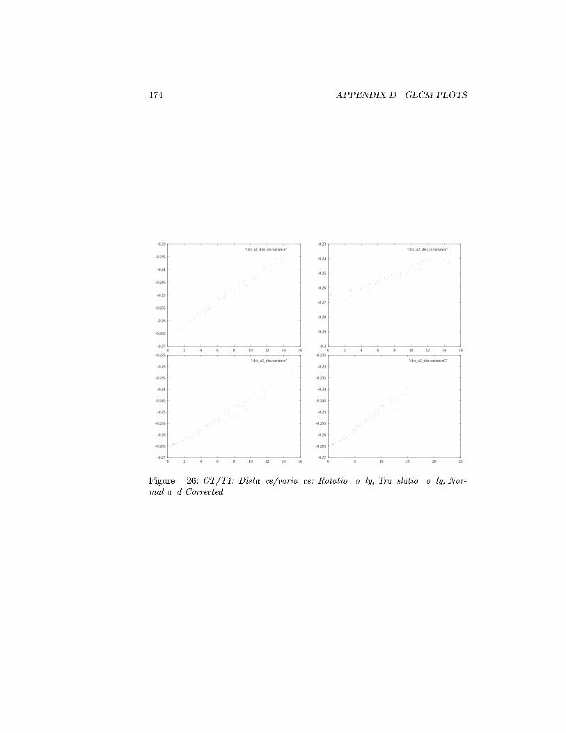
174 APPENDIX D. GLCM PLOTS
-0.27
-0.265
-0.26
-0.255
-0.25
-0.245
-0.24
-0.235
-0.23
0 2 4 6 8 10 12 14 16
’t1ct_s2_dist_rot.variance’
-0.3
-0.29
-0.28
-0.27
-0.26
-0.25
-0.24
-0.23
0 2 4 6 8 10 12 14 16
’t1ct_s2_dist_tr.variance’
-0.27
-0.265
-0.26
-0.255
-0.25
-0.245
-0.24
-0.235
-0.23
-0.225
0 2 4 6 8 10 12 14 16
’t1ct_s2_dist.variance’
-0.27
-0.265
-0.26
-0.255
-0.25
-0.245
-0.24
-0.235
-0.23
-0.225
0 5 10 15 20 25
’t1ct_s2_dist.varianceC’
Figure D.26: CT/T1: Distance/variance: Rotation only, Translation only, Nor-mal and Corrected.

D.2. CT BONE / MR-T1 (MOVED) 175
3.1
3.15
3.2
3.25
3.3
3.35
3.4
3.45
3.5
3.55
3.6
0 2 4 6 8 10 12 14 16
’t1ct_s2_dist_rot.entropy’
3.1
3.15
3.2
3.25
3.3
3.35
3.4
3.45
3.5
3.55
0 2 4 6 8 10 12 14 16
’t1ct_s2_dist_tr.entropy’
3.1
3.15
3.2
3.25
3.3
3.35
3.4
3.45
3.5
3.55
3.6
0 2 4 6 8 10 12 14 16
’t1ct_s2_dist.entropy’
3.1
3.15
3.2
3.25
3.3
3.35
3.4
3.45
3.5
3.55
3.6
0 2 4 6 8 10 12 14 16 18
’t1ct_s2_dist.entropyC’
Figure D.27: CT/T1: Distance/entropy: Rotation only, Translation only, Nor-mal and Corrected.
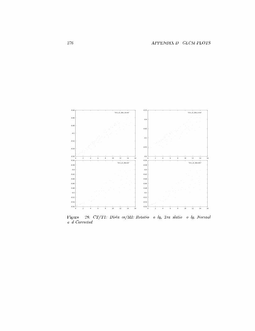
176 APPENDIX D. GLCM PLOTS
-0.56
-0.54
-0.52
-0.5
-0.48
-0.46
-0.44
0 2 4 6 8 10 12 14 16
’t1ct_s2_dist_rot.mi’
-0.6
-0.55
-0.5
-0.45
-0.4
-0.35
0 2 4 6 8 10 12 14 16
’t1ct_s2_dist_tr.mi’
-0.56
-0.54
-0.52
-0.5
-0.48
-0.46
-0.44
-0.42
-0.4
-0.38
-0.36
0 2 4 6 8 10 12 14 16
’t1ct_s2_dist.mi’
-0.56
-0.54
-0.52
-0.5
-0.48
-0.46
-0.44
-0.42
-0.4
-0.38
-0.36
0 2 4 6 8 10 12 14 16
’t1ct_s2_dist.miC’
Figure D.28: CT/T1: Distance/MI: Rotation only, Translation only, Normaland Corrected.
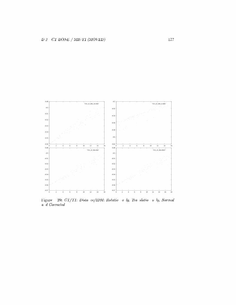
D.2. CT BONE / MR-T1 (MOVED) 177
-0.56
-0.55
-0.54
-0.53
-0.52
-0.51
-0.5
-0.49
0 2 4 6 8 10 12 14 16
’t1ct_s2_dist_rot.idm’
-0.62
-0.6
-0.58
-0.56
-0.54
-0.52
-0.5
0 2 4 6 8 10 12 14 16
’t1ct_s2_dist_tr.idm’
-0.57
-0.56
-0.55
-0.54
-0.53
-0.52
-0.51
-0.5
-0.49
0 2 4 6 8 10 12 14 16
’t1ct_s2_dist.idm’
-0.57
-0.56
-0.55
-0.54
-0.53
-0.52
-0.51
-0.5
-0.49
0 2 4 6 8 10 12 14 16 18
’t1ct_s2_dist.idmC’
Figure D.29: CT/T1: Distance/IDM: Rotation only, Translation only, Normaland Corrected.

178 APPENDIX D. GLCM PLOTS
420
440
460
480
500
520
540
560
0 2 4 6 8 10 12 14 16
’t1ct_s2_dist_rot.inertia’
400
420
440
460
480
500
520
540
560
580
600
620
0 2 4 6 8 10 12 14 16
’t1ct_s2_dist_tr.inertia’
400
420
440
460
480
500
520
540
560
580
600
620
0 2 4 6 8 10 12 14 16
’t1ct_s2_dist.inertia’
400
420
440
460
480
500
520
540
560
580
600
620
0 2 4 6 8 10 12 14
’t1ct_s2_dist.inertiaC’
Figure D.30: CT/T1: Distance/inertia: Rotation only, Translation only, Nor-mal and Corrected.

D.2. CT BONE / MR-T1 (MOVED) 179
760
770
780
790
800
810
820
830
0 2 4 6 8 10 12 14 16
’t1ct_s2_dist_rot.dmoment’
730
740
750
760
770
780
790
800
810
820
0 2 4 6 8 10 12 14 16
’t1ct_s2_dist_tr.dmoment’
740
750
760
770
780
790
800
810
820
830
840
0 2 4 6 8 10 12 14 16
’t1ct_s2_dist.dmoment’
740
750
760
770
780
790
800
810
820
830
840
0 2 4 6 8 10 12 14 16
’t1ct_s2_dist.dmomentC’
Figure D.31: CT/T1: Distance/Dmoment: Rotation only, Translation only,Normal and Corrected.
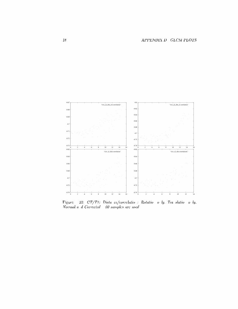
180 APPENDIX D. GLCM PLOTS
-0.73
-0.72
-0.71
-0.7
-0.69
-0.68
-0.67
0 2 4 6 8 10 12 14 16
’t1ct_s2_dist_rot.correlation’
-0.74
-0.72
-0.7
-0.68
-0.66
-0.64
-0.62
-0.6
0 2 4 6 8 10 12 14 16
’t1ct_s2_dist_tr.correlation’
-0.74
-0.72
-0.7
-0.68
-0.66
-0.64
-0.62
0 2 4 6 8 10 12 14 16
’t1ct_s2_dist.correlation’
-0.74
-0.72
-0.7
-0.68
-0.66
-0.64
-0.62
0 2 4 6 8 10 12 14
’t1ct_s2_dist.correlationC’
Figure D.32: CT/T1: Distance/correlation: Rotation only, Translation only,Normal and Corrected. 500 samples are used.
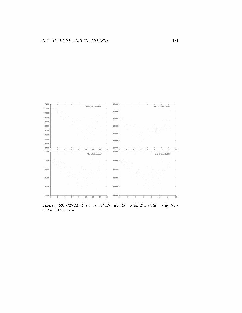
D.2. CT BONE / MR-T1 (MOVED) 181
-194000
-192000
-190000
-188000
-186000
-184000
-182000
-180000
-178000
-176000
-174000
0 2 4 6 8 10 12 14 16
’t1ct_s2_dist_rot.cshade’
-195000
-190000
-185000
-180000
-175000
-170000
-165000
0 2 4 6 8 10 12 14 16
’t1ct_s2_dist_tr.cshade’
-195000
-190000
-185000
-180000
-175000
-170000
0 2 4 6 8 10 12 14 16
’t1ct_s2_dist.cshade’
-195000
-190000
-185000
-180000
-175000
-170000
0 2 4 6 8 10 12 14
’t1ct_s2_dist.cshadeC’
Figure D.33: CT/T1: Distance/Cshade: Rotation only, Translation only, Nor-mal and Corrected.

182 APPENDIX D. GLCM PLOTS
-2.8e+07
-2.7e+07
-2.6e+07
-2.5e+07
-2.4e+07
-2.3e+07
-2.2e+07
0 2 4 6 8 10 12 14 16
’t1ct_s2_dist_rot.cprominence’
-2.7e+07
-2.6e+07
-2.5e+07
-2.4e+07
-2.3e+07
-2.2e+07
-2.1e+07
0 2 4 6 8 10 12 14 16
’t1ct_s2_dist_tr.cprominence’
-2.8e+07
-2.7e+07
-2.6e+07
-2.5e+07
-2.4e+07
-2.3e+07
-2.2e+07
-2.1e+07
0 2 4 6 8 10 12 14 16
’t1ct_s2_dist.cprominence’
-2.8e+07
-2.7e+07
-2.6e+07
-2.5e+07
-2.4e+07
-2.3e+07
-2.2e+07
-2.1e+07
0 2 4 6 8 10 12 14
’t1ct_s2_dist.cprominenceC’
Figure D.34: CT/T1: Distance/Cprominence: Rotation only, Translation only,Normal and Corrected. 500 samples are used.

D.2. CT BONE / MR-T1 (MOVED) 183
0.5
0.51
0.52
0.53
0.54
0.55
0.56
0.57
0.58
0 2 4 6 8 10 12 14 16
’t1ct_s2_dist_rot.woods_mrpet_xf’
0.48
0.5
0.52
0.54
0.56
0.58
0.6
0.62
0.64
0.66
0 2 4 6 8 10 12 14 16
’t1ct_s2_dist_tr.woods_mrpet_xf’
0.5
0.52
0.54
0.56
0.58
0.6
0.62
0.64
0 2 4 6 8 10 12 14 16
’t1ct_s2_dist.woods_mrpet_xf’
0.5
0.52
0.54
0.56
0.58
0.6
0.62
0.64
0 2 4 6 8 10 12 14 16 18
’t1ct_s2_dist.woods_mrpet_xfC’
Figure D.35: CT/T1: Distance/Woods MR/PET X-xed: Rotation only, Trans-lation only, Normal and Corrected.
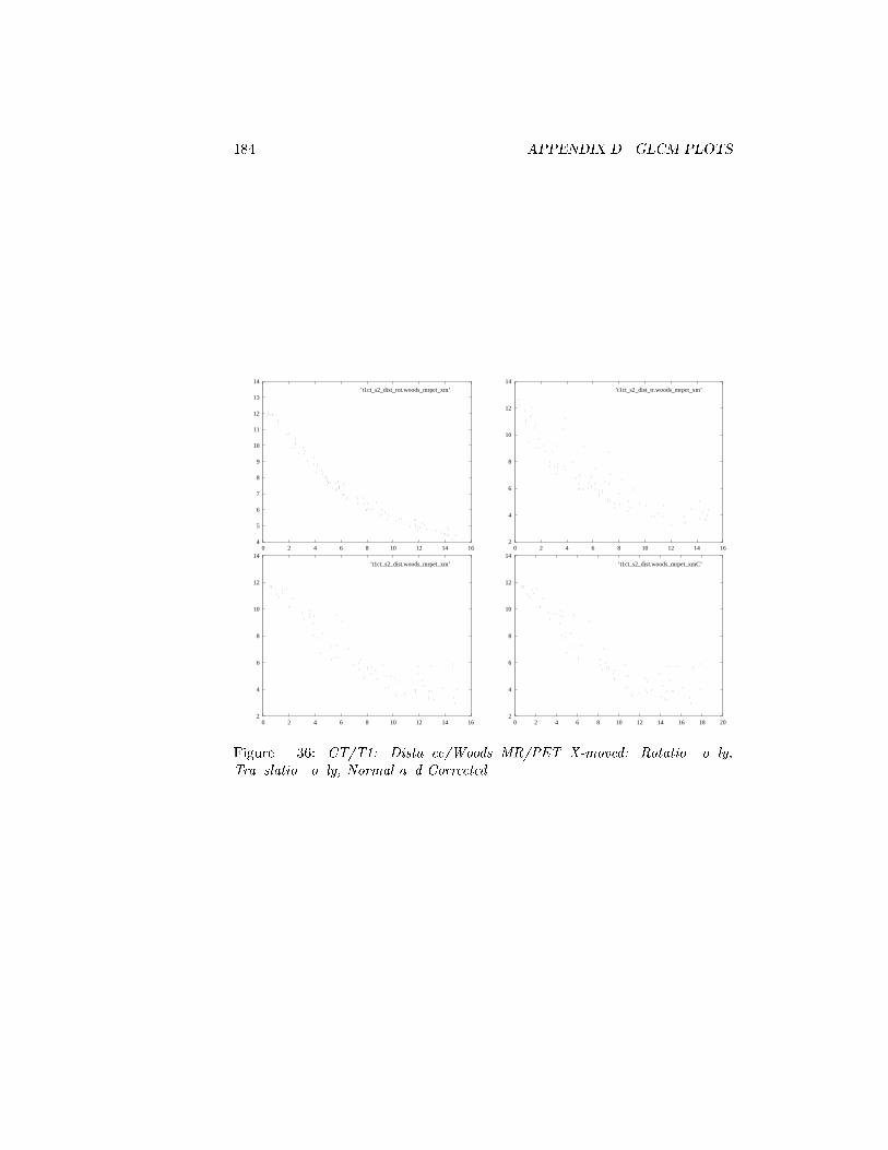
184 APPENDIX D. GLCM PLOTS
4
5
6
7
8
9
10
11
12
13
14
0 2 4 6 8 10 12 14 16
’t1ct_s2_dist_rot.woods_mrpet_xm’
2
4
6
8
10
12
14
0 2 4 6 8 10 12 14 16
’t1ct_s2_dist_tr.woods_mrpet_xm’
2
4
6
8
10
12
14
0 2 4 6 8 10 12 14 16
’t1ct_s2_dist.woods_mrpet_xm’
2
4
6
8
10
12
14
0 2 4 6 8 10 12 14 16 18 20
’t1ct_s2_dist.woods_mrpet_xmC’
Figure D.36: CT/T1: Distance/Woods MR/PET X-moved: Rotation only,Translation only, Normal and Corrected.
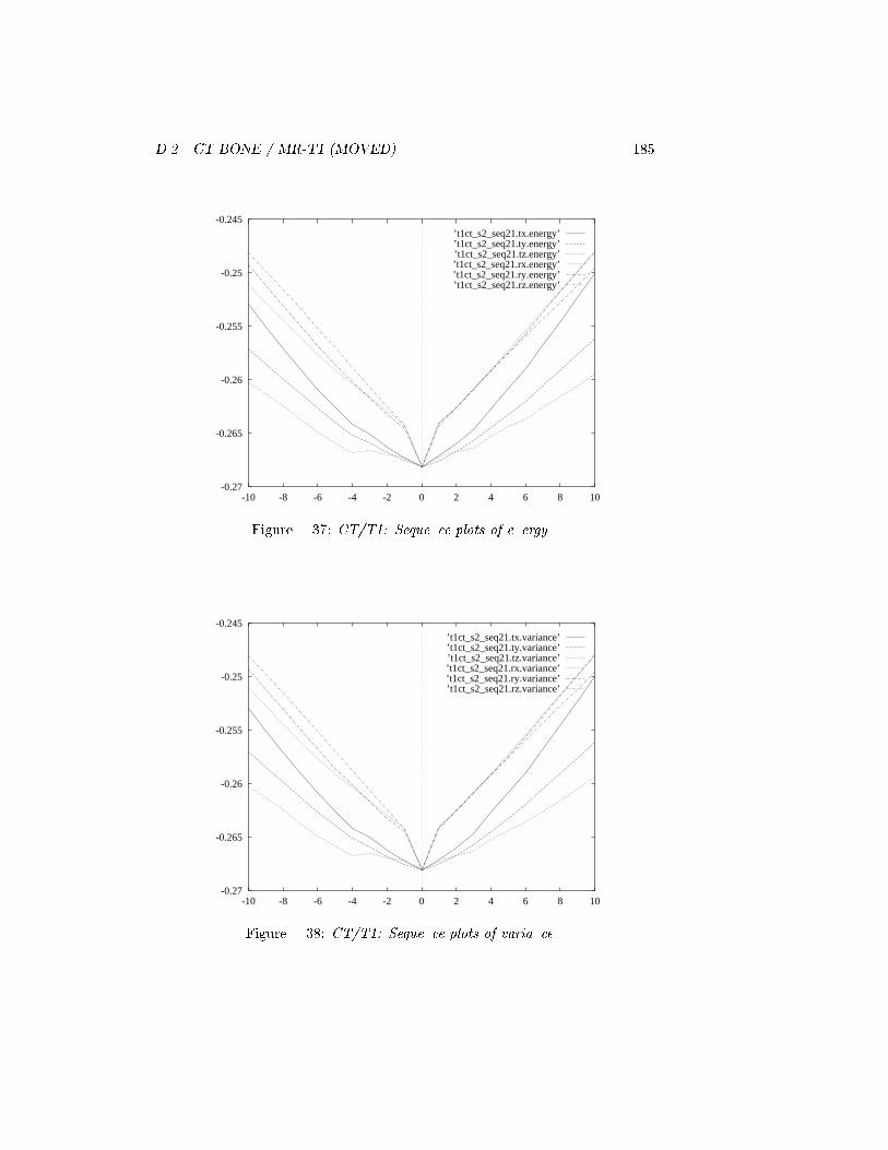
D.2. CT BONE / MR-T1 (MOVED) 185
-0.27
-0.265
-0.26
-0.255
-0.25
-0.245
-10 -8 -6 -4 -2 0 2 4 6 8 10
’t1ct_s2_seq21.tx.energy’’t1ct_s2_seq21.ty.energy’’t1ct_s2_seq21.tz.energy’’t1ct_s2_seq21.rx.energy’’t1ct_s2_seq21.ry.energy’’t1ct_s2_seq21.rz.energy’
Figure D.37: CT/T1: Sequence plots of energy.
-0.27
-0.265
-0.26
-0.255
-0.25
-0.245
-10 -8 -6 -4 -2 0 2 4 6 8 10
’t1ct_s2_seq21.tx.variance’’t1ct_s2_seq21.ty.variance’’t1ct_s2_seq21.tz.variance’’t1ct_s2_seq21.rx.variance’’t1ct_s2_seq21.ry.variance’’t1ct_s2_seq21.rz.variance’
Figure D.38: CT/T1: Sequence plots of variance.
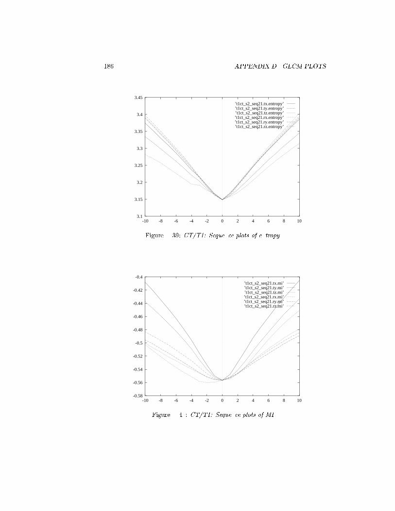
186 APPENDIX D. GLCM PLOTS
3.1
3.15
3.2
3.25
3.3
3.35
3.4
3.45
-10 -8 -6 -4 -2 0 2 4 6 8 10
’t1ct_s2_seq21.tx.entropy’’t1ct_s2_seq21.ty.entropy’’t1ct_s2_seq21.tz.entropy’’t1ct_s2_seq21.rx.entropy’’t1ct_s2_seq21.ry.entropy’’t1ct_s2_seq21.rz.entropy’
Figure D.39: CT/T1: Sequence plots of entropy.
-0.58
-0.56
-0.54
-0.52
-0.5
-0.48
-0.46
-0.44
-0.42
-0.4
-10 -8 -6 -4 -2 0 2 4 6 8 10
’t1ct_s2_seq21.tx.mi’’t1ct_s2_seq21.ty.mi’’t1ct_s2_seq21.tz.mi’’t1ct_s2_seq21.rx.mi’’t1ct_s2_seq21.ry.mi’’t1ct_s2_seq21.rz.mi’
Figure D.40: CT/T1: Sequence plots of MI.
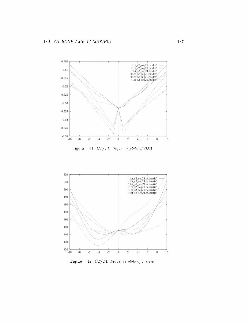
D.2. CT BONE / MR-T1 (MOVED) 187
-0.55
-0.545
-0.54
-0.535
-0.53
-0.525
-0.52
-0.515
-0.51
-0.505
-10 -8 -6 -4 -2 0 2 4 6 8 10
’t1ct_s2_seq21.tx.idm’’t1ct_s2_seq21.ty.idm’’t1ct_s2_seq21.tz.idm’’t1ct_s2_seq21.rx.idm’’t1ct_s2_seq21.ry.idm’’t1ct_s2_seq21.rz.idm’
Figure D.41: CT/T1: Sequence plots of IDM.
420
430
440
450
460
470
480
490
500
510
520
-10 -8 -6 -4 -2 0 2 4 6 8 10
’t1ct_s2_seq21.tx.inertia’’t1ct_s2_seq21.ty.inertia’’t1ct_s2_seq21.tz.inertia’’t1ct_s2_seq21.rx.inertia’’t1ct_s2_seq21.ry.inertia’’t1ct_s2_seq21.rz.inertia’
Figure D.42: CT/T1: Sequence plots of inertia.

188 APPENDIX D. GLCM PLOTS
740
750
760
770
780
790
800
810
-10 -8 -6 -4 -2 0 2 4 6 8 10
’t1ct_s2_seq21.tx.dmoment’’t1ct_s2_seq21.ty.dmoment’’t1ct_s2_seq21.tz.dmoment’’t1ct_s2_seq21.rx.dmoment’’t1ct_s2_seq21.ry.dmoment’’t1ct_s2_seq21.rz.dmoment’
Figure D.43: CT/T1: Sequence plots of Dmoment.
-0.73
-0.72
-0.71
-0.7
-0.69
-0.68
-0.67
-10 -8 -6 -4 -2 0 2 4 6 8 10
’t1ct_s2_seq21.tx.correlation’’t1ct_s2_seq21.ty.correlation’’t1ct_s2_seq21.tz.correlation’’t1ct_s2_seq21.rx.correlation’’t1ct_s2_seq21.ry.correlation’’t1ct_s2_seq21.rz.correlation’
Figure D.44: CT/T1: Sequence plots of correlation.
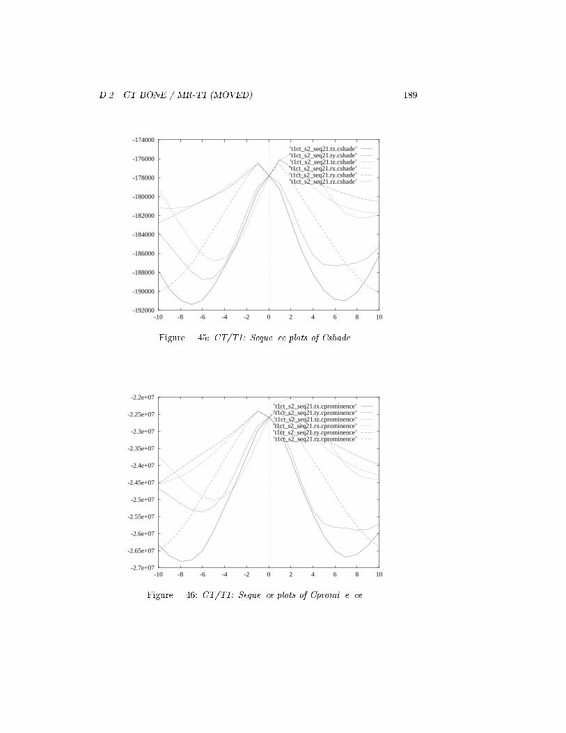
D.2. CT BONE / MR-T1 (MOVED) 189
-192000
-190000
-188000
-186000
-184000
-182000
-180000
-178000
-176000
-174000
-10 -8 -6 -4 -2 0 2 4 6 8 10
’t1ct_s2_seq21.tx.cshade’’t1ct_s2_seq21.ty.cshade’’t1ct_s2_seq21.tz.cshade’’t1ct_s2_seq21.rx.cshade’’t1ct_s2_seq21.ry.cshade’’t1ct_s2_seq21.rz.cshade’
Figure D.45: CT/T1: Sequence plots of Cshade.
-2.7e+07
-2.65e+07
-2.6e+07
-2.55e+07
-2.5e+07
-2.45e+07
-2.4e+07
-2.35e+07
-2.3e+07
-2.25e+07
-2.2e+07
-10 -8 -6 -4 -2 0 2 4 6 8 10
’t1ct_s2_seq21.tx.cprominence’’t1ct_s2_seq21.ty.cprominence’’t1ct_s2_seq21.tz.cprominence’’t1ct_s2_seq21.rx.cprominence’’t1ct_s2_seq21.ry.cprominence’’t1ct_s2_seq21.rz.cprominence’
Figure D.46: CT/T1: Sequence plots of Cprominence.
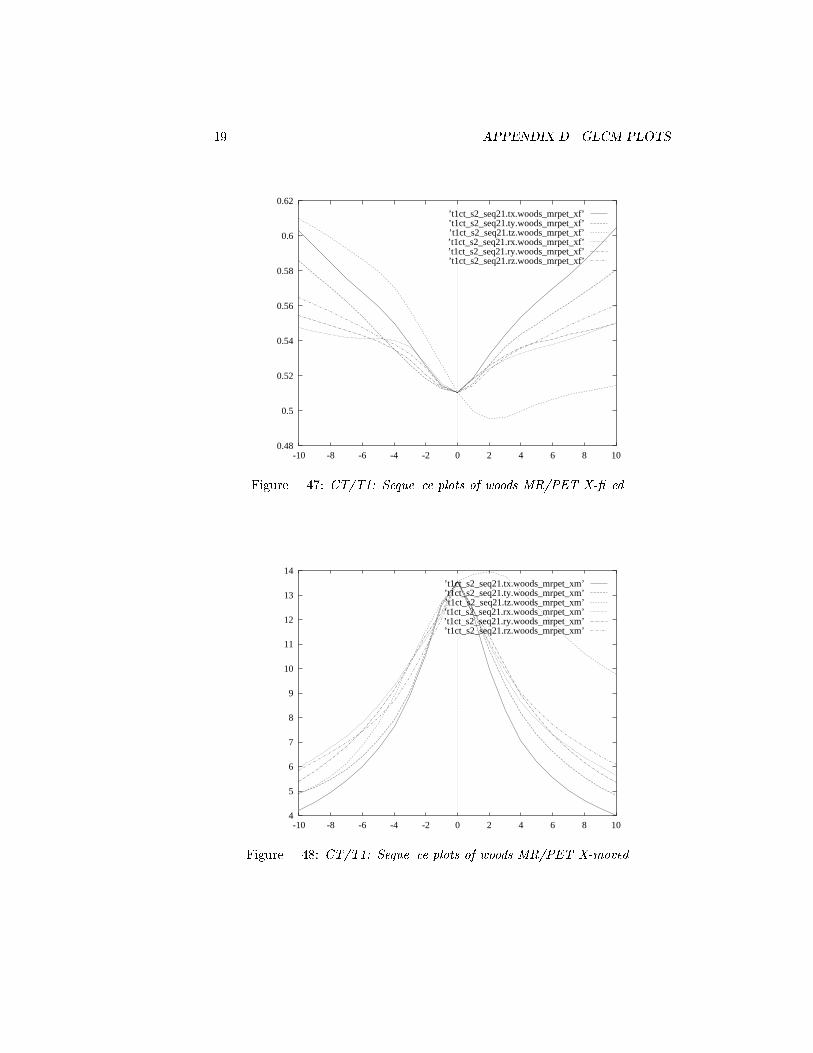
190 APPENDIX D. GLCM PLOTS
0.48
0.5
0.52
0.54
0.56
0.58
0.6
0.62
-10 -8 -6 -4 -2 0 2 4 6 8 10
’t1ct_s2_seq21.tx.woods_mrpet_xf’’t1ct_s2_seq21.ty.woods_mrpet_xf’’t1ct_s2_seq21.tz.woods_mrpet_xf’’t1ct_s2_seq21.rx.woods_mrpet_xf’’t1ct_s2_seq21.ry.woods_mrpet_xf’’t1ct_s2_seq21.rz.woods_mrpet_xf’
Figure D.47: CT/T1: Sequence plots of woods MR/PET X-xed.
4
5
6
7
8
9
10
11
12
13
14
-10 -8 -6 -4 -2 0 2 4 6 8 10
’t1ct_s2_seq21.tx.woods_mrpet_xm’’t1ct_s2_seq21.ty.woods_mrpet_xm’’t1ct_s2_seq21.tz.woods_mrpet_xm’’t1ct_s2_seq21.rx.woods_mrpet_xm’’t1ct_s2_seq21.ry.woods_mrpet_xm’’t1ct_s2_seq21.rz.woods_mrpet_xm’
Figure D.48: CT/T1: Sequence plots of woods MR/PET X-moved.

D.3. CT BONE (MOVED) / RED 191
D.3 CT Bone (moved) / Red
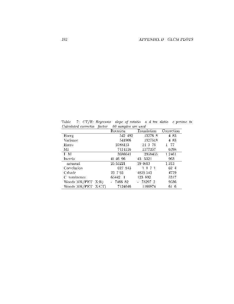
192 APPENDIX D. GLCM PLOTS
Table D.7: CT/R: Regression slope of rotation and translation experiments.Calculated correction factor. 500 samples are used.
Rotation Translation CorrectionEnergy 0.0005420492 0.001327608 0.4083Variance 0.000541966 0.001327518 0.4083Entropy 0.02588123 0.02403076 1.0770MI 0.007414116 0.01177257 0.6298IDM 0.003686641 0.002958455 1.2461Inertia 41.46096 43.05321 0.9630Dmoment 25.55221 19.4613 1.3130Correlation 0.006270843 0.01010701 0.6204Cshade 2307.93 4829.543 0.4779Cprominence 654420.1 1230892 0.5317Woods MR/PET (X:R) -0.7466082 -0.7829702 0.9536Woods MR/PET (X:CT) 0.007124646 0.01166874 0.6106
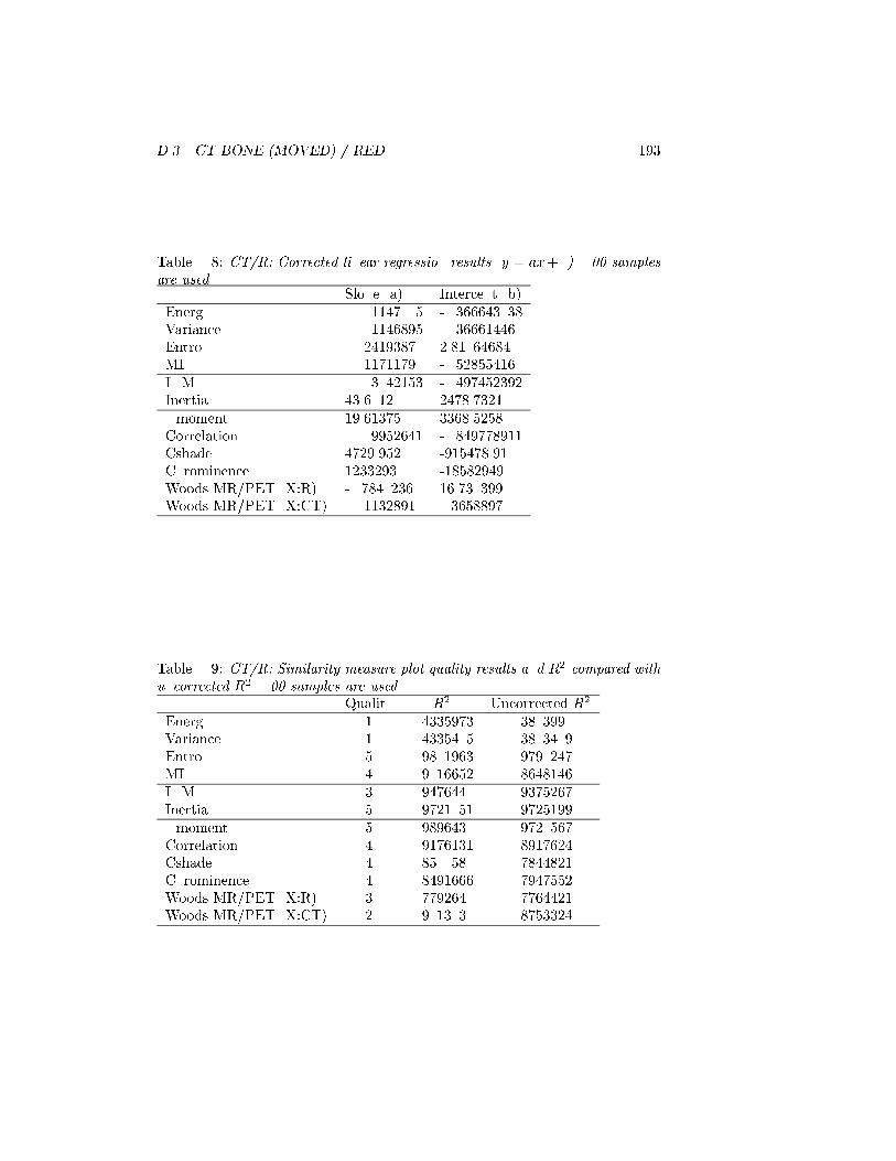
D.3. CT BONE (MOVED) / RED 193
Table D.8: CT/R: Corrected linear regression results (y = ax+ b). 500 samplesare used.
Slope (a) Intercept (b)Energy 0.001147005 -0.366643038Variance 0.001146895 -0.366614460Entropy 0.02419387 2.81064684MI 0.01171179 -0.52855416IDM 0.003042153 -0.497452392Inertia 43.6012 2478.7321Dmoment 19.61375 3368.52580Correlation 0.009952641 -0.849778911Cshade 4729.952 -915478.910Cprominence 1233293 -185829490Woods MR/PET (X:R) -0.7840236 16.7303990Woods MR/PET (X:CT) 0.01132891 0.36588970
Table D.9: CT/R: Similarity measure plot quality results and R2 compared withuncorrected R2. 500 samples are used.
Quality R2 Uncorrected R2
Energy 1 0.4335973 0.3803990Variance 1 0.4335405 0.3803409Entropy 5 0.9801963 0.9790247MI 4 0.9016652 0.8648146IDM 3 0.9476440 0.9375267Inertia 5 0.9721051 0.9725199Dmoment 5 0.9896430 0.9720567Correlation 4 0.9176131 0.8917624Cshade 4 0.8500580 0.7844821Cprominence 4 0.8491666 0.7947552Woods MR/PET (X:R) 3 0.7792640 0.7764421Woods MR/PET (X:CT) 2 0.9013030 0.8753324

194 APPENDIX D. GLCM PLOTS
-0.375
-0.37
-0.365
-0.36
-0.355
-0.35
-0.345
-0.34
-0.335
-0.33
0 2 4 6 8 10 12 14 16
’ctr_s2_dist_rot.energy’
-0.39
-0.38
-0.37
-0.36
-0.35
-0.34
-0.33
-0.32
0 2 4 6 8 10 12 14 16
’ctr_s2_dist_tr.energy’
-0.375
-0.37
-0.365
-0.36
-0.355
-0.35
-0.345
-0.34
-0.335
0 2 4 6 8 10 12 14 16
’ctr_s2_dist.energy’
-0.375
-0.37
-0.365
-0.36
-0.355
-0.35
-0.345
-0.34
-0.335
0 2 4 6 8 10 12 14
’ctr_s2_dist.energyC’
Figure D.49: CT/R: Distance/energy: Rotation only, Translation only, Normaland Corrected.

D.3. CT BONE (MOVED) / RED 195
-0.375
-0.37
-0.365
-0.36
-0.355
-0.35
-0.345
-0.34
-0.335
-0.33
0 2 4 6 8 10 12 14 16
’ctr_s2_dist_rot.variance’
-0.39
-0.38
-0.37
-0.36
-0.35
-0.34
-0.33
-0.32
0 2 4 6 8 10 12 14 16
’ctr_s2_dist_tr.variance’
-0.375
-0.37
-0.365
-0.36
-0.355
-0.35
-0.345
-0.34
-0.335
0 2 4 6 8 10 12 14 16
’ctr_s2_dist.variance’
-0.375
-0.37
-0.365
-0.36
-0.355
-0.35
-0.345
-0.34
-0.335
0 2 4 6 8 10 12 14
’ctr_s2_dist.varianceC’
Figure D.50: CT/R: Distance/variance: Rotation only, Translation only, Nor-mal and Corrected.
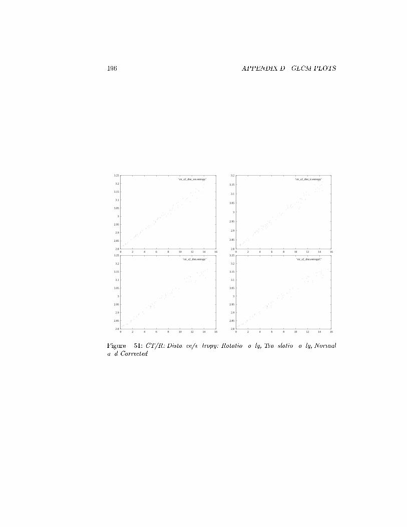
196 APPENDIX D. GLCM PLOTS
2.8
2.85
2.9
2.95
3
3.05
3.1
3.15
3.2
3.25
0 2 4 6 8 10 12 14 16
’ctr_s2_dist_rot.entropy’
2.8
2.85
2.9
2.95
3
3.05
3.1
3.15
3.2
0 2 4 6 8 10 12 14 16
’ctr_s2_dist_tr.entropy’
2.8
2.85
2.9
2.95
3
3.05
3.1
3.15
3.2
3.25
0 2 4 6 8 10 12 14 16
’ctr_s2_dist.entropy’
2.8
2.85
2.9
2.95
3
3.05
3.1
3.15
3.2
3.25
0 2 4 6 8 10 12 14 16
’ctr_s2_dist.entropyC’
Figure D.51: CT/R: Distance/entropy: Rotation only, Translation only, Normaland Corrected.

D.3. CT BONE (MOVED) / RED 197
-0.54
-0.52
-0.5
-0.48
-0.46
-0.44
-0.42
-0.4
0 2 4 6 8 10 12 14 16
’ctr_s2_dist_rot.mi’
-0.54
-0.52
-0.5
-0.48
-0.46
-0.44
-0.42
-0.4
-0.38
-0.36
-0.34
0 2 4 6 8 10 12 14 16
’ctr_s2_dist_tr.mi’
-0.54
-0.52
-0.5
-0.48
-0.46
-0.44
-0.42
-0.4
-0.38
-0.36
-0.34
0 2 4 6 8 10 12 14 16
’ctr_s2_dist.mi’
-0.54
-0.52
-0.5
-0.48
-0.46
-0.44
-0.42
-0.4
-0.38
-0.36
-0.34
0 2 4 6 8 10 12 14
’ctr_s2_dist.miC’
Figure D.52: CT/R: Distance/MI: Rotation only, Translation only, Normal andCorrected.

198 APPENDIX D. GLCM PLOTS
-0.5
-0.49
-0.48
-0.47
-0.46
-0.45
-0.44
-0.43
0 2 4 6 8 10 12 14 16
’ctr_s2_dist_rot.idm’
-0.5
-0.49
-0.48
-0.47
-0.46
-0.45
-0.44
-0.43
0 2 4 6 8 10 12 14 16
’ctr_s2_dist_tr.idm’
-0.5
-0.49
-0.48
-0.47
-0.46
-0.45
-0.44
-0.43
0 2 4 6 8 10 12 14 16
’ctr_s2_dist.idm’
-0.5
-0.49
-0.48
-0.47
-0.46
-0.45
-0.44
-0.43
0 2 4 6 8 10 12 14 16 18
’ctr_s2_dist.idmC’
Figure D.53: CT/R: Distance/IDM: Rotation only, Translation only, Normaland Corrected.
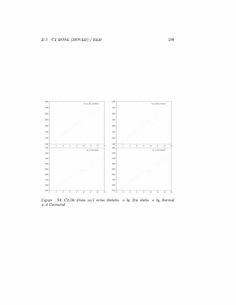
D.3. CT BONE (MOVED) / RED 199
2500
2600
2700
2800
2900
3000
3100
3200
0 2 4 6 8 10 12 14 16
’ctr_s2_dist_rot.inertia’
2500
2600
2700
2800
2900
3000
3100
3200
0 2 4 6 8 10 12 14 16
’ctr_s2_dist_tr.inertia’
2500
2600
2700
2800
2900
3000
3100
3200
3300
0 2 4 6 8 10 12 14 16
’ctr_s2_dist.inertia’
2500
2600
2700
2800
2900
3000
3100
3200
3300
0 2 4 6 8 10 12 14 16
’ctr_s2_dist.inertiaC’
Figure D.54: CT/R: Distance/inertia: Rotation only, Translation only, Normaland Corrected.

200 APPENDIX D. GLCM PLOTS
3350
3400
3450
3500
3550
3600
3650
3700
3750
3800
0 2 4 6 8 10 12 14 16
’ctr_s2_dist_rot.dmoment’
3350
3400
3450
3500
3550
3600
3650
3700
3750
0 2 4 6 8 10 12 14 16
’ctr_s2_dist_tr.dmoment’
3350
3400
3450
3500
3550
3600
3650
3700
3750
3800
0 2 4 6 8 10 12 14 16
’ctr_s2_dist.dmoment’
3350
3400
3450
3500
3550
3600
3650
3700
3750
3800
0 2 4 6 8 10 12 14 16 18 20
’ctr_s2_dist.dmomentC’
Figure D.55: CT/R: Distance/Dmoment: Rotation only, Translation only, Nor-mal and Corrected.
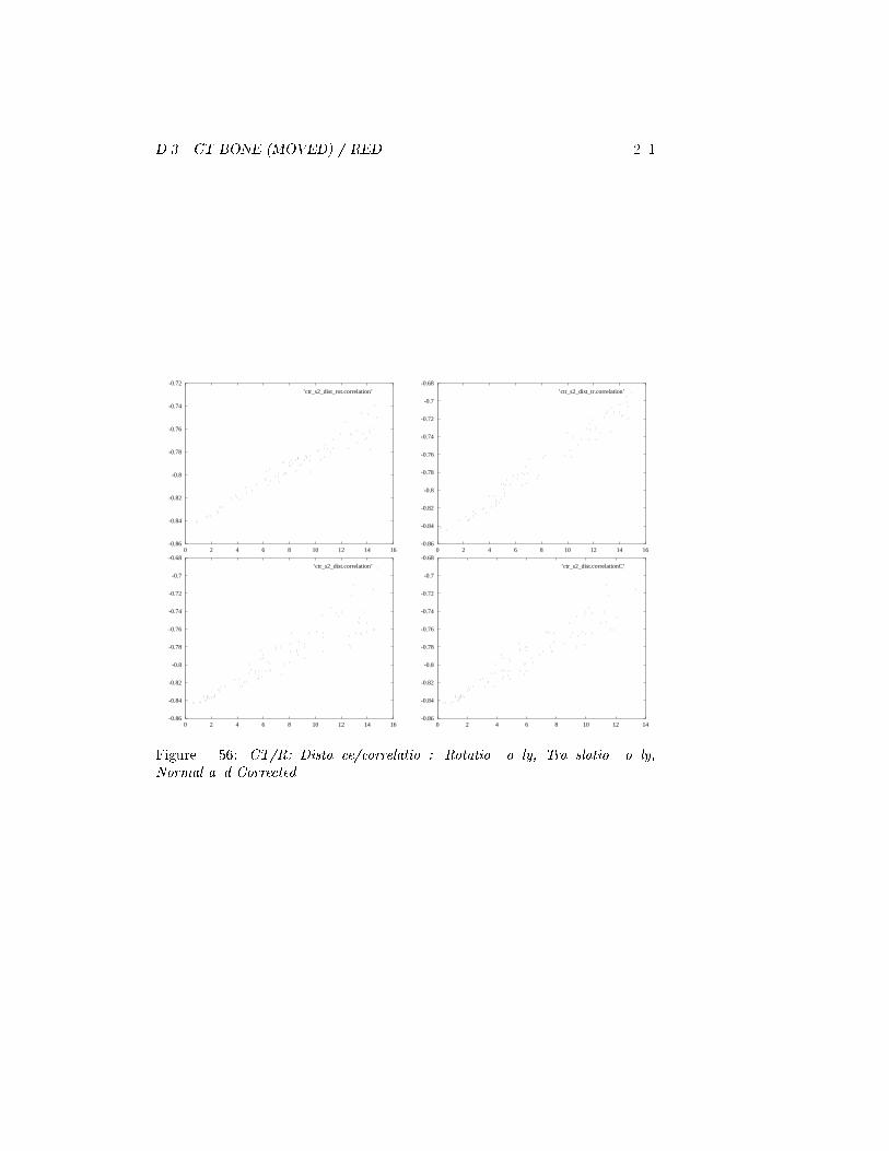
D.3. CT BONE (MOVED) / RED 201
-0.86
-0.84
-0.82
-0.8
-0.78
-0.76
-0.74
-0.72
0 2 4 6 8 10 12 14 16
’ctr_s2_dist_rot.correlation’
-0.86
-0.84
-0.82
-0.8
-0.78
-0.76
-0.74
-0.72
-0.7
-0.68
0 2 4 6 8 10 12 14 16
’ctr_s2_dist_tr.correlation’
-0.86
-0.84
-0.82
-0.8
-0.78
-0.76
-0.74
-0.72
-0.7
-0.68
0 2 4 6 8 10 12 14 16
’ctr_s2_dist.correlation’
-0.86
-0.84
-0.82
-0.8
-0.78
-0.76
-0.74
-0.72
-0.7
-0.68
0 2 4 6 8 10 12 14
’ctr_s2_dist.correlationC’
Figure D.56: CT/R: Distance/correlation: Rotation only, Translation only,Normal and Corrected.
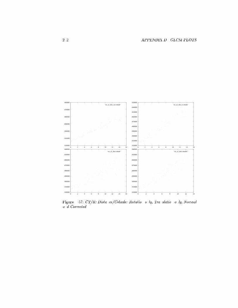
202 APPENDIX D. GLCM PLOTS
-920000
-910000
-900000
-890000
-880000
-870000
-860000
0 2 4 6 8 10 12 14 16
’ctr_s2_dist_rot.cshade’
-920000
-910000
-900000
-890000
-880000
-870000
-860000
-850000
-840000
-830000
0 2 4 6 8 10 12 14 16
’ctr_s2_dist_tr.cshade’
-920000
-910000
-900000
-890000
-880000
-870000
-860000
-850000
-840000
0 2 4 6 8 10 12 14 16
’ctr_s2_dist.cshade’
-920000
-910000
-900000
-890000
-880000
-870000
-860000
-850000
-840000
0 2 4 6 8 10 12 14
’ctr_s2_dist.cshadeC’
Figure D.57: CT/R: Distance/Cshade: Rotation only, Translation only, Normaland Corrected.

D.3. CT BONE (MOVED) / RED 203
-1.88e+08
-1.86e+08
-1.84e+08
-1.82e+08
-1.8e+08
-1.78e+08
-1.76e+08
-1.74e+08
-1.72e+08
0 2 4 6 8 10 12 14 16
’ctr_s2_dist_rot.cprominence’
-1.9e+08
-1.85e+08
-1.8e+08
-1.75e+08
-1.7e+08
-1.65e+08
-1.6e+08
0 2 4 6 8 10 12 14 16
’ctr_s2_dist_tr.cprominence’
-1.9e+08
-1.85e+08
-1.8e+08
-1.75e+08
-1.7e+08
-1.65e+08
0 2 4 6 8 10 12 14 16
’ctr_s2_dist.cprominence’
-1.9e+08
-1.85e+08
-1.8e+08
-1.75e+08
-1.7e+08
-1.65e+08
0 2 4 6 8 10 12 14
’ctr_s2_dist.cprominenceC’
Figure D.58: CT/R: Distance/Cprominence: Rotation only, Translation only,Normal and Corrected.
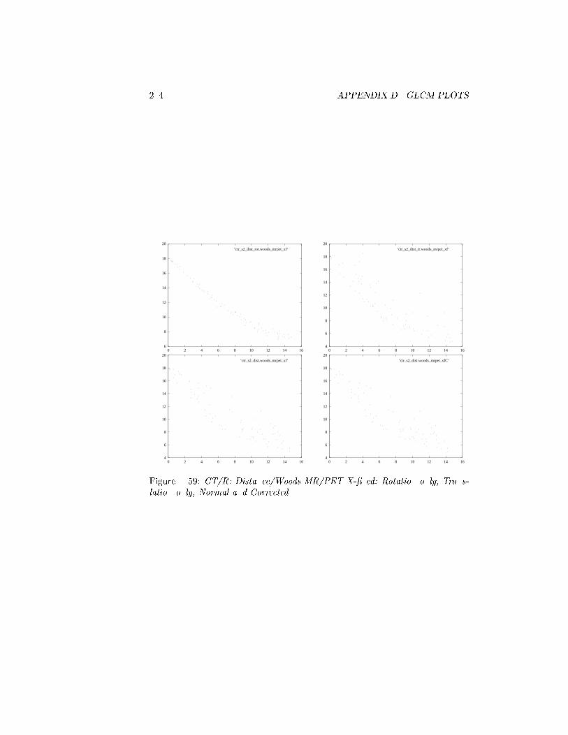
204 APPENDIX D. GLCM PLOTS
6
8
10
12
14
16
18
20
0 2 4 6 8 10 12 14 16
’ctr_s2_dist_rot.woods_mrpet_xf’
4
6
8
10
12
14
16
18
20
0 2 4 6 8 10 12 14 16
’ctr_s2_dist_tr.woods_mrpet_xf’
4
6
8
10
12
14
16
18
20
0 2 4 6 8 10 12 14 16
’ctr_s2_dist.woods_mrpet_xf’
4
6
8
10
12
14
16
18
20
0 2 4 6 8 10 12 14 16
’ctr_s2_dist.woods_mrpet_xfC’
Figure D.59: CT/R: Distance/Woods MR/PET X-xed: Rotation only, Trans-lation only, Normal and Corrected.

D.3. CT BONE (MOVED) / RED 205
0.36
0.38
0.4
0.42
0.44
0.46
0.48
0.5
0 2 4 6 8 10 12 14 16
’ctr_s2_dist_rot.woods_mrpet_xm’
0.36
0.38
0.4
0.42
0.44
0.46
0.48
0.5
0.52
0.54
0.56
0 2 4 6 8 10 12 14 16
’ctr_s2_dist_tr.woods_mrpet_xm’
0.36
0.38
0.4
0.42
0.44
0.46
0.48
0.5
0.52
0.54
0.56
0 2 4 6 8 10 12 14 16
’ctr_s2_dist.woods_mrpet_xm’
0.36
0.38
0.4
0.42
0.44
0.46
0.48
0.5
0.52
0.54
0.56
0 2 4 6 8 10 12 14
’ctr_s2_dist.woods_mrpet_xmC’
Figure D.60: CT/R: Distance/Woods MR/PET X-moved: Rotation only,Translation only, Normal and Corrected.
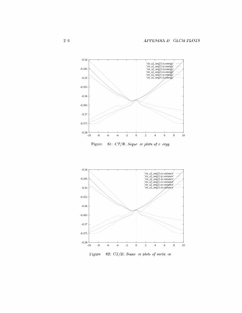
206 APPENDIX D. GLCM PLOTS
-0.38
-0.375
-0.37
-0.365
-0.36
-0.355
-0.35
-0.345
-0.34
-10 -8 -6 -4 -2 0 2 4 6 8 10
’ctr_s2_seq21.tx.energy’’ctr_s2_seq21.ty.energy’’ctr_s2_seq21.tz.energy’’ctr_s2_seq21.rx.energy’’ctr_s2_seq21.ry.energy’’ctr_s2_seq21.rz.energy’
Figure D.61: CT/R: Sequence plots of energy.
-0.38
-0.375
-0.37
-0.365
-0.36
-0.355
-0.35
-0.345
-0.34
-10 -8 -6 -4 -2 0 2 4 6 8 10
’ctr_s2_seq21.tx.variance’’ctr_s2_seq21.ty.variance’’ctr_s2_seq21.tz.variance’’ctr_s2_seq21.rx.variance’’ctr_s2_seq21.ry.variance’’ctr_s2_seq21.rz.variance’
Figure D.62: CT/R: Sequence plots of variance.
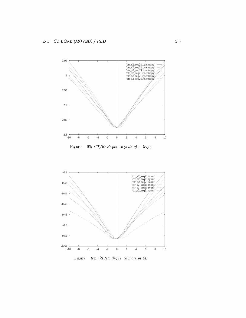
D.3. CT BONE (MOVED) / RED 207
2.8
2.85
2.9
2.95
3
3.05
-10 -8 -6 -4 -2 0 2 4 6 8 10
’ctr_s2_seq21.tx.entropy’’ctr_s2_seq21.ty.entropy’’ctr_s2_seq21.tz.entropy’’ctr_s2_seq21.rx.entropy’’ctr_s2_seq21.ry.entropy’’ctr_s2_seq21.rz.entropy’
Figure D.63: CT/R: Sequence plots of entropy.
-0.54
-0.52
-0.5
-0.48
-0.46
-0.44
-0.42
-0.4
-10 -8 -6 -4 -2 0 2 4 6 8 10
’ctr_s2_seq21.tx.mi’’ctr_s2_seq21.ty.mi’’ctr_s2_seq21.tz.mi’’ctr_s2_seq21.rx.mi’’ctr_s2_seq21.ry.mi’’ctr_s2_seq21.rz.mi’
Figure D.64: CT/R: Sequence plots of MI.
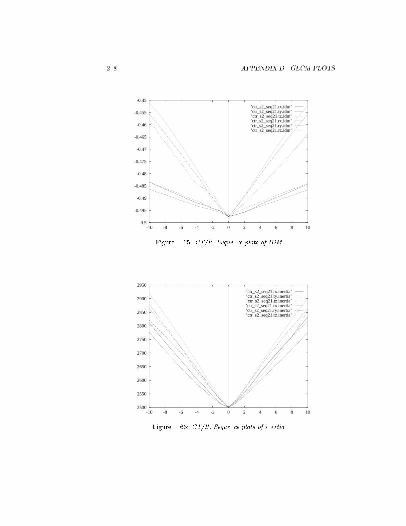
208 APPENDIX D. GLCM PLOTS
-0.5
-0.495
-0.49
-0.485
-0.48
-0.475
-0.47
-0.465
-0.46
-0.455
-0.45
-10 -8 -6 -4 -2 0 2 4 6 8 10
’ctr_s2_seq21.tx.idm’’ctr_s2_seq21.ty.idm’’ctr_s2_seq21.tz.idm’’ctr_s2_seq21.rx.idm’’ctr_s2_seq21.ry.idm’’ctr_s2_seq21.rz.idm’
Figure D.65: CT/R: Sequence plots of IDM.
2500
2550
2600
2650
2700
2750
2800
2850
2900
2950
-10 -8 -6 -4 -2 0 2 4 6 8 10
’ctr_s2_seq21.tx.inertia’’ctr_s2_seq21.ty.inertia’’ctr_s2_seq21.tz.inertia’’ctr_s2_seq21.rx.inertia’’ctr_s2_seq21.ry.inertia’’ctr_s2_seq21.rz.inertia’
Figure D.66: CT/R: Sequence plots of inertia.
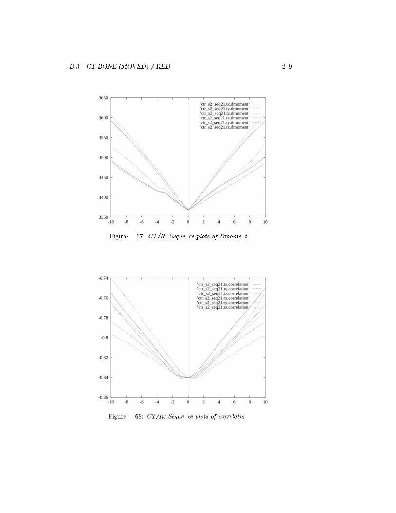
D.3. CT BONE (MOVED) / RED 209
3350
3400
3450
3500
3550
3600
3650
-10 -8 -6 -4 -2 0 2 4 6 8 10
’ctr_s2_seq21.tx.dmoment’’ctr_s2_seq21.ty.dmoment’’ctr_s2_seq21.tz.dmoment’’ctr_s2_seq21.rx.dmoment’’ctr_s2_seq21.ry.dmoment’’ctr_s2_seq21.rz.dmoment’
Figure D.67: CT/R: Sequence plots of Dmoment.
-0.86
-0.84
-0.82
-0.8
-0.78
-0.76
-0.74
-10 -8 -6 -4 -2 0 2 4 6 8 10
’ctr_s2_seq21.tx.correlation’’ctr_s2_seq21.ty.correlation’’ctr_s2_seq21.tz.correlation’’ctr_s2_seq21.rx.correlation’’ctr_s2_seq21.ry.correlation’’ctr_s2_seq21.rz.correlation’
Figure D.68: CT/R: Sequence plots of correlation.
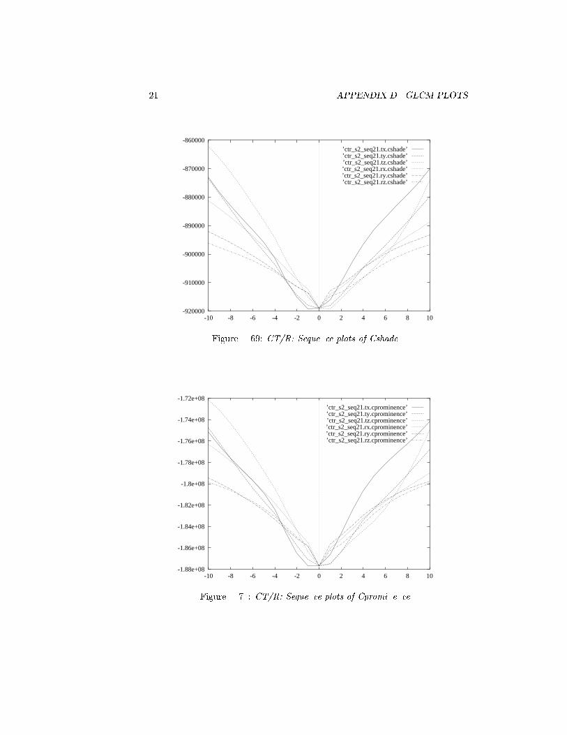
210 APPENDIX D. GLCM PLOTS
-920000
-910000
-900000
-890000
-880000
-870000
-860000
-10 -8 -6 -4 -2 0 2 4 6 8 10
’ctr_s2_seq21.tx.cshade’’ctr_s2_seq21.ty.cshade’’ctr_s2_seq21.tz.cshade’’ctr_s2_seq21.rx.cshade’’ctr_s2_seq21.ry.cshade’’ctr_s2_seq21.rz.cshade’
Figure D.69: CT/R: Sequence plots of Cshade.
-1.88e+08
-1.86e+08
-1.84e+08
-1.82e+08
-1.8e+08
-1.78e+08
-1.76e+08
-1.74e+08
-1.72e+08
-10 -8 -6 -4 -2 0 2 4 6 8 10
’ctr_s2_seq21.tx.cprominence’’ctr_s2_seq21.ty.cprominence’’ctr_s2_seq21.tz.cprominence’’ctr_s2_seq21.rx.cprominence’’ctr_s2_seq21.ry.cprominence’’ctr_s2_seq21.rz.cprominence’
Figure D.70: CT/R: Sequence plots of Cprominence.
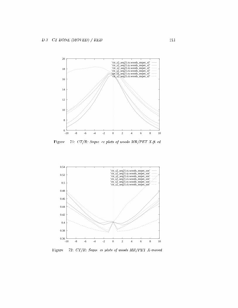
D.3. CT BONE (MOVED) / RED 211
6
8
10
12
14
16
18
20
-10 -8 -6 -4 -2 0 2 4 6 8 10
’ctr_s2_seq21.tx.woods_mrpet_xf’’ctr_s2_seq21.ty.woods_mrpet_xf’’ctr_s2_seq21.tz.woods_mrpet_xf’’ctr_s2_seq21.rx.woods_mrpet_xf’’ctr_s2_seq21.ry.woods_mrpet_xf’’ctr_s2_seq21.rz.woods_mrpet_xf’
Figure D.71: CT/R: Sequence plots of woods MR/PET X-xed.
0.36
0.38
0.4
0.42
0.44
0.46
0.48
0.5
0.52
0.54
-10 -8 -6 -4 -2 0 2 4 6 8 10
’ctr_s2_seq21.tx.woods_mrpet_xm’’ctr_s2_seq21.ty.woods_mrpet_xm’’ctr_s2_seq21.tz.woods_mrpet_xm’’ctr_s2_seq21.rx.woods_mrpet_xm’’ctr_s2_seq21.ry.woods_mrpet_xm’’ctr_s2_seq21.rz.woods_mrpet_xm’
Figure D.72: CT/R: Sequence plots of woods MR/PET X-moved.

212 APPENDIX D. GLCM PLOTS

Bibliography
[Alp90] N.M. Alpert, J.F. Bradshaw, D. Kennedy, and J.A. Correia, The prin-cipal axes transformation - A method for image registration, J. Nucl.Med., 31:1717-1722, 1990
[Ami91] Y. Amit, U. Grenander, and M. Piccioni, Structural image restorationthrough deformable templates, J. Am. Stat. Ass., 86(414):376-387, 1991
[Api87] A. Apicella, J.S. Kippenham, and J.H. Nagel, Fast multi-modality im-age matching, IEEE Trans. on Pattern Analysis and Machine Intelli-gence, 9:698-700, 1987
[Ara92] L.K. Arata and A.P. Dhawan, Iterative principal axes registration: Anew algorithm for retrospective correlation of MR-PET brain images,Proc. Annu. Int. Conf. IEEE Eng. Med. Biol. Soc., 14:2776-2778, 1992
[Aru87] K.S. Arun, T.S. Huang, and S.D. Blostein, Least-squares tting of two3-D point sets, IEEE Trans. Pattern Analysis and Machine Intelligence,9:998-700, 1987
[Baj88] R. Bajcsy, M. Reivich, and S. Kovacic, Evaluation of registration ofPET images and CT images, Tech. Rep. ms-cis-88-89, grasp lab 163,Depart. of Computer and Information Science, School of Engineeringand Applied Science, Univ. of Pennsylvania, 1988
[Baj89] R. Bajcsy and S. Kovacic, Multiresolution elastic matching, ComputerVision, Graphics and Image Processing, 46:1-21, 1989
[Brt95] R. Barret et al., Templates for the solution of linearsystems: Building blocks for iterative methods, WWWhttp://www.netlib.org/templates/templates.ps, 1995
[Brw77] H.G. Barrow, J.M. Tenembaum, R.C. Bolles, and H.C. Wolf, Paramet-ric correspondence and chamfer matching, Proc. 5th Int. Joint Conf.on Articial Intelligence, Cambridge, MA, pp. 659-663, 1977
[Bar94] K.A. Bartels, A.C. Bovik and C.E. Grin, Spatio-temporal trackingof material shape change via multi-dimensional splines, Proc. IEEEWorkshop Biomedical Image Analysis, Seattle, USA, pp. 110-116, June1994
213

214 BIBLIOGRAPHY
[Beg88] D. Begis, C. Delpuech, P. le Tallec, L. Loth, and M. Vidrascu, A nite-element model of tracheal collapse, the American Physiology Society,pp. 1359-1368, 1988
[Bes92] P.J. Besl and N.D. McKay, A methods for registration of 3-D shapes,IEEE Trans. Pattern Analysis and Machine Intelligence, 14(2):239256,1992
[Bj61] A. Bjork, The relationship of the jaws to the cranium, in A. Lundstrom,Introduction to orthodontics, McGraw-Hill, London, 1961
[Bj63] A. Bjork, Variations in the growth pattern of the human mandible:Longitudinal radiographic study by the implant method, J. Dent. Res.,42:400, 1963
[Bj69] A. Bjork, Prediction of mandibular growth rotation, Am. J. Ortho.,55:585, 1969
[Bj72] A. Bjork and V. Skieller, Facial development and tooth eruption, Am.J. Ortho., 62:339, 1972
[Bj77] A. Bjork and V. Skieller, Growth of the maxilla in three dimensions asrevealed radiographically by the implant method, Brit. J. Ortho., 4:53,1977
[Boe90] R. Boesecke, T. Bruckner, and G. Ende, Landmark based correlationof medical images, Phys. Med. Biol., 35(1):121-126, 1990
[Boo89] F.L. Bookstein, Principal warps: Thin-plate splines and the decom-position of deformations, IEEE Trans. Pattern Analysis and MachineIntelligence, 11:567-585, 1989
[Boo92] F.L. Bookstein and W.D.K. Green, Edge information at landmarks inmedical images, Proc. SPIE 1808: Visualization in Biomedical Com-puting, pp. 242-258, 1992
[Bor88] G. Borgefors, Hierarchical chamfer matching: A paramteric edgematching algorithm, IEEE Trans. Pattern Analysis and Machine In-telligence, 10:849-865, 1988
[BN94] M. Bro-Nielsen, Active nets and cubes, IMM Tech. Rep., 1994
[BN95] M. Bro-Nielsen, Modelling elasticity in solids using Active Cubes - Ap-plication to simulated operations, Proc. Computer Vision, Virtual Re-ality and Robotics in Medicine (CVRMed'95), pp. 535-541, 1995
[BN95b] M. Bro-Nielsen and S. Cotin, Soft tissue modelling in surgery simula-tion for prediction of results of craniofacial operations & steps towardsvirtual reality training systems, Proc. 3rd Int. Workshop on Rapid Pro-totyping in Medicine & Computer-Assisted Surgery, 1995
BIBLIOGRAPHY 215
[BN96] M. Bro-Nielsen, Mvox: Interactive 2-4D medical image and graphicsvisualization software, Proc. Computer Assisted Radiology (CAR'96),1996
[BN96b] M. Bro-Nielsen, Mvox WWW homepage,http://www.imm.dtu.dk/ mvox/, 1996
[BN96c] M. Bro-Nielsen and S. Cotin, Real-time volumetric deformable mod-els for surgery simulation using nite elements and condensation, ac-cepted for Eurographics'96, 1996
[BN96d] M. Bro-Nielsen, Surgery simulation using fast nite elements, acceptedfor VBC'96, 1996
[BN96e] M. Bro-Nielsen and C. Gramkow, Fast uid registration of medicalimages, accepted for Visualization in Biomedical Imaging (VBC'96),1996
[Brt81] C. Broit, Optimal registration of deformed images, Doctoral disserta-tion, University of Pennsylvania, August 1981
[Bro92] L.G. Brown, A survey of image registration techniques, ACM Comput-ing Surveys, 24(4):325-376, 1992
[Bur81] D.J. Burr, A Dynamic model for image registration, Computer Vision,Graphics, and Image Processing, 15:102-112, 1981
[Cap93] L. Caponetti and A.M. Fanelli, Computer-aided simulation for bonesurgery, IEEE Computer Graphics & Applications, November, pp. 86-92, 1993
[Car86] G.F. Carey and J.T. Oden, Finite elements: Fluid mechanics VolumeVI, Prentice-Hall, New Jersey, ISBN 0-13-317132-9 025, 1986
[Che88] C-T. Chen, C.A. Pelizarri, G.T.Y. Chen, M.D. Cooper, and D.N.Levin, Image analysis of PET data with the aid of CT and MR images,Proc. Information Processing in Medical Imaging, pp. 601-611, 1988
[Che92] D.T. Chen and D. Zeltzer, Pump it up: Computer animation of abiomechanically based model of muscle using the nite element method,Computer Graphics, 26(2):89-98, 1992
[Chr93] G.E. Christensen, R.D. Rabbitt, and M.I. Miller, A deformable neu-roanatomy textbook based on viscous uid mechanics, Proc. Ann. Conf.Information Sciences and Systems, pp. 211-216, 1993
[Chr94] G.E. Christensen, M.I. Miller and M. Vannier, A 3D deformable mag-netic resonance textbook based on elasticity, in AAAI Spring Sympo-sium Series: Applications of Computer Vision in Medical Image Pro-cessing, pp. 153-156, Stanford University, March 1994
216 BIBLIOGRAPHY
[Chr94b] G.E. Christensen, R.D. Rabbitt and M.I. Miller, 3D brain mappingusing a deformable neuroanatomy, Physics in Medicine and Biology,39:609-618, 1994
[Chr94c] G.E. Christensen, Deformable shape models for anatomy, WashingtonUniversity Ph.D. Thesis, August 1994
[Chr96] G.E. Christensen, M.I. Miller, M. Vannier and U. Grenander, Individ-ualizing neuroanatomical atlases using a massively parallel computer,IEEE Computer, 29(1):32-38, January 1996
[Chr96b] G.E. Christensen, A.A. Kane, J.L. Marsh, and M. Vannier, A 3D de-formable infant atlas, Proc. Computer Assisted Radiology (CAR'96),pp. 847-852, 1996
[Cia87] P.G. Ciarlet, Mathematical elasticity Vol. 1: Three-dimensional elas-ticity, North-Holland, Amsterdam, ISBN 0-444-70259-8 (v. 1), 1987
[Coh89] L.D. Cohen and I. Cohen, Finite-element methods for active contourmodels and balloons for 2-D and 3-D images, IEEE Trans. PatternAnalysis and Machine Intelligence, 15(11):1131-1147, 1989
[Col93] A. Collignon, D. Vandermeulen, P. Suetens, G. Marchal, A. Baert, andA. Oosterlinck, Surface based registration of 3d medical images, Proc.SPIE Vol. 1898: Medical Imaging VII, 1993
[Col93b] A. Collignon, T. Geraud, D. Vandermeulen, P. Suetens, and G. Mar-chal, New high-performance 3d registration algorithms for 3d medicalimages, Proc. SPIE Vol. 1898: Image Processing, 779-788, 1993
[Col95] A. Collignon, D. Vandermeulen, P. Suetens, and G. Marchal, 3d multi-modality image registration using features space clustering, Proc. Com-puter Vision, Virtual Reality, and Robotics in Medicine (CVRMed'95),195-204, 1995
[Col95b] A. Collignon, F. Maes, D. Delaere, D. Vandermeulen, P. Suetens, andG. Marchal, Automated multi-modality image registration based on in-formation theory, Proc. Information Processing in Medical Imaging,263-274, 1995
[Cli92] D.L. Collins, T.M. Peters, W. Dai, A.C. Evans, Model-based segmen-tation of individual brain structures from MRI data, Proc. SPIE Visu-alization in Biomedical Computing (1808), pp. 10-23, 1992
[Cnr80] R.W. Conners and C.A. Harlow, A theoretical comparison of texturealgorithms, IEEE Trans. Pattern Analysis and Machine Intelligence,2(3):204-222, 1980
[Cnr84] R.W. Conners, M.M. Trivedi, and C.A. Harlow, Segmentation of ahigh-resolution urban scene using texture operators, Computer Vision,Graphics, and Image Processing, 25:273-310, 1984
BIBLIOGRAPHY 217
[Con84] K. Conradsen, En introduktion til statistik (Danish), IMM lecturenotes, 1984
[Coo95] T.F. Cootes , D.H. Cooper, C.J. Taylor and J. Graham, Active ShapeModels - Their training and application, Computer Vision Graphicsand Image Processing, 61:38-59, 1995
[Cot96] S. Cotin, H. Delingette, M. Bro-Nielsen, N. Ayache, J.M. Clement, V.Tassetti and J. Marescaux, Geometric and Physical representations fora simulator of hepatic surgery, Proc. Medicine Meets Virtual Reality,1996
[Cot96b] S. Cotin, H. Delingette, J.M. Clement, V. Tassetti, J. Marescaux, andN. Ayache, Volumetric deformable models for simulation of laparas-copic surgery, Proc. Computer Assisted Radiology (CAR'96), pp. 793-798, 1996
[Cov93] S.A. Cover, N.F. Ezquerra and J.F. O'Brien, R. Rowe, T. Gadacz andE. Palm, Interactively deformable models for surgery simulation, IEEEComputer Graphics & Applications, pp. 68-75, Nov. 1993
[Dav96] C. Davatzikos, Nonlinear registration of brain images using deformablemodels, Proc. IEEE Workshop on Mathematical Methods in Biomedi-cal Image Analysis, 1996
[Dav96b] C. Davatzikos, Spatial normalization of 3d brain images using defor-mable models, Submitted Journal of Computer Assisted Tomography,1996
[Dec95] J. Declerck, G. Subsol, J-P. Thirion, and N. Ayache, Automatic re-trieval of anatomical structures in 3D medical images, Proc. ComputerVision, Virtual Reality and Robotics in Medicine (CVRMed'95), pp;153-162, 1995
[Dec96] J. Declerck, J. Feldmar, M.L. Goris, and F. Betting. Automatic regis-tration and alignment on a template of cardiac stress & rest SPECTimages, INRIA Tech. Rep. 2770, 1996
[Del94] H. Delingette, G. Subsol, S. Cotin and J. Pignon, A craniofacialsurgery simulation testbed, INRIA Tech. Rep. 2199, 1994
[Del94b] H. Delingette, Simplex Meshes: a general representation for 3Dshape reconstruction, Proc. Computer Vision and Pattern Recognition(CVPR'94), 1994
[Deu95] O. Deussen, L. Kobbelt, and P. Tucke, Using simulated annealing toobtain good approximations of deformable bodies, Proc. EuroGraphicsWorkshop on Animation and Simulation, 1995
218 BIBLIOGRAPHY
[Doc76] M.P. Do Carmo, Dierential geometry of curves and surfaces, USA,Prentice-Hall, 1976
[Du73] R.O. Duda and P.E. Hart, Pattern classication and scene anal-ysis, Stanford Research Institute, Menlo Park, CA, USA, Wiley-Interscience, 1973
[Els91] P.A. van den Elsen, and M.A. Viergever,Marker guided registration ofelectromagnetic dipole data with tomographic images, Proc. Informa-tion Processing in Medical Imaging, pp. 142-153, 1991
[Els92] P.A. van den Elsen, J.B.A. Maintz, E-J.D. Pol, and M.A. Viergever,Image fusion using geometrical features, Proc. SPIE Vol. 1808: Visu-alization in Biomedical Computing, 172-186, 1992
[Els93] P.A. van den Elsen, E-J.D. Pol, and M.A. Viergever, Medical imagematching: A review with classication, IEEE Eng. Med. Biol., 12:26-39, 1993
[Els94] P.A. van den Elsen, Retrospective fusion of CT and MR brain imagesusing mathematical operators, AAAI Spring Symposium Series: Appli-cations of Computer Vision in Medical Image Processing, 30-33, 1994
[Els94b] P.A. van den Elsen, T.S. Sumanaweera, P.F. Hemler, S. Napel, andJ. Adler, Grey value correlation techniques used for automatic match-ing of CT and MR brain and spine images, Proc. SPIE Vol. 2359:Visualization in Biomedical Computing, 227-237, 1994
[Els95] P.A. van den Elsen, J.B.A. Maintz, E-J.D. Pol, and M.A. Viergever,Automatic registration of CT and MR brain images using correlation ofgeometrical features, IEEE Trans. on Medical Imaging, 14(2):384-396,1995
[Eva88] A.C. Evans, C. Beil, S. Marret, C.J. Thompson, and A. Hakim,Anatomical-functional correlation using an adjustable mri-based regionof interest atlas with positron emission tomography, J. Cerebral BloodFlow and Metabolism, 8:513-530, 1988
[Eva91] A.C. Evans, W. Dai, L. Collins, P. Neelin, S. Marret, Warping of acomputerized 3-D atlas to match brain image volumes for quantitativeneuroanatomical and functional analysis, Proc. SPIE Medical ImagingV (1445), pp. 236-246, 1991
[Eva92] A.C. Evans, S. Marret, P. Neelin, D.L. Collins, K. Worsley, W. Dai,S. Milot, E. Meyer, and D. Bub, Anatomical mapping of functionalactivation in stereotactic coordinate space, Neuroimage, 1:43-53, 1992
[Fab88] T.L. Faber and E.M. Stokely, Orientation of 3-D structures in med-ical images, IEEE Trans. Pattern Analysis and Machine Intelligence,10:626-633, 1988

BIBLIOGRAPHY 219
[Fau86] O.D. Faugeras and M. Hebert, The representation, recognition, andlocation of 3-D objects, Int. J. Robotics Research, 5:27-52, 1986
[Fel94] J. Feldmar and N. Ayache, Rigid, ane, and locally ane registrationof free-form surfaces, Int. J. of Computer Vision, in press, also INRIATech. Rep. 2220, 1996
[Fid94] M. Fidrich and J-P. Thirion, Multiscale extraction and representationof features from medical images, INRIA Tech. Rep. 2365, 1994
[Fox85] P.T. Fox, J.S. Perlmutter, and M.E. Raichle, A stereotactic method ofanatomical localization for positron emission tomography, J. ComputerAssisted Tomography, 9(1):141-153, 1985
[GA86] A. Gamboa-Aldeco and G.T.Y. Chen, Correlation of 3D surfaces frommultiple modalities in medical imaging, Proc. SPIE 626: MedicineXIV/PACS IV, pp. 467-473, 1986
[Ge92] Y. Ge, J.R. Votaw, R.A. Margolin, J.M. Fitzpatrick, R.J. Maciunas,and R.M. Kessler, Reformatting PET images by tting of the propor-tional grid system: Implementation anbd validation, Proc. SPIE 1652:Medical Imaging VI: Image Processing, pp. 397-408, 1992
[Gee93] J.C. Gee, M. Reivich and R. Bajcsy, Elastically deforming atlas tomatch anatomical brain images, Journal of Computer Assisted Tomog-raphy, 17(2):225-236, March 1993
[Gei93] B. Geiger, Three-dimensional modeling of human organs and its ap-plication to diagnosis and surgical planning, INRIA Tech. Rep. 2105,Dec. 1993
[Gib95] S.F. Frisken Gibson, Beyond volume rendering: Visualization, hapticexploration, and physical modeling of voxel-based objects, Proc. Euro-Graphics Workshop on Visualization in Scientic Computing, 1995
[Goo82] D.H. Goose and J. Appleton, Human dentofacial growth, PergamonPress, ISBN 0-08-026393-3, 1982
[Gou89] J-P. Gourret, N.M. Thalmann and D. Thalmann, Simulation of objectand human skin deformations in a grasping task, 23(3):21-30, 1989
[Gra96] C. Gramkow, Registration of 2D and 3D medical images, M.Sc. the-sis, Department of Mathematical Modelling, Technical University ofDenmark (IMM/DTU), 1996
[Gre91] Greitz, Bohm, Holte, and Eriksson, A computerized brain atlas: Con-struction, anatomical content, and some applications, J. Computer As-sisted Tomography, 15(1):26-38, 1991
220 BIBLIOGRAPHY
[Gue92] A. Gueziec and N. Ayache, Smoothing and matching of 3-D spacecurves, Proc. SPIE 1808: Visualization in Biomedical Imaging, pp.259-273, 1992
[Har73] R.M. Haralick, K. Shanmugan, and I. Dinstein, Textural features forimage classication, IEEE Trans. on Systems, Man, and Cybernetics,3:610-621, 1973
[Har79] R.M. Haralick, Statistical and structural approaches to texture, Proc.of the IEEE, 67(5):786-804, 1979
[Haw90] D.J. Hawkes, D.L.G. Hill, E.D. Lehmann, G.P. Robinson, M.N. Maiseyand A.C.F. Colchester, Preliminary work on the interpretation ofSPECT images with the aid of registered MR images and an MRderived 3D neuro-anatomical atlas, in K.H. Hohne, 3D Imaging inMedicine, NATO ASI series, Vol. F60, Springer-Verlag Berlin Heidel-berg, 1990
[Her94] M. van Herk and H.M. Kooy, Automatic three-dimensional correlationof CT-CT, CT-MRI, and CT-SPECT using chamfer matching, Med.Phys. 21(7):1163-1178, 1994
[HT95] HT Medical, http://www.ht.com, 1995
[Hi91] D.L.G. Hill, D.J. Hawkes, J.E. Crossman, M.J. Gleeson, T.C.S. Cox,E.E.C.M.L. Bracey, A.J. Strong, and P. Graves, Registration of MRand CT images for skull base surgery using point-like anatomical fea-tures, The British Journal of Radiology, 64:1030-1035, 1991
[Hi92] D.L.G. Hill, S.E.M. Green, J.E. Crossman, D.J. Hawkes, G.P. Robin-son, C.F. Ru, T.C.S. Cox, A.J. Strong, and M.J. Gleeson, Visuali-sation of multi-modal images for planning of skull base surgery, Proc.SPIE 1808: Visualization in Biomedical Computing, pp. 564-573, 1992
[Hi92b] D.L.G. Hill, D.J. Hawkes, Z. Hussain, S.E.M. Green, C.F. Ru, andG.P. Robinson, Accurate combination of CT and MR data of the head:Validation and applications in surgical and threapy planning, in C.Roux, G.T. Herman, and R. Collorec, 3D advanced image processingin medicine, pp. 79-83, 1992
[Hi93] D.L.G. Hill, Combination of 3D medical images from multiple modal-ities, Ph.D. thesis, University of London, 1993
[Hi93b] D.L.G. Hill, D.J. Hawkes, N. Harrison, and C.F. Ru, A strategy forautomated multimodality registration incorporating anatomical knowl-edge and imager characteristics, Proc. Information Processing in Med-ical Imaging, Lecture Notes in Computer Science 687, Springer-Verlag,Berlin, 182-196, 1993
BIBLIOGRAPHY 221
[Hi94] D.L.G. Hill and D.J. Hawkes, Medical image registration using knowl-edge of adjacency of anatomical structures, Image and Vision Comput-ing, 12:173-178, 1994
[Hi94b] D.L.G. Hill and D.J. Hawkes, Medical image registration using voxelsimilarity measures, AAAI Spring Symposium Series: Applications ofComputer Vision in Medical Image Processing, 34-37, 1994
[Hi94c] D.L.G. Hill, C. Studholme, and D.J. Hawkes, Voxel similarity measuresfor automated image registration, Proc. Visualization in BiomedicalComputing, 205-216, 1994
[Hoe92] K.H. Hohne, M. Bomans, M. Riemer, R. Schubert, U. Tiede and W.Lierse, A 3D anatomical atlas based on a volume model, IEEE Com-puter Graphics Applications, 12(4):72-78, 1992
[Hoe92b] K.H. Hohne, A. Pommert, M. Riemer, T. Schiemann, R. Schubert,and U. Tiede, Framework for the generation of 3d anatomical atlases,Proc. SPIE 1808: Visualization in Biomedical Computing, pp. 510-520,1992
[Hoe94] K.H. Hohne, A. Pommert, M. Riemer, T. Schiemann, R. Schubert, andU. Tiede, Representing spatial knowledge using the intelligent volumesconcept, Proc. Am. Ass. Art. Int., Spring Symposium: Applications ofComputer Vision in Medical Image Processing, 1994
[Hor87] B.K.P. Horn, Closed-form solution of absolute orientation using unitquaternions, J. Opt. Soc. Amer. A, 4:629-642, 1987
[Hor88] B.K.P. Horn, H.M. Hilden, and S. Negahdaripour, Closed-form solu-tion of absolute orientation using orthonormal matrices, J. Opt. Soc.Amer. A, 5:1127-1135, 1988
[Hue75] K.H. Huebner, The nite element method for engineers, John Wiley &Sons, ISBN 0-471-41950-8, 1975
[Jia92] H. Jiang, K.S. Holton, and R.A. Robb, Image registration of mul-timodality 3-D medical images by chamfer matching, Proc. SPIEVol. 1660: Biomedical Image Processing and Three-dimensional Mi-croscopy, 356-366, 1992
[Jia92b] H. Jiang, R.A. Robb, and K.S. Holton, A new approach to 3-d registra-tion of multimodality medical images by surface matching, Proc. SPIEVol. 1808: Visualization in Biomedical Computing, 196-213, 1992
[Kar87] H. Kardestuncer, Finite element handbook, McGraw-Hill, ISBN 0-07-033305-X, 1987
[Kas88] M. Kass, A. Witkin and D. Terzopoulos: Snakes: Active contour mod-els, Int. J. of Computer Vision, 2:321-331, 1988

222 BIBLIOGRAPHY
[Kee95] E. Keeve, S. Girod, P. Pfei e, and B. Girod, Interactive craniofacialsurgery planning by 3D-simulation and visualization, Proc. Int. Work-shop on Rapid Prototyping in Medicine & Computer-Assisted Surgery,1995
[Kee95b] E. Keeve, S. Girod, J. Jauch, and B. Girod, Anatomy-based model-ing of human facial tissue for craniofacial surgery simulation, Proc.Visualization'95 - Dynamics and Complexity, 1995
[Kee96] E. Keeve, S. Girod, P. Pfei e, and B. Girod, Anatomy-based facialtissue modeling using the nite element method, to appear Visualiza-tion'96, 1996
[Kee96b] E. Keeve, S. Girod, and B. Girod, Craniofacial surgery simulation, toappear Visualization in Biomedical Computing (VBC'96), 1996
[Kee96c] E. Keeve, S. Girod, and B. Girod, Computer-aided craniofacialsurgery, Proc. Computer Assisted Radiology (CAR'96), pp. 757-762,1996
[Ker96] J. Kerr, P. Ratiu, and M. Sellberg, Volume Renderingof Visible Human Data for an Anatomical Virtual En-vironment, Proc. Medicine Meets Virtual Reality IV, orhttp://www.eai.com/interactive/dhuman/paper/paper.html, 1996
[Koc96] R.M. Koch, M.H. Gross, F.R. Carls, D.F. von Buren, G. Fankhauser,and Y.I.H. Parish, Simulating facial surgery using nite element mod-els, to appear SIGGRAPH, 1996
[Ku96] C. Kuhn, U. Kuhnapfel, H.-G. Krumm, B. Neisius, A 'virtual reality'based training system for minimally invasive surgery, Proc. ComputerAssisted Radiology (CAR'96), pp. 764-769, 1996
[Kue93] U.G. Kuhnapfel, B. Neisius, H.G. Krumm, and M. Hubner, CAD-basedsimulation and modelling for endoscopic surgery, Endoscopic Surgery,1993
[Kue94] U.G. Kuhnapfel and B. Neisius, Realtime graphical computer simula-tion for endoscopic surgery, Proc. Medicine Meets Virtual Reality II,1994
[Kue95] U.G. Kuhnapfel, H. Krumm, C. Kuhn, M. Hubner, and B. Neisius,Endosurgery simulation with kismet, Proc. Virtual Reality World'95,1995
[Lee93] Y. Lee, D. Terzopoulos, and K. Waters, Constructing physical-basedfacial models of individuals, Proc. Graphics Interface'93, pp. 1-8, 1993
[Lee95] Y. Lee, D. Terzopoulos, and K. Waters, Realistic modeling of facialanimation, Proc. SIGGRAPH'95, 1995

BIBLIOGRAPHY 223
[Lem91] D. Lemoine, C. Barillot, B. Gibaud, and E. Pasqualini, An anatomical-based 3d registration system of multimodality and atlas data in neuro-surgery, Proc. Information Processing in Medical Imaging, pp. 154-164,1991
[Lev88] D.N. Levin, C.A. Pelizarri, G.T.Y. Chen, C-T. Chen and M.D. Cooper,Retrospective geometric correlation of MR, CT, and PET images, Ra-diology, 169:817-823, 1988
[Lin86] F.P.G.M. Linden, Facial growth and facial orthopedics, QuintessencePublishing Co., Chicago, 1986
[Lo94] L.J. Lo, J.L. Marsh, M.W. Vannier, and V.V. Patel, Craniofacialcomputer assisted surgical planning and simulation, Clin. Plast. Surg.,21:501-516, 1994
[Lor87] W.E. Lorensen and H. Cline, Marching Cubes: A high resolution 3Dsurface construction algorithm, Computer Graphics, 21(4):163-169,July 1987
[Mau93] C.R. Maurer and J.M. Fitzpatrick, A review of medical image regis-tration, in R.J. Maciunas, Interactive image-guided neurosurgery, ParkRidge, IL: American Association of Neurological Surgeons, 17-44, 1993
[McV85] E.R. McVeigh, R.M. Henkelman and M.J. Bronskill, Noise and ltra-tion in magnetic resonance imaging, Medical Physics, 12(5):586-591,1985
[Mil93] M.I. Miller, G.E. Christensen, Y. Amit and U. Grenander, Mathemati-cal textbok of deformable neuroanatomies, Proc. Natl. Acad. Sci. USA,90:11944-11948, December 1993
[Mon92] O. Monga, S. Benayoun, and O.D. Faugeras, From partial derivativesof 3D density images to ridge lines, Proc. SPIE 1808: Visualization inBiomedical Imaging, pp. 118-129, 1992
[Mos94] M. Moshfeghi, S. Ranganath, and K. Nawyn, Three-dimensional elas-tic matching of volumes, IEEE Trans. Image Processing, 3(2):128-138,1994
[Nie94] M. Nielsen, L. Florack and R. Deriche, Regularization and Scale Space,INRIA Tech. Rep. RR-2352, September 1994
[Nie96] M. Nielsen, R. Maas, W. Niessen, L. Florack, and B. ter Haar Romeny,Binocular stereo from grey-scale images, Submitted for Journal ofMathematical Imaging and Vision, 1996
[Nie96b] M. Nielsen, Personal communication, 1996

224 BIBLIOGRAPHY
[Pel89] C.A. Pelizarri, G.T.Y. Chen, D.R. Spelbring, R.R. Weichselbaumand C-T. Chen, Accurate three-dimensional registration of CT, PET,and/or MR images of the brain, Journal of Computer Asssisted To-mography, 13(1):20-26, 1989
[Pen96] X. Pennec and N. Ayache, Randomness and geometric features incomputer vision, INRIA Tech. Rep. 2820, short version submitted toCVPR'96, 1996
[Pet86] T.M. Peters, J.A. Clark, A. Olivier, E.P. Marchand, G. Mawko,M. Dieumegarde, L.V. Muresan and R. Ethier, Integrated stereotaxicimaging with CT, MR imaging, and digital subtraction angiography,Radiology, 161:821-826, 1986
[Pie92] S.D. Pieper, CAPS: Computer-aided plastic surgery, Ph.D. thesis,MIT, 1992
[Pie92b] S.D. Pieper, J. Rosen, and D. Zeltzer, Interactive graphics for plasticsurgery, Computer Graphics, 26(2):127-134, 1992
[Pok96] P. Pokrandt, Fast non-supervised matching: A probabilistic approach,Proc. Computer Assisted Radiology (CAR'96), pp. 306-310, 1996
[Pow64] M.J.D. Powell, An ecient method for nding the minimum of a func-tion of several variables without calculating derivatives, Comput. J.,7:155-163, 1964
[Num92] W.H. Press, S.A. Teukolsky, W.T. Vetterling, and B.P. Flannery, Nu-merical recipes in C, Cambridge University Press, 1992
[Rab95] R.D. Rabbitt, J.A. Weiss, G.E. Christensen and M.I. Miller, Mappingof hyperelastic deformable templates using the nite element method,Proc. SPIE vol. 2573, pp.252-265, 1995
[Ras96] B. Rasmussen, Cranio-facial surgery simulation, IMM M.Sc. Thesis,1996
[Sag94] M.A. Sagar, D. Bullivant, G.D. Mallinson, P.J. Hunter and I. Hunter,A virtual environment and model of the eye for surgical simulation,Proc. SIGGRAPH'94, pp. 205-212, 1994
[Sa93] R.M. Satava, Virtual reality surgical simulator, Surgical Endoscopy,7:203-205, 1993
[Sat92] J. Satoh, H. Ciyokura, M. Kobayashi and T. Fujino, Simulation ofsurgical operations based on solid modelling, in T. L. Kunii editor,Visual computing, Integrating computer graphics with computer vision,Tokyo (Japan), Computer Graphics Society, Springer Verlag, pp. 907-916, 1992

BIBLIOGRAPHY 225
[Smi96] B. Smith, P. Bjorstad, and W. Gropp, Domain Decomposition: Paral-lel Multilevel Methods for Elliptic PDES, Cambridge University Press,ISBN 0-521-49589-X, 1996
[Ste92] D.E. Stewart, Meschach: Matrix computations in C, WWWftp://ftpmaths.anu.edu.au/pub/meschach/meschach.html, 1992
[Stu95] C. Studholme, D.L.G. Hill and D.J. Hawkes,Multiresolution voxel sim-ilarity measures for MR-PET registration, Proc. Information Process-ing in Medical Imaging, 287-298, 1995
[Stu96] C. Studholme, D.L.G. Hill and D.J. Hawkes, Automated 3D registra-tion of truncated MR and CT images of the head, Proc. British Ma-chine Vision Conference (BMVC'96), pp. 27-37, 1996
[Stu96b] C. Studholme, D.L.G. Hill and D.J. Hawkes, Automated 3D registra-tion of MR and CT images of the head, Medical Image Analysis, 1(2),1996
[Sub95] G. Subsol, J-P. Thirion, and N. Ayache, A general scheme for automat-ically building 3D morphometric anatomical atlases: Applications to askull atlas, Proc. Medical Robotics and Computer Assisted Surgery(MRCAS'95), pp. 226-233, 1995
[Sub96] G. Subsol, J-P. Thirion, and N. Ayache, Some medical applications ofan automatically built 3D morphometric skull atlas, Proc. ComputerAssisted Radiology (CAR'96), pp. 339-344, 1996
[Sze94] R. Szeliski and S. Lavallee, Matching 3-D anatomical surfaces withnon-rigid deformations using octree-splines, Proc. CVPR Workshopon Biomedical Image Analysis, pp. 144-153, June 1994
[Tal88] J. Talairach and P. Tournoux, Co-planar stereotactic atlas of the hu-man brain George Thieme Verlag, Stuttgart, 1988
[Tan95] I. Tanaka, M. Kobayashi, T. Fujino, and H. Chiyokura, Simulation forfacial lip expression using the facial muscle model, Proc. ComputerAssisted Radiology (CAR'95), pp. 878-881, 1995
[Tay92] R.H. Taylor, An overview of computer assisted surgery research at IBMT.J. Watson research center, in Innovation et technologie en biologieet medecine, 1992
[Ter88] D. Terzopoulos and K. Fleischer, Deformable models, The Visual Com-puter, 4:306-331, 1988
[Ter91] D. Terzopoulos and D. Metaxas, Dynamic 3D models with local andglobal deformations: Deformable superqudraics, IEEE Trans. on Pat-tern Analysis and Machine Intelligence, 13(7):703-714, 1991

226 BIBLIOGRAPHY
[Ter91b] D. Terzopoulos and K. Waters, Techniques for realistic facial modelingand animation, Computer Animation, Springer, pp. 59-73, 1991
[Ter93] D. Terzopoulos and K. Waters, Analysis and synthesis of facial im-age sequences using physical and anatomical models, IEEE Trans. onPattern Analysis and Machine Intelligence, 15(6):569-579, 1993
[Thi92] J-P. Thirion and A. Gourdon, The 3d marching lines algorithm andits application to crest lines extraction, INRIA Tech. Rep. 1672, 1992
[Thi92b] J-P. Thirion, A. Gourdon, O. Monga, A. Gueziec, and N. Ayache,Fully automatic registration of 3D CAT-scan images using crest lines,Proc. Annu. Int. Conf. IEEE Eng. Med. Biol. Soc., 14:1888-1890, 1992
[Thi93] J-P. Thirion and A. Gourdon, The 3d marching lines algorithm: Newresults and proofs, INRIA Tech. Rep. 1881, 1993
[Thi93b] J-P. Thirion, The extremal mesh and the understanding of 3D surfaces,INRIA Tech. Rep. 2149, 1993
[Thi96] J-P. Thirion, Non-rigid matching using demons, Proc. Int. Conf. Com-puter Vision and Pattern Recognition (CVPR'96), 1996
[Tie96] U. Tiede, T. Schiemann, and K. H. Hoehne, Visualizing the VisibleHuman, IEEE Comput. Graphics Appl., 16(1):7-9, 1996
[Tsu89] Y. Tsumiyama, K. Sakaue and K. Yamamoto, Active net : Active netmodel for region extraction (in Japanese), IPSJ SIG Notes, CV 63-2,89(96):1-8, 1989
[Und92] P.E. Undrill, G.G. Cameron, M.J. Cookson, C. Davies, N.L. Robinson,A. Hill, T.F. Cootes, C.J. Taylor, A. Thornhan, J. Wysocki, H.M. Lid-dell, and D. Parkinson, Integrated presentation of 3d data derived frommulti-sensor imagery and anatomical atlases using a parallel process-ing system, Proc. SPIE 1653: Image Capture, Formatting and Display,1992
[Vio95] P. Viola and W.M. Wells III, Alignment by maximization of mutualinformation, Proc. Int. Conf. Computer Vision, 1995
[Vis96] The Visible Human Project, WWWhttp://www.nlm.nih.gov/research/visible/visible human.html, 1996
[Wat87] K. Waters, A muscle model for animating three-dimensional facial ex-pression, Computer Graphics, 21(4):17-24, 1987
[Wat91] K. Waters and D. Terzopoulos, Modeling and animating faces usingscanned data, J. Visualization Comput. Animation, 2(4):123-128, 1991
BIBLIOGRAPHY 227
[Wat92] K. Waters, A physical model of facial tissue and muscle articulation de-rived from computer tomography data, Proc. Visualization in Biomed-ical Computing (VBC'96), pp. 574-583, 1992
[Wel96] W.M. Wells III, P. Viola, H. Atsumi, S. Nakajima, and R. Kikinis,Multi-modal volume registration by maximization of mutual informa-tion, Medical Image Analysis, 1996
[Wes96] J. West, J.M. Fitzpatrick, et al., Comparison and evaluation of retro-spective intermodality image registration techniques, Proc. SPIE Vol.2710: Medical Imaging - Image Processing, 1996
[Wlh96] J. Wilhelms, Modeling animals with bones, muscles, and skin, to ap-pear IEEE Computer Graphics and Applications, 1996
[Wil92] D.J. Williams and M. Shah, A fast algorithm for active contours andcurvature estimation, CVGIP: Image Understanding, 55(1):14-26, 1992
[Woo92] R.P. Woods, S.R. Cherry, and J.C. Mazziotta, Rapid automated al-gorithm for aligning and reslicing PET images, Journal of ComputerAssisted Tomography, 16(4):620-633, 1992
[Woo93] R.P. Woods, J.C. Mazziotta, and S.R. Cherry, MRI-PET registrationwith automated algorithm, Journal of Computer Assisted Tomography,17(4):536-546, 1993
[Wyv86] G. Wywill, C. McPheeters and B. Wyvill, Data structure for soft ob-jects, The Visual Computer, 2:227-234, 1986
[Yas90] T. Yasuda, Y. Hashimoto, S. Yokoi and J-I. Toriwaki, Computer sys-tem for craniofacial surgical planning based on CT images, IEEETrans. Medical Imaging, 9(3):270-280, 1990
[Zha90] J. Zhang, M.F. Levesque, C.L. Wilson, R.M. Harper, J. Engel, Jr.,R. Lufkin, and E.J. Behnke, Multimodality imaging of brain structuresfor stereotactic surgery, Radiology, 175:435-441, 1990
[Zha94] Z. Zhang, Iterative point matching for registration of free-form curvesand surfaces, Int. J. Computer Vision, 13(2):119-152, 1994

228 BIBLIOGRAPHY
Ph. D. theses from IMM
1. Larsen, Rasmus. (1994). Estimation of visual motion in image se-quences. xiv + 143 pp.
2. Rygard, Jens Moberg. (1994). Design and optimization of exiblemanufacturing systems. xiii + 232 pp.
3. Lassen, Niels Christian Krieger. (1994). Automated determinationof crystal orientations from electron backscattering patterns. xv + 136 pp.
4. Melgaard, Henrik. (1994). Identication of physical models. xvii + 246pp.
5. Wang, Chunyan. (1994). Stochastic dierential equations and a biolog-ical system. xxii + 153 pp.
6. Nielsen, Allan Aasbjerg. (1994). Analysis of regularly and irregularlysampled spatial, multivariate, and multi-temporal data. xxiv + 213 pp.
7. Ersbll, Annette Kjr. (1994). On the spatial and temporal correla-tions in experimentation with agricultural applications. xviii + 345 pp.
8. Mller, Dorte. (1994). Methods for analysis and design of heterogeneoustelecommunication networks. Volume 1-2, xxxviii + 282 pp., 283-569 pp.
9. Jensen, Jens Christian. (1995). Teoretiske og eksperimentelle dy-namiske undersgelser af jernbanekretjer. ATV ErhvervsforskerprojektEF 435. viii + 174 pp.
10. Kuhlmann, Lionel. (1995). On automatic visual inspection of re ectivesurfaces. ATV Erhvervsforskerprojekt EF 385. Volume 1, xviii + 220 pp.,(Volume 2, vi + 54 pp., fortrolig).
11. Lazarides, Nikolaos. (1995). Nonlinearity in superconductivity andJosephson Junctions. iv + 154 pp.
12. Rostgaard, Morten. (1995). Modelling, estimation and control of fastsampled dynamical systems. xiv + 348 pp.
13. Schultz, Nette. (1995). Segmentation and classication of biologicalobjects. xiv + 194 pp.
14. Jrgensen, Michael Finn. (1995). Nonlinear Hamiltonian systems. xiv+ 120 pp.
15. Balle, Susanne M. (1995). Distributed-memory matrix computations.iii + 101 pp.
16. Kohl, Niklas. (1995). Exact methods for time constrained routing andrelated scheduling problems. xviii + 234 pp.

BIBLIOGRAPHY 229
17. Rogon, Thomas. (1995). Porous media: Analysis, reconstruction andpercolation. xiv + 165 pp.
18. Andersen, Allan Theodor. (1995). Modelling of packet trac withmatrix analytic methods. xvi + 242 pp.
19. Hesthaven, Jan. (1995). Numerical studies of unsteady coherent struc-tures and transport in two-dimensional ows. Ris-R-835(EN) 203 pp.
20. Slivsgaard, Eva Charlotte. (l995). On the interaction between wheelsand rails in railway dynamics. viii + 196 pp.
21. Hartelius, Karsten. (1996). Analysis of irregularly distributed points.xvi + 260 pp.
22. Hansen, Anca Daniela. (1996). Predictive control and identication -Applications to steering dynamics. xviii + 307 pp.
23. Sadegh, Payman. (1996). Experiment design and optimization in com-plex systems. xiv + 162 pp.
24. Skands, Ulrik. (1996). Quantitative methods for the analysis of electronmicroscope images. xvi + 198 pp.
25. Bro-Nielsen, Morten. (1996). Medical image registration and surgerysimulation. xxvii + 274 pp.