Embed Size (px)
Citation preview

v14.0 LF Electromagnetics Update and HF Introductiona d oduc o
Mark ChristiniANSYS, Inc
© 2011 ANSYS, Inc. September 12, 2011
1

SimplorerANSYS Workbench R14 HighlightsSimplorer
• Co‐simulation with RBD
• Push‐Back excitations for EMI/EMC (to SIwave and HFSS)
• Co‐simulation with Fluent (Beta feature)
• Improvements in IGBT characterization tool
Maxwell
• Parallelization of Maxwell 3D non‐transient solvers
• 2‐way thermal link with Fluent (Beta feature)
• Deformed mesh support for 2‐way stress link
• Nonlinear permanent magnets characteristic temperature dependency
• 3D Edd C t hi h d l t• 3D‐Eddy Current high order elements
• Nonlinear anisotropic and lamination materials in Maxwell2D
• 64‐bit UI
Q3DQ3D
• Magnetic materials capability
RMxprt
• Axial flux permanent magnet machine
© 2011 ANSYS, Inc. September 12, 2011
2
• Axial‐flux permanent magnet machine
• Setup capability for Interior permanent magnet machines
• Setup capability for Solid‐rotor induction motors

IntroductionIntroduction‐
Electromechanical PerspectiveElectromechanical Perspective
© 2011 ANSYS, Inc. September 12, 2011
3

© 2011 ANSYS, Inc. September 12, 2011
4© 2010 ANSYS, Inc. All rights reserved. ANSYS, Inc. Proprietary

Introduction: Electromechanical Perspective
ANSYS has a comprehensive portfolio of simulation packages. Our goal is to provide tools that enable Electric Engineers to solve their problems in theprovide tools that enable Electric Engineers to solve their problems in the most efficient way
ANSYS focus:
‐ Developing cutting‐edge technology solving real world problems faster
‐ Enabling couplings between 3D physics solvers where it is relevant
L i th hi h fid lit f 3D i l ti i t th “0D” t‐ Leveraging the high‐fidelity of 3D simulations into the “0D” system simulation design
© 2011 ANSYS, Inc. September 12, 2011
5

Maxwell Design Flow – Field Coupling
ANSYS CFDFluent
RMxprtMotor Design
2 /3
g
Maxwell 2-D/3-DElectromagnetic ComponentsHFSS
PExprtANSYS
MechanicalThermal/Stress
pMagnetics
© 2011 ANSYS, Inc. September 12, 2011
6
Field Solution
Model Generation

Simplorer Design Flow – System Coupling
SimplorerSystem Design
ANSYS CFD Icepack/Fluent RMxprt
M t D i
PP := 6
ICA:
A
A
A
GAIN
A
A
A
GAIN
A
JPMSYNCIA
IB
IC
Torque JPMSYNCIA
IB
IC
TorqueD2D
Motor Design
HFSS, Q3D, SIwave
PExprtp tMagnetics
Maxwell 2-D/3-DElectromagnetic Components
ANSYS MechanicalThermal/Stress
Model order Reduction
© 2011 ANSYS, Inc. September 12, 2011
7
Co-simulation
Push-Back Excitation
SimplorerSimplorer
Multi‐Domain Circuit and System Simulation Package
© 2011 ANSYS, Inc. September 12, 2011
8

Simplorer ‐ Overview
• Multi-domain, system simulator for designing high performance systems R1 R2 R3 R450 1k 1k
50C2
Circuits
g p y
• Three Basic Simulation Engines: Circuits, Block Diagrams, State Machines
• Mixed Signal Mixed Mode Modeling
12
50C1 C2
3.3u3.3u
V0 := 5 V0 := 0
N0005
N0003N0004
N0002
• Mixed Signal – Mixed Mode Modeling
• Digital / Analog
• Magnetic, Mechanical, Thermal … CONSTI
I_PART_id
UL := 9
Block Diagrams
• Integrated analysis with electromagnetic simulation tools (Maxwell, PExprt, RMxprt, Q3D)
• Analysis Types: AC DC Transient
SUM2_6
id_ref
G(s)
GS2
GAINid
LIMIT
yd
LL := -9
GAIN
P_PART_id
KP := 0.76
State MachinesAnalysis Types: AC, DC, Transient
• Co-simulation with Maxwell and Simulink
• Statistical Analysis and Optimization IMP = 0
IMP = 1IMP = 0IMP = 1
IMP = 0 and RLine.I <= ILOW
IMP = 0 and RLine.I >= IUP
SET: CS1:=-1SET: CS2:=-1SET: CS3:=-1SET: CS4:=-1
SET: CS1:=-1SET: CS2:=1SET: CS3:=-1SET: CS4:=-1
© 2011 ANSYS, Inc. September 12, 2011
9
• VHDL-AMS CapabilityIMP = 1 and RLine.I >= IUP
IMP = 1 and RLine.I <= ILOWSET: CS1:=1SET: CS2:=-1SET: CS3:=-1SET: CS4:=-1
SET: CS1:=-1SET: CS2:=-1SET: CS3:=-1SET: CS4:=-1

Cosimulation with Rigid Body DynamicLanding Gear Application
Position vs ForceLanding Gear Application
Hydraulic Circuit
Piston Position
© 2011 ANSYS, Inc. September 12, 2011
10

Simplorer‐Fluent Cosimulation
Typical Application: Battery Cooling
Transient co‐simulation for non‐linear CFD models
Typical Application: Battery Cooling
Design Flow:
– Fluent User• Creates Fluent design
• Creates Boundary Conditions (defining Parameters) for cosimulation interface
– Simplorer User• Uses UI to connect to Fluent design: Schematic component and Pins are created automatically
• Wires up the rest of the schematic
• Sets up the Transient Analysis and Simulates
– Simulation results available in both Simplorer and Fluent
© 2011 ANSYS, Inc. September 12, 2011
11
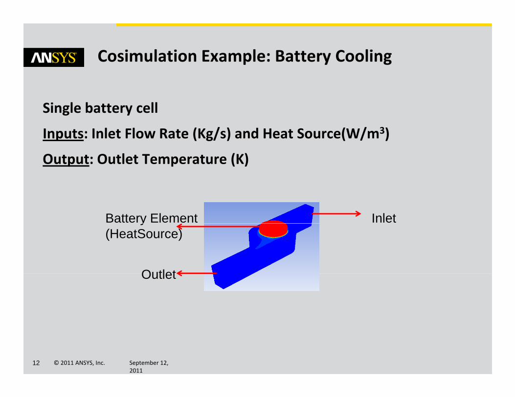
Cosimulation Example: Battery Cooling
Single battery cell
Inputs: Inlet Flow Rate (Kg/s) and Heat Source(W/m3)
Output: Outlet Temperature (K)
InletBattery Element
Outlet
y(HeatSource)
Outlet
© 2011 ANSYS, Inc. September 12, 2011
12

Simulation Results: No Control
Flow Rate
Heat SourceTemperature Change
@250 Sec @1200 Sec
0.01 400k 37.9155 64.8926
800k 75.8207 129.787
0.02 400k 29.7525 39.201
800k 59.4059 78.402
© 2011 ANSYS, Inc. September 12, 2011
13
Results verified with Fluent aloneNon‐linear dependency on Flow Rate
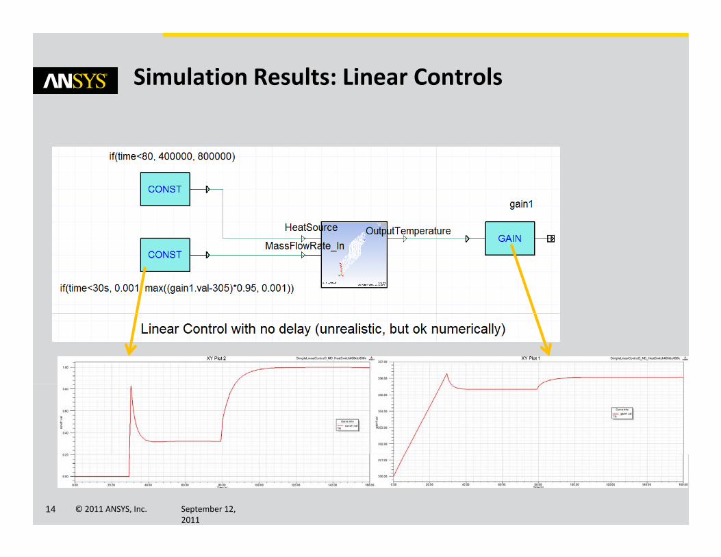
Simulation Results: Linear Controls
© 2011 ANSYS, Inc. September 12, 2011
14
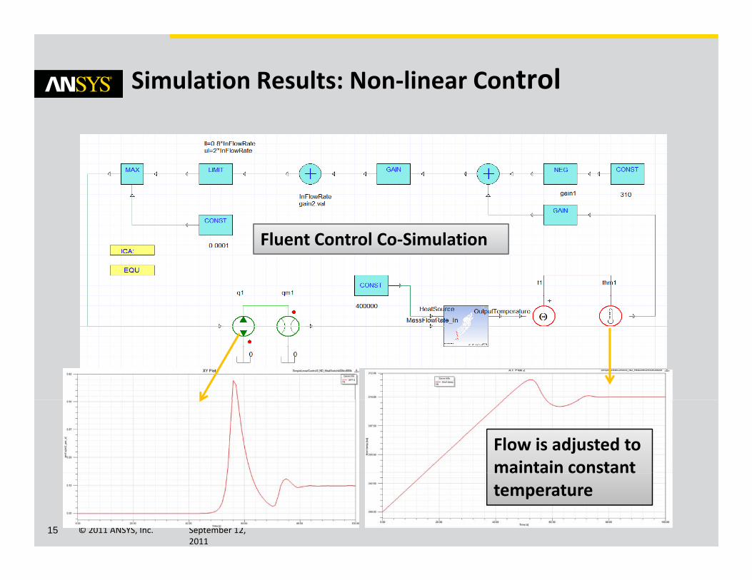
Simulation Results: Non‐linear Control
Fluent Control Co‐Simulation
Flow is adjusted to maintain constant
© 2011 ANSYS, Inc. September 12, 2011
15
maintain constanttemperature
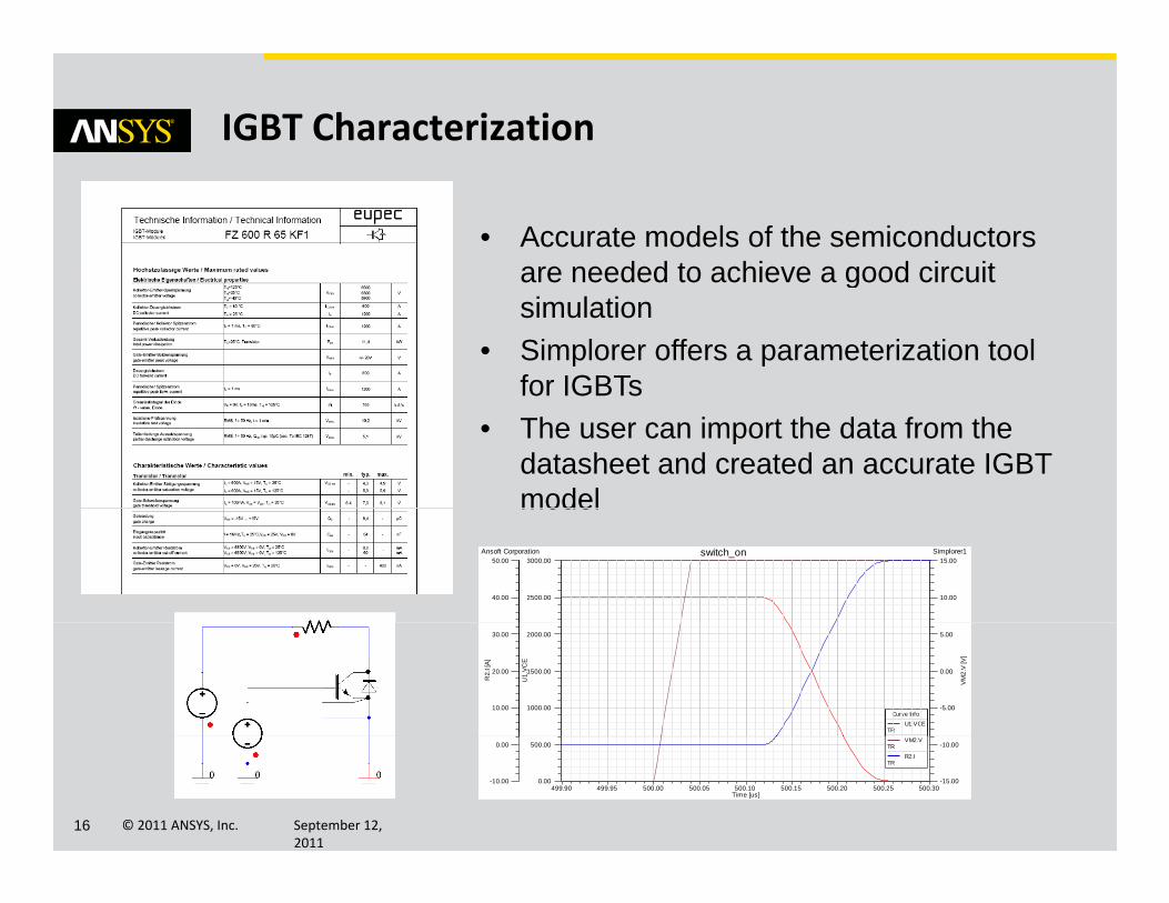
IGBT Characterization
• Accurate models of the semiconductorsare needed to achieve a good circuitare needed to achieve a good circuit simulation
• Simplorer offers a parameterization toolfor IGBTsfor IGBTs
• The user can import the data from the datasheet and created an accurate IGBT modelmodel
2500.00
3000.00
10.00
15.00
40.00
50.00Ansoft Corporation Simplorer1switch_on
2500.00
3000.00
10.00
15.00
40.00
50.00Ansoft Corporation Simplorer1switch_on
1000.00
1500.00
2000.00
U1.
VC
E
-5.00
0.00
5.00
VM
2.V
[V]
10.00
20.00
30.00
R2.
I [A
]
Curve InfoU1.VCE
TR
1000.00
1500.00
2000.00
U1.
VC
E
-5.00
0.00
5.00
VM
2.V
[V]
10.00
20.00
30.00
R2.
I [A
]
Curve InfoU1.VCE
TR
© 2011 ANSYS, Inc. September 12, 2011
16
499.90 499.95 500.00 500.05 500.10 500.15 500.20 500.25 500.30Time [us]
0.00
500.00
-15.00
-10.00
-10.00
0.00VM2.V
TRR2.I
TR
499.90 499.95 500.00 500.05 500.10 500.15 500.20 500.25 500.30Time [us]
0.00
500.00
-15.00
-10.00
-10.00
0.00VM2.V
TRR2.I
TR

IGBT Characterization Improvements
It is possible to customize test circuits in the characterization tool:Every Manufacturer uses different measurement Criteria on their datasheetsEvery Manufacturer uses different measurement Criteria on their datasheets
More optimization and extraction settings have been added
© 2011 ANSYS, Inc. September 12, 2011
17
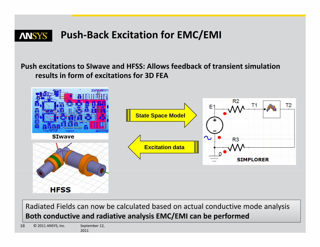
Push‐Back Excitation for EMC/EMI
Push excitations to SIwave and HFSS: Allows feedback of transient simulation results in form of excitations for 3D FEAresults in form of excitations for 3D FEA
State Space Model
Excitation data
© 2011 ANSYS, Inc. September 12, 2011
18
Radiated Fields can now be calculated based on actual conductive mode analysisBoth conductive and radiative analysis EMC/EMI can be performed

SIwave and HFSS Flow
1 Export an equivalent circuit model for the SIwave design as a Simplorer SML netlist
2 Import the SML netlist as a s b circ it2 Import the SML netlist as a sub circuit
• Perform a transient analysis
• Right click to push excitation UI.
3 UI converts time domain signal to frequency domain3 UI converts time domain signal to frequency domain
• Excitation files get writtenExcitation files get written– Voltage and current for each
frequency and port• Import files back to SIwave
l
© 2011 ANSYS, Inc. September 12, 2011
19
– External source excitations

MaxwellMaxwell
2D/3D Finite Element Low Frequency Electromagnetics/ q y g
© 2011 ANSYS, Inc. September 12, 2011
20

Maxwell Overview
• Solves 2D and 3D electromagnetic field problems using FEA
• Five Solution Types: Electrostatic, Magnetostatic, Eddy Current, Transient Electric, Transient Magnetic
• Linear and non-linear, isotropic and anisotropic, and laminated materials
Determines R L C forces torques• Determines R,L,C, forces, torques, losses, saturation, time-induced effects
• Parametric and Optimization capabilities
• Co-simulation with Simplorer
• Direct link from RMxprt
© 2011 ANSYS, Inc. September 12, 2011
21
• Direct link to ANSYS Mechanical
Full Parallelization of 3D non‐transient solvers
Magnetostatic solver:f d– Parameter extractions for inductance
– Energy computation for post processing in field solver
Eddy current solver:– Power loss and stress computation for post processing
– Energy computation for post processing in field solver
© 2011 ANSYS, Inc. September 12, 2011
22
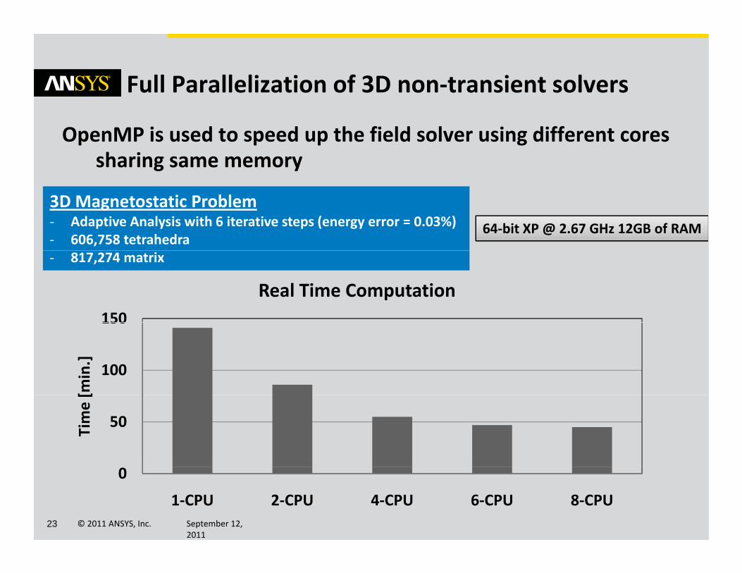
Full Parallelization of 3D non‐transient solvers
OpenMP is used to speed up the field solver using different cores sharing same memory
64‐bit XP @ 2.67 GHz 12GB of RAM
3D Magnetostatic Problem‐ Adaptive Analysis with 6 iterative steps (energy error = 0.03%)‐ 606,758 tetrahedra
150
Real Time Computation
‐ 817,274 matrix
100
150
[min.]
50
Time [
© 2011 ANSYS, Inc. September 12, 2011
23
0
1‐CPU 2‐CPU 4‐CPU 6‐CPU 8‐CPU

3D Eddy Current High Order Elements
Goal: Improve accuracy for current density field (J)
‐ J field is derived quantity from T‐Ω formulationJ field is derived quantity from T Ω formulation
‐ Higher order elements gives first order approximation for currents
© 2011 ANSYS, Inc. September 12, 2011
24
First order approximation for currents
Zero order approximation for currents

3D Eddy Current High Order Elements
C ilCoil
Mesh on the plate
Plate
© 2011 ANSYS, Inc. September 12, 2011
25
Induced eddy current Zero order vector shape functions
Induced eddy currentFirst order vector shape functions
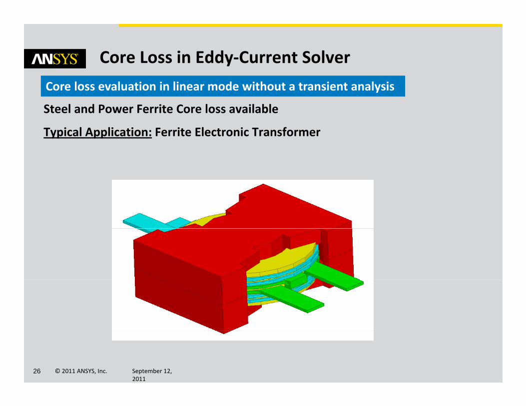
Core Loss in Eddy‐Current Solver
Steel and Power Ferrite Core loss available
Core loss evaluation in linear mode without a transient analysis
Typical Application: Ferrite Electronic Transformer
© 2011 ANSYS, Inc. September 12, 2011
26
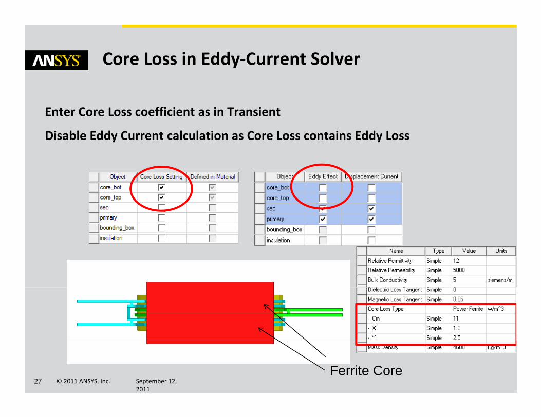
Core Loss in Eddy‐Current Solver
Enter Core Loss coefficient as in Transient
Disable Eddy Current calculation as Core Loss contains Eddy Loss
© 2011 ANSYS, Inc. September 12, 2011
27Ferrite Core

Core loss in Eddy‐Current Solver
Maxwell 3D results: 0.85 W
Formula used:
Validation with hand calculation:
• Core volume = 1.29e‐6 [m^3], frequency= 100KHz
• B ~ 0.2 Tesla
• L 1 29 6 * 11 * (100 000)^1 3 * (0 2)^2 5 0 8 W• Loss = 1.29e‐6 * 11 * (100,000)^1.3 * (0.2)^2.5 = 0.8 W
The core‐loss can be numerically validated using the 3D magnetic transient solver
© 2011 ANSYS, Inc. September 12, 2011
28
The core loss can be numerically validated using the 3D magnetic transient solveremploying linear BH characteristic

Maxwell Integration in Workbench
What was already possible in R13:• Two way thermal coupling with ANSYS Mechanical• Two‐way thermal coupling with ANSYS Mechanical (Static and Transient)
• One‐way force coupling with ANSYS Mechanical (Static and Transient)and Transient)
• One‐way thermal coupling with Fluent through UDF
• Use Design Explorer within WB
idi i l i i• Unidirectional CAD integration
© 2011 ANSYS, Inc. September 12, 2011
29

Maxwell – ANSYS Stress Coupling
Two way coupling non‐transient solvers and ANSYS stress solver is possible in R14is possible in R14
Approach:• The Force distribution is transferred as load into ANSYS MechanicalThe Force distribution is transferred as load into ANSYS Mechanical
• The node displacement information is sent back to Maxwell as deformed mesh
Maxwell ANSYS Mechanical
Force Distribution
Deformed Mesh
© 2011 ANSYS, Inc. September 12, 2011
30

Maxwell – ANSYS Stress Coupling
Example: Air inductor
© 2011 ANSYS, Inc. September 12, 2011
31

Maxwell – ANSYS Stress Coupling
B Field Force Distribution
MagneticForcesForces
Stress CalculationField Calculation
DisplacementsUpdated Mesh
Displacementsof mesh nodes
© 2011 ANSYS, Inc. September 12, 2011
32

Maxwell – Fluent Two‐Way Coupling
Approach:• The Loss distribution is transferred as load into Fluent
• The Temperature distribution is sent back to Maxwell
Maxwell ANSYS Fluent
Loss Distribution
Temperature
© 2011 ANSYS, Inc. September 12, 2011
33
p
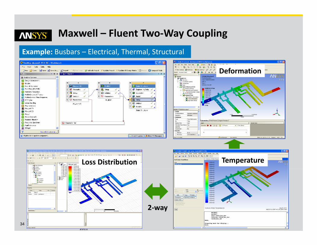
Maxwell – Fluent Two‐Way Coupling
Example: Busbars – Electrical, Thermal, Structural
Deformation
Loss Distribution Temperature
© 2011 ANSYS, Inc. September 12, 2011
34
2‐way

PM Temperature Dependent Model
Maxwell 2D/3D can account for Permanent Magnet temperature dependency. The law works directly on intrinsic BiH curve with
fl d i B d i i i i i Hremanent flux density Br and intrinsic coercivity Hci
HBB i 0The Two temperature dependent parameters are remanent flux
density Br and intrinsic coercivity Hci
B and H can be described by second order polynomials asBr and Hci can be described by second order polynomials as
)()(1)()( 02
02010 TPTBTTTTTBTB rrr
)()( 1)()( 02
02010 TQTHTTTTTHTH cicici
where T0 is the reference temperature, and α1, α2, β1 and β2 are coefficients which are provided in supplier datasheets
)()()()( 002010 Qcicici
© 2011 ANSYS, Inc. September 12, 2011
35

PM Temperature Dependent Model
Copied from vendor datasheet
Derived based on the temperature dependent demagnetization model
© 2011 ANSYS, Inc. September 12, 2011
36
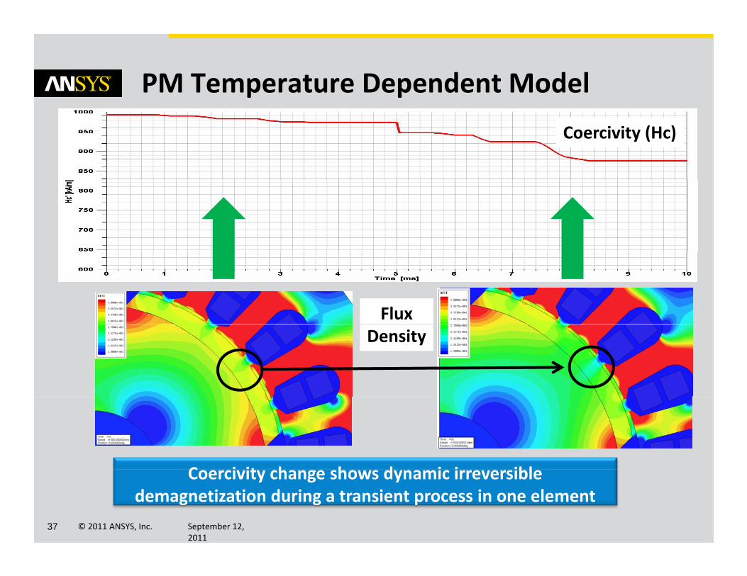
PM Temperature Dependent Model
Coercivity (Hc)
FluxDensity
C i it h h d i i ibl
© 2011 ANSYS, Inc. September 12, 2011
37
Coercivity change shows dynamic irreversible demagnetization during a transient process in one element

Performance Enhancements in 2D Transient Post ProcessingProcessing
• 4096 variations, with 200 time step per variation
• Update and open 2 XY reports• Update and open 2 XY reports
Without Cache With Cache
R13 3 hrs 30 mins 10 mins
R14 32 mins 5 mins 20 secs
Speed up 7X 2X
© 2011 ANSYS, Inc. September 12, 2011
38
Speed up 7X 2X

RMxprt
Analytical Sizing package for Electrical Machine Design
© 2011 ANSYS, Inc. September 12, 2011
39
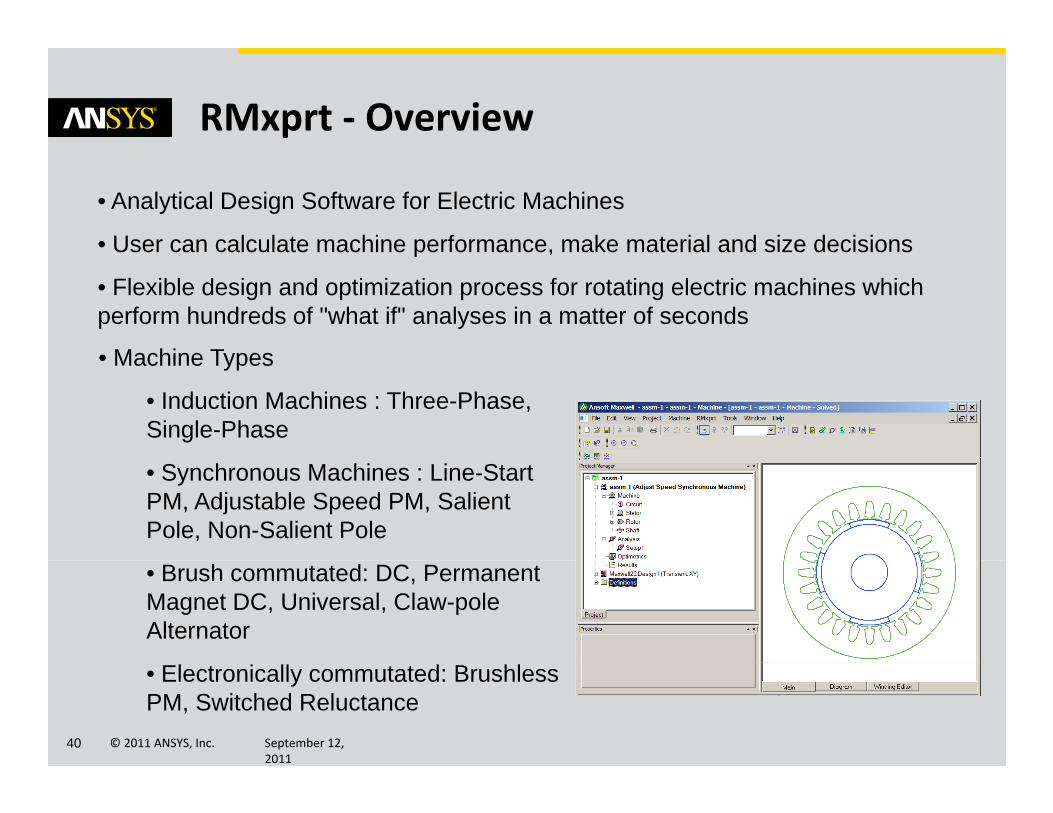
RMxprt ‐ Overview
• Analytical Design Software for Electric Machines
• User can calculate machine performance, make material and size decisionsp ,
• Flexible design and optimization process for rotating electric machines which perform hundreds of "what if" analyses in a matter of seconds
• Machine Types• Machine Types
• Induction Machines : Three-Phase, Single-Phase
• Synchronous Machines : Line-Start PM, Adjustable Speed PM, Salient Pole, Non-Salient Pole
• Brush commutated: DC, Permanent Magnet DC, Universal, Claw-pole Alternator
© 2011 ANSYS, Inc. September 12, 2011
40
• Electronically commutated: Brushless PM, Switched Reluctance

Integrated Motor Solutions
• RMxprt automatic setup with one‐click for Maxwell 2D and 3D Solution• Minimum solving region creation with matching boundary setup • Motion and mechanical setup• Material setup including core loss and lamination• Winding and source setup with drive circuit• Auto‐create Simplorer design
© 2011 ANSYS, Inc. September 12, 2011
41
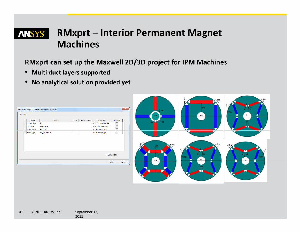
RMxprt – Interior Permanent MagnetMachinesMachines
RMxprt can set up the Maxwell 2D/3D project for IPM Machines• Multi duct layers supported• Multi duct layers supported
• No analytical solution provided yet
© 2011 ANSYS, Inc. September 12, 2011
42
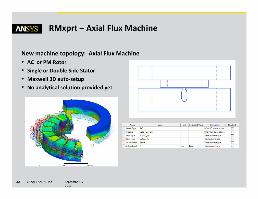
RMxprt – Axial Flux Machine
New machine topology: Axial Flux Machine• AC or PM Rotor• AC or PM Rotor
• Single or Double Side Stator
• Maxwell 3D auto‐setup
• No analytical solution provided yet• No analytical solution provided yet
© 2011 ANSYS, Inc. September 12, 2011
43

Q3D
Quick RLC Extractor for 2D and 3D Structures
© 2011 ANSYS, Inc. September 12, 2011
44

Q3D Extractor ‐ Overview
• Q3D is a tool streamlined for quickly characterizing electrical parasitics (R,L,C,G) of interconnects, busbars and cablesbusbars, and cables.
• Typical Applications:• Switch Mode Power Supplies• Cables, Connectors and Busbar Modeling, g• Ground Plane Modeling• EMI Prediction in Electric Drive Systems
© 2011 ANSYS, Inc. September 12, 2011
45
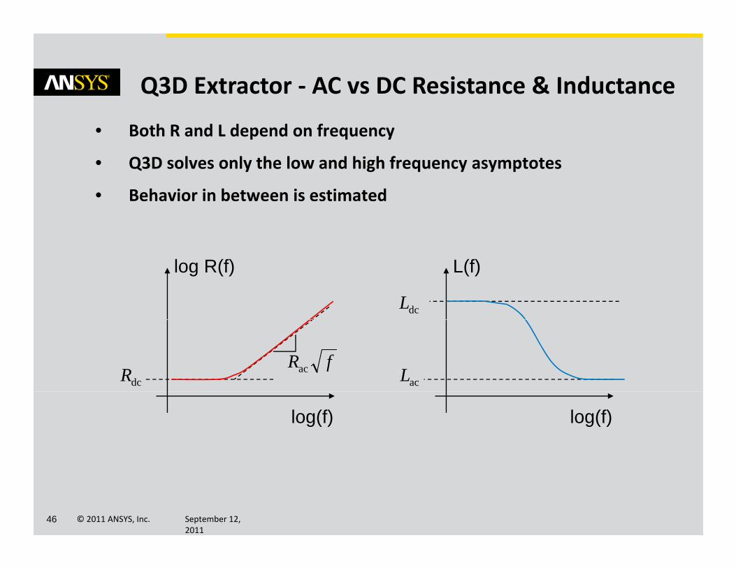
Q3D Extractor ‐ AC vs DC Resistance & Inductance
• Both R and L depend on frequency
• Q3D solves only the low and high frequency asymptotes
• Behavior in between is estimated
log R(f) L(f)
dcL
fRacdcR acL
log(f) log(f)
© 2011 ANSYS, Inc. September 12, 2011
46

Q3D – Magnetic Materials
Q3D can handle Magnetic Materials (in the linear part of B‐H curve)
Permeability can be frequency dependent
Typical Applications:
• Transformers DesignTransformers Design
• Shielding Design
• PCB with Magnetic Core Design
• Q3D uses Boundary elements method to compute RLC parameters• Calculates partial inductance in open
© 2011 ANSYS, Inc. September 12, 2011
47
p ploops

Q3D – Magnetic Materials
Inductor Example
Goal: Get R(f), L(f)
DC < f < 1 MHzDC < f < 1 MHz
Magnetic Core (µ = 500, σ= 100000)
© 2011 ANSYS, Inc. September 12, 2011
48
Solid Copper Coil
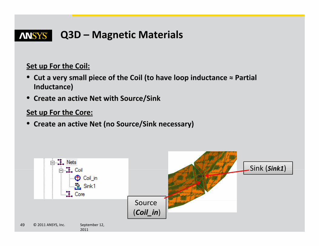
Q3D – Magnetic Materials
Set up For the Coil:
• Cut a very small piece of the Coil (to have loop inductance ≈ Partial• Cut a very small piece of the Coil (to have loop inductance ≈ Partial Inductance)
• Create an active Net with Source/Sink
Set up For the Core:
• Create an active Net (no Source/Sink necessary)
Sink (Sink1)Sink (Sink1)
S
© 2011 ANSYS, Inc. September 12, 2011
49
Source (Coil_in)
Q3D – Magnetic Materials
Using Maxwell:
• FEM Need to mesh to account for skin depth at each frequency• FEM ‐ Need to mesh to account for skin depth at each frequency
• Can lead to huge mesh for higher frequencies as skin depth decreases but gives best accuracy in transition region
T M i l i h f ( f Fi ld f R L)• Two Matrix solutions at each frequency (one for Fields, one for R, L)
Using Q3D:g Q
• BEM – Surface mesh only
• Only 1 resolution for DC, 1 resolution for AC
• Rest of the spectrum determined by blended algorithm• Rest of the spectrum determined by blended algorithm
• No need to mesh for skin depth
• Easier setup but may not give best accuracy in transition region
© 2011 ANSYS, Inc. September 12, 2011
50
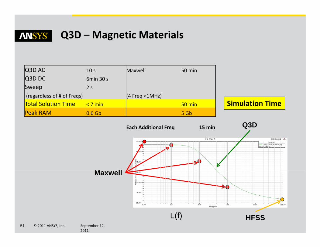
Q3D – Magnetic Materials
Q3D AC 10 s Maxwell 50 min
Q3D DCQ3D DC 6min 30 s
Sweep 2 s
(regardless of # of Freqs) (4 Freq <1MHz)
Total Solution Time < 7 min 50 min Simulation Time
Q3DDesign2XY Plot 1 Q3DDesign2XY Plot 1
Peak RAM 0.6 Gb 5 Gb
Each Additional Freq 15 min Q3D
45.00
50.00
55.00
oil:C
oil_
in) [
nH]
Q3DDesign2XY Plot 1 ANSOFT
Curve InfoACL(Coil:Coil_in,Coil:Coil_in)
Setup1 : Sw eep2
45.00
50.00
55.00
oil:C
oil_
in) [
nH]
Q3DDesign2XY Plot 1 ANSOFT
Curve InfoACL(Coil:Coil_in,Coil:Coil_in)
Setup1 : Sw eep2
M ll
30.00
35.00
40.00
ACL(
Coi
l:Coi
l_in
,Co
30.00
35.00
40.00
ACL(
Coi
l:Coi
l_in
,CoMaxwell
© 2011 ANSYS, Inc. September 12, 2011
51
0.00 0.01 0.10 1.00 10.00 100.00Freq [MHz]
25.00 0.00 0.01 0.10 1.00 10.00 100.00
Freq [MHz]
25.00
L(f) HFSS

Q3D – New Features
Circuit Export:
• Q3D can export frequency dependent models to Simplorer
• Q3D l t R L t ifi f i th d t th• Q3D can also export R, L at a specific frequency in the sweep and export the SPICE netlist or the Simplorer circuit
• The feature has been extended to 2D Extractor
© 2011 ANSYS, Inc. September 12, 2011
52

Q3D ‐ 3D Modeler Enhancements
View customization
• Z-stretch• 64‐bit user interface
© 2011 ANSYS, Inc. September 12, 2011
53
This enhancement is available to all EBU ‐ 3D products

Geometry and User Interface
© 2011 ANSYS, Inc. September 12, 2011
54

Ansoft to ANSYS Geometry Transfer
• Possible import DesignModeler geometry directly into Ansoft products
• Geometry and material assignment transfer from Ansoftsystems to ANSYS systems
• Further geometry edits are possible in DM if user has license
© 2011 ANSYS, Inc. September 12, 2011
55
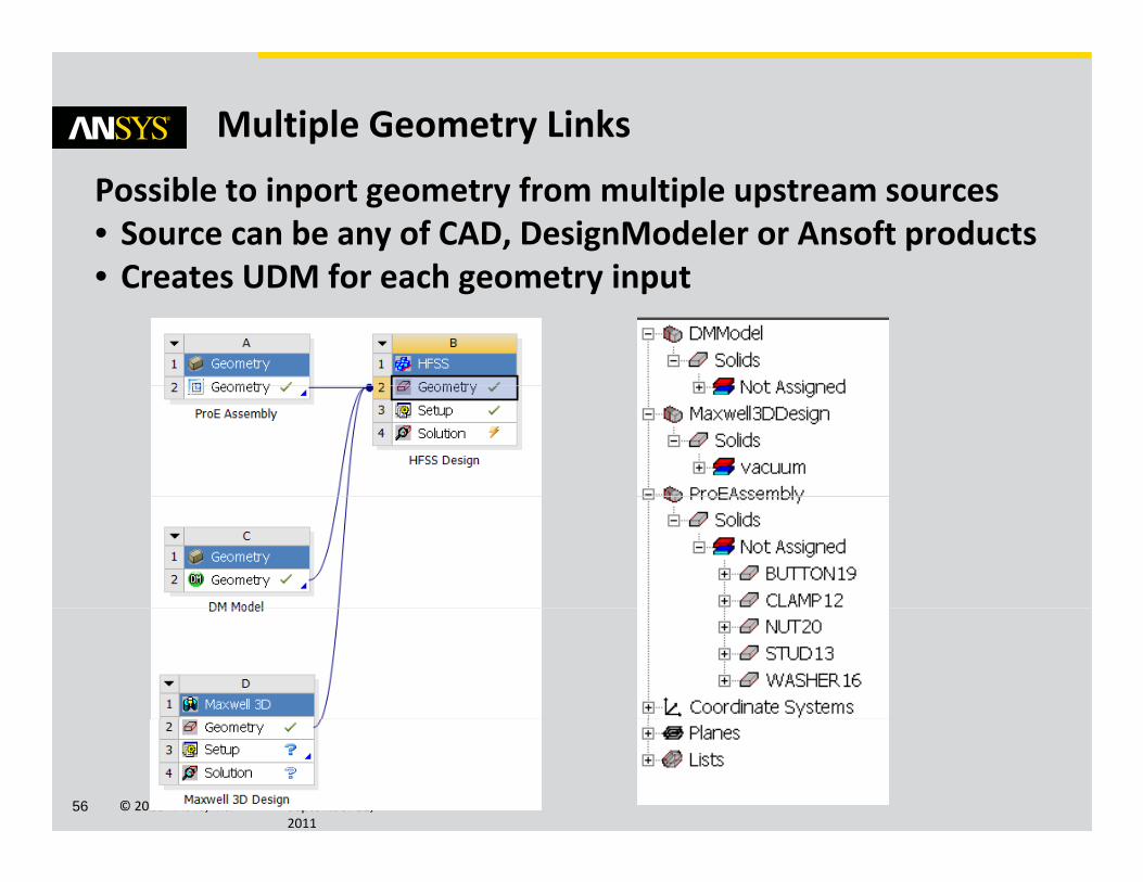
Multiple Geometry Links
Possible to inport geometry from multiple upstream sources• Source can be any of CAD, DesignModeler or Ansoft products• Creates UDM for each geometry input• Creates UDM for each geometry input
© 2011 ANSYS, Inc. September 12, 2011
56
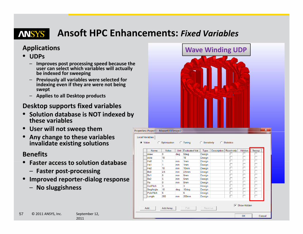
Ansoft HPC Enhancements: Fixed VariablesApplications• UDPs
– Improves post processing speed because the user can select which variables will actually be indexed for sweeping
Wave Winding UDP
be indexed for sweeping– Previously all variables were selected for
indexing even if they are were not being swept
– Applies to all Desktop products
Desktop supports fixed variables• Solution database is NOT indexed by these variables
• User will not sweep themp• Any change to these variables invalidate existing solutions
Benefits• F t t l ti d t b• Faster access to solution database– Faster post‐processing
• Improved reporter‐dialog response– No sluggishness
© 2011 ANSYS, Inc. September 12, 2011
57
gg

CAD Integration on WB Improvements
Added support for parametric analysis and DSO of CAD parameters
© 2011 ANSYS, Inc. September 12, 2011
58

Reliability Engineering Design ‐ DOE
Distribute parametric studies across available hardware to expedite design
i i iIdentify key design parameters
optimization
Identify variation of performance with respect to variations of parameters
© 2011 ANSYS, Inc. September 12, 2011
59

Reliability Engineering Design – Six Sigma
Input parameters vary!A product has Six Sigma quality if only 3.4 parts out of every 1 million manufactured fail
Output parameters
How performance will vary ith d i t l ?
how many parts will likely fail?
which inputs require the greatest control?
© 2011 ANSYS, Inc. September 12, 2011
60
with design tolerances? likely fail? the greatest control?
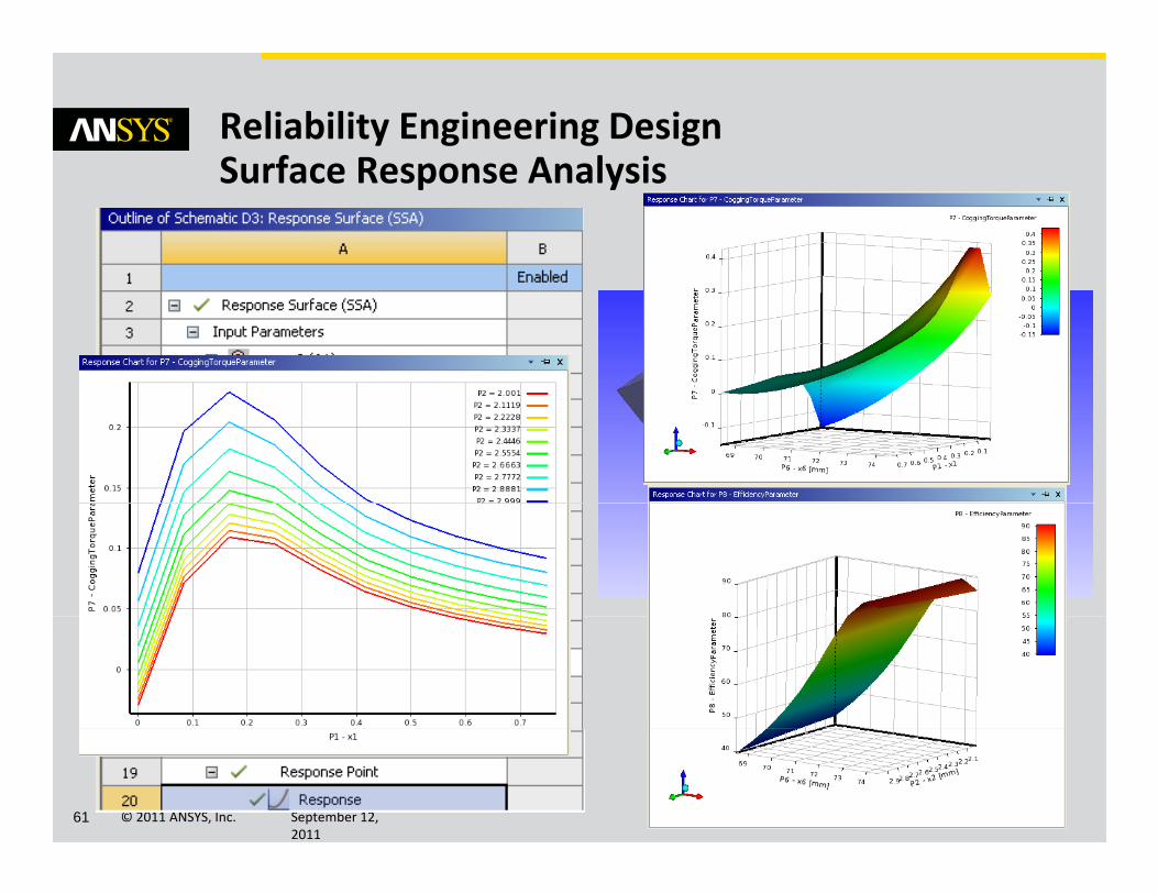
Reliability Engineering DesignSurface Response AnalysisSurface Response Analysis
© 2011 ANSYS, Inc. September 12, 2011
61

Maxwell‐ANSYS Structural and Maxwell ‐ANSYS Thermal Field Mapping coupling capabilities available in R14Field Mapping coupling capabilities available in R14
Maxwell 2D/3D ANSYS Static/Transient StructuralTwo‐Way Link
ANSYS Static/Transient StructuralOne‐Way Link (Maxwell upstream)y y ( p )
Electrostatic
Magnetostatic
ddEddy Current
Magnetic Transient
Electric Transient
Maxwell 2D/3D ANSYS Static/Transient ThermalTwo‐Way Link
ANSYS Static/Transient ThermalOne‐Way Link (Maxwell upstream)
El t t tiElectrostatic
Magnetostatic
Eddy Current
© 2011 ANSYS, Inc. September 12, 2011
62
Magnetic Transient
Electric Transient

Maxwell‐Fluent Field Mapping coupling capabilities available in R14Field Mapping coupling capabilities available in R14
Maxwell 2D/3D Fluent Steady State Fluent TransientMaxwell 2D/3D Fluent Steady State(Thermal link)Two‐Way Link
Fluent Transient(Thermal link)
One‐Way Link (Maxwell upstream)
Electrostatic
Magnetostatic
Eddy Current
M ti T i tMagnetic Transient
Electric Transient
© 2011 ANSYS, Inc. September 12, 2011
63

Simplorer System Coupling capabilities available in R14
Solver Reduce Order Equivalent Co‐Simulation Push BackModel
qCircuit/Matrices/Look‐Up Tables
Excitation
Maxwell 2D/3DElectrostaticMagnetostatic
Maxwell 2D/3Ddd CEddy Current
Maxwell 2D/3DTransient
Q3D
HFSS, SIwave
RMxprt, PExprt
© 2011 ANSYS, Inc. September 12, 2011
64

Simplorer system coupling capabilities available in R14
Solver Reduce Order Equivalent Co‐Simulation Push BackModel
qCircuit/Matrices/Look‐Up Tables
Excitation
Fluent Transient
Icepak
ANSYS Mechanical(Modal)
ANSYS RBD
SimulinkSimulink
ModelSim
Mathcad
© 2011 ANSYS, Inc. September 12, 2011
65
High Frequency Introduction
© 2011 ANSYS, Inc. September 12, 2011
66
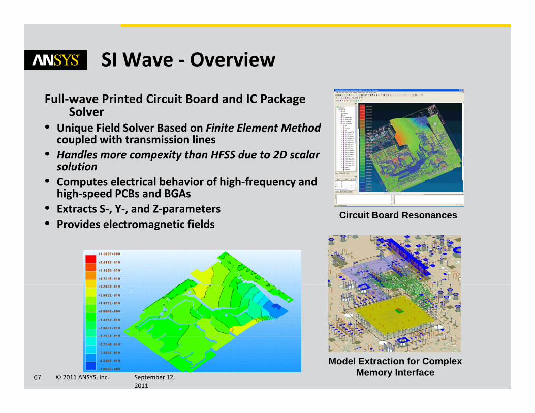
SI Wave ‐ Overview
Full‐wave Printed Circuit Board and IC Package Solver
• Unique Field Solver Based on Finite Element MethodUnique Field Solver Based on Finite Element Methodcoupled with transmission lines
• Handles more compexity than HFSS due to 2D scalar solution
• Computes electrical behavior of high frequency and• Computes electrical behavior of high‐frequency and high‐speed PCBs and BGAs
• Extracts S‐, Y‐, and Z‐parameters• Provides electromagnetic fields
Circuit Board Resonances
© 2011 ANSYS, Inc. September 12, 2011
67
Model Extraction for Complex Memory Interface
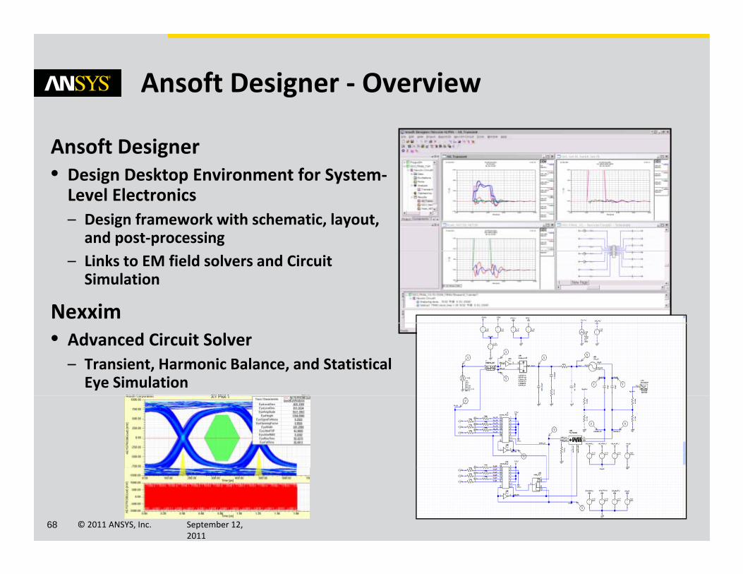
Ansoft Designer ‐ Overview
Ansoft Designer• Design Desktop Environment for System‐Design Desktop Environment for SystemLevel Electronics– Design framework with schematic, layout, and post‐processing
– Links to EM field solvers and Circuit Simulation
Nexxim• Advanced Circuit Solver– Transient, Harmonic Balance, and Statistical Eye Simulation
© 2011 ANSYS, Inc. September 12, 2011
68

HFSS ‐ Overview
Full‐wave 3D electromagnetic field solver• Computes electromagnetic behavior of high‐p g gfrequency and high‐speed components and systems
• Extracts S‐, Y‐, and Z‐parameters• Provides 3D electromagnetic fields• Provides 3D electromagnetic fields
Simulation of RFIC in Package
© 2011 ANSYS, Inc. September 12, 2011
69
Antenna on UAV4-port microwave comparitor
Cavity Filter on cell phone tower
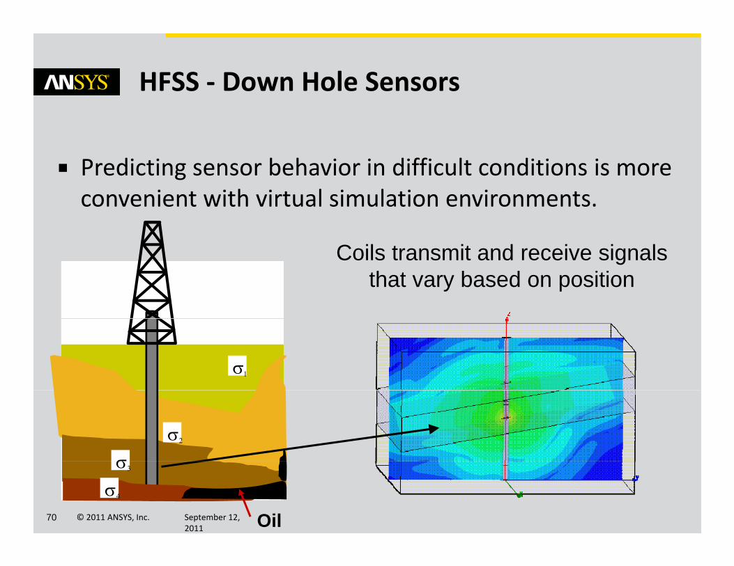
HFSS ‐ Down Hole Sensors
Predicting sensor behavior in difficult conditions is more
C il t it d i i l
gconvenient with virtual simulation environments.
Coils transmit and receive signals that vary based on position
© 2011 ANSYS, Inc. September 12, 2011
70
Oil

HFSS ‐ Down Hole Sensors
Rigorous FEM simulation allows myriad Rigorous FEM simulation allows myriad parametric simulations for the important design variablesvariables
MandrelB h l Borehole
Invasion AnisotropyAnisotropy Eccentricity Antenna Tilt
© 2011 ANSYS, Inc. September 12, 2011
71

HFSS ‐ Down Hole Sensors
Simulation provides accurate calibration data for logs
7.00
8.00Ansoft Corporation HFSSDesign1XY Plot 1
Curve Info
d_mag_importedImported
d_mag
Vary Eccentricity RX Amplitude Ratio
d 0 0005 S/
p g
4.00
5.00
6.00
7.00Y1
Setup1 : LastAdaptiveFreq='0.002GHz'
Dot = LiteratureLine = Ansys
mud = 0.0005 S/m
V Di A l &0.00 1.00 2.00 3.00 4.00 5.00 6.00 7.00
dy [in]2.00
3.00
2.80Ansoft LLC 1_HFSSDesign1XY Plot 4RX Amplitude Ratiomandrel offset Formation = 1 S/m
Dip angle
Vary Dip Angle & Displacement
2.20
2.40
2.60
2.80
litud
e R
atio
Curve Info
Colored = HFSSGreen = Maxwell
formation = 10 S/m Formation = 0.1 S/m
Mud =0.0005 S/m
© 2011 ANSYS, Inc. September 12, 2011
72 -100.00 -80.00 -60.00 -40.00 -20.00 0.00 20.00 40.00 60.00Relative Transmitter Depth [in]
1.60
1.80
2.00
Am
p d_magSetup1 : LastAdaptivedip='0deg' Freq='0.00...
d_magSetup1 : LastAdaptivedip='20deg' Freq='0.0...
d_magSetup1 : LastAdaptivedip='45deg' Freq='0.0...
d_magIncreasing Dip Angle
Formation = 1 S/m
Sondedisplacement