v37-8-1

7/28/2019 v37-8-1

http://slidepdf.com/reader/full/v37-8-1 1/8

Abstract—In this work, new experimental data for slugging

frequency in inclined gas-liquid flow are reported, and a newcorrelation is proposed. Scale experiments were carried out using a

mixture of air and water in a 6 m long pipe. Two different pipediameters were used, namely, 38 and 67 mm. The data were takenwith capacitance type sensors at a data acquisition frequency of 200Hz over an interval of 60 seconds. For the range of flow conditions

studied, the liquid superficial velocity is observed to influence the

frequency strongly. A comparison of the present data withcorrelations available in the literature reveals a lack of agreement. Anew correlation for slug frequency has been proposed for the inclined

flow, which represents the main contribution of this work.

Keywords—slug frequency, inclined flow

I. INTRODUCTION

REVIOUS studies reported in the literature reveal that

intermittent flow exists as the dominant flow pattern in

upward inclined flow. Intermittent flow is characterised bythe variation of the liquid holdup with time, mainly in the

form of periodic structures, such as slugs. The slugging

frequency, f , is in fact defined as the mean number of slugs per unit time as seen by a fixed observer; [11], [7]. To calculate

this parameter, in practice, it is common to recourse to the use

of empirical correlations.

A very much used correlation for slug frequency predictionwas developed by [7] based on data by [11], [17]. Nydal [17]

compared the correlation with experimental data and found a

good fit within the original data range (U SG < 10 m/s and U SL

< 1.3 m/s).

⎥

⎦

⎤⎢

⎣

⎡⎟

⎠

⎞⎜

⎝

⎛ + U m

U m

gd

U .= f

SL

S

75.1902260

2.1

(1)

V. Hernandez-Perez, the corresponding author, is a research fellow in the

Process and Environmental Engineering Research Division, Chemical and

Environmental Engineering Department, University of Nottingham. Emailaddress: [email protected]

M. Abdulkadir is a PhD student in the Process and Environmental

Engineering Research Division, Chemical and Environmental Engineering

Department, University of Nottingham.

B. J. Azzopardi is Lady Trent Professor and Head of the Department of Chemical and Environmental Engineering, University of Nottingham.

A correlation was suggested by [8]. This model is on the

same form as the [7] correlation,

( )⎥⎦

⎤⎢

⎣

⎡+

gd

U

d U

U .= f m

m

SL

S

2

2.1

02.202260 (2)

Heywood and Richardson [10] proposed the following

correlation, being almost identical to the one from [7], but based on a much larger amount of experimental data,

⎥⎦⎤

⎢⎣⎡

⎟⎟ ⎠

⎞⎜⎜⎝

⎛ +

gd

U

d .= f m

LS

2

02.1

02.204340 λ (3)

Tronconi [18] presented a semi-mechanistic expression for the slug frequency, where the slug frequency was assumed to

be half the frequency of unstable waves (slug precursors),

h

U Cw.= f

g

G

L

GS

ρ

ρ 13050 −(4)

Where U G=U SG/(1- H L) and hG is the height of the gas phaseat the inlet, immediately upstream the point of slug initiation.

C w is the wave velocity of the waves growing to become slugs.

Tranconi [18] postulated a linear relationship between the

frequency of critical waves and the slug frequency, f w= C w f S ,with C w=2. This corresponds to observations in slug flow (by

[4] and [13], where every second slug originating from these

waves was unstable and disappeared. The [18] correlation

does not directly take into consideration any change in slugfrequency with changing liquid flow rate, but indirectly

through the calculations of gas flow rate and height.

Nydal [17] argued that, at high liquid flow rates, the slugfrequency should depend weakly on U SG, but strongly on U SL,

and suggested a correlation based on the liquid flow rate

alone,

( ) gd

U .= f

SL

S

5.10880

2

+(5)

Jepson and Taylor [12] published data from the 306 mm

pipe diameter rig of the Harwell laboratory, and the effect of

diameter was investigated by including 25.4 and 51.2 mm pipe

Slugging Frequency Correlation for Inclined

Gas-liquid Flow

V. Hernandez-Perez*, M. Abdulkadir, B. J. Azzopardi

P

World Academy of Science, Engineering and Technology 37 2010

44

7/28/2019 v37-8-1


data from [16]. A non-dimensional slug frequency wascorrelated against the superficial mixture velocity,

).+U *( d

U = f m

SLS

0101059.7 3−(6)

Manolis et al. [15] developed a new correlation based on

[7]. Taking U m,min=5 m/s and the modified Froude number

⎥⎦

⎤⎢⎣

⎡ +

U

U U

gd

U = Fr

m

mmSL22

min,mod (7)

Where

Fr .= f S

8.1

mod00370 (8)

Zabaras [21] suggested a modification to the [7] correlation,

where the influence of pipe inclination angle was included,

equation (9). The data on which the modified correlation was

tuned included positive pipe angles in the range of 0 to 11°

relative to the horizontal.

( )θ sin2.75+0.836

75.1902260

2.1

•+ ⎥⎦

⎤⎢⎣

⎡⎟

⎠

⎞⎜⎝

⎛ U m

U m gd

U .= f

SL

S

(9)

All the above correlations are for horizontal flow. As aresult, it is expected that when applied to other inclinations,

they will fail to predict the frequency. In an effort to provide a

tool for frequency calculation in inclined flow, a new

correlation is reported in the present work, based onexperimental data.

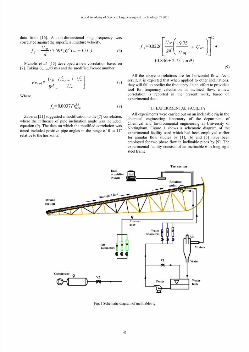
II. EXPERIMENTAL FACILITY

All experiments were carried out on an inclinable rig in the

chemical engineering laboratory of the department of

Chemical and Environmental engineering at University of Nottingham. Figure 1 shows a schematic diagram of the

experimental facility used which had been employed earlier

for annular flow studies by [1], [6] and [5] have beenemployed for two phase flow in inclinable pipes by [9]. The

experimental facility consists of an inclinable 6 m long rigid

steel frame.

Airrotameters

Test section

Mixing

section

V2

Data

acquisitonsystem

SISTEMADE

ADQUISICION

DE DATOS

G a s - l i q u i d f l o

w

Waterrotameters

Watertank

Water

Pump

Mixture

Air

Compressor

Pressuregage

V1

Rotation

point

Fig. 1 Schematic diagram of inclinable rig


45

7/28/2019 v37-8-1


The test pipe is mounted on this frame and could be rotated between vertical to horizontal in 5○ increments meaning the

effect of different inclinations could be monitored. Two pipe

diameters were studied, namely 38 mm and 67mm. Thistesting section is made up of shorter pipes. Each shorter pipe

can be easily installed or replaced.Air from the laboratory 6 bara compressed air main was

used as the gas phase. It is fed into the facility through a 0.022

m internal diameter stainless steel pipe. A pressure regulating

valve sets the maximum air inlet pressure and a pressure relief

valve, set at 100% of the required feed pressure protects thefacility against overpressure. Both the airflow rate and gage

pressure are measured prior to entering the mixing section

using a set of rotameters that covered a wide range of flow

rates as well a pressure gage meter respectively. Inlet

volumetric flow rates of water are determined prior to enteringthe mixing section with a set of rotameters that cover the range

from 0-0.73 m/s of superficial velocities. The two separate

phases are then mixed at the gas liquid mixing section. Fromthe mixing section, the two-phase mixture flows along the

inclined pipe before reaching the test section where thecapacitance sensors are located. The pipe outlet is connected

to the separator tank open to the atmosphere.

In the separator air is released to the atmosphere from thetop of the separator and liquid is settled under the influence of

gravity and flows through the bottom to return to main liquid

tank.This rig used an air-water mixture to examine the behaviour

of gas-liquid flows in an inclined pipe. The sensor was placed

at about 5.15 m away from the mixing section. The

experiments were performed at room temperatures (15-20degree Celsius)

III. RESULTS AND DISCUSSION

In order to determine the frequency of periodic structures(slugs) the methodology of Power Spectral Density (PSD) was

applied. In addition the number of slugs visible on the liquid

holdup time traces was counted. The latter was carried out

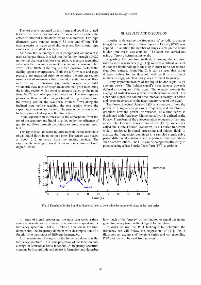
using different discrimination levels.Regarding the counting method, following the criterion

used by most researchers (e.g. [17]) we used a critical value of

0.7 for the liquid holdup in the slug in order to be consideredslug flow pattern. From Fig. 2, it can be seen that using

different values for the threshold will result in a different

number of slugs, which in turn gives a different frequency.

A very important feature of the liquid holdup signal is itsaverage power. The holdup signal’s instantaneous power is

defined as the square of the signal. The average power is the

average of instantaneous powers over their time interval. For a periodic signal, the natural time interval is clearly its period

and the average power is the mean square value of the signal.The Power Spectral Density, PSD, is a measure of how the

power in a signal changes over frequency and therefore, itdescribes how the power (or variance) of a time series is

distributed with frequency. Mathematically, it is defined as the

Fourier Transform of the autocorrelation sequence of the time

series. The Discrete Fourier Transform (DFT), sometimescalled the Finite Fourier Transform, is a Fourier transform

widely employed in signal processing and related fields to

analyze the frequencies contained in a sampled signal, solve partial differential equations, and to perform other operations

such as convolutions. The DFT can be computed efficiently in

practice using a Fast Fourier Transform (FFT) algorithm.

0 2 4 6 8 10 12 14 16 18 200

0.2

0.4

0.6

0.8

1

Time (s)

L i q u i d

H o l d u p

Threshold

Slugs Waves

Fig. 2 Threshold for the liquid holdup level used to determine the number of slugs in the time series

In terms of signal processing, the transform takes a timeseries representation of a signal function and maps it into a

frequency spectrum. That is, it takes a function in the time

domain into the frequency domain; with decomposition of a

function into harmonics of different frequencies.A representation of a signal in the frequency domain is the

frequency spectrum. This is the projection of the function onto

a range of sinusoidal basis functions. A frequency spectrum

contains both amplitude and phase information and describes

how much of the "energy" of the function or signal lies in anygiven frequency band, without regard for the phase.

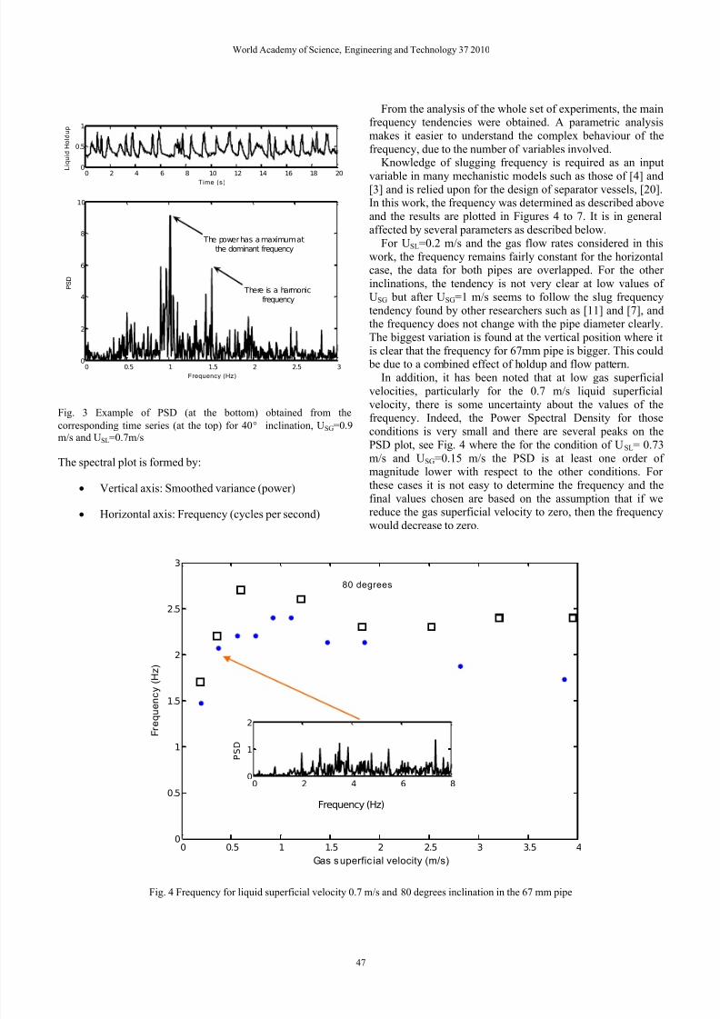
In order to use the PSD technique to determine the

frequency we will follow the suggestions of [11]. Fig. 3

illustrates an example of the time series and correspondingPSD plot that will be used from now on.


46

7/28/2019 v37-8-1


0 2 4 6 8 10 12 14 16 18 200

0.5

1

Time (s)

L i q u i d

H o l d u p

0 0.5 1 1.5 2 2.5 30

2

4

6

8

10

Frequency (Hz)

P S D

The power has a maximum at

the dominant frequency

There is a harmonic

frequency

Fig. 3 Example of PSD (at the bottom) obtained from the

corresponding time series (at the top) for 40° inclination, USG=0.9m/s and USL=0.7m/s

The spectral plot is formed by:

• Vertical axis: Smoothed variance (power)

• Horizontal axis: Frequency (cycles per second)

From the analysis of the whole set of experiments, the mainfrequency tendencies were obtained. A parametric analysis

makes it easier to understand the complex behaviour of the

frequency, due to the number of variables involved.Knowledge of slugging frequency is required as an input

variable in many mechanistic models such as those of [4] and[3] and is relied upon for the design of separator vessels, [20].In this work, the frequency was determined as described above

and the results are plotted in Figures 4 to 7. It is in general

affected by several parameters as described below.

For USL=0.2 m/s and the gas flow rates considered in this

work, the frequency remains fairly constant for the horizontalcase, the data for both pipes are overlapped. For the other

inclinations, the tendency is not very clear at low values of

USG but after USG=1 m/s seems to follow the slug frequency

tendency found by other researchers such as [11] and [7], andthe frequency does not change with the pipe diameter clearly.

The biggest variation is found at the vertical position where it

is clear that the frequency for 67mm pipe is bigger. This could be due to a combined effect of holdup and flow pattern.

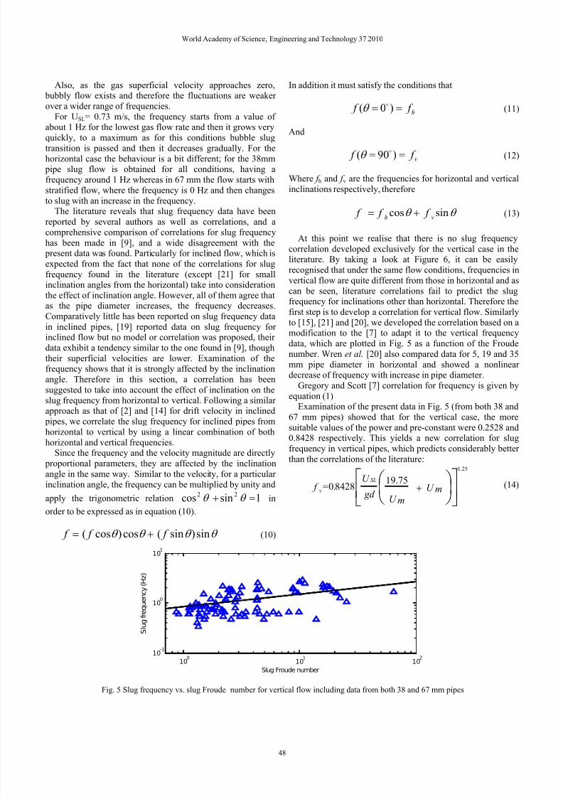
In addition, it has been noted that at low gas superficial

velocities, particularly for the 0.7 m/s liquid superficial

velocity, there is some uncertainty about the values of thefrequency. Indeed, the Power Spectral Density for those

conditions is very small and there are several peaks on the

PSD plot, see Fig. 4 where the for the condition of USL= 0.73

m/s and USG=0.15 m/s the PSD is at least one order of magnitude lower with respect to the other conditions. For

these cases it is not easy to determine the frequency and the

final values chosen are based on the assumption that if wereduce the gas superficial velocity to zero, then the frequency

would decrease to zero.

0 0.5 1 1.5 2 2.5 3 3.5 40

0.5

1

1.5

2

2.5

3

Gas superfic ial velocity (m/s)

F r e q u

e n c y

( H z )

80 degrees

Fig. 4 Frequency for liquid superficial velocity 0.7 m/s and 80 degrees inclination in the 67 mm pipe

0 2 4 6 80

1

2

Frequency (Hz)

P S D


47

7/28/2019 v37-8-1


Also, as the gas superficial velocity approaches zero, bubbly flow exists and therefore the fluctuations are weaker

over a wider range of frequencies.

For USL= 0.73 m/s, the frequency starts from a value of about 1 Hz for the lowest gas flow rate and then it grows very

quickly, to a maximum as for this conditions bubble slugtransition is passed and then it decreases gradually. For the

horizontal case the behaviour is a bit different; for the 38mm pipe slug flow is obtained for all conditions, having a

frequency around 1 Hz whereas in 67 mm the flow starts with

stratified flow, where the frequency is 0 Hz and then changes

to slug with an increase in the frequency.The literature reveals that slug frequency data have been

reported by several authors as well as correlations, and a

comprehensive comparison of correlations for slug frequency

has been made in [9], and a wide disagreement with the present data was found. Particularly for inclined flow, which is

expected from the fact that none of the correlations for slug

frequency found in the literature (except [21] for smallinclination angles from the horizontal) take into consideration

the effect of inclination angle. However, all of them agree thatas the pipe diameter increases, the frequency decreases.

Comparatively little has been reported on slug frequency data

in inclined pipes, [19] reported data on slug frequency for inclined flow but no model or correlation was proposed, their

data exhibit a tendency similar to the one found in [9], though

their superficial velocities are lower. Examination of thefrequency shows that it is strongly affected by the inclination

angle. Therefore in this section, a correlation has been

suggested to take into account the effect of inclination on the

slug frequency from horizontal to vertical. Following a similar approach as that of [2] and [14] for drift velocity in inclined

pipes, we correlate the slug frequency for inclined pipes fromhorizontal to vertical by using a linear combination of both

horizontal and vertical frequencies.Since the frequency and the velocity magnitude are directly

proportional parameters, they are affected by the inclination

angle in the same way. Similar to the velocity, for a particular

inclination angle, the frequency can be multiplied by unity and

apply the trigonometric relation 1sincos 22 =+ θ θ in

order to be expressed as in equation (10).

θ θ θ θ sin)sin(cos)cos( f f f += (10)

In addition it must satisfy the conditions that

h f f == )0( Dθ (11)

And

v f f == )90(D

θ (12)

Where f h and f v are the frequencies for horizontal and vertical

inclinations respectively, therefore

θ θ sincos f f f vh

+= (13)

At this point we realise that there is no slug frequency

correlation developed exclusively for the vertical case in theliterature. By taking a look at Figure 6, it can be easily

recognised that under the same flow conditions, frequencies in

vertical flow are quite different from those in horizontal and ascan be seen, literature correlations fail to predict the slugfrequency for inclinations other than horizontal. Therefore the

first step is to develop a correlation for vertical flow. Similarly

to [15], [21] and [20], we developed the correlation based on amodification to the [7] to adapt it to the vertical frequency

data, which are plotted in Fig. 5 as a function of the Froude

number. Wren et al. [20] also compared data for 5, 19 and 35

mm pipe diameter in horizontal and showed a nonlinear decrease of frequency with increase in pipe diameter.

Gregory and Scott [7] correlation for frequency is given by

equation (1)Examination of the present data in Fig. 5 (from both 38 and

67 mm pipes) showed that for the vertical case, the moresuitable values of the power and pre-constant were 0.2528 and0.8428 respectively. This yields a new correlation for slug

frequency in vertical pipes, which predicts considerably better

than the correlations of the literature:

⎥⎦

⎤⎢⎣

⎡⎟ ⎠

⎞⎜⎝

⎛ + U m

U m gd

U .= f

SL

v

75.1984280

25.0

(14)

100

101

102

10-1

100

101

Slug Froude number

S l u g f r e q u e n c y ( H z )

Fig. 5 Slug frequency vs. slug Froude number for vertical flow including data from both 38 and 67 mm pipes


48

7/28/2019 v37-8-1


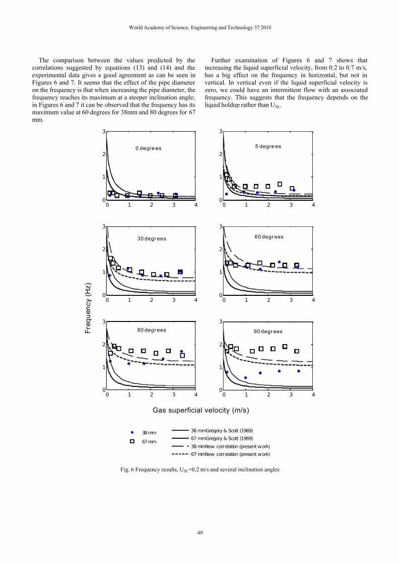
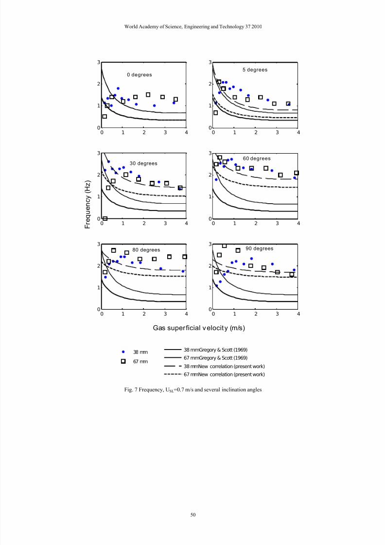
The comparison between the values predicted by thecorrelations suggested by equations (13) and (14) and the

experimental data gives a good agreement as can be seen in

Figures 6 and 7. It seems that the effect of the pipe diameter on the frequency is that when increasing the pipe diameter, the

frequency reaches its maximum at a steeper inclination angle;in Figures 6 and 7 it can be observed that the frequency has itsmaximum value at 60 degrees for 38mm and 80 degrees for 67

mm.

Further examination of Figures 6 and 7 shows thatincreasing the liquid superficial velocity, from 0.2 to 0.7 m/s,

has a big effect on the frequency in horizontal, but not in

vertical. In vertical even if the liquid superficial velocity iszero, we could have an intermittent flow with an associated

frequency. This suggests that the frequency depends on theliquid holdup rather than USL.

0 1 2 3 40

1

2

3

0 degre es

0 1 2 3 40

1

2

3

5 degre es

0 1 2 3 40

1

2

3

30 degr ees

0 1 2 3 40

1

2

3

60 degr ees

0 1 2 3 4

0

1

2

3

Gas superficial velocity (m/s)

F r e q u e n c y ( H z )

80 degr ees

0 1 2 3 4

0

1

2

3

90 degr ees

38 mm

67 mm

38 mmGregory & Scott (1969)


38 mmNew correlation (present work)


Fig. 6 Frequency results, USL=0.2 m/s and several inclination angles


49

7/28/2019 v37-8-1


0 1 2 3 40

1

2

3

0 degrees

0 1 2 3 40

1

2

3

5 degrees

0 1 2 3 40

1

2

3

30 degrees

0 1 2 3 40

1

2

360 degrees

0 1 2 3 40

1

2

3

Gas superficial velocity (m/s)

F r e q u e n c y ( H

z )

80 degrees

0 1 2 3 40

1

2

390 degrees

38 mm

67 mm





Fig. 7 Frequency, USL=0.7 m/s and several inclination angles


50

7/28/2019 v37-8-1


IV. CONCLUSION

New experimental data for slugging frequency in inclined

gas-liquid flow are reported and the following conclusions can be drawn:

When analysing the frequency, it was found that it is a verycomplex parameter and therefore care must be taken when

performing the calculations. Also interpretation of the result isimportant to verify the values, since the frequency is a very

fundamental parameter of intermittent flow and it is used

together with the translational velocity for the calculation of slug length.

A comparison of the present data with correlations available

in the literature reveals a lack of agreement. A new correlation

for slug frequency has been proposed for the inclined flow,which represents the main contribution of this work.

NOMENCLATURE

Symbol Description, Units

d Diameter of the tube, mm

Cw Unstable waves

f Frequency, Hz

g Gravity constant, 9.81 m/s2

U m Mixture homogeneous velocity, m/s

U S Slug velocity, m/s

U SG Gas superficial velocity, m/s

U SL Liquid superficial velocity, m/s

Greek Symbols

θ Inclination angle with respect to horizontal, °

λ U SL /U m

Subscripts

h Horizontal

L Liquid

m Mixture

min Minimum

s Slug

Dimensionless numbers Fr Froud Number, Fr m=U m

2/ gd

R EFERENCES

[1] Azzopardi, B.J., 1997, Drops in annular two-phase flow, International

Journal of Multiphase Flow, Vol. 23, pp. 1-53.

[2] Bendiksen, K. H., (1984), “An experimental investigation of the motionof long bubbles in inclined tubes”, International Journal of Multiphase

Flow, Vol. 10, No. 4, pp. 467-483.

[3] Cook, M. and Behnia, M., (2000), “Pressure drop calculation andmodelling of inclined intermittent gas-liquid flow”, ChemicalEngineering Science, Vol. 55, No. 20, pp. 4699-4708.

[4] Dukler, A. E. and Hubbard, M. G., (1975), “A Model for Gas-LiquidSlug Flow in Horizontal and Near Horizontal Tubes”, Ind. Eng. Chem.

Fundamentals, Vol. 14, No. 4, pp. 337-347.

[5] Geraci, G., Azzopardi, B. J., and Van Maanen, H. R. E., ( 2007b),

“Effect of inclination on circumferential film thickness variation inannular gas/liquid flow”, Chemical Engineering Science, Vol. 62, No.

11, pp. 3032-3042.

[6] Geraci, G., Azzopardi, B. J., and Van Maanen, H. R. E., ( 2007a),

“Inclination effects on circumferential film flow distribution in annular

gas/liquid flows”, AIChE Journal, Vol. 53, No. 5, pp. 1144-1150.[7] Gregory, G. A. and Scott, D. S., (1969), “Correlation of liquid slug

velocity and frequency in horizontal co-current gas-liquid slug flow”,

AIChE Journal , Vol. 15, pp. 833-835.

[8] Greskovich, E. J. and Shrier, A. L., (1972), “Slug frequency inhorizontal gas-liquid slug flow”, Ind. Eng. Chem. Proc. Design Dev.,

Vol. 11, No. 2, pp. 317-318.

[9] Hernandez-Perez, V., 2007, Gas-liquid two-phase flow in inclined pipes,

a PhD Thesis, University of Nottingham, United Kingdom.[10] Heywood, N. I. and Richardson, J. F., (1979), “Slug Flow of Air-Water

Mixtures in a Horizontal Pipe: Determination of Liquid Hold-up by -rayAbsorption”, Chemical Engineering Science, Vol. 34, pp. 17-30.

[11] Hubbard, M. G., (1965), “An analysis of horizontal gas-liquid slug”, Ph.

D. Thesis, University of Houston, Houston USA .

[12] Jepson, W. P. and Taylor, R. E., (1993), “Slug flow and its transitions inlarge-diameter horizontal pipes”, International Journal of Multiphase

Flow, Vol. 19, No. 3, pp. 411-420.

[13] Kordyban, E. S., (1985), “Some Details of Developing Slugs in

Horizontal Two-Phase Flow”, AIChE J., Vol. 31, pp. 802.

[14] Malnes, D., (1983), “Slug flow in vertical, horizontal and inclined pipes”, Tech. Rep. IFE/KR/E-83/002 Rev. 1987, Institute for Energy

Technology.[15] Manolis, I G., Mendes-Tatsis M A., and Hewitt, G F., (1995), “The

effect of pressure on slug frequency on two-phase horizontal flow”, The2nd conference on multiphase flow, Kyoto, Japan, April 3-7, 1995.

[16] Nicholson, M. K., Aziz, K., and Gregory, G. A., (1978), “Intermittent

two-phase flow in horizontal pipes: Predictive models”, The Canadian

Journal of chemical engineering, Vol. 56, pp. 653-663.

[17] Nydal, O. J., (1991), “An experimental investigation of slug flow”, PhD

thesis, University of Oslo.[18] Tronconi, E., (1990), “Prediction of Slug Frequency in Horizontal Two-

Phase Slug Flow”, AIChE Journal, Vol. 36, No. 5, pp. 701-709.

[19] Van Hout, R., Shemer, L., and Barnea, D., (2003), “Evolution of

hydrodynamic and statistical parameters of gas-liquid slug flow alonginclined pipes”, Chemical Engineering Science, Vol. 58, No. 1, pp. 115-

133.

[20] Wren, E., Baker, G., Azzopardi, B. J., and Jones, R., (2005), “ Slug flowin small diameter pipes and T-junctions ”, Experimental Thermal and

Fluid Science, Vol. 29, No. 8, pp. 893-899 .[21] Zabaras, G. J., (1999), “Prediction of slug frequency for gas-liquid

flows”, Annual Technical Conference, SPE 56462, pp. 181-188.


51

Documents

v37-8-1