Vacillation cycles and blocking in a channel

Q. J. R. Meteorol. SOC. (19981,124, pp. 873-895

Vacillation cycles and blocking in a channel By K. €NINES* and A. J. HOLLAND

University of Edinburgh, UK

(Received 16 December 1996; revised 5 August 1997)

SUMMARY The response to a low-level high-frequency wavemaker forcing in a two-layer, 8-plane, quasi-geostrophic

channel model is examined. The wavemaker simulates regular baroclinic instability which then propagates to upper atmospheric levels to excite blocking. By altering the meridional shear in the upper layer, the large-scale response can vary from a steady large-amplitude split jet, very similar to observed blocks, to a weaker split with a low-frequency vacillation cycle. The eddies will always resonantly excite the split flow, but a mixed instability process is responsible for the breakdown in cases which oscillate, and this is demonstrated using a simplified zonal stability analysis and energy-tendency diagnostics. The re-excitement by the eddies continues the cycle. This model provides a theory of how the meridional structure of the upper-level winds may determine whether a large-amplitude block can be excited or persist in the presence of similar high-frequency eddy activity propagating up from below.

KEYWORDS: Blocking Eddy/mean-flow interaction Low-frequency variability

1. INTRODUCTION

Atmospheric blocking has been studied intensively for the last decade because of its important influence on weather and regional climate, and the difficulty of predicting blocking events or reproducing them within General Circulation Models (GCMs). An important influence on blocking studies was the proposal by Green (1977), that high-frequency transient eddies within the atmospheric storm tracks might play a role in maintaining the anomalous vorticity budget during blocking events. Numerous diagnostic studies using data e.g. Illari (1984), Shutts (1986), Hoskins et al. (1985), Dole (1986, 1989), and GCMs e.g. Mullen (1986), Branstator (1992), appear to confirm the importance of interactions between the smaller-scale, high-frequency, eddies and larger-scale blocking waves. Un- fortunately none of these studies gives direct indication that improved predictability may be possible, because transient cyclones are generated continuously in the storm tracks and the vast majority of them do not go on to initiate blocking. Studies by Dole (1986, 1989), Mo and Ghil(1988), Vautard (1990) and Plaut and Vautard (1994) found consistent large scale blocking-precursor flow patterns, and Vautard et al. (1996) attempted to use these precursors to investigate predictive skill. However this work remains mostly descriptive unless some theoretical foundations can be found. To have a chance of understanding any necessary precursors for blocking, a simpler modelling approach is needed.

Perhaps the most convincing, and the simplest, model of eddies exciting a block can be found in Shutts (1983), where an equivalent barotropic channel is used with a wavemaker to artificially produce high-frequency eddies. This model produced a continuous state of blocking downstream of the region of eddy generation, which Shutts showed to be due to eddy vorticity fluxes. The scale of the excited block is the stationary Rossby wave scale within the channel. Shutts also showed that blocking does not occur for more rapid flows in which a stationary wave cannot be excited. This suggests that an accessible quasi-steady free-mode state may be a necessary pre-condition for blocking, The atmosphere may always have blocking-like free states available if one considers the modon or soliton waves, e.g. McWilliams (1980), Haines and Marshall (1987), Haines and Malanotte-Rizzoli (1991), Flier1 and Haines (1994), which can persist in a wide variety of zonal flows. However modons were not found in the Shutts (1983) study and we need to

* Corresponding author: Department of Meteorology, University of Edinburgh, JCMB, Kings Buildings, Mayfield Road, Edinburgh EH9 352, UK. e-mail: [email protected].

873

874 K. HAINES and A. J. HOLLAND

understand more clearly what factors control the resonant response of a jet stream to the presence of transient eddies in order to make further progress.

Vautard and Legras (1988) extended the Shutts model to two layers and dispensed with the wavemaker, maintaining instead a short region of baroclinity using thermal forcing. They showed convincingly that sometimes blocking did occur downstream, when a large- amplitude stationary wave develops, and sometimes the downstream flow is more zonal. This result, while more realistic than the continuous blocking of Shutts, does not explore other influences on the frequency or persistence of blocking. In particular, variations in the mean flow which may be influenced by larger-scale events, e.g. teleconnections and variations in planetary-wave amplitudes, such as the Pacific/North American pattern and the North Atlantic Oscillation, might have an influence on blocking frequency and hence make blocking more predictable. Recent results in two areas suggest that this may be so.

Thorncroft et al. (1993) showed that changes in horizontal shear can influence the late- stage nonlinear life cycles of baroclinic waves. They hinted that different life cycles may then have different probabilities of exciting a block. Secondly, Ferranti et al. (1994) have shown that tropical sea surface temperatures (SSTs) may influence blocking frequency in middle latitudes, presumably by modifying transient-cyclone behaviour although this is not demonstrated. For a more detailed review see Haines (1994). These results have inspired us to return to simple models of blocking, forced by eddies, to try to address mean-flow influences on blocking.

Section 2 describes the basic model framework consisting of a two-layer quasi- geostrophic channel, like that of Vautard and Legras (1988), but with a wavemaker to produce eddies within the lower layer. The forcing/dissipation balances in the two layers are discussed. Section 3 presents results for a vertically sheared flow without horizontal shear. Section 4 describes the changes upon introducing a meridional shear to the jet stream in the upper layer. Section 5 presents a stability and energy analysis for the growth and decay of the observed jet-splitting events. Section 6 provides discussion and conclusions.

2. THEMODEL

A two-layer, zonally periodic, B-plane, quasi-geostrophic channel is used, satisfying the following equation:

for i = 1,2, where

q is the quasi-geostrophic potential vorticity, @ is the stream function with subscript 1 for the lower layer and 2 for the upper layer. The Jacobian may be rewritten as J(@, q ) = v.Vq = V.(vq). W is a wavemaker forcing, is the Kronecker function, and @/ is a spec- ified initial zonal flow towards which relaxation occurs. E and K are dissipation parameters and S(x) is a sponge layer. The planetary-vorticity gradient /? = 1.6 x lo-" m-ls-l, and the deformation-radius parameter y 2 = 7.844 x m-2. The width of the channel is 6000 km and the length is 20 000 km with a resolution dx = dy = 200 km.

VACILLATION CYCLES AND BLOCKING 875

(a) The wavemaker In the atmosphere transient eddies grow strongly by conversion of low-level avail-

able potential energy. The wave activity produced then propagates to upper levels where meridional air-parcel displacements may become very large due to the decrease in air density, and the waves become nonlinear. Eliassen-Palm fluxes, e.g. Edmon et al. (1980), can be used to follow the vertical and rneridional propagation of the wave activity in a zonal-mean framework. The physical distinction between the region of wave generation (near the surface) and the region of nonlinear wave breaking and blocking initiation (at upper levels) suggests that a wavemaker could reasonably be substituted as an eddy source at low levels.

The use of a wavemaker is not a retrograde step from the work of Vautard and Legras (1988). Its use recognizes that baroclinic growth is a low-level phenomenon and is therefore, to some extent, independent of the initiation of any blocking at upper levels during the mature stage of storm life cycles, as in Thorncroft et al. (1993). With a wavemaker at lower levels, the wave activity at upper levels increases due to vertical propagation from below in a mostly conservative fashion, as it would with a truly unstable low-level source. This aspect cannot be captured in a barotropic model in which the wavemaker and jet stream are in the same layer. The upward-propagation phase still provides an opportunity for feedback where the presence of the block affects the transient-eddy behaviour. Diabatic processes must also play a part in cyclone development. At low levels the availability of surface moisture from a warm ocean helps to fix the baroclinic zones, again independently of the upper-level jet-stream structure. Although diabatic processes also affect upper levels they mostly play a dissipative role, so that wave growth and breaking is essentially a function of the low-level source and the upward-propagation path of the eddies. The wavemaker framework simplifies the possible feedbacks considerably, allowing more freedom in choosing the upper-layer flow conditions which in turn feedback on high-frequency wave propagation.

In this model the wavemaker, W, is placed in the lower layer with the form:

W ( X , y , t ) = E(x, y ) cos (kx - ot) xo < x < xg + L, (4)

where L, = 4360 km, L , = 2730 km and k = 2n/(2900 km). This wavemaker is based on that of Shutts (1983) and gives zero forcing in a spatial- or temporal-average sense. The period of the wavemaker corresponds to 4.5 days, i.e. a 2.25-day time-scale for each synoptic system. Although the upper-layer flow is altered immediately by introduction of vorticity into the lower layer, the upper-layer potential vorticity is not directly modified, and so irreversible changes in upper-layer time-mean flow can only occur through wave breaking and dissipation. However, local reversible changes may still occur whose nature becomes clear if the flow returns to its previous configuration downstream of the region of eddy activity, Plumb (1990).

(b) The dissipation Values of the dissipation parameters are E = 1.92 x s-l and K = 4 x lo5 m2s-l.

The Laplacian dissipation term V2(@ - @ I ) has a vorticity dissipation coefficient S ( x ) which increases E by a factor of 1000 in the last fifth of the channel; this provides a sponge to prevent the re-circulation of the wavemaker eddies. All dissipation terms relax


the upper-layer flow back to a zonal flow +i(y), which may include a meridional wind shear. The lower-layer flow is kept small by the vorticity dissipation because @: = 0 in all of the runs reported here. This choice is made because the mean surface winds are much weaker than those at upper atmospheric levels. This also means that the vorticity introduced by the wavemaker in the lower layer is not immediately advected downstream.

(c ) Stationary Rossby waves and stability criterion To interpret the results it is useful to first review the stationary-wave properties of the

zonal flows used. If the zonal flow in the channel is defined by:

@: = O ,

where U is the constant upper-layer wind; then if U > 14.6 m s-l no antisymmetric stationary waves can exist in the channel. If U = 7.3 m s-l an antisymmetric stationary wave has the same zonal length-scale as the channel width, i.e. 6000 km. In any case stationary waves are confined to the upper layer where they remain solutions at any amplitude; in the lower layer they are always with zero amplitude. This is true provided U < B / y 2 = 20.4 m s-l, otherwise the zonal flow becomes baroclinically unstable with aq:/ay negative. For any more general upper-layer flow with nonlinear +;(y), the lin- ear stationary wavelength changes with latitude, and exact solutions cannot be found at finite amplitude. All of the zonal flows studied here will be initially stable, although the most interesting cases are those close enough to the stability limit for the presence of a superimposed block to make the flow locally supercritical. Two factors might support the study of such jets: first, Stone (1972) suggested that the baroclinic waves are efficient at maintaining the atmospheric jet close to the critical-stability limit, at least in a zonally averaged sense; second, most intense baroclinic activity occurs near the surface while the middle and upper troposphere, considered in isolation, may be less unstable.

( d ) Eddylmean-flow interaction In order to understand the dominant features of the eddy/mean-flow interaction we

can consider the unforcedlundamped momentum equations at upper levels. By separating the flow into time-mean and eddy components (e.g. @ = @M + @’), the mean zonal and meridional momentum equations may be written:

auM a(uM)2 a(uMuM) a(d2)M a(U’d)M -+- + at ax a Y

+- + - ByuM - fo~g = 0, (6) ax a Y

a u M a(uM)2 U M ) a(d2)M a ( d d ) M -+- + ByUM + f ” U t = 0. (7) ax +- +

a t a Y + ax ay

The subscript ‘ag’ denotes ageostrophic components; velocity terms without sub- scripts are geostrophic. The largest eddy terms in the model arise in the region over the wavemaker, which is defined to produce eddies which are meridionally elongated, consistent with the findings of Hoskins et al. (1983) for high-pass eddies. This means that


( u ’ ~ ) ~ S ( d 2 j M or ( u ’ u ’ ) ~ and the dominant eddy term is a(u’2)M/ay in (7), as discussed in Hoskins (1983).

The mean vorticity, CM, equation can then be written as:

(8) a 2 ( d d ) M

ax2 = O .

a y U ’ 2 - U’2jM aZ(U’VI)M

ayax a Y + - +

The a ( ~ ’ ~ ) ~ / d y term_ becomes a2(v’2)M/axay in the vorticity equation. Because of the amplitude envelope W over the wavemaker, ( u ’ ~ ) ~ will be a maximum at the centre of the region. The double derivative acting on this dominant term in (8) then gives rise to a quadrupole component in the eddy forcing e.g. Fig. 2(b). If only the last eddy term in (8) can be neglected then the Hoskins (1983) E-vector can be derived. Otherwise, when written out in full, the eddy feedback is J($‘, (’)M = V . ( V ’ < ’ ) ~ , which forms a component of the potential-vorticity eddy feedback.

3. UNIFORM UPPER-LAYER FLOW

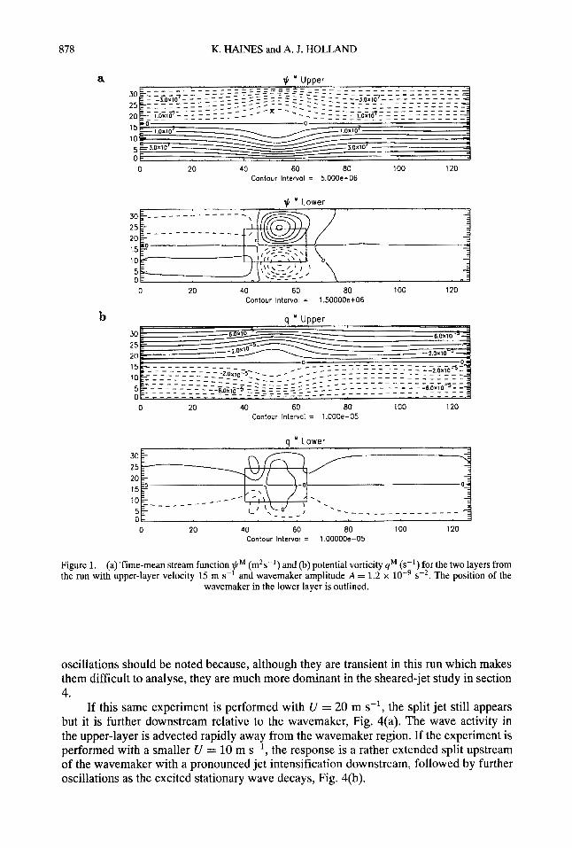
For uniform upper-layer flow @:(yj = - U y . The wavemaker was switched on with amplitude A = 1.2 x lop9 sp2 and the model was integrated for 360 days with the final 200 days being used for diagnostics. We show first results with U = 15 m s-’, close to the limit for stationary-wave activity. Although this flow is baroclinically stable, the potential- vorticity gradient in the lower layer is considerably reduced, so that the presence of any large-scale waves may affect the flow stability. Figure 1 shows the upper- and lower-layer means, @ M and qM, over the 200-day period. A large-amplitude dipole block develops which is equivalent barotropic, with strong easterly flow in the lower layer and almost no flow in the upper layer between the dipole vortices. The wavemaker position is outlined in Fig. 1 by a rectangle. The split jet stream in the upper-layer is close to a free state with $M

and qM contours nearly parallel, however a neutral stationary Rossby wave would have no flow in the lower layer. The strong low-layer circulation is therefore directly spun-up by the wavemaker. There is little sign of stationary-wave activity downstream of the block, and the mean flow returns to its zonal state without oscillations.

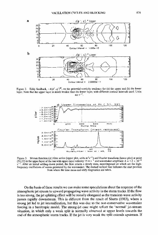
If the balance of terms in the mean upper-layer potential-vorticity budget is analysed, the main balance is between mean flow advection and dissipation in the region of the block. The transient-eddy forcing term is an order of magnitude smaller, however when it is displayed in Fig. 2(a) the characteristic bowed structure can be seen, as eddies are deformed in the split jet-entrance region.

It is the forcing by eddies in the lower layer and the consequent existence of the large lower-layer dipole which is vital to maintaining the upper-layer split. The small size of the eddy forcing at upper levels has always been a problem in studying eddy forcing from atmospheric diagnostics, as pointed out by Shutts (1986). To test the nature of the excitation of the mean response we took the eddy-feedback terms from both layers, as shown in Fig. 2, and used them as steady forcing terms instead of the wavemaker. The steady response in both layers was indistinguishable from that shown in Fig. 1. Figure 3 shows a time series of $2 at the position marked with a cross in the upper model layer on Fig. l(a) for the wavemaker run. After the initial build-up period, the time series of .\ct shows a few low-frequency oscillations before settling down with weak, regular, high-frequency eddies passing through the block and little sign of any other frequencies. The initial low-frequency


a

b

0 20 40 60 80 100 120 Contour Interval = 5.000et06


0 20 40 60 80 100 120 Contour Interval = 1.000e-05


Figure 1. the run with upper-layer velocity 15 m s-l and wavemaker amplitude A = 1.2 x

(a) Time-mean stream function $M (m2s-') and (b) potential vorticity qM (s-I) for the two layers from s - ~ . The position of the

wavemaker in the lower layer is outlined.

oscillations should be noted because, although they are transient in this run which makes them difficult to analyse, they are much more dominant in the sheared-jet study in section 4.

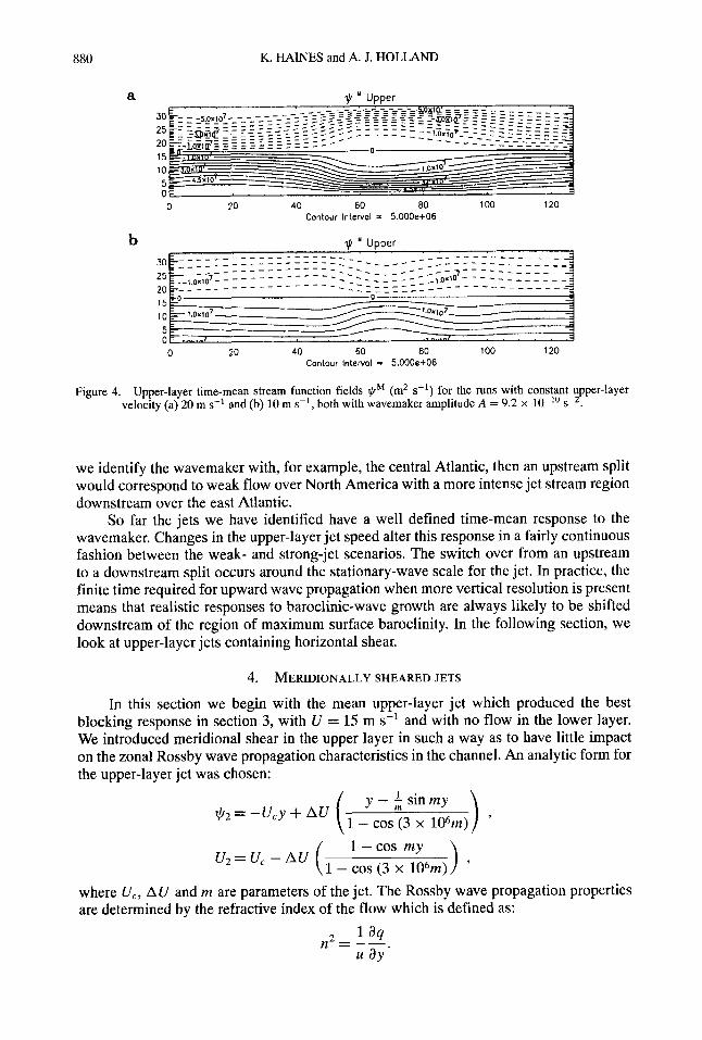
If this same experiment is performed with U = 20 m s-', the split jet still appears but it is further downstream relative to the wavemaker, Fig. 4(a). The wave activity in the upper-layer is advected rapidly away from the wavemaker region. If the experiment is performed with a smaller U = 10 m s-l, the response is a rather extended split upstream of the wavemaker with a pronounced jet intensification downstream, followed by further oscillations as the excited stationary wave decays, Fig. 4(b).


a 30 25 20 15 10

5 0

Contour lntervol = 1.000e- 12

b 30 25 20 15 10 5 0

0 20 40 60 BO 100 120 Contour lntervol = 2.00000e-11

Figure 2. Eddy feedback, -J($', q')', on the potential-vorticity tendency for (a) the upper and (b) the lower layer. Note that the upper layer is much weaker than the lower layer, with different contour intervals used. Units

are s - ~ .

b - 6 . 0 ~ 1 0 ~

- 1 . 4 x 107

0 200 400 600 800 Dump Step

Fourier Transform (mean removed) ' . " " " '

/ - L..-/Jv> 5 . 0 ~ 1 0 ~

Figure 3. Stream function ($) time series (upper plot, units m2s-') and Fourier transform (lower plot) at point (51,22) in the upper layer of the run with upper-layer velocity 15 m s-l and wavemaker amplitude A = 1.2 x s - ~ . After an initial settling-down period, the flow retains a steady state, superimposed on which are the high- frequency oscillations of waves generated by the wavemaker. The dashed vertical line indicates the start position

from where the time mean and eddy diagnostics are taken.

On the basis of these results we can make some speculations about the response of the atmospheric jet stream to upward propagating wave activity in the storm tracks. If the flow is too strong, the jet splitting effect will be zonally elongated as the transient-wave activity passes rapidly downstream. This is different from the result of Shutts (1983), where a strong jet led to jet intensification, but this was due to the non-conservative wavemaker forcing in a barotropic model. The strong-jet case might reflect the 'normal' jet-stream situation, in which only a weak split is normally observed at upper levels towards the end of the atmospheric storm tracks. If the jet is very weak the split extends upstream. If


0 20 40 60 80 100 120 Contour lntervol = 5.000et06

- - - - - _ _ _ - _ b


Figure 4. Upper-layer time-mean stream function fields $rM (m2 s-l) for the runs with constant upper-layer velocity (a) 20 m s-' and (b) 10 m s-', both with wavemaker amplitude A = 9.2 x lo-'' s-*.

we identify the wavemaker with, for example, the central Atlantic, then an upstream split would correspond to weak flow over North America with a more intense jet stream region downstream over the east Atlantic.

So far the jets we have identified have a well defined time-mean response to the wavemaker. Changes in the upper-layer jet speed alter this response in a fairly continuous fashion between the weak- and strong-jet scenarios. The switch over from an upstream to a downstream split occurs around the stationary-wave scale for the jet. In practice, the finite time required for upward wave propagation when more vertical resolution is present means that realistic responses to baroclinic-wave growth are always likely to be shifted downstream of the region of maximum surface baroclinity. In the following section, we look at upper-layer jets containing horizontal shear.

4. MERIDIONALLY SHEARED JETS

In this section we begin with the mean upper-layer jet which produced the best blocking response in section 3, with U = 15 m s-' and with no flow in the lower layer. We introduced meridional shear in the upper layer in such a way as to have little impact on the zonal Rossby wave propagation characteristics in the channel. An analytic form for the upper-layer jet was chosen:

1 y - sin my 1 - cos (3 x 106m)

+z = -U,y 4- AU

where U,, AU and m are parameters of the jet. The Rossby wave propagation properties are determined by the refractive index of the flow which is defined as:


a b C

- E v

W

C a m 0

1

0 5 10 15 20 Speed u (ms-' )

Upper Layer

h

E v

0

c 0 c

a

3000

- 1000

-3000

Upper Layer

Figure 5. (a) Upper layer velocity u (m s-I); (b) upper layer potential-vorticity gradient dq/dy (m-'s-' x lo-"), the vertical thin line represents planetary-vorticity values, with the upper layer to the right and the lower layer to the left; (c) upper layer refractive index n2 (m-2 x In each case results are given for two jets. Jet 1 (bold full line) is the constant 15 m s-', jet 2 (dashed line) is the case with horizontal shear. See text for further explanation.

We chose the parameters such that n2 in the centre of the upper layer remained the same as for the uniform jet stream with U = 15 m SKI. For the main experiment we used U, = 19 m s-l, AU = 18 m s-l, m = 5.2 x m-l, with meridional profiles shown in Fig. 5. The jet shear has the effect of bringing the initial flow even closer to the critical limit for stability. In this case the presence of a blocking wave will be shown to have a more profound influence on the stability of the jet than was seen in section 3.

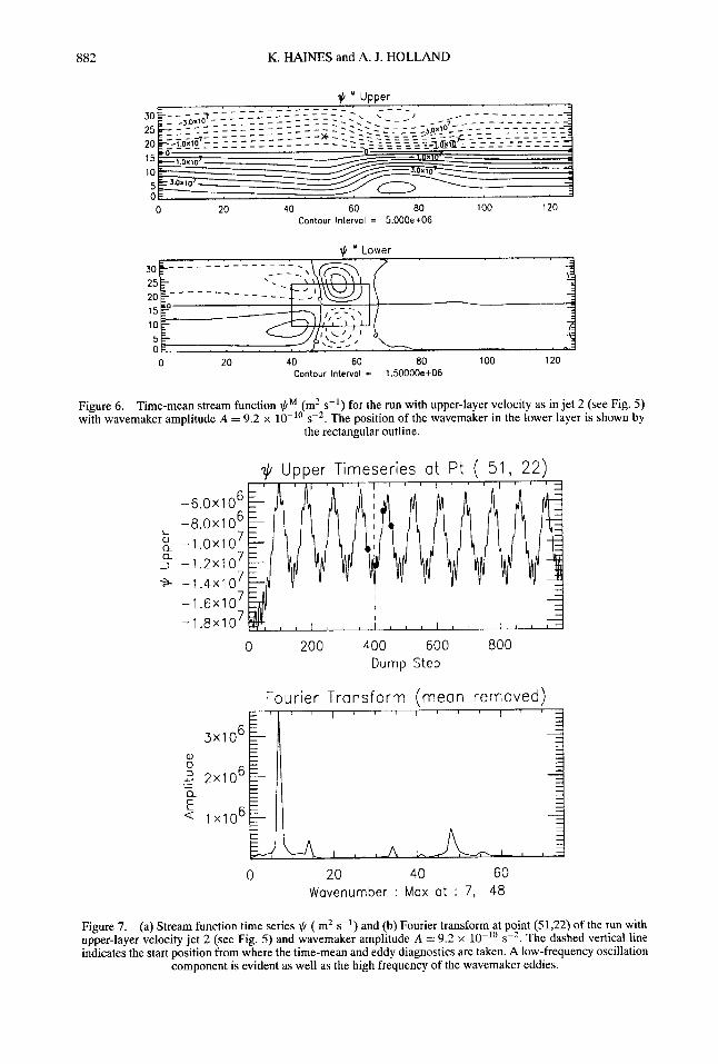
With a reduced wavemaker amplitude (A = 9.2 x lo-'' sP2) the model was run for 400 days with the final 300 days used for diagnostics. Figure 6 shows the time-mean stream function QM in each layer. The position of the upper-layer split is similar to that in Fig. 1. The mean flow splits over the wavemaker although with some stationary-wave activity downstream, similar to the weak-jet response in Fig. 4(b).

Figure 7 shows the time series and Fourier transform of + in the upper layer at the position marked in Fig. 6(a). Clearly a radical change has taken place. As well as the high- frequency eddy activity which can still be seen, the flow now exhibits a low-frequency oscillation between higher amplitude split-jet states (which we will refer to as blocked although they are weaker than in Fig. 1) and more zonal flow states. From Fig. 7 it can be seen that the low-frequency oscillation is quite regular with a period of 31 days. Note that the high- and low-frequency oscillations are not phase locked, as can be seen, for example, from the distribution of high-frequency eddy signatures around the peaks of the low-frequency oscillation.

As the low-frequency oscillation is very regular, we performed a Fourier analysis on the stream-function field which allows a separation of the instantaneous flow as follows:

+ = llrM + + L + llrH 9

where pbL and +H are the low- and high-frequency eddy components respectively. The low- frequency component of the flow can be studied at different phases of the oscillation cycle. Figure 8(a-h) shows $M+L and qM+L in both layers for the four phases: zonal, growth, blocked and decaying; these phases are marked in that order on Fig. 8. Figure 8(i-1) shows the feedback of the high-frequency eddies onto the mean and low-frequency flow at the different oscillation phases. These figures contain clues about the processes responsible for the low-frequency oscillation, and we will consider them in more detail.



0 20 40 60 80 100 120 Contour Interval = 1.50000e+06

Figure 6 . Time-mean stream function $rM (m2 s-') for the run with upper-layer velocity as in jet 2 (see Fig. 5 ) with wavemaker amplitude A = 9.2 x lo-'" s-'. The position of the wavemaker in the lower layer is shown by

the rectangular outline.

$ Upper Timeseries a t P t ( 51, 22) 6 -6.OX10 6 -8.OX10 7

Q 7 3 -1.2x10

7 3 -1.4X10 7 -1.6X10 7

L : -1.ox10

-1.8x10

0 200 400 600 800 Dump Step

Fourier Transform (mean removed) I J ' ' 1 " ' ~ ' '

3x106 W TI 6 .- 2 2x10

Q 1x106

- a E

L.

0 20 40 60 48 Wavenumber : Max at : 7 ,

Figure 7. (a) Stream function time series $r ( m2 s - ' ) and (b) Fourier transform at point (51,22) of the run with upper-layer velocity jet 2 (see Fig. 5) and wavemaker amplitude A = 9.2 x lo-'" s-*. The dashed vertical line indicates the start position from where the time-mean and eddy diagnostics are taken. A low-frequency oscillation

component is evident as well as the high frequency of the wavemaker eddies.


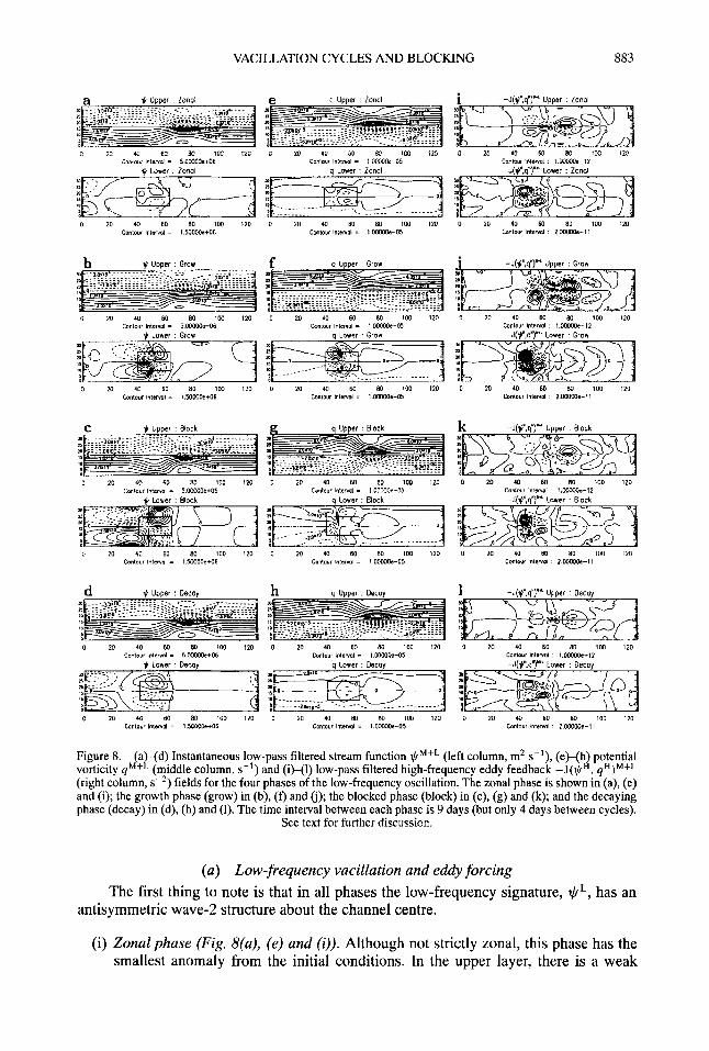
Figure 8. (a d) Instantaneous low-pass filtered stream function $M+L (left column, m2 SKI), ( e H h potential vorticity q'+qmiddle column, s-l) and (iH1) low-pass filtered high-frequency eddy feedback -J($d, qH)M+L (right column, s - ~ ) fields for the four phases of the low-frequency oscillation. The zonal phase is shown in (a), (e) and (i); the growth phase (grow) in (b), (f) and 6); the blocked phase (block) in (c), (g) and (k); and the decaying phase (decay) in (d), (h) and (1). The time interval between each phase is 9 days (but only 4 days between cycles).

See text for further discussion.

(a) Low-frequency vacillation and eddy forcing The first thing to note is that in all phases the low-frequency signature, @L, has an

antisymmetric wave-2 structure about the channel centre.

(i) Zonal phase (Fig. 8(u), (e) and (i)). Although not strictly zonal, this phase has the smallest anomaly from the initial conditions. In the upper layer, there is a weak


widening of the contours over the wavemaker region, with an intensification further downstream. The lower layer shows only a very weak anomaly forming over the wavemaker region. The high-frequency eddy forcing is developing in the upper layer with an anticyclonic-over-cyclonic dipole above the wavemaker. In the lower layer the quadrupole is weaker than in Fig. 2(b).

(ii) Growth phase (Fig. 8(b), (' and 0)). In this phase, 9 days later, there is an obvious difference in the lower layer, where a quadrupole in both circulation and potential vorticity has developed. In the upper layer, upstream of the wavemaker, the flow is more zonal but a split is developing over the wavemaker. At this phase the high- frequency eddy forcing is very strong in both upper and lower layers.

(iii) Blocked phase (Fig. 8(c), (g) and (k)). The upper-layer flow is now at its most split over the wavemaker region, with the downstream intensification also strong. The lower-layer circulation anomaly has extended a little upstream and the lower potential-vorticity quadrupole has weakened and separated meridionally. The high- frequency eddy forcing has weakened considerably in both layers compared with the growth phase.

(iv) Decayphase (Fig. 8(d), (h) and ( I ) ) . The upper-layer split now extends well upstream of the wavemaker. In the lower layer the anticyclone-over-cyclone wave-2 anomaly is still near the wavemaker, but weak and with some upstream extension. The lower- layer potential-vorticity anomalies are very weak. The high-frequency forcing is also at its weakest in both layers.

It is interesting to note that the structure of the high-frequency eddy forcing does not alter much through the low-frequency cycle, suggesting that the eddies are probably always tending to excite a split in the jet stream. The amplitudes of the eddy feedbacks do change however and they seem to lead the amplitude of the low-frequency flow anomaly by n / 2 , being largest in the anomaly growth phase and weaker in the blocked phase, for example. These changes in eddy forcing clearly show some feedback of the large-scale wave on the eddy behaviour.

We now consider the potential-vorticity equation, with friction omitted, broken down as follows;

?f = -J(I,!IM, qM) - J(I,!IL, qLIM - J(I,!IH, q H I M 3 at

-- - -J(@ M + L , qM+L)L - J(I,!IH, q H ) I > , at

(9)

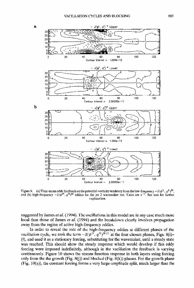
Superscript M+L corresponds to the low frequencies plus the mean value. The second two terms on the right-hand side (r.h.s) of Eq. (9) are shown in Figs. 9(a) and (b), which are the feedbacks by the low- and high-frequency eddies, respectively, onto the mean flow. The high-frequency forcing in the lower layer is dominant. The low-frequency forcing in the lower layer also shows a weaker quadrupole of reversed sign and smaller zonal scale. In the upper-layer the low-frequency eddy feedback also opposes the high-frequency feedback over the wavemaker. The two terms on the r.h.s. of (10) vary at each phase of the cycle. The high-frequency forcing terms from (9) and (10) are shown combined in Figs. 8(i j (1). The persistent structure of the high-frequency eddy terms and the opposite sign (and equal magnitude in the upper-layer) of the low-frequency forcing, suggest that the high- frequency eddies do not drive the flow through the entire low-frequency oscillation cycle as


25 20 15 10 5

a

I

5 0


- J ( V . a") " Lower .. . . , 30 25 20 15 10 5 0 0 20 40 60 80 100 120

Contour lntervoi = 2.00000e- 11

Figure 9. (a)Tirne-rneaneddy feedbackon the potential-vorticity tendency from the low-frequency -J(GL, qL)M, and (b) high-frequency -J(GH, qH)M eddies for the jet 2 wavemaker run. Units are s-~. See text for further

explanation.

suggested by James et al. (1994). The oscillations in this model are in any case much more local than those of James et al. (1994) and the breakdown clearly involves propagation away from the region of active high-frequency eddies.

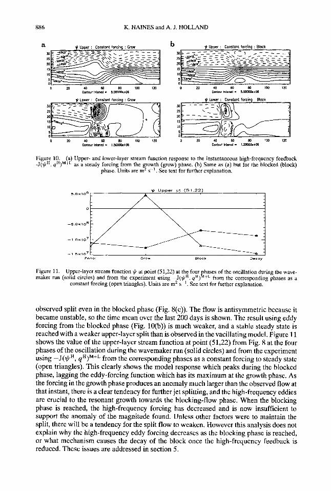
In order to reveal the role of the high-frequency eddies at different phases of the vacillation cycle, we took the term -J(lCrH, qH)M+L at the four chosen phases, Figs. 8(i)- (l), and used it as a stationary forcing, substituting for the wavemaker, until a steady state was reached. This should show the steady response which would develop if this eddy forcing were imposed indefinitely, although in the vacillation the feedback is varying continuously. Figure 10 shows the stream function response in both layers using forcing only from the the growth (Fig. 80)) and blocked (Fig. 8(k)) phases. For the growth phase (Fig. lO(a)), the constant forcing forms a very large-amplitude split, much larger than the


t Upper : Constont lorcing : Block b j , Upper : Constont forcing : Grow a

0 20 4a w en 1w 120 0 20 4a €4 80 tw 120 Contour IntwwI I 5.WOoat06 Contovr hltlnnl I 5.wwo.to6

+ Lower : Constont forcing : Grow 30 25 20 15 10 5 0 0 20 40 €4 M) IM 120

9 ~ower : Constant forcing : Block

0 20 4 w en tw 120 Cmtwr Intermi - I.%XX&+O6

Figure 10. (a) Upper- and lower-layer stream function response to the instantaneous high-frequency feedback - J ( + H , qH)M'L as a steady forcing from the rowth (grow) phase. (b) Same as (a) but for the blocked (block)

phase. Units are m' s-'. See text for further explanation.

Upper at (51,22) 5 . O X 1 O 6 -

a - -

- 1 5 x 1 0 ~ - Z 0 " d W l o c k

Figure 11. Upper-layer stream function + at point (51,22) at the four hases of the oscillation during the wavemaker run (solid circles) and from the experiment using -J($rH, yH)R+L from the corresponding phases as a

constant forcing (open triangles). Units are m2 s-'. See text for further explanation.

observed split even in the blocked phase (Fig. 8(c)). The flow is antisymmetric because it became unstable, so the time mean over the last 200 days is shown. The result using eddy forcing from the blocked phase (Fig. lO(b)) is much weaker, and a stable steady state is reached with a weaker upper-layer split than is observed in the vacillating model. Figure 11 shows the value of the upper-layer stream function at point (51,22) from Fig. 8 at the four phases of the oscillation during the wavemaker run (solid circles) and from the experiment using -J(@H, qH)MfL from the corresponding phases as a constant forcing to steady state (open triangles). This clearly shows the model response which peaks during the blocked phase, lagging the eddy-forcing function which has its maximum at the growth phase. As the forcing in the growth phase produces an anomaly much larger than the observed flow at that instant, there is a clear tendency for further jet splitting, and the high-frequency eddies are crucial to the resonant growth towards the blocking-flow phase. When the blocking phase is reached, the high-frequency forcing has decreased and is now insufficient to support the anomaly of the magnitude found. Unless other factors were to maintain the split, there will be a tendency for the split flow to weaken. However this analysis does not explain why the high-frequency eddy forcing decreases as the blocking phase is reached, or what mechanism causes the decay of the block once the high-frequency feedback is reduced. These issues are addressed in section 5.


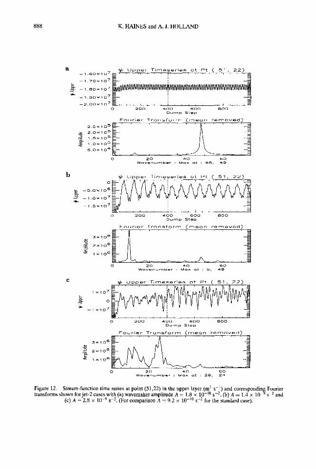
(b) Nonlinear aspects A further facet of the low-frequency oscillation is revealed by varying the amplitude

of the wavemaker. Figure 12 shows three time series of @ at the same position as in Fig. 7. Figure 12(a) is for a wavemaker with amplitude reduced by a factor of 5. The wavemaker eddies are clearly visible but there is little sign of the low-frequency oscillation. Figure 12(b) is for a wavemaker with amplitude increased by a factor of 1.5 over that shown in Fig. 7 . In this case the low-frequency oscillation period has decreased from 31 days to 24 days. If the wavemaker amplitude is further increased the flow rapidly develops other oscillation frequencies and the response begins to be chaotic; this is shown in Fig. 12(c) for the amplitude increased by a factor of 3 from the original (A = 2.8 x lop9 s-’).

This sensitivity to the wavemaker amplitude is consistent with an instability mechanism being responsible for the breakdown of blocking in the channel. If the amplitude of the split jet is insufficient (weak wavemaker), the low-frequency oscillation is absent. If the high-frequency eddies are stronger the split jet reaches the amplitude required for instability more rapidly, and therefore block decay sets in leading to an increase in block- decay-cycle frequency. These results lead us to perform the stability analyses reported in the next section.

5. LOW-FREQUENCY OSCILLATIONS AND STABILITY

The full stability properties of non-zonal flows such as those formed here are difficult to study, and there are few general principles which can be used for guidance. During the low-frequency oscillation cycles the flow is never steady making conventional stability analyses ambiguous, see Andrews (1984). The proper analysis method for such situations is error growth theory which can be studied through the development of singular vectors, e.g. Fanell (1985). We chose to avoid these difficulties and opted instead for a greatly simplified analysis of the zonal-flow stability of the different flow phases and, as will be seen, this appears to be sufficient to explain the low-frequency oscillation behaviour.

(a) Stability analysis To assess the stability of the low-frequency component of the channel flows in Fig. 8,

the meridional stream-function profile at each x position and at each time t , was analysed in the following eigenvalue problem:

where Ui are the zonal-velocity components of layers i of the low-pass filtered fields at a particular time and x position, with corresponding potential-vorticity gradients d Qi /dy ; 4; are the meridional eigenvectors and c are the zonal phase-speed eigenvalues. These equations come from linearizing (1) about a zonal flow, and seeking solutions of the form

Several simplifications have been made for this analysis. The wavemaker, friction and all the zonal derivative terms have been neglected, so that each meridional cross-section in the channel is analysed as if it were a zonal flow. Such an analysis will not, of course, give the exact stability modes or growth rates but, to the extent that north-south gradients

p/,7i = 4i (y)eik(x-c‘).


Upper Timeseries at Pt ( 51, 2 2 ) . ' I " . ~ " ' I ' ~ " ' ' '

a

- 1 . 7 0 x 1 o 7 % a

-L

1 . 8 O X 1 0 '

- 1 . s o x 107

- -2 .00x107 0 200 400 600 800

Durnp Step

Fo.dr;er T r u r i s f v r r r t ( r n e u r i rernoved)

0 20 4 0 ti0 W a v e n u m D e r . M a x at . 48. 49

b + Upper Timeseries a t Pt ( 5 1 , 22) 0

b -5.ox106 a a =) --1.oX1o7

- 1 . 5 x 1 0 7 -+

0 zoo 400 600 aoo D u m p Step

3 x 1

2 x 1

1 X l

Fourier Transform ( m e a n removed)

06 ~~1 0 20 40 6 0

Wavenumber ! M a x at : 9. 48

C + Upper Timeseries at Pt ( 51. 2 2 )

1 z2

0 a 0. 3 -L

-1 X I 0 7

0 200 400 600 aoo Dump Step

Fourier Transform ( m e a n removed)

3 x 1 O6 w 3 .- - - 2 x 1 0 6

e 4 1 x 1 0 6

0 2 0 40 60 Wovenumber : Max at : 26. 2 4

Figure 12. Stream-function time series at point (51,22) in the upper layer (m2 s-') and correspondin Fourier transforms shown for jet-2 cases with (a) wavemaker amplitude A = 1.8 x lo-'' s-', (b) A = 1.4 x I d s-' and

(c) A 2.8 x s-'. (For comparison A = 9.2 x lo-'' s-' for the standard case).


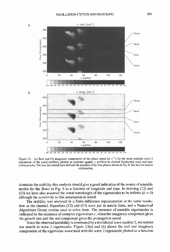
Figure 13. (a) Real and (b) imaginary components of the phase speed (m s-l) for the most unstable wave 2 eigenmode of the zonal problem, plotted as contours against x position in channel (horizontal axis) and time (vertical axis). The four horizontal lines indicate the position of the four phases shown in Fig. 8. See text for further

explanation.

dominate the stability, this analysis should give a good indication of the source of unstable modes for the flows in Fig. 8 as a function of longitude and time. In deriving (12) and (13) we have also assumed the zonal wavelength of the eigenmodes to be infinite ( k = 0) although the sensitivity to this assumption is tested.

The stability was analysed in a finite-difference representation at the same resolution as the channel. Equations (12) and (13) were put in matrix form, and a Numerical Algorithms Group routine used to solve them. The presence of unstable eigenmodes is indicated by the existence of complex eigenvalues c, when the imaginary component gives the growth rate and the real component gives the propagation speed.

Since the observed instability is dominated by a meridional wave number 2, we restrict our search to wave 2 eigenmodes. Figure 13(a) and (b) shows the real and imaginary components of the eigenvalue associated with the wave 2 eigenmode plotted as a function


of zonal position and time. This method of display shows exactly at what zonal positions and at what times the flow becomes unstable. The times of the four phases shown in Fig. 8 are indicated. The first thing to note is that there is a genuine change during the oscillation from periods when the flow is stable at all longitudes, to periods when instability is quite marked. Instability first appears during the growth stage of the oscillation with the unstable longitudes located around and upstream of the maximum split in the upper-layer jet stream. It appears to be the region of the westerly flow in the lower layer, upstream of the upper-layer split, which is responsible for the instability. If the maximum growth rates of the unstable eigenmodes are calculated from Im(c) by estimating a suitable k value, an e-folding time-scale of a few days results. The real component of the eigenvalue for these unstable modes is always negative, indicating upstream propagation with a typical speed of around 10 m s-'. This is consistent with the description of the breakdown of blocking in section 4, in which a large-scale wave travels upstream from the blocking region.

If any of the steady blocking responses in section 3 are analysed, it is found that the zonal-flow component at all longitudes remains stable, i.e. no complex eigenvalues exist. This is good evidence that the breakdown of the blocking phase in the channel is initiated by large-scale instability. The instabilities shown in Fig. 13 are of mixed barotropic/baroclinic type as can be shown by separating the appropriate zonal flows into their barotropic and baroclinic components. Neither component is unstable in its own right, and the instability relies on both vertical and horizontal shears in order to develop. This is consistent with the fact that in section 3 many high-amplitude blocks were formed which were perfectly stable. The introduction of meridional shear into the original jet causes the flow to become locally unstable whenever a large amplitude block is superimposed.

(b) Energy diagnostics In this section we use an analysis of energy conversions similar to that presented

by Higgins and Schubert (1994). Following some mathematics, for which refer to their appendix, the following equation for the time tendency of the low-frequency kinetic energy i3 (vL.vL/2) / a t is obtained,

a - ( K E ~ ) = C ( K E ~ , K E ~ ) + C ( K E ~ , K E ~ ) + C ( P E ~ , K E ~ ) + R + F , at (14)

where K E denotes kinetic and P E potential energy, and:

C ( K E M , K E L ) = -(CLVL.k x vM)

represents a barotropic-energy conversion from the mean flow to the low-frequency kinetic energy;

C ( K E H , K E L ) = (CHVH.k x vL)

represents a barotropic-energy conversion from the high-frequency to the low-frequency kinetic energy;

represents a conversion from the low-frequency potential to low-frequency kinetic energy;

F = vL.(-(& + S(x))vL + vV2vL)

C ( P E L , K E L ) = -(f"@Lv.vL)

is the component due to friction and R is the sum of all the remaining terms which are not included elsewhere. Note that (...) indicates a sum over a layer and v is the geostrophic velocity in all terms except v .vL .

VACILLATION CYCLES AND BLOCKING 89 1

We use a slightly different notation to Higgins and Schubert (1994) in the superscripts (our mean M is their seasonal mean S and our high frequency H is their bandpass frequency B); also we do not use a composite average over various events as they did. We simply look at the balances for one oscillation as the behaviour here is more regular than their GCM data. The divergence term V.vL is calculated using the vorticity tendency equation. Our R term has only been calculated approximately and, like Higgins and Schubert, we ignore any terms containing vertical velocity w ; the balance appears to be good even neglecting these.

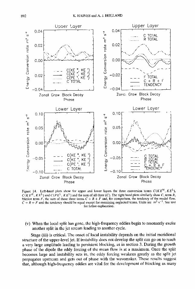
Figure 14 shows these terms as they vary through the vacillation cycle. The upper plots are for the upper layer, the lower plots for the lower layer. The left-hand plots show the three conversion terms plus their sum, representing the total conversion term. The right- hand plots show this total together with the terms R and F , the total sum of all the r.h.s. of (14) and, finally, a direct estimate of the left-hand side tendency in K E L , calculated from the model.

We first consider the balances in the lower layer. The bottom-left plot in Fig. 14 shows that the dominant term is the barotropic conversion from high frequencies. This involves a large peak during the growth phase, indicating that the high frequencies are responsible for the growth of the anomaly. In the blocked phase the contribution from this term is approaching zero and it becomes weakly negative in the decay phase. The bottom-right plot shows the contributions from the other terms to the total balance. The high-frequency conversion term is much larger in magnitude than the total conversion term; the difference comes from the friction, which is negative at all periods throughout the cycle, and the residual R terms, of which the dominant component is (vL.(CHk x v ~ ) ~ ) . Note that Higgins and Schubert found their R term to be dominated by the term (vL.(CLk x v ~ ) ~ ) .

Now we consider the upper layer. The conversion terms are different in this layer mainly due to the weaker effects of the high frequencies. The upper-left plot of Fig. 14 shows that conversion from high frequencies now makes the smallest contribution. Instead, the conversion from P E L is the dominant term, and peaks just before the blocking peak. This is consistent with baroclinic instability setting in at that time, converting P E to K E . The conversion from K E M also supplements this term, with a peak just after the block peak indicating a barotropic-instability component. In the top-right plot, variations in total K E L production is shown to mirror this conversion term, but with variation about zero due to the friction which increases a little during the decay phase of the cycle. The R term in the upper-layer is negligible in the balance. Comparison of the sum of the terms calculated with the energy tendency observed, shows that we have captured the shape well, with a slight underestimation at all points due to the terms neglected.

(c ) Summary We are now in the position to describe schematically the stages and the physical

(i) Resonant excitation of anticyclonelcyclone dipole by feedback from high-frequency eddies.

(ii) This dipole anomaly becomes superimposed on the upper-level jet approaching from upstream.

(iii) If sufficient meridional shear is already present in the upper-level jet stream the presence of the local dipole anomaly can induce local instability after the split reaches a certain amplitude.

(iv) The split jet starts to be broken down by large-scale baroclinic-barotropic instability which transfers energy to a large-scale westward-propagating wave.

mechanisms leading to the low-frequency blocking vacillations observed.


C TOTAL ___._._ R TOTAL

0 0 x -0.05

Upper Layer

ffl

E O*04.

Upper Layer

m

__ . .___ R TOTAL "E

1 - - - C I K E " KE 4 1 - C KE ''; KE _ . . . _ _ _ C P E ' , K E ' -0.02

C TOTAL

W -0.04; Zonal G r o w Block Decay

Phase

Lower Layer

m O.lol-----l N

E a, 0.05 2

'v, 0.00

&

C 0

a, > c 0 0 x

a, c W

L

-0.05 F

-0.10

Zonol Grow Block Decay Phase

Lower Layer

m 0.1°!7----

- - - C(KE ", KE ') __ C(KE ", KE ') _ . _ _ _ _ . C(PE ', KE ')

C TOTAL

Zonal G r o w Block Decoy Phase

Zonal Grow Block Decay Phase

Figure 14. Left-hand plots show for upper and lower layers the three conversion terms C ( K E M , K E L ) , C ( K E H , K E L ) and C ( P E L , K E L ) and the sum of all three (C). The right hand plots similarly show C , term R, friction term F, the sum of these three terms C + R + F and, for comparison, the tendency of the model flow. C + R + F and the tendency should be equal except for remaining neglected terms. Units are m2 s - ~ . See text

for futher explanation.

(v) When the local split has gone, the high-frequency eddies begin to resonantly excite another split in the jet stream leading to another cycle.

Stage (iii) is critical. The onset of local instability depends on the initial meridional structure of the upper-level jet. If instability does not develop the split can go on to reach a very large amplitude leading to persistent blocking, as in section 3. During the growth phase of the dipole the eddy forcing of the mean flow is at a maximum. Once the split becomes large and instability sets in, the eddy forcing weakens greatly as the split jet propagates upstream and gets out of phase with the wavemaker. These results suggest that, although high-frequency eddies are vital for the development of blocking as many


other authors have shown, it may be the meridional structure of the upper-level jet which determines the persistence and strength of the block.

6. DISCUSSION AND CONCLUSIONS

This paper reports results of experiments with a baroclinic channel model in which a low-frequency, blocking-like vacillation is produced. The excitation, splitting-jet phase of the vacillation is caused by vorticity fluxes from high-frequency transient eddies, but the response is largely a neutral stationary Rossby wave. As the split-jet flow evolves, it enables the high frequencies to increase their influence on the large-scale flow with a positive feedback effect. The breakdown phase is caused by large-scale mixed barotropic- baroclinic instability which sets in when the split amplitude becomes large enough, but only if there is sufficient meridional shear in the upper-layer zonal jet stream. Without meridional shear, a large-amplitude stable block is excited by the high-frequency eddies.

The development of local instability, such as that reported here, has been found by other investigators studying blocking-like flows. The work of Helfrich and Pedlosky (1993,1995) is an example in which local instability in a dipole soliton develops if the zonal flow on which the soliton grows is close to being baroclinically unstable. James ef al. (1994) performed empirical orthogonal function analyses on the zonal wind of two 100- year integrations of a simplified GCM. They identified a low-frequency circulation in the phase space of the principal components (PCs) with a period of 150 days. By calculating the feedback of normal-mode baroclinic life cycles at various phases of the cycle, they showed a tendency to partially drive the zonal state along an anticlockwise trajectory in the phase-space. All baroclinic life cycles increased the PC1 value, but some other mechanism is needed to reduce the PC1 amplitude and complete the circuit.

Our case is similar, with the feedback from the high-frequency eddies pushing the flow towards the block stage, and the extra mechanism required to complete the cycle is instability, evidence of which is provided by a local zonal-flow stability analysis and energy diagnostics. This instability also provides a mechanism for the propagation of wave information away from the region of splitting, which could contribute to the ultra- low-frequency variability of James et al. (1994), run A.

Future work will involve searching for evidence of this behaviour in more sophisti- cated models and in observed data. It has been known for some time that high-frequency eddies can reinforce atmospheric blocks, but little is known of why this behaviour does not always occur nor continues indefinitely. The evolution of the large-scale flow to become unstable, or affect the feedback mechanism in some way, may possibly provide further in- sights into the behaviour of low-frequency variance in the atmosphere. It could be that the jet stream evolves between different states which support different types and amplitudes of local anomaly. For instance, if the atmospheric jet was in a state similar to our jet 1 case, then a persistent blocked flow could be excited. The jet could then slowly shift towards a regime where the anomaly would become unstable and breakdown. If this transition was slow, then the flow could remain marginally stable for a period of time, which may result in an upstream propagation as seen in our model, consistent with findings from case studies. An improved predictability and understanding of blocking events would undoubtedly help reduce weather forecasting errors, especially in the medium range.

ACKNOWLEDGEMENTS

The authors would like to thank the UK Universities Global Atmospheric Modelling Programme (UGAMP) and NERC (Grant : GST/02/804) for providing the funding for


this work, and the computing personnel at the University of Edinburgh for maintaining the facilities to make this research possible. Useful discussions with Chris Thorncroft of Reading University are also acknowledged.

Andrews, D. G.

Branstator, G.

Dole. R. M.

Edmon, H. J., Hoskins, B. J. and McIntyre, M. E.

Ferranti, L., Molteni, F. and Palmer, T. N.

Farrell, B. F.

Flierl, G. R. and Haines, K.

Green, J. S. A.

Haines, K.

Haines, I(. and

Haines, K. and Marshall, J.

Helfrich, K. R. and Pedlosky, J.

Malanotte-Rizzoli, P.

Higgins, R. W. and Schubert, S. D.

Hoskins, B. J.

Hoskins, B. J., James, I. N. and

Hoskins, B. J., McIntyre, M. E. and

Illari, L.

James, P. M., Fraedrich, K. and

White, G. H.

Robertson, A. W.

James, I. N.

McWilliams, J. C.

Mo, K. C., and Ghil, M.

Mullen, S. L.

Plaut, G . and Vautard, R.

Plumb, R. A.

1984

1992

1986

1989

1980

1994

1985

1994

1977

1994

1991

1987

1993

1995

1994

1983

1983

1985

1984

1994

1980

1988

1986

1994

1990

REFERENCES On the stability of forced non-zonal flows. Q. J. R. Meteorol. Soc.,

110,657-662 The maintenance of low-frequency atmospheric anomalies. J.

Atmos. Sci., 49,1924-1945 Persistent anomalies of the extratropical northern hemisphere win-

ter time circulation: Structure. Mon. Weather Rev., 114,178- 207

Life cycles of persistent anomalies. Part I: Evolution of 500 mb height fields. Mon. Weather Rev., 117, 177-211

Eliassen-Palm cross sections for the troposphere. J. Amos. Sci., 37,2600-2616

Impact of localized tropical and extratropical SST anomalies in ensembles of seasonal GCM integrations. Q. J. R. Meteorol.

Transient growth of damped baroclinic waves. J. Atmos. Sci., 42,

The decay of modons due to Rossby wave radiation. Phys. Fluids,

The weather during July 1976 : Some dynamical considerations of the drought. Weather, 32,120-128

Low-frequency variability in atmospheric middle latitudes. Sur- veys Geophys., 15,1-61

Isolated anomalies in westerly jet streams: A unified approach. J. Atmos. Sci., 48,5 10-526

Eddy-forced coherent structures as a prototype of atmospheric blocking. Q. J . R. Meteorol. SOC., 113,681-704

Time-independent isolated anomalies in zonal flows. J. Fluid Mech., 251,377-409

Large-amplitude coherent anomalies in baroclinic zonal flows. J. Atmos. Sci., 52,1615-1629

Simulated life cycles of persistent anticyclonic anomalies over the North Pacific: Role of synoptic-scale eddies. J. Atmos. Sci., 51,3238-3260

‘Modelling of transient eddies and their feedback on the mean flow’. In Large-scale dynamicalprocesses in the atmosphere. Eds. B. J. Hoskins and R. P. Pearce, Academic Press, London, UK

The shape, propagation and mean-flow interaction of large-scale weather systems. J. Atmos. Sci., 40, 1595-1612

On the use and significance of isentropic potential vorticity maps. Q. J. R. Meteorol. SOC., 111,877-946

A diagnostic study of potential vorticity in a warm blocking anticyclone. J . Atmos. Sci., 41,3518-3526

Wave-zonal-flow interaction and ultra-low-frequency variability in a simplified global circulation model. Q. J. R. Meteorol. SOC., 120,1045-1067

An application of equivalent modons to atmospheric blocking. Dyn. Atmos. Ocean. 5 , 4 3 4 6

Cluster analysis of multiple planetary flow regimes. J. Geophys. Res., 93,10927-10951

The local balances of vorticity and heat for blocking anticyclones in a spectral general-circulation model. J. Atmos. Sci., 43, 1406-1 441

Spells of low-frequency oscillations and weather regimes in the Northern Hemisphere. f. Amos. Sci., 51,21&236

A nonacceleration theorem for transient quasi-geostrophic eddies on a three-dimensional time-mean flow. J. Atmos. Sci., 47, 1825-1836

SOC., 120,1613-1645

2718-2727

6,3489-3497


Shutts, G. J.

Stone. P.

Thorncroft, C. D., Hoskins, B. J.

Vautard. R. and McIntyre, M. E.

Vautard, R. and Legras, B.

Vautard, R., Pires, C. and Plaut, G.

1983

1986

1972

1993

1990

1988

1996

The propagation of eddies in diffluent jet streams: Eddy vorticity of ‘blocking’ flow fields. Q. J. R. Meteorol. Soc., 109,737-761

A case study of eddy forcing during an Atlantic blocking episode. Adv. Geophys., 29,135-162

A simplified radiative-dynamical model of the static stability of rotating atmospheres. J. Atmos. Sci., 29,405-418

’ h o paradigms of baroclinic-wave life-cycle behaviour. Q. J. R. Meteorol. SOC., 119, 17-56

Multiple weather regimes over the North Atlantic: Analysis of precursors and successors. Mon. Weather Rev., 118, 2056- 2081

On the source of low-frequency variability. Part 11: Nonlinear equi- libration of weather regimes. J. Atmos. Sci., 45, 2845-2867

Long-range atmospheric predictibility using space-time principal components. Mon. Weather Rev., 124,288-307

Documents

Vacillation cycles and blocking in a channel