Embed Size (px)
Citation preview

Vacuum Science and Technology
for Particle Accelerators
Yulin LiCornell University, Ithaca, NY
Xianghong LiuSLAC National Accelerator Laboratory
Albuquerque, New MexicoJune 17-28, 2019

About Your Instructors
• Yulin Li- Vacuum Scientist ([email protected])
- Cornell Laboratory for Accelerator-based Sciences and Educations (CLASSE)
- Self-taught vacuum practitioners, starting as surface scientists
- As research staff members at CLASSE over 25 years overseeing all aspect of vacuum operations,
designs and R&D
• CLASSE – A Research Center on Cornell’s Ithaca Campus- Primary funding – NSF, with additional funding from DOE
- Cornell Electron Storage Ring (CSER): 780-m, 500-mA, 5-GeV
- Cornell High Energy Synchrotron Sources (CHESS) – A SR-user facility w/ 12 experimental
stations
- CBETA
- Center for Bright Beams
- Superconducting RF researches
USPAS - Vacuum Fundamentals

About Your Instructors
• Xianghong Liu- Vacuum Scientist ([email protected])
- SLAC National Accelerator Laboratory (2018.09 – present)
- CLASSE, Cornell University (2004.10 - 2018.8)
- Design, manufacturing, and operation of accelerator vacuum systems
• SLAC National Accelerator Laboratory- Linac Coherent Light Source (LCLS)
- LCLS II
- Facility for Advanced Accelerator Experimental Tests (FACET)
- Stanford Positron Electron Asymmetric Ring (SPEAR3)
USPAS - Vacuum Fundamentals

USPAS Vacuum (June 17-21, 2019) 4
Special thanks go to Mr. Lou Bertolini of LLNL, who shared ~1000 slides with me
from his previous USPAS Vacuum lectures.
Thanks also go to many of my colleagues from other accelerator facilities, who
provided valuable information.
Many vacuum product companies graciously supported with their presentations,
detail technical information and demo products.
Most importantly, we are grateful for CLASSE-Cornell’s and SLAC’s supports, and
for NSF’s continuous support in our researches.
Acknowledgements
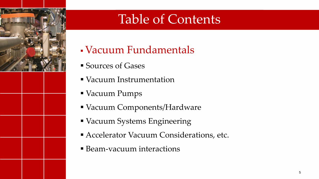
Vacuum Fundamentals
Sources of Gases
Vacuum Instrumentation
Vacuum Pumps
Vacuum Components/Hardware
Vacuum Systems Engineering
Accelerator Vacuum Considerations, etc.
Beam-vacuum interactions
Table of Contents
5

6
Schedule & GradingMonday – Fundamental (Session 1) and Gas Sources (Session 2)
Tuesday – Instruments (Session 3) and Pumps (Session 4)
Wednesday – Pumps (cont.) & Vacuum Hardware and Fabrications (Session 5)
Thursday – System Engineering (Session 6.1) and Vacuum Calculations (1D and MolFlow demonstrations)
Friday – System Integration (Session 6.2) and Beam Vacuum Interactions (Session 7)
There are daily homework, must submitted by Friday (if not earlier), for grade students
No final exam. Grade will be based on class participation (60%) and homework (40%)
USPAS Vacuum (June 17-21 2019)
Demos: (1) Tuesday 4pm (MKS Instruments); (2) Wednesday 4pm (Agilent Vacuum)

SESSION 1: VACUUM FUNDEMENTALS
• Vacuum definition and scales
• Gas properties and laws
• Gas flow and conductance
7

8
The Basics
USPAS Vacuum (June 17-21 2019)

What is a Vacuum ?
• A vacuum is the state of a gas where the density of the
particles is lower than atmospheric pressure at the earth's
surface
• Vacuum science studies behavior of rarefied gases,
interactions between gas and solid surfaces (adsorption and
desorption), etc.
• Vacuum technology covers wide range of vacuum pumping,
instrumentations, material engineering, and surface
engineering
9USPAS - Vacuum Fundamentals

10
Accelerator Vacuum – highly interdisciplinary
Accelerator Vacuum
Science and Technology
Physics
Fluid Mechanics
Mechanical Engineering
Chemistry
Metallurgy
Mathematics
Surface Sciences
Electronics Molecular Thermodynamics
USPAS Vacuum (June 17-21, 2019)

11
Units, Scales & Molecular Densities
SI Pressure Unit: Pascal (Pa) = N/m2
Other commonly used units: Torr (mmHg) = 133.3 Pa
mbar = 100 Pa = 0.75 Torr
USPAS Vacuum (June 17-21, 2019)

12
Extreme High Vacuum
(P < 10-11 torr)Photo-cathode electron sources (Cornell, JLab, BNL,),
High intensity ion accelerators (RHIC, GSI, …) etc.
Ultra-High Vacuum
(10-9 to 10-11 torr)Storage rings, e-/e+ colliders, surface sciences, etc.
High Vacuum
(10-3 to 10-9 torr)Device fabrications, medical accelerators, LINACs,
mass spectrometry, SEM, etc.
Medium & Low
Vacuum
Cryo insolation vacuum, thin film coating, vacuum
furnaces, beam welders, etc.
Example Vacuum Applications
USPAS Vacuum (June 17-21, 2019)

13
Dry Air Composition and Molecular MassConstituent Molecular
Mass
Molecular
Mass in Air
N2 78.08 28.02 21.88
O2 20.95 32.00 6.704
Ar 0.934 39.94 0.373
CO2 0.037 44.01 0.016
H2 0.5 2.02 ---
Ne 18.2 20.18 ---
He 5.24 4.00 ---
Kr 1.14 83.8 ---
Xe 0.087 131.3 ---
CH4 2.0 16.04 ---
N2O 0.5 44.01 ---
Total 28.97
Volume Content
Percent ppm
USPAS Vacuum (June 17-21, 2019)

14
Water Vapor in Air
• Water has most detrimental effects in a clean vacuum system
• Water molecular mass:
18.08 kg/mole
(‘humid’-air is less dense!)
• Water content in air is usually expressed in
relative humidity ():
∅ =𝑃𝑃𝑤
𝐻2𝑂
𝑃𝑃𝑤_𝑠𝑎𝑡𝐻
2𝑂 x 100%
USPAS Vacuum (June 17-21, 2019)

15
Gas Properties & Laws
USPAS Vacuum (June 17-21, 2019)

16
Kinetic Picture of an Ideal Gas
1.The volume of gas under consideration contains a large
number of molecules and atoms – statistic distribution applies
2.Molecules are far apart in space, comparing to their individual
diameters.
3.Molecules exert no force on one another, except when they
collide. All collisions are elastic (i.e. no internal excitation).
4.Molecules are in a constant state of motion, in all direction
equally. They will travel in straight lines until they collide with
a wall, or with one another
USPAS Vacuum (June 17-21, 2019)

17
Maxwell-Boltzmann Velocity Distribution
2
22
2/3
2/1 2
2 vkT
m
evkT
mN
dv
dn
– velocity of molecules (m/s)
dn – number of molecules with between and + d
N – the total number of molecules
m – mass of molecules (kg)
k – Boltzmann constant, 1.3806503×10⁻²³ m2 kg s-2 K-1
T – temperature (Kelvin)
USPAS Vacuum (June 17-21, 2019)

18
A Close Look at Velocity Distribution
1.0
0.8
0.6
0.4
0.2
0.0
dn
/dv (
arb
. u
nit)
1400120010008006004002000
Velocity (m/s)
vp vavg
vrms
Air @ 25°C
• Most probable velocity (m/s):
• Arithmetic mean velocity:
• Root Mean Squared velocity:
moleMT
mkT
pv 44.1282
pmkT
avg vv 128.18
pmkT
rms vv 225.13
Velocity depends on mass and temperature, but independent of pressure
USPAS Vacuum (June 17-21, 2019)

19
=1.667 (atoms); 1.40 (diatomic); 1.31 (triatomic)
Speed of Sound in Ideal Gases
m
kTPvsound
where Vp CC
is the isentropic expansion factor
Mono-atomic
Di-atomic
Tri-atomic
vp/vsound 1.10 1.19 1.24
vavg/vsound 1.24 1.34 1.39
vrms/vsound 1.34 1.46 1.51
Though not directly related, the characteristic gas speeds are close to the speed of sound in ideal gases.
USPAS Vacuum (June 17-21, 2019)

20
Molecules Move Faster at Higher Temperatures
USPAS Vacuum (June 17-21, 2019)

21
Lighter Molecules Move Faster
USPAS Vacuum (June 17-21, 2019)

22
Maxwell-Boltzmann Energy Distribution
kT
E
ekT
EN
dE
dn 2
23
21
2/1
2
• Average Energy: Eavg = 3kT/2• Most probable Energy: Ep = kT/2
Neither the energy distribution nor the average energy of the gas is a function of the molecular mass. They ONLY depend on temperature !
USPAS Vacuum (June 17-21, 2019)

23
Mean Free Path
The mean free path is the average distance that a gas molecule can
travel before colliding with another gas molecule.
Mean Free Path is determined by:
size of molecules, density (thus pressure and temperature)
USPAS Vacuum (June 17-21, 2019)

24
Mean Free Path Equation
Pd
kT
nd 2
0
2
0 22
1
- mean free path (m)
d0 - diameter of molecule (m)
n - Molecular density (m-3)
T - Temperature (Kevin)
P - Pressure (Pascal)
k - Boltzmann constant, 1.38×10⁻²³ m2 kg s-2 K-1
USPAS Vacuum (June 17-21, 2019)

25
Mean Free Path – Air @ 22C
)(
005.0
)(
67.0)(
TorrPPaPcm
P (torr) 760 1 10-3 10-6 10-9
(cm) 6.6x10⁻⁶ 5.1x10⁻³ 5.1 5100 5.1x10⁶
For air, average molecular diameter = 3.74 x10⁻⁸ cm
USPAS Vacuum (June 17-21, 2019)

26
Properties of Some Gases at R.T.
Properties H2 He CH4 Air O2 Ar CO2
avg (m/s) 1776 1256 628 467 444 397 379
d0(10-10 m)
2.75 2.18 4.19 3.74 3.64 3.67 4.65
atm
(10-8 m)
12.2 19.4 5.24 6.58 6.94 6.83 4.25
atm
(1010 s-1)
1.46 0.65 1.20 0.71 0.64 0.58 0.89
avg : mean velocity
d0 : molecular/atomic diameter
atm : mean free length at atmosphere pressure
atm : mean collision rate, atm = avg / atm
USPAS Vacuum (June 17-21, 2019)

27
Particle Flux
Particle Flux – rate of gas striking a surface or animaginary plane of unit area
Kinetic theory shows the flux as:
m
kTnnsm avg
24
1)( 12
where n is the gas density
Particle flux is helpful in understanding gas flow,
pumping, adsorption and desorption processes.
USPAS Vacuum (June 17-21, 2019)

28
Particle Flux – Examples
P n Particle Flux (m-2s-1)
(torr) m-3 H2 H2O CO/N2 CO2 Kr
760 2.5x1025 1.1x1028 3.6x1027 2.9x1027 2.3x1027 1.7x1027
10-6 3.2x10¹⁶ 1.4x10¹⁹ 4.8x10¹⁸ 3.8x10¹⁸ 3.1x10¹⁸ 2.2x10¹⁸
10-9 3.2x10¹³ 1.4x10¹⁶ 4.8x10¹⁵ 3.8x10¹⁵ 3.1x10¹⁵ 2.2x10¹⁵
Typical atomic density on a solid surface: 5.0~12.0x10 18 m -2
Thus monolayer formation time at 10 -6 torr: ~ 1-sec !
A commonly used exposure unit: 1 Langmuir = 10-6 torrsec
USPAS Vacuum (June 17-21, 2019)

29
The Ideal Gas Law
zmP 2
molecules striking a unit area, with projected velocity of z exert an impulse, or
pressure, of:
Integrate over all velocity, based on kinetics,
2
31
rmsnmP
The average kinetic energy of a gas is:
kTmE rms 232
21
(A)
(B)
Equations (A) and (B) results in the Ideal Gas Law:
nkTP USPAS Vacuum (June 17-21, 2019)

30
Gas Laws
Charles’ Law
Volume vs. temperature
Boyle’s Law
Pressure vs. Volume
Avogadro’s Law
Volume vs. Number of molecules
All these laws derivable from the Ideal Gas Law They apply to all molecules and atoms, regardless of their sizes
USPAS Vacuum (June 17-21, 2019)

31
Charles’ Law
2
2
1
1
T
V
T
V
(N, P Constant)
USPAS Vacuum (June 17-21, 2019)

32
Boyle’s Law
2211 VPVP
(N, T Constant)
USPAS Vacuum (June 17-21, 2019)

33
Finding volume of a vessel with Boyle’s Law
Boyle’s Law can also be used to expend gauge calibration range via expansion
USPAS Vacuum (June 17-21, 2019)

34
Avogadro’s Law
Equal volumes of gases at the same temperature and pressure contain the same number of
molecules regardless of their chemical nature and physical properties
2
2
1
1
N
V
N
V (P, T Constant)
USPAS Vacuum (June 17-21, 2019)

35
Avogadro’s Number
At Standard Temperature and Pressure (STP, 0C at 1 atmosphere), a mole of ideal gas has a volume of Vo, and contains NA molecules and atoms:
NA = 6.02214×10²³ mol −1
Vo = 22.414 L/mol
Definition of mole: (to be obsolete in new SI system!!)the number of atoms of exact 12-gram of Carbon-12
Among other changes in the new SI, NA will be set to be an exact value as shown above, and mole will be redefined.
USPAS Vacuum (June 17-21, 2019)

36
Partial Pressure – The Dalton’s Law
The total pressure exerted by the mixture of non-reactive gases equals to the sum of the
partial pressures of individual gases
ntotal pppP ...21
where p1, p2, …, pn represent the partial pressure of each component.
kTnnnP ntotal )...( 21
Applying the Ideal Gas Law:
USPAS Vacuum (June 17-21, 2019)

37
Thermal Transpiration
P2,T2P1,T1
At molecular flow ( >> d), gas flux through an orifice:
21
2,1
2,12
1
2,12,1
2,1
2
8
4 kmT
P
m
kTn
Temperature gradient causes mass flow even without pressure gradient (thermal diffusion);
OR in a steady state (zero net flow), a pressure difference exists between different temperature zones.
2
1
2
1
T
T
P
P
This can be used to infer the pressures within furnaces or cryogenic enclosures with a vacuum gauge outside the hot/cold zone.
USPAS Vacuum (June 17-21, 2019)

38
Graham's Law of Gas Diffusion
Considering a gas mixture of two species, with molar masses of M1 and M2. The gases will have same kinetic energy:
2
22212
1121 uMuM
1
2
2
1
M
M
u
u
Assuming diffusion rate is proportional to the gas mean velocity, then rate of diffusion rates:
1
2
2
1
M
M
r
r
Graham’s law was the basis for separating 235U and 238U by diffusion of 235UF6 and 238UF6 gases in the Manhattan Project.
USPAS Vacuum (June 17-21, 2019)

39
Elementary Gas Transport Phenomena
Viscosity – molecular momentum transfer, depending on density, velocity, mass and mean free path
Thermal Conductivity – molecular energy transfer
= 0.499nm (Pa-s in SI)
vcK )59(4
1 (W/m-K in SI)
where = cp/cv, cp, and cv are specific heat in a constant pressure and a constant volume process, respectively.
=1.667 (atoms); 1.40 (diatomic); 1.31 (triatomic)
No longer ideal gas, as internal energy of a molecule is in play
USPAS Vacuum (June 17-21, 2019)
40
Gas Flows
USPAS Vacuum (June 17-21, 2019)
41
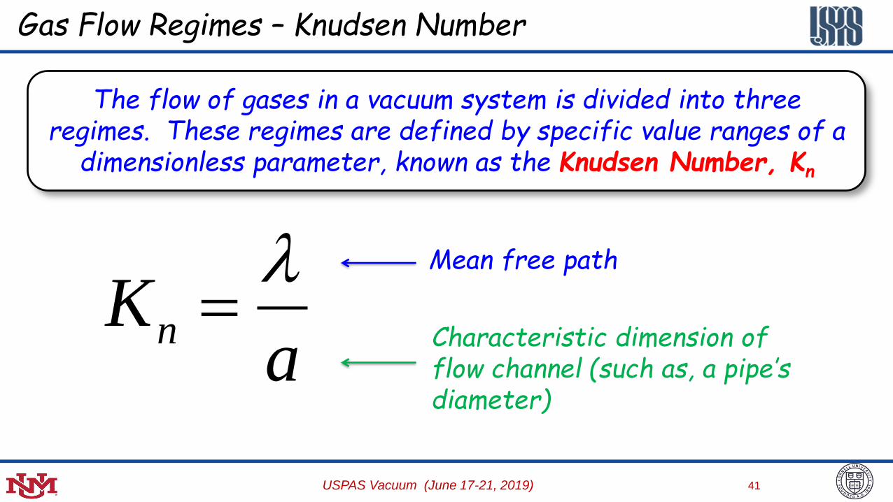
The flow of gases in a vacuum system is divided into three regimes. These regimes are defined by specific value ranges of a
dimensionless parameter, known as the Knudsen Number, Kn
Gas Flow Regimes – Knudsen Number
aKn
Mean free path
Characteristic dimension of flow channel (such as, a pipe’s diameter)
USPAS Vacuum (June 17-21, 2019)

42
Three Gas Flow Regimes
Transition Flow: 0.101.0 nK
Viscous Flow:
01.0a
Kn
Characterized by molecule-molecule collisions
Molecular Flow:
0.1nKCharacterized by molecule-wall collisions
Press
ure
USPAS Vacuum (June 17-21, 2019)

43
Viscous (or Continuum) Flow
The character of the flow is determined by gas-gas collisions
Molecules travel in uniform motion toward lower pressure, molecular motion ‘against’ flow direction unlikely
The flow can be either turbulent or laminar, characterized by another dimensionless number, the Reynolds’ number, R
USPAS Vacuum (June 17-21, 2019)

44
Viscous Flow – Reynolds’ Number
dURe
U – stream velocity – gas densityd – pipe diameter – viscosity
Laminar Flow: zero flow velocity at wall
R < 1200 Turbulent Flow: eddies at wall and strong mixing
R > 2100
Reynolds’ Number, Re is the ratio of inertia vs. viscosity
USPAS Vacuum (June 17-21, 2019)

45
Throughput
Throughput is defined as the quantity of gas flow rate, that is, the volume of gas at a known pressure passing a plane in a known time
dt
PVdQ
)(
In SI unit, [Q] = Pa-m3/s ( = 7.5 torr-liter/s)
Interesting Point: Pa-m3/s = N-m/s = J/s = Watt !
USPAS Vacuum (June 17-21, 2019)

P2 P1
P2 > P1
Q
46
Gas Conductance – Definition
The flow of gas (throughput) in a duct or pipe depends on the pressure differential, as well on the connection geometry
The gas conductance of the connection is defined:
12 PP
QC
In SI unit: m3/s
Commonly used: liter/s
USPAS Vacuum (June 17-21, 2019)

47
Vacuum Pump – Pumping Speed
Defined as a measure of volumetric displacement rate, (m3/sec, cu-ft/min, liter/sec, etc.)
The throughput of a vacuum pump is related the pressure at the pump inlet as:
dtdVS
SPdt
dVPQ
USPAS Vacuum (June 17-21, 2019)

USPAS Vacuum (June 17-21 2019) 48
Typical Gas Conductance vs. Pressure
• Independent of pressure in the molecular flow regime
• proportional to the mean pressure in the viscous flow regime
• Knudsen flow represents a transition between the two types of flow, and the conductivities vary with the Knudsen number

49
Gas Conductance – Continuum Flow
Viscous flow is usually encountered during vacuum system roughing down processes.
Gas flow in the viscous flow regime is very complicated. A great amount of theoretic works can be found in the literatures on the subject.
Direct simulation Monte Carlo (DSMC) codes are widely used to calculate the flow in the region.
Depending the value of Reynolds’ number, the flow can be either laminar or turbulent.
Turbulent flow is usually to be avoided (by ‘throttling’), to reduce contamination (to the upstream system), and to reduce vibration.
USPAS Vacuum (June 17-21, 2019)

50
Gas Conductance – Continuum Flow (2)
The gas throughput (and conductance) is dependent on both the ‘inlet’ pressure and the ‘outlet’ pressure in most situations, and (of course) on the piping geometry.
The flow usually increases with reduced outlet pressure, but may be “choked’ when the gas stream speed exceeding the speed of sound.
Flow through a thin orifice
1.00.50.0
Poutlet/Pinlet
Q / A
USPAS Vacuum (June 17-21, 2019)
𝑄𝑐ℎ𝑜𝑘𝑒𝑑 = 15.7 ∙ 𝑑(𝑐𝑚)2 ∙ 𝑃𝐼𝑛𝑙𝑒𝑡(𝑚𝑏𝑎𝑟)
For Air

51
Molecular Flow – Orifices
n1
P1
n2
P2
If two large vessels are connected by an thin orifice of opening area A, then gas flow from vessel 1 to vessel 2 is given by the particle flux exchange:
)(4
)(4
2121 PPAv
nnvAkT
Q
From definition of the conductance:
Av
PP
QC
421
USPAS Vacuum (June 17-21, 2019)

52
Molecular Flow – Orifices (2)
mkTv
8 )(24.36)/( 23 mAM
TsmC
amu
Orifice
where: T is temperature in Kevin; Mamu is molecular mass in atomic mass unit
For air (Mamu=28.97) at 22C:
C (m3/s) = 116 A (m2)
Or: C (L/s) = 11.6 A (cm2)
USPAS Vacuum (June 17-21, 2019)

53
Molecular Flow – Long Round Tube
l
d
M
T
l
dvC
amu
33
94.3712
where T is the temperature in Kevin, M the molecular mass in AMU, d and l
are diameter and length of the tube in meter, with l >> d
For air (Mamu=28.97) at 22C:
l
dsmC
33 121)/(
From Knudson (1909)
USPAS Vacuum (June 17-21, 2019)

54
Molecular Flow – Short Tube
No analytical formula for the short pipe conductance. But for a pipe of constant cross section, it is common to introduce a parameter called transmission
probability, a, so that:
Av
CC Orifice4
aa
where A is the area of the pipe cross section.
For long round tube, the transmission probability is:
ld
tubelong 34
_ a
USPAS Vacuum (June 17-21, 2019)

55
Molecular Flow – Transmission of Round Tube
l/d a l/d a l/d a
1.000000.00
0.952400.05
0.909220.10
0.869930.15
0.834080.20
0.801270.25
0.771150.30
0.743410.35
0.717790.40
0.694040.45
0.691780.50
0.651430.55
0.632230.60
0.597370.70
0.566550.80
0.538980.9
0.514231.0
0.491851.1
0.471491.2
0.452891.3
0.435811.4
0.420061.5
0.405481.6
0.379351.8
0.356582.0
0.310542.5
0.275463.0
0.247763.5
0.225304.0
0.206694.5
0.190995.0
0.165966.0
0.146847.0
0.131758.0
0.119519.0
0.1093810
0.0769915
0.0594920
0.0485125
0.0409730
0.0354635
0.0312740
0.0252950
2.65x10-2500
5000 2.66x10⁻³
USPAS Vacuum (June 17-21, 2019)
𝛼 =𝐴1
𝐴1 + ൗ𝑙 𝑑
𝐴2
with
A1 = 1.0667
A2 = 0.94629

56
Molecular Flow – Transmission of Round Tube
Long tube formula valid when l/d > 10
1.5
1.0
0.5
0.0
-0.5
-1.0
Fit R
esidu
al (%
)
0.1 1 10
0.0001
0.001
0.01
0.1
1
Tran
smis
sion
Pro
babi
lity
10-2
10-1
100
101
102
103
104
l/d
Fit function (l/d< 50)
2
1
1
A
dlA
A
dlT
Long Tube Transmission 4d/3l
USPAS Vacuum (June 17-21, 2019)

57
Gas Conductance of Rectangular Ducts
REF. D.J. Santeler and M.D. Boeckmann, J. Vac. Sci. Technol. A9 (4) p.2378, 1991
0,, ClcbC rect a
C0 is the entrance aperture conductance;
arect(b,c,l) is the transmission probability,
depending on geometry and length
of the duct
2/1
0 64.3 MTbcC
C0 in liter/sec; b, c are height and width of the duct in cm
T is gas temperature in Kevin; M is the molar mass of the gas
USPAS Vacuum (June 17-21, 2019)

58
Transmission of Long Rectangular Ducts
For a very long rectangular duct, the transmission probability can be calculated by the modified Knudson equation:
KRRLcbl
bcKvl
8/13
1
3
8
a
where L and R are defined as:
blL bc
bcR
and K is a correcting factor reflecting geometrical shape of the duct
R 1.0 1.5 2.0 3.0 4.0 6.0 8.0 12.0 16.0 24.0
K(R) 1.115 1.127 1.149 1.199 1.247 1.330 1.398 1.505 1.588 1.713
REF. D.J. Santeler and M.D. Boeckmann, J. Vac. Sci. Technol. A9 (4) p.2378, 1991
USPAS Vacuum (June 17-21, 2019)

59
Transmission of Rectangular Ducts
RRLs
2/11
1
a
Short rectangular duct
RKRLl
8/131
1
a
(Medium) Long rectangular duct
l
E
s
E
RLD
RLD
aaa
1
/1
Rectangular duct of any length – empirical equation
where D and E are fitting parameters
USPAS Vacuum (June 17-21, 2019)

60
Transmission of Rectangular Ducts – Computed
R=c/b 1 1.5 2 3 4 6 8 12 16 24
D 0.8341 0.9446 1.0226 1.1472 1.2597 1.4725 1.6850 2.1012 2.5185 3.3624
E 0.7063 0.7126 0.7287 0.7633 0.7929 0.8361 0.8687 0.9136 0.9438 0.9841
Fitted parameters for transmission equation
REF. D.J. Santeler and M.D. Boeckmann, J. Vac. Sci. Technol. A9 (4) p.2378, 1991
USPAS Vacuum (June 17-21, 2019)

61
Transmission of Rectangular Ducts – Cont.
Comparing numerically computed transmission with as, al and corrected a.
USPAS Vacuum (June 17-21, 2019)

62
Transmission of Rectangular Ducts – Parameters
Fit K D E
A01.0663 0.7749 0.6837
A10.0471 0.1163 0.02705
A2- 8.48x10⁻⁴ - 3.72x10⁻⁴ - 6.16x10⁻⁴
3rd-order polynomial fits are used for any rectangular cross sections (c/b as variable):
2,,
2
,,
1
,,
0,, RARAAEDK EDKEDKEDK 3.5
3.0
2.5
2.0
1.5
1.0
0.5
Par
amet
ers
for C
alcu
latin
g R
ect P
ipe
Tran
smis
sion
2520151050
Pipe Width / Height
D & fit E & fit K & fit
bcb
cR
USPAS Vacuum (June 17-21, 2019)
63
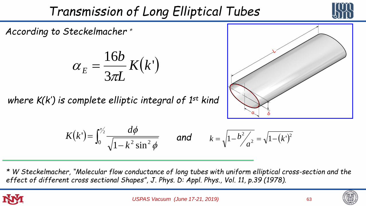
Transmission of Long Elliptical Tubes
'3
16kK
L
bE
a
where K(k’) is complete elliptic integral of 1st kind
According to Steckelmacher
22
2
'11 ka
bk
2
0 22 sin1'
k
dkK and
* W Steckelmacher, “Molecular flow conductance of long tubes with uniform elliptical cross-section and the effect of different cross sectional Shapes”, J. Phys. D: Appl. Phys., Vol. 11, p.39 (1978).
USPAS Vacuum (June 17-21, 2019)

64
Calculating Elliptic Integral
The elliptic integral has to be calculated numerically, but here is a web calculator for the complete elliptic integral of 1st kind.
6
5
4
3
2
1
Com
plet
e E
llipt
ic I
nteg
ral K
7 8 9
0.012 3 4 5 6 7 8 9
0.12 3 4 5 6 7 8 9
1
k' = b/a
Elliptic Integral Definition :
Fit to :
USPAS Vacuum (June 17-21, 2019)
65
Transmission of Short Elliptical Tubes
1.0
0.8
0.6
0.4
0.2
0.0
Elli
ptic
al T
ube
Tra
nsm
issi
on
1086420
Normalized Tube Length (L/b)
a/b = 10 a/b = 5 a/b = 3 a/b = 2 a/b = 1
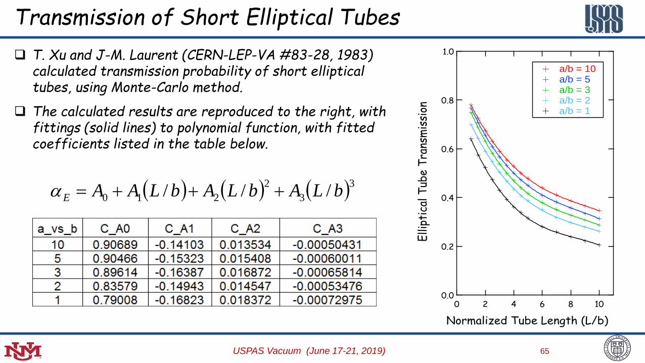
T. Xu and J-M. Laurent (CERN-LEP-VA #83-28, 1983) calculated transmission probability of short elliptical tubes, using Monte-Carlo method.
The calculated results are reproduced to the right, with fittings (solid lines) to polynomial function, with fitted coefficients listed in the table below.
33
2
210 /// bLAbLAbLAAE a
USPAS Vacuum (June 17-21, 2019)
66
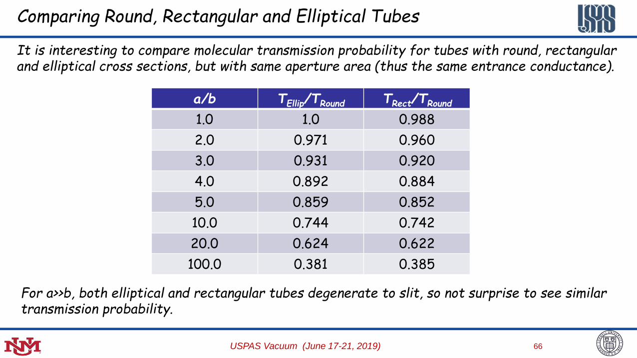
Comparing Round, Rectangular and Elliptical Tubes
It is interesting to compare molecular transmission probability for tubes with round, rectangular and elliptical cross sections, but with same aperture area (thus the same entrance conductance).
a/b TEllip/TRound TRect/TRound
1.0 1.0 0.988
2.0 0.971 0.960
3.0 0.931 0.920
4.0 0.892 0.884
5.0 0.859 0.852
10.0 0.744 0.742
20.0 0.624 0.622
100.0 0.381 0.385
For a>>b, both elliptical and rectangular tubes degenerate to slit, so not surprise to see similar transmission probability.
USPAS Vacuum (June 17-21, 2019)

67
Monte Carlo Test Particle Calculations
Monte Carlo (MC) statistic method is often used to calculate complex, but practical vacuum components, such as elbows, baffles, traps, etc.
In MC calculations, a large number of test particles are ‘injected’ at entrance, and tracked through the geometry.
One of such MC packages, MolFlow+ is available through the authors.
USPAS Vacuum (June 17-21, 2019)

68
Transmission Calculations Using MolFlow+
Ø1cm, 10 cm long
straight tube
Ø1cm, 10 cm long elbow
Ø1cm, 10 cm long
U-tube
Straight a = 0.109
90 Elbow a = 0.105
180 U a = 0.093
These simple calculations took <1-minute
USPAS Vacuum (June 17-21, 2019)

69
Combining Molecular Conductances
The conductance of tubes connected in parallel can be obtained from simple sum, and is independent of any end effects.
CT = C1 + C2 + C3 +, …, + Cn
Series conductances of truly independent elements can be calculated:
NT CCCC
1...
111
21
The series elements must be separated by large volumes, so that
the molecular flow is re-randomized before entering next element
C1
C2
USPAS Vacuum (June 17-21, 2019)