Validated Solutions of Initial Value Problems for Parametric ODEs

Youdong Lin and Mark A. Stadtherr∗

Department of Chemical and Biomolecular EngineeringUniversity of Notre Dame, Notre Dame, IN 46556, USA

(revised, October 2006)Accepted for publication in Applied Numerical Mathematics

Abstract

In initial value problems for ODEs with interval-valued parameters and/or initial values, itis desirable in many applications to be able to determine a validated enclosure of all possiblesolutions to the ODE system. Much work has been done for the case in which initial values aregiven by intervals, and there are available software packages that deal with this case. However,less work has been done on the case in which parameters are given by intervals. We describehere a new method for obtaining validated solutions of initial value problems for ODEs withinterval-valued parameters. The method also accounts for interval-valued initial values. The ef-fectiveness of the method is demonstrated using several numerical examples involving parametricuncertainties.

Keywords: Ordinary differential equations; Interval analysis; Validated computing; Taylormodels; Dynamic systems

1 Introduction

Initial value problems (IVPs) for ordinary differential equations (ODEs) arise naturally in manyapplications in science and engineering. It is often the case that the problem involves parametersand/or initial values that are not known with certainty but that can be expressed as intervals.For this situation it is desirable to be able to determine an enclosure of all possible solutions tothe ODEs. Traditional approximate solution methods for ODEs are not useful in this context,since, in essence, they would have to solve infinitely many systems to determine such an enclosure.Interval methods [25] for ODEs, on the other hand, provide a natural approach for computing thedesired enclosure. Even in the case in which the initial values and parameters are known exactly,standard numerical methods for solving ODEs only compute an approximate solution to sometolerance, without guaranteed error bounds, and so it is of interest to determine an enclosure of thetrue solution. Interval methods (also called validated methods or verified methods) not only candetermine a guaranteed error bound on the true solution, but can also verify that a unique solutionto the problem exists. An excellent review of interval methods for IVPs has been given by Nedialkov

∗Author to whom all correspondence should be addressed. Phone: (574) 631-9318; Fax: (574) 631-8366; E-mail:markst@nd.edu

1

et al. [28]. Much work has been done for the case in which the initial values are given by intervals,and there are several available software packages that deal with this case. However, relativelylittle work has apparently been done on the case in which parameters are given by intervals. Weconcentrate here on the case of such parametric ODEs. However, the method developed will alsoaccount for interval-valued initial values.

Traditional interval methods usually consist of two processes applied at each integration step[28]. In the first process, existence and uniqueness of the solution are proven, and a rough en-closure of the solution is computed. In the second process, a tighter enclosure of the solution iscomputed. This can be regarded as similar to the familiar predictor-corrector procedure employedin many standard methods for obtaining an approximate solution. In general, both processes arerealized by applying interval Taylor series (ITS) expansions with respect to time, and using au-tomatic differentiation to obtain the Taylor coefficients. A major difficulty in interval methodsis the overestimation of bounds caused by the dependency problem of interval arithmetic and bythe wrapping effect [25]. The accumulation of overestimations at successive time steps may ulti-mately lead to an explosion of enclosure sizes, causing the integration procedure to abort. Severalschemes for reducing the overestimation of bounds have been proposed. For example, Lohner’sAWA package employs a QR-factorization method which features efficient coordinate transforma-tions to tackle the wrapping effect [15]. Nedialkov’s VNODE package employs QR together with aninterval Hermite-Obreschkoff method [27, 29], which can be viewed as a type of generalized Taylormethod, and improves on AWA. Janssen et al. [7] have introduced a constraint satisfaction ap-proach to these problems, which enhances traditional interval methods with a pruning step basedon a global relaxation of the ODEs. Another approach for addressing the dependency problemand the wrapping effect has been described by Berz and Makino [3] and implemented in the beamdynamics package COSY INFINITY. This scheme is based on expressing the dependence on initialvalues and time using a Taylor model (i.e., a Taylor polynomial and an interval remainder bound).Neher et al. [30] have recently described this Taylor model approach in some detail and comparedit to traditional interval methods. We will also use Taylor models in the new method describedhere, though they will be determined and used in a different way, and a new type of Taylor modelwill be introduced.

Available general-purpose validated ODE solvers are focused on dealing with uncertainties inthe initial values. Some solvers, including VNODE [26], can take interval parameters as input.These solvers, however, can become very inefficient in the presence of interval parameters becausethis tends to exacerbate the wrapping effect; thus the size of the enclosure can grow so quicklythat the integration must be stopped. An alternative approach is to treat time-invariant intervalparameters as additional state variables, with zero first-order derivatives, as suggested by Lohner[16]. Since the parameters are now treated as independent variables, tighter enclosures can beobtained using this approach. However, the increase in the number of state variables can result ina significant increase in the computational expense. For example, in a problem with n states andp parameters, an (n + p) × (n + p) matrix, instead of an n × n matrix, must be factored at eachtime step in the usual approach for controlling the wrapping effect. In the work described here,we will develop a method for efficiently determining validated solutions of ODEs with parametricuncertainties, where instead of increasing the number of state variables, we will treat the parametricuncertainties directly. The method follows the traditional two-phase interval approach, but makesuse, in a novel way, of Taylor models.

Singer and Barton [35] have recently suggested another approach for bounding the solutions ofparametric ODEs. They use convex underestimators and concave overestimators to construct two

2

bounding IVPs, which are then solved to obtain the lower and upper bounds on the trajectories.However, as implemented [34], the bounding IVPs are solved using standard numerical methods thatdo not provide guaranteed error estimates. Thus, this approach cannot be regarded as providingrigorously guaranteed enclosures.

The remainder of this paper is organized as follows. Section 2 describes the problem we areaddressing and the notation used. Section 3 provides background on interval analysis and a briefintroduction to the use of Taylor models, based on the Taylor model arithmetic (remainder differ-ential algebra) described by Makino and Berz [20, 23]. Section 4 presents the new interval methodfor obtaining guaranteed enclosures of the solutions of parametric ODEs. Then, in Section 5 wepresent the results of several numerical experiments that demonstrate the effectiveness of the newmethod.

2 Problem Description

In this section we describe the problem to be solved, and introduce our notation. We considervalidated numerical methods for solving the set of parametric autonomous IVPs

y′(t) = f(y, θ), y(t0) = y0 ∈ Y0, θ ∈ Θ, (1)

where t ∈ [t0, tm] for some tm > t0. Here θ is a p-dimensional vector of time-invariant parameters,y is the n-dimensional vector of state variables, and y0 is the n-dimensional vector of initial values.The interval vectors Θ and Y0 represent enclosures of the uncertainties in θ and y0, respectively.Uppercase will be used to denote interval-valued quantities, unless noted otherwise. We assumethat f : R

n × Rp → R

n is (k − 1)-times continuously differentiable with respect to the statevariables y on R

n, and (q + 1)-times continuously differentiable with respect to the parametersθ on R

p. Here, k is the order of the truncation error in the ITS method to be used, and q isthe order of the Taylor model to be used to represent dependence on the uncertain quantities(parameters and/or initial values). We also assume that the representation of f contains a finitenumber of constants, variables, elementary operations, and standard functions. Because of thedifferentiability requirement, functions such as branches, abs, min or max are excluded.

A sequence of values, t0 < t1 < · · · < tm will be considered, with step size hj = tj+1 − tj (notnecessarily constant) at the (j+1)-th integration step, j = 0, . . . ,m−1. A solution of y ′(t) = f(y, θ)for the initial condition y = yj at t = tj is denoted by y(t; tj , yj , θ). We denote by y(t; tj, Yj ,Θ) theset of solutions

y(t; tj , Yj ,Θ) = {y(t; tj , yj, θ) | yj ∈ Yj, θ ∈ Θ} . (2)

In this work, we seek to determine enclosures Yj, j = 1, . . . ,m, of the state variables at each timestep such that

y(tj ; t0, Y0,Θ) ⊆ Yj , (3)

and to do so in such a way that there will be relatively little overestimation.

Traditional interval methods for solving (1) involve the use of Taylor series expansions withrespect to time. In a Taylor expansion of y(t) with respect to time, the i-th Taylor coefficientevaluated at tj is denoted by

(yj)i =y(i)(tj)

i!, (4)

3

where y(i)(t) is the i-th derivative of y(t). In terms of f(y, θ) = y ′(t), these Taylor coefficients canbe expressed recursively using functions denoted by f [i] as

(yj)0 = f [0](yj, θ) = yj (5)

(yj)1 = f [1](yj, θ) = f(yj, θ) (6)

(yj)i = f [i](yj , θ) =1

i

(∂f [i−1]

∂yf

)(yj, θ), i ≥ 2. (7)

This allows for the efficient generation of Taylor coefficients [25]. Interval extensions, (Yj)i =F [i](Yj ,Θ), of the Taylor coefficients for yj ∈ Yj and θ ∈ Θ can be generated by using the sameprocedure in interval arithmetic, as discussed in the next section, or by using other methods, asdescribed in Section 4.

3 Background

3.1 Interval analysis

A real interval C is defined as the set of real numbers lying between (and including) given upperand lower bounds; that is,

C =[C,C

]={c ∈ R | C ≤ c ≤ C

}. (8)

Here an underline is used to indicate the lower bound of an interval and an overline is used to indicatethe upper bound. Thus, uppercase quantities with underline or overline are real. The set of allreal intervals is denoted by IR. For an interval C = [C,C], the width is denoted by w(C) = C − Cand the midpoint by m(C) = (C + C)/2. A real interval vector X = (X1, X2, · · · , Xn)T ∈ IR

n hasn real interval components and can be interpreted geometrically as an n-dimensional rectangle orbox. Interval matrices can be similarly defined. For an interval vector or matrix, the width andmidpoint are defined componentwise.

Basic arithmetic operations with intervals are defined by

X op Y = {x op y | x ∈ X, y ∈ Y } , (9)

where op = {+,−,×,÷}. Interval versions of the elementary functions can be similarly defined.It should be emphasized that, when machine computations with interval arithmetic operationsare done, as in the procedures outlined below, the endpoints of an interval are computed with adirected (outward) rounding. That is, the lower endpoint is rounded down to the next machine-representable number and the upper endpoint is rounded up to the next machine-representablenumber. In this way, through the use of interval, as opposed to floating-point arithmetic, anypotential rounding error problems are avoided. Several good introductions to interval analysis, aswell as interval arithmetic and other aspects of computing with intervals, are available [8, 6, 9, 31].Implementations of interval arithmetic and elementary functions are also readily available, andrecent compilers from Sun Microsystems directly support interval arithmetic and an interval datatype.

For an arbitrary function g(x), the interval extension, denoted by G(X), encloses all possiblevalues of g(x) for x ∈ X. That is, G(X) ⊇ {g(x) | x ∈ X} encloses the range of g(x) over X. It is

4

often computed by substituting the given interval X into the function g(x) and then evaluating thefunction using interval arithmetic. This “natural” interval extension may be wider than the actualrange of function values, although it always includes the actual range. For example, the naturalinterval extension of g(x) = x/(x − 1) over the interval X = [2, 3] is G([2, 3]) = [2, 3]/([2, 3] − 1) =[2, 3]/[1, 2] = [1, 3], while the true function range over this interval is [1.5, 2]. This overestimation ofthe function range is due to the “dependency” problem of interval arithmetic, which may arise whena variable occurs more than once in a function expression. While a variable may take on any valuewithin its interval, it must take on the same value each time it occurs in an expression. However,this type of dependency is not recognized when the natural interval extension is computed. Ineffect, when the natural interval extension is used, the range computed for the function is the rangethat would occur if each instance of a particular variable were allowed to take on a different valuein its interval range. For the case in which g(x) is a single-use expression, that is, an expression inwhich each variable occurs only once, natural interval arithmetic will always yield the true functionrange. For example, rearrangement of the function expression used above gives g(x) = x/(x− 1) =1 + 1/(x − 1), and now G([2, 3]) = 1 + 1/([2, 3] − 1) = 1 + 1/[1, 2] = 1 + [0.5, 1] = [1.5, 2], the truerange. There are a variety of approaches that can be used to try to avoid the overestimation thatmay occur due to the dependency problem, including the use of Taylor models, as described in thenext subsection.

3.2 Taylor models

Makino and Berz [20] have described a remainder differential algebra (RDA) approach forbounding function ranges and control of the dependency problem of interval arithmetic [21]. Inthis method a function is represented using a model consisting of a Taylor polynomial and aninterval remainder bound.

One way of forming a Taylor model of a function is by using a truncated Taylor series. Considera function f : x ∈ X ⊂ R

m → R that is (q + 1) times partially differentiable on each componentof x, and let x0 ∈ X. The Taylor theorem states that for each x ∈ X, there exists a ζ ∈ R with0 < ζ < 1 such that

f(x) =

q∑

i=0

1

i![(x − x0) · 5]i f (x0) +

1

(q + 1)![(x − x0) · 5]q+1 f [x0 + (x − x0)ζ] , (10)

where the partial differential operator [g · 5]k is

[g · 5]k =∑

j1+···+jm=k

0≤j1 ,··· ,jm≤k

k!

j1! · · · jm!gj11 · · · gjm

m

∂k

∂xj11 · · · ∂xjm

m

. (11)

The last (remainder) term in (10) can be quantitatively bounded over 0 < ζ < 1 using intervalarithmetic or other methods to obtain an interval remainder bound Rf . The summation in (10) isa q-th order polynomial (truncated Taylor series) in (x − x0) which we denote by pf (x − x0). Aq-th order Taylor model Tf = pf + Rf for f(x) then consists of the polynomial pf and the intervalremainder bound Rf and is denoted by Tf = (pf , Rf ). Note that f ∈ Tf for x ∈ X and thus Tf

encloses the range of f over X.

Taylor models of functions can also be formed by performing Taylor model operations. Arith-metic operations with Taylor models can be done using the remainder differential algebra (RDA)

5

described by Makino and Berz [20, 23]. Let Tf and Tg be the Taylor models of the functions f(x)and g(x), respectively, over the interval x ∈ X. For f ± g,

f ± g ∈ Tf ± Tg = (pf , Rf ) ± (pg, Rg) = (pf ± pg, Rf ± Rg). (12)

Thus a Taylor model of f ± g is given by

Tf±g = (pf±g, Rf±g) = (pf ± pg, Rf ± Rg). (13)

For the product f × g,

f × g ∈ (pf , Rf ) × (pg, Rg) ⊆ pf × pg + pf × Rg + pg × Rf + Rf × Rg. (14)

Note that pf × pg is a polynomial of order 2q. Since a q-th order polynomial is sought for theTaylor model of f × g, this term is split pf × pg = pf×g + pe. Here the polynomial pf×g containsall terms of order q or less, and pe contains the higher order terms. A q-th order Taylor model forthe product f × g can then be given by Tf×g = (pf×g, Rf×g), with

Rf×g = B(pe) + B(pf ) × Rg + B(pg) × Rf + Rf × Rg. (15)

Here B(p) = P (X − x0) denotes an interval bound on the polynomial p(x − x0) over x ∈ X.Similarly, an interval bound on an overall Taylor model T = (p,R) will be denoted by B(T ), and iscomputed by obtaining B(p) and adding it to the remainder bound R; that is, B(T ) = B(p) + R.The method we use to obtain the polynomial bounds is described below. In storing and operatingon a Taylor model, only the coefficients of the polynomial part p are used, and these are pointvalued. However, when these coefficients are computed in floating point arithmetic, numericalerrors may occur and they must be bounded. To do this in our current implementation of Taylormodel arithmetic, we have used the “tallying variable” approach, as described by Makino and Berz[23]. This approach has been analyzed in detail by Revol et al. [33]. This results in an error boundon the floating point calculation of the coefficients in p being added to the interval remainder boundR.

Taylor models for the reciprocal operation, as well as the intrinsic functions (exponential, loga-rithm, square root, sine, cosine, etc.) can also be obtained [19, 20, 23]. Using these, together withthe basic arithmetic operations defined above, it is possible to start with simple functions such asthe constant function f(x) = k, for which Tf = (k, [0, 0]), and the identity function f(xi) = xi,for which Tf = (xi0 + (xi − xi0), [0, 0]), and then to compute Taylor models for very complicatedfunctions. Altogether, it is possible to compute a Taylor model for any function that can be rep-resented in a computer environment by simple operator overloading through RDA operations. Ithas been shown that, compared to other rigorous bounding methods, the Taylor model often yieldssharper bounds for modest to complicated functional dependencies [20, 21, 32]. A discussion of theuses and limitations of Taylor models has been given by Neumaier [32].

The range bounding of the interval polynomials B(p) = P (X −x0) is an important issue, whichdirectly affects the performance of Taylor model methods. Unfortunately, exact range bounding ofan interval polynomial is NP hard, and direct evaluation using interval arithmetic is very inefficient,often yielding only loose bounds. Thus, various bounding schemes [24, 32] have been used, mostlyfocused on exact bounding of the dominant parts of P , i.e., the first- and second-order terms.However, exact bounding of a general interval quadratic is also computationally expensive (inthe worst case, exponential in the number of variables m). Thus, we have adopted here a very

6

simple compromise approach, in which only the first-order and the diagonal second-order terms areconsidered for exact bounding, and other terms are evaluated directly. That is,

B(p) =

m∑

i=1

[ai (Xi − xi0)

2 + bi(Xi − xi0)]

+ Q, (16)

where Q is the interval bound of all other terms, and is obtained by direct evaluation with intervalarithmetic. In (16), since Xi occurs twice, there exists a dependency problem. For |ai| ≥ ω, whereω is a small positive number, we can rearrange Eq. 16 such that each Xi occurs only once; that is,

B(p) =

m∑

i=1

[ai

(Xi − xi0 +

bi

2ai

)2

−b2i

4ai

]+ Q. (17)

In this way, the dependence problem in bounding the interval polynomial is alleviated so that asharper bound can be obtained. If |ai| < ω, direct evaluation will be used instead.

4 Validated Parametric ODE Solver

In traditional interval Taylor series (ITS) methods for IVPs for ODEs, each integration stepconsists of two phases: 1. Validating existence and uniqueness; 2. Computing a tighter enclosure.The traditional methods are focused on handling interval-valued uncertainties in the initial con-ditions, and do not explicitly account for dependence on a parameter vector. Thus, in problemswith interval-valued parameters, the interval dependency problem can quickly cause the size of theenclosure to become unacceptable, perhaps leading to premature termination of the integrationprocess. As noted above, by treating interval parameters as additional state variables [16], tighterenclosures may be obtained using traditional methods. However, the increase in the number of statevariables can result in a significant increase in the computational expense, due to, for example, thematrix factorizations used to control wrapping. In this section, we present a new method for thevalidated solution of the parametric ODE system defined by (1). A two-phase approach is used inwhich the dependence of y′(t) = f(y, θ) on t is handled using ITS methods. However, in the enclo-sure tightening phase, the dependence on the parameter vector θ is handled using Taylor models interms of the parameters. Interval-valued uncertainties in the initial conditions are handled in thesame way. This allows for efficient control of the interval dependency problem, and also leads to anew method for dealing with the wrapping effect. The technique for addressing the wrapping effectis based on a new type of Taylor model in which the enclosure of the remainder is an n-dimensionalparallelepiped, rather than an interval.

4.1 Validating existence and uniqueness

In phase 1, we apply the traditional method to the parametric ODEs by using an intervalTaylor series with respect to time. The approach used is essentially the same as in the traditionalmethod, except that parameter dependence is explicitly accounted for. Assume that at tj we havean enclosure Yj of y(tj; t0, Y0,Θ). The goal is to find a step size hj = tj+1 − tj > 0 and an a priori

enclosure (coarse enclosure) Yj of the solution such that a unique solution y(t) is guaranteed to

exist for all t ∈ [tj , tj+1], all yj ∈ Yj , all θ ∈ Θ, and y(t; tj , Yj,Θ) ⊆ Yj.

7

Using the Picard-Lindelof operator and the Banach fixed-point theorem [5], it can be shownthat if hj and Yj ⊆ Y 0

j satisfy

Yj = Yj + [0, hj ]F (Y 0j ,Θ) ⊆ Y 0

j , (18)

then there is a unique solution y(t; tj , yj , θ) that satisfies y(t; tj , yj , θ) ∈ Yj for all t ∈ [tj , tj+1], allyj ∈ Yj , all θ ∈ Θ. The method based on (18) is referred as a first-order (or constant) enclosuremethod. While an hj for which (18) can be satisfied can always be found, this step size may bevery small. Thus, high-order enclosure methods are commonly used that can enable larger stepsizes by using polynomial enclosures [17] or more Taylor series terms [25, 28] in the sum in (18).Following the latter method, we determine hj and Yj such that

Yj =

k−1∑

i=0

[0, hj ]iF [i](Yj,Θ) + [0, hj ]

kF [k](Y 0j ,Θ) ⊆ Y 0

j . (19)

Following the approach of Corliss and Rihm [4, Theorem 3], it can be shown that if (19) is satisfied,then there exists a unique solution y(t; tj, yj , θ) ∈ Yj for all t ∈ [tj, tj+1], all θ ∈ Θ and all yj ∈ Yj .The approach used to implement phase 1 is similar to that used in VNODE [26].

4.2 Computing a tighter enclosure

In phase 2, we compute a tighter enclosure Yj+1 ⊆ Yj such that y(tj+1; t0, Y0,Θ) ⊆ Yj+1. Thiswill be done by using an ITS approach to compute a Taylor model Tyj+1 of yj+1 in terms of theparameters and initial values, and then obtaining the enclosure Yj+1 from Yj+1 = B(Tyj+1).

For the Taylor model computations, we begin by representing the interval initial values y0 ∈ Y0

by the Taylor model Ty0 , with components

Ty0i= (m(Y0i) + (y0i − m(Y0i)), [0, 0]), i = 1, · · · , n. (20)

The interval parameters are represented by the Taylor model Tθ, with components

Tθi= (m(Θi) + (θi − m(Θi)), [0, 0]), i = 1, · · · , p. (21)

We can now determine Taylor models Tf [i] of the ITS coefficients f [i](yj, θ) by using RDA operations

and (7) to compute Tf [i] = f [i](Tyj, Tθ). The polynomial part of Tf [i] is specified to be of order q, and

is a function of the parameters θ and initial values y0 (p+n total variables). Thus, Tf [i] = Tf [i](y0, θ).

Now consider the interval Taylor series with respect to time

yj+1 = yj +k−1∑

i=1

hijf

[i](yj , θ) + hkj f

[k](y; tj , tj+1, θ), (22)

where yj ∈ Yj, and f [k](y; tj , tj+1, θ) denotes f [k] with its l-th component (l = 1, . . . , n) evaluated

at y(ξj,l) for some ξj,l ∈ [tj , tj+1], which can be enclosed by F [k](Yj ,Θ). To get an enclosureYj+1 from (22), enclosures of the ITS coefficients f [i](yj , θ), i = 1, . . . , k − 1 are needed. Onetraditional approach for doing this is to evaluate these coefficients in interval arithmetic, that is

8

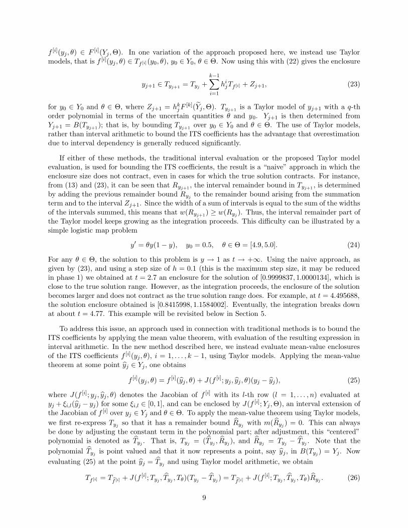
f [i](yj, θ) ∈ F [i](Yj ,Θ). In one variation of the approach proposed here, we instead use Taylormodels, that is f [i](yj , θ) ∈ Tf [i](y0, θ), y0 ∈ Y0, θ ∈ Θ. Now using this with (22) gives the enclosure

yj+1 ∈ Tyj+1 = Tyj+

k−1∑

i=1

hijTf [i] + Zj+1, (23)

for y0 ∈ Y0 and θ ∈ Θ, where Zj+1 = hkj F

[k](Yj ,Θ). Tyj+1 is a Taylor model of yj+1 with a q-thorder polynomial in terms of the uncertain quantities θ and y0. Yj+1 is then determined fromYj+1 = B(Tyj+1); that is, by bounding Tyj+1 over y0 ∈ Y0 and θ ∈ Θ. The use of Taylor models,rather than interval arithmetic to bound the ITS coefficients has the advantage that overestimationdue to interval dependency is generally reduced significantly.

If either of these methods, the traditional interval evaluation or the proposed Taylor modelevaluation, is used for bounding the ITS coefficients, the result is a “naive” approach in which theenclosure size does not contract, even in cases for which the true solution contracts. For instance,from (13) and (23), it can be seen that Ryj+1 , the interval remainder bound in Tyj+1 , is determinedby adding the previous remainder bound Ryj

to the remainder bound arising from the summationterm and to the interval Zj+1. Since the width of a sum of intervals is equal to the sum of the widthsof the intervals summed, this means that w(Ryj+1) ≥ w(Ryj

). Thus, the interval remainder part ofthe Taylor model keeps growing as the integration proceeds. This difficulty can be illustrated by asimple logistic map problem

y′ = θy(1 − y), y0 = 0.5, θ ∈ Θ = [4.9, 5.0]. (24)

For any θ ∈ Θ, the solution to this problem is y → 1 as t → +∞. Using the naive approach, asgiven by (23), and using a step size of h = 0.1 (this is the maximum step size, it may be reducedin phase 1) we obtained at t = 2.7 an enclosure for the solution of [0.9999837, 1.0000134], which isclose to the true solution range. However, as the integration proceeds, the enclosure of the solutionbecomes larger and does not contract as the true solution range does. For example, at t = 4.495688,the solution enclosure obtained is [0.8415998, 1.1584002]. Eventually, the integration breaks downat about t = 4.77. This example will be revisited below in Section 5.

To address this issue, an approach used in connection with traditional methods is to bound theITS coefficients by applying the mean value theorem, with evaluation of the resulting expression ininterval arithmetic. In the new method described here, we instead evaluate mean-value enclosuresof the ITS coefficients f [i](yj, θ), i = 1, . . . , k − 1, using Taylor models. Applying the mean-valuetheorem at some point yj ∈ Yj , one obtains

f [i](yj, θ) = f [i](yj, θ) + J(f [i]; yj, yj , θ)(yj − yj), (25)

where J(f [i]; yj , yj, θ) denotes the Jacobian of f [i] with its l-th row (l = 1, . . . , n) evaluated atyj + ξi,l(yj − yj) for some ξi,l ∈ [0, 1], and can be enclosed by J(f [i];Yj ,Θ), an interval extension ofthe Jacobian of f [i] over yj ∈ Yj and θ ∈ Θ. To apply the mean-value theorem using Taylor models,

we first re-express Tyjso that it has a remainder bound Ryj

with m(Ryj) = 0. This can always

be done by adjusting the constant term in the polynomial part; after adjustment, this “centered”polynomial is denoted as Tyj

. That is, Tyj= (Tyj

, Ryj), and Ryj

= Tyj− Tyj

. Note that the

polynomial Tyjis point valued and that it now represents a point, say yj, in B(Tyj

) = Yj. Now

evaluating (25) at the point yj = Tyjand using Taylor model arithmetic, we obtain

Tf [i] = Tf [i] + J(f [i];Tyj

, Tyj, Tθ)(Tyj

− Tyj) = T

f [i] + J(f [i];Tyj, Tyj

, Tθ)Ryj. (26)

9

Here Tf [i] = f [i](Tyj

, Tθ) = Tf [i](y0, θ), a q-th order Taylor model in terms of θ and y0, and

J(f [i];Tyj, Tyj

, Tθ) is enclosed by J(f [i];Yj ,Θ) since Tyj⊆ B(Tyj

) = Yj and Tθ ⊆ Θ. Thus, for

f [i](yj, θ), we have the Taylor model enclosure

f [i](yj, θ) ∈ Tf [i](y0, θ) + J(f [i];Yj ,Θ)Ryj

, (27)

for y0 ∈ Y0 and θ ∈ Θ. Now using (22), we obtain the enclosure

yj+1 ∈ Tyj+1 = Tyj+

k−1∑

i=1

hijTf [i] + Zj+1 + SjRyj

, (28)

with

Sj = I +k−1∑

i=1

hijJ(f [i];Yj ,Θ), (29)

and y0 ∈ Y0, θ ∈ Θ. Again Tyj+1 is a Taylor model of yj+1 with a q-th order polynomial in termsof the uncertain quantities θ and y0, and Yj+1 is determined by bounding Tyj+1 over y0 ∈ Y0 andθ ∈ Θ. Note that, in using (28), Ryj+1 , the remainder bound in Tyj+1 , is no longer determined fromthe sum of Ryj

and other intervals, as in (23). Thus, it is possible for the interval remainder partof the Taylor model to contract as the integration proceeds.

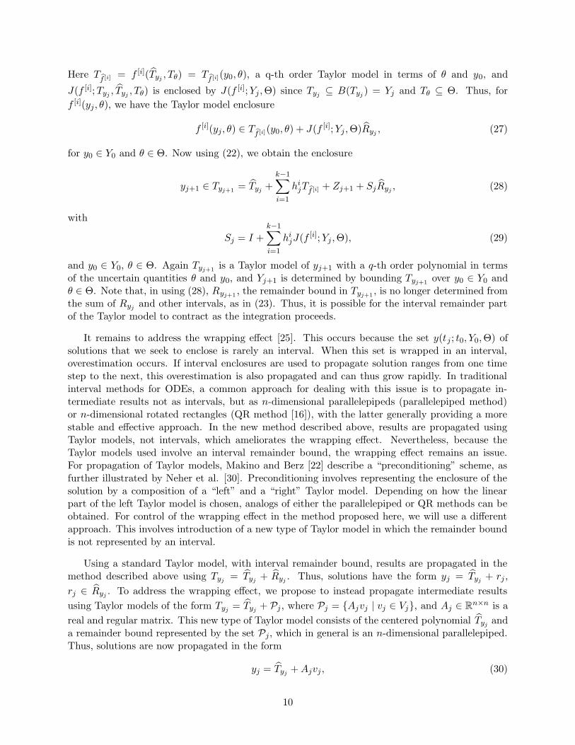
It remains to address the wrapping effect [25]. This occurs because the set y(tj ; t0, Y0,Θ) ofsolutions that we seek to enclose is rarely an interval. When this set is wrapped in an interval,overestimation occurs. If interval enclosures are used to propagate solution ranges from one timestep to the next, this overestimation is also propagated and can thus grow rapidly. In traditionalinterval methods for ODEs, a common approach for dealing with this issue is to propagate in-termediate results not as intervals, but as n-dimensional parallelepipeds (parallelepiped method)or n-dimensional rotated rectangles (QR method [16]), with the latter generally providing a morestable and effective approach. In the new method described above, results are propagated usingTaylor models, not intervals, which ameliorates the wrapping effect. Nevertheless, because theTaylor models used involve an interval remainder bound, the wrapping effect remains an issue.For propagation of Taylor models, Makino and Berz [22] describe a “preconditioning” scheme, asfurther illustrated by Neher et al. [30]. Preconditioning involves representing the enclosure of thesolution by a composition of a “left” and a “right” Taylor model. Depending on how the linearpart of the left Taylor model is chosen, analogs of either the parallelepiped or QR methods can beobtained. For control of the wrapping effect in the method proposed here, we will use a differentapproach. This involves introduction of a new type of Taylor model in which the remainder boundis not represented by an interval.

Using a standard Taylor model, with interval remainder bound, results are propagated in themethod described above using Tyj

= Tyj+ Ryj

. Thus, solutions have the form yj = Tyj+ rj ,

rj ∈ Ryj. To address the wrapping effect, we propose to instead propagate intermediate results

using Taylor models of the form Tyj= Tyj

+ Pj , where Pj = {Ajvj | vj ∈ Vj}, and Aj ∈ Rn×n is a

real and regular matrix. This new type of Taylor model consists of the centered polynomial Tyjand

a remainder bound represented by the set Pj, which in general is an n-dimensional parallelepiped.Thus, solutions are now propagated in the form

yj = Tyj+ Ajvj , (30)

10

vj ∈ Vj, with A0 = I and V0 = 0.

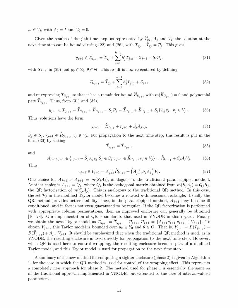
Given the results of the j-th time step, as represented by Tyj, Aj and Vj, the solution at the

next time step can be bounded using (22) and (26), with Tyj− Tyj

= Pj . This gives

yj+1 ∈ Tyj+1 = Tyj+

k−1∑

i=1

hijTf [i] + Zj+1 + SjPj , (31)

with Sj as in (29) and y0 ∈ Y0, θ ∈ Θ. This result is now re-centered by defining

TUj+1 = Tyj+

k−1∑

i=1

hijTf [i] + Zj+1 (32)

and re-expressing TUj+1 so that it has a remainder bound RUj+1 with m(RUj+1) = 0 and polynomial

part TUj+1 . Thus, from (31) and (32),

yj+1 ∈ Tyj+1 = TUj+1 + RUj+1 + SjPj = TUj+1 + RUj+1 + Sj{Ajvj | vj ∈ Vj}. (33)

Thus, solutions have the form

yj+1 = TUj+1 + rj+1 + SjAjvj , (34)

Sj ∈ Sj , rj+1 ∈ RUj+1 , vj ∈ Vj. For propagation to the next time step, this result is put in theform (30) by setting

Tyj+1 = TUj+1 , (35)

andAj+1vj+1 ∈ {rj+1 + SjAjvj|Sj ∈ Sj, rj+1 ∈ RUj+1 , vj ∈ Vj} ⊆ RUj+1 + SjAjVj. (36)

Thus,

vj+1 ∈ Vj+1 = A−1j+1RUj+1 +

(A−1

j+1SjAj

)Vj . (37)

One choice for Aj+1 is Aj+1 = m(SjAj), analogous to the traditional parallelepiped method.Another choice is Aj+1 = Qj, where Qj is the orthogonal matrix obtained from m(SjAj) = QjRj ,the QR factorization of m(SjAj). This is analogous to the traditional QR method. In this case,the set Pj in the modified Taylor model becomes a rotated n-dimensional rectangle. Usually theQR method provides better stability since, in the parallelepiped method, Aj+1 may become illconditioned, and in fact is not even guaranteed to be regular. If the QR factorization is performedwith appropriate column permutations, then an improved enclosure can generally be obtained[16, 28]. Our implementation of QR is similar to that used in VNODE in this regard. Finallywe obtain the next Taylor model as Tyj+1 = Tyj+1 + Pj+1, Pj+1 = {Aj+1vj+1|vj+1 ∈ Vj+1}. Toobtain Yj+1, this Taylor model is bounded over y0 ∈ Y0 and θ ∈ Θ. That is, Yj+1 = B(Tyj+1) =

B(Tyj+1)+Aj+1Vj+1. It should be emphasized that when the traditional QR method is used, as inVNODE, the resulting enclosure is used directly for propagation to the next time step. However,when QR is used here to control wrapping, the resulting enclosure becomes part of a modifiedTaylor model, and this Taylor model is used for propagation to the next time step.

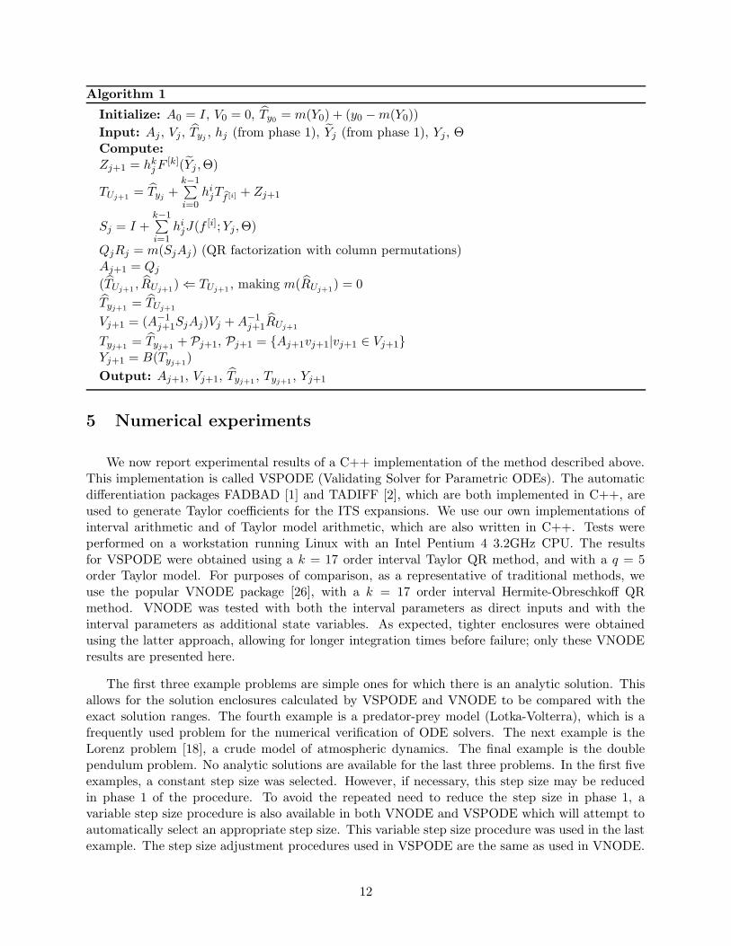
A summary of the new method for computing a tighter enclosure (phase 2) is given in Algorithm1, for the case in which the QR method is used for control of the wrapping effect. This representsa completely new approach for phase 2. The method used for phase 1 is essentially the same asin the traditional approach implemented in VNODE, but extended to the case of interval-valuedparameters.

11

Algorithm 1

Initialize: A0 = I, V0 = 0, Ty0 = m(Y0) + (y0 − m(Y0))

Input: Aj , Vj , Tyj, hj (from phase 1), Yj (from phase 1), Yj, Θ

Compute:

Zj+1 = hkj F

[k](Yj ,Θ)

TUj+1 = Tyj+

k−1∑i=0

hijTf [i] + Zj+1

Sj = I +k−1∑i=1

hijJ(f [i];Yj,Θ)

QjRj = m(SjAj) (QR factorization with column permutations)Aj+1 = Qj

(TUj+1 , RUj+1) ⇐ TUj+1 , making m(RUj+1) = 0

Tyj+1 = TUj+1

Vj+1 = (A−1j+1SjAj)Vj + A−1

j+1RUj+1

Tyj+1 = Tyj+1 + Pj+1, Pj+1 = {Aj+1vj+1|vj+1 ∈ Vj+1}Yj+1 = B(Tyj+1)

Output: Aj+1, Vj+1, Tyj+1 , Tyj+1 , Yj+1

5 Numerical experiments

We now report experimental results of a C++ implementation of the method described above.This implementation is called VSPODE (Validating Solver for Parametric ODEs). The automaticdifferentiation packages FADBAD [1] and TADIFF [2], which are both implemented in C++, areused to generate Taylor coefficients for the ITS expansions. We use our own implementations ofinterval arithmetic and of Taylor model arithmetic, which are also written in C++. Tests wereperformed on a workstation running Linux with an Intel Pentium 4 3.2GHz CPU. The resultsfor VSPODE were obtained using a k = 17 order interval Taylor QR method, and with a q = 5order Taylor model. For purposes of comparison, as a representative of traditional methods, weuse the popular VNODE package [26], with a k = 17 order interval Hermite-Obreschkoff QRmethod. VNODE was tested with both the interval parameters as direct inputs and with theinterval parameters as additional state variables. As expected, tighter enclosures were obtainedusing the latter approach, allowing for longer integration times before failure; only these VNODEresults are presented here.

The first three example problems are simple ones for which there is an analytic solution. Thisallows for the solution enclosures calculated by VSPODE and VNODE to be compared with theexact solution ranges. The fourth example is a predator-prey model (Lotka-Volterra), which is afrequently used problem for the numerical verification of ODE solvers. The next example is theLorenz problem [18], a crude model of atmospheric dynamics. The final example is the doublependulum problem. No analytic solutions are available for the last three problems. In the first fiveexamples, a constant step size was selected. However, if necessary, this step size may be reducedin phase 1 of the procedure. To avoid the repeated need to reduce the step size in phase 1, avariable step size procedure is also available in both VNODE and VSPODE which will attempt toautomatically select an appropriate step size. This variable step size procedure was used in the lastexample. The step size adjustment procedures used in VSPODE are the same as used in VNODE.

12

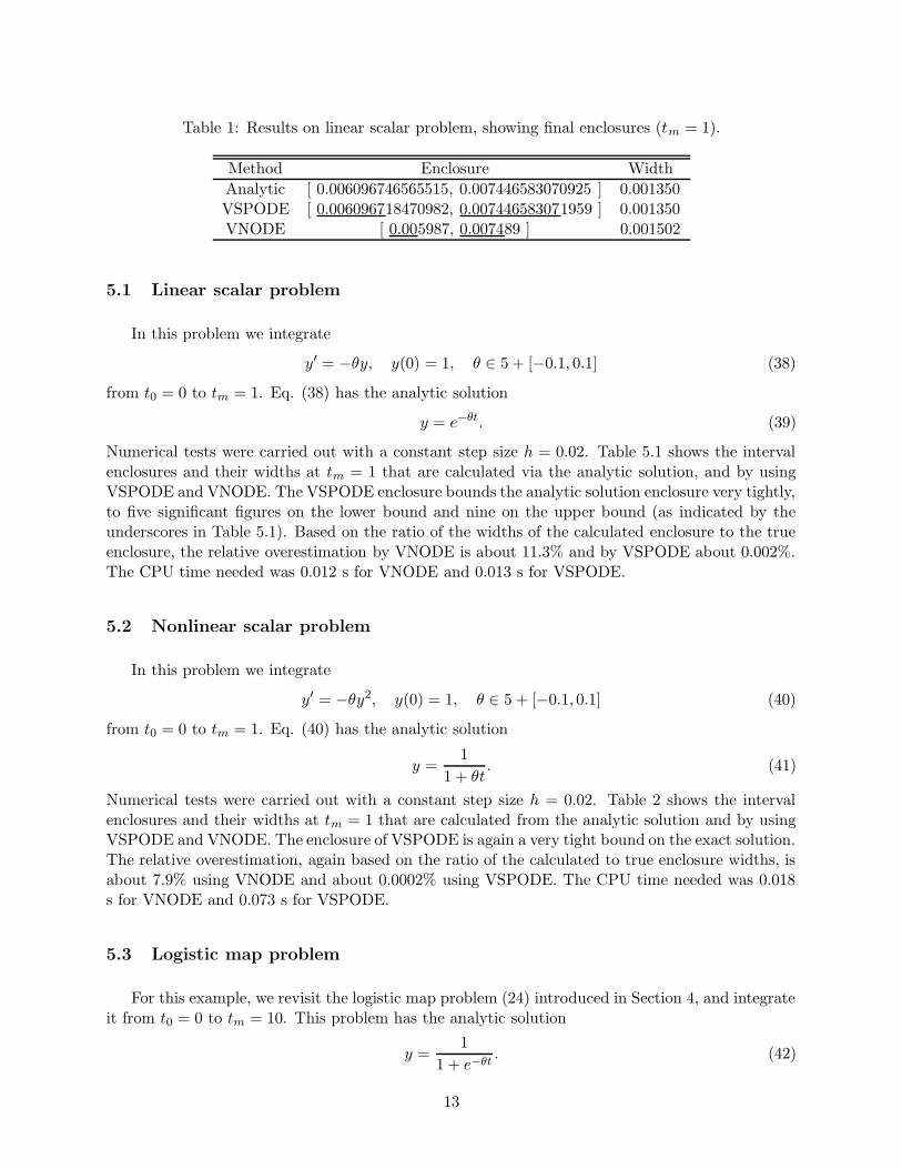
Table 1: Results on linear scalar problem, showing final enclosures (tm = 1).

Method Enclosure Width

Analytic [ 0.006096746565515, 0.007446583070925 ] 0.001350VSPODE [ 0.006096718470982, 0.007446583071959 ] 0.001350VNODE [ 0.005987, 0.007489 ] 0.001502

5.1 Linear scalar problem

In this problem we integrate

y′ = −θy, y(0) = 1, θ ∈ 5 + [−0.1, 0.1] (38)

from t0 = 0 to tm = 1. Eq. (38) has the analytic solution

y = e−θt. (39)

Numerical tests were carried out with a constant step size h = 0.02. Table 5.1 shows the intervalenclosures and their widths at tm = 1 that are calculated via the analytic solution, and by usingVSPODE and VNODE. The VSPODE enclosure bounds the analytic solution enclosure very tightly,to five significant figures on the lower bound and nine on the upper bound (as indicated by theunderscores in Table 5.1). Based on the ratio of the widths of the calculated enclosure to the trueenclosure, the relative overestimation by VNODE is about 11.3% and by VSPODE about 0.002%.The CPU time needed was 0.012 s for VNODE and 0.013 s for VSPODE.

5.2 Nonlinear scalar problem

In this problem we integrate

y′ = −θy2, y(0) = 1, θ ∈ 5 + [−0.1, 0.1] (40)

from t0 = 0 to tm = 1. Eq. (40) has the analytic solution

y =1

1 + θt. (41)

Numerical tests were carried out with a constant step size h = 0.02. Table 2 shows the intervalenclosures and their widths at tm = 1 that are calculated from the analytic solution and by usingVSPODE and VNODE. The enclosure of VSPODE is again a very tight bound on the exact solution.The relative overestimation, again based on the ratio of the calculated to true enclosure widths, isabout 7.9% using VNODE and about 0.0002% using VSPODE. The CPU time needed was 0.018s for VNODE and 0.073 s for VSPODE.

5.3 Logistic map problem

For this example, we revisit the logistic map problem (24) introduced in Section 4, and integrateit from t0 = 0 to tm = 10. This problem has the analytic solution

y =1

1 + e−θt. (42)

13

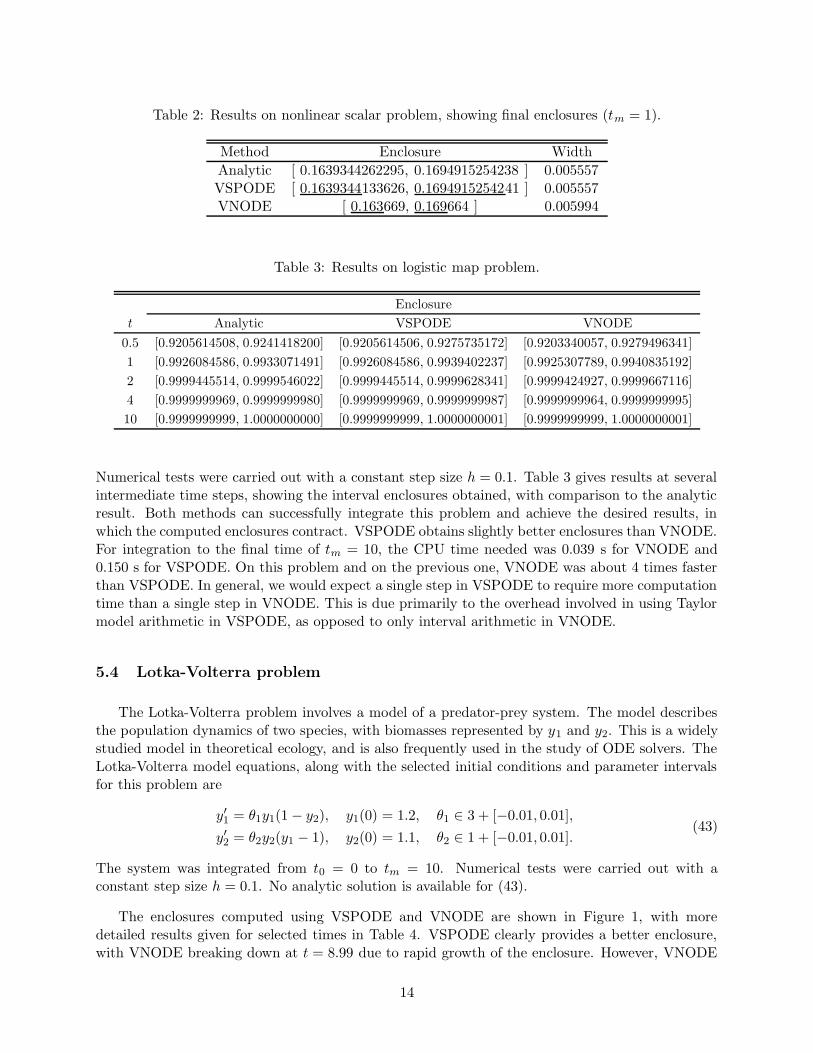
Table 2: Results on nonlinear scalar problem, showing final enclosures (tm = 1).

Method Enclosure Width

Analytic [ 0.1639344262295, 0.1694915254238 ] 0.005557VSPODE [ 0.1639344133626, 0.1694915254241 ] 0.005557VNODE [ 0.163669, 0.169664 ] 0.005994

Table 3: Results on logistic map problem.

Enclosure

t Analytic VSPODE VNODE

0.5 [0.9205614508, 0.9241418200] [0.9205614506, 0.9275735172] [0.9203340057, 0.9279496341]

1 [0.9926084586, 0.9933071491] [0.9926084586, 0.9939402237] [0.9925307789, 0.9940835192]

2 [0.9999445514, 0.9999546022] [0.9999445514, 0.9999628341] [0.9999424927, 0.9999667116]

4 [0.9999999969, 0.9999999980] [0.9999999969, 0.9999999987] [0.9999999964, 0.9999999995]

10 [0.9999999999, 1.0000000000] [0.9999999999, 1.0000000001] [0.9999999999, 1.0000000001]

Numerical tests were carried out with a constant step size h = 0.1. Table 3 gives results at severalintermediate time steps, showing the interval enclosures obtained, with comparison to the analyticresult. Both methods can successfully integrate this problem and achieve the desired results, inwhich the computed enclosures contract. VSPODE obtains slightly better enclosures than VNODE.For integration to the final time of tm = 10, the CPU time needed was 0.039 s for VNODE and0.150 s for VSPODE. On this problem and on the previous one, VNODE was about 4 times fasterthan VSPODE. In general, we would expect a single step in VSPODE to require more computationtime than a single step in VNODE. This is due primarily to the overhead involved in using Taylormodel arithmetic in VSPODE, as opposed to only interval arithmetic in VNODE.

5.4 Lotka-Volterra problem

The Lotka-Volterra problem involves a model of a predator-prey system. The model describesthe population dynamics of two species, with biomasses represented by y1 and y2. This is a widelystudied model in theoretical ecology, and is also frequently used in the study of ODE solvers. TheLotka-Volterra model equations, along with the selected initial conditions and parameter intervalsfor this problem are

y′1 = θ1y1(1 − y2), y1(0) = 1.2, θ1 ∈ 3 + [−0.01, 0.01],

y′2 = θ2y2(y1 − 1), y2(0) = 1.1, θ2 ∈ 1 + [−0.01, 0.01].(43)

The system was integrated from t0 = 0 to tm = 10. Numerical tests were carried out with aconstant step size h = 0.1. No analytic solution is available for (43).

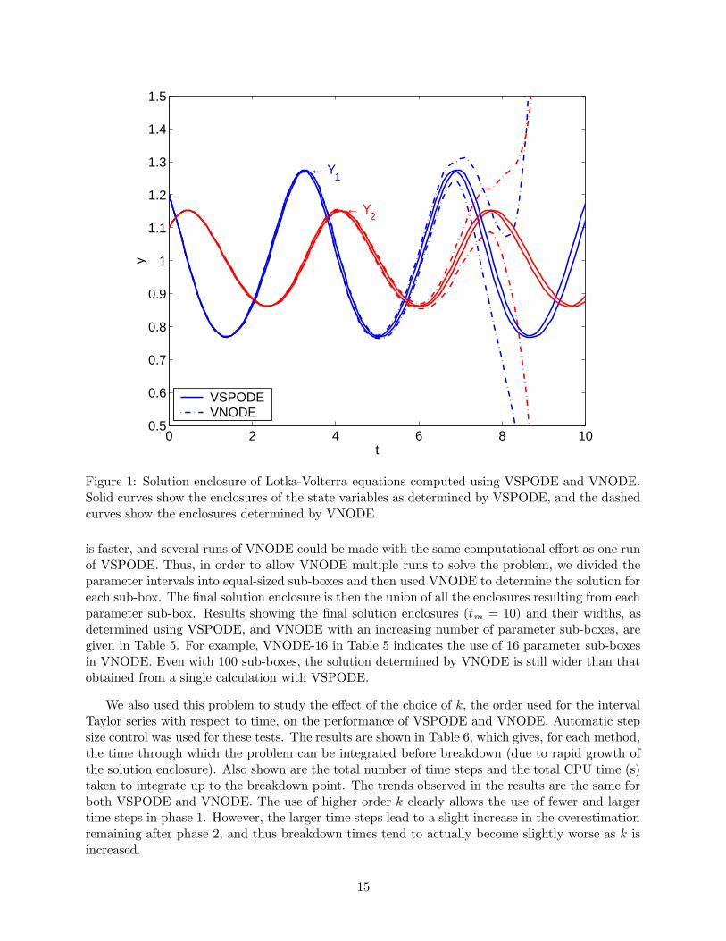
The enclosures computed using VSPODE and VNODE are shown in Figure 1, with moredetailed results given for selected times in Table 4. VSPODE clearly provides a better enclosure,with VNODE breaking down at t = 8.99 due to rapid growth of the enclosure. However, VNODE

14

0 2 4 6 8 100.5

0.6

0.7

0.8

0.9

1

1.1

1.2

1.3

1.4

1.5

t

y

← Y1

← Y2

VSPODEVNODE

Figure 1: Solution enclosure of Lotka-Volterra equations computed using VSPODE and VNODE.Solid curves show the enclosures of the state variables as determined by VSPODE, and the dashedcurves show the enclosures determined by VNODE.

is faster, and several runs of VNODE could be made with the same computational effort as one runof VSPODE. Thus, in order to allow VNODE multiple runs to solve the problem, we divided theparameter intervals into equal-sized sub-boxes and then used VNODE to determine the solution foreach sub-box. The final solution enclosure is then the union of all the enclosures resulting from eachparameter sub-box. Results showing the final solution enclosures (tm = 10) and their widths, asdetermined using VSPODE, and VNODE with an increasing number of parameter sub-boxes, aregiven in Table 5. For example, VNODE-16 in Table 5 indicates the use of 16 parameter sub-boxesin VNODE. Even with 100 sub-boxes, the solution determined by VNODE is still wider than thatobtained from a single calculation with VSPODE.

We also used this problem to study the effect of the choice of k, the order used for the intervalTaylor series with respect to time, on the performance of VSPODE and VNODE. Automatic stepsize control was used for these tests. The results are shown in Table 6, which gives, for each method,the time through which the problem can be integrated before breakdown (due to rapid growth ofthe solution enclosure). Also shown are the total number of time steps and the total CPU time (s)taken to integrate up to the breakdown point. The trends observed in the results are the same forboth VSPODE and VNODE. The use of higher order k clearly allows the use of fewer and largertime steps in phase 1. However, the larger time steps lead to a slight increase in the overestimationremaining after phase 2, and thus breakdown times tend to actually become slightly worse as k isincreased.

15

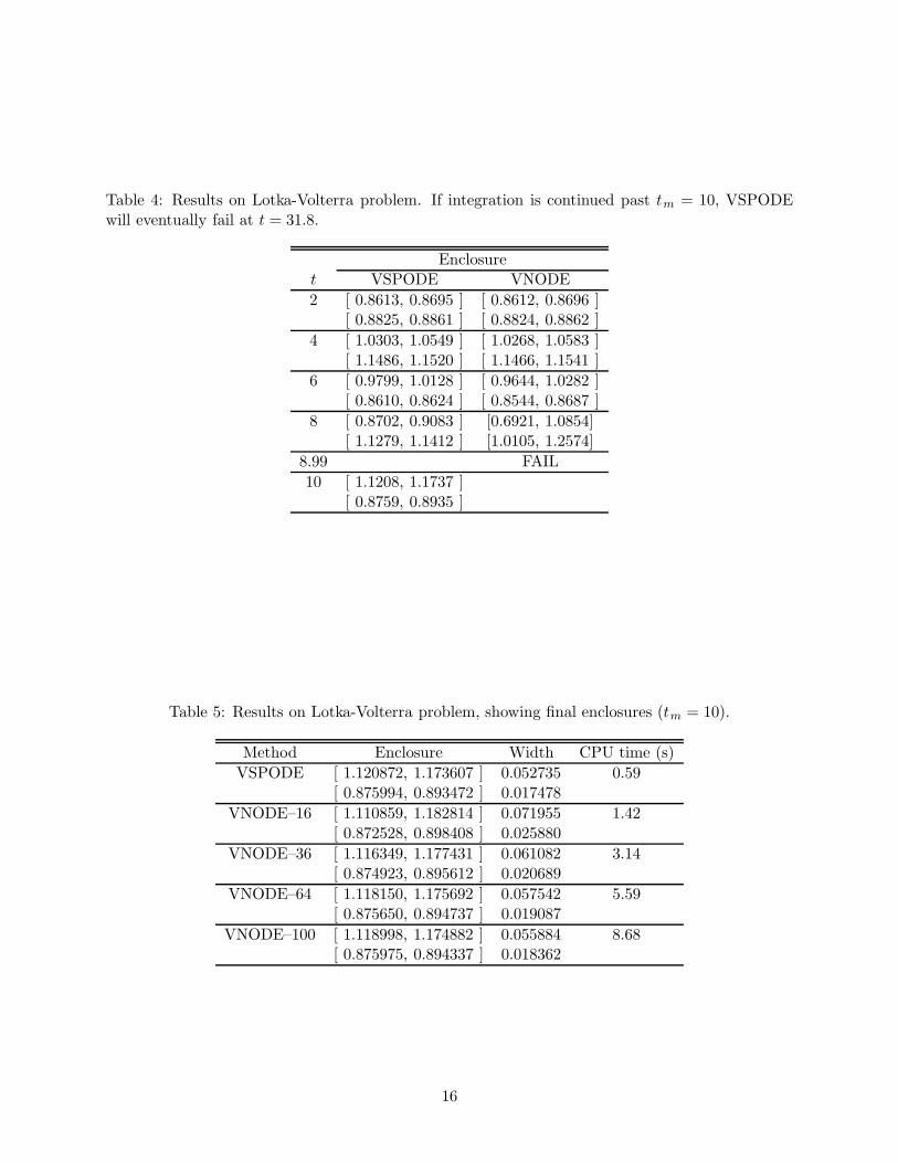
Table 4: Results on Lotka-Volterra problem. If integration is continued past tm = 10, VSPODEwill eventually fail at t = 31.8.

Enclosuret VSPODE VNODE

2 [ 0.8613, 0.8695 ] [ 0.8612, 0.8696 ][ 0.8825, 0.8861 ] [ 0.8824, 0.8862 ]

4 [ 1.0303, 1.0549 ] [ 1.0268, 1.0583 ][ 1.1486, 1.1520 ] [ 1.1466, 1.1541 ]

6 [ 0.9799, 1.0128 ] [ 0.9644, 1.0282 ][ 0.8610, 0.8624 ] [ 0.8544, 0.8687 ]

8 [ 0.8702, 0.9083 ] [0.6921, 1.0854][ 1.1279, 1.1412 ] [1.0105, 1.2574]

8.99 FAIL

10 [ 1.1208, 1.1737 ][ 0.8759, 0.8935 ]

Table 5: Results on Lotka-Volterra problem, showing final enclosures (tm = 10).

Method Enclosure Width CPU time (s)

VSPODE [ 1.120872, 1.173607 ] 0.052735 0.59[ 0.875994, 0.893472 ] 0.017478

VNODE–16 [ 1.110859, 1.182814 ] 0.071955 1.42[ 0.872528, 0.898408 ] 0.025880

VNODE–36 [ 1.116349, 1.177431 ] 0.061082 3.14[ 0.874923, 0.895612 ] 0.020689

VNODE–64 [ 1.118150, 1.175692 ] 0.057542 5.59[ 0.875650, 0.894737 ] 0.019087

VNODE–100 [ 1.118998, 1.174882 ] 0.055884 8.68[ 0.875975, 0.894337 ] 0.018362

16

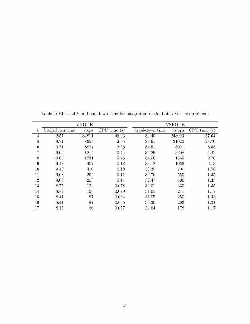
Table 6: Effect of k on breakdown time for integration of the Lotka-Volterra problem.

VNODE VSPODEk breakdown time steps CPU time (s) breakdown time steps CPU time (s)

4 2.57 184811 46.03 33.40 248993 157.645 9.71 8654 2.55 34.61 31020 25.706 9.71 8827 2.65 34.51 8021 8.537 9.65 1214 0.44 34.29 3208 4.428 9.65 1231 0.45 34.06 1666 2.769 9.43 407 0.18 33.72 1066 2.13

10 9.43 410 0.18 33.35 700 1.7811 9.08 202 0.11 32.76 550 1.5512 9.09 203 0.11 32.47 406 1.3313 8.75 124 0.078 32.01 330 1.3514 8.74 125 0.079 31.65 271 1.1715 8.41 87 0.064 31.05 250 1.3316 8.41 87 0.065 30.30 206 1.2117 8.15 66 0.057 29.64 178 1.17

17

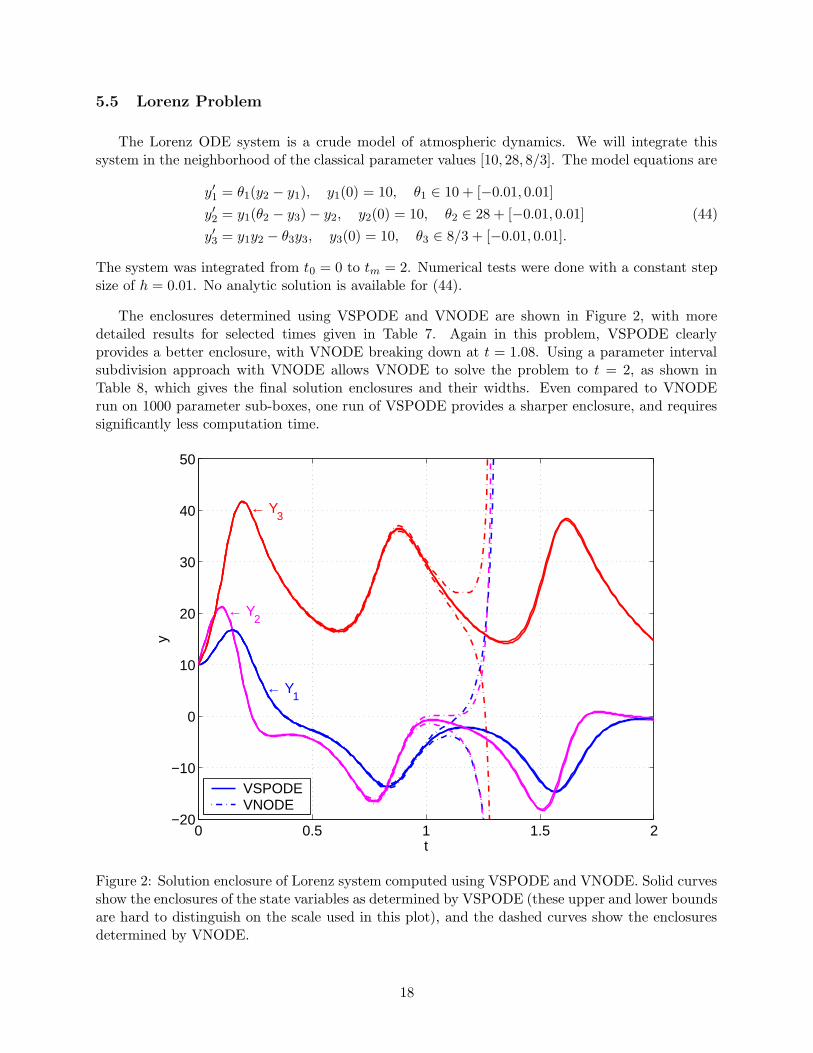
5.5 Lorenz Problem

The Lorenz ODE system is a crude model of atmospheric dynamics. We will integrate thissystem in the neighborhood of the classical parameter values [10, 28, 8/3]. The model equations are

y′1 = θ1(y2 − y1), y1(0) = 10, θ1 ∈ 10 + [−0.01, 0.01]

y′2 = y1(θ2 − y3) − y2, y2(0) = 10, θ2 ∈ 28 + [−0.01, 0.01]

y′3 = y1y2 − θ3y3, y3(0) = 10, θ3 ∈ 8/3 + [−0.01, 0.01].

(44)

The system was integrated from t0 = 0 to tm = 2. Numerical tests were done with a constant stepsize of h = 0.01. No analytic solution is available for (44).

The enclosures determined using VSPODE and VNODE are shown in Figure 2, with moredetailed results for selected times given in Table 7. Again in this problem, VSPODE clearlyprovides a better enclosure, with VNODE breaking down at t = 1.08. Using a parameter intervalsubdivision approach with VNODE allows VNODE to solve the problem to t = 2, as shown inTable 8, which gives the final solution enclosures and their widths. Even compared to VNODErun on 1000 parameter sub-boxes, one run of VSPODE provides a sharper enclosure, and requiressignificantly less computation time.

0 0.5 1 1.5 2−20

−10

0

10

20

30

40

50

t

y

← Y1

← Y2

← Y3

VSPODEVNODE

Figure 2: Solution enclosure of Lorenz system computed using VSPODE and VNODE. Solid curvesshow the enclosures of the state variables as determined by VSPODE (these upper and lower boundsare hard to distinguish on the scale used in this plot), and the dashed curves show the enclosuresdetermined by VNODE.

18

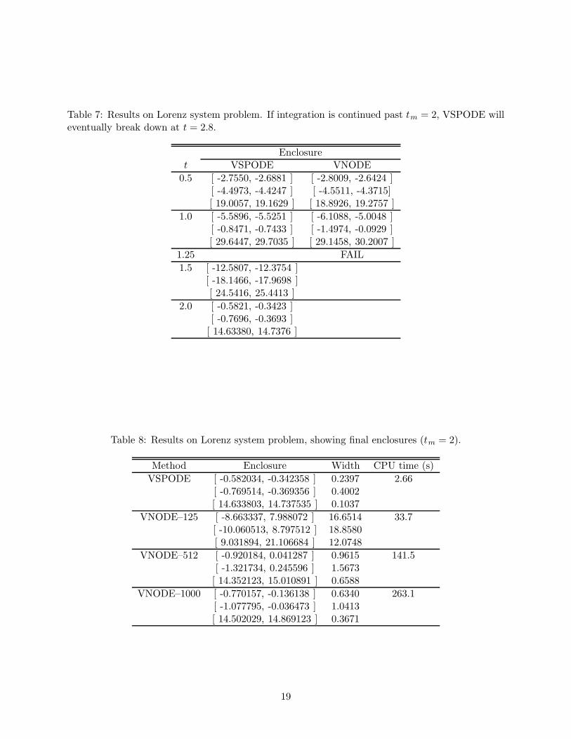
Table 7: Results on Lorenz system problem. If integration is continued past tm = 2, VSPODE willeventually break down at t = 2.8.

Enclosuret VSPODE VNODE

0.5 [ -2.7550, -2.6881 ] [ -2.8009, -2.6424 ][ -4.4973, -4.4247 ] [ -4.5511, -4.3715][ 19.0057, 19.1629 ] [ 18.8926, 19.2757 ]

1.0 [ -5.5896, -5.5251 ] [ -6.1088, -5.0048 ][ -0.8471, -0.7433 ] [ -1.4974, -0.0929 ][ 29.6447, 29.7035 ] [ 29.1458, 30.2007 ]

1.25 FAIL

1.5 [ -12.5807, -12.3754 ][ -18.1466, -17.9698 ][ 24.5416, 25.4413 ]

2.0 [ -0.5821, -0.3423 ][ -0.7696, -0.3693 ]

[ 14.63380, 14.7376 ]

Table 8: Results on Lorenz system problem, showing final enclosures (tm = 2).

Method Enclosure Width CPU time (s)

VSPODE [ -0.582034, -0.342358 ] 0.2397 2.66[ -0.769514, -0.369356 ] 0.4002[ 14.633803, 14.737535 ] 0.1037

VNODE–125 [ -8.663337, 7.988072 ] 16.6514 33.7[ -10.060513, 8.797512 ] 18.8580[ 9.031894, 21.106684 ] 12.0748

VNODE–512 [ -0.920184, 0.041287 ] 0.9615 141.5[ -1.321734, 0.245596 ] 1.5673[ 14.352123, 15.010891 ] 0.6588

VNODE–1000 [ -0.770157, -0.136138 ] 0.6340 263.1[ -1.077795, -0.036473 ] 1.0413[ 14.502029, 14.869123 ] 0.3671

19

m2

m1

2

1

L2

L1

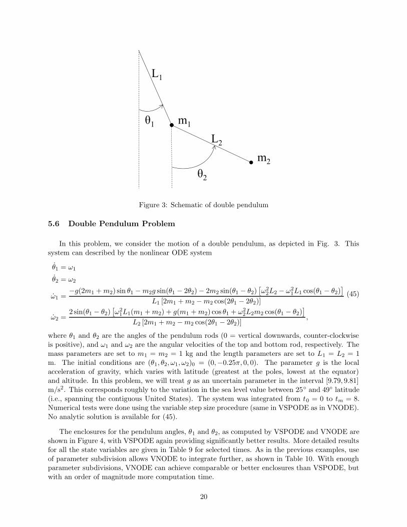
Figure 3: Schematic of double pendulum

5.6 Double Pendulum Problem

In this problem, we consider the motion of a double pendulum, as depicted in Fig. 3. Thissystem can described by the nonlinear ODE system

θ1 = ω1

θ2 = ω2

ω1 =−g(2m1 + m2) sin θ1 − m2g sin(θ1 − 2θ2) − 2m2 sin(θ1 − θ2)

[ω2

2L2 − ω21L1 cos(θ1 − θ2)

]

L1 [2m1 + m2 − m2 cos(2θ1 − 2θ2)]

ω2 =2 sin(θ1 − θ2)

[ω2

1L1(m1 + m2) + g(m1 + m2) cos θ1 + ω22L2m2 cos(θ1 − θ2)

]

L2 [2m1 + m2 − m2 cos(2θ1 − 2θ2)],

(45)

where θ1 and θ2 are the angles of the pendulum rods (0 = vertical downwards, counter-clockwiseis positive), and ω1 and ω2 are the angular velocities of the top and bottom rod, respectively. Themass parameters are set to m1 = m2 = 1 kg and the length parameters are set to L1 = L2 = 1m. The initial conditions are (θ1, θ2, ω1, ω2)0 = (0,−0.25π, 0, 0). The parameter g is the localacceleration of gravity, which varies with latitude (greatest at the poles, lowest at the equator)and altitude. In this problem, we will treat g as an uncertain parameter in the interval [9.79, 9.81]m/s2. This corresponds roughly to the variation in the sea level value between 25◦ and 49◦ latitude(i.e., spanning the contiguous United States). The system was integrated from t0 = 0 to tm = 8.Numerical tests were done using the variable step size procedure (same in VSPODE as in VNODE).No analytic solution is available for (45).

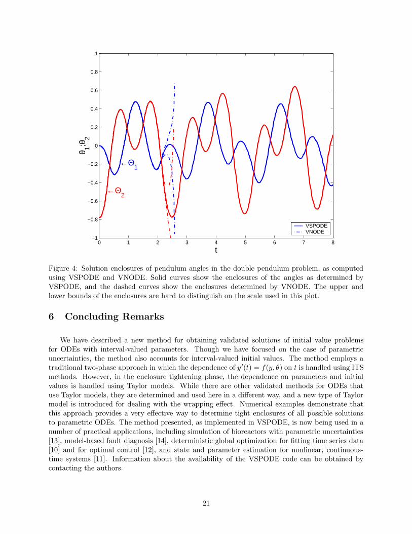
The enclosures for the pendulum angles, θ1 and θ2, as computed by VSPODE and VNODE areshown in Figure 4, with VSPODE again providing significantly better results. More detailed resultsfor all the state variables are given in Table 9 for selected times. As in the previous examples, useof parameter subdivision allows VNODE to integrate further, as shown in Table 10. With enoughparameter subdivisions, VNODE can achieve comparable or better enclosures than VSPODE, butwith an order of magnitude more computation time.

20

0 1 2 3 4 5 6 7 8−1

−0.8

−0.6

−0.4

−0.2

0

0.2

0.4

0.6

0.8

1

t

θ 1;θ2

←Θ1

←Θ2

VSPODEVNODE

Figure 4: Solution enclosures of pendulum angles in the double pendulum problem, as computedusing VSPODE and VNODE. Solid curves show the enclosures of the angles as determined byVSPODE, and the dashed curves show the enclosures determined by VNODE. The upper andlower bounds of the enclosures are hard to distinguish on the scale used in this plot.

6 Concluding Remarks

We have described a new method for obtaining validated solutions of initial value problemsfor ODEs with interval-valued parameters. Though we have focused on the case of parametricuncertainties, the method also accounts for interval-valued initial values. The method employs atraditional two-phase approach in which the dependence of y ′(t) = f(y, θ) on t is handled using ITSmethods. However, in the enclosure tightening phase, the dependence on parameters and initialvalues is handled using Taylor models. While there are other validated methods for ODEs thatuse Taylor models, they are determined and used here in a different way, and a new type of Taylormodel is introduced for dealing with the wrapping effect. Numerical examples demonstrate thatthis approach provides a very effective way to determine tight enclosures of all possible solutionsto parametric ODEs. The method presented, as implemented in VSPODE, is now being used in anumber of practical applications, including simulation of bioreactors with parametric uncertainties[13], model-based fault diagnosis [14], deterministic global optimization for fitting time series data[10] and for optimal control [12], and state and parameter estimation for nonlinear, continuous-time systems [11]. Information about the availability of the VSPODE code can be obtained bycontacting the authors.

21

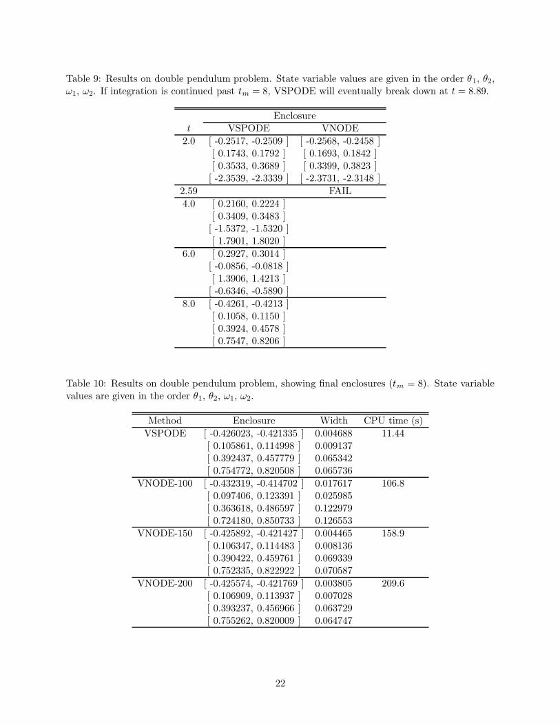
Table 9: Results on double pendulum problem. State variable values are given in the order θ1, θ2,ω1, ω2. If integration is continued past tm = 8, VSPODE will eventually break down at t = 8.89.

Enclosuret VSPODE VNODE

2.0 [ -0.2517, -0.2509 ] [ -0.2568, -0.2458 ][ 0.1743, 0.1792 ] [ 0.1693, 0.1842 ][ 0.3533, 0.3689 ] [ 0.3399, 0.3823 ]

[ -2.3539, -2.3339 ] [ -2.3731, -2.3148 ]

2.59 FAIL

4.0 [ 0.2160, 0.2224 ][ 0.3409, 0.3483 ]

[ -1.5372, -1.5320 ][ 1.7901, 1.8020 ]

6.0 [ 0.2927, 0.3014 ][ -0.0856, -0.0818 ][ 1.3906, 1.4213 ]

[ -0.6346, -0.5890 ]

8.0 [ -0.4261, -0.4213 ][ 0.1058, 0.1150 ][ 0.3924, 0.4578 ][ 0.7547, 0.8206 ]

Table 10: Results on double pendulum problem, showing final enclosures (tm = 8). State variablevalues are given in the order θ1, θ2, ω1, ω2.

Method Enclosure Width CPU time (s)

VSPODE [ -0.426023, -0.421335 ] 0.004688 11.44[ 0.105861, 0.114998 ] 0.009137[ 0.392437, 0.457779 ] 0.065342[ 0.754772, 0.820508 ] 0.065736

VNODE-100 [ -0.432319, -0.414702 ] 0.017617 106.8[ 0.097406, 0.123391 ] 0.025985[ 0.363618, 0.486597 ] 0.122979[ 0.724180, 0.850733 ] 0.126553

VNODE-150 [ -0.425892, -0.421427 ] 0.004465 158.9[ 0.106347, 0.114483 ] 0.008136[ 0.390422, 0.459761 ] 0.069339[ 0.752335, 0.822922 ] 0.070587

VNODE-200 [ -0.425574, -0.421769 ] 0.003805 209.6[ 0.106909, 0.113937 ] 0.007028[ 0.393237, 0.456966 ] 0.063729[ 0.755262, 0.820009 ] 0.064747

22

Acknowledgements

This work was supported in part by the State of Indiana 21st Century Research and Technol-ogy Fund under Grant #909010455, and by the Department of Energy under Grant DE-FG02-05CH11294. The authors also thank Professor George Corliss for reading an earlier draft of thispaper and for making helpful comments and suggestions.

References

[1] C. Bendsten, O. Stauning, FADBAD, a flexible C++ package for automatic differentiationusing the forward and backward methods, Technical Report 1996-x5-94, Technical Universityof Denmark, Lyngby, Denmark (1996).

[2] C. Bendsten, O. Stauning, TADIFF, a flexible C++ package for automatic differentiationusing Taylor series, Technical Report 1997-x5-94, Technical University of Denmark, Lyngby,Denmark (1997).

[3] M. Berz, K. Makino, Verified integration of ODEs and flows using differential algebraic methodson high-order Taylor models, Reliable Computing 4 (1998) 361–369.

[4] G. F. Corliss, R. Rihm, Validating an a priori enclosure using high-order Taylor series, in:G. Alefeld, A. Frommer, B. Lang (eds.), Scientific Computing and Validated Numerics: Pro-ceedings of the International Symposium on Scientific Computing, Computer Arithmetic, andValidated Numerics (SCAN’95), Akademie Verlag, Berlin, Germany (1995).

[5] P. Eijgenraam, The solution of initial value problems using interval arithmetic, Mathemati-cal Centre Tracts No. 144, Stichting Mathematisch Centrum, Amsterdam, The Netherlands(1981).

[6] E. Hansen, G. W. Walster, Global Optimization Using Interval Analysis, Marcel Dekker, NewYork, NY (2004).

[7] M. Janssen, P. V. Hentenryck, Y. Deville, A constraint satisfaction approach for enclosingsolutions to parametric ordinary differential equations, SIAM J. Num. Anal. 40 (2002) 1896–1939.

[8] L. Jaulin, M. Kieffer, O. Didrit, E. Walter, Applied Interval Analysis, Springer-Verlag, London,UK (2001).

[9] R. B. Kearfott, Rigorous Global Search: Continuous Problems, Kluwer Academic Publishers,Dordrecht, The Netherlands (1996).

[10] Y. Lin, M. A. Stadtherr, Deterministic global optimization for parameter estimation of dy-namic systems, Ind. Eng. Chem. Res. (2006) in press.

[11] Y. Lin, M. A. Stadtherr, Guaranteed nonlinear state and parameter estimation for continuous-time systems, Automatica (2006) submitted.

[12] Y. Lin, M. A. Stadtherr, Deterministic global optimization of nonlinear dynamic systems,AIChE J. (2006) submitted.

23

[13] Y. Lin, M. A. Stadtherr, Validated solution of ODEs with parametric uncertainties, Computer-Aided Chem. Eng. 21 (2006) 167–172.

[14] Y. Lin, M. A. Stadtherr, Fault detection in continuous-time systems with uncertain parameters,submitted for presentation at 2007 American Control Conference, New York, NY (2007).

[15] R. J. Lohner, Enclosing the solutions of ordinary initial and boundary value problems, in:C. U. E. Kaucher, U. Kulisch (eds.), Computer Arithmetic: Scientific Computation and Pro-gramming Languages, Teubner, Stuttgart, Germany (1987).

[16] R. J. Lohner, Einschließung der losung gewohnlicher anfangs- und randwertaugfgaben undanwendungen, Ph.D. thesis, Universitat Karlsruhe, Karlsruhe, Germany (1988).

[17] R. J. Lohner, Step size and order control in the verified solution of IVP with ODE’s, in:SciCADE’95 International Conference on Scientific Computation and Differential Equations,Stanford, CA (1995).

[18] E. N. Lorenz, Deterministic non-periodic flow, J. Atmospheric Sci. 20 (1963) 130–141.

[19] K. Makino, Rigorous analysis of nonlinear motion in particle accelerators, Ph.D. thesis, Michi-gan State University, East Lansing, MI (1998).

[20] K. Makino, M. Berz, Remainder differential algebras and their applications, in: M. Berz,C. Bishof, G. Corliss, A. Griewank (eds.), Computational Differentiation: Techniques, Appli-cation, and Tools, SIAM, Philadelphia, PA (1996).

[21] K. Makino, M. Berz, Efficient control of the dependency problem based on Taylor modelmethods, Reliable Computing 5 (1999) 3–12.

[22] K. Makino, M. Berz, Suppression of the wrapping effect by Taylor model-based validatedintegrators, Technical Report MSUHEP 40910, Michigan State University, Lansing, MI (2003).

[23] K. Makino, M. Berz, Taylor models and other validated functional inclusion methods, Int. J.Pure Appl. Math. 4 (2003) 379–456.

[24] K. Makino, M. Berz, Taylor model range bounding schemes, in: Third International Workshopon Taylor Methods, Miami Beach (2004).

[25] R. E. Moore, Interval Analysis, Prentice-Hall, Englewood Cliffs, NJ (1966).

[26] N. S. Nedialkov, Computing rigorous bounds on the solution of an initial value problems for anordinary differential equation, Ph.D. thesis, University of Toronto, Toronto, Canada (1999).

[27] N. S. Nedialkov, K. R. Jackson, Some recent advances in validated methods for IVPs for ODEs,Appl. Numer. Math. 42 (2002) 269–284.

[28] N. S. Nedialkov, K. R. Jackson, G. F. Corliss, Validated solutions of initial value problems forordinary differential equations, Appl. Math. Comput. 105 (1999) 21–68.

[29] N. S. Nedialkov, K. R. Jackson, J. D. Pryce, An effective high-order interval method forvalidating existence and uniqueness of the solution of an IVP for an ODE, Reliable Computing7 (2001) 449–465.

24

[30] M. Neher, K. R. Jackson, N. S. Nedialkov, On Taylor model based integration of ODEs,Technical Report, Department of Computer Science, University of Toronto, Toronto, Canada(2005).

[31] A. Neumaier, Interval Methods for Systems of Equations, Cambridge University Press, Cam-bridge, UK (1990).

[32] A. Neumaier, Taylor forms - use and limits, Reliable Computing 9 (2002) 43–79.

[33] N. Revol, K. Makino, M. Berz, Taylor models and floating point arithmetic: proof that arith-metic operations are bounded in COSY, J. Logic Algebr. Progr. 64 (2005) 135–154.

[34] A. B. Singer, Global dynamic optimization, Ph.D. thesis, Massachusetts Institute of Technol-ogy, Cambridge, MA (2004).

[35] A. B. Singer, P. I. Barton, Bounding the solutions of parameter dependent nonlinear ordinarydifferential equations, SIAM J. Sci. Comput. 27 (2006) 2167–2182.

25