Embed Size (px)
Citation preview

Degree project in
Validation of CIM DC load model forHVDC transmission systems
Georgii ValdenmaiierMehrdad Kazemtabrizi
Stockholm, Sweden 2015
XR-EE-ICS 2015:001
ICSMaster thesis
1
Content
1 Introduction ............................................................................................................................................. 7
1.1 Methodology .......................................................................................................................................................... 7
1.2 Social Contribution ............................................................................................................................................ 8
2 HVDC Overview ................................................................................................................................... 10
2.1 CSC-LCC technology ........................................................................................................................................ 12
2.1.1 Current source converter .................................................................................................................. 12
2.1.2 Line-Commutated CSC Components ............................................................................................ 13
2.1.3 HVDC Link configurations ................................................................................................................. 15
2.1.4 LCC CSC Control methods and levels ........................................................................................... 16
2.1.4.1 LCC Control application............................................................................................................... 17
2.2 VSC Technology ................................................................................................................................................ 19
2.2.1 Voltage source converter................................................................................................................... 20
2.2.2 Multi-level VSC topology .................................................................................................................... 21
2.2.2.1 Three-Level Neutral Point Clamped Converter .............................................................. 21
2.2.2.2 Three-Level Floating Capacitor Topology ......................................................................... 22
2.2.2.3 Series Connection of Converters ............................................................................................ 22
2.2.2.4 Parallel Connection of Converters ......................................................................................... 22
2.2.3 VSC Components .................................................................................................................................... 23
2.2.4 VSC operating configurations .......................................................................................................... 25
2.2.5 VSC CONTROL.......................................................................................................................................... 27
2.2.5.1 Active and Reactive Power Control ....................................................................................... 27
2.2.5.2 Basic PQ Diagram for a VSC Station ...................................................................................... 29
2.2.5.3 Control modes .................................................................................................................................. 29
2.3 Comparison of LCC CSC and VSC converters ..................................................................................... 32
3 CIM overview ........................................................................................................................................ 33
History of CIM ....................................................................................................................................................................... 33
3.1 CIM background ............................................................................................................................................... 35
3.1.1 Technical Committee 57 (TC 57) ................................................................................................... 35
3.1.2 Working Group 13: EMS-API ........................................................................................................... 35
3.1.3 Working Group 14: System Interfaces for Distribution Management ....................... 35
3.1.4 Working Group 16: Deregulated Energy Market Communications ............................ 36
3.1.5 Use cases for CIM ................................................................................................................................... 36
3.1.6 Development Process for CIM data Model ............................................................................... 36
3.2 Technologies in CIM ....................................................................................................................................... 39
3.2.1 Unified Modelling Language (UML) ............................................................................................. 39
3.2.1.1 Class diagrams ................................................................................................................................. 40
3.2.1.2 Package Diagrams .......................................................................................................................... 46
3.2.1.3 Extending UML................................................................................................................................. 48
2
3.2.2 XML Basics ................................................................................................................................................ 48
3.2.2.1 Elements .............................................................................................................................................. 49
3.2.2.2 Character Data and other Markup Elements.................................................................... 49
3.2.2.3 Document Structure ...................................................................................................................... 50
3.2.3 RDF Basics ................................................................................................................................................. 51
3.3 Common Information Model...................................................................................................................... 52
3.3.1 Data Models .............................................................................................................................................. 53
3.3.1.1 IEC 61970-301 (EMS-API) ......................................................................................................... 54
3.3.2 CIM profiles............................................................................................................................................... 54
4 CIM DC Load model ........................................................................................................................... 56
4.1 HVDC Power Flow model description ................................................................................................... 56
4.1.1 HVDC power flow modelling ........................................................................................................... 58
4.1.2 CSC Power Flow model ....................................................................................................................... 60
4.1.3 VSC Power Flow ..................................................................................................................................... 62
4.1.3.1 THE CAPABILITY CURVE OF A VSC TRANSMISSION SYSTEM ................................ 66
4.2 CIM Data Model ................................................................................................................................................. 67
4.2.1 CIM Component Structure ................................................................................................................ 67
4.2.2 UML Proposal .......................................................................................................................................... 72
4.2.2.1 Topology ............................................................................................................................................. 73
4.2.2.2 Containment ...................................................................................................................................... 75
4.2.3 Equipment ................................................................................................................................................. 76
5 jCleanCim ................................................................................................................................................ 78
5.1 jCleanCim configuration ............................................................................................................................... 78
5.1.1 Logging configuration ......................................................................................................................... 79
5.1.2 UML model validation and statistics ........................................................................................... 79
5.1.3 Input and Output Files ........................................................................................................................ 79
5.1.4 MS Word documentation generation .......................................................................................... 80
5.2 The jCleanCim configuration for document generation for IEC 61970-301 ..................... 81
6 Practical Realization of CIM Use .................................................................................................. 84
6.1 Common Information Model for Grid Models Exchange ............................................................. 84
6.2 Exchange Process............................................................................................................................................. 85
6.2.1 Instance File ............................................................................................................................................. 86
6.3 Specifications ..................................................................................................................................................... 87
6.4 Governance of CGMES ................................................................................................................................... 88
6.4.1 Standardisation an interoperability process........................................................................... 89
6.4.2 Approval process ................................................................................................................................... 89
6.4.3 Conformity assessment ...................................................................................................................... 89
6.4.4 Implementation process .................................................................................................................... 89
6.5 Example ................................................................................................................................................................ 89

3
7 Conclusions ........................................................................................................................................... 91
7.1 Future developments ..................................................................................................................................... 92
References .................................................................................................................................................................... 93

4
List of Tables
Table 1. Converter type description ....................................................................................................................... 11
Table 2. Conditions for control strategies in LCC ............................................................................................ 17
Table 3 List of HVDC parameters and variable for simplified power flow model ........................... 59
Table 4 List of CSC parameters and variables for simplified power flow model ............................. 61
Table 5 List of VSC parameters and variables for simplified power flow model ............................. 65
5
List of Figures
Figure 1 Process diagram of the projects including methodology ............................................................. 8
Figure 2. Configuration type of HVDC 3-phase converters ........................................................................ 11
Figure 3. Main types of HVDC Links ....................................................................................................................... 12
Figure 4 6-pulse bridge converter circuit ............................................................................................................. 13
Figure 5 A typical CSC LCC substation terminal ................................................................................................ 13
Figure 6. Electrical control and protection circuit of thyristor level ...................................................... 15
Figure 7. Types of HVDC Link configuration ....................................................................................................... 16
Figure 8 LCC control diagram based on Current margin control ............................................................. 18
Figure 9 Two-level single phase VSC ...................................................................................................................... 20
Figure 10 Three-phase 3-level NPC converter ................................................................................................... 21
Figure 11 Three-phase 3-level floating capacitor converter ...................................................................... 22
Figure 12 Two series-connected six-pulse units .............................................................................................. 22
Figure 13 Two parallel-connected six-pulse units ........................................................................................... 23
Figure 14 VSC substation .............................................................................................................................................. 23
Figure 15 Equivalent circuit of a circuit breaker with closing resistor ................................................ 24
Figure 16 Symmetrical monopolar configuration of VSC Stations .......................................................... 25
Figure 17 Asymmetrical monopolar configuration with metallic return ............................................ 25
Figure 18 Asymmetrical monopolar configuration with ground return .............................................. 25
Figure 19 Bipolar configuration with ground electrodes............................................................................. 26
Figure 20 Bipolar configuration with metallic neutral .................................................................................. 26
Figure 21 Structure of VSC converter ..................................................................................................................... 27
Figure 22 The principle of active power control .............................................................................................. 28
Figure 23 The principle of reactive power control .......................................................................................... 28
Figure 24 A basic simplified PQ diagram .............................................................................................................. 29
Figure 25 VSC Control Scheme ................................................................................................................................... 30
Figure 26 DC voltage droop characteristics ........................................................................................................ 31
Figure 27: CIM electronic model life cycle (CIM book) .................................................................................. 37
Figure 28: Distributed development process of CIM model versions (CIM book) .......................... 38
Figure 29: Possible synchronizations between WGs (CIM book) ............................................................ 38
Figure 30: Example for IEC 61970 model version ........................................................................................... 39
Figure 31: Example of a UML class and an Instance ....................................................................................... 41
Figure 32: UML class........................................................................................................................................................ 41
Figure 33 Connectivity example circuit ................................................................................................................. 42
Figure 34 Example circuit with Connectivity Node ......................................................................................... 42
Figure 35 UML diagram including Connectivity Node an Terminal ...................................................... 43
Figure 36: Associations in UML ................................................................................................................................. 44
6
Figure 37: Aggregation in UML .................................................................................................................................. 44
Figure 38: Composition in UML ................................................................................................................................. 45
Figure 39: Dependency in UML .................................................................................................................................. 45
Figure 40: Generalization in UML ............................................................................................................................. 46
Figure 41: Package in UML ........................................................................................................................................... 46
Figure 42: Different ways of showing elements in a package .................................................................... 47
Figure 43: Package relationships in UML ............................................................................................................. 47
Figure 44: Stereotypes in UML ................................................................................................................................... 48
Figure 45: RDF graph ...................................................................................................................................................... 52
Figure 46: Overview of the CIM standards 61970, 61968, 62325 ........................................................... 53
Figure 47: CIM data base model for IEC 61970-301 ....................................................................................... 54
Figure 48 HVDC bi-polar link from IEC 60633 .................................................................................................. 57
Figure 49 A point-to-point VSC Transmission Scheme ................................................................................. 57
Figure 50 HVDC power flow model ......................................................................................................................... 58
Figure 51 Current Source Converter power flow ............................................................................................. 60
Figure 52 Voltage Source Converter power flow ............................................................................................. 62
Figure 53 VSC unit structure ....................................................................................................................................... 62
Figure 54 Converter symbol identification [15] ............................................................................................... 63
Figure 55 Power flow cases ......................................................................................................................................... 64
Figure 56 Bipolar VSC transmission with earth return ................................................................................. 65
Figure 57 VSC P-Q capability curve ......................................................................................................................... 66
Figure 58: Object instances for symmetric monopole VSC HVDC data model .................................. 68
Figure 59: Object Instances for a bi-polar current source HVDC line .................................................... 70
Figure 60: Containment structure for a bipolar HVDC line ......................................................................... 71
Figure 61: Containment structure for a bipolar back-to-back HVDC station..................................... 72
Figure 62: The basic topology in package Core ................................................................................................. 73
Figure 63: DC and AC topology .................................................................................................................................. 74
Figure 64: HVDC Containment ................................................................................................................................... 75
Figure 65: Equipment model....................................................................................................................................... 76
Figure 66: HVDC line model......................................................................................................................................... 77
Figure 67 Legend for the instance diagrams....................................................................................................... 86
Figure 68 Instance diagram of CSC monopolar configuration ................................................................... 87
Figure 69 Instance diagram of CSC bipolar configuration ........................................................................... 87
Figure 70 CGMES process diagram .......................................................................................................................... 88
Figure 71 Section of HVDC transnission system ............................................................................................... 90
Figure 72 Excerpt of XML file from CGMES ......................................................................................................... 90
7
1 Introduction
The number of cases where the generation is far away from the consumption of electric power is ever growing which led to the development of HVDC transmission as a means for transferring power on long distances. DC technology is nothing brand new but rather was developed before AC power was even realized and eventually replaced DC in power transmission. HVDC was born after the creation of mercury arc valves. The development of mercury arc valves in the 1930s improved the technology and in 1945 a commercial HVDC system in Berlin was commissioned. In 1945 the first commercial HVDC transmission was put into operation with a 96 km sea cable, 20 MW, between the Sweden mainland and the island of Gotland. The converter type that was used in the first HVDC links was the Current Source Converter (CSC) which used line commutation (LCC) by utilizing a thyristor bridge. During the late 1990s, the development of semiconductors for power electronics, such as IGBTs (Insulated Gate Bipolar Transistor) and GTOs (Gate Turn-Off Thyristor), had reached the point where their ratings made it possible to be used for Voltage Source Converters (VSC). “The first commercial VSC based HVDC transmission was first commissioned in 1999 on the island of Gotland with an underground cable of 50 MW. An HVDC system with VSC is also referred to as VSC-HVDC, HVDC Light (by ABB) or HVDC PLUS (Siemens).” [1].
Development in HVDC technology provided the opportunity to create DC grids over the existing AC grids to overcome the problem with transmission bottlenecks prevalent in AC systems. One technology achievement was the creation of high power DC breaker by ABB.
With further growth of HVDC systems, the amount of valuable measurements and parameters needed for managing the power network through SCADA system is increasing substantially. This necessitates accurate data exchange between companies for a slid data base in the SCADA system and efficient analysis. The exchange needs to be translators from the sender and receiver is alleviated. The standard used for this purpose for the AC system led to the creation of Common Information Model (CIM). The constant development of CIM in UML (Unified Modelling Language) made for a detailed model for AC which has been used extensively gathered and documented based on a standard so that the need for in the industry. Ergo, the next rational step would be a similar one for HVDC equipment which was initiated some time ago. The company Ventyx at ABB is a member of the IEC committees responsible for the creation of CIM and maintaining it. A preliminary model has been developed by the committee for HVDC transmission systems.
The main task of this thesis was to validate the preliminary developed model on HVDC and consequently implementing it to the IEC standard 61970-301. The essential objectives can be listed below along with a short description for each:
• Validate the content of CIM DC load model description, which includes formulas and schemes describing VSC, CSC and HVDC power flow, based on academic literature and standards.
• Make compliant the DC model description with UML diagram of CIM DC model in terms of parameters, variables and components.
• Implement the verified DC model description into IEC 61970-301 standard.
• Generate the documentation for IEC 61970-301 with jCleanCim tool.
• Implement the verified CIM DC load model into Network Manager applications.
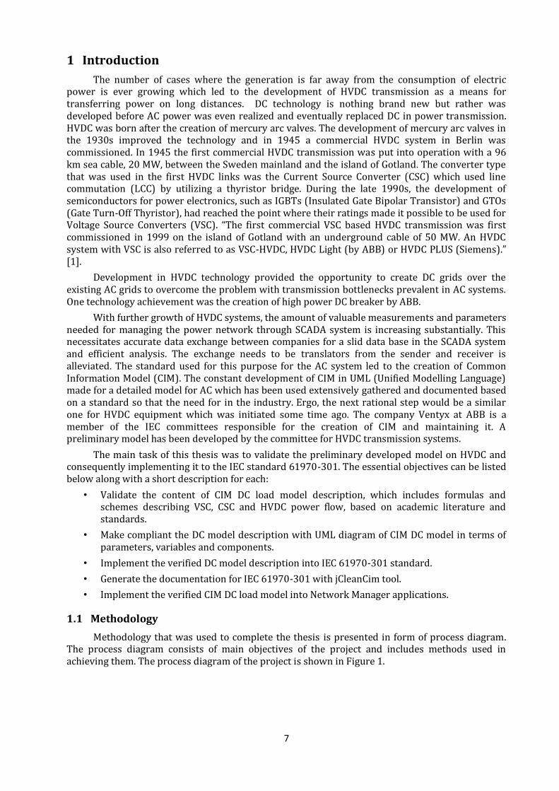
1.1 Methodology
Methodology that was used to complete the thesis is presented in form of process diagram. The process diagram consists of main objectives of the project and includes methods used in achieving them. The process diagram of the project is shown in Figure 1.
8
Validation of DC model description
Academic literature review
IEC reports and standards review
Consultation with industry experts
Validation of UML diagrams for HVDC
model
Adjustment of UML classes parameters with
Validation of CIM data model structure for HVDC
IEC 61970-301 implementation
Extension of the existing standard with validated DC model description
Generating documentation for IEC 61970-301 with jCleanCim tool
Network application implementation
Harmonization of Network Application model with developed CIM DC load
model
Figure 1 Process diagram of the projects including methodology
All 4 objectives shown in Figure 1 were fulfilled, but because of proprietary information included in the last objective about Network application implementation, the results about harmonization of Network application model and CIM DC load model will not be presented in this report.
1.2 Social Contribution
The project has undeniable significant impact on the sustainable development of society. The effect comes from the project’s both main components: HVDC technology and CIM data exchange.
HVDC technology contributions can be realized as the following points:
HVDC can provide fast, precise, and flexible control of transmission flow which substantially improves grid reliability, capacity, and efficiency.
Existing transmission networks are to be developed in order to eliminate transmission bottlenecks and congestions, and furthermore efficiently integrate electrical generation from renewable sources, such as wind and solar.
HVDC transmission technology through stabilizing the power grid, prevents cascading outages that used to cause damage to equipment or destruction of properties and even human fatalities.
Construction of HVDC can be both economically and environmentally beneficial. For longer lines, the cost of HVDC transmission systems is lower than HVAC and indirectly, positively influences the environment, by lower consumption of raw materials and natural resources. Regardless of the line length, HVDC equipment tend to take less space on the building area which reduces the visual impact of the installed equipment.

9
Since the flow of electricity in a DC link is bidirectional, the demand and supply can be balanced more effectively, which also enables power trading.
DC lines have lower power losses than AC lines which results in decrease of power production that eventually reduces the harmful impact caused by electric power generation on the environment.
The standardization of data exchange possesses the following contributions:
An appropriate Information and Communication Technologies (ICT) infrastructure is needed to control the future power type of power transmission and distribution grid and gather relevant data in order to reach a proper interoperability level in the future.
Utilizing a standard method for communication between power companies reduces time and money spent on developing translators to interpret the information being exchanged and extract the data.
The IEC 61970-301/61968 Common Information Model is one of the core standards of the future Smart Grid focused on interoperability. One of the main goals for Smart Grids is to improve the efficiency, reliability, economics, and sustainability of the production and distribution of electricity through permitting the penetration of highly variable renewable energy sources such as wind, solar without the addition of energy storage.
In general the Common Information Model standard is used to provide the means for HVDC transmission utilization and implementation in existing power grids which furthers the development of HVDC technology ultimately resulting in the creation of more opportunities such as funding academic research projects, defining industry focused careers, developing new relative technologies such as power electronics, and extending the scope of renewable energy sources such as wind and solar.

10
2 HVDC Overview
HVDC transmission grids are recently very fast developing field in Power industry. The main reason of the development is their high efficiency – low power loss because of low resistance of transmission lines comparing to AC grids with relative rated power. However applying high-voltage DC grids in power transmission requires breakers and disconnectors that are able to withstand high voltage and high power during switching. That was the main reason why until recent time HVDC lines were used only in point-to-point power links – submarine links, long-distance power links. Development of HVDC breaker by ABB allows applying HVDC technologies not only for point-to-point power links and FACTS, but also building full-scale HVDC transmission grids.
Modern HVDC technologies provide the substantial opportunities [2]:
lack of technical limitations on the length of a submarine cable; possibility to interconnect systems that are not synchronized – back-to-back configuration,
FACTS; no increase in the short-circuit capacity is imposed on the AC systems switchgear; independency of power transfer, set frequency and voltage, phage angle and impedance –
VSC technology; the receiving end of the link may operate in different modes, i.e. it can supply or produce
active or reactive power according to specified criteria (load flow, frequency control, voltage regulation, etc.);
the DC link can be operated to improve the stability of one or both AC systems by modulating the power in response to the power swing etc.
Main advantages of DC Lines:
Higher rated power transmitted per conductor per circuit Smaller tower size in comparison to AC lines Absence of skin effect Lower rate of corona effect and radio interference Lower short circuit fault levels
However HVDC transmission grids are not ideal and possess the drawbacks as well:
o Expensive convertors (for VSC technology even super expensive) o Reactive power requirement – for LCC technology o Generation of harmonics – mainly created by old LCC thyristor-based converters o Difficulty of circuit breaking – high voltage and power during current break o Difficulty of high rated power transmission – power limitation of power electronic
components
Due to complexity and high costs there are 4 main categories of application of HVDC transmission [3]:
Submarine or underground cables Long-distance power transmission (where break-even point is crossed comparing to AC
lines) Asynchronous interconnection of AC systems Stabilization of power flows in integrated power system
Power electronics controller used in HVDC transmission systems can be described as a block of static switches connecting 3 input (output) AC nodes to 2 output (input) DC nodes. The circuits on different sides of the nodes are predominantly inductive or capacitive. Depending on the direction of power flow power electronics controller works in 2 modes:
rectification inversion
There are basically two configuration types of three-phase converters adopted in HVDC systems, which are divided by the main controlling parameter and method of transferring active power:
11
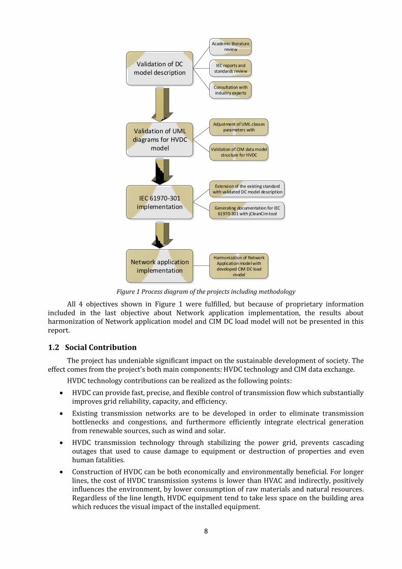
Current Source Converter (CSC) Voltage Source Converter (VSC)
Figure 2. Configuration type of HVDC 3-phase converters
In Table 1 the comparison of main technical features of both converters is presented
Table 1. Converter type description
Converter type CSC VSC
On AC Side
Acts as a constant voltage source Requires a capacitor a its energy storing device Requires large AC filters for harmonic elimination Requires reactive power supply power factor compensation
Acts as a constant current source Requires an inductor as its energy storing device Requires only a small AC filter for higher harmonics elimination Reactive power supply is not required as converter can operate in any quadrant
On DC Side
Acts as a constant current source Requires an inductor as its energy storing device Requires DC filters Provides inherent fault current limiting features
Acts as a constant voltage source Requires a capacitor as its energy storing device Energy storage capacitor provide DC filtering capability at no extra cost Problematic for DC line faults since the charged capacitor will discharge into the fault
Switches Line-commutated or force-commutated with a series capacitor Switching occurs at line frequency (single pulse per cycle) Lower switching loses
Self-commutated Switching occurs at high frequency(multi pulses per cycle) Higher switching loses
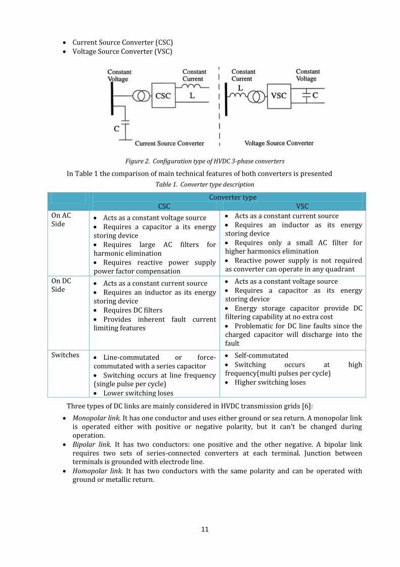
Three types of DC links are mainly considered in HVDC transmission grids [6]:
Monopolar link. It has one conductor and uses either ground or sea return. A monopolar link is operated either with positive or negative polarity, but it can’t be changed during operation.
Bipolar link. It has two conductors: one positive and the other negative. A bipolar link requires two sets of series-connected converters at each terminal. Junction between terminals is grounded with electrode line.
Homopolar link. It has two conductors with the same polarity and can be operated with ground or metallic return.
12
Figure 3. Main types of HVDC Links
2.1 CSC-LCC technology
The most popular type of the commutation process between the converter valves in CSC are line-commutated convertors (LCC). LCC relies on the natural current zeros created by the external circuit for the transfer of current from switch to switch. CSC-LCC technology is the only practical alternative when using semiconductor switches without turn-off capability. It is using the oldest power electronics technology – thyristor–based circuits. But this is still the most common solution currently used in HVDC transmission systems, even though it is the least flexible.
2.1.1 Current source converter
Static converters that are used in HVDC LCC technology has to fulfil the following technical requirements [2]:
Generation of high-quality output waveforms – low rate of noise and absence of low- and high-order harmonics.
Limitation of the dv/dt rate across the switches and other converter components to simplify insulation coordination and reduce RF interference.
High efficiency by reducing on-state and switching losses. Simplicity of the topology – operation stability and reduction of component costs. Flexibility in terms of active and reactive power controllability.
The absence of turn-off controllability of the conventional thyristor results in poor power factors and substantial waveform distortion. Though the LCC configuration is very simple, the external equipment for reactive power compensation and output filtering is complicated and expensive.
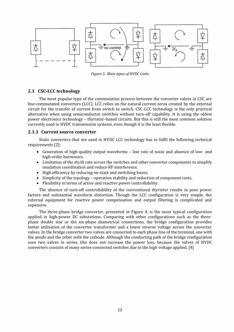
The three-phase bridge converter, presented in Figure 4, is the most typical configuration applied in high-power DC substations. Comparing with other configurations such as the three-phase double star or the six-phase diametrical connections, the bridge configuration provides better utilisation of the converter transformer and a lower inverse voltage across the converter valves. In the bridge converter two valves are connected to each phase line of the terminal, one with the anode and the other with the cathode. Although the conducting path of the bridge configuration uses two valves in series, this does not increase the power loss, because the valves of HVDC converters consists of many series-connected switches due to the high voltage applied. [4]
13
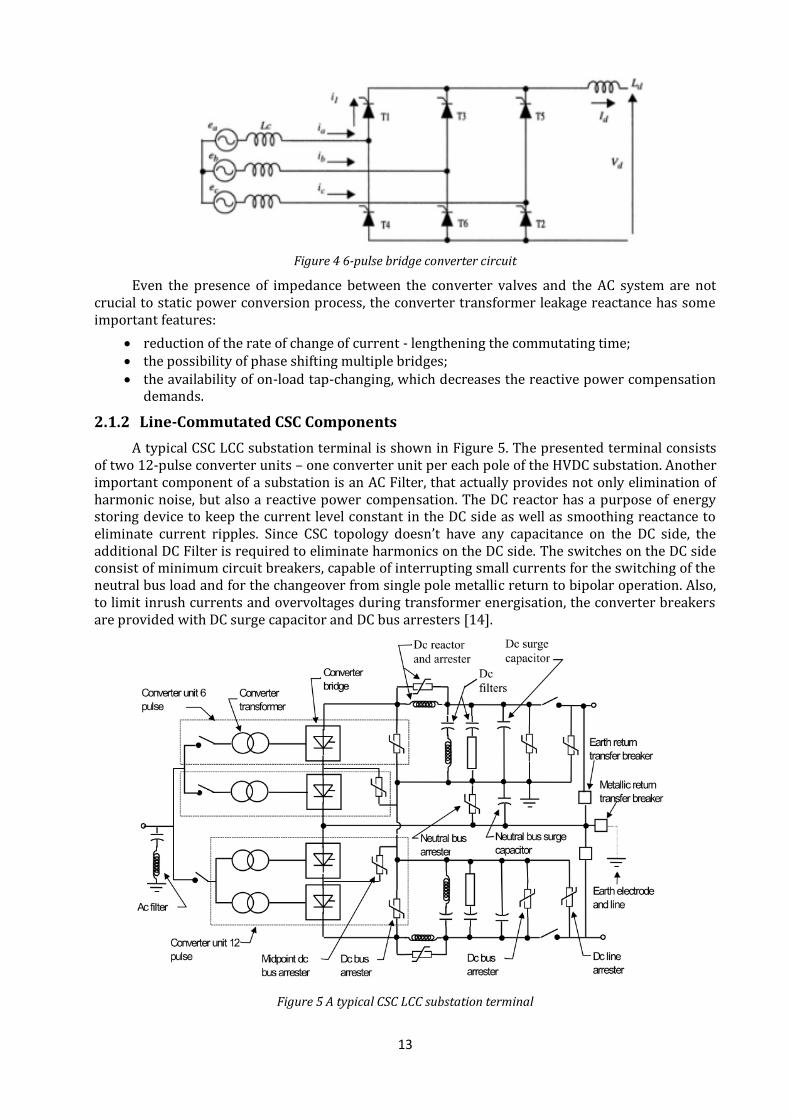
Figure 4 6-pulse bridge converter circuit
Even the presence of impedance between the converter valves and the AC system are not crucial to static power conversion process, the converter transformer leakage reactance has some important features:
reduction of the rate of change of current - lengthening the commutating time; the possibility of phase shifting multiple bridges; the availability of on-load tap-changing, which decreases the reactive power compensation
demands.
2.1.2 Line-Commutated CSC Components
A typical CSC LCC substation terminal is shown in Figure 5. The presented terminal consists of two 12-pulse converter units – one converter unit per each pole of the HVDC substation. Another important component of a substation is an AC Filter, that actually provides not only elimination of harmonic noise, but also a reactive power compensation. The DC reactor has a purpose of energy storing device to keep the current level constant in the DC side as well as smoothing reactance to eliminate current ripples. Since CSC topology doesn’t have any capacitance on the DC side, the additional DC Filter is required to eliminate harmonics on the DC side. The switches on the DC side consist of minimum circuit breakers, capable of interrupting small currents for the switching of the neutral bus load and for the changeover from single pole metallic return to bipolar operation. Also, to limit inrush currents and overvoltages during transformer energisation, the converter breakers are provided with DC surge capacitor and DC bus arresters [14].
Figure 5 A typical CSC LCC substation terminal
14
AC Side Filter
An essential component for providing high-quality output and required reactive power compensation is an AC side filter. During the development of large converter plant, the complex decision is made between using a converter configuration with low levels of waveform distortion and installing harmonic compensation equipment at the terminals to achieve maximum efficiency at minimum cost. The size of a filter is defined as the reactive power that the filter supplies at fundamental frequency. The total size of AC side filter is determined by the reactive power requirement of the harmonic source and by how much this requirement can be supplied by the AC network.
DC Side Filter
On the DC side of LCC converters the voltage harmonics generate current ripples, which amplitudes depend on the delay and extinction angles, the overlap angle and the impedance of DC circuits. The DC Filter possesses the following characteristics:
no fundamental frequency power as a result lower losses; no reactive power, only harmonic mitigation; main capacitor that withstands the full pole-to-neutral DC voltage.
Converter transformer The converter transformers of an LCC substation are usually equipped with on-load tap
changers in order to provide the correct required valve voltage for different load points. Their role is not only to compensate the internal voltage drops of the CSC converters, but deviations in the AC busbar voltage from the base value as well. Another important role of the converter transformer is to limit the short-circuit current.
The converter transformers in LCC technology are mostly of conventional design. They transform the voltage from the AC grid into the one supplied to the DC system. It also provides a separation between the AC and DC system, when the two units of 6-pulse converters are serially connected into 12-pulse converter unit. The standard 12-pulse converter configuration can be obtained with any of the following arrangements:
• six single phase two-winding; • three single phase three-winding; • two three-phase two-winding.
Star or delta connections are equally applied for the above configurations. On-load tap changing is generally used to reduce the demand for the reactive power in the steady state. The range of tap changer varies significantly across each type of application.
The fundamental differences between HVDC and conventional AC transformers are the following [2]:
HVDC transformer insulation to ground and between AC and valve winding has to be designed for combined AC and DC stress.
The valve windings for the HVDC transformer, especially mostly Y-connected valve windings with a relative low number of turns have to be tested with test voltages determined by the protection level of the DC side and not related to the AC (rated) voltage.
HVDC transformer current harmonics cause losses in various parts. DC currents influence the operation of the core and remain unchanged in an HVDC
transformer.
DC smoothing reactors The main purpose of the smoothing reactor is to reduce the rate of rise of the current
following disturbances on either side of the converter. It significantly reduces the number of commutation failures following AC voltage reductions and limits the current peak seen by the rectifying station during DC line short circuits. The second task of the reactor is to decrease the levels of voltage and current harmonics on the DC line and the transfer of non-harmonic frequencies between the two interconnected AC systems.
15
CSC Valve unit
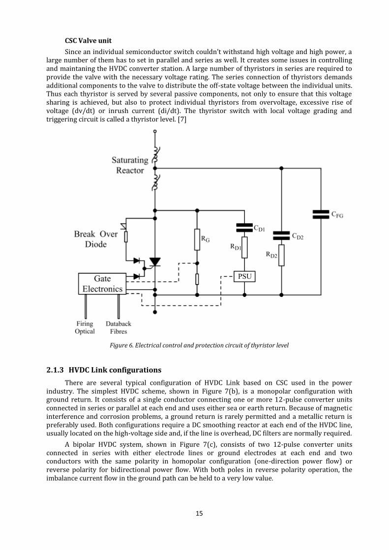
Since an individual semiconductor switch couldn’t withstand high voltage and high power, a large number of them has to set in parallel and series as well. It creates some issues in controlling and maintaning the HVDC converter station. A large number of thyristors in series are required to provide the valve with the necessary voltage rating. The series connection of thyristors demands additional components to the valve to distribute the off-state voltage between the individual units. Thus each thyristor is served by several passive components, not only to ensure that this voltage sharing is achieved, but also to protect individual thyristors from overvoltage, excessive rise of voltage (dv/dt) or inrush current (di/dt). The thyristor switch with local voltage grading and triggering circuit is called a thyristor level. [7]
Figure 6. Electrical control and protection circuit of thyristor level
2.1.3 HVDC Link configurations
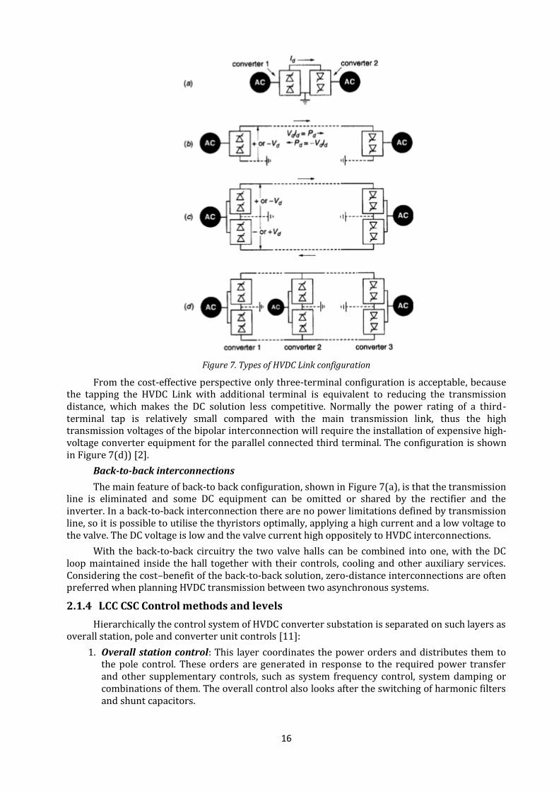
There are several typical configuration of HVDC Link based on CSC used in the power industry. The simplest HVDC scheme, shown in Figure 7(b), is a monopolar configuration with ground return. It consists of a single conductor connecting one or more 12-pulse converter units connected in series or parallel at each end and uses either sea or earth return. Because of magnetic interference and corrosion problems, a ground return is rarely permitted and a metallic return is preferably used. Both configurations require a DC smoothing reactor at each end of the HVDC line, usually located on the high-voltage side and, if the line is overhead, DC filters are normally required.
A bipolar HVDC system, shown in Figure 7(c), consists of two 12-pulse converter units connected in series with either electrode lines or ground electrodes at each end and two conductors with the same polarity in homopolar configuration (one-direction power flow) or reverse polarity for bidirectional power flow. With both poles in reverse polarity operation, the imbalance current flow in the ground path can be held to a very low value.
16
Figure 7. Types of HVDC Link configuration
From the cost-effective perspective only three-terminal configuration is acceptable, because the tapping the HVDC Link with additional terminal is equivalent to reducing the transmission distance, which makes the DC solution less competitive. Normally the power rating of a third-terminal tap is relatively small compared with the main transmission link, thus the high transmission voltages of the bipolar interconnection will require the installation of expensive high-voltage converter equipment for the parallel connected third terminal. The configuration is shown in Figure 7(d)) [2].
Back-to-back interconnections
The main feature of back-to back configuration, shown in Figure 7(a), is that the transmission line is eliminated and some DC equipment can be omitted or shared by the rectifier and the inverter. In a back-to-back interconnection there are no power limitations defined by transmission line, so it is possible to utilise the thyristors optimally, applying a high current and a low voltage to the valve. The DC voltage is low and the valve current high oppositely to HVDC interconnections.
With the back-to-back circuitry the two valve halls can be combined into one, with the DC loop maintained inside the hall together with their controls, cooling and other auxiliary services. Considering the cost–benefit of the back-to-back solution, zero-distance interconnections are often preferred when planning HVDC transmission between two asynchronous systems.
2.1.4 LCC CSC Control methods and levels
Hierarchically the control system of HVDC converter substation is separated on such layers as overall station, pole and converter unit controls [11]:
1. Overall station control: This layer coordinates the power orders and distributes them to the pole control. These orders are generated in response to the required power transfer and other supplementary controls, such as system frequency control, system damping or combinations of them. The overall control also looks after the switching of harmonic filters and shunt capacitors.
17
2. Pole controls: The pole control layer derives the firing order of the pole converters following a power or a DC voltage order.
3. Converter unit controls: This layer is used to control the firing instants of the valves within a bridge and to define the and limits.
The primary functions of the controls in HVDC systems are:
Control power flow between the terminals; Protection of the equipment against the current/voltage stresses caused by faults; Stabilization the attached AC systems against any operational mode of the DC link.
The control of power flow in LCC CSC is provided by controlling in the link. The most used control method used in LCC HVDC link is Current Margin Control method. The method relies on a defined zone of operation of the DC link with proper separation for both terminals and modes – inverter and rectifier 93[22]. Within this control method the LCC terminals can operate in any of the following three modes:
constant current control, constant firing angle (α) control (CFA) or constant extinction angle (γ) control (CEA).
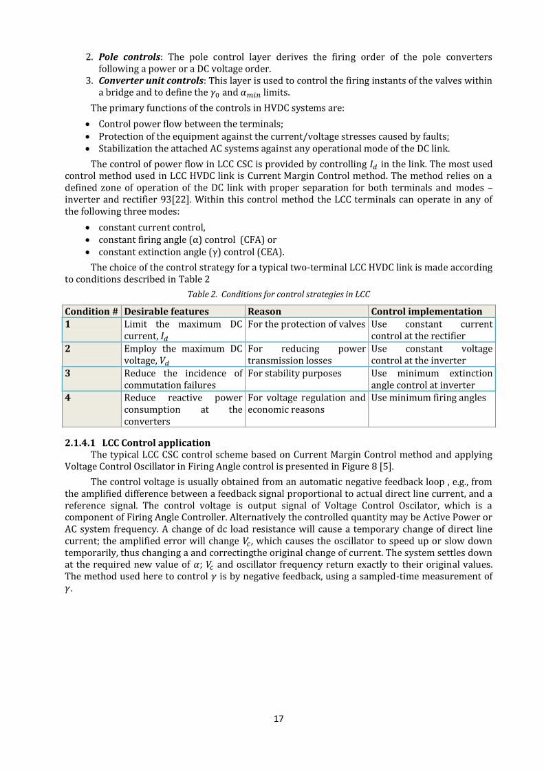
The choice of the control strategy for a typical two-terminal LCC HVDC link is made according to conditions described in Table 2
Table 2. Conditions for control strategies in LCC
Condition # Desirable features Reason Control implementation 1 Limit the maximum DC
current, For the protection of valves Use constant current
control at the rectifier
2 Employ the maximum DC voltage,
For reducing power transmission losses
Use constant voltage control at the inverter
3 Reduce the incidence of commutation failures
For stability purposes Use minimum extinction angle control at inverter
4 Reduce reactive power consumption at the converters
For voltage regulation and economic reasons
Use minimum firing angles
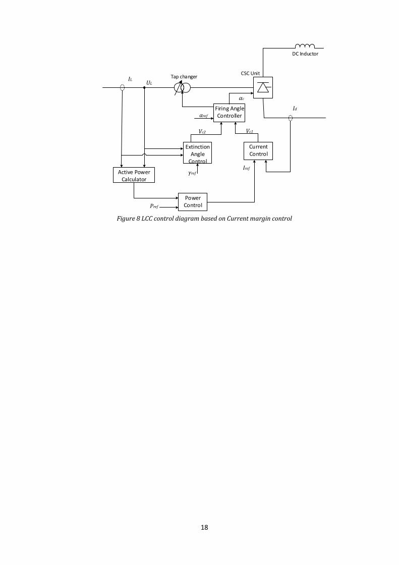
2.1.4.1 LCC Control application The typical LCC CSC control scheme based on Current Margin Control method and applying
Voltage Control Oscillator in Firing Angle control is presented in Figure 8 [5].
The control voltage is usually obtained from an automatic negative feedback loop , e.g., from the amplified difference between a feedback signal proportional to actual direct line current, and a reference signal. The control voltage is output signal of Voltage Control Oscilator, which is a component of Firing Angle Controller. Alternatively the controlled quantity may be Active Power or AC system frequency. A change of dc load resistance will cause a temporary change of direct line current; the amplified error will change , which causes the oscillator to speed up or slow down temporarily, thus changing a and correctingthe original change of current. The system settles down at the required new value of ; and oscillator frequency return exactly to their original values. The method used here to control is by negative feedback, using a sampled-time measurement of .
18
Tap changer
DC Inductor
Active Power Calculator
Current Control
Extinction Angle
Control
Firing Angle Controller
Power Control
CSC Unit
αref
Vc1
αc
Iref
Id
IL UL
Pref
Vc2
γref
Figure 8 LCC control diagram based on Current margin control
19
2.2 VSC Technology
VSC is quite recent HVDC technology developed by ABB as HVDC Light and firstly commissioned in 1999 on 50 MW transmission link between Gotland and continental Sweden.
VSC technology possesses some significant advantages over described LCC CSC technology. First of all VSC is self-commutated technology, that doesn’t require a voltage source for commutation and can operate with zero shirt-circuit ratio (SCR. VSC technology allows generating or absorbing reactive power independently from the active power flow. The maximum transferred active power is limited only by the reactance of the AC system. The necessity of filters in this type of converters is eliminated or reduced to absorb only the higher harmonics, since VSC substantially reduces the generation of harmonics. The low rating of passive filters required by VSC eliminates the issue of overvoltages that cause converter disconnection. The change of power flow direction can be done without the need of switching polarity operations in the terminal.
The most typical applications of VSC in transmission systems are following [3]:
1. The power supply to isolated areas without generating sources, since it omits the need to install expensive synchronous compensators. In this application the inverter terminal controls the fundamental frequency and voltage in the isolated area.
2. The interconnection of two or more synchronous or asynchronous AC systems, where each converter terminal controls its own AC voltage and al others DC power contribution, while the remaining converter controls the DC voltage.
3. The power transfer from an offshore wind farm to an onshore substation. At the wind farm terminal the control of frequency, voltage and power can be coordinated with the generators’ control, as well as with the turbine pitch controller and the wind velocity.
4. The direct connection of generators to DC links avoids the need for generator transformers and AC filters and decreases considerably the switchgear requirements. Voltage control can be exercised entirely by the generator excitation and so converter transformer tap-changers are not required.
In addition to environmental benefits, distributed generation (DG) is also seen as offering important possibilities for improving the quality and security of power supply; it can provide improved reactive power and system voltage control, may avoid losses and user-of-system charges, as well as provide black start capability and the prospect of system islanding.
Power interconnections The liberalisation of the electricity industry relies on power system interconnections to allow
the exchange of power among regions or countries and to transport electrical energy more economically and sustainably over long distances to the load centres. Among the advantages of interconnection are [12]:
• the pooling of generation capability with the opportunity to utilise diverse primary energy resources;
• the creation of larger markets, which enable economies of scale to be realised in the operation of power plants and in accommodating demand growth;
• greater flexibility for the introduction of competition into electricity supply.
Traditionally such advantages have been achieved with AC lines connecting different subsystems, in order to strengthen the interconnection. However, the increasing complexity of power transmission systems has caused the deterioration of the power supply reliability and the number of blackouts in different parts of the world has increased. Therefore developing and strengthening the transmission system is essential step to the reliability of interconnected power systems. The probability of blackouts can be significantly reduced with the back-to-back HVDC interconnections due to their asynchronous mode and controllability.
Possible additional bottlenecks inside the AC systems, resulted from the increased transmitted power, can be avoided by the use of long-distance HVDC links integrated into the system to transmit power directly from remote power generation to load centres.
20
2.2.1 Voltage source converter
The typical VSC converter consists of IGBT modules combined with high-frequency sub-cycle switching carried out by pulse-wide modulation.
The thyristor valve used for the conversion in LCC HVDC can only switch off when the current through it passes zero, and hence relies on the line voltage for commutation. In contrast, the voltage sourced converter is based on controllable semiconductor switches, meaning that the valves can be switched on and off by external low-voltage control signals independently of the main current passing through the valve. This difference in operation gives VSC Transmission significant advantages over LCC HVDC, since the VSC can function when it is connected to an AC system with a very low short-circuit ratio, or even to a passive system without any generation or short-circuit power.
In addition, a significant distortion in the voltage waveshape can lead to a commutation failure for an LCC HVDC scheme, causing a short and temporary interruption in power flow. Because the VSC is self-commutating, it does not suffer from such commutation failures. However, the VSC has diodes connected in anti-parallel to the IGBTs, and in the event of a DC fault, the VSC at both ends must be disconnected by opening the AC circuit breakers and enabling the arc to extinguish.
Because modern semiconductors (IGBT) can be switched on and off several times per cycle, it provides the possibility for switching techniques to produce an output waveshape that won’t contain low order harmonics. The drawback of this technique is the increasing power losses with the switching frequency. However, the better waveshape means that harmonic filtering is easier and the size of the AC filter is significantly reduced.
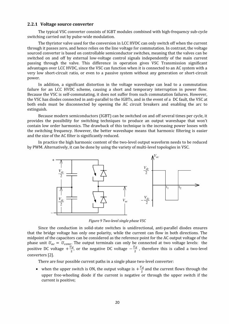
In practice the high harmonic content of the two-level output waveform needs to be reduced by PWM. Alternatively, it can be done by using the variety of multi-level topologies in VSC.
Figure 9 Two-level single phase VSC
Since the conduction in solid-state switches is unidirectional, anti-parallel diodes ensures that the bridge voltage has only one polarity, while the current can flow in both directions. The midpoint of the capacitors can be considered as the reference point for the AC output voltage of the phase unit . The output terminals can only be connected at two voltage levels: the
positive DC voltage
, or the negative DC voltage
, therefore this is called a two-level
converters [2].
There are four possible current paths in a single phase two-level converter:
when the upper switch is ON, the output voltage is
and the current flows through the
upper free-wheeling diode if the current is negative or through the upper switch if the current is positive;
21
when the lower switch is ON, the output voltage is
and the current flows through the
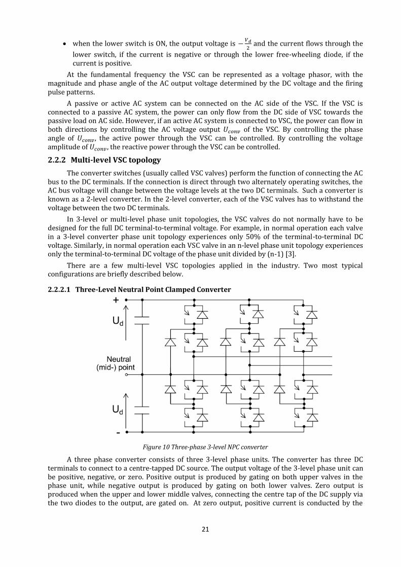
lower switch, if the current is negative or through the lower free-wheeling diode, if the current is positive.
At the fundamental frequency the VSC can be represented as a voltage phasor, with the magnitude and phase angle of the AC output voltage determined by the DC voltage and the firing pulse patterns.
A passive or active AC system can be connected on the AC side of the VSC. If the VSC is connected to a passive AC system, the power can only flow from the DC side of VSC towards the passive load on AC side. However, if an active AC system is connected to VSC, the power can flow in both directions by controlling the AC voltage output of the VSC. By controlling the phase angle of , the active power through the VSC can be controlled. By controlling the voltage amplitude of , the reactive power through the VSC can be controlled.
2.2.2 Multi-level VSC topology
The converter switches (usually called VSC valves) perform the function of connecting the AC bus to the DC terminals. If the connection is direct through two alternately operating switches, the AC bus voltage will change between the voltage levels at the two DC terminals. Such a converter is known as a 2-level converter. In the 2-level converter, each of the VSC valves has to withstand the voltage between the two DC terminals.
In 3-level or multi-level phase unit topologies, the VSC valves do not normally have to be designed for the full DC terminal-to-terminal voltage. For example, in normal operation each valve in a 3-level converter phase unit topology experiences only 50% of the terminal-to-terminal DC voltage. Similarly, in normal operation each VSC valve in an n-level phase unit topology experiences only the terminal-to-terminal DC voltage of the phase unit divided by (n-1) [3].
There are a few multi-level VSC topologies applied in the industry. Two most typical configurations are briefly described below.
2.2.2.1 Three-Level Neutral Point Clamped Converter
Figure 10 Three-phase 3-level NPC converter
A three phase converter consists of three 3-level phase units. The converter has three DC terminals to connect to a centre-tapped DC source. The output voltage of the 3-level phase unit can be positive, negative, or zero. Positive output is produced by gating on both upper valves in the phase unit, while negative output is produced by gating on both lower valves. Zero output is produced when the upper and lower middle valves, connecting the centre tap of the DC supply via the two diodes to the output, are gated on. At zero output, positive current is conducted by the
22
upper-middle controllable device and the upper centre-tap diode, and negative current by the lower-middle controllable and the lower centre-tap diode.
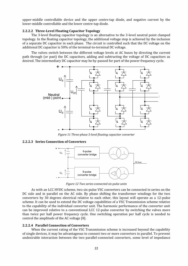
2.2.2.2 Three-Level Floating Capacitor Topology The 3-level floating capacitor topology is an alternative to the 3-level neutral point clamped
topology. In the floating capacitor topology, the additional voltage step is achieved by the inclusion of a separate DC capacitor in each phase. The circuit is controlled such that the DC voltage on the additional DC capacitor is 50% of the terminal-to-terminal DC voltage.
The valves switch between the different voltage levels at AC buses by directing the current path through (or past) the DC capacitors, adding and subtracting the voltage of DC capacitors as desired. The intermediary DC capacitor may be by-passed for part of the power frequency cycle.
Figure 11 Three-phase 3-level floating capacitor converter
2.2.2.3 Series Connection of Converters
Figure 12 Two series-connected six-pulse units
As with an LCC HVDC scheme, two six-pulse VSC converters can be connected in series on the DC side and in parallel on the AC side. By phase shifting the transformer windings for the two converters by 30 degrees electrical relative to each other, this layout will operate as a 12-pulse scheme. It can be used to extend the DC voltage capabilities of a VSC Transmission scheme relative to the capability of the individual converter unit. The harmonic performance of the converter unit can be improved relative to a conventional LCC 12-pulse converter by switching the valves more than twice per half power frequency cycle. One switching operation per half cycle is needed to control the amplitude of the AC voltage [8].
2.2.2.4 Parallel Connection of Converters When the current rating of the VSC Transmission scheme is increased beyond the capability
of single devices, it may be advantageous to connect two or more converters in parallel. To prevent undesirable interaction between the two parallel-connected converters, some level of impedance
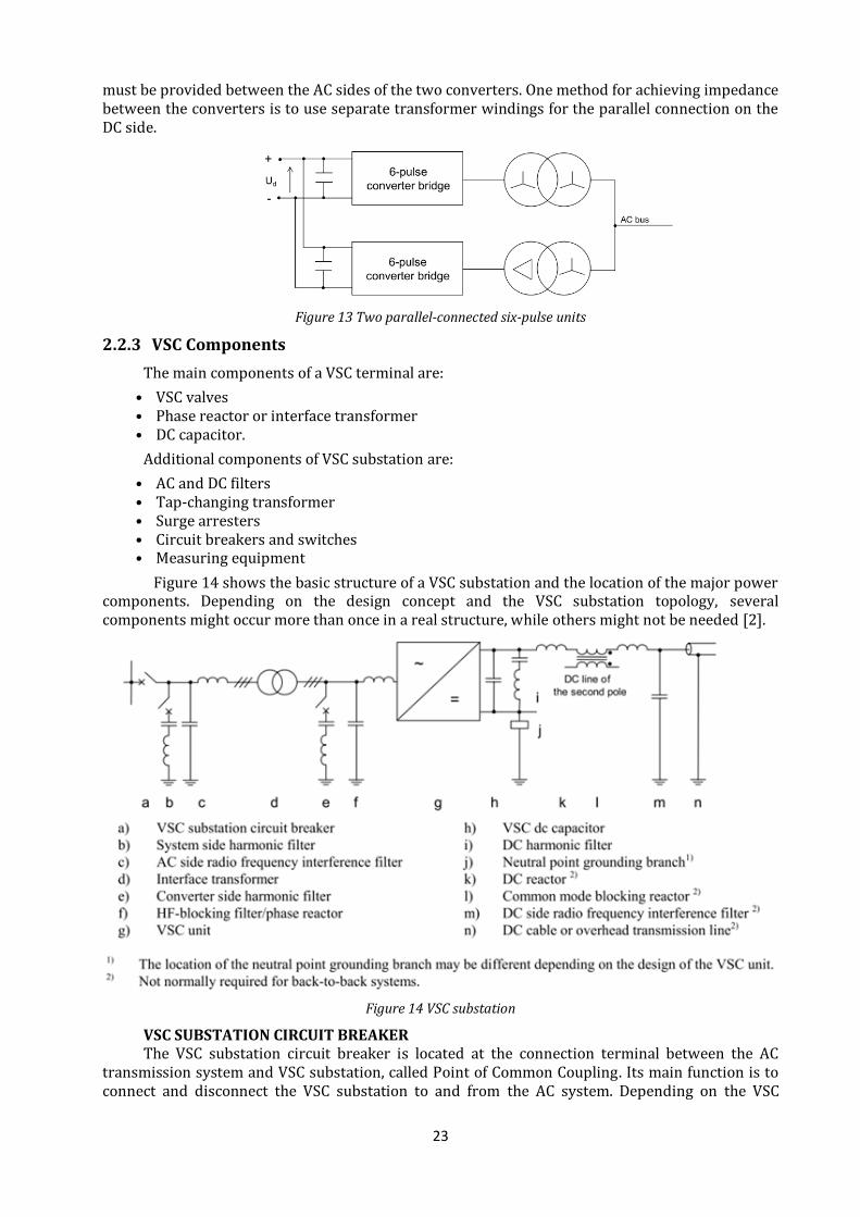
23
must be provided between the AC sides of the two converters. One method for achieving impedance between the converters is to use separate transformer windings for the parallel connection on the DC side.
Figure 13 Two parallel-connected six-pulse units
2.2.3 VSC Components
The main components of a VSC terminal are:
• VSC valves • Phase reactor or interface transformer • DC capacitor.
Additional components of VSC substation are:
• AC and DC filters • Tap-changing transformer • Surge arresters • Circuit breakers and switches • Measuring equipment
Figure 14 shows the basic structure of a VSC substation and the location of the major power components. Depending on the design concept and the VSC substation topology, several components might occur more than once in a real structure, while others might not be needed [2].
Figure 14 VSC substation
VSC SUBSTATION CIRCUIT BREAKER The VSC substation circuit breaker is located at the connection terminal between the AC
transmission system and VSC substation, called Point of Common Coupling. Its main function is to connect and disconnect the VSC substation to and from the AC system. Depending on the VSC

24
Transmission scheme, a circuit breaker can be equipped with a closing resistor. The resistor reduces the charging currents of the DC circuit, resulting in smaller AC system disturbances. A closing resistor also reduces the inrush currents of the transformers and filters during VSC substation energization. The equivalent circuit of a circuit breaker, including a closing resistor, is shown in Figure 15.
Figure 15 Equivalent circuit of a circuit breaker with closing resistor
AC SYSTEM SIDE HARMONIC FILTERS Depending on the design concept of a VSC substation, AC side filtering may be required to
prevent VSC-generated harmonics from penetrating into the AC system. As a side effect, harmonic filters generate reactive power. If the AC system is not capable of absorbing this reactive power, it can be compensated by appropriate control of the VSC, or the use of a shunt reactor. If low-order harmonics are eliminated by appropriate modulation methods or multi-level VSC topologies, filters can be tuned to higher frequencies. Filters with higher frequencies are normally cheaper and more compact.
INTERFACE TRANSFORMERS AND PHASE REACTORS In most cases, the VSC substation design will include interface transformers or phase reactor
to fulfil the following functions:
1. Provide a reactance between the AC system and VSC unit 2. Adapt a standard AC system voltage to a value matching the VSC AC output voltage and
allow optimal utilisation of VSC valve ratings 3. Connect several VSC units together on the AC side that have different DC voltage potentials 4. Prevent zero sequence currents from flowing between the AC system and VSC unit
VSC DC CAPACITOR
The VSC DC capacitor provides the DC voltage necessary to operate the VSC. Main functions of DC capacitor are to attenuate voltage ripples and to keep the voltage level within the limit.
DC FILTER
DC filters can be an alternative to increasing the size of the VSC DC capacitor in cases where critical voltage or current distortion values occur within the DC circuit at a single or a small number of harmonics. DC filters can be connected in parallel to the capacitor to reduce the equivalent impedance of the DC circuit at their tuning frequency in order to prevent harmonic currents from flowing into the DC line or cable.
DC REACTOR
For long distance transmission, a DC reactor can be connected in series to a DC overhead transmission line or cable. It can serve the following purposes:
• Reduce harmonic currents flowing in the DC line or cable • Detune critical resonances within the DC circuit
DC CABLE AND OVERHEAD TRANSMISSION LINES
To transmit electric energy over a distance, both cables and overhead transmission lines can be used for VSC HVDC transmission scheme. Since a VSC doesn’t require the change of DC voltage polarity for bidirectional power flow, the cable does not need to be designed for voltage polarity reversal. This allows new types of cables, such as extruded XLPE DC cables, to be used in long distance VSC Transmission systems [3].
25
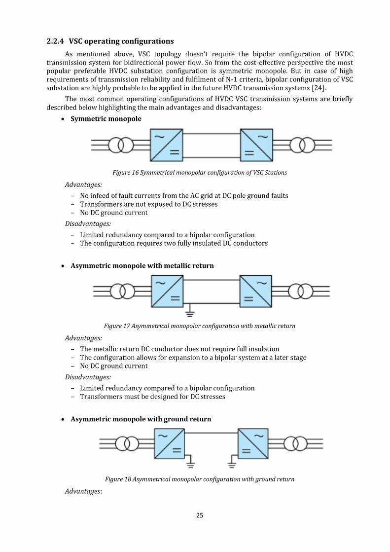
2.2.4 VSC operating configurations
As mentioned above, VSC topology doesn’t require the bipolar configuration of HVDC transmission system for bidirectional power flow. So from the cost-effective perspective the most popular preferable HVDC substation configuration is symmetric monopole. But in case of high requirements of transmission reliability and fulfilment of N-1 criteria, bipolar configuration of VSC substation are highly probable to be applied in the future HVDC transmission systems [24].
The most common operating configurations of HVDC VSC transmission systems are briefly described below highlighting the main advantages and disadvantages:
Symmetric monopole
Figure 16 Symmetrical monopolar configuration of VSC Stations
Advantages:
– No infeed of fault currents from the AC grid at DC pole ground faults – Transformers are not exposed to DC stresses – No DC ground current
Disadvantages:
– Limited redundancy compared to a bipolar configuration – The configuration requires two fully insulated DC conductors
Asymmetric monopole with metallic return
Figure 17 Asymmetrical monopolar configuration with metallic return
Advantages:
– The metallic return DC conductor does not require full insulation – The configuration allows for expansion to a bipolar system at a later stage – No DC ground current
Disadvantages:
– Limited redundancy compared to a bipolar configuration – Transformers must be designed for DC stresses
Asymmetric monopole with ground return
Figure 18 Asymmetrical monopolar configuration with ground return
Advantages:
26
– Cost and losses are minimized due to the single DC conductor – The configuration allows for expansion to a bipolar system at a later stage
Disadvantages:
– Requires permission for continuous operation with DC ground current – Requires permission for electrodes (including environmental effects) – Infeed of fault current from the AC grid at DC pole ground faults – Limited redundancy compared to a bipolar configuration – Transformers must be designed for DC stresses
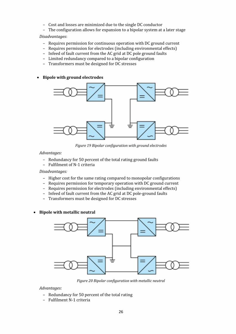
Bipole with ground electrodes
Figure 19 Bipolar configuration with ground electrodes
Advantages:
– Redundancy for 50 percent of the total rating ground faults – Fulfilment of N-1 criteria
Disadvantages:
– Higher cost for the same rating compared to monopolar configurations – Requires permission for temporary operation with DC ground current – Requires permission for electrodes (including environmental effects) – Infeed of fault current from the AC grid at DC pole-ground faults – Transformers must be designed for DC stresses
Bipole with metallic neutral
Figure 20 Bipolar configuration with metallic neutral
Advantages:
– Redundancy for 50 percent of the total rating – Fulfilment N-1 criteria
27
Disadvantages: – Higher cost for the same rating compared to monopolar configurations – Requires low-voltage insulated DC neutral conductor – Transformers must be designed for DC stresses
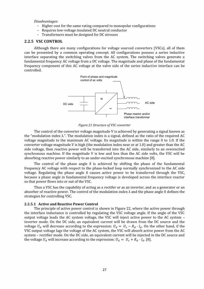
2.2.5 VSC CONTROL
Although there are many configurations for voltage sourced converters (VSCs), all of them can be presented by a common operating concept. All configurations possess a series inductive interface separating the switching valves from the AC system. The switching valves generate a fundamental frequency AC voltage from a DC voltage. The magnitude and phase of the fundamental frequency component of this AC voltage at the valve side of the series inductive interface can be controlled.
Figure 21 Structure of VSC converter
The control of the converter voltage magnitude V is achieved by generating a signal known as the “modulation index λ.”. The modulation index is a signal, defined as the ratio of the required AC voltage magnitude to the maximum AC voltage. Its magnitude is within the range 0 to 1.0. If the converter voltage magnitude V is high (the modulation index near or at 1.0) and greater than the AC side voltage, then reactive power will be transferred into the AC side, similarly to an overexcited synchronous machine. If the magnitude V is low and less than the AC side volts, the VSC will be absorbing reactive power similarly to an under-excited synchronous machine [8].
The control of the phase angle δ is achieved by shifting the phase of the fundamental frequency AC voltage with respect to the phase-locked loop normally synchronized to the AC side voltage. Regulating the phase angle δ causes active power to be transferred through the VSC, because a phase angle in fundamental frequency voltage is developed across the interface reactor so that power flows into or out of the VSC.
Thus a VSC has the capability of acting as a rectifer or as an inverter, and as a generator or an absorber of reactive power. The control of the modulation index λ and the phase angle δ defines the strategies for controlling VSC.
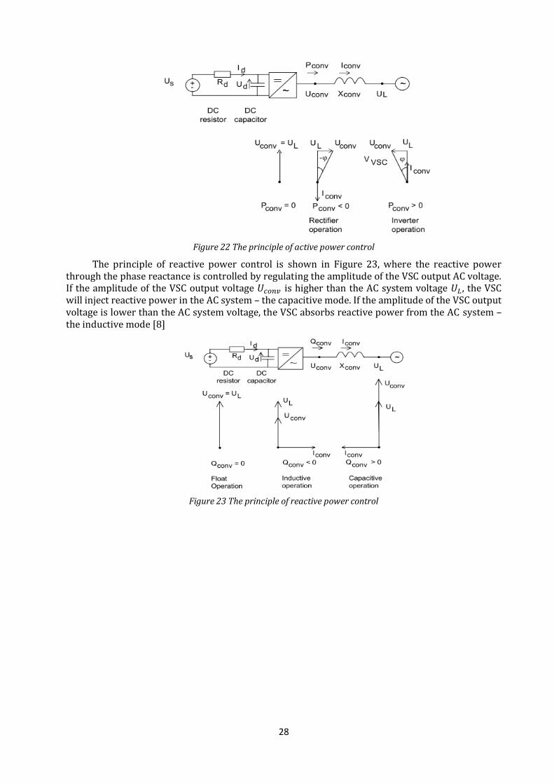
2.2.5.1 Active and Reactive Power Control The principle of active power control is shown in Figure 22, where the active power through
the interface inductance is controlled by regulating the VSC voltage angle. If the angle of the VSC output voltage leads the AC system voltage, the VSC will inject active power to the AC system – inverter mode. On the DC side, an equivalent current will be drawn from the DC source and the voltage will decrease according to the expression: . On the other hand, if the VSC output voltage lags the voltage of the AC system, the VSC will absorb active power from the AC system – rectifier mode. On the DC side, an equivalent current will be injected in the DC source and the voltage will increase according to the expression: . [8].
28
Figure 22 The principle of active power control
The principle of reactive power control is shown in Figure 23, where the reactive power through the phase reactance is controlled by regulating the amplitude of the VSC output AC voltage. If the amplitude of the VSC output voltage is higher than the AC system voltage , the VSC will inject reactive power in the AC system – the capacitive mode. If the amplitude of the VSC output voltage is lower than the AC system voltage, the VSC absorbs reactive power from the AC system – the inductive mode [8]
Figure 23 The principle of reactive power control
29
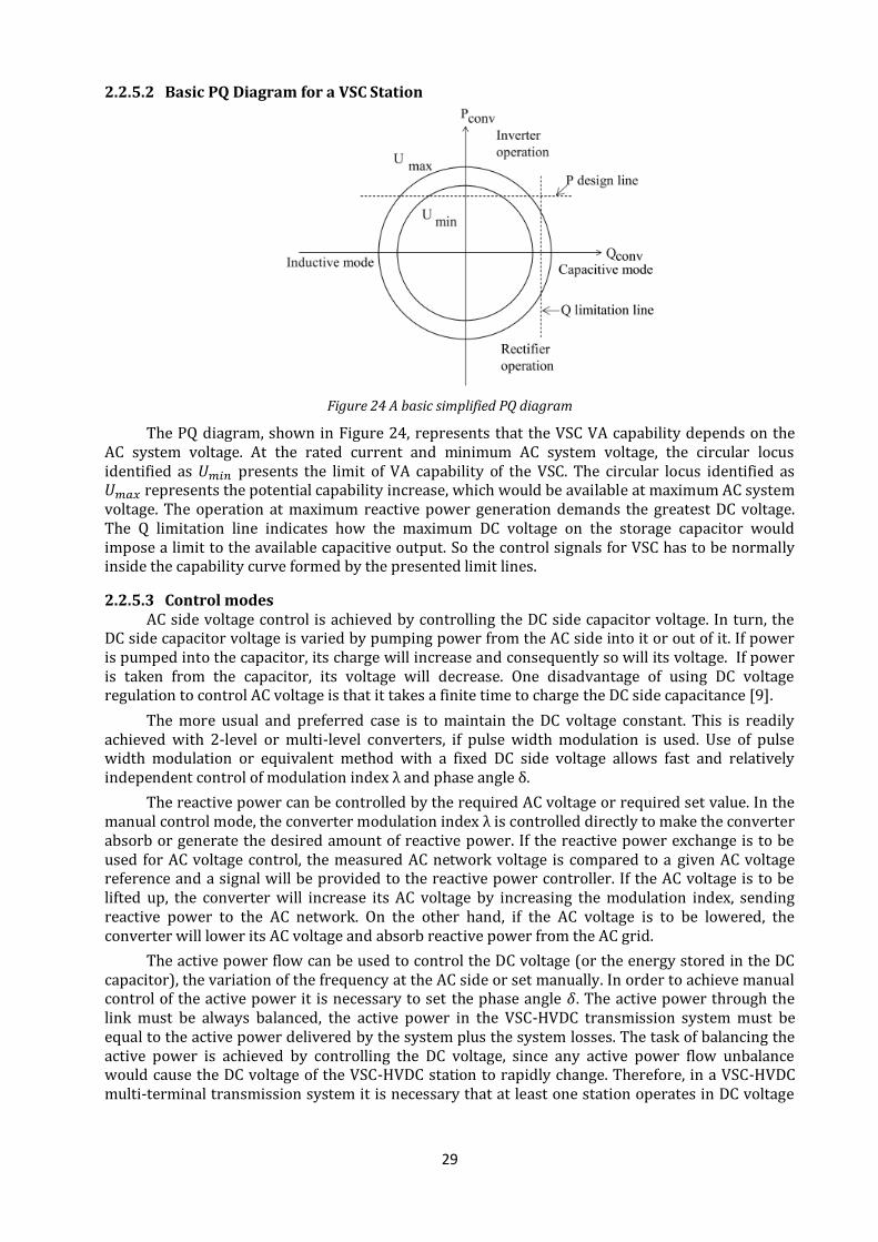
2.2.5.2 Basic PQ Diagram for a VSC Station
Figure 24 A basic simplified PQ diagram
The PQ diagram, shown in Figure 24, represents that the VSC VA capability depends on the AC system voltage. At the rated current and minimum AC system voltage, the circular locus identified as presents the limit of VA capability of the VSC. The circular locus identified as represents the potential capability increase, which would be available at maximum AC system voltage. The operation at maximum reactive power generation demands the greatest DC voltage. The Q limitation line indicates how the maximum DC voltage on the storage capacitor would impose a limit to the available capacitive output. So the control signals for VSC has to be normally inside the capability curve formed by the presented limit lines.
2.2.5.3 Control modes AC side voltage control is achieved by controlling the DC side capacitor voltage. In turn, the
DC side capacitor voltage is varied by pumping power from the AC side into it or out of it. If power is pumped into the capacitor, its charge will increase and consequently so will its voltage. If power is taken from the capacitor, its voltage will decrease. One disadvantage of using DC voltage regulation to control AC voltage is that it takes a finite time to charge the DC side capacitance [9].
The more usual and preferred case is to maintain the DC voltage constant. This is readily achieved with 2-level or multi-level converters, if pulse width modulation is used. Use of pulse width modulation or equivalent method with a fixed DC side voltage allows fast and relatively independent control of modulation index λ and phase angle δ.
The reactive power can be controlled by the required AC voltage or required set value. In the manual control mode, the converter modulation index λ is controlled directly to make the converter absorb or generate the desired amount of reactive power. If the reactive power exchange is to be used for AC voltage control, the measured AC network voltage is compared to a given AC voltage reference and a signal will be provided to the reactive power controller. If the AC voltage is to be lifted up, the converter will increase its AC voltage by increasing the modulation index, sending reactive power to the AC network. On the other hand, if the AC voltage is to be lowered, the converter will lower its AC voltage and absorb reactive power from the AC grid.
The active power flow can be used to control the DC voltage (or the energy stored in the DC capacitor), the variation of the frequency at the AC side or set manually. In order to achieve manual control of the active power it is necessary to set the phase angle . The active power through the link must be always balanced, the active power in the VSC-HVDC transmission system must be equal to the active power delivered by the system plus the system losses. The task of balancing the active power is achieved by controlling the DC voltage, since any active power flow unbalance would cause the DC voltage of the VSC-HVDC station to rapidly change. Therefore, in a VSC-HVDC multi-terminal transmission system it is necessary that at least one station operates in DC voltage
30
control mode, regulating the amount of active power needed to charge or discharge the DC capacitor in order to sustain the required DC voltage level.
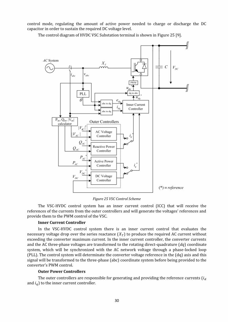
The control diagram of HVDC VSC Substation terminal is shown in Figure 25 [9].
Figure 25 VSC Control Scheme
The VSC-HVDC control system has an inner current control (ICC) that will receive the references of the currents from the outer controllers and will generate the voltages' references and provide them to the PWM control of the VSC.
Inner Current Controller
In the VSC-HVDC control system there is an inner current control that evaluates the necessary voltage drop over the series reactance ( ) to produce the required AC current without exceeding the converter maximum current. In the inner current controller, the converter currents and the AC three-phase voltages are transformed to the rotating direct-quadrature (dq) coordinate system, which will be synchronized with the AC network voltage through a phase-locked loop (PLL). The control system will determinate the converter voltage reference in the (dq) axis and this signal will be transformed to the three-phase (abc) coordinate system before being provided to the converter's PWM control.
Outer Power Controllers
The outer controllers are responsible for generating and providing the reference currents ( and ) to the inner current controller.
31
Using Parks transformation for dq-frame and assuming that the q-axis of the (dq) frame is aligned with the AC network voltage phasor through a PLL, i.e. , active and reactive powers can be presented with following expressions:
DC Voltage Outer Controller
The objective of the DC voltage controller is to maintain the DC voltage at its reference value by regulating the active power exchanged with the AC grid by regulating .
A DC voltage controller that operates on the error between the DC voltage and its reference value
) could be applied, in an analogous way as in the active and reactive power outer controllers. However, if the controller is to operate linearly on the DC voltage, the closed-loop dynamics will be dependent on the operating point.
Voltage Droop Method
The voltage droop method was initially developed for controlling multi-terminal DC networks using HVDC classic technology. However, it can also be applied for grids composed by terminals using VSC technology. In order to guarantee power balance, the method employs a proportional controller which represents a droop characteristic describing a unique relation between the DC voltage and the converter's current (or active power), shown in Figure 26. However, the droop characteristic is valid only for the network topology considered when the droop characteristics were established. Due to this fact the desired operation of the control strategy cannot be achieved using the same droop characteristic if the network topology is changed [9].
Figure 26 DC voltage droop characteristics
The DC voltage droop controller is characterized by power flow which changes linearly with the changes in DC voltage. Differently from the traditional power controllers, where a proportional-integral (PI) regulator is used to compensate steady state errors, thus maintaining the DC voltage at its reference value, this method does not have the ability to keep the DC voltage at a predefined value. If the DC voltage starts to increase, there will be a power surplus in the system and the DC voltage regulating stations should start to increase inversion operation to reestablish power balance. On the other hand, if the DC voltage starts to decrease, that means that there is a lack of power in the system and the DC voltage regulating stations should start to increase rectification. Thus it cause a constant fluctuation and deregulation of active power flow in the transmission system.
Frequency Control
There are two ways to control frequency in VSC:
1. By controlling of the oscillator frequency that determines the valve pulse firing sequence.
2. By regulating active power flow, if the VSC can participate in frequency control.
The ability of a VSC to control frequency and AC voltage, and absorb and deliver real power, makes it useful for assisting in black start conditions.
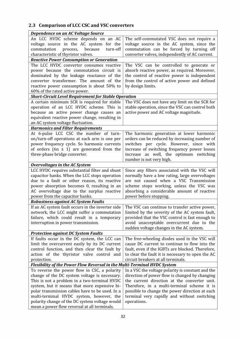
32
2.3 Comparison of LCC CSC and VSC converters
Dependence on an AC Voltage Source An LCC HVDC scheme depends on an AC voltage source in the AC system for the commutation process, because turn-off characteristic of thyristor valves.
The self-commutated VSC does not require a voltage source in the AC system, since the commutation can be forced by turning off converter valves, independently of AC current.
Reactive Power Consumption or Generation The LCC HVDC converter consumes reactive power because the commutation circuit is dominated by the leakage reactance of the converter transformer. The amount of the reactive power consumption is about 50% to 60% of the rated active power.
The VSC can be controlled to generate or absorb reactive power, as required. Moreover, the control of reactive power is independent from the control of active power and defined by design limits.
Short-Circuit Level Requirement for Stable Operation A certain minimum SCR is required for stable operation of an LCC HVDC scheme. This is because an active power change causes an equivalent reactive power change, resulting in an AC system voltage fluctuation.
The VSC does not have any limit on the SCR for stable operation, since the VSC can control both active power and AC voltage magnitude.
Harmonics and Filter Requirements At 6-pulse LCC CSC the number of turn-on/turn-off operations at each arm is one per power frequency cycle. So harmonic currents of orders (6n ± 1) are generated from the three-phase bridge converter.
The harmonic generation at lower harmonic orders can be reduced by increasing number of switches per cycle. However, since with increase of switching frequency power losses increase as well, the optimum switching number is not very high.
Overvoltages in the AC System LCC HVDC requires substantial filter and shunt capacitor banks. When the LCC stops operation due to a fault or other reason, its reactive power absorption becomes 0, resulting in an AC overvoltage due to the surplus reactive power from the capacitor banks.
Since any filters associated with the VSC will normally have a low rating, large overvoltages are not caused when a VSC Transmission scheme stops working, unless the VSC was absorbing a considerable amount of reactive power before stopping.
Robustness against AC System Faults If an AC system fault occurs in the inverter side network, the LCC might suffer a commutation failure, which could result in a temporary interruption in power transmission.
The VSC can continue to transfer active power, limited by the severity of the AC system fault, provided that the VSC control is fast enough to avoid unacceptable overcurrent due to the sudden voltage changes in the AC system.
Protection against DC System Faults If faults occur in the DC system, the LCC can limit the overcurrent easily by its DC current control function, and then clear the fault by action of the thyristor valve control and protection.
The free-wheeling diodes used in the VSC will cause DC current to continue to flow into the fault, even if the IGBTs are blocked. Therefore, to clear the fault it is necessary to open the AC circuit breakers at all terminals.
Flexibility of the Power Flow Reversal in the Multi-Terminal HVDC System To reverse the power flow in CSC, a polarity change of the DC system voltage is necessary. This is not a problem in a two-terminal HVDC system, but it means that more expensive bi-polar transmission cables have to be used. In a multi-terminal HVDC system, however, the polarity change of the DC system voltage would mean a power flow reversal at all terminals.
In a VSC the voltage polarity is constant and the direction of power flow is changed by changing the current direction at the converter unit. Therefore, in a multi-terminal scheme it is possible to change the power direction at each terminal very rapidly and without switching operations.
33
3 CIM overview
History of CIM
In the power system, Energy Management System (EMS), Asset Management System, Work Management System, or Advanced Metering Infrastructure (AMI) use database schemas to define the structure of their storage data which is mostly written in a way to reflect the operator’s specific requirement. Offline applications for performing load-flow, steady state estimation, and fault analysis simulations use the kind of formats for files that is most suitable for that application.
These file formats used for offline analysis are often simple, column-oriented, fixed width, etc. The reason is that the original product coding was marred by hardware limitations such as lack of substantial disk space or memory. So, compactness was always preferred over verbosity to mirror the application’s original data structure (FORTRAN arrays). They are perfectly suitable for data exchange when the required data is only for that particular application. However, extensibility does not fit them very well since the addition of extra items can cause problems such as the software parsing the data could break when finding unknown entries. Compactness of these formats is an advantage and keeps files simple and small and doesn’t take much space, but it also means that formats are not self-describing nor are their documentation publicly available because it is proprietary.[19]
EMS, asset management system and other large-scale applications communicate with each other regularly. As mentioned before, the files being exchanged are all based on the vendor’s own custom format. This means that the user would have to purchase each piece of enterprise software from the same vendor to ensure compatibility during integration or for interface design between different applications.
This need for power companies to exchange data between each other on a daily basis increased drastically after deregulation of the power system. Different power utilities own different parts of a larger power network, so they would have to communicate with each other to ensure the reliable operation of the network. Storage of data in each company is done by using different formats that they deem to be most suitable for their needs. Data is not only exchanged between different companies either as sometimes data has to be sent from one application to another internally.
Due to the aforementioned reason for storing data, exchanging it requires using translators to make it appropriate for transfer. Basically, data needs to be translated once while being exported and another time during import to another application or system. The ordeal gets event more complex when data exchange is between multiple systems and a vast number of applications have to be integrated in order to be ready for the transfer, which creates complications.
In order for the data to be transferred successfully from one vendor’s software application to another or to have multiple versions of the same software running within the company, it can chose one of the following options:
1. Keeping various copies of the same data in different formats. “Keep multiple copies of the
same data in multiple formats.”
2. Storing the data in a format that is compatible with every piece of software. This requires some specific parts of the application to be removed which results in loss of precision.
3. Storing the data in a single format that is greatly detailed and creating translation software
that can turn this particular data format to the one for the desired application.
4. Using a highly detailed format that is compatible with every application and contains the
basic data required for representing the power system while also enabling the containment
of additional, detailed application-specific data without corruption of the original format.
The third option requires the company to invest in additional software engineering to create translation tools but allowing them to have only a single format for all the data. The fourth option is the ideal solution. It enables the company to maintain a single detailed format for data that

34
compatible with any of their software. However, for this option to be achieved, some requirements have to be fulfilled:
1. A highly detailed model would have to be made to describe the power system. 2. A file format would have to be created that is able to store the extended data without
affecting the core data. 3. Power system software vendors and utilities would have to be on board with this data
model and embrace it.
Many standards over the past years were made by various organizations in different countries to address the aforementioned issues and to fulfil the three conditions made above. However, around 2009, the NERC developed a standard that became the unified one for use among all vendors and power companies called the “Common Information Model”.
This model can potentially fulfil the first requirement. The second requirement could be fulfilled by using a means of combining the eXtensible Markup Language (XML) with the Resource Description Framework (RDF). The third requirement is more of a regulatory challenge rather than a technical one. In order for all the vendors and utilities to accept this model unanimously, they would have to acknowledge the benefits that using the standard provides for them. Presently, many major power system application vendors actively participate in the CIM interoperability tests and the popularity of the standard is spreading. CIM is made of different standard formats each with its own purpose.
“The IEC standard 61970-301 is a semantic model that describes the components of a power system at an electrical level and the relationships between each component.” [16]The IEC 61968-11 is an extension to the model that deals with other aspects of the power system software model, such as asset tracking, customer billing, and work scheduling. Both of these models are extended with the IEC 62325-301 that covers data exchange between electricity markets. These three standards are collectively known as The Common Information Model (CIM). CIM is an object-oriented approach for modelling objects. Moreover, it can model the relations between these objects in terms of electrical distribution, transmission, or generation.
Originally developed by the North American Electric Reliability Council (NERC) in the United States to handle exchange of data in the transmission level of the power system, due to the reasons mentioned before, it has grown to a much more complex and comprehensive model now used by the European Network of Transmission Systems Operators for Electricity (ENTSO-E) in Europe and other entities in various countries across Asia.
The CIM was firstly designed to be an EMS-API (Energy Management System, Application Programming Interface, respectively) which its function was to be an internal database model for EMS and SCADA (Supervisory Control and Data Acquisition) system. However, its role soon changed into a much more useful modelling tool of relevant objects and their relations in electric distribution, generation, and transmission aspects, based on the object-oriented modelling approach. Although, it was first designed to address the problem of having a common information model, the CIM’s purpose has grown beyond that initial need. Turning CIM into an international standard was a valid way of promoting it to vendors, not just to utilities. This effort was started by the IEC and chartered the TC 57: Power Management System and Associated Information Exchange. The following drafts for standardization were submitted by TC 57:
Common Information Model (CIM) Generic Interface Definition (GID) Common Power System Model (CPSM)
Working groups were created next to expand the information model. Each working group was assigned a certain sub-area which is shown below:
WG 13 – Energy Management System Application Program Interface (EMS-API)
WG 14 – System Interfaces for Distribution Management (SIDM)
WG 16 – Deregulated Energy Market Communications
WG 19 – Long Term Interoperability within IEC TC 57 Working Groups

35
Each of these working groups designs a set of standards which are assigned a number from IEC and along with their different parts which will be dubbed sub-standards. Among these standards, IEC 61970 and IEC 61968 are the most important ones. CIM is maintained by three of these working groups. It should be mentioned that CIM users group (CIMug) is a forum that was created to feature shared information about the CIM and provide a channel for standards organizations to make suggestions. The organization that continues to conduct research on additional definitions of CIM in other areas and its availability is the EPRI (Electric Power Research Institute) in North America. Another role of the EPRI is to expand the functionality of CIM into other ventures by performing annual interoperability tests.[17]
3.1 CIM background
In this section, the roles of the working groups and different committees formed around CIM are given in more detail.
As it was mentioned in the previous segment, the working groups inside the IEC Technical Committee 57 (TC 57) are maintaining sets of standards so that eventually EMS vendors and all power companies are allowed to exchange data between their applications regardless of their internal software or operating platforms.
3.1.1 Technical Committee 57 (TC 57)
“IEC Technical Committee 57 develops standards for power systems management and associated information exchange.” [17]. In 1965 the committee was established and contains the working groups that were mentioned in the previous section. CIM is maintained by three working groups under IEC TC 57: WG 13, 14, and 16. Working group 19 which is responsible for “Long Term Interoperability within IEC TC 57 Working Groups” harmonizes work among these groups so as to be certain of no duplication of effort to promote interoperability between standards.
3.1.2 Working Group 13: Energy Management System Application Program Interface (EMS-API)
This working group maintains the core CIM as language-independent UML (Unified Model Language) model. In this way, the components of the power system are defined as classes and their relationships as inheritance, association, and aggregation (or composition). More information will be provided about CIM structure later.
In this case, the foundation of the power system is defined as a generic model that can represent all aspects of the power system without relying on proprietary data related to vendor specific equipment or software. So, the interoperability between software applications is simplified to a point of needing only one translator to convert data to CIM format and transferring the data.
The CIM in WG 13 has the functionality of modelling electrical networks from the transmission system operator perspective so it focuses on the electrical network definition and describing applications connected to online operations and analysis of the offline network.
This part of the CIM is published as 61970-301.
3.1.3 Working Group 14: System Interfaces for Distribution Management
This working group maintains the extensions that grew the CIM beyond its original scope to the distribution network and modelling of data exchanged between systems within the distribution utility. So, modelling of unbalanced, low and medium voltage distribution networks were included along with further extensions covering Asset Management, Work Management, Customer Management, Geographical Information Systems (GIS), Maintenance and Construction, Network Planning and a number of other systems. In addition to expanding the scope of CIM with these extensions to include distribution utilities, many can be applied to transmission operators as well.
This part of the CIM is published as IEC 61968-11.

36
3.1.4 Working Group 16: Deregulated Energy Market Communications
As the name suggests, the extensions added to CIM here were done to expand the use of CIM to the area of deregulated energy markets. They include the data required for electricity market operations such as bidding, clearing, and settlement. The data being modelled here is communicated between market players and does not represent the structure of the market itself.
Two primary sub teams exist within this working group, one creating extensions for the European markets and one for the US markets, both have different characteristics.
This part of the CIM is published as IEC 62325-301.
3.1.5 Use cases for CIM
With the growing use of CIM by different vendors, its purpose has become much more than what it was first conceived to be in terms of data model and interface definition. Along with the change in the scope and modelling paradigm, the core applications have also been extended and different use cases have been defined for CIM nowadays:
First use case: using CIM as large domain ontology, one that can provide a vocabulary to express business messages that are exchanged between different system’s utilities. [16]
Second use case: The exchange of topology data using CIM. For different aspects of the power system such as transmission, distribution, CIM profiles (subsets of CIM defining objects and their relations with each other) are used to serialize the power grid schematic in CIM/XML which is based on W3C RDF serialization.
Third use case: Pre-defined processes exist within the CIM models’ structures that can be used as blueprints to use standard-compliant processes and XML schemata. Through XML namespace mechanisms, other utilities or vendor-specific semantics can be added.
Fourth use case: using CIM for purposes related to market and data exchanged with that purpose in different markets whether European or U.S. based markets.
3.1.6 Development Process for CIM data Model
The point of the IEC 61970/61968 standards is to support integration of applications or devices from different vendors. In general, three types of standards that are integration based can be viewed:
1. Standards focusing on syntactic interoperability, providing descriptions for interfaces. 2. Standards focusing on semantic interoperability, which will provide a common semantic
data model in addition to syntactic interoperability. 3. Plug and play standards, the ideal forms of standards which do not require additional
customization and with applications providing specified interfaces, successful exchange of data can be achieved.
The focus of the CIM is on semantic interoperability. Along with a common semantic data model, a set of profiles, interfaces descriptions and use cases are also provided within IEC 61970, 61968, and 62325. The process of developing the IEC CIM data undergoes several steps from its initial inception to the supplying a version of the electronic model.

37
Figure 27: CIM electronic model life cycle (CIM book)
The steps are described in the following:
1. Initial creation: The first version of the CIM, as explained before, was developed based on then existing projects at EPRI. Subsequent versions are being developed until now.
2. Electronic model publication: Documents about CIM are made available on two sides. The current versions as well as selected previous ones of the electronic model of the CIM are provided at the CIMug website as the Enterprise Architect model. The IEC TC 57 hosts all standards as well as the draft versions of further models being developed.
3. Continuous revisions or corrections: After submitting a version of the CIM, it goes under revisions and corrections either taken based on the inputs from the CIMug or other corresponding IEC working groups. CIMug members can submit the modelling issues through the website which will be discussed at IEC modelling team meetings. Further discussions within the modelling team are done usually on a weekly basis. Experts at the TC 57 working groups 13, 14, and 16 comprise the IEC modelling team. Responsibility of certain parts or packages of the CIM is given to their related working groups whereas several working groups use certain parts of the standard. Each working groups has its own modelling manager who coordinates the jobs and responsibilities within the WG and with other working groups.
4. Freezed or combined versions: Publishing the CIM and using requires the version of the standard to be stable. So, versions of the model are freezed. Since different working groups are responsible for developing packages of the CIM, it is necessary to provide combined versions to be used in scenarios that require data exchange between different domains.
Figure 28 shows a typical distributed development process of the CIM model versions within working groups 13, 14, and 16.
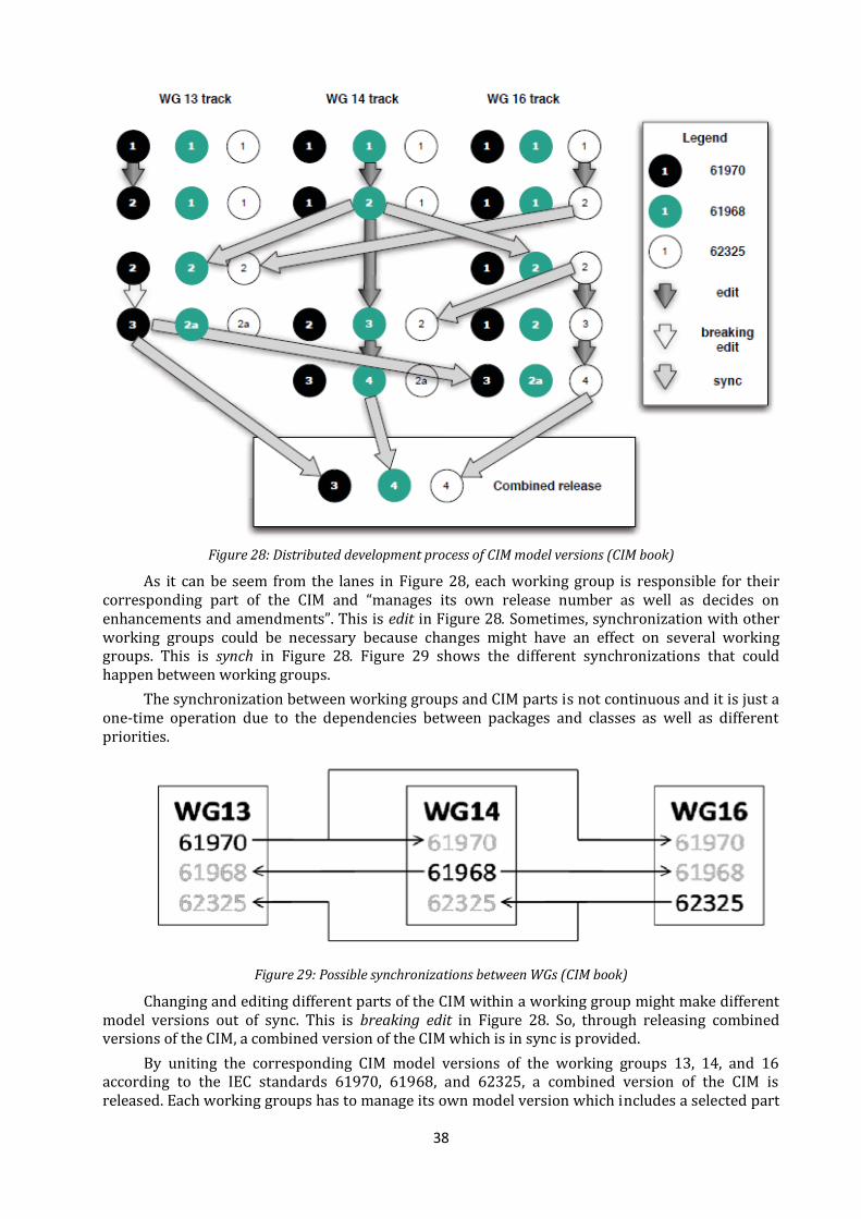
38
Figure 28: Distributed development process of CIM model versions (CIM book)
As it can be seem from the lanes in Figure 28, each working group is responsible for their corresponding part of the CIM and “manages its own release number as well as decides on enhancements and amendments”. This is edit in Figure 28. Sometimes, synchronization with other working groups could be necessary because changes might have an effect on several working groups. This is synch in Figure 28. Figure 29 shows the different synchronizations that could happen between working groups.
The synchronization between working groups and CIM parts is not continuous and it is just a one-time operation due to the dependencies between packages and classes as well as different priorities.
Figure 29: Possible synchronizations between WGs (CIM book)
Changing and editing different parts of the CIM within a working group might make different model versions out of sync. This is breaking edit in Figure 28. So, through releasing combined versions of the CIM, a combined version of the CIM which is in sync is provided.
By uniting the corresponding CIM model versions of the working groups 13, 14, and 16 according to the IEC standards 61970, 61968, and 62325, a combined version of the CIM is released. Each working groups has to manage its own model version which includes a selected part
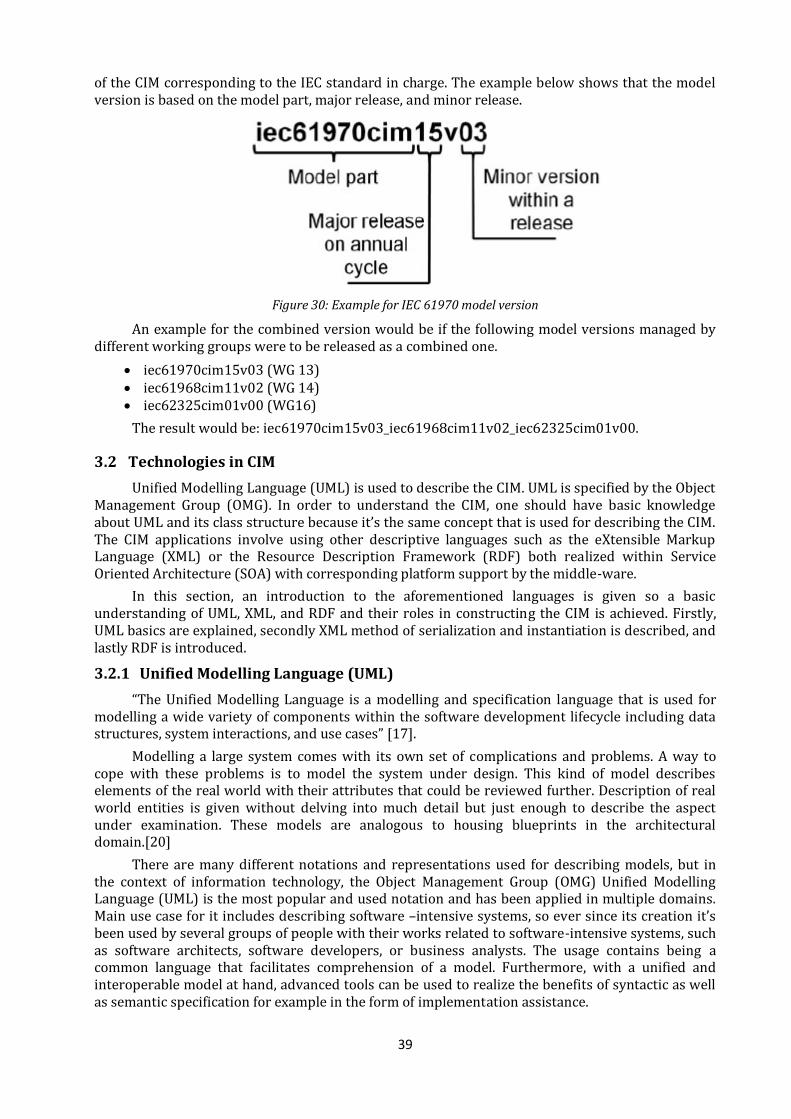
39
of the CIM corresponding to the IEC standard in charge. The example below shows that the model version is based on the model part, major release, and minor release.
Figure 30: Example for IEC 61970 model version
An example for the combined version would be if the following model versions managed by different working groups were to be released as a combined one.
iec61970cim15v03 (WG 13) iec61968cim11v02 (WG 14) iec62325cim01v00 (WG16)
The result would be: iec61970cim15v03_iec61968cim11v02_iec62325cim01v00.
3.2 Technologies in CIM
Unified Modelling Language (UML) is used to describe the CIM. UML is specified by the Object Management Group (OMG). In order to understand the CIM, one should have basic knowledge about UML and its class structure because it’s the same concept that is used for describing the CIM. The CIM applications involve using other descriptive languages such as the eXtensible Markup Language (XML) or the Resource Description Framework (RDF) both realized within Service Oriented Architecture (SOA) with corresponding platform support by the middle-ware.
In this section, an introduction to the aforementioned languages is given so a basic understanding of UML, XML, and RDF and their roles in constructing the CIM is achieved. Firstly, UML basics are explained, secondly XML method of serialization and instantiation is described, and lastly RDF is introduced.
3.2.1 Unified Modelling Language (UML)
“The Unified Modelling Language is a modelling and specification language that is used for modelling a wide variety of components within the software development lifecycle including data structures, system interactions, and use cases” [17].
Modelling a large system comes with its own set of complications and problems. A way to cope with these problems is to model the system under design. This kind of model describes elements of the real world with their attributes that could be reviewed further. Description of real world entities is given without delving into much detail but just enough to describe the aspect under examination. These models are analogous to housing blueprints in the architectural domain.[20]
There are many different notations and representations used for describing models, but in the context of information technology, the Object Management Group (OMG) Unified Modelling Language (UML) is the most popular and used notation and has been applied in multiple domains. Main use case for it includes describing software –intensive systems, so ever since its creation it’s been used by several groups of people with their works related to software-intensive systems, such as software architects, software developers, or business analysts. The usage contains being a common language that facilitates comprehension of a model. Furthermore, with a unified and interoperable model at hand, advanced tools can be used to realize the benefits of syntactic as well as semantic specification for example in the form of implementation assistance.
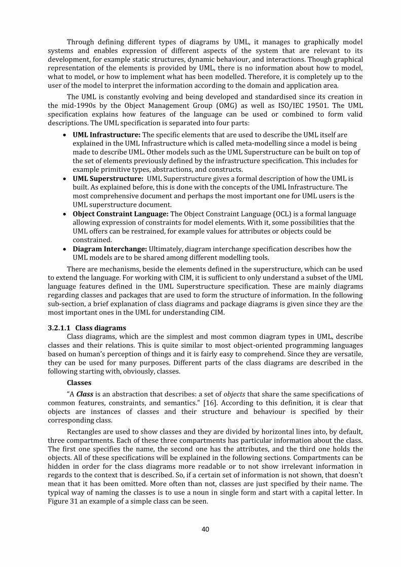
40
Through defining different types of diagrams by UML, it manages to graphically model systems and enables expression of different aspects of the system that are relevant to its development, for example static structures, dynamic behaviour, and interactions. Though graphical representation of the elements is provided by UML, there is no information about how to model, what to model, or how to implement what has been modelled. Therefore, it is completely up to the user of the model to interpret the information according to the domain and application area.
The UML is constantly evolving and being developed and standardised since its creation in the mid-1990s by the Object Management Group (OMG) as well as ISO/IEC 19501. The UML specification explains how features of the language can be used or combined to form valid descriptions. The UML specification is separated into four parts:
UML Infrastructure: The specific elements that are used to describe the UML itself are explained in the UML Infrastructure which is called meta-modelling since a model is being made to describe UML. Other models such as the UML Superstructure can be built on top of the set of elements previously defined by the infrastructure specification. This includes for example primitive types, abstractions, and constructs.
UML Superstructure: UML Superstructure gives a formal description of how the UML is built. As explained before, this is done with the concepts of the UML Infrastructure. The most comprehensive document and perhaps the most important one for UML users is the UML superstructure document.
Object Constraint Language: The Object Constraint Language (OCL) is a formal language allowing expression of constraints for model elements. With it, some possibilities that the UML offers can be restrained, for example values for attributes or objects could be constrained.
Diagram Interchange: Ultimately, diagram interchange specification describes how the UML models are to be shared among different modelling tools.
There are mechanisms, beside the elements defined in the superstructure, which can be used to extend the language. For working with CIM, it is sufficient to only understand a subset of the UML language features defined in the UML Superstructure specification. These are mainly diagrams regarding classes and packages that are used to form the structure of information. In the following sub-section, a brief explanation of class diagrams and package diagrams is given since they are the most important ones in the UML for understanding CIM.
3.2.1.1 Class diagrams Class diagrams, which are the simplest and most common diagram types in UML, describe
classes and their relations. This is quite similar to most object-oriented programming languages based on human’s perception of things and it is fairly easy to comprehend. Since they are versatile, they can be used for many purposes. Different parts of the class diagrams are described in the following starting with, obviously, classes.
Classes
“A Class is an abstraction that describes: a set of objects that share the same specifications of common features, constraints, and semantics.” [16]. According to this definition, it is clear that objects are instances of classes and their structure and behaviour is specified by their corresponding class.
Rectangles are used to show classes and they are divided by horizontal lines into, by default, three compartments. Each of these three compartments has particular information about the class. The first one specifies the name, the second one has the attributes, and the third one holds the objects. All of these specifications will be explained in the following sections. Compartments can be hidden in order for the class diagrams more readable or to not show irrelevant information in regards to the context that is described. So, if a certain set of information is not shown, that doesn’t mean that it has been omitted. More often than not, classes are just specified by their name. The typical way of naming the classes is to use a noun in single form and start with a capital letter. In Figure 31 an example of a simple class can be seen.

41
Figure 31: Example of a UML class and an Instance
Objects
Objects are made as instances of classes based on their description. They have their own identities and are shown with a similar shape. They could have their own names which are followed by a colon and the class name for identification. Underline on names can be used to distinguish objects from classes. So, in Figure 31 the object is the rectangle on the right with the underlined name.
Abstract Classes
Generally, most classes can be instantiated just like the objects that are explained before. However, the abstract class is an exception. These types of classes are used to logically group functionalities but are mindfully left incomplete. In order for these classes to be instantiated, they would have to be extended by another class which will be described later on. Italicized font is used in naming abstract classes.
Attributes
The class characteristics are defined by Attributes. They have a name and a type which is separated by a colon, that describes/restricts allowed values for instances of the class. They could be very simple like an integer value or a string or they could be more complex. A class itself can be considered a complex type of attribute. Enumerations can then be described in this connection. These are specifically marked classes and they specify a limited set of data values or enumeration literals.
As for the attribute name, it begins with a lowercase letter. Attributes can also have values and that is indicated by an equal sign and assigning the value in quotes after the attribute type.
Figure 32: UML class
Figure 32 shows a class with its attributes. In Figure 32, the attributes in the class WindEnergyPlant are “accessDoor”, “power”, “manufacturer”, and “rotors”. Basically the specifications that are related to a wind energy plant are mentioned. The numbers and other signs related to the attributes will be explained in the following sections.
Visibility
As it can be seen in Figure 32, the following characters are used to indicate the attribute’s visibility. The characters are shortcuts to represent public, private, protected, or package visibility respectively. The minus (-) and plus (+) signs that are visible next to the attributes in the figure are indications of private and public visibility, respectively, of the attributes. The (#) and (~) signs are to represent protected and package visibility respectively.
Multiplicity
Beyond Visibility, attributes also have multiplicities which were shown in Figure 32. They define the number of instances that is created or could be created for a type of attribute.
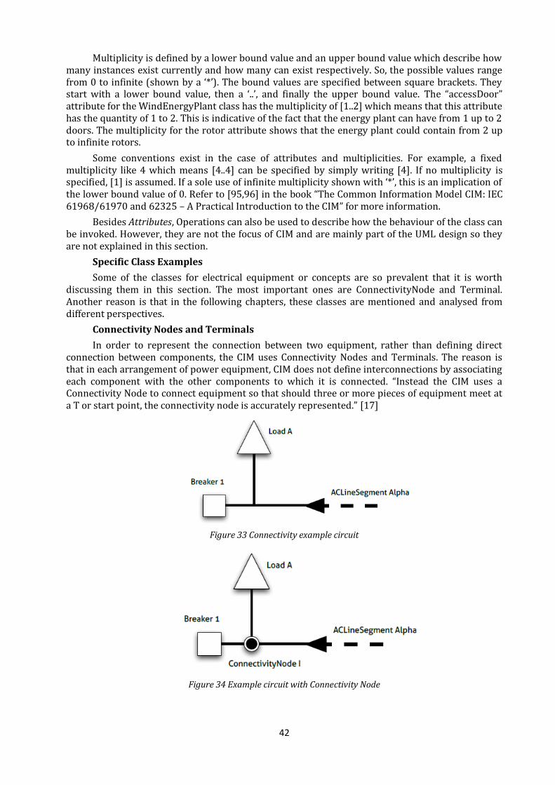
42
Multiplicity is defined by a lower bound value and an upper bound value which describe how many instances exist currently and how many can exist respectively. So, the possible values range from 0 to infinite (shown by a ‘*’). The bound values are specified between square brackets. They start with a lower bound value, then a ‘..’, and finally the upper bound value. The “accessDoor” attribute for the WindEnergyPlant class has the multiplicity of [1..2] which means that this attribute has the quantity of 1 to 2. This is indicative of the fact that the energy plant can have from 1 up to 2 doors. The multiplicity for the rotor attribute shows that the energy plant could contain from 2 up to infinite rotors.
Some conventions exist in the case of attributes and multiplicities. For example, a fixed multiplicity like 4 which means [4..4] can be specified by simply writing [4]. If no multiplicity is specified, [1] is assumed. If a sole use of infinite multiplicity shown with ‘*’, this is an implication of the lower bound value of 0. Refer to [95,96] in the book “The Common Information Model CIM: IEC 61968/61970 and 62325 – A Practical Introduction to the CIM” for more information.
Besides Attributes, Operations can also be used to describe how the behaviour of the class can be invoked. However, they are not the focus of CIM and are mainly part of the UML design so they are not explained in this section.
Specific Class Examples
Some of the classes for electrical equipment or concepts are so prevalent that it is worth discussing them in this section. The most important ones are ConnectivityNode and Terminal. Another reason is that in the following chapters, these classes are mentioned and analysed from different perspectives.
Connectivity Nodes and Terminals
In order to represent the connection between two equipment, rather than defining direct connection between components, the CIM uses Connectivity Nodes and Terminals. The reason is that in each arrangement of power equipment, CIM does not define interconnections by associating each component with the other components to which it is connected. “Instead the CIM uses a Connectivity Node to connect equipment so that should three or more pieces of equipment meet at a T or start point, the connectivity node is accurately represented.” [17]
Figure 33 Connectivity example circuit
Figure 34 Example circuit with Connectivity Node
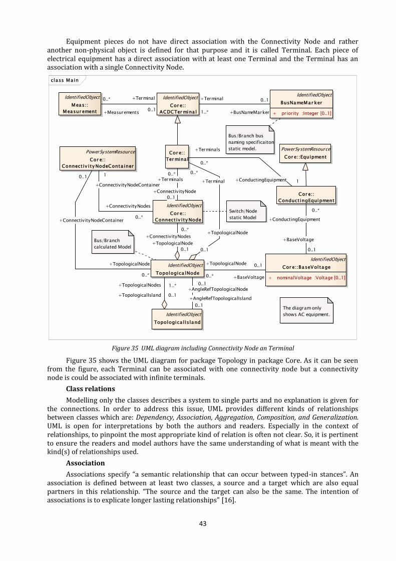
43
Equipment pieces do not have direct association with the Connectivity Node and rather another non-physical object is defined for that purpose and it is called Terminal. Each piece of electrical equipment has a direct association with at least one Terminal and the Terminal has an association with a single Connectivity Node.
Figure 35 UML diagram including Connectivity Node an Terminal
Figure 35 shows the UML diagram for package Topology in package Core. As it can be seen from the figure, each Terminal can be associated with one connectivity node but a connectivity node is could be associated with infinite terminals.
Class relations
Modelling only the classes describes a system to single parts and no explanation is given for the connections. In order to address this issue, UML provides different kinds of relationships between classes which are: Dependency, Association, Aggregation, Composition, and Generalization. UML is open for interpretations by both the authors and readers. Especially in the context of relationships, to pinpoint the most appropriate kind of relation is often not clear. So, it is pertinent to ensure the readers and model authors have the same understanding of what is meant with the kind(s) of relationships used.
Association
Associations specify “a semantic relationship that can occur between typed-in stances”. An association is defined between at least two classes, a source and a target which are also equal partners in this relationship. “The source and the target can also be the same. The intention of associations is to explicate longer lasting relationships” [16].
cla ss Ma in
Switch/Node
static Model
IdentifiedObject
Cor e::
Connect iv i ty Node
PowerSystemResource
Cor e::
Connect iv i ty NodeConta iner
Cor e::
Ter mina l
Bus/Branch
calculated Model
IdentifiedObject
Topologica lNode
IdentifiedObject
Meas::
Measur ement
Cor e::
Conduct ingEquipment
IdentifiedObject
Topologica l Island
IdentifiedObject
BusNameMar ker
+ priority :Integer [0..1]
PowerSystemResource
Cor e::Equipment
Bus/Branch bus
naming specificaiton
static model.
IdentifiedObject
Cor e::
ACDCTer mina l
IdentifiedObject
Cor e::BaseVoltage
+ nominalVoltage :Voltage [0..1]
The diagram only
shows AC equipment.
+TopologicalNode
0..*
+ConnectivityNodeContainer
0..1
+TopologicalNodes 1..*
+TopologicalIsland 0..1
+BaseVoltage
0..1
+ConductingEquipment
0..*
+Terminals
0..*
+ConductingEquipment 1+Terminal
0..*
+TopologicalNode
0..1
+ConnectivityNodes
0..*
+TopologicalNode
0..1
+TopologicalNode
0..* +BaseVoltage
0..1
+ConnectivityNodes
0..*
+ConnectivityNodeContainer
1+Terminals
0..*
+ConnectivityNode
0..1
+BusNameMarker
0..1+Terminal
1..*+Measurements
0..* +Terminal
0..1
+AngleRefTopologicalIsland
0..1
+AngleRefTopologicalNode0..1
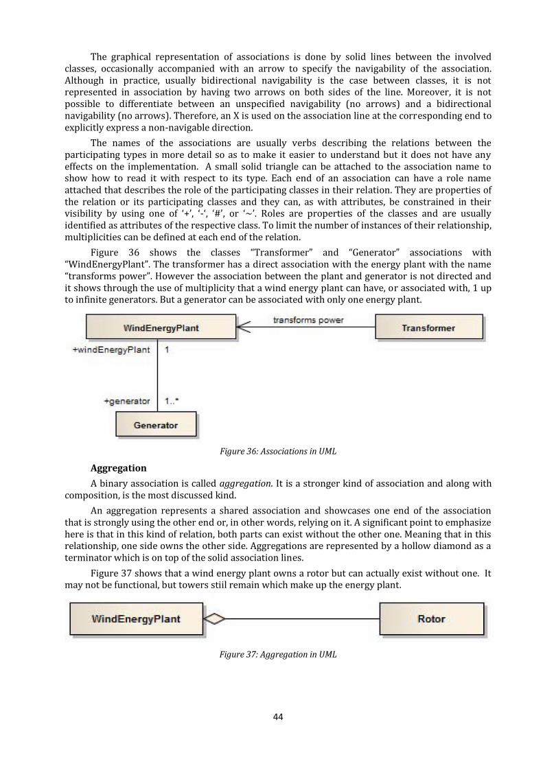
44
The graphical representation of associations is done by solid lines between the involved classes, occasionally accompanied with an arrow to specify the navigability of the association. Although in practice, usually bidirectional navigability is the case between classes, it is not represented in association by having two arrows on both sides of the line. Moreover, it is not possible to differentiate between an unspecified navigability (no arrows) and a bidirectional navigability (no arrows). Therefore, an X is used on the association line at the corresponding end to explicitly express a non-navigable direction.
The names of the associations are usually verbs describing the relations between the participating types in more detail so as to make it easier to understand but it does not have any effects on the implementation. A small solid triangle can be attached to the association name to show how to read it with respect to its type. Each end of an association can have a role name attached that describes the role of the participating classes in their relation. They are properties of the relation or its participating classes and they can, as with attributes, be constrained in their visibility by using one of ‘+’, ‘-‘, ‘#’, or ‘~’. Roles are properties of the classes and are usually identified as attributes of the respective class. To limit the number of instances of their relationship, multiplicities can be defined at each end of the relation.
Figure 36 shows the classes “Transformer” and “Generator” associations with “WindEnergyPlant”. The transformer has a direct association with the energy plant with the name “transforms power”. However the association between the plant and generator is not directed and it shows through the use of multiplicity that a wind energy plant can have, or associated with, 1 up to infinite generators. But a generator can be associated with only one energy plant.
Figure 36: Associations in UML
Aggregation
A binary association is called aggregation. It is a stronger kind of association and along with composition, is the most discussed kind.
An aggregation represents a shared association and showcases one end of the association that is strongly using the other end or, in other words, relying on it. A significant point to emphasize here is that in this kind of relation, both parts can exist without the other one. Meaning that in this relationship, one side owns the other side. Aggregations are represented by a hollow diamond as a terminator which is on top of the solid association lines.
Figure 37 shows that a wind energy plant owns a rotor but can actually exist without one. It may not be functional, but towers stiil remain which make up the energy plant.
Figure 37: Aggregation in UML
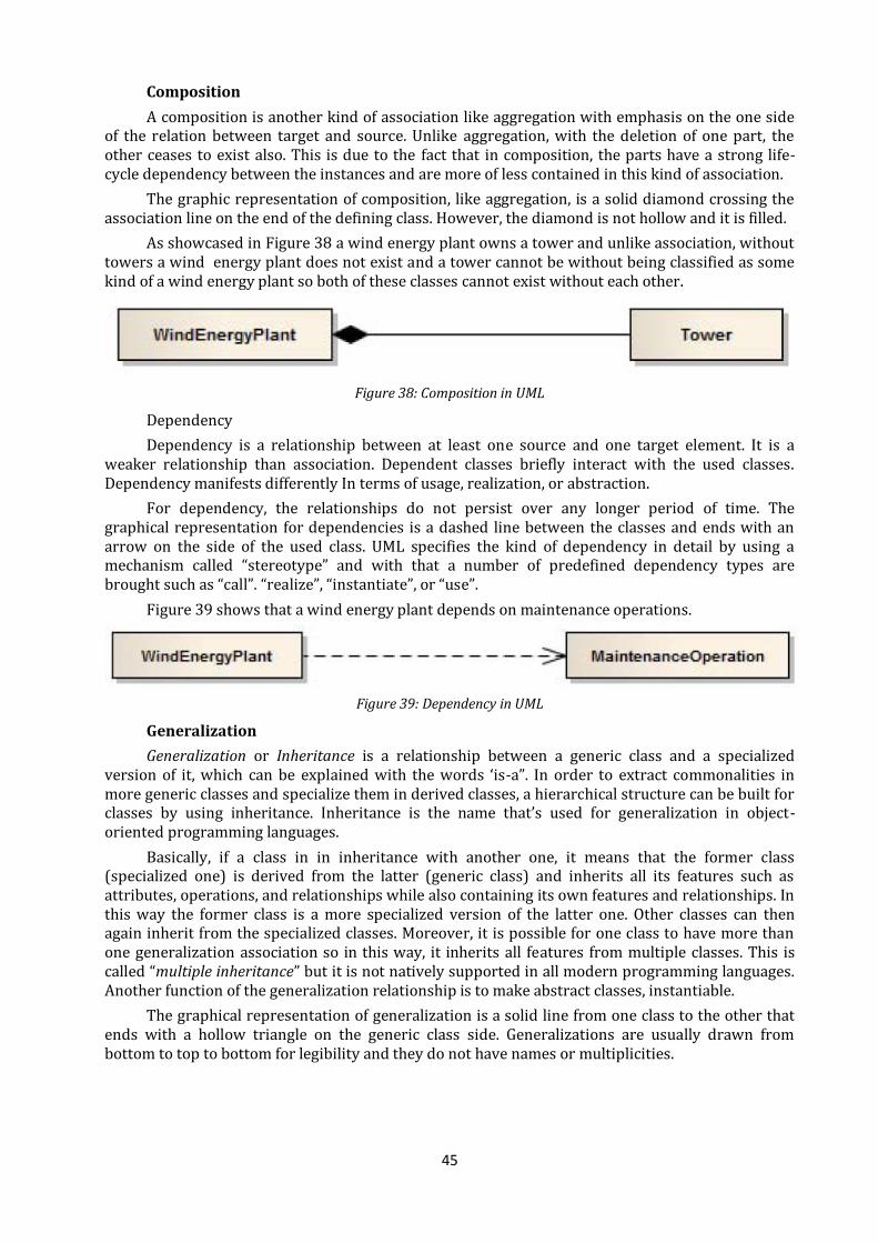
45
Composition
A composition is another kind of association like aggregation with emphasis on the one side of the relation between target and source. Unlike aggregation, with the deletion of one part, the other ceases to exist also. This is due to the fact that in composition, the parts have a strong life-cycle dependency between the instances and are more of less contained in this kind of association.
The graphic representation of composition, like aggregation, is a solid diamond crossing the association line on the end of the defining class. However, the diamond is not hollow and it is filled.
As showcased in Figure 38 a wind energy plant owns a tower and unlike association, without towers a wind energy plant does not exist and a tower cannot be without being classified as some kind of a wind energy plant so both of these classes cannot exist without each other.
Figure 38: Composition in UML
Dependency
Dependency is a relationship between at least one source and one target element. It is a weaker relationship than association. Dependent classes briefly interact with the used classes. Dependency manifests differently In terms of usage, realization, or abstraction.
For dependency, the relationships do not persist over any longer period of time. The graphical representation for dependencies is a dashed line between the classes and ends with an arrow on the side of the used class. UML specifies the kind of dependency in detail by using a mechanism called “stereotype” and with that a number of predefined dependency types are brought such as “call”. “realize”, “instantiate”, or “use”.
Figure 39 shows that a wind energy plant depends on maintenance operations.
Figure 39: Dependency in UML
Generalization
Generalization or Inheritance is a relationship between a generic class and a specialized version of it, which can be explained with the words ‘is-a”. In order to extract commonalities in more generic classes and specialize them in derived classes, a hierarchical structure can be built for classes by using inheritance. Inheritance is the name that’s used for generalization in object-oriented programming languages.
Basically, if a class in in inheritance with another one, it means that the former class (specialized one) is derived from the latter (generic class) and inherits all its features such as attributes, operations, and relationships while also containing its own features and relationships. In this way the former class is a more specialized version of the latter one. Other classes can then again inherit from the specialized classes. Moreover, it is possible for one class to have more than one generalization association so in this way, it inherits all features from multiple classes. This is called “multiple inheritance” but it is not natively supported in all modern programming languages. Another function of the generalization relationship is to make abstract classes, instantiable.
The graphical representation of generalization is a solid line from one class to the other that ends with a hollow triangle on the generic class side. Generalizations are usually drawn from bottom to top to bottom for legibility and they do not have names or multiplicities.
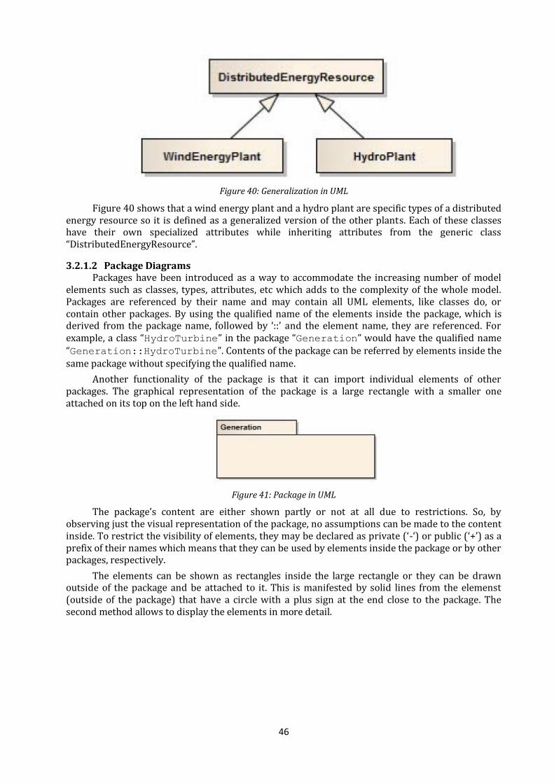
46
Figure 40: Generalization in UML
Figure 40 shows that a wind energy plant and a hydro plant are specific types of a distributed energy resource so it is defined as a generalized version of the other plants. Each of these classes have their own specialized attributes while inheriting attributes from the generic class “DistributedEnergyResource”.
3.2.1.2 Package Diagrams Packages have been introduced as a way to accommodate the increasing number of model
elements such as classes, types, attributes, etc which adds to the complexity of the whole model. Packages are referenced by their name and may contain all UML elements, like classes do, or contain other packages. By using the qualified name of the elements inside the package, which is derived from the package name, followed by ‘::’ and the element name, they are referenced. For example, a class “HydroTurbine” in the package “Generation” would have the qualified name “Generation::HydroTurbine”. Contents of the package can be referred by elements inside the same package without specifying the qualified name.
Another functionality of the package is that it can import individual elements of other packages. The graphical representation of the package is a large rectangle with a smaller one attached on its top on the left hand side.
Figure 41: Package in UML
The package’s content are either shown partly or not at all due to restrictions. So, by observing just the visual representation of the package, no assumptions can be made to the content inside. To restrict the visibility of elements, they may be declared as private (‘-‘) or public (‘+’) as a prefix of their names which means that they can be used by elements inside the package or by other packages, respectively.
The elements can be shown as rectangles inside the large rectangle or they can be drawn outside of the package and be attached to it. This is manifested by solid lines from the elemenst (outside of the package) that have a circle with a plus sign at the end close to the package. The second method allows to display the elements in more detail.
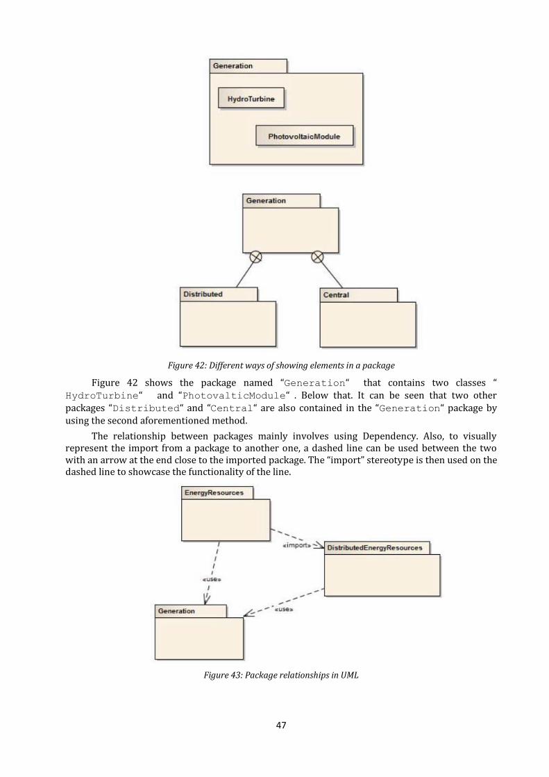
47
Figure 42: Different ways of showing elements in a package
Figure 42 shows the package named “Generation“ that contains two classes “ HydroTurbine“ and “PhotovalticModule“ . Below that. It can be seen that two other packages “Distributed“ and “Central“ are also contained in the “Generation“ package by using the second aforementioned method.
The relationship between packages mainly involves using Dependency. Also, to visually represent the import from a package to another one, a dashed line can be used between the two with an arrow at the end close to the imported package. The “import” stereotype is then used on the dashed line to showcase the functionality of the line.
Figure 43: Package relationships in UML
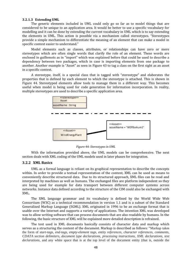
48
3.2.1.3 Extending UML The generic elements included in UML could only go so far as to model things that are
considered to be unique to an application area. It would be better to use a specific vocabulary for modelling and it can be done by extending the current vocabulary in UML which is to say extending the elements in UML. This action is possible via a mechanism called stereotypes. “Stereotypes provide a simple mechanism to differentiate the meaning of an element that can make a model in specific context easier to understand.”
Model elements such as classes, attributes, or relationships can have zero or more stereotypes which are often single words that clarify the role of an element. These words are enclosed in guillemots as in “import” which was explained before that could be used to describe a dependency between two packages, which in case is importing elements from one package to another. Another example is “Asset” as seen in Figure 43 to tag a class on the first sight as an asset in a specific context.
A stereotype, itself, is a special class that is tagged with “stereotype” and elaborates the properties that is defined by each element to which the stereotype is attached. This is shown in Figure 44. Stereotyped elements allow tools to manage them in a different way. This becomes useful when model is being used for code generation for information incorporation. In reality, multiple stereotypes are used to describe a specific application area.
Figure 44: Stereotypes in UML
With the information provided above, the UML models can be comprehensive. The next section deals with XML coding of the UML models used in later phases for integration.
3.2.2 XML Basics
UML as a formal language is reliant on its graphical representation to describe the concepts within. In order to provide a textual representation of the content, XML can be used as means to conveniently describe structured data. Due to its structured approach, XML files can be read and interpreted by machines as well as humans. The exchanged files are platform independent so they are being used for example for data transport between different computer systems across networks. Instance data defined according to the structure of the CIM could also be exchanged with XML.
The XML language grammar and its vocabulary is defined by the World Wide Web Consortium (W3C) as a technical recommendation in version 1.1 and is a subset of the Standard Generalized Markup Language (SGML). XML originated in 1996 to be an exchange format that is usable over the Internet and supports a variety of applications. The intention XML was developed was to allow writing software that can process documents that are also readable by humans. In the following, the basic structure of XML will be explained more detailed description is refrained.
The text used in XML documents basically consists of character data and markup which serves as a structuring the content of the document. Markup is described as follows: “Markup takes the form of start-tags, end-tags, empty-element tags, entity references, character references, comments,
CDATA section delimiters, document type declarations, processing instructions, XML declarations, text
declarations, and any white space that is at the top level of the document entity (that is, outside the

49
document element and not inside any other markup). These kinds of markup are defined between angle
brackets (< and >) and it is defined that those characters as well as the ampersand character (&) “must not
appear in their literal form, except when used as markup delimiters, or within a comment, a processing instruction, or a CDATA section”.1
3.2.2.1 Elements The XML can be logically structured with elements. Each document contains one or more
elements, all with names which are delimited by start-tag (<tag-name>) and end-tags (</tag-name>). The names of the start and end tags have to be exactly equal in case and can begin with a letter, colon, or underscore followed by different characters except space character that delimits the name. The use of colons or underscores at the beginning of a name is not recommended. Content can be placed between the tags which is comprised of character data, further elements, processing instructions, or comments.
<element>
Content
<emptyelement />
</element>
Attributes
Start-tags can have one or more attributes that define hey-value pairs. An attribute has a name (key) that has to be unique for an element. The name of the attribute is followed by an equal sign and the value is specified between two quotes. The attribute value can have any character data but does not contain any further tags. A space bracket is used to separate attributes from elements. The following example shows the usage of attributes in XML.
<element attributename="value">
Content
<emptyelement attributename="value1" anotherattribute="value2" />
</element>
3.2.2.2 Character Data and other Markup Elements All character are parsed and interpreted when used in XML. It also defines a way to use
special characters like angle brackets (<,>) that are normally disallowed or use Greek letter as content by reference.
“A character reference refers to a specific character in the ISO/IEC 10646 character set, for example one not directly accessible from available input devices. An entity refers to the content of a named entity.”2
References start with an ampersand symbol, followed by their identifier and end with a semi-colon. The identifier of character references starts with a hash symbol followed by the Unicode number (in decimal or hexadecimal notation) of the character to be shown (for example µ or
µ to refer to the Greek character ). An entity reference identifier is usually made of characters which are some inbuilt. Inbuilt entity references are:
• & for an ampersand symbol (&), • < for an left angle bracket (<), • > for an right angle bracket (>), • ' for an apostrophe (’) and
• " for an quotation mark (")
Character Data (CDATA) Sections
Another method to include specific character data without interpretation by the XML parser, are character data (CDATA) sections. They “occur anywhere character data may occur; they are used to escape blocks of text containing characters which would otherwise be recognized as
1 Insert reference (124) in CIM book
2 Insert reference
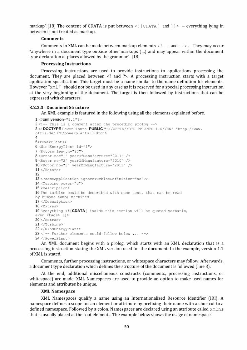
50
markup”.[18] The content of CDATA is put between <![CDATA[ and ]]> – everything lying in between is not treated as markup.
Comments
Comments in XML can be made between markup elements <!-- and -->. They may occur “anywhere in a document type outside other markups (…) and may appear within the document type declaration at places allowed by the grammar”. [18]
Processing Instructions
Processing instructions are used to provide instructions to applications processing the document. They are placed between <? and ?>. A processing instruction starts with a target application specification. This target must be a name similar to the name definition for elements. However “xml” should not be used in any case as it is reserved for a special processing instruction at the very beginning of the document. The target is then followed by instructions that can be expressed with characters.
3.2.2.3 Document Structure An XML example is featured in the following using all the elements explained before.
1 <?xml version="1.1"?>
2 <!-- This is a comment after the preceding prolog -->
3 <!DOCTYPE PowerPlants PUBLIC "-//OFFIS//DTD PPLANTS 1.0//EN" "http://www. offis.de/DTD/powerplants10.dtd">
4
5<PowerPlants>
6 <WindEnergyPlant id="1">
7 <Rotors length="20">
8 <Rotor no="1" yearOfManufacture="2011" />
9 <Rotor no="2" yearOfManufacture="2010" />
10 <Rotor no="3" yearOfManufacture="2011" />
11 </Rotors>
12
13 <?someApplication ignoreTurbineDefinition="no"?>
14 <Turbine power="3">
15 <Description>
16 The turbine could be described with some text, that can be read by humans & machines.
17 </Description>
18 <Extras>
19 Everything <![CDATA[ inside this section will be quoted verbatim, even <tags> ]]>
20 </Extras>
21 </Turbine>
22 </WindEnergyPlant>
23 <!-- Further elements could follow below ... -->
24 </PowerPlant>
An XML document begins with a prolog, which starts with an XML declaration that is a processing instruction stating the XML version used for the document. In the example, version 1.1 of XML is stated.
Comments, further processing instructions, or whitespace characters may follow. Afterwards, a document type declaration which defines the structure of the document is followed (line 3).
At the end, additional miscellaneous constructs (comments, processing instructions, or whitespace) are made. XML Namespaces are used to provide an option to make used names for elements and attributes be unique.
XML Namespace
XML Namespaces qualify a name using an Internationalized Resource Identifier (IRI). A namespace defines a scope for an element or attribute by prefixing their name with a shortcut to a defined namespace. Followed by a colon. Namespaces are declared using an attribute called xmlns that is usually placed at the root elements. The example below shows the usage of namespace.

51
1 <?xml version="1.1"?>
2 <PowerPlants xmlns="http://www.offis.de/pplants"
3 xmlns:cb="http://www.offis.de/cim-book">
4 <!--
5 The MicroCHP-element is in the default namespace http://www.offis.de/
pplants
6 The explanation-attribute’s namespace is http://www.offis.de/cim-book
7 -->
8 <MicroCHP id="2" cb:explanation="Combined Heat and Power">
9 <cb:example>
10 This example-element’s namespace is http://www.offis.de/cim-book
11 It is not part of the default namespace.
12 </cb:example>
13 <!-- ... -->
14 </MicroCHP>
15 </PowerPlant>
3.2.3 RDF Basics
XML is a well-structured technology that is readable by machines and understandable by humans. Although, one of its major shortcomings is that there is no link to what the tags in XML really mean except their name. Humans understand the tags since their name assumes a specific thing that is associated with it so it has a meaning to humans. RDF focuses on the description of resources and therefore addresses the lack of semantic in XML.
It is defined by a set of W3C recommendations and is intended to serve as a standard model for meta data interchange on the web. The approach it takes and the application it is intended for goes beyond just the syntactic description of data, as it is possible with XML and XML schema. “RDF provides features to semantically describe information and so to facilitate the integration of multiple information sources”. RDF provides a common framework so that the information could be exchanged without losing its meaning. The advantage is that it can be processed by machines while being understandable by humans. RDF in the context of CIM is used to serialize network topology data.
Essentially, RDF describes resources, identified by Uniform Resource Identifiers (URIs) and sets them in relation to their resources. This is realized using a triple made up of a subject, a predicate, and an object. The subject describes the resource about which a statement shall be expressed, the predicate refers to a certain property of an object and the object serves as an argument for the predicate. A graphical representation of this structure could be having the resources (subject and object) as nodes and the predicate as labelled edge. In an RDF graph, resources are symbolized by an ellipse and literals, representing data values, are symbolized by rectangles. The figure below shows an RDF graph.
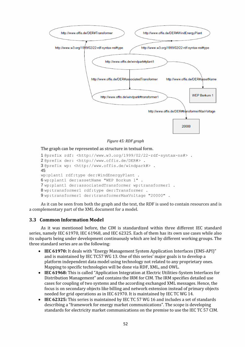
52
Figure 45: RDF graph
The graph can be represented as structure in textual form.
1 @prefix rdf: <http://www.w3.org/1999/02/22-rdf-syntax-ns#> .
2 @prefix der: <http://www.offis.de/DER#> .
3 @prefix wp: <http://www.offis.de/windpark#> .
45 wp:plant1 rdf:type der:WindEnergyPlant .
6 wp:plant1 der:assetName "WEP Borkum 1" .
7 wp:plant1 der:associatedTransformer wp:transformer1 .
8 wp:transformer1 rdf:type der:Transformer .
9 wp:transformer1 der:transformerMaxVoltage "20000" .
As it can be seen from both the graph and the text, the RDF is used to contain resources and is a complementary part of the XML document for a model.
3.3 Common Information Model
As it was mentioned before, the CIM is standardized within three different IEC standard series, namely IEC 61970, IEC 61968, and IEC 62325. Each of them has its own use cases while also its subparts being under development continuously which are led by different working groups. The three standard series are as the following:
IEC 61970: It deals with “Energy Management System Application Interfaces (EMS-API)” and is maintained by IEC TC57 WG 13. One of this series’ major goals is to develop a platform independent data model using technology not related to any proprietary ones. Mapping to specific technologies will be done via RDF, XML, and OWL.
IEC 61968: This is called “Application Integration at Electric Utilities-System Interfaces for Distribution Management” and contains the IRM for CIM. The IRM specifies detailed use cases for coupling of two systems and the according exchanged XML messages. Hence, the focus is on secondary objects like billing and network extension instead of primary objects needed for grid operations as in IEC 61970. It is maintained by IEC TC WG 14.
IEC 62325: This series is maintained by IEC TC 57 WG 16 and includes a set of standards describing a “framework for energy market communications”. The scope is developing standards for electricity market communications on the premise to use the IEC TC 57 CIM.
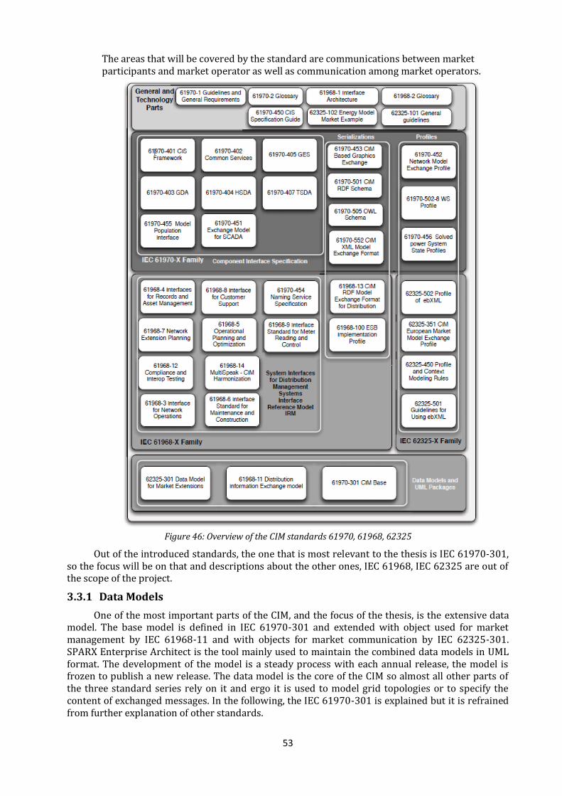
53
The areas that will be covered by the standard are communications between market participants and market operator as well as communication among market operators.
Figure 46: Overview of the CIM standards 61970, 61968, 62325
Out of the introduced standards, the one that is most relevant to the thesis is IEC 61970-301, so the focus will be on that and descriptions about the other ones, IEC 61968, IEC 62325 are out of the scope of the project.
3.3.1 Data Models
One of the most important parts of the CIM, and the focus of the thesis, is the extensive data model. The base model is defined in IEC 61970-301 and extended with object used for market management by IEC 61968-11 and with objects for market communication by IEC 62325-301. SPARX Enterprise Architect is the tool mainly used to maintain the combined data models in UML format. The development of the model is a steady process with each annual release, the model is frozen to publish a new release. The data model is the core of the CIM so almost all other parts of the three standard series rely on it and ergo it is used to model grid topologies or to specify the content of exchanged messages. In the following, the IEC 61970-301 is explained but it is refrained from further explanation of other standards.
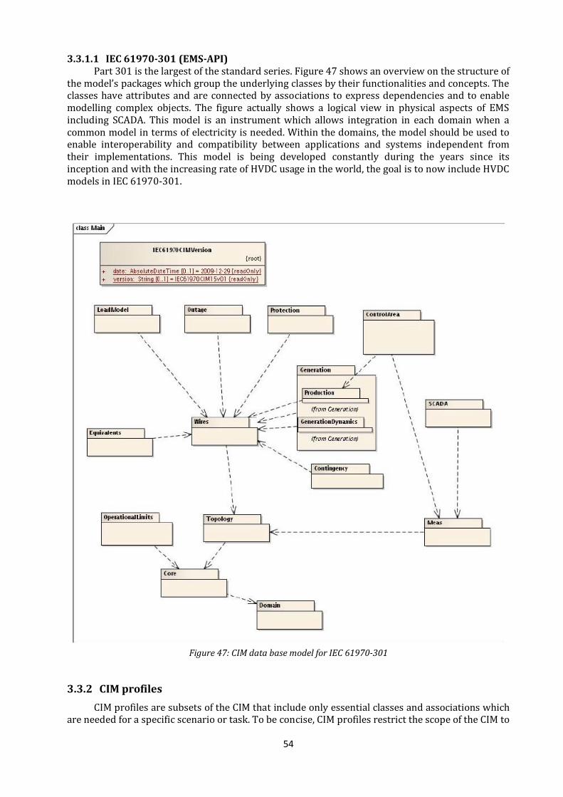
54
3.3.1.1 IEC 61970-301 (EMS-API) Part 301 is the largest of the standard series. Figure 47 shows an overview on the structure of
the model’s packages which group the underlying classes by their functionalities and concepts. The classes have attributes and are connected by associations to express dependencies and to enable modelling complex objects. The figure actually shows a logical view in physical aspects of EMS including SCADA. This model is an instrument which allows integration in each domain when a common model in terms of electricity is needed. Within the domains, the model should be used to enable interoperability and compatibility between applications and systems independent from their implementations. This model is being developed constantly during the years since its inception and with the increasing rate of HVDC usage in the world, the goal is to now include HVDC models in IEC 61970-301.
Figure 47: CIM data base model for IEC 61970-301
3.3.2 CIM profiles
CIM profiles are subsets of the CIM that include only essential classes and associations which are needed for a specific scenario or task. To be concise, CIM profiles restrict the scope of the CIM to

55
selected elements of the CIM like classes. Through CIM profiles, the use of CIM gets easier and more accessible. CIM profiles distinguish between mandatory and optional attributes and cardinalities of associations for given use cases. Therefore, interoperability tests (IOP) and conformity tests are performed against profiles. While standardized profiles exist within the utility domain, companies have their own intra-corporate profiles used for IOP tests within the company. The most common ones are as the following:
CPSM: The Common Power System Model (CPSM) is used in the USA for the exchange of transmission system models.
CDPSM: The Common Distribution Power System Model (CDPSM) is used in Europe for the exchange of distribution power system models.
ENTSO-E: The ENTSO-E profile is used in Europe for the exchange of transmission system models.
ERCOT: The Electric Reliability Council of Texas (ERCOT) profile is an intra-corporate data model.
56
4 CIM DC Load model
4.1 HVDC Power Flow model description
As discussed before, the main scope of the thesis is development of CIM load model and components for HVDC transmission systems. To develop the load model the power flow models of different HVDC substation topologies has to be researched.
Modelling HVDC systems typically have three levels of details:
simplified system model used in operations and planning. simplified system model supporting dynamic studies. detailed for transient studies of a HVDC station.
CIM load models of HVDC systems have 2 levels of details:
simplified load model used in power flow calculation detailed dynamic model for transient studies
In this thesis only the simplified power flow model of HVDC systems is under scope of research. Since the HVDC systems exist in 2 various topologies: Current source converter (CSC) and Voltage source converter(VSC), the similarity and individuality of CSC and VSC power flow models have to be discovered and described.
In order to provide the essential description of the simplified load model of HVDC systems in SCADA/EMS power flow models the following steps have to be taken:
The crucial components of HVDC systems in both topologies would have to be studied in scope of their individual functionality, role in the HVDC system, and impact on the power flow model. The list of electrical parameters of HVDC components taken into consideration in power flow calculation can be presented.
The crucial state variables and their relations relevant to power flow calculations would have to be presented. The similarity and individuality of essential formulas for both topologies have to be described.
The control modes and variables relevant to power flow model could be described. Since most of current HVDC technologies are recently developed, they are still under further development and belong to company’s proprietary information. Hence detailed description of control algorithms or internal variables in existing HVDC transmission systems can’t be presented.
Having studied the crucial component and relations in the HVDC transmission systems with CSC and VSC topologies and provided the list of essential system parameters, state and control variables relevant to power flow calculations, the presented simplified load model could be used for further implementation in HVDC CIM load model and validation the existing UML diagrams of DC CIM classes.
CSC Topology
Current source converter topology is still preferably used in existing HVDC transmission system in the world, even this topology doesn’t provide a good opportunity to development of DC grids. The main benefit of CSC is considerably lower cost and possibility of transferring high power. This topology is mainly applied in submarine and underground HVDC point-to point links.
As explained in section 2.12 the LCC CSC link doesn’t provide an opportunity for bidirectional power transfer. So most of existing HVDC LCC transmission system have bipolar configuration. A typical bipolar current source HVDC link is modelled as shown in Figure 48.
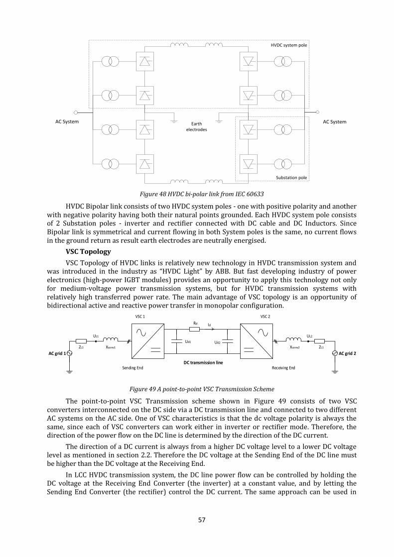
57
AC System
HVDC system pole
Substation pole
Earth electrodes
AC System
Figure 48 HVDC bi-polar link from IEC 60633
HVDC Bipolar link consists of two HVDC system poles - one with positive polarity and another with negative polarity having both their natural points grounded. Each HVDC system pole consists of 2 Substation poles - inverter and rectifier connected with DC cable and DC Inductors. Since Bipolar link is symmetrical and current flowing in both System poles is the same, no current flows in the ground return as result earth electrodes are neutrally energised.
VSC Topology
VSC Topology of HVDC links is relatively new technology in HVDC transmission system and was introduced in the industry as “HVDC Light” by ABB. But fast developing industry of power electronics (high-power IGBT modules) provides an opportunity to apply this technology not only for medium-voltage power transmission systems, but for HVDC transmission systems with relatively high transferred power rate. The main advantage of VSC topology is an opportunity of bidirectional active and reactive power transfer in monopolar configuration.
AC grid 1 AC grid 2
Sending End
ZL1 Xconv1
UL1
Receiving End
VSC 1 VSC 2
Ud1 Ud2
Rd Id
DC transmission line
Xconv2
UL2
ZL1
Figure 49 A point-to-point VSC Transmission Scheme
The point-to-point VSC Transmission scheme shown in Figure 49 consists of two VSC converters interconnected on the DC side via a DC transmission line and connected to two different AC systems on the AC side. One of VSC characteristics is that the dc voltage polarity is always the same, since each of VSC converters can work either in inverter or rectifier mode. Therefore, the direction of the power flow on the DC line is determined by the direction of the DC current.
The direction of a DC current is always from a higher DC voltage level to a lower DC voltage level as mentioned in section 2.2. Therefore the DC voltage at the Sending End of the DC line must be higher than the DC voltage at the Receiving End.
In LCC HVDC transmission system, the DC line power flow can be controlled by holding the DC voltage at the Receiving End Converter (the inverter) at a constant value, and by letting the Sending End Converter (the rectifier) control the DC current. The same approach can be used in
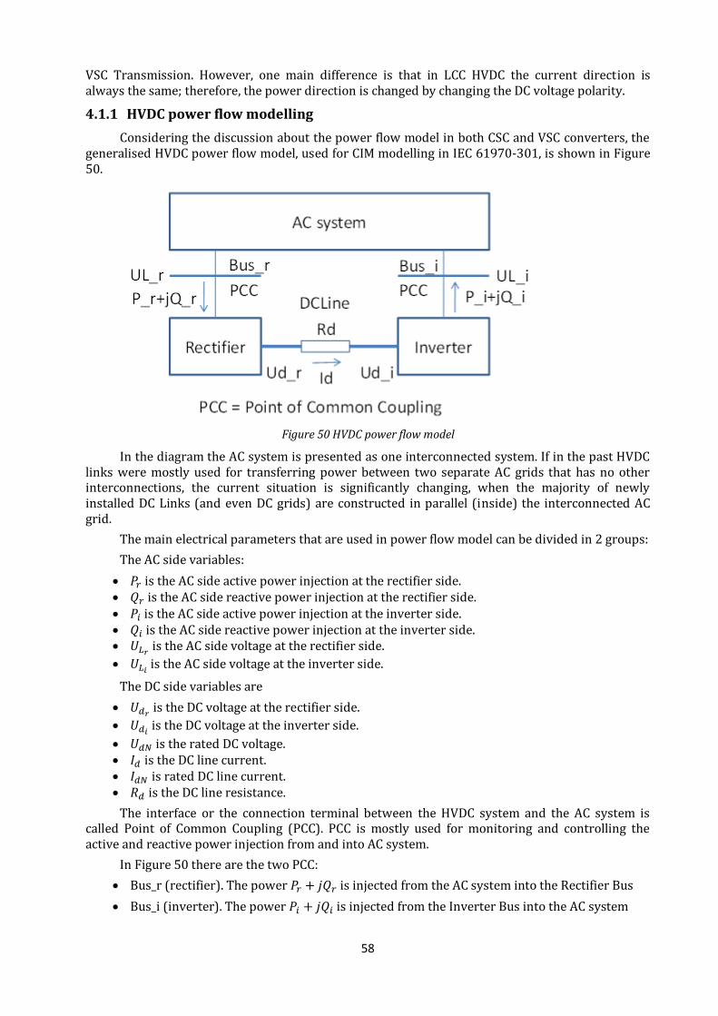
58
VSC Transmission. However, one main difference is that in LCC HVDC the current direction is always the same; therefore, the power direction is changed by changing the DC voltage polarity.
4.1.1 HVDC power flow modelling
Considering the discussion about the power flow model in both CSC and VSC converters, the generalised HVDC power flow model, used for CIM modelling in IEC 61970-301, is shown in Figure 50.
Figure 50 HVDC power flow model
In the diagram the AC system is presented as one interconnected system. If in the past HVDC links were mostly used for transferring power between two separate AC grids that has no other interconnections, the current situation is significantly changing, when the majority of newly installed DC Links (and even DC grids) are constructed in parallel (inside) the interconnected AC grid.
The main electrical parameters that are used in power flow model can be divided in 2 groups:
The AC side variables:
is the AC side active power injection at the rectifier side. is the AC side reactive power injection at the rectifier side. is the AC side active power injection at the inverter side. is the AC side reactive power injection at the inverter side.
is the AC side voltage at the rectifier side.
is the AC side voltage at the inverter side.
The DC side variables are
is the DC voltage at the rectifier side.
is the DC voltage at the inverter side.
is the rated DC voltage. is the DC line current. is rated DC line current. is the DC line resistance.
The interface or the connection terminal between the HVDC system and the AC system is called Point of Common Coupling (PCC). PCC is mostly used for monitoring and controlling the active and reactive power injection from and into AC system.
In Figure 50 there are the two PCC:
Bus_r (rectifier). The power is injected from the AC system into the Rectifier Bus
Bus_i (inverter). The power is injected from the Inverter Bus into the AC system
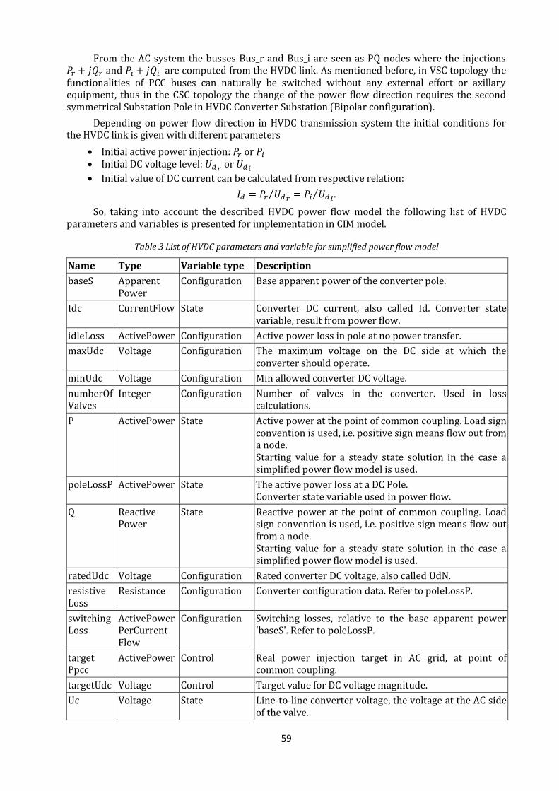
59
From the AC system the busses Bus_r and Bus_i are seen as PQ nodes where the injections and are computed from the HVDC link. As mentioned before, in VSC topology the functionalities of PCC buses can naturally be switched without any external effort or axillary equipment, thus in the CSC topology the change of the power flow direction requires the second symmetrical Substation Pole in HVDC Converter Substation (Bipolar configuration).
Depending on power flow direction in HVDC transmission system the initial conditions for the HVDC link is given with different parameters
Initial active power injection: or Initial DC voltage level: or
Initial value of DC current can be calculated from respective relation:
⁄
⁄ .
So, taking into account the described HVDC power flow model the following list of HVDC parameters and variables is presented for implementation in CIM model.
Table 3 List of HVDC parameters and variable for simplified power flow model
Name Type Variable type Description
baseS Apparent Power
Configuration Base apparent power of the converter pole.
Idc CurrentFlow State Converter DC current, also called Id. Converter state variable, result from power flow.
idleLoss ActivePower Configuration Active power loss in pole at no power transfer.
maxUdc Voltage Configuration The maximum voltage on the DC side at which the converter should operate.
minUdc Voltage Configuration Min allowed converter DC voltage.
numberOfValves
Integer Configuration Number of valves in the converter. Used in loss calculations.
P ActivePower State Active power at the point of common coupling. Load sign convention is used, i.e. positive sign means flow out from a node. Starting value for a steady state solution in the case a simplified power flow model is used.
poleLossP ActivePower State The active power loss at a DC Pole. Converter state variable used in power flow.
Q Reactive Power
State Reactive power at the point of common coupling. Load sign convention is used, i.e. positive sign means flow out from a node. Starting value for a steady state solution in the case a simplified power flow model is used.
ratedUdc Voltage Configuration Rated converter DC voltage, also called UdN.
resistive Loss
Resistance Configuration Converter configuration data. Refer to poleLossP.
switchingLoss
ActivePower PerCurrent Flow
Configuration Switching losses, relative to the base apparent power 'baseS'. Refer to poleLossP.
target Ppcc
ActivePower Control Real power injection target in AC grid, at point of common coupling.
targetUdc Voltage Control Target value for DC voltage magnitude.
Uc Voltage State Line-to-line converter voltage, the voltage at the AC side of the valve.
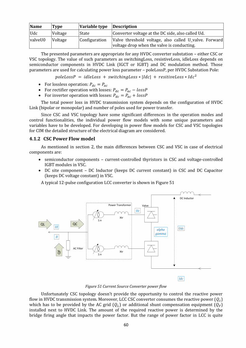
60
Name Type Variable type Description
Udc Voltage State Converter voltage at the DC side, also called Ud.
valveU0 Voltage Configuration Valve threshold voltage, also called U_valve. Forward voltage drop when the valve is conducting.
The presented parameters are appropriate for any HVDC converter substation – either CSC or VSC topology. The value of such parameters as switchingLoss, resistiveLoss, idleLoss depends on semiconductor components in HVDC Link (IGCT or IGBT) and DC modulation method. Those parameters are used for calculating power loss parameter – poleLossP, per HVDC Substation Pole:
For lossless operation: For rectifier operation with losses: For inverter operation with losses:
The total power loss in HVDC transmission system depends on the configuration of HVDC Link (bipolar or monopolar) and number of poles used for power transfer.
Since CSC and VSC topology have some significant differences in the operation modes and control functionalities, the individual power flow models with some unique parameters and variables have to be developed. For developing in power flow models for CSC and VSC topologies for CIM the detailed structure of the electrical diagram are considered.
4.1.2 CSC Power Flow model
As mentioned in section 2, the main differences between CSC and VSC in case of electrical components are:
semiconductor components – current-controlled thyristors in CSC and voltage-controlled IGBT modules in VSC.
DC site component – DC Inductor (keeps DC current constant) in CSC and DC Capacitor (keeps DC voltage constant) in VSC.
A typical 12-pulse configuration LCC converter is shown in Figure 51
Power Transformer
AC Filter
Valve
Uc
Idc
UdcUl
DC Inductor
alphagamma
Xtr
Xtr
1:n
1:n
Il
QL
QF
QC
Figure 51 Current Source Converter power flow
Unfortunately CSC topology doesn’t provide the opportunity to control the reactive power flow in HVDC transmission system. Moreover, LCC CSC converter consumes the reactive power ( ) which has to be provided by the AC grid ( ) or additional shunt compensation equipment ( ) installed next to HVDC Link. The amount of the required reactive power is determined by the bridge firing angle that impacts the power factor. But the range of power factor in LCC is quite
61
small, so the approximate reactive power injected in the converter is 50-60 % of transferred active power.
The amount of active power injected in the HVDC Link is controlled by the firing angle as well. A typical value of the firing angle is between 10 and 18 degrees.
The value of the DC voltage is defined by the following expression [11]
(
) (
)
where the rated direct voltage is calculated as:
√ ⁄
– the voltage level in the AC grid.
Installation of the additional shunt compensation equipment to compensate the reactive power consumption increases the cost of the HVDC transmission system, but in most cases the existing AC grid connected to HVDC link can’t provide the required reactive power. The approximation of reactive power injection could be presented in the following way:
(
)
where – the reactive power injected from the AC grid; - the reactive power compensated with AC Filter installed in HVDC Substation and proportional to required injected reactive power .
So, having researched the presented CSC power flow model the following parameters and variables for CIM modelling are proposed:
Table 4 List of CSC parameters and variables for simplified power flow model
Name Type Variable type Description
alpha AngleDegrees State Firing angle, typical value between 10 and 18 degrees for a rectifier.
gamma AngleDegrees State Extinction angle
maxAlpha AngleDegrees Configuration Maximum firing angle
maxGamma AngleDegrees Configuration Maximum extinction angle
maxIdc CurrentFlow Configuration The maximum direct current (Id) on the DC side at which the converter should operate.
minAlpha AngleDegrees Configuration Minimum firing angle
minGamma AngleDegrees Configuration Minimum extinction angle
minIdc CurrentFlow Configuration The minimum direct current (Id) on the DC side at which the converter should operate.
Operating Mode
CsOperating ModeKind
Control Indicates whether the DC pole is operating as an inverter or as a rectifier.
pPccControl CsPpcc ControlKind
Control Control mode of Active Power Control. It defines the reference parameter used in Active Power Control.
ratedIdc CurrentFlow Configuration Rated converter DC current, also called IdN.
targetAlpha AngleDegrees Control Target firing angle
targetGamma AngleDegrees Control Target extinction angle
targetIdc CurrentFlow Control DC current target value
Depending on the operationMode (inverter, rectifier) either firing or extinction angle control is crucial in active power control. Configuration parameters maxAlpha, minAlpha and control
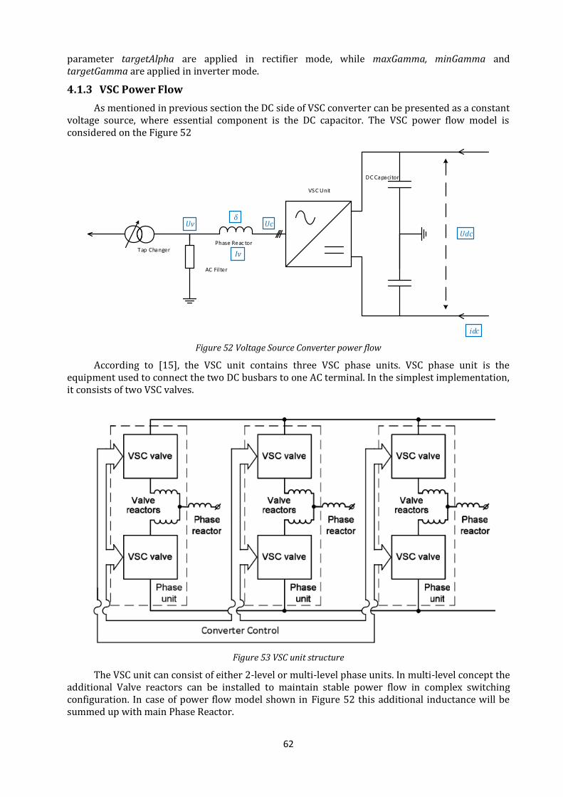
62
parameter targetAlpha are applied in rectifier mode, while maxGamma, minGamma and targetGamma are applied in inverter mode.
4.1.3 VSC Power Flow
As mentioned in previous section the DC side of VSC converter can be presented as a constant voltage source, where essential component is the DC capacitor. The VSC power flow model is considered on the Figure 52
AC Filter
Phase Reac torTap Changer
VSC Unit
Uc
idc
Udc
Uvδ
DC Capacitor
Iv
Figure 52 Voltage Source Converter power flow
According to [15], the VSC unit contains three VSC phase units. VSC phase unit is the equipment used to connect the two DC busbars to one AC terminal. In the simplest implementation, it consists of two VSC valves.
Figure 53 VSC unit structure
The VSC unit can consist of either 2-level or multi-level phase units. In multi-level concept the additional Valve reactors can be installed to maintain stable power flow in complex switching configuration. In case of power flow model shown in Figure 52 this additional inductance will be summed up with main Phase Reactor.
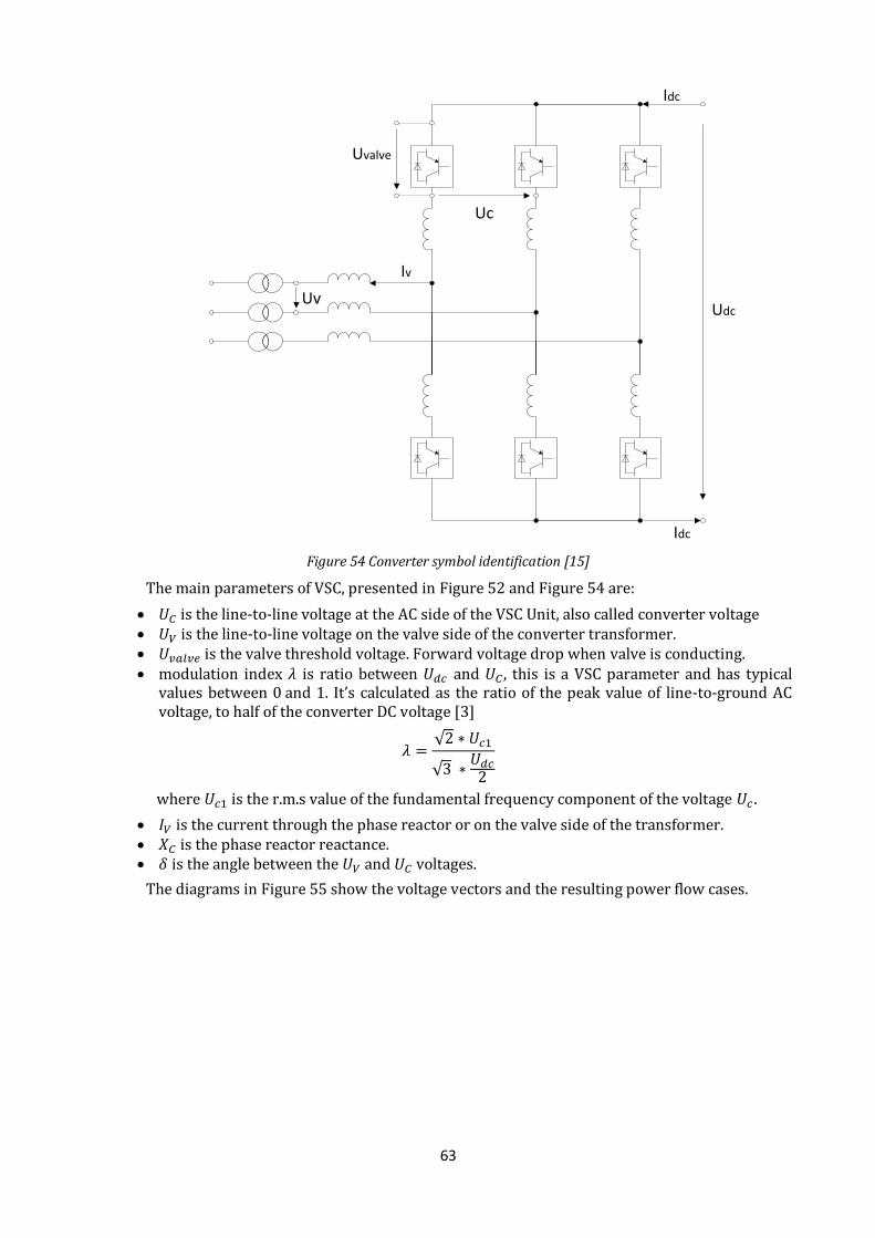
63
Uvalve
Uc
Uv
Iv
Idc
Idc
Udc
Figure 54 Converter symbol identification [15]
The main parameters of VSC, presented in Figure 52 and Figure 54 are:
is the line-to-line voltage at the AC side of the VSC Unit, also called converter voltage is the line-to-line voltage on the valve side of the converter transformer. is the valve threshold voltage. Forward voltage drop when valve is conducting. modulation index is ratio between and , this is a VSC parameter and has typical
values between and . It’s calculated as the ratio of the peak value of line-to-ground AC voltage, to half of the converter DC voltage [3]
√
√
where is the r.m.s value of the fundamental frequency component of the voltage .
is the current through the phase reactor or on the valve side of the transformer. is the phase reactor reactance. is the angle between the and voltages.
The diagrams in Figure 55 show the voltage vectors and the resulting power flow cases.
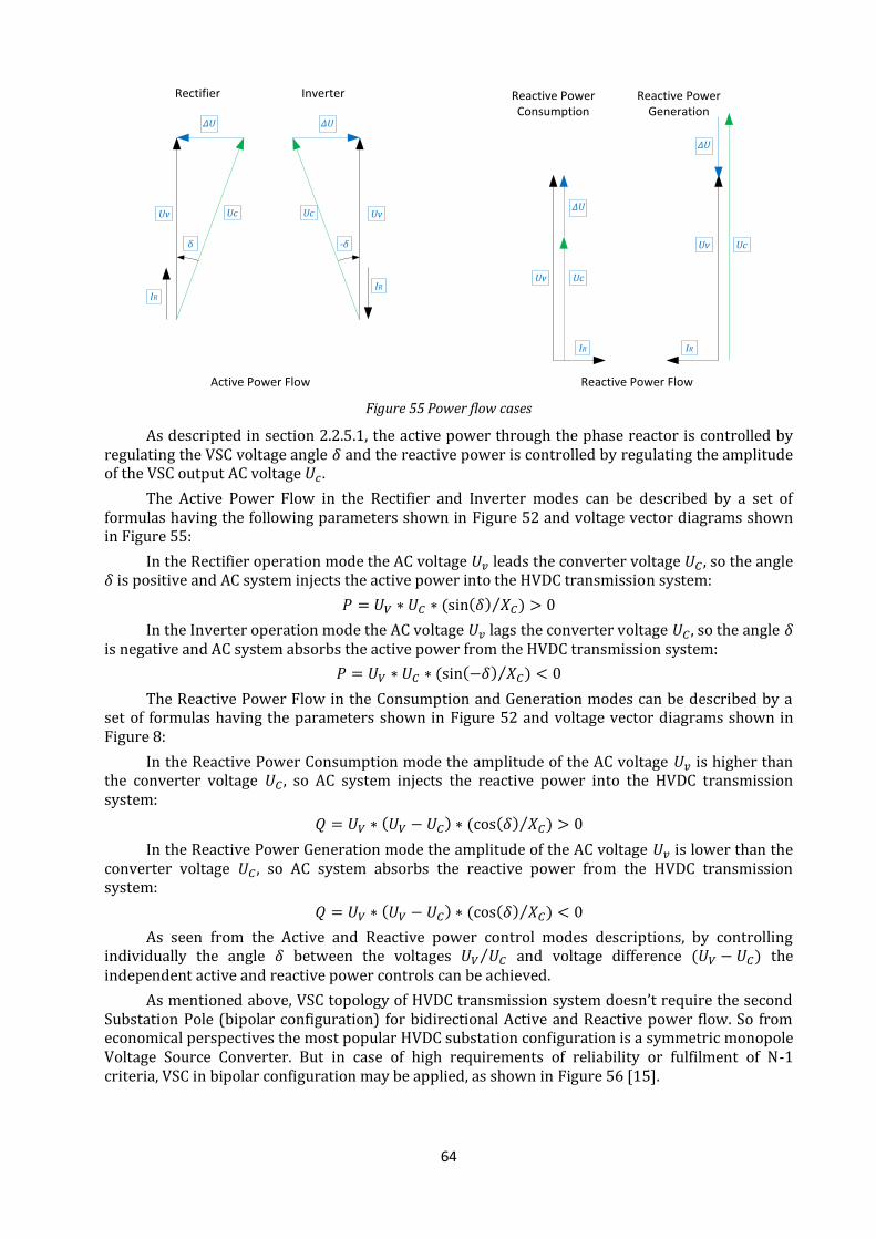
64
Uv Uc
δ
Uc Uv
-δ
IR
IR
ΔU ΔU
Uv
Uv Uc
Uc
ΔU
ΔU
IR IR
Rectifier Inverter Reactive Power Consumption
Reactive Power Generation
Active Power Flow Reactive Power Flow Figure 55 Power flow cases
As descripted in section 2.2.5.1, the active power through the phase reactor is controlled by regulating the VSC voltage angle and the reactive power is controlled by regulating the amplitude of the VSC output AC voltage .
The Active Power Flow in the Rectifier and Inverter modes can be described by a set of formulas having the following parameters shown in Figure 52 and voltage vector diagrams shown in Figure 55:
In the Rectifier operation mode the AC voltage leads the converter voltage , so the angle is positive and AC system injects the active power into the HVDC transmission system:
⁄
In the Inverter operation mode the AC voltage lags the converter voltage , so the angle is negative and AC system absorbs the active power from the HVDC transmission system:
⁄
The Reactive Power Flow in the Consumption and Generation modes can be described by a set of formulas having the parameters shown in Figure 52 and voltage vector diagrams shown in Figure 8:
In the Reactive Power Consumption mode the amplitude of the AC voltage is higher than the converter voltage , so AC system injects the reactive power into the HVDC transmission system:
⁄
In the Reactive Power Generation mode the amplitude of the AC voltage is lower than the converter voltage , so AC system absorbs the reactive power from the HVDC transmission system:
⁄
As seen from the Active and Reactive power control modes descriptions, by controlling individually the angle between the voltages ⁄ and voltage difference the independent active and reactive power controls can be achieved.
As mentioned above, VSC topology of HVDC transmission system doesn’t require the second Substation Pole (bipolar configuration) for bidirectional Active and Reactive power flow. So from economical perspectives the most popular HVDC substation configuration is a symmetric monopole Voltage Source Converter. But in case of high requirements of reliability or fulfilment of N-1 criteria, VSC in bipolar configuration may be applied, as shown in Figure 56 [15].
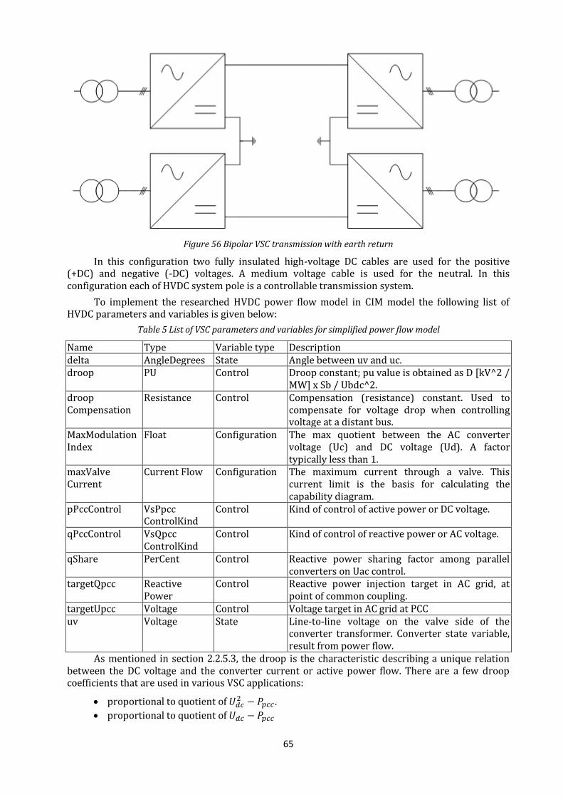
65
Figure 56 Bipolar VSC transmission with earth return
In this configuration two fully insulated high-voltage DC cables are used for the positive (+DC) and negative (-DC) voltages. A medium voltage cable is used for the neutral. In this configuration each of HVDC system pole is a controllable transmission system.
To implement the researched HVDC power flow model in CIM model the following list of HVDC parameters and variables is given below:
Table 5 List of VSC parameters and variables for simplified power flow model
Name Type Variable type Description delta AngleDegrees State Angle between uv and uc. droop PU Control Droop constant; pu value is obtained as D [kV^2 /
MW] x Sb / Ubdc^2. droop Compensation
Resistance Control Compensation (resistance) constant. Used to compensate for voltage drop when controlling voltage at a distant bus.
MaxModulation Index
Float Configuration The max quotient between the AC converter voltage (Uc) and DC voltage (Ud). A factor typically less than 1.
maxValve Current
Current Flow Configuration The maximum current through a valve. This current limit is the basis for calculating the capability diagram.
pPccControl VsPpcc ControlKind
Control Kind of control of active power or DC voltage.
qPccControl VsQpcc ControlKind
Control Kind of control of reactive power or AC voltage.
qShare PerCent Control Reactive power sharing factor among parallel converters on Uac control.
targetQpcc Reactive Power
Control Reactive power injection target in AC grid, at point of common coupling.
targetUpcc Voltage Control Voltage target in AC grid at PCC uv Voltage State Line-to-line voltage on the valve side of the
converter transformer. Converter state variable, result from power flow.
As mentioned in section 2.2.5.3, the droop is the characteristic describing a unique relation between the DC voltage and the converter current or active power flow. There are a few droop coefficients that are used in various VSC applications:
proportional to quotient of .
proportional to quotient of
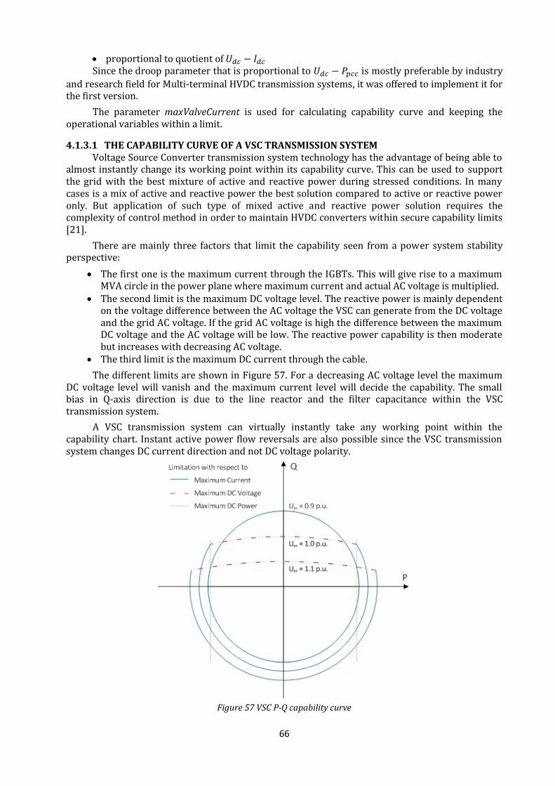
66
proportional to quotient of Since the droop parameter that is proportional to is mostly preferable by industry
and research field for Multi-terminal HVDC transmission systems, it was offered to implement it for the first version.
The parameter maxValveCurrent is used for calculating capability curve and keeping the operational variables within a limit.
4.1.3.1 THE CAPABILITY CURVE OF A VSC TRANSMISSION SYSTEM Voltage Source Converter transmission system technology has the advantage of being able to
almost instantly change its working point within its capability curve. This can be used to support the grid with the best mixture of active and reactive power during stressed conditions. In many cases is a mix of active and reactive power the best solution compared to active or reactive power only. But application of such type of mixed active and reactive power solution requires the complexity of control method in order to maintain HVDC converters within secure capability limits [21].
There are mainly three factors that limit the capability seen from a power system stability perspective:
The first one is the maximum current through the IGBTs. This will give rise to a maximum MVA circle in the power plane where maximum current and actual AC voltage is multiplied.
The second limit is the maximum DC voltage level. The reactive power is mainly dependent on the voltage difference between the AC voltage the VSC can generate from the DC voltage and the grid AC voltage. If the grid AC voltage is high the difference between the maximum DC voltage and the AC voltage will be low. The reactive power capability is then moderate but increases with decreasing AC voltage.
The third limit is the maximum DC current through the cable.
The different limits are shown in Figure 57. For a decreasing AC voltage level the maximum DC voltage level will vanish and the maximum current level will decide the capability. The small bias in Q-axis direction is due to the line reactor and the filter capacitance within the VSC transmission system.
A VSC transmission system can virtually instantly take any working point within the capability chart. Instant active power flow reversals are also possible since the VSC transmission system changes DC current direction and not DC voltage polarity.
Figure 57 VSC P-Q capability curve
67
4.2 CIM Data Model
4.2.1 CIM Component Structure
In order to create a suitable UML topology for HVDC components to be used in CIM the following steps have to be taken:
1. The HVDC components would have to be studied as efficiently as possible so that their individual functionality, relevance in the HVDC system, and their relationship to other HVDC equipment can be fully realized. The relevance is related to a certain subject used in simulations and further system analysis. For 61970-301, power flow is that subject.
2. Based on the knowledge gained from the first step, different HVDC components and equipment can be realized as CIM packages. Some packages can be analogous to an AC CIM package depending on the level of similarity that the particular HVDC component has to an AC one. And some packages can be created to suit the definition of the HVDC equipment and to fit within a bigger HVDC CIM package. Of course, from packages, classes are developed and also their respective relationship with each other.
3. Finally, once the CIM model has been created to a significant state, then it can be implemented to an Enterprise Architect scheme to be used later for analysis in different applications such as Network Manager.
It should be noted that since the HVDC implementation to CIM is rather new and HVDC converters have existed for a long time prior to CIM, the initial data models were created to suit an existing HVDC system so that information could be exchanged between that system and other ones or for study purposes. So, some aspects of the data model were quite specific. Since then, it has been changed to fit a more general structure. However, parts of it have not been fully included in UML yet due to their rather contemporary nature and being part of a company’s proprietary information, such as the control model.
One of the tasks of the thesis was to validate the already existing model of HVDC in Enterprise Architect based on the gained information about HVDC systems. Another was to convert it to the IEC 61970-301 document using JCleanCIM which will be discussed thoroughly later.
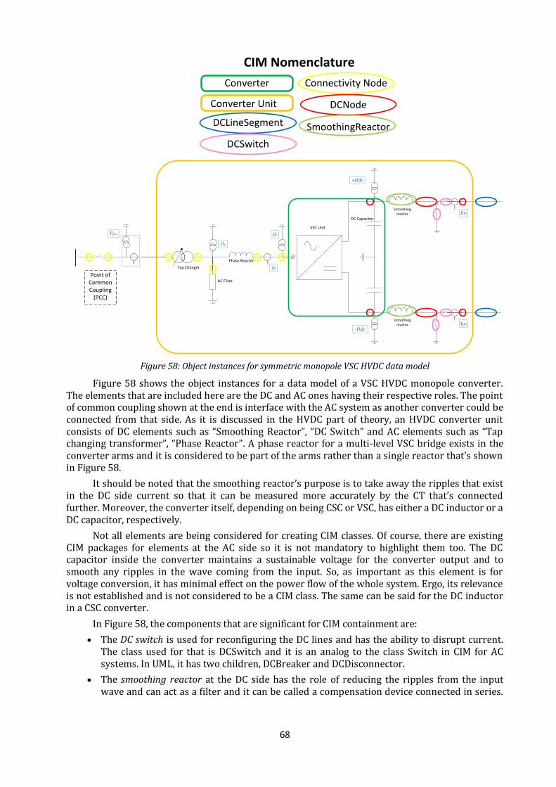
68
AC Filter
Phase Reactor
Tap Changer
VSC Unit
Uc
+Udc
Uv
DC Capacitor
IR
Smoothing reactor
-Udc
Smoothing reactor
IDC
IDC
Ppcc
Point of Common Coupling
(PCC)
DCNodeConverter Unit
CIM Nomenclature
Converter
DCLineSegment SmoothingReactor
Connectivity Node
DCSwitch
Figure 58: Object instances for symmetric monopole VSC HVDC data model
Figure 58 shows the object instances for a data model of a VSC HVDC monopole converter. The elements that are included here are the DC and AC ones having their respective roles. The point of common coupling shown at the end is interface with the AC system as another converter could be connected from that side. As it is discussed in the HVDC part of theory, an HVDC converter unit consists of DC elements such as “Smoothing Reactor”, “DC Switch” and AC elements such as “Tap changing transformer”, “Phase Reactor”. A phase reactor for a multi-level VSC bridge exists in the converter arms and it is considered to be part of the arms rather than a single reactor that’s shown in Figure 58.
It should be noted that the smoothing reactor’s purpose is to take away the ripples that exist in the DC side current so that it can be measured more accurately by the CT that’s connected further. Moreover, the converter itself, depending on being CSC or VSC, has either a DC inductor or a DC capacitor, respectively.
Not all elements are being considered for creating CIM classes. Of course, there are existing CIM packages for elements at the AC side so it is not mandatory to highlight them too. The DC capacitor inside the converter maintains a sustainable voltage for the converter output and to smooth any ripples in the wave coming from the input. So, as important as this element is for voltage conversion, it has minimal effect on the power flow of the whole system. Ergo, its relevance is not established and is not considered to be a CIM class. The same can be said for the DC inductor in a CSC converter.
In Figure 58, the components that are significant for CIM containment are:
The DC switch is used for reconfiguring the DC lines and has the ability to disrupt current. The class used for that is DCSwitch and it is an analog to the class Switch in CIM for AC systems. In UML, it has two children, DCBreaker and DCDisconnector.
The smoothing reactor at the DC side has the role of reducing the ripples from the input wave and can act as a filter and it can be called a compensation device connected in series.
69
So, the CIM class created for it is called DCSeriesDevice which is an analog to SeriesCompensation in AC systems.
Another concept that is essential in modelling for CIM is the connection points of equipment to each other. As it was said in chapter 1(theory, CIM section), this point is called the connectivity node and is used for gathering data such as current, voltage and power across equipment and interesting points in the topology. Connectivity node is the name for the AC CIM class so it wouldn’t go amiss if a name similar to that is used for the analogous DC concept. Also, reusing ConnectivityNode and Terminal for DC grids instigates mixing DC and AC components which is an error. Attributes have different meanings in AC and DC grids for example, there is no phase angle or reactive power injection in DC in this context. Ergo, DCNode (DCConnectivity Node previously) is used to describe points of connection between DC equipment and it is highlighted in the figure. The name of the CIM class is the same as DCNode. There is a DC analogue to the class Terminal as well but it is more complicated to describe than the DCNode and it will be explained in the later sections.
As described in the theory section, ACLineSegment is: “A wire or combination of wires, with consistent electrical characteristics, building a single electrical system, used to carry alternating current between points in the power system.”[16] The same premise can be used to define DCLineSegment, albeit cables are used mainly for transfer of power in HVDC systems, as it is highlighted in the figure and a CIM class has been named after it.
The converter that is shown in the figure consists of a VSC unit which is basically an IGBT PWM DC to AC converter. Its topology, function, and design have been elaborated in the theoretical section of the report. Other than the unit, DC capacitors are also part of the converter as they provide a smooth and stable voltage for the PWM Bridge. They are integral to the performance of the converter as a whole unit so they should be considered as part of the converter. Hence, the converter is significant per point of view of CIM and “ACDCConverter” is the corresponding CIM class in the UML that is used for load flow or other prospects. The converter is Figure 58 is VSC which is rather new. But, Line Commutating Converters or Current Source Converters as they are called have been used heavily in the past and are part of the foundation of HVDC systems. So the CIM class ACDCConverter has two children classes: VSCConverter and CSCConverter. They both inherit attributes from the parent class and have their own unique attributes as well. The old CIM RectifierInverter is identical with the Converter.
The converter, DC node, smoothing reactor, DC switch, and other components on the DC side along with the phase reactor, transformer on the AC side can be considered as a single converter unit which can be used in load flow calculations at a larger scale. Analysis of a power system as a whole is possible if the AC and DC substations are considered to be single units with their own measurements. Ergo, the collective of AC and DC equipment along with the converter is significant on its own and is called “Converter Unit” in Figure 58 and a CIM class “DCConverterUnit” has been made for that purpose. The DCConverterUnit in CIM is identical with IEC 60633 Substation Pole that is a container. The IEC 60633 System Pole is not modeled in CIM. Reason is the IEC 60633 System Pole is not relevant in DC grids.
With the existence of DCConverterUnit, the transformers are not part of the Substation anymore as they were in the CIM for AC systems. Moreover, there are no VoltageLevels (the CIM class) at the low and high voltage sides of the transformer since the containment rules for them no longer exist in this context and have been replaced by rules specific to the DCConverterUnit.
In Figure 58, a symmetric monopole configuration of a DC link is shown. In general, HVDC link can be operated in the following three ways:
1. Bipolar; 2. Symmetrical monopole with capacitive earthing on the d.c. side; 3. Asymmetrical monopole with ground return, this lower active power capacity and
sustained operation is not allowed;
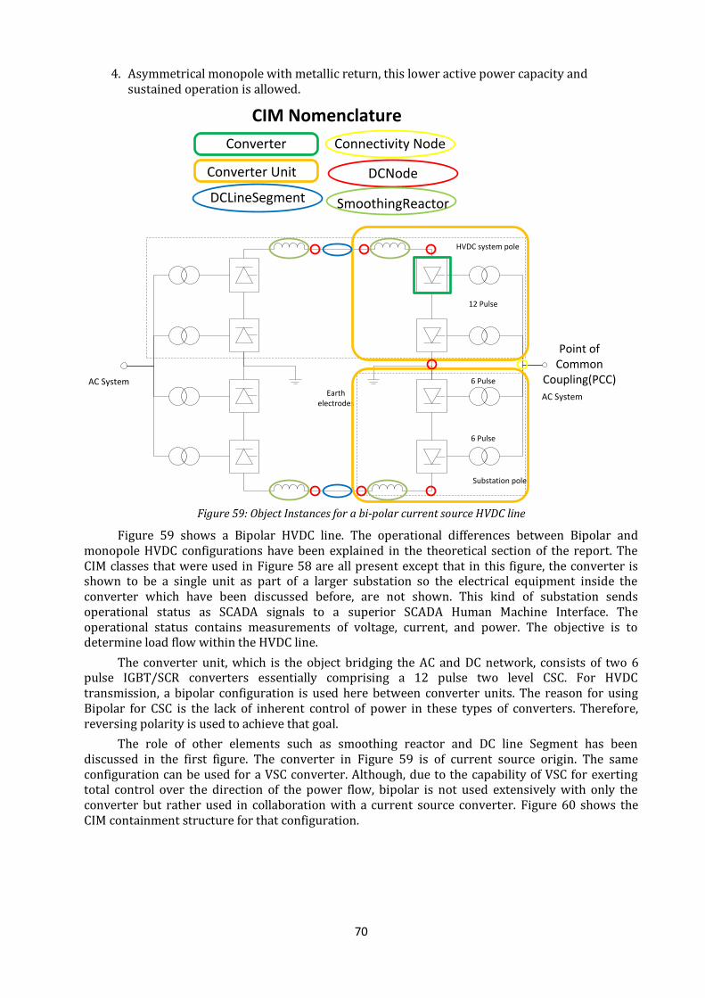
70
4. Asymmetrical monopole with metallic return, this lower active power capacity and sustained operation is allowed.
AC System
HVDC system pole
Substation pole
Earth electrodes
AC System
DCNodeConverter Unit
CIM Nomenclature
Converter
DCLineSegment SmoothingReactor
12 Pulse
6 Pulse
6 Pulse
Connectivity Node
Point of Common
Coupling(PCC)
Figure 59: Object Instances for a bi-polar current source HVDC line
Figure 59 shows a Bipolar HVDC line. The operational differences between Bipolar and monopole HVDC configurations have been explained in the theoretical section of the report. The CIM classes that were used in Figure 58 are all present except that in this figure, the converter is shown to be a single unit as part of a larger substation so the electrical equipment inside the converter which have been discussed before, are not shown. This kind of substation sends operational status as SCADA signals to a superior SCADA Human Machine Interface. The operational status contains measurements of voltage, current, and power. The objective is to determine load flow within the HVDC line.
The converter unit, which is the object bridging the AC and DC network, consists of two 6 pulse IGBT/SCR converters essentially comprising a 12 pulse two level CSC. For HVDC transmission, a bipolar configuration is used here between converter units. The reason for using Bipolar for CSC is the lack of inherent control of power in these types of converters. Therefore, reversing polarity is used to achieve that goal.
The role of other elements such as smoothing reactor and DC line Segment has been discussed in the first figure. The converter in Figure 59 is of current source origin. The same configuration can be used for a VSC converter. Although, due to the capability of VSC for exerting total control over the direction of the power flow, bipolar is not used extensively with only the converter but rather used in collaboration with a current source converter. Figure 60 shows the CIM containment structure for that configuration.
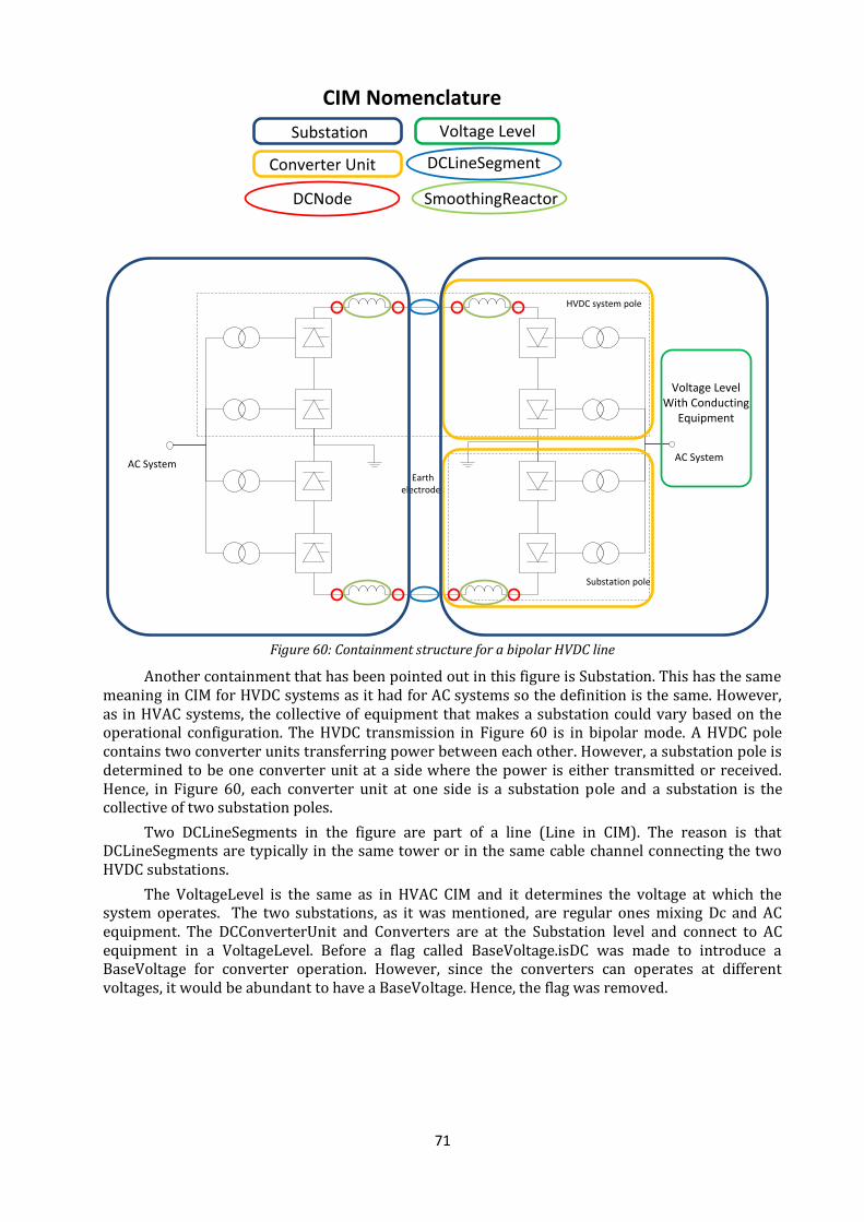
71
AC System
HVDC system pole
Substation pole
Earth electrodes
AC System
Substation
DCNode
Converter Unit
CIM Nomenclature
Voltage Level With Conducting
Equipment
Voltage Level
DCLineSegment
SmoothingReactor
Figure 60: Containment structure for a bipolar HVDC line
Another containment that has been pointed out in this figure is Substation. This has the same meaning in CIM for HVDC systems as it had for AC systems so the definition is the same. However, as in HVAC systems, the collective of equipment that makes a substation could vary based on the operational configuration. The HVDC transmission in Figure 60 is in bipolar mode. A HVDC pole contains two converter units transferring power between each other. However, a substation pole is determined to be one converter unit at a side where the power is either transmitted or received. Hence, in Figure 60, each converter unit at one side is a substation pole and a substation is the collective of two substation poles.
Two DCLineSegments in the figure are part of a line (Line in CIM). The reason is that DCLineSegments are typically in the same tower or in the same cable channel connecting the two HVDC substations.
The VoltageLevel is the same as in HVAC CIM and it determines the voltage at which the system operates. The two substations, as it was mentioned, are regular ones mixing Dc and AC equipment. The DCConverterUnit and Converters are at the Substation level and connect to AC equipment in a VoltageLevel. Before a flag called BaseVoltage.isDC was made to introduce a BaseVoltage for converter operation. However, since the converters can operates at different voltages, it would be abundant to have a BaseVoltage. Hence, the flag was removed.
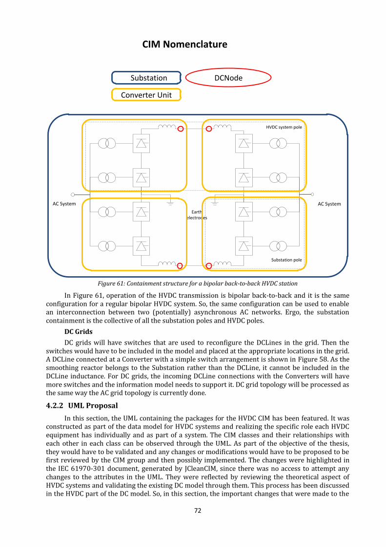
72
AC System
HVDC system pole
Substation pole
Earth electrodes
AC System
Substation DCNode
Converter Unit
CIM Nomenclature
Figure 61: Containment structure for a bipolar back-to-back HVDC station
In Figure 61, operation of the HVDC transmission is bipolar back-to-back and it is the same configuration for a regular bipolar HVDC system. So, the same configuration can be used to enable an interconnection between two (potentially) asynchronous AC networks. Ergo, the substation containment is the collective of all the substation poles and HVDC poles.
DC Grids
DC grids will have switches that are used to reconfigure the DCLines in the grid. Then the switches would have to be included in the model and placed at the appropriate locations in the grid. A DCLine connected at a Converter with a simple switch arrangement is shown in Figure 58. As the smoothing reactor belongs to the Substation rather than the DCLine, it cannot be included in the DCLine inductance. For DC grids, the incoming DCLine connections with the Converters will have more switches and the information model needs to support it. DC grid topology will be processed as the same way the AC grid topology is currently done.
4.2.2 UML Proposal
In this section, the UML containing the packages for the HVDC CIM has been featured. It was constructed as part of the data model for HVDC systems and realizing the specific role each HVDC equipment has individually and as part of a system. The CIM classes and their relationships with each other in each class can be observed through the UML. As part of the objective of the thesis, they would have to be validated and any changes or modifications would have to be proposed to be first reviewed by the CIM group and then possibly implemented. The changes were highlighted in the IEC 61970-301 document, generated by JCleanCIM, since there was no access to attempt any changes to the attributes in the UML. They were reflected by reviewing the theoretical aspect of HVDC systems and validating the existing DC model through them. This process has been discussed in the HVDC part of the DC model. So, in this section, the important changes that were made to the
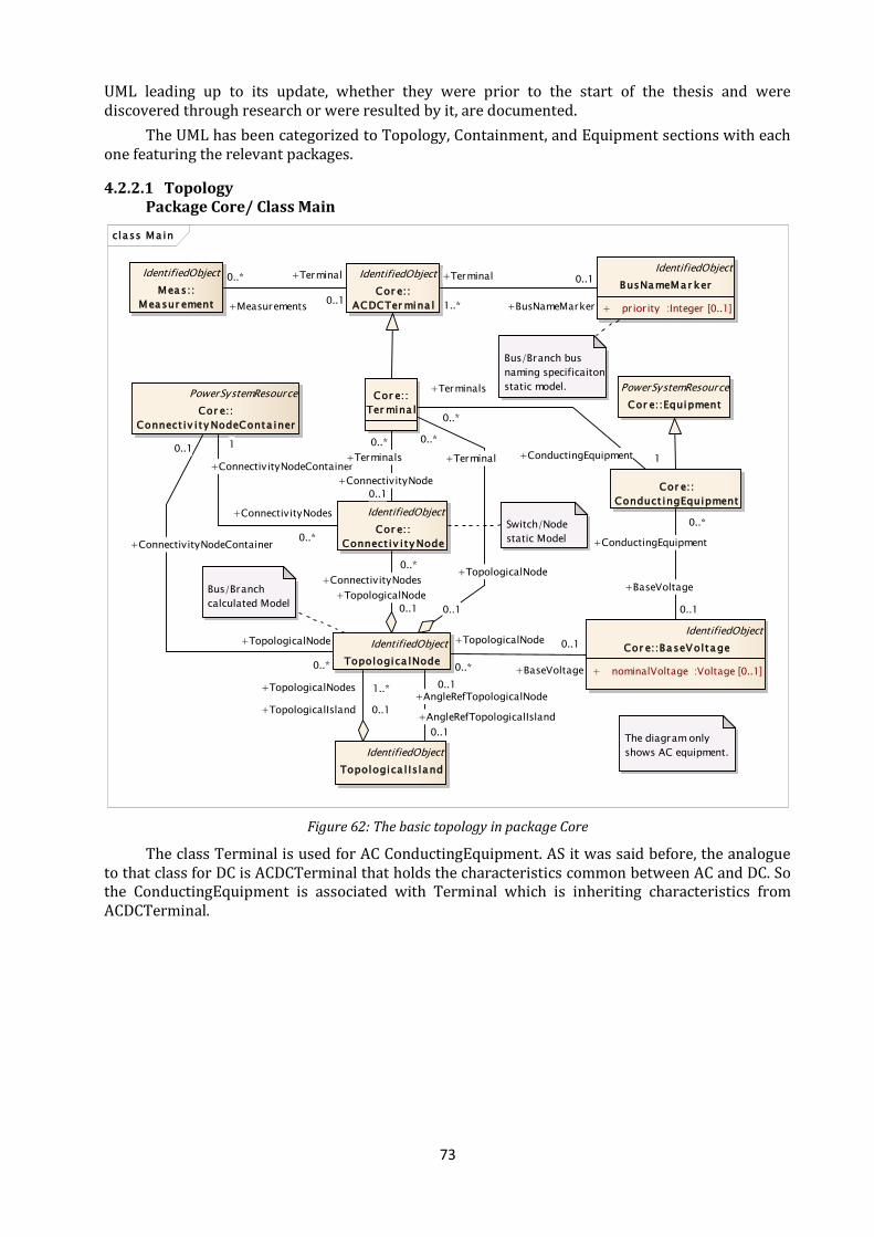
73
UML leading up to its update, whether they were prior to the start of the thesis and were discovered through research or were resulted by it, are documented.
The UML has been categorized to Topology, Containment, and Equipment sections with each one featuring the relevant packages.
4.2.2.1 Topology Package Core/ Class Main
Figure 62: The basic topology in package Core
The class Terminal is used for AC ConductingEquipment. AS it was said before, the analogue to that class for DC is ACDCTerminal that holds the characteristics common between AC and DC. So the ConductingEquipment is associated with Terminal which is inheriting characteristics from ACDCTerminal.
cla ss Ma in
Switch/Node
static Model
IdentifiedObject
Cor e::
Connect iv i ty Node
PowerSystemResource
Cor e::
Connect iv i ty NodeConta iner
Cor e::
Ter mina l
Bus/Branch
calculated Model
IdentifiedObject
Topologica lNode
IdentifiedObject
Meas::
Measur ement
Cor e::
Conduct ingEquipment
IdentifiedObject
Topologica l Island
IdentifiedObject
BusNameMar ker
+ priority :Integer [0..1]
PowerSystemResource
Cor e::Equipment
Bus/Branch bus
naming specificaiton
static model.
IdentifiedObject
Cor e::
ACDCTer mina l
IdentifiedObject
Cor e::BaseVoltage
+ nominalVoltage :Voltage [0..1]
The diagram only
shows AC equipment.
+ConnectivityNodes
0..*
+ConnectivityNodeContainer
1
+TopologicalNodes 1..*
+TopologicalIsland 0..1
+BaseVoltage
0..1
+ConductingEquipment
0..*
+Terminals
0..*
+ConductingEquipment 1
+AngleRefTopologicalIsland
0..1
+AngleRefTopologicalNode0..1
+ConnectivityNodes
0..*
+TopologicalNode
0..1
+Terminal
0..*
+TopologicalNode
0..1
+TopologicalNode
0..* +BaseVoltage
0..1+TopologicalNode
0..*
+ConnectivityNodeContainer
0..1+Terminals
0..*
+ConnectivityNode
0..1
+BusNameMarker
0..1+Terminal
1..*+Measurements
0..* +Terminal
0..1
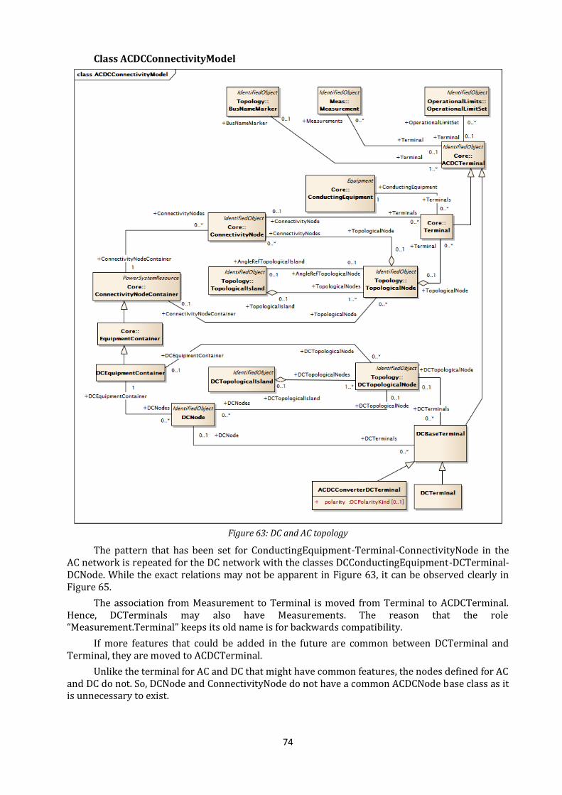
74
Class ACDCConnectivityModel
Figure 63: DC and AC topology
The pattern that has been set for ConductingEquipment-Terminal-ConnectivityNode in the AC network is repeated for the DC network with the classes DCConductingEquipment-DCTerminal-DCNode. While the exact relations may not be apparent in Figure 63, it can be observed clearly in Figure 65.
The association from Measurement to Terminal is moved from Terminal to ACDCTerminal. Hence, DCTerminals may also have Measurements. The reason that the role “Measurement.Terminal” keeps its old name is for backwards compatibility.
If more features that could be added in the future are common between DCTerminal and Terminal, they are moved to ACDCTerminal.
Unlike the terminal for AC and DC that might have common features, the nodes defined for AC and DC do not. So, DCNode and ConnectivityNode do not have a common ACDCNode base class as it is unnecessary to exist.

75
4.2.2.2 Containment Class DCContainment
Figure 64: HVDC Containment
DCConductingEquipment has the same features as Equipment in AC so it can be put in a Substation, VoltageLevel, or Bay. However, the DC topology requires DCNodes which exist only in a DCEquipmentContainer. Hence DCConductingEquipment resides in DCConverterUnits or DCLines that are subclasses to DCEquipmentContainer. So, in this case it inherits the DCNodes needed for DC topology through the inheritance between DCConverterUnit, DCEquipmentContainer in package DC, and EquipmentContainer in package Core.
DCLines can span between Substations since unlike DCConverterUnits, they are not part of the Substation. Moreover, DCConverterUnits can be associated with AC equipment in a Substaion. Therefore, both AC and DC equipment can coexist in Substations.
The back-to-back configuration in Figure 61 is handled by placing the DCLineSegment in the Subsation instead of a DCLine.
The CIM containment model is open and the guidelines for which class shall contain what equipment are as follows:
DCLineSegments are allowed in Substaions (back to back configuration) and DCLines.
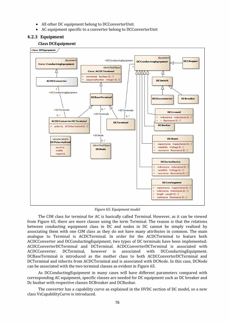
76
All other DC equipment belong to DCConverterUnit. AC equipment specific to a converter belong to DCConverterUnit
4.2.3 Equipment
Class DCEquipment
Figure 65: Equipment model
The CIM class for terminal for AC is basically called Terminal. However, as it can be viewed from Figure 65, there are more classes using the term Terminal. The reason is that the relations between conducting equipment class in DC and nodes in DC cannot be simply realized by associating them with one CIM class as they do not have many attributes in common. The main analogue to Terminal is ACDCTerminal. In order for the ACDCTerminal to feature both ACDCConverter and DCConductingEquipment, two types of DC terminals have been implemented: ACDCConverterDCTerminal and DCTerminal. ACDCConverterDCTerminal is associated with ACDCConverter. DCTerminal, however is associated with DCConductingEquipment. DCBaseTerminal is introduced as the mother class to both ACDCConverterDCTerminal and DCTerminal and inherits from ACDCTerminal and is associated with DCNode. In this case, DCNode can be associated with the two terminal classes as evident in Figure 65.
As DCConductingEquipment in many cases will have different parameters compared with corresponding AC equipment, specific classes are needed for DC equipment such as DC breaker and Dc busbar with respective classes DCBreaker and DCBusbar.
The converter has a capability curve as explained in the HVDC section of DC model, so a new class VsCapabilityCurve is introduced.
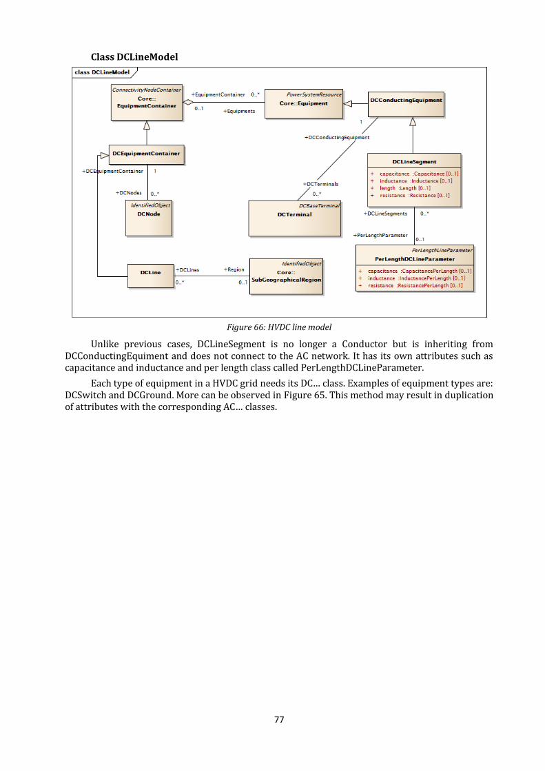
77
Class DCLineModel
Figure 66: HVDC line model
Unlike previous cases, DCLineSegment is no longer a Conductor but is inheriting from DCConductingEquiment and does not connect to the AC network. It has its own attributes such as capacitance and inductance and per length class called PerLengthDCLineParameter.
Each type of equipment in a HVDC grid needs its DC… class. Examples of equipment types are: DCSwitch and DCGround. More can be observed in Figure 65. This method may result in duplication of attributes with the corresponding AC… classes.
78
5 jCleanCim
jCleanCim is an open source tool for validation and documentation generation from Enterprise Architect CIM and IEC61850 UML models. It was developed by Tatjana Kostic from ABB Switzerland. [26]
jCleanCim was initially developed to perform validation of CIM EA model file, then extended to do clean-up of left-overs from Rose and to show some basic statistics (thus addressing combined CIM issue #1103). Finally, it has been extended to allow for IEC (and custom) document generation, mainly driven by special needs of generating IEC 61850-7-3 and IEC 61850-7-4 from UML model developed by ABB and handed over to IEC TC57 WG19 in October 2009.
Since 01v05, jCleanCim has received functionalities to generate documentation for different CIM UML model. It has been used by CIM editors of IEC TC57 WG13, WG14 and recently WG16 to generate IEC 61970-301, IEC 61968-11 and IEC 62325-301 documents, respectively, as well as for the documentation describing CIM extensions developed in the European FP7 project.
Since September 2010, it has also been used by 61850 UML taskforce of WG10 to validate IEC 61850 UML and to automatically generate IEC 61850-7-4 and IEC 61850-7-3. As other IEC working groups start moving their IEC 61850-based specifications to UML as master model, jCleanCim will allow for automatic document generation for these, as well. Furthermore, since 01v06, the tool supports serialisation of the UML model of IEC 61850 to an XML format, that would be suitable for publishing on the web, and in support of the WebAccess taskforce of WG10. As a by-product, the same feature is available for CIM UML model.
jCleanCim has four main functions:
1. validation of a UML model provided in an .eap file, bulk or per IEC TC57 WG, 2. calculation and printing of statistics of the UML model, 3. generation of MS Word documentation from the UML model, 4. generation of XML documentation from the UML model.
Intended users are primarily those who edit CIM UML and publish its documentation, thus:
• official IEC CIM model editors, responsible for maintaining the CIM information model (UML) and for generating official IEC documents, and,
• those who define custom non-standard CIM extensions who want to ensure they have followed standard CIM rules and who want to generate documentation for those extensions.
In the jCleanCim software package there are 3 separate distributions:
1. bin distribution. It is aimed mainly for jCleanCim users and doesn’t require any additional software or programming skills.
2. eclipse distribution. It’s aimed for jCleanCim developer and users, who has experience of working with Eclipse IDE. It requires installation of “Eclipse IDE for Java Developers” software. On the other hand, this distribution provides the most comfortable way of working with jCleanCim application with console output and interface.
3. src distribution. It’s aimed for JCleanCim developers and users familiar with Apache Ant software, that has XML-based build structure.
5.1 jCleanCim configuration
To configure any run of jCleanCim application, you use the standard Java properties file available in the Config directory. Default name for that properties file is config.properties and you can override this default with a command line argument if you want to use different stable configurations for different jCleanCim runs.
Available Java properties allow you to configure how to run jCleanCim: which main functions to run or not (validation, statistics, document generation), and to fine tune their execution. At present, this is the most comfortable way to configure a run of jCleanCim.
Because this is a java application, every property found in the #DEFAULT_PROPS_FILE_NAME file can be overwritten when launching the application by providing one or more -

79
D<propertyName>=<propertyValue> statements immediately after the Java command, but if there are many properties to configure, it is simpler to do it in the #DEFAULT_PROPS_FILE_NAME file.
The values obtained from properties have been validated and stored in appropriate format in the constructor. For instance, "true" is read as string and stored as boolean; comma-separated string read from file is stored as a list of strings; absolute file paths are produced from the simple file names. These are then made available through methods to the application.
The original default properties file config.properties contains reasonable defaults, and several tested configurations are commented. By default, jCleanCim will run validation and statistics on default model file (located in the input directory), and will not generate any documentation.
5.1.1 Logging configuration
Config directory contains also the logging configuration file log4j.xml. The console output level is set up to INFO (within the element appender name="CONSOLE"... ), and the level for everything else to the most verbose, TRACE (within the element logger name="org.iec.tc57.jcleancim" ). The first time jCleanCim application is run, the Log directory gets created automatically.
5.1.2 UML model validation and statistics
In order to run the specific function of jCleanCim, the appropriate main property in the config/config.properties file needs to be set, i.e.:
validation.on,
statistics.on
docgen.on .
In order to proceed with jCleanCim application, you have to provide a valid EA model file name in the property model.filename. The EA model file is expected to be on the jCleanCim classpath, so the best is to put the file in the input directory which is already set to be on the classpath.
Typical usage will be to first enable validation and statistics mode after you have edited the model, then address the problems in the model, and revalidate before releasing. Here is an example of a minimum config.properties file to do that:
model.filename = base-small.eap
validation.on = true
statistics.on = true
If you have a big model, with potentially parts that are informative, you may want to set a filter and perform initial validation of your changes for only some top-level packages. For instance, to validate only standard CIM packages IEC61970 and IEC61968, you would set the validation.scope property so:
validation.scope = WG13, WG14
and to validate only custom (non-IEC) extensions:
validation.scope = OTHER_CIM, OTHER_IEC61850
It is recommended to validate the full content of the EA model (by leaving the value of validation.scope property empty) at least before releasing the model, to ensure there are no cross-package issues.
5.1.3 Input and Output Files
Input files are mainly expected to be available in any place that is on the classpath. By convention, the directory input is configured under the project root to be on the classpath; this eliminates the need for absolute paths. The application never modifies anything under input directory. Files searched on the classpath are:
model file #KEY_MODEL_FILENAME,

80
XML schema for document generation (defined as default: #DEFAULT_WEBACCESS_SCHEMA_FILENAME), or
MS Word template file: #KEY_DOCGEN_WORD_IN_TEMPLATE.
Output files are created in a separate directory, #OUTPUT_DIR_NAME, under the current execution path obtained with the Java system property org.iec.tc57.jcleancim.util.Util #USER_DIR_KEY. If such a directory is not available, like in case of a fresh installation, it gets automatically created. The constructor of this class completes all the tricks related to files, both input and output, and once it completed successfully, it is sure that all the file absolute paths are valid. Furthermore, if an output file (to be produced by the current run of jCleanCim) already exists in the #OUTPUT_DIR_NAME directory, it will be renamed already in the constructor to ensure that it does not get overwritten later on.
5.1.4 MS Word documentation generation
To generate IEC (or custom) MS Word documentation from the UML model, in addition to the model file name in config/config.properties the names for template (input) file, the resulting (output) file have to be defined and document generation should be enebaled by setting the property docgen.on = true .
The template file is a regular MS Word document (not Word template with .dot extension), in which there are Placeholders to control what jCleanCim should pick from the UML model and print into MS Word document.
Placeholders
Templates for doc generation have to use labels to indicate where to insert the documentation of what element of the UML model into the output document. Currently needed and recognized labels to be used in the input templates are in the following format:
startUmlDiagram.{packageName}.{diagramName}.endUml
startUmlAttribute.{className}.{attributeName}.endUml
startUmlFile.endUml
startUmlPackage.{packageName}.endUml
The tokens enclosed in curly braces are the names of UML elements designating what needs to be inserted in place of the whole above string.
This format avoids the necessity to define bookmarks in the input document (tedious and error-prone) and makes it simple to sequentially search the input document and insert the text and diagrams as they come.
jCleanCim conducts the following procedure in generating the document:
• copy the template file into the projects output directory, created automatically the document generation,
• rename the copied file to the name given in the properties file, • fill up the copy with the contents from the EA model in place of the placeholders.
jCleanCim allows safely to run document generation several times with the same name of the output file, without overwriting existing output files. If the output file exists with the same name, jCleanCim will rename it by appending a system nanosecond time. It can be a little inconvenient, those discarded files needs to be deleted from the output directory from time to time, but on the other hand the history of generation can be easily tracked.
It can be useful to disable validation and statistics when enabling document generation to reduce the size of log file and to make it console, focused on document generation only.
Since document generation takes pretty long, it is reasonable to use docgen.analysePlaceholders property to ensure that the placeholders in the template are correct, without generating the full package content. The minimum configuration to do this for a CIM model is given below:
model.filename = base-small.eap

81
docgen.on = true
profiles.docgen.on =
docgen.inTemplate = base-small-template.doc
docgen.outDocument = base-small.doc
docgen.analysePlaceholders = true
Running only placeholder analysis ( docgen.analysePlaceholders=true ) will still produce the output document, but without UML package contents (classes, attributes, etc.). More importantly, that half-baked output document will contain placeholder errors, if any - do text search for string "$ERROR".
After you have fixed the placeholders in the template, you can reset docgen.analysePlaceholders to empty string to generate the full documentation. When generating official IEC documentation, the template should contain the IEC styles. To prevent MS Word exceptions when generating non-IEC documentation for extensions, jCleanCim defines default MS Word styles as replacement for the IEC styles. So, for example, 'Caption' is used if 'FIGURE-title' and 'TABLE-title' are not present in the template, or 'Normal' is used if 'PARAGRAPH' is not present. Below is the code snippet of the static initialiser for Style for the full list of default mappings: first argument is IEC style name and the second is the MS Word default style:
para("PARAGRAPH", "Normal"),
fig("Picture", "Normal"),
figcapt("FIGURE-title", "Caption"),
tabcapt("TABLE-title", "Caption"),
tabhead("TABLE-col-heading", "Normal"),
tabcell("TABLE-cell", "Normal"),
h1("Heading 1", "Heading 1"),
h2("Heading 2", "Heading 2"),
h3("Heading 3", "Heading 3"),
h4("Heading 4", "Heading 4"),
h5("Heading 5", "Heading 5"),
h6("Heading 6", "Heading 6"),
h7("Heading 7", "Heading 7"),
h8("Heading 8", "Heading 8"),
h9("Heading 9", "Heading 9");
It is essential to use correct styles for paragraphs containing figure and table captions in the template, because jCleanCim must deduce the number of figures and tables already existing in the template to calculate on the fly the correct numbering for new figures and tables (when inserting/appending the documentation for the UML model elements and diagrams). If jCleanCim throws an exception during document generation, it is very likely that the MS Word threw exception due to inexisting/negative number for the figure or table caption.
Since version 01v03, jCleanCim has the MS Word application run in background by default (which is faster than having the window visible and updating all the time). It is important to mention that the jCleanCim is compatible only with English-based MS Word application.
5.2 The jCleanCim configuration for document generation for IEC 61970-301
The Java properties file that is required to run jClean Cim to generate documentation of IEC 61970-301 standard can be divided in the following properties groups:
Model-related properties
These properties specify the UML or other model to work with:

82
• Property #KEY_MODEL_FILENAME holds the name of the EA file containing UML model. This file is expected to be found on the classpath (in the INPUT directory). The value is ignored if the application is invoked with the -m<myModel.eap> command line argument. The value specified with this property is useful if you always use the same configuration file, so you need not type command line argument. A valid UML class diagram is required for every scenario.
model.filename = iec61970cim16v29_iec61968cim12v08_iec62325cim03v01a.eap
• Property #KEY_MODEL_BUILDER allows you to choose the most performant loading of the model .eap file given your usage requirements. For full support of diagram and XMI export use ModelBuilderKind.sqlxml. This implementation is based on SQL queries for reading the model .eap file. It is almost order of magnitude faster than the regular API calls (option ModelBuilderKind.japi). The fastest implementation is ModelBuilderKind.db without export diagrams or XMI. Since the diagram export from UML model is required for IEC 61970-301 documentation, the first option has to be chosen:
model.builder = sqlxml
Top-level properties
These properties select the functionality to execute. The control of execution gets by enabling ("true") or disabling ("false" = value, "" = value omitted, null = whole property absent) one or more of the top level options.
• Property #KEY_XMIEXPORT_ON allows to export the .eap model to the three XMI formats (XMI 1.1, XMI 2.1 and CIMTool, XMI 1.4/Rose);
• Property #KEY_VALIDATION_ON allows to run model validation; this option is independent from other top-level options.
• Property #KEY_STATISTICS_ON allows to run model statistics; this option is independent from other top-level options.
• Property #KEY_DOCGEN_ON allows to run document generation from UML model (as required for IEC61968-11, IEC61970-301 or IEC61850-7-4).
• If #KEY_DOCGEN_ON = "true" and #KEY_PROFILES_DOCGEN_ON = "true", the jCleanCim runs MS Word document generation from one or more CIM RDF/OWL profiles.
The following parameters of top-level properties are required:
xmiexport.on =
validation.on = true
statistics.on = true
docgen.on = true
profiles.docgen.on =
Statistics properties
These options control the displaying of statistics and are applicable only if value in property #KEY_STATISTICS_ON = "true". There are only two boolean options, both applicable to CIM only. In CIM, almost every class inherits from IEC61970::Core::IdentifiedObject, and most of attributes have as a type some class from IEC61970::Domain package. These two options allow, when set to "true", to skip displaying these obvious cross-WG dependencies and avoid unnecessary noise in the output:
statistics.cim.ignoreIdObjectInheritance = true
statistics.cim.ignoreDomainClassAttributes = true
MS Word document generation properties
These options specify and control the generation of MS Word document when property #KEY_DOCGEN_ON is set to "true". Depending on the value in #KEY_PROFILES_DOCGEN_ON, the document will be generated from the UML model as default (if #KEY_PROFILES_DOCGEN_ON = "false", "", null), or from multiple profiles (if #KEY_PROFILES_DOCGEN_ON = "true").
Here are MS Word document generation properties:

83
Property #KEY_DOCGEN_INCLUDE_INFORMATIVE, if set "true", allows to include informative elements from UML model into generated document. By default ("false", "", null), these are skipped for document generation.
• Property #KEY_DOCGEN_INCLUDE_NON_PUBLIC, if set "true", allows to include private, package-private or protected UML elements into generated document. By default ("false", "", null), these are skipped for document generation.
Property #KEY_DOCGEN_WORD_USE_DOC_FORMAT, when enabled, forces usage of the slow COM API for MS Word, in case if the fast OpenXML (.docx) format is not available.
• Property #KEY_DOCGEN_WORD_SAVE_REOPEN_EVERY gives the number of tables (and implicitly, table captions) to write before saving, closing and reopening the auto-generated document. This option was implemented to improve the performance of MS Word document generation for extremely large documents (more than ~200 tables). Document generation procedure slows down exponentially with the number of captions inserted. Default value is -1, which means no close/reopen will happen. It’s suggested to set this value between 12 and 27.
• Property #KEY_DOCGEN_WORD_ANALYSE_PLACEHOLDERS, if set "true", allows you to only analyse ("validate") your input template and get hint on errors. This is useful when e.g. updating template with placeholders for new diagrams: if you have a typing error and specify the value in the placeholder which does not exist in the UML model, an output MS Word document will be generated by replacing the placeholders not with real content from UML, but with the actual names from UML that would be used; or with ERROR description in case the placeholder value is invalid. This is very handy to run before actually generating the full documentation if the template is updated. The output document containing no "ERROR" indicates that all the placeholders are OK.
• Property #KEY_DOCGEN_WORD_PRINT_HTML, if set "true", will allow to respect mark-up formatting in the documentation of elements in the UML repository when generating MS Word document.
The parameters of MS Word document generation properties for IEC 61970-301 standard documentation are:
docgen.includeInformative =
docgen.includeNonPublic =
docgen.word.printHtml =
docgen.word.analysePlaceholders = true
docgen.word.useDocFormat =
docgen.word.inTemplate = template_iec61970-301v29.docx
docgen.word.outDocument = iec61970-301_iec61970cim16v29-tool01v09.docx
docgen.word.saveReopenEvery = 27

84
6 Practical Realization of CIM Use
The next step after generating the standard document is to implement the model to a network management application. The application in ABB Ventyx is the Network Manager system includes many SCADA based applications for planning and operation. Use of network manager can be applied to exchanging data between Transmission System Operators (TSO) and it is an advanced technology one that incorporates standardized representation of existing electric models both AC and DC. Other than network manager, companies and institutes use other means and other standards to exchange data models between each other and one way is to use instance diagrams based on data models. An example of this method is what is being applied by ENTSO-E and will be discussed in this chapter. It should be mentioned that implementing the DC model into the network manager at ABB was one of the tasks regarding the thesis, however due to the fact that it is a proprietary software, it cannot be published public and thus its related chapter has been removed.
6.1 Common Information Model for Grid Models Exchange
“ENTSO-E is the European Network of Transmission System Operators, represents 41 electricity transmission system operators from 34 countries across Europe. ENTSO-E promotes closer cooperation across Europe’s TSOs to support the implementation of EU energy policy and achieve Europe’s energy and climate policy objectives, which are changing the very nature of the power system.”[31]
As it was mentioned before, data exchange is essential to maintaining a stable network. In the case of ENTSO-E, studies would have to be run on the European grid for analysis of the current state and processes related to the future and that is based on data exchange between TSOs. The CIM for grid exchange can be done for fulfilling that purpose. “Common Grid Model Exchange Standard (CGMES) is an ENTSO-E standard used for the exchange of power system models between TSOs for study purposes in Europe.”[30]
Exchange of grid models is a complex process which includes the following information to be exchanged:
Equipment information, containing power system equipment data Topology information, containing topology related information for the grid elements Information on power system state variables, which is the results from initial load flow
simulations of the system Steady state hypothesis information, valid for newer standards that contains information on
load and generation values as well as other input parameters necessary to perform load flow simulations.
Moreover, the information related to the dynamics, diagram layout and geographical location for elements in the power system can also be included in the data for grid model exchange. ENTSO-E standards such as CGMES have the role of defining the interface between ENTSO-E members’ software in order to exchange power system modelling information as required by the ENTSO-E and TSO business processes. CGMES along with other ENTSO-E standards for grid models exchange are based on the current or future developed IEC CIM standards:
IEC 61970-552: CIM XML Model Exchange Format IEC 61970-301: Common Information Model (CIM) Base IEC 61970-302: Common Information Model for Dynamics Specification IEC 61970-452: CIM Static Transmission Network Model Profiles IEC 61970-453: Diagram Layout Profile IEC 61970-456: Solved Power System State Profiles IEC 61970-457: CIM for Dynamics Profile IEC 61968-4: Application integration at electric utilities – System interfaces for
distribution management
“The Common Grid Model Exchange Standard (CGMES) is a superset of the IEC Common Information Model (CIM) standard. It was developed to meet necessary requirements for TSO data

85
exchanges in the areas of system development and system operation and was initially published in December 2013.”[32] It is to be used as a baseline exchange standard for the implementation of the Common Grid Model (CGM) methodologies. CGMES will be mainly applied by applications that deal with power system data management as well as applications regarding the following studies:
Load flow and contingency analyses Short circuit calculations Market information and transparency Capacity calculation for capacity allocation and congestion management Dynamic security assessment
The CGMES Conformity Assessment Framework was developed and approved by ENTSO-E as the conformity of applications used for operational and system development exchanges with the CGMES is crucial in order for each application to achieve interoperability. The framework is essentially a principle guideline for assessing application’ CGMES conformity. A Conformity Assessment Process is further used by ENTSO-E to ensure of proper implementation of CGMES by suppliers of the applications used by TSOs.
6.2 Exchange Process
Data models exchange is necessary to happen in different levels. A pan-European model exchange level covers the territory of all TSOs. Regional model exchange can occur between different TSOs in one of more synchronous areas. On the national level, the model exchange includes interfaces between TSOs and DSO (Distribution System Operator)s as well as between different DSOs.
As it was mentioned before the purpose of the model exchange, in addition to exchange the data between different authorities with efficiency, is to perform common studies using shared data. This means that the parties involved in the process should be able to perform the same types of studies and also be able to share project tasks between different parties regardless of the kind of power system application they are using for analysis. Therefore, achieving interoperability between different applications used in the exchange process is crucial to fulfil the goal of seamless data exchange and acquiring comparable study results when using the data.
The CGMES covers these ENTSO-E and TSO business processes by defining the main types of exchange valid for a particular study or process:
Exchange of Boundary set: “A boundary set contains all boundary points (connectivity nodes placed on a tie line or in a substation) necessary for a given grid model exchange”.[30] In order to prepare an exchange of an internal TSO model and to assemble a common grid model, it is necessary to exchange a Boundary Set.
Exchange of an Internal TSO model: Each TSO would have to provide models of its internal territory as a requirement for a number of business processes. For that purpose, a TSO is treated as a single model authority set and would then be able to exchange all profiles defined in the CGMES. The internal model would have to be prepared in a way to be combined easily with other TSO internal models to create a complete model used for analysis later.
Exchange of a Common Grid Model: A common grid model refers to the concept of having one model which can be used for multiple purposes. The standard describes the process of creating an assembly of multiple TSOs Individual Common Grid Model (ICGM) of their responsible territory into a regional or pan-European model. Different business processes need specific implementation of the profiles part of the CGMES and the exchange of respective instance files to meet interoperability inside the business process. The Common Grid Model meta-model description ensures interoperability across the business process.
The ENTSO-E and TSO business processes include for example, system development planning, protection planning, operational planning, operation, fault study/simulation, market operation, etc.
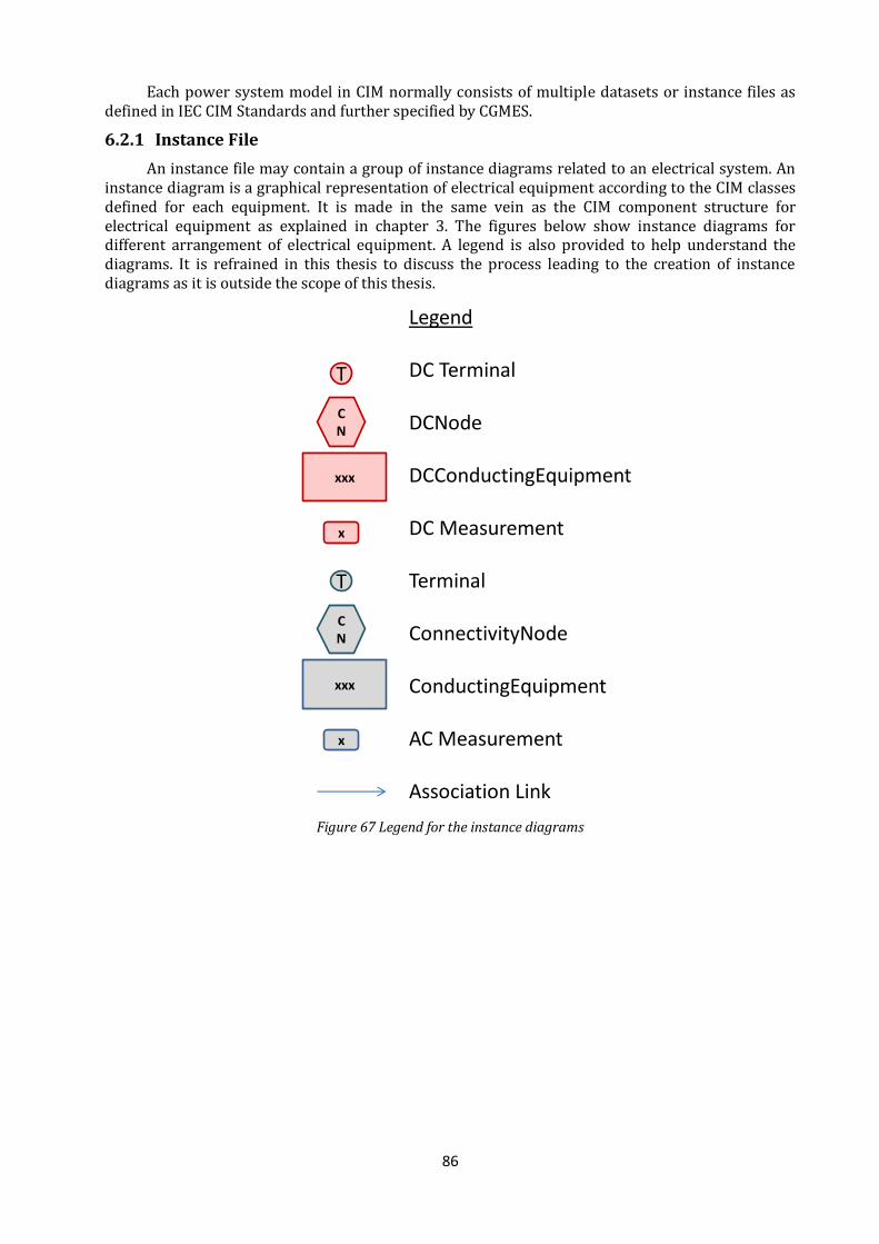
86
Each power system model in CIM normally consists of multiple datasets or instance files as defined in IEC CIM Standards and further specified by CGMES.
6.2.1 Instance File
An instance file may contain a group of instance diagrams related to an electrical system. An instance diagram is a graphical representation of electrical equipment according to the CIM classes defined for each equipment. It is made in the same vein as the CIM component structure for electrical equipment as explained in chapter 3. The figures below show instance diagrams for different arrangement of electrical equipment. A legend is also provided to help understand the diagrams. It is refrained in this thesis to discuss the process leading to the creation of instance diagrams as it is outside the scope of this thesis.
CN
T
xxx
xxx
CN
T
Legend
DC Terminal
DCNode
DCConductingEquipment
DC Measurement
Terminal
ConnectivityNode
ConductingEquipment
AC Measurement
Association Link
x
x
Figure 67 Legend for the instance diagrams
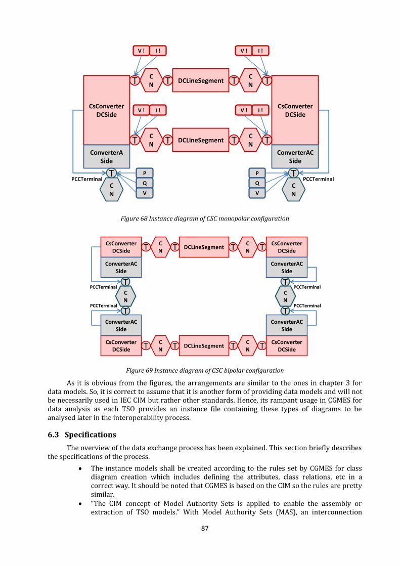
87
CsConverterDCSide
ConverterACSide
T
CN
CN
DCLineSegment T
T
TCNT
CsConverterDCSide
ConverterASide
PCCTerminalCN
TPCCTerminal
P
Q
V
P
Q
V
V ! I ! V ! I !
TCN
DCLineSegment TTCNT
V ! I ! V ! I !
Figure 68 Instance diagram of CSC monopolar configuration
CsConverterDCSide
ConverterACSide
T
CN
CN
DCLineSegment T
T
TCNT
CsConverterDCSide
ConverterACSide
CN
T
CsConverterDCSide
ConverterACSide
TCN
DCLineSegment T
T
TCNT
CsConverterDCSide
ConverterACSide
T
PCCTerminal
PCCTerminal
PCCTerminal
PCCTerminal
Figure 69 Instance diagram of CSC bipolar configuration
As it is obvious from the figures, the arrangements are similar to the ones in chapter 3 for data models. So, it is correct to assume that it is another form of providing data models and will not be necessarily used in IEC CIM but rather other standards. Hence, its rampant usage in CGMES for data analysis as each TSO provides an instance file containing these types of diagrams to be analysed later in the interoperability process.
6.3 Specifications
The overview of the data exchange process has been explained. This section briefly describes the specifications of the process.
The instance models shall be created according to the rules set by CGMES for class diagram creation which includes defining the attributes, class relations, etc in a correct way. It should be noted that CGMES is based on the CIM so the rules are pretty similar.
“The CIM concept of Model Authority Sets is applied to enable the assembly or extraction of TSO models.” With Model Authority Sets (MAS), an interconnection

88
model can be divided to separate sets of objects allowing for different parties to take responsibility for different parts of a common grid model. Each object instance is assigned to one and only one MAS.
Each type of instance file shall have a file header. The IEC 61970-552 specification is used to format a file which contains only the
objects from one MAS. Nine different profiles in CGMES are created based on the instance files in order to
ensure the correct exchange of the data models. The CGMES profiles are based on the CIM profiles and contain the similar set of rules which in turn are applied to the instance files.
Extensions to the profiles are made in order to accommodate the complexity and specificity of the ENTSO-E business processes. The extensions are defined in the frame of the CGMES which is based on IEC CIM.
Files should follow the rules set by CGMES on how to be constructed and ready for exchange.
Model containing the boundary sets will be exchanged following the guidelines set by CGMES.
A model will be assembled which will be the common grid model (solved or unsolved power system model) and contains information from more than one model authority set. Dividing the files per MAS creates better flexibility when it comes to how complete the assembled models are for formed.
Power flow simulations and other analyses can be done on the model RDF/XML validity is used to determine the model’s verification. Naming convention which is an important part of any profile and renders it
understandable and suitable for data exchange is undergone for the model according to CGMES regulations.
6.4 Governance of CGMES
Governing process of CGMES can be divided into different sub processes which can be seen in the figure and will be explained in the following.
Figure 70 CGMES process diagram
89
6.4.1 Standardisation an interoperability process
The CGMES covers many cases and is in use for many business processes. The standard would have to comply to the international standards so the development process interacts with IEC to ensure most of the functionalities of the CGMES are accepted and released in the IEC CIM standards. Nevertheless, ENTSO-E and TSOs have some specific requirements which would not be part of the IEC CIM standards and they are satisfied by ENTSO-E CIM extensions which are part of the CGMES profiles. The changes that happen to the model exchange requirements over time as a result of the development of business processes would bring changes to the CGMES and its profiles. In order to structure the process to standardise the profiles and CGMES, the changes shall be implemented either as ENTSO-E extensions or realised during CGMES interoperability tests.
6.4.2 Approval process
The ENTSO-E board approves major and minor versions of the CGMES and its profiles. The approval triggers the conformity assessment process of the version of CGMES. The ENTSO-E bodies; System Development Committee (SDC) and System Operations Committee (SOC) recommend changes of the CGMES to the board and advise on which data exchange process uses which version of the CGMES. The approval process confirms that the development of the CGMES has reached a milestone and could be used for planning exchanges or can set a deadline for a certain business process (which could be data exchange) to be switched from one version of the CGMES to another. This approval follows the successfully completed conformity assessment processes on a certain version of the CGMES.
6.4.3 Conformity assessment
In order for tools to be labeled compliant with a given profile part of the CGMES and subsequently can be used for model exchange, they would have to go through the conformity assessment process. Conformity assessment is business driven and ensures reliability of the model exchanges by confirming interoperability between applications. It is defined in the ENTSO-E CGMES Conformity Assessment Framework. Conformity assessment of each tool relies on a machine readable way of defining the validation rules and describing the constraints valid for a certain profile. Object Constraint Language (OCL) is used for this purpose.
6.4.4 Implementation process
As soon as the conformity assessment process is finalised, the version of the CGMES is implemented to be used in a business process. It is triggered by the body responsible for the model exchange. The implementation process includes a period during which TSOs shall upgrade their tools and tools and a period during which a business process gets tested with the new version of the CGMES. This is valid for operational exchanges where the exchange shall be reliable and completed more frequently than a planning model exchange process. The various profiles contained in the CGMES shall also be implemented according to a schedule depending on the business needs. Business processes shall aim to use a limited number of different versions of the CGMES in order to decrease maintenance efforts by TSOs and facilitate interoperability of data exchanges between those business processes.
6.5 Example
Showing a complete example of files that were exchanged is outside of the scope of this chapter so a section of a power system used for CGMES data exchange is presented along with an excerpt of the XML document related to that section.
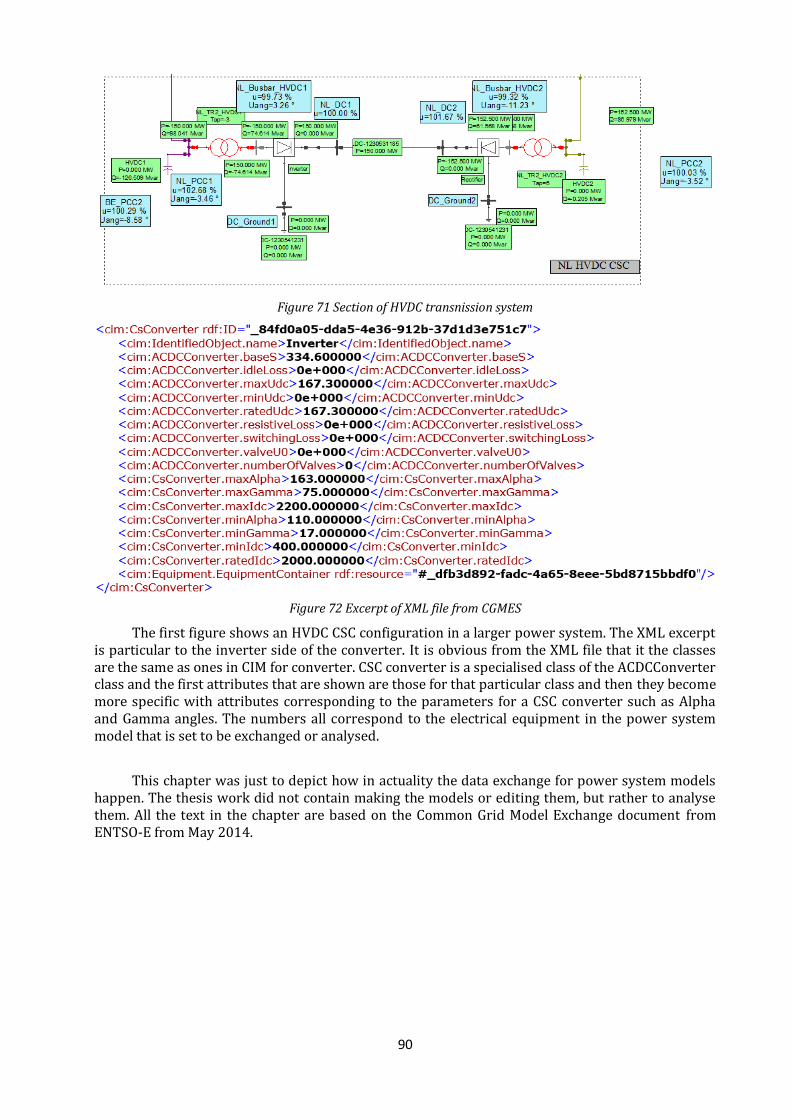
90
Figure 71 Section of HVDC transnission system
Figure 72 Excerpt of XML file from CGMES
The first figure shows an HVDC CSC configuration in a larger power system. The XML excerpt is particular to the inverter side of the converter. It is obvious from the XML file that it the classes are the same as ones in CIM for converter. CSC converter is a specialised class of the ACDCConverter class and the first attributes that are shown are those for that particular class and then they become more specific with attributes corresponding to the parameters for a CSC converter such as Alpha and Gamma angles. The numbers all correspond to the electrical equipment in the power system model that is set to be exchanged or analysed.
This chapter was just to depict how in actuality the data exchange for power system models happen. The thesis work did not contain making the models or editing them, but rather to analyse them. All the text in the chapter are based on the Common Grid Model Exchange document from ENTSO-E from May 2014.
91
7 Conclusions
In this section the summary of every chapter will be presented. The summary will be accompanied with the challenges, that were faced during the project, as well as results achieved by each chapter.
The first chapter is providing the theoretical background of HVDC technologies together with comparison of two main converter topologies: Current and Voltage source converters. The general structure and specific characteristics of both types of HVDC converters are described. The lists of main components of LCC CSC and VSC Substation Terminals along with their brief description and functionalities are elaborated. VSC converter topologies and opportunities of applying them in modern HVDC Grids are presented. The most common operating configurations of HVDC transmission system are described along with advantages and drawbacks of their application. The general overview of control methods and modes applied in HVDC converters is elaborated for both technologies. The control modes of VSC converter are analysed through the opportunities of active and reactive power flow control.
The presented academic literature and IEC documents overview yields a solid ground for further validation of preliminary developed HVDC power flow model description.
The second chapter provides the historical overview of CIM development along with important components and essential technologies applied in the CIM model. The list of IEC Committees and Working Groups responsible for maintaining different parts of CIM is accompanied with their short descriptions. The main Use cases along with development process of CIM Data Model is briefly described. The main part of the chapter elaborates the technologies used in CIM. The Unified Modelling Language (UML) is presented as an introduction of UML Infrastructure and Superstructure along with Class and Package diagrams. XML is shown as predominant language used in structuring data exchange in CIM. Basic elements and character data of XML are described. RDF Basic are very briefly mentioned.
The presented CIM structure and technology overview provides valuable means for validation of CIM Data Model in UML diagrams for HVDC Transmission systems.
The third chapter elaborates the main part of the project – HVDC power flow model description as well as CIM Data Model for HVDC systems. The first section of this chapter introduces the simplified HVDC power flow model valid for all HVDC transmission systems. The list of parameter and variables representing this power flow model is provided in the table with short description and defined type. The CSC power flow model along with specific characteristics and relations are presented. As well as for the common HVDC model the essential parameters and variables are listed in the table. The description of VSC power flow model is presented with the same structure including specific relations along with a list of essential parameters and variables.
The main challenges faced in the project are described in this chapter. One of them is connected with VSC component structure. VSC model requires providing flexibility in defining the VSC phase reactor that could include valve reactor in case of multi-level converter topology. The other challenge was to represent control modes of converter units without violating proprietary information of HVDC equipment companies.
The second section of third chapter describes the CIM Data model for HVDC Systems. The CIM Component Structure of one-line diagram of HVDC Substation terminal is presented. The essential CIM containments and their relations are described along with the correspondence to relative UML Classes. The main UML classes and packages of validated CIM DC load model is accompanied with the description of essential interconnections and class relations.
In the fourth chapter the description of jCleanCim tool is provided. The methodology of document generation based on the template for IEC 61970-301 and validated UML diagram of CIM DC load model is elaborated. The details about template extension with appropriate placeholder are mentioned. The challenge of using this tool was connected with small group of potential users and absence of proper methodology description.
92
In the fifth chapter, an example of practical data model exchange is shown based on ENTSO-E standardisation. After the introduction of the standard (CGMES), the chapter proceeds to describe the process TSOs take to create instance files of their measurement and topology data according to the rules of the standard and prepare them for exchange. The standard itself is based on IEC Common Information Model so the rules are quite similar. Further procedures including the interoperability tests and approval process and implementation are explained briefly. Examples of the instance model along with a part of a single line diagram from a power transmission system are shown.
The final output of the project is the generated documentation for IEC 61970 Energy Management System Application Program Interface, describing Base Data Model for CIM, version 29, revision 31 that includes DC load models and additional updates.
The thesis report clearly shows that it is invaluable to the development of an efficient CIM data model for HVDC which furthers the advancement of HVDC technology. As mentioned in the social contribution section, the HVDC technology has many merits towards sustainable growth of society and improving the current state of living.
7.1 Future developments
The output of the project is only the first step in creation of all means for reliable informational data exchange between HVDC transmission system. The steps that have to be taken for future developments of the project are presented below:
• Compare the presented HVDC power flow model with power flow model of HVDC transmission systems simulated in Power Factory;
• Develop and implement the detailed dynamic model for transient studies of HVDC station;
• Develop the HVDC transmission model in Network Manager Applications including implementation of published CIM DC load model
93
References
[1] Setreus, J., Bertling, L. Introduction to HVDC Technology for Reliable Electrical Power Systems. IEEE. 2008
[2] Arrillaga, J., Liu, Y.H., Watson, N.R. Flexible Power Transmission. The HVDC Options. John Wiley & Sons. 2007
[3] Arrillaga, J., Liu, Y.H., Watson, N.R., Murray N.J. Self-Commutating Converters for High Power Applications. John Wiley & Sons. 2009
[4] Hingorani, N.G., Gyugyi, L. Understanding FACTS. Concepts and Technology of Flexible AC Transmission System. IEEE Press. 2000
[5] Sood. V.K. HVDC and FACTS Controllers; Applications of Static Converters in Power Systems. Kluwer Academic Publishers. 2004
[6] Kim, C.K., Sood, V.K., Jang, G.S., Lim, S.J., Lee, S.J. HVDC Transmission Power Conversion Applications in Power Systems. John Wiley and Sons. 2009
[7] Arrillaga, J. HVDC Transmission, second edition. IEE Power and Energy. 1998
[8] Cirge WG B4.37. VSC Transmission, CIGRÉ Technical Brochure No. 269. 2004
[9] Fragoso Rodrigues, S. M. Modeling and Control of VSC-based Multi-terminal DC Networks. PhD thesis. University of Lisbon. 2011
[10] Haileselassie, T.M. Control, Dynamics and Operation of Multi-terminal VSC-HVDC Transmission Systems. Phd Thesis. NTNU Trondheim. 2012
[11] Paulinder, J. Operation and Control of HVDC links embedded in AC Systems. Licentiate thesis. Chalmers, Göteborg. 2003
[12] Latorre S., H.F. Modelling and Control of VSC-HVDC Transmissions. PhD thesis. KTH Stockholm. 2011
[13] Zhang, L. Modeling and Control of VSC-HVDC Links Connected to Weak AC Systems. PhD thesis. KTH Stockholm. 2010
[14] IEC 60633. Terminology for high voltage direct current (HVDC) transmission. Edition 2.1 2009
[15] IEC 62747. Terminology for voltage-sourced converters (VSC) for high voltage direct current (HVDC) systems. Edition 1. 2013
[16] Uslar, M., Specht, M., Rohjans, S., Trefke, J., Vasquez González, J.M. The Common Information Model CIM: IEC 61968/61970 and 62325 – A Practical Introduction to the CIM. Springer-Verlag Berlin Heidelberg 2012
[17] Open Grid Systems Ltd. Common Information Model Primer. Electric Power Research Institute (EPRI). 2011.
[18] World Wide Web Consortium (W3C): Extensible Markup Language (XML) 1.1, 2nd edn. (2006), http://www.w3.org/TR/xml11/
[19] Alan W. McMorran. An Introduction to IEC 61970-301 and 61968-11: The Common Information Model. Glasgow. 2007
[20] OMG Unified Modelling Language (OMG UML) Superstructure. Version 2.3
[21] Cigre B4-204. Power System Stability Benefits with VSC DC Transmission System. 2004
[22] Hassan, R., Shah, S., Sun, J. Review of Control Methods for HVDC Transmission Systems. IEEE. 2010
[23] Hansen, D. IEEE 519 Misapplications – Point of Common Coupling Issues. IEEE. 2008
[24] HVDC Light. It’s time to connect. ABB brochure. 2012
[25] Enterprise Architect User Guide. Sparx System Ltd. 2012
[26] jCleanCim version 09 documentation. 2013
[27] Cole, S. Steady-state and dynamic modeling of VSC HVDC Systems for Power Systems simulation. Phd Thesis. Katholieke Universiteit Leuven. 2010
[28] Rudervall, R., Charpentier, J.P., Sharma, R. High Voltage Direct Current (HVDC) Transmission Systems Technology Review Paper. Energy Week, Wasington. 2000,

94
[29] Larruskain, D.M., Zamora, I., Mazón, A.J. Abarrategui, O., Monasterio, J. Transmission and Distribution Networks: AC versus DC. 2005
[30] Common Grid Model Exchange Standard (CGMES) Version 2.4. Entso-E. 2014
[31] https://www.entsoe.eu/about-entso-e/Pages/default.aspx
[32] https://www.entsoe.eu/major-projects/common-information-model-cim/cim-for-grid-models-exchange/standards/Pages/default.aspx