Embed Size (px)
Citation preview

6th International Conference on Earthquake Geotechnical Engineering 1-4 November 2015 Christchurch, New Zealand
Validation of empirical and physics-based ground motion and site
response prediction models for the 2010-2011 Canterbury earthquakes
B. A. Bradley1, S. Jeong2, H. N. T. Razafindrakoto2
ABSTRACT
The 2010-2011 Canterbury earthquakes were recorded over a dense strong motion network in the near-source region, yielding significant observational evidence of seismic complexities, and a basis for interpretation of multi-disciplinary datasets and induced damage to the natural and built environment. This paper provides an overview of observed strong motions from these events and retrospective comparisons with both empirical and physics-based ground motion models. Both empirical and physics-based methods provide good predictions of observations at short vibration periods in an average sense. However, observed ground motion amplitudes at specific locations, such as Heathcote Valley, are seen to systematically depart from ‘average’ empirical predictions as a result of near surface stratigraphic and topographic features which are well modelled via site-specific response analyses. Significant insight into the long period bias in empirical predictions is obtained from the use of hybrid broadband ground motion simulation. The comparison of both empirical and physics-based simulations against a set of 10 events in the sequence clearly illustrates the potential for simulations to improve ground motion and site response prediction, both at present, and further in the future.
Introduction
The 2010-2011 Canterbury earthquake sequence includes the 4 September 2010 Mw7.1 Darfield earthquake (e.g. Gledhill et al. 2011) and three subsequent earthquakes of Mw ≥ 5.9, most notably the 22 February 2011 Mw6.2 Christchurch earthquake (e.g. Bradley et al. 2014, Kaiser et al. 2012). The Mw6.2 Christchurch earthquake caused significant damage to commercial and residential buildings of various eras (Buchanan et al. 2011, Clifton et al. 2011, Kam et al. 2011). The severity and spatial extent of liquefaction observed in native soils was profound, and was the dominant cause of damage to residential houses, bridges and underground lifelines (Cubrinovski et al. 2011). Rockfall and cliff collapse occurred in many parts of southern Christchurch (Massey et al. 2014). The 13 June 2011 Mw6.0 earthquake caused further damage to previously damaged structures and severe liquefaction and rockfalls, and similarly for the Mw5.8 and Mw5.9 earthquakes on 23 December 2011. Several additional smaller aftershocks have also induced localized surface manifestations of liquefaction (e.g. Quigley et al. 2013), rockfall and building damage. This paper provides an overview of observed strong motions from these events and retrospective comparisons with both empirical and physics-based ground motion models.
1Associate Professor, Department of Civil and Natural Resources Engineering, University of Canterbury, Christchurch, New Zealand, [email protected] 2Postdoctoral Fellow, Department of Civil and Natural Resources Engineering, University of Canterbury, Christchurch, New Zealand, [email protected] , [email protected]

Observed ground motions The 2010-2011 Canterbury earthquakes were recorded on a dense strong motion network maintained by GeoNet (www.geonet.org.nz) (Berrill et al. 2011). For illustration, Figure 1 displays the fault-normal acceleration time series recorded over the Canterbury region during the Darfield earthquake and over the Christchurch urban region during the Christchurch earthquake. The dense array of observed strong motions contain many amplitudes that had not previously been exceeded in New Zealand (principally due to a short observation period with the current GeoNet network), and a rich dataset for both examination of induced damage in the Canterbury earthquakes as well as a fundamental critique of the ability of empirical and physics-based ground motion models to predict such motions, which is elaborated upon in subsequent sections.
Figure 1: Fault normal acceleration time series recorded at strong motion stations in the
Canterbury and Christchurch region during the 4 September 2010 Darfield and 22 February 2011 Christchurch earthquakes (after Bradley (2012b) and Bradley and Cubrinovski (2011)).
Observations vs Predictions from Empirical Models
Comparison of Response Spectral Ordinates The high quality and spatial density of the observed ground motions in the Canterbury earthquakes provide a unique opportunity to examine the predictive capabilities of empirical ground motion models, which are utilized for conventional seismic hazard analysis in New Zealand. Here attention is restricted to comparisons with the NZ-specific shallow crustal prediction model of Bradley (2013). More detailed comparisons can be found elsewhere (Bradley 2012b, Bradley 2013, Bradley and Cubrinovski 2011, Bradley et al. 2014). Figure 2 and Figure 3 illustrate the pseudo-acceleration response spectra (SA) amplitudes of ground motions at periods of 𝑇 = 0.0, 0.2, 1.0, and 3.0s recorded in the 4 September 2010 Darfield and 22 February 2011 Christchurch earthquakes, respectively. In order to emphasise strong ground-motion prediction, only ground motions within 100km and 50km from the causative faults in the Darfield and Christchurch earthquakes, respectively, are shown in the figures. The observations are compared with the NZ-specific SA model. For each of the different vibration periods considered, the median, 16th and 84th percentiles of the prediction for site class D conditions are shown. Mixed-effects regression was utilized in order to determine the inter- and intra-event results for each vibration period. The value of the normalized inter-event residual (𝜂) is also shown in the inset of each figure.

Figure 2: Pseudo-acceleration response spectral amplitudes observed in the 4 September 2010
Darfield earthquake in comparison with empirical prediction equations (after Bradley (2012b)). The results of Figure 2 and Figure 3 illustrate that the NZ-specific empirical model is able to capture the source-to-site distance dependence of the observations with good accuracy. The inter-event term, which can be viewed as an overall bias of the amplitudes predicted relative to those observed, indicates that the model has very small bias for vibration periods of 𝑇 =0.0, 0.2, and 1.0s in both events. However, Figure 2d and Figure 3d illustrate that there is a notable under prediction of SA(3s) amplitudes in both the Darfield and Christchurch earthquakes (i.e. 𝜂 = 0.455 and 0.907, respectively), the systematic nature of which is examined further in the next section.
Systematic Site Effects via Non-Ergodic Ground Motion Analysis As a result of a high density of strong motion instruments in the Canterbury region and the multiple events in the earthquake sequence, a significant number of high amplitude near-source ground motion have been recorded at the same location over these multiple events. Such a relatively unique ground motion dataset allows for the opportunity to directly examine systematic and repeatable ground motion phenomena. Such systematic effects have been qualitatively noted in the Canterbury ground motions (Bradley 2012a), but significant additional insight can be gained by quantitative analysis (Bradley 2015). In order to capture such systematic effects, the representation of SA, from event 𝑒, at a single site s, for the purposes of ground motion prediction, can be expressed as:
100
101
102
10−1
100
Source−to−site distance, Rrup
(km)
Peak
gro
und a
ccele
ratio
n, P
GA
(g)
Bradley (2010)η =−0.097
BCDE
Median prediction(site class D)
HVSC
KPOC
LRSC
TPLC
100
101
102
10−1
100
Source−to−site distance, Rrup
(km)
Spect
ral a
ccele
ratio
n, S
A(0
.2s)
(g)
Bradley (2010)η =0.003
BCDE
HVSC
DFHS
Median prediction(site class D)
LRSC
KPOC
LPCC
100
101
102
10−1
100
Source−to−site distance, Rrup
(km)
Spect
ral a
ccele
ratio
n, S
A(1
s) (
g)
Bradley (2010)η =0.14
BCDE
Median prediction(site class D)
ROLC
TPLC
100
101
102
10−2
10−1
Source−to−site distance, Rrup
(km)
Sp
ect
ral a
cce
lera
tion
, S
A(3
s) (
g)
Bradley (2010)η =0.455
BCDE
CHHCCCCC
SHLC, PRPC,HPSC
NNBS
KPOC
PPHS
(a)
(c) (d)
(b)

Figure 3: Comparison of pseudo-acceleration response spectral amplitudes observed in the 22
February 2011 Christchurch earthquake in comparison with empirical prediction equations (modified after Bradley (2013)).
𝑙𝑛𝑆𝐴!" = 𝑓!"(𝑆𝑖𝑡𝑒,𝑅𝑢𝑝)+ (𝛿𝐿2𝐿! + 𝛿𝐵!"! )+ (𝛿𝑆2𝑆! + 𝛿𝑊!"!) (1)
where 𝑙𝑛𝑆𝐴!" is the (natural) logarithm of the observed SA; 𝑓!"(𝑆𝑖𝑡𝑒,𝑅𝑢𝑝) is the median of the predicted logarithm of SA given by an empirical ground motion model, which is a function of the site and earthquake rupture considered; The first bracketed term is the between-event residual, 𝛿𝐵! = (𝛿𝐿2𝐿! + 𝛿𝐵!"! ), which can be expressed in the form of a systematic region-dependent factor, 𝛿𝐿2𝐿!, and the remaining between-event residual, 𝛿𝐵!"! , for the given region that varies from event to event; The second bracketed term is the within-event residual, 𝛿𝑊!" = (𝛿𝑆2𝑆! + 𝛿𝑊!"!), which can be expressed in the form of a systematic site-dependent factor, 𝛿𝑆2𝑆!, and a remaining within-event residual, 𝛿𝑊!"! , that varies from site-to-site and event-to-event. A summary of the systematic biases of observed ground motions in the Canterbury earthquakes is presented below for 10 earthquake events and 20 strong motion stations, further details of which can be found in Bradley (2015).
Figure 4 illustrates the between-event residuals as a function of vibration period for the 10 events considered, as well as the region-specific residual, 𝛿𝐿2𝐿!. It can be seen that for short vibration periods (𝑇~ < 0.3𝑠) the value of 𝛿𝐿2𝐿! is approximately zero, illustrating that the Bradley (2010) empirical model is, on average, unbiased for these short vibration periods, across the events and strong motion stations considered. However, as the vibration period increases the
100
101
10−2
10−1
100
Source−to−site distance, Rrup
(km)
Pe
ak
gro
un
d a
cce
lera
tion
, P
GA
(g
)
Bradley (2010)η =−0.217
BCDE
NNBS
HVSC
LPCC
HPSC
Median prediction(site class D)
100
101
10−2
10−1
100
Source−to−site distance, Rrup
(km)
Spect
ral a
ccele
ratio
n, S
A(0
.2s)
(g)
Bradley (2010)η =−0.28
BCDE
HVSC LPCC
LINC
HPSC
100
101
10−2
10−1
100
Source−to−site distance, Rrup
(km)
Sp
ect
ral a
cce
lera
tion
, S
A(1
s) (
g)
Bradley (2010)η =0.106
BCDE
CHHC
CBGSREHS
MQZ
SHLC
SMTC
100
101
10−3
10−2
10−1
Source−to−site distance, Rrup
(km)
Sp
ect
ral a
cce
lera
tion
, S
A(3
s) (
g)
Bradley (2010)η =0.907
BCDE
CBGS
MQZ
SMTC
PPHS
LPOC
SHLC
REHSCHHC
(b) (a)
(c) (d)

value of 𝛿𝐿2𝐿! increases, as already seen in Figure 2d and Figure 3d for the 4 September 2010 and 22 February 2011 events. Bradley (2012b) and Bradley and Cubrinovski (2011) have suggested that greater than predicted SA amplitudes at long periods in the 4 September 2010 and 22 February 2011 events, respectively, could be the result of: (i) near-source forward directivity; (ii) nonlinear response of soft surficial soils; (iii) basin-induced surface waves; and (iv) inherent model bias as a result of a limited amount of reliable ground motion records at long vibration periods. While all these points are plausible on a single ground motion observation by observation basis, the observations in Figure 4 are based on sites in the Canterbury region located at various azimuths from 10 different earthquake events. Firstly, forward directivity rupture effects would not systematically affect sites at the range of azimuths considered, and such effects would not be significant for smaller magnitude events. Secondly, as the majority of the stations considered are located on the Canterbury alluvial deposits, basin-induced surface waves and nonlinear response of surficial soils are likely of importance, since only ground motions from moderate-to-large magnitude earthquakes at close distances were considered (i.e. the average PGA of the considered motions is 0.183g). Finally, while inherent model bias is a possibility for very long periods (i.e. 𝑇 > 5𝑠), it is unlikely at shorter periods (i.e. T=1s), and therefore this is not considered as a significant factor in the observed departure from zero in Figure 4.
Figure 4: Ground motion between-event residuals for 10 major events in the Canterbury earthquake sequence, and the region-specific residual (bold line) (after Bradley (2015)).
Figure 5 illustrates two examples of the computation of the within-event residual, as well as the site-specific residual, 𝛿𝑆2𝑆!. In Figure 5a it can be seen that the Christchurch Botanical Gardens (CBGS) station is relatively ‘normal’ in that its site-specific residual is relatively close to zero across the full range of vibration periods, although it is slightly above zero for T=0.4-4 seconds. In contrast, Figure 5b illustrates that the Heathcote Valley (HVSC) station has a site-specific residual which departs significantly from zero. This indicates that (relative to the prediction for a site class C site) the HVSC station ground motions exhibit systematically higher short period (𝑇~ < 0.5𝑠) amplitudes, and systematically lower long period (𝑇~ > 1𝑠) amplitudes.
10−2
10−1
100
101
−0.4
−0.2
0
0.2
0.4
0.6
0.8
1
1.2
1.4
Vibration period, T (s)
Be
twe
en
−e
ven
t re
sid
ua
l, δ
Be
Single event
Mean for all events, δL2L

Figure 5: Examples of the within-event residuals at two strong motions stations (Christchurch
Botanic Gardens,CBGS and Heathcote Valley, HVSC) for 10 major events, and the site-specific residuals (bold line). It can be seen that the CBGS station has a site-specific residual which is
relatively close to zero, while the HVSC station site-specific residual departs from zero significantly (after Bradley (2015)).
On the basis that the region- and site-specific residuals (𝛿𝐿2𝐿! and 𝛿𝑆2𝑆!, respectively) are repeatable effects, they can be incorporated into the median prediction of a ground motion model to incorporate region- and site-specific effects. Figure 6 illustrates the implications of these repeatable effects in terms of the ‘systematic amplification factor’ which is applied to the median ground motion model. Firstly, the effect of the region-specific residual can be seen via all of the curves trending upwards as the vibration period increases. Secondly, it can be seen that there is significant variability in the systematic amplification factor across the different stations/suburbs. This important result clearly indicates that a significant portion of the total uncertainty in ground motion prediction results from the uncertainty in capturing the systematic response of each site (which is uncertain conditioned on the crude means of site classification via binary site class or 𝑉!!"). More detailed analyses of the observations in Figure 4-Figure 6 by Bradley (2015) demonstrates that approximately 40% of the total ground motion prediction uncertainty can be attributed to site-specific uncertainty, thus clearly illustrating the benefit of such empirical non-ergodic analysis (or the use of more fundamental physics-based approaches discussed subsequently) for appropriately capturing systematic effects and reducing uncertainty in prospective ground motion predictions.
Predictions from Physics-based Models
The previous section examined comparisons of the observed ground motions in the Canterbury earthquakes with empirical ground motion models. It was seen that generally speaking, the observed strong motions were consistent with empirical models, although there was notable variability in the responses, as well as some systematic biases. The biases were examined via non-ergodic empirical analysis leading to empirical systematic amplification factors for use in prospective predictions. The limitations of non-ergodic analysis from empirical models is that it requires sufficient high-amplitude ground motion observations at the site of interest (or the tenuous leap from systematic observations at small amplitude to the large amplitudes of engineering interest), and also there is not a direct causative link between observed systematic
10−2
10−1
100
101
−2
−1.5
−1
−0.5
0
0.5
1
1.5
2
Vibration period, T (s)
With
in−
eve
nt
resi
du
al,
δW
es
Station: CBGS
Mean for all recordsδS2S
s
Individual record
10−2
10−1
100
101
−2
−1.5
−1
−0.5
0
0.5
1
1.5
2
Vibration period, T (s)
With
in−
eve
nt
resi
du
al,
δW
es
Station: HVSC(a) (b)
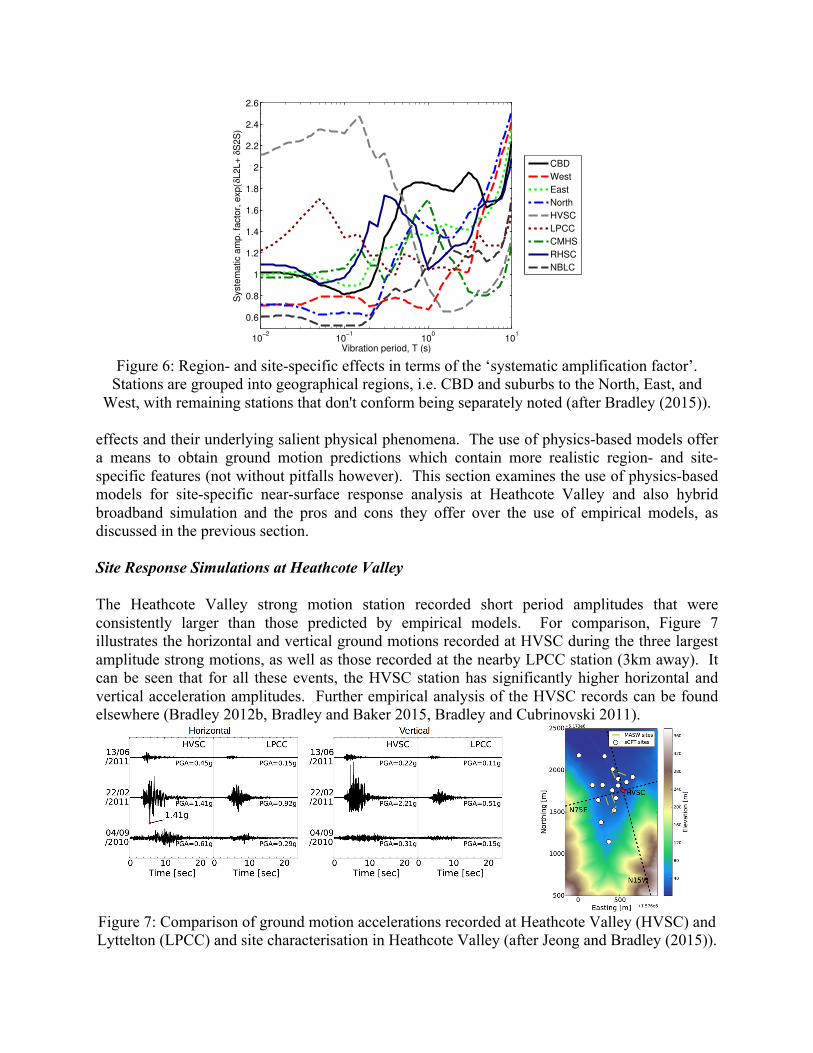
Figure 6: Region- and site-specific effects in terms of the ‘systematic amplification factor’.
Stations are grouped into geographical regions, i.e. CBD and suburbs to the North, East, and West, with remaining stations that don't conform being separately noted (after Bradley (2015)).
effects and their underlying salient physical phenomena. The use of physics-based models offer a means to obtain ground motion predictions which contain more realistic region- and site-specific features (not without pitfalls however). This section examines the use of physics-based models for site-specific near-surface response analysis at Heathcote Valley and also hybrid broadband simulation and the pros and cons they offer over the use of empirical models, as discussed in the previous section.
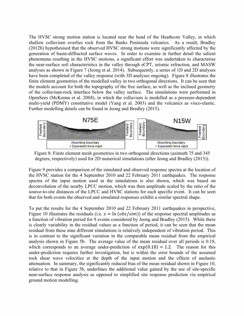
Site Response Simulations at Heathcote Valley The Heathcote Valley strong motion station recorded short period amplitudes that were consistently larger than those predicted by empirical models. For comparison, Figure 7 illustrates the horizontal and vertical ground motions recorded at HVSC during the three largest amplitude strong motions, as well as those recorded at the nearby LPCC station (3km away). It can be seen that for all these events, the HVSC station has significantly higher horizontal and vertical acceleration amplitudes. Further empirical analysis of the HVSC records can be found elsewhere (Bradley 2012b, Bradley and Baker 2015, Bradley and Cubrinovski 2011).
Figure 7: Comparison of ground motion accelerations recorded at Heathcote Valley (HVSC) and Lyttelton (LPCC) and site characterisation in Heathcote Valley (after Jeong and Bradley (2015)).
10−2
10−1
100
101
0.6
0.8
1
1.2
1.4
1.6
1.8
2
2.2
2.4
2.6
Vibration period, T (s)
Sys
tem
atic
am
p.
fact
or,
exp
( δL2
L+
δS
2S
)
CBD
West
East
North
HVSC
LPCC
CMHS
RHSC
NBLC
The HVSC strong motion station is located near the head of the Heathcote Valley, in which shallow colluvium overlies rock from the Banks Peninsula volcanics. As a result, Bradley (2012b) hypothesised that the observed HVSC strong motions were significantly affected by the generation of basin-diffracted surface waves. In order to examine in further detail the salient phenomena resulting in the HVSC motions, a significant effort was undertaken to characterise the near-surface soil characteristics in the valley through sCPT, seismic refraction, and MASW analyses as shown in Figure 7 (Jeong et al. 2014). Subsequently, a series of 1D and 2D analyses have been completed of the valley response (with 3D analyses ongoing). Figure 8 illustrates the finite element geometries of the modelled valley in two orthogonal directions. It can be seen that the models account for both the topography of the free surface, as well as the inclined geometry of the colluvium-rock interface below the valley surface. The simulations were performed in OpenSees (McKenna et al. 2004), in which the colluvium is modelled as a pressure-dependent multi-yield (PDMY) constitutive model (Yang et al. 2003) and the volcanics as visco-elastic. Further modelling details can be found in Jeong and Bradley (2015).
Figure 8: Finite element mesh geometries in two orthogonal directions (azimuth 75 and 345 degrees, respectively) used for 2D numerical simulations (after Jeong and Bradley (2015)).
Figure 9 provides a comparison of the simulated and observed response spectra at the location of the HVSC station for the 4 September 2010 and 22 February 2011 earthquakes. The response spectra of the input motion used in the simulations is also shown, which was based on deconvolution of the nearby LPCC motion, which was then amplitude scaled by the ratio of the source-to-site distances of the LPCC and HVSC stations for each specific event. It can be seen that for both events the observed and simulated responses exhibit a similar spectral shape.
To put the results for the 4 September 2010 and 22 February 2011 earthquakes in perspective, Figure 10 illustrates the residuals (i.e. 𝑧 = ln (𝑜𝑏𝑠/𝑠𝑖𝑚)) of the response spectral amplitudes as a function of vibration period for 9 events considered by Jeong and Bradley (2015). While there is clearly variability in the residual values as a function of period, it can be seen that the mean residual from these nine different simulations is relatively independent of vibration period. This is in contrast to the significant variation in the comparable mean residual from the empirical analysis shown in Figure 5b. The average value of the mean residual over all periods is 0.18, which corresponds to an average under-prediction of exp 0.18 = 1.2. The reason for this under-prediction requires further investigation, but is within the error bounds of the assumed rock shear wave velocities at the depth of the input motion and the effects of anelastic attenuation. In summary, the significantly reduced bias of the mean residual shown in Figure 10, relative to that in Figure 5b, underlines the additional value gained by the use of site-specific near-surface response analysis as opposed to simplified site response prediction via empirical ground motion modelling.

Figure 9: Comparison of simulated and observed ground motion response spectra at the HVSC station location, (azimuth 75 degrees) from the finite element model in Figure 8a, for the: (a) 4
September 2010; and (b) 22 February 2011 earthquakes.
Figure 10: Residuals (𝑧 = ln (𝑜𝑏𝑠/𝑠𝑖𝑚)) in predicting response spectral amplitudes at the
Heathcote Valley strong motion station (HVSC) for 9 events considered by Jeong and Bradley (2015).
Hybrid Broadband Simulations of the Canterbury Earthquakes Ground motion simulation based on a physical representation of the seismic source, a 3D model of the geophysical properties of the earth’s crust, and site-specific near-surface soil stratigraphy can provide significant physical insight into salient ground motion phenomena beyond that obtainable from a comparison of observations with empirical ground motion models. In this section, a summary of hybrid broadband ground motion simulation results based on the method of Graves and Pitarka (2015, 2010) is presented.
10−2
10−1
100
101
10−2
10−1
100
101
Period, T (s)
Sp
ect
ral a
cc,
SA
(g
)
Input motion (scaled LPCC)
Simulation
Observed (HVSC)
4 September 2010
10−2
10−1
100
101
10−2
10−1
100
101
Period, T (s)
Spect
ral a
cc, S
A (
g)
Input motion (scaled LPCC)
Simulation
Observed (HVSC)
22 February 2011
10−2
10−1
100
101
−2
−1.5
−1
−0.5
0
0.5
1
1.5
2
Period, T (s)
To
tal r
esi
du
al,
z =
ln(o
bs/
sim
)
Individual events
22 February 2011
4 September 2010
Mean
(a) (b)

Ground motion simulation was performed for the 10 previously noted events. The largest four events (4/09/2010, 22/2/2011, 13/06/2011, 23/12/2011) were modelled as kinematic finite faults, while the six smaller events are considered as point sources. The finite fault models are based on the source inversion geometries of Beavan et al. (2011, 2012, 2010). Three of these four ‘main’ earthquakes in the sequence are postulated to have occurred on multiple fault planes. For simplicity, only the 4 September 2010 Darfield earthquake is modelled with multiple fault planes, and the single fault geometries for the 22 February and 13 June earthquakes are considered. The source geometry and hypocentre of Beavan et al. are utilized, but the slip distribution is stochastic following Graves and Pitarka (2015, 2010).
The 3D representation of the shallow crust in the Canterbury region utilizes version 1.61 of the Canterbury Velocity Model (CantVM) (Bradley et al. 2015, Lee et al. 2015). This model utilizes data from travel time tomography, seismic reflection, petroleum and hydrologic wells, active and passive surface wave analysis, and seismic CPT. The model provides a detailed representation of the surface of the Torlesse basement rock and Banks Peninsula volcanics, which are the two large impedance surfaces which have a strong influence on seismic wave propagation in the region.
The Graves and Pitarka simulation method utilizes a hybrid approach in which ground motion at low frequencies is obtained from 3D wave propagation, and stochastic simulation at high frequencies. The low frequency simulation (f≤1Hz) solves the viscoelastic wave propagation problem using a kinematic representation of the rupture source and 3D heterogenous crustral structure based on a staggered-grid finite difference scheme with 4th and 2nd order accuracy in space and time. Anelastic attenuation is considered as a function of shear wave velocity: 𝑄! = 100𝑉!;𝑄! = 50𝑉!. A minimum shear wave velocity of 500m/s; and a spatial grid spacing of 0.1km are utilized to enable an accurate simulation of frequencies up to 𝑓=1Hz. The high-frequency simulation (f≥1Hz) is based on a semi-empirical stochastic approach in a 1D velocity structure for the region (Bradley and Graves 2014) in which the following parameters were adopted: stress drop, 𝛥𝜎=4MPa; Anelastic attenuation, 𝑄 = 𝑄!𝑓!, where 𝑄! = 41+ 34𝑉! and 𝑥 = 0.6; and high frequency attenuation, 𝜅=0.045. In the presented results, local site effects are incorpated via the simplified empirical approach of Campbell and Bozorgnia (2008) as discussed in Graves and Pitarka (2010), although we are presently working to couple these broadband ground motion simulations with site-specific near-surface site response (such as that discussed in the previous section).
Figure 11 and Figure 12 provide illustrations of the simulated ground velocities during the 4 September 2010 Darfield and 22 February 2011 Christchurch earthquakes, respectively. In the 4 September 2010 event, the four images at time increments of 5 seconds clearly illustrate: the significant forward directivity effects that develop at the eastern and western edges of the rupturing faults (t=16s); the modification of the eastward propagating directivity pulse as it encounters the Banks Peninsula volcanic region leading to focusing to the North in Christchuch (t=21s); and the significant basin-induced surface waves which propagate through Christchurch city to the east, and bounded by the significant basin edge caused by the Hororata fault to the west (t=26 and 31s). The significance of directivity and basin-generated surface waves are also
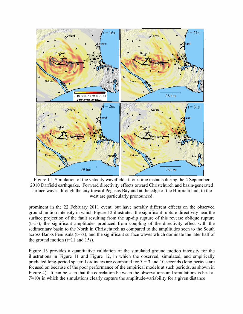
Figure 11: Simulation of the velocity wavefield at four time instants during the 4 September
2010 Darfield earthquake. Forward directivity effects toward Christchurch and basin-generated surface waves through the city toward Pegasus Bay and at the edge of the Hororata fault to the
west are particularly pronounced. prominent in the 22 February 2011 event, but have notably different effects on the observed ground motion intensity in which Figure 12 illustrates: the significant rupture directivity near the surface projection of the fault resulting from the up-dip rupture of this reverse oblique rupture (t=5s); the significant amplitudes produced from coupling of the directivity effect with the sedimentary basin to the North in Christchurch as compared to the amplitudes seen to the South across Banks Peninsula (t=8s); and the significant surface waves which dominate the later half of the ground motion (t=11 and 15s).
Figure 13 provides a quantitative validation of the simulated ground motion intensity for the illustrations in Figure 11 and Figure 12, in which the observed, simulated, and empirically predicted long-period spectral ordinates are compared for T = 3 and 10 seconds (long periods are focused on because of the poor performance of the empirical models at such periods, as shown in Figure 4). It can be seen that the correlation between the observations and simulations is best at T=10s in which the simulations clearly capture the amplitude-variability for a given distance
t = 16s
t = 31s
t = 21s
t = 26s

Figure 12: Simulation of the velocity wavefield at four time instants during the 22 February 2011 Christchurch earthquake. The directivity-basin coupling leads to significantly greater motions in
the city to the north of the fault than those at similar distances in other directions. seen in the observations, and amplitudes that are, on average, larger than the median empirical prediction. It can also been seen in the T = 3s ordinates that the simulations capture the large observed ground motion amplitudes in Christchurch (for which 𝑅!"#=15-20km and 2-8km in the Darfield and Christchurch events, respectively) resulting from directivity-basin coupling. The slight systematic over-prediction of the simulations for T = 3 seconds is postulated as a result of neglecting a weathered layer in the current representation of the Banks Peninsula volcanics in the v1.61 CantVM velocity model utilized – which is being currently explored. Figure 14 provides a summary of the performance of the hybrid broadband ground motion simulation (based on the v1.61 CantVM velocity model) across the 10 considered earthquake events via the between-event residuals, i.e. the mean of ln (𝑜𝑏𝑠/𝑠𝑖𝑚) across all of the strong motion stations. It can be seen that for 7 of the 10 events, the simulations generally over-predict the observed spectral amplitudes for periods in the range of T=1-5s, which is inferred as a result of an excessive impedance contrast to the Banks Peninsula volcanics (as noted previously). In contrast, for three of the 10 events (13 June 2011, and two events on 23 December 2011) there is
t = 5s
t = 11s t = 16s
t = 8s

Figure 13: Comparison of long-period (T = 3, 10s) pseudo-acceleration response spectral
amplitudes observed during the 4 September 2010 (left) and 22 February 2011 (right) earthquakes. Geometric mean observations and simulations at strong motion station locations
are shown as points; as well as the median, 16th and 84th percentiles of the NZ-specific empirical model of Bradley (2013).
a general under-prediction of the observations, even at short vibration periods. The 13 June and 23 December Mw5.9 earthquakes are two of four events that are modelled as finite faults, and it is recognied that the quality of the adopted finite fault models is significantly less than the more well studied ruptures for the 4 September 2010 and 22 February 2011 earthquakes. Clearly further research is needed to resolve the apparent issues for these events (which are also present in comparisons with empirical predictions).
Conclusions
This paper has examined the predictive capabilities of empirical and physics-based ground motion models for 10 events in the 2010-2011 Canterbury earthquake sequence. The repeated recordings at the same set of locations in the observed strong motion dataset allowed insight into both the average performance of models across all strong motion stations, as well as any systematic biases at specific locations. The Heathcote Valley strong motion station (HVSC) was one such location in which observed response spectral amplitudes were seen to be systematically
100
101
102
10−2
10−1
100
Source−to−site distance, R rup
(km)
Spect
ral a
ccele
ratio
n, S
A(3
s) (
g)
4 September 2010 Mw 7.1
ObsSimGMPE
100
101
102
10−3
10−2
10−1
100
Source−to−site distance, R rup
(km)
Sp
ect
ral a
ccele
ratio
n, S
A(3
s) (
g)
ObsSimGMPE
100
101
102
10−3
10−2
10−1
Source−to−site distance, R rup
(km)
Spect
ral a
ccele
ratio
n, S
A(1
0s)
(g)
ObsSimGMPE
100
101
102
10−4
10−3
10−2
10−1
Source−to−site distance, R rup
(km)
Spect
ral a
ccele
ratio
n, S
A(1
0s)
(g)
ObsSimGMPE
(a) (b)
(c) (d)
100
101
102
10−2
10−1
100
Source−to−site distance, R rup
(km)
Sp
ect
ral a
cce
lera
tion
, S
A(1
s) (
g)
22 February 2011 Mw 6.2
ObsSimGMPE
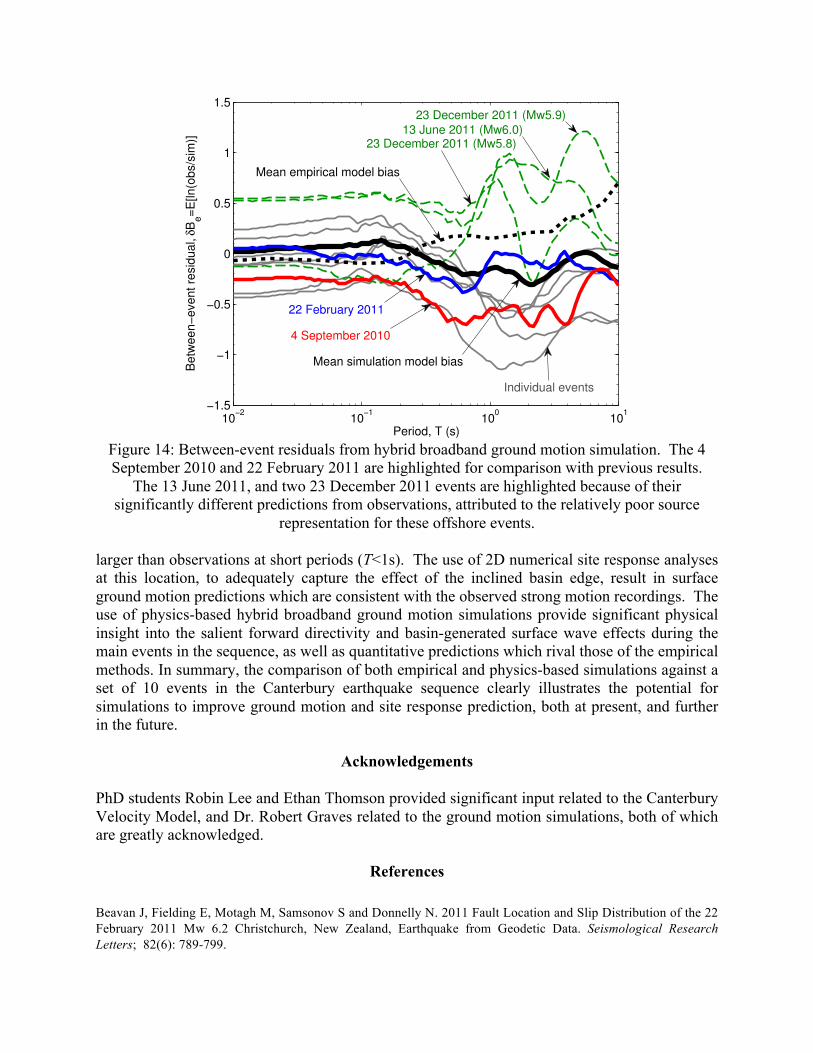
Figure 14: Between-event residuals from hybrid broadband ground motion simulation. The 4 September 2010 and 22 February 2011 are highlighted for comparison with previous results.
The 13 June 2011, and two 23 December 2011 events are highlighted because of their significantly different predictions from observations, attributed to the relatively poor source
representation for these offshore events. larger than observations at short periods (T<1s). The use of 2D numerical site response analyses at this location, to adequately capture the effect of the inclined basin edge, result in surface ground motion predictions which are consistent with the observed strong motion recordings. The use of physics-based hybrid broadband ground motion simulations provide significant physical insight into the salient forward directivity and basin-generated surface wave effects during the main events in the sequence, as well as quantitative predictions which rival those of the empirical methods. In summary, the comparison of both empirical and physics-based simulations against a set of 10 events in the Canterbury earthquake sequence clearly illustrates the potential for simulations to improve ground motion and site response prediction, both at present, and further in the future.
Acknowledgements
PhD students Robin Lee and Ethan Thomson provided significant input related to the Canterbury Velocity Model, and Dr. Robert Graves related to the ground motion simulations, both of which are greatly acknowledged.
References
Beavan J, Fielding E, Motagh M, Samsonov S and Donnelly N. 2011 Fault Location and Slip Distribution of the 22 February 2011 Mw 6.2 Christchurch, New Zealand, Earthquake from Geodetic Data. Seismological Research Letters; 82(6): 789-799.
10−2
10−1
100
101
−1.5
−1
−0.5
0
0.5
1
1.5
Period, T (s)
Betw
een−
eve
nt re
sidual,
δB
e=
E[ln
(obs/
sim
)]
22 February 2011
4 September 2010
Mean simulation model bias
Individual events
23 December 2011 (Mw5.9)13 June 2011 (Mw6.0)
23 December 2011 (Mw5.8)
Mean empirical model bias

Beavan J, Motagh M, Fielding EJ, Donnelly N and Collett D. 2012 Fault slip models of the 2010–2011 Canterbury, New Zealand, earthquakes from geodetic data and observations of postseismic ground deformation. New Zealand Journal of Geology and Geophysics; 55(3): 207-221.
Beavan J, Samsonov S, Motagh M, Wallace L, Ellis S and Palmer N. 2010 The Darfield (Canterbury) Earthquake: Geodetic observations and preliminary source model. Bulletin of the New Zealand Society for Earthquake Engineering; 43(4): 228-235.
Berrill JB, Avery H, Dewe M, Chanerley AA, Alexander NN, Dyer C, Holden C and Fry B. 2011 The Canterbury Accelerograph Network (CanNet) and some results from the September 2010, M7.1 Darfield Earthquake, in 9th Pacific Conference on Earthquake Engineering: Auckland, New Zealand, 8.
Bradley BA. 2012a Ground motions observed in the Darfield and Christchurch earthquakes and the importance of local site response effects. New Zealand Journal of Geology and Geophysics; 55(3): 279-286.
Bradley BA. 2012b Strong ground motion characteristics observed in the 4 September 2010 Darfield, New Zealand earthquake. Soil Dynamics and Earthquake Engineering; 42 32-46.
Bradley BA. 2013 A New Zealand-Specific Pseudospectral Acceleration Ground-Motion Prediction Equation for Active Shallow Crustal Earthquakes Based on Foreign Models. Bulletin of the Seismological Society of America; 103(3): 1801-1822.
Bradley BA. 2015 Systematic ground motion observations in the Canterbury earthquakes and region-specific non-ergodic empirical ground motion modeling. Earthquake Spectra; (in press).
Bradley BA and Baker JW. 2015 Ground motion directionality in the 2010–2011 Canterbury earthquakes. Earthquake Engineering & Structural Dynamics; 44(3): 371-384.
Bradley BA and Cubrinovski M. 2011 Near-source Strong Ground Motions Observed in the 22 February 2011 Christchurch Earthquake. Seismological Research Letters; 82(6): 853-865.
Bradley BA and Graves RW. 2014 Low frequency (f≤1Hz) ground motion simulations of 10 events in the 2010-2011 Canterbury earthquake sequence, in Southern California Earthquake Centre (SCEC) Annual Meeting: Palm Springs, California.
Bradley BA, Lee RL, Thomson EM, Ghisetti F, McGann C, Pettinga JR and Hughes MW. 2015 3D Canterbury Velocity Model (CantVM) - Version 1.0, in Southern California Earthquake Center (SCEC) Annual Meeting: Palm Springs, CA.
Bradley BA, Quigley MC, Van Dissen RJ and Litchfield NJ. 2014 Ground Motion and Seismic Source Aspects of the Canterbury Earthquake Sequence. Earthquake Spectra; 30(1): 1-15.
Buchanan A, Carradine D, Beattie GJ and Morris H. 2011 Performance of houses during the Christchurch earthquake of 22 February 2011. Bulletin of the New Zealand Society for Earthquake Engineering; 44(4): 342-357.
Campbell KW and Bozorgnia Y. 2008 NGA Ground Motion Model for the Geometric Mean Horizontal Component of PGA, PGV, PGD and 5% Damped Linear Elastic Response Spectra for Periods Ranging from 0.01 to 10 s. Earthquake Spectra; 24(1): 139-171.
Clifton C, Bruneau M, MacRae GA, Leon RT and Fussell A. 2011 Steel Structures Damage from the Christchurch Earthquake Series of 2010 and 2011. Bulletin of the New Zealand Society for Earthquake Engineering; 44(4): 297-318.
Cubrinovski M, Bradley BA, Wotherspoon L, Green AG, Bray J, Wood C, Pender M, Allen CR, Bradshaw A, Rix G, Taylor M, Robinson K, Henderson D, Giorgini S, Ma K, Winkley A, Zupan J, O'Rourke TD, DePascale G and Wells DL. 2011 Geotechnical Aspects of the 22 February 2011 Christchurch Earthquake. Bulletin of the New Zealand Society for Earthquake Engineering; 44(4): 205-226.
Gledhill K, Ristau J, Reyners M, Fry B and Holden C. 2011 The Darfield (Canterbury, New Zealand) Mw 7.1 Earthquake of September 2010: A Preliminary Seismological Report. Seismological Research Letters; 82(3): 378-386.

Graves R and Pitarka A. 2015 Refinements to the Graves and Pitarka (2010) Broadband Ground-‐‑Motion Simulation Method. Seismological Research Letters; 86(1): 75-80.
Graves RW and Pitarka A. 2010 Broadband Ground-Motion Simulation Using a Hybrid Approach. Bulletin of the Seismological Society of America; 100(5A): 2095-2123.
Jeong S and Bradley BA. 2015 Simulation of 2D site response at Heathcote Valley during the 2010-2011 Canterbury earthquake sequence, in 10th Pacific Conference on Earthquake Engineering: Sydney, Australia, 8.
Jeong S, Bradley BA, McGann CR and DePascale G. 2014 Characterization of dynamic soil properties and stratigraphy at Heathcote Valley, New Zealand, for simulation of 3D valley effects, in Southern California Earthquake Centre (SCEC) Annual Meeting: Palm Springs, California.
Kaiser A, Holden C, Beavan J, Beetham D, Benites R, Celentano A, Collett D, Cousins J, Cubrinovski M, Dellow G, Denys P, Fielding E, Fry B, Gerstenberger M, Langridge R, Massey C, Motagh M, Pondard N, McVerry G, Ristau J, Stirling M, Thomas J, Uma SR and Zhao J. 2012 The Mw 6.2 Christchurch earthquake of February 2011: preliminary report. New Zealand Journal of Geology and Geophysics; 55(1): 67-90.
Kam WY, Pampanin S and Elwood KJ. 2011 Seismic performance of reinforced concrete buidlings in the 22 Febraury Christchurch (Lyttelton) Earthquake. Bulletin of the New Zealand Society for Earthquake Engineering; 44(4): 239-278.
Lee RL, Bradley BA, Ghisetti F, Thomson EM, Pettinga JR and Hughes MW. 2015 A geology-based 3D seismic velocity model of Canterbury, New Zealand, in New Zealand Society for Earthquake Engineering (NZSEE) Annual Conference: Rotorua, 8.
Massey CI, McSaveney MJ, Taig T, Richards L, Litchfield NJ, Rhoades DA, McVerry GH, Lukovic B, Heron DW, Ries W and Van Dissen RJ. 2014 Determining Rockfall Risk in Christchurch Using Rockfalls Triggered by the 2010–2011 Canterbury Earthquake Sequence. Earthquake Spectra; 30(1): 155-181.
McKenna F, Fenves GL and Scott MH. 2004 OpenSees: Open system for earthquake engineering simulation. Pacific Earthquake Engineering Research Center, University of California, Berkeley, CA.
Quigley MC, Bastin S and Bradley BA. 2013 Recurrent liquefaction in Christchurch, New Zealand, during the Canterbury earthquake sequence. Geology; 41(4): 419-422.
Yang Z, Elgamal AW and Parra E. 2003 Computational model for cyclic mobility and associated shear deformation. Journal of Geotechnical and Geoenvironmental Engineering; 129(12): 1119-1127.