Validation of NOAA CPC RFE Satellite-based Rainfall ...lib.icimod.org/record/28331/files/WP_13-5.pdf · Validation of NOAA CPC_RFE Satellite-based Rainfall Estimates in the Central

1

ICIMOD Working Paper 2013/5

Validation of NOAA CPC_RFE Satellite-based Rainfall Estimates in the Central Himalayas

About ICIMOD

The International Centre for Integrated Mountain Development, ICIMOD, is a regional knowledge

development and learning centre serving the eight regional member countries of the Hindu Kush

Himalayas – Afghanistan, Bangladesh, Bhutan, China, India, Myanmar, Nepal, and Pakistan – and

based in Kathmandu, Nepal. Globalization and climate change have an increasing influence on

the stability of fragile mountain ecosystems and the livelihoods of mountain people. ICIMOD aims

to assist mountain people to understand these changes, adapt to them, and make the most of new

opportunities, while addressing upstream-downstream issues. We support regional transboundary

programmes through partnership with regional partner institutions, facilitate the exchange of

experience, and serve as a regional knowledge hub. We strengthen networking among regional

and global centres of excellence. Overall, we are working to develop an economically and

environmentally sound mountain ecosystem to improve the living standards of mountain populations

and to sustain vital ecosystem services for the billions of people living downstream – now, and for

the future.

ICIMOD gratefully acknowledges the support of its core donors: the Governments of Afghanistan,

Bangladesh, Bhutan, China, India, Myanmar, Nepal, Pakistan, Austria, Norway, Switzerland, and

the United Kingdom.

i

Validation of NOAA CPC_RFE Satellite-based Rainfall Estimates in the Central Himalayas

ICIMOD Working Paper 2013/5

Mandira Singh ShresthaRupak RajbhandariSagar Ratna Bajracharya

International Centre for Integrated Mountain Development, Kathmandu, Nepal, May 2013

ii

Copyright © 2013International Centre for Integrated Mountain Development (ICIMOD)All rights reserved.

Published byInternational Centre for Integrated Mountain DevelopmentGPO Box 3226, Kathmandu, Nepal

ISBN 978 92 9115 283 4 (printed)

978 92 9115 284 1 (electronic)

Production TeamA. Beatrice Murray (Consultant editor); Amy Sellmyer (Editor); Dharma R Maharjan (Layout and design); Asha Kaji Thaku (Editorial assistant)

Printed by Quality Printers (P) Ltd, Kathmandu, Nepal

ReproductionThis publication may be reproduced in whole or in part and in any form for educational or non-profit purposes without special permission from the copyright holder, provided acknowledgement of the source is made. ICIMOD would appreciate receiving a copy of any publication that uses this publication as a source.

No use of this publication may be made for resale or for any other commercial purpose whatsoever without prior permission in writing from ICIMOD.

NoteThe views and interpretations in this publication are those of the authors. They are not attributable to ICIMOD.

This publication is also available at www.icimod.org/publications

Citation: Shrestha, MS; Rajbhandari, R; Bajracharya, SR (2013) Validation of NOAA CPC_RFE satellite-based rainfall estimates in the central Himalayas. ICIMOD Working Paper 2013/5. Kathmandu: ICIMOD

iii

ContentsForeword viAcknowledgements viiAcronyms and Abbreviations viII

Introduction 1 Background 1 ICIMOD Satellite Rainfall Estimation Project 1 Present Study 2

Study Region and Data 3 Study Region 3 Data Availability 3

Methodology for Rainfall Verification 5 Interpolation of Gauge-Observed Rainfall 5 Rainfall Verification Methodology 6 Visual Analysis 6 Continuous Verification Statistics 6 Categorical Verification Statistics 6

Analysis and Results 8 Comparison of Quantitative Rainfall Distribution 8 Comparision of Spatial Distribution of Rainfall as Estimated from CPC_RFE2.0 and Gauge-Observed Data 13 Monthly Bias Map Preparation and Analysis 14 Error Statistics for Satellite-Based Rainfall Estimates 17

Discussion and Conclusion 21 Satellite-Estimated Values 21 Improving Values 21 Conclusion 24

References 25

Annex: Rain Gauge Stations 27

iv

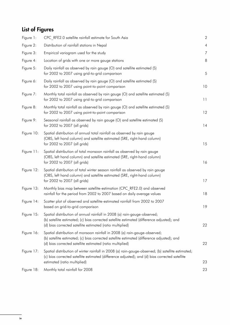
List of FiguresFigure 1: CPC_RFE2.0 satellite rainfall estimate for South Asia 2

Figure 2: Distribution of rainfall stations in Nepal 4

Figure 3: Empirical variogram used for the study 7

Figure 4: Location of grids with one or more gauge stations 8

Figure 5: Daily rainfall as observed by rain gauge (O) and satellite estimated (S) for 2002 to 2007 using grid-to-grid comparison 5

Figure 6: Daily rainfall as observed by rain gauge (O) and satellite estimated (S) for 2002 to 2007 using point-to-point comparison 10

Figure 7: Monthly total rainfall as observed by rain gauge (O) and satellite estimated (S) for 2002 to 2007 using grid-to-grid comparison 11

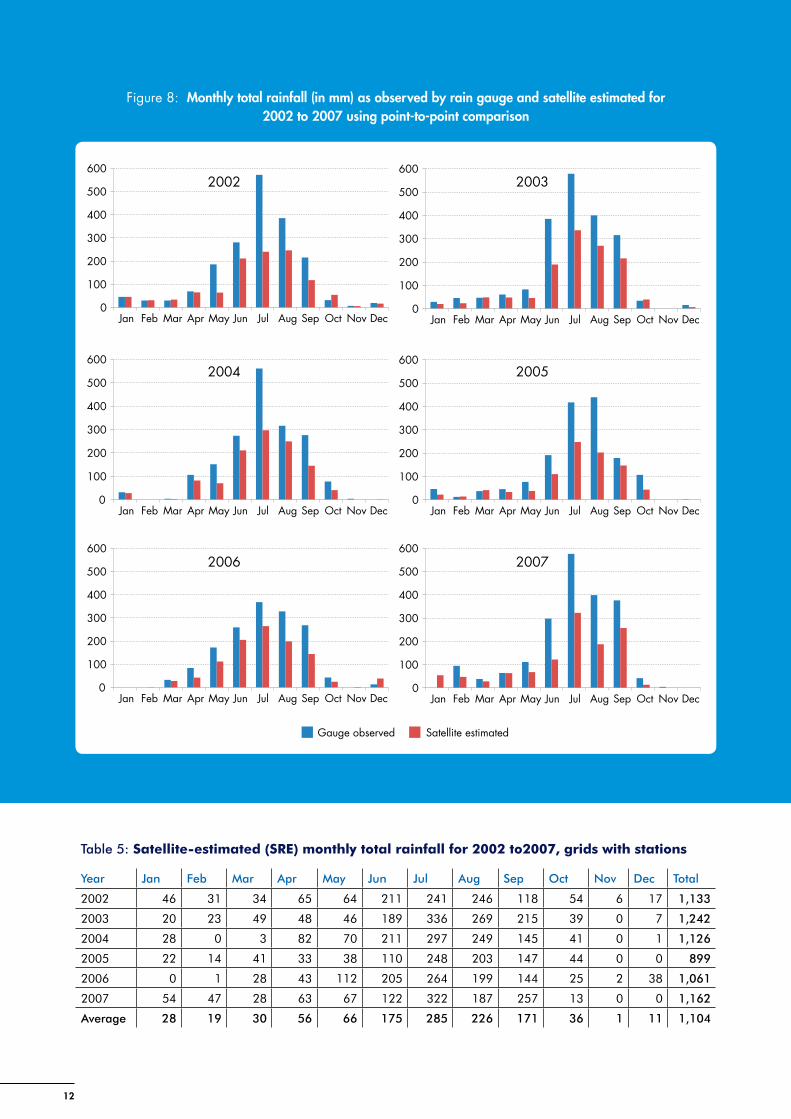
Figure 8: Monthly total rainfall as observed by rain gauge (O) and satellite estimated (S) for 2002 to 2007 using point-to-point comparison 12

Figure 9: Seasonal rainfall as observed by rain gauge (O) and satellite estimated (S) for 2002 to 2007 (all grids) 14

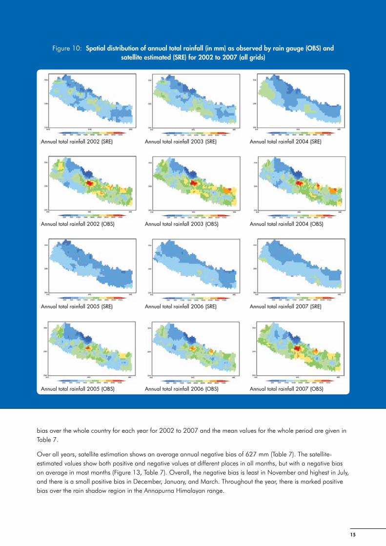
Figure 10: Spatial distribution of annual total rainfall as observed by rain gauge (OBS, left hand column) and satellite estimated (SRE, right-hand column) for 2002 to 2007 (all grids) 15

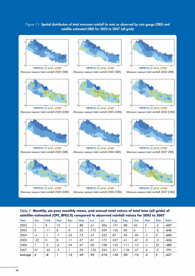
Figure 11: Spatial distribution of total monsoon rainfall as observed by rain gauge (OBS, left hand column) and satellite estimated (SRE, right-hand column) for 2002 to 2007 (all grids) 16

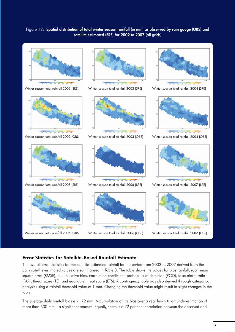
Figure 12: Spatial distribution of total winter season rainfall as observed by rain gauge (OBS, left hand column) and satellite estimated (SRE, right-hand column) for 2002 to 2007 (all grids) 17

Figure 13: Monthly bias map between satellite-estimation (CPC_RFE2.0) and observed rainfall for the period from 2002 to 2007 based on daily average values 18

Figure 14: Scatter plot of observed and satellite-estimated rainfall from 2002 to 2007 based on grid-to-grid comparison 19

Figure 15: Spatial distribution of annual rainfall in 2008 (a) rain-gauge-observed; (b) satellite estimated; (c) bias corrected satellite estimated (difference adjusted); and (d) bias corrected satellite estimated (ratio multiplied) 22

Figure 16: Spatial distribution of monsoon rainfall in 2008 (a) rain-gauge-observed; (b) satellite estimated; (c) bias corrected satellite estimated (difference adjusted); and (d) bias corrected satellite estimated (ratio multiplied) 22

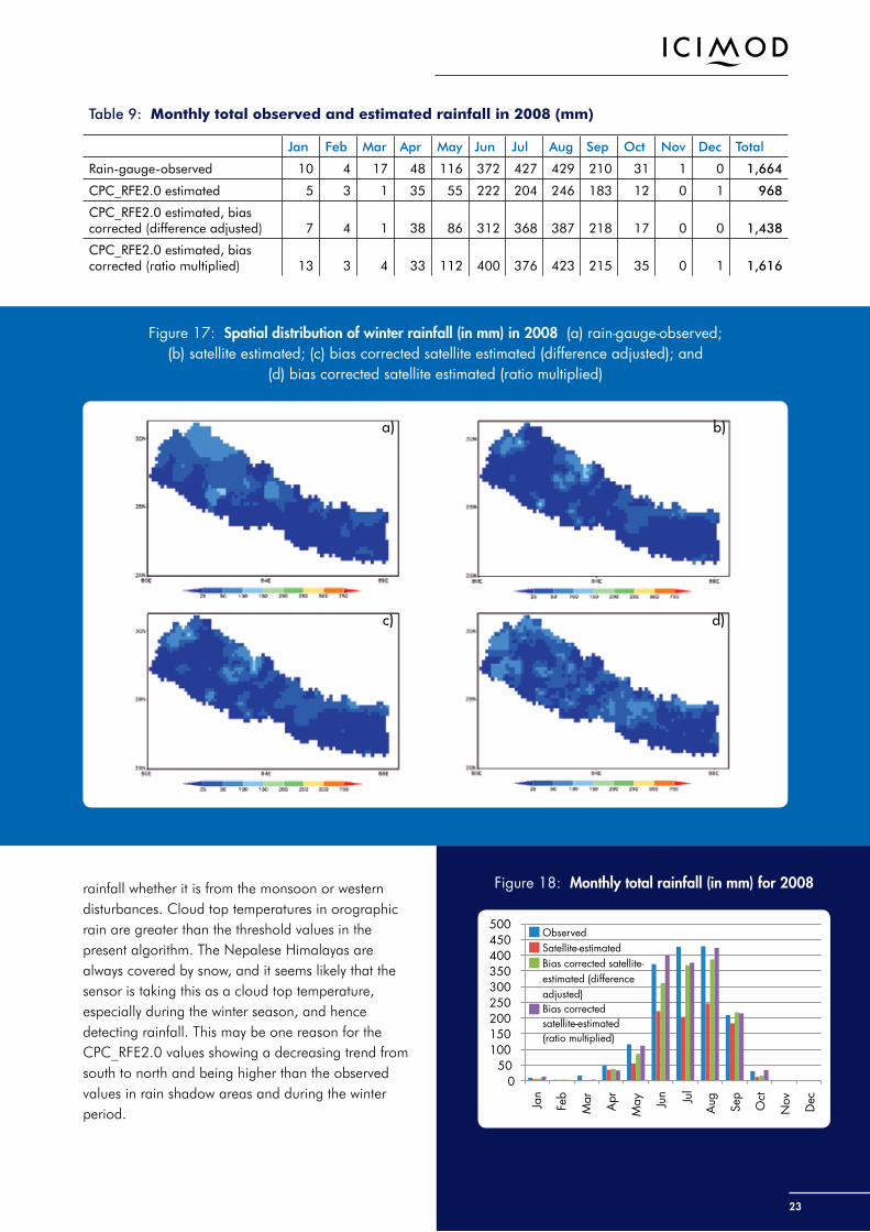
Figure 17: Spatial distribution of winter rainfall in 2008 (a) rain-gauge-observed; (b) satellite estimated; (c) bias corrected satellite estimated (difference adjusted); and (d) bias corrected satellite estimated (ratio multiplied) 23

Figure 18: Monthly total rainfall for 2008 23

v

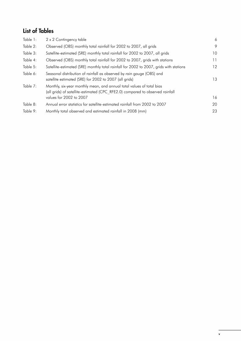
List of TablesTable 1: 2 x 2 Contingency table 6

Table 2: Observed (OBS) monthly total rainfall for 2002 to 2007, all grids 9

Table 3: Satellite-estimated (SRE) monthly total rainfall for 2002 to 2007, all grids 10

Table 4: Observed (OBS) monthly total rainfall for 2002 to 2007, grids with stations 11

Table 5: Satellite-estimated (SRE) monthly total rainfall for 2002 to 2007, grids with stations 12

Table 6: Seasonal distribution of rainfall as observed by rain gauge (OBS) and satellite estimated (SRE) for 2002 to 2007 (all grids) 13

Table 7: Monthly, six-year monthly mean, and annual total values of total bias (all grids) of satellite-estimated (CPC_RFE2.0) compared to observed rainfall values for 2002 to 2007 16

Table 8: Annual error statistics for satellite-estimated rainfall from 2002 to 2007 20

Table 9: Monthly total observed and estimated rainfall in 2008 (mm) 23

vi

Foreword

The Hindu Kush Himalayan region is vulnerable to many types of natural hazard, and especially to floods and landslides. Annually, thousands of lives are lost, infrastructure worth millions of dollars is destroyed, and large numbers of people are rendered homeless by floods. It is difficult to reduce the actual occurrence of floods, but the damage and adverse impacts can be averted or minimized with adequate warning. In order to prepare timely and accurate flood warnings, however, it is necessary to have good information about rainfall. The main method used to estimate rainfall is interpolation of measurements from a network of hydrometeorological stations. However, the number of hydrometeorological stations in the high mountain areas of the Hindu Kush Himalayas is limited as a result of the steep terrain and poor accessibility, and there is little information available about rainfall in the upper catchments of the flood-prone rivers. Advances in technology and the availability of satellite-based rainfall estimates provide an opportunity to supplement gauge-observed data with estimates and provide early warning to the people at risk in this otherwise data sparse region.

Since 2006, the International Centre for Integrated Mountain Development (ICIMOD) has been working to assess the accuracy and test the applicability of satellite-based rainfall estimates in the Hindu Kush Himalayan region in collaboration with regional partners and with technical support from the National Oceanic and Atmospheric Administration (NOAA) and United States Geological Survey (USGS) and financial support from United States Agency for International Development Office of Foreign Disaster Assistance (USAID/OFDA). In 2008, ICIMOD published the results of preliminary tests of the accuracy of rainfall estimates over the region. This publication presents the findings of a detailed assessment of the accuracy of CPC_RFE2.0 rainfall estimates over the central Himalayas of Nepal. The results indicate that the spatial detection and trends are overall good, and with appropriate bias correction, the data could be applied in flood forecasting.

Reducing vulnerability and building the resilience of communities in the region to extreme weather events remains a priority for ICIMOD as it embarks on its Medium Term Action Plan for 2013-2017. ICIMOD and its partners are committed to work together on disaster risk reduction and minimize the adverse impacts of disasters. We hope that this publication will contribute further to this work.

David Molden Director General, ICIMOD

vii

AcknowledgementsICIMOD is grateful to the United States Agency for International Development Office of Foreign Disaster Assistance (USAID/OFDA) for funding this project. Our special thanks go to A Sezin Tokar, Hydrometeorological Hazard Advisor, USAID/OFDA, for her encouragement and valuable support during the study. We would like to express our gratitude to the resource people from the National Oceanic and Atmospheric Administration (NOAA) and United States Geological Survey (USGS) for their technical support, in particularly Wassila Thiaw, Vadlamani B. Kumar, Eric Wolvovsky, Tim Love, and Guleid Artan. We thank the Department of Hydrology and Meteorology (DHM) Nepal for providing the data for the study and for their valuable contributions. Finally, the authors would like to thank all those in ICIMOD who contributed to the success of the project and the preparation of the publication itself.

viii

Acronyms and Abbreviations

AFN Asian Flood Network

AMSU-B Advanced Microwave Soundin Unit

DHM Department of Hydrology and Meteorology

ETS equitable threat score

FAR false alarm ratio

GeoSFM Geospatial Streamflow Model

GPI Geostationary Operational Environmental Satellite Precipitation Index

GSMaP Global Satellite Mapping Precipitation

GTS Global Telecommunications System (WMO)

HKH Hindu Kush Himalayan region

IR infrared

MAE mean absolute error

NOAA National Oceanic and Atmospheric Administration

OFDA Office of Foreign Disaster Assistance

PE percentage error

POD probability of detection

RSME root mean square error

SRE satellite rainfall estimates

SSMI spcial sensor microwave imager

USAID United States Agency for International Development

USGS United States Geological Survey

WMO World Meteorological Organization

1

Introduction

BackgroundFlood early warning systems are one of the most effective ways to minimize the loss of life and property. It is very important to have a reliable flood forecasting system as a basis for establishing a reliable early warning system which can be transmitted down to the community in order to minimize the impact of flood disasters. Precipitation is highly variable in both space and time and is an important input in rainfall runoff modelling. The amount of rainfall and its spatial distribution are important factors in meteorology, climatology, and hydrology. Accurate rainfall estimations are essential for timely flood forecasting and warning. In many regions, operational flood forecasting has traditionally relied upon a dense network of rain gauges or ground-based rainfall measuring radars that report in real time. Flood forecasting in basins with sparse or non-existent rain gauges poses an additional challenge. In such areas, satellite rainfall estimates (SRE) could provide information on rainfall occurrence, amount, and distribution (Adler et al. 2003; Hong et al. 2007; Shrestha et al. 2008 a,b) and be used for hydrological modelling to predict floods.

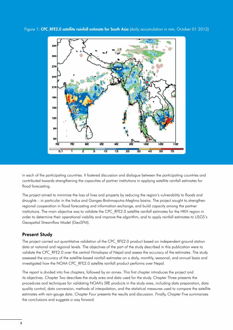
The availability of global coverage of satellite data offers an effective and economical means of calculating areal rainfall estimates in sparsely gauged areas (Artan et al. 2007). Several high resolution global satellite-based rainfall products are currently available from various operational agencies, as well from research and academic institutions (Ebert et al. 2007; Huffman et al. 2007; Kubota et al. 2009). For example, satellite algorithms like the Global Satellite Mapping Precipitation (GSMaP) (Ushio et al. 2009), CPC_RFE2.0 (Xie et al. 2002), and CMORPH (Joyce et al. 2004) are currently available at a spatial resolution of 0.1 degrees or higher and a temporal resolution of 24 hours or less. The availability of high resolution satellite-based products at a finer temporal (hourly and daily) and spatial (0.1°) resolution provides an opportunity to apply rainfall estimates for timely flood forecasts in data sparse regions. However, satellite-based rainfall data have uncertainty and, when applied in rainfall runoff models for flood simulation, this uncertainty has an effect on the accuracy of the predictions. Thus the satellite rainfall estimates need to be validated against rain gauge measurements to gain an idea of their accuracy and expected error characteristics in various applications before they can be used in modelling. Figure 1 shows an example of a daily satellite-based rainfall estimate for the Hindu Kush Himalayan (HKH) region provided by the National Oceanic and Atmospheric Administration (NOAA) Climate Prediction Centre (CPC) CPC_RFE2.0 (www.cpc.ncep.noaa.gov/products/fews/SASIA/rfe.shtml).

Following the successful validation of satellite rainfall estimates for regions in Africa, and similar estimates made over other parts of the world (Kidd 2005; Laurent et al. 1998; Vila et al. 2003; Dinku et al. 2008), the CPC_RFE2.0 system is now being tested in South Asia (Shrestha et al. 2008 a,b). The present study focuses on the verification of rainfall by CPC_RFE2.0 satellite-based rainfall estimates over the whole of Nepal.

The ICIMOD Satellite Rainfall Estimation ProjectICIMOD has collaborated with regional partner countries since 2001 on flood disaster mitigation, with support from the United States Agency for International Development Office of Foreign Disaster Assistance (USAID/OFDA). ICIMOD shared 24-hour, 48-hour, and 72-hour rainfall forecasts made available by OFDA for the HKH region with all its partners during the monsoon of 2004. Partners’ interest and requests led to a long-term project ‘Application of Satellite Rainfall Estimates in the Hindu Kush Himalayan Region’ on satellite rainfall verification and application. As part of the project, a series of trainings and workshops were held under the Asia Flood Network (AFN) programme of USAID/OFDA with technical support from NOAA and the United States Geological Survey (USGS).

Phase I of the project ended in June 2008, and Phase II, which continued the validation of the satellite-based rainfall estimates over the Himalayan region, ended in June 2010. The project engaged government representatives of national hydrological and meteorological services, and organizations involved in flood disaster management,

2

in each of the participating countries. It fostered discussion and dialogue between the participating countries and contributed towards strengthening the capacities of partner institutions in applying satellite rainfall estimates for flood forecasting.

The project aimed to minimize the loss of lives and property by reducing the region’s vulnerability to floods and droughts – in particular in the Indus and Ganges-Brahmaputra-Meghna basins. The project sought to strengthen regional cooperation in flood forecasting and information exchange, and build capacity among the partner institutions. The main objective was to validate the CPC_RFE2.0 satellite rainfall estimates for the HKH region in order to determine their operational viability and improve the algorithm, and to apply rainfall estimates to USGS’s Geospatial Streamflow Model (GeoSFM).

Present StudyThe project carried out quantitative validation of the CPC_RFE2.0 product based on independent ground station data at national and regional levels. The objectives of the part of the study described in this publication were to validate the CPC_RFE2.0 over the central Himalayas of Nepal and assess the accuracy of the estimates. The study assessed the accuracy of the satellite-based rainfall estimates on a daily, monthly, seasonal, and annual basis and investigated how the NOAA CPC_RFE2.0 satellite rainfall product performs over Nepal.

The report is divided into five chapters, followed by an annex. This first chapter introduces the project and its objectives. Chapter Two describes the study area and data used for the study. Chapter Three presents the procedures and techniques for validating NOAA’s SRE products in the study area, including data preparation, data quality control, data conversion, methods of interpolation, and the statistical measures used to compare the satellite estimates with rain-gauge data. Chapter Four presents the results and discussion. Finally, Chapter Five summarizes the conclusions and suggests a way forward.

Figure 1: CPC_RFE2.0 satellite rainfall estimate for South Asia (daily accumulation in mm, October 01 2012)

3

Study Region and Data

Study RegionNepal is a predominantly mountainous country with a total area of 147,181 km2 covering five physiographic regions: the Terai, Siwalik, Middle Mountains, High Mountains, and Himal. The elevation varies from 60 m in the south to 8,848 m in the north within a short horizontal distance of less than 200 km. Water-induced disasters are very prevalent and annually many lives are lost and property worth millions of dollars is destroyed. Due to the diverse geological setting, rugged terrain, and monsoon precipitation, Nepal is prone to floods, landslides, and glacial lake outburst floods (GLOF). The dominant rainfall season is the monsoon, which runs from June to September; 80 per cent of the annual rainfall falls during this period. The UNDP global report on reducing disaster risk (UNDP 2004) cites Nepal as having a high vulnerability for flood disasters based on 20 years of data (1980-2000). Between 1983 and 2005, an average of 309 people lost their lives annually in Nepal due to floods and landslides, accounting for over 60 per cent of those who died due to different types of disasters in the country (Khanal et al. 2007). The high level of poverty and rate of population growth has further increased the vulnerability to flood disasters.

Nepal has relatively few ground-based rain gauges, on average one gauge per 331 km2,according to the Department of Hydrology and Meteorology (DHM), with very few in the mountainous areas. Due to the limited spatial coverage of ground based gauges, lack of real-time rainfall data, and constraints in technical and financial resources, operational flood forecasting has yet to be initiated (Shrestha et al. 2008a). SRE may be an appropriate approach for Nepal to predict and forecast rainfall-induced runoff that may produce flooding.

Data Availability

NOAA CPC_RFE2.0 rainfall estimatesThe Climate Prediction Center (CPC) of NOAA has produced daily precipitation estimates (CPC_RFE2.0) on a 0.1 degree latitude/longitude grid over the HKH region (60°E-110°E; 5°N-40°N) in near real-time, at a spatial resolution of 0.1° by 0.1° (Xie et al. 2002) since 2001. The initial version, CPC_RFE1.0, was operational from 1996 to 2000 over Africa. The input data used for the operational rainfall estimates are from a combination of satellite estimates and rain gauges that use the algorithm developed by Xie and Arkin (1996). The satellite input data are from three sources: Advanced Microwave Sounding Unit (AMSU-B) microwave satellite precipitation estimates up to four times per day; Special Sensor Microwave Imager (SSMI) satellite rainfall estimates up to four times per day; and Geostationary Operational Environmental Satellite Precipitation Index (GPI) cloud-top infrared (IR) temperature precipitation estimates on a half-hourly basis. The rain gauge data are from the Global Telecommunications System (GTS) of the WMO. The three satellite estimates are first combined linearly using predetermined weighting coefficients then merged with station data to determine the final rainfall. The shape of the precipitation is given by the combined satellite estimates, and the magnitude is inferred from GTS station data. The merging technique using satellite-based rainfall data and ground gauge data increases the accuracy of the rainfall estimates by reducing significant bias and random error compared to individual data sources. Before these estimates can be used in modelling, however, they must be tested and optimized to ensure that they really reflect the situation on the ground. This system has produced an automatic rainfall analysis in South Asia since May 2001. Six years (2002 to 2007) of 24-hour CPC_RFE2.0 gridded rainfall data of 0.1° by 0.1° were obtained over the HKH region.

Gauge-observed rainfallThe daily gauge-observed rainfall data for the period 2002 to 2007 from 269 stations in Nepal were provided by the Department of Hydrology and Meteorology. The distribution of the rain gauges is shown in Figure 2. The density of rainfall stations in Nepal is relatively high compared to other countries in the region. However, the distribution is uneven and very sparse in the northern mountain areas. Most stations are concentrated in urban and middle mountain areas where accessibility is easy. The rain gauge stations are listed in the Annex with details of their location and elevation.

4

Figure 2: Distribution of rainfall stations in Nepal

5

Methodology for Rainfall Verification

The methodology for SRE verification was developed based on a review of the literature on validation conducted for similar projects in other regions.

Interpolation of Gauge-Observed RainfallFor the validation of satellite-based estimates of rainfall, the reference values must represent space-averaged rainfall values. Since the rainfall measurements are taken from a rain-gauge network, an interpolation scheme has to be used to obtain areal rainfall from the scattered point values. For the present analysis, ordinary kriging was used for interpolation. The kriging spatial interpolation method found best suitable in the Indian Himalayan region (Basistha et al. 2007) was used to convert the daily point gauge-observed rainfall data to a 0.1 degree latitude/longitude grid. This interpolated gauge-observed gridded rainfall was used as the ‘ground truth’ for subsequent analysis.

Kriging, a geostatistical method, is an optimal interpolation based on regression against observed (values rainfall measured) from surrounding data points, weighted according to spatial covariance values. All interpolation algorithms (inverse distance squared, splines, radial basis functions, triangulation, and others) estimate the value at a given location as a weighted sum of data values at the surrounding locations. Almost all assign weights according to functions that give a decreasing weight with increasing separation distance. Kriging assigns weights according to a (moderately) data-driven weighting function, rather than an arbitrary function, but it is still just an interpolation algorithm and will give very similar results to other methods in many cases (Isaaks and Srivastava 1989; Clark 2001). The weights attributed to different observations depend on the variability structure of the rainfall field. This variability structure is taken into account using the variogram function. The variogram is a quantitative descriptive statistic that can be graphically represented in a manner which characterizes the spatial continuity (i.e., roughness) of a data set. An empirical variogram is calculated using observed datasets and a variogram model is fitted using ‘SURFER’ software. This was also done using the Geostatistical tool in ArcGIS. Figure 3 shows the empirical variogram calculated for monthly data from 2002 to 2007 for Nepal.

Model Binned Average

3.125

2.841

2.557

2.273

1.989

1.704

1.42

1.136

0.852

0.568

0.284

0

v.10-2

0 0.157 0.313 0.47 0.626 0.783 0.94 1.096 1.253 1.409 1.566 1.723Distance, h . 10-5

Model: 0*Nugget+90.4*Stable (110270,0.70801)

Between: Var1 - Var1Semivariogram

Figure 3: Empirical variogram used for the study

6

Rainfall Verification MethodologyMany methods of spatial verification are available for comparing rain gauge measurements with remotely-sensed rainfall measurements. In this study, the statistical measures used to compare the satellite estimations with the ground truth data (rain gauge) were taken from the results of the 3rd Algorithm Intercomparison Project of the Global Precipitation Climatology Project (Ebert 1996: Ebert et al. 2007). The spatial verification methods described here include visual verification, continuous statistics, and categorical statistics. The verification methodology selected in this study was based on 24-hour, monthly, seasonal, and annual accumulation rain gauge data and satellite-estimated data.

Visual AnalysisVisual verification compares maps of satellite estimates and observations. Gridded observation (independent rain-gauge data) and estimated CPC_RFE2.0 data were remapped to the same projection with the same colour scale to show the spatial distribution of rainfall (bias map). This method is not quantitative but subjective.

Continuous Verification StatisticsContinuous verification statistics measure the accuracy of a continuous variable such as rain amount or intensity. These are the most commonly used statistics in validating satellite-based estimates; many people are familiar with them and find them easy to estimate. The mean error (bias) measures the average difference between the estimated and observed values averaged over the data set. The mean absolute error (MAE) measures the average magnitude of the error. The root mean square error (RMSE) also measures the average error magnitude, but gives greater weight to larger errors (Vila et al. 2003; Vila and Lima 2006). The percentage error (PE) is the difference between estimated and observed values. The multiplicative bias is the ratio of estimated to observed rainfall values.

Mean error = N1 (Si –Gi )

i =1

N/

Mean absolute error = N1 Si – Gi

i=1

N/

Root mean square error = N1 (Si –Gi )2

i=1

N/

Correlation coefficient (r) = (Si –S )2 (Gi –G )2

i =1

N/

i =1

N/

(Si –S ) (Gi –G )i =1

N/

Percentage error (PE) = observedestimated –observed x100%

Multiplicative bias = N1 Si

i =1

N/

N1 Gi

i =1

N/

where, Si is the satellite-estimated value at grid cell or point i, Gi is the observed ground rain gauge value at grid cell or point i, N is the number of observed samples, and G and S are the average values.

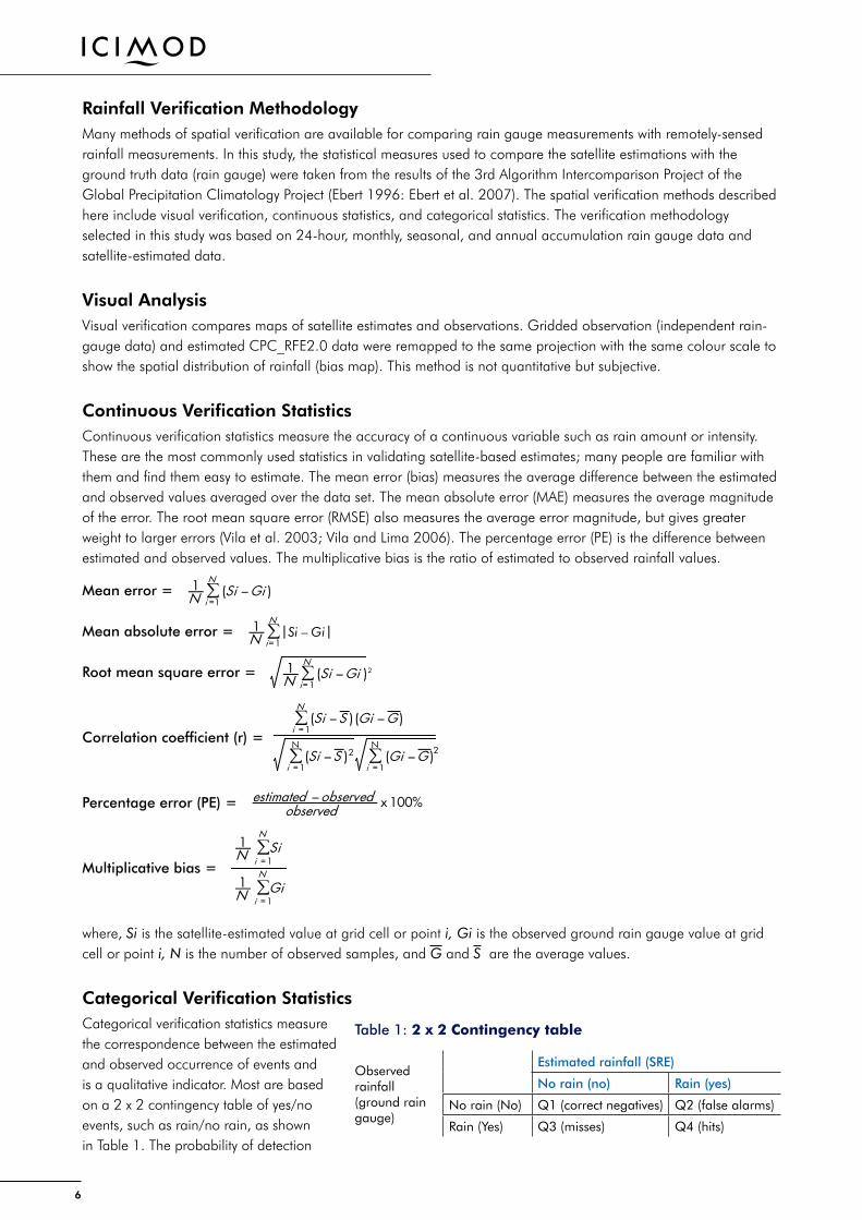
Categorical Verification StatisticsCategorical verification statistics measure the correspondence between the estimated and observed occurrence of events and is a qualitative indicator. Most are based on a 2 x 2 contingency table of yes/no events, such as rain/no rain, as shown in Table 1. The probability of detection

Table 1: 2 x 2 Contingency table

Observed rainfall(ground rain gauge)

Estimated rainfall (SRE)

No rain (no) Rain (yes)

No rain (No) Q1 (correct negatives) Q2 (false alarms)

Rain (Yes) Q3 (misses) Q4 (hits)

7

(POD) measures the fraction of observed events that was diagnosed correctly and is sometimes called the ‘hit rate’. The false alarm ratio (FAR) gives the fraction of diagnosed events that were actually non-events (Ebert et al. 2007). The POD and FAR should always be used together. These and other measures are described in more detail below (based on information from www.cawcr.gov.au/projects/verification/).

Rain/no rain contingency table: The off-diagonal elements in the table characterize the error. The elements in the table (hits, misses, false alarms, correct negatives) give the joint distribution of events, while the elements above and to the right (observed yes, observed no, others) are called the marginal distributions. In the table, correct negatives (Q1) represent correctly estimated no rain events, false alarms (Q2) represent when rain was estimated by satellite but did not occur on the ground, misses (Q3) represent when rain was not estimated by satellite but did occur on the ground, and hits (Q4) represent correctly estimated rain events, where both satellite estimates and rain gauges show rain. The contingency table is a useful way to see what types of errors are being made. A perfect estimate system would produce only hits and correct negatives and no misses or false alarms. Basic statistics are used to provide information on rain identification through contingency tables taken together with conditional rain rates (0 or 1 mm/day rain/no rain thresholds). This type of table was used to measure the skill of the rainfall estimations in pinpointing rain where rain was observed on the ground.

Probability of detection (POD) = Q3 +Q4Q4 or = hits + misses

hits

The POD is sensitive to hits, but ignores false alarms. It is very sensitive to the climatology of the region and is good for rare events. It can be artificially improved by issuing more ‘yes’ estimates to increase the number of hits. It should be used in conjunction with the false alarm ratio. POD is also an important component of the relative operating characteristic (ROC) used widely for probability estimates. It ranges from 0 to 1; the perfect score is 1.

False alarm ratio (FAR) = Q2 +Q4Q2 or = hits + false alarms

false alarms

The FAR is sensitive to false alarms, but ignores misses. It is very sensitive to the climatological frequency of the event and should be used in conjunction with the probability of detection. It ranges from 0 to 1; the perfect score is 0.

In Phase 1, the study focused only on POD and FAR. These categorical statistics are affected by the climatology of the study region and might not be useful for comparing rain detection accuracy over two different climatic regions, for example the higher Himalayan and Siwalik regions. Therefore in Phase 2, a rigorous and optimum analysis was carried out to obtain significant results and some additional measurements were added to the categorical verification statistics such as the threat score (TS) and equitable threat score (ETS). These are not affected as much by wetness or dryness of the regions, thus this type of comparison is good for regional or general climatology.

Threat score (TS) = hits + misses + false alarmshits

The TS measures the fraction of observed and/or estimated events that were correctly estimated. It can be thought of as the accuracy after correct negatives have been removed, in other words TS is only concerned with estimates that count. TS is sensitive to hits and penalizes both misses and false alarms. It does not distinguish the source of estimated error. TS does depend on the climatological frequency of events, with poorer scores for rarer events since some hits can occur due to random chance. It ranges from 0 to 1; the perfect score is 1; 0 indicates no skill.

Equitable threat score (ETS) = hits + misses + false alarms – hits

hits – hitsrandomrandom

where

random = Total(hitshits

+misses) (hits + fale alarms)

The ETS measures the fraction of observed and/or estimated events that were correctly predicted, adjusted for hits associated with random chance (for example, it is easier to correctly estimate rain occurrence in a wet climate than in a dry climate). The ETS is often used in the verification of rainfall in numerical weather prediction models because its ‘equitability’ allows scores to be compared more fairly across different regimes. It is sensitive to hits. It penalizes both misses and false alarms in the same way and thus does not distinguish the source of estimated error. It ranges from -1/3 to 1; the perfect score is 1, 0 indicates no skill.

8

Analysis and Results

The SRE were evaluated at various temporal scales: daily, monthly, seasonal, and annual. The results of the comparison of satellite-estimated and gauge-observed data are summarized below.

Comparison of Quantitiative Rainfall Distribution

Daily rainfall distribution as estimated from CPC_RFE2.0A comparison was made of the rainfall distribution in the six years from 2002 to 2007. In the visual analysis, two kinds of comparison were made:

Grid-to-grid comparison – in this method, all the grids lying within the country boundary are considered

Point-to-point comparison – in this method, only those grids which have at least one rain-gauge (point data) are considered. The location of grids with one or more stations is shown in Figure 4. The grids are categorized according to the station elevation.

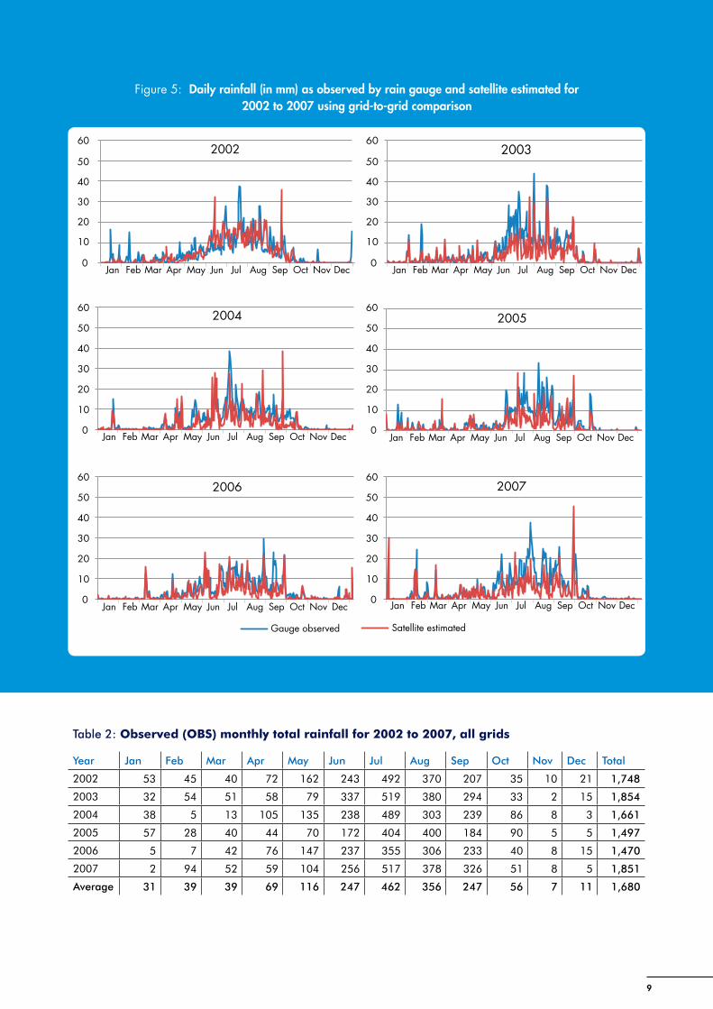
Figure 5 shows the time series of satellite-estimated (CPC_RFE2.0) and observed (rain gauge) daily rainfall for each year from 2002 to 2007 using grid-to-grid comparison. Qualitatively, the rainfall events generally match. Quantitatively, the CPC_RFE2.0 tends to substantially underestimate, but there are also some events where the CPC_RFE2.0 is greater than the observed value. The CPC_RFE2.0 overestimates are mostly during cooler months and when rainfall is low or moderate. In the rainy season, the difference between the two is more evident.

Figure 6 shows the same comparison using the point-to-point method. The underestimation by SRE is more evident, although there is little quantitative difference between the graphs prepared by the two methods.

Monthly rainfall distribution as estimated from CPC_RFE2.0The monthly accumulated gauge-observed and satellite-estimated rainfall totals for the whole country (all grids) for each year from 2002 to 2007 are given in Tables 2 and 3 and shown in graph format in Figure 7 (grid-to-grid comparison). The data using only those grids that have a gauge station is given in Tables 4 and 5 and shown in graph format in Figure 8 (point-to-point comparison).

The differences between the observed and satellite-estimated data become clearer when the data is presented in monthly form. During the low rainfall months from October to April, the CPC_RFE2.0 estimation exhibits good results close to those of the observed data. In the higher rainfall months from May to September, it tends to underestimate, with significant underestimation in the main monsoon months which have more than 70 per cent of the annual total rainfall. The grid-to-grid comparison shows a total average annual rainfall deficiency for 2002 to 2007 of 627 mm, of which 548 mm occurs during the monsoon season. The point-to-point comparison shows slightly higher total rainfall values, both for observed rainfall (1,798 mm compared to 1,680 mm) and for the satellite estimates (1,104 mm compared to 1,054 mm). The annual rainfall deficiency using the satellite estimates is also slightly, but not significantly, higher: 695 mm, of which 587 mm occurs during the monsoon season. As the differences were not significant, only grid-to-grid comparisons were used for spatial maps and further analysis.

Figure 4: Location of grids with one or more gauge station

9

Figure 5: Daily rainfall (in mm) as observed by rain gauge and satellite estimated for 2002 to 2007 using grid-to-grid comparison

Table 2: Observed (OBS) monthly total rainfall for 2002 to 2007, all grids

Year Jan Feb Mar Apr May Jun Jul Aug Sep Oct Nov Dec Total

2002 53 45 40 72 162 243 492 370 207 35 10 21 1,748

2003 32 54 51 58 79 337 519 380 294 33 2 15 1,854

2004 38 5 13 105 135 238 489 303 239 86 8 3 1,661

2005 57 28 40 44 70 172 404 400 184 90 5 5 1,497

2006 5 7 42 76 147 237 355 306 233 40 8 15 1,470

2007 2 94 52 59 104 256 517 378 326 51 8 5 1,851

Average 31 39 39 69 116 247 462 356 247 56 7 11 1,680

Gauge observed Satellite estimated

0

10

20

30

40

50

602002

Jan Feb Mar Apr May Jun Jul Aug Sep Oct Nov Dec0

10

20

30

40

50

602003

Jan Feb Mar Apr May Jun Jul Aug Sep Oct Nov Dec

0

10

20

30

40

50

602005


0

10

20

30

40

50

602007


0

10

20

30

40

50

602004


0

10

20

30

40

50

602006


10

Figure 6: Daily rainfall (in mm) as observed by rain gauge and satellite estimated for 2002 to 2007 using point-to-point comparison

Table 3: Satellite-estimated (SRE) monthly total rainfall for 2002 to 2007, all grids


2002 53 52 52 71 73 181 186 239 119 81 13 20 1,141

2003 33 43 58 55 57 165 290 245 209 39 3 11 1,209

2004 34 4 5 82 62 191 267 216 143 45 1 3 1,056

2005 35 28 48 34 43 90 231 174 142 43 2 2 871

2006 6 3 36 43 100 177 247 183 122 25 7 37 986

2007 49 52 43 58 69 103 292 168 208 15 2 2 1,062

Average 35 30 41 57 67 151 252 204 157 41 5 13 1,054

0

10

20

30

40

50

602002

0

10

20

30

40

50

602003

0

10

20

30

40

50

602004

0

10

20

30

40

50

602005

0

10

20

30

40

50

602006

0

10

20

30

40

50

602007

Gauge observed Satellite estimated

Jan Feb Mar Apr May Jun Jul Aug Sep Oct Nov Dec Jan Feb Mar Apr May Jun Jul Aug Sep Oct Nov Dec



11

Table 4: Observed (OBS) monthly total rainfall for 2002 to 2007, grids with stations


2002 46 30 30 70 186 281 572 385 215 32 7 20 1,874

2003 29 46 47 61 83 385 578 400 315 34 0 16 1,992

2004 32 0 4 106 151 273 561 316 276 78 4 0 1,801

2005 46 12 37 46 77 191 417 440 179 107 0 2 1,553

2006 0 0 33 84 172 259 368 328 268 43 0 13 1,569

2007 0 95 38 64 111 298 576 399 376 42 4 0 2,002

Average 26 30 32 72 130 281 512 378 272 56 3 8 1,798

Figure 7: Monthly total rainfall (in mm) as observed by rain gauge and satellite estimated for 2002 to 2007 using grid-to-grid comparison

0

100

200

300

400

500

600


2002

0

100

200

300

400

500

600


2003

0

100

200

300

400

500

600


2004

0

100

200

300

400

500

600


2005

0

100

200

300

400

500

600


2006

0

100

200

300

400

500

600


2007

Satellite estimatedGauge observed

12

Table 5: Satellite-estimated (SRE) monthly total rainfall for 2002 to2007, grids with stations


2002 46 31 34 65 64 211 241 246 118 54 6 17 1,133

2003 20 23 49 48 46 189 336 269 215 39 0 7 1,242

2004 28 0 3 82 70 211 297 249 145 41 0 1 1,126

2005 22 14 41 33 38 110 248 203 147 44 0 0 899

2006 0 1 28 43 112 205 264 199 144 25 2 38 1,061

2007 54 47 28 63 67 122 322 187 257 13 0 0 1,162

Average 28 19 30 56 66 175 285 226 171 36 1 11 1,104

Figure 8: Monthly total rainfall (in mm) as observed by rain gauge and satellite estimated for 2002 to 2007 using point-to-point comparison

0

100

200

300

400

500

600


2002

0

100

200

300

400

500

600


2003

0

100

200

300

400

500

600


2004

0

100

200

300

400

500

600


2005

0

100

200

300

400

500

600


2006

0

100

200

300

400

500

600


2007


13

Seasonal distribution of rainfall as estimated from CPC_RFE2.0The values of the gauge-observed (OBS) and satellite-estimated (SRE) seasonal rainfall totals for each year from 2002 to 2007 (all grids) are given in Table 6, together with the seasonal means for the whole period. Figure 9 shows the seasonal totals in graph format. Most of the rain falls during the monsoon season (June to September) which had 78 per cent of the observed and 72 per cent of the satellite-estimated rainfall over the whole period. In the winter season (December-January-February), the satellite estimates are close to the observed values; in the pre-monsoon (March-April-May) and post-monsoon (October-November) seasons, the satellite estimates are generally somewhat lower than the observed values; and in the monsoon (June-July-August-September) season, the satellite estimates are far lower than the observed values, on average by 548 mm.

Comparison of Spatial Distribution of Rainfall as Estimated from CPC_RFE2.0 and Gauge-Observed DataEven when one-dimensional statistics for two data sets are very similar, the spatial continuity may be quite different. The statistical analysis provides information on descriptive statistics such as the mean, mode, correlation, and mean error. Spatial analysis provides additional information on the spatial variation. The spatial distribution of rainfall is very important for applications in meteorology, hydrology, and other environmental sciences. One of the main objectives of using the CPC_RFE2.0 estimated rainfall data is to apply it in flood forecasting and warning using a hydrological flood forecasting model; thus spatial consistency with the observed rainfall is very important.

Analyses of spatial distribution were performed on a daily basis and then accumulated to show the annual, seasonal, and monthly spatial distribution of rainfall. The spatial distribution of the annual (January 1 to December 31), monsoon, and winter season observed (gauge-observed) and CPC_RFE2.0 (satellite-estimated) rainfall means for each grid for each of the years from 2002 to 2007 are presented in Figures 10, 11, and 12.

The maps show a marked variation in both amount and spatial pattern between the estimated CPC_RFE2.0 rainfall and the observed annual values. The observed values show a generally decreasing trend in rainfall from east to west with numerous pockets of high rainfall. The CPC_RFE2.0 estimated values show a decreasing trend from south to north. The lowest observed rainfall is in an area around 83º45’E and 29ºN, which is a trans-Himalayan rain shadow region north of the Annapurna Himalayan range. The observed values show a high rainfall area around Lumle (83°48’17”E and 28°17’53”N) in central Nepal which is not captured by the CPC_RFE2.0 at all, as was observed in a comparison with the GSMaP satellite product (Shrestha et al. 2011). The CPC_RFE2.0 actually indicates that the maximum rainfall is in the central south and far southwestern areas.

Around 70 per cent of the annual rainfall is in the monsoon season, thus the maps for this season are very similar to those for annual rainfall, except that the total amounts are slightly less (Figure 11).

The winter season maps (December, January, and February) are very different (Figure 12). In contrast to the annual and monsoon values, in many places, the CPC_RFE2.0 estimates are higher than the observed values, especially

Table 6: Seasonal distribution of rainfall as observed by rain gauge (OBS) and satellite estimated (SRE) for 2002 to 2007 (all grids)

OBS SRE

Season Season

Year DJF MAM JJAS ON DJF MAM JJAS ON

2002 108 274 1,311 45 118 197 725 94

2003 107 188 1,530 35 95 171 909 42

2004 58 252 1,269 94 49 149 818 47

2005 88 154 1,159 95 66 125 638 44

2006 17 265 1,130 48 11 179 729 32

2007 111 214 1,477 59 138 170 771 17

Mean 82 224 1,313 62 80 165 765 46

14

Figure 9: Seasonal rainfall (in mm) as observed by rain gauge and satellite estimated for 2002 to 2007 (all grids)

in the western part of Nepal. This means that the bias is less in this season and suggests that the application of bias correction for flood forecasting should be made with caution.

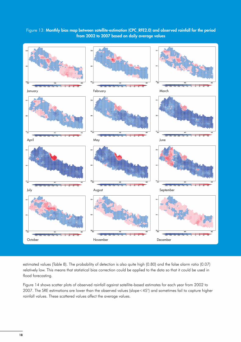
Monthly Bias Map Preparation and AnalysisA bias map provides information on whether the model predictions (in this case, the satellite-based estimates) are overestimated or underestimated. Bias maps were prepared for each month using the average daily observed and satellite-estimated rainfall values over all years from 2002 to 2007 (Figure 13). Red shading in the bias map indicates areas where the satellite-estimated values are higher than the observed rainfall values (positive bias); blue shading indicates areas where the satellite-estimated values are lower than the observed rainfall values (negative bias). The intensity of the colour reflects the extent of the over or underestimation. The values of the monthly total

0

400

800

1200

1600

DJF MAM JJAS ON

2002

0

400

800

1200

1600

DJF MAM JJAS ON

2003

0

400

800

1200

1600

DJF MAM JJAS ON

2004

0

400

800

1200

1600

DJF MAM JJAS ON

2005

0

400

800

1200

1600

DJF MAM JJAS ON

2006

0

400

800

1200

1600

DJF MAM JJAS ON

2007


15

bias over the whole country for each year for 2002 to 2007 and the mean values for the whole period are given in Table 7.

Over all years, satellite estimation shows an average annual negative bias of 627 mm (Table 7). The satellite-estimated values show both positive and negative values at different places in all months, but with a negative bias on average in most months (Figure 13, Table 7). Overall, the negative bias is least in November and highest in July, and there is a small positive bias in December, January, and March. Throughout the year, there is marked positive bias over the rain shadow region in the Annapurna Himalayan range.

Figure 10: Spatial distribution of annual total rainfall (in mm) as observed by rain gauge (OBS) and satellite estimated (SRE) for 2002 to 2007 (all grids)

Annual total rainfall 2002 (SRE)






Annual total rainfall 2002 (OBS)






16

Table 7: Monthly, six-year monthly mean, and annual total values of total bias (all grids) of satellite-estimated (CPC_RFE2.0) compared to observed rainfall values for 2002 to 2007Year Jan Feb Mar Apr May Jun Jul Aug Sep Oct Nov Dec Total

2002 1 8 12 -1 -88 -61 -306 -131 -88 46 3 -2 -607

2003 0 -11 8 -3 -22 -172 -229 -136 -85 6 1 -5 -646

2004 -4 -1 -7 -23 -73 -47 -222 -87 -96 -40 -7 0 -605

2005 -22 0 8 -11 -27 -81 -172 -227 -41 -47 -3 -3 -626

2006 1 -5 -6 -34 -47 -60 -108 -123 -111 -15 -1 22 -485

2007 47 -42 -9 -1 -35 -152 -224 -211 -118 -37 -6 -3 -791

Average 4 -8 1 -12 -49 -95 -210 -152 -90 -15 -2 2 -627

Figure 11: Spatial distribution of total monsoon rainfall (in mm) as observed by rain gauge (OBS) and satellite estimated (SRE) for 2002 to 2007 (all grids)

Monsoon season total rainfall 2002 (SRE)


Monsoon season total rainfall 2002 (OBS)










17

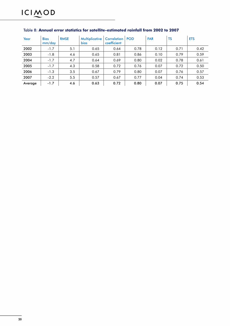
Error Statistics for Satellite-Based Rainfall EstimateThe overall error statistics for the satellite-estimated rainfall for the period from 2002 to 2007 derived from the daily satellite-estimated values are summarized in Table 8. The table shows the values for bias rainfall, root mean square error (RMSE), multiplicative bias, correlation coefficient, probability of detection (POD), false alarm ratio (FAR), threat score (TS), and equitable threat score (ETS). A contingency table was also derived through categorical analysis using a rainfall threshold value of 1 mm. Changing the threshold value might result in slight changes in the table.

The average daily rainfall bias is -1.72 mm. Accumulation of the bias over a year leads to an underestimation of more than 600 mm – a significant amount. Equally, there is a 72 per cent correlation between the observed and

Figure 12: Spatial distribution of total winter season rainfall (in mm) as observed by rain gauge (OBS) and satellite estimated (SRE) for 2002 to 2007 (all grids)

Winter season total rainfall 2002 (SRE)

Winter season total rainfall 2002 (OBS)











18

estimated values (Table 8). The probability of detection is also quite high (0.80) and the false alarm ratio (0.07) relatively low. This means that statistical bias correction could be applied to the data so that it could be used in flood forecasting.

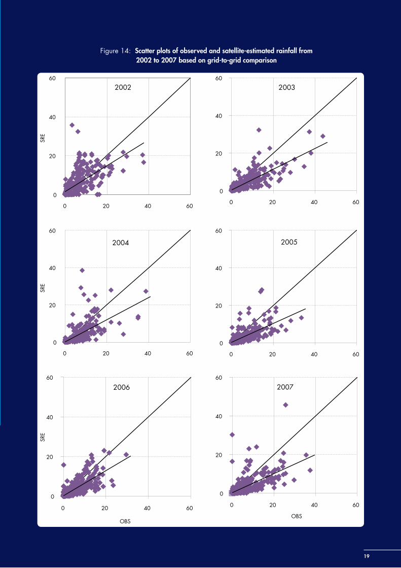
Figure 14 shows scatter plots of observed rainfall against satellite-based estimates for each year from 2002 to 2007. The SRE estimations are lower than the observed values (slope<45°) and sometimes fail to capture higher rainfall values. These scattered values affect the average values.

Figure 13: Monthly bias map between satellite-estimation (CPC_RFE2.0) and observed rainfall for the period from 2002 to 2007 based on daily average values

January

April

July

October

February

May

August

November

March

June

September

December

19

Figure 14: Scatter plots of observed and satellite-estimated rainfall from 2002 to 2007 based on grid-to-grid comparison

0

20

40

60

0 20 40 60

SRE

2002

0

20

40

60

0 20 40 60

2003

0

20

40

60

0 20 40 60

SRE

2004

0

20

40

60

0 20 40 60

2005

0

20

40

60

0 20 40 60

SRE

OBS

2006

0

20

40

60

0 20 40 60

OBS

2007

20

Table 8: Annual error statistics for satellite-estimated rainfall from 2002 to 2007

Year Bias mm/day

RMSE Multiplicative bias

Correlation coefficient

POD FAR TS ETS

2002 -1.7 5.1 0.65 0.64 0.78 0.12 0.71 0.42

2003 -1.8 4.6 0.65 0.81 0.86 0.10 0.79 0.59

2004 -1.7 4.7 0.64 0.69 0.80 0.02 0.78 0.61

2005 -1.7 4.3 0.58 0.72 0.76 0.07 0.72 0.50

2006 -1.3 3.5 0.67 0.79 0.80 0.07 0.76 0.57

2007 -2.2 5.5 0.57 0.67 0.77 0.04 0.74 0.53

Average -1.7 4.6 0.63 0.72 0.80 0.07 0.75 0.54

21

Discussion and Conclusion

Satellite-Estimated Values The different comparisons of satellite-estimated and observed rainfall all show that the CPC_RFE2.0 underestimates strongly on an annual basis, with a calculated average annual deficit of 627 mm over the whole country. In the high rainfall area in and around Lumle, the difference exceeds 2,000 mm. As expected, this pattern is the same in the monsoon season. However, during the winter season there are more areas where the estimated rainfall is higher than observed. Overall, the lowest bias is found during the winter season, with the minimum negative bias in November, and a small positive bias in December, January, and March. As the monsoon approaches, the bias increases, reaching a maximum in July. There is no definite pattern in the bias map.

The daily bias rainfall was -1.72 mm, with a correlation coefficient of 0.72, root mean square error of 4.62 mm, and multiplicative bias of 0.63 when all the grids in the country were considered. When considering only those grids with stations, the bias was -1.90 mm, correlation coefficient 0.73, root mean square error 5.23 mm, and multiplicative bias 0.61. Thus there was little difference in bias regardless of whether all grids were used or only those that contained a station.

Improving ValuesSince the annual bias is very high, the rainfall estimates need to be improved before they can be used in a model. There are two main ways to improve the estimation: applying a bias correction and improving the SRE algorithm.

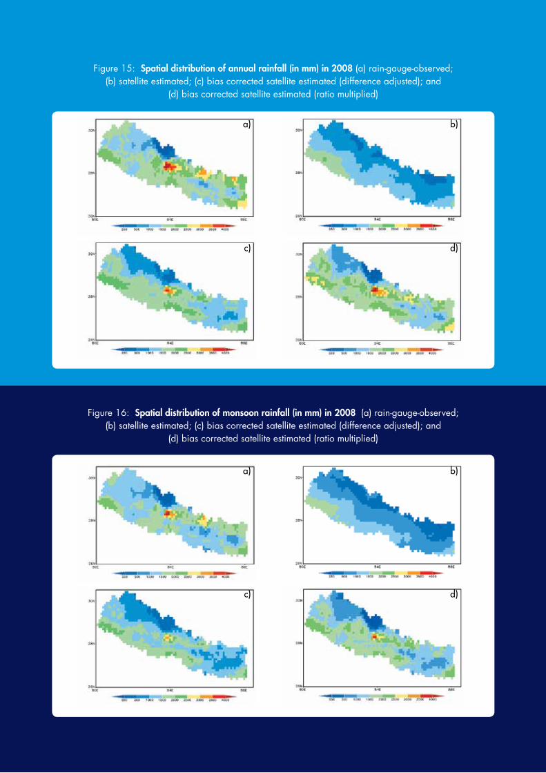
Bias correctionThe correlation and probability of detection values between the satellite-estimated and observed data were quite high, and the false alarm ratio was relatively low, thus in principle it is possible to apply a bias correction based on statistical analysis. Two methods were used to investigate the results of applying a bias correction. Bias corrections were calculated from the daily average rainfall from 2002 to 2007 and applied to the values for 2008. In the first method, the mean difference between the observed and estimated values was calculated for each grid and adjusted. In the second method, a ratio or multiplication factor was calculated for each grid and a correction was applied to those grids in which the rainfall amount was greater than a threshold value of 1.0 mm.

Figure 15 shows the observed (averaged), satellite-estimated, and two different bias corrected satellite-estimated values of annual total rainfall for 2008. Figures 16 and 17 show the maps for the monsoon and winter seasons separately. The annual and monsoon rainfall maps were significantly improved after the bias adjustments and show a much greater similarity to the map of observed values, with the greatest improvement using the ratio multiplied method. The amount of rainfall in the winter season is quite low and there was little difference between the estimated and observed values or the values following bias correction. Bias correction may not be needed in this season.

The accumulated monthly rainfall values for 2008 – observed, satellite-estimated, and after bias correction – are summarized in Table 9 and shown graphically in Figure 18. The rainfall values were significantly improved after bias adjustment, especially using the ratio multiplied method, but there is still a considerable discrepancy in the monsoon months, indicating the need for further research and study. One possibility that could be considered is that of developing a variable bias correction based on estimated rainfall amount.

Improving the algorithmThe algorithm used to derive the SRE data has not yet been fully optimized for use in the Himalayan region with its extreme variations in topography and rainfall. For example, at present the basic algorithm ignores GTS data when more than 200 mm is reported. But in the HKH region, there are many rainfall events in a year with more than 200 mm per day, and this restriction should be reviewed. Orographic effects are also not considered in the present SRE. The cloud top temperature in the algorithm could be reconsidered, as orography is always present in

22

Figure 15: Spatial distribution of annual rainfall (in mm) in 2008 (a) rain-gauge-observed; (b) satellite estimated; (c) bias corrected satellite estimated (difference adjusted); and

(d) bias corrected satellite estimated (ratio multiplied)

Figure 16: Spatial distribution of monsoon rainfall (in mm) in 2008 (a) rain-gauge-observed; (b) satellite estimated; (c) bias corrected satellite estimated (difference adjusted); and


a)

c)

b)

d)

a)

c)

b)

d)

050

100150200250300350400450500

Jan

Feb

Mar

Apr

May Ju

n Jul

Aug Sep

Oct

Nov Dec

ObservedSatellite-estimatedBias corrected satellite-estimated (differenceadjusted)Bias corrected satellite-estimated (ratio multiplied)

Figure 18: Monthly total rainfall (in mm) for 2008

23

rainfall whether it is from the monsoon or western disturbances. Cloud top temperatures in orographic rain are greater than the threshold values in the present algorithm. The Nepalese Himalayas are always covered by snow, and it seems likely that the sensor is taking this as a cloud top temperature, especially during the winter season, and hence detecting rainfall. This may be one reason for the CPC_RFE2.0 values showing a decreasing trend from south to north and being higher than the observed values in rain shadow areas and during the winter period.

Figure 17: Spatial distribution of winter rainfall (in mm) in 2008 (a) rain-gauge-observed; (b) satellite estimated; (c) bias corrected satellite estimated (difference adjusted); and


Table 9: Monthly total observed and estimated rainfall in 2008 (mm)

Jan Feb Mar Apr May Jun Jul Aug Sep Oct Nov Dec Total

Rain-gauge-observed 10 4 17 48 116 372 427 429 210 31 1 0 1,664

CPC_RFE2.0 estimated 5 3 1 35 55 222 204 246 183 12 0 1 968

CPC_RFE2.0 estimated, bias corrected (difference adjusted) 7 4 1 38 86 312 368 387 218 17 0 0 1,438

CPC_RFE2.0 estimated, bias corrected (ratio multiplied) 13 3 4 33 112 400 376 423 215 35 0 1 1,616

a)

c)

b)

d)

24

Conclusion Nepal is a mountainous country, and it is extremely difficult to install and maintain rain gauges in remote areas where access is difficult. SRE can provide rainfall estimates for each pixel over a domain and thus has tremendous potential to provide data to support monitoring of flood and drought.

This assessment of the accuracy of the CPC_RFE2.0 indicates that the data need to be improved before they can be used in modelling. Ideally, the algorithm itself should be improved before being implemented. Now that one decade of SRE values are available, it may be possible to use the SRE climatology to improve the SRE algorithm. However, this tends to be a time-consuming process, and improvements in one area may disrupt other parts of the domain. Until a revised improved version of the CPC_RFE2.0 becomes available, we recommend that SRE bias correction (spatial and temporal) is applied before the results are used in further applications.

25

References

Adler, RF; Chang, GJ; Ferraro, R; Xie, P; Janowiak, J; Rudolf, B; Schneider, U; Curtis, S; Bolvin, D; Gruber, A; Susskind, J; Arkin, P; Nelkin, E ( 2003) ‘The version-2 Global Precipitation Climatology Project (GPCP) monthly precipitation analysis (1979-present).’ J. Hydrometeorol. 4: 1147–1167

Artan, GA; Gadain, H; Smith, JL; Asante, K; Bandaragoda, CJ; Verdin, JP (2007) ‘Adequacy of satellite derived rainfall data for streamflow modelling.’ Nat. Hazards 43: 167-185

Basistha, A; Arya, DS; Goel. NK (2007) ‘Spatial distribution of rainfall in Indian Himalayas – A case study of Uttarakhand region.’ Water Resources Management 22: 1325–1346. DOI 10.1007/s11269-007-9228-2

Clark, I (2001) Practical geostatics. Alloa, Scotland, UK: Geostokos Limited. www.kriging.com/PG1979/PG1979.pdf (accessed 26 February 2013)

Dinku, T; Chidzambwa, S; Ceccato, P; Connor, SJ; Ropelewski, CF (2008) ‘Validation of high-resolution satellite rainfall products over complex terrain.’ Int. J. Remote Sens. 29(14): 4097–4110

Ebert, EE (1996) Result of the 3rd Algorithm Intercomparison Project (AIP-3) of the Global Precipitation Climatology Project (GPCP), Bureau of Meteorology Centre, Report No 55. Melbourne, Australia: Bureau of Meteorology Centre

Ebert, EE; Janowiak, JE; Kidd, C (2007) ‘Comparison of near-real-time precipitation estimates from satellite observations and numerical models’. Bull. Amer. Meteorol. Soc. 88(1): 47–64

Hong, Y; Adler, RF; Negri, A; Huffman, GJ (2007) ‘Flood and landslide applications of near real-time satellite rainfall estimation.’ Nat. Hazards 43: 285–294

Huffman, GJ; Adler, RF; Bolven, DT; Gu, G; Nelkin, EJ; Bowman, KP; Hong, Y; Stocker, EF; Wolfe, DB (2007) ‘The TRMM Multisatellite Precipitation Analysis (TMPA): Quasi-global, multiyear, combined-sensor precipitation estimates at fine scales.’ J. Hydrometeorol. 8: 38–55

Isaaks, EH; Srivastava, RM (1989) Applied geostatics. Oxford, UK: Oxford University Press

Joyce, JJ; Janowiak, JE; Arkin, PA; Xie, P (2004) ‘CMORPH: A method that produces global precipitation estimates from passive microwave and infrared data at high spatial and temporal resolution.’ J. Hydrometeorol. 5: 487–503

Khanal, N; Shrestha, M; Ghimire, M (2007) Preparing for flood disaster: Mapping and assessing hazard in the Ratu watershed. Kathmandu, Nepal: ICIMOD

Kidd, C (2005) ‘Validation of satellite rainfall estimates over the mid-latitudes.’ In Proceedings of the 2nd IPWG working group workshop, Monterey, CA, 25-28 October 2004, pp 205-215. Monterey CA, USA: Naval Research Laboratory, Marine Meteorology Division, and Darmstadt, Germany: EUMETSAT

Kubota, T; Ushio, T; Shige, S; Kachi, M; Okamoto, K (2009) ‘Verification of high resolution satellite-based rainfall estimates around Japan using a gauge-calibrated ground-radar dataset.’ J. Meteorol. Soc. Japan 87A: 203–222

Laurent, H; Jobard, I; Toma, A (1998) ‘Validation of satellite and ground based estimates of precipitation over the Sahel.’ Atmospheric Research 47-48: 651-670

Shrestha, MS; Artan, GA; Bajracharya, SR; Sharma, RR (2008a) ‘Applying satellite-based rainfall estimates for streamflow modelling in the Bagmati Basin, Nepal.’ J. Flood Risk Management 1: 89–99

Shrestha, MS; Bajracharya, SR; Mool, P (2008b) Satellite rainfall estimation in the Hindu Kush-Himalayan Region. Kathmandu, Nepal: ICIMOD

Shrestha, MS; Takara, K; Kubota, T; Bajracharya, SR (2011) ‘Verification of GSMaP rainfall estimates over the central Himalayas.’ Annual Journal of Hydraulics Engineering, JSCE 55: 38-42

UNDP (2004) Reducing disaster risk: A challenge for development. New York: Bureau for Crisis Prevention and Recovery – United Nations Development Programme (BCPR-UNDP) www.preventionweb.net/english/professional/publications/v.php?id=1096 (accessed 26 February 2013

Ushio, T; Sasashige, K; Kubota, T; Shige, S; Okamota, K; Aonashi, K; Inoue, N; Takahashi, T; Iguchi, T; Kachi, M; Oki, R; Morimoto, T; Kawasaki, ZI (2009) ‘A Kalman filter approach to the global satellite mapping of precipitation (GS_Map) from combined passive microwave and infrared radiometric data.’ J. Meteorol. Soc. Japan 87A: 137–151

Vila, D; Scofield, R; Kuligowski, R; Davenport, J (2003) Satellite rainfall estimation over South America: Evaluation of two major events, NOAA Technical Report NESDIS 114. Washington DC, USA: U.S. Department of Commerce, National Oceanic and Atmospheric Administration

Vila, D; Lima, A (2006) ‘Satellite rainfall estimation over South America: The hydroestimator technique.’ In WW Grabowski (ed) 14th International Conference on Clouds and Precipitation, Bologna, Italy, 18–23 July 2004. Amsterdam, Netherlands: Elsevier

26

Source: District Agriculture Development Office- Mustang, 2010

Xie, P; Arkin, PA (1996) ‘Analyses of global monthly precipitation using gauge observations, satellite estimates and numerical model predictions’. J. Clim. 9: 840–858

Xie, P; Yarosh, Y; Love, T; Janowiak, J; Arkin, PA (2002) ‘A real-time daily precipitation analysis over South Asia.’ Preprints of the 16th Conference on Hydrology, Orlando, Florida. Washington DC, USA: American Meteorological Society

27

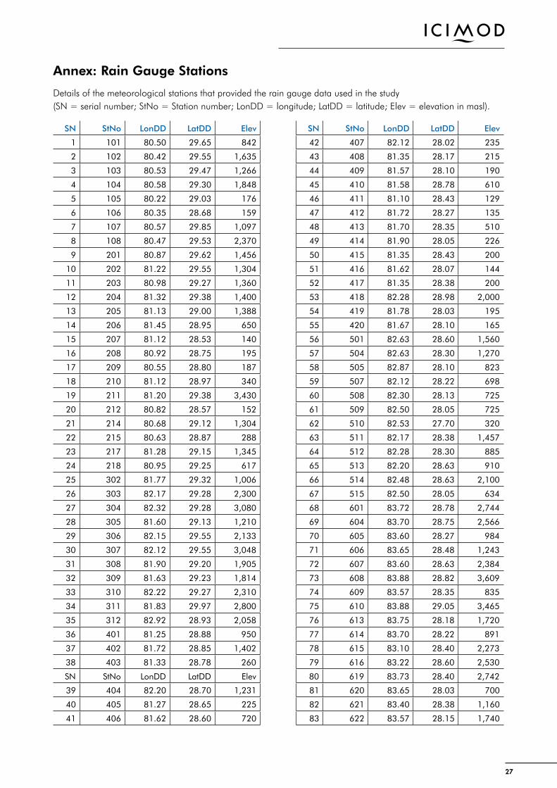
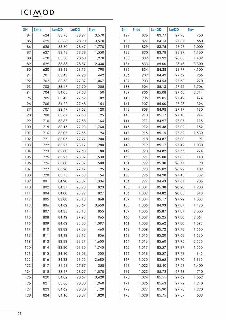
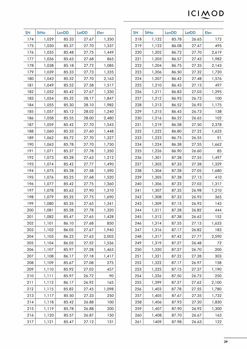
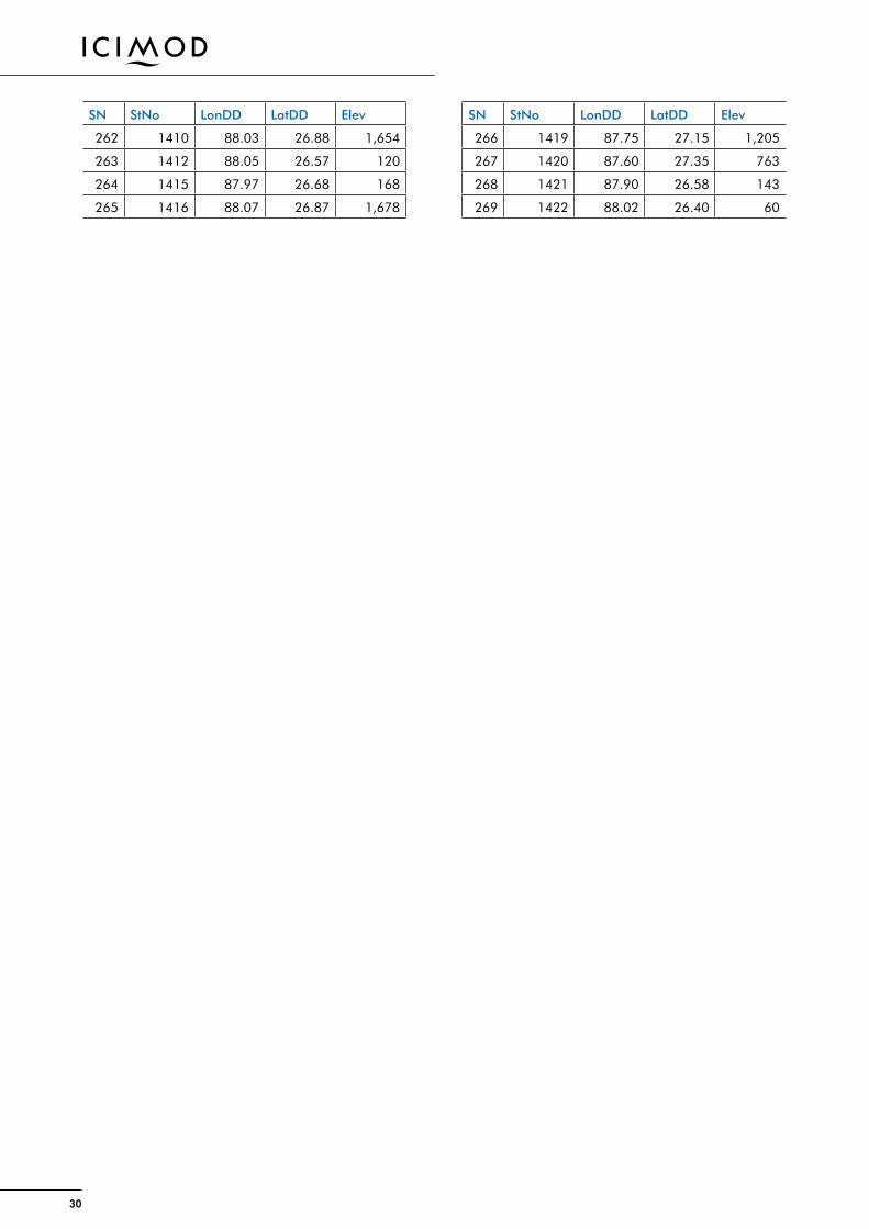
Annex: Rain Gauge Stations

Details of the meteorological stations that provided the rain gauge data used in the study (SN = serial number; StNo = Station number; LonDD = longitude; LatDD = latitude; Elev = elevation in masl).

SN StNo LonDD LatDD Elev SN StNo LonDD LatDD Elev

1 101 80.50 29.65 842 42 407 82.12 28.02 235

2 102 80.42 29.55 1,635 43 408 81.35 28.17 215

3 103 80.53 29.47 1,266 44 409 81.57 28.10 190

4 104 80.58 29.30 1,848 45 410 81.58 28.78 610

5 105 80.22 29.03 176 46 411 81.10 28.43 129

6 106 80.35 28.68 159 47 412 81.72 28.27 135

7 107 80.57 29.85 1,097 48 413 81.70 28.35 510

8 108 80.47 29.53 2,370 49 414 81.90 28.05 226

9 201 80.87 29.62 1,456 50 415 81.35 28.43 200

10 202 81.22 29.55 1,304 51 416 81.62 28.07 144

11 203 80.98 29.27 1,360 52 417 81.35 28.38 200

12 204 81.32 29.38 1,400 53 418 82.28 28.98 2,000

13 205 81.13 29.00 1,388 54 419 81.78 28.03 195

14 206 81.45 28.95 650 55 420 81.67 28.10 165

15 207 81.12 28.53 140 56 501 82.63 28.60 1,560

16 208 80.92 28.75 195 57 504 82.63 28.30 1,270

17 209 80.55 28.80 187 58 505 82.87 28.10 823

18 210 81.12 28.97 340 59 507 82.12 28.22 698

19 211 81.20 29.38 3,430 60 508 82.30 28.13 725

20 212 80.82 28.57 152 61 509 82.50 28.05 725

21 214 80.68 29.12 1,304 62 510 82.53 27.70 320

22 215 80.63 28.87 288 63 511 82.17 28.38 1,457

23 217 81.28 29.15 1,345 64 512 82.28 28.30 885

24 218 80.95 29.25 617 65 513 82.20 28.63 910

25 302 81.77 29.32 1,006 66 514 82.48 28.63 2,100

26 303 82.17 29.28 2,300 67 515 82.50 28.05 634

27 304 82.32 29.28 3,080 68 601 83.72 28.78 2,744

28 305 81.60 29.13 1,210 69 604 83.70 28.75 2,566

29 306 82.15 29.55 2,133 70 605 83.60 28.27 984

30 307 82.12 29.55 3,048 71 606 83.65 28.48 1,243

31 308 81.90 29.20 1,905 72 607 83.60 28.63 2,384

32 309 81.63 29.23 1,814 73 608 83.88 28.82 3,609

33 310 82.22 29.27 2,310 74 609 83.57 28.35 835

34 311 81.83 29.97 2,800 75 610 83.88 29.05 3,465

35 312 82.92 28.93 2,058 76 613 83.75 28.18 1,720

36 401 81.25 28.88 950 77 614 83.70 28.22 891

37 402 81.72 28.85 1,402 78 615 83.10 28.40 2,273

38 403 81.33 28.78 260 79 616 83.22 28.60 2,530

SN StNo LonDD LatDD Elev 80 619 83.73 28.40 2,742

39 404 82.20 28.70 1,231 81 620 83.65 28.03 700

40 405 81.27 28.65 225 82 621 83.40 28.38 1,160

41 406 81.62 28.60 720 83 622 83.57 28.15 1,740

28


84 624 83.78 28.97 3,570 129 826 83.77 27.98 750

85 625 83.68 28.90 3,570 130 827 84.13 27.87 660

86 626 83.60 28.47 1,770 131 829 83.75 28.27 1,000

87 627 83.48 28.38 1,550 132 830 83.78 28.27 1,160

88 628 83.30 28.50 1,970 133 832 83.92 28.08 1,432

89 629 83.38 28.57 2,330 134 833 85.00 28.48 3,300

90 630 83.62 28.13 790 135 834 84.28 28.77 4,100

91 701 83.43 27.95 442 136 902 84.42 27.62 256

92 702 83.53 27.87 1,067 137 903 84.53 27.58 270

93 703 83.47 27.70 205 138 904 85.13 27.55 1,706

94 704 84.05 27.68 150 139 905 85.08 27.60 2,314

95 705 83.43 27.52 109 140 906 85.05 27.42 474

96 706 84.22 27.68 154 141 907 85.00 27.28 396

97 707 83.47 27.53 120 142 909 84.98 27.17 130

98 708 83.67 27.53 125 143 910 85.17 27.18 244

99 710 83.87 27.58 164 144 911 84.97 27.07 115

100 715 83.15 27.93 1,760 145 912 85.38 27.02 152

101 716 83.07 27.55 94 146 915 85.15 27.62 1,530

102 721 83.05 27.77 200 147 918 84.87 27.00 91

103 722 83.27 28.17 1,280 148 919 85.17 27.42 1,030

104 723 82.80 27.68 80 149 920 84.82 27.55 274

105 725 83.25 28.07 1,530 150 921 85.00 27.03 140

106 726 83.80 27.87 500 151 922 85.30 26.77 90

107 727 83.28 27.47 95 152 923 85.02 26.92 109

108 728 83.75 27.53 154 153 925 84.98 27.43 332

109 801 84.90 28.37 1,334 154 927 84.43 27.67 205

110 802 84.37 28.28 823 155 1,001 85.38 28.28 1,900

111 804 84.00 28.22 827 156 1,002 84.82 28.05 518

112 805 83.88 28.10 868 157 1,004 85.17 27.92 1,003

113 806 84.62 28.67 3,650 158 1,005 84.93 27.87 1,420

114 807 84.35 28.13 855 159 1,006 85.87 27.87 2,000

115 808 84.42 27.93 965 160 1,007 85.25 27.80 2,064

116 809 84.62 28.00 1,097 161 1,008 85.62 27.80 1,592

117 810 83.82 27.88 460 162 1,009 85.72 27.78 1,660

118 811 84.12 28.12 856 163 1,015 85.20 27.68 1,630

119 813 83.82 28.27 1,600 164 1,016 85.60 27.95 2,625

120 814 83.80 28.30 1,740 165 1,017 85.57 27.87 1,550

121 815 84.10 28.03 500 166 1,018 85.57 27.78 845

122 816 84.23 28.55 2,680 167 1,020 85.65 27.70 1,365

123 817 84.28 27.97 358 168 1,022 85.40 27.58 1,400

124 818 83.97 28.27 1,070 169 1,023 85.72 27.63 710

125 820 84.02 28.67 3,420 170 1,024 85.55 27.62 1,552

126 821 83.80 28.38 1,960 171 1,025 85.63 27.92 1,240

127 823 84.62 28.20 1,120 172 1,027 85.90 27.78 1,220

128 824 84.10 28.37 1,820 173 1,028 85.75 27.57 633

29


174 1,029 85.33 27.67 1,350 218 1,122 85.78 26.65 172

175 1,030 85.37 27.70 1,337 219 1,123 86.08 27.47 495

176 1,035 85.48 27.75 1,449 220 1,202 86.72 27.70 2,619

177 1,036 85.63 27.68 865 221 1,203 86.57 27.43 1,982

178 1,038 85.18 27.72 1,085 222 1,204 86.75 27.35 2,143

179 1,039 85.33 27.73 1,335 223 1,206 86.50 27.32 1,720

180 1,043 85.52 27.70 2,163 224 1,207 86.42 27.48 1,576

181 1,049 85.52 27.58 1,517 225 1,210 86.43 27.13 497

182 1,052 85.42 27.67 1,330 226 1,211 86.83 27.03 1,295

183 1,054 85.32 28.17 1,847 227 1,212 86.93 26.73 100

184 1,055 85.30 28.10 1,982 228 1,213 86.52 26.93 1,175

185 1,057 85.12 28.02 1,240 229 1,215 86.43 26.73 138

186 1,058 85.55 28.00 2,480 230 1,216 86.22 26.65 102

187 1,059 85.42 27.70 1,543 231 1,219 86.58 27.50 2,378

188 1,060 85.33 27.60 1,448 232 1,222 86.80 27.22 1,623

189 1,062 85.72 27.70 1,327 233 1,223 86.75 26.55 91

190 1,063 85.78 27.70 1,750 234 1,224 86.38 27.55 1,662

191 1,071 85.37 27.78 1,350 235 1,226 86.90 26.60 85

192 1,073 85.28 27.63 1,212 236 1,301 87.28 27.55 1,497

193 1,074 85.42 27.77 1,490 237 1,303 87.33 27.28 1,329

194 1,075 85.28 27.58 1,590 238 1,304 87.28 27.05 1,680

195 1,076 85.25 27.68 1,520 239 1,305 87.28 27.13 410

196 1,077 85.42 27.75 1,360 240 1,306 87.23 27.03 1,317

197 1,078 85.63 27.90 1,310 241 1,307 87.35 26.98 1,210

198 1,079 85.25 27.75 1,690 242 1,308 87.33 26.93 365

199 1,080 85.35 27.65 1,341 243 1,309 87.15 26.93 143

200 1,081 85.28 27.78 1,320 244 1,311 87.28 26.82 444

201 1,082 85.47 27.65 1,428 245 1,312 87.38 26.62 152

202 1,101 86.10 27.68 850 246 1,314 87.55 27.13 1,633

203 1,102 86.05 27.67 1,940 247 1,316 87.17 26.82 183

204 1,103 86.23 27.63 2,003 248 1,317 87.42 27.77 2,590

205 1,104 86.05 27.52 1,536 249 1,319 87.27 26.48 72

206 1,107 85.97 27.28 1,463 250 1,320 87.27 26.70 200

207 1,108 86.17 27.18 1,417 251 1,321 87.22 27.28 303

208 1,109 85.67 27.08 275 252 1,322 87.17 26.97 158

209 1,110 85.92 27.03 457 253 1,325 87.15 27.37 1,190

210 1,111 85.97 26.72 90 254 1,326 87.50 26.73 250

211 1,112 86.17 26.92 165 255 1,399 87.27 27.62 2,100

212 1,115 85.82 27.45 1,098 256 1,403 87.78 27.55 1,780

213 1,117 85.50 27.33 250 257 1,405 87.67 27.35 1,732

214 1,118 85.42 26.88 100 258 1,406 87.93 27.20 1,830

215 1,119 85.78 26.88 200 259 1,407 87.90 26.92 1,300

216 1,120 85.57 26.87 150 260 1,408 87.70 26.67 163

217 1,121 85.47 27.12 131 261 1409 87.98 26.63 122

30


262 1410 88.03 26.88 1,654 266 1419 87.75 27.15 1,205

263 1412 88.05 26.57 120 267 1420 87.60 27.35 763

264 1415 87.97 26.68 168 268 1421 87.90 26.58 143

265 1416 88.07 26.87 1,678 269 1422 88.02 26.40 60

© ICIMOD 2013International Centre for Integrated Mountain DevelopmentGPO Box 3226, Kathmandu, NepalTel +977-1-5003222 Fax +977-1-5003299Email [email protected] Web www.icimod.org

ISBN 978 92 9115 283 4

Documents

Validation of NOAA CPC RFE Satellite-based Rainfall ...lib.icimod.org/record/28331/files/WP_13-5.pdf · Validation of NOAA CPC_RFE Satellite-based Rainfall Estimates in the Central