Embed Size (px)
Citation preview
VALIDATION OF NORMAL INVERSE GAUSSIAN DISTRIBUTION
FOR SYNTHETIC CDO PRICING
by
Shirley Xin
Bachelor of Management, Nanjing Audit University 2008
Hui Wang
Bachelor of Economics, South-Central University for Nationalities, 2008
PROJECT SUBMITTED IN PARTIAL FULFILLMENT OF
THE REQUIREMENTS FOR THE DEGREE OF
MASTER OF ARTS
In the Faculty
of
Business Administration
Financial Risk Management Program
© Shirley Xin and Hui Wang 2010
SIMON FRASER UNIVERSITY
Summer 2010
All rights reserved. However, in accordance with the Copyright Act of Canada, this work may be
reproduced, without authorization, under the conditions for Fair Dealing. Therefore, limited reproduction
of this work for the purposes of private study, research, criticism, review and news reporting is likely to be
in accordance with the law, particularly if cited appropriate.
ii
Approval
Name: Shirley Xin and Hui Wang
Degree: Master of Arts
Title of Project: Validation of Normal Inverse Gaussian Distribution
for Synthetic CDO Pricing
Supervisory Committee:
_______________________________________
Peter Klein Senior Supervisor Professor of Finance
_______________________________________
Jijun Niu Second Reader Assistant Professor of Finance
Date Approved: _______________________________________
iii
Abstract
How to determine the default loss distribution of the whole credit portfolio is the most
critical part for pricing CDOs. This paper follows Kalemanova et al (2007) and assesses
the pricing efficiency of both one-factor Gaussian Copula model the Normal Inverse
Gaussian (NIG) Copula model during the turbulent market condition by using data in
2008 and 2009. In addition, we test the price impact of the skewed NIG distribution by
adjusting the value of the two parameters. The results show that NIG Copula performs
much better than Gaussian Copula, and the introduction of the asymmetry factor in NIG
distribution can further improve the modeling results.
Keywords: Synthetic CDO; One Factor Copula Model; Normal Inverse Gaussian
distribution

iv
Executive Summary
In this paper, we follow the philosophy in Kalemanova et al (2007) and assess the pricing
efficiency of both Gaussian and Normal Inverse Gaussian Copula Model during the
turbulent market condition in 2008 and 2009. Meanwhile we examine the price impact of
the skewed NIG distribution by adjusting the value of the two parameters.
The first part of the paper shows a brief introduction of synthetic CDO pricing method
and a review of the latest literature on standard model amendments.
The second part of the paper presents the modeling process of synthetic CDO pricing.
Following the steps in Kalemanova et al (2007), we first show the general semi-analytic
approach for synthetic CDO pricing, and the critical assumption of Large Homogeneous
Portfolio (LHP) Model. Then in the section of One Factor Copula Model, we take
Gaussian Copula for instance to derive the tranche expected loss. Normal Inverse
Gaussian is discussed in the end as an alternative distribution assumption.
The third part of the paper describes the market data, and defines the value of all
parameters embedded in each model. The comparison of the market data to the output of
each model shows the empirical observation, which is partly against the conclusion in
Kalemanova et al (2007). Based on this, the further testings on NIG (1) and NIG (2) are
made to evaluate the pricing impact of the tail heaviness and Asymmetry of NIG
distribution on the pricing efficiency.
The last part of the paper contains the conclusion based on all the models’ performance.

v
Dedication
I wish to dedicate this paper to my dearest parents and all my friends who support me
during my study at SFU.
Shirley Xin
I wish to dedicate this paper to my beloved parents and all my families for their endless
love and support over these years of my studies.
Hui Wang

vi
Acknowledgements
We would like to express our gratitude to all those people who have offered us supports
and helps during this final project. First of all, we really appreciate Dr. Peter Klein for his
profound guidance and valuable suggestions. We would also like to thank Dr. Jijun Niu
for being the second reader on out project. Meanwhile, we would like to thank Dr. Phil
Goddard, Shawn Hou, Wilson Mak and Edward Chu for their helps on Matlab coding.
vii
Table of Contents
1 Introduction .............................................................................................................. 1
1.1 Literature Review .............................................................................................. 3
1.2 Purpose of the Paper .......................................................................................... 5
2 Modeling .................................................................................................................. 6
2.1 General Semi-analytic Approach for Synthetic CDO Pricing ............................. 6
2.2 Large Homogeneous Portfolio Assumption ....................................................... 8
2.3 One Factor Gaussian Copula Model .................................................................. 9
2.4 Alternative Distribution Assumptions .............................................................. 13
2.4.1 The Main Properties of the NIG Distribution ............................................ 13
2.4.2 The NIG Copula Model with LHP Assumption ........................................ 15
3 Market Data ........................................................................................................... 18
3.1 Modeling Outcome and Comparative Analysis ................................................ 20
3.1.1 Validation of the Estimation in Kalemanova et al (2007) .......................... 20
3.1.2 Further Testing ......................................................................................... 23
4 Conclusion ............................................................................................................. 26
Reference ...................................................................................................................... 27
Appendices .................................................................................................................... 29
viii
List of Figures
Figure 1.1: Global Credit Derivative Market
Figure 1.2: Credit Derivative Product Range
Figure 3.1: The Expected Losses on Equity Tranche (22-September-2008)
Figure 3.2: The Default Probability of Each Underlying CDS in CDX index (22-September-2008)
Figure 3.3: The Expected Losses on Equity Tranche (20-March-2009)
Figure 3.4: The Default Probability of Each Underlying CDS in CDX index (20-March-2009)
Figure 4: The Portfolio Loss Distribution from LHP Model (22-September-2008)
Figure 5(a): The Probability Density Function of Gaussian and NIG
Figure 5(b): The Cumulative Distribution Function of Gaussian and NIG
Figure 5(c): The Probability Density Function of NIG (1)
Figure 5(d): The Cumulative Distribution Function of NIG (1)
Figure 5(e): The Probability Density Function of NIG (2)
Figure 5(f): The Cumulative Distribution Function of NIG (2)

ix
List of Tables
Table 3.1: The Market Quote and Modeling Outcome of Each Tranche (22-September-2008)
Table 3.2: The Market Quote and Modeling Outcome of Each Tranche (20-March-2009)
Table 3.3: The Market Quote and The Test Result of NIG(1)
Table 3.4: The Market Quote and The Test Result of NIG(2)
Table 3.5: The time series data of Default probability
Table 3.6: The Time Series Data of Default Threshold
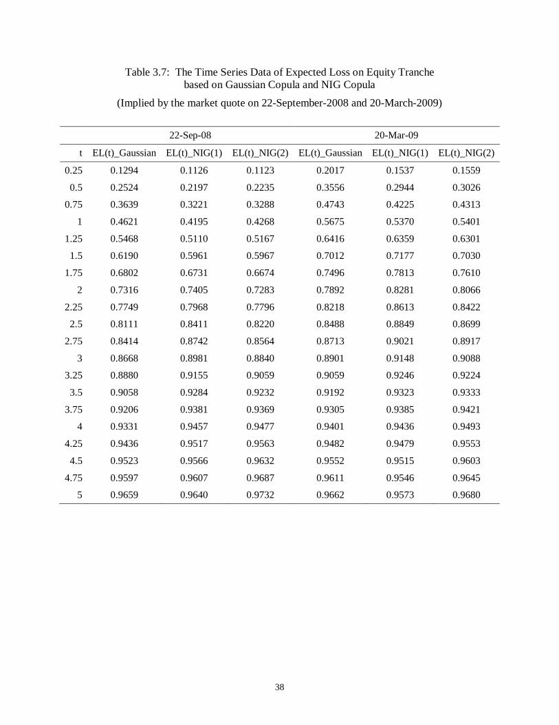
Table 3.7: The Time Series Data of Expected Loss on Equity Tranche

1
1 Introduction
In early 1990s when financial institutions such as banks were still the dominant players of
the market, credit derivatives e.g. credit default swap (CDS) and collateralized debt
obligation (CDO) were mainly used as a powerful risk management tool to mitigate the
credit exposure associated with the lending transactions. Although it remained the
ostensible purpose of creating this type of activities, gradually more and more hedge
funds and individual asset managers saw the arbitrage opportunities and began to
speculate. In 1999, the International Swap and Derivatives Association (ISDA) issued the
Credit Derivatives Definition and standardized the CDS contract. Since then we could see
a dramatic growth of the credit derivative market; the notional amount of the outstanding
contracts almost doubled from $ 34.2 trillion at 2006 year-end to $62.3 trillion dollars at
2007 year-end1, and among all the credit derivative products, index trades and synthetic
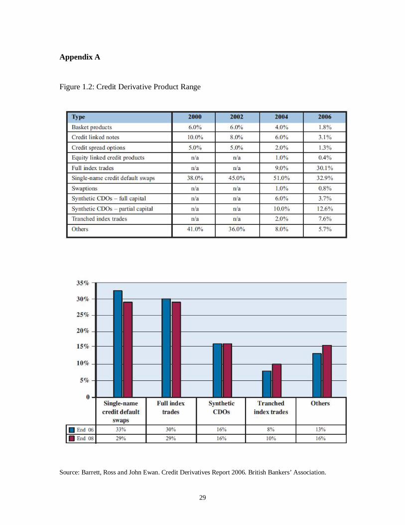
CDOs together have taken up 46% of the market. (Refer to Appendix A: Figure 1.2)
1 Source: Reuters: FACTBOX - Credit derivatives market in facts, figures. Feb.5, 2009.
(http://www.reuters.com/article/idUSL544102220090205)
Figure 1.1: Global Credit Derivative Market
0
10
20
30
40
50
60
70
2001 2002 2003 2004 2005 2006 2007 2008
Year-end Outstanding Contractsbased on Notional Amounts ($' trillion)
Source: Reuters
2
Unlike the value of financial instruments such as equity stocks and options, the value of a
CDO is largely determined by credit risk. Based on different valuation criteria we could
manually divide CDOs into two types, cash CDO and synthetic CDO. The underlying
assets of cash CDO are usually fixed income securities with less liquidity. We cannot
observe the debtor’s default probability from market quotes; therefore the valuation
process relies heavily on the rating agencies. A synthetic CDO is a portfolio of CDS. It is
structured in a way that default losses on the portfolio are allocated to tranches2, and the
debtor’s default probability of synthetic CDO could be implied from market quotes. This
gives such instrument an apparent advantage over cash CDO. In this paper, we only
consider the pricing model for synthetic CDOs.
From the quantitative perspective, how to account for the default loss distribution of the
whole credit portfolio is critical for the valuation process. Sophisticated numerical
techniques such as Monte Carlo simulation were used in order to fit the loose
assumptions. Ever since Gaussian Copula, a semi-analytical approach of CDO pricing
model, was introduced by Li (2000), it has been widely adopted by market practitioners.
This formula allows people to build unbelievable structures into the market. Its simplicity
and computational efficiency therefore made the model as the industrial standard.
However, the limitations of Gaussian Copula were hardly concerned. In late 2007, the
financial market began to behave beyond the model’s expectation, and high-risk credit
derivatives which were widely held by all kinds of financial institutions in the U.S.
subprime mortgage market quickly became worthless. Li’s model was then blamed as a
2 Hull, J., Options, Futures, and Other Derivatives, 7th edn. New Jersey: Pearson Prentice Hall, 2009, pp.
532.
3
“recipe for disaster”3: typically, (1) it does not consider the dynamic changes of the
debtor’s credit situation when calculating the expected loss distribution of the portfolio,
and (2) it cannot fit the fat tail feature of the loss distribution. Therefore, when we
calculate the implied correlation using market quote of different tranches of the same
CDO, we could observe the “correlation smile” phenomena.
In this paper we elaborate on an amended synthetic CDO pricing model based on a more
fat-tailed distribution assumption called Normal Inverse Gaussian distribution. The
structure of the paper is as follows: In Section One we conduct a brief literature review
on synthetic CDO pricing models. Followed by a short summary of the general semi-
analytical approach and the large homogeneous portfolio (LHP) assumption, we then
present the pricing formulas using one factor Gaussian Copula and NIG Copula models
respectively. The third section shows the estimated results as well as the comparative
analysis of the two models. Conclusion is finally summarized in the last section.
1.1 Literature Review
Currently there are primarily three methods to amend the standard one-factor CDO
pricing model. The first one is to extend the model by adding further stochastic factors.
Andersen and Sidenius (2005) believed that the correlation between debtors was a
stochastic process. It therefore used the random factor loading (RFL) model, and also
tested the spread payment of different tranches using random recovery rate. The second
one is to describe the correlation structure by using different copula functions, for
example, Schönbucher and Schubert (2001), Laurent and Gregory (2005), Schloegl and
3 Salmon, F, “Recipe for Disaster: The Formula That Killed Wall Street”, Wired Magazine, March 2009.

4
O’Kane (2005) used Student t-copula; Hull and White (2006) employed an implied
copula approach, which was a backward computation of conditional default probability
and hence the correlation structure using available market quote. The third one is to
replace the normal distribution assumption in the standard copula with other fat-tailed
distributions. Typical examples include double-t distribution in Hull and White (2004),
the one-factor heavy-tailed copula in Wang, Rachev and Fabozzi (2007). Burtschell,
Gregory and Laurent (2009) conducted a comparative analysis of the pricing efficiency of
standard Gaussian Copula, Student t-Copula, Double t-Copula, Clayton Copula,
Marshall-Olkin Copula and two RFL models. They concluded that the modeling outcome
of Double t-Copula and two RFL models were closer to the market quote of synthetic
CDO, and also solved the “correlation smile” better than other models.
However, due to the instability of the double-t distribution4 under convolution5, the
pricing formula of synthetic CDO cannot be solved analytically. Instead, additional
numerical methods have to be applied in order to calculate the quantiles of the
distribution, i.e. the default thresholds. Recently, the generalized hyperbolic distribution
(GH) has been introduced into CDO pricing models. Common forms include Normal
Inverse Gaussian (NIG) distribution in Kalemanova, Schmid and Werner (2007),
Variance Gamma distribution in Moosbrucker (2006), GH distribution in Eberlein and
Frey (2007). Particularly NIG distribution, which was first introduced in the field of
financial modeling by Brandorff-Nielsen (1997), has already been widely used in the
industrial practice. Its two special characteristics made it very suitable for CDO pricing:
4 It can also be called as bivariate t distribution. 5 Convolution is a mathematical operation on two functions, producing a third function that is typically
viewed as a modified version of one of the original functions.

5
(1) it can reflect the tail-heaviness and asymmetry using two parameters; and (2) it is
stable under convolution so that numerical computation could be significantly reduced.
Kalemanova, Schmid and Werner (2007) compared modeling results using Gaussian
Copula, Double t-Copula with degrees of freedom of 3 and 4, NIG Copula with one and
two free parameters. They then concluded that the standardized symmetric NIG
distribution fit CDO second tranche exactly, while the skewed NIG distribution with two
free parameters brought only a very slight improvement.
1.2 Purpose of the Paper
In this paper, we follow the philosophy in Kalemanova et al (2007) and define the pricing
efficiency as the size of the absolute error between modeling outcome and actual market
quote of all CDO tranches. The major purpose of this paper is to assess the pricing
efficiency of both Gaussian Copula and NIG Copula Model during the turbulent market
condition in 2008 and 2009, to see whether the conclusion in Kalemanova et al (2007)
still holds. Furthermore, we aim to examine the price impact of the skewed NIG
distribution by adjusting the value of the two free parameters.
6
2 Modeling
In this section, we present the modeling process of synthetic CDO pricing. Following the
steps in Kalemanova et al (2007), we first show the general semi-analytic approach for
synthetic CDO pricing, and the critical assumption of Large Homogeneous Portfolio
(LHP) Model. Then in the section of One Factor Copula Model, we take Gaussian Copula
for instance to derive the tranche expected loss. Normal Inverse Gaussian is discussed in
the end as an alternative distribution assumption.
2.1 General Semi-analytic Approach for Synthetic CDO Pricing
Basically, the purpose of pricing a synthetic CDO is to determine the fair value of each
tranche in the same structure. The protection buyer of CDO tranche pays periodic spread
payments to the protection seller at pre-settled payment dates, and the spread payment is
determined by the outstanding notional principal of each tranche. In case of a default
event, the compensation will be paid on the loss due to default event to the protection
buyer.
Suppose that are payment dates with and . and are the
attachment and detachment points of the tranche, which means this tranche is responsible
to cover the portfolio loss from to . With the assumption that interest rate, , is
constant, the discount factor is:
(1)
7
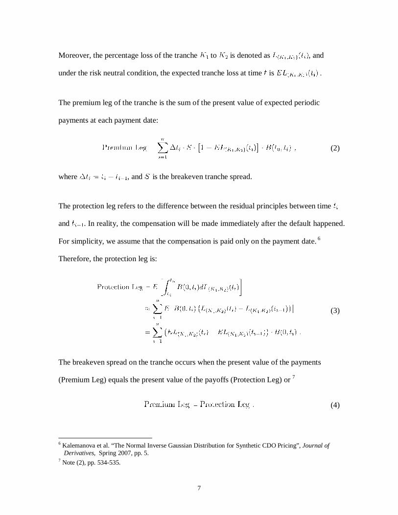
Moreover, the percentage loss of the tranche to is denoted as , and
under the risk neutral condition, the expected tranche loss at time is .
The premium leg of the tranche is the sum of the present value of expected periodic
payments at each payment date:
(2)
where , and is the breakeven tranche spread.
The protection leg refers to the difference between the residual principles between time
and . In reality, the compensation will be made immediately after the default happened.
For simplicity, we assume that the compensation is paid only on the payment date. 6
Therefore, the protection leg is:
(3)
The breakeven spread on the tranche occurs when the present value of the payments
(Premium Leg) equals the present value of the payoffs (Protection Leg) or 7
(4)
6 Kalemanova et al. “The Normal Inverse Gaussian Distribution for Synthetic CDO Pricing”, Journal of
Derivatives, Spring 2007, pp. 5. 7 Note (2), pp. 534-535.

8
Therefore the breakeven spread of the tranche covering the portfolio loss of to is:
(5)
In order to calculate tranche spread in Eq.(5), we need the series of tranche expected loss
at each the payment date.
When the portfolio suffer a loss of L(ti), the corresponding loss of the tranche to is:
(6)
If the continuous portfolio loss distribution function, , is given, then the expected
loss on the tranche is:
(7)
Thus, the central problem in the pricing of a CDO tranche is to derive the loss distribution
of the reference portfolio.8
2.2 Large Homogeneous Portfolio Assumption
During the estimation process of the continuous portfolio loss distribution function, it is
critical to assume that the reference portfolio is composed by infinite number of
8 Note (4), pp. 6.

9
homogeneous assets with the same pairwise default correlation. Then the portfolio has
follow traits:
a) The unsystematic risk of the reference portfolio is diversified away because of the
infinite number of the underlying assets.
b) All the underlying assets in the portfolio are equally weighted and share the same
spread and recovery rate.
c) The default dependence structure follows the One Factor Copula Model, whose
form is characterized by different distribution assumptions.
d) The pairwise default correlation is constant for the whole structure, so that the
correlation can be implied from equity tranche to price other mezzanine tranches
and senior tranches.
2.3 One Factor Gaussian Copula Model
The LHP approach is based on a One Factor Gaussian Copula Model of correlated
defaults.9 It has been approved that One Factor Copula Model is useful in describing the
joint default probability among different credit entities. One Factor Gaussian Copula
Model was introduced by Li (1999, 2000), and then was developed as the market standard
model. The following section shows how to derive the loss distribution of the reference
portfolio by using this model.
9 Note (4), pp. 7.
10
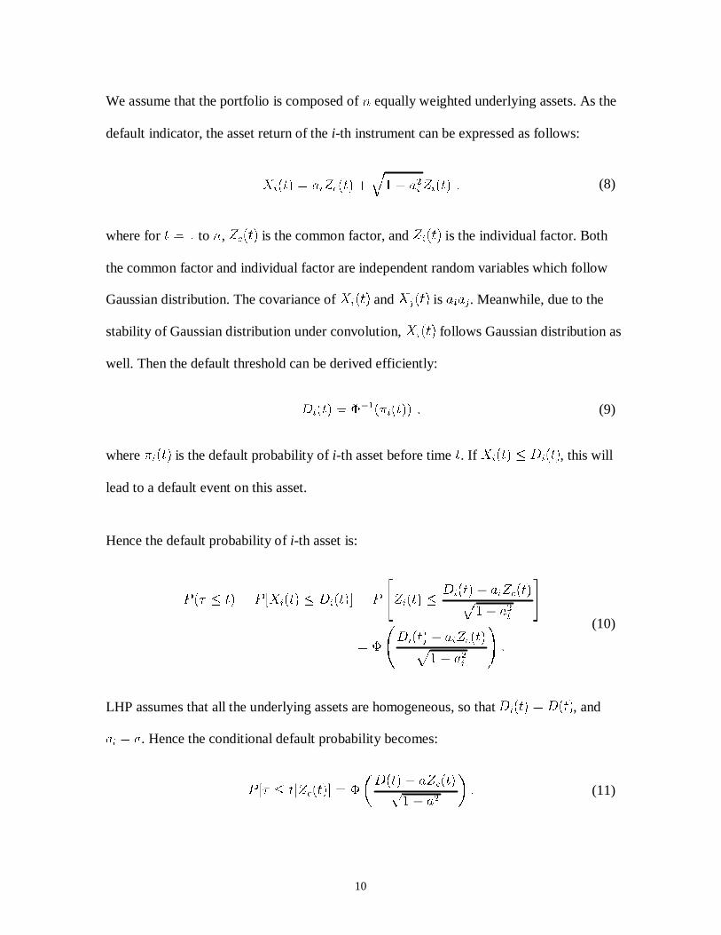
We assume that the portfolio is composed of equally weighted underlying assets. As the
default indicator, the asset return of the i-th instrument can be expressed as follows:
(8)
where for to , is the common factor, and is the individual factor. Both
the common factor and individual factor are independent random variables which follow
Gaussian distribution. The covariance of and is . Meanwhile, due to the
stability of Gaussian distribution under convolution, follows Gaussian distribution as
well. Then the default threshold can be derived efficiently:
(9)
where is the default probability of i-th asset before time . If , this will
lead to a default event on this asset.
Hence the default probability of i-th asset is:
(10)
LHP assumes that all the underlying assets are homogeneous, so that , and
. Hence the conditional default probability becomes:
(11)
11
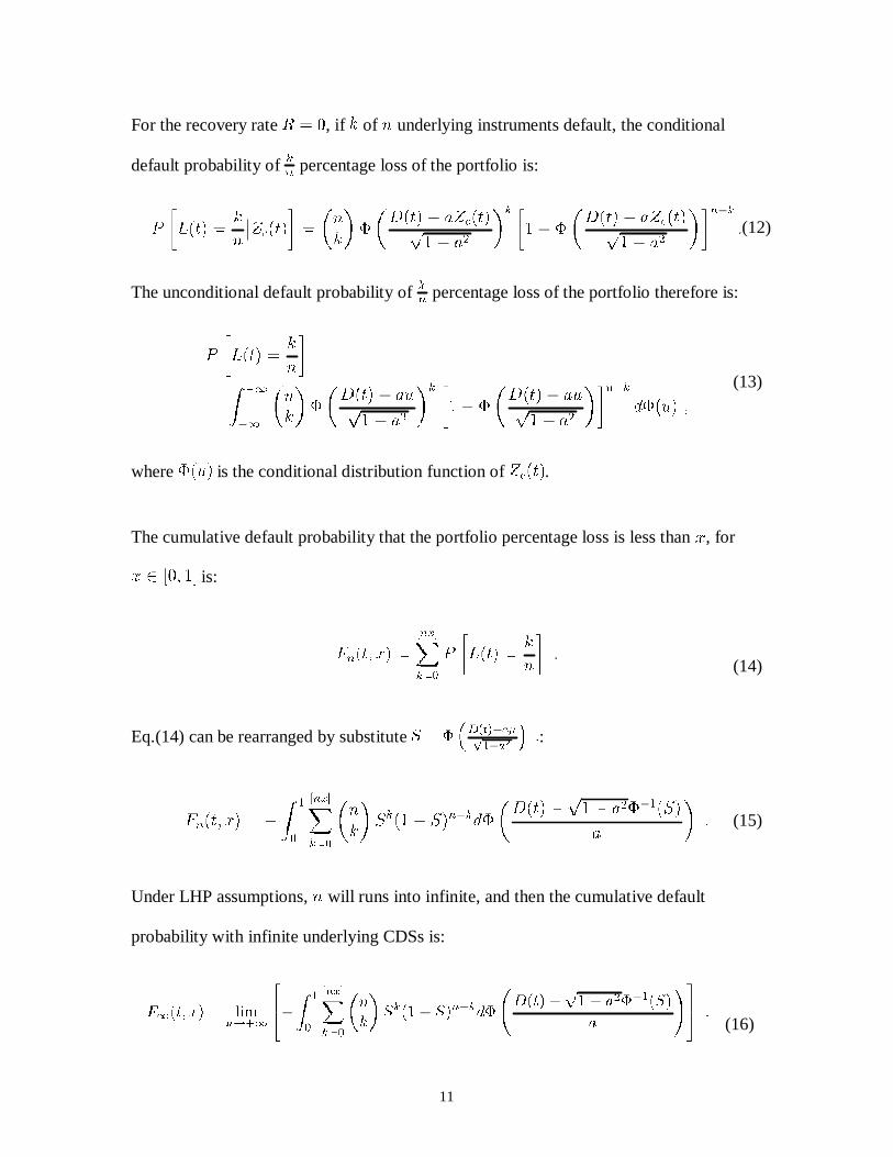
For the recovery rate , if of underlying instruments default, the conditional
default probability of percentage loss of the portfolio is:
(12)
The unconditional default probability of percentage loss of the portfolio therefore is:
(13)
where is the conditional distribution function of .
The cumulative default probability that the portfolio percentage loss is less than , for
is:
(14)
Eq.(14) can be rearranged by substitute :
(15)
Under LHP assumptions, will runs into infinite, and then the cumulative default
probability with infinite underlying CDSs is:
(16)
12
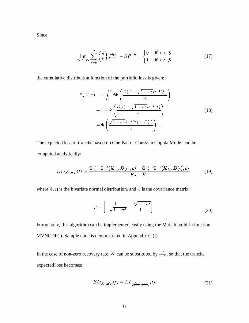
Since
(17)
the cumulative distribution function of the portfolio loss is given:
(18)
The expected loss of tranche based on One Factor Gaussian Copula Model can be
computed analytically:
(19)
where is the bivariate normal distribution, and is the covariance matrix:
(20)
Fortunately, this algorithm can be implemented easily using the Matlab build-in function
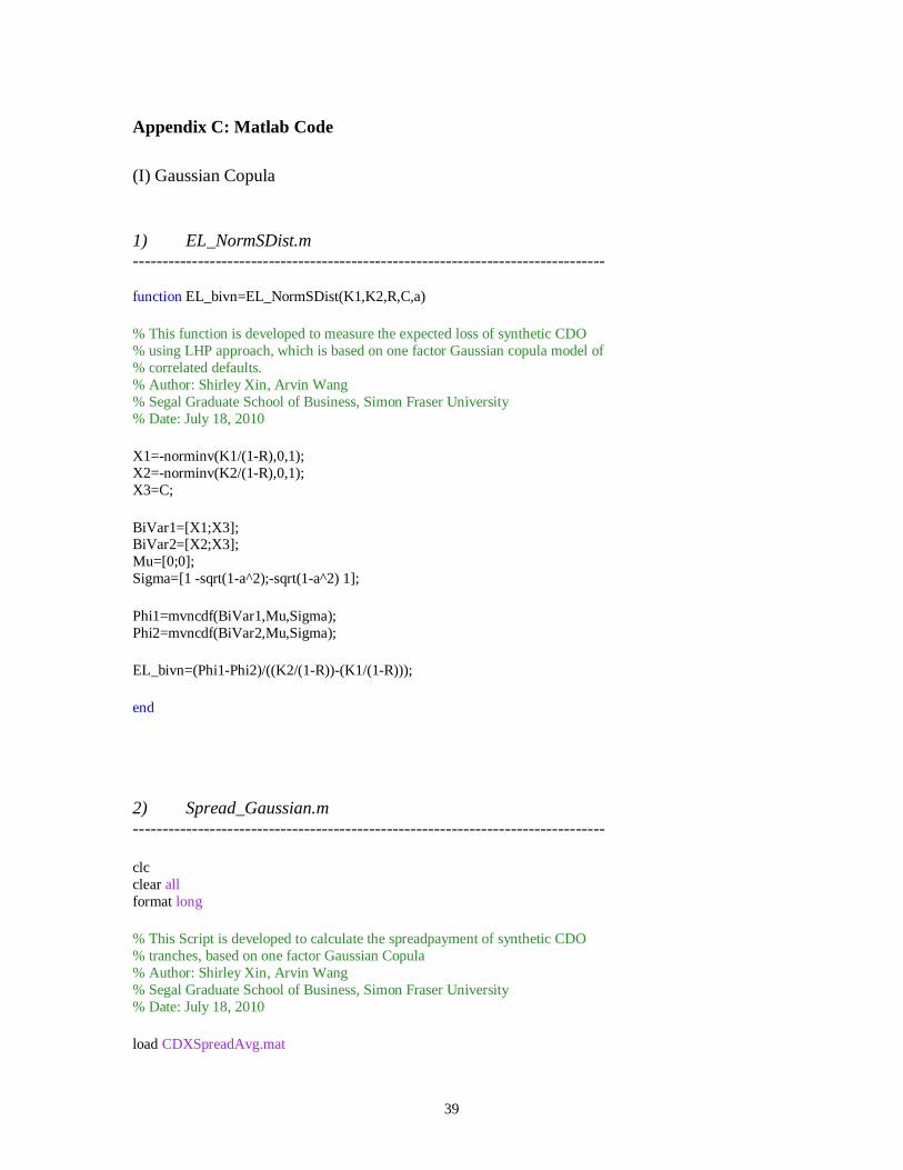
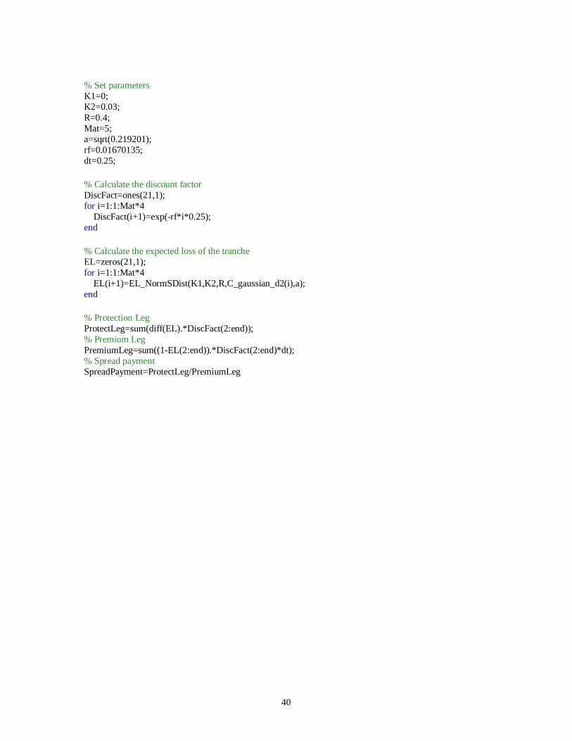
MVNCDF( ). Sample code is demonstrated in Appendix C (I).
In the case of non-zero recovery rate, can be substituted by , so that the tranche
expected loss becomes:
(21)
13
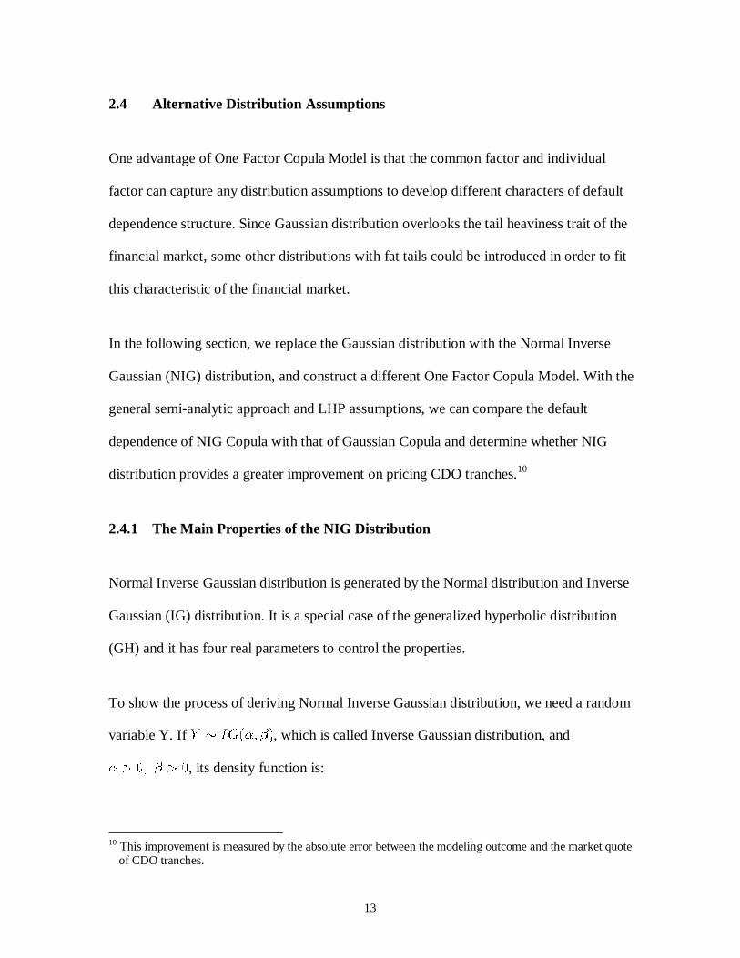
2.4 Alternative Distribution Assumptions
One advantage of One Factor Copula Model is that the common factor and individual
factor can capture any distribution assumptions to develop different characters of default
dependence structure. Since Gaussian distribution overlooks the tail heaviness trait of the
financial market, some other distributions with fat tails could be introduced in order to fit
this characteristic of the financial market.
In the following section, we replace the Gaussian distribution with the Normal Inverse
Gaussian (NIG) distribution, and construct a different One Factor Copula Model. With the
general semi-analytic approach and LHP assumptions, we can compare the default
dependence of NIG Copula with that of Gaussian Copula and determine whether NIG
distribution provides a greater improvement on pricing CDO tranches.10
2.4.1 The Main Properties of the NIG Distribution
Normal Inverse Gaussian distribution is generated by the Normal distribution and Inverse
Gaussian (IG) distribution. It is a special case of the generalized hyperbolic distribution
(GH) and it has four real parameters to control the properties.
To show the process of deriving Normal Inverse Gaussian distribution, we need a random
variable Y. If , which is called Inverse Gaussian distribution, and
, its density function is:
10 This improvement is measured by the absolute error between the modeling outcome and the market quote
of CDO tranches.
14
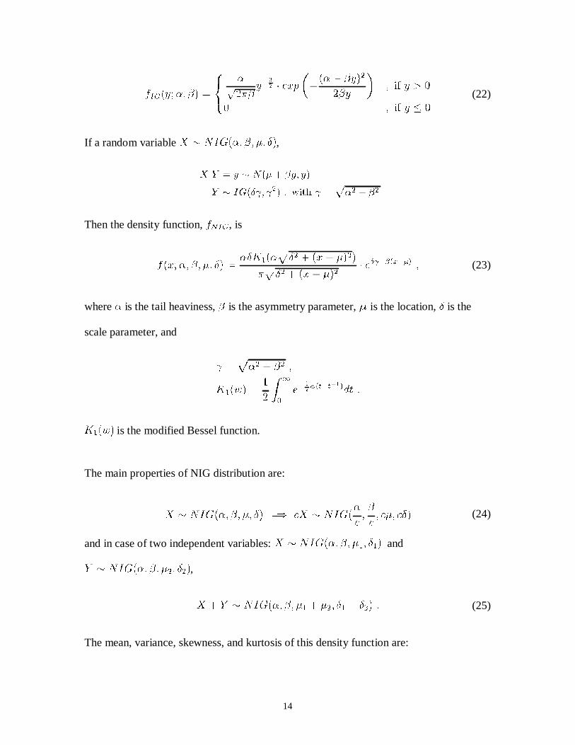
(22)
If a random variable ,
Then the density function, , is
(23)
where is the tail heaviness, is the asymmetry parameter, is the location, is the
scale parameter, and
is the modified Bessel function.
The main properties of NIG distribution are:
(24)
and in case of two independent variables: and
,
(25)
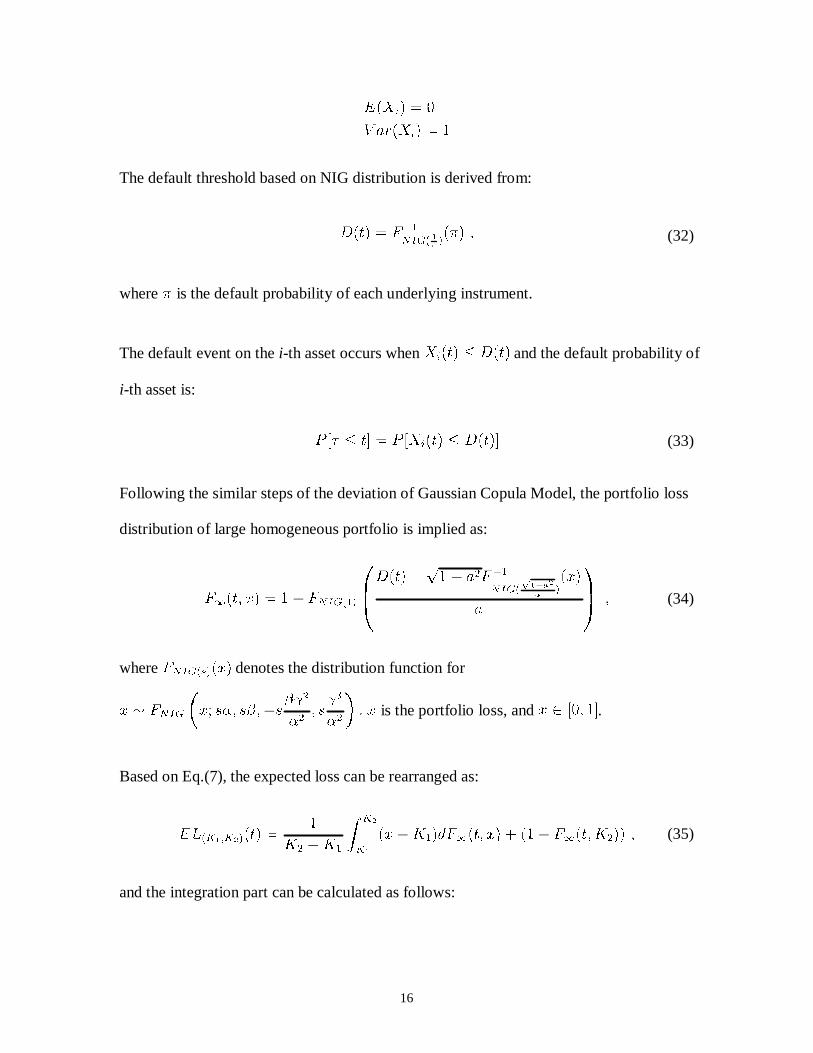
The mean, variance, skewness, and kurtosis of this density function are:

15
2.4.2 The NIG Copula Model with LHP Assumption
To form NIG Copula Model, the asset return, , is required to follow the standard NIG
distribution, which has the zero mean and unit variance. The common factor and
individual factor in Copula Model are of the following forms:
(26)
(27)
Then we have:
(28)
(29)
Since
(30)
and with the property of NIG distribution under convolution (refer to Eq.(24) and Eq.(25)),
is derived as:
(31)
whose mean and variance are:
16
The default threshold based on NIG distribution is derived from:
(32)
where is the default probability of each underlying instrument.
The default event on the i-th asset occurs when and the default probability of
i-th asset is:
(33)
Following the similar steps of the deviation of Gaussian Copula Model, the portfolio loss
distribution of large homogeneous portfolio is implied as:
(34)
where denotes the distribution function for
is the portfolio loss, and .
Based on Eq.(7), the expected loss can be rearranged as:
(35)
and the integration part can be calculated as follows:
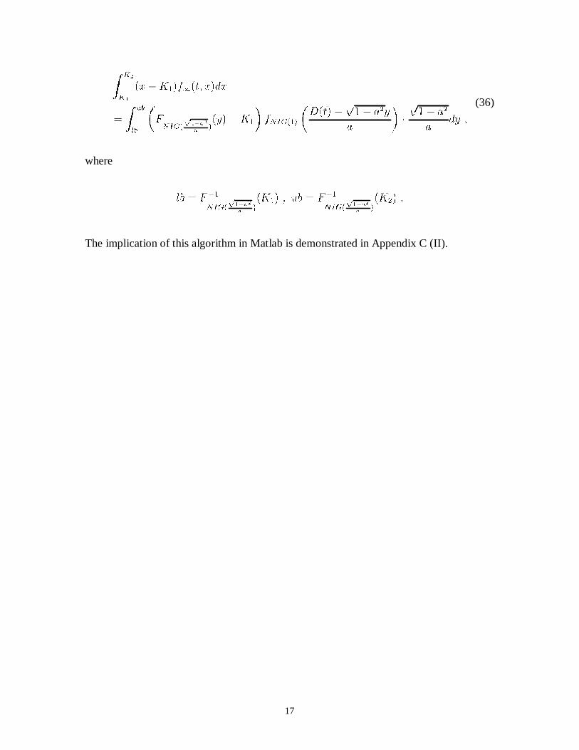
17
(36)
where
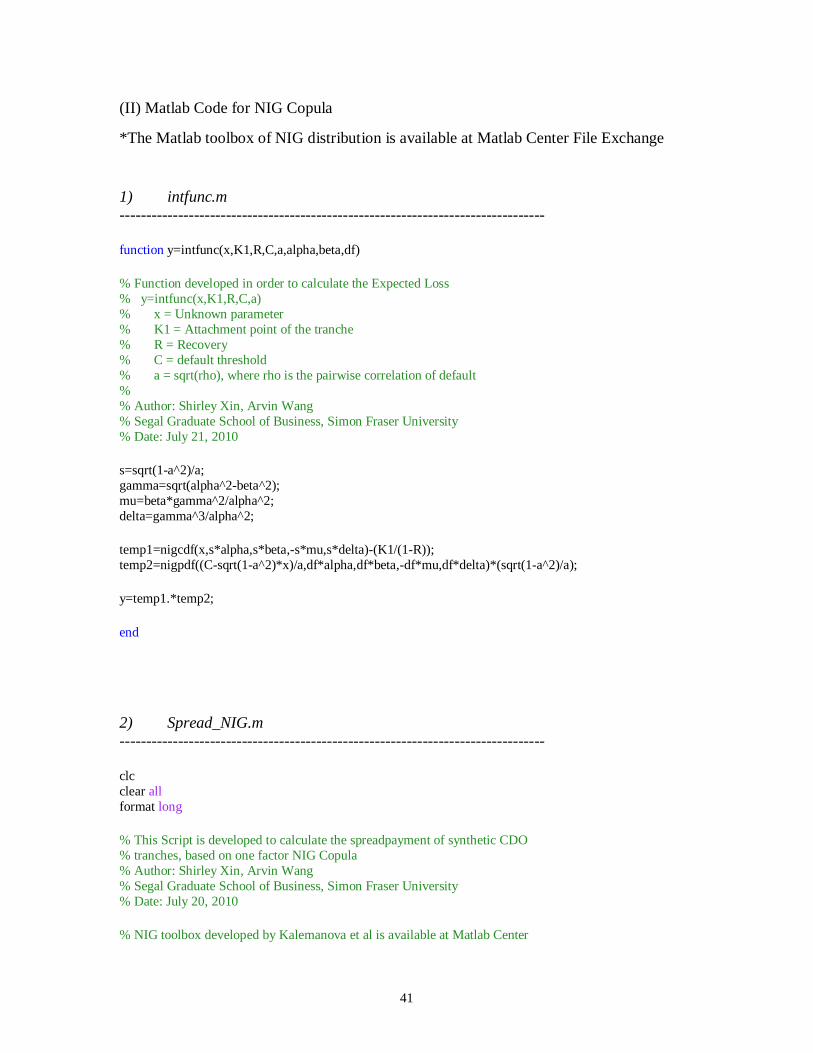
The implication of this algorithm in Matlab is demonstrated in Appendix C (II).
18
3 Market Data
In this paper, 5-year Dow Jones CDX.NA.IG index is employed in order to compare the
effects of different distribution assumptions on test results. CDX family contains North
American and Emerging Market companies. It is a standardized index, which is
composed by 125 equally weighted CDSs of investment grade entity. The successive
tranches have attachment or detachment points at 0%, 3%, 7%, 10%, 15%, and 30%. All
the underlying CDSs are assumed to share the same recovery rate and default probability,
which are consistent with the index.
The ninth series of Dow Jones CDX.NA.IG index has the effective date on 21-
September-2007 and the maturity date on 20-December-2012, and rolls every 6 months in
March and September. The market quote of this CDS index portfolio is 156.5 basis points
on 22-September-2008 and is 271.0 basis points on 20-March-2009.
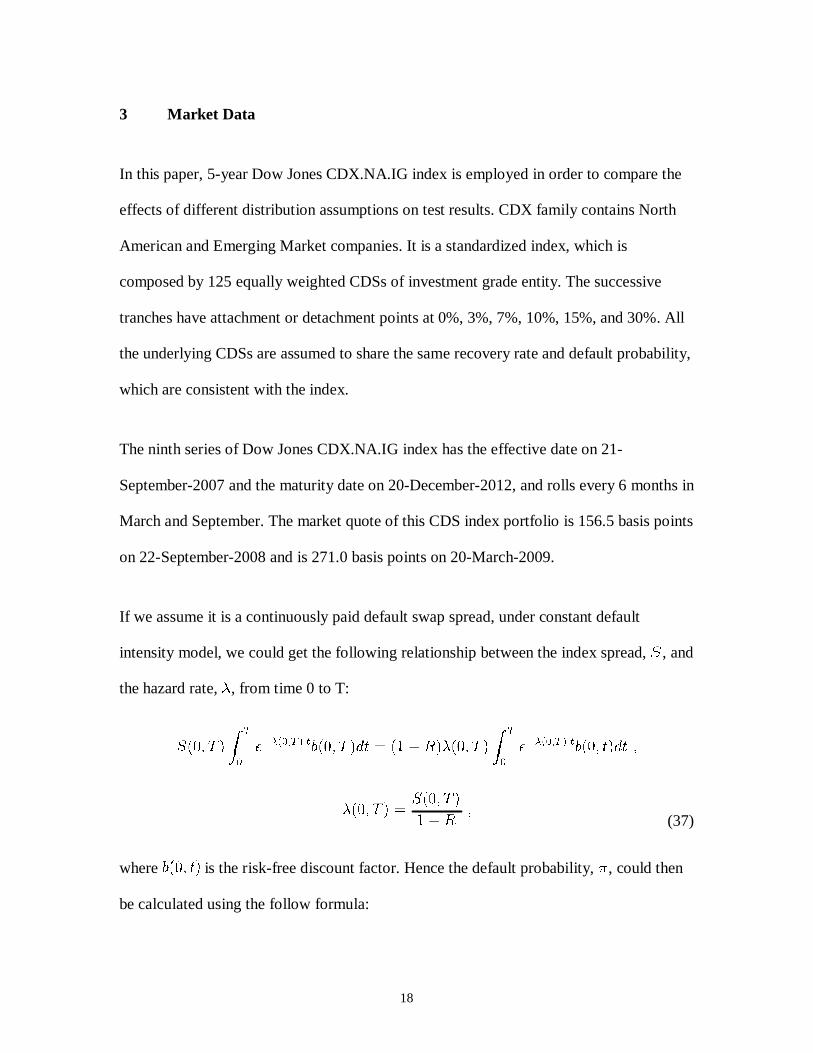
If we assume it is a continuously paid default swap spread, under constant default
intensity model, we could get the following relationship between the index spread, , and
the hazard rate, , from time 0 to T:
(37)
where is the risk-free discount factor. Hence the default probability, , could then
be calculated using the follow formula:
19
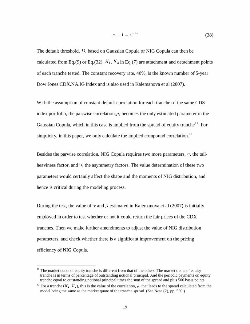
(38)
The default threshold, , based on Gaussian Copula or NIG Copula can then be
calculated from Eq.(9) or Eq.(32). , in Eq.(7) are attachment and detachment points
of each tranche tested. The constant recovery rate, 40%, is the known number of 5-year
Dow Jones CDX.NA.IG index and is also used in Kalemanova et al (2007).
With the assumption of constant default correlation for each tranche of the same CDS
index portfolio, the pairwise correlation, , becomes the only estimated parameter in the
Gaussian Copula, which in this case is implied from the spread of equity tranche11. For
simplicity, in this paper, we only calculate the implied compound correlation.12
Besides the parwise correlation, NIG Copula requires two more parameters, , the tail-
heaviness factor, and , the asymmetry factors. The value determination of these two
parameters would certainly affect the shape and the moments of NIG distribution, and
hence is critical during the modeling process.
During the test, the value of and estimated in Kalemanova et al (2007) is initially
employed in order to test whether or not it could return the fair prices of the CDX
tranches. Then we make further amendments to adjust the value of NIG distribution
parameters, and check whether there is a significant improvement on the pricing
efficiency of NIG Copula.
11 The market quote of equity tranche is different from that of the others. The market quote of equity
tranche is in terms of percentage of outstanding notional principal. And the periodic payments on equity tranche equal to outstanding notional principal times the sum of the spread and plus 500 basis points.
12 For a tranche ( ), this is the value of the correlation, , that leads to the spread calculated from the model being the same as the market quote of the tranche spread. (See Note (2), pp. 539.)

20
In NIG (1), besides the pairwise correlation , we only have one free parameter , and
, which means this is a standard symmetric NIG distribution. To test the effect of
the skewness of NIG distribution on the pricing efficiency of the model, NIG (2) is
introduced. NIG (2) frees the second parameter , therefore is a more generalized skewed
NIG distribution.
3.1 Modeling Outcome and Comparative Analysis
3.1.1 Validation of the Estimation in Kalemanova et al (2007)
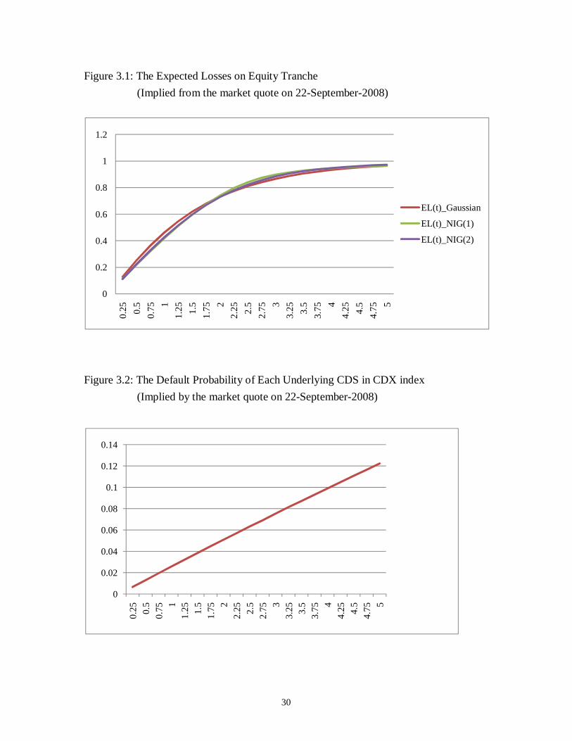
As we can see, in Appendix A: Figure 3.1 the expected loss of the equity tranche (in term
of percentage loss of the reference portfolio) on 22-September-2008 increases through
time and becomes smooth when the time is close to maturity date. The increasing trend of
the expected loss is consistent with the corresponding default probability of each
underlying CDS (refer to Appendix A: Figure 3.2). However, the Gaussian Copula
overlooked the fat tail trait of the financial market. The expected loss based on Gaussian
Copula is higher than those based on NIG Copulas at the beginning, after all the expected
losses intersect when time lies between 1.75 years to 2 years, the expected loss based on
Gaussian Copula is among the lowest comparing with the two NIG Copulas. With the
increase of the tail heaviness, the expected loss becomes higher when time is close to
maturity. This phenomenon of the expected loss and corresponding default probability on
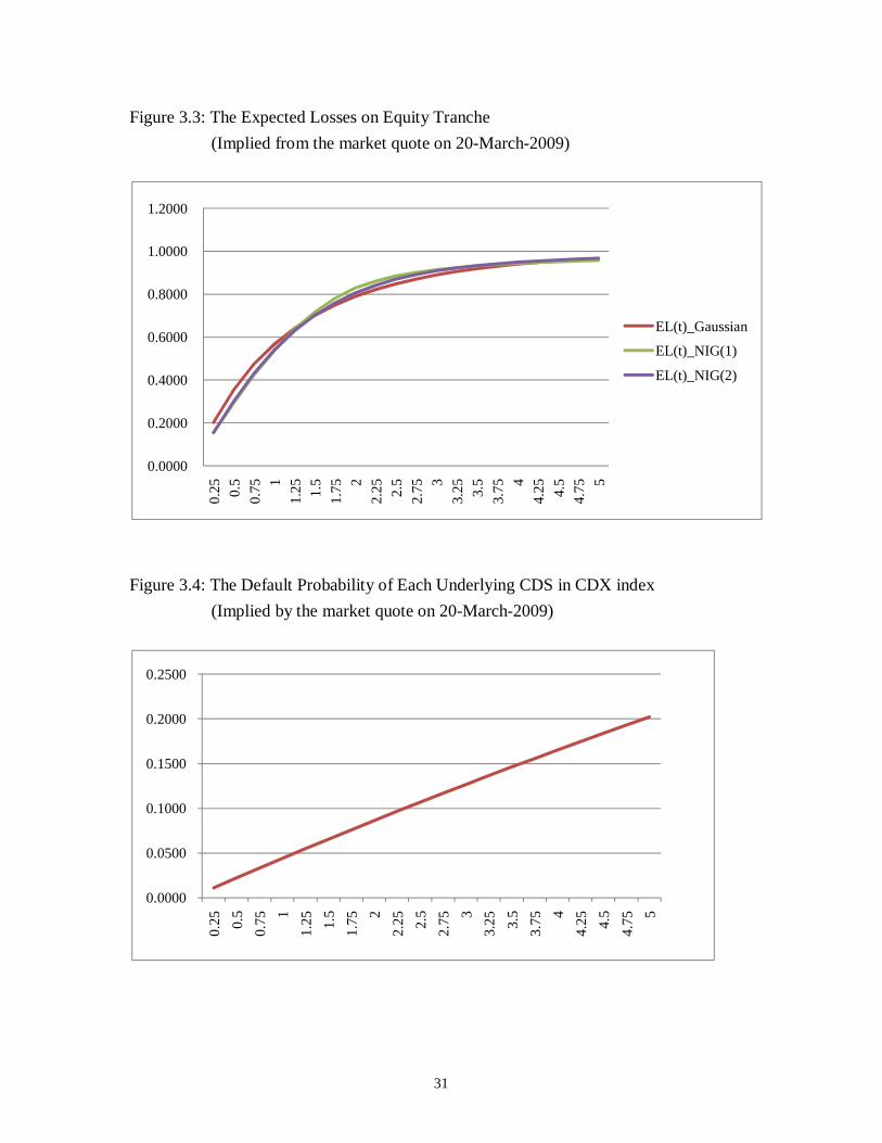
22-September-2008 is similar to that on 20-March-2009 (refer to Appendix A: Figure 3.3
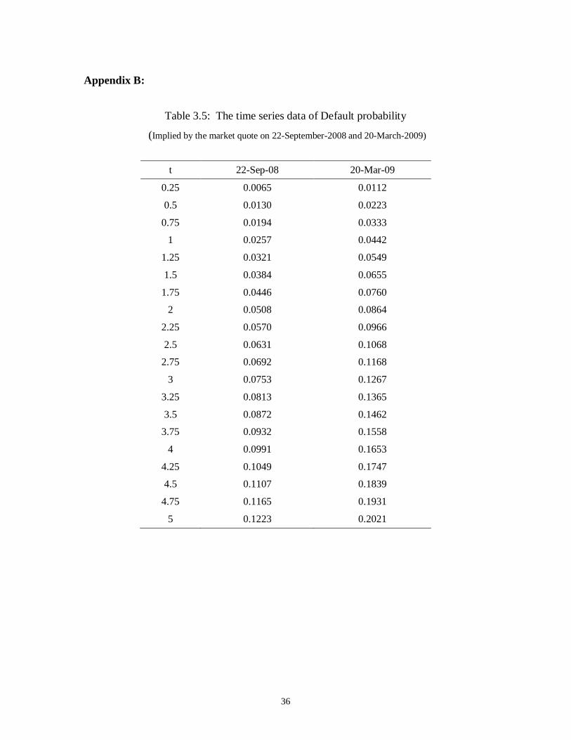
and Figure 3.4). Appendix B: Table 3.5 to Table 3.7 present further detailed data of the
default probability of each underlying CDS in the reference portfolio, the default
threshold, and the expected loss of the equity tranche.

21
Table 3.1 shows the comparison of market quotes on 22-September-2008 to the outputs of
each model. In general, the Gaussian Copula and the two NIG Copulas all overprice the
mezzanine tranches, and underprice the senior tranche. Comparing with the Gaussian
Copula, the two NIG Copula models return more accepted test result based on the size of
the absolute error. The introduction of in NIG (2) doesn’t bring so much improvement to
the test result; it only shows a slightly better fit on the second tranche. Despite the fact that
the pricing efficiency of NIG copula is improved for the whole structure of the CDS index
portfolio, we find 89.91% of the error in NIG (1) is resulted from the second tranche, and
that in NIG (2) is 76.65%. Using the same parameter values on NIG (1) and NIG (2) in
Kalemanova et al (2007), the overprice on second tranche is completely against their
conclusion, which is that NIG Copula could exactly match the market quote of the second
tranche.
Table 3.1: The Market Quote and Modeling Outcome of Each Tranche
22-September-2008 (bp)
Market Quote13
Gaussian NIG(1) NIG(2)
CDX Index 156.5000
0-3% 65.7950% 65.7950% 65.7950% 65.7950%
3-7% 869.5000 1886.7908 1703.6568 1614.6424
7-10% 395.5100 724.2516 462.3443 549.6528
10-15% 187.5550 250.3531 190.4495 245.5106
15-30% 91.7650 22.3734 67.9534 76.8759
Absolute Error 1478.2222 927.6972 972.1300
Rho
0.110107 0.189630 0.199591
Alpha
0.4794 0.6020
Beta 0 -0.1605
13 Source from: Bloomberg.
22
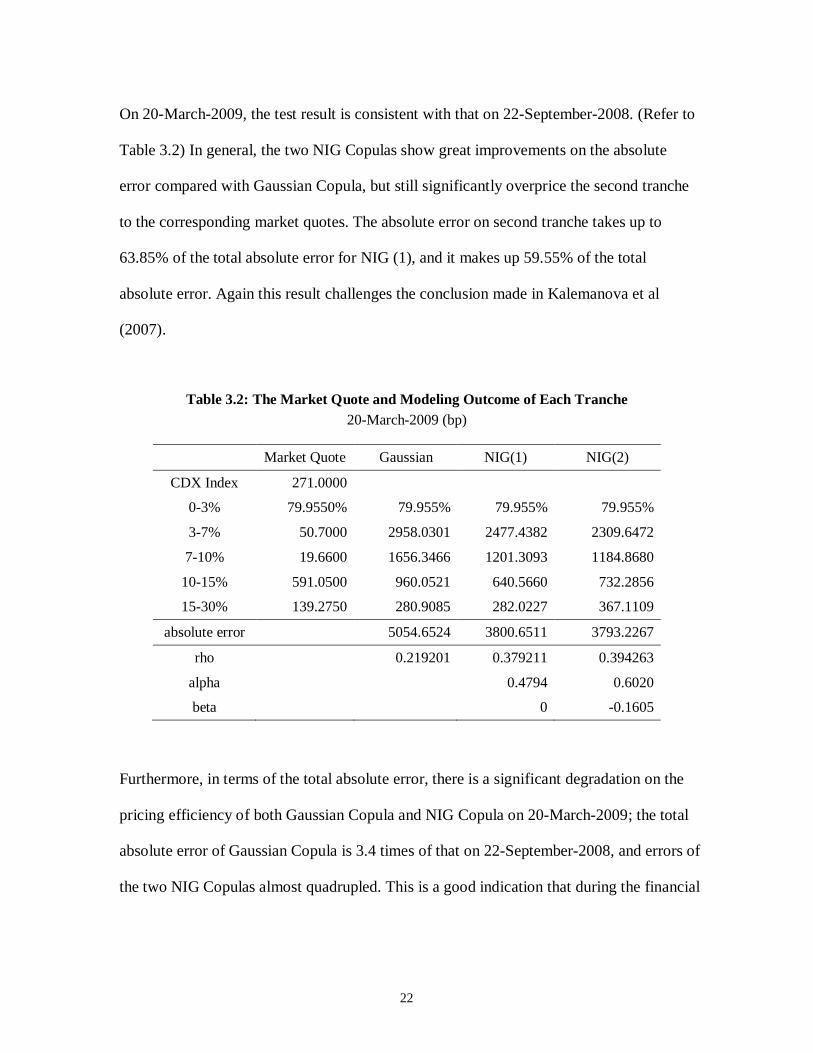
On 20-March-2009, the test result is consistent with that on 22-September-2008. (Refer to
Table 3.2) In general, the two NIG Copulas show great improvements on the absolute
error compared with Gaussian Copula, but still significantly overprice the second tranche
to the corresponding market quotes. The absolute error on second tranche takes up to
63.85% of the total absolute error for NIG (1), and it makes up 59.55% of the total
absolute error. Again this result challenges the conclusion made in Kalemanova et al
(2007).
Table 3.2: The Market Quote and Modeling Outcome of Each Tranche
20-March-2009 (bp)
Market Quote Gaussian NIG(1) NIG(2)
CDX Index 271.0000
0-3% 79.9550% 79.955% 79.955% 79.955%
3-7% 50.7000 2958.0301 2477.4382 2309.6472
7-10% 19.6600 1656.3466 1201.3093 1184.8680
10-15% 591.0500 960.0521 640.5660 732.2856
15-30% 139.2750 280.9085 282.0227 367.1109
absolute error 5054.6524 3800.6511 3793.2267
rho 0.219201 0.379211 0.394263
alpha 0.4794 0.6020
beta 0 -0.1605
Furthermore, in terms of the total absolute error, there is a significant degradation on the
pricing efficiency of both Gaussian Copula and NIG Copula on 20-March-2009; the total
absolute error of Gaussian Copula is 3.4 times of that on 22-September-2008, and errors of
the two NIG Copulas almost quadrupled. This is a good indication that during the financial
23
crunch in 2008 and 2009, the market has reacted way beyond the models’ estimation
capacity. The industry is now in urgent need of further amendment.
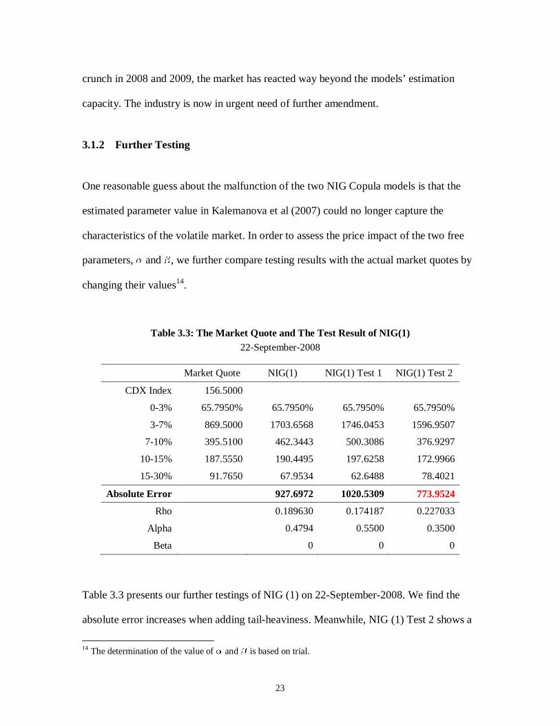
3.1.2 Further Testing
One reasonable guess about the malfunction of the two NIG Copula models is that the
estimated parameter value in Kalemanova et al (2007) could no longer capture the
characteristics of the volatile market. In order to assess the price impact of the two free
parameters, and , we further compare testing results with the actual market quotes by
changing their values14.
Table 3.3: The Market Quote and The Test Result of NIG(1)
22-September-2008
Market Quote NIG(1) NIG(1) Test 1 NIG(1) Test 2
CDX Index 156.5000
0-3% 65.7950% 65.7950% 65.7950% 65.7950%
3-7% 869.5000 1703.6568 1746.0453 1596.9507
7-10% 395.5100 462.3443 500.3086 376.9297
10-15% 187.5550 190.4495 197.6258 172.9966
15-30% 91.7650 67.9534 62.6488 78.4021
Absolute Error 927.6972 1020.5309 773.9524
Rho 0.189630 0.174187 0.227033
Alpha 0.4794 0.5500 0.3500
Beta 0 0 0
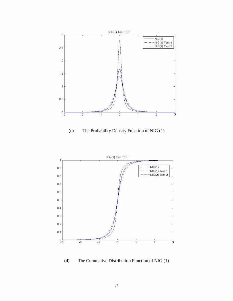
Table 3.3 presents our further testings of NIG (1) on 22-September-2008. We find the
absolute error increases when adding tail-heaviness. Meanwhile, NIG (1) Test 2 shows a
14 The determination of the value of and is based on trial.
24
significant improvement of the whole structure; the absolute error dropped 153.74 bp
when changed from 0.4794 to 0.35. The second tranche is now less overpriced, while
the senior tranche is less underpriced.
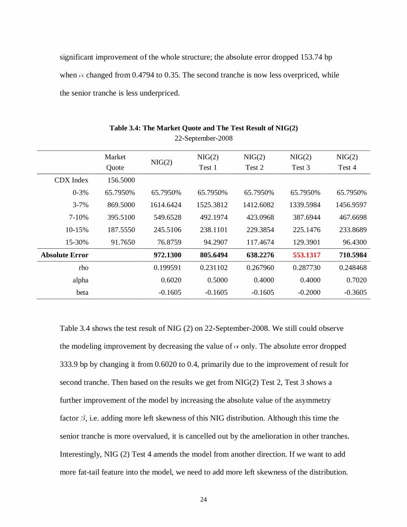
Table 3.4: The Market Quote and The Test Result of NIG(2)
22-September-2008
Market
Quote NIG(2)
NIG(2)
Test 1
NIG(2)
Test 2
NIG(2)
Test 3
NIG(2)
Test 4
CDX Index 156.5000
0-3% 65.7950% 65.7950% 65.7950% 65.7950% 65.7950% 65.7950%
3-7% 869.5000 1614.6424 1525.3812 1412.6082 1339.5984 1456.9597
7-10% 395.5100 549.6528 492.1974 423.0968 387.6944 467.6698
10-15% 187.5550 245.5106 238.1101 229.3854 225.1476 233.8689
15-30% 91.7650 76.8759 94.2907 117.4674 129.3901 96.4300
Absolute Error
972.1300 805.6494 638.2276 553.1317 710.5984
rho
0.199591 0.231102 0.267960 0.287730 0.248468
alpha
0.6020 0.5000 0.4000 0.4000 0.7020
beta
-0.1605 -0.1605 -0.1605 -0.2000 -0.3605
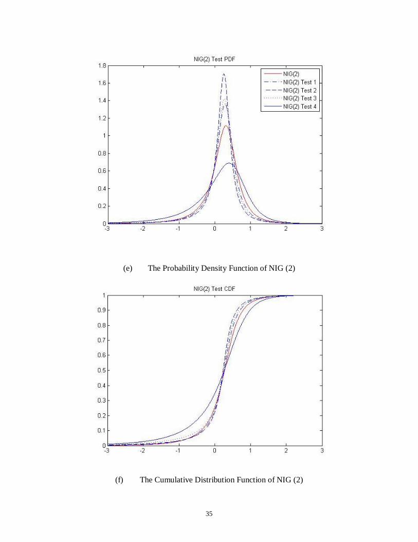
Table 3.4 shows the test result of NIG (2) on 22-September-2008. We still could observe
the modeling improvement by decreasing the value of only. The absolute error dropped
333.9 bp by changing it from 0.6020 to 0.4, primarily due to the improvement of result for
second tranche. Then based on the results we get from NIG(2) Test 2, Test 3 shows a
further improvement of the model by increasing the absolute value of the asymmetry
factor , i.e. adding more left skewness of this NIG distribution. Although this time the
senior tranche is more overvalued, it is cancelled out by the amelioration in other tranches.
Interestingly, NIG (2) Test 4 amends the model from another direction. If we want to add
more fat-tail feature into the model, we need to add more left skewness of the distribution.

25
This might be a reasonable clue showing that there is a non linear relationship between the
spread payment of the tranches and the parameter value of and .
There is a same phenomenon in test result of both NIG (1) and NIG (2): decreasing the
value of improves the modeling results of NIG Copula. In Table 3.3, the adjustment of
from 0.4794 to 0.3500 causes a decrease in absolute error from 927.6972 bp to 773.9524
bp. And in Table 3.4, by making fixed at -0.1605, we could observe that the change of
from 0.6020 to 0.4000 leads to the absolute error decrease dramatically from 972.1300 bp
to 638.2276 bp.
The difference between the market data used in this paper and that in Kalemanova et al
(2007) can be one possible explanation to the phenomenon that less fat tail feature
improves the result of both NIG (1) Copula and NIG (2) Copula. In Kalemanova et al
(2007), 5-year iTraxx Euro index is applied as the market data. This index is is composed
by 125 equally weighted CDSs of investment grade entities in Europe, rather than in North
America. And it is possible that Dow Jones CDX.NA.IG index portfolio has less fat tail
feature than that of iTraxx Euro index.

26
4 Conclusion
The main purpose of this paper is to compare the effect of NIG distribution to that of
Gaussian distribution on Synthetic CDO Pricing, and to further test the pricing efficiency
of One Factor Copula Model based on the skewed NIG distribution.
Basically, NIG Copula brings the fat tail trait into the model, and therefore it produces
better result to fit the market quote than Gaussian Copula. The standard NIG distribution
captured by One Factor Copula Model has two parameters to define its tail heaviness and
symmetry. Moreover, there is one advantage of NIG distribution: due to the stability of
NIG distribution under convolution, the computation of default threshold is time efficient.
In this paper, we employ the parameter value of NIG distribution estimated in Kalemanova
et al (2007), and get an unfavorable result on the second tranche. This differs from their
conclusion. By making further adjustments on the two parameters, we observe that
decreasing the tail heaviness and increasing the left skewness of NIG (2) lead to a
significant improvement to the test result. Therefore, the key issue about using NIG
Copula is how to estimate the tail heaviness and asymmetry of the NIG distribution.
For further development of this paper, there are at least two points should be considered:
1) how to determine the optimal value of the tail heaviness and asymmetry of the NIG
distribution to fit the market quote; 2) is the result sensitive to the value of the recovery
rate.
27
Reference:
[1] Andersen, L., and J. Sidenius, “Extensions to the Gaussian Copula: Random
Recovery and Random Factor Loadings”, Journal of Credit Risk, 2005, 1(1): 29-70.
[2] Barndorff-Nielsen, O., “Normal Inverse Gaussian Distributions and Stochastic
Volatility Modelling”, Sandinavian Journal of Statistics, 1997, 24: 1-13.
[3] Burtschell X., J. Gregory and J. Laurent, “A Comparative Analysis of CDO Pricing
Models”, Working paper, 2009, ISFA Actuarial School, University of Lyon and
BNP Paribas.
[4] Duffie, D., and K. Singleton, Credit Risk: Pricing, Measurement and Management.
New Jersey: Princeton University Press, 2003.
[5] Eberlein, E., and R. Frey, “Advanced Credit Portfolio Modeling and CDO Pricing”,
Working paper, 2007, University of Freiburg.
[6] Hull, J., Options, Futures, and Other Derivatives, 7th edn. New Jersey: Pearson
Prentice Hall, 2009, pp. 517-544.
[7] Hull, J., and A. White, “Valuation of a CDO and an nth to Default CDS Without
Monte Carlo Simulation”, Journal of Derivatives, 2004, 12(2): 8-23.
[8] Hull, J., and A. White, “Valuation Credit Derivatives Using an Implied Copula
Approach”, Journal of Derivatives, 2006, 14(2): 8-28.
[9] Kalemanova, A., B. Schmid and R. Werner, “The Normal Inverse Gaussian
Distribution for Synthetic CDO Pricing”, Journal of Derivatives, 2007.
[10] Laurent, J., and J. Gregory, “Basket Default Swaps, CDOs and Factor Copulas”,
Journal of Risk, 2005, 7(4): 8-23.
28
[11] Li, D., “On Default Correlation: A Copula Approach”, Journal of Fixed Income,
2000, 9: 43-54.
[12] Moosbrucher, T., “Pricing CDOs with Correlated Variance Gamma Distributions”,
Working Paper, 2006, Center for Financial Research, University of Cologne.
[13] O’Kane, D., and S. Turnbull, “Valuation of Credit Default Swaps”, Lehman
Brothers Quantitative Credit Research, Vol. 2003-Q1/Q2.
[14] Schloegl, L., and D. O’Kane, “A Note on the Large Homogeneous Portfolio
Approximation with the Student t Copula”, Finance and Stochastic, 2005, 9(4):
577-584.
[15] Schönbucher, P., Credit Derivatives Pricing Models. New York: Wiley, 2003.
[16] Schönbucher, P., and D. Schubert, “Copula Dependent Default Risk in Intensity
Models”, Working paper, 2001, Bonn University.
[17] Wang, D., S. Rachev and F. Fabozzi, “Pricing of Credit Default Index Swap
Tranches with One-Factor Heavy-Tailed Copula Models”, Working paper, 2007,
University of California, Santa Barbara.
29
Appendix A
Figure 1.2: Credit Derivative Product Range
Source: Barrett, Ross and John Ewan. Credit Derivatives Report 2006. British Bankers’ Association.
30
Figure 3.1: The Expected Losses on Equity Tranche
(Implied from the market quote on 22-September-2008)
Figure 3.2: The Default Probability of Each Underlying CDS in CDX index
(Implied by the market quote on 22-September-2008)
0
0.02
0.04
0.06
0.08
0.1
0.12
0.14
0.25 0.5
0.75
1
1.25 1.5
1.75 2
2.25 2.5
2.75 3
3.25 3.5
3.75 4
4.25 4.5
4.75 5
0
0.2
0.4
0.6
0.8
1
1.2
0.25 0.5
0.75 1
1.25 1.5
1.75 2
2.25 2.5
2.75 3
3.25 3.5
3.75 4
4.25 4.5
4.75 5
EL(t)_Gaussian
EL(t)_NIG(1)
EL(t)_NIG(2)
31
Figure 3.3: The Expected Losses on Equity Tranche
(Implied from the market quote on 20-March-2009)
Figure 3.4: The Default Probability of Each Underlying CDS in CDX index
(Implied by the market quote on 20-March-2009)
0.0000
0.2000
0.4000
0.6000
0.8000
1.0000
1.2000 0.
25 0.5
0.75 1
1.25 1.5
1.75 2
2.25 2.5
2.75 3
3.25 3.5
3.75 4
4.25 4.5
4.75 5
EL(t)_Gaussian
EL(t)_NIG(1)
EL(t)_NIG(2)
0.0000
0.0500
0.1000
0.1500
0.2000
0.2500
0.25 0.
5
0.75
1
1.25 1.
5
1.75
2
2.25 2.
5
2.75
3
3.25 3.
5
3.75
4
4.25 4.
5
4.75
5

32
Figure 4: The Portfolio Loss Distribution from LHP Model
(Based on market quote on 22-September-2008)
33
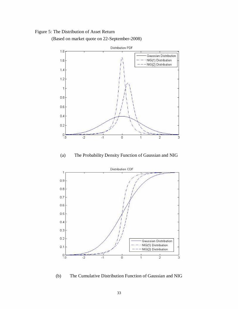
Figure 5: The Distribution of Asset Return
(Based on market quote on 22-September-2008)
(a) The Probability Density Function of Gaussian and NIG
(b) The Cumulative Distribution Function of Gaussian and NIG
34
(c) The Probability Density Function of NIG (1)
(d) The Cumulative Distribution Function of NIG (1)
35
(e) The Probability Density Function of NIG (2)
(f) The Cumulative Distribution Function of NIG (2)
36
Appendix B:
Table 3.5: The time series data of Default probability
(Implied by the market quote on 22-September-2008 and 20-March-2009)
t 22-Sep-08 20-Mar-09
0.25 0.0065 0.0112
0.5 0.0130 0.0223
0.75 0.0194 0.0333
1 0.0257 0.0442
1.25 0.0321 0.0549
1.5 0.0384 0.0655
1.75 0.0446 0.0760
2 0.0508 0.0864
2.25 0.0570 0.0966
2.5 0.0631 0.1068
2.75 0.0692 0.1168
3 0.0753 0.1267
3.25 0.0813 0.1365
3.5 0.0872 0.1462
3.75 0.0932 0.1558
4 0.0991 0.1653
4.25 0.1049 0.1747
4.5 0.1107 0.1839
4.75 0.1165 0.1931
5 0.1223 0.2021
37
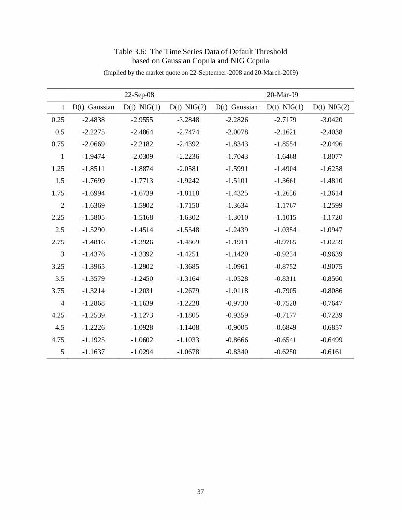
Table 3.6: The Time Series Data of Default Threshold based on Gaussian Copula and NIG Copula
(Implied by the market quote on 22-September-2008 and 20-March-2009)
22-Sep-08 20-Mar-09
t D(t)_Gaussian D(t)_NIG(1) D(t)_NIG(2) D(t)_Gaussian D(t)_NIG(1) D(t)_NIG(2)
0.25 -2.4838 -2.9555 -3.2848 -2.2826 -2.7179 -3.0420
0.5 -2.2275 -2.4864 -2.7474 -2.0078 -2.1621 -2.4038
0.75 -2.0669 -2.2182 -2.4392 -1.8343 -1.8554 -2.0496
1 -1.9474 -2.0309 -2.2236 -1.7043 -1.6468 -1.8077
1.25 -1.8511 -1.8874 -2.0581 -1.5991 -1.4904 -1.6258
1.5 -1.7699 -1.7713 -1.9242 -1.5101 -1.3661 -1.4810
1.75 -1.6994 -1.6739 -1.8118 -1.4325 -1.2636 -1.3614
2 -1.6369 -1.5902 -1.7150 -1.3634 -1.1767 -1.2599
2.25 -1.5805 -1.5168 -1.6302 -1.3010 -1.1015 -1.1720
2.5 -1.5290 -1.4514 -1.5548 -1.2439 -1.0354 -1.0947
2.75 -1.4816 -1.3926 -1.4869 -1.1911 -0.9765 -1.0259
3 -1.4376 -1.3392 -1.4251 -1.1420 -0.9234 -0.9639
3.25 -1.3965 -1.2902 -1.3685 -1.0961 -0.8752 -0.9075
3.5 -1.3579 -1.2450 -1.3164 -1.0528 -0.8311 -0.8560
3.75 -1.3214 -1.2031 -1.2679 -1.0118 -0.7905 -0.8086
4 -1.2868 -1.1639 -1.2228 -0.9730 -0.7528 -0.7647
4.25 -1.2539 -1.1273 -1.1805 -0.9359 -0.7177 -0.7239
4.5 -1.2226 -1.0928 -1.1408 -0.9005 -0.6849 -0.6857
4.75 -1.1925 -1.0602 -1.1033 -0.8666 -0.6541 -0.6499
5 -1.1637 -1.0294 -1.0678 -0.8340 -0.6250 -0.6161
38
Table 3.7: The Time Series Data of Expected Loss on Equity Tranche based on Gaussian Copula and NIG Copula
(Implied by the market quote on 22-September-2008 and 20-March-2009)
22-Sep-08 20-Mar-09
t EL(t)_Gaussian EL(t)_NIG(1) EL(t)_NIG(2) EL(t)_Gaussian EL(t)_NIG(1) EL(t)_NIG(2)
0.25 0.1294 0.1126 0.1123 0.2017 0.1537 0.1559
0.5 0.2524 0.2197 0.2235 0.3556 0.2944 0.3026
0.75 0.3639 0.3221 0.3288 0.4743 0.4225 0.4313
1 0.4621 0.4195 0.4268 0.5675 0.5370 0.5401
1.25 0.5468 0.5110 0.5167 0.6416 0.6359 0.6301
1.5 0.6190 0.5961 0.5967 0.7012 0.7177 0.7030
1.75 0.6802 0.6731 0.6674 0.7496 0.7813 0.7610
2 0.7316 0.7405 0.7283 0.7892 0.8281 0.8066
2.25 0.7749 0.7968 0.7796 0.8218 0.8613 0.8422
2.5 0.8111 0.8411 0.8220 0.8488 0.8849 0.8699
2.75 0.8414 0.8742 0.8564 0.8713 0.9021 0.8917
3 0.8668 0.8981 0.8840 0.8901 0.9148 0.9088
3.25 0.8880 0.9155 0.9059 0.9059 0.9246 0.9224
3.5 0.9058 0.9284 0.9232 0.9192 0.9323 0.9333
3.75 0.9206 0.9381 0.9369 0.9305 0.9385 0.9421
4 0.9331 0.9457 0.9477 0.9401 0.9436 0.9493
4.25 0.9436 0.9517 0.9563 0.9482 0.9479 0.9553
4.5 0.9523 0.9566 0.9632 0.9552 0.9515 0.9603
4.75 0.9597 0.9607 0.9687 0.9611 0.9546 0.9645
5 0.9659 0.9640 0.9732 0.9662 0.9573 0.9680
39
Appendix C: Matlab Code
(I) Gaussian Copula
1) EL_NormSDist.m -------------------------------------------------------------------------------- function EL_bivn=EL_NormSDist(K1,K2,R,C,a) % This function is developed to measure the expected loss of synthetic CDO % using LHP approach, which is based on one factor Gaussian copula model of % correlated defaults. % Author: Shirley Xin, Arvin Wang % Segal Graduate School of Business, Simon Fraser University % Date: July 18, 2010 X1=-norminv(K1/(1-R),0,1); X2=-norminv(K2/(1-R),0,1); X3=C; BiVar1=[X1;X3]; BiVar2=[X2;X3]; Mu=[0;0]; Sigma=[1 -sqrt(1-a^2);-sqrt(1-a^2) 1]; Phi1=mvncdf(BiVar1,Mu,Sigma); Phi2=mvncdf(BiVar2,Mu,Sigma); EL_bivn=(Phi1-Phi2)/((K2/(1-R))-(K1/(1-R))); end 2) Spread_Gaussian.m -------------------------------------------------------------------------------- clc clear all format long % This Script is developed to calculate the spreadpayment of synthetic CDO % tranches, based on one factor Gaussian Copula % Author: Shirley Xin, Arvin Wang % Segal Graduate School of Business, Simon Fraser University % Date: July 18, 2010 load CDXSpreadAvg.mat
40
% Set parameters K1=0; K2=0.03; R=0.4; Mat=5; a=sqrt(0.219201); rf=0.01670135; dt=0.25; % Calculate the discount factor DiscFact=ones(21,1); for i=1:1:Mat*4 DiscFact(i+1)=exp(-rf*i*0.25); end % Calculate the expected loss of the tranche EL=zeros(21,1); for i=1:1:Mat*4 EL(i+1)=EL_NormSDist(K1,K2,R,C_gaussian_d2(i),a); end % Protection Leg ProtectLeg=sum(diff(EL).*DiscFact(2:end)); % Premium Leg PremiumLeg=sum((1-EL(2:end)).*DiscFact(2:end)*dt); % Spread payment SpreadPayment=ProtectLeg/PremiumLeg
41
(II) Matlab Code for NIG Copula
*The Matlab toolbox of NIG distribution is available at Matlab Center File Exchange
1) intfunc.m -------------------------------------------------------------------------------- function y=intfunc(x,K1,R,C,a,alpha,beta,df) % Function developed in order to calculate the Expected Loss % y=intfunc(x,K1,R,C,a) % x = Unknown parameter % K1 = Attachment point of the tranche % R = Recovery % C = default threshold % a = sqrt(rho), where rho is the pairwise correlation of default % % Author: Shirley Xin, Arvin Wang % Segal Graduate School of Business, Simon Fraser University % Date: July 21, 2010 s=sqrt(1-a^2)/a; gamma=sqrt(alpha^2-beta^2); mu=beta*gamma^2/alpha^2; delta=gamma^3/alpha^2; temp1=nigcdf(x,s*alpha,s*beta,-s*mu,s*delta)-(K1/(1-R)); temp2=nigpdf((C-sqrt(1-a^2)*x)/a,df*alpha,df*beta,-df*mu,df*delta)*(sqrt(1-a^2)/a); y=temp1.*temp2; end 2) Spread_NIG.m -------------------------------------------------------------------------------- clc clear all format long % This Script is developed to calculate the spreadpayment of synthetic CDO % tranches, based on one factor NIG Copula % Author: Shirley Xin, Arvin Wang % Segal Graduate School of Business, Simon Fraser University % Date: July 20, 2010 % NIG toolbox developed by Kalemanova et al is available at Matlab Center

42
% File Exchange. load CDXSpreadAvg.mat % Set parameter values K1=1.000000000000000e-074; % attachment point of the tranche K2=0.03; % detachment point of the tranche R=0.4; % recovery rate Mat=5; % time to maturity a=sqrt(0.394263); % a=sqrt(rho), where rho is default correlation rf=0.01670135; % 5yr government zero rate dt=0.25; alpha=0.6020; % tail heavyness beta=-0.1605; % asymmetry parameter df=2; % NIG(df) gamma=sqrt(alpha^2-beta^2); s=sqrt(1-a^2)/a; mu=beta*gamma^2/alpha^2; delta=gamma^3/alpha^2; % Calculate the discount factor & Default threshold DiscFact=ones(21,1); C_NIG=zeros(20,1); for i=1:1:Mat*4 DiscFact(i+1)=exp(-rf*i*0.25); C_NIG(i)=niginv(DefProb_d2(i),alpha/a,beta/a,-(1/a)*mu,(1/a)*delta); end % Determine the expected loss EL(t) lowerbound=niginv(K1/(1-R),s*alpha,s*beta,-s*mu,s*delta); upperbound=niginv(K2/(1-R),s*alpha,s*beta,-s*mu,s*delta); FtK2=zeros(20,1); intFtK1=zeros(20,1); EL=zeros(21,1); for i=1:1:Mat*4 FtK2(i)=1-nigcdf((C_NIG(i)-sqrt(1-a^2)*upperbound)/a,df*alpha,df*beta,-df*mu,df*delta); intFtK1(i)=quad(@(x)intfunc(x,K1,R,C_NIG(i),a,alpha,beta,df),lowerbound,upperbound); EL(i+1)=((1-R)/(K2-K1))*intFtK1(i)+(1-FtK2(i)); end % Protection Leg ProtectLeg=sum(diff(EL).*DiscFact(2:end)); % Premium Leg PremiumLeg=sum((1-EL(2:end)).*DiscFact(2:end)*dt); % Spread payment SpreadPayment=ProtectLeg/PremiumLeg
43
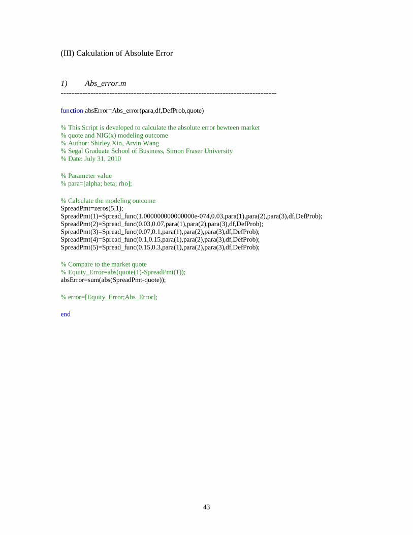
(III) Calculation of Absolute Error
1) Abs_error.m -------------------------------------------------------------------------------- function absError=Abs_error(para,df,DefProb,quote) % This Script is developed to calculate the absolute error bewteen market % quote and NIG(x) modeling outcome % Author: Shirley Xin, Arvin Wang % Segal Graduate School of Business, Simon Fraser University % Date: July 31, 2010 % Parameter value % para=[alpha; beta; rho]; % Calculate the modeling outcome SpreadPmt=zeros(5,1); SpreadPmt(1)=Spread_func(1.000000000000000e-074,0.03,para(1),para(2),para(3),df,DefProb); SpreadPmt(2)=Spread_func(0.03,0.07,para(1),para(2),para(3),df,DefProb); SpreadPmt(3)=Spread_func(0.07,0.1,para(1),para(2),para(3),df,DefProb); SpreadPmt(4)=Spread_func(0.1,0.15,para(1),para(2),para(3),df,DefProb); SpreadPmt(5)=Spread_func(0.15,0.3,para(1),para(2),para(3),df,DefProb); % Compare to the market quote % Equity_Error=abs(quote(1)-SpreadPmt(1)); absError=sum(abs(SpreadPmt-quote)); % error=[Equity_Error;Abs_Error]; end
44
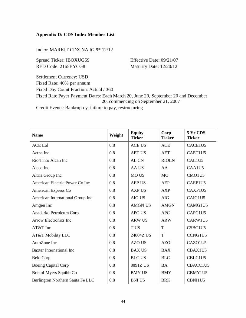
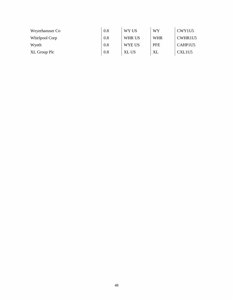
Appendix D: CDS Index Member List
Index: MARKIT CDX.NA.IG.9* 12/12
Spread Ticker: IBOXUG59
RED Code: 2165BYCG8
Effective Date: 09/21/07
Maturity Date: 12/20/12
Settlement Currency: USD
Fixed Rate: 40% per annum
Fixed Day Count Fraction: Actual / 360
Fixed Rate Payer Payment Dates: Each March 20, June 20, September 20 and December 20, commencing on September 21, 2007
Credit Events: Bankruptcy, failure to pay, restructuring
Name Weight Equity Ticker
Corp Ticker
5 Yr CDS Ticker
ACE Ltd 0.8 ACE US ACE CACE1U5
Aetna Inc 0.8 AET US AET CAET1U5
Rio Tinto Alcan Inc 0.8 AL CN RIOLN CAL1U5
Alcoa Inc 0.8 AA US AA CAA1U5
Altria Group Inc 0.8 MO US MO CMO1U5
American Electric Power Co Inc 0.8 AEP US AEP CAEP1U5
American Express Co 0.8 AXP US AXP CAXP1U5
American International Group Inc 0.8 AIG US AIG CAIG1U5
Amgen Inc 0.8 AMGN US AMGN CAMG1U5
Anadarko Petroleum Corp 0.8 APC US APC CAPC1U5
Arrow Electronics Inc 0.8 ARW US ARW CARW1U5
AT&T Inc 0.8 T US T CSBC1U5
AT&T Mobility LLC 0.8 24004Z US T CCNG1U5
AutoZone Inc 0.8 AZO US AZO CAZO1U5
Baxter International Inc 0.8 BAX US BAX CBAX1U5
Belo Corp 0.8 BLC US BLC CBLC1U5
Boeing Capital Corp 0.8 8891Z US BA CBACC1U5
Bristol-Myers Squibb Co 0.8 BMY US BMY CBMY1U5
Burlington Northern Santa Fe LLC 0.8 BNI US BRK CBNI1U5
45
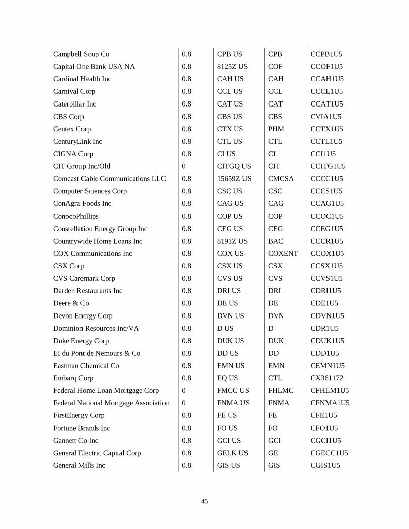
Campbell Soup Co 0.8 CPB US CPB CCPB1U5
Capital One Bank USA NA 0.8 8125Z US COF CCOF1U5
Cardinal Health Inc 0.8 CAH US CAH CCAH1U5
Carnival Corp 0.8 CCL US CCL CCCL1U5
Caterpillar Inc 0.8 CAT US CAT CCAT1U5
CBS Corp 0.8 CBS US CBS CVIA1U5
Centex Corp 0.8 CTX US PHM CCTX1U5
CenturyLink Inc 0.8 CTL US CTL CCTL1U5
CIGNA Corp 0.8 CI US CI CCI1U5
CIT Group Inc/Old 0 CITGQ US CIT CCITG1U5
Comcast Cable Communications LLC 0.8 15659Z US CMCSA CCCC1U5
Computer Sciences Corp 0.8 CSC US CSC CCCS1U5
ConAgra Foods Inc 0.8 CAG US CAG CCAG1U5
ConocoPhillips 0.8 COP US COP CCOC1U5
Constellation Energy Group Inc 0.8 CEG US CEG CCEG1U5
Countrywide Home Loans Inc 0.8 8191Z US BAC CCCR1U5
COX Communications Inc 0.8 COX US COXENT CCOX1U5
CSX Corp 0.8 CSX US CSX CCSX1U5
CVS Caremark Corp 0.8 CVS US CVS CCVS1U5
Darden Restaurants Inc 0.8 DRI US DRI CDRI1U5
Deere & Co 0.8 DE US DE CDE1U5
Devon Energy Corp 0.8 DVN US DVN CDVN1U5
Dominion Resources Inc/VA 0.8 D US D CDR1U5
Duke Energy Corp 0.8 DUK US DUK CDUK1U5
EI du Pont de Nemours & Co 0.8 DD US DD CDD1U5
Eastman Chemical Co 0.8 EMN US EMN CEMN1U5
Embarq Corp 0.8 EQ US CTL CX361172
Federal Home Loan Mortgage Corp 0 FMCC US FHLMC CFHLM1U5
Federal National Mortgage Association 0 FNMA US FNMA CFNMA1U5
FirstEnergy Corp 0.8 FE US FE CFE1U5
Fortune Brands Inc 0.8 FO US FO CFO1U5
Gannett Co Inc 0.8 GCI US GCI CGCI1U5
General Electric Capital Corp 0.8 GELK US GE CGECC1U5
General Mills Inc 0.8 GIS US GIS CGIS1U5
46
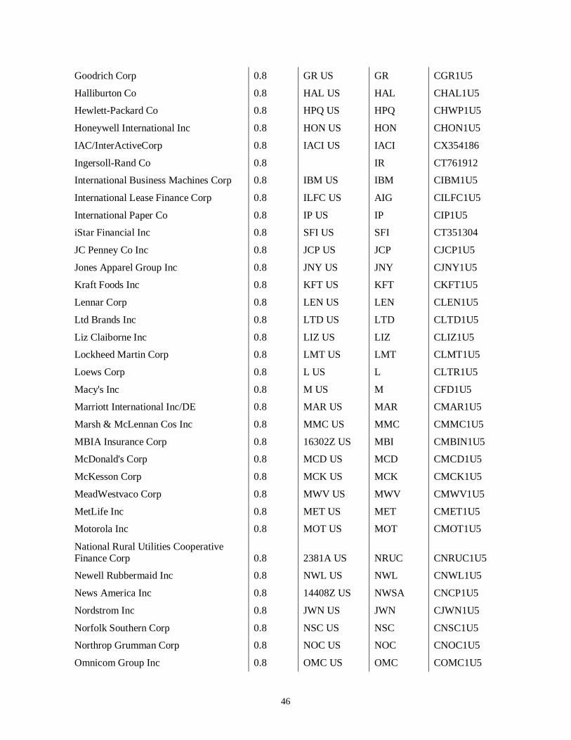
Goodrich Corp 0.8 GR US GR CGR1U5
Halliburton Co 0.8 HAL US HAL CHAL1U5
Hewlett-Packard Co 0.8 HPQ US HPQ CHWP1U5
Honeywell International Inc 0.8 HON US HON CHON1U5
IAC/InterActiveCorp 0.8 IACI US IACI CX354186
Ingersoll-Rand Co 0.8 IR CT761912
International Business Machines Corp 0.8 IBM US IBM CIBM1U5
International Lease Finance Corp 0.8 ILFC US AIG CILFC1U5
International Paper Co 0.8 IP US IP CIP1U5
iStar Financial Inc 0.8 SFI US SFI CT351304
JC Penney Co Inc 0.8 JCP US JCP CJCP1U5
Jones Apparel Group Inc 0.8 JNY US JNY CJNY1U5
Kraft Foods Inc 0.8 KFT US KFT CKFT1U5
Lennar Corp 0.8 LEN US LEN CLEN1U5
Ltd Brands Inc 0.8 LTD US LTD CLTD1U5
Liz Claiborne Inc 0.8 LIZ US LIZ CLIZ1U5
Lockheed Martin Corp 0.8 LMT US LMT CLMT1U5
Loews Corp 0.8 L US L CLTR1U5
Macy's Inc 0.8 M US M CFD1U5
Marriott International Inc/DE 0.8 MAR US MAR CMAR1U5
Marsh & McLennan Cos Inc 0.8 MMC US MMC CMMC1U5
MBIA Insurance Corp 0.8 16302Z US MBI CMBIN1U5
McDonald's Corp 0.8 MCD US MCD CMCD1U5
McKesson Corp 0.8 MCK US MCK CMCK1U5
MeadWestvaco Corp 0.8 MWV US MWV CMWV1U5
MetLife Inc 0.8 MET US MET CMET1U5
Motorola Inc 0.8 MOT US MOT CMOT1U5
National Rural Utilities Cooperative Finance Corp 0.8 2381A US NRUC CNRUC1U5
Newell Rubbermaid Inc 0.8 NWL US NWL CNWL1U5
News America Inc 0.8 14408Z US NWSA CNCP1U5
Nordstrom Inc 0.8 JWN US JWN CJWN1U5
Norfolk Southern Corp 0.8 NSC US NSC CNSC1U5
Northrop Grumman Corp 0.8 NOC US NOC CNOC1U5
Omnicom Group Inc 0.8 OMC US OMC COMC1U5

47
Progress Energy Inc 0.8 PGN US PGN CPGN1U5
Pulte Group Inc 0.8 PHM US PHM CPHM1U5
Quest Diagnostics Inc/DE 0.8 DGX US DGX CDGX1U5
RR Donnelley & Sons Co 0.8 RRD US RRD CX359760
Radian Group Inc 0.8 RDN US RDN CRDN1U5
Raytheon Co 0.8 RTN US RTN CRTN1U5
Rohm and Haas Co 0.8 ROH US DOW CROH1U5
Safeway Inc 0.8 SWY US SWY CSWY1U5
Sara Lee Corp 0.8 SLE US SLE CSLE1U5
Sempra Energy 0.8 SRE US SRE CSRE1U5
Simon Property Group LP 0.8 12968Z US SPG CSPG1U5
Southwest Airlines Co 0.8 LUV US LUV CLUV1U5
Sprint Nextel Corp 0.8 S US S CT357422
Starwood Hotels & Resorts Worldwide Inc 0.8 HOT US HOT CHOT1U5
Target Corp 0.8 TGT US TGT CTGT1U5
Textron Financial Corp 0.8 3339Z US TXT CTXTF1U5
Allstate Corp/The 0.8 ALL US ALL CALL1U5
Chubb Corp 0.8 CB US CB CCB1U5
Dow Chemical Co/The 0.8 DOW US DOW CDOW1U5
Hartford Financial Services Group Inc 0.8 HIG US HIG CHIG1U5
Home Depot Inc 0.8 HD US HD CHD1U5
Kroger Co/The 0.8 KR US KR CKR1U5
Sherwin-Williams Co/The 0.8 SHW US SHW CSHW1U5
Walt Disney Co/The 0.8 DIS US DIS CDIS1U5
Time Warner Inc 0.8 TWX US TWX CAOL1U5
Toll Brothers Inc 0.8 TOL US TOL CTOL1U5
Transocean Inc 0.8 3196976Z US RIG CRIG1U5
Union Pacific Corp 0.8 UNP US UNP CUNP1U5
Universal Health Services Inc 0.8 UHS US UHS CT357677
Valero Energy Corp 0.8 VLO US VLO CVLO1U5
Verizon Communications Inc 0.8 VZ US VZ CVZGF1U5
Wal-Mart Stores Inc 0.8 WMT US WMT CWMT1U5
Washington Mutual Inc 0 WAMUQ US WM CWM1U5
Wells Fargo & Co 0.8 WFC US WFC CWFC1U5
48
Weyerhaeuser Co 0.8 WY US WY CWY1U5
Whirlpool Corp 0.8 WHR US WHR CWHR1U5
Wyeth 0.8 WYE US PFE CAHP1U5
XL Group Plc 0.8 XL US XL CXL1U5


![The Matrix Generalized Inverse Gaussian …baner029/papers/16/CMCPMF.pdfMatrix Generalized Inverse Gaussian (MGIG) distributions [3,10] are a family of distributions over the space](https://img.pdfslide.net/doc/110x75/5f04904f7e708231d40e9764/the-matrix-generalized-inverse-gaussian-baner029papers16-matrix-generalized-inverse.jpg)