Embed Size (px)
Citation preview

Validation of Spent Fuel Dose Rate Calculations
Using NDA Measurement Campaign Data
ANL-20/54
Nuclear Science and Engineering Division

About Argonne National Laboratory
Argonne is a U.S. Department of Energy laboratory managed by UChicago Argonne, LLC
under contract DE-AC02-06CH11357. The Laboratory’s main facility is outside Chicago, at
9700 South Cass Avenue, Argonne, Illinois 60439. For information about Argonne
and its pioneering science and technology programs, see www.anl.gov.
DOCUMENT AVAILABILITY
Online Access: U.S. Department of Energy (DOE) reports produced after 1991 and a
growing number of pre-1991 documents are available free at OSTI.GOV
(http://www.osti.gov/), a service of the US Dept. of Energy’s Office of Scientific and
Technical Information.
Reports not in digital format may be purchased by the public from the
National Technical Information Service (NTIS):
U.S. Department of Commerce
National Technical Information Service
5301 Shawnee Rd
Alexandria, VA 22312
www.ntis.gov
Phone: (800) 553-NTIS (6847) or (703) 605-6000
Fax: (703) 605-6900
Email: [email protected]
Reports not in digital format are available to DOE and DOE contractors from the
Office of Scientific and Technical Information (OSTI):
U.S. Department of Energy
Office of Scientific and Technical Information
P.O. Box 62
Oak Ridge, TN 37831-0062
www.osti.gov
Phone: (865) 576-8401
Fax: (865) 576-5728
Email: [email protected]
Disclaimer
This report was prepared as an account of work sponsored by an agency of the United States Government. Neither the United States
Government nor any agency thereof, nor UChicago Argonne, LLC, nor any of their employees or officers, makes any warranty, express or
implied, or assumes any legal liability or responsibility for the accuracy, completeness, or usefulness of any information, apparatus,
product, or process disclosed, or represents that its use would not infringe privately owned rights. Reference herein to any specific
commercial product, process, or service by trade name, trademark, manufacturer, or otherwise, does not necessarily constitute or imply its
endorsement, recommendation, or favoring by the United States Government or any agency thereof. The views and opinions of document
authors expressed herein do not necessarily state or reflect those of the United States Government or any agency thereof, Argonne
National Laboratory, or UChicago Argonne, LLC.

ANL-20/54
Validation of Spent Fuel Dose Rate Calculations Using NDA
Measurement Campaign Data
prepared by
Yan Cao, Matthew Boyd, and Bo Feng
Nuclear Science and Engineering Division, Argonne National Laboratory
09/02/2020

Validation of Spent Fuel Dose Rate Calculations Using NDA Measurement Campaign Data
Yan Cao, Matthew Boyd, and Bo Feng
Argonne National Laboratory
Updated: May 29, 2020
1. Introduction
The predicted radiation gamma dose rate is a key parameter to determine if a spent nuclear fuel
assembly is self-protected from misuse as well as an indicator for worker/inspector safety. Recent
studies [1, 2, 3] showed that using state-of-the-art techniques for dose rate calculations, including
the one adopted for this study, the numerical calculations of the gamma dose rates are three times
lower than those from the most commonly-cited reference values for spent LWR fuel [4] used by
domestic and international agencies. With only a few publically available experimental data points
worldwide for this type of benchmark study, the gamma flux measurements from the Spent Fuel
Non Destructive Assay (NDA) measurement campaign can be used to help validate the physics
approach used in calculating gamma dose rates [5]. Specifically, this data would validate the
gamma flux calculation from spent fuel, which is a key component of these multi-physics
techniques for dose rate assessments; dose rate measurements were not part of the NDA campaign.
These data are primarily the passive gamma measurements of the spent nuclear fuel assemblies
from the Swedish Nuclear Fuel and Waste Management Company (SKB) [5].
Figure 1 Schematic of experiment setup of the passive gamma measurements [6]

The NDA data includes passive gamma fluxes that were measured for 25 PWR and 25 BWR fuel
assemblies, labeled only as “PWR1, PWR2, etc.” to remove identifying information, using the
high-purity germanium detectors or lanthanum bromide scintillation detectors. Figure 1 shows a
schematic of the experimental setup of these measurements [6]. Each fuel assembly was placed in
the pool at Sweden’s Central Interim Storage Facility (Clab) with one of its corners facing a steel
collimator which was built into the pool wall. The fuel assembly was rotated with four corners
each facing the collimator to allow four static measurements of the gamma fluxes. The fuel
assembly was also moved up and down to allow integral scans along the vertical direction for the
gamma fluxes at each of the four angles. Therefore, each fuel assembly has a total of 8 gamma
spectra available for comparison [7].
2. Simplified Bare Assembly (Item) Models
The NDA data was provided to ANL from LANL in the form of measured passive gamma counts
at several energy peaks in Excel spreadsheets and MCNP models of all 50 assemblies or items.
These MCNP models contain detailed isotopic compositions of the fuels, source terms, cladding
and structural information, and assembly geometry. Note that the experimental environment (pool,
detectors, collimator, etc.) was not included in these MCNP models. Nevertheless, in terms of the
fuel material description, the models were deemed to contain too much compositional detail for
the purposes of dose rate calculations, which would significantly slow down the calculation
process. This section describes how these MCNP models of bare assemblies were simplified by
ANL for the sole purpose of speeding up the calculations while not losing too much accuracy.
Shortly after the measurements were obtained from the NDA campaign, significant modeling work
was already performed by various laboratories to model the irradiation and decay of those fuel
assemblies [8]. At ORNL, the ORIGAMI code was used in the fuel burnup and fuel decay
simulations to provide the compositions in the MCNP models received by ANL. ORIGAMI was
used to generate nuclide compositions for each axial node of each fuel pin in a fuel assembly. For
the SKB PWR fuel assemblies, each fuel pin was divided into nine axial nodes. With more than
200 fuel pins in each fuel assembly, the total number of fuel zones for one assembly is more than
1800 in one fuel assembly model. ANL received three MCNP input decks for each fuel assembly.
The “Upper”, “Mid” and “Lower” input decks describe the upper, middle, and lower axial parts of
the fuel assembly, respectively, with vacuum boundary conditions applied outside the assembly.
To model the gamma transport and simulate the gamma spectra, ANL first combined the three
MCNP input decks into one single MCNP model so that the numerical calculations can correctly
count the gamma contributions from all the axial zones of the fuel assembly. The original fine
discretization of different fuel burnup zones inside the fuel assembly led to a significantly large
number of fuel materials and source terms which are not critical for gamma transport simulations
and are almost impossible to handle in a single MCNP transport simulation.
To simplify the MCNP models, for each axial layer of the fuel assembly, the fuel pins that have
similar fuel burnups and gamma sources in the ORIGAMI calculations were grouped together as
one pin type. The nuclide compositions for those similar fuel zones were then homogenized to one
fuel composition. The discrete gamma energy lines for those similar fuel pins were homogenized
as well into one gamma source spectrum representing an average of 6 pins. Figure 2 compares the
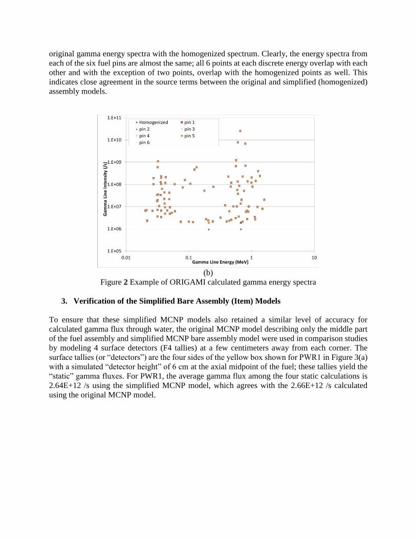
original gamma energy spectra with the homogenized spectrum. Clearly, the energy spectra from
each of the six fuel pins are almost the same; all 6 points at each discrete energy overlap with each
other and with the exception of two points, overlap with the homogenized points as well. This
indicates close agreement in the source terms between the original and simplified (homogenized)
assembly models.
(b)
Figure 2 Example of ORIGAMI calculated gamma energy spectra
3. Verification of the Simplified Bare Assembly (Item) Models
To ensure that these simplified MCNP models also retained a similar level of accuracy for
calculated gamma flux through water, the original MCNP model describing only the middle part
of the fuel assembly and simplified MCNP bare assembly model were used in comparison studies
by modeling 4 surface detectors (F4 tallies) at a few centimeters away from each corner. The
surface tallies (or “detectors”) are the four sides of the yellow box shown for PWR1 in Figure 3(a)
with a simulated “detector height” of 6 cm at the axial midpoint of the fuel; these tallies yield the
“static” gamma fluxes. For PWR1, the average gamma flux among the four static calculations is
2.64E+12 /s using the simplified MCNP model, which agrees with the 2.66E+12 /s calculated
using the original MCNP model.

(a)
(b)
Figure 3 (a) MCNP model with the surface tallies facing four corners of the fuel assemblies. (b)
Tallied gamma flux dispersion using both the simplified and original MCNP models for PWR1
In addition, Figure 3(b) shows the gamma flux dispersion (relative flux at each corner compared
to the average) using both models. This dispersion along with the average static gamma fluxes
indicate that the simplified MCNP model retains excellent agreement with the original MCNP
models in terms of gamma transport through water.
4. Validation of the Simplified Bare Assembly (Item) Models
Following the same procedure, simplified MCNP models were developed for all 25 PWR fuel
assemblies with the goal of comparing the calculated gamma fluxes from these models to those
from the measured data. However, since these MCNP models are bare spheres and the measured
data were obtained with a full experimental environment, it was only possible to compare
0.60
0.70
0.80
0.90
1.00
1.10
1.20
0 50 100 150 200 250 300 350
Gam
ma
Co
un
ts (
Gam
ma
Flu
x Ta
llie
s) t
o I
ts A
vera
ge
Detector Facing Angle to the Fuel Assembly (Degree)
Simplified MCNP6 model
Original MCNP6 model

normalized gamma flux values rather than absolute values. Available data provided to ANL
consisted of count rates for 13 peaks from 6 isotopes: 1 from Cs-137, 5 from Cs-134, 4 from Eu-
154, and an additional 1 line each from K-40, Ce-144, and Rh-106. For this validation exercise,
the key gamma peak for LWR dose rate calculations (662 keV from Cs-137 decay) was selected
for comparison. Both the 4-side averaged static gamma measurements and the 4-side averaged
scanned gamma measurements were also normalized and compared to the calculated normalized
values from MCNP. In the MCNP model, the scanned flux is simply assumed to be the flux through
a surface tally along the entire axial length of the fuel assembly rather than the flux within the 6
cm “detector” for the static flux.
Figure 4 Average gamma counts (or flux) at 662 keV energy level for each PWR assembly
compared to those for PWR8 produced from measurements and MCNP simulations
Figure 4 shows the 4-side averaged static and scanned gamma fluxes for the 662 keV peak
calculated from MCNP and compared to those from the experiments. In order to produce this
figure to compare relative results, the calculated or measured flux from each of the 25 assemblies
was normalized to the calculated or measured flux from PWR8. Initially, PWR1’s values were
chosen as the normalization factors, but due to the large disagreements between calculated and
measured scanned fluxes in the first 7 assemblies, our best guess was that PWR8 serves as the
normalization assembly that allows the best agreement across all 25 assemblies.
With a few exceptions (PWR4, PWR5, and PWR7), the relative experimental static flux, calculated
static flux, and calculated scanned flux are in almost exact agreement in this figure. Those three
exceptions show slightly lower experimental static fluxes, assuming PWR8 has all the “correct”
values. The experimental scanned flux also shows excellent agreement for only about half of the
assemblies.

The reason for the differences shown for the calculated vs. experimental scanned flux results is
not clear. The MCNP model only modeled the bare fuel assembly with all the other structure
materials ignored. Based on our previous knowledge, the gamma fluxes due to the irradiation of
the structural materials can be significant contributions in some cases [5]. The scanned
experiments read contributions of gamma fluxes from the whole fuel assembly including spacers.
In addition, in the experiment, the scanned gamma fluxes were taken by moving the fuel
assemblies passing the collimator slit. The exact motion of the fuel assembly is unknown. All these
factors may lead to the scanned fluxes different from a simple integration of the gamma flux of
the whole fuel assembly we assumed in the MCNP model. Therefore, in the later analysis, only
those experimental data from static measurements are utilized in the analysis. Particularly, MCNP
simulations with the full environment are limited to PWRs 1-2 for validation purposes.
5. Experimental Setup of Gamma Measurements and Corresponding MCNP Model
In the actual experimental setup for the passive gamma measurements, as previously shown in
Figure 1, the distance from the assembly center to the pool wall was 50 cm [9, 10]. Figure 5 shows
an MCNP modelof the horizontal cross section of the steel collimator consisting of two steel half
cylinders 120 cm long and 27 cm in diameter built into the pool wall at ~10 m below the surface
level of the water [11, 12, 13].
The vertical width of the collimator slit was set to 5 mm [11, 13]. The horizontal width of the slit
is sufficient to view the entire quadratic of the fuel assembly at the fuel end but narrows to a 5 cm
opening at the detector end [10]. The distance from the center of the assembly to the end of the
collimator was 2.46 m. The central axis of the detector was positioned 3 mm below the vertical
plane of the detector to optimize the signal-to-background ratio [11].
The Clab fuel pool is steel lined, but no information could be found on the liner thickness [14]. A
value of 7 mm was assumed for this work based on the liner thickness at the Barsebeck-2 BWR
plant in Sweden [15]. Several additional attenuators were positioned after the collimator, and their
composition and thickness depends on the specific measurement campaign [11]. In the work
performed in 2019 fiscal year, the 3.2 mm lead and 1mm copper from the fourth measurement
campaign were assumed. After careful consideration, we believe the measurements for all PWRs
were done in the third measurement campaign, and thus the attenuators in the models were updated
to be 8 mm of lead, 21 mm of stainless steel, 3 mm of aluminum, and 1 mm of copper.

Figure 5 MCNP model horizontal cross-section at collimator slit location.
In the MCNP model, the water pool was represented as a 50 cm square block of water. A 7 mm
steel liner separates the water from a 120 cm thick concrete wall and empty cavity for the
collimator. The steel collimator begins 126 cm from the center of the assembly. The attenuators
are located after the collimator. The experimental data provided to ANL was measured using the
high-purity germanium (HPGe) detectors. For the MCNP models, an HPGe detector endcap and
crystal was modeled based on typical values, obtained from the manufacturer [11]. The Ge crystal
is 6.27 cm in diameter and 6.05 cm length [16]. For the model used in the experimental work, a
Canberra GX4518 (45% efficiency) was used based on reported specifications.
6. Validation of Detector Model
To first test the accuracy of the model for the HPGe, a simple MCNP simulation was conducted
to replicate the standard relative efficiency test of the reference 3x3 NaI(Tl) scintillator detector
[11]. In the model, a Co-60 source was placed 25 cm from the detector endcap face. The MCNP
F8 ‘Pulse Height’ tally was used to simulate a detector response during the photon transport and
will be used in the MCNP models discussed in the next section, which include the detector and
experimental setup. The F8 tally records the energy or charge deposited by each source particle
and its secondary particles, and the number of pulses depositing energy in a particle energy bin are
tallied. By providing an appropriate energy binning, a direct comparison can be obtained between
the simulated pulse height in MCNP and the experimental count rate for a given peak, such as the
ones provided for the 3x3 NaI(T1).
The resulting spectra can be seen in Figure 7 with the full spectra on the left and a zoomed in view
of the Co-60 peaks on the right. The normalized tally results are plotted as a function of energy.
The two Co-60 peaks can clearly be seen along with other features such as the Compton edge and
continuum, the discontinuity is a plotting aberration. The tally statistical error was around 6% for
the 1.33 MeV peak. The area of the Co-60 1.33 MeV peak was then divided by the absolute
efficiency of a 3x3 NaI(T1), which is 1.2x10⁻³, to a obtain a relative efficiency of ~54%. The ~20%
difference between the nominal 45% [11] and obtained 54% indicates relatively good agreement
with the differences likely due to inaccuracies in the Ge dead layer thickness. The expected spectral
features are present in Figure 6 and the model appears to respond correctly, indicating that the
detectors were modeled with sufficient accuracy.
AttenuatorsFuel Assembly
Water Collimator
Concrete Wall
HPGe Detector

Figure 6 MCNP F8 tally results for modeled detector 1.33 MeV relative efficiency comparison
7. Validation of MCNP Models of Environment
The work discussed up to Section 4 and summarized in Figure 4 only involved MCNP bare
assembly models without the experimental environment. Therefore, only the relative gamma
fluxes were compare-able between the bare assembly models and the measured data, and they
largely showed excellent agreement. The results in this section focus on validating the MCNP
models of the assemblies within the full environment, so now the tallied detector count rates in
MCNP can be directly compared with the experimental data.
The amount of the shielding material from the water, collimator, and concrete wall will
significantly reduce the gammas fluxes compared to the bare assembly models. Therefore, weight-
windows were used to reduce the variances of the photon flux tallies in the detector tally zone.
Figure 7 shows the weight-window generated for the simulation of the PWR1 fuel assembly. The
MCNP weight window tallies showed significantly increasing of particle importance along its
trajectory to the detector. Given the large effort required to generate these weight windows, only
the results for the first two PWR fuel assemblies are presented here.
Figure 7 MCNP Generated Weight-Window (WWG) for detector tallies.
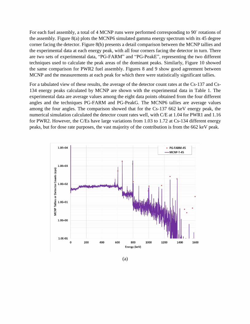
For each fuel assembly, a total of 4 MCNP runs were performed corresponding to 90⸰ rotations of
the assembly. Figure 8(a) plots the MCNP6 simulated gamma energy spectrum with its 45 degree
corner facing the detector. Figure 8(b) presents a detail comparison between the MCNP tallies and
the experimental data at each energy peak, with all four corners facing the detector in turn. There
are two sets of experimental data, “PG-FARM” and “PG-PeakE”, representing the two different
techniques used to calculate the peak areas of the dominant peaks. Similarly, Figure 10 showed
the same comparison for PWR2 fuel assembly. Figures 8 and 9 show good agreement between
MCNP and the measurements at each peak for which there were statistically significant tallies.
For a tabulated view of these results, the average of the detector count rates at the Cs-137 and Cs-
134 energy peaks calculated by MCNP are shown with the experimental data in Table 1. The
experimental data are average values among the eight data points obtained from the four different
angles and the techniques PG-FARM and PG-PeakG. The MCNP6 tallies are average values
among the four angles. The comparison showed that for the Cs-137 662 keV energy peak, the
numerical simulation calculated the detector count rates well, with C/E at 1.04 for PWR1 and 1.16
for PWR2. However, the C/Es have large variations from 1.03 to 1.72 at Cs-134 different energy
peaks, but for dose rate purposes, the vast majority of the contribution is from the 662 keV peak.
(a)

(b)
Figure 8 (a) MCNP6 tallied gamma energy spectrum from PWR1 fuel assembly by the HPGe
detector. (b) MCNP6 tallied detector counting rates from the PWR1 fuel assembly at each
gamma energy peak.
Figure 9 MCNP6 tallied detector counting rates for the SKB PWR2 fuel assembly at each energy
peak.

Table 1 MCNP calculated count rates at each peak for PWR1 and PWR2 fuel assemblies
compared with the NDA data.
Nuclide Cs-137 Cs-134
Energy Peak 662 keV 605 keV 796 keV 801 keV 1167
keV
1365
keV
PWR1
Exp 1817.5 508.1 1208.1 124.3 78.6 189.9
uncertainty 7.8 4.0 7.3 2.9 1.4 2.3
MCNP6 1901.2 857.2 1666.6 128.0 104.2 170.4
uncertainty 30.2 47.8 143.4 21.7 25.9 27.6
C/E 1.05 1.69 1.38 1.03 1.33 0.9
PWR2
Exp 1704.1 442.8 1151.1 105.2 66.8 162.0
uncertainty 7.7 3.4 7.0 2.7 1.2 1.9
MCNP6 1976.9 762.0 1445.0 151.4 69.7 212.4
uncertainty 79.9 32.1 141.0 33.8 17.3 20.2
C/E 1.16 1.72 1.26 1.44 1.04 1.31
8. Calculated Dose Rates
Assuming that additional effort would yield similar agreement in the 662 keV gamma flux results
for the remaining 23 PWR assemblies, then the modeling approach used in this study can be
considered validated for gamma flux calculations via the NDA measurements. This approach for
modeling the radiation transport is a key component of a larger multi-step approach for dose rate
calculations. Although the dose rates were not measured for these PWR assemblies, they were
nevertheless calculated in this study for future use and reference. This mostly involved using flux
dose rate conversion factors (namely, the 1991 ANS conversion factor [17]) that are energy-
dependent. Table 2 shows the results for each fuel assembly. Figure 10 plots the calculated gamma
dose rates according to its fuel burnup.

Figure 10: MCNP6 calculated gamma dose rates for the 25 SKB PWR fuel assemblies at the fuel
center plane 1 meter away from the assembly surface.
In the figure, the different color bars represent the different cooling time periods of each fuel
assembly after being discharged. Overall, the dose rates are higher for fuel assemblies with higher
burnup, as expected. The fuel assembly dose rates also decrease significantly after a few extra
years of cooling. To compare these results to those from the benchmark study [1], the results from
fuel assembly PWR22 were selected since its characteristics (fuel burnup of 31.7 GWd/tU and
decay time of 28 years) match closest to those from the reference example. PWR22’s gamma dose
rate of ~ 5.02 Sv/hr is entirely consistent with the results from that study.
Table 2 MCNP calculated gamma dose rates from the 25 PWR fuel assembly at the axial
midpoint of the active fuel assembly and about 1 meter away from the closest surface
Assembly IE BU CT Dose Rates
ID (wt U235%) (GWd/tU) (yrs) (Rem/hr)
PWR1 4.10 52.630 5.4 3436.03
PWR2 3.93 49.555 5.4 3060.32
PWR3 3.69 48.175 14.3 1188.85
PWR4 3.93 46.873 6.3 2439.56
PWR5 3.94 46.866 6.4 2306.99
PWR6 3.60 45.658 15.3 1056.55
PWR7 3.94 44.483 7.3 1924.01

PWR8 3.30 44.375 26.1 731.47
PWR9 3.71 45.846 7.2 2048.11
PWR10 3.70 43.474 16.3 941.66
PWR11 3.51 43.225 14.3 962.30
PWR12 3.30 42.969 26.1 744.97
PWR13 3.20 40.920 27.5 678.91
PWR14 3.51 40.745 17.3 826.20
PWR15 2.80 40.473 27.1 668.04
PWR16 3.60 40.410 18.3 795.87
PWR17 3.70 40.294 15.1 902.38
PWR18 3.52 39.756 19.3 730.88
PWR19 3.20 35.027 29.4 506.76
PWR20 3.10 34.032 28.3 526.65
PWR21 3.10 34.019 28.3 526.74
PWR22 2.80 31.165 28.2 502.11
PWR23 3.60 28.499 18.3 562.99
PWR24 2.10 23.151 19.3 383.96
PWR25 2.10 19.607 30.4 297.03
9. Summary
The MCNP photon transport simulation of the spent fuel assemblies and experimental facility
showed very promising agreement (5% to 16% error) of the calculated photon fluxes at the energy
peak of Cs-137 662 keV, which is the dominant radiation dose contributor in the spent LWR fuel
assemblies. The agreement at other gamma energy peaks, particularly for the Cs-134 energy peaks
is not as great as at the Cs-137 energy peak. The agreement ranges from a few percent to about
70% more in the MCNP tallied count rates. Due to the limited effort, MCNP simulations were
performed only to the first two PWR fuel assemblies. Future simulation work to involve more
spent fuel assemblies can provide more information to explain some of the differences or pinpoint
the source of discrepancies in the above analysis. In addition, in these simulations, the detector
model showed about 20% higher efficiency (54% vs. 45%) than that reported from the
manufacturer. Future simulations with improved detector models may also improve the simulation
results to the experimental data.
10. Acknowledgements
The authors acknowledge support of the Office of Nonproliferation and Arms Control, U. S.
Department of Energy’s National Nuclear Security Administration, and the Clab interim storage
facility in Sweden. The measurements were performed as part of Action Sheet 50 “Spent Fuel
NDA Research for Safeguarding Future Encapsulation/Repository Facilities.” Action Sheet 50 of
the Euratom-United States Department of Energy (DOE) agreement outlined the work in Sweden

under the Cooperation Agreement on Nuclear Material Safeguards and Security Research and
Development between the US Department of Energy, the European Atomic Energy Community,
and SKB in Sweden.
The authors also would like to thank Dr. Holly Trellue (LANL) for her help providing the relevant
information and guidance to complete our work.
References
[1] B. Feng, R.N. Hill, R. Girieud, R. Eschbach, “Comparison of Gamma Dose Rate
Calculations for PWR Spent Fuel Assemblies,” The Role of Reactor Physics Toward a
Sustainable Future PHYSOR 2014, The Westin Miyako, Kyoto, Japan, Sep 28 – Oct 3,
2014 (2014).
[2] Y. Cao and B. Feng, “Validation of Gamma Dose Rate Calculation Methodology using
the Morris and Turkey Point Measurements,” ANL-19/06 (2019).
[3] R. Eschbach, B. Feng, etc., “Verification of Dose Rate Calculations for PWR Spent Fuel
Assemblies,” Proceedings of GLOBAL 2017 International Nuclear Fuel Cycle
Conference, September 24-29, 2017 –Soeul (korea (2017).
[4] W.R. Lloyd, M.K. Sheaffer, and W.G. Sutcliffe, “Dose Rate Estimates from Irradiated
Light-Water-Reactor Fuel Assemblies in Air,” Lawrence Livermore National Laboratory,
Livermore, CA, UCRL-ID-115199 (1994)
[5] H. Trellue, D. Henzlova, A. LaFleur, J. Eigenbrodt, “Spent Fuel Nondestructive Assay
(NDA) Experiences and Successes,” LA-UR-18-25995 (2018).
[6] Vaccaro, S., Tobin, Stephen Joseph, Favalli, Andrea, Grogan, Brandon R., Jansson, Peter,
Liljenfeldt, Henrik, Mozin, Vladimir, Hu, Jianwei, Schwalbach, P., Sjoland, A., Trellue,
Holly Renee, and Vo, Duc Ta. Sun . "PWR and BWR spent fuel assembly gamma spectra
measurements". United States. doi:10.1016/j.nima.2016.07.032.
https://www.osti.gov/servlets/purl/1287045. https://www.osti.gov/biblio/1287045
[7] A. Favalli, D. Vo, B. Grogan, P. Jansson, H. Liljenfeldt, V. Mozin, P. Schwalbach, A.
Sjoland, S.J. Tobin, H. Trellue, S. Vaccaro, “Determining Initial Enrichment, Burnup,
and Cooling Time of Pressurized-Water-Reactor Spent Fuel Assemblies by Analyzing
Passive Gamma Spectra Measured at the Clab Interim-Fuel Storage Facility in Sweden,”
Nucl. Inst. Meth. Phys. Res. A, 820, 102-111 (2006).
[8] J. Hu, I. Gauld, “Spent Nuclear Fuel Modeling & Simulation and Measurements,” Spent
Fuel Data Meeting at LANL, 2019.
[9] C. Willman, “Applications of Gamma Ray Spectroscopy of Spent Nuclear Fuel for
Safeguards and Encapsulation.” Uppsala Univeritet, 2006.
[10] A. Hakansson and A. Backlin, “Non-destructive Assay of Spent BWR Fuel with High-
resolution Gamma-ray Spectroscopy,” p. 36, ISSN 1104-1374, 1995.

[11] S. Vaccaro et al., “PWR and BWR spent fuel assembly gamma spectra measurements,”
Nuclear Instruments and Methods in Physics Research Section A: Accelerators,
Spectrometers, Detectors and Associated Equipment, vol. 833, pp. 208–225, Oct. 2016.
[12] Ludewigt, Bernhard, Mozin, Vladimir, Campbell, Luke, Favalli, Andrea, Alan W. Hunt,
Reedy, Edward T.E., and Seipel, Heather. Mon . "Delayed Gamma-Ray Spectroscopy
for Non-Destructive Assay of Nuclear Materials". United States. doi:10.2172/1236370.
https://www.osti.gov/servlets/purl/1236370.
[13] M. Tarvainen, A. Backiin, and A. Häkansson, “Calibration of the TVO spent BWR
reference fuel assembly: Final report on the joint Task JNT61 of the Finnish and
Swedish Support Programmes to IAEA Safeguards,” p. 51, STUK-YTO-TR 37, 1992.
[14] B. Gustafsson and R. Hagberth, “A CENTRAL SPENT FUEL STORAGE IN
SWEDEN,” p. 12, Proc. Of NEA Seminar on Storage of Spent Fuel Elements, Madrid,
June 1978.
[15] D. Dunn, A. Pulvirenti, and M. Hiser, “Containment Liner Corrosion Operating
Experience Summary Technical Letter Report - Revision 1,” p. 56, US NRC 2011.
[16] Harvey Shepard, private communication, June 2019.
[17] ANS American Nuclear Society, “American National Standard for Neutron and
Gamma-Ray Flux-to-Dose-Rate Factors, “ANSI/ANS-6.1.1-1991 (1991).

Argonne National Laboratory is a U.S. Department of Energy laboratory managed by UChicago Argonne, LLC
Nuclear Science and Engineering Argonne National Laboratory
9700 South Cass Avenue, Bldg. 208
Argonne, IL 60439
www.anl.gov