Embed Size (px)
Citation preview
Alma Mater Studiorum – Università di Bologna
DOTTORATO DI RICERCA IN
Scienze e tecnologie agrarie, ambientali e alimentari
Ciclo XXIX
Settore Concorsuale di afferenza: 07/F1 Settore Scientifico disciplinare: AGR/15
Valorization of food, food waste and by-products
by means of sensory evaluation and volatile compounds analysis
Presentata da: Dott.ssa Federica Tesini
Coordinatore Dottorato Relatrice
Prof. Giovanni Dinelli Prof.ssa Tullia Gallina Toschi
Esame finale anno 2017


A Maurizio, Daniela, Luca, Marisa e Camilla

“Siamo esploratori pronti per nuove partenze”
Giorgio De Chirico
Assessment for admission to the final examination
for the degree of PhD in Agricultural, Environmental and Food Science and Technology
CANDIDATE: Federica Tesini
CURRICULUM: Food Science and Biotechnology
TUTOR: Prof. Tullia Gallina Toschi
THESIS TITLE: Valorization of food, food waste and by-products by means of sensory evaluation
and volatile compounds analysis
RESEARCH ACTIVITY:
This PhD thesis dealt with the valorization, through characterization and suggestion of use, of food
matrices (virgin olive oil, salami, faba beans, fresh cheese, cooked ham and tomato by-product of
seeds and skin) by means of sensory evaluation (both with consumers and trained judges of a panel)
and volatile compounds analysis.
In particular, to achieve the objectives, a series of specific research issues were faced:
• Rapid direct analysis to discriminate geographical origin of extra virgin olive oils (EVOOs)
by Flash Gas Chromatography Electronic Nose, sensory analysis and chemometrics;
• Chemical and sensory characterization of olive oil enriched in lycopene from tomato by-
product: sensory evaluation, chromatographic profile of volatile compounds and other
chemicals;
• Identification and percentual composition of volatile compounds in differentely processed
faba beans and relation with sensory aspects;
• Peculiar attributes of a typical Italian salami from the Mora Romagnola pig breed: an
integrated sensory and instrumental approach (chromatographic profile of volatile
compounds and image analysis);
• Sensory and rapid instrumental methods for the quality evaluation of cooked ham;
• Children preferences of coloured cheese prepared during an educational laboratory:
sensory evaluation of visual preference in cheese, relations with gender and age variables.
• Exploring influences on food choice in a large population sample: The Italian Taste project
COMPULSORY COURSES:
Course Responsible
Teacher(s)
Scheduled
hours
Attended hours
Philosophy of science and research methodology
(Filosofia e metodologia della ricerca scientifica) M. Bittelli 10 10
Research financing and project design in agricultural
sciences (Progettazione e finanziamento della ricerca in
agricoltura) D. Viaggi 20 20
Introduction to statistical tools (Introduzione a strumenti
statistici) A. Berardinelli 15 15
Statistical methods in agriculture and data analysis
(Metodologie statistiche applicate all'agricoltura con
applicazioni informatiche)
A. Berardinelli 10 10
Introduction to statistical tools in social and economic
sciences applied to agriculture, food and environment
(Introduzione a strumenti statistici nelle scienze sociali ed
economiche applicate all'agricoltura, all'alimentazione e
all'ambiente)
M. Canavari 10 10
Setting up a research protocol (Impostazione di un
protocollo di ricerca)
L. Corelli
Grappadelli 4 4
Writing a scientific paper - technical/biological sciences
(Impostazione della stesura di una pubblicazione
scientifica in materie tecniche e biologiche)
L. Corelli
Grappadelli 4 4
How to present a paper in a scientific conference -
technical/biological sciences (Presentazione di una
relazione ad un convegno scientifico in materie tecniche e
biologiche)
L. Corelli
Grappadelli 5 5
Writing a scientific paper - social and economic sciences
(Impostazione della stesura di una pubblicazione
scientifica in materie socio-economiche)
D. Viaggi 8 8
How to present a paper in a scientific conference - social
and economic sciences (Presentazione di una relazione ad
un convegno scientifico in materie socio-economiche)
D. Viaggi 5 5
Intellectual property rights, enterprise creation, and and
business plan (Proprietà intellettuale, creazione di
impresa e business plan)
D. Viaggi 20 20
Safety in pesticide application V. Rondelli 4 4
Mathematical models in environmental, crop and food
science (Modelli matematici nelle scienze agronomiche,
ambientali e alimentari)
G. Vitali 4 4
Artificial neural networks: modeling, software packages
and research (Introduzione alle reti neural: modelli,
pacchetti software, applicazioni statistiche,
agroindustriali e di ricerca)
A. Fabbri 6 6
Bibliographic services to support research (Servizi
bibliografici di supporto alla ricerca)
M. Zuccoli/
G. Molari 6 6
Academic writing (Corso di scrittura scientifica in
inglese) CLA 24 24
ABROAD PERIOD:
(March-July 2015 “University of Helsinki – Department of Food and Environmental Sciences”).
The aim of the work was the study of off-flavours produced during processing (different types of
heat-treatments) of faba beans. In order to identify compounds responsible for this unpleasant
characteristic, both sensory and chromatographic profile of volatile compounds were studied.
The professor in charge of the exchange at the University of Helsinki was Hely Tuorila.
TUTOR JUDGMENT:
During this three years of PhD, the student has developed good skills in the fields of sensory
analisys (affective and descriptive methods), volatile compounds analysis and statistical analysis of
data for the characterization and definition of aromatic profile in food. Further comment concerns
her ability to work in group and to carry on an autonomous research activity. She has reached a
very good competence in project planning, writing, in delivering results within given deadlines and
in the organization and coordination of specific dissemination initiatives. Her work has already
resulted in four publications on international scientific journals with impact factor, for one of which
she’s the first author, that are part of her thesis work.
I fully endorse the proposal of a PhD by the PhD School in Agricultural Sciences of the University
of Bologna, in recognition of the work carried out under my supervision.
LIST OF PUBBLICATIONS:
• Journal of Food Quality “Characterization of typical Italian salami from Mora Romagnola
pig breed: an integrated sensory and instrumental approach”, submitted; Federica Tesini,
Enrico Valli, Fedeica Sgarzi, Francesca Soglia, Massimiliano Petracci, Alessandra Bendini,
Claudio Cavani, Tullia Gallina Toschi.
• Food Quality and Preference "Exploring influences on food choice in a large population
sample: The Italian Taste project” Vol. 59, P. 123-140 (2017); Erminio Monteleone, Sara
Spinelli, Caterina Dinnella, Isabella Endrizzi, Monica Laureati, Ella Pagliarini … &
Federica Tesini.
• Helyion “Sensory and rapid instrumental methods as a combined tool for quality control of
cooked ham” Vol. 2; Issue 11, e. 00202 (2017); Sara Barbieri, Francesca Soglia, Rosa
Palagano, Federica Tesini, Alessandra Bendini, Massimiliano Petracci, Claudio Cavani,
Tullia Gallina Toschi.
• Food Chemistry “Rapid direct analysis to discriminate extra virgin olive oils geographical
origin by Flash Gas Chromatography Electronic Nose and Chemometrics” Vol. 204, P. 263-
273 (2016); Dora Melucci, Alessandra Bendini, Federica Tesini, Sara Barbieri, Alessandro
Zappi, Stefania Vichi, Lanfranco Conte, Tullia Gallina Toschi.
• Italian Journal of Food Science “Children preferences of coloured fresh cheese prepared
during an educational laboratory” Vol. 27, Issue 4, P. 521-526 (2015); Federica Tesini,
Monica Laureati, Rosa Palagano, Mara Mandrioli, Ella Pagliarini, Tullia Gallina Toschi.
• International Journal of Food Science and Nutrition “Olive oil enriched in lycopene from
tomato by-product through a co-milling process” Vol. 66, Issue 4, P. 371-377 (2015);
Alessandra Bendini, Giuseppe Di Lecce, Enrico Valli, Sara Barbieri, Federica Tesini, Tullia
Gallina Toschi.
LIST OF PUBBLICATIONS IN CONGRESS ACTS:
• Food Innova 2017 “A new functional vegetable oil naturally enriched in lycopene”, Federica
Tesini, Alessandra Bendini, Tullia Gallina Toschi, Cesena (FC), 31 Gennaio–3 Febbraio
2017.
• VI Convegno Nazionale SISS “Valutazione sensoriale e strumentale di un prodotto tipico: il
salame di Mora Romagnola”, Oral presentation, Federica Tesini, Enrico Valli, Federica
Sgarzi, Alessandra Bendini, Tullia Gallina Toschi, Bologna (BO), 30 Novembre-2
Dicembre 2016.
• XXI Workshop on the Developments in the Italian PhD Research on Food Science,
Technology and Biotechnology “Valorization of food, food waste and by-products by

means of sensory evaluation and volatile compounds analysis”, Oral presentation,
Federica Tesini, Portici (NA), 14-16 Settembre 2016.
• 7th European Conference of Sensory and Consumer Research “Peculiar attributes of a
typical Italian salami from the Mora Romagnola pig breed: an integrated sensory and
instrumental approach”, Federica Tesini, Enrico Valli, Federica Sgarzi, Francesca Soglia,
Massimiliano Petracci, Alessandra Bendini, Claudio Cavani, Tullia Gallina Toschi, Djion,
Francia, 10 - 14 Settembre 2016.
• Fighting food fraud (FOODINTEGRITY 2016) Assuring the integrity of the food chain “An
integrated sensory and instrumental approach to authenticate a typical Italian salami from
Mora Romagnola pig breed”, Federica Tesini, Enrico Valli, Federica Sgarzi, Francesca
Soglia, Massimiliano Petracci, Alessandra Bendini, Claudio Cavani, Tullia Gallina Toschi,
Praga, Repubblica Ceca, 6-7 Aprile 2016.
• XX Workshop on the Developments in the Italian PhD Research on Food Science,
Technology and Biotechnology “Methods for volatile analysis and olfactory profiling of
food, food waste and by-products”, Federica Tesini, Perugia (PG), 23 - 25 Settembre 2015.
• V Convegno Nazionale SISS “For..mangiamo in un’ora: laboratorio di caseificazione a
colori per il Festival della Scienza”, Oral presentation, Federica Tesini, Mara Mandrioli,
Rosa Palagano, Tullia Gallina Toschi, San Michele all’Adige (TN), 26 - 28 Novembre
2014.
• V Convegno Nazionale SISS “Un approccio rapido ed innovativo per l’analisi dei composti
volatili in oli vergini di oliva: Flash Gas Chromatography Electronic-Nose (HERACLES
II)”, Sara Barbieri, Alessandra Bendini, Federica Tesini, Fernando Gottardi, Sonia
Scaramagli, Tullia Gallina Toschi, San Michele all’Adige (TN), 26 - 28 Novembre 2014.
• V Convegno Nazionale SISS “Qualità e tipicità del prosciutto cotto: correlazione tra
attributi sensoriali visivi ed acquisizioni con occhio elettronico”, Sara Barbieri, Alessandra
Bendini, Federica Tesini, Rosa Palagano, Francesca Pierini, Tullia Gallina Toschi, San
Michele all’Adige (TN), 26 - 28 Novembre 2014.
• XIX Workshop on the Developments in the Italian PhD Research on Food Science
Technology and Biotechnology "Methods for volatile analysis and olfactory profiling of
food, food waste and by-products", Federica Tesini, Bari (BA), 24 - 26 Settembre 2014.
The Board unanimously agrees that Dr. Federica Tesini is qualified to sit the final exam for the
doctorate degree in Agricultural, Environmental, Food

Table of content
1. Aim of the work ....................................................................................................... 1
2. Introduction ............................................................................................................. 5
2.1 The aromatic profile of food, food waste and by-products ............................... 5
2.2 Sensory analysis of food ........................................................................................ 8
2.2.1 Anatomy and physiology of the five senses .............................................. 8
2.2.1a The vision .......................................................................................................... 8
2.2.1b The smell .......................................................................................................... 10
2.2.1c The taste ........................................................................................................... 12
2.2.1d The touch ......................................................................................................... 14
2.2.1e The hearing ...................................................................................................... 15
2.2.2 Sensory analysis: definition and methodologies ..................................... 17
2.2.2a Discrimination methods .................................................................................. 18
2.2.2b Affective methods ............................................................................................. 19
2.2.2c Descriptive analysis (DA) ................................................................................ 20
2.3 Methods for volatile compounds analysis ......................................................... 23
2.3.1 Gas chromatographic analysis of volatile compounds ............................ 25
2.3.2 Solid-Phase Micro-Extraction Gas-Chromatography coupled to Mass
Spectrometry (SPME-GC-MS) ........................................................................ 31
2.3.3 Odour detection methods: olfactometry and chemical sensors ............... 34
2.3.3a Sensor-based electronic noses ......................................................................... 34
2.3.3b GC-based electronic noses ........................................................................... 36
2.4 Data Analysis ....................................................................................................... 39
2.5 References ............................................................................................................ 41
3. Results ..................................................................................................................... 47
3.1 Rapid direct analysis to discriminate geographic origin of extra virgin olive
oils by flash gas chromatography electronic nose, sensory analysis and
chemometrics ............................................................................................................. 47
3.1.1 Abstract .................................................................................................... 47
3.1.2 Introduction ............................................................................................. 48
3.1.3 Materials and Methods ............................................................................ 51
3.1.3a Samples ............................................................................................................ 51
3.1.3b Volatile compounds analysis ........................................................................... 51
3.1.3c Sensory analysis .............................................................................................. 54
3.1.3d Software ........................................................................................................... 54
3.1.3e Chemometrics .................................................................................................. 54
3.1.4 Results and discussion ............................................................................. 56
3.1.4a Explorative analysis of sample Sets A and B .................................................. 56
3.1.4b PCA from SPME-GC-MS peak areas of Set A ................................................ 56
3.1.4c PLS-DA from FGC E-nose full chromatograms of Set A ................................ 59
3.1.4d PCA models based on FGC E-nose peak areas of Set B ................................. 60
3.1.4e PLS-DA from FGC E-nose full chromatograms of Set B ................................ 61
3.1.4f PCA models based on SPME-GC-MS peak areas of Set B .............................. 64
3.1.4g Correlation between FGC E-nose and SPME-GC-MS data of Set B .............. 68
3.1.5 Conclusions ............................................................................................. 68
3.1.6 Acknowledgements ................................................................................. 69
3.1.7 References ............................................................................................... 70
3.2 Chemical and sensory characterization of olive oil enriched in lycopene from
tomato by-product: sensory evaluation, chromatographic profile of volatile
compounds and other chemicals .............................................................................. 74
3.2.1 Abstract .................................................................................................... 74
3.2.2 Introduction ............................................................................................. 75
3.2.3 Materials and methods ............................................................................. 77
3.2.3a Samples ............................................................................................................ 77
3.2.3b Low-scale plant for co-milling between olives and tomato by-products ......... 77
3.2.3c Quality indices determination ......................................................................... 78
3.2.3d Sensory analysis .............................................................................................. 78
3.2.3e Extraction of phenolic fraction and spectroscopic determination of ortho-
diphenols .................................................................................................................... 79
3.2.3f HPLC analysis of individual phenolic components ......................................... 79
3.2.3g Carotenoid extraction from tomato by-products ............................................. 80
3.2.3h Lutein, β-carotene and lycopene analysis ....................................................... 80
3.2.3i Tocopherol determination ................................................................................ 81
3.2.3l Volatile compounds analysis ............................................................................ 81
3.2.3m Statistical analysis .......................................................................................... 82
3.2.4 Results and discussion ............................................................................. 82
3.2.5 Conclusions ............................................................................................. 86
3.2.6 References ............................................................................................... 87
3.3 Identification and quanification of volatile compounds in differently
processed faba beans and relation with sensory aspects ....................................... 90
3.3.1 Abstract .................................................................................................... 90
3.3.2 Introduction ............................................................................................. 91
3.3.3 Materials and methods ............................................................................. 93
3.3.3a Samples ............................................................................................................ 93
3.3.3b Chemical analysis ............................................................................................ 94
3.3.3c Volatile compounds analysis ........................................................................... 95
3.3.3d Sensory analysis .............................................................................................. 97
3.3.3e Statistical analysis ........................................................................................... 98
3.3.4 Results and discussion ............................................................................. 99
3.3.4a Lipoxygenase activity determination ............................................................... 99
3.3.4b Volatile compounds analysis ........................................................................... 99
3.3.4c Sensory analysis ............................................................................................ 107
3.3.4d Combining volatile compounds and sensory evaluation data ....................... 110
3.3.5 Conclusions ........................................................................................... 111
3.3.6 References ............................................................................................. 112
3.4 Characterization of typical Italian salami from Mora Romagnola pig breed:
an integrated sensory and instrumental approach............................................... 118
3.4.1 Abstract .................................................................................................. 118
3.4.2 Introduction ........................................................................................... 120
3.4.3 Materials and methods ........................................................................... 121
3.4.3a Samples .......................................................................................................... 121
3.4.3b Sensory analysis ............................................................................................ 122
3.4.3c Volatile compounds analysis ......................................................................... 124
3.4.3d Image analysis ............................................................................................... 125
3.4.3e Textural properties ........................................................................................ 125
3.4.3f Statistical analysis .......................................................................................... 126
3.4.4 Results and discussion ........................................................................... 126
3.4.4a Sensory analysis ............................................................................................ 126
3.4.4b Image analysis ............................................................................................... 128
3.4.4c Volatile compounds analysis ......................................................................... 129
3.4.4d Combining volatile compounds and sensory evaluation data ....................... 134
3.4.4e Textural properties ........................................................................................ 135
3.4.4f Combining data from texture analysis and sensory attributes ....................... 137
3.4.5 Conclusions ........................................................................................... 139
3.4.6 Aknowledgements ................................................................................. 139
3.4.7 References ............................................................................................. 140
3.5 Sensory and rapid instrumental methods as a combined tool for quality
control of cooked ham ............................................................................................. 144
3.5.1 Abstract .................................................................................................. 144
3.5.2 Introduction ........................................................................................... 146
3.5.3 Materials and methods ........................................................................... 148
3.5.3a Samples .......................................................................................................... 148
3.5.3b Sensory analysis ............................................................................................ 149
3.5.3c Image analysis ............................................................................................... 151
3.5.3d Texture analysis ............................................................................................. 151
3.5.3e Statistical analysis ......................................................................................... 152
3.5.4 Results and discussion ........................................................................... 153
3.5.4a Sensory analysis ............................................................................................ 153
3.5.4b Image analysis ............................................................................................... 155
3.5.4c texture analysis .............................................................................................. 157
3.5.4d. The relationship between sensory and instrumental data ............................ 159
3.5.5 Conclusions ........................................................................................... 161
3.5.6 Aknowledgements ................................................................................. 162
3.5.7 References ............................................................................................. 163
3.6 Children preferences of coloured cheese prepared during an educational
laboratory ................................................................................................................. 166
3.6.1 Abstract .................................................................................................. 166
3.6.2 Introduction ........................................................................................... 167
3.6.3 Materials and methods ........................................................................... 169
3.6.3a Cheese-making phases .................................................................................. 169
3.6.3b Statistical analysis ......................................................................................... 172
3.6.4 Results and discussion ........................................................................... 172
3.6.5 Conclusions ........................................................................................... 175
3.6.6 Acknowledgements ............................................................................... 175
3.6.7 References ............................................................................................. 176
3.7 Exploring influences on food choice in a large population sample: The
Italian Taste project ................................................................................................ 179
3.7.1 Abstract .................................................................................................. 180
3.7.2 Introduction ........................................................................................... 181
3.7.3 The Italian Taste Project ........................................................................ 185
3.7.3.a Objectives ..................................................................................................... 185
3.7.3b Organization and management of the study .................................................. 185
3.7.3c General project methods ............................................................................... 186
3.7.4 Preliminary project dataset and analysis of selected variables ............. 195
3.7.4a Matherials and methods ................................................................................ 196
3.7.4b Results ........................................................................................................... 199
3.7.4c Discussion ...................................................................................................... 204
3.7.5 Conclusions ........................................................................................... 211
3.7.6 Acknowledgements ............................................................................... 211
3.7.7 Appendix 1 ............................................................................................ 212
3.7.8 References ............................................................................................. 215
4. Conclusions .......................................................................................................... 225
5. I want to thank…Grazie a… .............................................................................. 229
Aim of the work
1
1. Aim of the work
This PhD thesis dealt with the valorization, through characterization, of different food
matrices: virgin olive oil, salami, faba beans, fresh cheese, cooked ham and tomato by-
product of seeds and skin.
In particular, products object of this study were analysed with an integrated approach by
means of sensory evaluation (both with consumers and trained judges of a panel) and
volatile compounds analysis.
The detection of the aromatic profile of a food is relevant for the comprehension and the
definition of the volatile fraction of a product. Additionally, the identification of the
molecules responsible for the sensory, specifically olfactory (direct and indirect), food
perception is relevant to define its acceptability and, in some cases (e.g. olive oil), its
quality. Sensory analysis is a scientific discipline used to evoke, measure, analyze and
interpret those responses to products that are perceived by the senses of sight, smell, touch,
taste and hearing. The Quantitative Descriptive Analysis (QDA®) approach is the most
widespread method for the sensory profile definition and it has been used from the 70' up to
nowadays. To study the relationship between volatile compounds and sensory characteristic
of food, faster separative methods, such as gas-chromatography, are needed, in order to
characterize complex matrices, both quantitatively and qualitatively, and to define the
correlation between instrumental data and human perception. Combining data obtained from
sensory evaluation and volatile compounds analysis is relevant for the definition of a
product fingerprint, useful not only to describe the product itself but also to highlight its
strengths and to emphasize many characteristics like a certain level of typicality (e.g.
products defined by a strong connection with a geographical area) or novelty (products
developed by using food waste or by-products).
Thus, sensory and chemical characterization of products could be useful for investigating
food, food waste and by-products taken into account during this PhD research plan. In
particular, to achieve the previous objectives, a series of specific research topics were faced:
1) Rapid direct analysis to discriminate geographical origin of extra virgin olive oils by
Flash Gas Chromatography Electronic Nose, sensory analysis and chemometrics. In
Aim of the work
2
particular, this study investigated the effectiveness of flash gas chromatography
electronic nose and multivariate data analysis to perform rapid screening of
commercial extra virgin olive oils characterized by a different geographical origin
declared in the label.
2) Chemical and sensory characterization of olive oil enriched in lycopene from tomato
by-product: sensory evaluation, chromatographic profile of volatile compounds and
other chemicals. This work dealt with the production of an olive oil naturally
enriched with antioxidants, recovering carotenoids, in particular lycopene, using an
industrial by-product of tomato seeds and skin. For this purpose, a co-milling of
olives and tomato by-product was carried out.
3) Identification and quantification of volatile compounds in differently processed faba
beans and relation with sensory aspects. The aim of this investigation was the
definition of aroma profiles (both from sensory analysis and volatile compounds
analysis) of different samples of faba beans, in order to determine the volatile
compouns responsible for off-flavour produced during bean processing.
4) Characterization of typical Italian salami from Mora Romagnola pig breed: an
integrated sensory and instrumental approach. In this work, a sensory and
instrumental analytical approach for characterizing a typical Italian salami,
manufactured from an autochthonous pig breed, was investigated. The aim was to
highlight the importance of an integrated approach as a tool for supporting and
ensuring the authenticity of traditional food products: in this case study, the sensory
profiles, color differences (with electronic eye analysis), volatile compounds and
texture properties were taken into account.
5) Sensory and rapid instrumental methods for the quality evaluation of cooked ham.
The aim of the present study was to analyze Italian cooked pork hams belonging to
the main commercial categories, for quality control, by applying a combined
approach of sensory (descriptive analysis) and fast instrumental (image and texture)
analysis.
6) Children preferences of coloured cheese prepared during an educational laboratory:
sensory evaluation of visual preference in cheese, relations with gender and age

Aim of the work
3
variables. The aim of this study was the investigation of sensory visual preferences
for a fresh and naturally coloured cheese, produced during an educational laboratory.
In particular, preferences were studied among young consumers, taking into account
variables as gender and age.
7) The Italian Taste project: exploring influences of food choice in a large population.
The aims of this study were twofold: firstly, to illustrate the variables selected to
explore the different dimensions of food choice and to report the
experimentalprocedure adopted for data collection. Secondly, the paper aimed to
show the potential of the Italian taste dataset on the basis of data collected in the first
year of study on 1225 individuals.
Contribution of the author to papers 1 to 7:
1) The candidate contributed to this work in alalyzing the samples with SPME-GC-MS
and was part of the sensory panel used for Panel Test. Additionally, she contributed
to the work writing and revision, after peer review.
2) The candidate contribution to this work consisted in volatile compounds and basic
chemical parameters analysis. She was also pat of the testing panel used for Panel
test and she helpen in proof writing and revision.
3) The candidate conducted all the experiments presented in this work, except for the
quality control of rapeseed oil; she additionally defined the sensory profile sheet and
elaborate datas of this study. She also wrote the manuscript, thanks to the help of the
other authors.
4) The candidate largely contributed to this work analyzying data from volatile
compounds analysis and image analysis. She defined the sensory profile sheet and
elaborated the data; she finally wrote the paper thanks to the contribution of the other
authors.
5) The candidate contributed to this work being part of the panel for sensory evaluation
of the cooked ham samples; she additionally helped in writing the final paper and
revising it anfter comments of the peer reviewer.

Aim of the work
4
6) The candidate contribution to this work consisted in designing the questionnaire and
projectng the educational laboratory. She was also part of the team for practical
application of the laboratory and administration of it to participants. She elaborated
the data and wrote the paper, thanks to the contribution of the other authors.
7) The candidate had the responsibility to enrol people in the project. Furthermore, she
conducted the tests and contact more than 120 participants; since the project will
finish at the end of 2017, the candidate will continue with this activity till December
2017.
Introduction
5
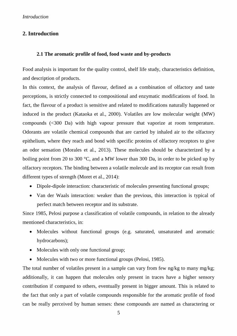
2. Introduction
2.1 The aromatic profile of food, food waste and by-products
Food analysis is important for the quality control, shelf life study, characteristics definition,
and description of products.
In this context, the analysis of flavour, defined as a combination of olfactory and taste
perceptions, is strictly connected to compositional and enzymatic modifications of food. In
fact, the flavour of a product is sensitive and related to modifications naturally happened or
induced in the product (Kataoka et al., 2000). Volatiles are low molecular weight (MW)
compounds (<300 Da) with high vapour pressure that vaporize at room temperature.
Odorants are volatile chemical compounds that are carried by inhaled air to the olfactory
epithelium, where they reach and bond with specific proteins of olfactory receptors to give
an odor sensation (Morales et al., 2013). These molecules should be characterized by a
boiling point from 20 to 300 °C, and a MW lower than 300 Da, in order to be picked up by
olfactory receptors. The binding between a volatile molecule and its receptor can result from
different types of strength (Moret et al., 2014):
• Dipole-dipole interaction: characteristic of molecules presenting functional groups;
• Van der Waals interaction: weaker than the previous, this interaction is typical of
perfect match between receptor and its substrate.
Since 1985, Pelosi purpose a classification of volatile compounds, in relation to the already
mentioned characteristics, in:
• Molecules without functional groups (e.g. saturated, unsaturated and aromatic
hydrocarbons);
• Molecules with only one functional group;
• Molecules with two or more functional groups (Pelosi, 1985).
The total number of volatiles present in a sample can vary from few ng/kg to many mg/kg;
additionally, it can happen that molecules only present in traces have a higher sensory
contribution if compared to others, eventually present in bigger amount. This is related to
the fact that only a part of volatile compounds responsible for the aromatic profile of food
can be really perceived by human senses: these compounds are named as charactering or
Introduction
6
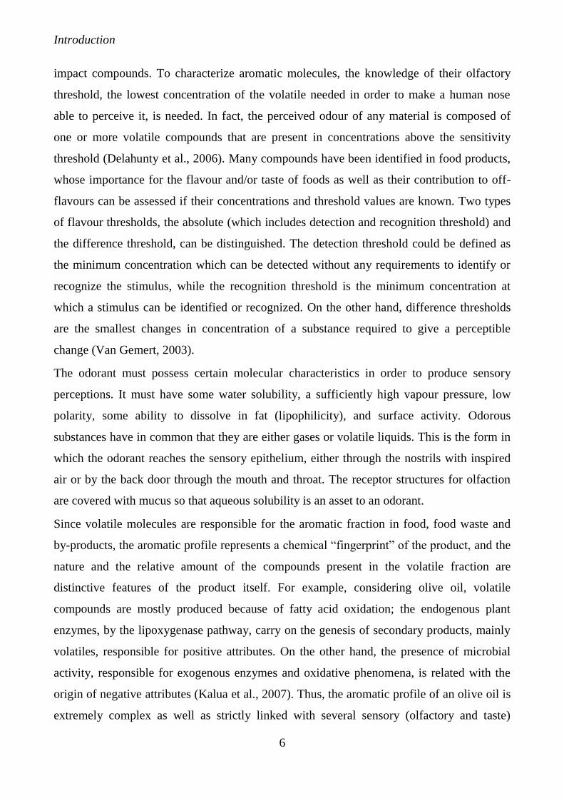
impact compounds. To characterize aromatic molecules, the knowledge of their olfactory
threshold, the lowest concentration of the volatile needed in order to make a human nose
able to perceive it, is needed. In fact, the perceived odour of any material is composed of
one or more volatile compounds that are present in concentrations above the sensitivity
threshold (Delahunty et al., 2006). Many compounds have been identified in food products,
whose importance for the flavour and/or taste of foods as well as their contribution to off-
flavours can be assessed if their concentrations and threshold values are known. Two types
of flavour thresholds, the absolute (which includes detection and recognition threshold) and
the difference threshold, can be distinguished. The detection threshold could be defined as
the minimum concentration which can be detected without any requirements to identify or
recognize the stimulus, while the recognition threshold is the minimum concentration at
which a stimulus can be identified or recognized. On the other hand, difference thresholds
are the smallest changes in concentration of a substance required to give a perceptible
change (Van Gemert, 2003).
The odorant must possess certain molecular characteristics in order to produce sensory
perceptions. It must have some water solubility, a sufficiently high vapour pressure, low
polarity, some ability to dissolve in fat (lipophilicity), and surface activity. Odorous
substances have in common that they are either gases or volatile liquids. This is the form in
which the odorant reaches the sensory epithelium, either through the nostrils with inspired
air or by the back door through the mouth and throat. The receptor structures for olfaction
are covered with mucus so that aqueous solubility is an asset to an odorant.
Since volatile molecules are responsible for the aromatic fraction in food, food waste and
by-products, the aromatic profile represents a chemical “fingerprint” of the product, and the
nature and the relative amount of the compounds present in the volatile fraction are
distinctive features of the product itself. For example, considering olive oil, volatile
compounds are mostly produced because of fatty acid oxidation; the endogenous plant
enzymes, by the lipoxygenase pathway, carry on the genesis of secondary products, mainly
volatiles, responsible for positive attributes. On the other hand, the presence of microbial
activity, responsible for exogenous enzymes and oxidative phenomena, is related with the
origin of negative attributes (Kalua et al., 2007). Thus, the aromatic profile of an olive oil is
extremely complex as well as strictly linked with several sensory (olfactory and taste)

Introduction
7
perceptions. Considering meat fermented product, as salami, aroma compounds can arise
from a complex pattern of chemical reactions involving the components of the matrix, like
oxidation of unsaturated fatty acids and microbiological metabolism of lipids, proteins and
carbohydrates (García-González et al., 2009, Bianchi et al., 2007).
Introduction
8
2.2 Sensory analysis of food
2.2.1 Anatomy and physiology of the five senses
Senses are physiological capacities of organisms that provide data for perception. The
senses and their operation, classification, and theory are overlapping topics studied by a
variety of fields, most notably neuroscience, cognitive psychology (or cognitive science)
and sensory analysis. The nervous system has a specific sensory system or organ, dedicated
to each sense.
2.2.1a The vision
Sight or vision is the capability of the eye(s) to focus and detect images of visible light on
photoreceptors in the retina of each eye that generates electrical nerve impulses for varying
colors, hues, and brightness. There are two types of photoreceptors: rods and cones. Rods
are very sensitive to light, but do not distinguish colors. Cones distinguish colors, but are
less sensitive to dim light. There is some disagreement as to whether this constitutes one,
two or three senses. Neuroanatomists generally regard it as two senses, given that different
receptors are responsible for the perception of color and brightness. Some argue that
stereopsis, the perception of depth using both eyes, also constitutes a sense, but it is
generally regarded as a cognitive (that is, post-sensory) function of the visual cortex of the
brain where patterns and objects in images are recognized and interpreted based on
previously learned information. This is called visual memory.
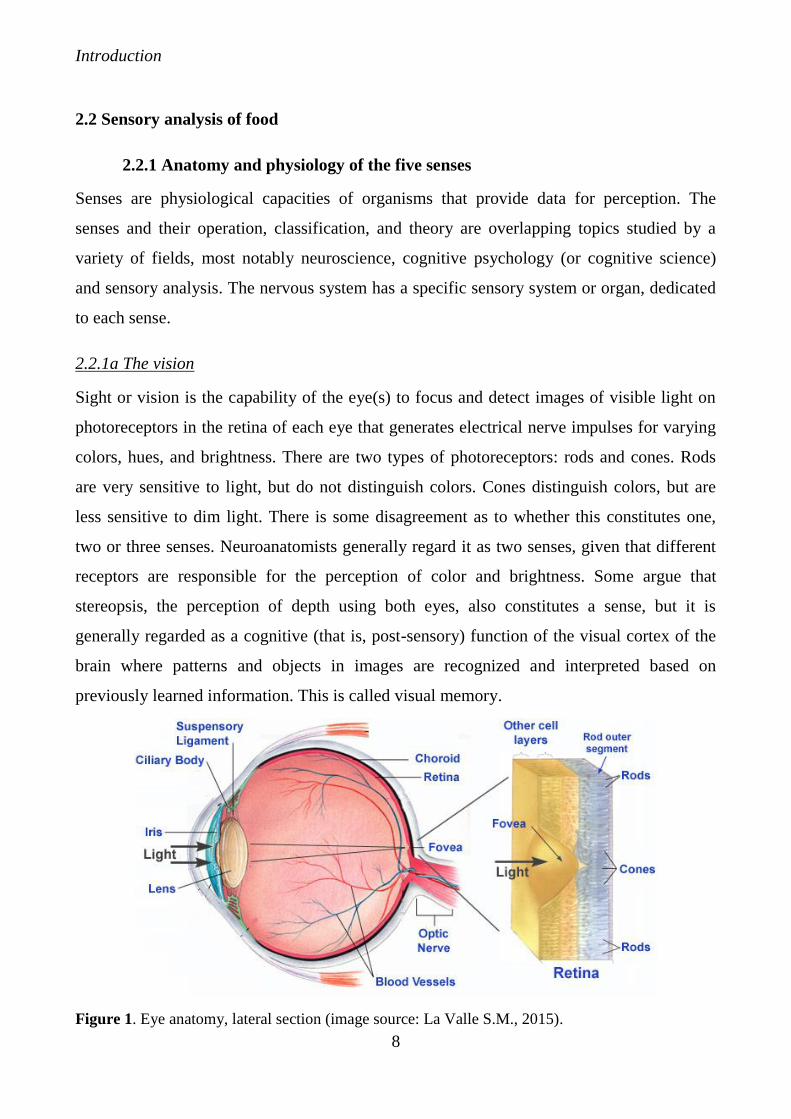
Figure 1. Eye anatomy, lateral section (image source: La Valle S.M., 2015).
Introduction
9
Figure 1 shows the anatomy of a human eye. The shape is approximately spherical, with a
diameter of around 24 mm and only slight variation among people. The cornea is a hard,
transparent surface through which light enters and provides the greatest optical power. The
rest of the outer surface of the eye is protected by a hard, white layer called the sclera.
All vision is based on the perception of electromagnetic rays. These rays pass through the
cornea in the form of light; the cornea focuses the rays as they enter the eye through the
pupil, the black aperture at the front of the eye. The pupil acts as a gatekeeper, allowing as
much or as little light to enter as is necessary to see an image properly. The pigmented area
around the pupil is the iris. Along with supplying a person's eye color, the iris is responsible
for acting as the pupil's stop, or sphincter. Two layers of iris muscles contract or dilate the
pupil to change the amount of light that enters the eye. Behind the pupil is the lens, which
is similar in shape and function to a camera lens. Together with the cornea, the lens adjusts
the focal length of the image being seen onto the back of the eye, the retina. Visual
reception occurs at the retina where photoreceptor cells called cones and rods give an image
color and shadow. The image is transduced into neural impulses and then transferred
through the optic nerve to the rest of the brain for processing. The visual cortex in the brain
interprets the image to extract form, meaning, memory and context (Crescitelli, 1960).
In food products, especially meats, fruits and vegetables, the consumer often assesses the
initial quality of the product by its color and appearance; thus, appearance and color are the
primary indicators of perceived quality. The visual characteristics of a product can affect the
consumers’ perceptions of other sensory modalities in that food as well (Lawless et al.,
2010). Together with touch and smell senses, the sight is responsible for texture attributes
perception (Lawless et al., 2010) that has been defined as “the sensory and functional
manifestation of the structural, mechanical and surface properties of foods detected through
the senses of vision, hearing and touch” (Szczesniak, 2002).
Introduction
10
2.2.1b The smell
The human sense of smell has often been regarded as the least refined of all the human
senses and far inferior to that of other animals. In fact, Aristotle (384–322 BC) blames this
lack of finesse on the ducts in the human nose and claims that people who have noses with
narrower ducts have a keener sense of smell, but he cites no experimental evidence for this
assertion (Aristotle in Problemata XXXIII, and in De Sensu et Sensibili in Parva Naturalia).
Moreover, the Roman philosopher Lucretius (99–55 BC) focused on the shape of the
particles as conveying the quality of the odour and speculated on human olfaction by
considering the nature and role of the odorant particles (Lucretius in De Rerum Natura).
Also, the sense of smell is intimately linked with our emotions and aesthetics, but, despite
the importance of odour, there is a lack of a suitable vocabulary to describe odours with
precision. This is recognised by Plato in Timaeus: “the varieties of smell have no name, but
they are distinguished only as painful and pleasant” (Brattoli et al., 2011). The identification
of primary olfactory submodalities has been attempted many times. The first serious effort
at identification was made by Linnaeus, the Swedish botanist, in 1756.
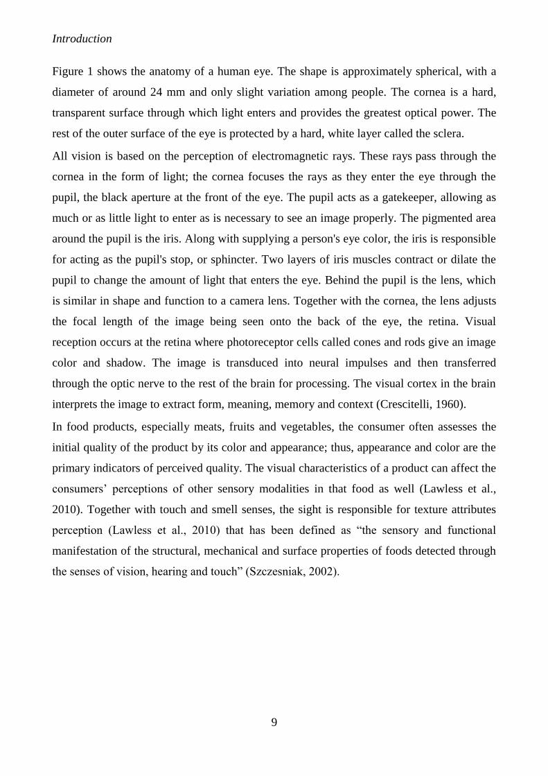
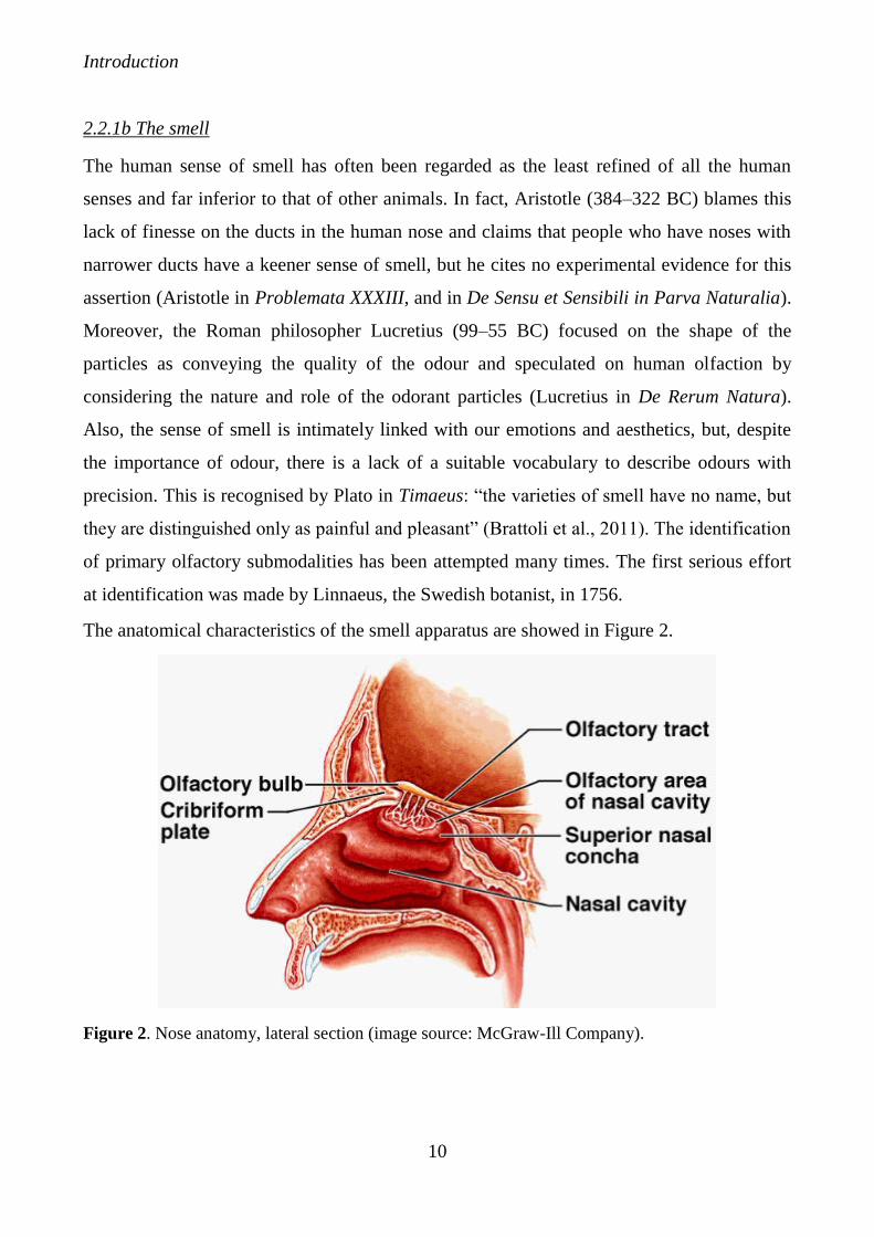
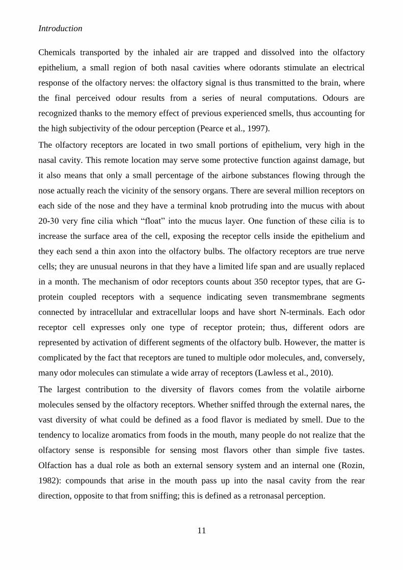
The anatomical characteristics of the smell apparatus are showed in Figure 2.
Figure 2. Nose anatomy, lateral section (image source: McGraw-Ill Company).
Introduction
11
Chemicals transported by the inhaled air are trapped and dissolved into the olfactory
epithelium, a small region of both nasal cavities where odorants stimulate an electrical
response of the olfactory nerves: the olfactory signal is thus transmitted to the brain, where
the final perceived odour results from a series of neural computations. Odours are
recognized thanks to the memory effect of previous experienced smells, thus accounting for
the high subjectivity of the odour perception (Pearce et al., 1997).
The olfactory receptors are located in two small portions of epithelium, very high in the
nasal cavity. This remote location may serve some protective function against damage, but
it also means that only a small percentage of the airbone substances flowing through the
nose actually reach the vicinity of the sensory organs. There are several million receptors on
each side of the nose and they have a terminal knob protruding into the mucus with about
20-30 very fine cilia which “float” into the mucus layer. One function of these cilia is to
increase the surface area of the cell, exposing the receptor cells inside the epithelium and
they each send a thin axon into the olfactory bulbs. The olfactory receptors are true nerve
cells; they are unusual neurons in that they have a limited life span and are usually replaced
in a month. The mechanism of odor receptors counts about 350 receptor types, that are G-
protein coupled receptors with a sequence indicating seven transmembrane segments
connected by intracellular and extracellular loops and have short N-terminals. Each odor
receptor cell expresses only one type of receptor protein; thus, different odors are
represented by activation of different segments of the olfactory bulb. However, the matter is
complicated by the fact that receptors are tuned to multiple odor molecules, and, conversely,
many odor molecules can stimulate a wide array of receptors (Lawless et al., 2010).
The largest contribution to the diversity of flavors comes from the volatile airborne
molecules sensed by the olfactory receptors. Whether sniffed through the external nares, the
vast diversity of what could be defined as a food flavor is mediated by smell. Due to the
tendency to localize aromatics from foods in the mouth, many people do not realize that the
olfactory sense is responsible for sensing most flavors other than simple five tastes.
Olfaction has a dual role as both an external sensory system and an internal one (Rozin,
1982): compounds that arise in the mouth pass up into the nasal cavity from the rear
direction, opposite to that from sniffing; this is defined as a retronasal perception.
Introduction
12
Together with the visual characteristics of a product, the smell is responsible of the first
reaction of human being to a food (Pagliarini, 2002).
2.2.1c The taste
Taste is the ability to respond to dissolved molecules and ions called tastants.
The sensation of taste includes five established basic tastes: sweetness, sourness, saltiness,
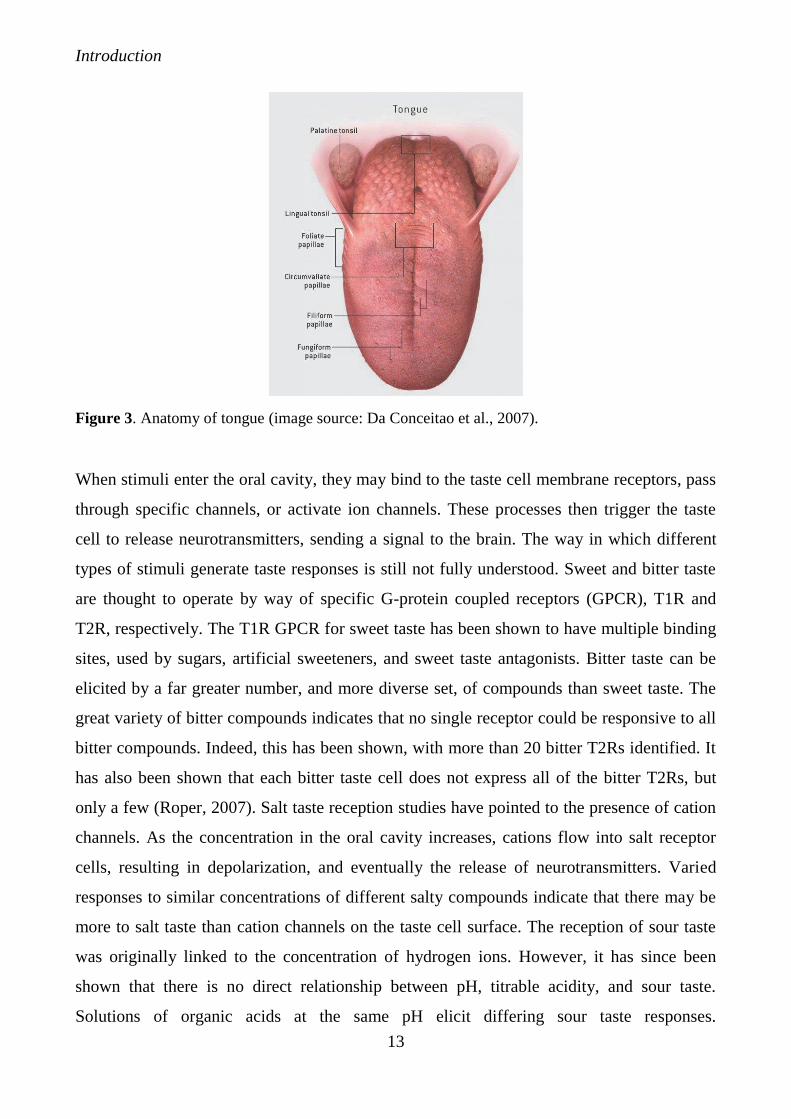
bitterness, and umami (Korsmeyer, 2002). The taste system consists of 3 types of taste
papillae (Figure 3), on which taste buds are located. Fungiform papillae, which are
mushroom shaped structures, are located towards the front of the tongue. Each fungiform
papillae usually contains 3-5 taste buds. Circumvallate papillae are located towards the back
of the tongue, and unlike fungiform papilla, they each contain more than 100 taste buds. The
ridges and grooves located along the sides of the tongue are foliate papillae. Like
circumvallate papillae, foliate papillae also contain more than 100 taste buds each. A fourth
type of papillae, filiform, also exists, but does not contain any taste buds. Each taste bud
consists of 30-100 taste receptor cells. Taste receptor cells are long, thin cells oriented
perpendicular to the surface of the tongue. One end of the taste each taste receptor cell is
exposed to the oral cavity and has microvilli on its surface to increase contact with stimuli.
The opposing end of the taste receptor cell contacts nerve fibers which feed into the
glossopharyngeal nerve, chorda tympani or vagal nerve, depending on the location of the
taste bud (Da Conceitao et al., 2007).
Introduction
13
Figure 3. Anatomy of tongue (image source: Da Conceitao et al., 2007).
When stimuli enter the oral cavity, they may bind to the taste cell membrane receptors, pass
through specific channels, or activate ion channels. These processes then trigger the taste
cell to release neurotransmitters, sending a signal to the brain. The way in which different
types of stimuli generate taste responses is still not fully understood. Sweet and bitter taste
are thought to operate by way of specific G-protein coupled receptors (GPCR), T1R and
T2R, respectively. The T1R GPCR for sweet taste has been shown to have multiple binding
sites, used by sugars, artificial sweeteners, and sweet taste antagonists. Bitter taste can be
elicited by a far greater number, and more diverse set, of compounds than sweet taste. The
great variety of bitter compounds indicates that no single receptor could be responsive to all
bitter compounds. Indeed, this has been shown, with more than 20 bitter T2Rs identified. It
has also been shown that each bitter taste cell does not express all of the bitter T2Rs, but
only a few (Roper, 2007). Salt taste reception studies have pointed to the presence of cation
channels. As the concentration in the oral cavity increases, cations flow into salt receptor
cells, resulting in depolarization, and eventually the release of neurotransmitters. Varied
responses to similar concentrations of different salty compounds indicate that there may be
more to salt taste than cation channels on the taste cell surface. The reception of sour taste
was originally linked to the concentration of hydrogen ions. However, it has since been
shown that there is no direct relationship between pH, titrable acidity, and sour taste.
Solutions of organic acids at the same pH elicit differing sour taste responses.
Introduction
14
Likewise, solutions of organic acids of the same normality also result in difference sour
taste responses. It is obvious that undissociated acids play a role in sour taste, but the
mechanism is unclear. Umami is an oral sensation stimulated by salts of glutamic or aspartic
acids, roughly translated by japanese as “delicious taste”, and attributes to the taste of
monosodium glutamate (MSG) and ribosides such as salts of inosine monophosphate and
guanine monophosphate (Lawless et al., 2010).
2.2.1d The touch
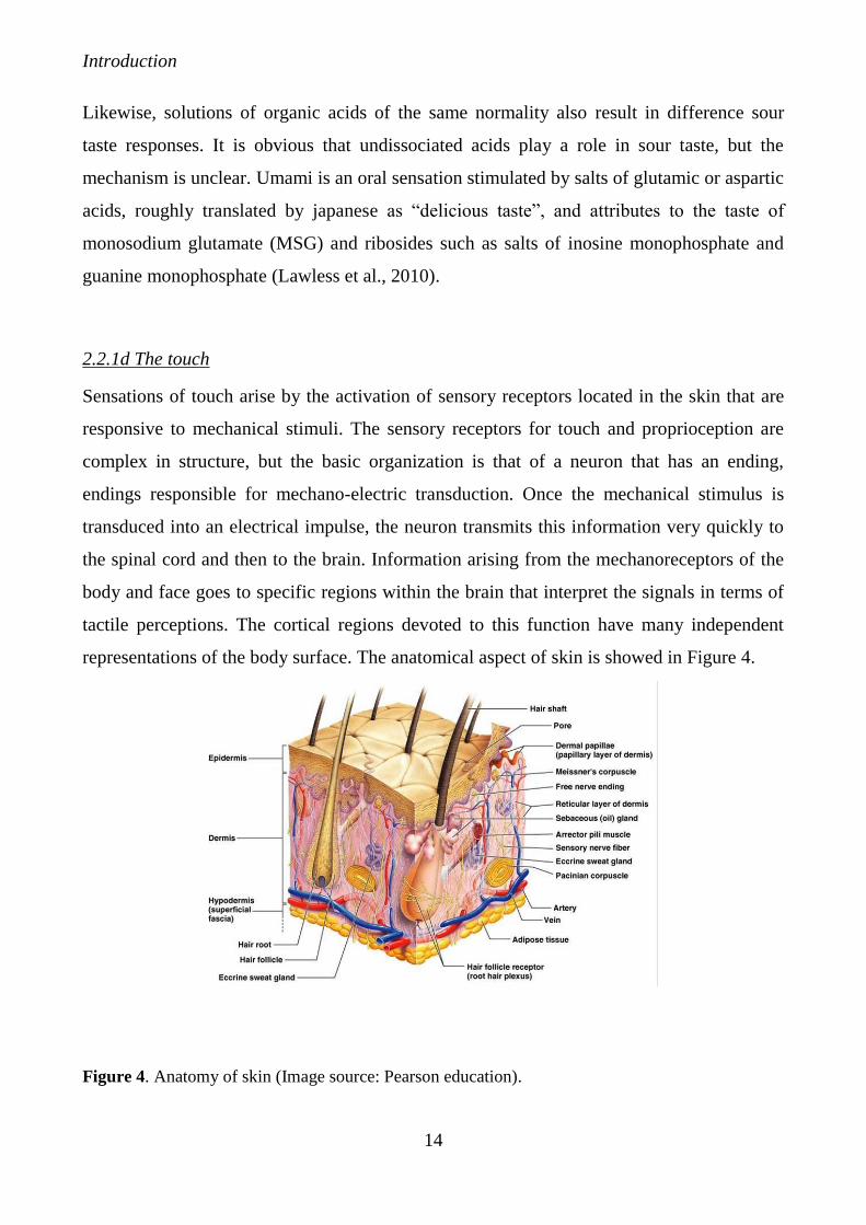
Sensations of touch arise by the activation of sensory receptors located in the skin that are
responsive to mechanical stimuli. The sensory receptors for touch and proprioception are
complex in structure, but the basic organization is that of a neuron that has an ending,
endings responsible for mechano-electric transduction. Once the mechanical stimulus is
transduced into an electrical impulse, the neuron transmits this information very quickly to
the spinal cord and then to the brain. Information arising from the mechanoreceptors of the
body and face goes to specific regions within the brain that interpret the signals in terms of
tactile perceptions. The cortical regions devoted to this function have many independent
representations of the body surface. The anatomical aspect of skin is showed in Figure 4.
Figure 4. Anatomy of skin (Image source: Pearson education).
Introduction
15
The sense of touch is responsible for the perception of textural characteristics of products.
The textural properties of a product are linked with its compositional and mechanical
properties; the evaluation of these aspect is defined as “all the mechanical, geometrical and
surface attributes of a product perceptible by mechanical and tactile receptors” (ISO 5492).
2.2.1e The hearing
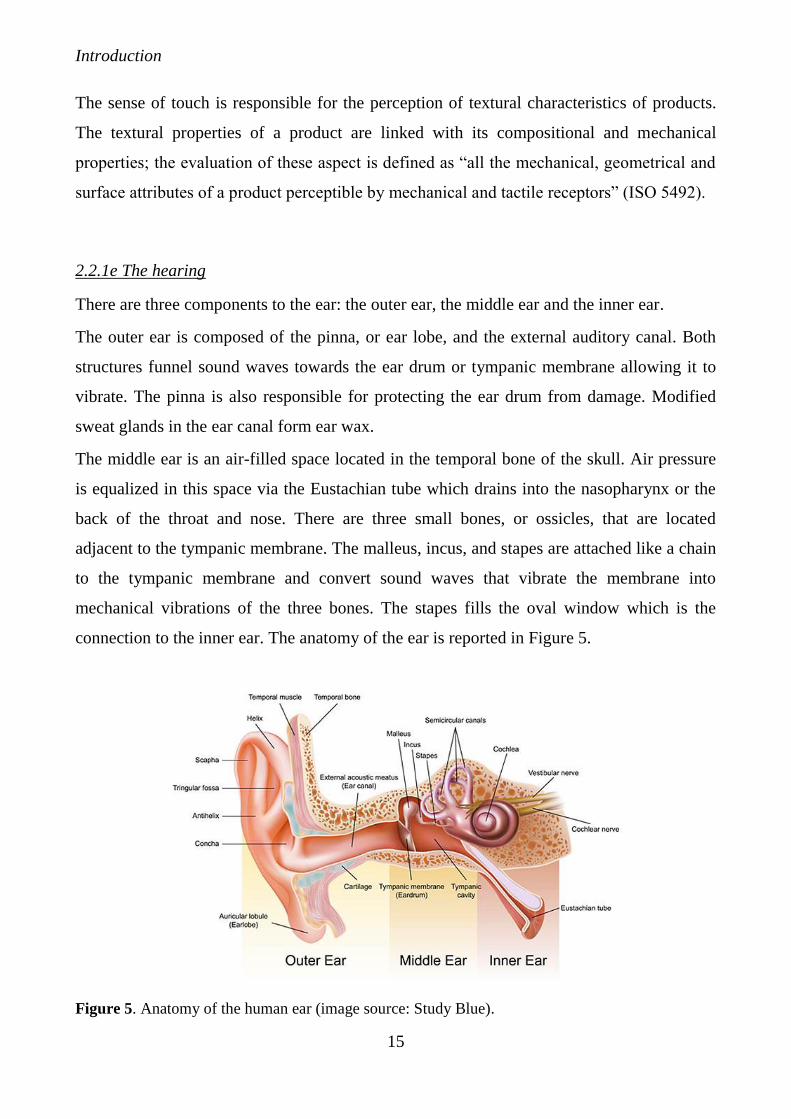
There are three components to the ear: the outer ear, the middle ear and the inner ear.
The outer ear is composed of the pinna, or ear lobe, and the external auditory canal. Both
structures funnel sound waves towards the ear drum or tympanic membrane allowing it to
vibrate. The pinna is also responsible for protecting the ear drum from damage. Modified
sweat glands in the ear canal form ear wax.
The middle ear is an air-filled space located in the temporal bone of the skull. Air pressure
is equalized in this space via the Eustachian tube which drains into the nasopharynx or the
back of the throat and nose. There are three small bones, or ossicles, that are located
adjacent to the tympanic membrane. The malleus, incus, and stapes are attached like a chain
to the tympanic membrane and convert sound waves that vibrate the membrane into
mechanical vibrations of the three bones. The stapes fills the oval window which is the
connection to the inner ear. The anatomy of the ear is reported in Figure 5.
Figure 5. Anatomy of the human ear (image source: Study Blue).
Introduction
16
The ear canal acts as a resonating tube and actually amplifies sounds at between 3,000 and
4,000 Hz adding to the sensitivity (and susceptibility to damage) of the ear at these
frequencies. The ear is very sensitive and responds to sounds of very low intensity, to
vibrations which are hardly greater than the natural random movement of molecules of air.
To do this the air pressure on both sides of the tympanic membrane must be equal. The
Eustachian tube provides the means of the pressure equalization. It does this by opening for
short periods, with every 3rd or 4th swallow; if it were open all the time one would hear
one's own every breath. Because the lining membrane of the middle ear is a respiratory
membrane, it can absorb some gases, so if the Eustachian tube is closed for too long it
absorbs carbon dioxide and oxygen from the air in the middle ear, thus producing a negative
pressure. This may produce pain (as experienced if the Eustachian tube is not unblocked
during descent of an aeroplane). The middle ear cavity itself is quite small and the mastoid
air cells act as an air reservoir cushioning the effects of pressure change. The outer and
middle ears serve to amplify the sound signal. The sense of hearing is involved in sensory
evaluation of food for all of the attributes related with vibration: during biting, man
vibrations are produced and can be associated with attributes like crunchy (e.g. biscuits or
chips) (Vickers, 1991).
Introduction
17
2.2.2 Sensory analysis: definition and methodologies
Sensory analysis is “a scientific discipline used to evoke, measure, analyse and interpret
those responses to products that are perceived by the senses of sight, smell, touch, taste and
hearing” (Stone et al., 2012).
The definition represents a conscious to be as inclusive as is possible within the framework
of food evaluation, with the word “food” used as global, indicating an ingredient is a food, a
beverage is a food, and so forth (O’Sullivan, 2016). Sensory characterization provides a
representation of the qualitative and quantitative aspects of human perception, enabling
measurement of the sensory reaction to the stimuli resulting from the use of a product and
allowing correlations to the other parameters (Varela et al., 2012; Lawless et al, 2010;
Murray et al., 2001). Globally, sensory analysis represents the definition and scientific
measurement of a product perceived by the five senses. This definition fits both with
qualitative and quantitative methods and does not discriminate the assessors according to
their capability and awareness of the methods or the test in relation with the final objective
of a study. In fact, only a correct pre-selection of the method and the judges, as a function of
the real objective of a sensory investigation, is the correct way to proceed with sensory
analysis, giving it the real significance of a scientific discipline. Sensory analysis answers to
questions that embrace quality from different points of view: description, preference and
discrimination: all of these answers are useful to communicate and provide an input in
decision making (Carpenter et al., 2012). In general, three types of sensory testing are
commonly used: i) affective, hedonic tests that involve consumers and concern subjective
and acceptance issues, for these tests judges should be untrained; ii) discrimination, these
are analytic tests that deal with the investigation product perceptible differences and request
judges that could be trained and screened for their sensory acuity; iii) descriptive, analytical
tests oriented to the description of specific sensory characteristics. This last category needs
trained or higly trained judges, previously screened for their acuity and motivation (Lawless
et al., 2010).
Introduction
18
2.2.2a Discrimination methods
Discrimination tests should be used when the sensory specialist wants to determine whether
two samples are perceptibly different (Stone et al., 2004). Analysis is usually based on the
statistics of frequencies and proportions (counting right and wrong questions). From the
results of these tests differences based on the proportions of persons who are able to choose
a test product correctly from a set of similar products can be inferred. A classic example of
this test was the triangle procedure, where two products are equal and the third one differs,
for example, in the amount of one ingredient but it’s produced with the same recipe and in
the same way. Judges would be asked to pick the different sample from among the three.
Ability to discriminate differences would be inferred from consistent correct choices above
the level expected by chance. A product preference test can determine if consumers prefer
one product when compared to another product. Another multiple choice different test was
developed by Peryam and Swartz (Peryam et al., 1950) for purposes of quality control, and
it’s named duo-trio test. In this test, two test samples and a reference samples are given to
untrained assessors. One of the test samples matches the reference while the other one
comes from a different product/batch/process. The participant try to match the correct
sample to the reference, with a chance of probability of one-half. Another widespread test is
the paired comparison, where participants are asked to choose which, among two samples,
is the strongest or more intense in a given attribute. Partly due to the fact that panelist’s
attention is directed to a specific attribute, this test is very sensitive to differences (Lawless
et al., 2010). Simple difference tests have proven very useful in application and are in
widespread use today. Typically, a discrimination test will be conducted by 25-40
participants who have been screened for their sensory acuity to common product differences
and who are familiar with the test procedures. A replicate test is often performed while the
respondents are present in the sensory test facility. The popularity of these tests is also due
the simplicity of data analysis: statistical tables of binomial distribution give the minimum
number of correct responses needed to conclude statistical significance as a function of the
number of participants.
Introduction
19
2.2.2b Affective methods
These tests have the main objective of quantify the degree of linking or disliking of a
product. The most straightforward approach to this method is to offer people a choice
among alternative products and see if there is a clear preference from the majority of
respondents. The problem with these tests is that they do not give information on the
magnitude of liking or disliking from respondents. The hedonic scale, frequently used for
these tests, was developed in 50’s (Jones et al., 1955) and was constituted by a 9-point scale
for liking with a centered neutral category and attempted to produce scale point labels with
adverbs that represents psychologically equal steps or changes in hedonic tone. Typically, a
hedonic test involves 75-150 participants, that have to be regular consumers of the product
tested. Consumers are given several alternative versions of the product and the large number
of interviewed compensates the effect of individual preferences, ensuring statistical power
and test sensitivity. This also provide an opportunity to look for segments of people who
may like different styles of a product, for example, different colors or flavors. This approach
with consumers has the aim to indagate their preferences, asking them to indicate their most
liked product. Although these tests appear straightforward and simple, several complications
are encountered in the methods, notably how to treat replicated data and how to analyse data
that include a “no-preference” option as a response (Lawless et al., 2010).
Introduction
20
2.2.2c Descriptive analysis (DA)
Classic or generic descriptive analysis is the gold standard technique in sensory science
(Lawless et al., 2010). Sensory characterization is extensively applied in the industry for the
development and marketing of new products, the reformulation of existing products, the
optimization of manufacturing processes, the monitoring of sensory characteristic of the
product present on the market, the implementation of sensory quality assurance programs,
the establishment of relationship between sensory and instrumental methods and for
estimating sensory shelf life (Varela et al., 2014).
These methods are used for quantifying the perceived intensities of different attributes
detected in a sample. In the late 1940s the first method to do this with a panel of trained
judges was established and named Flavor Profile® (Caul, 1957). This first approach to
descriptive analysis represents a flexible tool, useful to solve problem of off-flavors in
nutritional capsules and questions about the sensory contribution of sodium glutamate in
different processed foods. This method enabled panellists to characterize all of the notes by
means of a category scale and noting their order of appearance. Subsequently, in the 1970s,
a refined method, known as Texture profile, to quantify food texture, much as the flavour
profile had enabled the quantification of flavour properties (Szezesniak et al., 1975). Using
Texture Profile, rheological and tactile properties of foods, and how these change every
time during biting, could be characterized, by means of a fixed set of force-related and
sharpe-related attributes. After that, other approaches were proposed for descriptive analysis
of food. In 1974, the method named Quantitative Descriptive Analysis (QDA®) enlarged the
possibility of description, in terms of attributes, to all the sensory perception, and not only to
taste and texture (Stone et al., 2012). To the best of our knowledge, descriptive analysis has
proved to be the most comprehensive and informative sensory evaluation tool. In fact, this
method can be applied to a wide variety of product changes and research questions in food
product development. Additionally, the information acquired can be related to consumer
acceptance information but also to instrumental measurement, by means of statistical
techniques such as regression and correlation. In fact, sensory descriptive analysis acts like
a bridge between different areas of research, product development and consumer science,
providing a link between the products characteristics and consumer perception.

Introduction
21
Before performing a DA, few keypoint should be fixed: the selection of judges (and their
numerosity), the training phase, the selection of attributes and references have to be pointed
out, togheter with a certain number of replicates when real samples are evaluated.
Panel selection. The panellists must be motivated and interested on the research activity in
which they are going to be involved in. A number of ten to twelve judges is recommended.
Regarding the previous screening of panellists, researchers are divided: many encourage this
(Barcenas et al., 2000; Noronha et al., 1995), while others found that the screening seems to
decrease panel performance, especially when the process is onerous and protracted
(Nachtsheim et al., 2012).
Term generation and reference standard. In this process the panellists are enrolled in
determining, through consensus, the attributes that discriminate among the samples. On the
first day, judges are served many samples, chosen to be as different as possible, in order to
define, individually and quietly, a list of attributes that must be actionable; thus, reference
standard could be selected for each of them. After this first moment of individual work, the
panellists start a discussion, guided by the panel leader, and reading the attributes they
selected. The panel leader works as a communication facilitator without involvement and
interference with panel discussions. In this way, terms that refer to the same meaning can be
grouped and only one among each group will be selected, in order to avoid redundancy.
At the next training session, panellists are given another subset of samples and the process is
repeated; additionally, potential reference standards (selected from literature or previous
experiences) are showed to the judges, to anchor the attributes. References can be used for
generating sensory terminologies, especially when panellists are confused and disagree with
each other on some sensory attributes. This process is repeated as many time as it is needed,
in order to ensure that all the potential terms have been listed. Once the attribute list has
been completed, the training session involve making sure that the entire panel is
comfortable with the specific reference standards; subsequently, panellists are shown the
profile sheet set up with all the terms selected.
Evaluation of samples. Once the panel has been trained and tested, the actual evaluation of
samples can start. It is usual that this process occurs in individual, temperature and light
controlled booths (Lawless et al., 2010) and data collection could be done by means of

Introduction
22
paper profile sheet data acquisition or by computerized system. Panelists must be made to
feel welcome and appreciated during the data acquisition phase, to ensure continued
motivation and interest. It is not unusual to serve them some snacks as a token of
appreciation after they complete their sensory sessions. In certain situations, it may also be
appropriated to pay panellists (Varela et al., 2014).
Introduction
23
2.3 Methods for volatile compounds analysis
In general, the analytical methods used for the evaluation of volatile compounds involve all
the steps of the general analytical process such as sampling, sample preparation, separation,
identification, quantification and data analysis (Morales et al., 1992).
Methods for volatile compounds determination reported in literature can be divided in two
different groups, according to their eventual requirement for a pre-concentration of
compounds, in order to have volatiles in a concentration higher than the quantification limit
of the method itself (Angerosa et al., 2004; Angerosa, 2002).
This additional requirement of pre-concentration phase is related to the complexity of
headspace in many food matrix (e.g. olive oil); moreover, volatiles can contribute to the
aromatic profile of a sample even being present in a very low concentration (Escuderos et
al., 2007).
The main techniques that do not necessary need a pre-concentration of compounds are: the
direct injection, the static headspace analysis (SHS) (Escuderos et al., 2007) and the thermal
desorption (TD). The latter is represented by the direct desorption of analytes from an
appropriate adsorbent, avoiding intermediate extraction and concentration steps prior to
analysis. As a consequence, TD methods are characterised by a higher sensitivity, which
may provide shorter sampling times or lower sampling volumes.
On the other hand, techniques related to an enrichment/pre-concentration of the samples are
frequently used and represented by (Vichi et al., 2010; Escuderos et al., 2007):
• Dynamic Headspace Analysis (DHS): volatile compounds are dragged by an inert gas
flow, previously gurgled through the heated sample, and subsequently trapped in an
adsorbent suitable material (active carbon, polymers, solvents, cryogenic traps).
Molecules are then desorbed by elution with a suitable heated solvent and gas
chromatographically analysed;
• Supercritical Fluid Extraction (SFE): this tecnique advantages are time reduction and
high efficiency extraction;
• Stir Bar Sorptive Extraction (SBSE): based upon sorption, which is a form of
partition based upon the analyte's dissolution in a liquid-retaining polymer from a
liquid or vapor sample, thus, originating a bulk retention (Bicchi et al., 2000).

Introduction
24
• Solid-Phase Micro Extraction (SPME): SPME techniques was developed as an
alternative to the dynamic headspace analysis and is based on the use of a holder,
comparable to a syringe that contains a steel needle enclosing a retractable
chemically inert silica fibre. The fibre is coated with an adsorbent material
(stationary liquid or solid phase) which is exposed, for a predefined time, in the
sample headspace. Molecules are then desorbed and subsequently gas
chromatographically analysed.
Introduction
25
2.3.1 Gas chromatographic analysis of volatile compounds
The chromatographic technique was applied for the first time by Tswett, a Russian-Italian
botanist, during his research on plant pigments, in 1903. He used liquid-adsorption column
chromatography with calcium carbonate as adsorbent and petrol ether/ethanol mixtures as
eluent to separate chlorophylls and carotenoids.
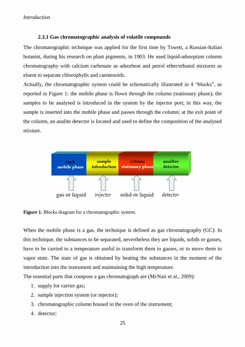
Actually, the chromatographic system could be schematically illustrated in 4 “blocks”, as
reported in Figure 1: the mobile phase is flown through the column (stationary phase); the
samples to be analysed is introduced in the system by the injector port; in this way, the
sample is inserted into the mobile phase and passes through the column; at the exit point of
the column, an analite detector is located and used to define the composition of the analysed
mixture.
Figure 1. Blocks diagram for a chromatographic system.
When the mobile phase is a gas, the technique is defined as gas chromatography (GC). In
this technique, the substances to be separated, nevertheless they are liquids, solids or gasses,
have to be carried to a temperature useful to transform them to gasses, or to move them to
vapor state. The state of gas is obtained by heating the substances in the moment of the
introduction into the instrument and maintaining the high temperature.
The essential parts that compose a gas chromatograph are (McNair et al., 2009):
1. supply for carrier gas;
2. sample injection system (or injector);
3. chromatographic column housed in the oven of the instrument;
4. detector;
Introduction
26
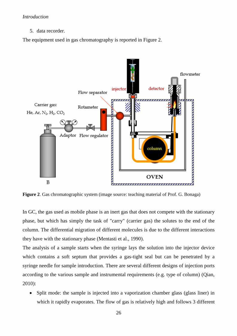
5. data recorder.
The equipment used in gas chromatography is reported in Figure 2.
Figure 2. Gas chromatographic system (image source: teaching material of Prof. G. Bonaga)
In GC, the gas used as mobile phase is an inert gas that does not compete with the stationary
phase, but which has simply the task of "carry" (carrier gas) the solutes to the end of the
column. The differential migration of different molecules is due to the different interactions
they have with the stationary phase (Mentasti et al., 1990).
The analysis of a sample starts when the syringe lays the solution into the injector device
which contains a soft septum that provides a gas-tight seal but can be penetrated by a
syringe needle for sample introduction. There are several different designs of injection ports
according to the various sample and instrumental requirements (e.g. type of column) (Qian,
2010):
• Split mode: the sample is injected into a vaporization chamber glass (glass liner) in
which it rapidly evaporates. The flow of gas is relatively high and follows 3 different
Introduction
27
ways: a part (purge line) touches and cleans the silicone septum, a part (sample line)
carries the sample vapor into the column and a part (split-line) carries the sample
vapor to the output of the separator (splitter), regulated by a needle valve (split
valve). The relationship between the separator flow (split flow) and the column flow
is called "split ratio" and is what is regulated by the split valve; it determines the
amount of sample that actually enters the chromatographic column.
• Splitless mode: the sample is injected into a glass liner chamber with the splitter
valve closed. The process of volatilization of the sample, therefore, is progressive
from the point of injection and the transfer to the column of the volatilized solutes is
slow; a dditionally, the solutes are mixed with solvent. After a certain time (splitless
period), during which only the purge line remains open, the split line is opened both
to split a part of the solutes and to make the other part flows towards the column. To
minimize the loss of the sample components by condensation on the top of the
injector, the temperature is maintained constant from the septum down thanks to an
additional heater.
• On-column mode: the "on-column" injectors could be equipped with a manual
introduction valve (by rotation) or an introduction septum that accommodates the
syringe needle into a needle channel. The mixture of solute enters the glass liner with
the injector maintained at room temperature by a flow of cold air; subsequently, the
injector is heated to obtain the evaporation of the solvent and vaporization of the
sample components, which are transported by the gas inside the column.
The GC column may be classified either as packed or capillary (open tubular). The second
type may be viewed as an alternative for the packed column, being the most popular. In the
capillary column, the stationary phase could be a thin film of liquid that coats the inside
wall (wall-coated capillary colun – WCOT), an adsorbed layer of a very small solid support
coated with a liquid phase (support-coated open-tubolar column – SCOT)or a porous layer
of a solid adsorbent (porous layer open-tubular column – PLOT).
The detectors are able to return both a full signal or a differential signal.
The integral signal produces a cumulative chromatogram, represented by a series of ramps
which correspond to the solutes separated by the column, with an order that corresponds to
their elution order. The differential signal produces a chromatogram represented by a series
Introduction
28
of peaks which correspond to the solutes separated by the column as a function of their
retention time. The detectors generally used for the GC analysis are:
• Thermal Conductivity Detector (TCD): is based on the principle that a gas, flowing
out of a heated filament reduces the filament temperature by removing part of the
heat. The amount of heat removed depends on the flow and the thermal conductivity
of the gas flowing. In a gas mixture, therefore, it depends on the thermal conductivity
of each component (solute, solvent, carrier gas) and the partial pressure of each of
them. The TCD body dual cell is a metal block of mass and high thermal inertia in
which two cells are obtained. It is thermostatically controlled to a temperature of
about 50 °C higher than the maximum of the column, so as to avoid condensation
phenomena.
• Flame Ionization Detector (FID): this detector is one of the most commonly used. In
this case the detection is based on the ions formed during combustion of organic
compounds in a hydrogen flame. The generation of these ions is proportional to the
concentration of organic species in the sample gas stream. The formation of positive
ions and electrons produces their migration towards the cathode and towards the
anode respectively, with the production of a stream of charged, as an electric current
capable of providing a signal. The FID response doesn’t depend on the concentration
of the solute, but on the number of carbon atoms present in the molecule.
• Electron Capture Detector (ECD): this detector is based on the primary ionization of
the substances for emission of β- particles (fast electrons) by a weak emitter, such as
the radioactive isotope 63Ni. The carrier gas carries the solutes containing
electronegative groups (halogens, peroxides, quinones, nitro, etc.) to the detector.
The anions that are formed have a reduced mobility to the anode (than that of the
electrons towards the anode) and, therefore, a modest electrical conductivity, in order
to not alter the value of the background.
• Nitrogen Phosphorous Detector (NPD): is based on a FID in the presence of alkaline
salts (silicate of Rb or Cs). The flame vaporizes and ionizes the Rb of the silicate,
with formation of Rb+ ions and electrons. The Rb+ ions migrate to the cathode, where
it will discharge and re-form the salt, while the electrons are attracted by the anode. If
the difference of potential between the two electrodes and the flame temperature are
Introduction
29
constant, there is a balance which corresponds to a constant electric current between
the two electrodes. When the solutes that elute from the column reach the detector, if
some of them contain the atoms of N, P or halogen, they are decomposed by the
flame and form of radical that selectively reacts with Rb+ ions present in the flame,
removing them from the balance of ionization of Rb. To restore this balance, the
system comprises further vaporization and ionization of the silicate Rb, with the
formation of new electrons. The net balance of these processes is, therefore, an
increase of the electric current in the circuit, ie the signal that reveals the solutes.
Additionally, one of the most diffused detector, frequently coupled to gas chromatographic
system, is the mass spectrometer (MS). This application is able to convert individual
molecules into ions, so that they can be moved about and manipulated by external electric
and magnetic fields. Because ions are very reactive and short-lived, their formation and
manipulation must be conducted in a vacuum. The pressure under which ions may be
handled is roughly 10-5 to 10-8 torr (less than a billionth of an atmosphere). Each of the three
tasks listed above may be accomplished in different ways. In one common procedure,
ionization is effected by an high energy beam of electrons, and ion separation is achieved by
accelerating and focusing the ions in a beam, which is then bent by an external magnetic
field. The ions are then detected (qualitatively and quantitatively) electronically and the
resulting information are shown in a mass spectrum (Figure 3). In GC–MS systems, the
analytes may be ionized in a number of ways but, most often, electron ionization (EI) is
used especially for automated screening analysis. Cations formed by the electron
bombardment are pushed away by a charged repeller plate (anions are attracted to it), and
accelerated toward other electrodes, having slits through which the ions pass as a beam.
Some of these ions fragment into smaller cations and neutral fragments. A perpendicular
magnetic field deflects the ion beam in an arc whose radius is inversely proportional to the
mass of each ion. Lighter ions are deflected more than heavier ions. By varying the strength
of the magnetic field, ions of different mass can be focused progressively on a detector fixed
at the end of a curved tube (also under a high vacuum). When an high energy electron
collides with a molecule it often ionizes it by knocking away one of the molecular electrons
(either bonding or non-bonding). Residual energy from the collision may cause the
molecular ion to fragment into neutral pieces and smaller fragment ions. The molecular ion
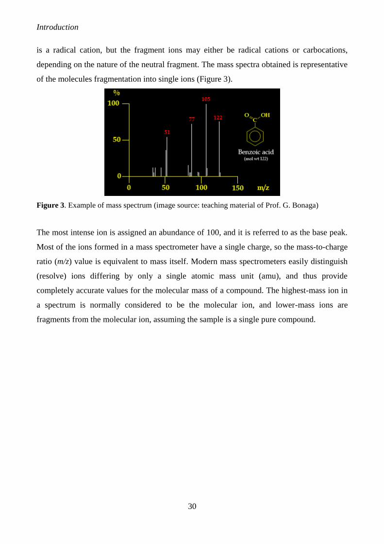
Introduction
30
is a radical cation, but the fragment ions may either be radical cations or carbocations,
depending on the nature of the neutral fragment. The mass spectra obtained is representative
of the molecules fragmentation into single ions (Figure 3).
Figure 3. Example of mass spectrum (image source: teaching material of Prof. G. Bonaga)
The most intense ion is assigned an abundance of 100, and it is referred to as the base peak.
Most of the ions formed in a mass spectrometer have a single charge, so the mass-to-charge
ratio (m/z) value is equivalent to mass itself. Modern mass spectrometers easily distinguish
(resolve) ions differing by only a single atomic mass unit (amu), and thus provide
completely accurate values for the molecular mass of a compound. The highest-mass ion in
a spectrum is normally considered to be the molecular ion, and lower-mass ions are
fragments from the molecular ion, assuming the sample is a single pure compound.
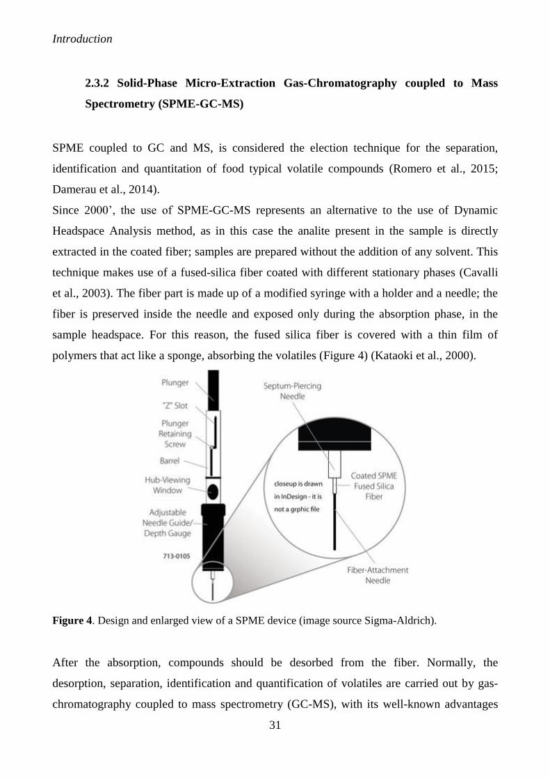
Introduction
31
2.3.2 Solid-Phase Micro-Extraction Gas-Chromatography coupled to Mass
Spectrometry (SPME-GC-MS)
SPME coupled to GC and MS, is considered the election technique for the separation,
identification and quantitation of food typical volatile compounds (Romero et al., 2015;
Damerau et al., 2014).
Since 2000’, the use of SPME-GC-MS represents an alternative to the use of Dynamic
Headspace Analysis method, as in this case the analite present in the sample is directly
extracted in the coated fiber; samples are prepared without the addition of any solvent. This
technique makes use of a fused-silica fiber coated with different stationary phases (Cavalli
et al., 2003). The fiber part is made up of a modified syringe with a holder and a needle; the
fiber is preserved inside the needle and exposed only during the absorption phase, in the
sample headspace. For this reason, the fused silica fiber is covered with a thin film of
polymers that act like a sponge, absorbing the volatiles (Figure 4) (Kataoki et al., 2000).
Figure 4. Design and enlarged view of a SPME device (image source Sigma-Aldrich).
After the absorption, compounds should be desorbed from the fiber. Normally, the
desorption, separation, identification and quantification of volatiles are carried out by gas-
chromatography coupled to mass spectrometry (GC-MS), with its well-known advantages
Introduction
32
as an efficient tool for analyses of volatile and semi volatile compounds. After a suitable
extraction time, the fiber is reinserted inside the needle and subsequently placed in a GC
injection port; then the analytes are desorbed in the injector by heating. The sample solution
is injected into the GC inlet where it is vaporized and swept onto a chromatographic column
by the carrier gas (usually helium). The sample flows through the column and the
compounds comprising the mixture of interest are separated by virtue of their relative
interaction with the coating of the column (stationary phase) and the carrier gas (mobile
phase, usually helium). The final part of the column passes through a heated transfer line
and ends at the entrance to ion source where compounds eluting from the column are
converted to ions by electron ionisation (EI): a beam of electrons ionise the sample
molecules resulting in the loss of one electron. A molecule with one electron missing is
called the molecular ion and is represented by M+.(radical cation). The next component is a
mass analyser, which separates the positively charged ions according to various mass
related properties depending upon the analyser used. Several types of analyzers exist:
quadrupoles, ion traps, magnetic sector, time-of-flight, radio frequency, cyclotron resonance
and focusing to name a few. The most common are quadrupoles and ion traps. After the ions
are separated they enter a detector, the output from which is amplified to boost the signal.
When the resulting peak from this ion is seen in a mass spectrum, it gives the molecular
weight of the compound. Due to the large amount of energy imparted to the molecular ion it
usually fragments producing further smaller ions with characteristic relative abundances that
provide a 'fingerprint' for that molecular structure. This information may be then used to
identify compounds of interest and help elucidate the structure of unknown components of
mixtures (Figure 5). The detector sends information to a computer that records all the data
produced, converts the electrical impulses into visual displays and hard copy displays. In
addition, the computer also controls the operation of the mass spectrometer.
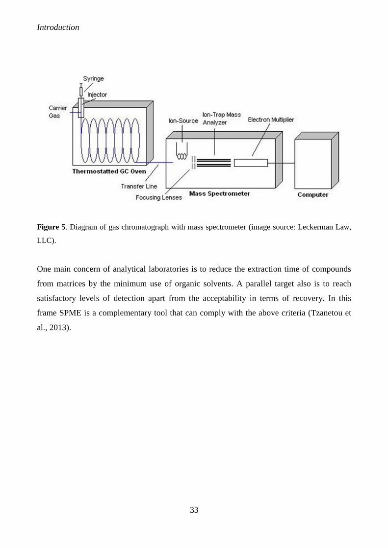
Introduction
33
Figure 5. Diagram of gas chromatograph with mass spectrometer (image source: Leckerman Law,
LLC).
One main concern of analytical laboratories is to reduce the extraction time of compounds
from matrices by the minimum use of organic solvents. A parallel target also is to reach
satisfactory levels of detection apart from the acceptability in terms of recovery. In this
frame SPME is a complementary tool that can comply with the above criteria (Tzanetou et
al., 2013).
Introduction
34
2.3.3 Odour detection methods: olfactometry and chemical sensors
An odour is a mixture of light and small molecules, also at very low concentrations in the
inhaled air, which, upon coming in contact with the human sensory system, is able to
stimulate an anatomical response: the experienced perception is the odour (Craven et al.,
1996).
Among the most innovative methods for the analysis of volatile compounds the application
of so-called "electronic noses" (E-noses) can be mentioned, as a system developed with the
aim to mimic the human olfaction in the discrimination of odors (Röck et al., 2008).
The discovery of materials with chemo-electronic properties has provided the opportunity
for the development of artificial olfactory instruments mimicking the biological system
(Craven et al., 1996). In the last ten years, a large field of scientific research has been
devoted to the development of E-Nose that are sensor-based instruments, capable of
discrimination between a variety of simple and complex odours.
Instrumental approaches to the characterization of odorants are based on the evaluation of
the air chemical composition. First, the odorous air needs to be collected for subsequent
analysis: the traditional volatile organic compounds (VOCs) sampling methods, like
adsorbers or metal canister and polymer bags. According to the principle of the system used,
electronic noses can be divided in different generations.
2.3.3a Sensor-based electronic noses
The first generation of electronic noses was constituted by metal oxide sensors with
different selectivity; these sensors send electrical signals in the presence of volatile
molecules (Ragazzo-Sanchez et al., 2005). The main advantage of this method is
represented by the rapid identification of the sample smell, without the necessity of
identifying every single compound responsible for the smell itself (Xia et al., 2015; Wilson
et al., 2009). Several studies, related to the application of electronic nose to different food
matrices, have already been published (Messina et al., 2015; Cimato et al., 2006; Cosio et
al., 2006a; Cosio et al., 2006b). Like human olfaction, E-Noses are based on “an array of
electronic-chemical sensors with partial specificity to a wide range of odorants and an
appropriate pattern recognition system” (Gardner et al., 1994). In contrast to the ideal gas
sensors, which are required to be highly specific to a single chemical species, sensors for E-
Introduction
35
Nose need to give broadly tuned responses like the olfactory receptors in the human nose: in
both cases the odour quality information and recognition is ensured by the entire pattern of
responses across the sensors array, rather than the response of any one particular sensor.
Furthermore, mimicking the data processing in the biological systems, the incoming chemo-
electronic signals are processed through the use of data reduction techniques (Principal
Component Analysis - PCA); in both human and electronic noses, the function of odour
recognition is finally achieved by means of some form of associative memory for the
storage and recall of the previously encountered odours.
A wide variety of competing sensor technologies (conducting polymers, piezoelectric
devices, electrochemical cells, metal oxide sensors (MOX) and metal-insulator
semiconductor field effect transistors (MISFETs)) are currently available: independently of
the considered device, sensor elements have to show fast, reproducible and reversible
responses to odour samples (Ampuero et al., 2003; Pearce, 1997).
Chemical sensors comprise an appropriate and chemically-sensitive material interfaced to a
transducer; hence, the solid-state sensors are essentially constituted by a chemically
sensitive interface (sensitive material) and a transducer able to convert a chemical input (gas
concentration or ions concentration) and/or physical input (temperature, pressure,
acceleration, etc.) into an output, generally an electrical signal, by means of a conditioning
and/or signal processing electronics. The input magnitudes include chemical and/or
biological magnitudes such as concentration and identity of unknown species in gaseous or
liquid phase, other than physical general magnitudes such as temperature, pressure, speed,
acceleration and force. A transduction process is realized by converting the input-event into
an output electrical signal (analogue voltage or current, digital voltage) correlated to the
measurand that generates it. The output electrical signal is properly conditioned, processed
and stored for analysis (Gardner et al., 1991). Gas sensors, based on the chemical sensitivity
of semiconducting metal oxides, are readily available commercially and have been more
widely used to make arrays for odour measurement than any other single class of gas
sensors. On the other hand, the various categories of solid-state chemical sensors are
differentiated by the physical principle of the signal transduction by distinguishing the
following transducers: conductometric (resistive), optical, electrochemical,
mechanical/acoustic or ultrasonic, thermal and MISFET.
Introduction
36
2.3.3b GC-based electronic noses
Dynamic olfactometry. As occurring in the industry (i.e., food, beverages, perfumes, etc.)
for many years, the sensory evaluation of smells by means of panels of sensory trained
evaluators has been the main odour assessment and quantification tool: the so-called
dynamic olfactometry is the standardized method used for determining the concentration of
odours and evaluating odour complaints (Schulz et al., 1996).
This methodology is based on the use of a dilution instrument, called olfactometer, which
presents the odour sample diluted with odour-free air at precise ratios, to a panel of human
assessors. The examiners are selected in compliance with a standardized procedure
performed using reference gases; only assessors who meet predetermined repeatability and
accuracy criteria are selected as panelists. The odour concentration, usually expressed in
odour units (ou/m3) is numerically equal to the dilution factor necessary to reach the odour
threshold, that is the minimum concentration perceived by 50% of population (EN13725).
According to European standardization, 1 ou/m3 is defined as the amount of odourant that,
when evaporated into 1 m3 of gas air at standard conditions, causes a physiological response
from a panel (detection threshold) equivalent to that of n-butanol (reference gas) evaporated
into 1 m3 of neutral gas. The perception of odours is a logarithmic phenomenon (Stevens,
1960); for this reason, in this kind of measurements it is necessary taking into account that
odour concentration is associated to odour intensity though a defined logarithmic relation.
The opportunity of using sensory perception for the development of conventional
instruments for chemical analysis is represented by gas chromatography-olfactometry (GC-
O) technique that couples the traditional gas chromatographic analysis with sensory
detection, in order to study complex mixtures of odorous compounds (Leland et al., 2001).
The gas chromatographic separation of an odorous air sample could be useful for
identifying specific odorant components: GC-O, thus, allows a deeper comprehension of the
odorant composition as concerns the compounds’ identification and quantification, offering
the advantage of a partial correlation between the odorant chemical nature and the perceived
smell (Friedrich et al., 1998). The schematic representation of a GC-O equipment is
reported in Figure 6.
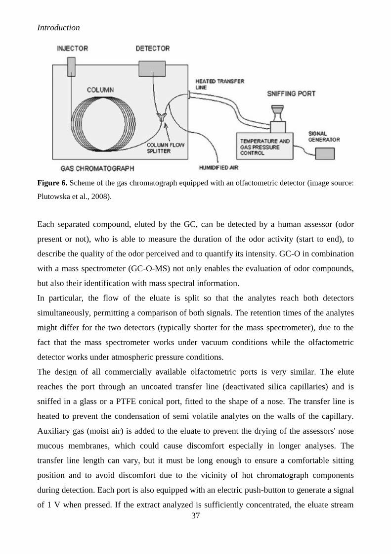
Introduction
37
Figure 6. Scheme of the gas chromatograph equipped with an olfactometric detector (image source:
Plutowska et al., 2008).
Each separated compound, eluted by the GC, can be detected by a human assessor (odor
present or not), who is able to measure the duration of the odor activity (start to end), to
describe the quality of the odor perceived and to quantify its intensity. GC-O in combination
with a mass spectrometer (GC-O-MS) not only enables the evaluation of odor compounds,
but also their identification with mass spectral information.
In particular, the flow of the eluate is split so that the analytes reach both detectors
simultaneously, permitting a comparison of both signals. The retention times of the analytes
might differ for the two detectors (typically shorter for the mass spectrometer), due to the
fact that the mass spectrometer works under vacuum conditions while the olfactometric
detector works under atmospheric pressure conditions.
The design of all commercially available olfactometric ports is very similar. The elute
reaches the port through an uncoated transfer line (deactivated silica capillaries) and is
sniffed in a glass or a PTFE conical port, fitted to the shape of a nose. The transfer line is
heated to prevent the condensation of semi volatile analytes on the walls of the capillary.
Auxiliary gas (moist air) is added to the eluate to prevent the drying of the assessors' nose
mucous membranes, which could cause discomfort especially in longer analyses. The
transfer line length can vary, but it must be long enough to ensure a comfortable sitting
position and to avoid discomfort due to the vicinity of hot chromatograph components
during detection. Each port is also equipped with an electric push-button to generate a signal
of 1 V when pressed. If the extract analyzed is sufficiently concentrated, the eluate stream
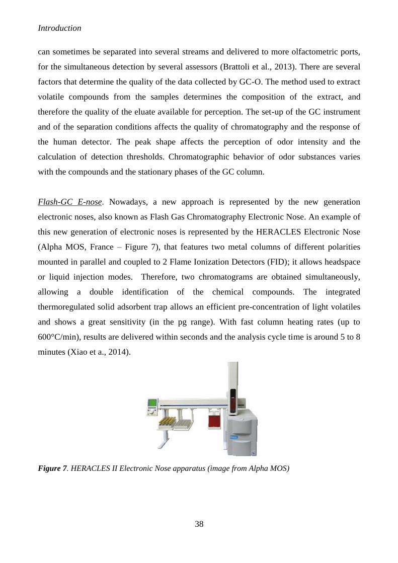
Introduction
38
can sometimes be separated into several streams and delivered to more olfactometric ports,
for the simultaneous detection by several assessors (Brattoli et al., 2013). There are several
factors that determine the quality of the data collected by GC-O. The method used to extract
volatile compounds from the samples determines the composition of the extract, and
therefore the quality of the eluate available for perception. The set-up of the GC instrument
and of the separation conditions affects the quality of chromatography and the response of
the human detector. The peak shape affects the perception of odor intensity and the
calculation of detection thresholds. Chromatographic behavior of odor substances varies
with the compounds and the stationary phases of the GC column.
Flash-GC E-nose. Nowadays, a new approach is represented by the new generation
electronic noses, also known as Flash Gas Chromatography Electronic Nose. An example of
this new generation of electronic noses is represented by the HERACLES Electronic Nose
(Alpha MOS, France – Figure 7), that features two metal columns of different polarities
mounted in parallel and coupled to 2 Flame Ionization Detectors (FID); it allows headspace
or liquid injection modes. Therefore, two chromatograms are obtained simultaneously,
allowing a double identification of the chemical compounds. The integrated
thermoregulated solid adsorbent trap allows an efficient pre-concentration of light volatiles
and shows a great sensitivity (in the pg range). With fast column heating rates (up to
600°C/min), results are delivered within seconds and the analysis cycle time is around 5 to 8
minutes (Xiao et a., 2014).
Figure 7. HERACLES II Electronic Nose apparatus (image from Alpha MOS)
Introduction
39
The sofware for the instrument management and control can also perform multivariate
statistical analysis as Principal Component Analysis (PCA), Partial Least Square (PLS),
Discriminant Factor Analysis (DFA), Statistical Quality Control (SQC) and Soft
Independent Modelling of Class Analysis (SIMCA). The compounds are detected using FID
detector and the software is able to “tag” every single molecule by comparison of its Kovats
retention index saved in the database of the instrument. Several studies regarding the use on
new generation electronic noses have been already published, concerning different food
matrices as: virgin olive oil with different geographical origin (Melucci et al., 2016), plum
and cherry spirits differently produced and with different geographical origin (Śliwińska et
al., 2016a and 2016b), meat produced with porks differently feeded (Wojtasik-Kalinowska
et al., 2016), slimming pills produced with the addition of prohibited substances (Xia et al.,
2015), sorgum distilled with different geographical origin (Peng et al., 2015), odour
nuisance from landfill (Gębicki et al., 2014), quality evaluation of agricultural distillates
(Dymerski et al., 2014).
2.4 Data Analysis
All measurements were carried out in triplicate (if not stated otherwise), and the results are
expressed as mean values (± standard deviations). The analysis of variance and multivariate
analysis of data were perfomed with XLSTAT version 2011.1.03 software, when other
statistical softwares were used, they are specified in the following sections. In the first
study, PCA, partial Least Square analysis and pairwise t-test were used for the evaluation of
volatile compounds data. Statistical analysis of sensory data was carried out calculating
median values. In the second study, the significant differences in terms of chemical
compounds amounts were calculated with Fisher Least Significant Differences (Fisher LSD)
and a value of p ≤ 0.05 was considered to be statistically significant. In the third study, the
peak areas were area normalized and mean centred before the PCA and SPME-GC-MS data
were explored with ANOVA and subsequently with PCA (IBM – SPSS) and combined to
sensory mean values by means of multifactorial analysis (MFA). The significant differences
in terms of chemical compounds amounts were calculated with Fisher Least Significant
Differences (Fisher LSD) and a value of p ≤ 0.05 was considered to be statistically
significant. In the fourth study, peak areas were area normalized and mean centred before
the PCA and SPME-GC-MS. The analysis of variance was carried out and data were
Introduction
40
analysed with PCA; sensory, chemical and instrumental (analysis of image and textural
properties) data were combined with MFA. In the fifth study, data from sensory and
instrumental (analysis of image and textural properties) analysis were explored with PCA
with Unscrambler® X (v.10.1; CAMO Software AS, 2011, Norway). The precision and the
predictive capabilities of the models were evaluated by the coefficients of determination
(R2) and root-mean square error estimated by cross-validation (RMSECV). In the last study,
preference data were analysed according to chi square test (p>0.05). Statistical analysis of
data was carried out using the SAS/STAT statistical software package version 9.3.1. (SAS
Institute Inc., Cary, USA).
Introduction
41
2.5 References
Ampuero S., Bosset J.O. 2003. The electronic nose applied to dairy products: a review.
Sensors and Actuators B: Chemical, 94, 1-12.
Angerosa F., Servili M., Selvaggini R., Taticchi A., Esposto S., Montedoro G. 2004. Volatile
compounds in virgin olive oil: occurrence and their relationship with the quality. Journal of
Chromatography A, 1054, 17-31.
Angerosa F. 2002. Influence of volatile compounds on virgin olive oil quality evaluated by
analytical approaches and sensor panels. European Journal of Lipid Science and
Technology, 104, 639-660.
Bárcenas P., Elortondo F.P., Albisu M. 2000. Selection and screening of a descriptive panel
for ewes milk cheese sensory profiling. Journal of Sensory Studies, 15, 79-99.
Bianchi F., Cantoni C., Careri M., Chiesa L., Musci M., Pinna A. 2007. Characterization of
the aromatic profile for the authentication and differentiation of typical Italian dry-sausages.
Talanta, 72, 1552-1563.
Bicchi C., Cordero C., Iori C., Rubiolo P., Sandra P. 2000. Headspace sorptive extraction
(HSSE) in the headspace analysis of aromatic and medicinal plants. Journal of Separation
Science, 23, 539-546.
Brattoli M., Cisternino E., Dambruoso P.R., de Gennaro G., Giungato P., Mazzone A.,
Palmisani J., Tutino M. 2013. Gas chromatography analysis with olfactometric detection
(GC-O) as a useful methodology for chemical characterization of odorous compounds.
Sensors, 13, 16759-16800.
Brattoli M., De Gennaro G., De Pinto V., Demarinis Loiotile A., Lovascio S., Penza M. 2011.
Odour detection methods: Olfactometry and chemical sensors. Sensors, 11, 5290-5322.
Carpenter R. P., Lyon D. H., Hasdell T. A. 2012. Guidelines for sensory analysis in food
product development and quality control. Springer Science & Business Media.
Caul J.F. 1957. The profile method of flavor analysis. Advances in food research, 7, 1-40.
Cavalli J.F., Fernandez X., Lizzani-Cuvelier L., Loiseau A.M. 2003. Comparison of static
headspace, headspace solid phase microextraction, headspace sorptive extraction, and direct
thermal desorption techniques on chemical composition of French olive oils. Journal of
Agricultural and Food Chemistry, 51, 7709-7716.
Introduction
42
Cimato A., Dello D., Distante C., Epifani M., Siciliano A., Taurino M., Zuppa M., Sani G.
2006. Analysis of single-cultivar extra virgin olive oils by means of an electronic nose and
HS-SPME-GC-MS methods. Sensors and Actuators B, 114, 674-680.
Cosio M.S., Ballabio D., Benedetti S., Gigliotti C. 2006a. Evaluation of different storage
conditions of extra virgin olive oils with an innovative recognition tool built by means of
electronic nose and electronic tongue. Food Chemistry, 101, 485-491.
Cosio M.S., Ballabio D., Benedetti S., Gigliotti C. 2006b. Geographical origin and
authentication of extra virgin olive oils by an electronic nose in combination with artificial
neural network. Analytical Chimica Acta, 567, 202-210.
Craven M.A., Gardner J.W., Bartlett P.N. 1996. Electronic noses—development and future
prospects. TrAC Trends in Analytical Chemistry, 15, 486-493.
Crescitelli F. 1960. Physiology of vision. Annual review of physiology, 22, 525-578.
Da Conceicao Neta E.R., Johanningsmeier S.D., McFeeters R.F. 2007. The chemistry and
physiology of sour taste—a review. Journal of food science, 72, 33-38.
Damerau A., Kamlang-ek P., Moisio T., Lampi A.M., Piironen V. 2014. Effect of SPME
extraction conditions and humidity on the release of volatile lipid oxidation products from
spray-dried emulsions. Food Chemistry, 157, 1-9.
Delahunty C.M., Eyres G., Dufour J.P. 2006. Gas chromatography‐olfactometry. Journal of
Separation Science, 29, 2107-2125.
Dymerski T., Gębicki J., Namieśnik J. 2014. Comparison of quality evaluation of agricultural
distillates using prototype of Electronic Nose and Fast/Flash GC, 40, 127-132.
EN13725: Air Quality—Determination of Odour Concentration by Dynamic Olfactometry;
Committee for European Normalization (CEN), Brussels, Belgium, 2003.
Escuderos M.E., Uceda M., Sànchez S., Jìmenez A. 2007. Instrumental technique evolution
for olive oil sensory analysis. European Journal of Lipid Science and Technology, 109, 536-
546.
Friedrich J.E., Acree, T.E. 1998. Gas chromatography olfactometry (GC/O) of dairy
products. International Dairy Journal, 8, 235-241.
García-González D.L., Tena N., Aparicio R. 2009. Contributing to interpret sensory attributes
qualifying Iberian hams from the volatile profile. Grasas y Aceites, 60, 277-283.
Introduction
43
Gardner J.W., Bartlett P.N. 1991. Pattern recognition in gas sensing. Techniques and
Mechanisms in Gas Sensing, 374-380.
Gardner J.W., Bartlett P.N. 1994. A brief history of electronic noses. Sensors and Actuators
B: Chemical, 18, 210-211.
Gębicki J., Dymerski T., Namieśnik J. 2014. Monitoring of odour nuisance from landfill
using Electronic Nose. Chemical Engineering Transactions, 40, 85-90.
ISO standard 5492:2008. Sensory Analysis. Vocabulary.
Jones L.V., Peryam D.R., Thurstone L.L. 1955. Development of a scale for measuring
soldiers’food preferences. Journal of Food Science, 20, 512-520.
Kalua C.M., Allen M.S., Bedgood D.R., Bishop A.G., Prenzler P.D., Robards K. 2007. Olive
oil volatile compounds, flavour development and quality: A critical review. Food
Chemistry, 100, 273-286.
Kataoka H., Lord H.L., Pawliszyn J. 2000. Applications of solid-phase microextraction in
food analysis. Journal of Chromatography A, 880, 35-62.
Korsmeyer C. 2002. Making sense of taste: Food and philosophy. Cornell University Press.
Lawless, H.T., Heymann, H. 2010. Sensory evaluation of food: principles and practices.
Springer Science & Business Media.
Leland J.V., Schieberle P., Buettner A., Acree T.E. 2001. Gas chromatography-olfactometry:
the state of the art. American Chemical Society. Eds.
McNair H. M., Miller J. M. 2009. Introduction. In: Basic Gas Chromatography, 2nd ed. Eds.
McNair H. M. and Miller J. M., Hoboken (NJ).
Melucci D., Bendini A., Tesini F., Barbieri S., Zappi A., Vichi S., Conte L., Gallina Toschi
T. 2016. Rapid direct analysis to discriminate geographic origin of extra virgin olive oils by
flash gas chromatography electronic nose and chemometrics. Food Chemistry, 204, 263-
273.
Mentasti E., Saini G. 1990. Analisi chimica cromatografica. Piccin.
Messina V., Sancho A., Walsöe de Reca N. 2015. Monitoring odour of heated extra-virgin
olive oils from Arbequina and Manzanilla cultivars using an electronic nose. European
Journal of Lipid Science and Technology, 117, 1295-1300.
Introduction
44
Morales M.T., Aparicio-Ruiz R., Aparicio R. 2013. Chromatographic methodologies:
compounds for olive oil odor issues. In Handbook of Olive Oil (pp. 261-309). Springer US.
Morales MT., Aparicio R., Gutiérrez F. 1992. Técnicas de aislamiento y concentración de
volátiles de aceites vegetales. Grasas Aceites 43,164–173.
Moret S., Purcaro G., Conte L.S. 2014. Il campione per l’analisi chimica: Tecniche
innovative e applicazioni nei settori agroalimentare e ambientale. Springer.
Murray J.M., Delahunty C.M., Baxter I.A. 2001. Descriptive sensory analysis: past, present
and future. Food research international, 34, 461-471.
Nachtsheim R., Ludi R., Schlich E. 2012. Relationship between product specific and
unspecific screening tests and future performance of descriptive panellists. Eurosense
Meeting, Berne, Switzerland, September 9—12.
Noronha R.L., Damasio M.H., Pivatto M.M., Negrillo B.G. 1995. Development of the
attributes and panel screening for texture descriptive analysis of milk gels aided by
multivariate statistical procedures. Food Quality and Preference, 6, 49-54.
O'Sullivan M. 2016. A handbook for sensory and consumer-driven new product
development. Innovative technologies for the food and beverage industry. Woodhead
publishing.
Pagliarini E. 2002. Valutazione sensoriale: aspetti teorici, pratici e metodologici. Ulrico
Hoepli.
Pearce T.C. 1997. Computational parallels between the biological olfactory pathway and its
analogueThe Electronic Nose': Part II. Sensor-based machine olfaction. Biosystems, 41, 69-
90.
Pelosi P. 1985. Classificazione e misura degli odori. Caratteristiche olfattive e gustative degli
alimenti. Chiriotti, Torino.
Peng Q., Tian R., Chen F., Li B., Gao H. 2015. Discrimination of producing area of Chinese
Tongshan kaoliang spirit using electronic nose sensing characteristics combined with the
chemometrics methods. Food Chemistry, 178, 301-305.
Peryam D.R., Swartz V.W. 1950. Measurement of sensory differences. Food Technology, 4,
390-395.
Introduction
45
Plutowska B., Wardencki W. 2008. Application of gas chromatography–olfactometry (GC–
O) in analysis and quality assessment of alcoholic beverages–A review. Food chemistry,
107, 449-463.
Qian M. C. 2010. Gas chromatography. In: Food Analysis. Ed. Nielsen. New York, Springer.
Ragazzo-Sanchez J.A., Chalier P., Ghommidh C. 2005. Coupling gas chromatography and
electronic nose for dehydration and desalcoholization of alcoholized beverages: Application
to off-flavour detection in wine. Sensors and Actuators B: Chemical, 106, 253-257.
Röck F., Barsan N., Weimar U. 2008. Electronic nose: current status and future trends.
Chemical Reviews, 108, 705-725.
Romero I., García-González D.L., Aparicio-Ruiz R., Morales M.T. 2015. Validation of
SPME–GCMS method for the analysis of virgin olive oil volatiles responsible for sensory
defects. Talanta, 134, 394-401.
Roper S.D. 2007. Signal transduction and information processing in mammalian taste buds.
Pflügers Archiv-European Journal of Physiology, 454, 759-776.
Rozin P. 1982. “Taste-smell confusions” and the duality of the olfactory sense. Attention,
Perception, & Psychophysics, 31, 397-401.
Schulz T.J., Van Harreveld A. P. 1996. International moves towards standardisation of odour
measurement using olfactometry. Water Science and Technology, 34, 541-547.
Śliwińska M., Wiśniewska P., Dymerski T., Wardencki W., Namieśnik J. 2016a. Evaluation
of the suitability of electronic nose based on fast GC for distinguishing between the plum
spirits of different geographical origins. European Food and Research Technology.
Śliwińska M., Wiśniewska P., Dymerski T., Wardencki W., Namieśnik J. 2016b. Application
of Electronic Nose based on Fast GC for authenticity assessment of Polish homemade
liqueurs called Nalewka. Food Analytical Methods, 9, 2670-2681.
Stevens S.S. 1960. The psychophysics of sensory function. American Scientist, 48, 226-253.
Stone H., Bleibaum R., Thomas H.A. 2012. Sensory evaluation practices. Academic press.
Szczesniak A.S. 2002. Texture is a sensory property. Food quality and preference, 13, 215-
225.
Van Gemert L.J. 2003. Odour thresholds. Compilations of odour threshold values in air,
water and other media. Utrecht (The Netherlands): Oliemans Punter & Partners BV.
Introduction
46
Varela P., Ares G. 2012. Sensory profiling, the blurred line between sensory and consumer
science. A review of novel methods for product characterization. Food Research
International, 48, 893-908.
Varela P., Ares G. 2014. Novel techniques in sensory characterization and consumer
profiling. CRC Press.
Vichi S. 2010. Extraction techniques for the analysis of virgin olive oil aroma in “Olives and
olive oil in health and disease prevention”, Academic Press Editor, 615-623.
Vickers Z. 1991. Sound perception and food quality. Journal of Food Quality, 14, 87-96.
Wilson A.D., Baietto M. 2009. Applications and advances in electronic-nose technologies.
Sensors, 9, 5099-5148.
Wojtasik-Kalinowska I., Guzek D., Górska-Horczyczak E., Głąbska D., Brodowska M., Sun
D., Wierzbicka A. 2016. Volatile compounds and fatty acids profile in Longissimus dorsi
muscle from pigs fed with feed containing bioactive components. LWT-Food Science and
Technology, 67, 112-117.
Xia Z., Cai W., Shao X. 2015. Rapid discrimination of slimming capsules based on illegal
additives by electronic nose and flash gas chromatography. Journal of Separation Science,
38, 621-625.
Xiao Z., Yu D., Niu, Y., Chen F., Song S., Zhu J., Zhu G. 2014. Characterization of aroma
compounds of Chinese famous liquors by gas chromatography–mass spectrometry and flash
GC electronic-nose. Journal of Chromatography B, 945, 92-100.
Results
47
3. Results
3.1 Rapid direct analysis to discriminate geographic origin of extra virgin olive oils by
flash gas chromatography electronic nose, sensory analysis and chemometrics
Publication details:
Original title: Rapid direct analysis to discriminate geographic origin of extra virgin olive oils by
flash gas chromatography electronic nose, sensory analysis and chemometrics
Authors: Melucci Da, Bendini Ab, Tesini Fb, Barbieri Sb, Zappi Aa, Vichi Sc, Conte LSd, Gallina
Toschi Tb a Department of Chemistry Ciamician, University of Bologna, Via Selmi, 2, 40126 Bologna, Italy b Department of Agricultural and Food Sciences (DiSTAL), University of Bologna, P.zza
Goidanich 60, 47521 Cesena, Italy c Department of Food Science and Nutrition, University of Barcelona, Food and Nutrition Torribera
Campus, Av. Prat de la Riba, 171, S.ta Coloma de Gramenet, Spain d Department of Food Science, University of Udine, Via Sondrio 2/a, 33100 Udine, Italy
Published on: Food Chemistry. 2016. 204, 263-273.
3.1.1 Abstract
At present, the geographical origin of extra virgin olive oils can be ensured by documented
traceability, although chemical analysis may add information that is useful for possible
confirmation. This preliminary study investigated the effectiveness of flash gas
chromatography electronic nose and multivariate data analysis to perform rapid screening of
commercial extra virgin olive oils characterized by a different geographical origin declared
in the label. A comparison with solid phase micro extraction coupled to gas chromatography
mass spectrometry was also performed. The new method is suitable to verify the geographic
origin of extra virgin olive oils based on principal components analysis and discriminant
analysis applied to the volatile profile of the headspace as a fingerprint. The selected
variables were suitable in discriminating between ‘‘100% Italian” and ‘‘non-100% Italian”
oils. Partial least squares discriminant analysis also allowed prediction of the degree of
membership of unknown samples to the classes examined.
Keywords: Extra virgin olive oil; Geographic origin; FGC E-nose; SPME-GC–MS;
Headspace volatile compounds; Non-target analysis; PCA; PLS-DA.
Results
48
3.1.2 Introduction
In an increasingly globalized world, certification of food quality is one of the most
important goals for scientists in the agri-food sector. Consumer demand of traceability and
authenticity of food products is also increasing, and the international agencies dealing with
food quality have recently published specific guidelines in this regard (FAO, 2003). Extra
virgin olive oil (EVOO) is a typical Mediterranean food product characterized by a multi-
millenary tradition that arouses great appreciation among consumers. Within the
Mediterranean basin, Italy is a key producer of olive oil. The vast economic interests may
give rise to illegal activities aimed to increase profit, such as a false declaration of
geographic origin, thus falsifying traceability and, consequently, authenticity of the product.
The European Union (EU) has recently concluded a decennial iter to establish regulations
about olive oil with the aim of regulating production and commercialization of this
important product. Regulation EU No. 1019/02 defined how to correctly pack and label oils,
and the last Commission Implementing Regulation, 2013 EU No. 1335/13 made it
obligatory to indicate the geographic origin on the label. In EU Regulation No. 29/12
(European Commission Implementing Regulation, 2012), it is reported that in order to
ensure that consumers are not misled and the olive oil market is not distraught, information
concerning the geographic area in which olives are harvested and olive oil is obtained
should be stated on the packaging or labels. For greater clarification, the document also
defines that simple provisions as ‘blend of olive oils of European Union origin’ or ‘blend of
olive oils not of European Union origin’ or ‘blend of olive oils of European Union origin
and not of European Union origin’ should be stated for labeling of origin. The mandatory
necessity of certifying the geographical origin makes it highly desirable to assess origin not
only by documentation of verification, but also by rapid analytical methods. In this regard, it
is necessary to apply high performance instrumental analytical methods, and the large
number of variables imposes the use of chemometrics, whose outputs provide useful and
easy-to visualize information extracted from data while simultaneously discarding useless
information (analytical noise and redundant information). There is an urgent need to extend
the representativeness of a database established on chromatographic, spectroscopic, and
spectrometric compositional data profiles to clearly identify the most promising techniques
in order to confirm the geographic origin of EVOOs and verify the conformity of label-
Results
49
declared geographic origin, as well as to provide one or more harmonized methods for
sharing markers that are useful to check the product’s conformity to specific standards (e.g.,
geographical origin). All the factors identified by compositional analysis of EVOOs are
important. Mass spectrometry together with various spectrometric and chromatographic
analytical techniques have been applied to determine the chemical composition, and many
of these instrumental analytical techniques have been used in tandem with chemometrics
(Gouvinhas, et al., 2015; Azizian et al., 2015; Mendes et al., 2015; Sinelli et al., 2010;
Diraman et al., 2009; Dibeklioǧlu, 2009). In this context, adulteration of EVOOs has been
studied by liquid chromatography (HPLC), GC, and linear discriminant analysis (LDA)
using fatty acids (FA) and triacylglycerols (TGs) as markers (Jabeur et al., 2014; Ollivier et
al., 2006). HPLC-mass spectrometry (MS) and LDA allowed determination of the phenolic
profile for discrimination of geographical origin (Taamalli et al., 2012). In particular,
specific volatile compounds or their classes (e.g., terpenoid compounds) have been used to
discriminate EVOO samples according to geographic origin (Cecchi et al., 2013; Ben
Temime et al., 2006; Zuninet al., 2005; Vichi et al., 2003). Many EVOOs have also been
classified according to their geographic origin using the combination of FA and/or TG
profiles with other compounds such as sterols, polyphenols, and volatiles using
conventional and new analytical approaches, as recently reviewed (Gallina Toschi et al.,
2013; García-González et al., 2009). Several publications have described the use of volatile-
species distribution as a fingerprint to assess traceability, authentication, and non-
degradation based on head-space sampling and GC in tandem with several chemometric
tools: analysis of variance (ANOVA) and correlation analysis (Cecchi et al., 2013);
principal components analysis (PCA) (Cimato et al., 2006); LDA (Pouliarekou et al., 2011);
PCA and hierarchical clustering analysis (HCA) (Procida et al., 2005). Among the chemical
species in EVOO, many volatiles have been related with specific sensory characteristics
(Aparicio et al., 2008). Over the last decade, ‘‘e-sensing” technologies have undergone
important developments from a technical and commercial point of view, and electronic
noses have been designed to mimic the human sense of olfaction in order to detect and
recognize flavors and off-flavors in different food matrices (Peng et al., 2015). Moreover,
the electronic nose results have been successfully correlated to those obtained with other
techniques (sensory, GC, and GC–MS) (Lerma- García et al., 2010; Mildner-Szkudlarz et
Results
50
al., 2008). In a traditional multivariate approach, the variables are concentrations of several
compounds: this means that the scientist chooses beforehand which chemical species are
relevant; in contrast, when tools like PCA or partial least squares discriminant analysis
(PLS-DA) are applied to full chromatograms, there is no risk to discard species with
retention times not corresponding to chemical species already known to influence EVOO
quality. The advantages of such an approach have recently been described (Melucci et al.,
2013). The aim of this study was to analyze the headspace profile of commercial EVOOs
with different geographic origin using electronic nose with flash gas chromatography (FGC
E-nose), which is able to perform the separation on two short columns of different polarities
working in parallel and detect analytes with a flame ionization detector (FID). The FGC E-
nose was used to discriminate between products labeled as ‘‘100% Italian EVOO” and
‘‘non-100% Italian” coming from other countries in the EU, and in particular Spain and
Greece. PCA, LDA, and HCA were applied as exploratory tools. Data processing was
initially applied to datasets made from peak areas at retention times corresponding to
significant species; in this case, a comparison between the non-target analysis performed by
FGC E-nose and SPME-GC–MS achieved two purposes: (i) to demonstrate that the
discriminating power of FGC E-nose was comparable with SPME-GC–MS; (ii) to assign
FGC E-nose retention times to specific volatile compounds. In a second step, the full
chromatograms, obtained on two different sets of samples analyzed in two different
laboratories, were processed by applying PLS-DA as a chemometric tool.
Results
51
3.1.3 Materials and Methods
3.1.3a Samples
The two sets of samples named Set A and Set B were formed by 27 and 251 EVOOs,
respectively, and were collected from COOP Italia before distribution by the supermarket
chain (COOP Italia is a consortium that acts as a central retailer and is one of the most
important supermarket chains in Italy; it also carries out marketing activities and performs
quality control). Set A was composed of 5 PDO (Protected Designation of Origin) and PGI
(Protected Geographical Indication) Italian samples, 13 samples declared as produced and
processed exclusively in Italy (100% Italian, I code), and 9 samples produced in countries
which are members of the European Union (Mixtures, M code). All samples in Set A were
collected during the 2012–2013 harvest period. Set B included 132 samples labeled as 100%
Italian (I) and 119 samples labeled as non-100% Italian (M) EVOOs collected during the
2013–2014 harvest period. Even if the actual identity of the samples was confidential, all
the olive oils were bottled (in dark or transparent glass bottles) in Italy. Moreover, samples
considered as 100% Italian were assumed to be as declared, according to specific quality
control checks, and based on chemometric control with single class PCA models and
Hotelling analysis for outliers elimination applied to confirm the geographic class. All
samples were stored at 10 °C in darkness before analysis.
3.1.3b Volatile compounds analysis
Flash Gas Chromatography Electronic Nose. The same type of FGC E-nose Heracles II
(AlphaMos, Toulouse, France) was used for both sets of samples but in two different
laboratories (Set A was analyzed in Toulouse, Set B in the laboratory of COOP Italia in
Bologna, Italy). The Heracles II was equipped with two columns working in parallel mode:
a non-polar column (MXT5: 5% diphenyl, 95% methylpolysiloxane, 10 m length and 180
µm diameter) and a slightly polar column (MXT1701: 14% cyanopropylphenyl, 86%
methylpolysiloxane, 10 m length and 180 µm diameter). A single comprehensive
chromatogram was created by joining the chromatograms obtained with the two columns;
such an approach may help in preventing/reducing incorrect identifications due to
overlapping of chromatograms obtained with two different columns, and represents a useful
Results
52
tool for improved identification. An aliquot of each sample (2 g ± 1%) was placed in a 20
mL vial and sealed with a magnetic plug. The vial was placed in the Heracles’ auto-sampler,
which placed it in a shaker oven where it remained for 20 min at 50 °C, shaken at 500 rpm.
Next, a syringe pierced the silicone septum of the magnetic plug and sampled 5 ml of the
head space. Prior to the chromatographic separation, the 5-ml headspace aliquot was
adsorbed on a CARBOWAX trap maintained at 40 °C for 65 s while the carrier gas (H2)
flowed through it in order to concentrate the analytes and to remove excess air and moisture.
Subsequently, desorption was obtained by increasing the temperature of the trap up to 240
°C in 93 s and the sample was injected. The thermal program started at 40 °C (held for 2 s)
and increased up to 270 °C at 3 °C s-1; the final temperature was held for 21 s. The total
separation time was 100 s. At the end of each column, a FID detector was placed and the
acquired signal was digitalized every 0.01 s. For calibration, an alkane solution (from n-
hexane to n-hexadecane) was used to convert retention time in Kovats indices and identify
the volatile compounds using specific software (AromaChemBase). Samples were analyzed
in triplicate or quadruplicate for both Set A and Set B.
SPME-GC-MS. The headspace composition was investigated by SPME coupled to GC
separation and MS detection. This same analysis was performed in two different
laboratories: samples in Set A were analysed at the University of Bologna (Italy), whereas
the laboratory of the University of Barcelona (Spain) performed analysis on Set B. The
same kind of instrument, a gas chromatograph Agilent 6890 N Network and a quadrupolar
mass-selective spectrometry Agilent 5973 Network detector (Agilent Technologies, Palo
Alto, CA, USA), provided with a split–splitless injection port and helium as the carrier gas
(linear velocity of 17 cm s-1) was used. Slight differences in analytical conditions were
applied. For analysis of Set A: SPME was carried out by weighing 1.5 g of sample, spiked
with 4-methyl-2-pentanone (internal standard dissolved in refined sunflower oil) to a
concentration of 10 mg kg-1 in a 10 mL vial fitted with a silicone septum. The vial was
placed in a water bath at 40 °C and maintaining the oil sample under magnetic stirring for 2
min (conditioning) and then a DVB/CAR/PDMS fiber (50/30 µm, 2 cm long from Supelco
Ltd., Bellefonte, PA) was exposed for 30 min in the headspace of the sample. After
exposition, the fiber was retracted into the needle and immediately desorbed for 3 min in the
Results
53
injection port of a gas chromatograph (250 °C). Compounds were separated on a ZB-WAX
column 30 m, 0.25 mm ID, 1.00 µm film thickness (Chemtek Analytic, Bologna, Italy).
Column temperature was held at 40 °C for 10 min and increased to 200 °C at 3 °C min-1.
The ion source and transfer line were at 180 °C and 230 °C, respectively. Electron impact
mass spectra were recorded at 70 eV ionization energy in the 20–250 amu mass range, 2
scans s-1. For analysis of Set B, SPME extraction was performed according to Vichi et al.
(2003) and differed from the method applied for Set A only for the use of a different
internal standard, 4-methyl-2-pentanol (Sigma–Aldrich, St. Louis, MO). The fiber was then
desorbed at 260 °C in the gas chromatograph injection port for 5 min. Separation of
compounds was performed on two columns with distinct polarity: Supelcowax-10 and
Equity-5 (both 30 m x0.25 mm I.D., 0.25 µm film thickness), both purchased from Supelco
(Supelco Ltd., Bellefonte, PA, USA). The column temperature was held at 40 °C for 5 min
and increased to 200 °C at 4 °C min-1. The injector temperature was 260 °C, and the transfer
line temperature was 280 °C. Electron impact mass spectra were recorded at 70 eV
ionization energy in the 30–300 amu mass range, 2 scans s-1. Identification of volatile
compounds was mainly carried out by a comparison of mass spectral data with information
from the National Institute of Standards and Technology (NIST) library (2005 version) and
checked with pure standards. Linear retention indexes were also calculated and compared
with those available in the literature. Relative amounts of volatile compounds were
expressed as mg of internal standard per kg of oil, applying a response factor of 1. All
determinations were carried out in triplicate or duplicate for Set A and Set B, respectively.
Results
54
3.1.3c Sensory analysis
A IOC panel test method was carried out on samples in Set A by a group of 8 selected
trained assessors, all members of the Professional Committee DiSTAL. Sample evaluation
was performed according to the official procedure (Reg. (EC) 640/2008). Moreover, the
presence of green notes and other positive attributes were evaluated with reference to the list
of descriptors for PDO EVOOs developed and agreed by the International Olive Oil
Council, 2005 (IOOC/T.20/Doc. No. 22, 2005).
3.1.3d Software
The FGC E-nose data processing was carried out with Alphasoft V12.44 and AroChembase
software. XLSTAT version 2011.1.03 software (Addinsoft, USA) was used to elaborate
ANOVA and PCA on Set A. Preliminary PCA on Set B and PLS-DA were performed using
The Unscrambler version 9.8 (CAMO, Norway).
3.1.3e Chemometrics
In this work, a first explorative step was carried out using peak areas that were
automatically calculated by the software that controls each instrument. All data based on
peak area were preprocessed by autoscaling. Principal component analysis is a well-known
chemometric procedure which rotates the original space to another one whose versors are
the principal components (PCs) oriented along directions containing the maximum
explained variance (EV) and mutually orthogonal. Score and loadings plots are obtained,
allowing for easy visualization of samples and variables and verification of their role in the
analytical problem. Hotelling analysis (HCA), applied to PCA scores, calculates the
covariance ellipsoid corresponding to 95% confidence level (and visually draws it on the
scores plot); therefore, samples falling outside of the ellipsoid are those in the multivariate
Gaussian tails and may be considered outliers and discarded from further analyses. Linear
discriminant analysis (LDA) is a multivariate classification tool which rotates the original
space, but unlike PCA its aim is to maximize separation between classes, minimizing at the
same time distances between objects in the same class; in this way, new objects may be
projected onto this new scores space and assigned to one of the classes of the training set.
Results
55
HCA may also be applied to identify eventual sub-classes by calculating multidimensional
Euclidean distances between objects and grouping those closest to each other. In the present
investigation, it was highly expected that various sub-categories may be included in the very
broad category ‘‘non-100% Italian” (M, for example mixtures from Spain, Greece, Italy).
Once the preliminary exploration by PCA, HCA, and LDA was completed, the work was
extended by creating models, or equations involving experimental variables. A very useful
response variable is the degree of belonging of objects to the possible classes involved in
the analytical problem. The main interest was in quantifying the degree of belonging to
class I (yI) and the degree of belonging to class M (yM). Few tens of objects are available
while up to thousands of variables (digitized signal) are generated by a FGC E-nose
chromatogram. Thus, the only adequate modeling tool is PLS regression (in particular, PLS-
DA), which exploits PCs and maximizes both EV and correlation between regressors (the
variables, that is the chromatographic signals at various retention times) and the response
(degree of belonging, y). The choice of using full chromatograms has important advantages:
(i) no preselection of significant retention times is needed, thus by-passing the non-target
character of FID signals; when no pre-selection is done, the risk of discarding useful
information is avoided; (ii) errors related to incorrect integration in peak-area calculation are
avoided. Of course, some disadvantages must also be considered when using whole
chromatograms as predictors: a number of correlated variables much higher than the number
of objects may lead to overfitting, which provides modeling noise instead of useful
information. However, chemometric modeling tools offer reliable methods for controlling
these problems to obtain good performance of PLS-regression, based on objective measures:
in particular, root mean square error (RMSE) and correlation coefficients. Predictive ability
(also for LDA) was evaluated by the well-known cross-validation (CV) procedure
(Brereton, 2007).
Results
56
3.1.4 Results and discussion
3.1.4a Explorative analysis of sample Sets A and B
The exploration of Set A was considered as a preliminary step in the method development
as it was the first to be analyzed and consequently taken into account to better define a
chemometric approach for discriminating such a large number of olive oil samples
subsequently studied. This first set of 27 samples was very useful for exploring Set B in
depth and in establishing the method.
3.1.4b PCA from SPME-GC-MS peak areas of Set A
According to the sensory analysis performed by IOC panel test method, the 27 samples of
Set A were classified as EVOO (8 samples) and VOO (19 samples); for EVOOs, the
intensity of fruity was light (4 samples) and medium (4 samples), and the presence of
secondary notes (olfactory and gustatory sensations) of almond, tomato, and grass was also
found. The VOOs showed several sensory defects, although “fusty/muddy” (off-flavor of
oils from olives stored in large amounts for many days before processing, or of oils left in
contact with the sediment for a long period of time, both leading to anaerobic fermentation)
was the most common. Other sensory defects found in VOO samples were rancid and
winey-vinegary. The volatile compounds identified and quantified in the headspace of the
analyzed samples by SPME-GC-MS are reported in Figure 1, which shows an overlap
between SPME-GC-MS traces relative to the profiles in volatiles molecules for M15
(mixture, non-100% Italian), I13 (100% Italian), and I23 (Italian PDO) samples. It is
interesting to note that the non-100% Italian sample (M15) showed a high content of C6
lipoxygenase (LOX) esters (hexylacetate and (Z)-3-hexenylacetate), which contribute to the
positive sensory notes of “sweet”, “fruity”, and “banana-like” (Kalua, et al., 2007) and, on
the other hand, a tendency towards a lower content in (E)-2-hexenal and (E)-2-hexenol, both
positively correlated with green sensory attributes such as “freshly cut grass”, “bitter
almond”, and “leaves”.
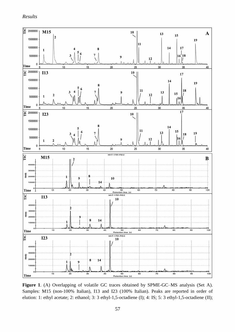
Results
57
Figure 1. (A) Overlapping of volatile GC traces obtained by SPME-GC–MS analysis (Set A).
Samples: M15 (non-100% Italian), I13 and I23 (100% Italian). Peaks are reported in order of
elution: 1: ethyl acetate; 2: ethanol; 3: 3 ethyl-1,5-octadiene (I); 4: IS; 5: 3 ethyl-1,5-octadiene (II);
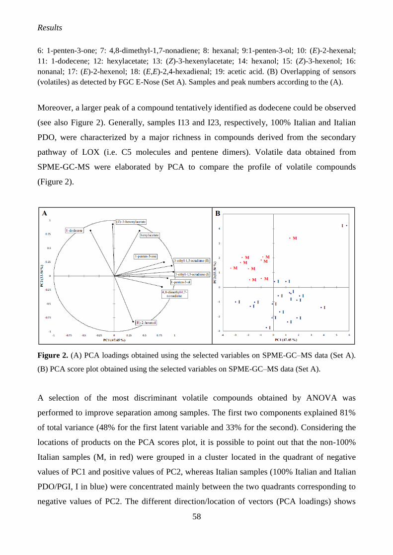
Results
58
6: 1-penten-3-one; 7: 4,8-dimethyl-1,7-nonadiene; 8: hexanal; 9:1-penten-3-ol; 10: (E)-2-hexenal;
11: 1-dodecene; 12: hexylacetate; 13: (Z)-3-hexenylacetate; 14: hexanol; 15: (Z)-3-hexenol; 16:
nonanal; 17: (E)-2-hexenol; 18: (E,E)-2,4-hexadienal; 19: acetic acid. (B) Overlapping of sensors
(volatiles) as detected by FGC E-Nose (Set A). Samples and peak numbers according to the (A).
Moreover, a larger peak of a compound tentatively identified as dodecene could be observed
(see also Figure 2). Generally, samples I13 and I23, respectively, 100% Italian and Italian
PDO, were characterized by a major richness in compounds derived from the secondary
pathway of LOX (i.e. C5 molecules and pentene dimers). Volatile data obtained from
SPME-GC-MS were elaborated by PCA to compare the profile of volatile compounds
(Figure 2).
Figure 2. (A) PCA loadings obtained using the selected variables on SPME-GC–MS data (Set A).
(B) PCA score plot obtained using the selected variables on SPME-GC–MS data (Set A).
A selection of the most discriminant volatile compounds obtained by ANOVA was
performed to improve separation among samples. The first two components explained 81%
of total variance (48% for the first latent variable and 33% for the second). Considering the
locations of products on the PCA scores plot, it is possible to point out that the non-100%
Italian samples (M, in red) were grouped in a cluster located in the quadrant of negative
values of PC1 and positive values of PC2, whereas Italian samples (100% Italian and Italian
PDO/PGI, I in blue) were concentrated mainly between the two quadrants corresponding to
negative values of PC2. The different direction/location of vectors (PCA loadings) shows
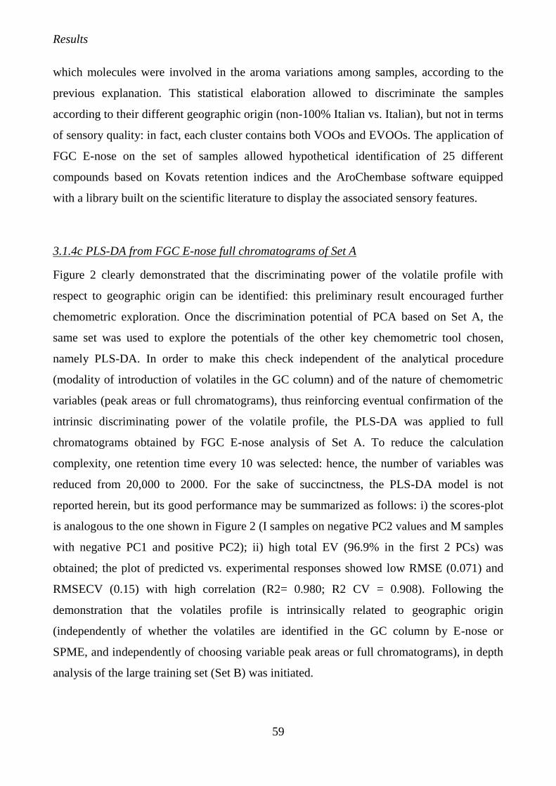
Results
59
which molecules were involved in the aroma variations among samples, according to the
previous explanation. This statistical elaboration allowed to discriminate the samples
according to their different geographic origin (non-100% Italian vs. Italian), but not in terms
of sensory quality: in fact, each cluster contains both VOOs and EVOOs. The application of
FGC E-nose on the set of samples allowed hypothetical identification of 25 different
compounds based on Kovats retention indices and the AroChembase software equipped
with a library built on the scientific literature to display the associated sensory features.
3.1.4c PLS-DA from FGC E-nose full chromatograms of Set A
Figure 2 clearly demonstrated that the discriminating power of the volatile profile with
respect to geographic origin can be identified: this preliminary result encouraged further
chemometric exploration. Once the discrimination potential of PCA based on Set A, the
same set was used to explore the potentials of the other key chemometric tool chosen,
namely PLS-DA. In order to make this check independent of the analytical procedure
(modality of introduction of volatiles in the GC column) and of the nature of chemometric
variables (peak areas or full chromatograms), thus reinforcing eventual confirmation of the
intrinsic discriminating power of the volatile profile, the PLS-DA was applied to full
chromatograms obtained by FGC E-nose analysis of Set A. To reduce the calculation
complexity, one retention time every 10 was selected: hence, the number of variables was
reduced from 20,000 to 2000. For the sake of succinctness, the PLS-DA model is not
reported herein, but its good performance may be summarized as follows: i) the scores-plot
is analogous to the one shown in Figure 2 (I samples on negative PC2 values and M samples
with negative PC1 and positive PC2); ii) high total EV (96.9% in the first 2 PCs) was
obtained; the plot of predicted vs. experimental responses showed low RMSE (0.071) and
RMSECV (0.15) with high correlation (R2= 0.980; R2 CV = 0.908). Following the
demonstration that the volatiles profile is intrinsically related to geographic origin
(independently of whether the volatiles are identified in the GC column by E-nose or
SPME, and independently of choosing variable peak areas or full chromatograms), in depth
analysis of the large training set (Set B) was initiated.
Results
60
3.1.4d PCA models based on FGC E-nose peak areas of Set B
Considering Set B, the training set to create chemometric models and the unknown set to
apply models must be extracted from all 251 EVOO samples that were analyzed in
quadruplicate by FGC E-nose. Each replicate corresponds to a row of the data set (object),
and thus 251 samples gave 1004 objects. In this first step of multivariate analysis of Set B,
the variables are the peak areas. Choosing the training set is a delicate step, because the
fidelity of the characteristics declared about the samples is crucial to the model’s
performance. In order to obtain a very reliable and consistent training set, the following
rationale was used. A PCA model was created from the 100% Italian samples, and Hotelling
analysis was performed. Only objects far inside the Hotelling ellipse were chosen; 224
objects were thus selected. The same was done with the M samples, and 269 objects were
selected. Therefore, the training set was formed of 493 objects. To verify the suitableness of
samples, a LDA scores plot (not reported) was created, and separation between classes was
excellent (94.2% correct assignments in cross validation). This is not an obvious result:
based on FGC E-nose areas, all Italian samples formed a homogeneous PCA cluster, and all
M samples constituted another homogeneous PCA cluster, but LDA showed that these two
clusters are separated, thus demonstrating the discriminating ability of FGC E-nose
variables and hence of the volatiles profile. This preliminary exploration allowed
identification of the 13 variables that were related to high discriminating power. In order to
explore eventual subgroups in M category (very wide in this case), a HCA was performed.
In fact, 3 clusters were observed in the M category, termed M1, M2, and M3 (dendrogram
not shown). The PCA analysis of these 493 selected objects obtained the results reported in
Figure 3. The resulting PCA model showed good performance since 81.3% EV was
obtained in calibration mode with only 6 PCs of 20 original variables. It can be seen that the
centroid of the I-cluster is far distant from the centroid of the M cluster. This is another
important proof of the suitability of the volatiles profile (here represented with FGC Enose
variables) to discriminate the geographic origin with respect to 100% Italian and non-100%
Italian EVOOs. However, several M2 samples in the scores plot in Figure 3 are near the I
centroid; this is not surprising, since a sample classified as “non-100% Italian” may contain
a fraction of Italian EVOO. The samples with the highest distance from the centroid were
Results
61
from four suppliers who declared that they were from EU countries, but did not contain
Italian oil.
Figure 3. Scores plot of FGC E-nose peak areas of 493-objects dataset selected by Hotelling (Set
B). M1, M2, M3: clusters identified by HCA. EV = 39% along PC1, 18% along PC2. 95% EV is
obtained with 11 PCs in calibration and 15 PCs in cross validation mode.
In order to avoid doubts related to the geographical origin of samples in the training set, in
the subsequent discussion a sub-dataset was created where the M2 samples were discarded
(439 objects remained), and M1 and M3 were joined again in a unique M class.
3.1.4e PLS-DA from FGC E-nose full chromatograms of Set B
To check the opportunity of using full chromatograms as prediction variables, PLS-DA was
performed on the 439 object sub-dataset of Set B. This procedure is almost identical to the
one used in paragraph 3.1.4b, although in this case there is a much higher number of
objects. The outputs relevant to the PLS-DA model are reported in Figures 4A to 4C. A
well-defined separation between Italian and non-100% Italian classes is obtained.
Comparison between the scores plot in Fig. 4A and loadings relevant to PC1 (Fig. 4B)
allows determination of which FGC E-nose retention times discriminate objects with

Results
62
positive PC1 scores with respect to objects with negative PC1 scores; the analogous
comparison allows to study the FGC E-nose discriminating retention times along PC2.
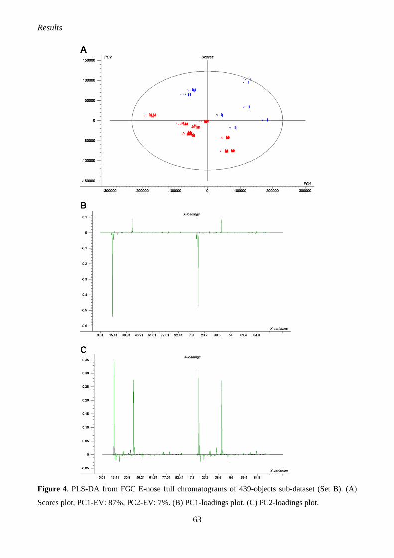
Results
63
Figure 4. PLS-DA from FGC E-nose full chromatograms of 439-objects sub-dataset (Set B). (A)
Scores plot, PC1-EV: 87%, PC2-EV: 7%. (B) PC1-loadings plot. (C) PC2-loadings plot.
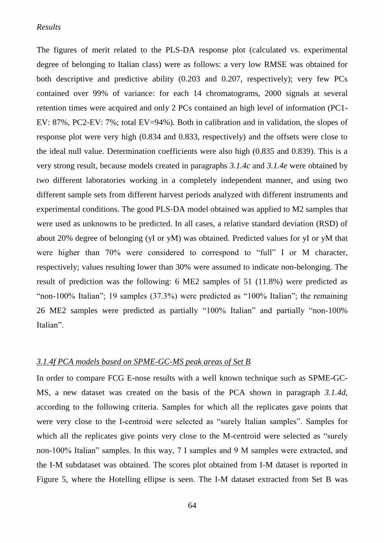
Results
64
The figures of merit related to the PLS-DA response plot (calculated vs. experimental
degree of belonging to Italian class) were as follows: a very low RMSE was obtained for
both descriptive and predictive ability (0.203 and 0.207, respectively); very few PCs
contained over 99% of variance: for each 14 chromatograms, 2000 signals at several
retention times were acquired and only 2 PCs contained an high level of information (PC1-
EV: 87%, PC2-EV: 7%; total EV=94%). Both in calibration and in validation, the slopes of
response plot were very high (0.834 and 0.833, respectively) and the offsets were close to
the ideal null value. Determination coefficients were also high (0.835 and 0.839). This is a
very strong result, because models created in paragraphs 3.1.4c and 3.1.4e were obtained by
two different laboratories working in a completely independent manner, and using two
different sample sets from different harvest periods analyzed with different instruments and
experimental conditions. The good PLS-DA model obtained was applied to M2 samples that
were used as unknowns to be predicted. In all cases, a relative standard deviation (RSD) of
about 20% degree of belonging (yI or yM) was obtained. Predicted values for yI or yM that
were higher than 70% were considered to correspond to “full” I or M character,
respectively; values resulting lower than 30% were assumed to indicate non-belonging. The
result of prediction was the following: 6 ME2 samples of 51 (11.8%) were predicted as
“non-100% Italian”; 19 samples (37.3%) were predicted as “100% Italian”; the remaining
26 ME2 samples were predicted as partially “100% Italian” and partially “non-100%
Italian”.
3.1.4f PCA models based on SPME-GC-MS peak areas of Set B
In order to compare FCG E-nose results with a well known technique such as SPME-GC-
MS, a new dataset was created on the basis of the PCA shown in paragraph 3.1.4d,
according to the following criteria. Samples for which all the replicates gave points that
were very close to the I-centroid were selected as “surely Italian samples”. Samples for
which all the replicates give points very close to the M-centroid were selected as “surely
non-100% Italian” samples. In this way, 7 I samples and 9 M samples were extracted, and
the I-M subdataset was obtained. The scores plot obtained from I-M dataset is reported in
Figure 5, where the Hotelling ellipse is seen. The I-M dataset extracted from Set B was
Results
65
processed by SPME-GC-MS, and careful and detailed analysis of mass spectra was
performed to identify molecules corresponding to significant chromatographic peaks.
Figure 5. Scores plot of FGC E-nose peak areas of I–M dataset (Set B). PC1-EV: 25%, PC2-EV:
16%.
It must be pointed out that neither the gas chromatographic conditions nor the headspace
conditions, employed for SPME-GC-MS and FGC E-nose respectively, were identical.
Moreover, correlation analysis between SPME-GC-MS and FGC E-nose chromatograms
may show eventual correspondences between species identified in SPME-GC-MS and FGC
E-nose retention times. This could help in bypassing the non-target character of FGC E-nose
analyses. Since SPME-GC-MS analyses were performed in two replicates (Set B), the 7+9
samples corresponded to 14+18 objects. The species identified by SPME-GC-MS analysis
were the following: 1-hexanol; 1-octanol; 1-octen-3-ol; 1-penten-3-ol; 1-penten-3-one; 2,4-
decadienal; 2,4-hexadienal; 2-butenal; 2-heptanone; 2-methylbutanal; 2-methylbutanol; 2-
octanol; 3,4-diethyl 1,5-hexadiene; 3,4-diethyl meso-1,5-hexadiene; 3,5-octadien-2-one;
3,7-decadiene; 3-ethyl 1,5-octadiene; 3-methylbutanal; 3-methylbutanol; 3-pentanone;
acetic acid; acetone; γ -copaene; γ -murolene; γ -pinene; benzeneethanol (2-Phenylethanol);
Results
66
benzenemethanol; citronellal; decanal; decane; dimethylnonadienal; (E,E)-γ-farnesene; (E)-
2-heptenal; (E)-2-hexenal; (E)-2-hexenol; (E)-2-pentenal; (E)-2-pentenol; (E)-b-ocimene;
ethanol; ethylacetate; formic acid; hheptanal; hexanal; hexane; hexylacetate; isoamylacetate;
isoamylalcohol; limonene; methanol; methylacetate; methyloctane; murolene; nonanal;
octanal; octane; pentanal; propanal; (Z)-2-pentenol; (Z)-3-hexenal; (Z)-3-hexenol; (Z)-3-
hexenylacetate; (Z)-4,8-dimethylnonatriene. Each of these species was a “variable” in a
dataset created by putting the I-M samples on lines and the SPME-GC-MS peak-area values
(in total ion current, TIC) in the corresponding columns. There were 62 species detected,
although some were detected by both the morepolar and by less-polar columns. Hence, there
were 89 variables in the SPME-GC-MS dataset, which was more than the number of species
detected. The PCA model obtained by the I-M SPME-GC-MS dataset is reported in Figure
6A, where the Hotelling ellipse is seen. An excellent separation was observed between I and
M clusters, thus confirming that headspace GC may discriminate the Italian quality of
EVOOs. The corresponding correlation loadings plot (Figure 6B) showed which species are
especially important in discriminating samples: the molecules in the zone between the
internal and the external ellipses are the most important variables; molecules with absolute
values of loadings higher than 0.3 may be considered significantly relevant. It is interesting
to observe that molecules relevant to a separation along PC1, namely 16 with respect to the
separation between I and M, are due to primary or secondary metabolic compounds of the
LOX pathway and terpenes. This has a chemical-biological basis, since molecules derived
from these enzymatic activities are known to be influenced by the cultivar and geographic
origin. Comparison between Figures 5 and 6A shows that the FGC E-nose peak areas and
SPME-GC-MS peak areas yield a very similar PCA model: this confirms that headspace GC
data (independently of how volatiles are brought into the GC column, i.e. FGC E-nose or
SPME-GC-MS) are suitable for discriminating between 100% Italian and non-100% Italian
samples, and that FGC E-nose performance in this discrimination is not significantly
different with respect to SPME-GC-MS. It must be pointed out that the extraction of the
training set samples from the initial samples was performed based on data pre-processing on
objects obtained by FGC E-nose; the fact that these objects gave good results even with
SPME-GC-MS data demonstrates that the initial choice was not a tautology: MS data are
completely independent from FID data. The comparison between the scores plot and the
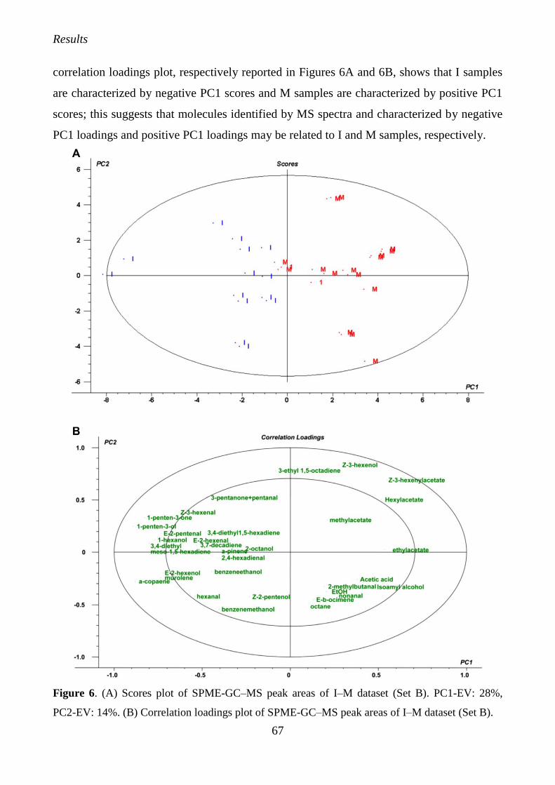
Results
67
correlation loadings plot, respectively reported in Figures 6A and 6B, shows that I samples
are characterized by negative PC1 scores and M samples are characterized by positive PC1
scores; this suggests that molecules identified by MS spectra and characterized by negative
PC1 loadings and positive PC1 loadings may be related to I and M samples, respectively.
Figure 6. (A) Scores plot of SPME-GC–MS peak areas of I–M dataset (Set B). PC1-EV: 28%,
PC2-EV: 14%. (B) Correlation loadings plot of SPME-GC–MS peak areas of I–M dataset (Set B).
Results
68
3.1.4g Correlation between FGC E-nose and SPME-GC-MS data of Set B
In order to study the correlation between FID variables and MS variables, a dataset in which
lines corresponded to the I-M samples discussed in paragraphs 3.1.4d and 3.6f was created;
all columns relevant to FGC E-nose peak areas and SPME-GC-MS peak areas relevant to
the more polar column are reported. The correlation matrix for the FID-peaks and MS-peaks
was calculated, and correlation coefficients with significant or considerable values for
highly discriminating FGC E-nose peaks (see paragraph 3.1.4d) were observed. For
instance, correlation coefficients higher than 0.8 were observed for ethanol, methylacetate,
ethylacetate, 1-penten-3-one, 1-penten-3-ol, (E)-1-hexenal, 1-hexanol, and (E)-2-hexenol.
This analysis shows that accurate study may lead to identification of FGC E-nose peaks,
thus bypassing the shortcomings of this technique: it is a non-target analysis; when a
significant signal is not linkable to a chemical characteristic, the chemometric 17 results are
less strong. It must be underlined that high correlation between retention time and a
molecule does not imply that the molecule is an important variable; the present correlation
analysis simply has an identification purpose. Importance of variables is determined by
loadings: the important molecules are those lying in the outside elliptical ring shown in
correlation loadings plot (Fig. 6B). Complete identification of FGC E-nose signal is beyond
the scope of the present work, which aims to demonstrate that FGC E-nose based
chemometric models are not less reliable that those obtained with SPME-GC-MS data.
3.1.5 Conclusions
This study demonstrates that FGC E-nose is suitable for checking geographical traceability
of EVOO, even using non-target chromatographic signals of the volatile fraction as
variables for multivariate analysis. As a consequence, the feasibility of comparing the
geographic origin of standard EVOOs to the origin of an unknown EVOO using FGC E-
nose chromatograms as a fingerprint has been assessed. A PLS-DA model, able to
discriminate between oils labeled as “100% Italian” (I) and oils labeled as EU oils mixture,
considered as “non-100% Italian" (M), was created. This means that when a good, reliable
training set coming from a certain production year is available, it is possible to verify,
through direct and rapid analysis, whether unknown samples belong to the same statistical
population as the training set. Moreover, it is possible to quantify the degree of belonging of
Results
69
unknown samples to the category “100% Italian”. The performance of geographic
discrimination of FGC E-nose was comparable with SPME-GC-MS, and the results
obtained by the two techniques on the same dataset were not significantly different.
Comparison between FGC E-nose and SPME-GC-MS signals allowed for eventual
correlations between some FGC E-nose retention times and particular molecules identified
by their MS spectra in SPME-GC-MS analysis. Both approaches utilized to analyze volatile
compounds were able to discriminate samples with different geographical origin (M vs. I),
but each offers specific advantages and limitations: SPME-GC-MS provided more reliable
diagnostic information on the identity of compounds thanks to the study of the specific ion
fragment profile and the possibility to consult the library of mass spectra, but a lengthy time
for analysis and for data processing is required. FGC E-nose was a very fast analytical tool
(only 100 seconds of acquisition time and 18 virtually no need for solvents), discriminating
samples with a higher explained variance and allowed for comprehensive data processing
with automatic identification of molecules. These results highlight the potential of FGC E-
nose for rapid control of the compliance of information on geographic origin declared in the
label. This analytical approach seems particularly interesting for food providers, commercial
suppliers, and retailers that intend to avoid media scandals of this sector thanks to a more
efficient protection and promotion of the integrity of the olive oil image. The main effort
concerns the possibility to build, season by season (even by each distributor) an internal or
shared and representative data base to be used to screen and control, year after year, EVOOs
labeled with a specific origin.
3.1.6 Acknowledgements
The authors wish to thank Fernando Gottardi and Martino Barbanera of COOP Italia for
providing the samples, guiding students in carrying out part of the experimental work, and
in sharing their expert knowledge about quality control of olive oil.
Results
70
3.1.7 References
Angerosa F. 2002. Influence of volatile compounds on virgin olive oil quality evaluated by
analytical approaches and sensor panels, European Journal of Lipid Science and
Technology, 104, 639-660.
Aparicio R., Morales M.T. Alonso M.V. 1996. Relationship between volatile compounds and
sensory attributes of olive oils by the sensory wheel. Journal of the American Oil Chemists’
Society, 73, 1253-1264.
Azizian H., Mossoba M.M., Fardin A.R., Delmonte P., Karunathilaka S.R., Kramer J.K.G.
2015. Novel, Rapid Identification, and Quantification of Adulterants in Extra Virgin Olive
Oil Using Near-Infrared Spectroscopy and Chemometrics. Lipids, 50, 705-718.
Ben Temime S., Campeol E., Cioni P.L., Daoud D., Zarrouk M. 2006. Volatile compounds
from Che´toui olive oil and variations induced by growing area, Food Chemistry, 99, 315-
325.
Brereton R.G. 2007. Applied Chemometrics for Scientists. John Wiley & Sons, Chichester,
England.
Cecchi T., Alfei B. 2013. Volatile profiles of Italian monovarietal extra virgin olive oils via
HS-SPME-GC-MS: Newly identified compounds, flavors molecular markers, and terpenic
profile. Food Chemistry, 141, 2025-2035.
Cerretani L., Salvador M.D., Bendini A., Fregapane G. 2008. Relationship between sensory
evaluation performed by Italian and Spanish official panels and volatile and phenolic
profiles of virgin olive oils. Chemosensory Perception, 1, 258-267.
Cimato A., Dello Monaco D., Distante C., Epifani M., Siciliano P., Taurino A.M., Zuppa M.,
Sani G. 2006. Analysis of single-cultivar extra virgin olive oils by means of an Electronic
Nose and HSSPME/ GC-MS methods. Sensors and Actuators, B: Chemical, 114, 674-680.
Commission Implementing Regulation (EU) No 1335/2013 of 13 December 2013, amending
Implementing Regulation (EU) No 29/2012 on marketing standards for olive oil, Official
Journal of the European Union, L 335/14.
Diraman H., Dibeklio-lu H. 2009. Characterization of Turkish virgin olive oils produced from
early harvest olives. JAOCS, Journal of the American Oil Chemists' Society, 86, 663-674.
Results
71
European Community 2008. Commission Regulation No. 640/2008. Amending Regulation
No 2568/91/EEC. Official Journal of the European Community L178,11-16.
European Commission Implementing Regulation 2012. EU No 29/2012 13 January 2012.
Marketing standards for olive oil.
Food and Agriculture Organization of The United Nations World Health Organization. 2003.
Traceability implementation in developing countries, its possibilities and its constraints. A
few case studies. 1-159.
Gallina Toschi T., Bendini A., Lozano-Sanchez J., Segura-Carretero A., Conte L. 2013.
Misdescription of edible oils: Flowcharts of analytical choices in a forensic view, European
Journal of Lipid Science and Technology, 115, 1205-1223.
García-González D.L., Luna G., Morales M.T., Aparicio R. 2009. Stepwise geographical
traceability of virgin olive oils by chemical profiles using artificial neural network models,
European Journal of Lipid Science and Technology, 111, 1003-1013.
Gouvinhas I., De Almeida J.M.M.M., Carvalho T., Machado N., Barros A.I.R.N.A. 2015.
Discrimination and characterisation of extra virgin olive oils from three cultivars in different
maturation stages using Fourier transform infrared spectroscopy in tandem with
chemometrics. Food Chemistry, 174, 226-232.
International Olive Oil Council, Selection of the characteristic descriptors of the designation
of origin. 2005. IOOC/T.20/Doc. no 22.
Kalua C.M., Allen M.S., Bedgood Jr D.R., Bishop A.G., Prenzler P.D., Robards K. 2007.
Olive oil volatile compounds, flavour development and quality: A critical review. Food
Chemistry, 100, 273-286.
Jabeur H., Zribi A., Makni J., Rebai A., Abdelhedi R., Bouaziz M. 2014. Detection of
chemlali extra-virgin olive oil adulteration mixed with soybean oil, corn oil, and sunflower
oil by using GC and HPLC. Journal of Agricultural and Food Chemistry, 62, 4893-4904.
Lerma-García M.J., Cerretani L., Cevoli C., Simó-Alfonso E.F., Bendini A., Gallina Toschi
T. 2010. Use of electronic nose to determine defect percentage in oils. Comparison with
sensory panel results. Sensor and Actuators B - Chemical, 147, 283-289.
Melucci D., Fedi S., Locatelli M., Locatelli C., Montalbani S., Cappelletti M. 2013.
Application of pyrolysisgas chromatography-mass spectrometry and multivariate analysis to
Results
72
study bacteria and fungi in biofilms used for bioremediation. Current Drug Targets, 14,
1023-1033.
Mendes T.O., da Rocha R.A., Porto B.L.S., De Oliveira M.A.L., Dos Anjo, V.D.C., Bell
M.J.V. 2015. Quantification of extra-virgin Olive Oil Adulteration with Soybean Oil: a
comparative Study of NIR, MIR, and Raman Spectroscopy Associated with Chemometric
Approaches. Food Analytical Methods, 8, 2339–2346.
Mildner-Szkudlarz S., Jelen H.H. 2008. The potential of different techniques for volatile
compounds analysis coupled with PCA for the detection of the adulteration of olive oil with
hazelnut oil. Food Chemistry, 110, 751-761.
Morales M.T., Luna G., Aparicio R. 2005. Comparative study of virgin olive oil sensory
defects. Food Chemistry, 91, 293-301.
Ollivier D., Artaud J., Pinatel C., Durbec JP., Guerere M. 2006. Differentiation of French
virgin olive oil RDOs by sensory characteristics, fatty acid and triacylglycerol compositions
and chemometrics. Food Chemistry, 97, 382–393.
Peng Q., Tian R., Chen F., Li B., Gao H. 2015. Discrimination of producing area of Chinese
Tongshan kaoliang spirit using electronic nose sensing characteristics combined with the
chemometrics methods. Food chemistry, 178, 301-305.
Pouliarekou E., Badeka A., Tasioula-Margari M., Kontakos S., Longobardi F., Kontominas
M.G. 2011. Characterization and classification of Western Greek olive oils according to
cultivar and geographical origin based on volatile compounds. Journal of Chromatography
A, 1218, 7534-7542.
Procida G., Giomo A., Cichelli A., Conte L.S. 2005. Study of volatile compounds of
defective virgin olive oils and sensory evaluation: A chemometric approach. Journal of the
Science of Food and Agriculture, 85, 2175-2183.
Sinelli N., Casale M., Di Egidio V., Oliveri P., Bassi D., Tura D., Casiraghi E. 2010. Varietal
discrimination of extra virgin olive oils by near and mid infrared spectroscopy. Food
Research International, 43, 2126-2131.
Taamalli A., Arráez Román D., Zarrouk M., Segura-Carretero A., Fernández-Gutiérrez A.
2012. Classification of 'Chemlali' accessions according to the geographical area using
chemometric methods of phenolic profiles analysed by HPLC-ESI-TOF-MS. Food
Chemistry, 132, 561-566.

Results
73
Vichi S., Pizzale L., Conte L.S., Buxaderas S., Lopez-Tamame E. 2003. Solid phase
microextraction in the analysis of virgin olive oil volatile fraction: characterization of virgin
olive oils from two distinct geographical areas of northern Italy, Journal of agricultural and
Food Chemistry, 51, 6572-6577.
Zunin P., Boggia R., Salvadeo P., Evangelisti F. 2005. Geographical traceability of West
Liguria extra virgin olive oils by the analysis of volatile terpenoid hydrocarbons, Journal of
Chromatography A.,1089, 243-249.
Results
74
3.2 Chemical and sensory characterization of olive oil enriched in lycopene from
tomato by-product: sensory evaluation, chromatographic profile of volatile
compounds and other chemicals
Publication details:
Title: Olive oil enriched in lycopene from tomato by-product through a co-milling process
Authors: Bendini Aa, Di Lecce Ga, Valli Ea, Barbieri Sa, Tesini Fa, and Gallina Toschi Ta,b
a Department of Agricultural and Food Sciences, Alma Mater Studiorum, University of Bologna,
U.O.S. Cesena (FC), Italy b Food Waste Innovation Center, Alma Mater Studiorum, University of Bologna, Bologna, Italy
Published on: International Journal of Food Science and Nutrition. 2015. 66(4), 371–377
3.2.1 Abstract
The aim of this investigation was to produce an olive oil (OO) naturally enriched with
antioxidants, recovering carotenoids, in particular lycopene, using an industrial by-product
of tomato seeds and skin. For this purpose, a technological process in a low-scale industrial
plant to co-mill olives and tomato by-product in de-frosted or freeze-dried forms was
applied and studied with respect to control samples. Preliminary results obtained from two
different experiments were carried out by 40 kg of cultivar Correggiolo olives and 60 kg of
olive blends from different cultivars. In both the experiments, the co-milling showed
significant enrichment in carotenoids, especially in lycopene (mean values of 5.4 and 7.2
mg/kg oil from defrosted and freeze-dried by-products, respectively). The experimental
results demonstrated the possibility to obtain a new functional food naturally enriched in
antioxidant compounds, which might be marketed as ‘‘OO dressing enriched in lycopene’’
or ‘‘condiment produced using olives and tomato by-product’’.
Keywords: Antioxidants; co-milling; lycopene; olives; tomato by-product.
Results
75
3.2.2 Introduction
Carotenoids are important lipid-soluble plant pigments involved in photosynthesis and
photo-protection from excessive light. Among these, lycopene, an acyclic carotenoid which
contains conjugated double bonds arranged linearly in situ typically in the all-trans form,
has numerous biological properties, mainly linked to its antioxidant (single oxygen
quenching and radical scavenging) and anti-inflammatory properties (Kaulmann et al.,
2013), that are beneficial for human health. Lycopene is found in plasma and tissues of the
human body, including skin, where it seems to exert an effective action in detoxifying free
radicals and protecting from damage caused by UV and photo-aging (Cazzola, 2012).
Several epidemiological studies have suggested that an adequate intake of lycopene may
reduce the risk of cancer and chronic diseases (Rao et al., 1999; Stahl et al., 1996), even if
the EFSA Panel in 2011 concluded that a clear cause and effect relationship has not been
established yet (EFSA, 2011). Specific research has shown that an increase in dietary
lycopene produces an increase in serum lycopene irrespective of the amount of fat intake.
Moreover, a diet high in olive oil (OO) and rich in lycopene may decrease the risk of
coronary heart disease by improving the serum lipid profile (Ahuja et al., 2006). The role of
antioxidants in human nutrition and their associated health-beneficial effects for a number
of chronic diseases, including certain types of cancer and cardiovascular diseases, have
gained increased attention. There is a particular interest in components of the so-called
‘‘Mediterranean diet’’, such as tomato and OO, which have been associated with a healthier
lifestyle (Capanoglu et al., 2010). Tomatoes and OO are rich sources of key antioxidant
components such as carotenoids, tocopherols and polyphenols, but their amounts may vary
greatly in relation to the adoption of different agronomic, climatic and technological
variables (Frusciante et al., 2007; Morello` et al., 2006; Servili et al., 2004; Dumas et al.,
2003). These fruits are consumed both as fresh products and after processing (mechanical
and thermal treatments for tomato products) or used for cooking. Processing and addition of
ingredients can influence the bioavailability of antioxidants originally present in both
tomatoes and OO (Kamiloglu et al., 2013). In the industrial processing of tomatoes, 10–30%
of their weight is waste constituted by peel and seeds; it is well known that lycopene and
phenolic compounds are more concentrated in the peel than in the pulp (Montesano et al.,
2006; Knoblich et al., 2005; Toor et al., 2005; George et al., 2004). The predominant form
Results
76
of lycopene in tomato products is the all-trans isomer, but, after consumption, lycopene is
biologically converted to various cis isomers; this isomerization process also occurs
naturally during storage and heating treatments. Lycopene is industrially produced by
chemical synthesis or extracted from vegetable sources, mainly tomatoes, using chemical
solvents and referred to as natural lycopene. Clinical studies showed that dietary
supplements made with natural lycopene are more effective than those containing its
synthetic form, probably for the presence of other bio-active molecules co-extracted from
tomatoes, as which synergize with lycopene in promoting the positive effects on human
health (Cazzola, 2012). However, the use of organic solvents for the extraction of natural
lycopene may contaminate the end-product and facilitate the co-extraction of toxic
chemicals including fertilizers, pesticides and heavy metals (Rescio et al., 2010). Several
studies demonstrated the advantages of the lycopene added in a lipid matrix. Montesano and
coworkers (2006) prepared two concentrations (0.5 and 1mg of pure lycopene per 100 g of
oil) of lycopene extracted from tomato in extra virgin olive oil (EVOO) and monitored the
chemical physical changes of samples for 37 weeks; the main results showed a lower rate of
oxidation as well as greater protection of phenolic molecules in oils enriched with pure
lycopene than in the control sample. Benakmoum and co-authors (2008), taking advantage
of their lipophilic properties, incorporated carotenoids in EVOO and refined OO by
preparing mixtures at different proportions (from 5 to 30%) with lyophilized peel thanks to
a 24-h diffusion step. In their oil preparations, the authors detected rutin and naringenin as
flavonoids coming exclusively from tomato peel and verified enrichment in lycopene and b-
carotene. Such positive results have encouraged the marketing of new lycopene containing
products sold as functional food, often prepared by adding lycopene extracted from
tomatoes to lipid matrices from vegetable or animal origin. Based on previous trials
(Cerretani et al., 2008), a low-scale mill to process together olives and tomato by-product
(in defrosted or freeze-dried form) has been used in this investigation. Specifically, in the
present study, the co-milling of olive paste and tomato by-product was finalized to verify
the potential of minor compounds releasing, especially carotenoids, allowing the production
of an oil fraction enriched with such antioxidants.
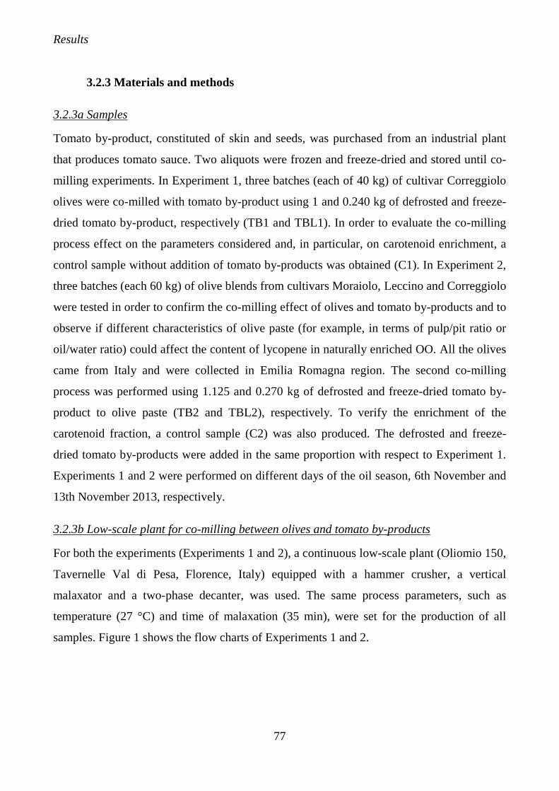
Results
77
3.2.3 Materials and methods
3.2.3a Samples
Tomato by-product, constituted of skin and seeds, was purchased from an industrial plant
that produces tomato sauce. Two aliquots were frozen and freeze-dried and stored until co-
milling experiments. In Experiment 1, three batches (each of 40 kg) of cultivar Correggiolo
olives were co-milled with tomato by-product using 1 and 0.240 kg of defrosted and freeze-
dried tomato by-product, respectively (TB1 and TBL1). In order to evaluate the co-milling
process effect on the parameters considered and, in particular, on carotenoid enrichment, a
control sample without addition of tomato by-products was obtained (C1). In Experiment 2,
three batches (each 60 kg) of olive blends from cultivars Moraiolo, Leccino and Correggiolo
were tested in order to confirm the co-milling effect of olives and tomato by-products and to
observe if different characteristics of olive paste (for example, in terms of pulp/pit ratio or
oil/water ratio) could affect the content of lycopene in naturally enriched OO. All the olives
came from Italy and were collected in Emilia Romagna region. The second co-milling
process was performed using 1.125 and 0.270 kg of defrosted and freeze-dried tomato by-
product to olive paste (TB2 and TBL2), respectively. To verify the enrichment of the
carotenoid fraction, a control sample (C2) was also produced. The defrosted and freeze-
dried tomato by-products were added in the same proportion with respect to Experiment 1.
Experiments 1 and 2 were performed on different days of the oil season, 6th November and
13th November 2013, respectively.
3.2.3b Low-scale plant for co-milling between olives and tomato by-products
For both the experiments (Experiments 1 and 2), a continuous low-scale plant (Oliomio 150,
Tavernelle Val di Pesa, Florence, Italy) equipped with a hammer crusher, a vertical
malaxator and a two-phase decanter, was used. The same process parameters, such as
temperature (27 °C) and time of malaxation (35 min), were set for the production of all
samples. Figure 1 shows the flow charts of Experiments 1 and 2.
Results
78
Figure 1. Flowchart of co-milling processes: Experiments 1 and 2. C: control sample, obtained
crushing only the olives; TB: sample obtained by crushing olives with defrosted tomato by-product;
TBL: sample obtained by crushing olives with freeze-dried tomato by-product, as explained in
‘‘Samples’’ section.
3.2.3c Quality indices determination
Determination of the physicochemical quality parameters (free acidity, peroxide value, UV
specific extinction at 232 and 270 nm) was carried out according to the respective official
methods (EEC 2568/91 and following amendments).
3.2.3d Sensory analysis
The IOC panel test was carried out by eight selected and trained panelists, all members of
the Bologna University professional committee (panel DISTAL), which is recognized by the
Italian Government. Evaluation of samples was performed under the conditions described in
EU Regulation 1348/2013; if secondary positive attributes were perceived, the taster
recorded them using the list of sensory descriptors according to the IOC document
(IOOC/T.20/Doc. no 22, 2005).
Results
79
3.2.3e Extraction of phenolic fraction and spectroscopic determination of ortho-diphenols
Extraction of polar minor compounds followed the protocol described by Pirisi et al. (2000)
and modified according to Rotondi et al. (2004). Two aliquots of oil (2 g) were added to
1ml of n-hexane and 2ml of a methanol/water (60:40, v/v), mixed and centrifuged for 3 min
at 3000 rpm (907.2 x g). The hydroalcoholic extract was collected, and the oil phase was re-
extracted twice with 2ml of methanol/water (60:40, v/v) solution each time. Finally, all the
hydroalcoholic fractions were combined, washed with 2ml of n-hexane to remove the
residual oil, then concentrated and evaporated under vacuum at 35 °C. The dry extracts were
diluted in 0.5 ml of a methanol/water (50:50, v/v) solution and filtered through a 0.2-mm
nylon filter. Extractions were performed in three replicates, and extracts were stored at -18
°C before analysis. The content of total o-diphenols (o-DIPH) was spectrophotometrically
evaluated, according to Mateos et al. (2001) at 370 nm and against a reference prepared with
the same procedure, but without adding the phenolic extract. A specific calibration curve
(r2=0.993) was built to express the data as mg gallic acid kg-1 of oil.
3.2.3f HPLC analysis of individual phenolic components
Analysis of the phenolic profile was performed according to the COI/T.20/Doc No. 29
(2009) protocol, with some modifications related to the chromatographic analysis. The
method provides for direct extraction of the phenolic fraction from OO using a methanol
solution and subsequent quantification by HPLC coupled to an UV detector at 280 nm.
Syringic acid was used as the internal standard, while the content of the individually
identified phenolic compounds was expressed as tyrosol (mg kg-1). The chromatographic
analysis was performed using a 1260 series HPLC instrument equipped with a quaternary
pump (Agilent Technologies, Waldbronn, Germany) and a reverse phase C18 100A Kinetex
column (2.6 mm, 100x3.00mm I.D., Phenomenex, Torrance, CA). The elution gradient was
carried out with a solvent system of water/formic acid (99.5:0.5 v/v) as mobile phase A and
acetonitrile as mobile phase B; the total runtime was 13 min and the gradient elution was as
follows: from 0 to 3 min solvent B increased from 5 to 20%, at 4 min solvent B reached
40%, at 9 min solvent B reached 60%, and finally at 10 min solvent B at 100%; at 13 min,
5% solvent B was restored. The column was thermostated at 30 °C and equilibrated for 5
min prior to each analysis; an injection volume of 5 ml and a flow rate of 0.7 ml min-1 were
Results
80
used. The main phenolic compounds were tentatively identified based on mass spectra using
a mass spectrometer (MS, Agilent, Phoenix, AZ) in electrospray ionization mode. The MS
working conditions were: nebulizer gas pressure, 0.24 MPa; drying gas flow, 7l min-1 at 300
°C; capillary voltage, 2.5 kV; voltages of skimmers 1 and 2, -41.0 and -6.0V, respectively.
Nitrogen was used as a nebulizer and drying gas. The MS was scanned within the m/z 100–
900 range in the negative and positive ion mode.
3.2.3g Carotenoid extraction from tomato by-products
Aliquots of defrosted and freeze-dried tomato waste were subjected to the extraction of
carotenoids to define the quantity of tomato by-products to be added during the co-milling
experiment and to evaluate the migration of carotenoid compounds. The extraction of
carotenoids was carried out in darkness, using an ice bath according to Vallverdù-Queralt et
al. (2012) to minimize the oxidation phenomena. Defrosted and freeze-dried tomato by-
product (2 g) were homogenized for 1 min with 5ml of ethanol/n-hexane (4:3, v/v) using an
Ultra-Turrax at 5000 rpm (2520 x g), sonicated for 5 min and centrifuged at 4000 rpm (1613
x g) for 10 min. The extraction procedure was repeated twice, and the collected supernatants
were combined and evaporated under nitrogen flow. Finally, the residue was reconstituted
with methanol and methyl-tert-butyl ether (2:1), filtered through 0.45 mm PTFE filter and
analyzed by HPLC as described below.
3.2.3h Lutein, β-carotene and lycopene analysis
The carotenoid fraction was extracted and purified from OO samples according to the
saponification procedure described for sterol determination in the official method (EEC
2568/91 and following amendments): the oil was saponified with potassium hydroxide in
ethanolic solution, and the unsaponifiable matter was then extracted with diethyl ether. The
unsaponifiable fraction was recollected in a 5-ml of n-hexane and i-propanol (4:1 v/v) and
stored at -18 °C. Before HPLC analysis, 0.5 ml of n-hexane/i-propanol solution was
evaporated and dissolved in 0.5 ml of methanol and methyl-tertbuthylether (2:1 v/v). The
solution was vortexed and filtered with a 0.45-mm nylon filter. HPLC analysis was
performed using an Agilent 1200 Series HPLC system (Hewlett-Packard, Waldbronn,
Germany) with a C18 Zorbax Eclipse plus column (4.6 x 250 mm, particle size 5 mm,
Agilent, Phoenix, AZ). The elution solvents used were A (methanol/1% ammonium acetate)
Results
81
and B (methyl-tert-buthyl ether), and the targeted compounds were eluted according to the
following gradient: starting from 100% A, increased to 20% B in 20 min, and percentage
was maintained for 5 min. The flow rate was 1 ml min-1 and the sample injection volume
was 20 mL. Detection was at 470 nm. Identification of carotenoids was achieved by
comparing the retention times with pure standards of LUT, b-CAR and lycopene (Fluka,
Sigma-Aldrich, Steinheim, Germany), and their concentrations in samples were calculated
using the respective calibration curves prepared using different concentrations of standard
solutions (r2=0.999, r2=0.995 and r2=0.998, respectively).
3.2.3i Tocopherol determination
Briefly, 0.5 g of oil sample were added into a 10-ml volumetric flask and brought to volume
with i-propanol. The solution was filtered through a 0.45-mm nylon filter paper before
HPLC-DAD analysis, which was performed with the same apparatus described previously.
Detection was performed at 292 nm. The column was a Cosmosil π NAP 150mm x 4.6 mm,
5 mm particle size (Nacalai-Tesque, Kyoto, Japan). The elution solvents used were: A
(methanol/water, 90/10 v/v acidified with 0.2% H3PO4) and B (acetonitrile). The samples
were eluted according to the following gradient: 100% A for 22 min; 100% B for 13 min;
100% A maintained for 15 min. The flow rate was 1 ml min-1. The sample injection volume
was 10 ml. Identification of a-TOC (Fluka, Sigma-Aldrich, Steinheim, Germany) was
developed by comparing the retention time of a pure standard, and its concentration in
samples was calculated using the calibration curve constructed using solutions of a-TOC at
different concentrations (r2=0.999).
3.2.3l Volatile compounds analysis
Analysis was performed by SPME-GC-MS according to the procedure described by
Baccouri et al. (2008); SPME fibers were coated with a
divinylbenzene/carboxen/polydimethylsiloxane (DVB/CAR/PDMS) phase (50/30 mm, 2 cm
long from Supelco Ltd., Bellefonte, PA), and 4-methyl-2-pentanone (Fluka, Sigma-Aldrich,
Steinheim, Germany) was added as an internal standard. Volatile compounds were
identified and quantified by GC (Agilent 6890N) coupled with a quadrupolar MS (Agilent
5973N, Agilent Technologies, Phoenix, AZ). Analytes were separated on a column of 30 m,
0.25mm i.d., 1.00 mm f.t. (Phenomenex) coated with polyethylene glycol phase. The
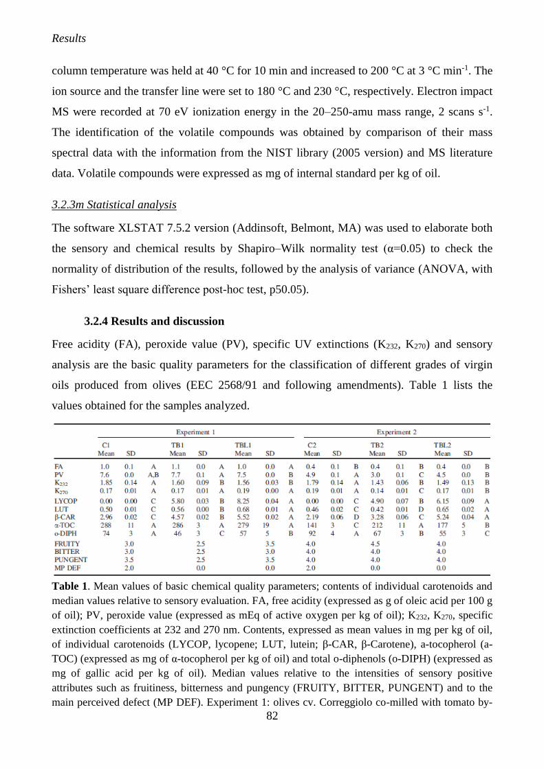
Results
82
column temperature was held at 40 °C for 10 min and increased to 200 °C at 3 °C min-1. The
ion source and the transfer line were set to 180 °C and 230 °C, respectively. Electron impact
MS were recorded at 70 eV ionization energy in the 20–250-amu mass range, 2 scans s-1.
The identification of the volatile compounds was obtained by comparison of their mass
spectral data with the information from the NIST library (2005 version) and MS literature
data. Volatile compounds were expressed as mg of internal standard per kg of oil.
3.2.3m Statistical analysis
The software XLSTAT 7.5.2 version (Addinsoft, Belmont, MA) was used to elaborate both
the sensory and chemical results by Shapiro–Wilk normality test (α=0.05) to check the
normality of distribution of the results, followed by the analysis of variance (ANOVA, with
Fishers’ least square difference post-hoc test, p50.05).
3.2.4 Results and discussion
Free acidity (FA), peroxide value (PV), specific UV extinctions (K232, K270) and sensory
analysis are the basic quality parameters for the classification of different grades of virgin
oils produced from olives (EEC 2568/91 and following amendments). Table 1 lists the
values obtained for the samples analyzed.
Table 1. Mean values of basic chemical quality parameters; contents of individual carotenoids and
median values relative to sensory evaluation. FA, free acidity (expressed as g of oleic acid per 100 g
of oil); PV, peroxide value (expressed as mEq of active oxygen per kg of oil); K232, K270, specific
extinction coefficients at 232 and 270 nm. Contents, expressed as mean values in mg per kg of oil,
of individual carotenoids (LYCOP, lycopene; LUT, lutein; β-CAR, β-Carotene), a-tocopherol (a-
TOC) (expressed as mg of α-tocopherol per kg of oil) and total o-diphenols (o-DIPH) (expressed as
mg of gallic acid per kg of oil). Median values relative to the intensities of sensory positive
attributes such as fruitiness, bitterness and pungency (FRUITY, BITTER, PUNGENT) and to the
main perceived defect (MP DEF). Experiment 1: olives cv. Correggiolo co-milled with tomato by-
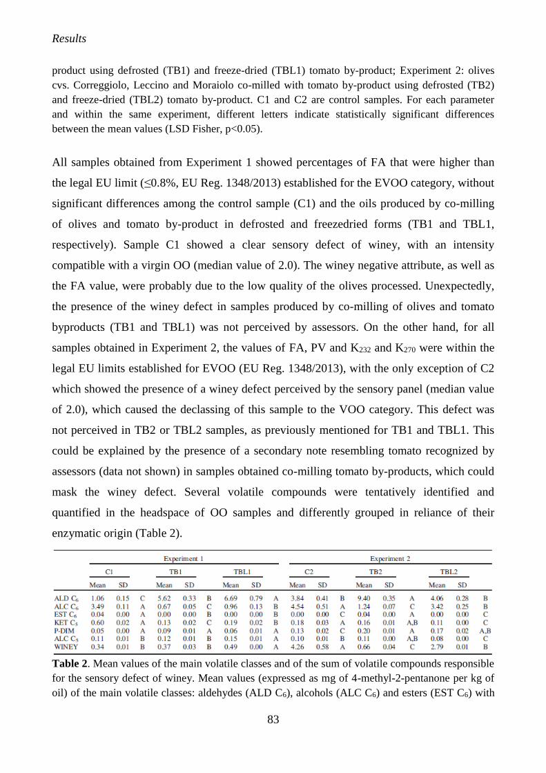
Results
83
product using defrosted (TB1) and freeze-dried (TBL1) tomato by-product; Experiment 2: olives
cvs. Correggiolo, Leccino and Moraiolo co-milled with tomato by-product using defrosted (TB2)
and freeze-dried (TBL2) tomato by-product. C1 and C2 are control samples. For each parameter
and within the same experiment, different letters indicate statistically significant differences
between the mean values (LSD Fisher, p<0.05).
All samples obtained from Experiment 1 showed percentages of FA that were higher than
the legal EU limit (≤0.8%, EU Reg. 1348/2013) established for the EVOO category, without
significant differences among the control sample (C1) and the oils produced by co-milling
of olives and tomato by-product in defrosted and freezedried forms (TB1 and TBL1,
respectively). Sample C1 showed a clear sensory defect of winey, with an intensity
compatible with a virgin OO (median value of 2.0). The winey negative attribute, as well as
the FA value, were probably due to the low quality of the olives processed. Unexpectedly,
the presence of the winey defect in samples produced by co-milling of olives and tomato
byproducts (TB1 and TBL1) was not perceived by assessors. On the other hand, for all
samples obtained in Experiment 2, the values of FA, PV and K232 and K270 were within the
legal EU limits established for EVOO (EU Reg. 1348/2013), with the only exception of C2
which showed the presence of a winey defect perceived by the sensory panel (median value
of 2.0), which caused the declassing of this sample to the VOO category. This defect was
not perceived in TB2 or TBL2 samples, as previously mentioned for TB1 and TBL1. This
could be explained by the presence of a secondary note resembling tomato recognized by
assessors (data not shown) in samples obtained co-milling tomato by-products, which could
mask the winey defect. Several volatile compounds were tentatively identified and
quantified in the headspace of OO samples and differently grouped in reliance of their
enzymatic origin (Table 2).
Table 2. Mean values of the main volatile classes and of the sum of volatile compounds responsible
for the sensory defect of winey. Mean values (expressed as mg of 4-methyl-2-pentanone per kg of
oil) of the main volatile classes: aldehydes (ALD C6), alcohols (ALC C6) and esters (EST C6) with
Results
84
six carbon atoms originating from the LOX pathway; ketones (KET C5), alcohols (ALC C5) with
five carbon atoms and pentene dimers (P-DIM) originating from the secondary pathway of LOX.
Mean values of the sum of volatile compounds considered to be responsible for the main perceived
sensory defect of WINEY (methyl acetate, ethyl acetate, methanol, ethanol and acetic acid).
Experiment 1: olives cv. Correggiolo co-milled with tomato by-product using defrosted (TB1) and
freeze-dried (TBL1) tomato by-product; Experiment 2: olives cvs. Correggiolo, Leccino and
Moraiolo co-milled with tomato by-product using defrosted (TB2) and freeze-dried (TBL2) tomato
by-product. C1 and C2 are control samples. For each parameter and within the same experiment,
different letters indicate statistically significant differences between the mean values (LSD Fisher,
p<0.05).
According to other authors (Angerosa et al., 2004, 2000), C6 and C5 volatile molecules
coming from the lipoxygenase enzymatic pathway have been primarily considered to be
those mainly responsible for the odor notes of EVOO. The group of C6 compounds derived
by the primary LOX pathway have been distinguished in aldehydes (ALD C6), alcohols
(ALC C6), esters (EST C6) and the group of C5 compounds derived by the secondary LOX
pathway in ketones (KET C5), alcohols (ALC C5) and pentene dimers (P-DIM). Generally,
for all samples, the C6 compounds, and, in particular, ALD C6, were the most abundant, but,
in the case of the two samples judged as defective by sensory analysis (C1 and C2), a higher
content in ALC C6 was found. In a previous study (Bendini et al., 2007), a lower ratio of
ALD C6 to ALC C6 was detected in samples characterized by lower intensity of green notes
and the presence of unpleasant olfactory perceptions. In particular, C2 was also
characterized by the highest concentration of compounds that have been related to the
sensory defect of winey, such as those linked to sugar fermentation (ethanol, ethylacetate
and acetic acid) and overripe olives (methanol and methylacetate). There was no clear
evidence of a predominance of specific molecules or of a class of compounds in the volatile
profiles of samples produced by co-milling of olives and tomato by-product. Table 3
includes the polar phenolic compounds identified and quantified in all samples by HPLC-
DAD-MS. A total of eight compounds belonging to phenolic acids, phenolic alcohols and
secoiridoids were tentatively identified. For Experiment 1, the co-milling process did not
affect the total phenolic content (TOT PH), but the behavior of selected individual polar
phenols showed significant differences depending on the type of sample. The highest
concentrations of the oxidized form of decarboxymethyl oleuropein aglycone (ox-DOA)
were detected in both the co-milled samples, whereas the content of ligstroside aglycone
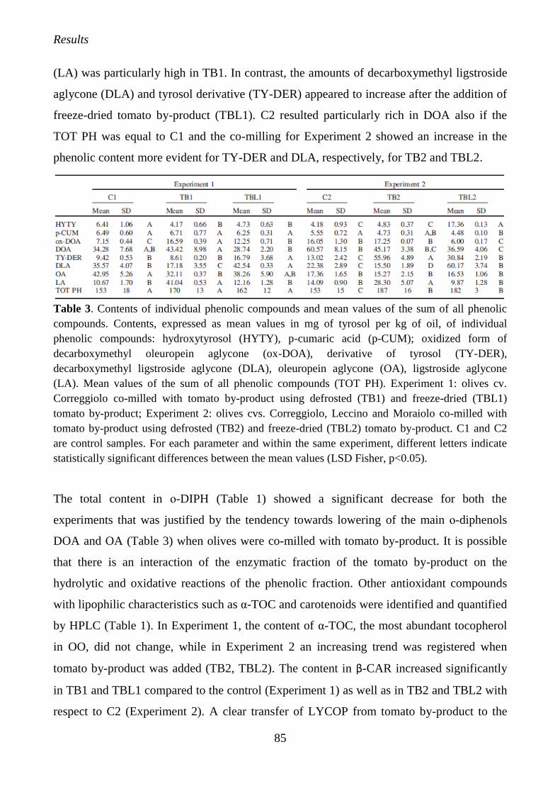
Results
85
(LA) was particularly high in TB1. In contrast, the amounts of decarboxymethyl ligstroside
aglycone (DLA) and tyrosol derivative (TY-DER) appeared to increase after the addition of
freeze-dried tomato by-product (TBL1). C2 resulted particularly rich in DOA also if the
TOT PH was equal to C1 and the co-milling for Experiment 2 showed an increase in the
phenolic content more evident for TY-DER and DLA, respectively, for TB2 and TBL2.
Table 3. Contents of individual phenolic compounds and mean values of the sum of all phenolic
compounds. Contents, expressed as mean values in mg of tyrosol per kg of oil, of individual
phenolic compounds: hydroxytyrosol (HYTY), p-cumaric acid (p-CUM); oxidized form of
decarboxymethyl oleuropein aglycone (ox-DOA), derivative of tyrosol (TY-DER),
decarboxymethyl ligstroside aglycone (DLA), oleuropein aglycone (OA), ligstroside aglycone
(LA). Mean values of the sum of all phenolic compounds (TOT PH). Experiment 1: olives cv.
Correggiolo co-milled with tomato by-product using defrosted (TB1) and freeze-dried (TBL1)
tomato by-product; Experiment 2: olives cvs. Correggiolo, Leccino and Moraiolo co-milled with
tomato by-product using defrosted (TB2) and freeze-dried (TBL2) tomato by-product. C1 and C2
are control samples. For each parameter and within the same experiment, different letters indicate
statistically significant differences between the mean values (LSD Fisher, p<0.05).
The total content in ο-DIPH (Table 1) showed a significant decrease for both the
experiments that was justified by the tendency towards lowering of the main ο-diphenols
DOA and OA (Table 3) when olives were co-milled with tomato by-product. It is possible
that there is an interaction of the enzymatic fraction of the tomato by-product on the
hydrolytic and oxidative reactions of the phenolic fraction. Other antioxidant compounds
with lipophilic characteristics such as α-TOC and carotenoids were identified and quantified
by HPLC (Table 1). In Experiment 1, the content of α-TOC, the most abundant tocopherol
in OO, did not change, while in Experiment 2 an increasing trend was registered when
tomato by-product was added (TB2, TBL2). The content in β-CAR increased significantly
in TB1 and TBL1 compared to the control (Experiment 1) as well as in TB2 and TBL2 with
respect to C2 (Experiment 2). A clear transfer of LYCOP from tomato by-product to the
Results
86
produced oils was also detected. In Experiment 1, a high percentage of lycopene passed
from the by-product to the oils, with recoveries of 80.3% (TB1) and 92.6% (TBL2). Lower
percentages were found in Experiment 2, in which the recoveries were 66.3% and 69.8% for
TB2 and TBL2, respectively. In general, both the experiments performed by co-milling
between olive paste and freeze-dried tomato by-product (TBL1 and TBL2) produced the
highest contents of all carotenoids. In this regard, the use of tomato by-product in freeze-
dried form, in comparison to the one that was simply de-frosted, may represent a better way
to produce a ‘‘naturally enriched OO’’ with a higher concentration of lycopene. On the
other hand, differences in terms of quality parameters, volatiles and phenolic compounds
could be highlighted between samples in Experiments 1 and 2; this might be related to the
quality of the olives themselves and, in particular, to the characteristics that each specific
cultivar gave to the OO.
3.2.5 Conclusions
Different factors, mainly the cost of disposing of waste, the appeal of natural additives for
the food industry and increased legislative restrictions to protect the environment have
contributed over the last few years to the development of improved waste-handling
technology. Concerning agro-industrial tomato by-products, many applications for their re-
use and valorization have already been proposed, for example, in animal feed thanks to the
considerable content of protein and carotenoid (Knoblich et al., 2005; Toor et al., 2005) and
for enrichment of low-quality edible oils (Benakmoum et al., 2008). The present
investigation suggests the possibility to use the industrial tomato by-product (skin and
seeds) for co-milling with olives to obtain a vegetable oil that is naturally rich in
antioxidants, especially in carotenoids. Specifically, the presence of lycopene in this
functional food takes origin from the tomato by-product thanks to transfer of this lipophilic
molecule into the lipid matrix only through a mechanical process, different from maceration
and avoiding the use of solvents or chemicals. This new product might be marketed as a
‘‘condiment produced using olives and tomato by-products’’ or ‘‘OO dressing enriched in
lycopene’’. Further research should be carried out to evaluate if the freeze-dried form of
tomato by-products is more suitable than the defrosted one considering both the efficacy of
antioxidant transfer and economic viewpoints.
Results
87
3.2.6 References
Ahuja K.D.K., Pittaway J.K., Ball M.J. 2006. Effects of olive oil and tomato lycopene
combination on serum lycopene, lipid profile, and lipid oxidation. Nutrition, 22, 259–265.
Angerosa F., Mostallino R., Basti C., Vito R. 2000. Virgin olive oil odour notes: their
relationships with volatile compounds from the lipoxygenase pathway and secoiridoid
compounds. Food Chemistry, 68, 283–287.
Angerosa F., Servili M., Selvaggini R., Taticchi A., Esposto S., Montedoro G.F. 2004.
Volatile compounds in virgin olive oil: occurrence and their relationship with quality.
Journal of Chromatography A, 1054, 17–31.
Baccouri O., Bendini A., Cerretani L., Guerfel M., Baccouri B., Lercker G., Zarrouk M.,
Daoud Ben Miled D. 2008. Comparative study on volatile compounds from Tunisian and
Sicilian monovarietal virgin olive oils. Food Chemistry, 111, 322–328.
Benakmoum A., Abbeddou S., Ammouche A., Kefalas P., Gerasopoulos D. 2008.
Valorisation of low quality edible oil with tomato peel waste. Food Chemistry 110:684–690.
Bendini A., Cerretani L., Lercker G. 2007. Survey on the quality of virgin olive oils produced
in Romagna. Rivista Italiana delle Sostanze Grasse, 84, 191–202.
Capanoglu E., Beekwilder J., Boyacioglu D., De Vos R.C.H., Hall R.D. 2010. The effect of
industrial food processing on potentially health-beneficial tomato antioxidants. Critical
Review Food Science Nutrition 50, 919–930.
Cazzola P. 2012. Lycopene: biological activity and use perspectives in dermatology. Journal
of Plastic Dermatology, 8, 199–210.
Cerretani L., Bendini A., Poerio A., Gallina Toschi T. 2008. Citric acid as co-adjuvant:
improvement of the antioxidant activity of edible olive oils. Agro Food Industry Hi-Tech,
19, 64–66.
COI/T.20/Doc No. 29. November 2009. Methods adopted by the International Olive Council
for chemical analysis of olive oils and olive-pomace oils. Determination of biophenols in
olive oils by HPLC. p. 1–8.
Commission Implementing Regulation (EU) No. 1348/2013. Amending regulation (EEC) no.
2568/91 on the characteristics of olive oil and olive-residue oil and on the relevant methods
of analysis. Off Journal of European Union L 338, 17 December 2013, p. 31–67.
Results
88
Consolidated TEXT produced by the CONSLEG system of the Office for Official
Publications of the European Communities (CONSLEG:1991R2568 – 01/11/2003) relative
to the EEC No 2568/91 of 11 July 1991 on the characteristics of olive oil and olive-residue
oil and on the relevant methods of analysis.
Dumas Y., Dadomo M., Di Lucca G., Grolier P. 2003. Effects of environmental factors and
agricultural techniques on antioxidant content of tomatoes. Journal of Science Food
Agriculture, 83, 369–382.
EFSA. 2011. 9(4), 2031 ‘‘Scientific opinion on the substantiation of health claims related to
lycopene and protection of DNA, proteins and lipids from oxidative damage, protection of
the skin from UV-induced (including photo-oxidative) damage, contribution to normal
cardiac function, and maintenance of normal vision pursuant to Article 13(1) of Regulation
(EC) No 1924/2006’’.
Frusciante L., Carli P., Ercolano M.R., Pernice R., Di Matteo A., Fogliano V., Pellegrini N.
2007. Antioxidant nutritional quality of tomato. Molecular Nutrition Food Research, 51,
609–617.
George B., Kaur C., Khurdiya D.S., Kapoor H.C. 2004. Antioxidants in tomato
(Lycopersicon esculentum) as a function of genotype. Food Chemistry, 84, 45–51.
International Olive Oil Council. 2005. Selection of the characteristic descriptors of the
designation of origin. IOOC/T.20/Doc. no 22.
Kamiloglu S., Boyacioglu D., Capanoglu E. 2013. The effect of food processing on
bioavailability of tomato antioxidants. Journal of Berry Research, 3, 5–77.
Kaulmann A., Bohn T. 2013. Carotenoids, inflammation, and oxidative stress-implications of
cellular signaling pathways and relation to chronic disease prevention. Nutrition Research
34, 907–929.
Knoblich M., Anderson B., Latshaw D. 2005. Analyses of tomato peel and seed by-products
and their use as a source of carotenoids. Journal of Food Science and Agriculture, 85, 1166–
1170.
Mateos R., Espartero JL., Trujillo M., Rı`os JJ., Le´on-Camacho M., Alcudia F., Cert A.
2001. Determination of phenols, flavones, and lignans in virgin olive oils by solid-phase
extraction and highperformance liquid chromatography with diode array ultraviolet
detection. Journal of Agricultural and Food Chemistry, 49, 2185–2192.
Results
89
Montesano D., Cossignani L., D’Arco G., Simonetti MS., Damiani P. 2006. Pure lycopene
from tomato preserves extra virgin olive oil from natural oxidative events during storage.
Journal of American Oil Chemists Society, 83, 933–941.
Morello` JR., Romero MP., Motilva MJ. 2006. Influence of seasonal conditions on the
composition and quality parameters of monovarietal virgin olive oils. Journal of American
Oil Chemists Society, 83, 683–688.
Pirisi FM., Cabras P., Falqui Cao C., Migliorini M., Mugelli M. 2000. Phenolic compounds
in virgin olive oil. 2. Reappraisal of the extraction, HPLC separation, and quantification
procedures. Journal of Agricultural and Food Chemistry, 48, 1191–1196.
Rao AV., Agarwal S. 1999. Role of lycopene as antioxidant carotenoid in the prevention of
chronic diseases: a review. Nutrition Research, 19, 305–323.
Rescio L., Di Maio A., Cazzola P. 2010. Lycopene, photo protection and skin care: the
benefits of organic quality. Journal of Plastic Dermatology, 6, 37–47.
Rotondi A., Bendini A., Cerretani L., Mari M., Lercker G., Gallina Toschi T. 2004. Effect of
olive ripening degree on the oxidative stability and organoleptic properties of cv. Nostrana
di Brisighella extra virgin olive oil. Journal of Agricultural and Food Chemistry, 52, 3649–
3654.
Servili M., Selvaggini R., Esposto S., Taticchi A., Montedoro GF., Morozzi G. 2004. Health
and sensory properties of virgin olive oil hydrophilic phenols: agronomic and technological
aspects of production that affect their occurrence in the oil. Journal of Chromatography A,
1054, 113–127.
Stahl W., Sies H. 1996. Lycopene: a biologically important carotenoid for humans? Archive
of Biochemistry and Biophyicss, 336, 1–9.
Toor RK., Savage GP. 2005. Antioxidant activity in different fractions of tomatoes. Food
Research International, 38, 487–494.
Vallverdu´-Queralt A., Arranz S., Casals-Ribes I., Lamuela-Ravento´s R.M. 2012. Stability
of the phenolic and carotenoid profile of gazpachos during storage. Journal of Agricultural
and Food Chemistry, 60, 1981-1988.
Results
90
3.3 Identification and quanification of volatile compounds in differently processed
faba beans and relation with sensory aspects
3.3.1 Abstract
Faba bean is one of the world’s oldest cultivated plants. Its nutritional and sensory profiles
have been studied, but off-flavours, related to the processing of beans, frequently occur.
They have to be taken into account in in order to optimise sensory characteristics and
nutritional value. In the present study, the aroma profiles of native, conventionally oven
heated and microwave treated faba bean samples were studied as flour, suspensions, extracts
and emulsions with different amounts of oil. The aroma profiles were investigated by
volatile compounds identification and quantification and by sensory analysis. The results of
this work highlighted how samples produced with thermally treated beans showed the
presence of volatile compounds produced during autoxidation processes and perceived by
panel as nutty and roasted sensory attributes.
Keywords: faba bean; sensory profile; volatile compounds; combined analysis of data.
Results
91
3.3.2 Introduction
Faba bean belongs to vetches (Vicia faba L.), which is one of the pulse families. In Finland,
the cultivation of this beans started in 13th century, but its current cultivation is low. Faba
bean seeds are rich in both protein and energy aside from being able to grow in different
climatic zones; due to these characteristics faba beans constitute one of the main plant based
protein sources in many countries all over the world (Velázquez et al. 2010).
Moreover, in symbiosis with rhizobium bacteria, faba bean has one of the highest nitrogen
fixation capabilities; thus, they are not only free of the need for nitrogen fertilizers, but they
also contribute to the nitrogen nutrition of the following crops (Stoddard et al., 2008).
Additionally, faba bean can be successfully used in crop rotation to reduce the use of
nitrogen fertilisers derived from fossil fuel sources.
The sensory profile of faba bean and other pulses has already been studied but only in
relation with the addition of pulse flour to other food in processing. Among foods studied
are pasta fortified with pea and faba bean flours (Rizello et al., 2017; Rosa-Sibakov et al.,
2015; Petitot et al., 2010), biscuits added with chickpea, faba and soy bean flours (Rababah
et al., 2006), Panela cheese added with faba bean starch (Escobar et al., 2012), corn chips
fortified with faba, soy and chickpea protein isolated (Rababah et al., 2012) and Egyptian
bread (Abdel-Kader, 2000). Despite the advantages of faba bean, the use of faba bean flour
as a source of protein in food is a challenge, mainly because of an off-flavour known as
beany flavour. The formation of off-flavour and aromas is attributed to volatile compounds
deriving from linolenic and linoleic fatty acids in lipid oxidation catalysed by enzymes or
chemical factors, as suggested by Kinney since 2003 (Kinney et al., 2003). Lipoxygenase
(LOX) is an abundant enzyme in legumes that catalyses the oxidation of fatty acids (Scott et
al. 1975). The volatiles responsible for beany off-flavour in faba bean products have not
been identified yet, although, in the past 30 years, many researchers have carried out studies
with beans (Hsieh et al. 1982; Kobayashi et al., 1995; Boatright et al., 1999; Oomah et al.
2007; Kaseleht et al. 2009). Additionally, the volatile profile of soybean (Gao et al., 2017),
chickpea, lentils (Shariati‐Ievari et al., 2016) and several other pulses have already been
investigated; the same cannot be said for faba beans, since the effect of processing on
aromatic profile has not been studied. Beany off-flavour is a problem in processing of faba
beans and other legumes; lipid modifying enzymes are activated during preparation of
Results
92
aqueous food applications. In order to prevent the changes caused by enzymes like LOX
that catalyses oxidation of fatty acids as linolenic and linoleic acids, beans should be heat-
treated prior to milling to inactivate the enzymes (Jiang et al., 2016). However, heating may
promote radical-induced lipid autoxidation and therefore heating should not be too intense
(Jadhav et al., 1995). If active enzymes are present in aqueous solutions/suspensions,
addition of oil that provides substrates for the enzymes may enhance formation of flavour
active compounds and change the overall characteristics of off-flavour, which is caused by
both enzymatic and non-enzymatic degradation of lipids (McClements et al., 2000).
Uncontrolled oxidative and other reactions of lipids lead to off-flavours that impairs
perceivable quality of faba bean by consumers. Although beany off-flavour is often
recognized in faba bean products, it has not been adequately characterized. Relevant
compounds contributing to sensory attributes need to be identified to understand and control
beany flavour formation caused by enzymatic (and non-enzymatic) lipid
degradation/oxidation reactions (Guichardant et al., 2016; Jiang et al., 2016).
Headspace-solid phase micro-extraction coupled with gas-chromatography and mass
spectrometry (HS-SPME-GC-MS) has become a popular technique for analysing the
volatile profile of food (Wardencki et al. 2004) because of its sensitivity and selectivity; by
HS-SPME-GC-MS volatile compounds responsible for characteristic sensory notes can be
identified and quantified. In relation to that mentioned above, further studies on the
aromatic profile (sensory and volatile) of faba bean flour, in relation to essential heat
treatments (fundamental for the shelf life of the flour itself) are needed.
The aim of this work was to study effects of different heat treatments of faba beans on the
sensory and volatile profiles of the flours and food models made from them. Flours were
prepared from native (NA, no heat treatment), conventionally oven heated (CO) and
microwave (MW) treated beans and studied as: a) flour, b) suspension (water), c) extract
and d) emulsions (two levels of rapeseed oil). The volatile profiles of samples were studied
using HS-SPME-GC-MS after optimization of the method (Damerau et al., 2014): the
appropriate fibers, in order to achieve the most complete profile of faba bean samples were
selected, in relation to the different characteristics of models: solid or liquid samples.
Additionally, different extraction times were tested. The sensory analysis, by a panel of
trained judges, was performed on the food models in order to characterize and quantify the
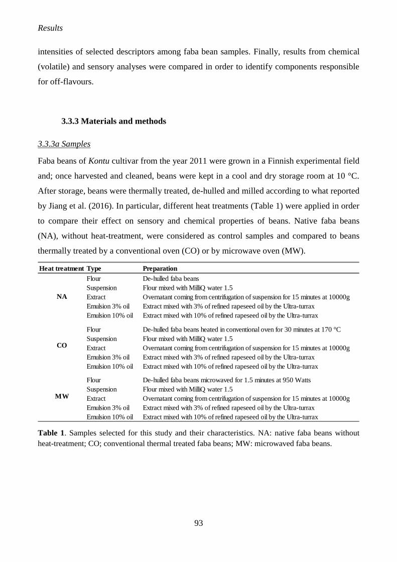
Results
93
intensities of selected descriptors among faba bean samples. Finally, results from chemical
(volatile) and sensory analyses were compared in order to identify components responsible
for off-flavours.
3.3.3 Materials and methods
3.3.3a Samples
Faba beans of Kontu cultivar from the year 2011 were grown in a Finnish experimental field
and; once harvested and cleaned, beans were kept in a cool and dry storage room at 10 °C.
After storage, beans were thermally treated, de-hulled and milled according to what reported
by Jiang et al. (2016). In particular, different heat treatments (Table 1) were applied in order
to compare their effect on sensory and chemical properties of beans. Native faba beans
(NA), without heat-treatment, were considered as control samples and compared to beans
thermally treated by a conventional oven (CO) or by microwave oven (MW).
Heat treatment Type Preparation
Flour De-hulled faba beans
Suspension Flour mixed with MilliQ water 1.5
Extract Overnatant coming from centrifugation of suspension for 15 minutes at 10000g
Emulsion 3% oil Extract mixed with 3% of refined rapeseed oil by the Ultra-turrax
Emulsion 10% oil Extract mixed with 10% of refined rapeseed oil by the Ultra-turrax
Flour De-hulled faba beans heated in conventional oven for 30 minutes at 170 °C
Suspension Flour mixed with MilliQ water 1.5
Extract Overnatant coming from centrifugation of suspension for 15 minutes at 10000g
Emulsion 3% oil Extract mixed with 3% of refined rapeseed oil by the Ultra-turrax
Emulsion 10% oil Extract mixed with 10% of refined rapeseed oil by the Ultra-turrax
Flour De-hulled faba beans microwaved for 1.5 minutes at 950 Watts
Suspension Flour mixed with MilliQ water 1.5
Extract Overnatant coming from centrifugation of suspension for 15 minutes at 10000g
Emulsion 3% oil Extract mixed with 3% of refined rapeseed oil by the Ultra-turrax
Emulsion 10% oil Extract mixed with 10% of refined rapeseed oil by the Ultra-turrax
NA
CO
MW
Table 1. Samples selected for this study and their characteristics. NA: native faba beans without
heat-treatment; CO; conventional thermal treated faba beans; MW: microwaved faba beans.
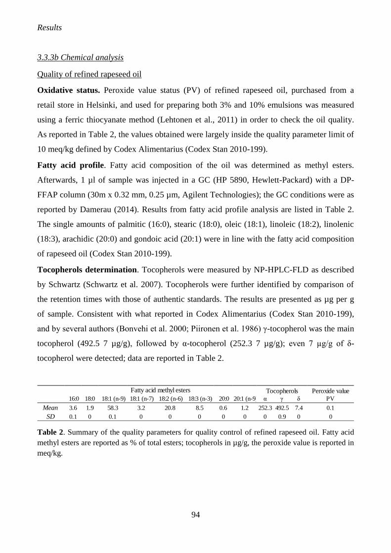
Results
94
3.3.3b Chemical analysis
Quality of refined rapeseed oil
Oxidative status. Peroxide value status (PV) of refined rapeseed oil, purchased from a
retail store in Helsinki, and used for preparing both 3% and 10% emulsions was measured
using a ferric thiocyanate method (Lehtonen et al., 2011) in order to check the oil quality.
As reported in Table 2, the values obtained were largely inside the quality parameter limit of
10 meq/kg defined by Codex Alimentarius (Codex Stan 2010-199).
Fatty acid profile. Fatty acid composition of the oil was determined as methyl esters.
Afterwards, 1 µl of sample was injected in a GC (HP 5890, Hewlett-Packard) with a DP-
FFAP column (30m x 0.32 mm, 0.25 µm, Agilent Technologies); the GC conditions were as
reported by Damerau (2014). Results from fatty acid profile analysis are listed in Table 2.
The single amounts of palmitic (16:0), stearic (18:0), oleic (18:1), linoleic (18:2), linolenic
(18:3), arachidic (20:0) and gondoic acid (20:1) were in line with the fatty acid composition
of rapeseed oil (Codex Stan 2010-199).
Tocopherols determination. Tocopherols were measured by NP-HPLC-FLD as described
by Schwartz (Schwartz et al. 2007). Tocopherols were further identified by comparison of
the retention times with those of authentic standards. The results are presented as µg per g
of sample. Consistent with what reported in Codex Alimentarius (Codex Stan 2010-199),
and by several authors (Bonvehi et al. 2000; Piironen et al. 1986) γ-tocopherol was the main
tocopherol (492.5 7 µg/g), followed by α-tocopherol (252.3 7 µg/g); even 7 µg/g of δ-
tocopherol were detected; data are reported in Table 2.
Peroxide value 16:0 18:0 18:1 (n-9) 18:1 (n-7) 18:2 (n-6) 18:3 (n-3) 20:0 20:1 (n-9) α γ δ PV
Mean 3.6 1.9 58.3 3.2 20.8 8.5 0.6 1.2 252.3 492.5 7.4 0.1
SD 0.1 0 0.1 0 0 0 0 0 0 0.9 0 0
Fatty acid methyl esters Tocopherols
Table 2. Summary of the quality parameters for quality control of refined rapeseed oil. Fatty acid
methyl esters are reported as % of total esters; tocopherols in µg/g, the peroxide value is reported in
meq/kg.
Results
95
Lipoxygenase activity determination
The LOX activity of flours from native beans and heat-treated beans was measured as
reported by Jiang et al. (2016). The method was modified from the the methods purposed by
Axelrod et al. (1981) and Gökmen (Gökmen et al. 2002)). For this spectrophotometric assay
0.5 g of NA, CO and MW flours were mixed with 29 ml of MQ-water, for 15 minutes. The
mixed samples were centrifuged for 10 minutes at 10000 g at room temperature, then the
supernatant was recollected and diluted 1:50. Sodium linoleate substrate solution (10 mM)
was prepared by mixing equal amount of Tween 20 and linoleic acid with 4 ml of MQ-water
and, in order to clarify the solution, 30 µl of NaOH (1 N) was added. For measuring the
lipoxygenase activity, reaction was made adding 200 µl of substrate solution and 200 µl of
extract to 2.6 ml of sodium phosphate buffer (pH 6). After incubating the mixture for 3
minutes at 25 °C, the reaction was stopped by adding 3 ml of NAOH (0.1 N) to the mixture.
Absorbance was measured at wavelength of 234nm (Lamba 25 UV/Vis, Perkin Elmer Inc.,
USA). Results were then calculated with molar absorptivity value of conjugated dienes
(ɛ=26000 l/mol cm).
3.3.3c Volatile compounds analysis
Volatile compounds present in the samples were analysed by HS-SPME-GC-MS. The HS-
SPME–GC–MS method was developed modifying a previously reported method (Damerau
et al., 2014).
Optimization of the method
Prior to GC analysis for identifying the key aroma-active compounds, optimization of the
SPME method to extract the maximum number of the most aroma-active compounds from
the sample was carried out. The optimization of the method was carried out using faba
beans samples from Kontu cultivar, harvest year 2011. Flours were prepared from native
(NA, no heat treatment), conventionally oven heated (CO) and microwave (MW) treated
beans and studied as: a) flour, b) suspension (water), c) extract, produced as reported in
Samples’s paragraph. Samples were analysed in duplicates.
Results
96
Volatile compounds were analysed using an HS-SPME injector (combiPAL, CTC
Analytics, USA), with a divinylbenzene/carboxen/polydimethylsiloxane fiber
(DVB/CAR/PDMS-fiber, 50/30 µm film thickness; Supelco, USA) and a
carboxen/polydimethylsiloxane fiber (CAR/PDMS-fiber 85 µm film thickness; Supelco,
USA). The SPME fibers were conditioned before the first use according to the instructions
of the supplier. The SPME was coupled to a GC (HP 6890 series, Agilent Technologies
Inc., Wilmington, DE, USA) with a MS detector (Agilent 5973 Network, Agilent
Technologies Inc., Wilmington, DE, USA). The GC was equipped with a capillary column
SPB-624 (30 m x 0.25 mm i.d., 1.4 µm film thickness; Supelco, USA). The extraction times
tested were 30 and 60 minutes. The instrument and measuring parameters were as reported
in section Optimized method for HS-SPME-GC-MS.
Optimized method for HS-SPME-GC-MS
Different fibers were selected for different models: DVB/CAR/PDMS-fiber was used for
liquid samples (suspensions, extracts, emulsions) while CAR/PDMS was selected for
analysing flours. The extraction time was fixed at 60 minutes and the temperature was set at
50 °C. The fiber was then desorbed for 10 min at 250 °C in the injection port of the GC
operating in splitless mode. The GC operating conditions were the following: helium flow
rate 0.7 mL/min; oven temperature increasing steps: 40 °C for 5 min, then increased by 5
°C/min to 200 °C and held at 200 °C for 10 min. The ionisation energy of MS was 70 eV
and the range of the scan was from 50 to 300 amu. The match between compounds mass
spectra and the database Wiley 7N was used for the identification of volatiles (Wiley
Registry™ of Mass Spectral Data, 7th Edition, USA). Total ion counts were used for
quantifying the amounts of compounds. Peak areas of six and three volatiles of two
reference materials, blueberry oatmeal cookies and vanilla soymilk, for flours and liquid
samples respectively, were used for monitoring the performance of the HS-SPME–GC–MS.
All measurements were done over a time period of 4 weeks. Samples were analysed in
triplicates.
Results
97
3.3.3d Sensory analysis
Samples were evaluated with Generic Descriptive analysis (GDA) (Lawless and Heymann,
2010; Murray et al., 2001). The method provides information about the qualitative as well
as the quantitative characteristics of samples. It is widely used for obtaining detailed
description of the appearance, aroma, flavour, and texture of food products.
Panel members (n=9, 7 females, 2 males, age from 21 to 44; students and employees of the
University of Helsinki) served as panellists. Study protocol followed the ethical guidelines
of the sensory laboratory, approved by the University of Helsinki Ethical Review Board in
the Humanities and Social and Behavioural Sciences. A written informed consent was
obtained from each participant before they entered the screening phase.
Panellists were screened for their sense of smell with Sniffin’ Sticks Screening (SSS), in
which odour of 12 felt-tip pens (sticks) is to be identified among four alternative
descriptions given for each stick. The number of correct identifications of odorants define
the capacity (Hummel et al., 1997). Values of 11-12 are considered normal, while 10 or less
need a further examination of the olfactory performance; all the assessors obtained 11-12.
The procedure of selecting optimal descriptors, references and appropriate scales, training
and evaluation followed the practical principles of GDA as described by Lawless and
Heymann (2010). At the beginning of the experiment, panellists worked individually trying
to describe the samples using their own terms: after that, the panel leader guided the
discussion through which the attributes were selected. The training phase consisted of three
one-hour sessions during which each panellist received all samples tobe evaluated; the panel
decided whether descriptors were redundant and should be removed from the list or if there
were terms that should be added. The training sessions included familiarization with the
attributes and references selection: assessors identified possible reference standards on
which the rating of the generated attributes was based. Finally, eight olfactory attributes
were chosen, paired to their references (Table 3).
Sensory profiling was performed on the 15 samples reported in Table 1. The panelists
received seven or eight samples at a time, (15 ± 0.5g) placed in 50 ml dark container closed
with plastic cap. Samples were presented coded with three-digit numbers; each panelist
worked individually in a panel room, inside singular closed booth, in white light condition.
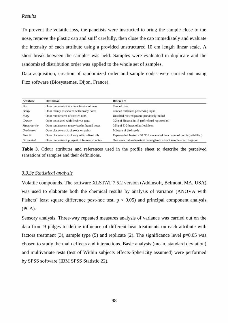
Results
98
To prevent the volatile loss, the panelists were instructed to bring the sample close to the
nose, remove the plastic cap and sniff carefully, then close the cap immediately and evaluate
the intensity of each attribute using a provided unstructured 10 cm length linear scale. A
short break between the samples was held. Samples were evaluated in duplicate and the
randomized distribution order was applied to the whole set of samples.
Data acquisition, creation of randomized order and sample codes were carried out using
Fizz software (Biosystemes, Dijon, France).
Attribute Definition Reference
Pea Odor reminescent or characteristic of peas Canned peas
Beany Odor mainly associated with beany notes Canned red beans preserving liquid
Nutty Odor reminescent of roasted nuts Unsalted roasted peanut previously milled
Grassy Odor associated with fresh vut grass 0.2 g of Hexanal in 15 g of refined rapeseed oil
Musty/earthy Odor reminescent musty/earthy/humid notes 0.5 g of Z-2-hexenol in fresh loam
Grain/seed Odor characteristic of seeds or grains Mixture of bird seeds
Rancid Odor characteristic of very old/oxidized oils Rapeseed oil heated a 60 °C for one week in an opened bottle (half-filled)
Fermented Odor reminescent pungent of fermented notes One week old undernatant coming from extract samples centrifugation
Table 3. Odour attributes and references used in the profile sheet to describe the perceived
sensations of samples and their definitions.
3.3.3e Statistical analysis
Volatile compounds. The software XLSTAT 7.5.2 version (Addinsoft, Belmont, MA, USA)
was used to elaborate both the chemical results by analysis of variance (ANOVA with
Fishers’ least square difference post-hoc test, p < 0.05) and principal component analysis
(PCA).
Sensory analysis. Three-way repeated measures analysis of variance was carried out on the
data from 9 judges to define influence of different heat treatments on each attribute with
factors treatment (3), sample type (5) and replicate (2). The significance level p=0.05 was
chosen to study the main effects and interactions. Basic analysis (mean, standard deviation)
and multivariate tests (test of Within subjects effects-Sphericity assumed) were performed
by SPSS software (IBM SPSS Statistic 22).
Results
99
3.3.4 Results and discussion
3.3.4a Lipoxygenase activity determination
Considering the measurement of LOX activity, both the heat treatments reduced the
enzymatic activity. The enzymatic activity in NA sample was 336.8 ± 7.9 µmol of
hydroperoxides/g of sample/min. The strongest heat-treatment, in terms of LOX activity
reduction, was the conventional thermal treatment. In fact, in CO flour, the enzyme activity
was reduced by 81.1% (63.8 ± 5.7), while in MW flour the lipoxygenase activity was
reduced by 71.58% (95.7 ± 10.8) with respect to the native sample. As a result, the heat
treatments were not strong enough for switching off completely the LOX activity. Thus, the
potential of formation of compounds lypoxygenase-catalysed and responsible for off-
flavour was reduced but not effectively eliminated.
3.3.4b Volatile compounds analysis
Fiber comparison. After testing CAR/PDMS and DVB/CAR/PDMS fibers on liquid and
solid samples, the first was selected for the analysis of flours, while the latter was used for
obtaining the volatile profile of liquid models. The quantification of 35 compounds
tentatively identified in the volatile profile of flour and extract from NA Finnish faba beans
is reported in Figure 1, highlighting that while CAR/PDMS allows to collect greater
amounts of volatile compounds in solid samples from flour samples, CAR/DVB/PDMS was
more effective in collecting from liquid ones. Taking into account many of the volatiles
detected, it can be seen that how the hexanal in flour samples is better detect if the
CAR/PDMS fiber is used; on the other hands, octen-3-ol, in extract, gave higher responses
with the use of DVB/CAR/PDMS; the same behaviour could be described for limonene.
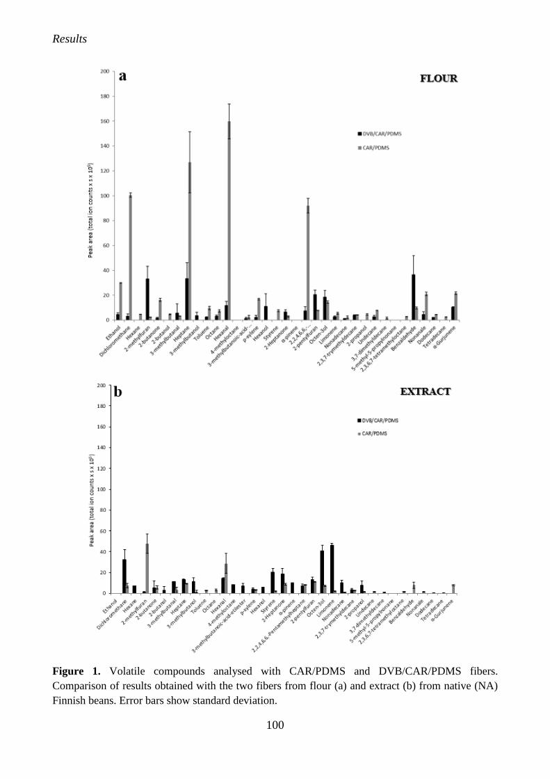
Results
100
Figure 1. Volatile compounds analysed with CAR/PDMS and DVB/CAR/PDMS fibers.
Comparison of results obtained with the two fibers from flour (a) and extract (b) from native (NA)
Finnish beans. Error bars show standard deviation.
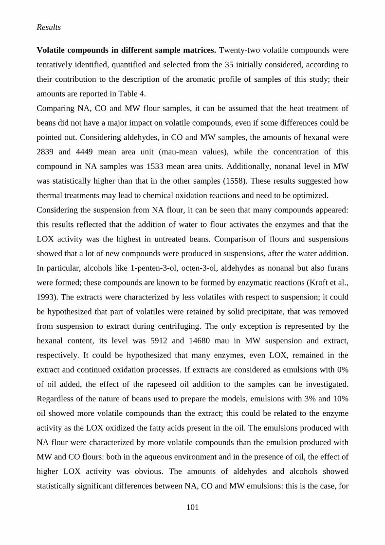
Results
101
Volatile compounds in different sample matrices. Twenty-two volatile compounds were
tentatively identified, quantified and selected from the 35 initially considered, according to
their contribution to the description of the aromatic profile of samples of this study; their
amounts are reported in Table 4.
Comparing NA, CO and MW flour samples, it can be assumed that the heat treatment of
beans did not have a major impact on volatile compounds, even if some differences could be
pointed out. Considering aldehydes, in CO and MW samples, the amounts of hexanal were
2839 and 4449 mean area unit (mau-mean values), while the concentration of this
compound in NA samples was 1533 mean area units. Additionally, nonanal level in MW
was statistically higher than that in the other samples (1558). These results suggested how
thermal treatments may lead to chemical oxidation reactions and need to be optimized.
Considering the suspension from NA flour, it can be seen that many compounds appeared:
this results reflected that the addition of water to flour activates the enzymes and that the
LOX activity was the highest in untreated beans. Comparison of flours and suspensions
showed that a lot of new compounds were produced in suspensions, after the water addition.
In particular, alcohols like 1-penten-3-ol, octen-3-ol, aldehydes as nonanal but also furans
were formed; these compounds are known to be formed by enzymatic reactions (Kroft et al.,
1993). The extracts were characterized by less volatiles with respect to suspension; it could
be hypothesized that part of volatiles were retained by solid precipitate, that was removed
from suspension to extract during centrifuging. The only exception is represented by the
hexanal content, its level was 5912 and 14680 mau in MW suspension and extract,
respectively. It could be hypothesized that many enzymes, even LOX, remained in the
extract and continued oxidation processes. If extracts are considered as emulsions with 0%
of oil added, the effect of the rapeseed oil addition to the samples can be investigated.
Regardless of the nature of beans used to prepare the models, emulsions with 3% and 10%
oil showed more volatile compounds than the extract; this could be related to the enzyme
activity as the LOX oxidized the fatty acids present in the oil. The emulsions produced with
NA flour were characterized by more volatile compounds than the emulsion produced with
MW and CO flours: both in the aqueous environment and in the presence of oil, the effect of
higher LOX activity was obvious. The amounts of aldehydes and alcohols showed
statistically significant differences between NA, CO and MW emulsions: this is the case, for
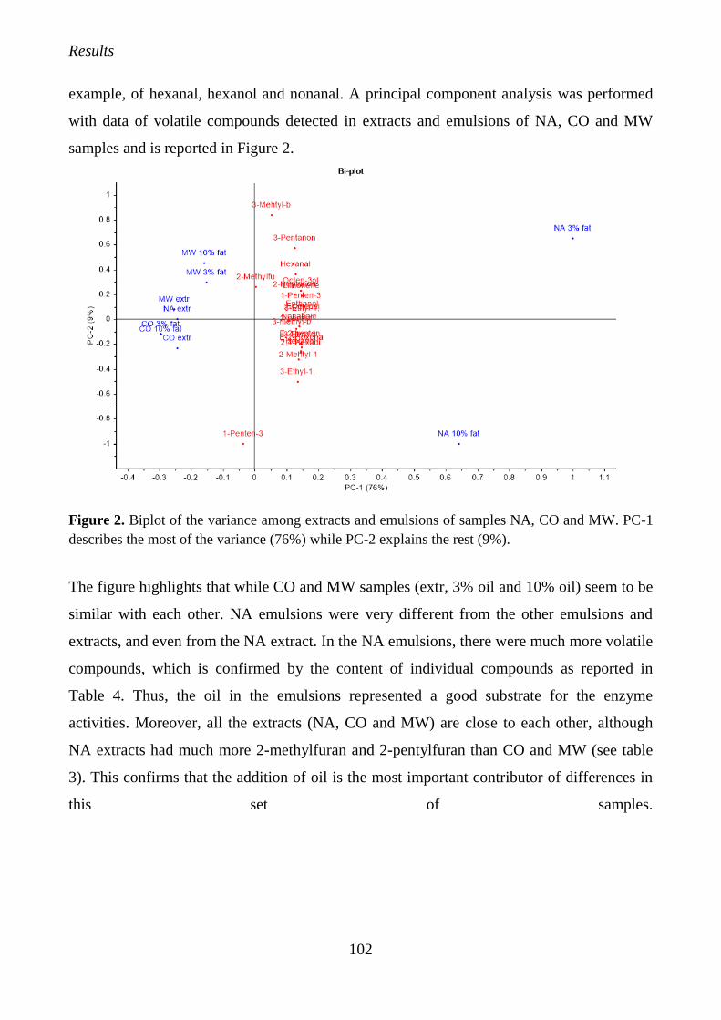
Results
102
example, of hexanal, hexanol and nonanal. A principal component analysis was performed
with data of volatile compounds detected in extracts and emulsions of NA, CO and MW
samples and is reported in Figure 2.
Figure 2. Biplot of the variance among extracts and emulsions of samples NA, CO and MW. PC-1
describes the most of the variance (76%) while PC-2 explains the rest (9%).
The figure highlights that while CO and MW samples (extr, 3% oil and 10% oil) seem to be
similar with each other. NA emulsions were very different from the other emulsions and
extracts, and even from the NA extract. In the NA emulsions, there were much more volatile
compounds, which is confirmed by the content of individual compounds as reported in
Table 4. Thus, the oil in the emulsions represented a good substrate for the enzyme
activities. Moreover, all the extracts (NA, CO and MW) are close to each other, although
NA extracts had much more 2-methylfuran and 2-pentylfuran than CO and MW (see table
3). This confirms that the addition of oil is the most important contributor of differences in
this set of samples.
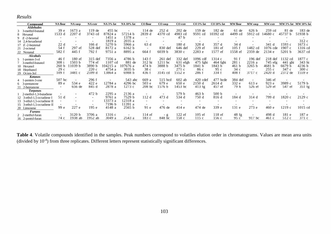
Results
103
CompoundAldehydes
3 3-methyl-butanal 39 e 1673 a 119 de 455 bc 114 de 252 d 202 de 159 de 182 de 61 de 626 b 259 cd 81 de 183 de 8 Hexanal 1533 d 2207 d 3743 cd 87824 a 57214 b 2839 d 4370 cd 4983 cd 9591 cd 10392 cd 4499 cd 5912 cd 14680 c 45737 b 51938 b 9 E -2-hexenal 1451 a 1378 a 47 b 14 2,4-hexadienal 1819 a 2035 a 312 c 17 E -2-heptenal 22 d 166 d 5270 b 5966 a 63 d 180 d 328 d 357 d 34 d 341 d 1593 c 1673 c 21 2-octenal 54 f 297 ef 528 def 8172 a 6162 b - 830 def 646 def 229 ef 181 ef 105 f 1482 cd 1076 cde 1907 c 1316 cd
22 Nonanal 582 f 445 f 792 f 9751 a 8895 a 664 f 6039 b 3830 c 2283 e 1577 ef 1558 ef 2359 de 2134 e 5201 b 3637 cd Alcohols
5 1-penten-3-ol 46 f 180 ef 315 def 7356 a 4786 b 143 f 261 def 332 def 1096 cdf 1314 c 91 f 196 def 218 def 1132 cd 1877 c 7 3-methyl-butanol 308 i 1503 b 774 ef 1107 cd 881 de 312 hi 1211 bc 631 efgh 475 fghi 464 fghi 281 i 2216 a 745 efg 441 ghi 343 hi 10 Hexanol 260 b 11039 b 3890 b 104215 a 107676 a 474 b 3888 b 3475 b 1841 b 1843 b 461 b 3265 b 4681 b 6679 b 4236 b 18 Hepthanol 29 c 220 c 4754 a 3035 b 38 c 271 c 86 c 95 c 34 c 255 c 347 c 300 c 19 Octen-3ol 109 f 3481 c 2599 d 13864 a 6988 b 436 f 3145 cd 1552 e 286 f 334 f 408 f 3717 c 2420 d 2372 de 1559 e
Ketones4 1-penten-3-one 507 bcd 296 f 543 abc 669 a 515 bcd 602 ab 420 cdef 477 bcde 384 def 346 ef 6 3-pentanone 89 e 534 e 422 e 12784 a 4296 bc 503 e 679 e 650 e 2150 d 2614 d 332 e 613 e 923 e 3989 c 5179 b 11 2-heptanone 656 de 845 d 2878 a 1273 c 208 bc 1576 b 1453 bc 413 fg 457 ef 79 h 526 ef 529 ef 547 ef 351 fg
Terpenes1 2-methyl-1,3-butadiene 472 b 2295 a 2136 a 579 b 463 b 500 b 12 3-ethyl-1,5-octadiene I 51 d 9761 a 7529 b 112 d 473 d 534 d 750 d 816 d 184 d 314 d 799 d 1820 c 2129 c 13 3-ethyl-1,5-octadiene II 13373 a 12318 a 15 3-ethyl-1,5-octadiene III 7196 b 11391 a 20 Limonene 99 e 227 e 195 e 4148 a 2565 b 91 e 476 de 414 e 474 de 339 e 131 e 273 e 460 e 1219 c 1015 cd
Furans2 2-methyl-furan 3120 b 3706 a 1316 c 114 ef - g 122 ef 105 ef 118 ef 48 fg 498 d 181 e 187 e 16 2-pentyl-furan 74 c 1938 ab 1952 ab 3049 a 2543 a 183 c 848 bc 158 c 115 c 156 c 95 c 917 bc 461 c 512 c 371 c
-
-
- - - - - -
- -
- - - - - -
- - - - -
- - - - -
-
- - -
MW flour MW susp MW extr MW 3% fat MW 10% fat
- - - - -
- - - - - - - -
-
-
- -
- -
CO flour CO susp CO extr CO 3% fat CO 10% fat
- - - -
- - - - - - - - -
- - -
-
-
- -
-
NA 10% fat
- -
NA flour NA susp NA extr NA 3% fat
-
- - - -
Table 4. Volatile compounds identified in the samples. Peak numbers correspond to volatiles elution order in chromatograms. Values are mean area units
(divided by 10-4) from three replicates. Different letters represent statistically significant differences.
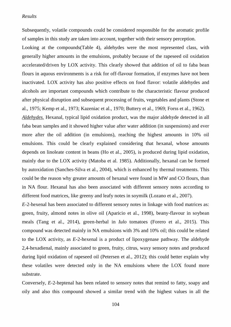
Results
104
Subsequently, volatile compounds could be considered responsible for the aromatic profile
of samples in this study are taken into account, together with their sensory perception.
Looking at the compounds(Table 4), aldehydes were the most represented class, with
generally higher amounts in the emulsions, probably because of the rapeseed oil oxidation
accelerated/driven by LOX activity. This clearly showed that addition of oil to faba bean
flours in aquous environments is a risk for off-flavour formation, if enzymes have not been
inactivated. LOX activity has also positive effects on food flavor: volatile aldehydes and
alcohols are important compounds which contribute to the characteristic flavour produced
after physical disruption and subsequent processing of fruits, vegetables and plants (Stone et
al., 1975; Kemp et al., 1973; Kazeniac et al., 1970; Buttery et al., 1969; Forss et al., 1962).
Aldehydes. Hexanal, typical lipid oxidation product, was the major aldehyde detected in all
faba bean samples and it showed higher value after water addition (in suspensions) and ever
more after the oil addition (in emulsions), reaching the highest amounts in 10% oil
emulsions. This could be clearly explained considering that hexanal, whose amounts
depends on linoleate content in beans (Ho et al., 2005), is produced during lipid oxidation,
mainly due to the LOX activity (Matoba et al. 1985). Additionally, hexanal can be formed
by autoxidation (Sanches-Silva et al., 2004), which is enhanced by thermal treatments. This
could be the reason why greater amounts of hexanal were found in MW and CO flours, than
in NA flour. Hexanal has also been associated with different sensory notes according to
different food matrices, like greeny and leafy notes in soymilk (Lozano et al., 2007).
E-2-hexenal has been associated to different sensory notes in linkage with food matrices as:
green, fruity, almond notes in olive oil (Aparicio et al., 1998), beany-flavour in soybean
meals (Tang et al., 2014), green-herbal in Iulo tomatoes (Forero et al., 2015). This
compound was detected mainly in NA emulsions with 3% and 10% oil; this could be related
to the LOX activity, as E-2-hexenal is a product of lipoxygenase pathway. The aldehyde
2,4-hexadienal, mainly associated to green, fruity, citrus, waxy sensory notes and produced
during lipid oxidation of rapeseed oil (Petersen et al., 2012); this could better explain why
these volatiles were detected only in the NA emulsions where the LOX found more
substrate.
Conversely, E-2-heptenal has been related to sensory notes that remind to fatty, soapy and
oily and also this compound showed a similar trend with the highest values in all the
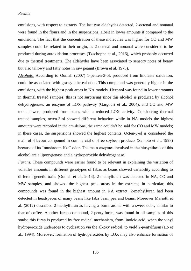
Results
105
emulsions, with respect to extracts. The last two aldehydes detected, 2-octenal and nonanal
were found in the flours and in the suspensions, albeit in lower amounts if compared to the
emulsions. The fact that the concentration of these molecules was higher for CO and MW
samples could be related to their origin, as 2-octenal and nonanal were considered to be
produced during autoxidation processes (Tzschoppe et al., 2016), which probably occurred
due to thermal treatments. The aldehydes have been associated to sensory notes of beany
but also tallowy and fatty notes in raw peanut (Brown et al. 1973).
Alcohols. According to Oomah (2007) 1-penten-3-ol, produced from linoleate oxidation,
could be associated with grassy ethereal odor. This compound was generally higher in the
emulsions, with the highest peak areas in NA models. Hexanol was found in lower amounts
in thermal treated samples: this is not surprising since this alcohol is produced by alcohol
dehydrogenase, an enzyme of LOX pathway (Gargouri et al., 2004), and CO and MW
models were produced from beans with a reduced LOX activity. Considering thermal
treated samples, octen-3-ol showed different behavior: while in NA models the highest
amounts were recorded in the emulsions, the same couldn’t be said for CO and MW models;
in these cases, the suspensions showed the highest contents. Octen-3-ol is considered the
main off-flavour compound in commercial oil-free soybean products (Samoto et al., 1998)
because of its “mushroom-like” odor. The main enzymes involved in the biosynthesis of this
alcohol are a lipoxygenase and a hydroperoxide dehydrogenase.
Furans. These compounds were earlier found to be relevant in explaining the variation of
volatiles amounts in different genotypes of fabas as beans showed variability according to
different genetic traits (Oomah et al., 2014). 2-methylfuran was detected in NA, CO and
MW samples, and showed the highest peak areas in the extracts; in particular, this
compounds was found in the highest amount in NA extract. 2-methylfuran had been
detected in headspaces of many beans like faba bean, pea and beans. Moreover Mariotti et
al. (2012) described 2-methylfuran as having a burnt aroma with a sweet odor, similar to
that of coffee. Another furan compound, 2-pentylfuran, was found in all samples of this
study; this furan is produced by free radical mechanism, from linoleic acid, when the vinyl
hydroperoxide undergoes to cyclization via the alkoxy radical, to yield 2-pentylfuran (Ho et
al., 1994). Moreover, formation of hydroperoxides by LOX may also enhance formation of
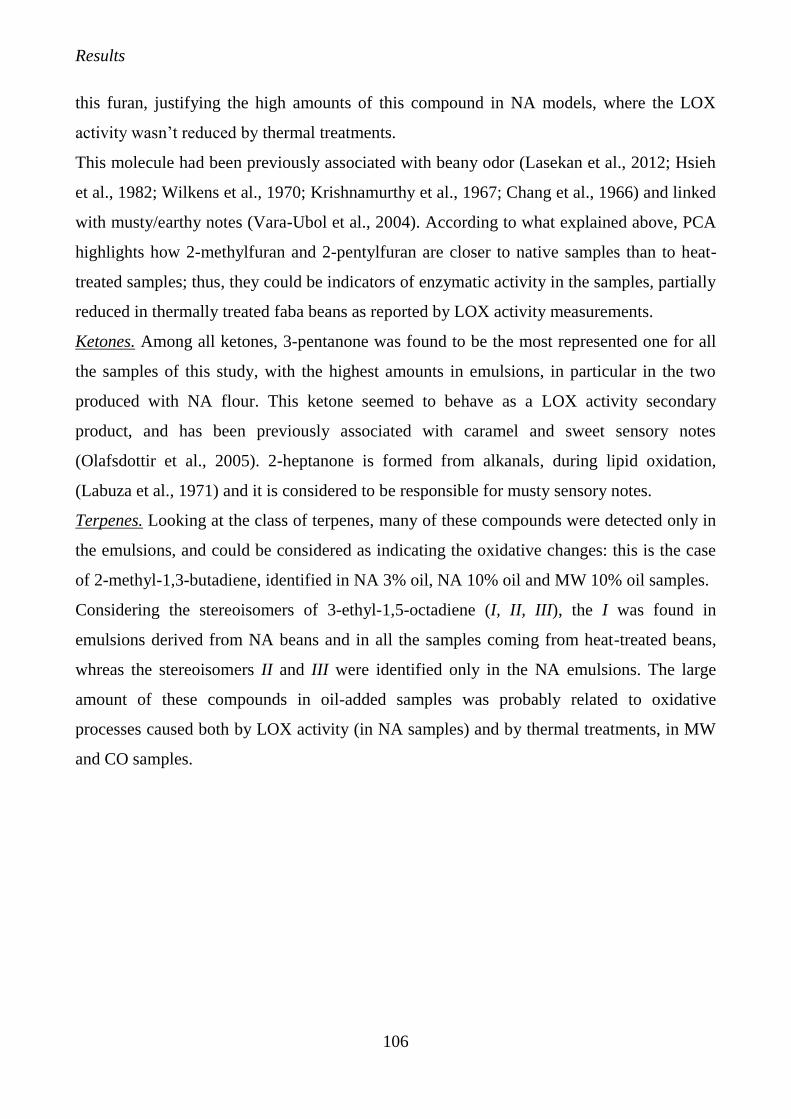
Results
106
this furan, justifying the high amounts of this compound in NA models, where the LOX
activity wasn’t reduced by thermal treatments.
This molecule had been previously associated with beany odor (Lasekan et al., 2012; Hsieh
et al., 1982; Wilkens et al., 1970; Krishnamurthy et al., 1967; Chang et al., 1966) and linked
with musty/earthy notes (Vara-Ubol et al., 2004). According to what explained above, PCA
highlights how 2-methylfuran and 2-pentylfuran are closer to native samples than to heat-
treated samples; thus, they could be indicators of enzymatic activity in the samples, partially
reduced in thermally treated faba beans as reported by LOX activity measurements.
Ketones. Among all ketones, 3-pentanone was found to be the most represented one for all
the samples of this study, with the highest amounts in emulsions, in particular in the two
produced with NA flour. This ketone seemed to behave as a LOX activity secondary
product, and has been previously associated with caramel and sweet sensory notes
(Olafsdottir et al., 2005). 2-heptanone is formed from alkanals, during lipid oxidation,
(Labuza et al., 1971) and it is considered to be responsible for musty sensory notes.
Terpenes. Looking at the class of terpenes, many of these compounds were detected only in
the emulsions, and could be considered as indicating the oxidative changes: this is the case
of 2-methyl-1,3-butadiene, identified in NA 3% oil, NA 10% oil and MW 10% oil samples.
Considering the stereoisomers of 3-ethyl-1,5-octadiene (I, II, III), the I was found in
emulsions derived from NA beans and in all the samples coming from heat-treated beans,
whreas the stereoisomers II and III were identified only in the NA emulsions. The large
amount of these compounds in oil-added samples was probably related to oxidative
processes caused both by LOX activity (in NA samples) and by thermal treatments, in MW
and CO samples.
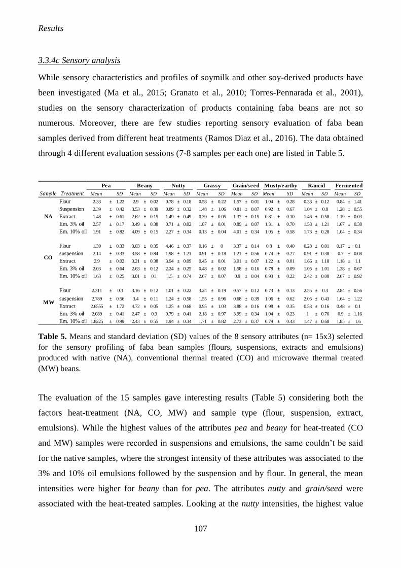
Results
107
3.3.4c Sensory analysis
While sensory characteristics and profiles of soymilk and other soy-derived products have
been investigated (Ma et al., 2015; Granato et al., 2010; Torres-Pennarada et al., 2001),
studies on the sensory characterization of products containing faba beans are not so
numerous. Moreover, there are few studies reporting sensory evaluation of faba bean
samples derived from different heat treatments (Ramos Diaz et al., 2016). The data obtained
through 4 different evaluation sessions (7-8 samples per each one) are listed in Table 5.
Mean SD Mean SD Mean SD Mean SD Mean SD Mean SD Mean SD Mean SD
Flour 2.33 ± 1.22 2.9 ± 0.02 0.78 ± 0.18 0.58 ± 0.22 1.57 ± 0.01 1.04 ± 0.28 0.33 ± 0.12 0.84 ± 1.41
Suspension 2.39 ± 0.42 3.53 ± 0.39 0.89 ± 0.32 1.48 ± 1.06 0.81 ± 0.07 0.92 ± 0.67 1.04 ± 0.8 1.28 ± 0.55
Extract 1.48 ± 0.61 2.62 ± 0.15 1.49 ± 0.49 0.39 ± 0.05 1.37 ± 0.15 0.81 ± 0.10 1.46 ± 0.58 1.19 ± 0.03
Em. 3% oil 2.57 ± 0.17 3.49 ± 0.38 0.71 ± 0.02 1.87 ± 0.01 0.89 ± 0.07 1.31 ± 0.70 1.58 ± 1.21 1.67 ± 0.38
Em. 10% oil 1.91 ± 0.82 4.09 ± 0.15 2.27 ± 0.34 0.13 ± 0.04 4.01 ± 0.34 1.05 ± 0.58 1.73 ± 0.28 1.04 ± 0.34
Flour 1.39 ± 0.33 3.03 ± 0.35 4.46 ± 0.37 0.16 ± 0 3.37 ± 0.14 0.8 ± 0.40 0.28 ± 0.01 0.17 ± 0.1
suspension 2.14 ± 0.33 3.58 ± 0.84 1.98 ± 1.21 0.91 ± 0.18 1.21 ± 0.56 0.74 ± 0.27 0.91 ± 0.38 0.7 ± 0.08
Extract 2.9 ± 0.02 3.21 ± 0.38 3.94 ± 0.09 0.45 ± 0.01 3.01 ± 0.07 1.22 ± 0.01 1.66 ± 1.18 1.18 ± 1.1
Em. 3% oil 2.03 ± 0.64 2.63 ± 0.12 2.24 ± 0.25 0.48 ± 0.02 1.58 ± 0.16 0.78 ± 0.09 1.05 ± 1.01 1.38 ± 0.67
Em. 10% oil 1.63 ± 0.25 3.01 ± 0.1 1.5 ± 0.74 2.67 ± 0.07 0.9 ± 0.04 0.93 ± 0.22 2.42 ± 0.08 2.67 ± 0.92
Flour 2.311 ± 0.3 3.16 ± 0.12 1.01 ± 0.22 3.24 ± 0.19 0.57 ± 0.12 0.73 ± 0.13 2.55 ± 0.3 2.84 ± 0.56
suspension 2.789 ± 0.56 3.4 ± 0.11 1.24 ± 0.58 1.55 ± 0.96 0.68 ± 0.39 1.06 ± 0.62 2.05 ± 0.43 1.64 ± 1.22
Extract 2.6555 ± 1.72 4.72 ± 0.05 1.25 ± 0.68 0.95 ± 1.03 3.88 ± 0.16 0.98 ± 0.35 0.53 ± 0.16 0.48 ± 0.1
Em. 3% oil 2.089 ± 0.41 2.47 ± 0.3 0.79 ± 0.41 2.18 ± 0.97 3.99 ± 0.34 1.04 ± 0.23 1 ± 0.76 0.9 ± 1.16
Em. 10% oil 1.8225 ± 0.99 2.43 ± 0.55 1.94 ± 0.34 1.71 ± 0.82 2.73 ± 0.37 0.79 ± 0.43 1.47 ± 0.68 1.85 ± 1.6
Rancid Fermented
NA
CO
MW
Sample Treatment
Pea Beany Nutty Grassy Grain/seed Musty/earthy
Table 5. Means and standard deviation (SD) values of the 8 sensory attributes (n= 15x3) selected
for the sensory profiling of faba bean samples (flours, suspensions, extracts and emulsions)
produced with native (NA), conventional thermal treated (CO) and microwave thermal treated
(MW) beans.
The evaluation of the 15 samples gave interesting results (Table 5) considering both the
factors heat-treatment (NA, CO, MW) and sample type (flour, suspension, extract,
emulsions). While the highest values of the attributes pea and beany for heat-treated (CO
and MW) samples were recorded in suspensions and emulsions, the same couldn’t be said
for the native samples, where the strongest intensity of these attributes was associated to the
3% and 10% oil emulsions followed by the suspension and by flour. In general, the mean
intensities were higher for beany than for pea. The attributes nutty and grain/seed were
associated with the heat-treated samples. Looking at the nutty intensities, the highest value
Results
108
was for the CO samples, especially in flour, followed by extract and 3% oil emulsion. For
MW samples, intensities seemed to be lower. The highest intensity was observed in 10% oil
emulsion sample with mean value of 2 (1.94 ±0.34). The mean intensities of this attribute in
NA samples were really low, with the only exception of the 10% oil emulsion. A similar
perception regards grain/seed. In fact, the intensities of this attribute in NA samples were
low, except for the 10% oil emulsion; anyhow, thermal treated samples showed higher
intensities of this attribute. In particular, while for conventional thermal treated models the
highest values of grain/seed were associated both with flour and extract (3.37 ±0.14 and
3.01±0.07 respectively), for the microwaved samples this descriptor had the highest
intensities in extract but also in 3% and 10% oil emulsions. Grassy was always reported
with very low intensities but seems to be mainly associated with emulsions, the 3% oil for
MW and NA beans and the 10% oil for CO. The intensity of attributes considered as
negative were generally low. Considering musty/earthy, the ranges of values were 0.81-
1.31, 0.74-1.22 and 0.73-1.06 for NA, CO and MW models respectively; this descriptor
seemed not to have statistical relevance in discriminating among different heat treated
samples. A similar trend characterized fermented and rancid, that showed the highest
intensities in NA and CO 10 % oil and in MW flour.
In order to describe the significant differences eventually existing among the samples, a
multifactorial analysis of variance was carried out (Table 6). The analysis of variance was
performed for 7 of the 8 attributes: pea, nutty, grassy, grain/seed, musty/earthy, rancid,
fermented.
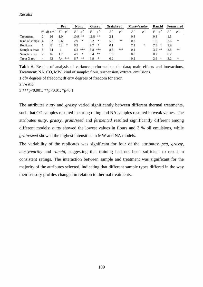
Results
109
df df err1
F2
p3
F2
p3
F2
p3
F2
p3
F2
p3
F2
p3
F2
p3
Treatment 2 16 1.0 10.9 ** 11.8 ** 2.1 0.3 0.3 1.3
Kind of sample 4 32 0.6 2.9 * 3.2 * 5.3 ** 0.2 1.6 2.6 *
Replicate 1 8 13 * 0.3 9.7 * 0.1 7.1 * 7.3 * 1.9
Sample x treat 8 64 1 6.2 *** 5.8 *** 8.3 *** 0.4 3.2 ** 3.8 **
Sample x rep 2 16 1.7 4.7 * 9.4 ** 1.6 0.0 0.2 0.2
Treat X rep 4 32 7.4 *** 6.7 ** 3.9 * 0.2 0.2 2.9 * 3.2 *
Pea Musty/earthy Rancid FermentedNutty Grassy Grain/seed
Table 6. Results of analysis of variance performed on the data; main effects and interactions.
Treatment: NA, CO, MW; kind of sample: flour, suspension, extract, emulsions.
1 df= degrees of freedom; df err= degrees of freedom for error.
2 F-ratio
3 ***p<0.001; **p<0.01; *p<0.1
The attributes nutty and grassy varied significantly between different thermal treatments,
such that CO samples resulted in strong rating and NA samples resulted in weak values. The
attributes nutty, grassy, grain/seed and fermented resulted significantly different among
different models: nutty showed the lowest values in flours and 3 % oil emulsions, while
grain/seed showed the highest intensities in MW and NA models.
The variability of the replicates was significant for four of the attributes: pea, grassy,
musty/earthy and rancid, suggesting that training had not been sufficient to result in
consistent ratings. The interaction between sample and treatment was significant for the
majority of the attributes selected, indicating that different sample types differed in the way
their sensory profiles changed in relation to thermal treatments.
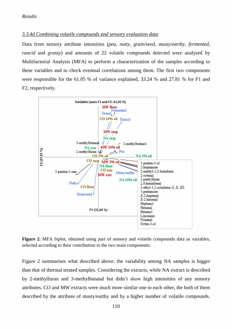
Results
110
3.3.4d Combining volatile compounds and sensory evaluation data
Data from sensory attribute intensities (pea, nutty, grain/seed, musty/earthy, fermented,
rancid and grassy) and amounts of 22 volatile compounds detected were analysed by
Multifactorial Analysis (MFA) to perform a characterization of the samples according to
these variables and to check eventual correlations among them. The first two components
were responsible for the 61.05 % of variance explained, 33.24 % and 27.81 % for F1 and
F2, respectively.
Figure 2. MFA biplot, obtained using part of sensory and volatile compounds data as variables,
selected according to their contribution to the two main components.
Figure 2 summarises what described above: the variability among NA samples is bigger
than that of thermal treated samples. Considering the extracts, while NA extract is described
by 2-methylfuran and 3-methylbutanal but didn’t show high intensities of any sensory
attributes. CO and MW extracts were much more similar one to each other, the both of them
described by the attribute of musty/earthy and by a higher number of volatile compounds.
Results
111
The CO flour was close to the attributes of nutty and grain/seed, probably because of the
effect of heat treatment, together with CO susp and emulsion CO 3% oil, while MW flour
was characterized by the attributes of fermented, grassy and rancid. Additionally, the
attributes grassy and fermented were positively correlated (r = 0.78) while the attribute nutty
resulted to be positively correlated with 1-penten-3-one (r = 0.64). The most of the volatile
compounds detected in samples in this study appeared to be close to the emulsions produced
using native faba bean flour (emulsions NA 3% and 10% oil): this is not surprising as these
compounds are generated during LOX activity, which was reported to be at its maximum in
NA beans. For example, among aldehydes produced during oxidative processes, 2-octenal,
associated with sensory notes of beany and tallow, resulted to be positively correlated with
the attribute of musty/earthy.
3.3.5 Conclusions
At present, there are no scientific studies that have analysed both volatile compound
amounts and sensory attribute intensities to characterize different faba bean samples.
Starting from beans, different models were produce: in particular, beans were thermally
treated with a conventional oven or with a microwave oven, then de-hulled; native untreated
beans were analysed as control samples. After that, different models were prepared, in order
to reproduce different uses of this bean in common food models: suspensions (with water
addition) and emulsions, as centrifuged suspensions with 3 different levels of oil addition:
0%, 3% and 10%. As thermal treatments were proven to not completely stop the LOX
activity in the samples, a compromise should be reached: where the enzyme activity is
almost completely reduced, as in CO and MW samples, attributes related to rancid and nutty
sensory notes appeared, maybe because of the autoxidation caused by the temperature rise.
On the other hand, when beans were used without any treatment, it could be impossible to
control the oxidation carried on by enzymes, and this could affect the shelf life of products
in which faba beans are added.
This study represents a preliminary approach to the investigation on origin of off-flavour
derived by mandatory heat-treatment applied to faba beans before their consumption or their
addition to other ingredients for the preparation of food products.
Results
112
3.3.6 References
Abdel‐Kader Z.M. 2000. Enrichment of Egyptian ‘Balady’bread. Part 1. Baking studies,
physical and sensory evaluation of enrichment with decorticated cracked broadbeans flour
(Vicia faba L.). Molecular Nutrition & Food Research, 44, 418-421.
Aparicio R., Morales M.T. 1998. Characterization of olive ripeness by green aroma
compounds of virgin olive oil. Journal of Agricultural and Food Chemistry, 46, 1116-1122.
Axelrod B., Cheesbrough T., Laakso S. 1981. Lipoxygenase from soybeans: EC 1.13. 11.12
Linoleate: oxygen oxidoreductase. Methods in Enzymology 71, 441-451.
Boatright W.L., Lei, Q. 1999. Compounds contributing to the “beany” odor of aqueous
solutions of soy protein isolates. Journal of Food Science, 64, 667-670.
Bonvehi J.S., Coll F.V., Rius I.A. 2000. Liquid chromatographic determination of
tocopherols and tocotrienols in vegetable oils, formulated preparations, and biscuits. Journal
of AOAC International, 83, 627-634.
Brown D.F., Senn V.J., Dollear F.G., Goldblatt L.A. 1973. Concentrations of some aliphatic
aldehydes and ketones found in raw and roasted Spanish and runner peanuts. Journal of the
American Oil Chemists Society, 50, 16-20.
Buttery R.G., Seifert R.M., Guadagni D.G., Ling L.C. 1969. Characterization of some
volatile constituents of bell peppers. Journal of Agricultural and Food Chemistry, 17, 1322-
1327.
Chang S.S., Smouse T.H., Krishnamurthy R.G., Mookherjee B.D., Reddy R.B. 1966.
Isolation and identification of 2-pentyl-furan as contributing to the reversion flavour of
soyabean oil. Chemistry & industry, 46, 1926.
Croft K.P., Juttner F., Slusarenko A.J. 1993. Volatile products of the lipoxygenase pathway
evolved from Phaseolus vulgaris (L.) leaves inoculated with Pseudomonas syringae pv
phaseolicola. Plant Physiology, 101, 13-24.
Escobar M.C., Van Tassell M.L., Martínez-Bustos F., Singh M., Castaño-Tostado E., Amaya-
Llano S.L., Miller M.J. 2012. Characterization of a Panela cheese with added probiotics and
fava bean starch. Journal of Dairy Science, 95, 2779-2787.
Forero D.P., Orrego C.E., Peterson D.G., Osorio C. 2015. Chemical and sensory comparison
of fresh and dried lulo (Solanum quitoense Lam.) fruit aroma. Food Chemistry, 169, 85-91.
Results
113
Forss D.A., Dunstone E.A., Ramshaw E.H., Stark W. 1962. The flavour of cucumbers.
Journal of Food Science, 27, 90-93.
Gao L., Liu T., An X., Zhang J., Ma X., Cui J. 2017. Analysis of volatile flavour compounds
influencing Chinese-type soy sauces using GC–MS combined with HS-SPME and
discrimination with electronic nose. Journal of Food Science and Technology, 1-14.
Gargouri M., Akacha N.B., Legoy M.D. 2004. Coupled hydroperoxide lyase and alcohol
dehydrogenase for selective synthesis of aldehyde or alcohol. Applied biochemistry and
biotechnology, 119, 171-180.
Gökmen V., Bahçeci S., Acar J. 2002. Characterization of crude lipoxygenase extract from
green pea using a modified spectrophotometric method. European Food Research and
Technology, 215, 42-45.
Granato D., Ribeiro J.C.B., Castro I.A., Masson M.L. 2010. Sensory evaluation and
physicochemical optimisation of soy-based desserts using response surface methodology.
Food Chemistry, 121, 899-906.
Guichardant M., Hubac N.B., Fourmaux B., Picq M., Molière P., Lagarde M. 2016. Gas
Chromatography of Volatile Lipid Oxidation Products. In Encyclopedia of Lipidomics (pp.
1-6). Springer Netherlands.
Gunstone F.D., Harwood J.L., Dijkstra A. J. 2007. The lipid handbook with CD-ROM. CRC
Press.
Ho C.T., Chen Q. 1994. Lipids in food flavors. ACS Publications.
Ho C.T., Shahidi F. 2005. Flavour components of oils and oils. Bailey's Industrial Oil and Oil
Products.
Hsieh O.A.L., Huang A.S., Chang S.S. 1982. Isolation and identification of objectionable
volatile flavour compounds in deoilted soybean flour. Journal of Food Science, 47, 16-18.
Hummel T., Sekinger B., Wolf S.R., Pauli E., Kobal, G. 1997. ‘Sniffin’sticks': olfactory
performance assessed by the combined testing of odor identification, odor discrimination
and olfactory threshold. Chemical senses, 22, 39-52.
ISO 13299 (2003). Sensory analysis – Methodology – General guidance to establish a
sensory profile. Geneva, Switzerland: International Organization for Standardization.
Results
114
Jadhav S.J., Nimbalkar S.S., Kulkarni A.D., Madhavi D.L. 1995. Lipid oxidation in
biological and food systems. Food Science and Technology-New York, 5-64.
Jiang Z., Pulkkinen M., Wang Y., Lampi A-M., Stoddard F., Salovaara H., Piironen V.,
Sontag-Strohm T. 2016. Faba bean flavour and technological property improvement by
thermal pre-treatments. Food Science and Technology, 68, 295–305.
Kaseleht K., Leitner E., Paalme T. 2011. Determining aroma‐active compounds in Kama
flour using SPME‐GC-MS and GC–olfactometry. Flavour and Fragrance Journal, 26, 122-
128.
Kazeniac S.J., Hall R.M. 1970. Flavour chemistry of tomato volatiles. Journal of Food
Science, 35, 519-530.
Kemp T.R., Knavel D.E., Stoltz L.P. 1973. Volatile Cucumis melo components:
identification of additional compounds and effects of storage conditions. Phytochemistry,
12, 2921-2924.
Kinney A.J. 2003. Engineering soybeans for food and health. The Journal of
Agrobiotechnology Management and Economics 6, 1-2.
Kobayashi A., Tsuda Y., Hirata N., Kubota K., Kitamura K. 1995. Aroma constituents of
soybean [Glycine max (L.) Merril] milk lacking lipoxygenase isoenzymes. Journal of
Agricultural and Food Chemistry, 43, 2449-2452.
Krishnamurthy R.G., Smouse T.H., Mookherjee B.D., Reddy B.R., Chang S.S. 1967.
Identification of 2‐Pentyl Furan in Oils and Oils and Its Relationship to the Reversion
Flavour of Soybean Oil. Journal of Food Science, 32, 372-374.
Labuza T.P., Dugan L.R. 1971. Kinetics of lipid oxidation in foods. Critical Reviews in Food
Science & Nutrition, 2, 355-405.
Lasekan O., Alfi K., Abbas K.A. 2012. Volatile compounds of roasted and steamed
Malaysian tropical almond nut (Terminalia Catappa L.). International Journal of Food
Properties, 15, 1120-1132.
Lawless H.T., Heymann H. 2010. Sensory evaluation of food: principles and practices.
Springer Science & Business Media.
Results
115
Lehtonen M., Lampi A.-M., Ollilainen V., Struijs K., Piironen V. 2011. The role of acyl
moiety in the formation and reactions of steryl ester hydroperoxides. European Food
Research and Technology, 233, 51-61.
Lozano P.R., Drake M., Benitez D., Cadwallader K.R. 2007. Instrumental and sensory
characterization of heat-induced odorants in aseptically packaged soy milk. Journal of
Agricultural and Food Chemistry, 55, 3018-3026.
Ma L., Li B., Han F., Yan S., Wang L., Sun J. 2015. Evaluation of the chemical quality traits
of soybean seeds, as related to sensory attributes of soymilk. Food Chemistry, 173, 694-701.
McClements D.J., Decker E.A. 2000. Lipid oxidation in oil‐in‐water emulsions: Impact of
molecular environment on chemical reactions in heterogeneous food systems. Journal of
Food Science, 65, 1270-1282.
Mariotti M., Granby K., Fromberg A., Risum J., Agosin E., Pedreschi F. 2012. Furan
occurrence in starchy food model systems processed at high temperatures: effect of ascorbic
acid and heating conditions. Journal of Agricultural and Food Chemistry, 60, 10162-10169.
Matoba T., Hidaka H., Narita H., Kitamura K., Kaizuma N., Kito M. 1985. Lipoxygenase-2
isozyme is responsible for generation of n-hexanal in soybean homogenate. Journal of
Agricultural and Food Chemistry, 33, 852-855.
Murray J.M., Delahunty C.M., Baxter I.A. 2001. Descriptive sensory analysis: past, present
and future. Food Research International, 34, 461-471.
Olafsdottir G., Jonsdottir R., Lauzon H.L., Luten J., Kristbergsson K. 2005. Characterization
of volatile compounds in chilled cod (Gadus morhua) fillets by gas chromatography and
detection of quality indicators by an electronic nose. Journal of Agricultural and Food
Chemistry, 53, 10140-10147.
Oomah B.D., Liang L.S., Balasubramanian P. 2007. Volatile compounds of dry beans
(Phaseolus vulgaris L.). Plant Foods for Human Nutrition, 62, 177-183.
Oomah B.D., Razafindrainibe M., Drover J.C. 2014. Headspace volatile components of
Canadian grown low‐tannin faba bean (Vicia faba L.) genotypes. Journal of the Science of
Food and Agriculture, 94, 473-481.
Petersen K.D., Kleeberg K.K., Jahreis G., Busch‐Stockfisch M., Fritsche, J. 2012.
Comparison of analytical and sensory lipid oxidation parameters in conventional and
Results
116
high‐oleic rapeseed oil. European Journal of Lipid Science and Technology, 114, 1193-
1203.v
Petitot M., Boyer L., Minier C., Micard V. 2010. Fortification of pasta with split pea and faba
bean flours: Pasta processing and quality evaluation. Food Research International, 43, 634-
641.
Piironen V., Syvaoja E.L., Varo P., Salminen K., Koivistoinen P. 1986. Tocopherols and
tocotrienols in Finnish foods: vegetables, fruits, and berries. Journal of Agricultural and
Food Chemistry, 34, 742-746.
Rababah T.M., Brewer S., Yang W., Al‐Mahasneh M., Al‐U'datt M., Rababa S., Ereifej K.
2012. Physicochemical properties of fortified corn chips with broad bean flour, chickpea
flour or isolated soy protein. Journal of Food Quality, 35, 200-206.
Rababah T.M., Al‐Mahasneh M.A., Ereifej K.I. 2006. Effect of chickpea, broad bean, or
isolated soy protein additions on the physicochemical and sensory properties of biscuits.
Journal of Food Science, 71, 438-442.
Ramos Diaz, J., Suvanto, S., Forsten, E., Seppä, L. 2016. Preliminary investigation on the
influence of heat treatment and storage time on the aroma of faba beans (Vicia faba)
Catedra Villarreal. 4, 11-24.
Rizello, C. G., Verni, M., Koivula, H. M., Montemurro, M., Seppä, L. E., Kemell, M. L.,
Katina, K. K., Coda, R., Gobetti, M. 2017. Influence of fermented faba bean flour on the
nutritional, technological and sensory quality of fortified pasta. Food & Function.
Rosa-Sibakov N, Raija-Liisa Heiniö, Denis Cassan, Ulla Holopainen-Mantila, Valérie
Micard, Raija Lantto, Nesli Sozer. 2015. Effect of bioprocessing and fractionation on the
structural, textural and sensory properties of gluten-free faba bean pasta. Food Science and
Technology, 67: 27-36.
Samoto M., Miyazaki C., Kanamori J., Akasaka T., Kawamura Y. 1998. Improvement of the
off-flavour of soy protein isolate by removing oil-body associated proteins and polar lipids.
Bioscience, Biotechnology, and Biochemistry, 62, 935-940.
Sanches-Silva A., De Quirós A.R.B., López-Hernández J., Paseiro-Losada P. 2004.
Determination of hexanal as indicator of the lipidic oxidation state in potato crisps using gas
Results
117
chromatography and high-performance liquid chromatography. Journal of Chromatography
A, 1046, 75-81.
Scott D. 1975. Oxidoreductases. Enzymes in Food Processing. Academic Press. New York.
Shariati‐Ievari S., Ryland D., Edel A., Nicholson T., Suh M., Aliani M. 2016. Sensory and
Physicochemical Studies of Thermally Micronized Chickpea (Cicer arietinum) and Green
Lentil (Lens culinaris) Flours as Binders in Low‐Oil Beef Burgers. Journal of Food Science,
81, 1230-1242.
Schwartz H., Ollilainen V., Piironen V., Lampi A.M. 2008. Tocopherol, tocotrienol and plant
sterol contents of vegetable oils and industrial oils. Journal of Food Composition and
Analysis, 21, 152-161.
Stoddard Frederick L., Simo H., Markku K. 2008. Legumes in Finnish agriculture: history,
present status and future prospects. Journal of Agricultural and Food Science 18, 191-205.
Stone E.J., Hall R.M., Kazeniac S.J. 1975. Formation of aldehydes and alcohols in tomato
fruit from U‐14 C‐labeled linolenic and linoleic acids. Journal of Food Science, 40, 1138-
1141.
Tang Q., Hu M.F., Liu S.C. 2014. Screening of beany-flavour removing yeast from
fermented soybean meal. Modern Food Science and Technology, 30, 116-120.
Torres‐Penaranda A.V., Reitmeier C.A. 2001. Sensory descriptive analysis of soymilk.
Journal of Food Science, 66(2), 352-356.
Tzschoppe M., Haase H., Höhnisch M., Jaros D., Rohm H. 2016. Using ion mobility
spectrometry for screening the autoxidation of peanuts. Food Control, 64, 17-21.
Vara‐Ubol S., Chambers E., Chambers D.H. 2004. Sensory characteristics of chemical
compounds potentially associated with beany aroma in foods. Journal of sensory studies, 19,
15-26.
Velazquez E., Silva R.L., Peix A. 2010. Legumes: a healthy and ecological source of
flavonoids. Current Nutrition & Food Science 6, 109-144.
Wardencki W., Michulec M., Curyło J. 2004. A review of theoretical and practical aspects of
solid‐phase microextraction in food analysis. International Journal of Food Science &
Technology, 39, 703-717.
Results
118
3.4 Characterization of typical Italian salami from Mora Romagnola pig breed: an
integrated sensory and instrumental approach
Publication details:
Title: An integrated sensory and instrumental approach to characterize a typical salami from an
extensively farmed autochthonous pig breed
Authors: Federica Tesinia*, Enrico Vallia, Federica Sgarzia, Francesca Sogliab,
Massimiliano Petraccib, Alessandra Bendinia,b, Claudio Cavanib, Tullia Gallina Toschia,b
a CIRI - Agrifood (Interdepartmental Centre of Industrial Agrifood Research), Alma Mater
Studiorum – University of Bologna b Department of Agricultural and Food Sciences, Alma Mater Studiorum - University of Bologna
Submitted to: Journal of Food Quality
3.4.1 Abstract
A rapid sensory and instrumental analytical approach for characterizing a typical Italian
salami, manufactured from Mora Romagnola, an autochthonous pig breed extensively
farmed within a geographically confined area in Italy, was investigated. The aim was to
highlight the importance of an integrated approach as a tool for supporting and ensuring the
authenticity of traditional food products: in this case study, salami produced with Mora
Romagnola were compared with salami produced using meat from conventional pig breeds.
The sensory profiles of samples were defined through the attributes: seasoning, pepper,
fermented, humidity, meat grain, and fat distribution were the major attributes to
characterize dry fermented salami. Color differences between Mora Romagnola and
conventional salami were clearly identified by an electronic eye; moreover, through the
analysis of volatile compounds (SPME-GC-MS), 33 molecules were detected. According to
instrumental texture analysis, a large variability among the Mora Romagnola samples was
detected, likely related to the different types of salami (i.e. recipe, casing, dimension,
ripening). This is not an unexpected result: salami produced with local breeds are traditional
products, whose recipes and handcraft preparation are characterized by a certain variability,

Results
119
linkable to the concept of local food. The findings allowed to describe the characteristics of
this salami, usable to define a single document to describe and protect the product.
Keywords: Mora Romagnola salami; sensory analysis; textural properties; typical product;
volatile compounds; electronic eye, integrated approach.
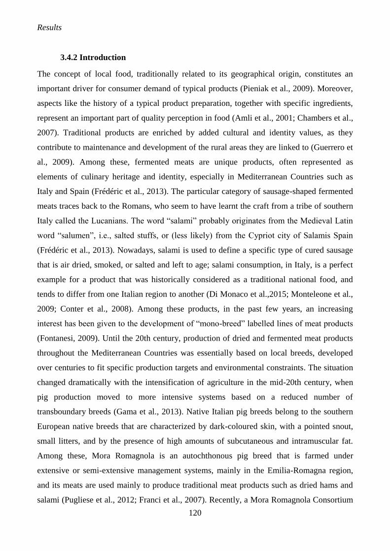
Results
120
3.4.2 Introduction
The concept of local food, traditionally related to its geographical origin, constitutes an
important driver for consumer demand of typical products (Pieniak et al., 2009). Moreover,
aspects like the history of a typical product preparation, together with specific ingredients,
represent an important part of quality perception in food (Amli et al., 2001; Chambers et al.,
2007). Traditional products are enriched by added cultural and identity values, as they
contribute to maintenance and development of the rural areas they are linked to (Guerrero et
al., 2009). Among these, fermented meats are unique products, often represented as
elements of culinary heritage and identity, especially in Mediterranean Countries such as
Italy and Spain (Frédéric et al., 2013). The particular category of sausage-shaped fermented
meats traces back to the Romans, who seem to have learnt the craft from a tribe of southern
Italy called the Lucanians. The word “salami” probably originates from the Medieval Latin
word “salumen”, i.e., salted stuffs, or (less likely) from the Cypriot city of Salamis Spain
(Frédéric et al., 2013). Nowadays, salami is used to define a specific type of cured sausage
that is air dried, smoked, or salted and left to age; salami consumption, in Italy, is a perfect
example for a product that was historically considered as a traditional national food, and
tends to differ from one Italian region to another (Di Monaco et al.,2015; Monteleone et al.,
2009; Conter et al., 2008). Among these products, in the past few years, an increasing
interest has been given to the development of “mono-breed” labelled lines of meat products
(Fontanesi, 2009). Until the 20th century, production of dried and fermented meat products
throughout the Mediterranean Countries was essentially based on local breeds, developed
over centuries to fit specific production targets and environmental constraints. The situation
changed dramatically with the intensification of agriculture in the mid-20th century, when
pig production moved to more intensive systems based on a reduced number of
transboundary breeds (Gama et al., 2013). Native Italian pig breeds belong to the southern
European native breeds that are characterized by dark-coloured skin, with a pointed snout,
small litters, and by the presence of high amounts of subcutaneous and intramuscular fat.
Among these, Mora Romagnola is an autochthonous pig breed that is farmed under
extensive or semi-extensive management systems, mainly in the Emilia-Romagna region,
and its meats are used mainly to produce traditional meat products such as dried hams and
salami (Pugliese et al., 2012; Franci et al., 2007). Recently, a Mora Romagnola Consortium
Results
121
has been founded to promote and increase the visibility of Mora Romagnola products and to
protect them from potential fraud. However, there is a lack of detailed information
concerning the quality properties and the sensory traits of traditional products made with
Mora Romagnola. The inimitable sensory characteristics of dry-fermented salami are
ascribed to a number of biochemical and physicochemical transformations occurring in the
sausage batter during fermentation and maturation. A distinctive gel-like texture is created
due to the bacterial acidification process, while specific color development results from
interactions between the myoglobin of the meat and nitrogen monoxide, originating from
the nitrate and/or nitrite in the curing salt (Gama et al., 2013). Finally, the complex flavor of
fermented sausages is due to oxidative transformations, mostly of unsaturated fatty acids,
and complex interactions between the sausage batter, meat enzymes, and microorganisms.
As a result, flavor development does not depend only on the raw materials and processing
conditions, but also on how these factors affect the composition, community dynamics, and
metabolism of the sausage microbiota (Gama et al., 2013). As a consequence,
characterization of the sensory profile of salami is very complex and requires the use of an
advanced and wide range of sensory and analytical techniques. Therefore, the aim of this
study was to highlight the relevance of the adoption of an integrated approach to describe
salami produced with the Mora Romagnola breed by comparing this typical product to
salami obtained using modern white-pig breeds available on the Italian market. For this
purpose, the product was characterized by an advanced analytical approach using sensory
descriptive analysis (DA) and instrumental techniques, such as image analysis by electronic
eye, solid-phase microextraction coupled with gas-chromatography mass-spectrometry
(SPME-GC-MS) forthe determination of the volatile profile, and a TA-HDi Heavy Duty
texture analyzer.
3.4.3 Materials and methods
3.4.3a Samples
The 13 samples selected for this study are listed in Table 1. In particular, 5 samples were
produced using meat from the Mora Romagnola breed, while the other 8 were manufactured
by meat from conventional pig breeds. The conventional samples “Contadino” (CON),
“Felino” (FEL), and “Milano” (MIL) were selected as they are market leaders in Italy
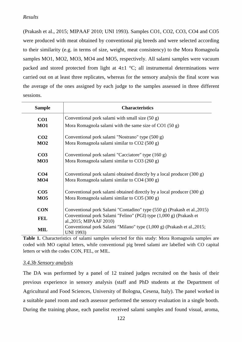
Results
122
(Prakash et al., 2015; MIPAAF 2010; UNI 1993). Samples CO1, CO2, CO3, CO4 and CO5
were produced with meat obtained by conventional pig breeds and were selected according
to their similarity (e.g. in terms of size, weight, meat consistency) to the Mora Romagnola
samples MO1, MO2, MO3, MO4 and MO5, respectively. All salami samples were vacuum
packed and stored protected from light at 4±1 °C; all instrumental determinations were
carried out on at least three replicates, whereas for the sensory analysis the final score was
the average of the ones assigned by each judge to the samples assessed in three different
sessions.
Sample Characteristics
CO1
Conventional pork salami with small size (50 g)
MO1 Mora Romagnola salami with the same size of CO1 (50 g)
CO2 Conventional pork salami "Nostrano" type (500 g)
MO2 Mora Romagnola salami similar to CO2 (500 g)
CO3 Conventional pork salami "Cacciatore" type (160 g)
MO3 Mora Romagnola salami similar to CO3 (260 g)
CO4 Conventional pork salami obtained directly by a local producer (300 g)
MO4 Mora Romagnola salami similar to CO4 (300 g)
CO5 Conventional pork salami obtained directly by a local producer (300 g)
MO5 Mora Romagnola salami similar to CO5 (300 g)
CON Conventional pork Salami "Contadino" type (550 g) (Prakash et al.,2015)
FEL Conventional pork Salami "Felino" (PGI) type (1,000 g) (Prakash et
al.,2015; MIPAAF 2010)
MIL Conventional pork Salami "Milano" type (1,000 g) (Prakash et al.,2015;
UNI 1993)
Table 1. Characteristics of salami samples selected for this study: Mora Romagnola samples are
coded with MO capital letters, while conventional pig breed salami are labelled with CO capital
letters or with the codes CON, FEL, or MIL.
3.4.3b Sensory analysis
The DA was performed by a panel of 12 trained judges recruited on the basis of their
previous experience in sensory analysis (staff and PhD students at the Department of
Agricultural and Food Sciences, University of Bologna, Cesena, Italy). The panel worked in
a suitable panel room and each assessor performed the sensory evaluation in a single booth.
During the training phase, each panelist received salami samples and found visual, aroma,
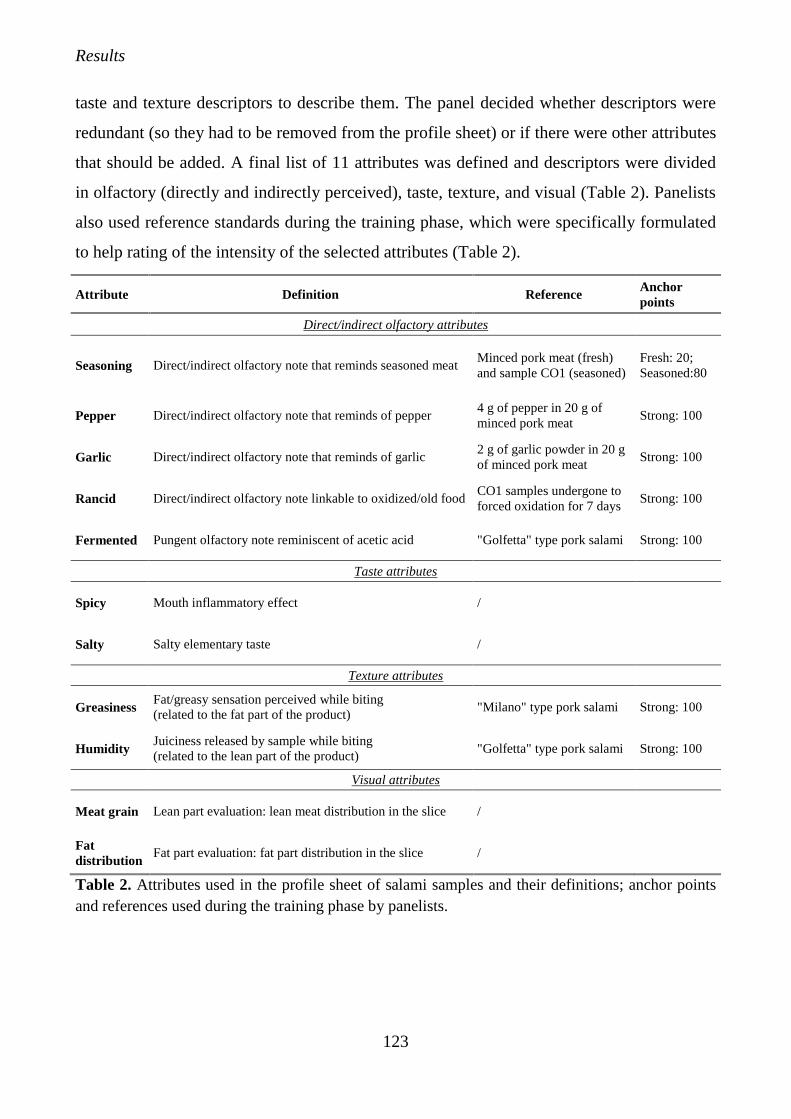
Results
123
taste and texture descriptors to describe them. The panel decided whether descriptors were
redundant (so they had to be removed from the profile sheet) or if there were other attributes
that should be added. A final list of 11 attributes was defined and descriptors were divided
in olfactory (directly and indirectly perceived), taste, texture, and visual (Table 2). Panelists
also used reference standards during the training phase, which were specifically formulated
to help rating of the intensity of the selected attributes (Table 2).
Attribute Definition Reference Anchor
points
Direct/indirect olfactory attributes
Seasoning Direct/indirect olfactory note that reminds seasoned meat Minced pork meat (fresh)
and sample CO1 (seasoned)
Fresh: 20;
Seasoned:80
Pepper Direct/indirect olfactory note that reminds of pepper 4 g of pepper in 20 g of
minced pork meat Strong: 100
Garlic Direct/indirect olfactory note that reminds of garlic 2 g of garlic powder in 20 g
of minced pork meat Strong: 100
Rancid Direct/indirect olfactory note linkable to oxidized/old food CO1 samples undergone to
forced oxidation for 7 days Strong: 100
Fermented Pungent olfactory note reminiscent of acetic acid "Golfetta" type pork salami Strong: 100
Taste attributes
Spicy Mouth inflammatory effect /
Salty Salty elementary taste /
Texture attributes
Greasiness Fat/greasy sensation perceived while biting
(related to the fat part of the product) "Milano" type pork salami Strong: 100
Humidity Juiciness released by sample while biting
(related to the lean part of the product) "Golfetta" type pork salami Strong: 100
Visual attributes
Meat grain Lean part evaluation: lean meat distribution in the slice /
Fat
distribution Fat part evaluation: fat part distribution in the slice /
Table 2. Attributes used in the profile sheet of salami samples and their definitions; anchor points
and references used during the training phase by panelists.
Results
124
The attributes were presented to each panelist and specific training sessions on their use
were carried out. Visual analysis of samples was performed at the end of each session in
white light conditions, while the rest of sensory evaluation was conducted using a red light,
in order to prevent the judge’s recognition of samples. The evaluation of red intensity of
salami was too difficult, as declared by the judges; during training, they were not able to
rate different intensities of red among the samples, and this attribute was thus removed from
the final profile sheet. The panelists rated samples by indicating the intensities of attributes
on an unstructured 100 mm scale with defined anchor points from 0 (not perceivable) on the
left side, to 100 (perceivable at maximum level) on the right. Samples were presented to
panelists in a randomized order; each session was performed on four different samples, all
presented as whole slices cut with a fixed thickness of 3 mm. Salami were coded with
alphanumerical codes and presented in white plastic dishes. Fresh water and breadsticks
were provided to panelists between sample evaluation to clean their mouth. The software
FIZZ (Biosystèmes, Dijon, France) was used to create the profile sheet adopted during
sensory evaluation and for related data collection. Samples were analyzed in triplicate.
3.4.3c Volatile compounds analysis
An aliquot of 1 g of each sample, previously homogenized with a mixer, was weighed in a
20 mL amber glass vial. Each vial was closed with a silicone septum and conditioned at
40°C for 2 min. After this, a divinylbenzene/carboxen/polydimethylsiloxane
(DVB/CAR/PDMS) fiber (50/30 µm, 2 cm long from Supelco Ltd., Bellefonte, PA) was
exposed to the sample headspace for 30 min and immediately desorbed for 5 min at 240°C
in the GC injector, with a split ratio of 1:10. Analytes were separated on a ZB-WAX column
30 m × 0.25 mm ID, 1.00 µm film thickness (Phenomenex, Torrance, CA, USA). Column
temperature was held at 40°C for 10 min and increased to 200°C at 3°C min-1. After 3 min,
the temperature increased to 240°C at 10°C min-1 and remained stable for 5 min. Helium
was used as a carrier gas at a flow of 1 ml min-1. Volatile compounds were analyzed by
quadrupolar mass-selective spectrometry (in the 30–250 amu mass range), using a GCMS-
QP2010 gas chromatograph (Shimadzu Co., Kyoto, Japan) coupled with an autosampler
AOC-5000 Plus (Shimadzu Co., Kyoto, Japan). Peak identification was based on
comparison of mass spectrum data with spectra present in the National Institute of
Standards and Technology (NIST) library (2008 version) and only identification matching
Results
125
more than 90% were taking into account. Since it was not possible to use an internal
standard (due to the difficulty to homogenously solubilize a standard molecule in a solid
sample), a percentage normalization was applied: the presence of each compound was
expressed as percentage with respect to the entire volatile fraction. Three replicates for each
sample were performed.
3.4.3d Image analysis
The instrumental measurement of appearance was carried out by an “electronic eye” (Visual
Analyzer VA400 IRIS, Alpha MOS, France), a high-resolution CCD (charge-coupled
device) camera (resolution 2592 × 1944 p) combined with powerful data processing
software. This instrument was equipped with an adjustable photo-camera (16 million colors)
in a dedicated measurement small room with standardized, controlled and reproducible
lighting conditions. The camera imaging was software-monitored, and equipped with
several lenses of different focal length for accurately assessing from very small to large
products. The instrument is furnished with top and bottom lighting (2*2 fluorescent tubes)
6700°K colour temperature and IRC = 98 (near D65: daylight during a cloudy day at 12
AM) and has to be turned on 15 minutes at least before acquisition for lighting stabilization.
Samples were placed on a removable white tray, diffusing a uniform light inside the
device’s 600 × 600 × 750-mm closable light chamber and the CCD camera takes a picture.
The instrument is able to undergo automatic calibration with a certified colour checker, and
image analysis (RGB scale or CIE L*a*b*) and statistical analysis were carried out using
the advanced software available in the instrument (Alphasoft, version 14.0). The data
processing software extracts color parameters from the picture and it is also possible to
correlate these data with ones from sensory panels, if provided.
3.4.3e Textural properties
Warner Bratzler shear test was performed by shearing a 4 × 1 × 1cm parallelepiped samples
by a TA-HDi Heavy Duty texture analyzer (Stable Micro Systems Ltd., Godalming, Surrey,
UK) (5 replications/sample) (Del Nobile et al., 2009). The instrument, equipped with a 25kg
loading cell and a Warner-Bratzler triangular shear blade, was set to shear the sample at a
Results
126
cross head speed of 2 mm/sec. Shear force was defined as the maximum force (expressed as
kilograms) required to shear the sample.
Texture profile analysis (TPA) was performed on a cylindrical-shaped meat sample (3 cm
diameter × 0.8 cm height) that was double compressed to 60% of its initial height (5
replications/sample). The test was run by using a TA-HDi Heavy Duty texture analyzer
(Stable Micro Systems Ltd., Godalming, Surrey, UK) equipped with a 25 kg loading cell
and a 5 cm-diameter cylindrical aluminum probe. Next, the TPA parameters of Hardness,
Cohesiveness, Springiness, Gumminess and Chewiness were obtained by elaborating the
double compression diagram (force/deformation) of each sample (De Campos et al., 2008).
Tensile test was performed on a hexagonal sample (25 mm-long × 2 mm-thick; 5
replications/sample) according to the procedure described by Herrero et al. (Herrero et al.,
2008). Briefly, tensile properties were evaluated by using a TA-HDi Heavy Duty texture
analyzer (Stable Micro Systems Ltd., Godalming, Surrey, UK) equipped with a 5 kg loading
cell and two tensile grips (one fixed to the base of the texture analyser and the second
attached to the loading cell). After applying a grip separation of 25 mm at a cross-head
speed of 1 mm/s, rupture force, defined as the maximum peak force required for breaking
the sample (kg), and breaking strength, defined as the ratio between rupture force and cross-
sectional area of the sample (kg/cm2), were calculated.
3.4.3f Statistical analysis
The software XLSTAT 7.5.2 version (Addinsoft, Belmont, MA) was used to elaborate data
using the analysis of variance (ANOVA, with Fishers’ least square difference post-hoc test)
and to elaborate data from chemical (volatile compounds), sensory, and textural property
analyses through multifactorial analysis (MFA). The software Alphasoft version 14.0
(Alpha MOS, France) was used to explore data from image analysis with Principal
Component Analysis (PCA).
3.4.4 Results and discussion
3.4.4a Sensory analysis
The reliability of the panel's performance and training efficiency was checked to ensure
reproducibility and repeatability were good (data not shown). Additionally, panel analysis
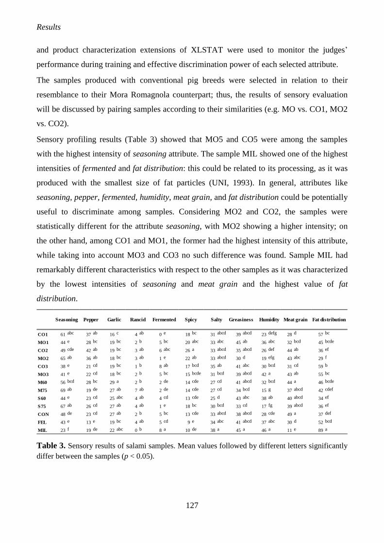
Results
127
and product characterization extensions of XLSTAT were used to monitor the judges’
performance during training and effective discrimination power of each selected attribute.
The samples produced with conventional pig breeds were selected in relation to their
resemblance to their Mora Romagnola counterpart; thus, the results of sensory evaluation
will be discussed by pairing samples according to their similarities (e.g. MO vs. CO1, MO2
vs. CO2).
Sensory profiling results (Table 3) showed that MO5 and CO5 were among the samples
with the highest intensity of seasoning attribute. The sample MIL showed one of the highest
intensities of fermented and fat distribution: this could be related to its processing, as it was
produced with the smallest size of fat particles (UNI, 1993). In general, attributes like
seasoning, pepper, fermented, humidity, meat grain, and fat distribution could be potentially
useful to discriminate among samples. Considering MO2 and CO2, the samples were
statistically different for the attribute seasoning, with MO2 showing a higher intensity; on
the other hand, among CO1 and MO1, the former had the highest intensity of this attribute,
while taking into account MO3 and CO3 no such difference was found. Sample MIL had
remarkably different characteristics with respect to the other samples as it was characterized
by the lowest intensities of seasoning and meat grain and the highest value of fat
distribution.
CO1 61 abc 37 ab 16 c 4 ab 0 e 18 bc 31 abcd 39 abcd 23 defg 28 d 57 bc
MO1 44 e 28 bc 19 bc 2 b 5 bc 20 abc 33 abc 45 ab 36 abc 32 bcd 45 bcde
CO2 49 cde 42 ab 19 bc 3 ab 6 abc 26 a 33 abcd 35 abcd 26 def 44 ab 36 ef
MO2 65 ab 36 ab 18 bc 3 ab 1 e 22 ab 33 abcd 30 d 19 efg 43 abc 29 f
CO3 38 e 21 cd 19 bc 1 b 8 ab 17 bcd 35 ab 41 abc 30 bcd 31 cd 59 b
MO3 41 e 22 cd 18 bc 2 b 5 bc 15 bcde 31 bcd 39 abcd 42 a 43 ab 55 bc
M60 56 bcd 28 bc 29 a 2 b 2 de 14 cde 27 cd 41 abcd 32 bcd 44 a 46 bcde
M75 69 ab 19 de 27 ab 7 ab 2 de 14 cde 27 cd 34 bcd 15 g 37 abcd 42 cdef
S60 44 e 23 cd 25 abc 4 ab 4 cd 13 cde 25 d 43 abc 38 ab 40 abcd 34 ef
S75 67 ab 26 cd 27 ab 4 ab 1 e 18 bc 30 bcd 33 cd 17 fg 39 abcd 36 ef
CON 48 de 23 cd 27 ab 2 b 5 bc 13 cde 33 abcd 38 abcd 28 cde 49 a 37 def
FEL 43 e 13 e 19 bc 4 ab 5 cd 9 e 34 abc 41 abcd 37 abc 30 d 52 bcd
MIL 23 f 19 de 22 abc 0 b 8 a 10 de 38 a 45 a 46 a 11 e 89 a
Seasoning Fat distributionMeat grainHumidityGreasinessSaltySpicyFermentedRancidGarlicPepper
Table 3. Sensory results of salami samples. Mean values followed by different letters significantly
differ between the samples (p < 0.05).
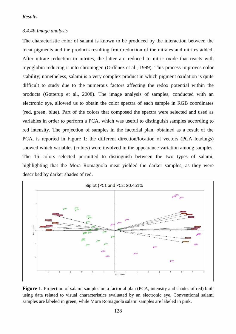
Results
128
3.4.4b Image analysis
The characteristic color of salami is known to be produced by the interaction between the
meat pigments and the products resulting from reduction of the nitrates and nitrites added.
After nitrate reduction to nitrites, the latter are reduced to nitric oxide that reacts with
myoglobin reducing it into chromogen (Ordònez et al., 1999). This process improves color
stability; nonetheless, salami is a very complex product in which pigment oxidation is quite
difficult to study due to the numerous factors affecting the redox potential within the
products (Gøtterup et al., 2008). The image analysis of samples, conducted with an
electronic eye, allowed us to obtain the color spectra of each sample in RGB coordinates
(red, green, blue). Part of the colors that composed the spectra were selected and used as
variables in order to perform a PCA, which was useful to distinguish samples according to
red intensity. The projection of samples in the factorial plan, obtained as a result of the
PCA, is reported in Figure 1: the different direction/location of vectors (PCA loadings)
showed which variables (colors) were involved in the appearance variation among samples.
The 16 colors selected permitted to distinguish between the two types of salami,
highlighting that the Mora Romagnola meat yielded the darker samples, as they were
described by darker shades of red.
Figure 1. Projection of salami samples on a factorial plan (PCA, intensity and shades of red) built
using data related to visual characteristics evaluated by an electronic eye. Conventional salami
samples are labeled in green, while Mora Romagnola salami samples are labeled in pink.
Results
129
In particular, variables like “colors-2424” and “colors-2440”, which describes the strongest
red intensities, mainly described several Mora Romagnola samples. On the other hand,
variables like “colors-2951” and “colors-2678” mainly characterized samples from
conventional pig breeds.
This is an important result, as the judges declared that they were not able to evaluate the
differences in red intensities among samples. Thus, the use of an electronic eye could
support visual evaluation of red intensity in salami and could be useful for the
characterization of salami produced with meat from Mora Romagnola. Moreover, this result
could be used to define a specific range of color taints associated with Mora Romagnola
salami. Starting from this, a non-targeted colorimetric method could be established to
evaluate the conformity of different Mora Romagnola salami to their typical color.
3.4.4c Volatile compounds analysis
It is well known that during the processing of dry-cured meat products, many enzymatic and
non-enzymatic reactions occur such as protein degradation, lipid degradation and oxidation,
Maillard reactions, and Strecker degradation. These changes give rise to the formation of
volatile compounds such as aldehydes, carboxylic acids, alcohols, ketones, esters, terpenes
as well as sulfur, nitrogen, and other compounds (Jerkovic et al., 2010). In this
investigation, a total of 33 volatile compounds were tentatively identified in the sample
headspace; compounds are listed in Table 4 according to the chemical classes they belong
to. Low percentages of ketones were detected in all samples, with the exception of 2-
butanone that was present in a high amount in sample MO3 (12.76%): this molecule is
already known as one of the contributors for an “apricot” note in sausages (Olivares et al.,
2009). Considering alcohols, the compounds with highest amounts were ethanol and 2-
buthanol. In particular, ethanol was detected in all samples produced with Mora Romagnola,
with higher percentages compared to conventional samples CO1, CO2, and CO3. This
compound can derive from the reduction of aldehydes formed by lipid metabolism (Marco
et al., 2008) or from microbial fermentation (Procida et al., 1999); other alcohols such as
pentanol, hexanol, and octen-3-ol are also produced in the same way; the latter is considered
to be responsible for the mushroom-like odor (Montel et al., 1998) and is produced during
Results
130
degradation of lipid hydroperoxides (Frankel, 2014). The seasoning process of salami is
known to have an important role in the formation of aldehydes; the main precursors of these
compounds in meat products are unsaturated fatty acids (Moretti et al.,2004). Among
aldehydes, hexanal was the most represented; this molecule showed the highest percentage
compared to other volatile compounds detected in salami. Hexanal is already known to
impart green, grassy, or floral notes (Meynier et al., 1999; Stanhke, 1995); the highest
percentages of hexanal were recorded for samples FEL (72.58%), CON (46.86%), CO5
(44.78%), and MIL (31.56%). The second most abundant aldehyde is represented by
phenylacetaldehyde, with the highest percentage (38.07 %) in MO4; all the other samples
showed lower abundances of this molecule, an aroma-active compound formed from
phenylalanine through the Strecker degradation pathway (Hoffman et al., 2000). Allyl
methyl sulfide is a volatile sulfur-containing compound, responsible for sensory garlic notes
and naturally present in many plants from Allium, such as garlic, onion and leek (Lanzotti,
2006); this compound was detected in samples CO3, MO3, CO4, CO5, MO4, and MO5
(few amounts in MO1 and MO2). In accordance with previous studies (Moretti et al., 2004),
the chemical class of terpenes was the most represented, whose presence is probably due to
addition of spices during salami preparation. In fact, α-pinene, identified in all samples
except for FEL, is a terpene already found in coniferous and rosemary essential oil
(Simonsen et al., 1957). The same origin is attributed to β-pinene, which showed the highest
percentage in CO1 (26.58%). The isomers of α-phellandrene and β-phellandrene are specific
to certain plants: the first is typical of Eucalyptus phellandra, while the latter has been
frequently found in fennel essential oil (Tholl et al., 2006). 3-carene, a molecule linked to
pepper scents, was mainly found in samples CO4, MO4, CO5, and MO5, produced with the
same recipe, while limonene was the most represented terpene and can be associated with
pine/peppery/lemon sensory notes (El Zaeddi et al., 2017). Caryophyllene reminds of
sensory notes of clover/turpentine, which could match the characteristic ‘green flavor”
(Burdock, 2016). As reported in previous studies, the presence of many terpenes may be
associated with the use of spices, mainly pepper and garlic (Moretti et al., 2004; Meynier et
al., 1999). It is interesting to highlight how sample FEL did not show the presence of
terpenes; thus, it could be hypothesized that spices were not added to the meat during
preparation. Finally, several acids were identified: butanoic acid is a carboxylic acid coming
Results
131
from hydrolysis of glycerides and could be responsible of rancid perception in food
(Stahnke et al., 1995): this molecule was detected only in samples MO1, CO3, and MIL,
while the most abundant acid was acetic acid, which showed the highest percentage in
sample MIL (10.79%); the same behavior was also recorded for 3-methylbutanoic acid. The
findings of this study on volatile compounds highlighted that, although several volatile
compounds were significantly different among samples, there was no trend related to the
different type (Mora Romagnola vs. conventional) of meat used. Conversely, it seemed that
samples available on the market showed remarkably differences in terms of aromatic
profile: this result could be associated with the product preparation and use of different
spices. In this context, market leader products were characterized by a reduced number of
volatiles: no terpenes were detected in samples FEL; in addition, ethanol was not detected in
CON, FEL, or MIL. On the other hand, substantial variability was reported among the Mora
Romagnola samples, which may be related to the different dimensions and weights, or to the
curing period. This is not an unexpected result, since salami produced with this local breed
are traditional products, whose recipes (specific ingredients) and handcraft preparation are
characterized by a certain variability, linkable to the concept of local food (Amli et al.,
2011; Chambers et al., 2007).
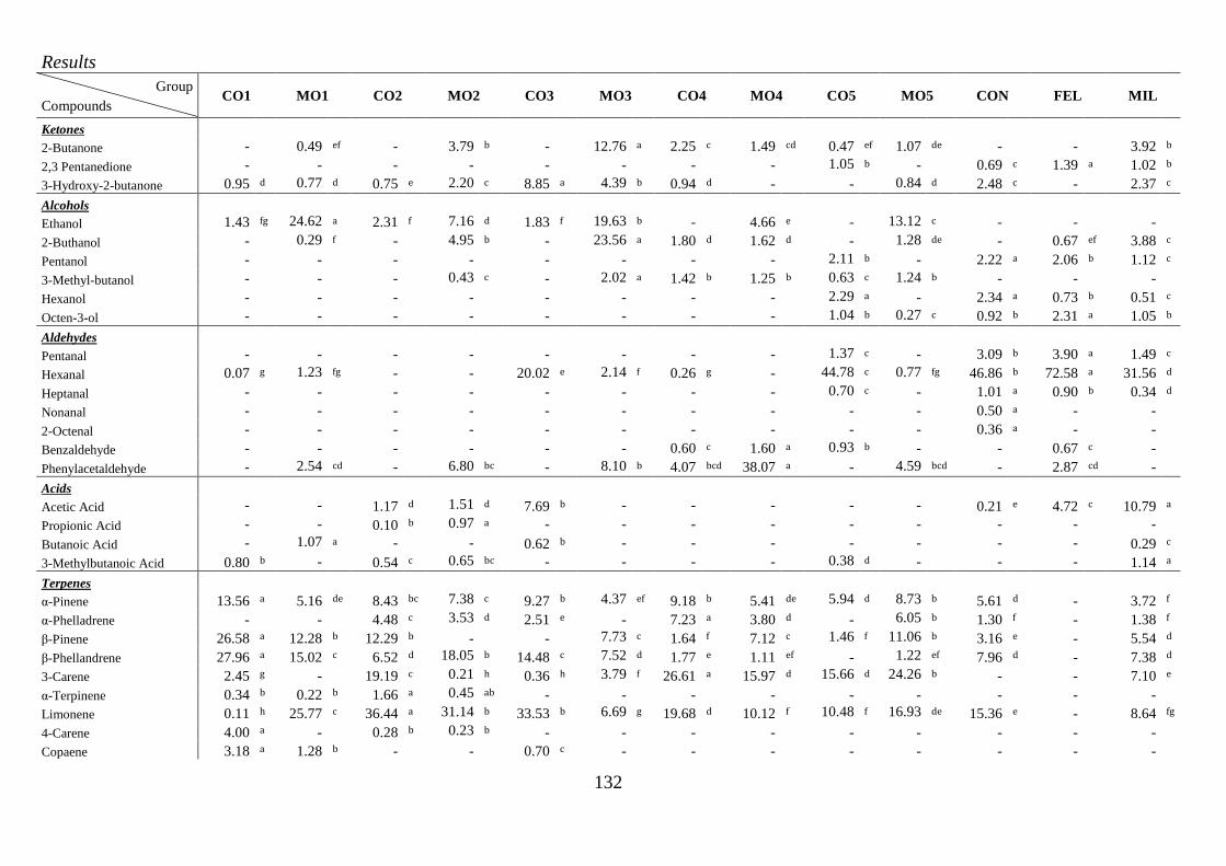
Results
132
Group
Compounds CO1 MO1 CO2 MO2 CO3 MO3 CO4 MO4 CO5 MO5 CON FEL MIL
Ketones 2-Butanone - 0.49 ef - 3.79 b - 12.76 a 2.25 c 1.49 cd 0.47 ef 1.07 de - - 3.92 b 2,3 Pentanedione - - - - - - - - 1.05 b - 0.69 c 1.39 a 1.02 b 3-Hydroxy-2-butanone 0.95 d 0.77 d 0.75 e 2.20 c 8.85 a 4.39 b 0.94 d - - 0.84 d 2.48 c - 2.37 c
Alcohols Ethanol 1.43 fg 24.62 a 2.31 f 7.16 d 1.83 f 19.63 b - 4.66 e - 13.12 c - - - 2-Buthanol - 0.29 f - 4.95 b - 23.56 a 1.80 d 1.62 d - 1.28 de - 0.67 ef 3.88 c Pentanol - - - - - - - - 2.11 b - 2.22 a 2.06 b 1.12 c 3-Methyl-butanol - - - 0.43 c - 2.02 a 1.42 b 1.25 b 0.63 c 1.24 b - - - Hexanol - - - - - - - - 2.29 a - 2.34 a 0.73 b 0.51 c Octen-3-ol - - - - - - - - 1.04 b 0.27 c 0.92 b 2.31 a 1.05 b Aldehydes Pentanal - - - - - - - - 1.37 c - 3.09 b 3.90 a 1.49 c Hexanal 0.07 g 1.23 fg - - 20.02 e 2.14 f 0.26 g - 44.78 c 0.77 fg 46.86 b 72.58 a 31.56 d Heptanal - - - - - - - - 0.70 c - 1.01 a 0.90 b 0.34 d Nonanal - - - - - - - - - - 0.50 a - - 2-Octenal - - - - - - - - - - 0.36 a - - Benzaldehyde - - - - - - 0.60 c 1.60 a 0.93 b - - 0.67 c - Phenylacetaldehyde - 2.54 cd - 6.80 bc - 8.10 b 4.07 bcd 38.07 a - 4.59 bcd - 2.87 cd -
Acids Acetic Acid - - 1.17 d 1.51 d 7.69 b - - - - - 0.21 e 4.72 c 10.79 a Propionic Acid - - 0.10 b 0.97 a - - - - - - - - - Butanoic Acid - 1.07 a - - 0.62 b - - - - - - - 0.29 c 3-Methylbutanoic Acid 0.80 b - 0.54 c 0.65 bc - - - - 0.38 d - - - 1.14 a
Terpenes α-Pinene 13.56 a 5.16 de 8.43 bc 7.38 c 9.27 b 4.37 ef 9.18 b 5.41 de 5.94 d 8.73 b 5.61 d - 3.72 f α-Phelladrene - - 4.48 c 3.53 d 2.51 e - 7.23 a 3.80 d - 6.05 b 1.30 f - 1.38 f β-Pinene 26.58 a 12.28 b 12.29 b - - 7.73 c 1.64 f 7.12 c 1.46 f 11.06 b 3.16 e - 5.54 d β-Phellandrene 27.96 a 15.02 c 6.52 d 18.05 b 14.48 c 7.52 d 1.77 e 1.11 ef - 1.22 ef 7.96 d - 7.38 d 3-Carene 2.45 g - 19.19 c 0.21 h 0.36 h 3.79 f 26.61 a 15.97 d 15.66 d 24.26 b - - 7.10 e α-Terpinene 0.34 b 0.22 b 1.66 a 0.45 ab - - - - - - - - - Limonene 0.11 h 25.77 c 36.44 a 31.14 b 33.53 b 6.69 g 19.68 d 10.12 f 10.48 f 16.93 de 15.36 e - 8.64 fg 4-Carene 4.00 a - 0.28 b 0.23 b - - - - - - - - - Copaene 3.18 a 1.28 b - - 0.70 c - - - - - - - -
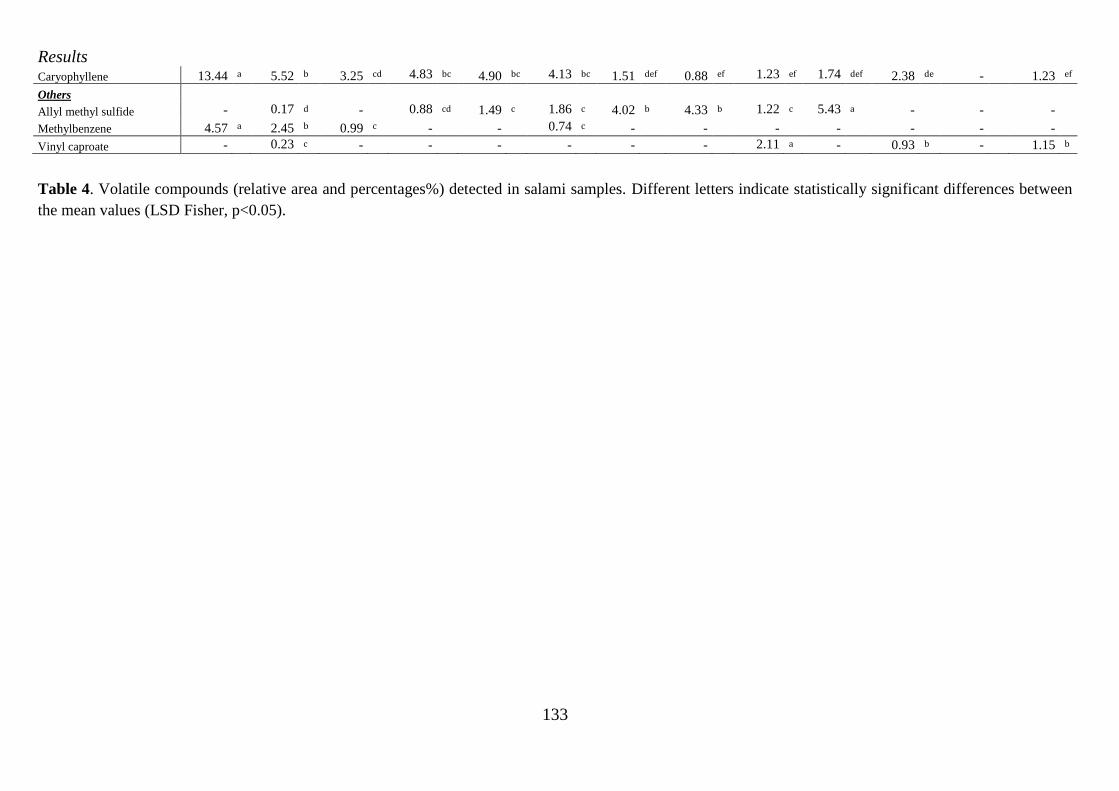
Results
133
Caryophyllene 13.44 a 5.52 b 3.25 cd 4.83 bc 4.90 bc 4.13 bc 1.51 def 0.88 ef 1.23 ef 1.74 def 2.38 de - 1.23 ef
Others Allyl methyl sulfide - 0.17 d - 0.88 cd 1.49 c 1.86 c 4.02 b 4.33 b 1.22 c 5.43 a - - - Methylbenzene 4.57 a 2.45 b 0.99 c - - 0.74 c - - - - - - -
Vinyl caproate - 0.23 c - - - - - - 2.11 a - 0.93 b - 1.15 b
Table 4. Volatile compounds (relative area and percentages%) detected in salami samples. Different letters indicate statistically significant differences between
the mean values (LSD Fisher, p<0.05).
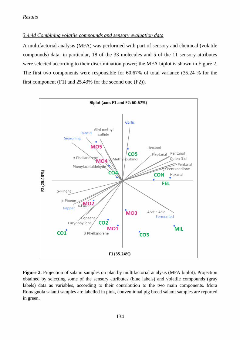
Results
134
3.4.4d Combining volatile compounds and sensory evaluation data
A multifactorial analysis (MFA) was performed with part of sensory and chemical (volatile
compounds) data: in particular, 18 of the 33 molecules and 5 of the 11 sensory attributes
were selected according to their discrimination power; the MFA biplot is shown in Figure 2.
The first two components were responsible for 60.67% of total variance (35.24 % for the
first component (F1) and 25.43% for the second one (F2)).
Figure 2. Projection of salami samples on plan by multifactorial analysis (MFA biplot). Projection
obtained by selecting some of the sensory attributes (blue labels) and volatile compounds (gray
labels) data as variables, according to their contribution to the two main components. Mora
Romagnola salami samples are labelled in pink, conventional pig breed salami samples are reported
in green.
Results
135
The outcomes highlighted that samples MO4, MO5, CO4 and CO5 were similar and close
to the attributes seasoning, rancid, and garlic and to volatile compounds related to oxidation
(phenylacetaldehyde) and garlic (allyl methyl sulfide). Moreover, the attributes seasoning
and rancid were positively correlated (r = 0.75); thus, it could be hypothesized that an
increased intensity of seasoning attribute could be linked to a stronger perception of rancid
descriptor. Samples MO1, MO2, CO1, and CO2 were characterized by the presence of
many terpenes and by the sensory attribute of pepper. This latter descriptor was positively
correlated with the presence of volatile compounds such as caryophyllene, β-phellandrene,
and α-pinene. This finding is in agreement with previous studies (Plessi et al., 2002;
Meynier et al., 1999), where the aforementioned terpenes were reposted to be responsible
for the perception of spicy notes, in particular with pepper. Samples MO3 and CO3 were
characterized by the presence of acetic acid and the sensory perception of fermented, which
were positively correlated (r = 0.69). This result is in accordance with Stankhe et al. (1995),
since the acid perception in salami was associated with sensory notes of fermented or
pungent.
3.4.4e Textural properties
The findings for textural properties assessed by Warner-Bratzler shear blade, TPA, and
tensile test are reported in Table 5. If the entire set of samples is considered, as expected it
can be clearly observed that, exhibiting the lowest values for all the parameters, MIL
displayed remarkably different textural properties than the other samples. On the other hand,
both FEL and CON exhibited a texture profile comparable to those of the 10 experimental
groups. Within this context, since the conventional samples were selected according to the
similarity with their Mora Romagnola counterpart, the results for textural properties will be
discussed considering the samples as pairs. No significant differences were found in the
texture profile of CO1 and MO1, which exhibited analogous values for almost all the
parameters considered herein. Similarly, only negligible dissimilarities (not displaying any
clear trends) were observed by comparing the textural properties of CO3 vs. MO3 and CO4
vs. MO4 samples. On the other hand, the main differences in the textural properties of
conventional vs. Mora Romagnola samples were observed by comparing CO2 vs. MO2 and
CO5 vs. MO5.
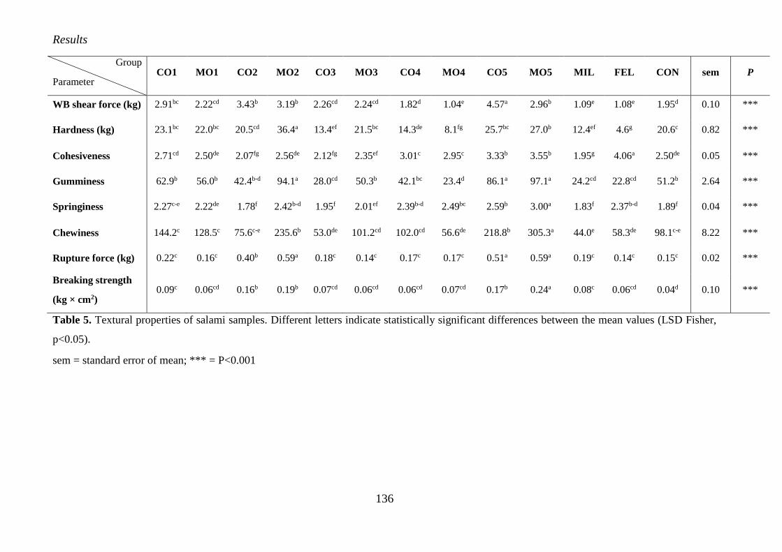
Results
136
Table 5. Textural properties of salami samples. Different letters indicate statistically significant differences between the mean values (LSD Fisher,
p<0.05).
sem = standard error of mean; *** = P<0.001
Group
Parameter CO1 MO1 CO2 MO2 CO3 MO3 CO4 MO4 CO5 MO5 MIL FEL CON sem P
WB shear force (kg) 2.91bc 2.22cd 3.43b 3.19b 2.26cd 2.24cd 1.82d 1.04e 4.57a 2.96b 1.09e 1.08e 1.95d 0.10 ***
Hardness (kg) 23.1bc 22.0bc 20.5cd 36.4a 13.4ef 21.5bc 14.3de 8.1fg 25.7bc 27.0b 12.4ef 4.6g 20.6c 0.82 ***
Cohesiveness 2.71cd 2.50de 2.07fg 2.56de 2.12fg 2.35ef 3.01c 2.95c 3.33b 3.55b 1.95g 4.06a 2.50de 0.05 ***
Gumminess 62.9b 56.0b 42.4b-d 94.1a 28.0cd 50.3b 42.1bc 23.4d 86.1a 97.1a 24.2cd 22.8cd 51.2b 2.64 ***
Springiness 2.27c-e 2.22de 1.78f 2.42b-d 1.95f 2.01ef 2.39b-d 2.49bc 2.59b 3.00a 1.83f 2.37b-d 1.89f 0.04 ***
Chewiness 144.2c 128.5c 75.6c-e 235.6b 53.0de 101.2cd 102.0cd 56.6de 218.8b 305.3a 44.0e 58.3de 98.1c-e 8.22 ***
Rupture force (kg) 0.22c 0.16c 0.40b 0.59a 0.18c 0.14c 0.17c 0.17c 0.51a 0.59a 0.19c 0.14c 0.15c 0.02 ***
Breaking strength
(kg × cm2) 0.09c 0.06cd 0.16b 0.19b 0.07cd 0.06cd 0.06cd 0.07cd 0.17b 0.24a 0.08c 0.06cd 0.04d 0.10 ***
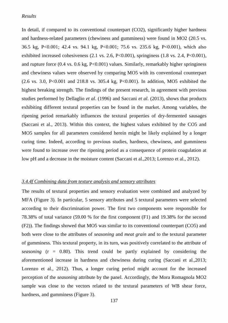
Results
137
In detail, if compared to its conventional counterpart (CO2), significantly higher hardness
and hardness-related parameters (chewiness and gumminess) were found in MO2 (20.5 vs.
36.5 kg, P<0.001; 42.4 vs. 94.1 kg, P<0.001; 75.6 vs. 235.6 kg, P<0.001), which also
exhibited increased cohesiveness (2.1 vs. 2.6, P<0.001), springiness (1.8 vs. 2.4, P<0.001),
and rupture force (0.4 vs. 0.6 kg, P<0.001) values. Similarly, remarkably higher springiness
and chewiness values were observed by comparing MO5 with its conventional counterpart
(2.6 vs. 3.0, P<0.001 and 218.8 vs. 305.4 kg, P<0.001). In addition, MO5 exhibited the
highest breaking strength. The findings of the present research, in agreement with previous
studies performed by Dellaglio et al. (1996) and Saccani et al. (2013), shows that products
exhibiting different textural properties can be found in the market. Among variables, the
ripening period remarkably influences the textural properties of dry-fermented sausages
(Saccani et al., 2013). Within this context, the highest values exhibited by the CO5 and
MO5 samples for all parameters considered herein might be likely explained by a longer
curing time. Indeed, according to previous studies, hardness, chewiness, and gumminess
were found to increase over the ripening period as a consequence of protein coagulation at
low pH and a decrease in the moisture content (Saccani et al.,2013; Lorenzo et al., 2012).
3.4.4f Combining data from texture analysis and sensory attributes
The results of textural properties and sensory evaluation were combined and analyzed by
MFA (Figure 3). In particular, 5 sensory attributes and 5 textural parameters were selected
according to their discrimination power. The first two components were responsible for
78.38% of total variance (59.00 % for the first component (F1) and 19.38% for the second
(F2)). The findings showed that MO5 was similar to its conventional counterpart (CO5) and
both were close to the attributes of seasoning and meat grain and to the textural parameter
of gumminess. This textural property, in its turn, was positively correlated to the attribute of
seasoning (r = 0.80). This trend could be partly explained by considering the
aforementioned increase in hardness and chewiness during curing (Saccani et al.,2013;
Lorenzo et al., 2012). Thus, a longer curing period might account for the increased
perception of the seasoning attribute by the panel. Accordingly, the Mora Romagnola MO2
sample was close to the vectors related to the textural parameters of WB shear force,
hardness, and gumminess (Figure 3).
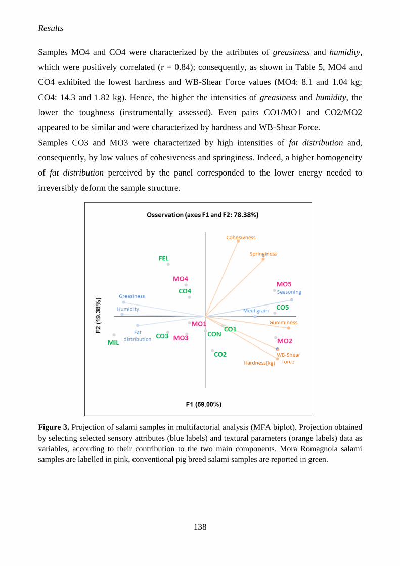
Results
138
Samples MO4 and CO4 were characterized by the attributes of greasiness and humidity,
which were positively correlated (r = 0.84); consequently, as shown in Table 5, MO4 and
CO4 exhibited the lowest hardness and WB-Shear Force values (MO4: 8.1 and 1.04 kg;
CO4: 14.3 and 1.82 kg). Hence, the higher the intensities of greasiness and humidity, the
lower the toughness (instrumentally assessed). Even pairs CO1/MO1 and CO2/MO2
appeared to be similar and were characterized by hardness and WB-Shear Force.
Samples CO3 and MO3 were characterized by high intensities of fat distribution and,
consequently, by low values of cohesiveness and springiness. Indeed, a higher homogeneity
of fat distribution perceived by the panel corresponded to the lower energy needed to
irreversibly deform the sample structure.
Figure 3. Projection of salami samples in multifactorial analysis (MFA biplot). Projection obtained
by selecting selected sensory attributes (blue labels) and textural parameters (orange labels) data as
variables, according to their contribution to the two main components. Mora Romagnola salami
samples are labelled in pink, conventional pig breed salami samples are reported in green.
Results
139
3.4.5 Conclusions
In conclusion, on the basis of an integrated approach, specific sensory and instrumental
parameters, useful to describe and discriminate Mora Romagnola salami, a typical Italian
product, were detected. In particular, the sensory evaluation, conducted by a panel of trained
judges, highlighted that the five Mora Romagnola salami here analysed were characterized
by the attributes: seasoning, pepper, fermented, humidity, meat grain and fat distribution.
Thirty-three volatile molecules, mainly belonging to the chemical classes of terpenes,
aldehydes, alcohols, ketones, and acids, were separated and detected by SPME-GC-MS. In
general, all the salami samples were characterized by the presence of aldehydes, as hexanal,
mainly produced during autoxidation, and by many terpenes. In particular, higher amounts
of terpenes as caryophyllene, β-phellandrene, and α-pinene, compounds due to the presence
of pepper, were detected in Mora Romagnola samples that were also characterized by a
higher intensity of the sensory attribute of pepper. Color differences among Mora
Romagnola and conventional salami resulted to be unperceivable by human eyes;
nevertheless, the electronic eye allowed to discriminate between samples produced with
different pig breeds. Specifically, Mora Romagnola samples showed darker shades of red
colour, if compared to their conventional counterpart. Salami produced with Mora
Romagnola and their conventional counterpart were not discriminated by the instrumental
texture analysis; on the other hand, the recipe, the dimension and the ripening are
responsible for the large variability of textural properties among samples. This result puts on
evidence that the traditional craftsmanship of this typical and local pig breed production
determines a certain variability among Mora Romagnola salami, linkable to the concept of
local food. The results of this rapid and integrated analytical approach can be useful to
provide quality elements and attributes to be included in a single document devoted to
describe and protect the peculiar characteristics of Mora Romagnola salami.
3.4.6 Aknowledgements
This work was supported by the Italian program FARB – Financing of Alma Mater
Studiorum – University of Bologna for basic research. Line of Action 2 – Project Meating
“sensory and fast instrumental analyses of meat and meat products: an integrated approach
for quality control and communication.”.
Results
140
3.4.7 References
Almli V.L., Verbeke W., Vanhonacker F., Næs T., Hersleth, M. 2011. General image and
attribute perceptions of traditional food in six European countries. Food Quality and
Preference, 22, 129-138.
Burdock G.A. 2016. Fenaroli's handbook of flavor ingredients. CRC press.
Chambers S., Lobb A., Butler L., Harvey K., Traill B. 2007. Local, national and imported
foods: a qualitative study. Appetite, 49, 208–213.
Conter M., Zanardi E., Ghidini S., Pennisi L., Vergara A., Campanini G., Ianieri A. 2008.
Consumers’ behaviour toward typical Italian dry sausages. Food Control, 19, 609-615.
De Campos R.M.L., Terra N.N., Campagnol P.C.B. 2008. Sensory aspects of cooked meats.
Pages 549–560. Handbook of Muscle Foods Analysis, eds. CRC Press, New York.
Del Nobile M.A., Conte A., Incoronato A.L., Panza O., Sevi A., Marino R. 2009. New
strategies for reducing the pork back-fat content in typical Italian salami. Meat Science, 81,
263-269.
Dellaglio, S., Casiraghi E., Pompei C. 1996. Chemical, physical and sensory attributes for the
characterization of an Italian dry-cured sausage. Meat Science, 42, 25-35.
Di Monaco R., Cavella S. 2015. Differences in liking of traditional salami: The effect of local
consumer familiarity and relation with the manufacturing process. British Food Journal,
117, 2039-2056.
El Zaeddi H., Martínez Tomé J., Calín Sánchez Á., Burló F., Carbonell Barrachina Á.A.
2017. Irrigation dose and plant density affect the volatile composition and sensory quality of
dill (Anethum graveolens L.). Journal of the Science of Food and Agriculture, 97, 427-433.
Fontanesi L., 2009. Genetic authentication and traceability of food products of animal origin:
new 398 developments and perspectives. Italian Journal of Animal Science, 8, 9-18.
Franci O., Pugliese C. 2007. Italian autochthonous pigs: progress report and research
perspectives. Italian Journal of Animal Science, 6, 633-671.
Frankel E.N. 2012. pp 67-98. Lipid oxidation. Elsevier.
Frédéric L., Janssens M., De Vuyst L., Scholliers P. 2013. Meat fermentation at the
crossroads of innovation and tradition: A historical outlook. Trends in Food Science &
Technology, 31, 130–137.
Results
141
Gama L.T., Martinez A., Carolino M.I., Periati V.L., Bermejo J.V.D., Vicente A.P., Vega-Pla
J., Cortés O., Sousa C.O. 2013. Genetic structure, relationships and admixture with wild
relatives in native pig breeds from Iberia and its islands. Genetics Selection Evolution, 45,
18.
Gøtterup J., Olsen K., Knøchel S., Tjener K., Stahnke L.H., Møller J.K. 2008. Colour
formation in fermented sausages by meat-associated staphylococci with different nitrite-and
nitrate-reductase activities. Meat Science, 78, 492-501.
Guerrero L., Guàrdia M.D., Xicola J., Verbeke W., Vanhonacker F., Zakowska-Biemans S.,
Scalvedi M.L. 2009. Consumer-driven definition of traditional food products and innovation
in traditional foods. A qualitative cross-cultural study. Appetite, 52, 345-354.
Herrero A.M., De la Hoz L., Ordóñez J.A., Herranz B., Romero de Ávila M.D., Cambero
M.I. 2008. Tensile properties of cooked meat sausages and their correlation with texture
profile analysis (TPA) parameters and physico-chemical characteristics. Meat Science, 80,
690-696.
Hofmann T., Schieberle P. 2000. Formation of aroma-active Strecker-aldehydes by a direct
oxidative degradation of Amadori compounds. Journal of Agricultural and Food Chemistry,
48, 4301-4305.
Jerković I., Kovačević D., Šubarić D., Marijanović Z., Mastanjević K., Suman K. 2010.
Authentication study of volatile flavour compounds composition in Slavonian traditional
dry fermented salami “kulen”. Food Chemistry, 119, 813-822.
Lanzotti V. 2006. The analysis of onion and garlic. Journal of Chromatography A, 1112, 3-
22.
Lorenzo J.M., Temperán S., Bermúdez R., Cobas N., Purriños L. 2012. Changes in physico-
chemical, microbiological, textural and sensory attributes during ripening of dry-cured foal
salchichón. Meat Science, 90, 194-198.
Marco A., Navarro J.L., Flores M. 2008. The sensory quality of dry fermented sausages as
affected by fermentation stage and curing agents. European Food Research and Technology,
226, 449.
Meynier A., Novelli E., Chizzolini R., Zanardi E., Gandemer G. 1999. Volatile compounds of
commercial Milano salami. Meat Science, 51, 175-183.
Results
142
MIPAAF 2010. Disciplinare di produzione della Indicazione Geografica Protetta “Salame
Felino.Source:https://www.politicheagricole.it/flex/cm/pages/ServeBLOB.php/L/IT/IDPagi
na/2056.
Montel M.C., Masson F., Talon R. 1998. Bacterial role in flavour development. Meat
Science, 49, 111-123.
Monteleone E., Dinnella C. 2009. Italian meals. Meals in science and practice.
Interdisciplinary Research and Business Applications, 6, 359-375.
Moretti V.M., Madonia G., Diaferia C., Mentasti T., Paleari M.A., Panseri S., Pirone G.,
Gandini G. 2004. Chemical and microbiological parameters and sensory attributes of a
typical Sicilian salami ripened in different conditions. Meat science, 66, 845-854.
Olivares A., Navarro J.L., Flores M. 2009. Establishment of the contribution of volatile
compounds to the aroma of fermented sausages at different stages of processing and storage.
Food Chemistry, 115, 1464-1472.
Ordóñez J.A., Hierro E.M., Bruna J.M., Hoz L.D.L. 1999. Changes in the components of dry-
fermented sausages during ripening. Critical Reviews in Food Science and Nutrition, 39,
329-367.
Pieniak Z., Verbeke W., Vanhonacker F., Guerrero L., Hersleth M. 2009. Association
between traditional food consumption and motives for food choice in six European
countries. Appetite, 53, 101-108.
Plessi M., Bertelli D., Miglietta F. 2002. Effect of microwaves on volatile compounds in
white and black pepper. LWT-Food Science and Technology, 35, 260-264.
Prakash V., Martín-Belloso O., Keener L., Astley S. B., Braun S., McMahon H., Lelieveld H.
2015. Regulating Safety of Traditional and Ethnic Foods. Eds.Academic Press.
Procida G., Conte L.S., Fiorasi S., Comi G., Favretto L.G. 1999. Study on volatile
components in salami by reverse carrier gas headspace gas chromatography–mass
spectrometry. Journal of Chromatography A, 830, 175-182.
Pugliese C., Sirtori F. 2012 Quality of meat and meat products produced from southern
European pig breeds. Meat Science, 90, 511-518.
Results
143
Saccani G., Fornelli G., Zanardi E. 2013. characterization of textural properties and changes
of myofibrillar and sarcoplasmic proteins in salame felino during ripening. International
Journal of Food Properties, 16, 1460-1471.
Simonsen J.L., Owen L.N., Barton D.H., Ross W.C.J. 1957. The terpenes. Springer.
Stahnke LH. 1995. Dried sausages fermented with Staphylococcus xylosus at different
temperatures and with different ingredient levels—Part II. Volatile components. Meat
Science, 41, 193-209.
Tholl D., Boland W., Hansel A., Loreto F., Röse U.S., Schnitzler J.P. 2006. Practical
approaches to plant volatile analysis. The Plant Journal, 45, 540-560.
UNI, 1993. Ente Italiano di Unificazione, Standard 10268.
Results
144
3.5 Sensory and rapid instrumental methods as a combined tool for quality control of
cooked ham
Publication details:
Title: Sensory and rapid instrumental methods as a combined tool for quality control of cooked
ham
Authors: Barbieri Sa, Soglia Fa, Palagano Ra, Tesini Fa, Bendini Aa,b, Petracci Ma,b, Cavani Ca,b,
Gallina Toschi Ta,b
a Department of Agricultural and Food Sciences, Alma Mater Studiorum, University of Bologna,
Cesena (FC), Italy b Interdepartmental Centre for Industrial Agrifood Research, Alma Mater Studiorum, University of
Bologna, Cesena (FC), Italy
Published on: Heliyon. 2016. 2(11)
3.5.1 Abstract
In this preliminary investigation, different commercial categories of Italian cooked pork
hams have been characterized using an integrated approach based on both sensory and fast
instrumental measurements. For these purposes, Italian products belonging to different
categories (cooked ham, “selected” cooked ham and “high quality” cooked ham) were
evaluated by sensory descriptive analysis and by the application of rapid tools such as image
analysis by an “electronic eye” and texture analyzer. The panel of trained assessors
identified and evaluated 10 sensory descriptors able to define the quality of the products.
Statistical analysis highlighted that sensory characteristics related to appearance and texture
were the most significant in discriminating samples belonged to the highest (high quality
cooked hams) and the lowest (cooked hams) quality of the product whereas the selected
cooked hams, showed intermediate characteristics. In particular, high quality samples were
characterized, above all, by the highest intensity of pink intensity, typical appearance and
cohesiveness, and, at the same time, by the lowest intensity of juiciness; standard cooked
ham samples showed the lowest intensity of all visual attributes and the highest value of
juiciness, whereas the intermediate category (selected cooked ham) was not discriminated
from the other. Also physical-rheological parameters measured by electronic eye and texture
analyzer were effective in classifying samples. In particular, the PLS model built with data

Results
145
obtained from the electronic eye showed a satisfactory performance in terms of prediction of
the pink intensity and presence of fat attributes evaluated during the sensory visual phase.
This study can be considered a first application of this combined approach that could
represent a suitable and fast method to verify if the meat product purchased by consumer
match its description in terms of compliance with the claimed quality.
Keywords: Food science; cooked ham; sensory analysis; volatile compounds; combined
analysis; flash profile.
Results
146
3.5.2 Introduction
Cooked pork ham as meat product made from entire pieces of muscle meat, belongs to the
cured cooked meat category which after the curing process of the raw muscle meat, always
undergoes heat treatment to achieve the desired palatability (Heinz et al., 2007).
Cooked pork ham is a very common product that is consumed worldwide, and is the cured
meat product most consumed in Italy (ASSICA, 2014), even if it is not included among
Protected Geographical Indications (PGI) or Protected Denominations of Origin (PDO)
products. However, the Italian market offers a wide variety of cooked hams that are
classified in three different commercial categories: cooked ham, “selected” and “high
quality” cooked ham (Ministerial Decree, G.U. n 231, 04.10.2005).
According to Italian regulations, the specifications established for each class of product
define the raw materials, allow ingredients and aromas, adopted processing method and
some physical and sensory characteristics (visual recognition of major thigh muscles of the
pork leg, water content, etc.). However, the sensory properties that characterize the product
and strongly influence consumers’ choice are not well defined in these specifications
(Ministerial Decree, G.U. n 231, 04.10.2005).
The final quality of cooked ham depends on both the raw materials and the processing
techniques. Especially yield is associated with raw meat pH and raw material with extreme
pH (i.e. pale-soft and exudative and dark-firm-dry meat) are avoided (Aaslyng, 2002). In
addition, other involved factors concern the type of meat cut, type and amount of
ingredients, injected volume of brine, rate and extent of tumbling, cooking time, and
temperature (Delahunty et al., 1997).
Visual appearance is a key factor in the consumer perception of the sensory quality of meat
and meat products. In addition to the traditional color measurement (L*, a*, b* values in
CIELAB colour space), various image processing techniques find widespread use as
objective and non-destructive quality evaluation systems. The hyperspectral imaging (HSI)
is a promising technology that allows to collect information about different physico-
chemical properties (Iqbal et al., 2014; Iqbal et al., 2013; ElMasry et al., 2012). On the other
hand, also the conventional image analysis represents an useful tool to the study of meat
products’ appearance characteristics (Fongaro et al., 2015; Sánchez et al., 2008;), especially
Results
147
considering its cost effectiveness, consistency, speed and accuracy provided by its
automated application (Brosnan et al., 2004).
Textural characteristics are also very important for the quality of cooked hams and depend
on several factors that are related to biochemical constituents (water, fat, protein, connective
tissue content etc.), raw meat pH, added non-meat ingredients, chemical reactions (entity of
proteolysis and lipolysis prior to cooking) and processing variables such as the extent of
heating (Toldrá et al., 2010; Aaslyng, 2002), cooling treatment used (Desmond et al., 2000),
smoke flavourings used and storage time (Martinez et al., 2004).
Another highly appreciated characteristic in this product is represented by its flavor, which
is mostly related to processing conditions, brining, and spices added (Toldrá et al., 2010).
Very few studies have investigated cooked ham and its physical and chemical properties in
relation with the sensory profile to characterize the product, evaluate its quality, and test
consumers’ knowledge and acceptance (Henrique et al., 2015; Tomović et al., 2013;
Válková et al., 2007; Delahunty et al., 1997).
Others studies have focused on the classification of cooked hams manufactured with pork
legs produced in different countries and with different percentages of brine injection by a
chemometric approach based on the physical and chemical parameters (Moretti et al., 2009;
Casiraghi et al., 2007). However, the results from all these investigations are not always
easily comparable because they take in account different raw materials and processing
procedures (Tomović et al., 2013).
The aim of the present study was to analyze Italian cooked pork hams belonging to the main
commercial categories for quality control by applying a combined approach of sensory
(descriptive analysis) and fast instrumental (image and texture) analysis.
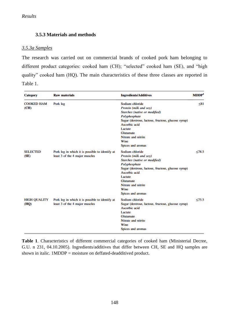
Results
148
3.5.3 Materials and methods
3.5.3a Samples
The research was carried out on commercial brands of cooked pork ham belonging to
different product categories: cooked ham (CH); “selected” cooked ham (SE), and “high
quality” cooked ham (HQ). The main characteristics of these three classes are reported in
Table 1.
Table 1. Characteristics of different commercial categories of cooked ham (Ministerial Decree,
G.U. n 231, 04.10.2005). Ingredients/additives that differ between CH, SE and HQ samples are
shown in italic. 1MDDP = moisture on deffated-deadditived product.
Results
149
In particular, 15 samples (5 for each category) were selected from the Italian market in order
to represent the variety of cooked pork hams available on the Italian market. The set of
samples included: balanced number of samples belonging to the different commercial
category (CH, SE and HQ); samples belonging to the most common Italian brand of cooked
pork ham and presence of samples characterized by different intensities of sensory attribute
(a larger set of samples was evaluated during the training as described in the paragraph
3.5.3b). A sensory description of each product was generated and sensory differences
between products were described and quantified by a panel of highly trained assessors who
have been preselected to have good sensory abilities and received general training as
described in the following section. Moreover, textural and appearance properties (sensory
profiling and instrumental) were measured on the whole set of samples. All cooked hams
(pieces of about 5 kg) were stored at 4 °C, vacuum packed, protected from light, and
physical analysis were carried out in several replicates, whereas for the sensory analysis, the
final score was the average of the scores assigned by each judge to these samples in three
different sessions.
3.5.3b Sensory analysis
Samples were tasted by a panel of 8 expert sensory assessors, balanced in terms of gender,
varying in tasting experience, and previously trained in the assessment of cooked ham. All
of them were regular consumers of cooked ham and interested in the study. Only assessors
who demonstrated specific characteristics such us acuity, ability to communicate and/or to
describe, knowledge of the involved product, interest, motivation and availability to attend
both training and subsequent assessments, were selected. The recruitment, the preliminary
screening and the training were done according to ISO 8586:2012 and ISO 13299:2010. The
performance of selected assessors should be monitored regularly to ensure that the criteria
by which they were initially selected continue to be met. During different sessions, the DA
panel generated a list of appearance, aroma, taste and texture attributes using the consensus
training (Heymann et al., 2014). The training proceeded in 3 sessions: (i) definition of each
descriptor of the sensory vocabulary and the training; in this step the panellists chose a list
of 10 non-overlapping attributes that permit a descriptive analysis of the samples under
Results
150
study and, at the same time, represent an useful tool also for the quality control of the
product; (ii) assessment of the intensity and the memorization of the scale; (iii) sensory
evaluation and monitoring of performance of selected assessors in terms of repeatability,
discriminatory capacity and reproducibility. An agreement on the meaning of the attributes
of the sensory lexicon, must be obtained. For this reason, it is important clearly define
attribute name, written definition, method of assessment and standards reference able to
help judges in the memorization of the different intensity levels for each of the selected
descriptors. After attributes generation, the product assessment protocol must be determined
in order to standardize the procedure and avoid bias. This step includes the way in which the
product needs to be assessed and methods to reset the senses back to a neutral state between
samples. Then, a wide range of samples of a product should be evaluated by rating the
intensity of each attribute on a scale. This training improves the judges ability in using the
sensory scale and promote the use of the ends of the scale. The performance check is
generally carried out by applying statistical treatments to confirm that the panel works in a
consistent and reliable way. The conventional profiling method was applied (Meilgaard et
al., 2007). The final list of descriptors included 3 relative to appearance: typical appearance
(recognition of major muscle), pink intensity (intensity of colour), presence of fat (total
amount of fat inside the slice); 3 perceived by orthonasal and retronasal routes: overall
aroma (intensity of total aroma of the product), spices and flavours (intensity of spices and
other flavours), smoky (aroma associated with smoked notes in meat products); 2 gustatory:
sweet (basic taste), salt (basic taste); 2 relative to the texture: cohesiveness (resistance to the
product separation, to be assessed during the first 3–4 bites), juiciness (amount of juice
released from the product during mastication). Rating of the attribute’s intensities was done
using a linear unstructured 100 mm scale anchored at their extremes (0: absence of
sensation; 100: maximum of sensation intensity) and results were expressed as the mean of
three replicates. Samples were coded with three-random numbers and were presented to the
assessors in randomized blocks. Between samples, a break with water rinses and unsalted
bread sticks was suggested to reduce the carry-over effects as much as possible. To make it
easier to understand and evaluate visual attributes, a group of product images were provided
to each judge as references. These images (anchors) were selected taking into account the
previously results of the training session and were used to illustrate the maximum, the
Results
151
minimum or average intensity points on the scale of typical appearance, pink intensity and
presence of fat. Moreover, in order to standardize the testing conditions as much as possible
and avoid bias, panellists evaluated visual attributes by observing the same slice of product
inside a plate, whereas evaluation of other attributes (smell, taste, and texture) was
performed by providing assessors with a sample minced and placed in plastic cups.
3.5.3c Image analysis
The instrumental measurement of appearance was carried out by an “electronic eye” (visual
analyzer VA400 IRIS, Alpha MOS, France), a high-resolution CCD (charge-coupled
device) camera (resolution 2592 × 1944p) combined with powerful data processing software
(see paragraph 3.4.3d).
3.5.3d Texture analysis
Textural characteristics of HQ, SE, and CH cooked hams were evaluated at 22 °C using a
TA-Hdi® texture analyzer (StableMicro Systems, UK) equipped with a 245 N loading cell.
Texture profile analysis (TPA), Allo-Kramer (AK) shear force, expressible moisture (EM),
and gel strength were assessed in 10 replicates for each sample. TPA, consisting in a double
compression, was run on a 1 cm-high and 2 cm-wide cylindrical-shaped sample compressed
up to 40% of its initial height. The test was performed using a 5 cm-diameter aluminium
probe and a time of 20 sec was elapsed between two compression cycles. Force-time
deformation curves were obtained and hardness (N), springiness, cohesiveness, chewiness
(N), and gumminess (N) were calculated according to Bourne (1978). Shear force test was
performed using an A-K shear cell (10 blades) and a cross-head speed of 500 mm min−1
according to the procedure described by Bianchi et al. (2007). From each cooked ham, a 4 ×
2 × 1 cm sample was excised, weighed, and sheared perpendicularly to the direction of
muscle fibers. Shear force was then calculated as N shear per g of sample. Expressible
moisture (%) was measured following the procedure proposed by Hoffman et al. (1982)
with some modifications. A 4 × 1 × 0.3 cm sample was cut, weighed, and placed between
four filter papers (Whatman No. 1). The sample was compressed through a single
compression cycle with a load of 12.15 N for 5 min and the amount of water released per
gram of meat was calculated, conventionally expressed as percentage. Lastly, gel strength
(N × cm) was assessed on a 1 cm-high and 2 cm-wide cylindrical-shaped sample using a 5
Results
152
mm stainless steel spherical probe according to the procedure described by Petracci et al.
(2009).
3.5.3e Statistical analysis
Instrumental data (AK-shear force, gel strength, expressible moisture, hardness, springiness,
cohesiveness, chewiness, and gumminess) and the intensity of each sensory attribute
(typical appearance, pink intensity, presence of fat, overall aroma, spices and flavours,
smoky, sweet, salt, cohesiveness and juiciness) were analyzed with a one-way-ANOVA or
Kruskal-Wallis (in case of significance of the Levene test) to test the effect of market
category (HQ, SE, and CH). Sensory and physical data were explored by principal
component analysis (PCA). Pearson’s correlations between sensory and instrumental data
were performed to check possible relations. Partial Least Square (PLS) regression was also
applied to predict sensory attributes by instrumental variables. A cross-validation method
was employed to validate PLS models. The precision and the predictive capabilities of the
models were evaluated by the coefficients of determination (R2) and root-mean square error
estimated by cross-validation (RMSECV). All statistical analyses were performed by
XLSTAT 7.5.2 version software (Addinsoft).
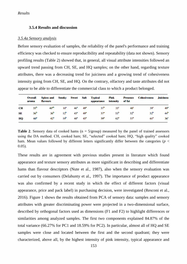
Results
153
3.5.4 Results and discussion
3.5.4a Sensory analysis
Before sensory evaluation of samples, the reliability of the panel's performance and training
efficiency was checked to ensure reproducibility and repeatability (data not shown). Sensory
profiling results (Table 2) showed that, in general, all visual attribute intensities followed an
upward trend passing from CH, SE, and HQ samples; on the other hand, regarding texture
attributes, there was a decreasing trend for juiciness and a growing trend of cohesiveness
intensity going from CH, SE, and HQ. On the contrary, olfactory and taste attributes did not
appear to be able to differentiate the commercial class to which a product belonged.
Table 2. Sensory data of cooked hams (n = 5/group) measured by the panel of trained assessors
using the DA method. CH, cooked ham; SE, “selected” cooked ham; HQ, “high quality” cooked
ham. Mean values followed by different letters significantly differ between the categories (p <
0.05).
These results are in agreement with previous studies present in literature which found
appearance and texture sensory attributes as more significant in describing and differentiate
hams than flavour descriptors (Nute et al., 1987), also when the sensory evaluation was
carried out by consumers (Delahunty et al., 1997). The importance of product appearance
was also confirmed by a recent study in which the effect of different factors (visual
appearance, price and pack label) in purchasing decision, were investigated (Resconi et al.,
2016). Figure 1 shows the results obtained from PCA of sensory data: samples and sensory
attributes with greater discriminating power were projected in a two-dimensional surface,
described by orthogonal factors used as dimensions (F1 and F2) to highlight differences or
similarities among analyzed samples. The first two components explained 84.87% of the
total variance (66.27% for PC1 and 18.59% for PC2). In particular, almost all of HQ and SE
samples were close and located between the first and the second quadrant; they were
characterized, above all, by the highest intensity of pink intensity, typical appearance and
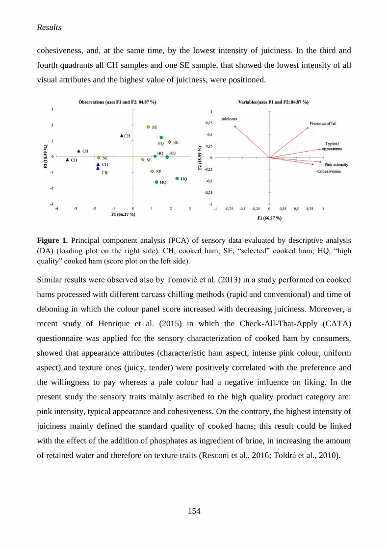
Results
154
cohesiveness, and, at the same time, by the lowest intensity of juiciness. In the third and
fourth quadrants all CH samples and one SE sample, that showed the lowest intensity of all
visual attributes and the highest value of juiciness, were positioned.
Figure 1. Principal component analysis (PCA) of sensory data evaluated by descriptive analysis
(DA) (loading plot on the right side). CH, cooked ham; SE, “selected” cooked ham; HQ, “high
quality” cooked ham (score plot on the left side).
Similar results were observed also by Tomović et al. (2013) in a study performed on cooked
hams processed with different carcass chilling methods (rapid and conventional) and time of
deboning in which the colour panel score increased with decreasing juiciness. Moreover, a
recent study of Henrique et al. (2015) in which the Check-All-That-Apply (CATA)
questionnaire was applied for the sensory characterization of cooked ham by consumers,
showed that appearance attributes (characteristic ham aspect, intense pink colour, uniform
aspect) and texture ones (juicy, tender) were positively correlated with the preference and
the willingness to pay whereas a pale colour had a negative influence on liking. In the
present study the sensory traits mainly ascribed to the high quality product category are:
pink intensity, typical appearance and cohesiveness. On the contrary, the highest intensity of
juiciness mainly defined the standard quality of cooked hams; this result could be linked
with the effect of the addition of phosphates as ingredient of brine, in increasing the amount
of retained water and therefore on texture traits (Resconi et al., 2016; Toldrá et al., 2010).
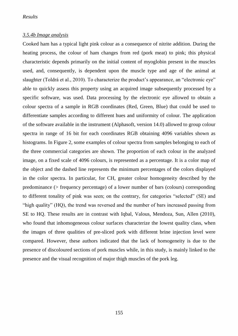
Results
155
3.5.4b Image analysis
Cooked ham has a typical light pink colour as a consequence of nitrite addition. During the
heating process, the colour of ham changes from red (pork meat) to pink; this physical
characteristic depends primarily on the initial content of myoglobin present in the muscles
used, and, consequently, is dependent upon the muscle type and age of the animal at
slaughter (Toldrá et al., 2010). To characterize the product’s appearance, an “electronic eye”
able to quickly assess this property using an acquired image subsequently processed by a
specific software, was used. Data processing by the electronic eye allowed to obtain a
colour spectra of a sample in RGB coordinates (Red, Green, Blue) that could be used to
differentiate samples according to different hues and uniformity of colour. The application
of the software available in the instrument (Alphasoft, version 14.0) allowed to group colour
spectra in range of 16 bit for each coordinates RGB obtaining 4096 variables shown as
histograms. In Figure 2, some examples of colour spectra from samples belonging to each of
the three commercial categories are shown. The proportion of each colour in the analyzed
image, on a fixed scale of 4096 colours, is represented as a percentage. It is a color map of
the object and the dashed line represents the minimum percentages of the colors displayed
in the color spectra. In particular, for CH, greater colour homogeneity described by the
predominance (> frequency percentage) of a lower number of bars (colours) corresponding
to different tonality of pink was seen; on the contrary, for categories “selected” (SE) and
“high quality” (HQ), the trend was reversed and the number of bars increased passing from
SE to HQ. These results are in contrast with Iqbal, Valous, Mendoza, Sun, Allen (2010),
who found that inhomogeneous colour surfaces characterize the lowest quality class, when
the images of three qualities of pre-sliced pork with different brine injection level were
compared. However, these authors indicated that the lack of homogeneity is due to the
presence of discoloured sections of pork muscles while, in this study, is mainly linked to the
presence and the visual recognition of major thigh muscles of the pork leg.
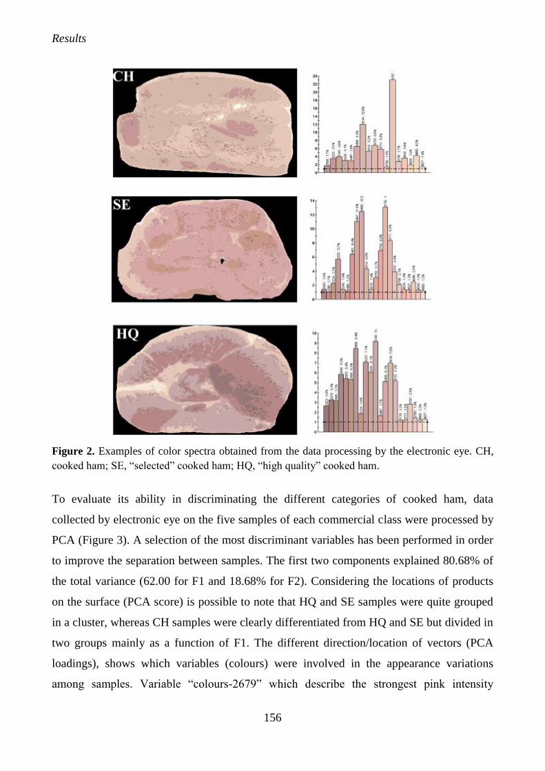
Results
156
Figure 2. Examples of color spectra obtained from the data processing by the electronic eye. CH,
cooked ham; SE, “selected” cooked ham; HQ, “high quality” cooked ham.
To evaluate its ability in discriminating the different categories of cooked ham, data
collected by electronic eye on the five samples of each commercial class were processed by
PCA (Figure 3). A selection of the most discriminant variables has been performed in order
to improve the separation between samples. The first two components explained 80.68% of
the total variance (62.00 for F1 and 18.68% for F2). Considering the locations of products
on the surface (PCA score) is possible to note that HQ and SE samples were quite grouped
in a cluster, whereas CH samples were clearly differentiated from HQ and SE but divided in
two groups mainly as a function of F1. The different direction/location of vectors (PCA
loadings), shows which variables (colours) were involved in the appearance variations
among samples. Variable “colours-2679” which describe the strongest pink intensity
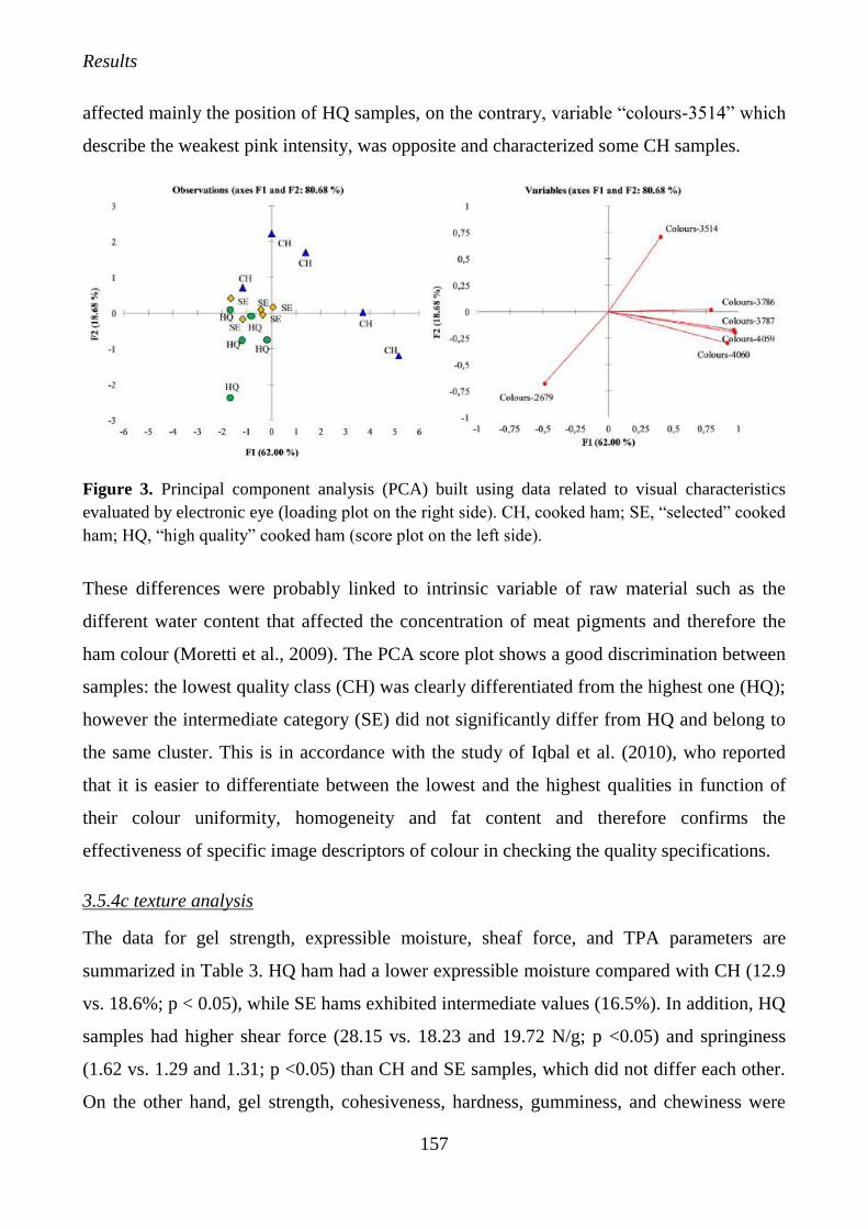
Results
157
affected mainly the position of HQ samples, on the contrary, variable “colours-3514” which
describe the weakest pink intensity, was opposite and characterized some CH samples.
Figure 3. Principal component analysis (PCA) built using data related to visual characteristics
evaluated by electronic eye (loading plot on the right side). CH, cooked ham; SE, “selected” cooked
ham; HQ, “high quality” cooked ham (score plot on the left side).
These differences were probably linked to intrinsic variable of raw material such as the
different water content that affected the concentration of meat pigments and therefore the
ham colour (Moretti et al., 2009). The PCA score plot shows a good discrimination between
samples: the lowest quality class (CH) was clearly differentiated from the highest one (HQ);
however the intermediate category (SE) did not significantly differ from HQ and belong to
the same cluster. This is in accordance with the study of Iqbal et al. (2010), who reported
that it is easier to differentiate between the lowest and the highest qualities in function of
their colour uniformity, homogeneity and fat content and therefore confirms the
effectiveness of specific image descriptors of colour in checking the quality specifications.
3.5.4c texture analysis
The data for gel strength, expressible moisture, sheaf force, and TPA parameters are
summarized in Table 3. HQ ham had a lower expressible moisture compared with CH (12.9
vs. 18.6%; p < 0.05), while SE hams exhibited intermediate values (16.5%). In addition, HQ
samples had higher shear force (28.15 vs. 18.23 and 19.72 N/g; p <0.05) and springiness
(1.62 vs. 1.29 and 1.31; p <0.05) than CH and SE samples, which did not differ each other.
On the other hand, gel strength, cohesiveness, hardness, gumminess, and chewiness were
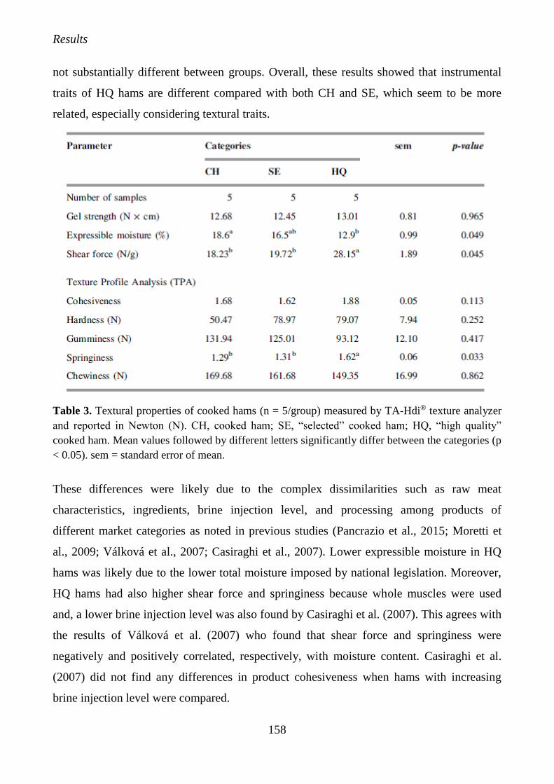
Results
158
not substantially different between groups. Overall, these results showed that instrumental
traits of HQ hams are different compared with both CH and SE, which seem to be more
related, especially considering textural traits.
Table 3. Textural properties of cooked hams (n = 5/group) measured by TA-Hdi® texture analyzer
and reported in Newton (N). CH, cooked ham; SE, “selected” cooked ham; HQ, “high quality”
cooked ham. Mean values followed by different letters significantly differ between the categories (p
< 0.05). sem = standard error of mean.
These differences were likely due to the complex dissimilarities such as raw meat
characteristics, ingredients, brine injection level, and processing among products of
different market categories as noted in previous studies (Pancrazio et al., 2015; Moretti et
al., 2009; Válková et al., 2007; Casiraghi et al., 2007). Lower expressible moisture in HQ
hams was likely due to the lower total moisture imposed by national legislation. Moreover,
HQ hams had also higher shear force and springiness because whole muscles were used
and, a lower brine injection level was also found by Casiraghi et al. (2007). This agrees with
the results of Válková et al. (2007) who found that shear force and springiness were
negatively and positively correlated, respectively, with moisture content. Casiraghi et al.
(2007) did not find any differences in product cohesiveness when hams with increasing
brine injection level were compared.
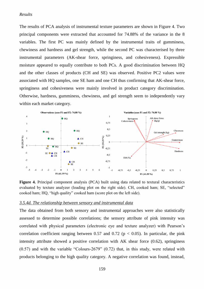
Results
159
The results of PCA analysis of instrumental texture parameters are shown in Figure 4. Two
principal components were extracted that accounted for 74.88% of the variance in the 8
variables. The first PC was mainly defined by the instrumental traits of gumminess,
chewiness and hardness and gel strength, while the second PC was characterised by three
instrumental parameters (AK-shear force, springiness, and cohesiveness). Expressible
moisture appeared to equally contribute to both PCs. A good discrimination between HQ
and the other classes of products (CH and SE) was observed. Positive PC2 values were
associated with HQ samples, one SE ham and one CH thus confirming that AK-shear force,
springiness and cohesiveness were mainly involved in product category discrimination.
Otherwise, hardness, gumminess, chewiness, and gel strength seem to independently vary
within each market category.
Figure 4. Principal component analysis (PCA) built using data related to textural characteristics
evaluated by texture analyzer (loading plot on the right side). CH, cooked ham; SE, “selected”
cooked ham; HQ, “high quality” cooked ham (score plot on the left side).
3.5.4d. The relationship between sensory and instrumental data
The data obtained from both sensory and instrumental approaches were also statistically
assessed to determine possible correlations; the sensory attribute of pink intensity was
correlated with physical parameters (electronic eye and texture analyzer) with Pearson’s
correlation coefficient ranging between 0.57 and 0.72 (p < 0.05). In particular, the pink
intensity attribute showed a positive correlation with AK shear force (0.62), springiness
(0.57) and with the variable “Colours-2679” (0.72) that, in this study, were related with
products belonging to the high quality category. A negative correlation was found, instead,
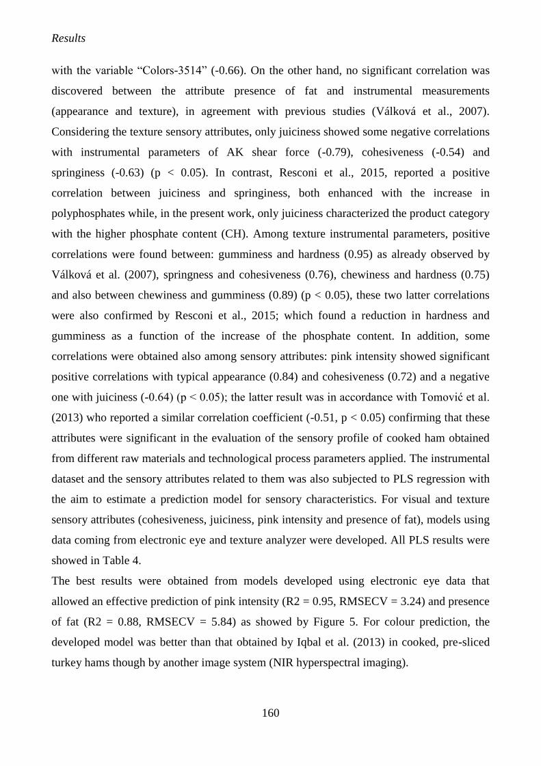
Results
160
with the variable “Colors-3514” (-0.66). On the other hand, no significant correlation was
discovered between the attribute presence of fat and instrumental measurements
(appearance and texture), in agreement with previous studies (Válková et al., 2007).
Considering the texture sensory attributes, only juiciness showed some negative correlations
with instrumental parameters of AK shear force (-0.79), cohesiveness (-0.54) and
springiness (-0.63) (p < 0.05). In contrast, Resconi et al., 2015, reported a positive
correlation between juiciness and springiness, both enhanced with the increase in
polyphosphates while, in the present work, only juiciness characterized the product category
with the higher phosphate content (CH). Among texture instrumental parameters, positive
correlations were found between: gumminess and hardness (0.95) as already observed by
Válková et al. (2007), springness and cohesiveness (0.76), chewiness and hardness (0.75)
and also between chewiness and gumminess (0.89) (p < 0.05), these two latter correlations
were also confirmed by Resconi et al., 2015; which found a reduction in hardness and
gumminess as a function of the increase of the phosphate content. In addition, some
correlations were obtained also among sensory attributes: pink intensity showed significant
positive correlations with typical appearance (0.84) and cohesiveness (0.72) and a negative
one with juiciness (-0.64) (p < 0.05); the latter result was in accordance with Tomović et al.
(2013) who reported a similar correlation coefficient (-0.51, p < 0.05) confirming that these
attributes were significant in the evaluation of the sensory profile of cooked ham obtained
from different raw materials and technological process parameters applied. The instrumental
dataset and the sensory attributes related to them was also subjected to PLS regression with
the aim to estimate a prediction model for sensory characteristics. For visual and texture
sensory attributes (cohesiveness, juiciness, pink intensity and presence of fat), models using
data coming from electronic eye and texture analyzer were developed. All PLS results were
showed in Table 4.
The best results were obtained from models developed using electronic eye data that
allowed an effective prediction of pink intensity (R2 = 0.95, RMSECV = 3.24) and presence
of fat (R2 = 0.88, RMSECV = 5.84) as showed by Figure 5. For colour prediction, the
developed model was better than that obtained by Iqbal et al. (2013) in cooked, pre-sliced
turkey hams though by another image system (NIR hyperspectral imaging).
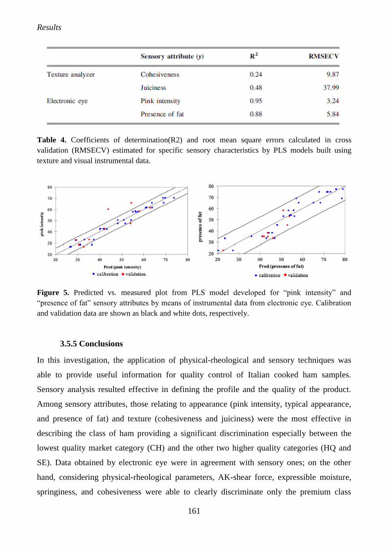
Results
161
Table 4. Coefficients of determination(R2) and root mean square errors calculated in cross
validation (RMSECV) estimated for specific sensory characteristics by PLS models built using
texture and visual instrumental data.
Figure 5. Predicted vs. measured plot from PLS model developed for “pink intensity” and
“presence of fat” sensory attributes by means of instrumental data from electronic eye. Calibration
and validation data are shown as black and white dots, respectively.
3.5.5 Conclusions
In this investigation, the application of physical-rheological and sensory techniques was
able to provide useful information for quality control of Italian cooked ham samples.
Sensory analysis resulted effective in defining the profile and the quality of the product.
Among sensory attributes, those relating to appearance (pink intensity, typical appearance,
and presence of fat) and texture (cohesiveness and juiciness) were the most effective in
describing the class of ham providing a significant discrimination especially between the
lowest quality market category (CH) and the other two higher quality categories (HQ and
SE). Data obtained by electronic eye were in agreement with sensory ones; on the other
hand, considering physical-rheological parameters, AK-shear force, expressible moisture,
springiness, and cohesiveness were able to clearly discriminate only the premium class
Results
162
(“high quality”) from each other. The electronic eye applied in this study allowed to develop
a PLS models with a promising value of prediction of visual attribute of presence of fat and
pink intensity (R2 = 0.88, RMSECV = 5.84 and R2 = 0.95, RMSECV = 3.24, respectively).
Based on these preliminary results, the use of physical-rheological parameters could be
proposed to complement sensory analysis, for example in the definition of reference
standards and for rapid quality control of different categories and classes of the same
product. This study permitted to hypothesize a preliminary model for a fast and effective
screenings to be conducted by a “one-day” experimental plan suitable for the quality control
also of other categories of meat products. This analytical approach could be particularly
interesting for food providers, buyers and retailers that intend to protect and promote these
products to better addressing consumer needs and enhancing their competitiveness on the
market. However, further efforts aimed to differentiate and certify a higher quality product
and to improve consumer's knowledge and to direct them towards a more informed choice,
are needed. Work in progress includes a consumer study on cooked pork hams to investigate
the correspondence between attributes generated by the panel and consumer lexicon used in
quality-related communications.
3.5.6 Aknowledgements
This study could not have been realized without the precious help of COOP ITALIA and
NEGRINI SALUMI as the main suppliers of the samples used herein.
This work was supported by the Italian program FARB – Financing of Alma Mater
Studiorum – University of Bologna for basic research. Line of Action 2 – Project Meating
“sensory and fast instrumental analyses of meat and meat products: an integrated approach
for quality control and communication.”.
Results
163
3.5.7 References
Aaslyng M.D. 2002. Quality indicators for raw meat. In: Kerry, J.K., Kerry, J., Ledward, D.
(Eds.), Meat Processing: Improving Quality. CRC Press, Boca Raton, FL, pp. 157–174.
ASSICA. 2014. Associazione Industriali delle Carni e dei Salumi, annual report. Available
from http://www.assica.it.
Bianchi M., Petracci M., Pascual M., Cavani C. 2007. Comparison between Allo-Kramer and
Warner-Bratzler devices to assess rabbit meat tenderness. Italial Journal of Animal Science,
6, 749–751.
Bourne M.C. 1978. Texture profile analysis. Food Technology, 32, 62–66.
Brosnan T., Sun D.W. 2004. Improving quality inspection of food products by computer
vision: a review. Journal of Food Engineering, 61, 3–16.
Casiraghi E., Alamprese C., Pompei C. 2007. Cooked ham classification on the basis of brine
in jection level and pork breeding country. Food Science and Technology, 40, 164–169.
Delahunty C.M., McCord A., O’Neill E.E., Morrissey P.A. 1997. Sensory characterization of
cooked ham by untrained consumers using free-choice profiling. Food Quality and
Preference, 8, 381–388.
Desmond E.M., Kenny T.A., Ward P., Sun D.W. 2000. Effect of rapid and conventional
cooling methods on the quality of cooked ham joints. Meat Science, 56, 271–277.
ElMasry G., Sun D.-W., Allen P. 2012. Near-infrared hyperspectral imaging for predicting
colour, pH and tenderness of fresh beef. Journal of Food Engineering, 110, 127–140.
Fongaro L., Alamprese C., Casiraghi E. 2015. Ripening of salami: assessment of colour and
aspect evolution using image analysis and multivariate image analysis. Meat Science 101,
73–77.
Heinz G., Hautzinger P. 2007. Meat processing technology for small-to medium scale
producers. Food and Agriculture Organization of the United Nations. Regional office for
Asia and the pacific RAP publication, Bangkok 2007/20.
Henrique N.A., Deliza R., Rosenthal A. 2015. Consumer sensory characterization of cooked
ham using the check-all-that-apply (CATA) methodology. Food Engineering Review, 7,
265–273.
Results
164
Heymann H., King E.S., Hopfer H. 2014. Classical descriptive analysis, In: Varela P., Ares
G., (Eds.), Novel Techniques in Sensory Characterization and Consumer Profiling, CRC
Press; Boca Raton, FL, 9–36.
Hoffman K., Hamm R., Bluchel E. 1982. Neues uber die bestimmung der wasserbindung des
fleisches mit hilfe der filterpapierpremethode. Fleischwirtsch, 62, 87–92.
Iqbal A., Sun D.W., Allen P. 2013. Prediction of moisture, color and pH in cooked, pre-sliced
turkey hams by NIR hyperspectral imaging system. Journal of Food Engineering, 117, 42–
51.
Iqbal A., Sun D.W., Allen P. 2014. An overview on principle: techniques and application of
hyperspectral imaging with special reference to ham quality evaluation and control. Food
Control, 46, 242–254.
Iqbal A., Valous N.A., Mendoza F., Sun D.-W., Allen P. 2010. Classification of pre-sliced
pork and Turkey ham qualities based on image colour and textural features and their
relationships with consumer responses. Meat Science, 84, 455–465.
ISO (International Organization for Standardization) EN ISO 13299:2010. Sensory analysis –
Methodology – General guidance for establishing a sensory profile.
ISO (International Organization for Standardization) ISO 8586:2012 (E). Sensory analysis –
General guidelines for the selection, training and monitoring of selected assessors and
expert sensory assessors.
Martinez O., Salmerón J., Guillén M.D., Casas C. 2004. Texture profile analysis of meat
products treated with commercial liquid smoke flavourings, Food Control, 15, 457–461.
Meilgaard M.C., Civille G.V., Carr B.T. 2007. Descriptive analysis techniques, In: Meilgaard
M.C., Civille G.V., Carr B.T., (Eds.). Sensory Evaluation Techniques, CRC Press; Boca
Raton, FL, 173–188.
Ministerial Decree, G.U. n 231, 04/10/2005 Regulation of the production and selling of
specific meat products.
Moretti V.M., Bellagamba F., Paleari M.A., Beretta G., Busetto M.L., Caprino F. 2009.
Differentiation of cured cooked hams by physico-chemical properties and chemometrics.
Journal of Food Quality, 32, 2009, 125–140.
Results
165
Nute G.R., Jones R.C.D., Dransfield E., Whelehan P. 1987. Sensory characteristics of ham
and their relationships with composition, visco-elasticity and strength. International Journal
of Food Science and Technology, 22, 461–476.
Pancrazio G., Cunha S.C., De Pinho P.G., Loureiro M., Ferreira I., Pinho O. 2015. Physical
and chemical characteristics of cooked ham: effect of tumbling time and modifications
during storage. Journal of Food Quality, 38, 359–368.
Petracci M., Bianchi M., Franchini A., Cavani C. Technological characteristics of turkey
breast rolls produced with fresh or thawed meat and different formulations, In: Proceedings
of the 19th European Symposium on Quality of Poultry Meat, Turku, Finland, 21–25 June
2009.
Resconi V.C., Keenan D.F., Barahona M., Guerrero L., Kerry J.P., Hamill R.M. 2016. Rice
starch and fructo-oligosaccharides as substitutes for phosphate and dextrose in whole
muscle cooked hams: sensory analysis and consumer preferences. Food Science and
Technology, 66, 284–292.
Resconi V.C., Keenan D.F., Gough S., Doran L., Allen P., Kerry J.P., Hamill R.M. 2015.
Response surface methodology analysis of rice starch and fructooligosaccharides as
substitutes for phosphate and dextrose in whole muscle cooked hams. Food Science and
Technology, 64, 946–958.
Sánchez A.J., Albarracin W., Grau R., Ricolfe C., Barat J.M., Control of ham salting by using
image segmentation. Food Control, 19, 135–142.
Toldrá F., Mora L., Flores M., Cooked ham, In: Toldrá F., (Ed), Handbook of Meat
Processing, 2010, Wiley-Blackwell; Ames, IA, 299–311.
Tomović V.M., Jokanović M.R., Petroović L.S., Tomović M.S., Tasić T.A., Ikonić P.M.,
Sŭmić Z.M., Šojić B.V., Škaljac S.B., Šošo M.M. 2013. Sensory: physical and chemical
characteristics of cooked ham manufactured from rapidly chilled and earlier deboned M.
semimembranosus. Meat Science, 93, 46–52.
Válková V., Saláková A., Buchtová H., Tremlová B. 2007. Chemical: instrumental and
sensory characteristics of cooked pork ham. Meat Science, 77, 608–615.
Results
166
3.6 Children preferences of coloured cheese prepared during an educational
laboratory
Publication details:
Title: Children preferences of coloured cheese prepared during an educational laboratory
Authors: Tesini F1, Laureati M2, Palagano R1, Mandrioli M1, Pagliarini E2, Gallina Toschi T1,3 1DISTAL, Department of Agricultural and Food Sciences, Alma Mater Studiorum, University of
Bologna, P.zza Goidanich 60, 47521 Cesena, FC, Italy 2Department of Food, Environmental and Nutritional Sciences (DeFENS), University of Milan, Via
Celoria 2, 20133Milan, Italy 3CIRI, Interdepartmental Centre for Industrial Grifood Research, Alma Mater Studiorum,
University of Bologna, P.zza Goidanich 60, 47521 Cesena, FC, Italy
Published on: Italian Journal of Food Science. 2015. 27, 521-526
3.6.1 Abstract
Choices among young consumers are mainly driven by food preferences; in particular, a
connection between appearance and acceptance of food has been highlighted, together with
a general lack of knowledge of food processing. For these reasons, educational activities are
important to increase scientific knowledge and awareness. The cheese-making educational
laboratory described herein involved children, adolescents, and their parents/teachers in the
preparation of fresh and naturally-coloured cheeses. At the end of the activity, both the
colour preference and possible relation between preference and colour of cheese prepared
were investigated administering a short questionnaire.
Keywords: cheese preference; children food preference; colour preference; gender;
neophobia; nutrition education.
Results
167
3.6.2 Introduction
Food preference has a fundamental role in driving consumer’s choices and habits, especially
in children (Laureati et al., 2015a; Cooke, 2007; Nicklaus et al., 2004). Therefore, the
number of food products specifically developed for children is growing and this market is
acquiring increasing importance (Issanchou, 2015). Consequently, the youngest consumers
are frequently involved in research and development programs, since their food habits will
influence choices as they grow older and because their preferences, even if partly driven by
advertisements (Ustjanauskas et al., 2014), seem to be strictly related to the sensory aspects
of food (Mustonen and Tuorila, 2010; Pagliarini et al., 2005). In 1994, Moskowitz
(Moskowits, 1994) highlighted how a visually pleasing product tends to be more
appreciated by children, as visual attributes seem to be, among different sensory
characteristics, those that mainly determine its success (Topcu, 2015; Kildegaard et al.,
2011). Indeed, children tend to create an “ideal picture” of each food product that can be
related to their own idea of “good”; this picture represent a sort of reference point that can
be used to dislike products whose appearance is not close to their expectation (Mustonen et
al., 2009). This phenomenon, called food neophobia, is defined as the fear of eating new or
unfamiliar food (Pliner et al., 1992) and is related to both the quality and variety of diet
(Laureati et al., 2015b). Nutritional education and food-related diseases prevention activities
can be used for children and teenagers in order to: i) reduce the impact of poor food habits
on health, and ii) avoid food neophobia, mainly responsible for refusing consumption of
fruits and vegetables (Wardle et al., 2003). Moreover, a lack of awareness of procedural
knowledge, both in terms of food processing and nutritional values, must be taken into
account (Worsley, 2002), highlighting the link between traditional food preparation and
sensory properties (Laureati et al., 2006). Nowadays, food education is mainly based on the
social-cognitive theory (SCT) (Bandura et al., 1977), which incorporates the interaction of
personal, environmental and behavioural factors. According to this theory, principles that
are highly influential in establishing changing food behaviour in children are both models
and repeated exposure. Among the models, those that have been found to be effective in
children include cartoon characters, peers, mothers, unfamiliar adults and teachers;
moreover, children seem to be influenced more by the behaviour of multiple rather than
single models (Lowe et al., 2004). Furthermore, according to Zajonc’s “mere exposure”
Results
168
theory (Zajonc, 1968), repeated exposure to a specific food increases the liking and
consumption of that food (Cooke et al., 2011; Wardle et al., 2003b) through a mechanism
that is believed to be a “learned safety” behaviour (Kalat et al., 1973). According to this
theory, repeated ingestion of an unfamiliar food without negative consequences leads to
increased acceptance of that food. Several educational interventions for food have
investigated all these factors, reporting promising results, especially for consumption of
fruits and vegetables (Laureati et al., 2014; Evans et al., 2012; Reverdy et al., 2008). Both
principles of imitation and repeated exposure characterise food laboratories aimed at
involving children in food preparation, thus familiarising them with food ingredients and
technologies. Furthermore, it has been reported that the involvement of children in food
preparation can contribute to increasing their acceptance for that food, according to the
principle of repeated exposure (Chu et al., 2012). For all these reasons, food educational
interventions can play a relevant role in driving choice, interest and preference of children
through better awareness of both sensory characteristics and technological process of
traditional food products (Mustonen et al., 2010). The educational cheese-making activity
reported herein, called Cheese making in one hour, was conceived by a committee of
referees as part of the Festival della Scienza 2014 (which took place in Genoa, Italy, from
October 24 to November 2, 2014) and is considered as a “teaching tool” in order to increase
scientific information about the cheese-making process. This practical laboratory took the
form of a family entertainment during which children and parents or teachers could share
principles of traditional cheese making, spending some family or educational time away
from daily work, but related to increased knowledge of food science. The activity involved
children, teenagers and adults (age from 6 to 87 years) in the traditional preparation of a
fresh “primo sale like” cheese. Cheeses were naturally coloured (using turmeric, rocket and
beetroot juice), and in order to keep the attention of participants, each was actively involved
in the process by preparing his/her personal small cheese. At the end of the activity, both the
colour preference and possible relation between the colour of cheese prepared and
preference were investigated by administration of a short and simple questionnaire.
Results
169
3.6.3 Materials and methods
The cheese-making activity involved 738 participants (395 females and 343 males) with an
age between 5 and 87 years and divided in groups of no more than 30 individuals. Both
families and school classes could participate in the activity by asking the Festival staff to
make a reservation; given the popularity of the Festival, mainly represented by children and
partly by parents/teachers, a large number of participants were enrolled. Each participant
had an active role in the laboratory, giving his/her contribution to one of the four phases of
cheese making: 1) adding starter, rennet and natural flavour to milk; 2) curd cutting and
synaeresis; 3) curd breaking and purge; 4) cheese shaping. During the Festival, the
laboratory was repeated at least 3 times a day by 4 previously-trained scientific facilitators.
Due to the fact that the cheese-making laboratory should last only one hour (related to the
timing of the Festival), one pot (Bartscher GmbH, Germany) was dedicated to each of the 4
main phases; in this way, participants could move from one pot to the next instead of
proceeding step-by-step using a single pot such that each of the phases could be observed in
a short length of time.
3.6.3a Cheese-making phases
Starter, rennet and milk natural flavouring. Fresh whole cow milk was heated to 36° C
and 17 g/L of natural whole yoghurt was added as a starter. In order to produce coloured
cheeses, different natural dyes were added (rocket, turmeric and beetroot juice) as reported
in Table 1. While turmeric and beetroot juice were added to the milk 30 minutes after the
addition of starter, together with 0.5 mL/l milk of liquid rennet (80% chymosin, 20%
pepsin, provided by Graco), rocket was added during the last step of cheese shaping.
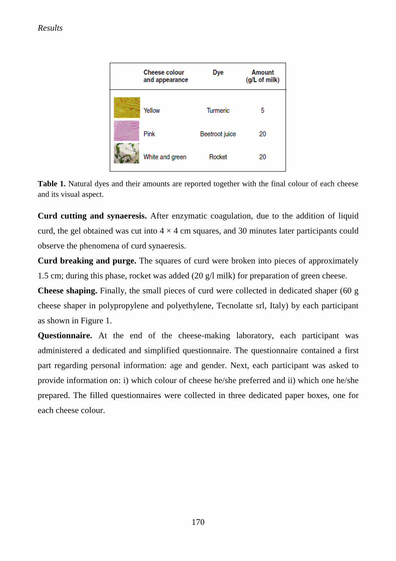
Results
170
Table 1. Natural dyes and their amounts are reported together with the final colour of each cheese
and its visual aspect.
Curd cutting and synaeresis. After enzymatic coagulation, due to the addition of liquid
curd, the gel obtained was cut into 4 × 4 cm squares, and 30 minutes later participants could
observe the phenomena of curd synaeresis.
Curd breaking and purge. The squares of curd were broken into pieces of approximately
1.5 cm; during this phase, rocket was added (20 g/l milk) for preparation of green cheese.
Cheese shaping. Finally, the small pieces of curd were collected in dedicated shaper (60 g
cheese shaper in polypropylene and polyethylene, Tecnolatte srl, Italy) by each participant
as shown in Figure 1.
Questionnaire. At the end of the cheese-making laboratory, each participant was
administered a dedicated and simplified questionnaire. The questionnaire contained a first
part regarding personal information: age and gender. Next, each participant was asked to
provide information on: i) which colour of cheese he/she preferred and ii) which one he/she
prepared. The filled questionnaires were collected in three dedicated paper boxes, one for
each cheese colour.
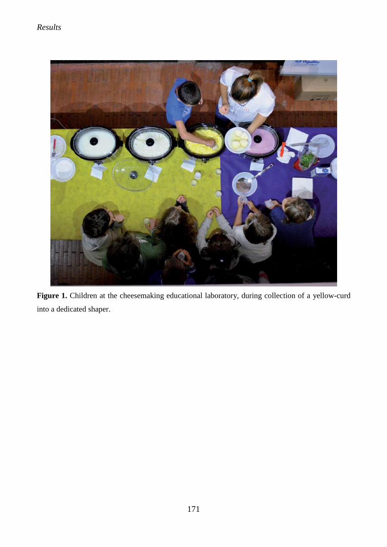
Results
171
Figure 1. Children at the cheesemaking educational laboratory, during collection of a yellow-curd
into a dedicated shaper.
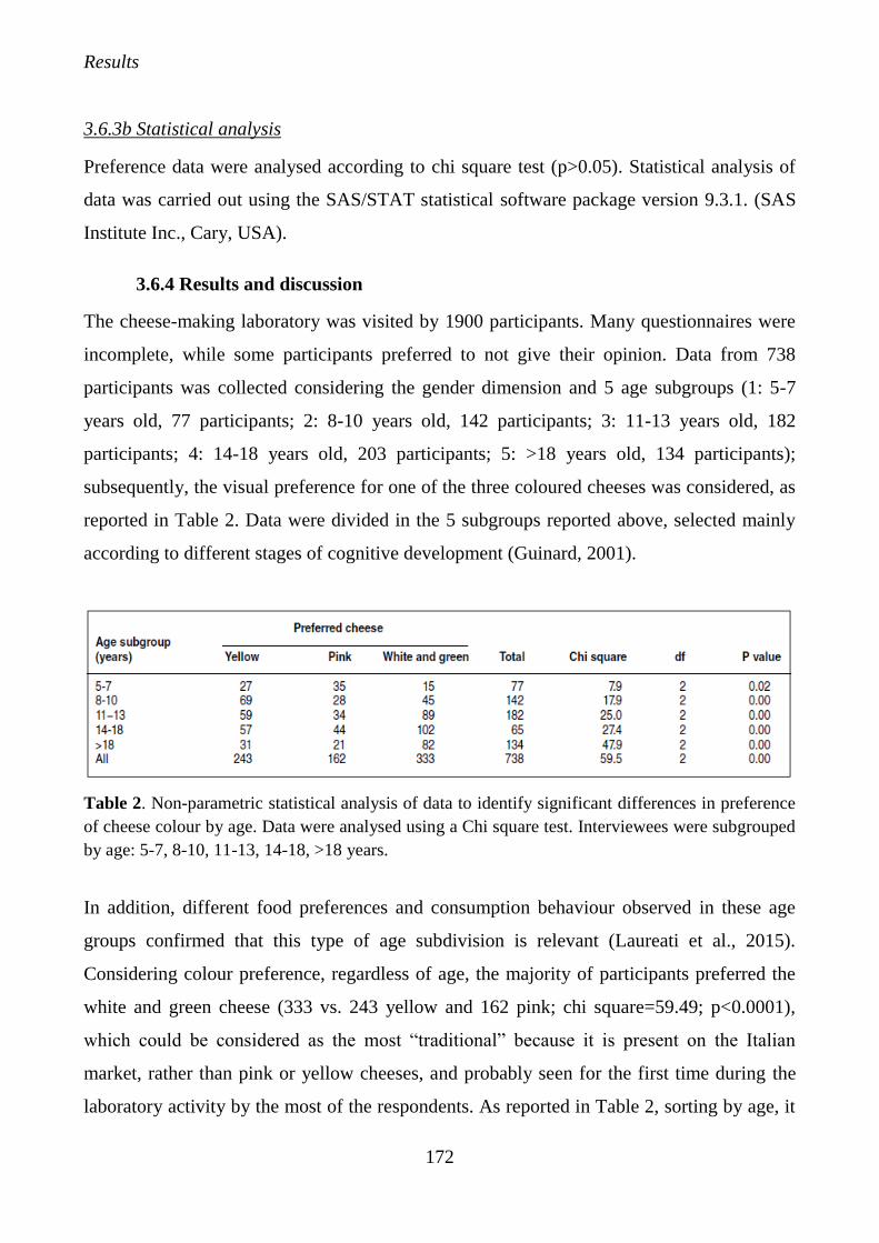
Results
172
3.6.3b Statistical analysis
Preference data were analysed according to chi square test (p>0.05). Statistical analysis of
data was carried out using the SAS/STAT statistical software package version 9.3.1. (SAS
Institute Inc., Cary, USA).
3.6.4 Results and discussion
The cheese-making laboratory was visited by 1900 participants. Many questionnaires were
incomplete, while some participants preferred to not give their opinion. Data from 738
participants was collected considering the gender dimension and 5 age subgroups (1: 5-7
years old, 77 participants; 2: 8-10 years old, 142 participants; 3: 11-13 years old, 182
participants; 4: 14-18 years old, 203 participants; 5: >18 years old, 134 participants);
subsequently, the visual preference for one of the three coloured cheeses was considered, as
reported in Table 2. Data were divided in the 5 subgroups reported above, selected mainly
according to different stages of cognitive development (Guinard, 2001).
Table 2. Non-parametric statistical analysis of data to identify significant differences in preference
of cheese colour by age. Data were analysed using a Chi square test. Interviewees were subgrouped
by age: 5-7, 8-10, 11-13, 14-18, >18 years.
In addition, different food preferences and consumption behaviour observed in these age
groups confirmed that this type of age subdivision is relevant (Laureati et al., 2015).
Considering colour preference, regardless of age, the majority of participants preferred the
white and green cheese (333 vs. 243 yellow and 162 pink; chi square=59.49; p<0.0001),
which could be considered as the most “traditional” because it is present on the Italian
market, rather than pink or yellow cheeses, and probably seen for the first time during the
laboratory activity by the most of the respondents. As reported in Table 2, sorting by age, it
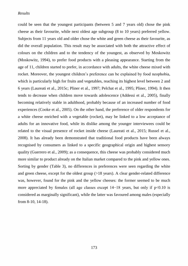
Results
173
could be seen that the youngest participants (between 5 and 7 years old) chose the pink
cheese as their favourite, while next oldest age subgroup (8 to 10 years) preferred yellow.
Subjects from 11 years old and older chose the white and green cheese as their favourite, as
did the overall population. This result may be associated with both the attractive effect of
colours on the children and to the tendency of the youngest, as observed by Moskowitz
(Moskowitz, 1994), to prefer food products with a pleasing appearance. Starting from the
age of 11, children started to prefer, in accordance with adults, the white cheese mixed with
rocket. Moreover, the youngest children’s preference can be explained by food neophobia,
which is particularly high for fruits and vegetables, reaching its highest level between 2 and
6 years (Laureati et al., 2015c; Pliner et al., 1997; Pelchat et al., 1995; Pliner, 1994). It then
tends to decrease when children move towards adolescence (Addessi et al., 2005), finally
becoming relatively stable in adulthood, probably because of an increased number of food
experiences (Cooke et al., 2005). On the other hand, the preference of older respondents for
a white cheese enriched with a vegetable (rocket), may be linked to a low acceptance of
adults for an innovative food, while its dislike among the younger interviewees could be
related to the visual presence of rocket inside cheese (Laureati et al., 2015; Russel et al.,
2008). It has already been demonstrated that traditional food products have been always
recognised by consumers as linked to a specific geographical origin and highest sensory
quality (Guerrero et al., 2009); as a consequence, this cheese was probably considered much
more similar to product already on the Italian market compared to the pink and yellow ones.
Sorting by gender (Table 3), no differences in preferences were seen regarding the white
and green cheese, except for the oldest group (>18 years). A clear gender-related difference
was, however, found for the pink and the yellow cheeses: the former seemed to be much
more appreciated by females (all age classes except 14−18 years, but only if p<0.10 is
considered as marginally significant), while the latter was favoured among males (especially
from 8-10, 14-18).
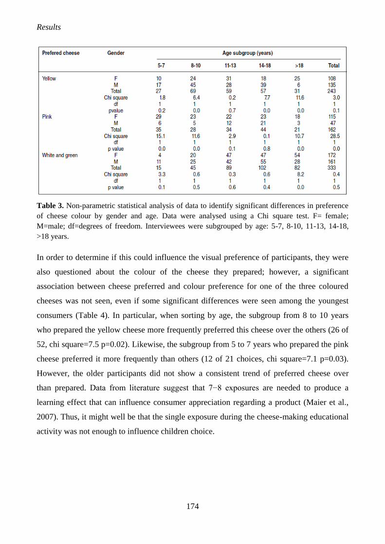
Results
174
Table 3. Non-parametric statistical analysis of data to identify significant differences in preference
of cheese colour by gender and age. Data were analysed using a Chi square test. F= female;
M=male; df=degrees of freedom. Interviewees were subgrouped by age: 5-7, 8-10, 11-13, 14-18,
>18 years.
In order to determine if this could influence the visual preference of participants, they were
also questioned about the colour of the cheese they prepared; however, a significant
association between cheese preferred and colour preference for one of the three coloured
cheeses was not seen, even if some significant differences were seen among the youngest
consumers (Table 4). In particular, when sorting by age, the subgroup from 8 to 10 years
who prepared the yellow cheese more frequently preferred this cheese over the others (26 of
52, chi square=7.5 p=0.02). Likewise, the subgroup from 5 to 7 years who prepared the pink
cheese preferred it more frequently than others (12 of 21 choices, chi square=7.1 p=0.03).
However, the older participants did not show a consistent trend of preferred cheese over
than prepared. Data from literature suggest that 7−8 exposures are needed to produce a
learning effect that can influence consumer appreciation regarding a product (Maier et al.,
2007). Thus, it might well be that the single exposure during the cheese-making educational
activity was not enough to influence children choice.
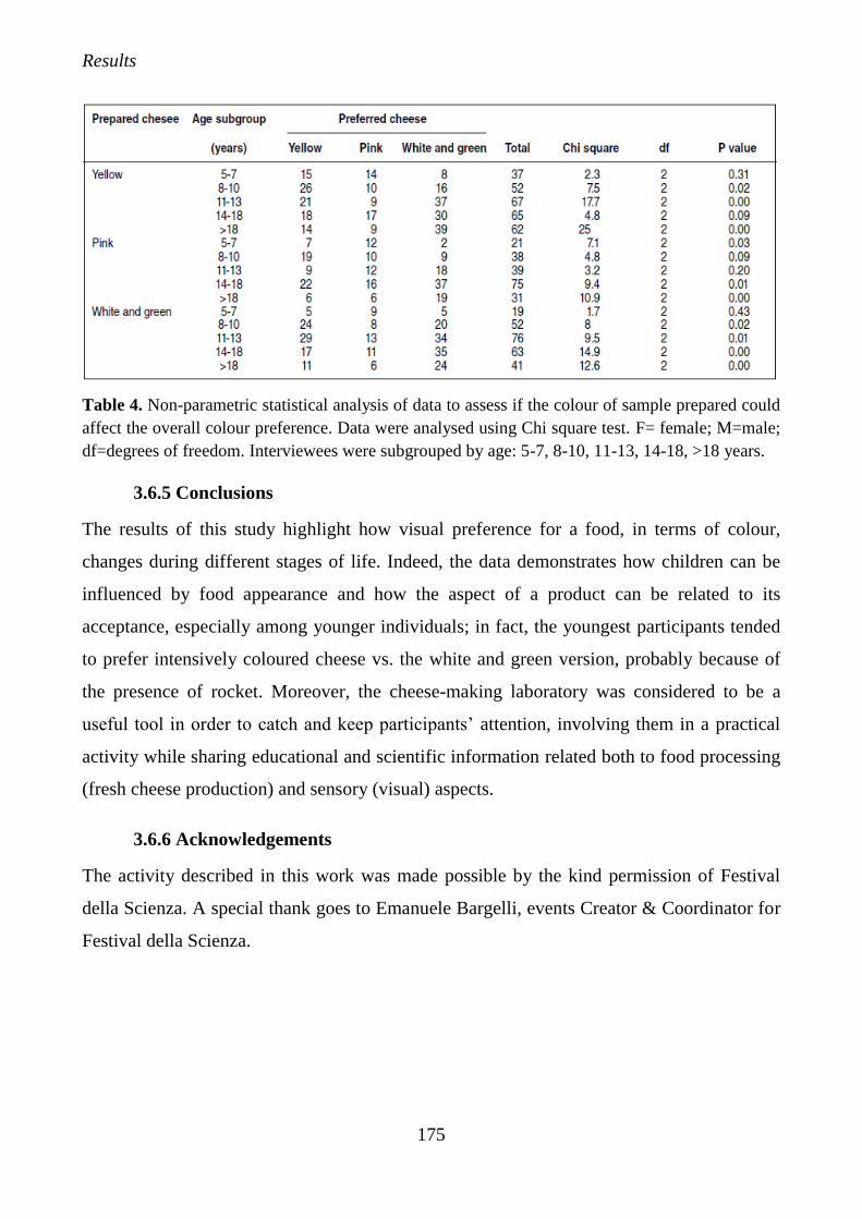
Results
175
Table 4. Non-parametric statistical analysis of data to assess if the colour of sample prepared could
affect the overall colour preference. Data were analysed using Chi square test. F= female; M=male;
df=degrees of freedom. Interviewees were subgrouped by age: 5-7, 8-10, 11-13, 14-18, >18 years.
3.6.5 Conclusions
The results of this study highlight how visual preference for a food, in terms of colour,
changes during different stages of life. Indeed, the data demonstrates how children can be
influenced by food appearance and how the aspect of a product can be related to its
acceptance, especially among younger individuals; in fact, the youngest participants tended
to prefer intensively coloured cheese vs. the white and green version, probably because of
the presence of rocket. Moreover, the cheese-making laboratory was considered to be a
useful tool in order to catch and keep participants’ attention, involving them in a practical
activity while sharing educational and scientific information related both to food processing
(fresh cheese production) and sensory (visual) aspects.
3.6.6 Acknowledgements
The activity described in this work was made possible by the kind permission of Festival
della Scienza. A special thank goes to Emanuele Bargelli, events Creator & Coordinator for
Festival della Scienza.
Results
176
3.6.7 References
Addessi E., Galloway A.T., Visalberghi E., Birch L.L. 2005. Specific social influences on the
acceptance of novel foods in 2–5-year-old children. Appetite ,45, 264.
Bandura A., Adams N.E. 1977. Analysis of self-efficacy theory of behavioural change.
Cognitive Therapy and Research, 1, 287.
Chu Y.L., Farmer A., Fung C., Kuhle S., Storey K.E., Veugelers P.J. 2013. Involvement in
home meal preparation is associated with food preference and self-efficacy among Canadian
children. Public Health Nutrition, 16, 108.
Cooke L.,Wardle J. 2005. Age and gender differences in children’s food preferences. British
Journal of Nutrition, 93, 741.
Cooke L. 2007. The importance of exposure for healthy eating in childhood: a review.
Journal of Human Nutrition and Diet, 20, 294.
Cooke L.J., Chambers L.C., Añez E.V., Croker H.A., Boniface D., Yeomans M.R., Wardle J.
2011. Eating for pleasure or profit: the effect of incentives on children’s enjoyment of
vegetables. Psychology Science, 22, 190.
Evans C.E., Christian M.S., Cleghorn C.L., Greenwood D.C., Cade J.E. 2012. Systematic
review and meta-analysis of school-based interventions to improve daily fruit and vegetable
intake in children aged 5 to 12 years. American Journal of Clinical Nutrition, 96, 889.
Galloway A.T., Lee Y., Birch L.L. 2005. Predictors and consequences of food neophobia and
pickiness in young girls. Journal of American Diet Association, 103, 692.
Guerrero L., Guàrdia M.D., Xicola J., Verbeke W., Vanhonacker F., Zakowska-Biemans S.,
Hersleth M. 2009. Consumer-driven definition of traditional food products and innovation
in traditional foods. A qualitative cross-cultural study. Appetite, 52, 345.
Guinard J-X. 2001. Sensory and consumer testing with children. Trends Food Science and
Technology, 11, 273.
Issanchou S. 2015. Sensory & consumer studies with special populations: children and
elderly. Current Opinion in Food Science, 3,53.
Kalat J.W., Rozin P. 1973. “Learned safety” as a mechanism in long-delay taste-aversion
learning in rats. Journal of Comparative and Physiological Psychology, 83, 198.
Results
177
Kildegaard H., Olsen A., Gabrielsen G., Moller P., Thybo A.K. 2011. A method to measure
the effect of food appearance factors on children’s visual preferences. Food Quality and
Preference, 22, 763.
Laureati M., Pagliarini E., Calcinoni O., Bidoglio M. 2006. Sensory acceptability of
traditional food preparations by elderly people. Food Quality and Preference, 17, 43.
Laureati M., Pagliarini E., Toschi T.G., Monteleone E. 2015a. Research challenges and
methods to study food preferences in school-aged children: A review of the last 15 years.
Food Quality and Preference, 46, 92.
Laureati M., Bergamaschi V., Pagliarini E. 2015b. Assessing childhood food neophobia:
Validation of a scale in Italian primary school children. Food Quality and Preference, 40, 8.
Laureati M., Bertoli S., Bergamaschi V., Leone A., Lewandowski L., Giussani B., Battezzati
A., Pagliarini, E. 2015c. Food neophobia and liking for fruits and vegetables are not related
to excess weight in Italian children. Food Quality and Preference, 40, 125.
Lowe C.F., Horne P.J., Tapper K., Bowdery M., Egerton C. 2004. Effects of a peer modelling
and rewards-based intervention to increase fruit and vegetable consumption in children.
European Journal of Clinical Nutrition, 58, 510.
Maier A.S., Chabanet C., Schaal B., Issanchou S., Leathwood P. 2007. Effects of repeated
exposure on acceptance of initially disliked vegetables in 7-month old infants Food Quality
and Preference, 18, 1023.
Moskowitz H.R. 1994. “Food Concepts and Products: Just-intime Development” Food and
Nutrition Press.
Mustonen S., Tuorila H. 2010. Sensory education decreases food neophobia score and
encourages trying unfamiliar foods in 8-12-year-old children. Food Quality and Preference,
21, 353.
Mustonen S., Tuorila H. 2009. Sensory education of school children: what can be achieved?
ChemoSense 12, 1.
Nicklaus S., Boggio V., Chabanet C., Issanchou S. 2004. A prospective study of food
preferences in childhood. Food Quality and Preference ,15, 805.
Pagliarini E., Gabbiadini N., Ratti S. 2005. Consumer testing with children on food
combinations for school lunch. Food Quality and Preference, 16, 131.
Results
178
Pelchat M.L., Pliner P. 1995. ‘‘Try it. You’ll like it’’: Effects of information on willingness to
try novel foods. Appetite, 24, 153.
Pliner P., Hobden K. 1992. Development of a scale to measure the trait of food neophobia in
humans. Appetite, 19, 105.
Pliner P. 1994. Development of measures of food neophobia in children. Appetite, 23, 147.
Pliner P., Loewen E.R. 1997. Temperament and food neophobia in children and their
mothers. Appetite, 28, 239.
Reverdy C., Chesnel F., Schlich P., Koster E.P., Lange C. 2008. Effect of sensory education
on willingness to taste novel food in children. Appetite, 51, 156.
Russell C.G., Worsley A. 2008. A population-based study of preschoolers’ food neophobia
and its associations with food preferences. Journal of Nutrition Education and Behavior, 40,
11.
Topcu Y. 2015. Turkish consumer decisions affecting ice cream consumption. Italian Journal
of Food Science 27, 29.
Ustjanauskas A E., Harris J.L., Schwartz M.B. 2014. Food and beverage advertising on
children’s web sites. Pediatric Obesity, 9, 362.
Wardle J., Cooke L.J., Gibson E. L., Sapochnik M., Sheiham A., Lawson M. 2003a.
Increasing children’s acceptance of vegetables; a randomized trial of parent-led exposure.
Appetite, 40, 155.
Wardle J., Herrera M.L., Cooke L., Gibson E.L. 2003b. Modifying children’s food
preferences: the effects of exposure and reward on acceptance of an unfamiliar vegetable.
European Journal of Clinical Nutrition, 57, 341-348.
Worsley A. 2002. Nutrition knowledge and food consumption: can nutrition knowledge
change food behaviour? Asia Pacific Journal of Clinical Nutrition, 11, 579.
Zajonc R.B. 1968. Attitudinal effects of mere exposure. Journal of Personality and Social
Psychology, 9, 1.
Results
179
3.7 Exploring influences on food choice in a large population sample: The Italian Taste
project
Publication details:
Title: Exploring influences on food choice in a large population sample: The Italian Taste project
Authors: Monteleone Ea*, Spinelli Sa, Dinnella Ca, Endrizzi Ib, Laureati Mc, Pagliarini Ec, Sinesio
Fd, Gasperi Fb, Torri Le, Aprea Eb, Bailetti L If, Bendini Ag, Braghieri Ah, Cattaneo Cc, Cliceri Da,
Condelli Nh, Cravero MCi, Del Caro Aj, Di Monaco Rk, Drago Sl, Favotto Sm, Fusi Ra, Galassi Ln,
Gallina Toschi Tg, Garavaldi Ao, Gasparini Pp, Gatti Eq, Masi Ca, Mazzaglia As, Moneta Ed,
Piasentier Em, Piochi Ma,e, Pirastu Nr, Predieri Sq, Robino At, Russo Fu, Tesini Fg
a University of Florence, Italy b Edmund Mach Foundation, San Michele all’Adige, Italy c University of Milan, Italy d CREA – Research Centre on Food and Nutrition, Rome, Italy e University of Gastronomic Science, Bra, Italy f Italian Center of Sensory Analysis & Innovation, Matelica, Italy g University of Bologna, Italy h University of Basilicata, Potenza, Italy i CREA – Research Center for Enology, Asti, Italy j University of Sassari, Italy k University of Naples, Italy l Mérieux NutriSciences, Prato, Italy m University of Udine, Italy n ERSAF – Regional Agency for Services to Agriculture and Forestry, Italy o C.R.P.A. S.p.A., Reggio Emilia, Italy p Medical Genetics, UNITS0 – IRCCS Burlo Garofalo, Trieste, Italy q IBIMET-CNR, Bologna, Italy r Centre for Global Health Research, Usher Institute of Population Health Sciences and Informatics,
University of Edinburgh, United Kingdom s University of Catania, Italy t Institute for Maternal and Child Health – IRCCS ‘‘Burlo Garofolo”, Trieste, Italy u Adacta S.p.A., Naples, Italy
Published on: Food Quality and Preference. 2017. 59, 123–140
Results
180
3.7.1 Abstract
Food choice is influenced by many interacting factors in humans. Its multidimensional and
complex nature is well recognized, particularly within the sensory and consumer food
science field. However, the vast majority of the studies aimed at understanding determinants
of food choices, preferences, and eating behaviours are affected by important limitations:
the limited number of factors that are considered at once and the sample size. Furthermore,
sensory and hedonic responses to actual food stimuli are often not included in such studies.
The Italian Taste project is a large-scale study (three thousand respondents in three years)
launched by the Italian Sensory Science Society aimed at addressing these limitations by
exploring the associations among a variety of measures – biological, genetic, physiological,
psychological and personality-related, socio-cultural – describing the dimensions of food
liking, preference, behaviour and choice, and their relevance in determining individual
differences within a given food culture framework. In addition, the study includes also the
collection of sensory and hedonic responses to actual food stimuli commonly consumed in
Italy and prepared to elicit a variation in the strength (from weak to strong) of bitterness,
sweetness, saltiness, sourness, pungency, umami and astringency. The aims of the present
paper are twofold. Firstly, the paper is aimed to illustrate the variables selected to explore
the different dimensions of food choice and to report the experimental procedure adopted
for data collection. Secondly, the paper is aimed at showing the potential of the Italian Taste
dataset on the basis of the data collected in the first year of the project. For the purpose, we
selected a small number of variables known to influence food choices from data collected in
the first year of the project on 1225 individuals.
Keywords: Food preference; sensory; PROP; neophobia; sensitivity to reward; sensitivity
to punishment; food attitudes.
Results
181
3.7.2 Introduction
Food choice is influenced by many interacting factors in humans. The selection of a given
food depends on the interplay of its intrinsic and extrinsic characteristics with person-related
dimensions that are biological, physiological, psychological, and socio-cultural (see Köster,
2009; Mela, 2006; Rozin, 2006; Sobal et al., 2006; Sobal et al., 2014). Food choice is also
subject to changes over the lifetime. Its dynamic nature is evident, varying from person to
person and from situation to situation (Köster et al., 2007; Sobal et al., 2014). Cultural
traditions, social organizations and conditions, shared values and beliefs tend to determine
common experiences, while still allowing for individual differences in food choice (see
Köster, 2003). The simplest expression of food choice is relative intake, calculated per
capita in a population (Rozin, 2006). In the absence of economic and availability
constraints, the major role played by food preferences and liking in determining food choice
and intake has been emphasised (Eertmans et al., 2001; Rozin, 1979, 1990; Tuorila, 2007).
The development of food likes and dislikes reflects the operation of multiple influences,
from our genetic inheritance, to maternal diet, child-raising practices, learning, cognition
and culture, each of which is expressed through hedonic responses to sensory qualities
(Prescott, 2012). Preferences are generally defined as choices among available and generally
acceptable (i.e. edible) foods in the context in which eating is the issue at hand (Rozin,
2007). However, when faced by a choice, one may prefer one food rather than another for
specific reasons such as health, convenience, price, and so on, but actually like better the
food not chosen. Thus, preference and liking can be seen as necessary but not sufficient to
explain food choice. The multidimensional and complex nature of food choice is well
recognized, particularly within the sensory and consumer food science field. However, the
majority of studies examine only a few variables related to specific aspects of one or two
dimensions regulating choices, preferences or behaviours. Although these studies have the
merit of clarifying specific effects and interactions on a response variable of interest, a lack
of research aimed at identifying the associations among the numerous relevant variables in
food choice is evident. To address this, more multidisciplinary and multidimensional
approaches are needed (Köster, 2009). In recent years, such multidisciplinary approaches
have been increasingly used. Many studies that investigate food behaviours are taking into
account health, sociodemographic, psychological and lifestyle factors, thanks also to the
Results
182
support to multidisciplinary networks offered by the European Union (e.g. HabEat project:
Caton et al., 2014). Törnwall et al. (2014) reported one of the few recent and most
interesting examples of a multidisciplinary approach in exploring the inter-relationships
between the different dimensions of food perception and preference. The study was aimed at
obtaining a coherent picture of flavour preferences among young adults in relations to
different factors, including genotype, gender, age, education, sensory and hedonic responses
to varied flavours, taste sensitivity index (PROP), food neophobia, attitudes and food and
smoke habits. Food neophobia, pleasantness of pungency, liking of fruits and vegetables
and genetic variability were found to be the main factors discriminating two subgroups in a
young twin population differing in their liking of sour and pungent foods. However, studies
such as this are in the minority. In addition, many studies tend to generalize findings from
small samples to whole populations (Meiselman, 2013). Moreover, academic research is
often conducted on convenience samples, e.g., students, that do not necessarily represent
larger populations (Golder et al., 2011). The uncertainty about relationships between the
responsiveness to PROP and the density of fungiform papillae is an example of this
limitation. The association between fungiform papillae density and responsiveness to PROP
bitterness found in small size studies (Essick et al., 2003; Yackinous et al., 2002) has not
been confirmed in the more recent, larger studies (Fischer et al., 2013; Garneau et al., 2014).
Understanding the associations among factors involved in food choices requires large-scale
studies aimed at making statements about population as a whole, as well as about significant
subgroups within the population. A successful model of such an approach can be found in
research on the causes of diseases that has benefited from epidemiological studies of
genuine population samples (Willett, 2012). In the same way, food choice and behaviour
studies can gain predictive power by enlarging the sample size and collecting data on
multiple variables in order to identify key explanatory factors and to estimate their actual
weight in determining food behaviours. In line with studies indicating that food hedonics
may be better predictors of health outcomes than food intake (Duffy et al., 2009), recent
epidemiological studies have included food liking and preference in addition to dietary
intake, physical activity, anthropometry, lifestyle, socioeconomic conditions and health
status (NutriNet Santé: Hercberg et al., 2010; Lampuré et al., 2014, 2015; Méjean et al.,
2014). In addition, large-scale studies (e.g. with three or four thousand respondents) aimed
Results
183
at studying the associations among several factors such as genetics, demographics, taste
sensitivity, lifestyles, anthropometrical measures and stated liking for several food
categories have been recently published (Pirastu et al., 2012, 2016). Although these studies
show the potential of explorative large scale studies on some determinants of food choice
and behaviour, they do not include the data collection relative to important dimensions, such
as sensory and hedonic responses to actual food stimuli, or psychographics, in particular
food-related attitudes. To our knowledge, there are no examples in the literature of genetic
studies aimed at understanding food choice and preferences that include hedonic and
intensity responses to tastants and odorants presented at different concentration in food
product and not in solution, with the exception of Törnwall et al. (2014) on tastes and Jaeger
et al. (2013) on odours. Investigating how sensory perception and hedonics vary in relation
to an increase of the concentration of a tastant could give us important information for a
better understanding of liking. Food-related motivations and attitudes have been associated
with different patterns in food preferences and diet. Hence, general health interest was
associated with a lower intake of fat, a lower consumption of high-fat savoury snacks and
high-fat oils and fats, and an increased consumption of vegetables and fruit (Zandstra et al.,
2001). Restrained, emotional and external eating behaviours have been linked to food
choice. Thus, consumption of sugar-sweetened soft drinks was associated with less
restrained and more external eating in adults (Elfhag et al., 2007), and Oliver, Wardle, and
Gibson (2000) reported that emotional eaters consume more sweet, high-fat foods in
response to emotional stress than did non-emotional eaters. However, the relationship of
these eating behaviours with liking and sensitivity is much less explored. In addition, the
investigation of food-related lifestyles, including information about attitudes and behaviour
relating to purchase, preparation and consumption of food products, has been revealed to be
useful in identifying consumer segments and in better understanding the attitudes behind
food choice (Brunsø et al., 2007).
In addition to genetic, biological, physiological and sociocultural variables, it has been
proposed that personality may play a large role in determining food preferences and food
behaviours. This was shown not only for food-related personality traits such as neophobia
(Eertmans et al., 2005; Knaapila et al., 2011), but also in the case of more general
personality traits not explicitly related to food, such as sensitivity to reward (SR) and to
Results
184
punishment (SP). The investigation of the relationships between SR, SP and food
preferences and choices is new and still limited but recent studies presented interesting
findings. SR was found to be positively associated with the frequency of chilli consumption
and weakly, though significantly, correlated with the liking of spicy foods (Byrnes et al.,
2013, 2015). Recent studies have also highlighted an association between sensitivity to
reward and unhealthier behaviours (higher fat intake, higher alcohol consumption, smoking
frequency) (Morris et al., 2016; Tapper et al., 2015). Other relevant associations include
those between taste perceptions and preferences and personality dimensions such as private
body consciousness, the awareness of bodily sensations (Stevens, 1990; Stevens et al.,
1998) but the results are controversial (Byrnes et al., 2013; Jaeger et al., 1998). Sensitivity
to visceral disgust (Herz, 2011, 2014) and alexithymia (inability of individuals to identify
and name their emotional states) (Robino et al., 2016) have both been linked to variations in
PROP bitter taste responsiveness, with high alexithymia linked in addition to liking of
alcohol, sweets and fats/meats, and lower alexithymia related to liking of vegetables,
condiments and strong cheeses. The objectives of the present paper are twofold. Firstly, the
paper aims to describe the Italian Taste project, to illustrate the variables selected to explore
the different dimensions of food choice and to report the experimental procedure adopted
for data collection. The Italian Taste project is a large-scale study (three thousand
respondents in three years) aimed at exploring the associations among a variety of measures
– biological, genetic, physiological, psychological and personality-related, sociocultural –
describing the dimensions of food liking, preference, behaviour and choice, and their
relevance in determining individual differences within a given food culture framework. It
includes also the collection of sensory and hedonic responses to actual food stimuli
commonly consumed in Italy and prepared to elicit a variation in the strength of bitterness,
sweetness, saltiness, sourness, pungency, umami and astringency from weak to strong.
Secondly, the paper aims to show the potential of the Italian Taste dataset to explain food
choice. For these objectives, we selected a small number of variables known to influence
food choices from data collected on 1225 individuals in the first year of the project.
Results
185
3.7.3 The Italian Taste Project
3.7.3.a Objectives
The aims of Italian Taste (IT) are twofold. Firstly, at a strategic level the targets are:
- to show that large scale and multidisciplinary studies are the necessary condition to increase
the understanding of food choice mechanisms.
- to show that large and complex studies can be managed consid- ering several aspects which
are economic, cultural and social as we describe here:
- Economic: IT is a cost-sharing project among several partners in which the
contribution of each partner reflects their available human and financial resources.
- Cultural: IT is a multidisciplinary study with a knowledge- sharing approach in
which researchers with different scien- tific backgrounds not only give their own
contribution, but learn more about the complex and multidisciplinary factors
affecting food preference and choice.
- Social: IT is close to the type of epidemiological studies that have been so successful
in determining causes of disease and health-related states. The IT dataset has the
potential of generating valuable information for human health and wellbeing.
Secondly, the target of the project is to contribute to the uncovering of associations among
variables along multiple dimensions that are presumed to be important in determining
individual differences in food preference and choice.
3.7.3b Organization and management of the study
The Italian Taste project was initiated in 2014 by the Italian Sensory Science Society
(SISS). It involves, on a voluntary base, 58 SISS members working in 19 sensory
laboratories of public and private organizations, across the country (see Appendix 1). The
study is conducted in agreement with the Italian ethical requirements on research activities
and personal data protection (D.L. 30.6.03 n. 196). The study protocol was approved by the
Ethics Committee of Trieste University where the genetic unit of the project is based. The
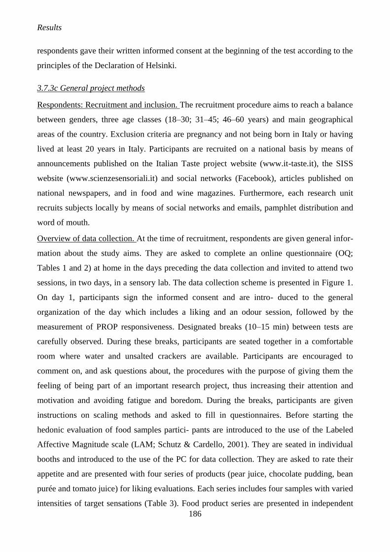
Results
186
respondents gave their written informed consent at the beginning of the test according to the
principles of the Declaration of Helsinki.
3.7.3c General project methods
Respondents: Recruitment and inclusion. The recruitment procedure aims to reach a balance
between genders, three age classes (18–30; 31–45; 46–60 years) and main geographical
areas of the country. Exclusion criteria are pregnancy and not being born in Italy or having
lived at least 20 years in Italy. Participants are recruited on a national basis by means of
announcements published on the Italian Taste project website (www.it-taste.it), the SISS
website (www.scienzesensoriali.it) and social networks (Facebook), articles published on
national newspapers, and in food and wine magazines. Furthermore, each research unit
recruits subjects locally by means of social networks and emails, pamphlet distribution and
word of mouth.
Overview of data collection. At the time of recruitment, respondents are given general infor-
mation about the study aims. They are asked to complete an online questionnaire (OQ;
Tables 1 and 2) at home in the days preceding the data collection and invited to attend two
sessions, in two days, in a sensory lab. The data collection scheme is presented in Figure 1.
On day 1, participants sign the informed consent and are intro- duced to the general
organization of the day which includes a liking and an odour session, followed by the
measurement of PROP responsiveness. Designated breaks (10–15 min) between tests are
carefully observed. During these breaks, participants are seated together in a comfortable
room where water and unsalted crackers are available. Participants are encouraged to
comment on, and ask questions about, the procedures with the purpose of giving them the
feeling of being part of an important research project, thus increasing their attention and
motivation and avoiding fatigue and boredom. During the breaks, participants are given
instructions on scaling methods and asked to fill in questionnaires. Before starting the
hedonic evaluation of food samples partici- pants are introduced to the use of the Labeled
Affective Magnitude scale (LAM; Schutz & Cardello, 2001). They are seated in individual
booths and introduced to the use of the PC for data collection. They are asked to rate their
appetite and are presented with four series of products (pear juice, chocolate pudding, bean
purée and tomato juice) for liking evaluations. Each series includes four samples with varied
intensities of target sensations (Table 3). Food product series are presented in independent
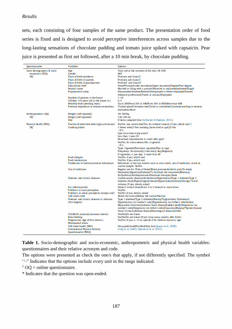
Results
187
sets, each consisting of four samples of the same product. The presentation order of food
series is fixed and is designed to avoid perceptive interferences across samples due to the
long-lasting sensations of chocolate pudding and tomato juice spiked with capsaicin. Pear
juice is presented as first set followed, after a 10 min break, by chocolate pudding.
Table 1. Socio-demographic and socio-economic, anthropometric and physical health variables:
questionnaires and their relative acronym and code.
The options were presented as check the one/s that apply, if not differently specified. The symbol
‘‘-” Indicates that the options include every unit in the range indicated. 1 OQ = online questionnaire.
* Indicates that the question was open-ended.
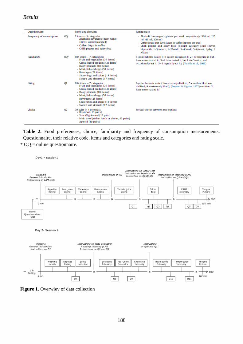
Results
188
Table 2. Food preferences, choice, familiarity and frequency of consumption measurements:
Questionnaire, their relative code, items and categories and rating scale.
* OQ = online questionnaire.
Figure 1. Overwiev of data collection
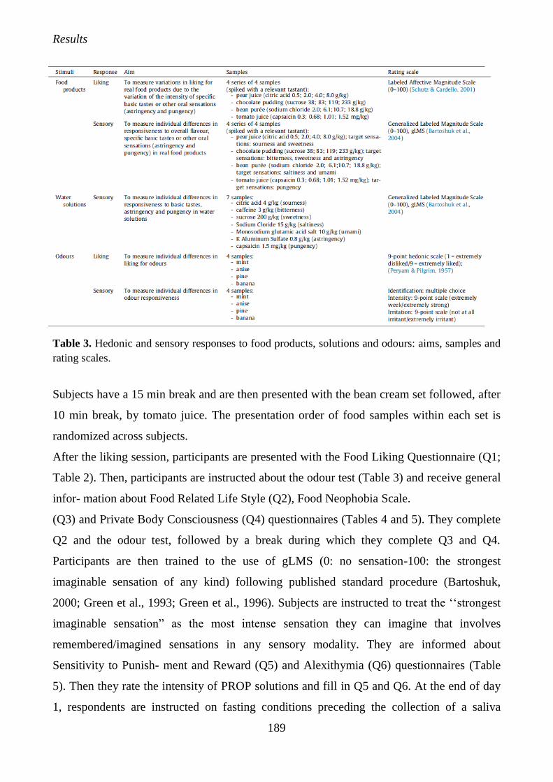
Results
189
Table 3. Hedonic and sensory responses to food products, solutions and odours: aims, samples and
rating scales.
Subjects have a 15 min break and are then presented with the bean cream set followed, after
10 min break, by tomato juice. The presentation order of food samples within each set is
randomized across subjects.
After the liking session, participants are presented with the Food Liking Questionnaire (Q1;
Table 2). Then, participants are instructed about the odour test (Table 3) and receive general
infor- mation about Food Related Life Style (Q2), Food Neophobia Scale.
(Q3) and Private Body Consciousness (Q4) questionnaires (Tables 4 and 5). They complete
Q2 and the odour test, followed by a break during which they complete Q3 and Q4.
Participants are then trained to the use of gLMS (0: no sensation-100: the strongest
imaginable sensation of any kind) following published standard procedure (Bartoshuk,
2000; Green et al., 1993; Green et al., 1996). Subjects are instructed to treat the ‘‘strongest
imaginable sensation” as the most intense sensation they can imagine that involves
remembered/imagined sensations in any sensory modality. They are informed about
Sensitivity to Punish- ment and Reward (Q5) and Alexithymia (Q6) questionnaires (Table
5). Then they rate the intensity of PROP solutions and fill in Q5 and Q6. At the end of day
1, respondents are instructed on fasting conditions preceding the collection of a saliva
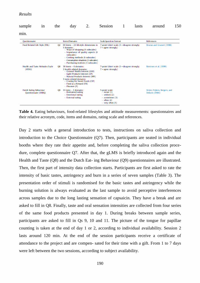
Results
190
sample in the day 2. Session 1 lasts around 150
min.
Table 4. Eating behaviours, food-related lifestyles and attitude measurements: questionnaires and
their relative acronym, code, items and domains, rating scale and references.
Day 2 starts with a general introduction to tests, instructions on saliva collection and
introduction to the Choice Questionnaire (Q7). Then, participants are seated in individual
booths where they rate their appetite and, before completing the saliva collection proce-
dure, complete questionnaire Q7. After that, the gLMS is briefly introduced again and the
Health and Taste (Q8) and the Dutch Eat- ing Behaviour (Q9) questionnaires are illustrated.
Then, the first part of intensity data collection starts. Participants are first asked to rate the
intensity of basic tastes, astringency and burn in a series of seven samples (Table 3). The
presentation order of stimuli is randomised for the basic tastes and astringency while the
burning solution is always evaluated as the last sample to avoid perceptive interferences
across samples due to the long lasting sensation of capsaicin. They have a break and are
asked to fill in Q8. Finally, taste and oral sensation intensities are collected from four series
of the same food products presented in day 1. During breaks between sample series,
participants are asked to fill in Qs 9, 10 and 11. The picture of the tongue for papillae
counting is taken at the end of day 1 or 2, according to individual availability. Session 2
lasts around 120 min. At the end of the session participants receive a certificate of
attendance to the project and are compen- sated for their time with a gift. From 1 to 7 days
were left between the two sessions, according to subject availability.
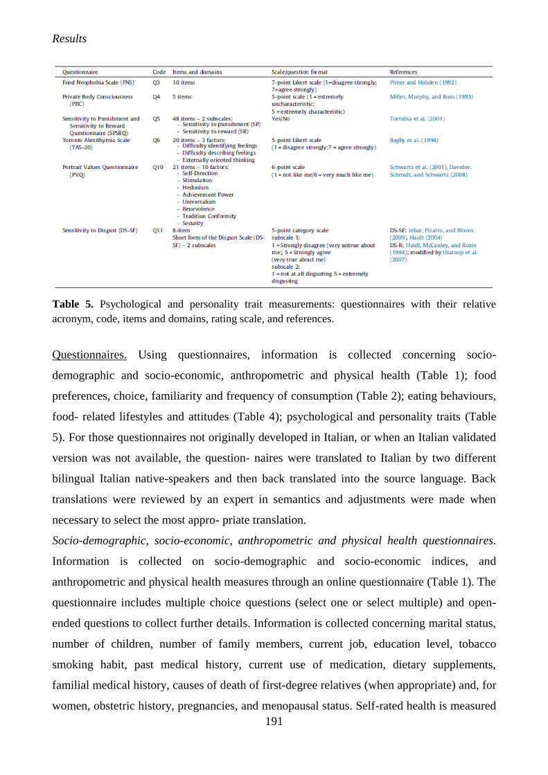
Results
191
Table 5. Psychological and personality trait measurements: questionnaires with their relative
acronym, code, items and domains, rating scale, and references.
Questionnaires. Using questionnaires, information is collected concerning socio-
demographic and socio-economic, anthropometric and physical health (Table 1); food
preferences, choice, familiarity and frequency of consumption (Table 2); eating behaviours,
food- related lifestyles and attitudes (Table 4); psychological and personality traits (Table
5). For those questionnaires not originally developed in Italian, or when an Italian validated
version was not available, the question- naires were translated to Italian by two different
bilingual Italian native-speakers and then back translated into the source language. Back
translations were reviewed by an expert in semantics and adjustments were made when
necessary to select the most appro- priate translation.
Socio-demographic, socio-economic, anthropometric and physical health questionnaires.
Information is collected on socio-demographic and socio-economic indices, and
anthropometric and physical health measures through an online questionnaire (Table 1). The
questionnaire includes multiple choice questions (select one or select multiple) and open-
ended questions to collect further details. Information is collected concerning marital status,
number of children, number of family members, current job, education level, tobacco
smoking habit, past medical history, current use of medication, dietary supplements,
familial medical history, causes of death of first-degree relatives (when appropriate) and, for
women, obstetric history, pregnancies, and menopausal status. Self-rated health is measured
Results
192
using the European World Health Organization (WHO) version (Jürges et al., 2008).
Anthropometric includes questions on height and weight and dietary restraint. To determine
eating habits, respondents are asked to indicate which diet they follow out of list of nine
eating diets descriptions adapted from De Backer and Hudders (2015). Information about
physical and sedentary activity is collected using the Italian version of the International
Physical Activity Questionnaire (IPAQ) (Craig et al., 2003; Mannocci et al., 2012). Physical
activity is described according to 3 levels of exercise intensity (walking, moderate or
vigorous), frequency of exercising (days/week) and daily duration of each performed
activity.
Food Familiarity, liking and choice questionnaires. Information about frequency of
consumption is collected for alcoholic bev- erages (beer; wine; spirits; aperitif/cocktail),
coffee, sugar addition in coffee and chilli pepper and spicy food (Table 2). The Food
Familiarity and Food Liking questionnaires were developed to measure, respectively,
familiarity with, and liking for, a selection of 184 foods appropriate in different eating
situations (Table 2). Eating situations were identified considering either the traditional
Italian meal pattern (breakfast, lunch and dinner), as well as new habits, such as snack/light
meals and aperitif, that tend to substitute lunch or dinner, thus breaking the traditional meal
timing. The item selection reflected variations in familiarity (more/less familiar foods),
flavour (strong/mild) and energy con- tent (high-energy/low-energy dense) as well. Items
are grouped in product categories based on their chemical composition. The presentation
order of the items within each product category as well as the product category order are
randomized across participants. The Food Choice Questionnaire was developed in order to
eval- uate preferences within a pair of items. For each pair, respondents are asked to indicate
which food they would choose in that specific eating situation. In this questionnaire, food
items (selected among the 184 items of the Food Familiarity and Liking questionnaires)
were grouped in 79 pairs and distributed in specific eating situa- tions as follows: breakfast
(13 pairs), snack/light-meal (13 pairs), main meal (either lunch or dinner, 43 pairs) and
aperitif (10 pairs). Items in each pair represent variations in terms of familiarity, taste (e.g.
bitter vs sweet) and energy content (e.g. low-fat vs full-fat). In some cases, pairs consist of
different foods or food categories (e.g. fruit vs cake) both suitable for a specific eating
situation (e.g. breakfast). The presentation order of the food items within each pair, and of
Results
193
the pairs within each eating context, is randomized across participants, while the
presentation order of the eating sit- uations is the same for all participants (breakfast,
snack/light-meal, main meal, aperitif).
Eating behaviours, food-related lifestyles and attitudes. Questionnaires are completed
during the course of the testing days to assess eating behaviours and attitudes towards foods.
Food-related lifestyles are determined using the Food Related Lifestyle (FRL)
questionnaire, while consumers’ orientations towards health and hedonic characteristics of
foods is determined through the Health and Taste Attitudes Scale (HTAS). The Dutch
Eating Beha- viour Questionnaire (DEBQ) is used to assess restrained, emotional and
external eating behaviours (Table 4).
Psychological and personality traits. Questionnaires are completed during the course of the
testing days to assess seven psychological or personality related traits: food neophobia
(FNS); private body consciousness (PBC), that it, awareness of internal sensations;
sensitivity to punishment and reward (SPSRQ); sensitivity to core disgust (DS-SF);
alexithymia (TAS-20); and orientation to value (PVQ); (Table 5).
Sensory stimuli. Water solutions. Seven water solutions, corresponding to five basic tastes,
astringent and burning sensations are rated for intensity (Table 3). The concentration of the
tastants were decided based on published psychophysical data (Feeney et al., 2014; Hayes et
al., 2010; Masi et al., 2015) and previous preliminary trials conducted with one-hundred
untrained subjects recruited in five Italian sensory laboratories (unpublished data) in order
to select solutions equivalent to moderate/strong on a gLMS. The results of the preliminary
trials were confirmed in a pilot study performed in 10 sensory laboratories with an average
number of 5 subjects per lab.
Food products. The criteria followed for the selection of foods for the study were: i) being
food or drink products widely consumed and distributed in Italy; ii) being simple and repro-
ducible to prepare (e.g. preferable ready-made products), to handle (e.g. to be consumed at
room temperature) and homogeneous in composition and aspect to be easily portioned (e.g.
liquids or semi solid). A pear juice (PJ), a chocolate pudding (CP), a bean purée (BP) and a
tomato juice (TJ) were selected as the most appropriate food matrices for testing the
responses to target tastes. For each food product, four levels of tastant concentration were
Results
194
selected to elicit a variation in the strength of target sensations (the five basic tastes and two
chemestetic sensations- astringency and pungency from weak to strong, Table 3). As with
the water solutions, the choice of concentration of tastants for each product was based on
published psychophysical data, preliminary tests (unpublished data) and the pilot study.
Odours. The odours were selected from the ones included in the European Test of Olfactory
Capabilities (Joussain et al., 2016) and presented using cardstocks designed for the project
‘‘La Préva- lence des troubles Olfactifs en France” (Projet DEFISENS – PREVAL– OLF)
coordinated by Moustafa Bensafi (CRNL, Lyon, France) who kindly provided the material.
Odorant molecules were trapped in tight microcapsules (aminoplast type, diameter: 4–8
micro). The microcapsule-based ink was printed on a cardstock (SILK-250 g; Dimension:
11 cm x 21 cm). Each odorant was printed on a delimited area (2 cm2 disc). The release of
the odour is done simply by rubbing the printed microcapsule reserve. Liking, intensity,
identification and irritation are measured for each odour: mint, anise, pine, banana. First, the
odorant is pre- sented and the respondent is asked to identify the name of the odour among
four possibilities. Then, the respondent is asked to evaluate the odour’s intensity, its degree
of irritation, and how much they like it. The odorants are presented in a randomized order
and a break of one minute is observed between each evaluation.
Taste function indices. Fungiform papillae number. The anterior portion of the dor- sal
surface of the tongue is swabbed with household blue food col- oring, using a cotton-tipped
applicator. This made the FP easily visible as red structures against the blue background of
the stained tongue. Digital pictures of the tongue are recorded (Shahbake et al., 2005) using
a digital microscope (MicroCapture, version 2.0 for 20×-400×) (Masi et al., 2015). For each
participant, the clearest image is selected, and the number of FP is counted in two 0.6 cm
diameter circles, one on right side and one on left side of tongue, 0.5 cm from the tip and
0.5 cm from the tongue midline. The number of FP is manually counted by two researchers
independently according to Denver Papillae Protocol (Nuessle et al., 2015). The average of
these values is used for each subject.
PROP taster status. A 3.2 mM PROP solution is prepared by dissolving 0.5447 g/L of 6-n-
propyl-2-thiouracil (European Phar- macopoeia Reference Standard, Sigma Aldrich,
Milano, IT) into deionized water (Prescott et al., 2004). Subjects are presented with 2
Results
195
identical samples (10 ml) coded with a three-digit code. Subjects are instructed to hold each
sample (10 ml) in their mouth for 10 s, then expectorate, wait 20s and evaluate the intensity
of bitterness using the gLMS (Bartoshuk et al., 2004). Subjects have a 90s break in order to
control for carry-over effect after the first sample evaluation. During the break, subjects
rinse their mouths with distilled water for 30 s, have some plain crackers for 30 s, and
finally rinse their mouths with water for a further 30s. The average bitterness score is used
for each subject.
Genotyping. Saliva samples are collected from all participants using the Norgen Saliva
DNA collection and preservation devices. DNA extraction is then performed using the
Saliva DNA Isolation kit, according to the manufacturer’s instructions (Norgen Biotek
Corp; Ontario, Canada). Genotyping of these samples is carried out using Illumina
MEGAEX high-density SNP chip array (Illumina, Inc., San Diego, CA, USA), which
contains > 2 millions of selected markers. After quality control, samples will be imputed
using the 1000G Project phase 3 reference (Auton et al., 2015) plus an INGI (Italian
Network of Genetic Isolates) reference panel, for a total of about 88.000.000 markers.
3.7.4 Preliminary project dataset and analysis of selected variables
One of the aims of the present paper is to show the potential of the IT dataset on the basis of
the results from the first year of the study, based on data from 1225 individuals. For this
purpose, we selected a limited number of variables from the complete set in the project. The
aim of reporting this particular set of data is to show how measurement of multiple variables
provides an advantage in understanding food preferences. The variables reported here are:
demographics (age and gender), biological (PROP status), psychological (food neophobia,
sensitivity to reward and punishment), socio-cultural (health and taste attitudes) and
behavioural (familiarity for specific vegetables). For these variables, we described the
distribution of the data and studied both gender and age effects. In addition, we investigated
the role of these variables in determining preferences (stated liking) for specific vegetables:
rocket and radish salads. We selected these items for the following reasons: 1)
understanding consumer liking for vegetables is relevant in itself because of the general
interest in promoting health eating in many countries (Appleton et al., 2016); 2) the sensory
properties of radish and rocket (bitterness and pungency) may represent a potential barrier
Results
196
to consumption (Dinnella et al., 2016). Liking for Brassica vegetables has been reported to
be affected by PROP status (Shen et al., 2016) and psychological traits (i.e. the level of
neophobia in adult subjects has been found to be a barrier to the development of preference
for vegetables in relation to their sensory properties; Törnwall et al., 2014). Thus, they are
appropriate to set up a multidimensional model to show the potential of the Italian Taste
dataset in studying the association among several different variables affecting food choice.
3.7.4a Matherials and methods
Participants. The data from 1225 participants were collected during 2015. Their
demographic and social characteristics are reported in Table 6. The sample was 61% female
with a mean age of 36.9 years (SD 12.8; 18–60 years old range). The age distributions of the
male and female groups were not significantly different. Regarding the region of residence
of the respondents, the Northern of Italy was the most represented (46%), followed by the
Southern and Islands (34%) and by the central area of Italy (20%) in line with ISTAT data
(ISTAT, 2011). As expected, more females were in the normal range and underweight than
males, whereas more males were overweight or obese (v2 = 15.8; p < 0.01). 14% percent of
the respondents smoked regularly and 11% occasionally. The vast majority of respondents
(more than 90%) reported no history of food allergy and/or intolerance. Vegetarians were
the 2.2% of the total. Almost all enrolled subjects attended the first laboratory session (more
than 99%). Around 3% of subjects dropped out after the first session, generally due to time
constraints.
Measuring sensitivity to PROP. PROP status was assessed according to the procedure
described above.
Personality and attitude measures. Food neophobia scale (FNS). The trait of food
neophobia, defined as the reluctance to try and eat unfamiliar foods, was quantified using
the 10-item instrument developed by Pliner and Hobden (1992). The individual FNS scores
were computed as the sum of ratings given to the ten statements, after the neophilic items
had been reversed; the scores thus ranged from 10 to 70, with higher scores reflecting higher
food neophobia levels.
Sensitivity to punishment and sensitivity to reward questionnaire (SPSRQ). According to
Gray’s neuropsychological theory of personality, two basic brain systems control behaviour
and emotions: the Behavioural Inhibition System (BIS) and the Behavioural Activation
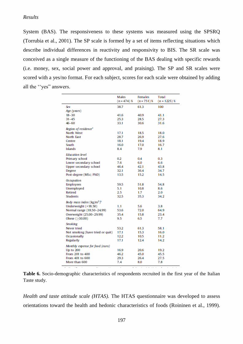
Results
197
System (BAS). The responsiveness to these systems was measured using the SPSRQ
(Torrubia et al., 2001). The SP scale is formed by a set of items reflecting situations which
describe individual differences in reactivity and responsivity to BIS. The SR scale was
conceived as a single measure of the functioning of the BAS dealing with specific rewards
(i.e. money, sex, social power and approval, and praising). The SP and SR scales were
scored with a yes/no format. For each subject, scores for each scale were obtained by adding
all the ‘‘yes” answers.
Table 6. Socio-demographic characteristics of respondents recruited in the first year of the Italian
Taste study.
Health and taste attitude scale (HTAS). The HTAS questionnaire was developed to assess
orientations toward the health and hedonic characteristics of foods (Roininen et al., 1999).
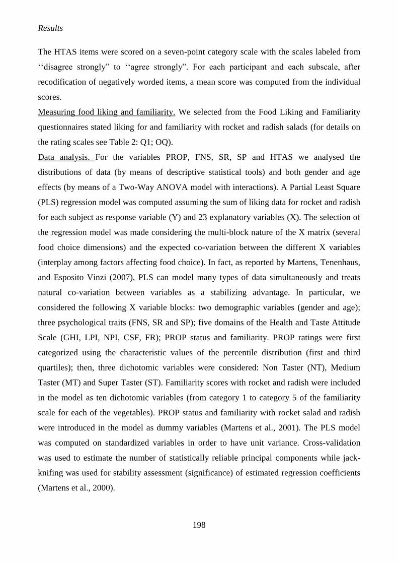
Results
198
The HTAS items were scored on a seven-point category scale with the scales labeled from
‘‘disagree strongly” to ‘‘agree strongly”. For each participant and each subscale, after
recodification of negatively worded items, a mean score was computed from the individual
scores.
Measuring food liking and familiarity. We selected from the Food Liking and Familiarity
questionnaires stated liking for and familiarity with rocket and radish salads (for details on
the rating scales see Table 2: Q1; OQ).
Data analysis. For the variables PROP, FNS, SR, SP and HTAS we analysed the
distributions of data (by means of descriptive statistical tools) and both gender and age
effects (by means of a Two-Way ANOVA model with interactions). A Partial Least Square
(PLS) regression model was computed assuming the sum of liking data for rocket and radish
for each subject as response variable (Y) and 23 explanatory variables (X). The selection of
the regression model was made considering the multi-block nature of the X matrix (several
food choice dimensions) and the expected co-variation between the different X variables
(interplay among factors affecting food choice). In fact, as reported by Martens, Tenenhaus,
and Esposito Vinzi (2007), PLS can model many types of data simultaneously and treats
natural co-variation between variables as a stabilizing advantage. In particular, we
considered the following X variable blocks: two demographic variables (gender and age);
three psychological traits (FNS, SR and SP); five domains of the Health and Taste Attitude
Scale (GHI, LPI, NPI, CSF, FR); PROP status and familiarity. PROP ratings were first
categorized using the characteristic values of the percentile distribution (first and third
quartiles); then, three dichotomic variables were considered: Non Taster (NT), Medium
Taster (MT) and Super Taster (ST). Familiarity scores with rocket and radish were included
in the model as ten dichotomic variables (from category 1 to category 5 of the familiarity
scale for each of the vegetables). PROP status and familiarity with rocket salad and radish
were introduced in the model as dummy variables (Martens et al., 2001). The PLS model
was computed on standardized variables in order to have unit variance. Cross-validation
was used to estimate the number of statistically reliable principal components while jack-
knifing was used for stability assessment (significance) of estimated regression coefficients
(Martens et al., 2000).
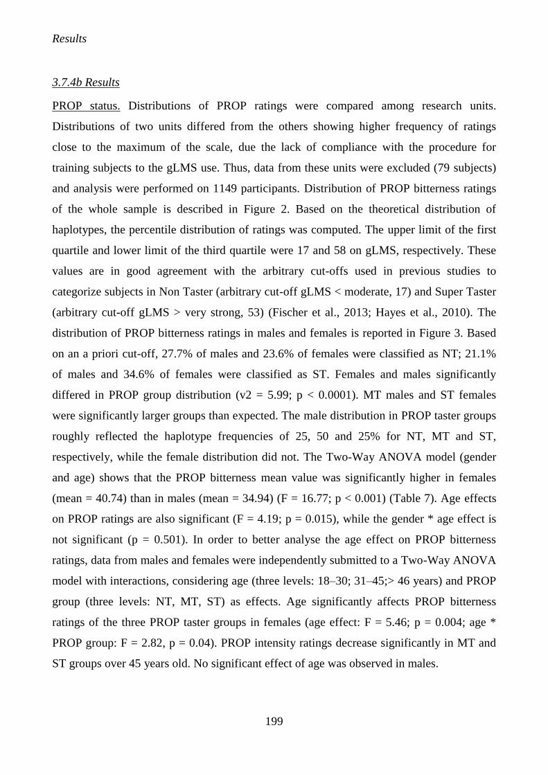
Results
199
3.7.4b Results
PROP status. Distributions of PROP ratings were compared among research units.
Distributions of two units differed from the others showing higher frequency of ratings
close to the maximum of the scale, due the lack of compliance with the procedure for
training subjects to the gLMS use. Thus, data from these units were excluded (79 subjects)
and analysis were performed on 1149 participants. Distribution of PROP bitterness ratings
of the whole sample is described in Figure 2. Based on the theoretical distribution of
haplotypes, the percentile distribution of ratings was computed. The upper limit of the first
quartile and lower limit of the third quartile were 17 and 58 on gLMS, respectively. These
values are in good agreement with the arbitrary cut-offs used in previous studies to
categorize subjects in Non Taster (arbitrary cut-off gLMS < moderate, 17) and Super Taster
(arbitrary cut-off gLMS > very strong, 53) (Fischer et al., 2013; Hayes et al., 2010). The
distribution of PROP bitterness ratings in males and females is reported in Figure 3. Based
on an a priori cut-off, 27.7% of males and 23.6% of females were classified as NT; 21.1%
of males and 34.6% of females were classified as ST. Females and males significantly
differed in PROP group distribution (v2 = 5.99; p < 0.0001). MT males and ST females
were significantly larger groups than expected. The male distribution in PROP taster groups
roughly reflected the haplotype frequencies of 25, 50 and 25% for NT, MT and ST,
respectively, while the female distribution did not. The Two-Way ANOVA model (gender
and age) shows that the PROP bitterness mean value was significantly higher in females
(mean = 40.74) than in males (mean = 34.94) (F = 16.77; p < 0.001) (Table 7). Age effects
on PROP ratings are also significant (F = 4.19; p = 0.015), while the gender * age effect is
not significant (p = 0.501). In order to better analyse the age effect on PROP bitterness
ratings, data from males and females were independently submitted to a Two-Way ANOVA
model with interactions, considering age (three levels: 18–30; 31–45;> 46 years) and PROP
group (three levels: NT, MT, ST) as effects. Age significantly affects PROP bitterness
ratings of the three PROP taster groups in females (age effect: F = 5.46; p = 0.004; age *
PROP group: F = 2.82, p = 0.04). PROP intensity ratings decrease significantly in MT and
ST groups over 45 years old. No significant effect of age was observed in males.
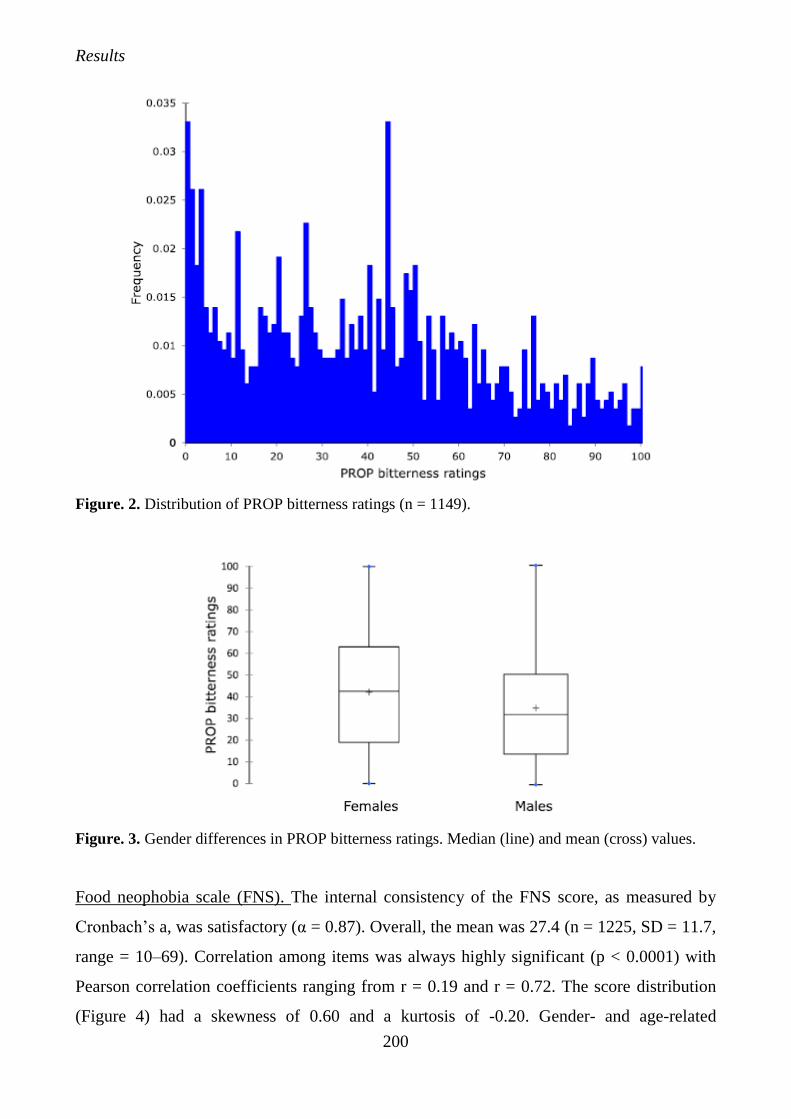
Results
200
Figure. 2. Distribution of PROP bitterness ratings (n = 1149).
Figure. 3. Gender differences in PROP bitterness ratings. Median (line) and mean (cross) values.
Food neophobia scale (FNS). The internal consistency of the FNS score, as measured by
Cronbach’s a, was satisfactory (α = 0.87). Overall, the mean was 27.4 (n = 1225, SD = 11.7,
range = 10–69). Correlation among items was always highly significant (p < 0.0001) with
Pearson correlation coefficients ranging from r = 0.19 and r = 0.72. The score distribution
(Figure 4) had a skewness of 0.60 and a kurtosis of -0.20. Gender- and age-related
Results
201
differences in FNS scores were tested through Two-way ANOVA with interaction (Table
7), which showed a significant main effect of gender (F = 4.24, p < 0.043) and age (F =
7.26, p < 0.001). Males (mean = 28.3) were significantly more neophobic than females
(mean = 26.9) and the youngest participants (18–30 years: mean = 25.9) were significantly
less neophobic than the older group (>46 years: mean = 28.9). FNS scores of the middle-
aged group (31–45 years: M = 27.9) lay in between. The age * gender interaction was not
significant.
Table 7. Two-Way ANOVA. Gender, age and their interaction effect on selected variables: mean
scores and p-values.
In bold significant values. Letters indicate significantly different mean scores (Tukey’s Honest
Significant Difference, HSD).
* The total degree of freedom (d.f.) for each of the computed ANOVA models was 1219 with
exception of the variable PROP (d.f. = 1143).
** HTAS domains.
Sensitivity to punishment (SP) and sensitivity to reward (SR). The Cronbach’s a for each of
the scales was good, this being slightly higher for the SP (0.84) than for SR (0.75) scale.
The two scales were poorly correlated with each other (r = 0.061, p = 0.035). We also
observed sufficient variation in scores: out of a possible range of 0–24, SP scores ranged
from 0 to 24 (mean = 10.01; SD = 5.26) while SR ranged from 0 to 22 (mean = 8.92; SD =
3.96). The Two-Way ANOVA model with interaction (Table 7) computed on the SP and SR
scores showed a significant effect of both gender and age, while the interaction effect was
not significant. Females obtained higher scores than males on the SP scale, while males
clearly score higher than females on the SR scales (p < 0.001). Both SP and SR scores in
participants aged 18–30 were higher than in participants > 31 years old. In addition, on the
SR scale, participants 31–45 obtained higher scores than subjects 46–60 (p < 0.001).
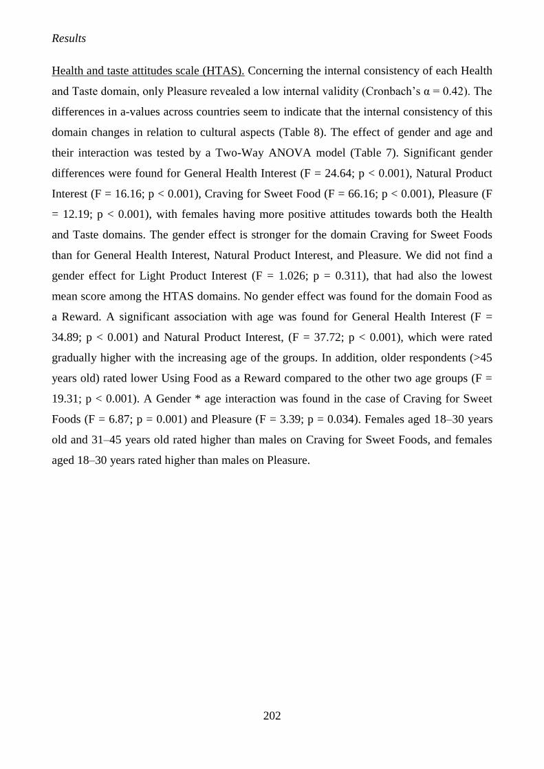
Results
202
Health and taste attitudes scale (HTAS). Concerning the internal consistency of each Health
and Taste domain, only Pleasure revealed a low internal validity (Cronbach’s α = 0.42). The
differences in a-values across countries seem to indicate that the internal consistency of this
domain changes in relation to cultural aspects (Table 8). The effect of gender and age and
their interaction was tested by a Two-Way ANOVA model (Table 7). Significant gender
differences were found for General Health Interest (F = 24.64; p < 0.001), Natural Product
Interest (F = 16.16; p < 0.001), Craving for Sweet Food (F = 66.16; p < 0.001), Pleasure (F
= 12.19; p < 0.001), with females having more positive attitudes towards both the Health
and Taste domains. The gender effect is stronger for the domain Craving for Sweet Foods
than for General Health Interest, Natural Product Interest, and Pleasure. We did not find a
gender effect for Light Product Interest (F = 1.026; p = 0.311), that had also the lowest
mean score among the HTAS domains. No gender effect was found for the domain Food as
a Reward. A significant association with age was found for General Health Interest (F =
34.89; p < 0.001) and Natural Product Interest, (F = 37.72; p < 0.001), which were rated
gradually higher with the increasing age of the groups. In addition, older respondents (>45
years old) rated lower Using Food as a Reward compared to the other two age groups (F =
19.31; p < 0.001). A Gender * age interaction was found in the case of Craving for Sweet
Foods (F = 6.87; p = 0.001) and Pleasure (F = 3.39; p = 0.034). Females aged 18–30 years
old and 31–45 years old rated higher than males on Craving for Sweet Foods, and females
aged 18–30 years rated higher than males on Pleasure.
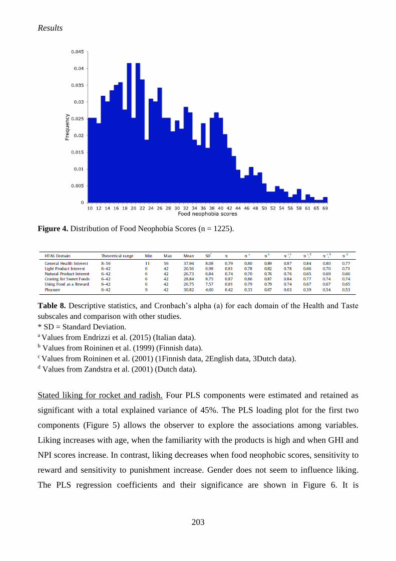
Results
203
Figure 4. Distribution of Food Neophobia Scores (n = 1225).
Table 8. Descriptive statistics, and Cronbach’s alpha (a) for each domain of the Health and Taste
subscales and comparison with other studies.
* SD = Standard Deviation. a Values from Endrizzi et al. (2015) (Italian data). b Values from Roininen et al. (1999) (Finnish data). c Values from Roininen et al. (2001) (1Finnish data, 2English data, 3Dutch data). d Values from Zandstra et al. (2001) (Dutch data).
Stated liking for rocket and radish. Four PLS components were estimated and retained as
significant with a total explained variance of 45%. The PLS loading plot for the first two
components (Figure 5) allows the observer to explore the associations among variables.
Liking increases with age, when the familiarity with the products is high and when GHI and
NPI scores increase. In contrast, liking decreases when food neophobic scores, sensitivity to
reward and sensitivity to punishment increase. Gender does not seem to influence liking.
The PLS regression coefficients and their significance are shown in Figure 6. It is
Results
204
interesting to note that being a PROP ST is, as expected, negatively associated with liking
and positively associated with a low familiarity with the two vegetables.
3.7.4c Discussion
We applied a PLS model to study the associations among a selected number of variables in
affecting stated liking for two vegetables. The purpose of the analysis was to give an
example of how to explore and understand the complex picture determined by the interplay
of biological, physiological, psychological and sociocultural factors determining individual
differences in food preferences and choice, very well depicted by several authors already
cited in the introduction of this paper. Our relatively simple example clearly showed that
individual differences in stated liking for two specific vegetables characterized by sensory
properties such as bitterness and pungency are driven by experience and exposure.
However, some psychological traits, such as being neophobic or sensible to reward and to
punishment may act as barriers to this process. The importance of food neophobia among a
variety of variables in modulating flavour preferences in young adult subjects (21–25 y.o.)
has been highlighted by Törnwall et al. (2014). In addition, our findings indicate that
psychological traits potentially involved in explaining individual food choices are not
limited to food neophobia. Our results suggest that sensitivity to reward and punishment
could also play a relevant role as barriers to exposure and familiarization with specific
foods. In fact, both higher SP and SR were associated with a lower liking for radish and
rocket salad, thus representing a possible barrier to vegetable consumption. Recent studies
have highlighted an association between these traits and unhealthier behaviours; higher
sensitivity to reward predicted higher fat intake, higher alcohol consumption, greater
likelihood of binge drinking, greater likelihood of being a smoker and, amongst smokers,
smoking frequency. Higher sensitivity to punishment predicted lower alcohol consumption
but higher sugar intake (Tapper et al., 2015). Higher SR scores were significantly related
with a more frequent drinking and heavier consumption per occasion of alcohol. In addition,
drinkers more sensitive to reward reported feeling more stimulated shortly after drinking
and exhibited an attenuated rate of decline in stimulation over the blood alcohol curve,
relative to drinkers with less strong reward sensitivity (Morris et al., 2016). The Italian
Taste dataset represents an opportunity to study more in depth the contribution of these
Results
205
traits to unhealthy food behaviours investigating their association to preferences for specific
food categories such as vegetables. This may be particularly worth of investigation in the
case of younger adults, that we found more sensitive both to reward and punishment: for
this age group these traits can play a role in creating a barrier to consumption of healthier
products or encouraging unhealthier food behaviours. Finally, the model suggests that being
a ST phenotype may also mediate familiarity with and thus liking for specific food, as
reported by Prescott and co-workers (Lee et al., 2008; Yeomans et al., 2009). In this
example, there is good evidence for the interplay between factors affecting liking: some
psychological traits like food neophobia, sensitivity to reward and punishment and
phenotype characteristics (PROP taste group) represent possible barriers to consumption of
the considered vegetables because of their negative effect on liking. In contrast, age and
experience, interpreted as familiarity with the products and acquired attitudes (GHI, NPI),
facilitated liking and thus consumption. Considering the PLS model as an example and
interpreting its results in a broader view, we suggest that coupling the measurement of many
variables related to food preferences with appropriate multidimensional statistical analysis
allows the researcher to obtain relevant information to answer to either applied or more
fundamental research questions. In fact, it is possible to identify variables that are relevant
for consumer segmentation in relation to the acceptance of specific products. At same time,
the obtained information is relevant even when the research question is how to overcome
barriers to the consumption of specific healthy foods in respect to segments clearly
characterized for their physiological, psychological, and socio-cultural traits. Overall, the
project sample to date has been quite well balanced in terms of gender, age (within the
range 18–60 years) and geographic areas. The proportion between the two sexes among
respondents is in line with other large scale studies (e.g. Pirastu et al., 2016) and can be
judged acceptable, considering that males tend to be less inclined to volunteer for research
than females, as clearly shown also in the NutriNet Santé study (Hercberg et al., 2010;
Méjean et al., 2014). The analysis of the structure and distribution of the data for each of the
selected variables allowed us to draw several conclusions regarding the variables presented
here.
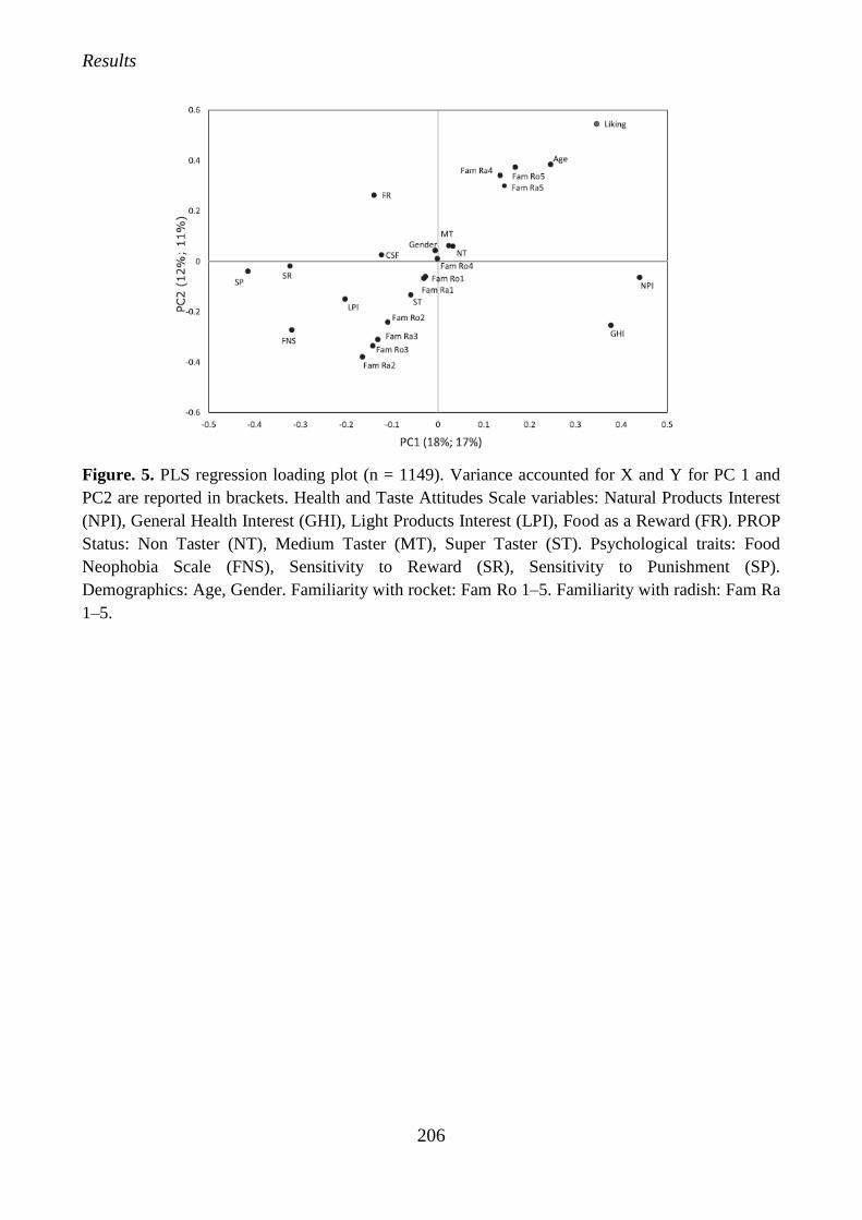
Results
206
Figure. 5. PLS regression loading plot (n = 1149). Variance accounted for X and Y for PC 1 and
PC2 are reported in brackets. Health and Taste Attitudes Scale variables: Natural Products Interest
(NPI), General Health Interest (GHI), Light Products Interest (LPI), Food as a Reward (FR). PROP
Status: Non Taster (NT), Medium Taster (MT), Super Taster (ST). Psychological traits: Food
Neophobia Scale (FNS), Sensitivity to Reward (SR), Sensitivity to Punishment (SP).
Demographics: Age, Gender. Familiarity with rocket: Fam Ro 1–5. Familiarity with radish: Fam Ra
1–5.
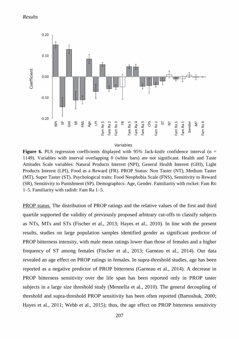
Results
207
Figure 6. PLS regression coefficients displayed with 95% Jack-knife confidence interval (n =
1149). Variables with interval overlapping 0 (white bars) are not significant. Health and Taste
Attitudes Scale variables: Natural Products Interest (NPI), General Health Interest (GHI), Light
Products Interest (LPI), Food as a Reward (FR). PROP Status: Non Taster (NT), Medium Taster
(MT), Super Taster (ST). Psychological traits: Food Neophobia Scale (FNS), Sensitivity to Reward
(SR), Sensitivity to Punishment (SP). Demographics: Age, Gender. Familiarity with rocket: Fam Ro
1–5. Familiarity with radish: Fam Ra 1–5.
PROP status. The distribution of PROP ratings and the relative values of the first and third
quartile supported the validity of previously proposed arbitrary cut-offs to classify subjects
as NTs, MTs and STs (Fischer et al., 2013; Hayes et al., 2010). In line with the present
results, studies on large population samples identified gender as significant predictor of
PROP bitterness intensity, with male mean ratings lower than those of females and a higher
frequency of ST among females (Fischer et al., 2013; Garneau et al., 2014). Our data
revealed an age effect on PROP ratings in females. In supra-threshold studies, age has been
reported as a negative predictor of PROP bitterness (Garneau et al., 2014). A decrease in
PROP bitterness sensitivity over the life span has been reported only in PROP taster
subjects in a large size threshold study (Mennella et al., 2010). The general decoupling of
threshold and supra-threshold PROP sensitivity has been often reported (Bartoshuk, 2000;
Hayes et al., 2011; Webb et al., 2015); thus, the age effect on PROP bitterness sensitivity
Results
208
deserves further investigation. PROP status classification based on phenotype might also
reflect the oral responsiveness due to other factors, such as fungiform papillae density,
which in turn are affected by age. The interplay between responsiveness to PROP bitterness
and fungiform papillae density has been reported in taster subjects depending on their
genotype (Hayes et al., 2008). The relationships between genotype and phenotype, as well
as responsiveness to PROP and fungiform papillae density, deserve further investigation and
will be explored as part of the Italian Taste project as soon as population genotyping is
completed.
Food neophobia. Since research on food neophobia suffers from a lack of standardization in
the age groups being compared, and in the number of participants involved (Meiselman et
al., 2010), the present results will be discussed only considering previous nationally
representative samples of consumers with a similar age range as the one considered in our
study. The analysis conducted on Food Neophobia scores showed that the internal validity
(a) of data was similar to that reported in other large studies, confirming that FNS is a robust
and efficient tool even when translated in other languages (Ritchey et al., 2003). In fact,
internal consistency of the FNS scores in the present study (a = 0.87, n = 1225, age range =
18–66 years) was similar to those reported in previous research involving large population
samples of Finns (a = 0.88, n = 2191, age range = 18–57 years, Knaapila et al., 2015; a =
0.85, n = 1083, age range = 16–80 years, Tuorila et al., 2001) and Swiss (a = 0.80, n = 4436,
age range: 21–99 years, Siegrist et al., 2013). The mean FNS score observed here (27.4, SD
= 11.7) was considerably lower than the one reported in a study performed in a sample of
Italian subjects of similar age (mean = 34.0, SD = 15.5, n = 167, age range = 20–59 years,
Demattè et al., 2013) and moderately lower than the mean FNS score found for Finns (mean
= 28.5, SD = 11.0, N = 2191, age range = 18–57 years, Knaapila et al., 2015). Cultural
origins may explain the difference between our results and those by Knaapila et al. (2015)
but not the difference with the outcome of Demattè et al. (2013). In this latter case, it might
be hypothesized that the sample was small, local and not representative of the general
Italian population. However, considering that in Italy strong regional differences in food
culture exist, the Italian Taste dataset has the potential to explore the differences among
geographic macro-areas of the country (North, Central and South) that also reflect socio-
economical differences. Significant effects of age and gender on FNS were found. We
Results
209
found a significant, though somewhat modest, effect of gender on FNS score, with males
being more neophobic than females. Analysis of nationally representative studies involving
consumers of comparable age to the one considered in the present study showed no gender
effect in one study (Knaapila et al., 2015) or a slight effect in three other studies (Hursti et
al., 1997; Siegrist et al., 2013; Tuorila et al., 2001). When gender-related differences were
found, all studies agreed that males were more neophobic than females. This has been
explained by the greater involvement of women rather than men in food purchase and
preparation (Hursti et al., 1997). However, it should be pointed out that the effect of gender
on FNS scores was always very small (from 1.5 to 2.9 points on a scale ranged from 10 to
70), leading to the conclusion that such effects are likely to be less important than many
other variables related to food rejection (Nordin et al., 2004). Similarly, the effect of age,
although significant, was somewhat weak. However, FNS scores tend to increase with age.
Age-related differences in the level of food neophobia are often reported in large population
studies, with FNS scores increasing with age (Meiselman et al., 2010; Siegrist et al., 2013;
Tuorila et al., 2001). Further analysis of the current dataset may reveal age and gender
effects on specific FNS items. At same time, the Italian Taste dataset will facilitate the study
of the associations between this trait and other psychological and biological measurements,
as well as with attitudes relevant to food choice.
Sensitivity to reward and sensitivity to punishment. In line with previous results (O’Connor
et al., 2004; Torrubia et al., 2001), the internal validity (a) of both scales was good, being
slightly higher for the SP than for SR scale. Our results confirm that the two personality
traits seem to be uncorrelated. The gender effect was in line with previous results (Caseras
et al., 2003; Torrubia et al., 2001), with females more sensitive to punishment than males,
and males more sensitive to reward than females. To our knowledge, the age effect on
sensitivity to reward and sensitivity to punishment scores in adult populations (e.g. from 18
to 60 years old) has not been studied in depth yet. In a study that used the BIS/BAS scale
developed by Carver and White (1994), Pagliaccio et al. (2016) observed that both
sensitivity to reward and punishment scores tended to be higher in young adulthood (18–22
years old) than in later adulthood (30–45 years old) and in childhood. Our data clearly show
that both sensitivity to reward and sensitivity to punishment are higher in the younger adults
Results
210
aged 18–30, and that individuals aged 31–45 tend to be more sensitive to reward than older
individuals.
Health and Taste attitudes. It has been shown that the HTAS predicts choices between
products varying in health and hedonic aspects and it has been consequently used to
segment consumers (Tuorila, 2015). In the present study, the internal validity (a) of the sub-
scales is generally in line with other studies for five out of six domains. The Cronbach’s a
value is not satisfactory for the Pleasure domain only. It seems that when this domain is
used in countries different from the one in which the questionnaire was developed, the
scores for each of the statements tend to be not strongly related each other. The
interpretation of the meaning of the statements describing the link of food with pleasure
could vary from culture to culture (Rozin et al., 1999), thus a translation-back translation
could not always be sufficient to guarantee the adherence with the original meaning. Further
studies on the adaptation of this domain taking into account the relevant socio-cultural
aspects of the country in which the study is conducted are needed. Roininen et al. (1999,
2001) registered comparable mean scores in the three domains of the Health subscale,
although with some differences between countries (2001). We noticed a low interest of the
Italian sample for light products which reflects a general tendency in the country to consider
the Mediterranean diet healthy and tasty at same time (Monteleone et al., 2009), with a
consequent low interest in light foods. Early studies from the HTAS questionnaire creators
pointed out a noticeable variability in values among gender, age and countries and their
interactions (Roininen et al., 1999, 2001). Our results partially confirm previous findings,
with females having more positive attitudes towards both the Health and Taste domains
(Endrizzi et al., 2015; Roininen et al., 1999, 2001). However, we found a stronger gender
effect for the domain Craving for Sweet Foods than for General Health Interest, Natural
Product Interest, and Pleasure, while in the previous studies reported above, a strongest
effect of gender for the General Health Interest domain was reported. The variability
induced by the gender by age interaction on HTAS scores deserves further investigations as
well as the effectiveness of this set of scales of predicting choices, even in association with
other variables.
Results
211
3.7.5 Conclusions
Studies on influences on food choice are subjected to two main limitations: the sample size
and an approach based on a limited perspective that does not take into account at the same
time genetics, taste sensitivity, psychographics and sensory and hedonic responses to foods
based on evaluations of samples and not only of names or tastant in solution. The Italian
Taste project plans to overcome the above-mentioned limitations and may be seen as a
model to explore the complex interplay of factors contributing to food choices. The design
of the study we presented here may in fact easily be reproduced in other countries, with the
precaution of adapting the Food Liking and Choice questionnaires taking into account the
specificities of the food culture considered and selecting appropriately the products used for
the sensory and hedonic tests among commonly consumed products. The exploration of
cross-cultural differences will contribute to a further deeper insight into the understanding
of food choices. In recent years, multicenter research has become increasingly common in
situations in which single research centres have the tools and skills to investigate a question,
but the power of data would suffer due to slow data collection or too few available
respondents. The present report describes a project in which Italian researchers have rallied
their resources to investigate human food choice behaviour and preferences using current
knowledge of possible predictors from genetic, physiological and psycho-social domains.
When planning a multicentre research, it is particularly important to ensure the alignment in
the procedure of data collection of the different labs involved in the study. Specific attention
should be paid to the procedure of sample preparation, papilla count and to the instructions
on the use of the gLMS. Training periods of all the researchers involved in data collection
are recommended to guarantee the reduction of differences due to the operators. Great
attention is also required to align the instructions to give to the respondents before and
during the test, in order to avoid an effect of different type of information given.
3.7.6 Acknowledgements
On behalf of the Italian Sensory Science Society the authors would like to thank all the
individuals who participated in the Italian Taste study and all the SISS members and their
institutions for their contribution to the project. The Italian Taste project is funded by the
Results
212
Italian Sensory Science Society and was partly supported in 2015 by the Louis Bonduelle
Foundation.
3.7.7 Appendix 1
A scientific committee of thirteen members of the Italian Sensory Science Society (SISS),
all experienced and internationally recognized researchers, designed the study. Each
member of the scientific committee coordinated one of the following activities: ethics,
bibliography, recruitment; liking/choice/familiarity questionnaires; attitudes and
psychological traits; liking and sensory tests; genetic tests; data analysis; database
implementation and management; communication; fund raising. The corresponding author
of the present paper served as project coordinator. Working groups open to all SISS
members were organized to define a procedure for each activity under the responsibility of a
coordinator. All the procedures related to data collection and data analysis were reviewed by
the members of an international advisory board composed by experienced sensory and
consumer researchers. Procedures were revised according to their advice and tested in pilot
studies before the approval of the scientific committee. Similarly, a general procedure for
data acquisition was designed, reviewed, and tested in a pilot study run in April-June 2015
with 95 respondents (5 in each of the 19 laboratories involved in the project, (Table 9).
During the pilot study a checklist was provided to each unit to report deviations from the
procedures. The checklist included the control of the following critical points: sample
preparation (time between preparation of food sample and testing; time between the two
sessions; temperature of conservation of samples); papilla count (two-way ANOVA to
investigate the effect of the operators, if any), critical points for each step of the test;
missing data; data control. After a final revision, the data acquisition procedure was
approved by the scientific committee and data collection started in July 2015 with the
objective of recruiting three thousand respondents in three years across the laboratories and
the country. Sixteen labs out of nineteen utilized the same computerised system for data
collection in the lab (Fizz, Biosystèmes, France). Methods were centrally designed at
Florence University. Four units collected data on paper forms prepared on the basis of the
Fizz sessions. Before the pilot studies, two days of training were organised at the Sensory
Lab of Florence University in order to uniform the PROP and papillae procedures. Special
attention was paid to training researchers from all the labs in the use of the gLMS.
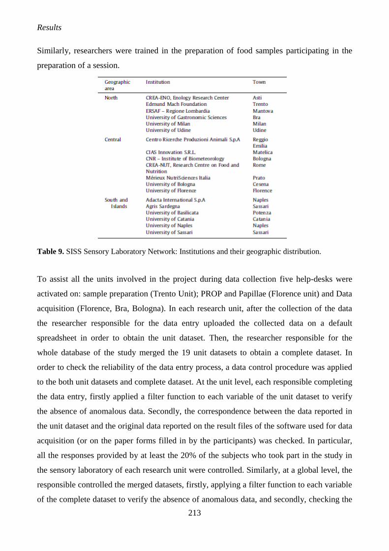
Results
213
Similarly, researchers were trained in the preparation of food samples participating in the
preparation of a session.
Table 9. SISS Sensory Laboratory Network: Institutions and their geographic distribution.
To assist all the units involved in the project during data collection five help-desks were
activated on: sample preparation (Trento Unit); PROP and Papillae (Florence unit) and Data
acquisition (Florence, Bra, Bologna). In each research unit, after the collection of the data
the researcher responsible for the data entry uploaded the collected data on a default
spreadsheet in order to obtain the unit dataset. Then, the researcher responsible for the
whole database of the study merged the 19 unit datasets to obtain a complete dataset. In
order to check the reliability of the data entry process, a data control procedure was applied
to the both unit datasets and complete dataset. At the unit level, each responsible completing
the data entry, firstly applied a filter function to each variable of the unit dataset to verify
the absence of anomalous data. Secondly, the correspondence between the data reported in
the unit dataset and the original data reported on the result files of the software used for data
acquisition (or on the paper forms filled in by the participants) was checked. In particular,
all the responses provided by at least the 20% of the subjects who took part in the study in
the sensory laboratory of each research unit were controlled. Similarly, at a global level, the
responsible controlled the merged datasets, firstly, applying a filter function to each variable
of the complete dataset to verify the absence of anomalous data, and secondly, checking the

Results
214
correspondence between the data reported in the complete dataset and the original data
reported on the unit dataset for the 20% of the subjects who performed the testing in each
sensory laboratory. Additionally, a second researcher controlled the correspondence
between the data reported in the complete dataset and the original data reported on the unit
dataset for an additional 10% of the subjects who performed the testing in each sensory
laboratory.
Results
215
3.7.8 References
Appleton K.M., Hemingway A., Saulais L., Dinnella C., Monteleone E., Depezay L. Morizet
D., Armando Perez-Cueto F.J. Bevan A., Hartwell H. 2016. Increasing vegetable intakes:
rationale and systematic review of published interventions. European Journal of Nutrition,
55, 1–28.
Bagby R.M., Parker J.D., Taylor G.J. 1994. The twenty-item Toronto Alexithymia Scale–I.
Item selection and crossvalidation of the factor structure. Journal of Psychosomatic
Research, 38, 23–32.
Bartoshuk L.M. 2000. Comparing sensory experiences across individuals: Recent
psychophysical advances illuminate genetic variation in taste perception. Chemical Senses,
25, 447–460.
Bartoshuk L.M., Duffy V.B., Green B.G., Hoffman H.J., Ko C.-W., Lucchina L.A., Marksc
L.E., Snydera D.J., Weiffenbachd J.M. 2004. Valid across-group comparisons with labeled
scales: the gLMS versus magnitude matching. Physiology & Behavior, 82, 109–114.
Brunsø K., Grunert K.G. 1998. Cross-cultural similarities and differences in shopping for
food. Journal of Business Research, 2963, 145–150.
Brunsø K., Grunert K.G. 2007. Consumer attitude measures and food product development.
In H. Macfie (Ed.), Consumer-led food product development (pp. 197–222). Woodhead
Publishing Limited.
Byrnes N.K., Hayes J.E. 2013. Personality factors predict spicy food liking and intake. Food
Quality and Preference, 28, 213–221.
Byrnes N.K., Hayes J.E. 2015. Gender differences in the influence of personality traits on
spicy food liking and intake. Food Quality and Preference, 42, 12–19.
Carver C.S., White T.L. 1994. Behavioral inhibition, behavioral activation, and affective
responses to impending reward and punishment: The BIS/BAS Scales. Journal of
Personality and Social Psychology, 67, 319–333.
Caseras X., Ávila C., Torrubia R. 2003. The measurement of individual differences in
behavioural inhibition and behavioural activation systems: A comparison of personality
scales. Personality and Individual Differences, 34, 999–1013.
Caton S.J., Blundell P., Ahern S.M., Nekitsing C., Olsen A., Møller P., 2014. Learning to eat
vegetables in early life: The role of timing, age and individual eating traits. PLoS ONE, 9.
Results
216
Craig C.L., Marshall A.L., Sjöström M., Bauman A.E., Booth M.L., Ainsworth B.E., 2003.
International physical activity questionnaire: 12-Country reliability and validity. Medicine
and Science in Sports and Exercise, 35, 1381–1395.
Davidov E., Schmidt P., Schwartz S.H. 2008. Bringing values back. In: The adequacy of the
European social survey to measure values in 20 countries. Public Opinion, 72, 420–445.
De Backer C.J.S., Hudders L. 2015. Meat morals: relationship between meat consumption
consumer attitudes towards human and animal welfare and moral behavior. Meat Science,
99, 68–74.
Demattè M.L., Endrizzi I., Biasioli F., Corollaro M.L., Pojer N., Zampini M., Aprea E.,
Gasèeri F. 2013. Food neophobia and its relation with olfactory ability in common odour
identification. Appetite, 68, 112–117.
Dinnella C., Morizet D., Masi C., Cliceri D., Depezay L., Appleton K.M., Giboreau A.,
Perez-Cueto F., Hartwell H., Monteleone E. 2016. Sensory determinants of stated liking for
vegetable names and actual liking for canned vegetables: a cross-country study among
European adolescents. Appetite, 107, 339–347.
Duffy V. B., Hayes J.E., Sullivan B.S., Faghri P. 2009. Surveying food and beverage liking:
A tool for epidemiological studies to connect chemosensation with health outcomes. Annals
of the New York Academy of Sciences, 1170, 558–568.
Eertmans A., Baeyens F., Van den Bergh O. 2001. Food likes and their relative importance in
human eating behavior: review and preliminary suggestions for health promotion. Health
Education Research, 16, 443–456.
Eertmans A., Victoir A., Vansant G., Van den Bergh O. 2005. Food-related personality traits,
food choice motives and food intake: Mediator and moderator relationships. Food Quality
and Preference, 16, 714–726.
Elfhag K., Tynelius P., Rasmussen F. 2007. Sugar-sweetened and artificially sweetened soft
drinks in association to restrained, external and emotional eating. Physiology & Behavior,
91, 191–195.
Endrizzi I., Torri L., Corollaro M.L., Demattè M.L., Aprea E., Charles M., Biasioli F.,
Gasperi F. 2015. A conjoint study on apple acceptability: Sensory characteristics and
nutritional information. Food Quality and Preference, 40, 39–48.
Results
217
Essick G.K., Chopra A., Guest S., McGlone F. 2003. Lingual tactile acuity, taste perception,
and the density and diameter of fungiform papillae in female subjects. Physiology &
Behavior, 80, 289–302.
Feeney E.L., Hayes J.E. 2014. Regional differences in suprathreshold intensity for bitter and
umami stimuli. Chemosensory Perception, 7, 147–157.
Fischer M.E., Cruickshanks K.J., Schubert C.R., Pinto A., Klein R., Pankratz N., Pankow
J.S., Huang G.H. 2013. Factors related to fungiform papillae density: The beaver dam
offspring study. Chemical Senses, 38, 669–677.
Garneau N.L., Nuessle T.M., Sloan M.M., Santorico S.A., Coughlin B.C., Hayes J.E. 2014.
Crowdsourcing taste research: genetic and phenotypic predictors of bitter taste perception as
a model. Frontiers in Integrative Neuroscience, 8, 33.
Genum Project Consortium. 2015. A global reference for human genetic variation. Nature,
526, 68–74.
Golder S.A., Macy M.W. 2011. Diurnal and seasonal mood vary with work, sleep, and
daylength across diverse cultures. Science (80-), 333, 1878–1881.
Green B.G., Dalton P., Cowart B., Shaffer G., Rankin K., Higgins J. 1996. Evaluating the
‘‘Labeled Magnitude Scale” for measuring sensations of taste and smell. Chemical Senses,
21, 323–334.
Green B.G., Shaffer G.S., Gilmore M.M. 1993. Derivation and evaluation of a semantic scale
of oral sensation magnitude with apparent ratio properties. Chemical Senses, 18, 683–702.
Haidt J. 2004. The disgust scale home page.
Haidt J., McCauley C., Rozin P. 1994. Individual differences in sensitivity to disgust: A scale
sampling seven domains of disgust elicitors. Personality and Individual Differences, 16,
701–713.
Hayes J.E., Bartoshuk L.M., Kidd J.R., Duffy V.B. 2008. Supertasting and PROP bitterness
depends on more than the TAS2R38 gene. Chemical Senses, 33, 255–265.
Hayes J.E., Keast R.S.J. 2011. Two decades of supertasting: Where do we stand? Physiology
& Behavior, 104, 1072–1074.
Hayes J.E., Sullivan B.S., Duffy V.B. 2010. Explaining variability in sodium intake through
oral sensory phenotype, salt sensation and liking. Physiology & Behavior, 100, 369–380.
Results
218
Hercberg S., Castetbon K., Czernichow S., Malon A., Mejean C., Kesse E., Touvier M.,
Galan P. 2010. The Nutrinet-Santé Study: a web-based prospective study on the relationship
between nutrition and health and determinants of dietary patterns and nutritional status.
BMC Public Health, 10, 242.
Herz R.S. 2011. PROP taste sensitivity is related to visceral but not moral disgust.
Chemosensory Perception, 4, 72–79.
Herz R.S. 2014. Verbal priming and taste sensitivity make moral transgressions gross.
Behavioral Neuroscience, 128, 20–28.
Hursti U.-K.K., Sjödén P.-O. 1997. Food and general neophobia and their relationship with
self-reported food choice: familial resemblance in Swedish families with children of ages 7–
17 years. Appetite, 29, 89–103.
Inbar Y., Pizarro D., Bloom P. 2009. Conservatives are more easily disgusted than liberals.
Cognition and Emotion, 23, 714–725.
ISTAT (2011). General Population and Housing Censuses 2011.
Jaeger S.R., Andani Z., Wakeling I.N., MacFie H.J. 1998. Consumer preferences for fresh
and aged apples: A cross-cultural comparison. Food Quality and Preference, 9, 355–366.
Jaeger S.R., McRae J.F., Bava C.M., Beresford M.K., Hunter D., Jia Y., Chheang S.L., Jin
D., Peng M., Gamble J.C., Atkinson K.R., Axten L.G., Paisley A.G., Tooman L., Pineau B.,
Rouse S.A., Newcomb R.D. 2013. A mendelian trait for olfactory sensitivity affects odor
experience and food selection. Current Biology, 23, 1601–1605.
Joussain P., Bessy M., Faure F., Bellil D., Landis B.N., Hugentobler M., Tuorila H.,
Mustonen S., Vento S.I., Delphin-Combe F., Krolak-Salmon P. Rouby C., Bensafi M. 2016.
Application of the European test of olfactory capabilities in patients with olfactory
impairment. European Archives of Oto-Rhino-Laryngology, 273, 381–390.
Jürges H., Avendano M., Mackenbach J. 2008. Are different measures of selfrated health
comparable? An assessment in five European countries. European Journal of Epidemiology,
23, 773–781.
Knaapila A., Silventoinen K., Broms U., Rose R.J., Perola M., Kaprio J., Tuorila H. 2011.
Food neophobia in young adults: Genetic architecture and relation to personality,
pleasantness and use frequency of foods, and body mass index-A twin study. Behavior
Genetics, 41, 512–521.
Results
219
Knaapila A.J., Sandell M.A., Vaarno J., Hoppu U., Puolimatka T., Kaljonen A., Lagström H.
2015. Food neophobia associates with lower dietary quality and higher BMI in Finnish
adults. Public Health Nutrition, 18, 2161–2171.
Köster E.P. 2003. The psychology of food choice: Some often encountered fallacies. Food
Quality and Preference, 14. 359-373.
Köster E.P. 2009. Diversity in the determinants of food choice: A psychological perspective.
Food Quality and Preference, 20, 70–82.
Köster E.P., Mojet J. 2007. 4 – Theories of food choice development. Understanding
Consumers of Food Products, 93–124.
Lampuré A. Deglaire A., Schlich P., Castetbon K., Péneau S., Hercberg S., Mejean C. 2014.
Liking for fat is associated with sociodemographic, psychological, lifestyle and health
characteristics. British Journal of Nutrition, 112, 1353–1363.
Lampuré A., Schlich P., Deglaire A., Castetbon K., Péneau S., Hercberg S., Mejean C. 2015.
Sociodemographic, psychological, and lifestyle characteristics are associated with a liking
for salty and sweet tastes in french adults. Journal of Nutrition, 145, 587–594.
Lee Y., Prescott J., Kim K.-O. 2008. PROP taster status and the rejection of foods with added
tastants. Food Science and Biotechnology, 17, 1066–1073.
Mannocci A., Thiene D., Del Cimmuto A., Masala D., Boccia A., De Vito E., La Torre G.
2012. International physical activity questionnaire: Validation and assessment in an Italian
sample. Italian Journal of Public Health, 7, 369–376.
Martens H., Martens M. 2000. Modified Jack-knife estimation of parameter uncertainty in
bilinear modelling by partial least squares regression (PLSR). Food Quality and Preference,
11, 5–16.
Martens H., Martens M. 2001. Multivariate analysis of quality. An introduction. Chichester:
John Wiley & Sons.
Martens M., Tenenhaus M., Esposito Vinzi V. 2007. The use of partial least squares methods
in new food product development. In H. Macfie (Ed.), Consumer-led food product
development (pp. 492–523). Woodhead Publishing.
Masi C., Dinnella C., Monteleone E., Prescott J. 2015. The impact of individual variations in
taste sensitivity on coffee perceptions and preferences. Physiology & Behavior, 138, 219–
226.
Results
220
Meiselman H.L. 2013. The future in sensory/consumer research: Evolving to a better science.
Food Quality and Preference, 27, 208–214.
Meiselman H.L., King S.C., Gillette M. 2010. The demographics of neophobia in a large
commercial US sample. Food Quality and Preference, 21, 893–897.
Méjean C., Deglaire A., Kesse-Guyot E., Hercberg S., Schlich P., Castetbon, K. 2014.
Association between intake of nutrients and food groups and liking for fat (The Nutrinet-
Santé Study). Appetite, 78, 147–155.
Mela D.J. 2006. Eating for pleasure or just wanting to eat? Reconsidering sensory hedonic
responses as a driver of obesity. Appetite, 47, 10–17.
Mennella J.A., Pepino M.Y., Duke F.F., Reed D.R. 2010. Age modifies the genotype-
phenotype relationship for the bitter receptor TAS2R38. BMC Genetics, 11, 60–69.
Miller L.C., Murphy R., Buss A.H. 1981. Consciousness of body: Private and public. Journal
of Personality and Social Psychology, 41, 397–406.
Monteleone E., Dinnella C. 2009. Italian meals. In H. L. Meiselman (Ed.), Meals in science
and practice: Interdisciplinary research and business applications. Boca Raton: Woodhead
Publishing Limited. 359-276.
Morris D.H., Treloar H., Tsai C.L., McCarty K.N., McCarthy D.M. 2016. Acute subjective
response to alcohol as a function of reward and punishment sensitivity. Addictive
Behaviors, 60, 90–96.
Nordin S., Broman D.A., Garvill J., Nyroos M. 2004. Gender differences in factors affecting
rejection of food in healthy young Swedish adults. Appetite, 43, 295–301.
Nuessle T.M., Garneau N.L., Sloan M.M., Santorico S.A. 2015. Denver papillae protocol for
objective analysis of fungiform papillae. Journal of Visualized Experiments, e52860.
O’Connor R.M., Colder C.R., Hawk L.W. 2004. Confirmatory factor analysis of the
Sensitivity to Punishment and Sensitivity to Reward Questionnaire. Personality and
Individual Differences, 37, 985–1002.
Olatunji B.O., Williams N.L., Tolin D.F., Abramowitz J.S., Sawchuk C.N., Lohr J.M.,
Helwood L.S. 2007. The disgust scale: Item analysis, factor structure, and suggestions for
refinement. Psychological Assessment, 19, 281–297.
Oliver G., Wardle J., Gibson E.L. 2000. Stress and food choice: A laboratory study.
Psychosomatic Medicine, 62, 853–865.
Results
221
Pagliaccio D., Luking K.R., Anokhin A.P., Gotlib I.H., Hayden E.P., Olino T.M., Peng C.Z.,
Hajcak G., Barch D.M. 2016. Revising the BIS/BAS scale to study development:
Measurement invariance and normative effects of age and sex from childhood through
adulthood. Psychological Assessment, 28, 429–442.
Peryam D.R., Pilgrim F.J. 1957. Hedonic scale method of measuring food preferences. Food
Technology, 11, 9–14.
Pirastu N., Kooyman M., Traglia M., Robino A., Willems S.M., Pistis G., Amin N., Sala C.,
Karssen L.C., Van Duijn C., Toniolo D., Gasparini P. 2016. A Genome-Wide Association
Study in isolated populations reveals new genes associated to common food likings.
Reviews in Endocrine and Metabolic Disorders, 17, 1–11.
Pirastu N., Robino A., Lanzara C., Athanasakis E., Esposito L., Tepper B.J., Gasparini P.
2012. Genetics of food preferences: A first view from silk road populations. Journal of Food
Science, 77.
Pliner P., Hobden K. 1992. Development of a scale to measure neophobia in humans the trait
of food. Appetite, 105–120.
Prescott J. 2012. Taste matters. Why we like the foods we do. London: Reaktion Books.
Prescott J., Soo J., Campbell H., Roberts C. 2004. Responses of PROP taster groups to
variations in sensory qualities within foods and beverages. Physiology & Behavior, 82,
459–469.
Ritchey P.N., Frank R.A., Hursti U.K., Tuorila H. 2003. Validation and crossnational
comparison of the food neophobia scale (FNS) using confirmatory factor analysis. Appetite,
40, 163–173.
Robino A., Mezzavilla M., Pirastu N., La Bianca M., Gasparini P., Carlino D., Tepper B.J.
2016. Understanding the role of personality and alexithymia in food preferences and PROP
taste perception. Physiology & Behavior, 157, 72–78.
Roininen K., Lähteenmäki L., Tuorila H. 1999. Quantification of consumer attitudes to health
and hedonic characteristics of foods. Appetite, 33, 71–88.
Roininen K., Tuorila H., Zandstra E.H., De Graaf C., Vehkalahti K., Stubenitsky K., Mela
D.J. 2001. Differences in health and taste attitudes and reported behaviour among Finnish,
Dutch and British consumers: A cross-national validation of the Health and Taste Attitude
Scales (HTAS). Appetite, 37, 33–45.
Results
222
Rozin P. 1979. Preference and affect in food selection. In Preference Behavior and
Chemoreception. In J. H. A. Kroetze (Ed.) (pp. 289–302). London: Information Retrieval.
Rozin P. 1990. Development in the food domain. Developmental Psychology, 26, 555–562.
Rozin P. 2006. The integration of biological, social, cultural and psychological influences on
food choice. In R. Shepherd & M. M. Raats (Eds.), The Psychology of Food Choice (pp.
19–40). CABI.
Rozin P. 2007. Food choice: an introduction. In L. Frewer & H. C. M. van Trijp (Eds.),
Understanding consumers of food products (pp. 3–29). Boca Raton: Woodhead Publishing.
Rozin P., Fischler C., Imada S., Sarubin A., Wrzesniewski A. 1999. Attitudes to food and the
role of food in life in the U.S.A., Japan, Flemish Belgium and France: possible implications
for the diet-health debate. Appetite, 33, 163–180.
Schutz H.G., Cardello A.V. 2001. A labeled affective magnitude (LAM) scale for assessing
food liking/disliking. Journal of Sensory Studies, 16, 117–159.
Schwartz S., Melech G., Lehmann A., Burgess S., Harris M., Owens V. 2001. Extending the
cross-cultural validity of the theory of basic human values with a different method of
measurement. Journal of Cross-Cultural Psychology, 32, 519–542.
Shahbake M., Hutchinson I., Laing D.G., Jinks A.L. 2005. Rapid quantitative assessment of
fungiform papillae density in the human tongue. Brain Research, 1052, 196–201.
Shen Y., Kennedy O.B., Methven L. 2016. Exploring the effects of genotypical and
phenotypical variations in bitter taste sensitivity on perception, liking and intake of brassica
vegetables in the UK. Food Quality and Preference, 50, 71–81.
Siegrist M., Hartmann C., Keller C. 2013. Antecedents of food neophobia and its association
with eating behavior and food choices. Food Quality and Preference, 30, 293–298.
Sobal J., Bisogni C.A., Devine C.M., Jastran M.A. 2006. A conceptual model of the food
choice process over the life course. In R. Shepherd & M. M. Raats (Eds.), The Psychology
of Food Choice (pp. 1–18). CABI.
Sobal J., Bisogni C.A., Jastran M. 2014. Food choice is multifaceted, contextual, dynamic,
multilevel, integrated, and diverse. Mind, Brain, and Education, 8, 6–12.
Stevens D.A. 1990. Personality variables in th e perception of oral irritation and flavor. In B.
Green & J. Mason (Eds.), Chemical Senses, v. 2: Irritation (pp. 217–228). New York:
Marcel Dekker.
Results
223
Stevens D.A., Dooley D.A., Laird J.D. 1998. Explaining individual differences in flavour
perception and food acceptance. In D. M. H. Thomson (Ed.), Food acceptability (pp. 173–
180). London: Elsevier Applied Science.
Strien T.V., Frijters J.E.R., Bergers G.P.A., Defares P.B. 1986. The Dutch Eating Behavior
Questionnaire (DEBQ) for assessment of restrained, emotional, and external eating
behavior. International Journal of Eating Disorders, 5, 295–315.
Tapper K., Baker L., Jiga-Boy G., Haddock G., Maio G.R. 2015. Sensitivity to reward and
punishment: Associations with diet, alcohol consumption, and smoking. Personality and
Individual Differences, 72, 79–84.
Törnwall O., Silventoinen K., Hiekkalinna T., Perola M., Tuorila H., Kaprio J. 2014.
Identifying flavor preference subgroups. Genetic basis and related eating behavior traits.
Appetite, 75, 1–10.
Torrubia R., Ávila C., Moltó J., Caseras X. 2001. The Sensitivity to Punishment and
Sensitivity to Reward Questionnaire (SPSRQ) as a measure of Gray’s anxiety and
impulsivity dimensions. Personality and Individual Differences, 31, 837–862.
Tuorila H. 2007. Sensory perception as a basis of food acceptance and consumption. In H.
Macfie (Ed.), Consumer-led food product development (pp. 34–65). Boca Raton: Woodhead
Publishing.
Tuorila H. 2015. From sensory evaluation to sensory and consumer research of food: An
autobiographical perspective. Food Quality and Preference, 40.
Tuorila H., Lähteenmäki L., Pohjalainen L., Lotti L. 2001. Food neophobia among the Finns
and related responses to familiar and unfamiliar foods. Food Quality and Preference, 12,
29–37.
Webb J., Bolhuis D.P., Cicerale S., Hayes J.E., Keast R. 2015. The relationships between
common measurements of taste function. Chemosensory Perception, 8, 11–18.
Willett W.C. 2012. Nutritional epidemiology. New York: Oxford University Press.
Yackinous C., Guinard J.-X. 2002. Relation between PROP (6-npropylthiouracil) taster
status, taste anatomy and dietary intake measures for young men and women. Appetite, 38,
201–209.

Results
224
Yeomans M.R., Prescott J., Gould N.J. 2009. Acquired hedonic and sensory characteristics of
odours: Influence of sweet liker and propylthiouracil taster status. The Quarterly Journal of
Experimental Psychology (Hove), 62, 1648–1664.
Zandstra E., De Graaf C., Van Staveren W. 2001. Influence of health and taste attitudes on
consumption of low- and high-fat foods. Food Quality and Preference, 12, 75–82.
Conclusions
225
4. Conclusions
The results of this PhD project dealt with the application of a combined approach, in which
the aromatic profile of different products was studied: the sensory evaluation of different
food samples was paired with the volatile compounds analysis, in order to define if any
correlation exists among what human being can perceive (either is judges are more or less
trained) and detectable volatile molecules of a product. Additionally, this approach was
supported by the application of other instrumental techniques, like texture measurement or
electronic eye evaluation.
In particular, this thesis took into account the characterization of various types of food
matrices in order to support them as added-value and consumer appealing foods for modern
consumers. Even if characterization was done using several methodologies, sensory studies
were always included as the most important means to evaluate the products, and other
methods were to support and/or relate to them.
In the first study, a new method using PCA and discrimant analysis applied to the volatile
profile of the headspace as a fingerprint was shown suitable to verify the geographical
traceability of EVOO. In particular, the headspace fingerprint was obtained using an FGC-
E-nose and subsequently verified by SPME-GC-MS. A PLS-DA model, able to discriminate
between oils labeled as “100% Italian” (I) and oils labeled as EU oils mixture, considered as
“non-100% Italian" (M), was created, highlighting that when a good, reliable training set
coming from a certain production year is available, it is possible to verify whether unknown
samples belong to the same statistical population as the training set. Moreover, it is possible
to quantify the degree of belonging of unknown samples to the category “100% Italian”.
The performance of geographic discrimination of FGC E-nose was comparable with SPME-
GC-MS, and the results obtained by the two techniques on the same dataset were not
significantly different. Comparison between FGC E-nose and SPME-GC-MS signals
allowed for eventual correlations between some FGC E-nose retention times and particular
molecules identified by their MS spectra in SPME-GC-MS analysis. These results highlight
the potential of FGC E-nose for rapid control of the compliance of information on
geographic origin declared in the label. This analytical approach seems particularly
interesting for food providers, commercial suppliers, and retailers that intend to avoid media
scandals of this sector thanks to a more efficient protection and promotion of the integrity of
Conclusions
226
the olive oil image. The main effort concerns the possibility to build, season by season
(even by each distributor) an internal or shared and representative data base to be used to
screen and control, year after year, EVOOs labeled with a specific origin.
The second study investigated the possibility to use the industrial tomato by-product (skin
and seeds) for co-milling with olives to obtain a vegetable oil that is naturally rich in
antioxidants, especially in carotenoids. Specifically, the presence of lycopene in this came
from the natural passage of this lipophilic molecule into the lipid matrix only through a
mechanical process and avoiding the use of solvents or chemicals. In both the experiments,
the co-milling showed significant enrichment in carotenoids, especially in lycopene (mean
values of 5.4 and 7.2 mg/kg oil from defrosted and freeze-dried by-products, respectively).
This new product might be marketed as a ‘‘condiment produced using olives and tomato by-
products’’ or ‘‘OO dressing enriched in lycopene’’.
The third study, entirely carried out in Helsinki University, took into account faba beans and
problems related to the development of off-flavours during the processing.
As thermal treatments were proven to not completely stop the LOX activity in samples
object of this study, a compromise should be reached: where the enzyme activity is almost
completely reduced, as in CO and MW samples, attributes related to rancid and nutty
sensory notes appeared, maybe because of the autoxidation caused by the temperature rise.
On the other hand, when beans were used without any treatment, it could be impossible to
control the oxidation carried on by enzymes, and this could affect the shelf life of products
in which faba beans are added. This study represents a preliminary approach to the
investigation on origin of off-flavour derived by mandatory heat-treatment applied to faba
beans before their consumption or their addition to other ingredients for the preparation of
food products.
The fourth work dealt with a sensory and instrumental analytical approach for
characterizing a typical and high-quality Italian salami, manufactured from Mora
Romagnola pig breed, an autochthonous breed, extensively farmed within a geographically
confined area in Italy, located in the east part of Emilia Romagna region. The aim of this
work was to highlight any difference, detectable by sensory profile and volatile compounds
analysis, between conventional and Mora Romagnola salami, thus proposing an integrated
approach for quality control. The aim of this study was to characterize salami produced with
Conclusions
227
Mora Romagnola breed as compared with salami obtained using modern white-pig breeds in
the Italian market. The characterization was carried out by means of both sensory and
instrumental measurement (volatile compounds, texture analysis and image analysis).
The sensory evaluation carried out by a panel allowed to define that the major attributes to
characterize dry fermented salami; however, color differences between Mora Romagnola
and conventional salami, not detectable by panelists, were clearly identified by an electronic
eye. Moreover, through the analysis of volatile compounds, 33 molecules, mainly belonging
to the chemical classes of terpenes, aldehydes, alcohols, ketones, and acids, were detected.
According to instrumental texture analysis outcomes, large variability was reported among
Mora Romagnola samples, highlighting that salami produced with this local breed are
traditional products, whose recipes and handcraft preparation are characterized by a certain
variability, linkable to the concept of local food. Finally, the importance of the integrated
use of advanced analytical and sensory techniques to describe specific characteristics of this
typical product, which can eventually be used to define a specific regulation to enforce
quality control, was confirmed,
The fifth work dealt with the characterization of different commercial categories of Italian
cooked pork hams, by means of integrated approach based on both sensory and fast
instrumental measurements. For these purposes, Italian products belonging to different
categories (cooked ham, “selected” cooked ham and “high quality” cooked ham) were
evaluated by sensory descriptive analysis and by the application of rapid tools such as image
analysis by “electronic eye” and texture analyser. In this investigation, sensory analysis
resulted effective in defining the profile and the quality of the product. Also physical-
rheological parameters measured by electronic eye and texture analyzer were effective in
classifying samples. This study can be considered a first application of this combined
approach that will be integrated with the volatile compounds analysis.
The sixth work is represented by a cheese-making educational laboratory, mainly dedicated
to children, adolescents, and their parents/teachers. The participants were involved in the
preparation of fresh and naturally-coloured cheeses. At the end of the activity, both the
colour preference and possible relation between preference and colour of cheese prepared
were investigated administering a short questionnaire. The results of this study highlighted
how visual preference for a food, in terms of colour, changes during different stages of life
Conclusions
228
and in relation to gender. Indeed, the data demonstrated how children can be influenced by
food appearance and how the aspect of a product could be related to its acceptance,
especially among younger individuals; in fact, the youngest participants tended to prefer
intensively coloured cheese vs. the white and green version, probably because of the
presence of rocket. This first preliminary investigation was useful to collect data about
visual preference for differently coloured cheeses among interviewed and will be integrated
by the volatile profile investigation for the three samples and the sensory evaluation of
olfactory and taste attributes, linked with volatiles molecules.
In the last study, 1225 individuals were involved in a large-scale study, aimed at exploring
the associations among biological, genetic, physiological and personality-related socio-
cultural dimensions. The aims were to describe the Italian Taste project, describing the
variables selected to explore the different dimensions of food choice, and to show the
potential of Italian Taste dataset to explain food choice. The results of this work put on
evidence the importance of The Italian Taste project as it represents a model to explore the
complex interplay of factors contributing to food choices. In fact, the design of the project
may be easily reproduced in other countries, with the precaution of adapting the Food
Liking and Chioce questionnaires taking into account the specifities of the product culture
considered and selecting appropriately the products used for the sensory and hedonic tests
among commonly consumed products.
This PhD project results highlighted how relevant could be a combined approach: the use of
sensory and chemical (volatile compounds) data for a combined analysis represents an
important tool for the valorization and communication of quality characteristics of products.
This research topic was studied from many points of view and applying different sensory
and analytical methodologies.
The food products selected to be included in this thesis were either traditional food products
from Italy or new products with added value. Thus, the thesis put on evidence how relevant
the development of quality indicators using modern research methods could be. The new
knowledge could be used to promote these products to Italian and/or European consumers,
as well as to better understand the characters of food matrices, which helps in developing
new products and creating innovations.
I want to thank… …Grazie a…
229
5. I want to thank…Grazie a…
Desidero ringraziare, prima tra tutti, la mia relatrice, Prof.ssa Tullia Gallina Toschi, per
essere riuscita ad insegnarmi, in questo percorso, come la precisione, il metodo, l’impegno e
la passione siano fondamentali e complementari nella ricerca, e nella vita.
I just want to thank Diego and Anna-Maija, for their availability and their fundamental
support in this work correction.
A special thank goes to Hely, Vieno, Anna-Maija, Marjo, Cristina, Francesca and all the
others I worked with in Helsinki; it was so great to me.
Ringrazio Alessandra, Enrico, Sara, Rosa, Federica, Patricia, Vladimiro, Mara e Raffaella
per il tempo ed il lavoro che abbiamo condiviso, che condivideremo, che ci affaticherà, che
ci appagherà. Grazie Silvia, Giacomo e Nicolò, per il tempo passato insieme.
Sento la necessità di ringraziare Trenitalia, per avermi insegnato, in questi anni, l’estrema
scorrettezza del binomio verbale “regionale veloce”, soprattutto quando associato all’11407,
proveniente da Piacenza e diretto ad Ancona, responsabile, d’altra parte, di un incontro
speciale.
Grazie Ciop, la mia guida, amica che tutti dovrebbero avere, compagna di avventure (più o
meno belle) e numero due al mondo nella classifica delle gattare; il primo posto spetta a me.
Grazie Simo, amico di una vita, pozzo di conoscenza, plurilaureato.
Grazie Cency, Vale, Silvy, Marta, Azzu, Giuly, per la nostra amicizia, che ci ha fatte grandi
in un attimo e senza nemmeno accorgercene stiamo facendo i conti con i capelli bianchi.
Grazie Cency ancora una volta, compagna di viaggi, avventure, disavventure, panificati,
Tony Moly, prodotti su prodotti.
I want to thank… …Grazie a…
230
Pink, siccome è una moda ecco arrivare il secondo grazie ad un’amica speciale, punto di
riferimento, campionessa in durata media delle note audio, perfetta compagna con cui
smezzare le schifezze alle macchinette.
Grazie Anto, non si sa mai dove tu sia ma ricompari prima o poi.
Ringrazio, a nome mio e di molte sopracitate, Fedez, Chiaretta, la Michi, Sweetasacandy,
Paola Turani (e Nadine), Giulia Valentina, Giulia Torelli, Elena Braghieri,
aGipsyInTheKitchen e molti altri; d’altra parte, è importante tenere sempre un profilo
abbastanza basso.
Siccome gli ultimi saranno i primi, il più grande dei ringraziamenti lo dedico alla mia
famiglia, per la quale non servono parole: se sono arrivata fino a qui, lo devo alle persone
che mi ci hanno accompagnata con la loro presenza, con le nostre difficoltà, con l’amore che
sarà sempre, primo tra tutti, la nostra guida.
Grazie Cami, compagna di vita, di fianchi morbidi e di casa (vecchia e nuova).