Embed Size (px)
Citation preview

ValuationApr 19, 20231
Valuation
www.edbodmer.com [email protected] Apr 19, 2023 2
Contents
• Introduction – Fundamentals of Where Value Comes From
• Discounting and IRR Review
• Overview of Alternative Valuation Methods
• Valuation Using Multiples
• Valuation Using Discounted Free Cash Flow
• Valuation Using Projected Earnings and Equity Cash Flow
• Case Studies
www.edbodmer.com [email protected] Apr 19, 2023 3
Valuation, Decision Making and Risk
Every major decision a company makes is in one way or another derived from how much the outcome of the decision is worth. It is widely recognized that valuation is the single financial analytical skill that managers must master.
• Valuation analysis involves assessing
Future cash flow levels, (cash flow is reality) and
Risks in valuing those cash flows, whether it be the cash flow from assets, debt or equity
• Measurement value – forecasting and risk assessment -- is a very complex and difficult problem.
• Intrinsic value is an estimate and not observable Reference: Chapter 4
www.edbodmer.com [email protected] Apr 19, 2023 4
Market Value of Debt, Credit Spreads and Par Value
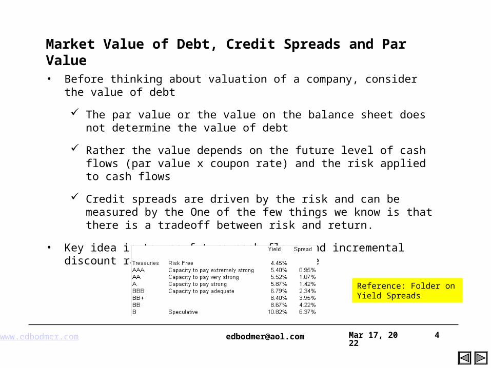
• Before thinking about valuation of a company, consider the value of debt
The par value or the value on the balance sheet does not determine the value of debt
Rather the value depends on the future level of cash flows (par value x coupon rate) and the risk applied to cash flows
Credit spreads are driven by the risk and can be measured by the One of the few things we know is that there is a tradeoff between risk and return.
• Key idea is to use future cash flows and incremental discount rate in measuring market value
Reference: Folder on Yield Spreads
www.edbodmer.com [email protected] Apr 19, 2023 5
Measurement of Risk in Financial Models
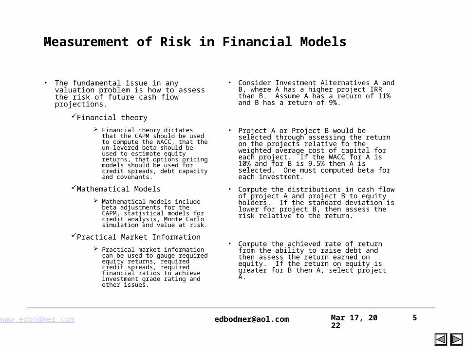
• The fundamental issue in any valuation problem is how to assess the risk of future cash flow projections.
Financial theory
Financial theory dictates that the CAPM should be used to compute the WACC, that the un-levered beta should be used to estimate equity returns, that options pricing models should be used for credit spreads, debt capacity and covenants.
Mathematical Models
Mathematical models include beta adjustments for the CAPM, statistical models for credit analysis, Monte Carlo simulation and value at risk.
Practical Market Information
Practical market information can be used to gauge required equity returns, required credit spreads, required financial ratios to achieve investment grade rating and other issues.
• Consider Investment Alternatives A and B, where A has a higher project IRR than B. Assume A has a return of 11% and B has a return of 9%.
• Project A or Project B would be selected through assessing the return on the projects relative to the weighted average cost of capital for each project. If the WACC for A is 10% and for B is 9.5% then A is selected. One must computed beta for each investment.
• Compute the distributions in cash flow of project A and project B to equity holders. If the standard deviation is lower for project B, then assess the risk relative to the return.
• Compute the achieved rate of return from the ability to raise debt and then assess the return earned on equity. If the return on equity is greater for B then A, select project A.
www.edbodmer.com [email protected] Apr 19, 2023 6
Problems with CAPM
• Ke = Rf + Beta x EMRP
• Difficulty in establishing Rf
• Can’t find Betas
• Betas performed horribly during financial crisis
• EPRM cannot be measured and changes with perceptions over time
www.edbodmer.com [email protected] Apr 19, 2023 7
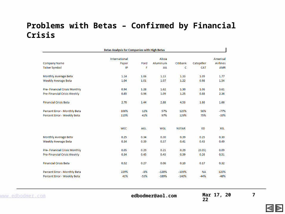
Problems with Betas – Confirmed by Financial Crisis
www.edbodmer.com [email protected] Apr 19, 2023 8
CAPM Post Financial Crisis
• The cost of equity was calculated using the capital asset pricing model, which is a theoretical financial model that estimates the cost of equity capital based on a company’s “beta” which is a measure of a company’s volatility relative to the overall market, a 6% market risk premium and a relevant predicted beta and risk-free rate. The public market trading price targets published by securities research analysts do not necessarily reflect current market trading prices for Wyeth’s and Pfizer’s common stock and these estimates are subject to uncertainties, including the future financial performance of Wyeth and Pfizer and future financial market conditions.
• Academic studies – 2-3%
• Pre-Crisis Bankers – 4-5%
• Historical U.S. premium pre-crisis 6-8%
www.edbodmer.com [email protected] Apr 19, 2023 9
Problems with Growth
• Typical assumption that growth equals inflation means world economy would stop
• Time period before which reach stable growth is impossible to estimate
• Evidence that sell-side analysts chronically over-estimate short-term growth rates
www.edbodmer.com [email protected] Apr 19, 2023 10
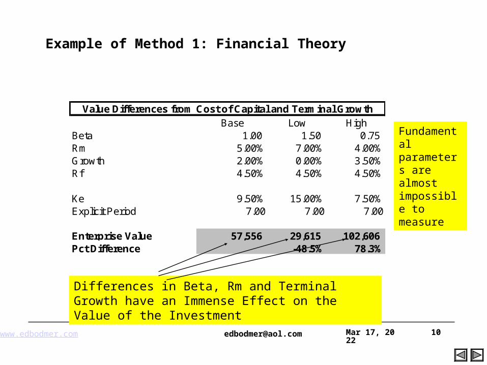
Example of Method 1: Financial Theory
Base Low High
Beta 1.00 1.50 0.75 Rm 5.00% 7.00% 4.00%Growth 2.00% 0.00% 3.50%Rf 4.50% 4.50% 4.50%
Ke 9.50% 15.00% 7.50%Explicit Period 7.00 7.00 7.00
Enterprise Value 57,556 29,615 102,606 Pct Difference -48.5% 78.3%
Value Differences from Cost of Capital and Terminal Growth
Differences in Beta, Rm and Terminal Growth have an Immense Effect on the Value of the Investment
Fundamental parameters are almost impossible to measure
www.edbodmer.com [email protected] Apr 19, 2023 11
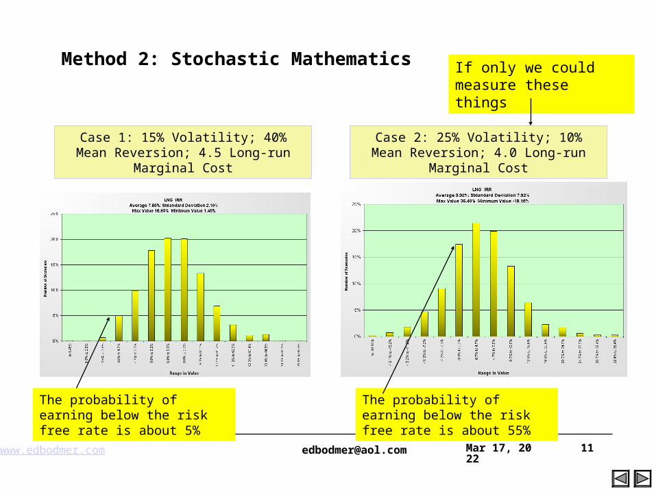
Case 1: 15% Volatility; 40% Mean Reversion; 4.5 Long-run Marginal Cost
Case 2: 25% Volatility; 10% Mean Reversion; 4.0 Long-run Marginal Cost
Method 2: Stochastic Mathematics
The probability of earning below the risk free rate is about 5%
The probability of earning below the risk free rate is about 55%
If only we could measure these things
www.edbodmer.com [email protected] Apr 19, 2023 12
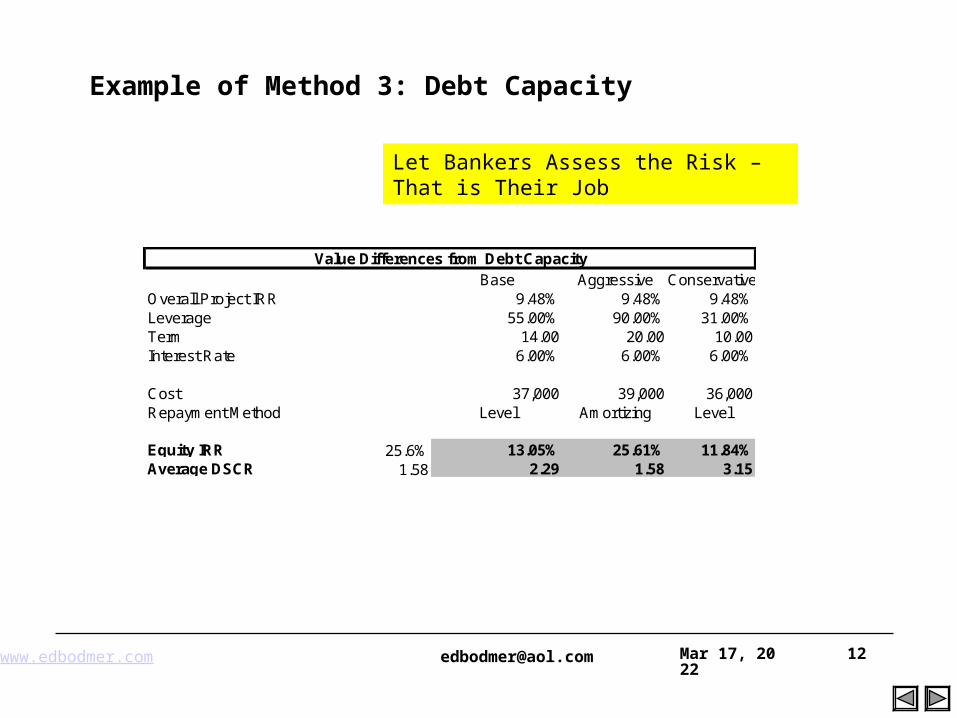
Example of Method 3: Debt Capacity
Base Aggressive ConservativeOverall Project IRR 9.48% 9.48% 9.48%Leverage 55.00% 90.00% 31.00%Term 14.00 20.00 10.00Interest Rate 6.00% 6.00% 6.00%
Cost 37,000 39,000 36,000Repayment Method Level Amortizing Level
Equity IRR 25.6% 13.05% 25.61% 11.84%Average DSCR 1.58 2.29 1.58 3.15
Value Differences from Debt Capacity
Let Bankers Assess the Risk – That is Their Job
www.edbodmer.com [email protected] Apr 19, 2023 13
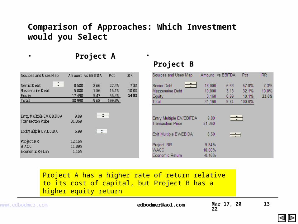
Comparison of Approaches: Which Investment would you Select
• Project A • Project B
Sources and Uses Map Amount vs EBITDA Pct IRR
Senior Debt 8,500 2.66 27.4% 7.3%Mezzenaine Debt 5,000 1.56 16.1% 10.0%Equity 17,490 5.47 56.4% 14.9%Total 30,990 9.68 100.0%
Entry Multiple EV/EBITDA 9.80 Transaction Price 31,360
Exit Multiple EV/EBIDA 6.00
Project IRR 12.16%WACC 11.00%Economic Return 1.16%
Project A has a higher rate of return relative to its cost of capital, but Project B has a higher equity return
www.edbodmer.com [email protected] Apr 19, 2023 14
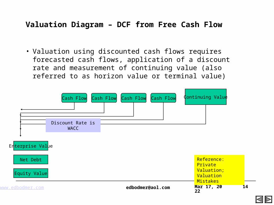
Valuation Diagram – DCF from Free Cash Flow
• Valuation using discounted cash flows requires forecasted cash flows, application of a discount rate and measurement of continuing value (also referred to as horizon value or terminal value)
Cash Flow Cash Flow Cash Flow Cash Flow Continuing Value
Discount Rate is WACC
Enterprise Value
Net Debt
Equity Value
Reference: Private Valuation; Valuation Mistakes
www.edbodmer.com [email protected] Apr 19, 2023 15
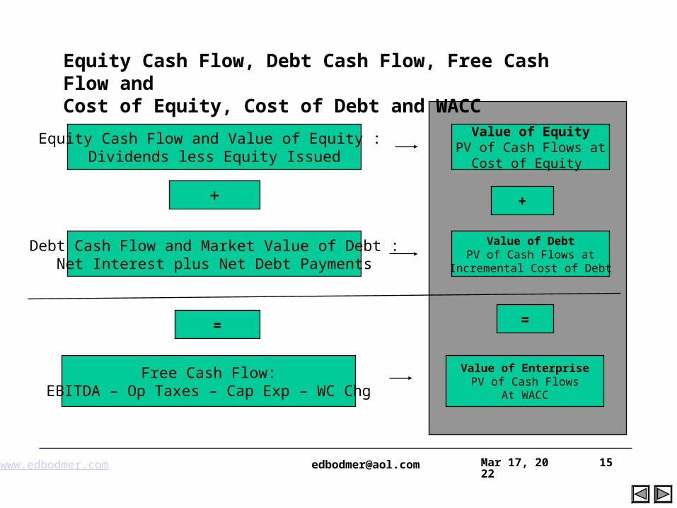
Equity Cash Flow, Debt Cash Flow, Free Cash Flow andCost of Equity, Cost of Debt and WACC
Equity Cash Flow and Value of Equity : Dividends less Equity Issued
Debt Cash Flow and Market Value of Debt :Net Interest plus Net Debt Payments
Free Cash Flow:EBITDA – Op Taxes – Cap Exp – WC Chg
Value of EquityPV of Cash Flows at
Cost of Equity
Value of DebtPV of Cash Flows at
Incremental Cost of Debt
+ +
=
Value of EnterprisePV of Cash Flows
At WACC
=
www.edbodmer.com [email protected] Apr 19, 2023 16
Valuation Overview
Despite that fact that all we have to do is forecast cash flow and then determine the risk associated with those cash flows, valuation is a huge topic. Some Key issues in valuation analysis include:
Cost of Capital in DCF or Discounted Earnings for Measuring Risk
Selection of Market Multiple and Adjustment that implicitly accounts for growth in cash flow and risk
Determination of Growth Rates in Earnings and Cash Flow Projections
How to Compute Terminal Value when Cash Flow Lasts for an Indefinite Period
www.edbodmer.com [email protected] Apr 19, 2023 17
Tools for Valuation
• There is no magic answer as to whether one valuation approach is better than others. But virtually all valuation analyses involve the following work:
• Financial Models:
Valuation model used to project earnings or cash flows
• Statistical Data:
Industry Comparative Data to establish Multiples and Cost of Capital
• Industry, company knowledge and judgment
Knowledge about risks and economic outlook to assess risks and value drivers in the forecasts
www.edbodmer.com [email protected] Apr 19, 2023 18
Problems with Traditional Finance and Discounted Free Cash Flow
• The entire process is dependent on WACC and the CAPM
Rm is one of the most debated issues in finance
Beta is difficult to measure
The model doesn’t work
• Valuation is highly dependent on terminal values and growth rates
Often zero real growth is used, implying that if all companies had zero growth, economies around the world would be stagnant
• If multiples are used, they can be very subjective
Comparable companies are not comparable at all
Arbitrary adjustments are made to the P/E and EV/EBITDA valuation ratios
www.edbodmer.com [email protected] Apr 19, 2023 19
Valuation and Cash Flow
• Ultimately, value comes from cash flow in any model:
DCF – directly measure cash flow from explicit cash flow and cash flow from selling after the explicit period
Multiples – The size of a multiple ultimately depends on cash flow in formulas
FCF/(k-g) = Multiple
They still have implicit cost of capital and growth that must be understood
Replacement Cost – cash from selling assets
• Growth rate in cash flow is a key issue in any of the modelsInvestors cannot buy a house with earnings or use earnings for consumption or investment
www.edbodmer.com [email protected] Apr 19, 2023 20
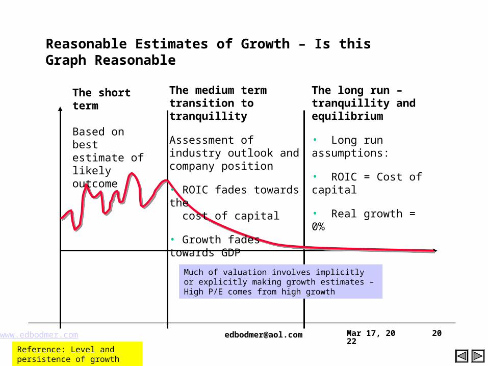
Reasonable Estimates of Growth – Is this Graph Reasonable
The short term
Based on best estimate of likely outcome
The medium term transition to tranquillity
Assessment of industry outlook and company position
• ROIC fades towards the cost of capital
• Growth fades towards GDP
The long run – tranquillity and equilibrium
• Long run assumptions:
• ROIC = Cost of capital
• Real growth = 0%
Much of valuation involves implicitly or explicitly making growth estimates – High P/E comes from high growth
Reference: Level and persistence of growth rates
www.edbodmer.com [email protected] Apr 19, 2023 21
How Long will Growth Last
• Some Theoretical Issues with Growth:
The greater the current growth rate in earnings of a firm, relative to the stable growth rate, the longer the high growth period; although the growth rate may drop off during the period. Thus, a firm that is growing at 40% should have a longer high-growth period than one growing at 14%.
The larger the size of the firm, the shorter the high growth period. Size remains one of the most potent forces that push firms towards stable growth; the larger a firm, the less likely it is to maintain an above-normal growth rate.
The greater the barriers to entry in a business, e.g. patents or strong brand name, should lengthen the high growth period for a firm.
Look at the combination of the three factors A,B,C and make a judgment. Few firms can achieve an expected growth period longer than 10 years
www.edbodmer.com [email protected] Apr 19, 2023 22
Terminal Value and Growth
• Terminal value is reached when a company has reached maturity – it grows at the overall rate of the economy. This should be nominal growth in the economy since all of the currency in models is in nominal terms.
• For immature companies, the reaching of equilibrium will exceed the standard five year forecast
• Extending the forecast forces one to make assumptions for more than one year which become very speculative
• Some suggest a fade growth period to address this issue
www.edbodmer.com [email protected] Apr 19, 2023 23
Fade Period
• The fade period is the length of time it takes for the long-term growth rate to be reached after from the growth in the last year of the forecast.
• For example, the last year growth is 10%
• The terminal growth is 3%
• The time to get from 10% to 3% is 5 years
• You can use the formula
• Growth = Growtht-1 x [(Long term/Short term)]^(1/Fade)
• Note: This does not work with negative growth rates
www.edbodmer.com [email protected] Apr 19, 2023 24
Growth When Companies are Earning More than their Cost of Capital
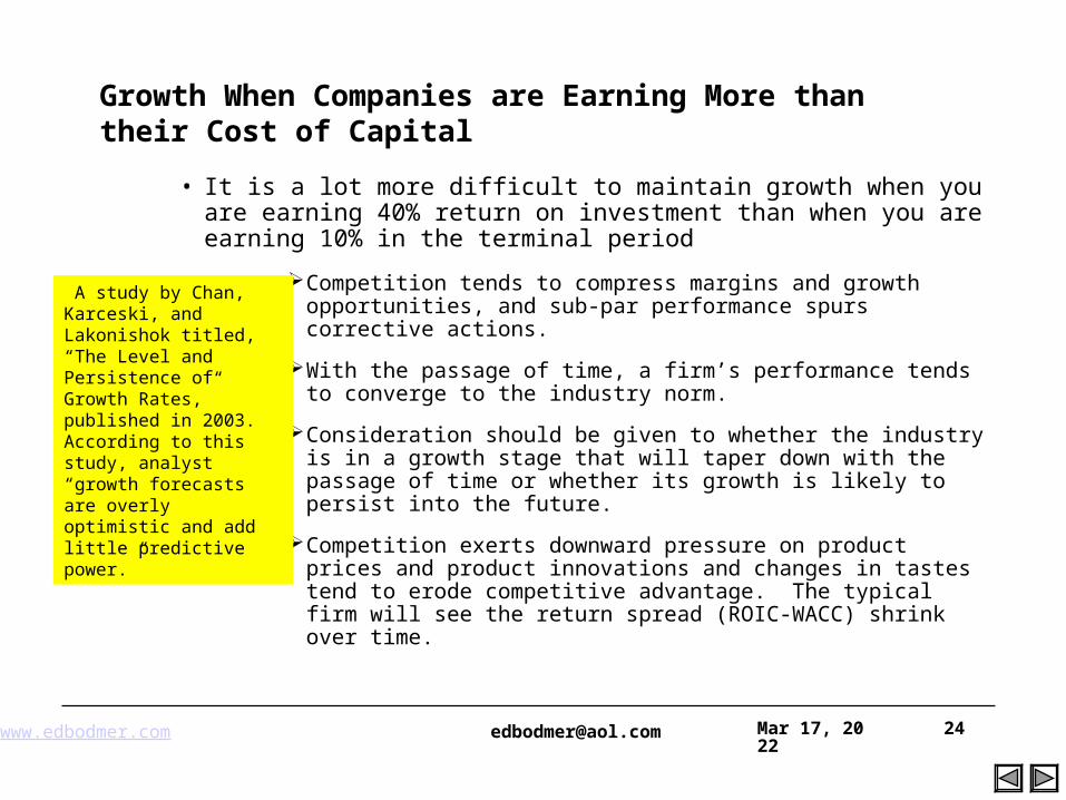
• It is a lot more difficult to maintain growth when you are earning 40% return on investment than when you are earning 10% in the terminal period
Competition tends to compress margins and growth opportunities, and sub-par performance spurs corrective actions.
With the passage of time, a firm’s performance tends to converge to the industry norm.
Consideration should be given to whether the industry is in a growth stage that will taper down with the passage of time or whether its growth is likely to persist into the future.
Competition exerts downward pressure on product prices and product innovations and changes in tastes tend to erode competitive advantage. The typical firm will see the return spread (ROIC-WACC) shrink over time.
A study by Chan, Karceski, and Lakonishok titled, “The Level and Persistence of Growth Rates,” published in 2003. According to this study, analyst “growth forecasts are overly optimistic and add little predictive power.”
www.edbodmer.com [email protected] Apr 19, 2023 25
Growth Issues
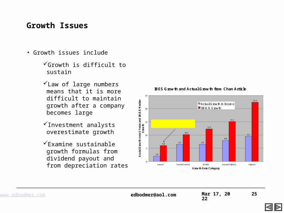
• Growth issues include
Growth is difficult to sustain
Law of large numbers means that it is more difficult to maintain growth after a company becomes large
Investment analysts overestimate growth
Examine sustainable growth formulas from dividend payout and from depreciation rates
IBES Growth and Actual Growth from Chan Article
2.0
6.5 6.5
8.0
9.5
6.0
10.2
12.3
15.1
22.4
0
5
10
15
20
25
Lowest Second Lowest Median Second Highest Highest
Growth Rate Category
Ac
uta
l Gro
wth
ov
er
5 Y
ea
rs a
nd
I/B
/E/S
Me
dia
n
Gro
wth
Actual Growth in IncomeI/B/E/S Growth
Optimism in the lowest growth category is still present.
www.edbodmer.com [email protected] Apr 19, 2023 26
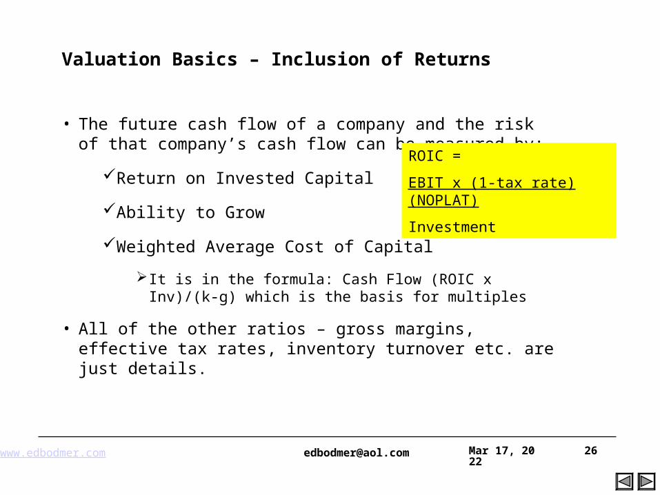
Valuation Basics – Inclusion of Returns
• The future cash flow of a company and the risk of that company’s cash flow can be measured by:
Return on Invested Capital
Ability to Grow
Weighted Average Cost of Capital
It is in the formula: Cash Flow (ROIC x Inv)/(k-g) which is the basis for multiples
• All of the other ratios – gross margins, effective tax rates, inventory turnover etc. are just details.
ROIC =
EBIT x (1-tax rate) (NOPLAT)
Investment
www.edbodmer.com [email protected] Apr 19, 2023 27
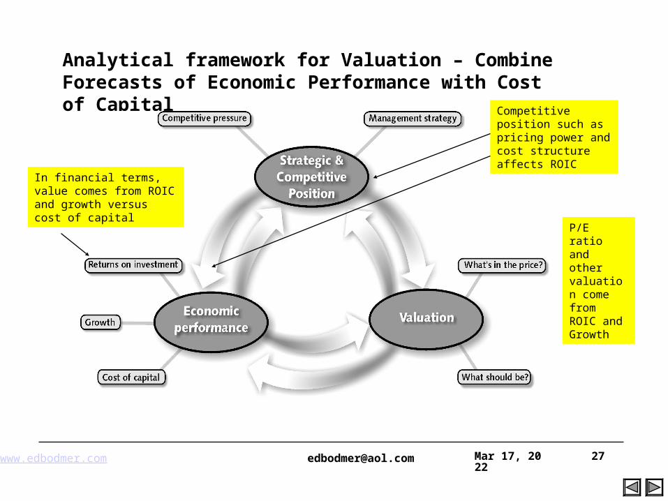
Analytical framework for Valuation – Combine Forecasts of Economic Performance with Cost of Capital
In financial terms, value comes from ROIC and growth versus cost of capital
Competitive position such as pricing power and cost structure affects ROIC
P/E ratio and other valuation come from ROIC and Growth
www.edbodmer.com [email protected] Apr 19, 2023 28
Practical Discounting Issues in Excel
• NPV formula assumes end of period cash flow
• Growth rate is ROE x Retention rate
• If you are selling the stock at the end of the last period and doing a long-term analysis, you must use the next period EBITDA or the next period cash flow.
• If there is growth in a model, you should use the add one year of growth to the last period in making the calculation
• To use mid-year of specific discounting use the IRR or XIRR or sumproduct
www.edbodmer.com [email protected] Apr 19, 2023 29
Valuation and Sustainable Growth
• Value depends on the growth in cash flow. Growth can be estimated using alternative formulas:
Growth in EPS = ROE x (1 – Dividend Payout Ratio)
Growth in Investment = ROIC x (1-Reinvestment Rate)
Growth = (1+growth in units) x (1+inflation) – 1
• When evaluating NOPLAT rather than earnings, a similar concept can be used for sustainable growth.
Growth = (Capital Expenditures/Depreciation – 1) x Depreciation Rate
• Unrealistic to assume growth in units above the growth in the economy on an ongoing basis.
www.edbodmer.com [email protected] Apr 19, 2023 30
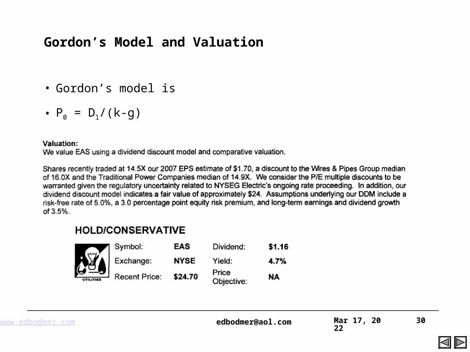
Gordon’s Model and Valuation
• Gordon’s model is
• P0 = D1/(k-g)
• Example
www.edbodmer.com [email protected] Apr 19, 2023 31
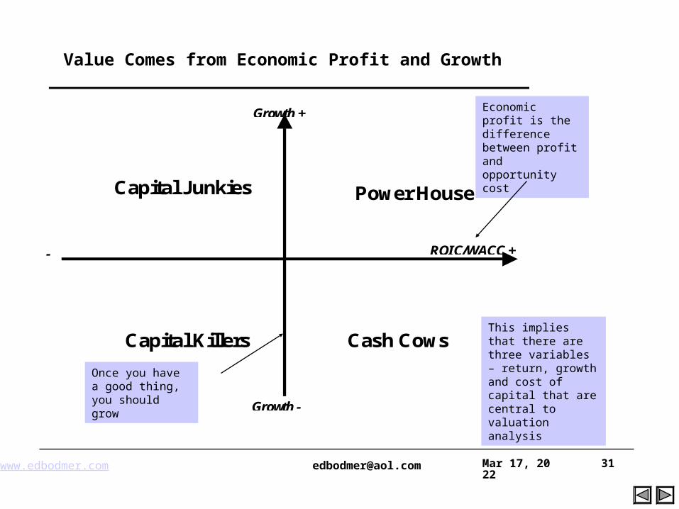
Value Comes from Economic Profit and Growth
Capital Junkies
Power House
Capital Killers
Cash Cows
Growth +
Growth -
ROIC/WACC + ++ve
-
Economic profit is the difference between profit and opportunity cost
Once you have a good thing, you should grow
This implies that there are three variables – return, growth and cost of capital that are central to valuation analysis
www.edbodmer.com [email protected] Apr 19, 2023 32
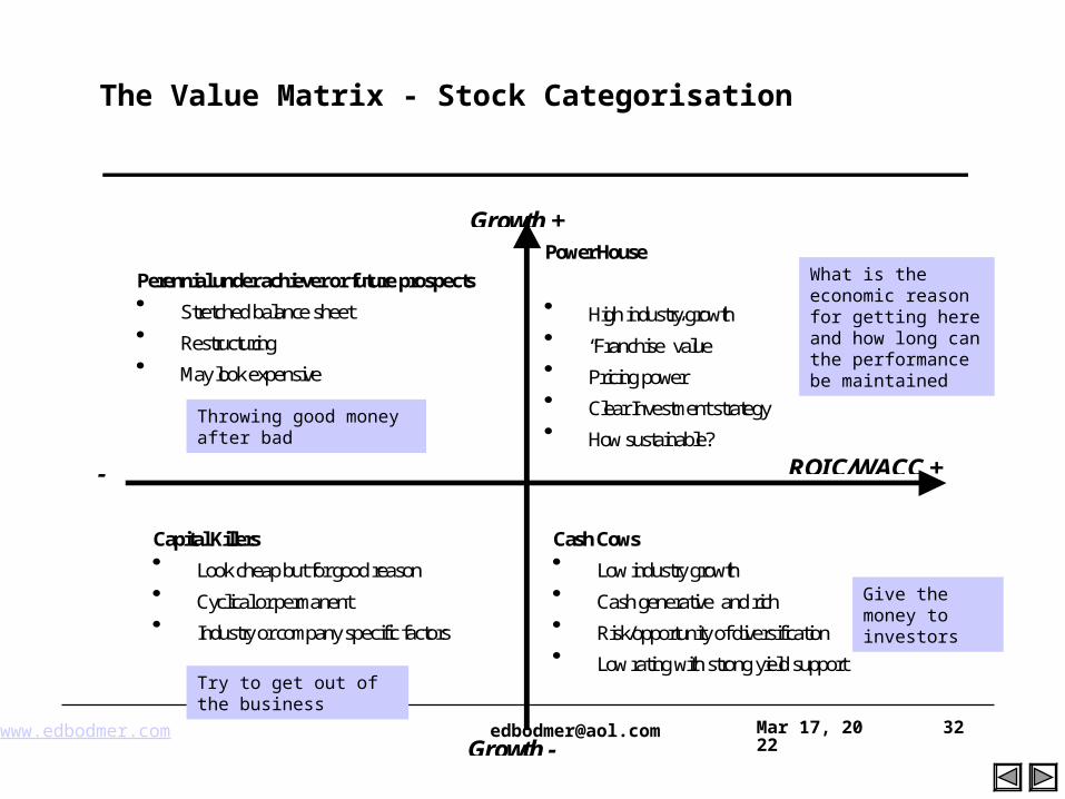
The Value Matrix - Stock Categorisation
Perennial under achiever or future prospects
Stretched balance sheet Restructuring May look expensive
Power House
High industry growth “Franchise” value Pricing power Clear Investment strategy How sustainable?
Capital Killers
Look cheap but for good reason Cyclical or permanent Industry or company specific factors
Cash Cows
Low industry growth Cash generative and rich Risk/opportunity of diversification Low rating with strong yield support
Growth +
Growth -
ROIC/WACC + ++ve
-
Throwing good money after bad
Try to get out of the business
What is the economic reason for getting here and how long can the performance be maintained
Give the money to investors
www.edbodmer.com [email protected] Apr 19, 2023 33
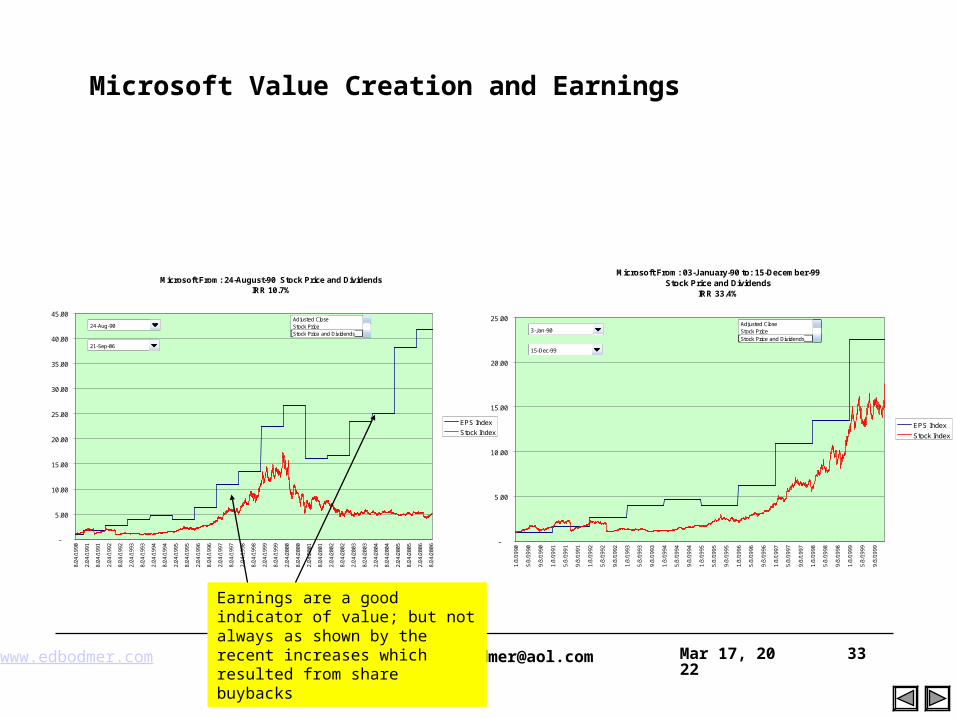
Microsoft Value Creation and Earnings
Microsoft From: 24-August-90 Stock Price and DividendsIRR 10.7%
-
5.00
10.00
15.00
20.00
25.00
30.00
35.00
40.00
45.00
8/24
/199
0
2/24
/199
1
8/24
/199
1
2/24
/199
2
8/24
/199
2
2/24
/199
3
8/24
/199
3
2/24
/199
4
8/24
/199
4
2/24
/199
5
8/24
/199
5
2/24
/199
6
8/24
/199
6
2/24
/199
7
8/24
/199
7
2/24
/199
8
8/24
/199
8
2/24
/199
9
8/24
/199
9
2/24
/200
0
8/24
/200
0
2/24
/200
1
8/24
/200
1
2/24
/200
2
8/24
/200
2
2/24
/200
3
8/24
/200
3
2/24
/200
4
8/24
/200
4
2/24
/200
5
8/24
/200
5
2/24
/200
6
8/24
/200
6
EPS Index
Stock Index
24-Aug-90Adjusted CloseStock PriceStock Price and Dividends
21-Sep-06
Microsoft From: 03-January-90 to: 15-December-99Stock Price and Dividends
IRR 33.4%
-
5.00
10.00
15.00
20.00
25.00
1/3
/199
0
5/3
/199
0
9/3
/199
0
1/3
/199
1
5/3
/199
1
9/3
/199
1
1/3
/199
2
5/3
/199
2
9/3
/199
2
1/3
/199
3
5/3
/199
3
9/3
/199
3
1/3
/199
4
5/3
/199
4
9/3
/199
4
1/3
/199
5
5/3
/199
5
9/3
/199
5
1/3
/199
6
5/3
/199
6
9/3
/199
6
1/3
/199
7
5/3
/199
7
9/3
/199
7
1/3
/199
8
5/3
/199
8
9/3
/199
8
1/3
/199
9
5/3
/199
9
9/3
/199
9
EPS Index
Stock Index
3-Jan-90Adjusted CloseStock PriceStock Price and Dividends
15-Dec-99
Earnings are a good indicator of value; but not always as shown by the recent increases which resulted from share buybacks
www.edbodmer.com [email protected] Apr 19, 2023 34
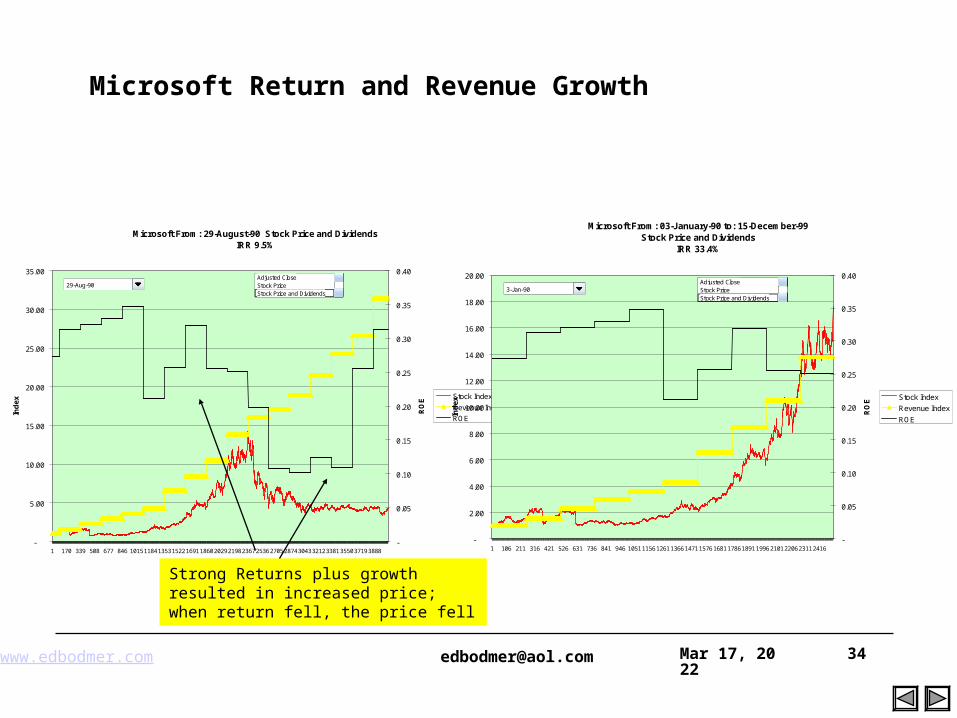
Microsoft Return and Revenue Growth
Microsoft From: 29-August-90 Stock Price and DividendsIRR 9.5%
-
5.00
10.00
15.00
20.00
25.00
30.00
35.00
1 170 339 508 677 846 101511841353152216911860202921982367253627052874304332123381355037193888
Ind
ex
-
0.05
0.10
0.15
0.20
0.25
0.30
0.35
0.40
RO
E
Stock Index
Revenue Index
ROE
29-Aug-90Adjusted CloseStock PriceStock Price and Dividends
Microsoft From: 03-January-90 to: 15-December-99Stock Price and Dividends
IRR 33.4%
-
2.00
4.00
6.00
8.00
10.00
12.00
14.00
16.00
18.00
20.00
1 106 211 316 421 526 631 736 841 946 10511156126113661471157616811786189119962101220623112416
Ind
ex
-
0.05
0.10
0.15
0.20
0.25
0.30
0.35
0.40
RO
E
Stock Index
Revenue Index
ROE
3-Jan-90Adjusted CloseStock PriceStock Price and Dividends
Strong Returns plus growth resulted in increased price; when return fell, the price fell
www.edbodmer.com [email protected] Apr 19, 2023 35
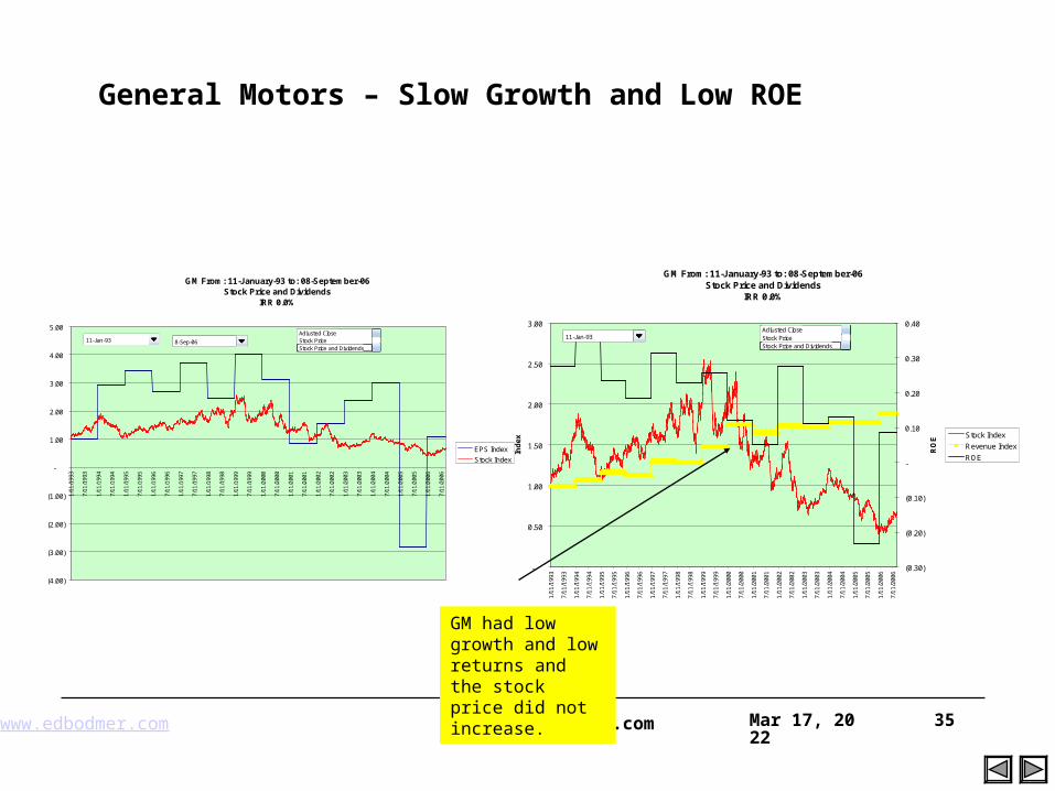
General Motors – Slow Growth and Low ROE
GM From: 11-January-93 to: 08-September-06Stock Price and Dividends
IRR 0.0%
(4.00)
(3.00)
(2.00)
(1.00)
-
1.00
2.00
3.00
4.00
5.00
1/11
/199
3
7/11
/199
3
1/11
/199
4
7/11
/199
4
1/11
/199
5
7/11
/199
5
1/11
/199
6
7/11
/199
6
1/11
/199
7
7/11
/199
7
1/11
/199
8
7/11
/199
8
1/11
/199
9
7/11
/199
9
1/11
/200
0
7/11
/200
0
1/11
/200
1
7/11
/200
1
1/11
/200
2
7/11
/200
2
1/11
/200
3
7/11
/200
3
1/11
/200
4
7/11
/200
4
1/11
/200
5
7/11
/200
5
1/11
/200
6
7/11
/200
6
EPS Index
Stock Index
11-Jan-93Adjusted CloseStock PriceStock Price and Dividends
8-Sep-06
GM From: 11-January-93 to: 08-September-06Stock Price and Dividends
IRR 0.0%
-
0.50
1.00
1.50
2.00
2.50
3.00
1/11
/199
3
7/11
/199
3
1/11
/199
4
7/11
/199
4
1/11
/199
5
7/11
/199
5
1/11
/199
6
7/11
/199
6
1/11
/199
7
7/11
/199
7
1/11
/199
8
7/11
/199
8
1/11
/199
9
7/11
/199
9
1/11
/200
0
7/11
/200
0
1/11
/200
1
7/11
/200
1
1/11
/200
2
7/11
/200
2
1/11
/200
3
7/11
/200
3
1/11
/200
4
7/11
/200
4
1/11
/200
5
7/11
/200
5
1/11
/200
6
7/11
/200
6
Ind
ex
(0.30)
(0.20)
(0.10)
-
0.10
0.20
0.30
0.40
RO
E
Stock Index
Revenue Index
ROE
11-Jan-93Adjusted CloseStock PriceStock Price and Dividends
GM had low growth and low returns and the stock price did not increase.
www.edbodmer.com [email protected] Apr 19, 2023 36
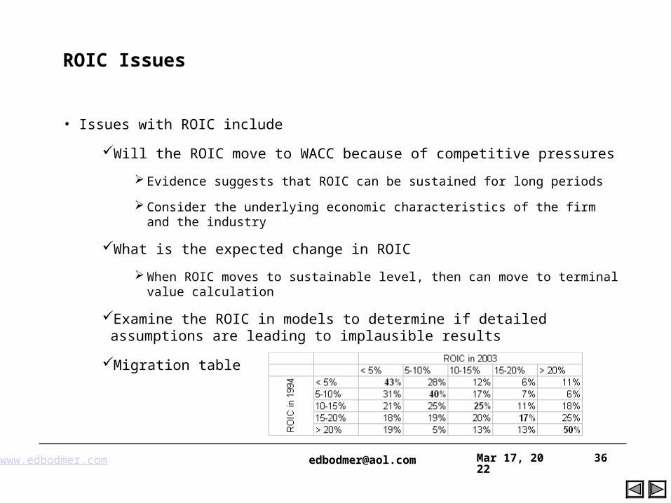
ROIC Issues
• Issues with ROIC include
Will the ROIC move to WACC because of competitive pressures
Evidence suggests that ROIC can be sustained for long periods
Consider the underlying economic characteristics of the firm and the industry
What is the expected change in ROIC
When ROIC moves to sustainable level, then can move to terminal value calculation
Examine the ROIC in models to determine if detailed assumptions are leading to implausible results
Migration table
www.edbodmer.com [email protected] Apr 19, 2023 37
• What we really need to estimate are reinvestment rates and marginal returns on equity and capital in the future (the change in income over the change in equity).
• Those who use analyst’s or historical growth rates are implicitly assuming something about reinvestment rates and returns, but they are either unaware of these assumptions or do not make them explicit. This means, look at the ROE and the dividends to make sure that the growth is consistent.
• Future ROE depends on changes in economic variables affecting the existing investment and new projects with incremental returns.
Practical Growth Rate Issues: Growth Rate Estimation vs. ROE and Retention Rate
ValuationApr 19, 202338
Alternative Valuation Methods
www.edbodmer.com [email protected] Apr 19, 2023 39
Valuation Ranges
• Do not claim to derive a single number – unrealistic to derive one number
Forecasting uncertainty
Cost of capital uncertainty
Bigger ranges for growth companies and for emerging economies
www.edbodmer.com [email protected] Apr 19, 2023 40
General Valuation Approaches
• Typical Valuation Approaches are Differentiated According to:
Relative Valuation
Multiples, Comparative Transactions
Absolute Valuation
DCF, APV, Risk Neutral Valuation, Option Pricing
• We Differentiate by
Direct Valuation
DCF, Multiples etc.
Indirect Valuation
Equity IRR from LBO Multiples, Accretion/Dilution in EPS from integrated merger analysis, IRR and debt capacity in project finance
www.edbodmer.com [email protected] Apr 19, 2023 41
Direct Valuation Models
• There are many valuation techniques for assets and investments including:
Income Approach
Discounted Cash Flow
Venture Capital method
Risk Neutral Valuation
Sales Approach
Multiples (financial ratios) from Comparable Public Companies of from Transactions or from Theoretical Analysis
Liquidation Value
Cost Approach
Replacement Cost (New) and Reproduction Cost of similar assets
Other
Break-up Value
Options Pricing
• The different techniques should give consistent valuation answersSee the appraisal folder in the financial library
www.edbodmer.com [email protected] Apr 19, 2023 42
Indirect Valuation from Modelling Transactions
• Instead of using DCF or multiples, back into the value of a company:
Leveraged buyout
Entry and exit multiples, debt capacity and EBITDA Growth. See how much you can pay an finance and obtain an equity rate or return consistent general benchmarks such as 20%.
Project Finance
Given contracts and assumptions about cash flows over the life of the asset and debt capacity, see how much investment can be made to generate and equity rate of return.
Merger Integration
Given assumptions about financing and accounting in a mergers, see how much you can afford to pay and still achieve accretion in earnings per share.
www.edbodmer.com [email protected] Apr 19, 2023 43
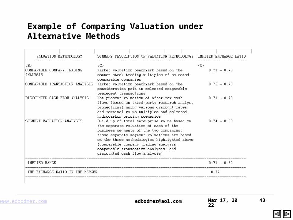
Example of Comparing Valuation under Alternative Methods
www.edbodmer.com [email protected] Apr 19, 2023 44
Sum of the Parts Analysis
• Morgan Stanley performed a sum of the parts analysis, which is designed to imply a value of a company based on the separate valuation of the company’s business segments. Morgan Stanley calculated ranges of implied equity values per share for Wyeth, assuming a hypothetical disposition of Wyeth’s Nutrition, Consumer and Animal Health divisions.
• Morgan Stanley valued Wyeth’s divisions using multiple ranges derived from comparable precedent transactions.
• Morgan Stanley used a 3.5x to 4.5x multiple of aggregate value to estimated 2008 revenue for Wyeth’s Nutrition and Consumer divisions, and
• 11.0x to 13.0x multiple of aggregate value to estimated 2009 EBITDA for the Animal Health division.
• The Pharmaceutical division was valued at a public market trading multiple range of 9.0x to 11.0x estimated 2009 P/E multiple.
• Based on the multiple ranges described above, and including the net present value of the step-up in the tax basis of the assets which would result from such a theoretical transaction, this analysis implied a range for Wyeth’s common stock of approximately $33 to $40 per share. Morgan Stanley noted that the merger consideration had an implied value of $50.19 per share.
www.edbodmer.com [email protected] Apr 19, 2023 45
Risk Neutral Valuation
• Theory – If one can establish value with one financial strategy, the value should be the same as the value with alternative approaches
• In risk neutral valuation, an arbitrage strategy allows one to use the risk free rate in valuing hedged cash flows.
• Forward markets are used to create arbitrage
• Risk neutral valuation does not work with risks that cannot be hedged
• Use risk free rate on hedged cash flow
• Example
Valuation of Oil Production Company
Costs Known
No Future Capital Expenditures
www.edbodmer.com [email protected] Apr 19, 2023 46
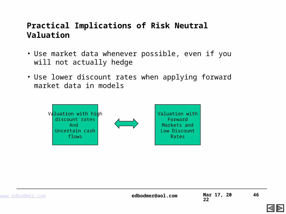
Practical Implications of Risk Neutral Valuation
• Use market data whenever possible, even if you will not actually hedge
• Use lower discount rates when applying forward market data in models
Valuation with highdiscount rates
And Uncertain cash
flows
Valuation withForward
Markets andLow Discount
Rates
www.edbodmer.com [email protected] Apr 19, 2023 47
Examples of Risk Neutral Valuation
• Risk neutral valuation means that one attempts to remove the risk from the cash flow and then discount the adjusted cash flow at the risk free rate. (This is how options pricing models were developed.)
• There are various examples of risk neutral valuation that can be applied in valuation:
If there is a construction contract that includes a premium – say 20% to eliminate cost over-run and delay risk; this verifies the risk rather than attempts to simulate the risk or use of a high discount rate.
If there is a long-term contract that fixes the price, the project can be financed with a lower discount rate.
If a project can secure political risk insurance to eliminate political and currency conversion risk, a lower discount rate can be used rather than attempting to measure political risk.
Other examples …
www.edbodmer.com [email protected] Apr 19, 2023 48
Venture Capital Method
• Two Cash Flows
Investment (Negative)
IPO Terminal Value (Positive)
Terminal Value = Value at IPO x Share of Company Owned
• Valuation of Terminal Value
Discount Rates of 50% to 75%
Risky cash flows
Other services
See the article on private valuation
www.edbodmer.com [email protected] Apr 19, 2023 49
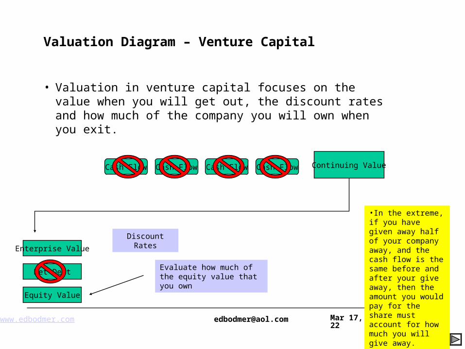
Valuation Diagram – Venture Capital
• Valuation in venture capital focuses on the value when you will get out, the discount rates and how much of the company you will own when you exit.
Cash Flow Cash Flow Cash Flow Cash Flow Continuing Value
Discount Rates
Enterprise Value
Net Debt
Equity Value
Evaluate how much of the equity value that you own
•In the extreme, if you have given away half of your company away, and the cash flow is the same before and after your give away, then the amount you would pay for the share must account for how much you will give away.
www.edbodmer.com [email protected] Apr 19, 2023 50
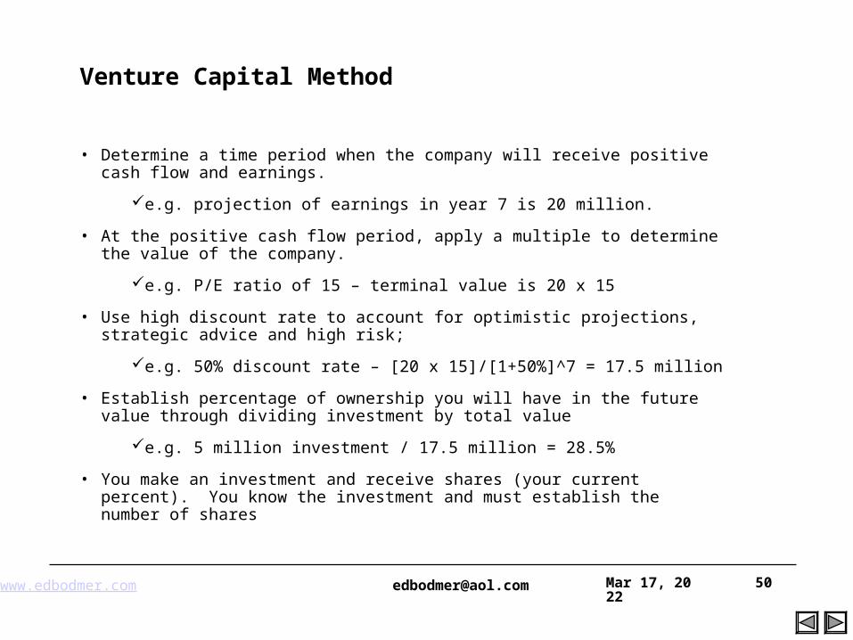
Venture Capital Method
• Determine a time period when the company will receive positive cash flow and earnings.
e.g. projection of earnings in year 7 is 20 million.
• At the positive cash flow period, apply a multiple to determine the value of the company.
e.g. P/E ratio of 15 – terminal value is 20 x 15
• Use high discount rate to account for optimistic projections, strategic advice and high risk;
e.g. 50% discount rate – [20 x 15]/[1+50%]^7 = 17.5 million
• Establish percentage of ownership you will have in the future value through dividing investment by total value
e.g. 5 million investment / 17.5 million = 28.5%
• You make an investment and receive shares (your current percent). You know the investment and must establish the number of shares
www.edbodmer.com [email protected] Apr 19, 2023 51
Venture Capital Method Continued
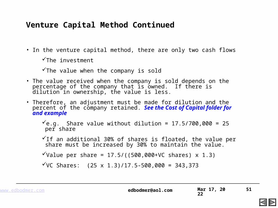
• In the venture capital method, there are only two cash flows
The investment
The value when the company is sold
• The value received when the company is sold depends on the percentage of the company that is owned. If there is dilution in ownership, the value is less.
• Therefore, an adjustment must be made for dilution and the percent of the company retained. See the Cost of Capital folder for and example
e.g. Share value without dilution = 17.5/700,000 = 25 per share
If an additional 30% of shares is floated, the value per share must be increased by 30% to maintain the value.
Value per share = 17.5/((500,000+VC shares) x 1.3)
VC Shares: (25 x 1.3)/17.5-500,000 = 343,373
www.edbodmer.com [email protected] Apr 19, 2023 52
Replacement Cost
• First a couple of points regarding replacement cost theory
In theory, one can replace the assets of a company without investing in the company. If you are valuing a company, you may think about creating the company yourself.
If you replaced a company and really measured the replacement cost, the value of the company may be more than replacement cost because the company manages the assets better than you could.
By replacing the assets and entering the business, you would receive cash flows. You can reconcile the replacement cost with the discounted cash flow approach
www.edbodmer.com [email protected] Apr 19, 2023 53
Measuring Replacement Cost
• Replacement cost includes:
Value of hard assets
Value of patents and other intangibles
Cost of recruiting and training management
• Analysis
Begin with balance sheet categories, account for the age of the plant
Add: cost of hiring and training management
• If the company is generating more cash flow than that would be produced from replacement cost, the management may be more productive than others in managing costs or be able to realize higher prices through differentiation of products.
• The ratio of market value to replacement cost is a theoretical ratio that measures the value of management contribution
www.edbodmer.com [email protected] Apr 19, 2023 54
Replacement Value and Tobin’s Q
• Recall Tobin’s Q as:
Q = Enterprise Value / Replacement Cost
• Buy assets and talent etc and should receive the ROIC. Earn industry average ROIC.
If the ROIC > industry average, then Q > 1.
If the ROIC < industry average, then Q < 1
www.edbodmer.com [email protected] Apr 19, 2023 55
Real Options in Investment Decisions
• Example of real options in many investments
the right to abandon an asset in the research and development phase;
the right to abandon the plant during construction;
the right to delay construction of the facility;
the right not to dispatch the plant when prices below short-run marginal cost;
the right to retire or mothball the plant before the end of its physical life;
the right to extend the life of the plant instead of retiring it at the end of its planned life; and
the right to expand the asset
www.edbodmer.com [email protected] Apr 19, 2023 56
Real Options and Problems with DCF
• The DCF model has many conceptual flaws, the most significant of which is assuming that cash flows are normally distributed around the mean or base case level.
• For many investments, the cash flows are skewed:
When an asset is to be retired, there is more upside than downside because the asset will continue to operate when times are good, but it will be scrapped when times are bad.
An investment decision often involves the possibility to expand in the future. When the expansion decision is made, it will only occur when the economics are good.
During the period of constructing an asset, it is possible to cancel the construction expenditures and limit the downside if it becomes clear that the project will not be economic.
www.edbodmer.com [email protected] Apr 19, 2023 57
Real Options and DCF Problems - Continued
• Problems with DCF because of flexibility in managing assets:
In operating an asset, the asset can be shut down when it is not economic and re-started when it becomes economic. This allows the asset to retain the upside but not incur negative cash flows.
When developing a project, there is a possibility to abandon the project that can limit the downside as more becomes known about the economics of the project.
In deciding when to construct an investment, one can delay the investment until it becomes clear that the decision is economic. This again limits the downside cash flows.
• In each of these cases, management flexibility provides protection in the downside which means that DCF model produces biased results.
www.edbodmer.com [email protected] Apr 19, 2023 58
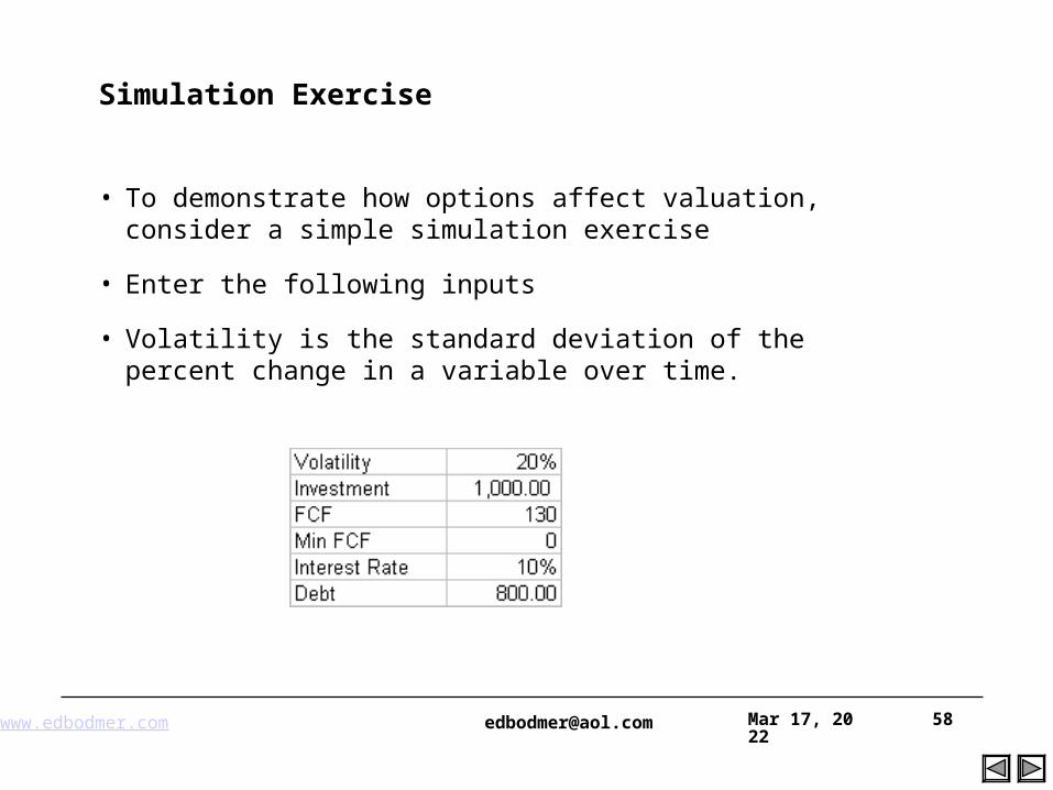
Simulation Exercise
• To demonstrate how options affect valuation, consider a simple simulation exercise
• Enter the following inputs
• Volatility is the standard deviation of the percent change in a variable over time.
www.edbodmer.com [email protected] Apr 19, 2023 59
Fundamental Valuation
• What was behind the bull market of 1980-1999
EPS rose from 15 to 56
Nominal growth of 6.9% -- about the growth in the real economy (the real GDP)
Keeping P/E constant would have large share price increase
Long-term interest rates fell – lower cost of capital increases the P/E ratio
• Real Market
Value by ROIC versus growth
Select strategies that lead to economic profit
Market value from expected performance
www.edbodmer.com [email protected] Apr 19, 2023 60
Three Primary Methods Discussed in Remainder of Slides
• Market Multiples – Relative Valuation
• Discounted Free Cash Flow
• Discounted Earnings and Dividends
• Warning: No method is perfect or completely precise
• Use industry expertise and judgment in assessing discount rates and multiples
• Different valuation methods should yield similar results
• Bangor Hydro Case
ValuationApr 19, 202361
Discounting Basics
www.edbodmer.com [email protected] Apr 19, 2023 62
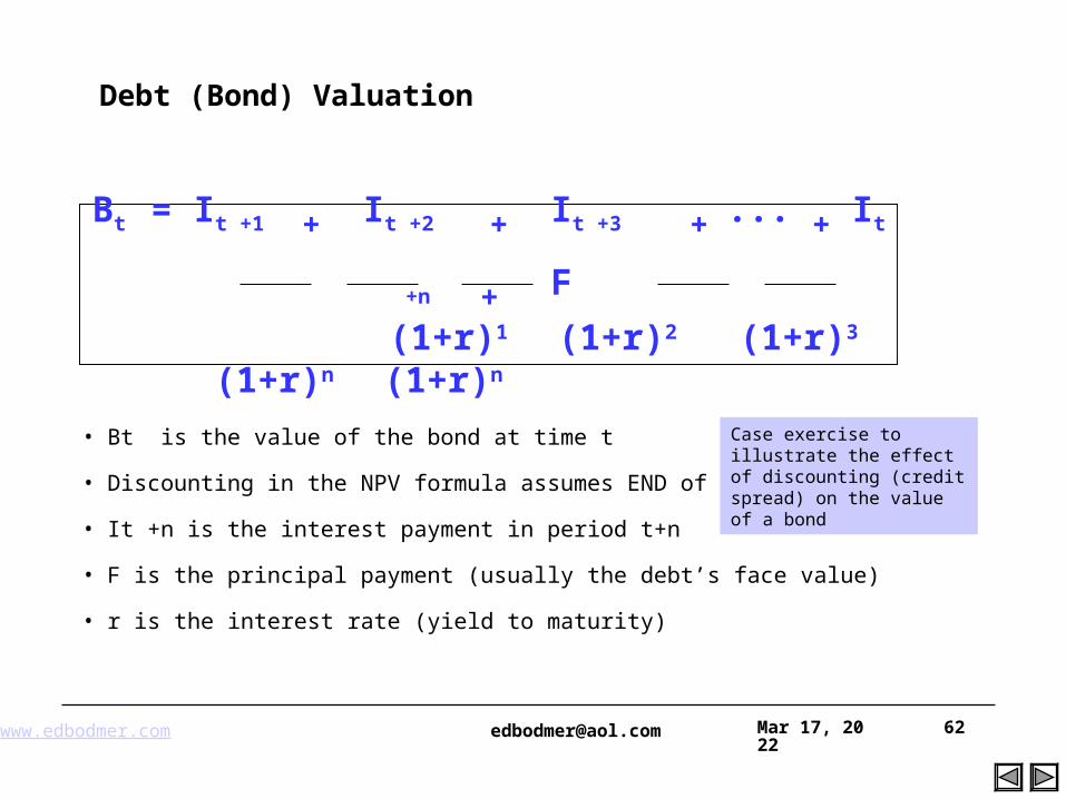
Bt = It +1 + It +2 + It +3 + ... + It +n + F
(1+r)1 (1+r)2 (1+r)3 (1+r)n (1+r)n
Debt (Bond) Valuation
• Bt is the value of the bond at time t
• Discounting in the NPV formula assumes END of period
• It +n is the interest payment in period t+n
• F is the principal payment (usually the debt’s face value)
• r is the interest rate (yield to maturity)
Case exercise to illustrate the effect of discounting (credit spread) on the value of a bond
www.edbodmer.com [email protected] Apr 19, 2023 63
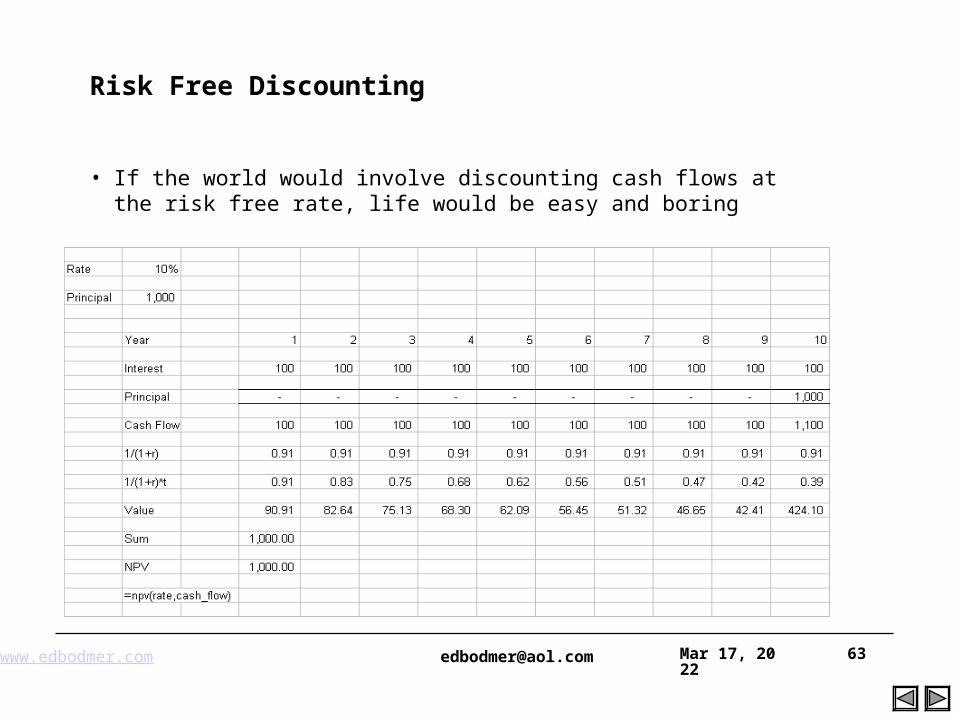
Risk Free Discounting
• If the world would involve discounting cash flows at the risk free rate, life would be easy and boring
www.edbodmer.com [email protected] Apr 19, 2023 64
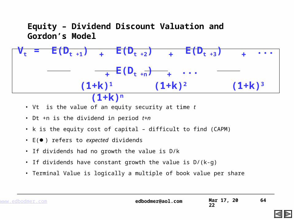
Vt = E(Dt +1) + E(Dt +2) + E(Dt +3) + ... + E(Dt +n) + ...
(1+k)1 (1+k)2 (1+k)3 (1+k)n
Equity – Dividend Discount Valuation and Gordon’s Model
• Vt is the value of an equity security at time t
• Dt +n is the dividend in period t+n
• k is the equity cost of capital – difficult to find (CAPM)
• E() refers to expected dividends
• If dividends had no growth the value is D/k
• If dividends have constant growth the value is D/(k-g)
• Terminal Value is logically a multiple of book value per share
www.edbodmer.com [email protected] Apr 19, 2023 65
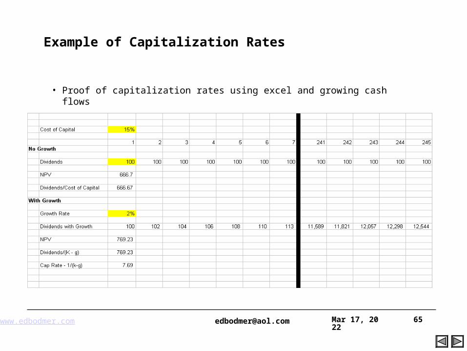
Example of Capitalization Rates
• Proof of capitalization rates using excel and growing cash flows
www.edbodmer.com [email protected] Apr 19, 2023 66
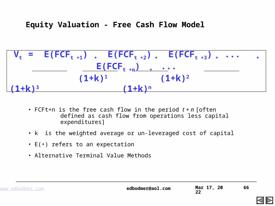
Vt = E(FCFt +1) + E(FCFt +2) + E(FCFt +3) + ... + E(FCFt +n) + ... (1+k)1 (1+k)2 (1+k)3 (1+k)n
• FCFt+n is the free cash flow in the period t + n [often defined as cash flow from operations less capital
expenditures]
• k is the weighted average or un-leveraged cost of capital
• E(•) refers to an expectation
• Alternative Terminal Value Methods
Equity Valuation - Free Cash Flow Model
www.edbodmer.com [email protected] Apr 19, 2023 67
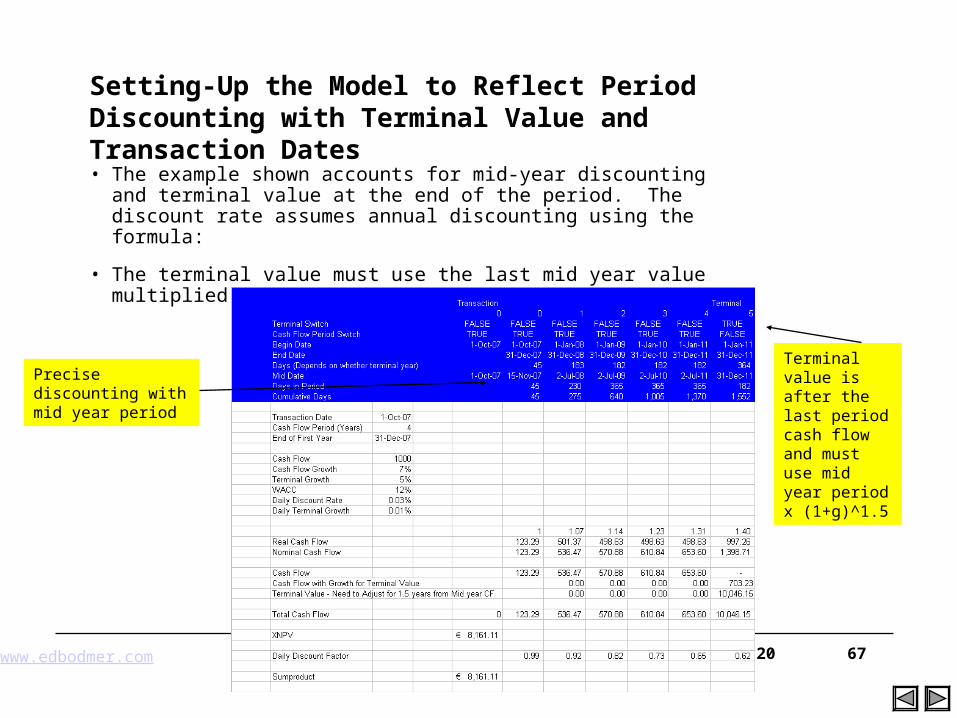
Setting-Up the Model to Reflect Period Discounting with Terminal Value and Transaction Dates
• The example shown accounts for mid-year discounting and terminal value at the end of the period. The discount rate assumes annual discounting using the formula:
• The terminal value must use the last mid year value multiplied by (1+g)^1.5
Precise discounting with mid year period
Terminal value is after the last period cash flow and must use mid year period x (1+g)^1.5
ValuationApr 19, 202368
Valuation Using Multiples
www.edbodmer.com [email protected] Apr 19, 2023 69
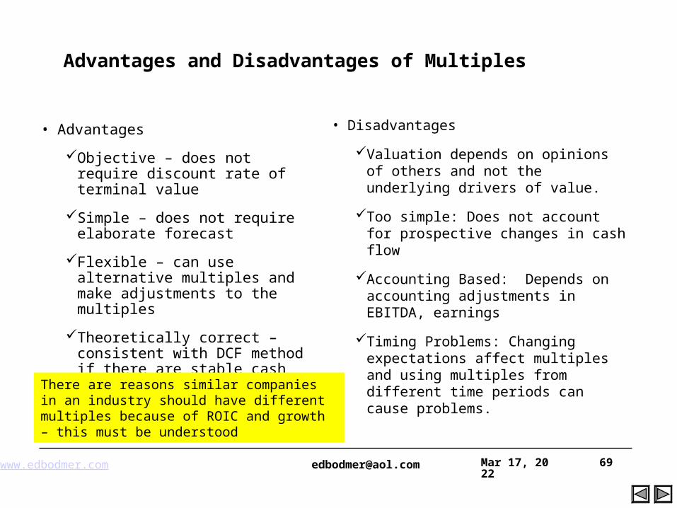
Advantages and Disadvantages of Multiples
• Advantages
Objective – does not require discount rate of terminal value
Simple – does not require elaborate forecast
Flexible – can use alternative multiples and make adjustments to the multiples
Theoretically correct – consistent with DCF method if there are stable cash flows and constant growth – FCF/(k-g).
• Disadvantages
Valuation depends on opinions of others and not the underlying drivers of value.
Too simple: Does not account for prospective changes in cash flow
Accounting Based: Depends on accounting adjustments in EBITDA, earnings
Timing Problems: Changing expectations affect multiples and using multiples from different time periods can cause problems.
There are reasons similar companies in an industry should have different multiples because of ROIC and growth – this must be understood
www.edbodmer.com [email protected] Apr 19, 2023 70
Equity Analysis – Target Prices
• Equity Research Analyst Price Targets Analysis
• Morgan Stanley reviewed and analyzed future public market trading price targets for Wyeth’s common stock and Pfizer’s common stock prepared and published by equity research analysts. These targets reflect each analyst’s estimate of the future public market trading price of Wyeth’s common stock and Pfizer’s common stock. Morgan Stanley noted that the range of equity analyst price targets of Wyeth’s common stock was between approximately $33 and $48 per share. Morgan Stanley further calculated that using a cost of equity of 8.5% and a discount period of one year, the present value of the equity analyst price target range for Wyeth’s common stock was approximately $30 to $44 per share, with a mean target price of $40.82 and a median target price of $40.00. Morgan Stanley noted that the merger consideration had an implied value of $50.19 per share of Wyeth’s common stock based upon $17.45 per share of Pfizer common stock, the closing price of Pfizer’s common stock on January 23, 2009, the last trading day prior to announcement of the proposed merger.
www.edbodmer.com [email protected] Apr 19, 2023 71
Example of Problems with Relative Valuation – Housing Prices
• During the housing bubble, appraisers would use the value of similar transactions to estimate the value of properties
Appraisers would have a lot of tricks and make biased estimates by using houses with relatively high value and ignoring those with lower value (if they did not make high estimates, they would not be hired)
The fundamentals of housing value from evaluating the income levels relative to the house price, the trends in housing or the demand and supply of housing were ignored.
This lead to absurd valuations.
www.edbodmer.com [email protected] Apr 19, 2023 72
Valuation from Multiples
• Valuation from multiples is known as relative valuation because valuation is compared to other companies and not to fundamental cash flows.
• A measure of value is standardized by earnings or something else
Financial Multiples
P/E Ratio
EV/EBITDA
Price/Book
Industry Specific
Value/Oil Reserve
Value/Subscriber
Value/Square Foot
Issues
Where to find the multiple data and comparable companies
What income or cash flow base to use
Discounts for lack of marketability
www.edbodmer.com [email protected] Apr 19, 2023 73
Mechanics of Multiples
• Find market multiple from comparable companies
Rarely are there truly comparable companies
Understand economics that drive multiples (growth rate, cost of capital and return)
• P/E Ratio (forward versus trailing)
Value/Share = P/E x Projected EPS
P/E trailing and forward multiples
• Market to Book
Value/Share = Market to Book Ratio x Book Value/Share
• EV/EBITDA
Value/Share = (EV/EBITDA x EBITDA – Debt) divided by shares
• P/E and M/B use equity cash flow; EV/EBITDA uses free cash flow
In the long-term P/E ratios tend to revert to a mean of 15.0
www.edbodmer.com [email protected] Apr 19, 2023 74
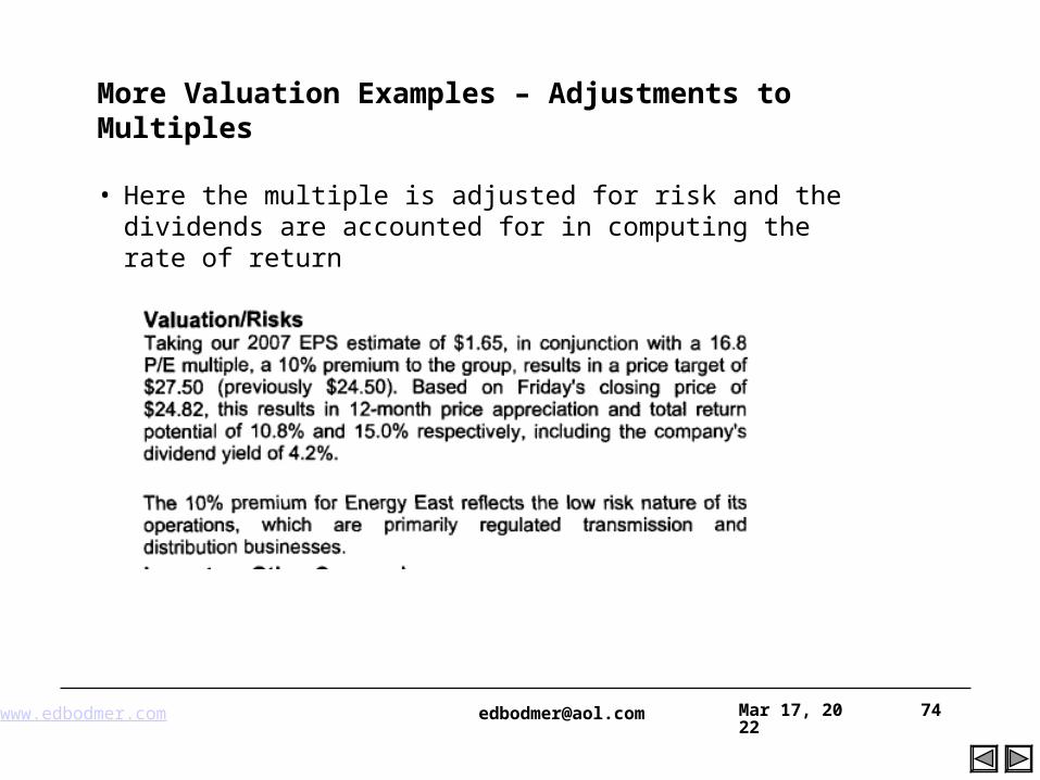
More Valuation Examples – Adjustments to Multiples
• Here the multiple is adjusted for risk and the dividends are accounted for in computing the rate of return
www.edbodmer.com [email protected] Apr 19, 2023 75
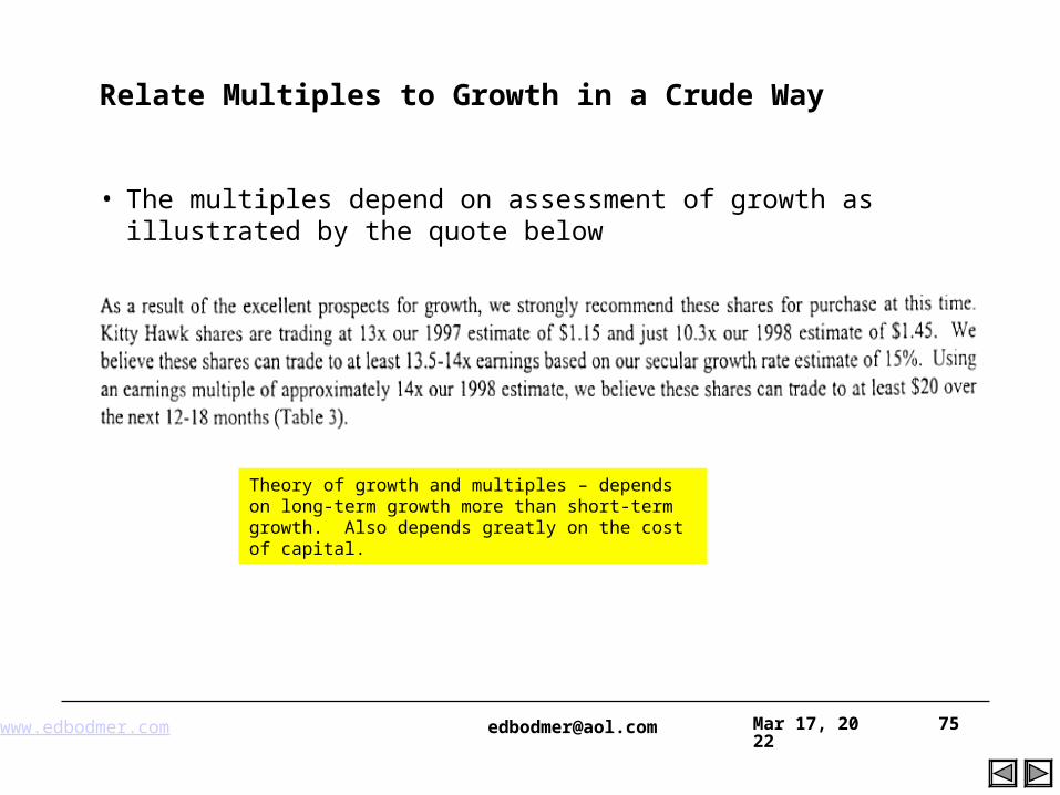
Relate Multiples to Growth in a Crude Way
• The multiples depend on assessment of growth as illustrated by the quote below
Theory of growth and multiples – depends on long-term growth more than short-term growth. Also depends greatly on the cost of capital.
www.edbodmer.com [email protected] Apr 19, 2023 76
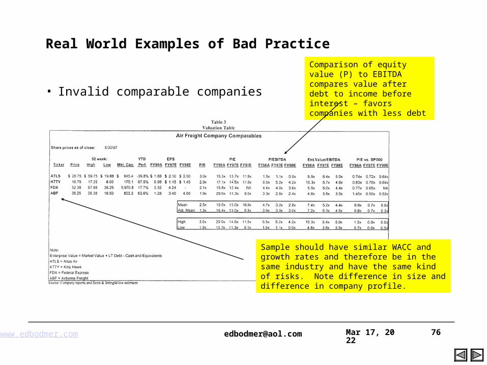
Real World Examples of Bad Practice
• Invalid comparable companies
• Logical comparisons
Sample should have similar WACC and growth rates and therefore be in the same industry and have the same kind of risks. Note difference in size and difference in company profile.
Comparison of equity value (P) to EBITDA compares value after debt to income before interest – favors companies with less debt
www.edbodmer.com [email protected] Apr 19, 2023 77
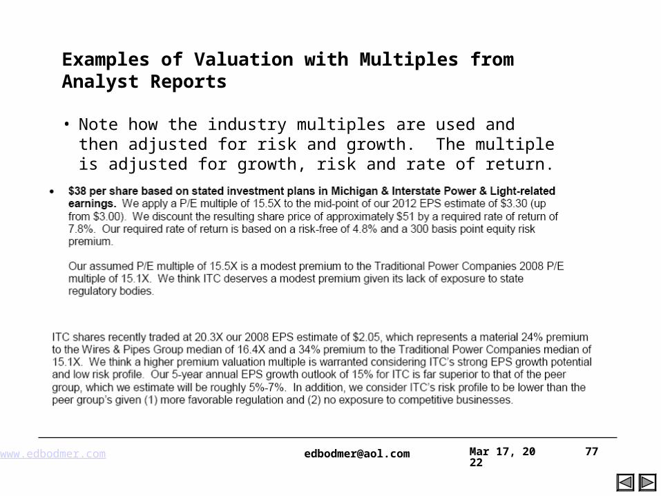
Examples of Valuation with Multiples from Analyst Reports
• Note how the industry multiples are used and then adjusted for risk and growth. The multiple is adjusted for growth, risk and rate of return.

www.edbodmer.com [email protected] Apr 19, 2023 78
Use of Multiples in Valuation
The red bars from the DCF valuation are compared to market date
Should be able to explain difference from:
1.Growth
2. WACC
3. ROIC
www.edbodmer.com [email protected] Apr 19, 2023 79
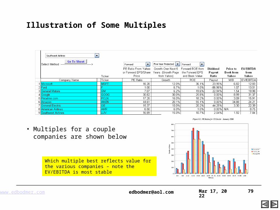
Illustration of Some Multiples
• Multiples for a couple companies are shown below
Which multiple best reflects value for the various companies – note the EV/EBITDA is most stable
www.edbodmer.com [email protected] Apr 19, 2023 83
Which Multiple to Use
• Valuation from multiples uses information from other companies
• It is relevant when the company is already in a steady state situation and there is no reason to expect that you can improve estimates of EBITDA or Earnings
• One of the challenges is to understand which multiple works in which situation:
Leveraged Buyout
EV/EBITDA is used
Changes in the common equity ratio Intangible assets make book value inappropriate Different leverage makes P/E difficult
Banks/Insurance
Market/Book may be best
Not many intangible assets, so book value is meaningful Book value is the value of loans which is adjusted with loan loss provisions Cost of capital and financing is very important because of the cost of
deposits
www.edbodmer.com [email protected] Apr 19, 2023 84
Multiples - Summary
• Useful sanity check for valuation from other methods
• Use multiples to avoid subjective forecasts
• Among other things, well done multiple that accounts for
Accounting differences
Inflation effects
Cyclicality
• Use appropriate comparable samples
• Use forward P/E rather than trailing
• Comprehensive analysis of multiples is similar to forecast
• Use forecasts to explain why multiples are different for a specific company
When you compute the terminal value using
CF x (1+g)/(k-g)
Compute the implied
EV/EBITDA from the data
Also compute the implied P/E and the implied EV/EBITDA when computing the DCF
www.edbodmer.com [email protected] Apr 19, 2023 85
P/E Ratio, Growth and Reconciliation to Cash Flow
• P = D1/(k-g)
• g = ROE * (1-DPO) or DPO = 1 - g/ROE
• P/E = D/E/(k-g)
• Substituting for D/E = DPO
• P/E = (1-g/r)/(k-g)
g -- long term growth rate in earnings and cash flow
r -- rate of return earned on new investment
k -- discount rate
• (k-g) = (1-g/r)/(P/E)
• k = (1-g/r)/(P/E) + g
• Example: if r = k than the formula boils down to 1/(k)
• If the g = 0, the formula is P/E = 1/k
www.edbodmer.com [email protected] Apr 19, 2023 86
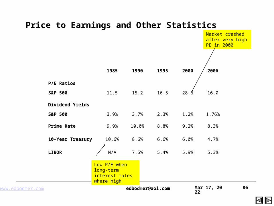
Price to Earnings and Other Statistics
1985 1990 1995 2000 2006
P/E Ratios
S&P 500 11.5 15.2 16.5 28.6 16.0
Dividend Yields
S&P 500 3.9% 3.7% 2.3% 1.2% 1.76%
Prime Rate 9.9% 10.0% 8.8% 9.2% 8.3%
10-Year Treasury 10.6% 8.6% 6.6% 6.0% 4.7%
LIBOR N/A 7.5% 5.4% 5.9% 5.3%
Market crashed after very high PE in 2000
Low P/E when long-term interest rates where high
www.edbodmer.com [email protected] Apr 19, 2023 87
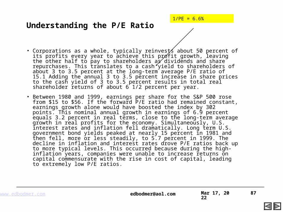
Understanding the P/E Ratio
• Corporations as a whole, typically reinvests about 50 percent of its profits every year to achieve this profit growth, leaving the other half to pay to shareholders as dividends and share repurchases. This translates to a cash yield to shareholders of about 3 to 3.5 percent at the long-term average P/E ratio of 15.1 Adding the annual 3 to 3.5 percent increase in share prices to the cash yield of 3 to 3.5 percent results in total real shareholder returns of about 6 1/2 percent per year.
• Between 1980 and 1999, earnings per share for the S&P 500 rose from $15 to $56. If the forward P/E ratio had remained constant, earnings growth alone would have boosted the index by 302 points. This nominal annual growth in earnings of 6.9 percent equals 3.2 percent in real terms, close to the long-term average growth in real profits for the economy. Simultaneously, U.S. interest rates and inflation fell dramatically. Long term U.S. government bond yields peaked at nearly 15 percent in 1981 and then fell, more or less steadily, to 5.7 percent in 1999. The decline in inflation and interest rates drove P/E ratios back up to more typical levels. This occurred because during the high-inflation years, companies were unable to increase returns on capital commensurate with the rise in cost of capital, leading to extremely low P/E ratios.
1/PE = 6.6%
www.edbodmer.com [email protected] Apr 19, 2023 88
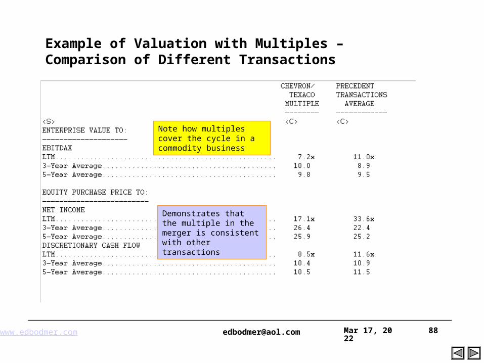
Example of Valuation with Multiples – Comparison of Different Transactions
Demonstrates that the multiple in the merger is consistent with other transactions
Note how multiples cover the cycle in a commodity business
www.edbodmer.com [email protected] Apr 19, 2023 89
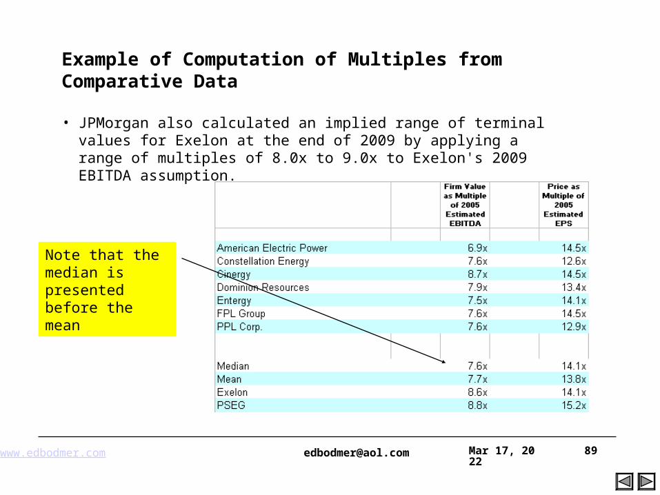
Example of Computation of Multiples from Comparative Data
• JPMorgan also calculated an implied range of terminal values for Exelon at the end of 2009 by applying a range of multiples of 8.0x to 9.0x to Exelon's 2009 EBITDA assumption.
Note that the median is presented before the mean
www.edbodmer.com [email protected] Apr 19, 2023 90
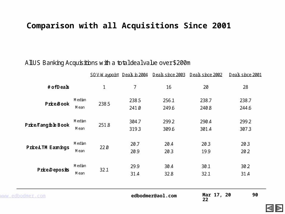
Comparison with all Acquisitions Since 2001
All US Banking Acquisitions with a total deal value over $200m
SOV-Waypoint Deals in 2004 Deals since 2003 Deals since 2002 Deals since 2001
# of Deals 1 7 16 20 28
Median 238.5 256.1 238.7 238.7Mean 241.0 249.6 240.8 244.6
Median 304.7 299.2 290.4 299.2Mean 319.3 309.6 301.4 307.3
Median 20.7 20.4 20.3 20.3Mean 20.9 20.3 19.9 20.2
Median 29.9 30.4 30.1 30.2Mean 31.4 32.8 32.1 31.4
238.5
251.8
22.0
32.1
Price/Book
Price/Tangible Book
Price/LTM Earnings
Price/Deposits
www.edbodmer.com [email protected] Apr 19, 2023 91
Adjustments to Multiples
• Process
Find multiples from similar public companies
Adjust multiples for
Liquidity
Size
Control premium
Developing country discount
Apply adjusted multiples to book value, earnings, and EBITDA
• There is often more money in dispute in determining the discounts and premiums in a business valuation than in arriving at the pre-discount valuation itself. Discounts and premiums affect not only the value of the company, but also play a crucial role in determining the risk involved, control issues, marketability, contingent liability, and a host of other factors.
www.edbodmer.com [email protected] Apr 19, 2023 92
• If the entity were closely held with no (or little) active market for the shares or interest in the company, then a non-marketability discount would be subtracted from the value.
• Non-marketabiliy Discounts – ranges from 10% to 30%
• …represents the reduction in value from a marketable interest level of value to compensate an investor for illiquidity of the security, all else equal.
• The size of the discount varies base on:
relative liquidity (such as the size of the shareholder base);
the dividend yield, expected growth in value and holding period;
and firm specific issues such as imminent or pending initial public offering (IPO) of stock to be freely traded on a public market.
Adjustments to Multiples – Marketability and Liquidity Discount
www.edbodmer.com [email protected] Apr 19, 2023 93
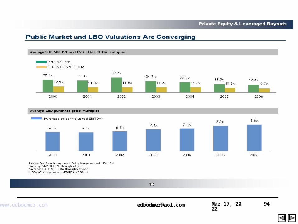
Studies of Liquidity Discount
• Private and public transactions
Attempt to compute EV/EBITDA in public and private transactions
Adjust so that the transactions are comparable
Compute the ratio in pubic and private transactions
Discount of 20 to 28 percent for US firms
Discount of 44 to 54 percent for non-US firms
• Other studies
Value in IPO versus value of private trades before IPO
High liquidity in 40-50% range, but selection bias
Theory involves control by public board
www.edbodmer.com [email protected] Apr 19, 2023 94
www.edbodmer.com [email protected] Apr 19, 2023 95
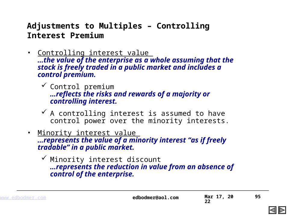
• Controlling interest value …the value of the enterprise as a whole assuming that the stock is freely traded in a public market and includes a control premium.
Control premium …reflects the risks and rewards of a majority or controlling interest.
A controlling interest is assumed to have control power over the minority interests.
• Minority interest value …represents the value of a minority interest “as if freely tradable” in a public market.
Minority interest discount …represents the reduction in value from an absence of control of the enterprise.
Adjustments to Multiples – Controlling Interest Premium
www.edbodmer.com [email protected] Apr 19, 2023 96
21
18
25
16
24
17
20
1819
15
17
13
20
16
21
19
23
17
25
17
24
21
0
5
10
15
20
25
30
1996 1997 1998 1999 2000 2001 2002 2003 2004 2005 2006
Public Private
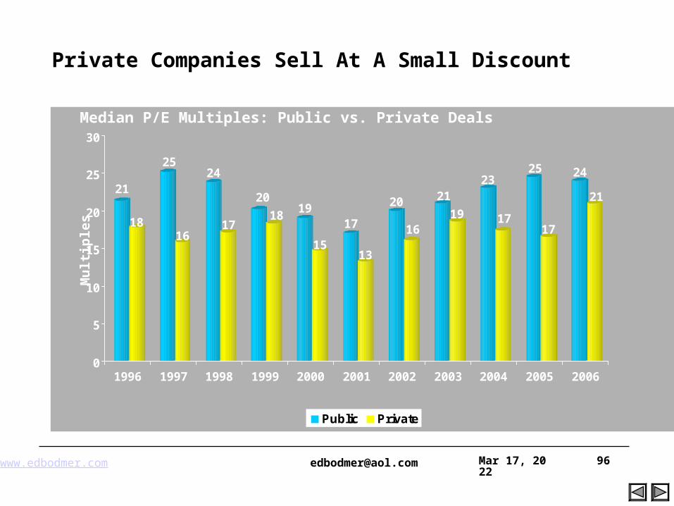
Private Companies Sell At A Small Discount
Median P/E Multiples: Public vs. Private Deals
Mu
ltip
les
Source: Mergerstat (U.S. Only)Disclaimer: Data is continually updated and is subject to change
www.edbodmer.com [email protected] Apr 19, 2023 97
9.610.0
10.9
8.8
11.4
12.8
8.3
11.111.6
8.29.2
10.3
7.7
9.3
11.1
6.9
9.38.4
7.0
8.69.4
7.88.8
11.3
9.49.9
11.8
9.19.9
11.8
8.5
11.4 11.3
0
2
4
6
8
10
12
14
1996 1997 1998 1999 2000 2001 2002 2003 2004 2005 2006
Under $250 Million $250 to $500 Million Over $500 Million
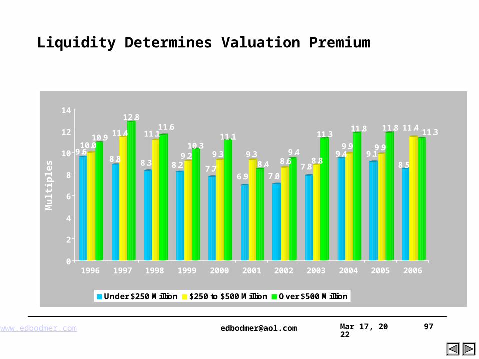
Liquidity Determines Valuation Premium
Median Transaction Multiples by Deal Size
Mu
ltip
les
Source: Mergerstat (U.S. Only)Disclaimer: Data is continually updated and is subject to change
www.edbodmer.com [email protected] Apr 19, 2023 98
P/E Analysis – Use of P/E Ratio in Valuation
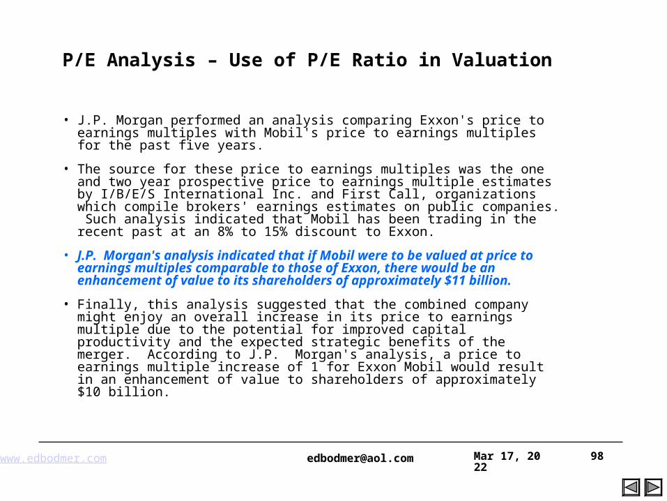
• J.P. Morgan performed an analysis comparing Exxon's price to earnings multiples with Mobil's price to earnings multiples for the past five years.
• The source for these price to earnings multiples was the one and two year prospective price to earnings multiple estimates by I/B/E/S International Inc. and First Call, organizations which compile brokers' earnings estimates on public companies. Such analysis indicated that Mobil has been trading in the recent past at an 8% to 15% discount to Exxon.
• J.P. Morgan's analysis indicated that if Mobil were to be valued at price to earnings multiples comparable to those of Exxon, there would be an enhancement of value to its shareholders of approximately $11 billion.
• Finally, this analysis suggested that the combined company might enjoy an overall increase in its price to earnings multiple due to the potential for improved capital productivity and the expected strategic benefits of the merger. According to J.P. Morgan's analysis, a price to earnings multiple increase of 1 for Exxon Mobil would result in an enhancement of value to shareholders of approximately $10 billion.
www.edbodmer.com [email protected] Apr 19, 2023 99
P/E Ratio, Growth and Reconciliation to Cash Flow
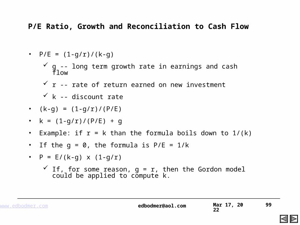
• P/E = (1-g/r)/(k-g)
g -- long term growth rate in earnings and cash flow
r -- rate of return earned on new investment
k -- discount rate
• (k-g) = (1-g/r)/(P/E)
• k = (1-g/r)/(P/E) + g
• Example: if r = k than the formula boils down to 1/(k)
• If the g = 0, the formula is P/E = 1/k
• P = E/(k-g) x (1-g/r)
If, for some reason, g = r, then the Gordon model could be applied to compute k.
www.edbodmer.com [email protected] Apr 19, 2023 100
Company Profile in website
• http://finance.yahoo.com/
• http://googlefinance.com/
• http://marketwatch.com/
• http://bloomberg.com/
• http://pages.stern.nyu.edu/~adamodar/
www.edbodmer.com [email protected] Apr 19, 2023 101
Price Earnings Ratio
• The price earnings ratio is obviously very important in stock evaluation. Therefore, I describe some background related to the ratio and some theory with regards to the P/E ratio. Subjects related to the P/E ratio include:
Dividend growth Model
Theory of price earnings ratio and growth
P/E ratio and the EV/EBITDA ratio
The PE ratio depends more on accounting
The PE is affected by leverage
The EV/EBITDA ignores depreciation and capital expenditure
Case exercise on P/E and EV/EBITDA
www.edbodmer.com [email protected] Apr 19, 2023 102
P/E Ratio versus EV/EBITDA
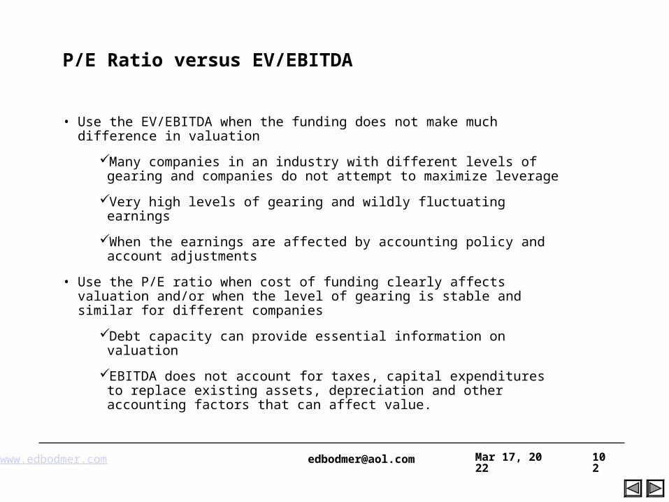
• Use the EV/EBITDA when the funding does not make much difference in valuation
Many companies in an industry with different levels of gearing and companies do not attempt to maximize leverage
Very high levels of gearing and wildly fluctuating earnings
When the earnings are affected by accounting policy and account adjustments
• Use the P/E ratio when cost of funding clearly affects valuation and/or when the level of gearing is stable and similar for different companies
Debt capacity can provide essential information on valuation
EBITDA does not account for taxes, capital expenditures to replace existing assets, depreciation and other accounting factors that can affect value.
www.edbodmer.com [email protected] Apr 19, 2023 103
P/E Ratio
• If you use the P/E ratio for valuation, the ratio implies that only this year or last years earnings matter
• Cash matters to investors in the end, not earnings (different lifetime of earnings)
• When earnings reflect cash flow, P/E is reasonable for valuation
• High P/E causes treadmill and does not necessary imply that companies are performing well
• Earnings can be managed and manipulated
www.edbodmer.com [email protected] Apr 19, 2023 104
Use of P/E Ratio Formula to Compute the Required Return on Equity Capital
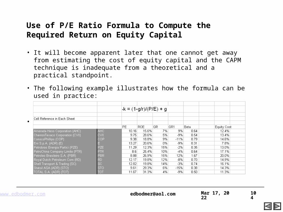
• It will become apparent later that one cannot get away from estimating the cost of equity capital and the CAPM technique is inadequate from a theoretical and a practical standpoint.
• The following example illustrates how the formula can be used in practice:
k = (1-g/r)/(P/E) + g
•
www.edbodmer.com [email protected] Apr 19, 2023 105
P/E Notes
• High ROE does not mean high PE – Hence the existence of high ROE stocks with low PEs
• Growth and value are not always positively correlated
• Growth from improvement will always be value enhancing whereas growth from reinvestment depends upon the return against the benchmark return
• Reinvestment should also include “ Cash hoarding”
• PB is better at differentiating ROE differences than PE
www.edbodmer.com [email protected] Apr 19, 2023 106
Relationship Between Multiples
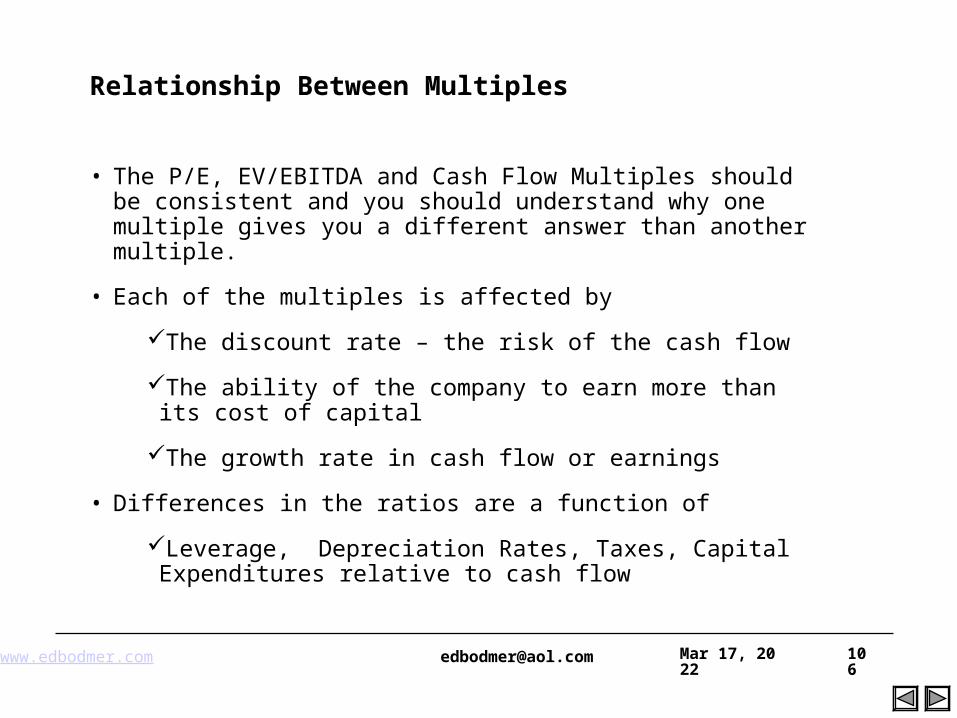
• The P/E, EV/EBITDA and Cash Flow Multiples should be consistent and you should understand why one multiple gives you a different answer than another multiple.
• Each of the multiples is affected by
The discount rate – the risk of the cash flow
The ability of the company to earn more than its cost of capital
The growth rate in cash flow or earnings
• Differences in the ratios are a function of
Leverage, Depreciation Rates, Taxes, Capital Expenditures relative to cash flow
www.edbodmer.com [email protected] Apr 19, 2023 107
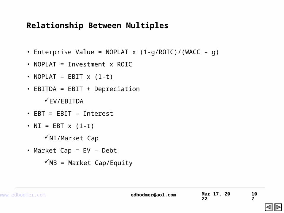
Relationship Between Multiples
• Enterprise Value = NOPLAT x (1-g/ROIC)/(WACC – g)
• NOPLAT = Investment x ROIC
• NOPLAT = EBIT x (1-t)
• EBITDA = EBIT + Depreciation
EV/EBITDA
• EBT = EBIT – Interest
• NI = EBT x (1-t)
NI/Market Cap
• Market Cap = EV – Debt
MB = Market Cap/Equity
www.edbodmer.com [email protected] Apr 19, 2023 108
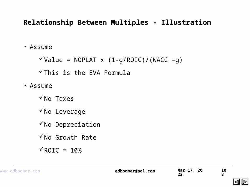
Relationship Between Multiples - Illustration
• Assume
Value = NOPLAT x (1-g/ROIC)/(WACC –g)
This is the EVA Formula
• Assume
No Taxes
No Leverage
No Depreciation
No Growth Rate
ROIC = 10%
www.edbodmer.com [email protected] Apr 19, 2023 109
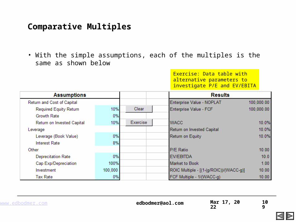
Comparative Multiples
• With the simple assumptions, each of the multiples is the same as shown below
Exercise: Data table with alternative parameters to investigate P/E and EV/EBITA
www.edbodmer.com [email protected] Apr 19, 2023 110
Comparative Multiples
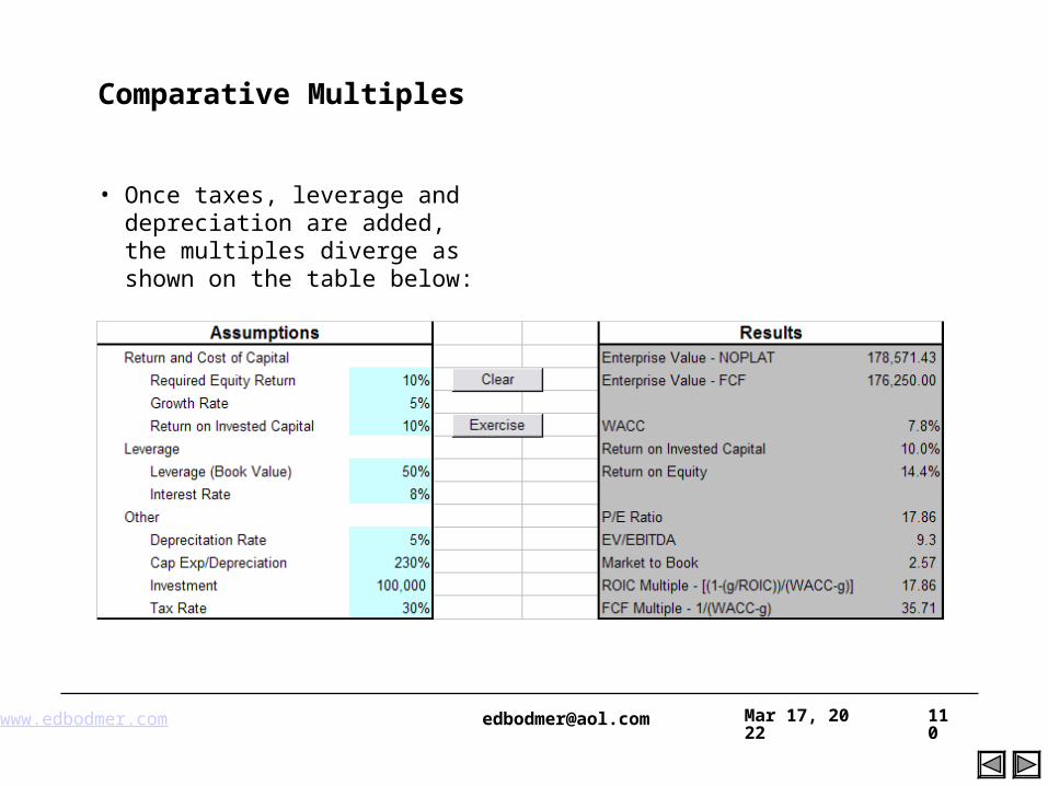
• Once taxes, leverage and depreciation are added, the multiples diverge as shown on the table below:

ValuationApr 19, 2023111
Valuation From Discounted Free Cash Flow
www.edbodmer.com [email protected] Apr 19, 2023 112
Advantages and Disadvantages of DCF
• Advantages
Theoretically Valid – value comes from free cash flow and assessing risk of the free cash flow.
Operating and Financial Values – explicitly separates value from operating the company with value of financial obligations and value from cash
Sensitivity – forces an understanding of key drivers of the business and allows sensitivity and scenario analysis
Fundamental – not biased by optimism or pessimism in the market
• Disadvantages
Assumptions: Requires WACC assumptions and residual value assumptions. There are major problems with WACC estimation and the long-term growth assumption.
Forecasting Problems: Complex forecasting models can easily be manipulated
Growth: The residual value depends on a number of assumptions which can easily distort value
Real Options: Discussed above
www.edbodmer.com [email protected] Apr 19, 2023 113
Problems with DCF – Range in Values
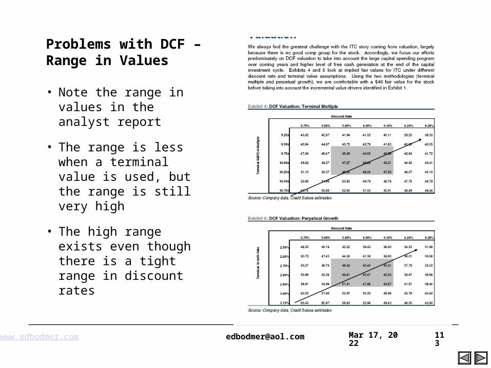
• Note the range in values in the analyst report
• The range is less when a terminal value is used, but the range is still very high
• The high range exists even though there is a tight range in discount rates
www.edbodmer.com [email protected] Apr 19, 2023 114
Discounted Cash Flow – Morgan Stanley Example
• Morgan Stanley performed a discounted cash flow analysis, which is designed to imply a value of a company by calculating the present value of estimated future cash flows of the company.
• Morgan Stanley calculated ranges of implied equity values per share for Wyeth, based on discounted cash flow analyses utilizing Wall Street analyst estimates compiled by Thomson First Call and Wyeth management projections for the calendar years 2009 through 2013. In arriving at the estimated equity values per share of Wyeth’s common stock, Morgan Stanley calculated a terminal value by applying a range of perpetual free cash flow growth rates ranging from (0.5)% to 0.5%.
• Such rate range was derived, based on Morgan Stanley’s judgment, after considering a number of factors, including growth of the overall economy, projected earnings expectations for comparable pharmaceutical companies and Wyeth’s upcoming patent expiration profile.
• Morgan Stanley observed that this range implied P/E multiples for Wyeth that were consistent with the P/E multiples of the comparable companies studied by Morgan Stanley and identified above under “— Comparable Companies Analysis.” The unlevered free cash flows and the terminal value were then discounted to present values using a range of weighted average cost of capital from 7.0% to 9.0%.
• Morgan Stanley selected this range using the capital asset pricing model. The weighted average cost of capital is a measure of the average expected return on all of a given company’s equity securities and debt based on their proportions in such company’s capital structure.
www.edbodmer.com [email protected] Apr 19, 2023 115
Discounted Cash Flow – General Discussion
• Executives and investors alike can draw reassurance from an important trend that has gained momentum even through years of the market's twists and turns. More and more investors, analysts, and investment bankers are turning to fundamental financial analysis and sophisticated discounted cash flow (DCF) models as the touchstone of corporate valuation.
• Recent accounting scandals and inappropriate calculation of revenues and capital expenses give DCF new importance. With heightened concerns over the quality of earnings and reliability of standard valuation metrics like P/E ratios, more investors are turning to free cash flow, which offers a more transparent metric for gauging performance than earnings. It is harder to fool the cash register. Developing a DCF model demands a lot more work than simply dividing the share price by earnings or sales. But in return for the effort, investors get a good picture of the key drivers of share value: expected growth in operating earnings, capital efficiency, balance sheet capital structure, cost of equity and debt, and expected duration of growth. An added bonus is that DCF is less likely to be manipulated by aggressive accounting practices.
www.edbodmer.com [email protected] Apr 19, 2023 116
Discounted Flow
• Use the discounted cash flow when you know something more about the company that can be obtained with a forecast
• Any cash flow forecast involves:
Value =
Cash flow during explicit forecast period +
Present of cash flow after explicit forecast period
• The second item generally involves some kind of growth projection.
• Value of Equity = Value of Enterprise – Value of Net Debt
www.edbodmer.com [email protected] Apr 19, 2023 117
Step by Step Valuation with Free Cash Flow
• Step by Step valuation using free cash flow:
Step 1: Compute projected free cash flow over the explicit forecast period and discount the free cash flow at the WACC
Step 2: Make adjustments to free cash flow in the last forecast year
Step 3: Add terminal value to cash flow to establish enterprise value
Step 4: Make other balance sheet adjustments for balance sheet liabilities and assets that are not in cash flow but affect value
Step 5: Subtract current value of debt net of surplus cash to establish the total equity value.
Step 6: Divided the equity value by the current outstanding shares to establish value per share
www.edbodmer.com [email protected] Apr 19, 2023 118
DCF Discussion
• DCF models are powerful, but they do have shortcomings. DCF is merely a mechanical valuation tool, which makes it subject to the axiom "garbage in, garbage out". Small changes in inputs can result in large changes in the value of a company. Investors must constantly second-guess valuations; the inputs that produce these valuations are always changing and susceptible to error.
• DCF analysis shows that changes in long-term growth rates have the greatest impact on share valuation. Interest rate changes also make a big difference. Example: Sun Microsystems, which recently traded on the market at $3.25, is valued at almost $5.50, which makes its price of $3.25 a steal. The model assumes a long-term growth rate of 13.0%. If we cut the growth rate assumption by 25%, Sun's share valuation falls to $3.20. If we raise the growth rate variable by 25%, the shares go up to $7.50. Similarly, raising interest rates by one percentage point pushes the share value to $3.55; a one percent fall in interest rates boosts the value to about $7.70.
www.edbodmer.com [email protected] Apr 19, 2023 119
Discounted Cash Flow
• Why would you make a cash flow forecast of more than one year
If the company is stable and you know the stable level of earnings and cash flow, then a cash flow forecast does not add anything to the valuation analysis
If you do not know what the future earnings will be, then a cash flow forecast is helpful as long as you have information to make the forecast
If you know earnings and cash flow will fluctuate and then reach a stable amount, then discounted cash flow will be better than multiple analysis
www.edbodmer.com [email protected] Apr 19, 2023 120
DCF Valuation – Length of Forecast
• Short-run
Forecast all financial statement items
Gross-margin, selling expenses, Etc.
• Further out
Individual line items more difficult
Focus on key drivers
Operating margin, tax rate, capital efficiency
• Continuing Value
When ROIC and growth stabalise
www.edbodmer.com [email protected] Apr 19, 2023 121
• A stable growth rate is a growth rate that can be sustained forever. Since no firm, in the long term, can grow faster than the economy which it operates it - a stable growth rate cannot be greater than the growth rate of the economy.
• It is important that the growth rate be defined in the same currency as the cash flows and that be in the same term (real or nominal) as the cash flows.
• Most models use inflation as a growth rate with no new real growth. If this were true, all existing firms would decline as a proportion to the GDP.
• In theory, this stable growth rate cannot be greater than the discount rate because the risk-free rate that is embedded in the discount rate will also build on these same factors - real growth in the economy and the expected inflation rate.
Growth Rate and Discount Rate
www.edbodmer.com [email protected] Apr 19, 2023 122
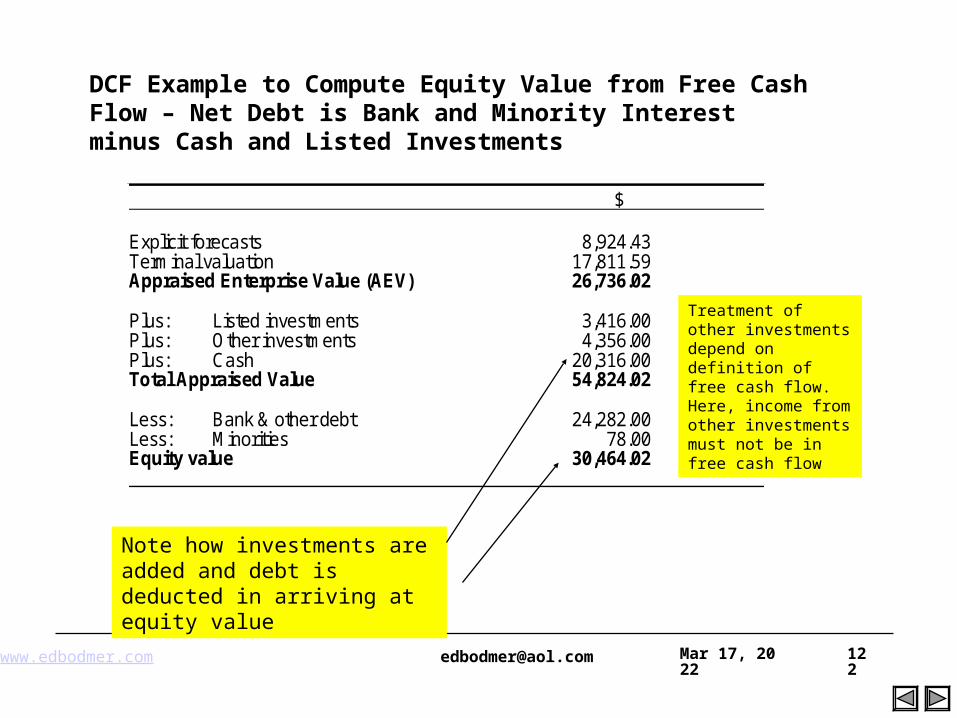
$ Explicit forecasts 8,924.43 Terminal valuation 17,811.59 Appraised Enterprise Value (AEV) 26,736.02 Plus: Listed investments 3,416.00 Plus: Other investments 4,356.00 Plus: Cash 20,316.00 Total Appraised Value 54,824.02 Less: Bank & other debt 24,282.00 Less: Minorities 78.00 Equity value 30,464.02
DCF Example to Compute Equity Value from Free Cash Flow – Net Debt is Bank and Minority Interest minus Cash and Listed Investments
Note how investments are added and debt is deducted in arriving at equity value
Treatment of other investments depend on definition of free cash flow. Here, income from other investments must not be in free cash flow
www.edbodmer.com [email protected] Apr 19, 2023 123
Example of DCF
• Lehman Brothers and Evercore calculated per share equity values by:
first determining a range of enterprise values of BellSouth by
adding the present values of the after-tax unlevered free cash flows and
terminal values for each EBITDA terminal multiple and discount rate scenario
then subtracting from the enterprise values the net debt (which is total debt minus cash) and
dividing those amounts by the number of fully diluted shares of BellSouth.
www.edbodmer.com [email protected] Apr 19, 2023 124
Discounted Cash Flow Example
• JPMorgan conducted a discounted cash flow analysis to determine a range of estimated equity values per diluted share for Exelon common stock.
• JPMorgan calculated the present value of the Exelon cash flow streams from 2005 through 2009, assuming it continued to operate as a stand-alone entity, based on financial projections for 2005 through 2007 and extensions of those projections from 2008 through 2009 in each case provided by Exelon's management.
• JPMorgan also calculated an implied range of terminal values for Exelon at the end of 2009 by applying a range of multiples of 8.0x to 9.0x to Exelon's 2009 EBITDA assumption.
• The cash flow streams and the range of terminal values were then discounted to present values using a range of discount rates from 5.25% to 5.75%, which was based on Exelon's estimated weighted average cost of capital, to determine a discounted cash flow value range.
• The value of Exelon's common stock was derived from the discounted cash flow value range by subtracting Exelon's debt and adding Exelon's cash and cash equivalents outstanding as of December 31, 2004.
www.edbodmer.com [email protected] Apr 19, 2023 125
Example of Discounted Cash Flow Analysis
• For the Exelon discounted cash flow analysis, Lehman Brothers calculated terminal values by applying a range of terminal multiples to assumed 2009 EBITDA of 7.72x to 8.72x. This range was based on the firm value to 2004 estimated EBITDA multiple range derived in the comparable companies analysis. The cash flow streams and terminal values were discounted to present values using a range of discount rates of 5.43% to 6.43%. From this analysis, Lehman Brothers calculated a range of implied equity values per share of Exelon common stock.
• PSE&G: For PSEG's regulated utility subsidiary, Morgan Stanley calculated a range of terminal values at the end of the projection period by applying a multiple to PSE&G's projected 2009 earnings and then adding back the projected debt and preferred stock amounts in 2009. The price to earnings multiple range used was 14.0x to 15.0x and the weighted average cost of capital was 5.5% to 6.0%.
www.edbodmer.com [email protected] Apr 19, 2023 126
DCF Model Issues and Problems
• The basic structure of a DCF model is simple; more complex issues include:
How to precisely discount including mid-year cash flows, terminal values, and transaction periods
How to make terminal growth consistent with multiples and inflation in the WACC
How to account for deferred taxes, net operating loss, unfunded pension plans, derivatives, stock option plans, minority interest, asset retirement obligations and other liabilities
How to account for high cost debt that has been issued by the company being valued
www.edbodmer.com [email protected] Apr 19, 2023 127
Example of Bad DCF
• In valuing a bank in Tanzania:
The WACC used included country premium that produced a WACC of 22%
The assets of the bank are not loans, but are government securities
The terminal growth rate was 2%
To make the valuation consistent with multiples in Kenya and Nigeria, liquidity and other discounts that reduced the PE multiple from about 20 to about 8.
www.edbodmer.com [email protected] Apr 19, 2023 128
• Discounted cash flow models have assumptions about net capital expenditures and growth that are strongly linked. When capital expenditures change, then the growth rate should change. There are two types of errors that show up in these valuations.
First, high growth firms with high net capital expenditures are assumed to keep reinvesting at current rates, even as growth drops off. Not surprisingly, these firms are not valued very highly in these models.
Second, the net capital expenditures are reduced to zero in stable growth, even as the firm is assumed to grow at some rate forever. Here, the valuations tend to be too high.Avoid errors and make the assumptions about reinvestment a function of the growth and the return on capital. As growth changes, the reinvestment rate must change.
Common Errors in Discounted Cash Flow Model
www.edbodmer.com [email protected] Apr 19, 2023 129
Three Issues that Can Add Complexity
• Deferred Taxes
• Employee Stock Options and Diluted Shares
• Minority Interest
• Derivatives Valued on Balance Sheet
• Asset Retirement Obligations
• High Interest Rate Debt
• Over-funded or Under-Funded Defined Pension Obligations
• The key is to understand how these items affect the value in theory and be able to work through examples
www.edbodmer.com [email protected] Apr 19, 2023 130
Deferred Tax
• There are two ways to consider deferred tax:
Option 1:
Ignore deferred tax in the calculation of free cash flow and either add or subtract deferred tax assets or liabilities
Option 2:
Model deferred tax as part of free cash flows and explicitly model the net operating loss
Option 1 has problems
Models future liability even though the future capital expenditures create new cash flows
Does not consider the timing of NOL
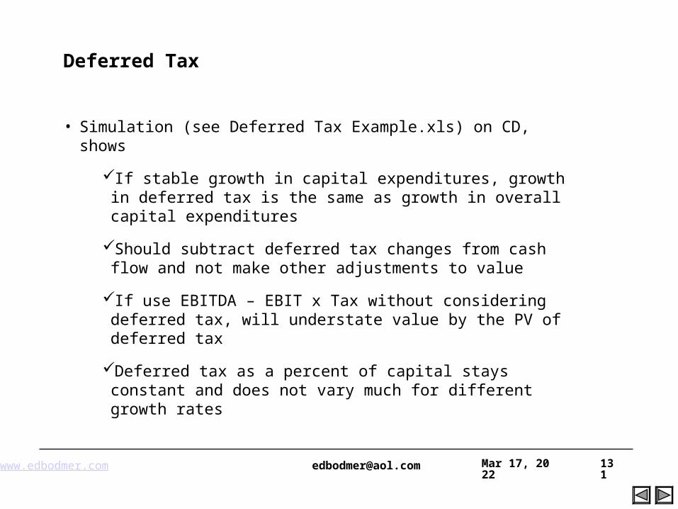
www.edbodmer.com [email protected] Apr 19, 2023 131
Deferred Tax
• Simulation (see Deferred Tax Example.xls) on CD, shows
If stable growth in capital expenditures, growth in deferred tax is the same as growth in overall capital expenditures
Should subtract deferred tax changes from cash flow and not make other adjustments to value
If use EBITDA – EBIT x Tax without considering deferred tax, will understate value by the PV of deferred tax
Deferred tax as a percent of capital stays constant and does not vary much for different growth rates
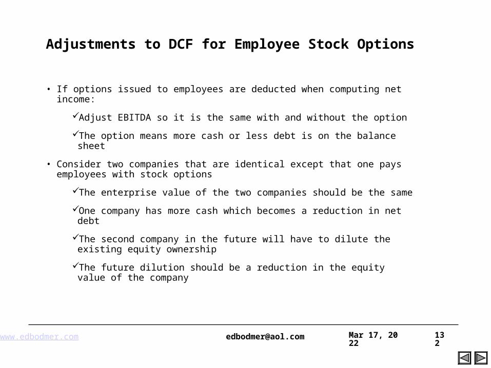
www.edbodmer.com [email protected] Apr 19, 2023 132
Adjustments to DCF for Employee Stock Options
• If options issued to employees are deducted when computing net income:
Adjust EBITDA so it is the same with and without the option
The option means more cash or less debt is on the balance sheet
• Consider two companies that are identical except that one pays employees with stock options
The enterprise value of the two companies should be the same
One company has more cash which becomes a reduction in net debt
The second company in the future will have to dilute the existing equity ownership
The future dilution should be a reduction in the equity value of the company
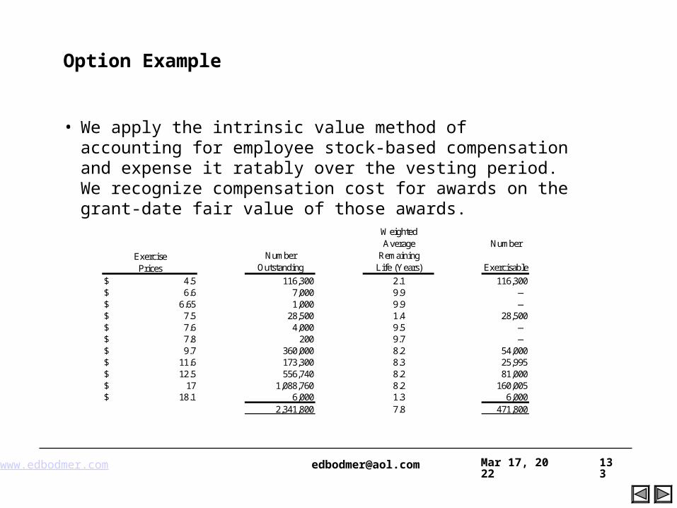
www.edbodmer.com [email protected] Apr 19, 2023 133
Option Example
• We apply the intrinsic value method of accounting for employee stock-based compensation and expense it ratably over the vesting period. We recognize compensation cost for awards on the grant-date fair value of those awards.
Number Outstanding
Weighted Average
Remaining Life (Years)
Number
Exercisable
$ 4.5 116,300 2.1 116,300$ 6.6 7,000 9.9 —$ 6.65 1,000 9.9 —$ 7.5 28,500 1.4 28,500$ 7.6 4,000 9.5 —$ 7.8 200 9.7 —$ 9.7 360,000 8.2 54,000$ 11.6 173,300 8.3 25,995$ 12.5 556,740 8.2 81,000$ 17 1,088,760 8.2 160,005$ 18.1 6,000 1.3 6,000
2,341,800 7.8 471,800
Exercise Prices
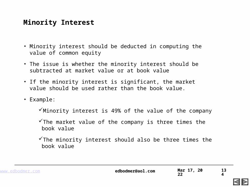
www.edbodmer.com [email protected] Apr 19, 2023 134
Minority Interest
• Minority interest should be deducted in computing the value of common equity
• The issue is whether the minority interest should be subtracted at market value or at book value
• If the minority interest is significant, the market value should be used rather than the book value.
• Example:
Minority interest is 49% of the value of the company
The market value of the company is three times the book value
The minority interest should also be three times the book value
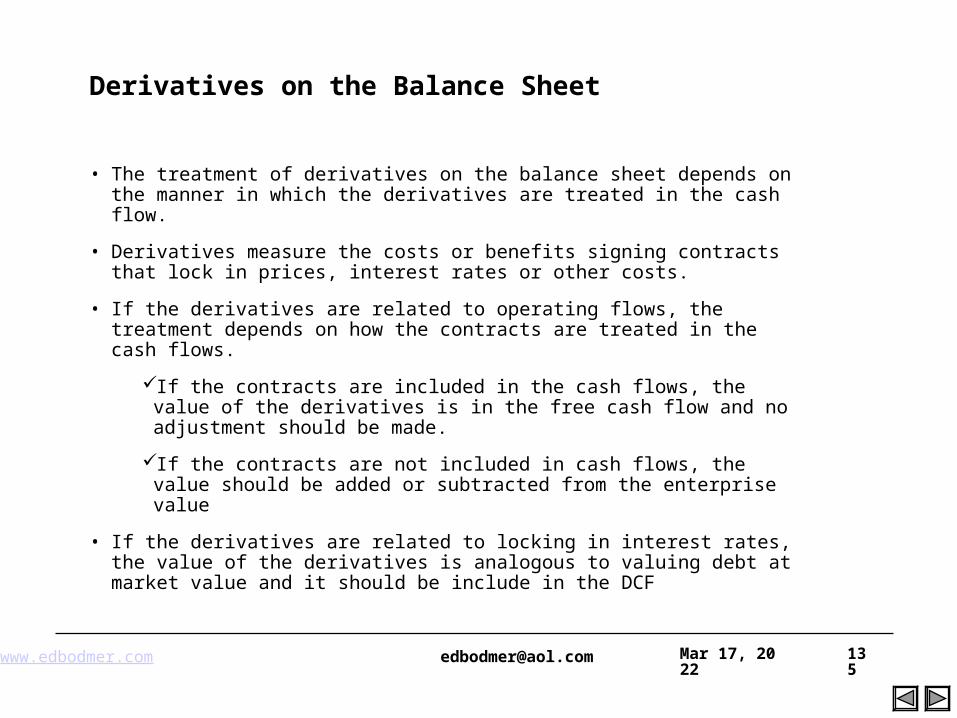
www.edbodmer.com [email protected] Apr 19, 2023 135
Derivatives on the Balance Sheet
• The treatment of derivatives on the balance sheet depends on the manner in which the derivatives are treated in the cash flow.
• Derivatives measure the costs or benefits signing contracts that lock in prices, interest rates or other costs.
• If the derivatives are related to operating flows, the treatment depends on how the contracts are treated in the cash flows.
If the contracts are included in the cash flows, the value of the derivatives is in the free cash flow and no adjustment should be made.
If the contracts are not included in cash flows, the value should be added or subtracted from the enterprise value
• If the derivatives are related to locking in interest rates, the value of the derivatives is analogous to valuing debt at market value and it should be include in the DCF
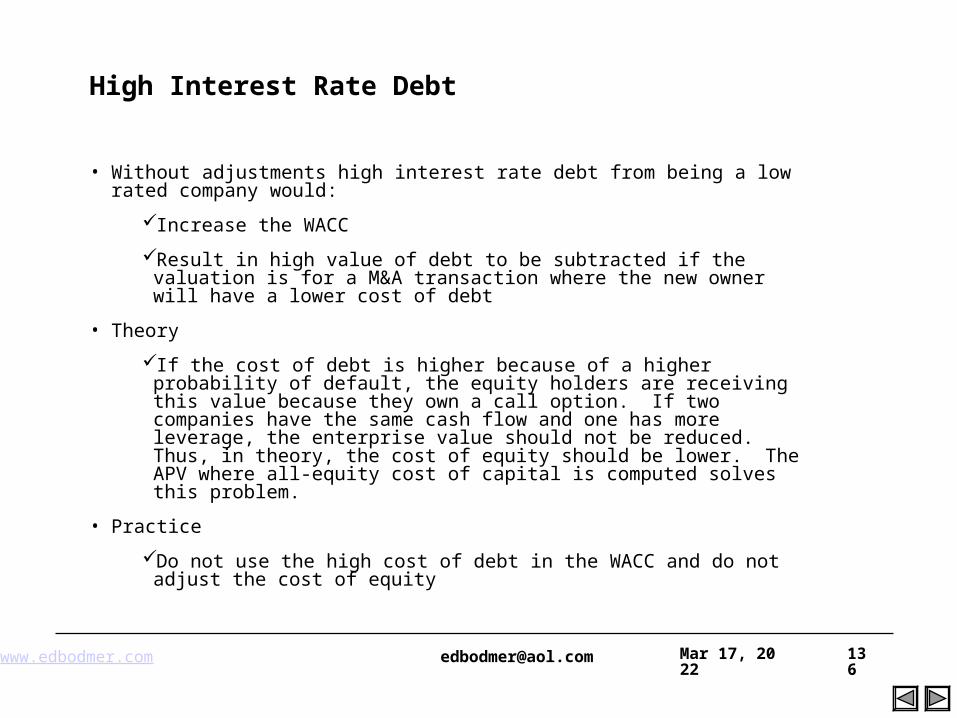
www.edbodmer.com [email protected] Apr 19, 2023 136
High Interest Rate Debt
• Without adjustments high interest rate debt from being a low rated company would:
Increase the WACC
Result in high value of debt to be subtracted if the valuation is for a M&A transaction where the new owner will have a lower cost of debt
• Theory
If the cost of debt is higher because of a higher probability of default, the equity holders are receiving this value because they own a call option. If two companies have the same cash flow and one has more leverage, the enterprise value should not be reduced. Thus, in theory, the cost of equity should be lower. The APV where all-equity cost of capital is computed solves this problem.
• Practice
Do not use the high cost of debt in the WACC and do not adjust the cost of equity
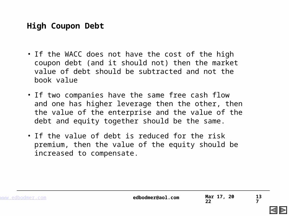
www.edbodmer.com [email protected] Apr 19, 2023 137
High Coupon Debt
• If the WACC does not have the cost of the high coupon debt (and it should not) then the market value of debt should be subtracted and not the book value
• If two companies have the same free cash flow and one has higher leverage then the other, then the value of the enterprise and the value of the debt and equity together should be the same.
• If the value of debt is reduced for the risk premium, then the value of the equity should be increased to compensate.
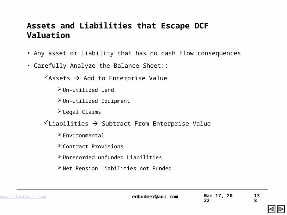
www.edbodmer.com [email protected] Apr 19, 2023 138
Assets and Liabilities that Escape DCF Valuation
• Any asset or liability that has no cash flow consequences
• Carefully Analyze the Balance Sheet::
Assets Add to Enterprise Value
Un-utilized Land
Un-utilized Equipment
Legal Claims
Liabilities Subtract From Enterprise Value
Environmental
Contract Provisions
Unrecorded unfunded Liabilities
Net Pension Liabilities not Funded
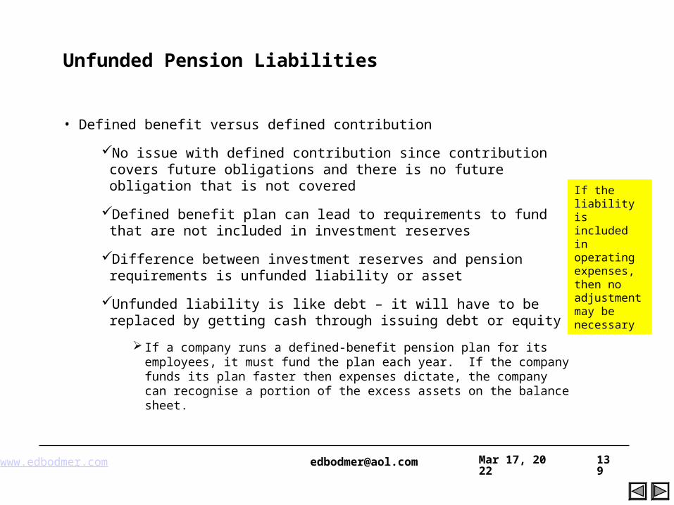
www.edbodmer.com [email protected] Apr 19, 2023 139
Unfunded Pension Liabilities
• Defined benefit versus defined contribution
No issue with defined contribution since contribution covers future obligations and there is no future obligation that is not covered
Defined benefit plan can lead to requirements to fund that are not included in investment reserves
Difference between investment reserves and pension requirements is unfunded liability or asset
Unfunded liability is like debt – it will have to be replaced by getting cash through issuing debt or equity
If a company runs a defined-benefit pension plan for its employees, it must fund the plan each year. If the company funds its plan faster then expenses dictate, the company can recognise a portion of the excess assets on the balance sheet.
If the liability is included in operating expenses, then no adjustment may be necessary
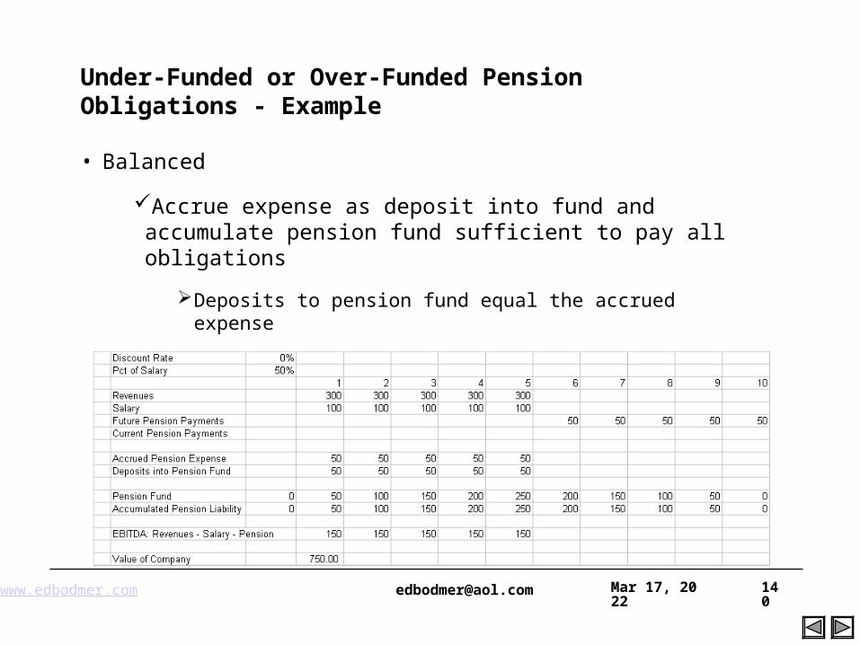
www.edbodmer.com [email protected] Apr 19, 2023 140
Under-Funded or Over-Funded Pension Obligations - Example
• Balanced
Accrue expense as deposit into fund and accumulate pension fund sufficient to pay all obligations
Deposits to pension fund equal the accrued expense
Pension liability for future payments equals pension fund
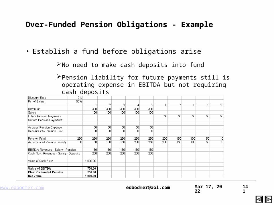
www.edbodmer.com [email protected] Apr 19, 2023 141
Over-Funded Pension Obligations - Example
• Establish a fund before obligations arise
No need to make cash deposits into fund
Pension liability for future payments still is operating expense in EBITDA but not requiring cash deposits
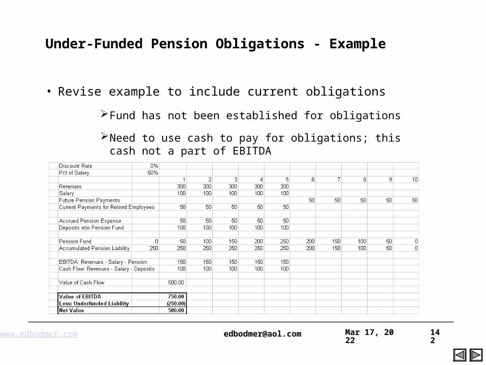
www.edbodmer.com [email protected] Apr 19, 2023 142
Under-Funded Pension Obligations - Example
• Revise example to include current obligations
Fund has not been established for obligations
Need to use cash to pay for obligations; this cash not a part of EBITDA
ValuationApr 19, 2023143
Terminal Value
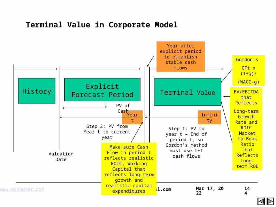
www.edbodmer.com [email protected] Apr 19, 2023 144
Terminal Value in Corporate Model
Explicit Forecast Period Terminal Value
Year t Infinity
Step 1: PV to year t – End of period t, so Gordon’s method must use t+1 cash
flows
Step 2: PV from Year t to current year
PV of Cash
Valuation Date
History
Gordon’s
CFt x (1+g)/
(WACC-g)
EV/EBITDA that Reflects
Long-term Growth Rate
and ROIC
Market to Book Ratio
that Reflects
Long-term ROE
Make sure Cash Flow in period t reflects realistic ROIC, Working Capital that reflects long-term growth and realistic capital expenditures
Year after explicit period to establish stable cash flows
www.edbodmer.com [email protected] Apr 19, 2023 145
Estimating Continuing Value
• Continuing value is important aspect of valuation
• In actual valuations compiled by McKinsey, the terminal value is – 56% to 125% of valuation
• High terminal values are reasonable if cash flow in early years is offset by outflows for capital spending that should generate higher cash flows in later years
The terminal value should reflect cash flow and earnings that is at the middle of the business cycle, or in the case of commodities, where prices reflect long-run marginal production cost, or in the case of high growth companies, when the market is saturated
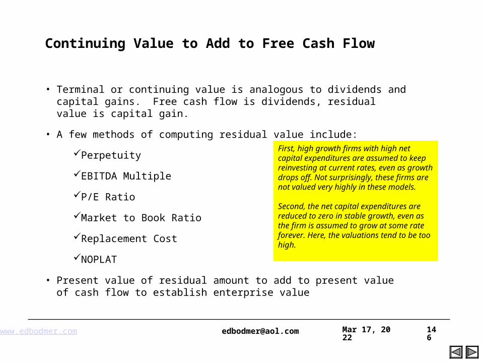
www.edbodmer.com [email protected] Apr 19, 2023 146
• Terminal or continuing value is analogous to dividends and capital gains. Free cash flow is dividends, residual value is capital gain.
• A few methods of computing residual value include:
Perpetuity
EBITDA Multiple
P/E Ratio
Market to Book Ratio
Replacement Cost
NOPLAT
• Present value of residual amount to add to present value of cash flow to establish enterprise value
Continuing Value to Add to Free Cash Flow
First, high growth firms with high net capital expenditures are assumed to keep reinvesting at current rates, even as growth drops off. Not surprisingly, these firms are not valued very highly in these models.
Second, the net capital expenditures are reduced to zero in stable growth, even as the firm is assumed to grow at some rate forever. Here, the valuations tend to be too high.
www.edbodmer.com [email protected] Apr 19, 2023 147
Capital Expenditures and Depreciation in Terminal Period
• Cash Flow can not be maintained if a company does not make investments that support the cash flow – the cash flow may be the result of earlier investments.
• Some simply set the capital expenditures equal to depreciation.
This is not correct if a company grows and experiences inflation.
The long-term stable relationship depends on the growth rate, and the depreciation rate.
With a higher growth rate and a longer depreciation life, the stable rate of Capital Expenditures/Depreciaiton increases.
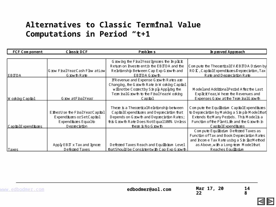
www.edbodmer.com [email protected] Apr 19, 2023 148
Alternatives to Classic Terminal Value Computations in Period “t+1”
FCF Component Classic DCF Problems Improved Approach
EBITDAGrow Final Year Cash Flow at Low
Growth Rate
Growing the Final Year Ignores the Implicit Return on Investment in the EBITDA and the Relationship Between Cap Exp Growth and
EBITDA Growth
Compute the Theoretical EV/EBITDA Driven by ROIC, Capital Expenditures/Depreciation, Tax
Rate and Depreciation Rate
Working Capital Grow at Final Year
If Revenue and Expense Growth Rates are Changing, the Growth Rate in Working Capital
will not be Correct by Simply Applying the Terminal Growth to the Final Year Working
Capital
Model and Additional Period After the Last Explicit Year, Where the Revenues and Expenses Grow at the Terminal Growth
Capital Expenditures
Either Use the Final Year Capital Expenditures or Set Capital
Expenditures Equal to Depreciation
There is a Theoretical Relationship between Capital Expenditures and Depreciation that
Depends on Growth and Depreciation Rates; this Growth Rate Does Not Equal 100% Unless
there is No Growth
Compute the Equilibrium Capital Expenditures to Depreciation by Making a Simple Model that
Extends for Many Periods. This Model is a Function of the Plant Life and the Growth in
Capital Expenditures
TaxesApply EBIT x Tax and Ignore
Deferred TaxesDeferred Taxes Reach and Equilibirum Level
that Should be Consistent with Cap Exp Growth
Compute Equilibrium Deferred Taxes as Function of Tax and Book Depreciation Rates and Income Tax Rate using a Similar Method
as Above, with a Long-term Model that Reaches Equilibrium
www.edbodmer.com [email protected] Apr 19, 2023 149
Some Terminal Value Issues
• Should you grow from a company that is already earning a high ROIC (is the ROIC sustainable)
• Should the capital expenditures in the last year be equal to the depreciation expense (if not, what should be the ratio of capital expenditures to depreciation).
• Should deferred taxes be included in the terminal year (how should the deferred taxes correspond to the depreciation assumptions)
• If multiples are used rather than a perpetuity formula, should the multiples be adjusted for prospective growth or returns
• How long should a fade period be in achieving the long-term growth
www.edbodmer.com [email protected] Apr 19, 2023 150
Formulas for Continuing Value
• A common method for computing cash flow is using the final cash flow in the corporate model and assuming the company is sold at the end of the
Perpetuity Value at beginning of final year = FCF/WACC
Perpetuity Adjusted for Growth = FCF(1+g)/(WACC - g)
Perpetuity using investment returns =
NOPLAT x (1-g/ROIC)/(WACC - g)
• Once the Perpetuity Value is established for in the last year, it must be discounted to the current value:
Current Perpetuity Value = PV(Perpetuity Value that occurs at beginning of final year)
• NPV in excel assumes flows occur at the end of the year. Adjustments can be made to assume that flows occur in the middle of the year.
In this case, the discounting of the residual is different from discounting of the individual cash flows
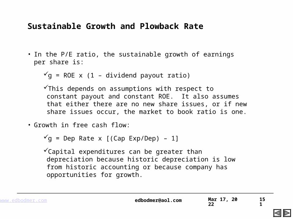
www.edbodmer.com [email protected] Apr 19, 2023 151
Sustainable Growth and Plowback Rate
• In the P/E ratio, the sustainable growth of earnings per share is:
g = ROE x (1 – dividend payout ratio)
This depends on assumptions with respect to constant payout and constant ROE. It also assumes that either there are no new share issues, or if new share issues occur, the market to book ratio is one.
• Growth in free cash flow:
g = Dep Rate x [(Cap Exp/Dep) – 1]
Capital expenditures can be greater than depreciation because historic depreciation is low from historic accounting or because company has opportunities for growth.
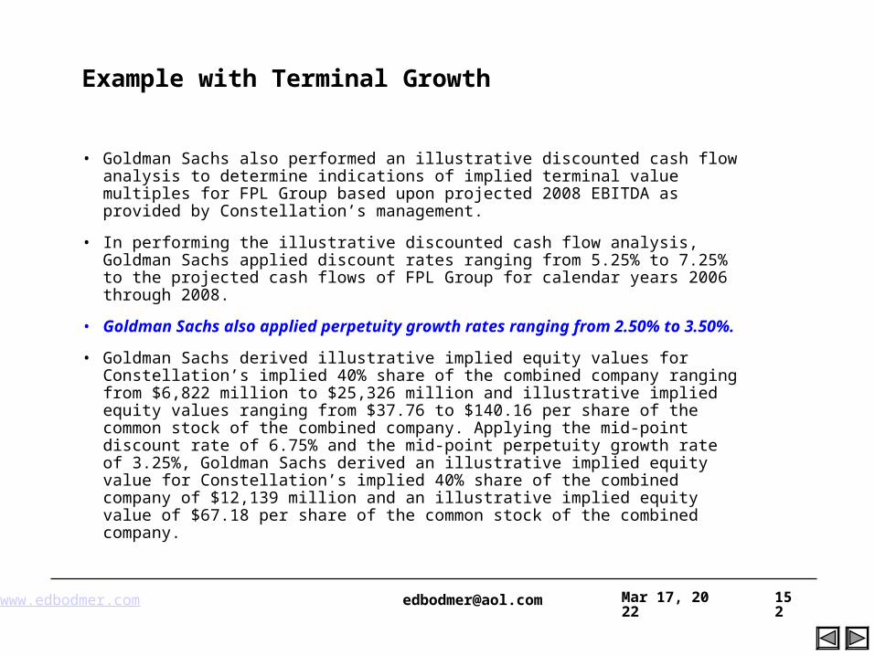
www.edbodmer.com [email protected] Apr 19, 2023 152
Example with Terminal Growth
• Goldman Sachs also performed an illustrative discounted cash flow analysis to determine indications of implied terminal value multiples for FPL Group based upon projected 2008 EBITDA as provided by Constellation’s management.
• In performing the illustrative discounted cash flow analysis, Goldman Sachs applied discount rates ranging from 5.25% to 7.25% to the projected cash flows of FPL Group for calendar years 2006 through 2008.
• Goldman Sachs also applied perpetuity growth rates ranging from 2.50% to 3.50%.
• Goldman Sachs derived illustrative implied equity values for Constellation’s implied 40% share of the combined company ranging from $6,822 million to $25,326 million and illustrative implied equity values ranging from $37.76 to $140.16 per share of the common stock of the combined company. Applying the mid-point discount rate of 6.75% and the mid-point perpetuity growth rate of 3.25%, Goldman Sachs derived an illustrative implied equity value for Constellation’s implied 40% share of the combined company of $12,139 million and an illustrative implied equity value of $67.18 per share of the common stock of the combined company.
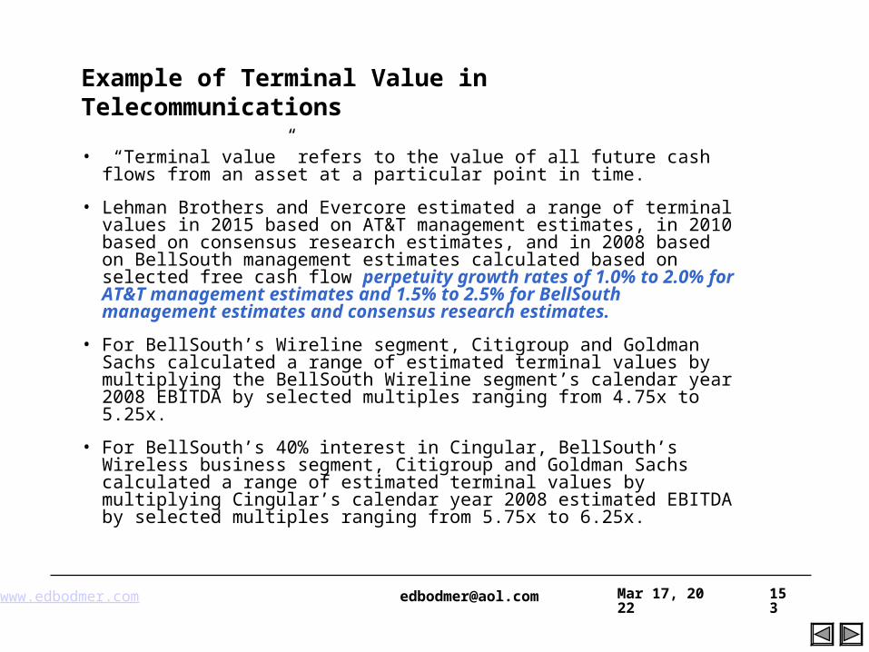
www.edbodmer.com [email protected] Apr 19, 2023 153
Example of Terminal Value in Telecommunications
• “Terminal value” refers to the value of all future cash flows from an asset at a particular point in time.
• Lehman Brothers and Evercore estimated a range of terminal values in 2015 based on AT&T management estimates, in 2010 based on consensus research estimates, and in 2008 based on BellSouth management estimates calculated based on selected free cash flow perpetuity growth rates of 1.0% to 2.0% for AT&T management estimates and 1.5% to 2.5% for BellSouth management estimates and consensus research estimates.
• For BellSouth’s Wireline segment, Citigroup and Goldman Sachs calculated a range of estimated terminal values by multiplying the BellSouth Wireline segment’s calendar year 2008 EBITDA by selected multiples ranging from 4.75x to 5.25x.
• For BellSouth’s 40% interest in Cingular, BellSouth’s Wireless business segment, Citigroup and Goldman Sachs calculated a range of estimated terminal values by multiplying Cingular’s calendar year 2008 estimated EBITDA by selected multiples ranging from 5.75x to 6.25x.
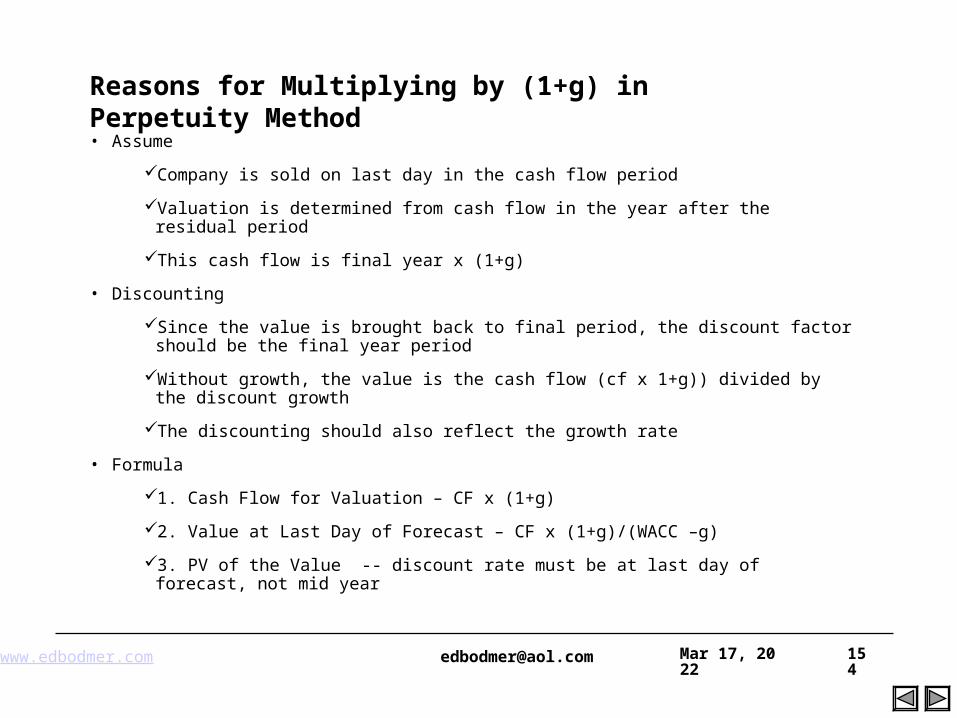
www.edbodmer.com [email protected] Apr 19, 2023 154
Reasons for Multiplying by (1+g) in Perpetuity Method
• Assume
Company is sold on last day in the cash flow period
Valuation is determined from cash flow in the year after the residual period
This cash flow is final year x (1+g)
• Discounting
Since the value is brought back to final period, the discount factor should be the final year period
Without growth, the value is the cash flow (cf x 1+g)) divided by the discount growth
The discounting should also reflect the growth rate
• Formula
1. Cash Flow for Valuation – CF x (1+g)
2. Value at Last Day of Forecast – CF x (1+g)/(WACC –g)
3. PV of the Value -- discount rate must be at last day of forecast, not mid year
www.edbodmer.com [email protected] Apr 19, 2023 155
Problems with Use of Multiples and Growth Rates in DCF
• Multiples can cause problems
Sustainable growth once stable period has been reached is probably less than the growth used in the explicit forecast period. This means that the multiple should be less as well.
The multiples for evaluating a merger transaction may include synergies and other current market items. The use of similar multiples in terminal value is highly inappropriate.
• Constant growth rates can also cause problems
Using FCF x (1+g)/(k-g) requires the assumption that growth is constant forever, and that the cost of capital will not change over time.
www.edbodmer.com [email protected] Apr 19, 2023 156
Continuing Cash Flow from NOPLAT and ROIC
• Using a multiple of NOPLAT has a couple of advantages
It is not distorted by large of small capital expenditures
Continuing value directly relates to assumptions about ROIC
For companies with low leverage, the NOPLAT multiplier is similar to the P/E ratio
• Formulas for Computing Continuing Value with NOPLAT
Free Cash = NOPLAT – Capital Expenditure + Depreciation
Free Cash = ROIC x Investment – Capital Expenditure + Depreciation
The equation becomes:
Free Cash = (1-Real Growth/Real ROIC) x NOPLAT
In this formulation
G = ROIC x Plowback Rate
Similar to ROE x Retention Rate
www.edbodmer.com [email protected] Apr 19, 2023 157
Drivers in Terminal Value
• Rather than using growth from final year, use value drivers:
Return on Invested Capital
WACC
Capital Expenditures to Depreciation
Natural growth from inflation
Real growth
• Formula for Sustainable Growth
Cap Exp/Investment – Depreciation/Investment
Cap Exp/Depreciation x Depreciation – Depreciation
• Implied EV/EBITDA can be established
www.edbodmer.com [email protected] Apr 19, 2023 158
Depreciation and Capital Expenditures in Terminal Cash Flow
• Some assume that capital expenditures equal depreciation in the final period
This would make sense if:
No past inflation
No past growth
To replace assets will have to pay current costs rather than historic costs that were affected by inflation.
If the company has grown, the stable cash flows will reflect current state of the company.
• Address with simple simulations to derive equilibrium level of capital expenditures relative to depreciation
www.edbodmer.com [email protected] Apr 19, 2023 159
Detailed Discounting Issues
• In excel, the NPV formula assumes that cash flows occur at the end of the year.
• It is more reasonable to assume that cash flows occur in the middle of the year.
• You can use discount factors that use mid-year discounting
• If the last year cash flow occurs at the middle of the year and it is assumed that the company is sold at the end of the last year, then you should use (1+g)^1.5 rather than (1+g) in discounting
• If you use XNPV it is equivalent to computing a daily discount rate with the formula (1+r)^(1/365)-1 and then using the number of days in the discounting process
ValuationApr 19, 2023160
Valuation from Projected EPS and Dividend per Share
www.edbodmer.com [email protected] Apr 19, 2023 161
Valuation from Projected Earnings and Dividends
• Earnings Valuation
PV of EPS over forecast horizon discounted at the equity discount rate
Add the present value of the perpetuity EPS value reflecting the growth rate
• Dividend Valuation
PV of Dividend per share over the forecast horizon
Add present value of book value per share rather than perpetuity of earnings because book value grows when dividends are not paid
Can multiply the book value per share by market to book multiple
www.edbodmer.com [email protected] Apr 19, 2023 162
Price Earnings and Gordon Model
Gordon Dividend Discount Model.
P = D1/(K – G)
P = the "correct" share price
D = dividend payment for the next period (recall from discounting exercise that the next period must be used)
K = Required rate of return (based largely on market interest rates a adjusted for equity risk)
G = anticipate rate of dividend growth
The model can be used to compute the cost of capital where:
R = D/P + G
Problem: D is not EPS and G is affected by payout ratio
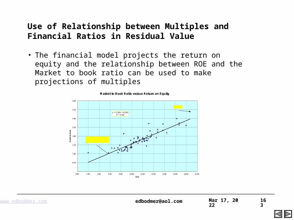
www.edbodmer.com [email protected] Apr 19, 2023 163
Use of Relationship between Multiples and Financial Ratios in Residual Value
• The financial model projects the return on equity and the relationship between ROE and the Market to book ratio can be used to make projections of multiples
Market to Book Ratio versus Return on Equity
y = 13.102x + 0.2595
R2 = 0.786
-
0.50
1.00
1.50
2.00
2.50
3.00
3.50
4.00
0.0% 2.0% 4.0% 6.0% 8.0% 10.0% 12.0% 14.0% 16.0% 18.0% 20.0% 22.0%
ROE
Ma
rke
t to
Bo
ok
Return on equity associated with a market to book ratio of 1.0
Exelon
ValuationApr 19, 2023164
Reference: Selected Valuation Issues
www.edbodmer.com [email protected] Apr 19, 2023 165
• 1. How do you choose between firm and equity valuation (DCF valuation versus Earnings Growth)
• Done right, firm and equity valuation should yield the same values for the equity with consistent assumptions. Choosing between firm (DCF) and equity valuation (PE x EPS forecasts) boils down to the pragmatic issue of ease.
• For banks, firm valuation does not work because small differences in WACC can have dramatic effects on valuation while and if the market value of debt differs from the book value, firm value can cause distortions.
Valuation Issues
www.edbodmer.com [email protected] Apr 19, 2023 166
• From the perspective of convenience, it is often easier to estimate equity than the DCF, especially when leverage is changing significantly over time (for example, in project finance and in leveraged buyouts where equity IRR is used).
• Equity value measures a real cash flow to owners, rather than an abstraction (free cash flows to the firm exist only on paper).
• Free cash flow is affected to a large extent by capital expenditures which can cause problems.
• Equity cash fllow brings to light potential cash shortfalls (and the likelihood of bankruptcy) much more directly
Firm versus Equity Valuation
www.edbodmer.com [email protected] Apr 19, 2023 167
• While there are many who use historical (past) growth as a measure of expected growth, or choose to trust analysts (with their projections), try using fundamentals.
• Think about the two factors that determine growth - the firm's reinvestment policy and its rate of return.
For expected growth in earnings = Retention Ratio * ROE, where Retention Ratio is 1 – Dividend Payout
For expected growth in EBIT = Reinvestment Rate * ROC, where reinvestment rate is Cap Exp/Depreciation
Measurement of Expected Growth Rate
www.edbodmer.com [email protected] Apr 19, 2023 168
• Terminal value refers to the value of the firm (or equity) at the end of the high growth period. Estimate terminal value, with DCF, by assuming a stable growth rate that the firm can sustain forever. If we make this assumption, the terminal value becomes:
• Terminal Value in year n = Cash Flow in year n+1 / (r - g)
• This approach requires the assumption that growth is constant forever, and that the cost of capital will not change over time.
Estimation of Terminal Value
www.edbodmer.com [email protected] Apr 19, 2023 169
• In some discounted cash flow valuations, the terminal value is estimated using a multiple, usually of earnings. In an equity valuation model, the exit multiple may be the PE ratio. In firm valuation models, the exit multiple is often of EBIT or EBITDA.
• Analysts who use these multiples argue that it saves them from the dangers of having to assume a stable growth rate and that it ties in much more closely with their objective of selling the firm or equity to someone else at the end of the estimation period.
• Problems arise if the PE assumes a higher growth than is sustainable after the holding period.
Exit multiple in DCF valuation
www.edbodmer.com [email protected] Apr 19, 2023 170
• On the contrary, exit multiples may introduce relative valuation into discounted cash flow valuation, and that you create a hybrid, which is neither DCF nor relative valuation. These exit multiples use the biggest single assumption made in these valuation models.
• It seems foolish to assume that current multiples will remain constant as the industry matures and changes and that investors will continue to pay high multiples, even if the fundamentals do not justify them. If there is stable growth, the P/E multiple in the terminal value should be lower.
Exit multiples and DCF valuation
www.edbodmer.com [email protected] Apr 19, 2023 171
• There are a number of reasons why a firm might have negative earnings, and the response will vary depending upon the reason:- If the earnings of a cyclical firm are depressed due to a recession, the best response is to normalize earnings by taking the average earnings over a entire business cycle.
- Normalized Net Income = Average ROE * Current Book Value of Equity- Normalized after-tax Operating Income = Average ROC * Current Book Value of Assets- Once earnings are normalized, the growth rate used should be consistent with the normalized earnings, and should reflect the real growth potential of the firm rather than the cyclical effects.
Valuation of Firms that are Losing Money
www.edbodmer.com [email protected] Apr 19, 2023 172
• - If the earnings of a firm are depressed due to a one-time charge, the best response is to estimate the earnings without the one-time charge and value the firm based upon these earnings. - If the earnings of a firm are depressed due to poor quality management, the average return on equity or capital for the industry can be used to estimate normalized earnings for the firm. The implicit assumption is that the firm will recover back to industry averages, once management has been removed.- Normalized Net Income = Industry-average ROE * Current Book Value of Equity- Normalized after-tax Operating Income = Industry-average ROC * Current Book Value of Assets
Valuation of a firm that is Losing Money
www.edbodmer.com [email protected] Apr 19, 2023 173
• - If the negative earnings over time have caused the book value to decline significantly over time, use the average operating or profit margins for the industry in conjunction with revenues to arrive at normalized earnings. Thus, a firm with negative operating income today could be assumed to converge on the normalized earnings five years from now. - If the earnings of a firm are depressed or negative because it operates in a sector which is in its early stages of its life cycle, the discounted cash flow valuation will be driven by the perception of what the operating margins and returns on equity (capital) will be when the sector matures.
• - If the equity earnings are depressed due to high leverage, the best solution is to value the firm rather than just the equity, factoring in the reduction in leverage over time.
Valuation of a firm that is losing money
www.edbodmer.com [email protected] Apr 19, 2023 174
• The valuation of a private firm is more difficult than stock in a publicly traded firm. In particular,
A. The information available on private firms will be sketchier than the information available on publicly traded firms.
B. Past financial statements, even when available, might not reflect the true earnings potential of the firm. Many private businesses understate earnings to reduce their tax liabilities, and the expenses at many private businesses often reflect the blurring of lines between private and business expenses.
Valuation of a private firms
www.edbodmer.com [email protected] Apr 19, 2023 175
• C. The owners of many private businesses are taxed on the salary they make and the dividends they take out of the business; often do not try to distinguish between the two.The limited availability of information does make the estimation of cash flows impossible; past financial statements might need to be restated to make them reflect the true earnings of the firm. Once the cash flows are estimated, the choice of a discount rate might be affected by the identity of the potential buyer of the business. If the potential buyer of the business is a publicly traded firm, the valuation should be done using the discount rates based upon market risk
Valuation of a private firm
www.edbodmer.com [email protected] Apr 19, 2023 176
EPS Measures – Establishing a reliable starting point
• Reported EPS – EPS reported by the company using generally accepted accounting principles. Therefore includes earnings from recurring and non-recurring items
• Recurring EPS – Reported EPS adjusted to exclude non-recurring items
• Fully diluted EPS – EPS adjusted to reflect dilution to existing shareholders as a result of future increases in equity shares
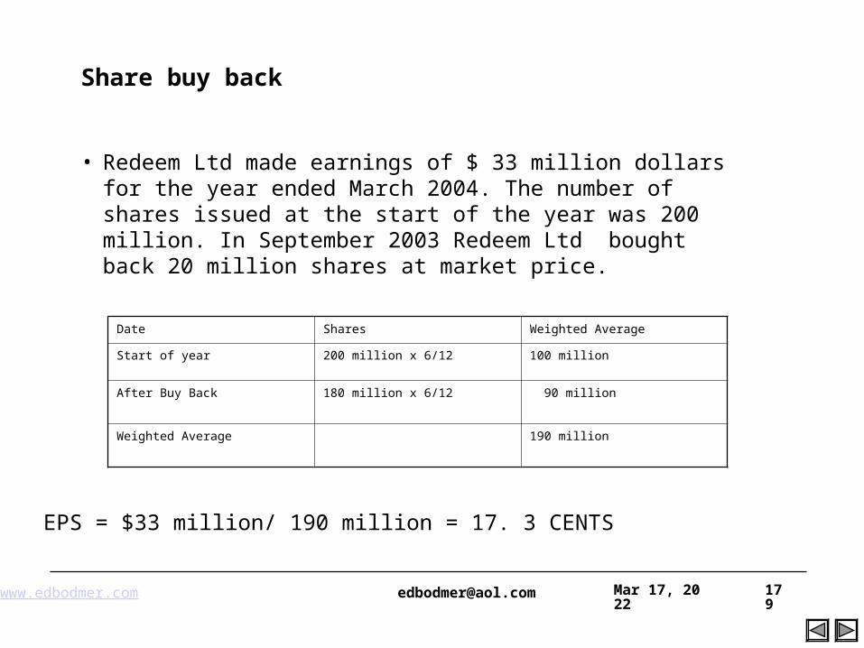
www.edbodmer.com [email protected] Apr 19, 2023 179
Date Shares Weighted Average
Start of year 200 million x 6/12 100 million
After Buy Back 180 million x 6/12 90 million
Weighted Average 190 million
EPS = $33 million/ 190 million = 17. 3 CENTS
Share buy back
• Redeem Ltd made earnings of $ 33 million dollars for the year ended March 2004. The number of shares issued at the start of the year was 200 million. In September 2003 Redeem Ltd bought back 20 million shares at market price.
www.edbodmer.com [email protected] Apr 19, 2023 180
Dilution – Factors and treatment
• Contingently issuable shares - Include shares in the calculation of basic EPS if the contingency has been met.
• Options or warrants in existence over as yet un-issued shares – Assume exercise of outstanding dilutive options and warrants
• Loan stock or preference shares convertible into equity shares in the future – Assume that instruments are converted therefore saving interest but increasing the number of shares in issue
www.edbodmer.com [email protected] Apr 19, 2023 181
Diluted Shares
• If you have agreed to give away shares to someone, then your claim to the cash flow of the company is reduced.
• In the extreme, if you have given away half of your company away, and the cash flow is the same before and after your give away, then the amount you would pay for the share must account for how much you will give away.
• In this extreme example, you should reduce the value by ½.
• This can be accomplished by using diluted shares rather than basic shares.
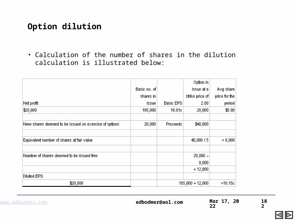
www.edbodmer.com [email protected] Apr 19, 2023 182
Option dilution
• Calculation of the number of shares in the dilution calculation is illustrated below:
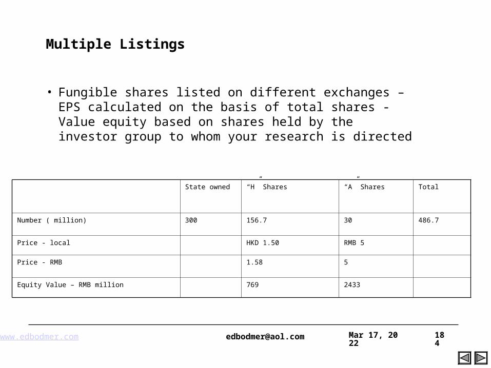
www.edbodmer.com [email protected] Apr 19, 2023 184
State owned “H” Shares “A” Shares Total
Number ( million) 300 156.7 30 486.7
Price - local HKD 1.50 RMB 5
Price - RMB 1.58 5
Equity Value – RMB million 769 2433
Multiple Listings
• Fungible shares listed on different exchanges – EPS calculated on the basis of total shares - Value equity based on shares held by the investor group to whom your research is directed
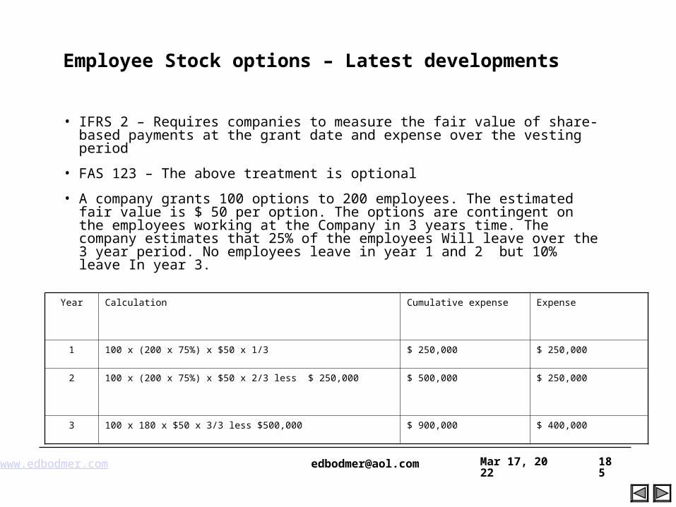
www.edbodmer.com [email protected] Apr 19, 2023 185
Year Calculation Cumulative expense Expense
1 100 x (200 x 75%) x $50 x 1/3 $ 250,000 $ 250,000
2 100 x (200 x 75%) x $50 x 2/3 less $ 250,000 $ 500,000 $ 250,000
3 100 x 180 x $50 x 3/3 less $500,000 $ 900,000 $ 400,000
Employee Stock options – Latest developments
• IFRS 2 – Requires companies to measure the fair value of share-based payments at the grant date and expense over the vesting period
• FAS 123 – The above treatment is optional
• A company grants 100 options to 200 employees. The estimated fair value is $ 50 per option. The options are contingent on the employees working at the Company in 3 years time. The company estimates that 25% of the employees Will leave over the 3 year period. No employees leave in year 1 and 2 but 10% leave In year 3.
www.edbodmer.com [email protected] Apr 19, 2023 186
Issues in the application of PEs
• Accounting Policy differences – Particularly significant for cross border comparisons where companies may follow local, international or US GAAP
• Loss making companies – No earnings therefore no PE
• Cyclical companies – PEs volatile through the cycle and therefore difficult to benchmark
• Finding a suitable benchmark – Difficult to find companies that are perfect matches in all determinants of a PE
• Growth – As discussed value and growth are not always the same
• Capital market conditions – The cost of equity will vary depending on underlying interest rate environment that is likely to be different in different countries
• Financing – The greater the gearing of a company the greater the cost of equity and therefore, all other things being equal, the lower the value and the lower the PE
www.edbodmer.com [email protected] Apr 19, 2023 187
Valuation of Subsidiary Companies in Different Countries
• How would things differ if we are valuing companies from different countries, different sectors etc.
• The basic rule is:
Cash flows should be nominal
Cash flows should be stated in the currency where the subsidiary is located
If there are multiple currencies, use the future expected spot exchange rates to translate cash flows
Cash flows should be discounted at cost of capital that reflects the interest rates where the country is located
This means that the risk free rate in the country where the subsidiary is located should be used.
Once the value is established, translate the amount to the home country at the spot exchange rate
www.edbodmer.com [email protected] Apr 19, 2023 188
Valuation of Subsidiary Companies in Different Countries
• How would things differ if we are valuing companies from different countries, different sectors etc.
Example:
Subsidiary is located in Malaysia
Parent Company is in Hong Kong
Subsidiary company sells in Malaysia and Thailand
Subsidiary company produces in Malaysia and Thailand
Exchange Rates and Interest Rates
Spot Exchange Rates
HK Dollars to Ringet Baht to Ringet
www.edbodmer.com [email protected] Apr 19, 2023 189
Valuation of Subsidiary Companies in Different Countries
• How would things differ if we are valuing companies from different countries, different sectors etc.
• Cash flows should be stated in the currency where the subsidiary is located (Malaysian Ringgit)
Compute prices and costs in Baht and Ringgit and then translate the revenues and costs in Baht to Ringgit
To convert the Baht to Ringgit, use the expected future spot Ringet/Baht exchange rates
Since, as a practical matter, forward exchange rates are not available beyond 18 months, compute future spot rates from interest rate parity
Interest rate parity means that if you invest in risk free securities of different currencies, the spot exchange rate must reflect the future values.
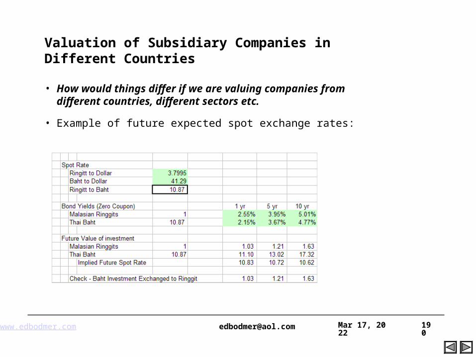
www.edbodmer.com [email protected] Apr 19, 2023 190
Valuation of Subsidiary Companies in Different Countries
• How would things differ if we are valuing companies from different countries, different sectors etc.
• Example of future expected spot exchange rates:
www.edbodmer.com [email protected] Apr 19, 2023 192
Free Cash Flow
We often talk about free cash flow, sometimes, it is challenging to assess what is "free“ cash flow or not, may wish to elaborate on that rather than just defining free cash flow in a text book term.
The basic point is to keep things consistent. If you define FCF as EBITDA without other income, then the valuation does not include other investments.
On the other hand if FCF is defined using Cash B/4 Financing that includes other income, the other investments are included in the valuation
www.edbodmer.com [email protected] Apr 19, 2023 193
In-the-money Options and Convertibles
• Can the trainer also cover dealing with in-the money options and convertibles?
• Convertibles can trade as straight debt if it is unlikely that the convertibles will be converted to common shares, or if the conversion option is in the money, it is clear that the convertibles will be switched into common shares. In this case, the ownership share of current shareholders is diluted.
• If you buy the current shares, you are not really getting the whole company because you will have to give a share of the cash flow to the convertible bondholders.
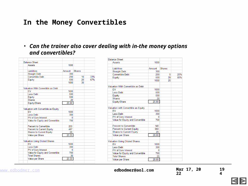
www.edbodmer.com [email protected] Apr 19, 2023 194
In the Money Convertibles
• Can the trainer also cover dealing with in-the money options and convertibles?
www.edbodmer.com [email protected] Apr 19, 2023 195
Terminal Value
Terminal value, and the use of a stable growth rate. How do you determine that, what is the rule of thumb and how do you determine which year onwards should be terminal year (i.e. how long should your forecasted period be).
On how to calculate a WACC, rather than just providing the formula of WACC, it would be useful to give instructions on where to find the market premium data, betas and what is the best method vs the most practical method.
Should we include country risk, exchange rate risks etc and how to get them.
Also there is no mentioning of cash revolver and how to calculate it.
www.edbodmer.com [email protected] Apr 19, 2023 196
LBO Valuation
• How can LBO’s be valued by making an assumption on target IRRs for the venture cap / private equity investor.
• Recall the very first simple case that was developed in the class. In this case the equity IRR was driven by the level of leverage and the structure of the debt.
• Valuation is realistically driven by the equity IRR criteria of developers and not free cash flow or WACC
• The risk metric boils down to the debt capacity of the LBO and the value of the investment depends on the debt structure.
• In this case, risk is driven by bankers outside of the company rather than the management or advisors to the company.
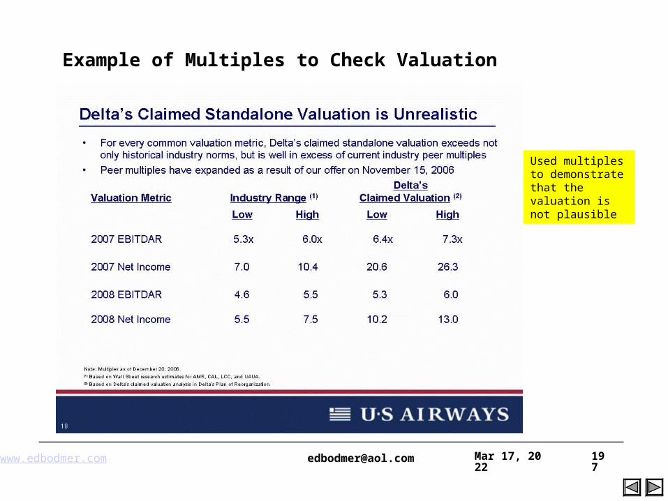
www.edbodmer.com [email protected] Apr 19, 2023 197
Example of Multiples to Check Valuation
Used multiples to demonstrate that the valuation is not plausible
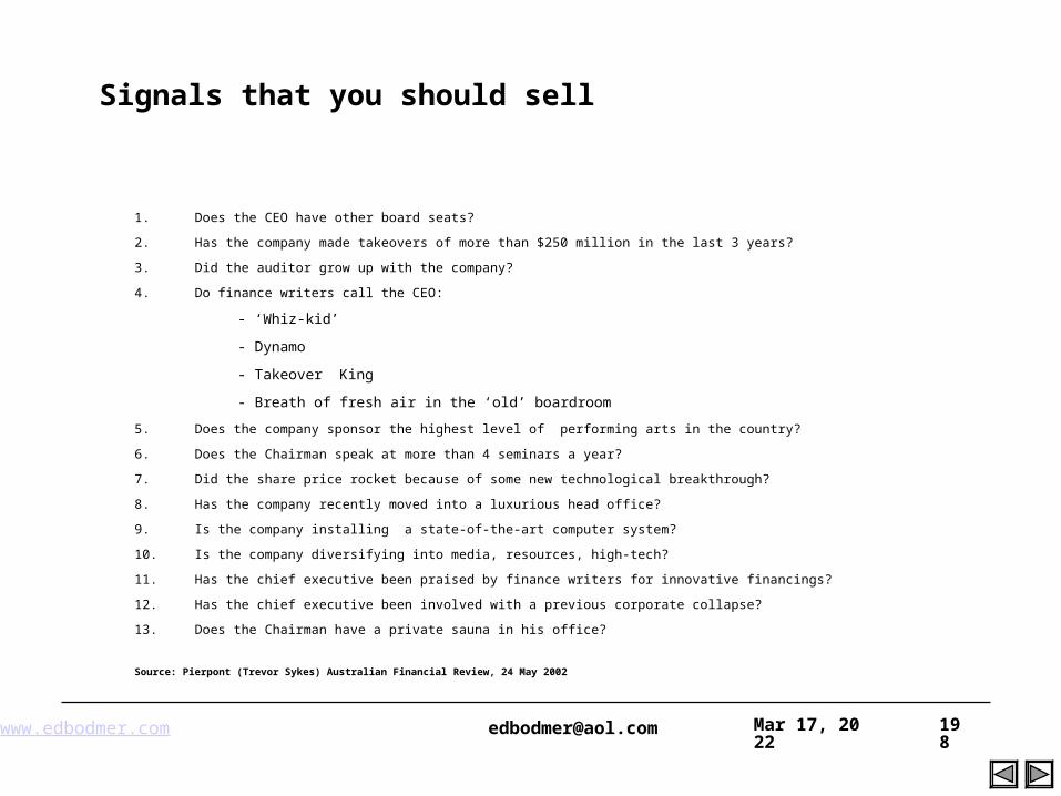
www.edbodmer.com [email protected] Apr 19, 2023 198
1. Does the CEO have other board seats?
2. Has the company made takeovers of more than $250 million in the last 3 years?
3. Did the auditor grow up with the company?
4. Do finance writers call the CEO:
- ‘Whiz-kid’
- Dynamo
- Takeover King
- Breath of fresh air in the ‘old’ boardroom
5. Does the company sponsor the highest level of performing arts in the country?
6. Does the Chairman speak at more than 4 seminars a year?
7. Did the share price rocket because of some new technological breakthrough?
8. Has the company recently moved into a luxurious head office?
9. Is the company installing a state-of-the-art computer system?
10. Is the company diversifying into media, resources, high-tech?
11. Has the chief executive been praised by finance writers for innovative financings?
12. Has the chief executive been involved with a previous corporate collapse?
13. Does the Chairman have a private sauna in his office?
Source: Pierpont (Trevor Sykes) Australian Financial Review, 24 May 2002
Signals that you should sell
www.edbodmer.com [email protected] Apr 19, 2023 199
Finance Professor
• A finance professor received a call from a large financial institution in New York, asking him to interview for a position on their scientific advisory committee. He agreed to go up and interview, knowing that such a position would be prestigious and with the extra income we would be able to purchase more consumer durables. As all of you know, interviews are a long and painful process. The interviews lasted two days and at the end of the last day the professor was interviewing with the chief executive who would ultimately be making the hiring decision. At the very end of the interview, the executive asked him, “what is 7 times 3?” The finance professor confidently responded, “22.”
• When he got home from New York his family, for once, was eagerly awaiting his return… with lists of consumer durables in their hands. “How did it go?” they asked. “Good,” he said, “except in the last interview they asked me 7x3 and I said 22.” “Ohh! Dad!!!” they cried, “it’s 21!” They threw out their lists of consumer durables, knowing he would never get the job.
• Much to his surprise he got a call 2 weeks later saying he’d gotten the position and the firm was having a reception in his honor. At the reception he found the executive and went up to him. “Do you remember our interview?” the professor asked. “Yes,” said the executive. “And do you remember when you asked me 7x3 and I said 22.” “Yes,” replied the executive, “I wrote down your answer.” “Well the correct answer is 21,” said the professor, “why did I get the job?” “Well,” said the executive, “of all the finance professors we interviewed… you were the closest.”
• The moral of the story is, if I can do this, you can do this: pricing bonds and non-American options using monte carlo simulation to replicate the results achieved explicitly using decision trees.
www.edbodmer.com [email protected] Apr 19, 2023 200
Finance Professors
• A medical doctor, an engineer, and a finance professor are at a cocktail party.
The medical doctor pompously asserts that the medical profession is the oldest profession. He cites a passage from the Bible, in Genesis where god creates man and woman. “Surely,” he says, “this was the first medical act.”
The engineer jumps in and says, “I remember a passage prior to that, which says, out of the chaos and confusion, God created the earth. Surely, this was the first act of engineering and predates the first medical act.”
“Aha!” says the finance professor, “who created the confusion?!”
www.edbodmer.com [email protected] Apr 19, 2023 201
Resources and Contacts
• My contacts
Ed Bodmer
Phone: +001-630-886-2754
E-mail: [email protected]
• Other Sources
http://pages.stern.nyu.edu/~adamodar/
www.sec.us.gov -- financial documents
www.finance.yahoo.com; www.googlefinance.com; www.valueline.com -- stock prices and financial ratios
www.standardandpoors.com; www.moodys.com – credit rating and other information
www.bondsonline.com – credit spreads