Embed Size (px)
Citation preview
TECHNISCHE UNIVERSITÄT MÜNCHEN Lehrstuhl für Finanzmathematik
Valuation of multi-dimensional derivatives in a
stochastic covariance framework
Barbara Maria Götz
Vollständiger Abdruck der von der Fakultät für Mathematik der Technischen Universität
München zur Erlangung des akademischen Grades eines
Doktors der Naturwissenschaften (Dr. rer. nat.)
genehmigten Dissertation.
Vorsitzender: Univ.-Prof. Claudia Czado, Ph.D.
Prüfer der Dissertation:
1. Univ.-Prof. Dr. Rudi Zagst
2. Prof. Dr. Marcos Escobar,
Ryerson University, Toronto/Kanada
3. Prof. Luis Seco, Ph.D.,
University of Toronto/Kanada
Die Dissertation wurde am 02.05.2011 bei der Technischen Universität München
eingereicht und durch die Fakultät für Mathematik am 21.06.2011 angenommen.

Abstract
Die Finanzkrise hat gezeigt, dass die Annahme von konstanten Kovarianzen nicht gultig
ist. Diese Arbeit beschaftigt sich daher eingehend mit der Modellierung von stochastischer
Kovarianz in den Finanzmarkten und entwickelt Techniken, die es erlauben die stochastis-
che Kovarianz als Risikotreiber in die Bewertung von Derivaten miteinzubeziehen. Wir
behandeln zwei Modelle naher, eines mit stochastischer Varianz und deterministischer
Korrelation, ein anderes mit stochastischer Varianz und Korrelation.
Fur das erste Modell konnen wir mit Hilfe von partiellen Differentialgleichungen und der
Separationsmethode semi-analytische Losungsformeln fur Barrier-Optionen herleiten. Im
zweiten Modell wenden wir Approximationstechniken der Storungstheorie an, um leicht
zu berechnende und gut konvergierende Approximationen fur Nicht-Vanillaprodukte mit
mehr als einem Basistitel zu finden.

Abstract
The financial crisis has shown that constant covariances are an assumption which is not
valid as correlations tend to increase in extreme market events. This thesis covers ap-
proaches to model stochastic covariance risk in financial markets, and develops techniques
to incorporate stochastic covariance as a risk driver in the pricing of derivatives. We treat
two models, one with stochastic variance and deterministic correlation, one with stochas-
tic variance and stochastic correlation, more closely.
For the first model we find a semi-analytic pricing formula for double-barrier options us-
ing PDEs and the method of separation. In the second model we apply the techniques
of perturbation theory to find simply computable and well converging approximations for
non-vanilla products with more than one underlying.


Acknowledgement
This research project would not have been possible without the support of many people.
I am heartily thankful to my supervisors, Prof. Escobar and Prof. Zagst. Marcos helped
me to develop my topic and to make best use of my energy and time. My research stays
in Toronto have founded the ground for my thesis and were very beneficial to me. I am
deeply grateful to Prof. Zagst, particularly for all the fruitful discussions we had about
my research ideas, for making the research stays in Toronto possible and his support to
put the finishing touches on my papers and the thesis.
Many thanks go to the Women in Math Science programme whose financial support
rendered the research stays in Toronto possible. I also would like to acknowledge the un-
derstanding of my subordinates at KPMG that I wanted to dive deeper into mathematical
theories.
I wish to express my gratitude for my husband’s and my family’s ceaseless moral support.
It is a pleasure to thank especially my father-in-law and my brother for their proofreading.

Contents
I Introduction 1
1 Introduction 3
1.1 Literature overview and purpose of the thesis . . . . . . . . . . . . . . . . 3
1.2 Summary of the results and contributions to the literature . . . . . . . . . 6
1.3 Structure of the thesis . . . . . . . . . . . . . . . . . . . . . . . . . . . . . 7
2 Mathematical preliminaries and definitions 9
2.1 Probability spaces and stochastic processes . . . . . . . . . . . . . . . . . . 9
2.2 Distribution functions and characteristic function . . . . . . . . . . . . . . 16
2.2.1 Notations . . . . . . . . . . . . . . . . . . . . . . . . . . . . . . . . 16
2.2.2 Distribution functions . . . . . . . . . . . . . . . . . . . . . . . . . 18
2.2.3 Definitions and properties of the characteristic function . . . . . . . 19
2.2.4 Characteristic function and the moments of the distribution . . . . 21
2.2.5 Uniqueness and inversion . . . . . . . . . . . . . . . . . . . . . . . . 22
2.2.6 Characteristic functions in higher dimensions . . . . . . . . . . . . . 24
2.2.7 Analytic characteristic functions . . . . . . . . . . . . . . . . . . . . 24
2.3 The Ito formula and the martingale representation theorem . . . . . . . . . 31
2.4 Diffusions and stochastic differential equations . . . . . . . . . . . . . . . . 34
2.4.1 Important examples of SDE’s in R1 . . . . . . . . . . . . . . . . . . 40
2.5 Connections between stochastic differential equations and partial differen-
tial equations . . . . . . . . . . . . . . . . . . . . . . . . . . . . . . . . . . 43
2.6 Pricing contingent claims . . . . . . . . . . . . . . . . . . . . . . . . . . . . 49
x CONTENTS
2.7 Solution of PDE . . . . . . . . . . . . . . . . . . . . . . . . . . . . . . . . . 50
II Main Part 53
3 Pricing of barrier options within stochastic covariance model 55
3.1 Introduction . . . . . . . . . . . . . . . . . . . . . . . . . . . . . . . . . . . 55
3.2 Model framework . . . . . . . . . . . . . . . . . . . . . . . . . . . . . . . . 57
3.3 Pricing of two-asset barrier options . . . . . . . . . . . . . . . . . . . . . . 58
3.4 Pricing of two-asset barrier options with Fourier techniques . . . . . . . . . 60
3.4.1 General pricing formulas for two-asset barrier options with Fourier
techniques . . . . . . . . . . . . . . . . . . . . . . . . . . . . . . . . 60
3.4.2 Properties of selected two-dimensional affine characteristic functions 73
3.4.3 Pricing of two-asset double-digital options with Fourier techniques . 78
3.4.4 Pricing of correlation barrier options with Fourier techniques . . . . 84
3.4.5 Alternative Fourier Technique . . . . . . . . . . . . . . . . . . . . . 92
3.4.6 Random correlations . . . . . . . . . . . . . . . . . . . . . . . . . . 98
3.4.7 Conclusion . . . . . . . . . . . . . . . . . . . . . . . . . . . . . . . . 98
3.5 Pricing of two-asset barrier options with PDE techniques . . . . . . . . . . 98
3.5.1 General pricing formulas for two-asset barrier options exploiting the
affine form in v . . . . . . . . . . . . . . . . . . . . . . . . . . . . . 99
3.5.2 Pricing of two-asset double-digital barrier options with PDE tech-
niques . . . . . . . . . . . . . . . . . . . . . . . . . . . . . . . . . . 108
3.5.3 Pricing of two-asset barrier correlation options with PDE techniques 111
3.5.4 Conclusion . . . . . . . . . . . . . . . . . . . . . . . . . . . . . . . . 114
3.6 Pricing certificates under issuer risk . . . . . . . . . . . . . . . . . . . . . . 115
3.6.1 Introduction . . . . . . . . . . . . . . . . . . . . . . . . . . . . . . . 115
3.6.2 The model . . . . . . . . . . . . . . . . . . . . . . . . . . . . . . . . 116
3.6.3 Pricing of certificates under issuer risk . . . . . . . . . . . . . . . . 118
3.6.4 Conclusion . . . . . . . . . . . . . . . . . . . . . . . . . . . . . . . . 137
CONTENTS xi
4 Pricing of barrier options within stochastic correlation model 139
4.1 Introduction . . . . . . . . . . . . . . . . . . . . . . . . . . . . . . . . . . . 139
4.2 Model framework . . . . . . . . . . . . . . . . . . . . . . . . . . . . . . . . 141
4.3 Data analysis for mean-reversion scales . . . . . . . . . . . . . . . . . . . . 143
4.4 Pricing of single-barrier options . . . . . . . . . . . . . . . . . . . . . . . . 150
4.5 Pricing of two-asset barrier options with perturbation theory . . . . . . . . 155
4.5.1 Approximation of Model (4.1) . . . . . . . . . . . . . . . . . . . . . 156
4.5.2 Extension of Model (4.1) . . . . . . . . . . . . . . . . . . . . . . . . 193
4.6 Conclusion . . . . . . . . . . . . . . . . . . . . . . . . . . . . . . . . . . . . 195
III Appendix 197
A Appendix for Chapter 3 199
A.1 Appendix for Section 3.4 . . . . . . . . . . . . . . . . . . . . . . . . . . . . 199
A.1.1 Transformations used for PDE . . . . . . . . . . . . . . . . . . . . . 199
A.1.2 Characteristic functions . . . . . . . . . . . . . . . . . . . . . . . . 207
A.1.3 Method of images in a half-space . . . . . . . . . . . . . . . . . . . 213
A.2 Appendix for Section 3.6 . . . . . . . . . . . . . . . . . . . . . . . . . . . . 215
A.2.1 Derivation of general pricing formula for defaultable options in
GBM and stochastic volatility framework . . . . . . . . . . . . . . . 215
A.2.2 Proof of propositions 4-8 . . . . . . . . . . . . . . . . . . . . . . . . 220
B Appendix for Chapter 4 231
B.1 Appendix for Section 4.2 . . . . . . . . . . . . . . . . . . . . . . . . . . . . 231
B.2 Appendix for Section 4.5 . . . . . . . . . . . . . . . . . . . . . . . . . . . . 233
B.3 Poisson equation with CIR operator . . . . . . . . . . . . . . . . . . . . . . 249
B.4 Autocorrelation function for CIR processes . . . . . . . . . . . . . . . . . . 251
B.5 Appendix to Section 4.5.2 . . . . . . . . . . . . . . . . . . . . . . . . . . . 252
List of Symbols 267

xii CONTENTS
List of Tables 269
List of Figures 271
Bibliography 273

Part I
Introduction


Chapter 1
Introduction
1.1 Literature overview and purpose of the thesis
In 1973 Black and Scholes published their famous paper on the pricing and hedging of
contingent claims [13]. And even though Dupire [37], Heston [65] or Stein and Stein
[111] – just to name some of the papers – extended the model to relax its most rigorous
assumptions, such as a constant volatility, the basic Black Scholes framework is still used
as a standard to quote implicit volatility. Another assumption – the one underlying –
has first been relaxed in literature by Margrabe in his paper on exchange options [86]
where he found a closed-form formula for (max(S1 − S2, 0)) by a handy choice of the
numeraire, where Si denotes the price of the stock i. Stulz [112] and Johnson [73] priced
options depending on the minimum or maximum of two and more underlyings at maturity
time T . He et al. [64] found a closed-form solution for the joint distribution of the
maximum/minimum and maturity values of two assets in a two-dimensional Black-Scholes
framework [64] and priced barrier and lookback options with two underlyings.
During the last two decades the popularity of structured derivatives on several underlyings
has increased, e.g. as a component of certificates. In the late 1990s the Societe Generale
has marketed the so-called mountain range options. Annapurna (barrier option), Altas
(call on average performance with worst and best performer removed), Everest (payoff
dependent on worst performer in basket) and Himalayan (payoff dependent on best per-
former in basket) are basket products and depend on the performance of the best/worst
performing asset in the basket [16]. Those products have been sold in certificate struc-
tures to retail investors as well.
The Bank of International Settlements conducts semi-annual and more comprehensive tri-
ennial surveys [10]. The years between the 2007 and 2010 BIS surveys are characterised
4 1.1 Literature overview and purpose of the thesis
by an extreme growth in OTC derivatives that peaked in the first half of 2008, and a
subsequent reduction in positions. The decline in amounts outstanding of derivatives on
all types of risks is partly due to trade compression following the bankruptcy of Lehman
Brothers in September 2008. But even though the decline in stock prices during the cur-
rent crisis resulted in much smaller positions in the equity segment of the OTC derivatives
market (notional amounts outstanding of equity-linked contracts fell by 28% to 7 trillion,
whereas gross market values dropped by 23% (forwards and swaps) and 37% (options)
[10]) and the sophistication of payoffs decreased, the crisis showed a need for more re-
alistic models. Instead of improving pricing and hedging algorithms for more and more
complex payoffs the interest has now shifted to relax long believed assumptions, like the
one in small neglectable interest basis spreads between different payment frequencies, or
the determination of the credit value adjustments (CVA) to the price of OTC derivatives.
The importance of the management of counterparty risk by applying bilateral netting and
collateral arrangements has increased. In the aftermath of the Lehman bankruptcy many
banks have founded CVA desks to actively manage the counterparty risk. The exposure
from unrealised P&L towards a certain counterparty can be treated as a complex hybrid
derivative. The accurate modelling of relationship patterns has, thus, become even more
important.
The growth of market volume and increase of sophistication in the late 1990s and the first
years of the new millennium induced a growing interest in the literature to relax the most
rigorous assumptions of the Black-Scholes framework, e.g. deterministic volatility. And
since recently – also fuelled by the crisis which clearly showed that correlations increase
in extreme market events – the assumption of constant covariance and correlation has
been tackled in more detail. The performance of a portfolio or any multi-dimensional
derivative greatly depends on the joint behaviour of the underlyings, i.e. the variances
and correlations. In multi-dimensional econometrics the authors have put their effort in
accurately modelling the volatility/covariance dynamics. ARCH-GARCH models (e.g.
Bollerslev et al. [14]) and multi-dimensional stochastic volatility models (e.g. [61], [77],
[94], [2]) have been applied to explain the dynamics in the markets. Chib et al. [22]
observes in his multi-dimensional stochastic volatility framework that the correlation pat-
terns change over time.
Ramchand and Susmel [99] fit a switching ARCH model to weekly international stock
market returns and find evidence of different correlations across regimes. In particular
correlations between the U.S. and other world markets are on average higher when the U.S.
market is in a high variance state as compared to a low variance regime. Ball and Torous
[9] model the correlation as a latent variable and find evidence that the estimated corre-
lation structure is dynamically changing over time. Andersen et al. [5] uses model-free
1 Introduction 5
estimators and observes that volatilities and correlations move dynamically. Moreover,
the correlations among different stocks tend to be high/low when the variances for the
underlying stocks are high/low, and when the correlations among the other stocks are also
high/low [5]. Engle [40] developed the Dynamic Conditional Correlation (DCC) model,
which allows the conditional correlation matrix to vary over time. Skintzi and Refenes
summarised some stylised facts about implied correlation and its dynamics studying an
implied correlation index [108]. They confirm an effect already observed before: There
is a systematic tendency for the implied correlation to increase when the market index
returns decrease and/or the market volatility increases, which indicates limited diver-
sification when it is needed most. The authors also observe a long-run dependence in
correlation.
In continuous-time finance literature Bakshi and Madan suggested a stochastic covariance
model for two underlyings in [8], which is also applied by Dempster and Hong [33] to price
spread options. In this thesis we work in that framework to extend the Fourier pricing
formulas to price barrier options and extend the results mentioned before by He et al.
[64] to derive the joint probability of hitting times.
There are some problems with the modelling of correlation as a risk driver: One is the
model to choose to keep the correlation between −1 and 1 and the other is the intractabil-
ity because the number of parameters grows exponentially when the dimensions are in-
creased. Emmerich [114] tries to model correlation directly by a process which stays
between −1 and 1. However, this model is analytically not tractable and difficult to
expand to more than two dimensions. Gourieroux et al. [58], Philipov and Glickman
[92] and da Fonseca et al. [27], [26] propose the use of Wishart processes to model
stochastic multivariate covariance matrices. This approach is rather cumbersome when
it comes to estimation and simulation. Pigorsch and Stelzer [93] and Muhle-Karbe et
al. [89] present a multivariate stochastic volatility model of OU-Wishart type, which is
analytically tractable, however the dimensions also increase.
In the framework we propose in [42] we try to tackle particularly the problem of tractabil-
ity (also see [41]). We use principal component analysis to reduce the dimensionality
of the framework to make it more tractable. This approach has been used before by
Alexander (see [3], [4]) for the orthogonal GARCH model. Due to the affine structure of
the here proposed model, vanilla options can be easily priced. Path-dependent options
like barrier options can be approximated applying perturbation techniques (see e.g.
[121] for an introduction). In finance this method has been applied to option pricing
under a stochastic volatility model by Fouque et al. (see e.g. [47], [49], [101], [52], [50],
[66], [24]). The approach has also been applied to various option types, e.g. exotic
options in [70], Asian options in [48], defaultable bonds in [53] and has been extended to
6 1.2 Summary of the results and contributions to the literature
multi-dimensions [55].
1.2 Summary of the results and contributions to the
literature
The main objective of the here presented thesis is the incorporation of stochastic co-
variance as a risk driver into pricing models. We treat two models, one with stochastic
variance and deterministic correlation, one with stochastic variance and stochastic corre-
lation, more closely. The first model has been proposed by Bakshi and Madan [8]. In that
model we show how barrier options can be valued by combining Fourier techniques with
the method of images when we assume a correlation ρ = − cos(πn), where n is a natural
number and n > 1 between the two underlying assets. We, thus, extend the Generalized
Fourier framework of Lewis [82] to two dimensions and show that the Fourier transform
can also be used for path-dependent options. Furthermore, we show how different Fourier
techniques (e.g. Lipton [83], Dempster and Hong [33], Lewis [82], see Schmelzle for a sum-
mary [104]) are related to each other. It can be numerically shown that the prices converge
to the Black-Scholes formula counterparts when we assume a degenerated stochastic co-
variance model, which tends to a two-dimensional Black-Scholes model.
Using PDEs and the method of separation we finally also find a semi-analytic pricing
formula for double-barrier options in this framework for any −1 ≤ ρ ≤ 1. These results,
however, make it also clear that an analytic solution for barrier options in more involved
models, i.e. when the covariance is driven by more than one common factor, can be ex-
cluded. Concluding, we extend the findings of He et al. [64] and Zhou [123], [124] by
allowing for a third factor in the model which governs the covariance of the two underly-
ings. We derive prices for double-barrier options, and derive the joint probabilities of the
survival time. The solution for the pricing formula is easy to implement and the pricing
algorithm performs quite well. The pricing is implemented and compared to the Fourier
technique pricing.
The pricing formulas are then used to value certificates under issuer risk. Issuer risk
is the risk of loss on securities and other tradeable obligations because the issuer does
not fulfil his contractual obligations due to his insolvency. So far, most of the time the
prices of certificates have not been adjusted for the issuer risk, which means that many
investors might actually pay too much for the risk they acquire. Pricing securities under
counterparty risk can be traced back to Merton [87]. Johnson and Stulz [74] analysed
the counterparty risk in option pricing. They used a firm-value model and assumed that
1 Introduction 7
the vulnerable option presents the single debt of the company. A huge increase in the
derivative’s value, thus, rises the risk of default of the company. This approach is only
appropriate when the derivative is the only or the predominant source of funding of the
counterparty. Klein [78] as well as Klein and Inglis [79] choose a firm-value model to
account for the issuer risk and to model the dependencies between the issuing firm and
the underlying. We follow their approach in that regard, and condition the payoff of the
certificate on the survival of the issuer: The certificate only pays the total investment and
gains back as long as the issuer has not defaulted, i.e. its asset value has not fallen under
a certain barrier.
In a next step we propose a model with stochastic correlation. To reduce complexity we
do not model the covariance or correlation as such but the eigenvalues and eigenvectors.
For tractability we set the eigenvectors constant but assume the eigenvalues stochastic.
An empirical analysis shows that the eigenvalues are driven by a time-scale which varies
in the order of days. Thus, our model allows that the eigenvalues are driven by a fast
mean-reverting Cox-Ingersoll-Ross process. Our model easily extends the Heston model
to more underlyings: We allow for stochastic volatility and at the same time for stochastic
correlation among assets and between variance and assets as well as between assets and
correlation. The basic stochastic principal component model is an affine model for which
the characteristic function is available and allows for easy calibration to plain vanilla
instruments. Even some parametrisations of the extension to the stochastic principal
component model which is presented here feature an affine characteristic function. As
stated before, a closed-form solution for more involved payoffs cannot be found using
PDE techniques. Thus, we show how perturbation theory can help to find easy and well
converging approximations to non-vanilla options on two correlated underlyings. Further-
more, we give a proof and some test calculations for the convergence. Hence, we extend
the results of Ilhan et al. [70] to price by the means of perturbation theory two-asset
barrier options.
Hence, in this line of development, our work improves previous literature on correlation
risk: The here presented model assumes stochastic correlation between the assets, and
pricing stays feasible.
1.3 Structure of the thesis
In the following we give some guidance on the structure of the chapters. The thesis
is split in three main parts: the introduction with the mathematical preliminaries in
Chapter 2, the first main part in Chapter 3, which consists of all results for the stochastic
covariance model, and the second main part in Chapter 4, which deals with the stochastic

8 1.3 Structure of the thesis
correlation model.
The chapter about the mathematical preliminaries (see Chapter 2) is on its part divided
in seven sections. Section 2.1 introduces the probability space, Section 2.2 familiarises
the reader with the concepts of distribution and characteristic functions, which are
needed in Chapter 3 for the Fourier pricing technique. In Section 2.3 we cover not
only Ito’s Lemma, but also the martingale representation and the Novikov condition
which we require in Chapter 4. Section 2.4 explains diffusion processes which lead
an important role throughout the main part of the thesis. Another important result
is the Feynman-Kac theorem which is presented in Section 2.5. In that section we
explain the connections between stochastic differential equations (SDEs) and partial
differential equations (PDEs). In Section 2.6 we illuminate the basic assumption of the
Black-Scholes framework, the risk-neutral valuation. Section 2.7 introduces the concepts
and transformations we apply in Chapter 3 to solve PDEs.
Chapter 3 is composed of four main parts. In Sections 3.1, 3.2 and 3.3 we introduce
the reader to the framework and give rational for our model choice. The second part is
dedicated to pricing derivatives with Fourier techniques (see 3.4), where we extend the
Fourier technique of Lewis [82] to price barrier options and find a solution for certain
correlation values. We extend our findings in Section 3.5 by using PDE techniques. The
findings of the previous sections is applied to pricing certificates under issuer risk in
Section 3.6.
Chapter 4 consists of four major parts, in the first one (4.1-4.2) we introduce the framework
and give some basic results of the instantaneous volatilities and correlations. Section
4.3 comprehends the empirical analysis of stock data for the components driving the
eigenvalues. In Section 4.4 we price single-barrier options. And, finally in Section 4.5
we price double-barrier options by approximating the price by means of the perturbation
theory.

Chapter 2
Mathematical preliminaries and
definitions
2.1 Probability spaces and stochastic processes
In this chapter we want to provide the mathematical preliminaries for the models intro-
duced later in this thesis. We limit the illustration here to definitions and propositions,
which are important in this thesis. For the description of the theory we use Zagst [119],
Bingham and Kiesel [12], Feller [45], Øksendal [91], and Karatzas and Shreve [76] in
particular.
Definition 1. (Øksendal [91], Definition 2.1.1, p. 7f, Measurable space, probability space)
If Ω is a given non-empty set, then a σ-algebra F on Ω is a family F of subsets of Ω with
the following properties:
i. ∅ ∈ F ,
ii. A ∈ F ⇒ AC ∈ F ,where AC = Ω\A is the complement of A ∈ Ω,
iii. A1,A2, . . . ∈ F ⇒ A :=∞⋃
i=1
Ai ∈ F .
The pair (Ω,F) is called a measurable space. A probability measure Q on a measurable
space (Ω,F) is a function Q : F −→ [0, 1] such that
i. Q (∅) = 0,Q (Ω) = 1,
10 2.1 Probability spaces and stochastic processes
ii. If A1,A2, . . . ∈ F are pairwise disjoint (i.e. Ai
⋂Aj = ∅ if i 6= j), then
Q( ∞⋃
i=1
Ai
)
=∞∑
i=1
Q (Ai) .
The triple (Ω,F ,Q) is called a probability space. A set A0 ∈ F with Q (A0) = 0 is called
a (Q−) null set. (Ω,F ,Q) is called a complete probability space if F contains all subsets
of the (Q−) null sets.
If a measure space (Ω,F ,Q) is not complete it can be easily completed by adjoining the
set A0 of all subsets of the (Q−) null sets. To do this we extend F to FQ, which contains
all sets of the form A∪A0 with A ∈ F and A0 ∈ A0, and we extend the measure Q to the
measure Q by setting Q(A ∪ A0) = Q(A) for all A ∈ F ,A0 ∈ A0. This process is called
completion. We additionally introduce the notion of filtered probability spaces.
Definition 2. (Zagst, [119], Definition 2.8, p. 15, Filtration)
A filtration F is a non-decreasing family of sub-sigma-algebras (Ft)t≥0 with Ft ⊂ F and
Fs ⊂ Ft for all 0 ≤ s < t < ∞. We call (Ω,F ,Q,F) a filtered probability space, and
require that
i. F0 contains all subsets of the (Q−) null sets of F ,
ii. F is right-continuous, i.e. Ft = Ft+ := ∩s>tFs.
(Ω,F ,Q,F) is a complete filtered probability space, if F as well as each Ft, 0 ≤ s < t <∞,
is complete. We require complete filtrations only and Definition 2 expresses this: For the
completion of the filtration it is sufficient to complete the sigma-algebra F0 only, due
to Assumption (ii) of Definition 2. However, if Assumption (ii) is not fulfilled, the (Q−completed) filtration may be adjusted by setting Ft := Ft+ for all 0 ≤ t <∞. The process
of making a filtration complete and right-continuous is called (Q−) augmentation of F.
One can think of Ft as the information available at time t, and F = (Ft)t≥0 describes the
complete flow of information over time assuming that no information is lost in the course
of time.
Definition 3. (Øksendal [91], p. 9, Random vector, distribution function)
A random vector X is a real function Ω −→ Rd, d ∈ N, which is measurable with respect
to its underlying σ-algebra F . For d = 1 X is a random variable. The function F defined
by F (x) = Q(X ≤ x) is called the distribution function of X.

2 Mathematical preliminaries and definitions 11
To describe the behaviour of the financial instruments, their volatility and correlation we
will use stochastic processes.
Definition 4. (Zagst [119], Definition 2.9, p. 15f, Stochastic process)
A stochastic process is a family X = (Xt)t≥0 = (X(t))t≥0 of random vectors X(t) defined
on the filtered probability space (Ω,F ,Q,F). The stochastic process X is called
i. adapted to the filtration F if Xt = X(t) is (Ft−) measurable for all t ≥ 0,
ii. measurable if the mapping X : [0,∞) × Ω −→ Rd, d ∈ N, is
(B ([0, ∞ ))⊗F − B
(R
d)−)measurable with B ([0, ∞ ))⊗F denoting the product
sigma-algebra created by B ([ 0,∞ )) and F , where B (A) denotes the Borel sigma-
algebra of A,
iii. progressively measurable if the mapping X : [0, t] × Ω −→ Rd, d ∈ N, is
(B ([0, t])⊗Ft − B
(R
d))
measurable for each t ≥ 0.
Note that for each t fixed we have a random variable
ω 7−→ X (t, ω) ,
with ω ∈ Ω.
When fixing ω ∈ Ω we have a function in t, i.e.
t 7−→ X (t, ω) ,
which is called a path of X(t). If the paths are continuous, i.e. t 7−→ X (t, ω) is a
continuous function for Q-almost all ω, X(t) is a continuous process.
Definition 5. (Zagst [119], Definition 2.13, p. 17, Natural filtration)
Let (Ω,F ,Q,F) be a filtered probability space and X be a stochastic process adapted to the
filtration F. The natural filtration F(X) is defined by the set of sigma-algebras
F := F (X(s) : 0 ≤ s ≤ t) , 0 ≤ t <∞,
with F (X(s) : 0 ≤ s ≤ t) being the smallest sigma-algebra which contains all sets
X(s)−1 (A) = ω ∈ Ω : X (s, ω) ∈ A , 0 ≤ s ≤ t where A runs through the Borel sigma-
algebra B(R
d), d ∈ N. Again, we claim that F(X) has undergone a (Q−) augmentation,
if necessary, to ensure that Conditions 1. and 2. of Definition 2 are satisfied.
12 2.1 Probability spaces and stochastic processes
An important example for a stochastic process is the Wiener process.
Definition 6. (Karatzas and Shreve [76], Definition 2.1.1, p. 47f, d-dimensional Wiener
process, Brownian motion)
Let d ∈ N and χ be a probability measure on(R
d,B(R
d)). Let W = (Wt)t≥0 be a
continuous, adapted process with values in Rd, defined on some filtered probability space
(Ω,F ,Qχ,F(W )). This process is called d-dimensional Brownian motion with initial dis-
tribution χ, if
i. Qχ(W (0) ∈ A) = χ(A), ∀ A ∈ B(R
d),
ii. the increment W (t)−W (s) is independent of W (t′′)−W (s′′) for all 0 ≤ s′′ ≤ t′′ ≤s ≤ t <∞, and is normally distributed with mean zero and covariance matrix equal
to (t− s)Id, where Id is the (d× d) identity matrix,
iii. W has continuous paths Q- a.s.
If χ assigns measure one to some singleton x, we say that W is a d-dimensional Brow-
nian motion starting at x.
It is notationally and conceptually helpful to have a whole family of probability measures,
rather than just one. Thus, we want to define the concept of a so-called Brownian family.
For that introduction we need the following concept.
Definition 7. (Karatzas and Shreve [76], Definition 2.5.6, p. 73, Universally measurable)
Given a measurable space (Ω,F), we denote by B (F)χ the completion of the Borel σ-
field B (F) with respect to the finite measure χ on (Ω,F). The universal σ-field is
U (F) := ⋂
χ B (F)χ, where the intersection is over all finite measures (or, equivalently,
all probability measures) χ. A U (F) − B (R)-measurable, real-valued function is said to
be universally measurable.
Definition 8. (Karatzas and Shreve [76], Definition 2.5.8, p. 73, Brownian family)
A d-dimensional Brownian family is an adapted, d-dimensional processW = (W (t))t≥0 on
a measurable space (Ω,F) with filtration F and a family of probability measures Qxx∈Rd
such that
i. for each A ∈ F , the mapping x→ Qx (A) is universally measurable,
ii. for each x ∈ Rd, Qx(W (0) = x) = 1,
iii. under each Qx, the process W is a d-dimensional Brownian motion starting at x.
2 Mathematical preliminaries and definitions 13
A basic concept we will need later is the so-called martingale.
Definition 9. (Zagst [119], Definition 2.16, p. 18, Martingale)
Let (Ω,F ,Q,F) be a filtered probability space. A stochastic process X = (X(t))t≥0 is called
a martingale relative to (Q,F) if X is adapted, EQ [||X(t)||] <∞ for all t ≥ 0, and
EQ = [X(t) | Fs] = X(s) Q− a.s. for all 0 ≤ s ≤ t <∞.
We have seen that the Brownian motion has independent increments, thus, for W (t) =
W (s) + (W (t)−W (s)) the knowledge of the whole past up to time s provides no more
useful information about W (t) than knowing the value of W (s). This is known as the
concept of a Markov process.
Definition 10. (Karatzas and Shreve [76], Definition 2.5.10, p. 74, Markov process)
Let d ∈ N and χ be a probability measure on(R
d,B(R
d)). An adapted d-dimensional
process (X(t))t≥0 on some probability space (Ω,F ,Qχ) with filtration F is said to be a
Markov process with initial distribution χ if
i. Qχ(X(0) ∈ A) = χ(A), ∀ A ∈ B(R
d),
ii. for s, t ≥ 0 and A ∈ B(R
d),
Qχ (X (t+ s) ∈ Φ | Fs) = Qχ (X (t+ s) ∈ Φ |X(s)) , Qχ − a.s. (2.1)
Analogously to the Brownian family we define the Markov family.
Definition 11. (Karatzas and Shreve [76], Definition 2.5.11, p. 74, Markov family)
A d-dimensional Markov family is an adapted, d-dimensional process X = (X(t))t≥0 on a
measurable space (Ω,F) with filtration F and a family of probability measures Qxx∈Rd
such that
i. for each A ∈ F , the mapping x→ Qx (A) is universally measurable,
ii. for each x ∈ Rd, Qx(X(0) = x) = 1,
iii. for each x ∈ Rd, s, t ≥ 0 and A ∈ B
(R
d),
Qx (X (t+ s) ∈ A | Fs) = Qx (X (t+ s) ∈ A | X(s)) , Qx − a.s. (2.2)

14 2.1 Probability spaces and stochastic processes
iv. for each x ∈ Rd, s, t ≥ 0 and A ∈ B
(R
d),
Qx (X (t+ s) ∈ A | X(s) = y) = Qy (X (t) ∈ A) , QxX(s)−1 − a.e. y, (2.3)
where QxX(s)−1 = Qxω ∈ Ω : X(s, ω) ∈ B(Rd)
.
And as we have already seen:
Theorem 1. (Karatzas and Shreve [76], Theorem 2.5.12, p. 75)
A d-dimensional Brownian motion is a Markov process. A d-dimensional Brownian family
is a Markov family.
The Brownian family is even strongly Markovian. To explain this concept we first need
to introduce stopping and optional times.
Definition 12. (Zagst [119], Definition 2.18, p. 20, Karatzas and Shreve [76], Definition
1.2.1, p. 6, Stopping time, optional time)
Let (Ω,F ,Q,F) be a filtered probability space. A stopping time with respect to the filtration
F = (Ft)t≥0 is a (F − B ([0,∞])−) measurable function ι : Ω→ [ 0,∞ ) with
ι ≤ t := ω ∈ Ω : ι(ω) ≤ t ∈ Ft for all t ∈ [0, ∞ ) . (2.4)
A (F − B ([0,∞])−) measurable function ι∗ : Ω→ [ 0,∞ ), satisfying
ι∗ < t := ω ∈ Ω : ι∗(ω) < t ∈ Ft for all t ∈ [0, ∞ ) . (2.5)
is called an optional time with respect to the filtration F = (Ft)t≥0.
Definition 13. (Karatzas and Shreve [76], Definition 2.6.2, p. 81, Strong Markov pro-
cess)
Let d ∈ N and χ be a probability measure on(R
d,B(R
d)). A progressively measurable,
d-dimensional process (X(t))t≥0 on some probability space (Ω,F ,Qχ) with filtration F is
said to be a strong Markov process with initial distribution χ if
i. Qχ(X(0) ∈ A) = χ(A), ∀ A ∈ B(R
d),
ii. for any optional time ι∗ with respect to F = Ft≥0 and A ∈ B(R
d),
Qχ (X (ι∗ + t) ∈ A | Fι∗+) = Qχ (X (ι∗ + t) ∈ A |X (ι∗)) , Qχ − a.s. on (ι∗ <∞) .
(2.6)
2 Mathematical preliminaries and definitions 15
Accordingly, we define the strong Markov family.
Definition 14. (Karatzas and Shreve [76], Definition 2.6.3, p. 81, Strong Markov family)
A d-dimensional strong Markov family is a progressively measurable, d-dimensional pro-
cess X = (X(t))t≥0 on a measurable space (Ω,F) with filtration F and a family of proba-
bility measures Qxx∈Rd such that
i. for each A ∈ F , the mapping x→ Qx (A) is universally measurable,
ii. for each x ∈ Rd, Qx(X(0) = x) = 1,
iii. for each x ∈ Rd, t ≥ 0, A ∈ B
(R
d)and any optional time ι∗ of F = Ftt≥0,
Qx (X (ι∗ + t) ∈ A | Fι∗+) = Qx (X (ι∗ + t) ∈ A |X (ι∗)) , Qx − a.s. on (ι∗ <∞) ,
(2.7)
iv. for each x ∈ Rd, t ≥ 0, A ∈ B
(R
d)and any optional time ι∗ of F = Ftt≥0,
Qx (X (ι∗ + t) ∈ A | X(ι∗) = y) = Qy (X (t) ∈ A) , QxX(ι∗)−1 − a.e. y. (2.8)
Definition 15. (Zagst [119], Definition 2.23, p. 22, Local martingale)
Let (Ω,F ,Q,F) be a filtered probability space and X = (Xt)t≥0 be a stochastic process with
X(0) = 0. If there is a sequence (ιn)n∈N of non-decreasing stopping times with
Q( limn→∞
ιn =∞) = 1 (2.9)
such that
Xn = (Xnt )t≥0 := (Xt∧ιn)t≥0, t ∧ ιn := min t; ιn (2.10)
is a martingale relative to (Q,F) for all n ∈ N, then we call X a local martingale. The
sequence (ιn)n∈N is called localizing sequence. If X is a local martingale with continuous
paths, we call X a continuous local martingale.
16 2.2 Distribution functions and characteristic function
2.2 Distribution functions and characteristic func-
tion
2.2.1 Notations
First, we introduce some concepts and notions.
Definition 16. ([63], p. 7, Lp[a, b]- spaces and their norm)
Lp is the space of Lebesgue-measurable functions f on [a, b], summable of degree p, with
the norm
‖f‖p := (
∫ b
a
|f(x)|p) 1pdx (Lp − Norm). (2.11)
Definition 17. ([63], Space of continuous functions)
C[a, b] is the space of continuous functions f defined on a segment [a, b], with the norm
‖f‖ := sup |f(x)| | x ∈ [a, b] . (2.12)
Ck[a, b] is the space of functions f with continuous derivatives up to and including order
k, k ∈ N, on the interval (a, b), with the norm
‖f‖ :=k∑
n=0
sup |f(x)n| | x ∈ [a, b] . (2.13)
Definition 18. ([63], Absolute continuity)
A function f defined on a segment [a, b] is called absolute continuous if for any ǫ, there
exists δ > 0 such that for any finite system of pairwise non-intersecting intervals (ak, bk) ⊂(a, b), k = 1, . . . , n for which
n∑
k=1
(bk − ak) < δ, (2.14)
the inequalityn∑
k=1
|f(bk)− f(ak)| < ǫ (2.15)
holds.
Definition 19. ([63], Holder continuous)
A function f defined on an open domain D, D ⊂ R, f : D → R, is called (uniformly)
Holder continuous to the exponent α ∈ (0, 1 ] iff there exists a positive real number Ξ such
2 Mathematical preliminaries and definitions 17
that for all x, x′ ∈ D,
|f(x)− f(x′)| ≤ Ξ |x− x′|α . (2.16)
Definition 20. ([63], Analytic function in a domain)
A function f(u), defined in a domain D, is said to be holomorphic (analytic) at a point
u0 ∈ D if there exists a neighbourhood of this point in which f may be represented by a
power series:
f(u) =∞∑
n=0
an(u− u0)n. (2.17)
If this requirement is satisfied at every point u0 of D, the function f is said to be analytic
(holomorphic) in the domain D.
Definition 21. ([63], Lukacs [85], p.12, Singular function)
A non-constant function f which is continuous on the interval (a, b) and non-decreasing
with f(a) < f(b) whose derivative df(x)dx
is almost-everywhere zero on the interval on which
it is defined is called singular.
Definition 22. ([63], Reed [102], p. 37, Scalar product for vectors and complex-valued
continuous functions)
The inner product of two d-dimensional vectors a = (a1, . . . , ad) and b = (b1, . . . , bd) over
the complex numbers is given by
〈a, b〉 =d∑
i=1
aibi, (2.18)
where bi describes the complex conjugate. The scalar product 〈f, g〉 of complex-valued
continuous functions on the interval [a, b] is defined by
〈f, g〉 :=∫ b
a
fgdx. (2.19)
Definition 23. ([63], Even and odd functions)
An even real-valued function f does not change sign when the sign of the independent
variable is changed, i.e. satisfying the condition f(x) = f(−x). A real-valued function
that does change sign when the sign of the independent variable is changed, i.e. satisfying
the condition f(x) = −f(−x), is called an odd function.
18 2.2 Distribution functions and characteristic function
Definition 24. (Konigsberger [80], p. 52, Gradient)
Let D be an open set in Rd. If the function f : D → R is differentiable, then ∇f is a
function defined by
limh→0
‖f(x+ h)− f(x)−∇f(x) · h‖‖h‖ = 0 (2.20)
where · describes the scalar product.
Definition 25. (Konigsberger [80], p. 61, Laplace operator, Poisson equation)
The Laplace operator f :=∑n
i=1 ∂2i f is given as the sum of all (unmixed) second partial
derivatives of a function f : D → R, where D is an open set, D ⊂ Rd. The equation
f = 0 is known as Laplace equation. The inhomogeneous form of the Laplace equation,
i.e. f = c, is known as Poisson equation.
2.2.2 Distribution functions
In this chapter we give an overview of distribution functions and their characteristic
function. We start by introducing the theory in R1. For the description of the theory we
use Lukacs [84] and Feller [45].
Definition 26. (Lukacs [84], p. 10, Distribution function)
A point function F on a line is a distribution function if
i. F is non-decreasing, that is, a < b implies F (a) ≤ F (b),
ii. F is right-continuous, that is F (a) = F (a+),
iii. F (−∞) = 0 and F (∞) <∞.
F is a probability distribution function if it is a distribution function and F (∞) = 1.
Theorem 2. (Lukacs [84], Theorem 1.1.3, p. 12)
Every distribution function F (x) can be decomposed uniquely according to
F (x) = ς1Fd(x) + ς2Fac(x) + ς3Fs(x). (2.21)
Here Fd, Fac, Fs are three distribution functions. The points of increase of Fd are all
discontinuity points. The functions Fac and Fs are both continuous; however Fac is ab-
solutely continuous, while Fs is singular. The coefficients ς1, ς2, ς3 satisfy the relations
ς1 ≥ 0, ς2 ≥ 0, ς3 ≥ 0 and ς1 + ς2 + ς3 = 1.
2 Mathematical preliminaries and definitions 19
For a proof see Lukacs [84], p. 11f. A distribution function is called pure if one of the
coefficients in the Representation (2.21) equals one. For pure distribution functions we use
the expression discrete distribution function if ς1 = 1, absolutely continuous distribution
function if ς2 = 1, and singular distribution function if ς3 = 1.
2.2.3 Definitions and properties of the characteristic function
Integral transforms, defined by∫∞−∞ G(u, x)dF (x) (provided that the integral exists as
a Lebesgue integral), with suitable kernels G(u, x) are a useful tool for the analysis of
distribution functions. In the following we will cover the kernels: xk, |x|k, eux, eiux. Thefirst two transform F (x) into sequences, the latter into functions of the real variable u.
Definition 27. (Lukacs [84], p. 17, Algebraic and absolute moments)
Let X be a random variable with probability distribution F . The algebraic moment of
order k of F (x), x ∈ R, is then given by
αk =
∫ ∞
−∞xkdF (x). (2.22)
Similarly, the absolute moment of order k of F (x) is defined by
βk =
∫ ∞
−∞|x|k dF (x). (2.23)
Theorem 3. (Lukacs [84], Theorems 1.4.1 and 1.4.2, p. 19)
The algebraic moment of order k of a distribution function F (x) exists if and only if its
absolute moment of order k exists. Suppose that the algebraic moment of order k of F (x)
exists then the moments αn and βn for all orders n ≤ k exist.
For a proof see [84], p. 19.
Definition 28. (Lukacs [84], p. 18f, Feller [45], p. 499f, Moment generating function
and characteristic function)
Let X be a random variable with probability distribution F (x). The moment generating
function of F (x), x ∈ R, (or of X) is the function M defined for real u by
M(u) =
∫ ∞
−∞euxdF (x). (2.24)

20 2.2 Distribution functions and characteristic function
For absolutely continuous distributions with a density f ,
M(u) = E [eux] =
∫ ∞
−∞euxf(x)dx. (2.25)
The characteristic function of F (x) is defined by
ϕ(u) = E[eiux]=
∫ ∞
−∞eiuxdF (x) = w(u) + i ˆ (u), (2.26)
where
w(u) =
∫ ∞
−∞cos(ux)dF (x), ˆ (u) =
∫ ∞
−∞sin(ux)dF (x). (2.27)
We see that M(iu) = ϕ(u). ϕ is the Fourier transform of dF .
Definition 29. (Konigsberger [80], p. 325, Fourier transform)
Let f be a Lebesgue-integrable function on R. Then, the Fourier transform of f , the
function f : R→ C is defined by
f(u) :=
∫ ∞
−∞f(x)eiuxdx, u ∈ R. (2.28)
f is continuous and bounded by ‖f‖1.
The following properties of the characteristic function can be derived from the character-
istics of the Fourier transform.
Theorem 4. (Lukacs [84], Theorems 2.1.1 and 2.1.2, p. 22, Feller [45], Lemma 1, p.
499)
Let ϕ(u) = w(u) + i ˆ (u) be the characteristic function of a random variable X with
distribution F . Then
i. ϕ is continuous,
ii. ϕ(0)=1, |ϕ(u)| ≤ 1 for all u,
iii. aX + b has the characteristic function eibuϕ (au),
iv. ϕ(−u) = ϕ(u), where the horizontal bar atop of ϕ denotes the complex conjugate of
ϕ,
v. w(u) is even and ˆ (u) is odd. The characteristic function is real if and only if F
is symmetric,

2 Mathematical preliminaries and definitions 21
vi. for all u: 0 < 1− w(2u) ≤ 4 (1− w(u)).
For a proof see Lukacs [84], p. 22f, and Feller [45], p. 500.
Theorem 5. (Lukacs [84], Theorem 2.1.3, p. 23)
Suppose that the real numbers ς1, ς2, . . . , ςn satisfy the conditions ςk ≥ 0,∑n
k=1 ςk = 1 and
that ϕ1, . . . , ϕn are characteristic functions. Then
ϕ(u) =n∑
k=1
ςkϕk(u) (2.29)
is also a characteristic function.
For a proof refer to Lukacs [84], p. 23.
2.2.4 Characteristic function and the moments of the distribu-
tion
There is a close connection between the characteristic function and moments. Let us first
define the first and higher (central) differences with respect to an increment u by
∆u1f(y) = f(y + u)− f(y − u) (2.30)
and
∆uk+1f(y) = ∆u
1∆ukf(y). (2.31)
Theorem 6. (Lukacs [84], Theorem 2.3.1, p. 27f)
Let ϕ(u) be the characteristic function of a distribution function F (x), and let
∆u2kϕ(0)
(2u)2k(2.32)
be the 2nd (central) difference quotient of ϕ(u) at the origin. Assume that
limu→0
inf
∣∣∣∣
∆u2kϕ(0)
(2u)2k
∣∣∣∣<∞. (2.33)
Then the 2kth moment α2k of F (x) exists, as do all moments of order n, n ≤ 2k. More-
over, the derivatives ϕ(n)(u) exist for all u and for n = 1, 2, . . . , 2k and
ϕ(n)(u) = in∫ ∞
−∞xneiuxdF (x) (n = 1, 2, . . . , 2k), (2.34)
22 2.2 Distribution functions and characteristic function
so that αn = i−nϕ(n)(0).
For a proof see Lukacs [84], p. 27f. The following corollary follows directly.
Corollary 1. (Lukacs [84], Corollary 1 to Theorem 2.3.1, p. 29)
If the characteristic function of a distribution F (x) has a derivative of order k at u = 0,
then all the moments of F (x) up to order k exist if k is even, respectively up to order
k − 1 if k is odd.
2.2.5 Uniqueness and inversion
The uniqueness of characteristic functions is laid out in the following theorem.
Theorem 7. (Lukacs [84], Theorem 3.1.1, p. 35, Uniqueness theorem)
Two distribution functions F1(x) and F2(x) are identical if and only if their characteristic
functions ϕ1(u) and ϕ2(u) are identical.
For a proof refer to Lukacs [84], p. 35f. The density can be computed by inverting the
characteristic function provided that the assumptions of the following theorem are valid.
Theorem 8. (Feller [45], Theorem 3, p. 509, Inversion theorem)
Let ϕ be the characteristic function of the distribution F and suppose ϕ ∈ L1. Then F
has a bounded continuous density f(x), x ∈ R given by
f(x) = F ′(x) =1
2π
∫ ∞
−∞e−iuxϕ(u)du. (2.35)
The proof is given in [45], p. 509f.
For the convolution of the distribution function the following is true.
Theorem 9. (Lukacs [84], Theorem 3.3.1, p. 45, Convolution theorem)
A distribution function F is the convolution of two distributions F1 and F2, that is
F (y) =
∫ ∞
−∞F1(y − x)dF2(x) =
∫ ∞
−∞F2(y − x)dF1(x) = (F1 ∗ F2)(y), (2.36)
if and only if the corresponding characteristic functions satisfy the relationship
ϕ(u) = ϕ1(u)ϕ2(u). (2.37)
2 Mathematical preliminaries and definitions 23
For the inversion of a product of characteristic functions the following is valid.
Theorem 10. (Titchmarsh [113], Theorem 40, p. 59)
Let ϕ1(u) be the characteristic function of f1, ϕ1, f1 ∈ L1, and let f2(x) belong to L1 (so
that its Fourier transform ϕ2(u) is bounded). Then√2πϕ1(u)ϕ2(u) belongs to L1 and the
Fourier transform of the latter expression is∫∞−∞ f1(x− y)f2(y)dy.
For characteristic functions of the class L2 the Plancherel theorem indicates the conver-
gence.
Theorem 11. (Titchmarsh [113], Theorem 48, p. 69, Plancherel’s theorem)
Let f(x) be a density function of the class L2, and let
ϕ(u, a) =
∫ a
−a
f(x)eixudx. (2.38)
Then, as a → ∞ ϕ converges in mean over (−∞,∞) to a function ϕ(u) of L2; and
reciprocally
f(x, a) =1
2π
∫ a
−a
ϕ(u)e−ixudu (2.39)
converges in mean to f(x).
Theorem 12. (Titchmarsh [113], Theorem 49, p. 70, Parseval’s formula)
If f1(x), ϕ1(u), f2(x), ϕ2(u) are Fourier transforms as in the above theorem, the following
equations hold:
∫ ∞
−∞ϕ1(u)ϕ2(u)du =
∫ ∞
−∞f1(x)f2(−x)dx, (2.40)
∫ ∞
−∞ϕ1(u)ϕ2(u)du =
∫ ∞
−∞f1(x)f2(−x)dx, (2.41)
∫ ∞
−∞|ϕ1(u)|2 du =
∫ ∞
−∞|f1(x)|2 dx, (2.42)
where the horizontal bar atop of ϕ (f2(x) respectively) denotes the complex conjugate of
ϕ (f2(x) respectively).
24 2.2 Distribution functions and characteristic function
2.2.6 Characteristic functions in higher dimensions
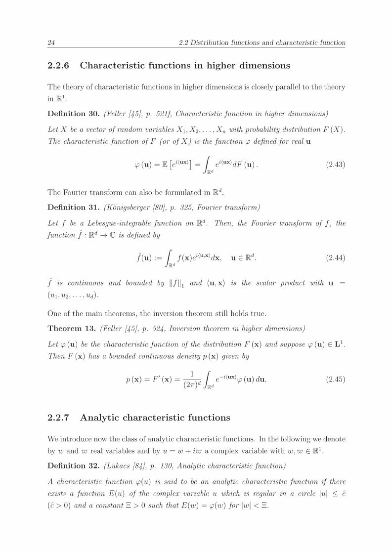
The theory of characteristic functions in higher dimensions is closely parallel to the theory
in R1.
Definition 30. (Feller [45], p. 521f, Characteristic function in higher dimensions)
Let X be a vector of random variables X1, X2, . . . , Xn with probability distribution F (X).
The characteristic function of F (or of X) is the function ϕ defined for real u
ϕ (u) = E[ei〈ux〉
]=
∫
Rd
ei〈ux〉dF (u) . (2.43)
The Fourier transform can also be formulated in Rd.
Definition 31. (Konigsberger [80], p. 325, Fourier transform)
Let f be a Lebesgue-integrable function on Rd. Then, the Fourier transform of f , the
function f : Rd → C is defined by
f(u) :=
∫
Rd
f(x)ei〈u,x〉dx, u ∈ Rd. (2.44)
f is continuous and bounded by ‖f‖1 and 〈u,x〉 is the scalar product with u =
(u1, u2, . . . , ud).
One of the main theorems, the inversion theorem still holds true.
Theorem 13. (Feller [45], p. 524, Inversion theorem in higher dimensions)
Let ϕ (u) be the characteristic function of the distribution F (x) and suppose ϕ (u) ∈ L1.
Then F (x) has a bounded continuous density p (x) given by
p (x) = F ′ (x) =1
(2π)d
∫
Rd
e−i〈ux〉ϕ (u) du. (2.45)
2.2.7 Analytic characteristic functions
We introduce now the class of analytic characteristic functions. In the following we denote
by w and real variables and by u = w + i a complex variable with w, ∈ R1.
Definition 32. (Lukacs [84], p. 130, Analytic characteristic function)
A characteristic function ϕ(u) is said to be an analytic characteristic function if there
exists a function E(u) of the complex variable u which is regular in a circle |u| ≤ c
(c > 0) and a constant Ξ > 0 such that E(w) = ϕ(w) for |w| < Ξ.

2 Mathematical preliminaries and definitions 25
This can be expressed in an informal manner (see [84], p. 130) by saying that an analytic
characteristic function is a characteristic function which coincides with a holomorphic
function in some neighbourhood of the origin in the complex u-plane.
Theorem 14. (Lukacs [84], Theorem 7.1.1, p. 132)
If a characteristic function ϕ(u) is regular in a neighbourhood of the origin, then it is
also regular in a horizontal strip and can be represented in this strip by a Fourier integral.
This strip is either the whole plane, or it has one or two horizontal lines. The purely
imaginary points on the boundary of the strip of regularity (if this strip is not the whole
plane) are singular points of ϕ(u).
A proof can be found in [84], p. 130ff. The following example is based on an example in
[85].
Example 1. Take the characteristic function
ϕ(u) = (1− iu
a)−1, (2.46)
with a ∈ R. This function satisfies the elementary necessary conditions for characteristic
functions, namely ϕ(−u) = ϕ(u), ϕ(0) = 1, |ϕ(u)| ≤ 1 for real u. It has a singularity on
the imaginary axis in u = −ia, i.e. the function is regular near the origin in the strip
−a ≤ ℑ(u) ≤ ∞, where ℑ(u) denotes the imaginary part of u (see Figure 2.1). In this
example we find that the strip of regularity is bounded by one horizontal line in ℑ(u) = a.
Boundary line
Strip of regularity
−1 −0.8 −0.6 −0.4 −0.2 0 0.2 0.4 0.6 0.8 1−2.5
−2
−1.5
−1
−0.5
0
0.5
1
Figure 2.1: Strip of analyticity
Thus, for a < ℑ(u) < b, where ℑ(u) denotes the imaginary part of u, the characteristic

26 2.2 Distribution functions and characteristic function
function of the process X(t) is identical to the generalized Fourier transform of the tran-
sition density. We use here the concept of the complex Fourier transform by Titchmarsh
[113], p. 4ff and 42ff: The existence of the integral defining f implies a certain restriction
on f(x) at infinity. But even if f does not exist, the functions
f+(u) =
∫ ∞
0
f(x)eiuxdx, (2.47)
f−(u) =
∫ 0
−∞f(x)eiuxdx, (2.48)
where u = w + i, may exist, the former for sufficiently large positive , the latter for
sufficiently large negative . For
f+(u) =
∫ ∞
0
f(x)e−xeiwxdx, (2.49)
so that f+ is the transform of the function equal to f(x)e−x for x > 0, and to 0 for
x < 0. For the inversion we may write
f(x) =1
2π
(∫ ia1+∞
ia1−∞f+(u)e
ixudu+
∫ ib1+∞
ib1−∞f−(u)e
−ixudu
)
, (2.50)
where a1 is a sufficiently large positive number, b1 a sufficiently large negative number.
In this context the next three theorems, the Cauchy integral theorem, the Cauchy integral
formula and the Residue theorem, are quite helpful.
Definition 33. ([63], Simply-connected domain)
In a simply-connected domain D any closed path can be continuously deformed into a
point, remaining the whole time in the simply-connected domain D.
Theorem 15. ([63], Cauchy integral theorem)
If f(u) is a holomorphic function of a complex variable u in a simply-connected domain D
in the complex plane C, then the integral of f(u) along any closed rectifiable (i.e. having
finite length) curve γ in D vanishes:
∫
γ
f(u)du = 0. (2.51)
An equivalent version of Cauchy’s integral theorem states that the integral
∫ b
a
f(u)du, a, b ∈ D, (2.52)
2 Mathematical preliminaries and definitions 27
is independent of the choice of the path of integration (contour) between the fixed points
a and b in D.
Theorem 16. (Konigsberger [80], p. 203, [100], Cauchy integral formula)
If f is a holomorphic function in an open domain D which includes the closure of the disk
Kr(a) = u : |u− a| ≤ r then for every point u0 ∈ Kr(a)
f(u0) =1
2πi
∫
γ
f(u)
u− u0du, (2.53)
where γ denotes the circle which forms the boundary of Kr. This formula can be extended
to two dimensions. If f is a function which is holomorphic in its variables u1 and u2 in
an open domain D which includes Kr(a1, a2) = ui : |ui − ai| ≤ ri, i = 1, 2 then for every
point (u10, u20) ∈ Kr(a1, a2)
f(u10, u20) =1
(2πi)2
∫
Γ
f(u1, u2)
(u1 − u10)(u2 − u20)du1du2, (2.54)
where Γ = ui : |ui − ai| = ri, i = 1, 2.
Definition 34. ([63], Residue)
Let f(u) be a function of one complex variable and f has a finite isolated singular point
at a. The integral
Resaf :=1
2πi
∫
γ
f(u)du, (2.55)
where γ is a counter-clockwise oriented circle of sufficiently small radius with centre at a,
is called residue of f in a.
Remark 1. If f has a simple pole at a the residue of f is given by
Resaf = limu→a
((u− a)f(u)) . (2.56)
See [63].
Theorem 17. ([63], Residue theorem)
Let f be a single-valued analytic function everywhere in a simply-connected domain D,
except for isolated singular points; then the integral of f(u) over any counter-clockwise
oriented, simple (i.e. injective) closed rectifiable curve γ lying in D and not passing through
the singular points of f(u) can be computed by the formula
∫
γ
f(u)du = 2πin∑
k=1
Resakf(u), (2.57)

28 2.2 Distribution functions and characteristic function
where ak, k = 1, . . . , n, are the singular points of f(u) inside γ.
Corollary 2. (Contour variation in the strip of regularity)
Assume a function f(u), u = w + i, analytic in a strip a < ℑ(u) < b which decays
at ±∞ like e−c1|u|. Then it follows from Cauchy’s theorem that the integral over f(u)
extending from −∞ to +∞ can be taken along any line in the strip of regularity parallel
to the real axis.
If f(u) = g(u)h(u), where g(u), h(u) are analytic in a strip a < ℑ(u) < b, g(u) bounded
and h(u) decays at ±∞ like e−c1|u| then it also follows from Cauchy’s theorem that an
integral over f(u) = g(u)h(u) extending from −∞ to +∞ can be taken along any line of
the strip of regularity parallel to the real axis.
See also Titchmarsh [113], p. 44f.
Proof.
Assume that we take the integral along a line in the strip of regularity at ℑ(u) = c1 from
−∞ to +∞:
Γ1 =
∫ ∞+ic1
−∞+ic1
f(u)du (2.58)
Assume a second line ℑ(u) = c2 parallel to ℑ(u) = c1, which also must be within the strip
of regularity.
ℑ(u)
−A A ℜ(u)
c1
c2
Γ2 Γ4
Γ3
Γ1Strip of regularity
Figure 2.2: Contour variation within strip of regularity
By Cauchy’s theorem this integral is equal to the sum of three integrals, which build with
−Γ1 a closed curve,
Γ1 =
∫ −∞+ic2
−∞+ic1
f(u)du
︸ ︷︷ ︸
=Γ2
+
∫ ∞+ic2
−∞+ic2
f(u)du
︸ ︷︷ ︸
=Γ3
+
∫ ∞+ic1
∞+ic2
f(u)du
︸ ︷︷ ︸
=Γ4
. (2.59)
2 Mathematical preliminaries and definitions 29
For Γ2 and Γ4 we derive due to the decay e−c1|u| of f(u) at ±∞
limA→−∞
∫ A+ic2
A+ic1
f(u)du ≈ limA→−∞
∫ A+ic2
A+ic1
e−c1|u|︸ ︷︷ ︸
≤e−c1w
du
≤ limA→−∞
e−c1|A|dw
= 0,
limA→∞
∫ A+ic1
A+ic2
f(u)du = 0. (2.60)
Thus, Γ1 = Γ3 and the first part of the corollary follows. If f(u) = g(u)h(u), with g(u)
bounded, then Γ2 and Γ3 are given by
limA→−∞
∫ A+ic2
A+ic1
g(u)h(u)du ≤ limA→−∞
∫ A+ic2
A+ic1
c3e−c1|u|du
= 0,
limA→∞
∫ A+ic1
A+ic2
f(u)du = 0. (2.61)
Corollary 3. (Residue calculus, contour variation in a strip with simple poles)
Assume a function f(u) which decays at ±∞ like e−c1|u|. Furthermore, f(u) regular in a
strip a < ℑ(u) < b and except for simple poles at a and b it is regular in an even larger
strip S∗f . Then it follows from Cauchy’s theorem and the Residue theorem that the integral
over f(u) extending from −∞ to +∞ can be taken along any line c2 in S∗f parallel to the
real axis taking into account the contribution of the residue the contour has been moved
across or along. The residue contribution is given by
−2πiResaf for c2 < a,
−2πiResbf for c2 > b,
−πiResaf for c2 = a,
−πiResbf for c2 = b.
(2.62)
Assume f(u) = g(u)h(u) with g(u) bounded and h(u) decays at ±∞ like e−c1|u|. Moreover,
g(u), h(u) are regular in a strip a < ℑ(u) < b and except for simple poles at a and b they
are regular in an even larger strip S∗f . Then it follows from Cauchy’s theorem and the
Residue theorem that the integral over f(u) = g(u)h(u) extending from −∞ to +∞ can
be taken along any line in S∗f parallel to the real axis taking into account the residue
contribution.

30 2.2 Distribution functions and characteristic function
Proof.
Assume that we take the integral along a line in the strip of regularity at ℑ(u) = c1 from
−∞ to +∞:
Γ1 =
∫ ∞+ic1
−∞+ic1
f(u)du (2.63)
Assume a second line ℑ(u) = c2 parallel to ℑ(u) = c1 with c2<
(=) a.
ℑ(u)
−A A ℜ(u)
c1
c2
Γ2 Γ4
Γ3
Γ1Strip of regularity
γ−
Figure 2.3: Contour variation with simple poles
By Cauchy’s theorem this integral is equal to the sum of four integrals, which build with
−Γ1 a closed curve,
Γ1 =
∫ −∞+ic2
−∞+ic1
f(u)du
︸ ︷︷ ︸
=Γ2
+
∫ ∞+ic2
−∞+ic2
f(u)du
︸ ︷︷ ︸
=Γ3
+
∫ ∞+ic1
∞+ic2
f(u)du
︸ ︷︷ ︸
=Γ4
+
(1
2
)
︸ ︷︷ ︸
for c2=a
∫
γ−
f(u), (2.64)
where γ− describes a circle, in clockwise direction, of sufficiently small radius with cen-
tre at a. According to the Residue theorem this integral is then given by −2πiResaf(−πiResaf respectively). The results for c2 > b follow accordingly. From the above proof
we also know that Γ2 = 0 and Γ4 = 0.
The second part of the corollary follows analogously with Corollary 2.
2 Mathematical preliminaries and definitions 31
2.3 The Ito formula and the martingale representa-
tion theorem
In our context we work with so called Ito processes.
Definition 35. (Zagst [119], Definition 2.32, p. 27f, Ito process)
Let W (t) be a d-dimensional Wiener process, d ∈ N. A stochastic process X = (X(t))t≥0
is called an Ito process if for all t ≥ 0 we have
X(t) = X(0) +
∫ t
0
µ (s,X(s)) ds+
∫ t
0
σ (s,X(s)) dW (s)
= X(0) +
∫ t
0
µ (s,X(s)) ds+d∑
k=1
∫ t
0
σk (s,X(s)) dWk(s), (2.65)
where X(0) is (F0−) measurable and µ = (µ(t))t≥0 and σ = (σ(t))t≥0 with σ(t) =
(σ1(t), . . . , σd(t))t≥0 are a one and a d-dimensional progressively measurable stochastic
process with
∫ t
0
|µ (s,X(s))| ds <∞, (2.66)
∫ t
0
σ2k (s,X(s)) ds <∞, Q− a.s. for all t ≥ 0, k = 1, . . . , d. (2.67)
A d-dimensional Ito process is given by a vector X = (X1, . . . , Xd), d ∈ N, with each Xi
being an Ito process, i = 1, . . . , d.
Remark 2. For convenience we write (2.65) symbolically
dX(t) = µ (t,X(t)) dt+ σ (t,X(t)) dW (t)
= µ (t,X(t)) dt+d∑
k=1
σk (t,X(t)) dWk(t), (2.68)
and call this stochastic differential equation (SDE) with drift parameter µ and diffusion
parameter σ.
To use Ito’s Lemma we have to define the quadratic covariance process.
32 2.3 The Ito formula and the martingale representation theorem
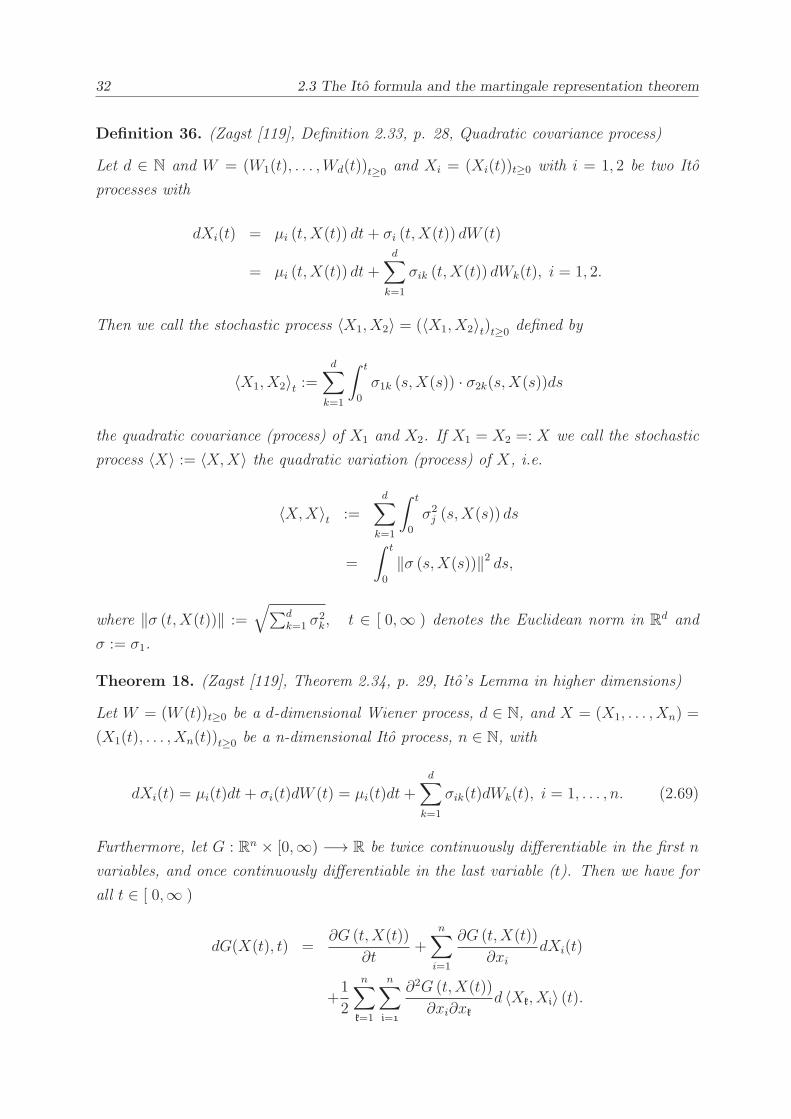
Definition 36. (Zagst [119], Definition 2.33, p. 28, Quadratic covariance process)
Let d ∈ N and W = (W1(t), . . . ,Wd(t))t≥0 and Xi = (Xi(t))t≥0 with i = 1, 2 be two Ito
processes with
dXi(t) = µi (t,X(t)) dt+ σi (t,X(t)) dW (t)
= µi (t,X(t)) dt+d∑
k=1
σik (t,X(t)) dWk(t), i = 1, 2.
Then we call the stochastic process 〈X1, X2〉 = (〈X1, X2〉t)t≥0defined by
〈X1, X2〉t :=d∑
k=1
∫ t
0
σ1k (s,X(s)) · σ2k(s,X(s))ds
the quadratic covariance (process) of X1 and X2. If X1 = X2 =: X we call the stochastic
process 〈X〉 := 〈X,X〉 the quadratic variation (process) of X, i.e.
〈X,X〉t :=d∑
k=1
∫ t
0
σ2j (s,X(s)) ds
=
∫ t
0
‖σ (s,X(s))‖2 ds,
where ‖σ (t,X(t))‖ :=√∑d
k=1 σ2k, t ∈ [ 0,∞ ) denotes the Euclidean norm in R
d and
σ := σ1.
Theorem 18. (Zagst [119], Theorem 2.34, p. 29, Ito’s Lemma in higher dimensions)
Let W = (W (t))t≥0 be a d-dimensional Wiener process, d ∈ N, and X = (X1, . . . , Xn) =
(X1(t), . . . , Xn(t))t≥0 be a n-dimensional Ito process, n ∈ N, with
dXi(t) = µi(t)dt+ σi(t)dW (t) = µi(t)dt+d∑
k=1
σik(t)dWk(t), i = 1, . . . , n. (2.69)
Furthermore, let G : Rn × [0,∞) −→ R be twice continuously differentiable in the first n
variables, and once continuously differentiable in the last variable (t). Then we have for
all t ∈ [ 0,∞ )
dG(X(t), t) =∂G (t,X(t))
∂t+
n∑
i=1
∂G (t,X(t))
∂xidXi(t)
+1
2
n∑
k=1
n∑
i=1
∂2G (t,X(t))
∂xi∂xkd 〈Xk, Xi〉 (t).

2 Mathematical preliminaries and definitions 33
The following theorem shows that each continuous local martingale relative to (Q,F(W )),
i.e. relative to Q and the natural filtration F(W ), can be written as an Ito process. In
the following we denote these martingales briefly (Q−) martingales.
Theorem 19. (Zagst [119], Theorem 2.38, p. 31, Martingale representation I)
Let d ∈ N, W = (W1(t), . . . ,Wd(t))t≥0 be a d-dimensional Wiener process, and M =
(M(t))t∈[0,T ] be a continuous local (Q−) martingale. Then there is a progressively mea-
surable process φ = (φ(t))t∈[0,T ] , φ : [0, T ]× Ω −→ Rd such that
i.∫ T
0‖φ(t)‖2 dt <∞ Q− a.s.,
ii. M(t) = M(0) +∫ t
0φ(s)′dW (s) or briefly dM(t) = φ(t)′dW (t) Q− a.s. for all
t ∈ [0, T ], where φ(s)′ is the transposed of φ(s).
If M = (M(t))t∈[0,T ] is a continuous (Q−) martingale with EQ [M2(t)] < ∞ for all t ∈[0, T ], then 1. is strengthened to
EQ
[∫ T
0
‖φ(t)‖2 dt]
<∞,
while 2. still holds.
For a proof see Øksendal [91], p. 53-54.
Lemma 1. (Zagst [119], Lemma 2.40, p. 33, Novikov condition)
Let γ = (γ(t))t>0 be a d-dimensional progressively measurable stochastic process, d ∈ N,
with ∫ t
0
γ2k(s)ds <∞, Q− a.s. for all t ≥ 0, k = 1, . . . , d
and let the stochastic process E (γ) = (E (t, γ))t≥0 = (E (t, γ(t)))t≥0 for all t ≥ 0 be defined
by
E (t, γ) = e−∫ t0 γ(s)′dW (s)− 1
2
∫ t0 ‖γ(s)‖
2ds.
Then E (γ) is a continuous (Q−) martingale if
EQ
[
e12
∫ T0 ‖γ(s)‖2ds
]
<∞. (Novikov condition)
For a proof see Karatzas and Shreve [76], p. 198-199.
Remark 3. Under Novikov’s condition it is true that
∫ T
0
‖γ(s)‖2 ds <∞, Q− a.s.

34 2.4 Diffusions and stochastic differential equations
and ∫ t
0
‖γ(s)‖2 ds <∞, Q− a.s. for all t ∈ [0, T ].
Remark 4. For each T ≥ 0 we define the measure Q = QE(T,γ) on the measure space
(Ω,FT ) by
Q (A) := EQ [1A · E (T, γ)] =∫
A
E (T, γ) dQ for all A ∈ FT ,
which is a probability measure if E (T, γ) is a Q-martingale. In this case, E (T, γ) is the
Q-density of Q, i.e. E (T, γ) = dQdQ on (Ω,FT ).
We provide the Girsanov theorem, which shows, how a(
Q−)
Wiener process W =(
W (t))
t∈[0,T ]starting with a (Q−) Wiener process W = (W (t))t≥0 can be constructed.
Theorem 20. (Zagst [119], Theorem 2.41, p. 34f, Girsanov theorem)
Let W = (W1(t), . . . ,Wd(t))t≥0 be a d-dimensional (Q−) Wiener process, d ∈N, γ, E (γ) , Q, and T ∈ [ 0,∞ ) be as defined above, and the d-dimensional stochastic
process W =(
W1, . . . , Wd
)
=(
W1(t), . . . , Wd(t))
t∈[0,T ]be defined by
Wk(t) := Wk(t) +
∫ t
0
γk(s)ds, t ∈ [0, T ], k = 1, . . . , d,
i.e.
dW (t) := γ(t)dt+ dW (t), t ∈ [0, T ].
If the stochastic process E (γ) = (E (t, γ))t∈[0,T ] is a (Q−) martingale, then the stochastic
process W is a d-dimensional(
Q−)
Wiener process on the measure space (Ω,FT ).
For γ(t) constant the change of measure corresponds to a change of the drift from µ to
µ− γ. For a proof see Øksendal [91], p. 163-164.
2.4 Diffusions and stochastic differential equations
In this section we want to analyse the question of existence and uniqueness for solutions
to stochastic differential equations. According to Karatzas and Shreve [76], p. 281ff,
this endeavour is really a study of diffusion processes. Loosely speaking, a diffusion is a
Markov process which has continuous sample paths and can be characterised in terms of
its infinitesimal generator.
2 Mathematical preliminaries and definitions 35
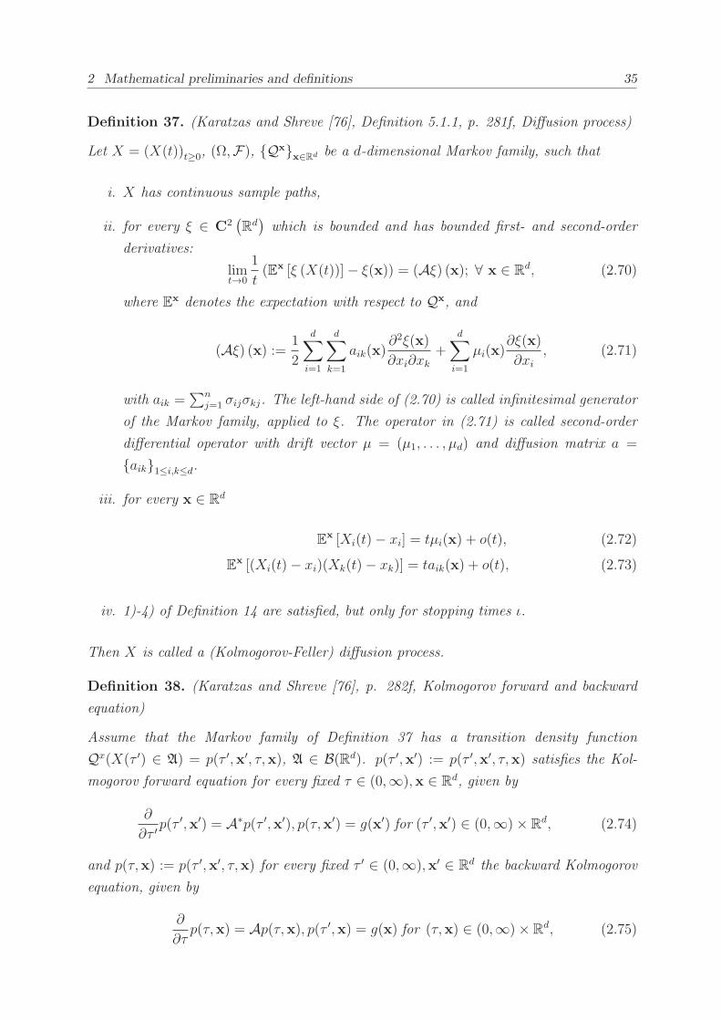
Definition 37. (Karatzas and Shreve [76], Definition 5.1.1, p. 281f, Diffusion process)
Let X = (X(t))t≥0, (Ω,F), Qxx∈Rd be a d-dimensional Markov family, such that
i. X has continuous sample paths,
ii. for every ξ ∈ C2(R
d)which is bounded and has bounded first- and second-order
derivatives:
limt→0
1
t(Ex [ξ (X(t))]− ξ(x)) = (Aξ) (x); ∀ x ∈ R
d, (2.70)
where Ex denotes the expectation with respect to Qx, and
(Aξ) (x) := 1
2
d∑
i=1
d∑
k=1
aik(x)∂2ξ(x)
∂xi∂xk+
d∑
i=1
µi(x)∂ξ(x)
∂xi, (2.71)
with aik =∑n
j=1 σijσkj. The left-hand side of (2.70) is called infinitesimal generator
of the Markov family, applied to ξ. The operator in (2.71) is called second-order
differential operator with drift vector µ = (µ1, . . . , µd) and diffusion matrix a =
aik1≤i,k≤d.
iii. for every x ∈ Rd
Ex [Xi(t)− xi] = tµi(x) + o(t), (2.72)
Ex [(Xi(t)− xi)(Xk(t)− xk)] = taik(x) + o(t), (2.73)
iv. 1)-4) of Definition 14 are satisfied, but only for stopping times ι.
Then X is called a (Kolmogorov-Feller) diffusion process.
Definition 38. (Karatzas and Shreve [76], p. 282f, Kolmogorov forward and backward
equation)
Assume that the Markov family of Definition 37 has a transition density function
Qx(X(τ ′) ∈ A) = p(τ ′,x′, τ,x), A ∈ B(Rd). p(τ ′,x′) := p(τ ′,x′, τ,x) satisfies the Kol-
mogorov forward equation for every fixed τ ∈ (0,∞),x ∈ Rd, given by
∂
∂τ ′p(τ ′,x′) = A∗p(τ ′,x′), p(τ,x′) = g(x′) for (τ ′,x′) ∈ (0,∞)× R
d, (2.74)
and p(τ,x) := p(τ ′,x′, τ,x) for every fixed τ ′ ∈ (0,∞),x′ ∈ Rd the backward Kolmogorov
equation, given by
∂
∂τp(τ,x) = Ap(τ,x), p(τ ′,x) = g(x) for (τ,x) ∈ (0,∞)× R
d, (2.75)
36 2.4 Diffusions and stochastic differential equations
where the adjoint operator A∗ is given by
(A∗p) (τ ′,x′) :=1
2
d∑
i=1
d∑
k=1
∂2
∂x′i∂x′k
(aik (τ′,x′) p (τ ′,x′))−
d∑
i=1
∂
∂x′i(µi (τ
′,x′) p (τ ′,x′)) ,
(2.76)
if the derivatives are bounded and Holder-continuous. (τ ′,x′) describe the forward vari-
ables, while (τ,x) are the backward variables, i.e. τ ′ ≥ τ .
Remark 5. The following equation with terminal condition
− ∂
∂tp(t,x) = Ap(t,x); t′,x′ fixed, for (t,x) ∈ (0,∞)× R
d; p(t′,x) = g(x), (2.77)
can be easily transformed into the backward Kolmogorov equation presented before with
initial condition by the transformation τ = t′ − t (time reversal):
∂
∂τp(τ,x) = Ap(τ,x); τ ′,x′ fixed, for (τ,x) ∈ (0,∞)× R
d; p(0,x) = g(x). (2.78)
For the specific Kolmogorov equations of the models we treat in the main part refer to
Appendix A.1.1.
Theorem 21. (Øksendal [91], Theorem 8.1.1, p. 139f, Kolmogorov’s backward equation)
Let g ∈ C20(R
d). Define1
ξ(τ,x) = Eτ,x [g (X(0))] . (2.79)
Then
∂ξ
∂τ= Aξ, τ > 0,x ∈ R
d, (2.80)
ξ(0,x) = g(x), x ∈ Rd. (2.81)
Moreover, if h(τ,x) ∈ C1,2(R× R
d)is a bounded function satisfying (2.80) and (2.81),
then h(τ,x) = ξ(τ,x), given by (2.79).
Definition 39. (Fouque et al. [49], p. 62f, Invariant probability density)
The existence of an invariant probability density means that p(t′, x′, t, x) does not depend
on t′ or t and consequently satisfies
A∗p = 0. (2.82)
1Note that we have reversed the time by setting τ = T − t, i.e. τ = 0 means t = T .

2 Mathematical preliminaries and definitions 37
Definition 40. ([63], Symmetric difference)
The symmetric difference of the sets A and B is denoted by
A B. (2.83)
The symmetric difference is equivalent to the union of both relative complements, i.e.
A B = (A \B) ∪ (B \ A). (2.84)
Definition 41. ([63], Measure-preserving transformation)
A measurable mapping T : Ω1 → Ω2, i.e. a mapping T from measure space (Ω1,F1,Q1)
to (Ω2,F2,Q2) with T−1(A2) = x : T(x) ∈ A2 ∈ F1 for each A2 ∈ F2, such that
Q1(T−1(A2)) = Q2(A2) for every A2 ∈ F2 is called a measure-preserving transforma-
tion.
Theorem 22. (Walters [117], Theorem 1.5, p. 27, Ergodicity)
If T : Ω → Ω is a measure-preserving transformation of the probability space (Ω,F ,Q),then the following statements are equivalent:
i. T is ergodic.
ii. The only members A1 of F with Q (T−1(A1) A1) = 0 are those with Q (A1) = 0
or Q (A1) = 1.
iii. For every A1 ∈ F with Q (A1) > 0 we have Q (⋃∞
n=1 T−n(A1)) = 1, where Tn denotes
the nth iterate of the transformation T and T−n its inverse.
iv. For every A1,A2 ∈ F with Q (A1), Q (A2) > 0 there exists n > 0 with
Q (T−n(A1)⋂
A2) > 0.
For a proof see [117], p. 27f.
Theorem 23. (Fouque [54], p. 115, Ergodicity of Markov processes)
Let us assume a Markov process, which is irreducible, i.e. the process can visit any neigh-
bourhood of the state space with positive probability, in finite time and from any starting
point, and which possesses an invariant probability density function. Then the process is
ergodic.
38 2.4 Diffusions and stochastic differential equations
Remark 6. Every ergodic Markov process has a unique invariant probability distribution
pinv and the distribution converges to the invariant distribution as t→∞ for any initial
distribution. This probability distribution belongs to the null space of the adjoint generator
A∗ of its infinitesimal generator A, i.e. that is the invariant distribution solves the adjoint
equation: A∗ pinv=0.
See [54], p. 116.
Instead of proving the existence of a Markov process X satisfying the Kolmogorov back-
ward and forward equation, the methodology of stochastic differential equations was sug-
gested. Thus, in the following we introduce the concept of stochastic differential equations
with respect to Brownian motions and their solutions in the so-called strong sense.
Definition 42. (Zagst [119], Definition 2.44, p. 36, Strong solution)
If there exists a d-dimensional stochastic process X = (X(t))t≥0 on the filtered probability
space (Ω,F ,Q,F), where each satisfies (2.66) and (2.67), i.e. an Ito process, such that
for all t ≥ 0
X(t) = x+
∫ t
0
µ(s,X(s))ds+
∫ t
0
σ(s,X(s))dW (s) Q− a.s.,
X(0) = x ∈ Rd, fixed, (2.85)
we call X a strong solution of the stochastic differential equation
dX(t) = µ(t,X(t))dt+ σ(t,X(t))dW (t), for all t ≥ 0,
X(0) = x. (2.86)
The following theorem answers the existence and uniqueness question for some stochastic
differential equations.
Theorem 24. (Zagst [119], Theorem 2.45, p. 36f, Existence and Uniqueness)
Let µ and σ of the stochastic differential equation be continuous functions such that for
all t ≥ 0,x,y ∈ Rn and for some constant Ξ1 > 0 the following conditions hold:
i. (Lipschitz condition)
‖µ(t,x)− µ(t,y)‖+ ‖σ(t,x)− σ(t,y)‖ ≤ Ξ1 ‖x− y‖ , (2.87)
ii. (Growth condition)
‖µ(t,x)‖2 + ‖σ(t,x)‖2 ≤ Ξ21(1 + ‖x‖2). (2.88)

2 Mathematical preliminaries and definitions 39
Then there exists a unique, continuous strong solution X = (X(t))t≤0 of the SDE and a
constant Ξ2, depending only on Ξ1 and T > 0, such that
EQ[‖X(t)‖2
]≤ Ξ2(1 + ‖x‖2)eΞ2t for all t ∈ [0, T ]. (2.89)
Moreover,
EQ
[
sup0≤t≤T
‖X(t)‖2]
<∞.
For a proof see Øksendal [91], p. 69-71.
In the one dimensional case, the Lipschitz condition on the diffusion coefficient can be
considerably relaxed.
Proposition 1. (Karatzas and Shreve [76], Proposition 5.2.13, p. 291, Yamada and
Watanabe)
Let d = 1 and let us suppose that the coefficients of the one-dimensional equation
dX(t) = µ(t,X(t))dt+ σ(t,X(t))dW (t) (2.90)
satisfy the conditions
|µ(t, x)− µ(t, y)| ≤ Ξ1 |x− y| ,|σ(t, x)− σ(t, y)| ≤ h |x− y| ,
for every 0 ≤ t <∞ and x ∈ R, y ∈ R, where Ξ1 is a positive constant and h : [0,∞) 7−→[0,∞) is a strictly increasing function with h(0) = 0 and
∫
0,Ξ2
h−2(u)du =∞; ∀ Ξ2 > 0. (2.91)
Then strong uniqueness holds for Equation (2.90).
For a proof see Karatzas and Shreve[76], p. 291-292.
Definition 43. (Karatzas and Shreve [76], Definition 5.3.1, p. 300, Weak solution)
A weak solution of Equation (2.65) is a tuple (X,W ), (Ω,F ,Q,F), where
i. (Ω,F ,Q) is a probability space, and F is a filtration of sub-σ-fields of F satisfying
the usual conditions,
ii. X = X(t),Ft, 0 ≤ t <∞ is a continuous, adapted Rd-valued process,
W = W (t),Ft, 0 ≤ t <∞ is a d-dimensional Brownian motion,
40 2.4 Diffusions and stochastic differential equations
iii. Q(∫ t
0(|µ (s,X(s))|+ σ2
k (s,X(s)) ds) <∞)
= 1 holds for every 1 ≤ k ≤ d, and
0 ≤ t <∞, and
iv. the integral version of (2.65)
X(t) = X(0) +
∫ t
0
µ (s,X(s)) ds+
∫ t
0
σ (s,X(s)) dW (s), 0 ≤ t <∞. (2.92)
holds almost surely.
2.4.1 Important examples of SDE’s in R1
Example 2. (Geometric Brownian Motion)
We model the stock prices with geometric Brownian motions with the following SDE
dX(t) = X(t) (µdt+ σdW (t)) , X(0) > 0, (2.93)
where µ and σ are fixed constants.
This differential equation has the unique solution
X(t) = X(0)e(µ−12σ2)t+σW (t). (2.94)
For a proof see Bingham and Kiesel [12], p. 215-216.
Furthermore, the expectation, variance, and covariance functions are (see Arcones [6], p.
178)
E [X(t)] = X(0)eµt, (2.95)
Var [X(t)] = X(0)2e2µt(eσ2t − 1), (2.96)
Cov [X(s), X(t)] = X(0)2eµ(t+s)(eσ2(t∧s) − 1). (2.97)
Example 3. (Ornstein-Uhlenbeck Process)
The oldest example of a stochastic differential equation is the Ornstein-Uhlenbeck (OU)
Process (see Bingham and Kiesel [12], p. 204)
dX(t) = −κX(t)dt+ σdW (t), X(0) > 0, (2.98)
2 Mathematical preliminaries and definitions 41
The solution of this equation is (see Karatzas and Shreve [76], p. 358)
X(t) = X(0)e−κt + σ
∫ t
0
e−κ(t−s)dW (s); 0 ≤ t <∞. (2.99)
The expectation, variance, and covariance functions are (see Karatzas and Shreve [76], p.
358)
E [X(t)] = X(0)e−κt, (2.100)
Var [X(t)] =σ2
2κ(1− e−2κt), (2.101)
Cov [X(s), X(t)] =σ2
2κe−κ(t+s)(e2κ(t∧s) − 1). (2.102)
The invariant distribution of X is a zero-mean Gaussian distribution with covariance
function Cov(X(s), X(t)) = (σ2/2κ) e−κ|t−s|.
A special case is the mean-reverting Ornstein-Uhlenbeck process (see Øksendal [91], p. 75)
dX(t) = κ (ζ −X (t)) dt+ σdW (t), (2.103)
which can be solved for
X(t) = ζ(1− e−κt
)+X(0)e−κt + σ
∫ t
0
e−κ(t−s)dW (s); 0 ≤ t <∞. (2.104)
See Øksendal [91], p. 75. The expectation, variance, and covariance functions are given
by
E [X(t)] = ζ(1− e−κt
)+X(0)e−κt, (2.105)
Var [X(t)] =σ2
2κ(1− e−2κt), (2.106)
Cov [X(s), X(t)] =σ2
2κe−κ(t+s)(e2κ(t∧s) − 1). (2.107)
X(t) is mean-reverting, i.e.
E [X(t)] = ζ(1− e−κt
)+X(0)e−κt −→ ζ, (2.108)
as t −→ ∞. The invariant distribution is, thus, a Gaussian with mean ζ and covariance
function Cov(X(s), X(t)) = (σ2/2κ) e−κ|t−s|.
42 2.4 Diffusions and stochastic differential equations
Example 4. (Cox-Ingersoll-Ross Process (CIR))
dX(t) = κ (ζ −X(t)) dt+ σ√
X(t)dW (t). (2.109)
Cox, Ingersoll, Ross applied this process to model interest rates, Heston used it to describe
the volatility in his model, because X(t) remains positive (if X(0) ≥ 0) provided (see Feller
[43])
ζ >σ2
2κ. (2.110)
Its existence and uniqueness can be proved with the Yamada-Watanabe proposition (Propo-
sition 1). For this process there is no explicit formula for X(t) in terms ofW (t). However,
there exists an explicit formula for the transition probability density
p ((t, x) −→ (s, y)) = p (X(s) = y | X(t) = x) . (2.111)
See Cox, Ingersoll and Ross [25].
The expectation and the variance are given by (see [30])
E [X(t)] = X(0)e−κt + ζ(1− e−κt
), (2.112)
Var [X(t)] = X(0)σ2
κ
(e−κt − e−2κt
)+ ζ
σ2
2κ
(1− e−2κt
)2. (2.113)
Cov [X(s), X(t)] = X(0)σ2
κ(e−κt − e−κ(s+t))
+ζσ2
2κ(e−κ(t−s) − 2e−κt + e−κ(t+s)), s < t (2.114)
As the CIR process is mean-reverting:
E [X(t)] = X(0)e−κt + ζ(1− e−κt
)−→ ζ. (2.115)
The invariant distribution of the CIR process is the gamma distribution with expectation
ζ and variance ζ σ2
2κ[36].
2 Mathematical preliminaries and definitions 43
2.5 Connections between stochastic differential equa-
tions and partial differential equations
A direct link is given by the Feynman-Kac representation. In the following we consider a
solution to the stochastic differential Equation (2.65), under the assumptions that
i. the coefficients µi(t,x) and σik(t,x) are continuous and satisfy the linear growth
condition (2.88),
ii. the Equation (2.65) has a weak solution(X(t,x),W
), (Ω,F ,Q,F) for every pair
(t,x) with X(t) = x, and that
iii. the solution is unique in the sense of probability law.
Closely related to the Stochastic Differential Equation (2.65) is the second-order differen-
tial operator
(Atξ) (x) :=1
2
d∑
i=1
d∑
k=1
aik(t,x)∂2ξ(x)
∂xi∂xk+
d∑
i=1
µi(t,x)∂ξ(x)
∂xi, ξ ∈ C2
(R
d). (2.116)
With an arbitrary but fixed T > 0 and appropriate constants Ξ > 0, λ ≥ 1, we consider
functions g(x) : Rd → R and r(t, x) : [0, T ]×Rd → [0,∞ ) which are continuous and g(x)
satisfies
|g(x)| ≤ Ξ(
1 + ‖x‖2λ)
or g(x) ≥ 0, ∀ x ∈ Rd. (2.117)
Theorem 25. (Karatzas and Shreve [76], Theorem 5.7.6, p. 366, Feynman-Kac theorem)
Under the preceding assumptions suppose that ξ(t,x) : [ 0, T ]×Rd → R is continuous, is
of class C1,2([ 0, T ]× R
d), and satisfies the Cauchy problem
− ∂ξ
∂t= Atξ − rξ, t > 0, x ∈ R
d, (2.118)
ξ(T,x) = g(x), x ∈ Rd, (2.119)
where we simplified the terminal condition by foregoing the limes-formulation, r is called
killing rate of ξ, as well as the polynomial growth condition
max0≤t≤T
|ξ(t,x)| ≤ Ξ(
1 + ‖x‖2λ)
, x ∈ Rd, (2.120)
for some Ξ > 0, λ ≥ 1. Then ξ(t,x) admits on [0, T ]× Rd the stochastic representation
ξ(t,x) = E(t,x)
[
g (X(T )) exp
−∫ T
t
r(s,X)ds
]
, (2.121)

44 2.5 Connections between stochastic differential equations and partial differential equations
where E(t,x) denotes the expected value with respect to Qt,x with Qt,x(X(t) = x) = 1, on
[0, T ]× Rd. In particular, such a solution is unique.
Definition 44. (Karatzas and Shreve [76], Definition 5.7.9, p. 368, Fundamental solu-
tion)
A fundamental solution of the second-order partial differential Equation (2.118) is a non-
negative function G (t′,x′, t,x) defined for 0 ≤ t < t′ ≤ T , x ∈ Rd, x′ ∈ R
d, with the
property that for every g ∈ C0(Rd), t′ ∈ (0, T ], the function
ξ(t,x) :=
∫
Rd
G (t′,x′, t,x) g (x′) dx′, 0 ≤ t < t′, x ∈ Rd (2.122)
is bounded, of class C1,2, satisfies (2.118) and (2.119).
Theorem 26. (Karatzas and Shreve [76], p. 368 Existence of a fundamental solution)
A fundamental solution G exists if the following conditions imposed on µi(t,x), aik(t,x),
and r(t,x) are satisfied,
i. Uniform ellipticity: There exists a positive constant Ξ such that
d∑
i=1
d∑
k=1
aik(t,x)x′ix
′k ≥ Ξ ‖x′‖2 , (2.123)
holds for every x′ ∈ Rd and (t,x) ∈ [ 0,∞)× R
d,
ii. Boundedness: The functions µi(t,x), aik(t,x), and r(t,x) are bounded in [ 0, T ) ×R
d,
iii. Holder continuity: The functions µi(t,x), aik(t,x), and r(t, x) are (uniformly)
Holder-continuous in [ 0, T )× Rd.
Remark 7. For fixed (t′,x′) ∈ ( 0, T ]× Rd the function
φ(t,x) := G (t′,x′, t,x) (2.124)
is of class C1,2([ 0, T )× R
d)and satisfies the backward Kolmogorov equation in the
backward variables (t,x) with killing rate r and terminal conditions (exactly as in
(2.118)). See Karatzas and Shreve [76], p. 368f.
2 Mathematical preliminaries and definitions 45
If in addition the functions ∂∂xiµi(t,x),
∂∂xiaik(t,x) and ∂2
∂xi∂xkaik(t,x) are bounded and
Holder-continuous, then for fixed (t,x) ∈ ( 0, T ]× Rd the function
ψ (t′,x′) := G(t′,x′, t,x) (2.125)
is of class C1,2([ 0, T )× R
d)and satisfies the forward Kolmogorov equation in the forward
variables (t′,x′) with killing rate r:
∂ψ
∂t′= A∗
t′ψ − rψ, t > 0, x ∈ Rd. (2.126)
See Karatzas and Shreve [76], p. 368f.
With Theorem 25 the solution for ξ is given by
ξ(t,x) = E(x,t)
[
e−∫ t′
tr(s,x)dsg (X(t′))
]
, g ∈ C0
(R
d), t′ ∈ [t, T ]. (2.127)
Comparing (2.127) and (2.122) we can deduce that any fundamental solution G (t′,x′, t,x)
is also the transition probability density for the discounted process X(t,x) determined by
Q(t,x) (X(t′) ∈ A) =
∫
A
G (t′,x′, t,x) dx′, A ∈ B(R
d), 0 ≤ t < t′ ≤ T. (2.128)
In the following our descriptions are based on Zauderer [121], p. 415ff. The here so called
fundamental solution or transition probability is closely related to the Green functions.
This relationship is presented in the following.
Assume that µi(t,x) =12
∑d
k=1∂aik(x)∂xk
then (2.116) can be simplified. In those cases we
call the second-order operator Aselft and reformulate (2.116) to
Aselft ξ(x) =
1
2
d∑
i=1
d∑
k=1
aik(x)∂2ξ(x)
∂xi∂xk+
d∑
i=1
(
1
2
d∑
k=1
∂aik(x)
∂xk
)
∂ξ(x)
∂xi
=1
2
d∑
i=1
d∑
k=1
(
aik(x)∂2ξ(x)
∂xi∂xk+∂aik(x)
∂xk
∂ξ(x)
∂xi
)
=d∑
i=1
d∑
k=1
∂
∂xk
(
aik(x)∂ξ
∂xi
)
. (2.129)
Definition 45. (Reed and Barry [102], p. 186, Adjoint operator)
The adjoint operator A∗ satisfies
〈Aξ, φ〉 = 〈ξ,A∗φ〉. (2.130)

46 2.5 Connections between stochastic differential equations and partial differential equations
An operator for which A = A∗ is called self-adjoint.
We have already given the explicit form of the adjoint operator for a second-order differ-
ential operator in (2.76). Hence,
Aselft
∗ξ(x) =
1
2
d∑
i=1
d∑
k=1
∂2
∂xk∂xi(aik(x)ξ(x))−
d∑
i=1
∂
∂xi
(
1
2
d∑
k=1
∂aik(x)
∂xkξ(x)
)
=1
2
d∑
i=1
d∑
k=1
(
aik(x)∂2ξ(x)
∂xi∂xk+∂aik(x)
∂xk
∂ξ(x)
∂xi
)
+1
2
d∑
i=1
d∑
k=1
(
ξ(x)∂2aik(x)
∂xi∂xk+∂aik(x)
∂xi
∂ξ(x)
∂xk
)
−1
2
d∑
i=1
d∑
k=1
(
ξ(x)∂2aik(x)
∂xi∂xk+∂aik(x)
∂xi
∂ξ(x)
∂xk
)
= Aselft ξ(x) (2.131)
Hence, operators A of the form A =∑d
i=1
∑d
k=1∂
∂xk
(
aik(x)∂ξ
∂xi
)
are self-adjoint. In the
following we work with self-adjoint operators.
Theorem 27. (Zauderer [121], p. 415f, Green function for parabolic equation with
Dirichlet boundary conditions)
For a parabolic equation
∂ξ (t′,x′)
∂t′−Aselfξ (t′,x′) + r(x′)ξ(t′,x′) = K (t′,x′) , x′ ∈ D, 0 < t′, (2.132)
with initial and Dirichlet boundary conditions
ξ (0,x′) = g (x′) , x′ ∈ D, ξ(t′,x′) |x′∈∂D = B (t′,x′) , 0 < t′, (2.133)
where r(x′) is a non-negative function, K(t′,x′) is a real-valued time-dependent function,
D is a bounded region in two or three dimensions and ∂D its boundary. B (t′,x′) is a
given function evaluated on ∂D. The integral theorem for the solution of ξ is then in
(t′,x′)-space:
ξ (t′,x′) =
∫ T
0
∫
D
G (t,x, t′,x′)K (t,x) dxdt+
∫
D
(G (t,x, t′,x′) g(x)
)|t=0 dx
−∫ T
0
∫
∂D
a(t,x)B(t,x)∂G (t,x, t′,x′)
∂ndsdt. (2.134)
where a = aik, ds is an element of the respective boundary area and n denotes the unit
normal on ∂D pointing to the exterior of D. The Green function G(t,x, t′,x′) fulfils the

2 Mathematical preliminaries and definitions 47
following problem
− ∂G (t,x, t′,x′)
∂t−AselfG (t,x, t′,x′) + r(x)G (t,x, t′,x′) = δ (x′ − x) δ (t′ − t) ,
x, x′ ∈ D, 0 < t, t′ < T, (2.135)
with the end and boundary conditions
G (T,x, t′,x′) = 0, G (t,x, t′,x′) |x∈∂D = 0, t ≤ T. (2.136)
The equation (2.135) satisfied by the Green’s function G (t,x, t′,x′) is a backward
parabolic equation that results on reversing the direction of time in the forward parabolic
Equation (2.132). It can be shown that G (t,x, t′,x′) = G (−t′,x′,−t,x, ). Thus, as a
function of x′ and t′, G satisfies a backward parabolic differential equation, but with time
now running forwards instead of backwards. [121], p. 416.
Remark 8. When the time is reversed in the forward parabolic Equation (2.132) by a
change in variables, i.e. t′ → t and we set now K = 0, remove the boundary conditions in
(2.139), then the equation can be reformulated to
− ∂ξ (t,x)
∂t−Aselfξ (t,x) + r(x)ξ(t,x) = 0, x ∈ D, 0 < t < T, (2.137)
with the end conditions
ξ (T,x) = g (x) , x ∈ D, (2.138)
ξ is then given by
ξ (t,x) =
∫
D
(G (t′,x′, t,x) g(x′)
)|t=T dx
′, (2.139)
When we assume that the operator in (2.118) is self-adjoint the two problems are identical.
Thus, (2.139) and (2.122) must agree with each other, which means that the fundamental
solution is equal to the Green function in the backward variables.
The problem of the Green Function (2.135) can be reformulated to be consistent with
the problem the fundamental solution satisfies in the backward variables which we show
in the following. The connecting link between the two formulations lies in Duhamel’s
principle which is now introduced.
48 2.5 Connections between stochastic differential equations and partial differential equations
Theorem 28. (Zauderer [121], p. 218ff, Duhamel’s principle)
Let ξ (t′,x′) satisfy a PDE of parabolic case
∂ξ (t′,x′)
∂t′−Aselfξ (t′,x′) + r(x′)ξ(t′,x′) = K (t′,x′) , (2.140)
with the following initial conditions
ξ (0,x) = 0, (2.141)
and homogeneous boundary conditions (if available). Then there exists a function ϑ(x, t; s)
with parameter s (initial time) such that
ξ (t′,x′) =
∫ t
0
ϑ (t′,x′; s) ds, (2.142)
and ϑ satisfies the following equations
∂ϑ(t′,x′)∂t′
−Aselfϑ (t′,x′) + r(x′)ϑ (t′,x′) = 0, (2.143)
with the same boundary condition (if any) as ξ and the following initial conditions, given
at t = s, where s ≥ 0:
ϑ (s,x) = K (s,x). (2.144)
Remark 9. It can be shown that in the parabolic case the Green function can be alterna-
tively constructed as follows (see [121], p. 417f)
− ∂G (t,x, t′,x′)
∂t−AselfG (t,x, t′,x′) + r(x)G (t,x, t′,x′) = 0, x,x′ ∈ D, t < t′, (2.145)
with the boundary conditions as of before and the initial condition substituted by
G (t′,x, t′,x′) = δ (x′ − x), x′ ∈ D. (2.146)
The only difference is that the domain of integration in the original formulation of (2.134)
extends from 0 to T whereas in the present formulation it extends from 0 to t′. However,
Zauderer [121], p. 417f finds that the domains of integration are, in effect, identical for
both formulations.
2 Mathematical preliminaries and definitions 49
2.6 Pricing contingent claims
In the following we provide necessary tools to price contingent claims in financial markets.
We assume the existence of a risk-neutral measure Q. Then, a European contingent claim
with maturity T is given by the following formula.
Theorem 29. (Bingham and Kiesel [12], Theorem 6.2.3, p. 250, Risk-neutral valuation
formula)
Assume the existence of a risk-neutral measure Q, and a European contingent claim C(t, x)
with maturity T . Let P0 be an asset without systematic risk, the bank account, with a price
process given by dP0(t) = P0(t)r(t)dt, P0(0) = 1, where r(t) is the risk-free deterministic
instantaneous interest rate. The price of C(t, x), the arbitrage price process of X, is then
given by the risk-neutral valuation formula
C(t, x) = P0(t)EQ
[X
P0(T )
∣∣∣∣Ft
]
= EQ
[
Xe−∫ Tt
r(s)ds∣∣∣Ft
]
.
In the classical Black-Scholes model the price of a contingent claim X is given by the
risk-neutral valuation principle with
C(t, x) = e−r(T−t)EQ [X | Ft] ,
where the unique martingale measure Q is given by the Girsanov transformation
E(t, x) = e−(µ−rσ )W (t)− 1
2(µ−rσ )
2t.
For the following explanations in the main part we introduce some more notations.
Definition 46. (Operators)
L denotes in the following the parabolic operator of a differential equation, L∗ is its adjoint
according to Definition 45, e.g. the adjoint operator of the differential operator L =∂∂t+A− rf(t,x) is given by L∗ = − ∂
∂t′+A∗ − rf(t,x). Thus, LBSf denotes the Black-
Scholes operator in two dimensions applied on the test function f(t,x), given by
LBSf(t,x) =∂f(t,x)
∂t+Af(t,x)− rf(t,x), (2.147)
where A is given in (2.71) with drift r. The adjoint operator L∗BS is hence given by
L∗BSf(t,x) = −
∂f(t,x)
∂t′+A∗f(t,x)− rf(t,x). (2.148)

50 2.7 Solution of PDE
2.7 Solution of PDE
In the following we will loosely state some concepts on which we base some of our proofs
later.
Definition 47. (Zauderer [121], p. 182f, Method of separation of variables)
Consider the following parabolic problem with the restrictions as defined in Definition 27
∂ξ(t′,x′)
∂t′−Aselfξ(t′,x′) + r(x′)ξ(t′,x′) = 0, x′ ∈ D, t′ > 0, (2.149)
where 0 ≤ x′ ≤ b and ξ satisfies the boundary conditions
ξ(t′,x′) |x′∈∂D = 0, t′ > 0, (2.150)
and the initial condition ξ(0,x′) = g(x′), x ∈ D. The method of separation of variables
requires a solution of (2.149) in the form
ξ(t′,x′) = H(x′)T (t′), (2.151)
with the function H(x′) satisfying the boundary conditions 2.150. Substituting (2.151)
into (2.149) and dividing by HT yields
∂T (t′)∂t′
T (t′)=AselfH(x′)− r(x′)H(x′)
H(x′). (2.152)
For more details see [121], p. 182ff.
Definition 48. (Zauderer [121], p. 476, Free space Green function)
The Green function G can be expressed in the form (see [121], p. 476ff)
G = GF + GG, (2.153)
where GF is the free space Green function. GF satisfies the same PDE as the Green
function G. In addition, GF satisfies the terminal condition in the parabolic case. Hence,
GG satisfies a homogeneous PDE with homogeneous end conditions at t = T . With respect
to the boundary conditions, we require GG = −GF on ∂D. The method of images is used
to determine GG.
2 Mathematical preliminaries and definitions 51
Theorem 30. (Harrell and Herod [60], Theorem 15.12, Fredholm alternative theorems
for ordinary differential operators)
Suppose that Ad is a dth-order differential operator. The problem is posed as follows:
Given f find ξ such that Adξ = f with ξ(Bk) = 0, with k = 1, . . . , d, where B1, . . . ,
Bd ∈ ∂D, the bounded region.
i. Exactly one of the following two alternatives holds:
(a) (First alternative) If f is continuous then Adξ = f with ξ(Bk) = 0, with
k = 1, . . . , d, has one and only one solution.
(b) (Second alternative) Adξ = 0 with ξ(Bk) = 0, with k = 1, . . . , d, has a non-
trivial solution.
ii. (a) If Adξ = f with ξ(Bk) = 0 has exactly one solution, then so does Ad∗ξ = f
with ξ(Bk) = 0 has exactly one solution where ξ is the conjugate function of ξ.
(b) Adξ = 0 with ξ(Bk) = 0 has the same number of linearly independent solutions
as Ad∗ξ = 0 with ξ(Bk) = 0.
iii. Suppose the second alternative (i(b)) holds. Then Adξ = f with ξ(Bk) = 0, with
k = 1, . . . , d, has a solution if and only if 〈f, ϑ〉 = 0 for each ϑ that is a solution for
Ad∗ϑ = 0 with ϑ(Bk) = 0,
where 〈f, ϑ〉 denotes the scalar product and Ad∗ is the adjoint operator as defined in
Definition (45).
The following theorem is important when a solution of a PDE gained by transformations
is in form of integrals and those integrals shall be stated in the original variables.
Theorem 31. (Konigsberger [80], p. 300, Transformation theorem)
Let T : Rd → Rd,Tx = Ax + b, A ∈ R
d×d, b ∈ Rd, be a regular affine transformation. If
f : Rd → Rd is integrable over some A ⊂ R
d, then f T is integrable over T−1(A), and
∫
T−1(A)
f(Ax+ b)dx =1
|detA|
∫
A
f(y)dy, (2.154)
where det(A) is called Jacobi determinant.


Part II
Main Part

Chapter 3
Pricing of barrier options within
stochastic covariance model
3.1 Introduction
Empirical studies are in support of the fact that asset price volatility is random and not
deterministic as assumed by the models originally proposed by Black and Scholes [13]
and Merton [87]. Although, the volume of trades in exotic options has tremendously
increased in the last decade, this assumption is still very popular in practice, especially
in plain vanilla option pricing context, due to its simplicity. Multi-dimensional products
depend to a great extent on the volatility and covariance structure of the underlying.
The financial crisis shows that the assumption that the covariance structure is constant
is not valid. For options on one underlying models which do no longer assume volatility
of the underlying to be constant have been introduced, e.g. the local volatility model by
Dupire [37] or stochastic volatility models, e.g. the ones by Stein and Stein [111] or Heston
[65]. In such models closed-form solutions for lookback and barrier options on a single
underlying are still available, e.g. in [83].
Recently, multivariate models, like for example the Wishart model, have been developed
by Gourieroux in [58], [57] and [56] as well as by da Fonseca and others in [27], [26].
However, these models are rather complex so that analytical expressions especially for
path-dependent options are rare. Hence, most of the exotic options, particularly those
involving barriers, are priced using techniques like Monte Carlo simulations, finite ele-
ment or difference methods when the strict assumptions of a Brownian motion framework
are released. However, numerical issues and convergence problems arise particularly in
the case of path-dependent options and refinements of the grid or simulations have to be
imposed to model the assets at price levels close to the barriers.
56 3.1 Introduction
In a two-underlying geometric Brownian model an analytical expression of the joint dis-
tribution of the maximum/minimum and maturity values of two assets exists and has
been derived by He et al. [64] and Zhou [123], [124].
In this chapter we can extend their analytic result to a model which allows for a third
factor, which governs the stochastic volatility of the two underlying processes, and price
options with time-dependent barriers. We will show that the pricing function can be
derived in two ways, via Fourier transformation and inversion, as well as via Fourier
series.
In Section 3.2 we introduce the framework of models, which are considered in the re-
mainder of the chapter. Some basic transformations to bring the PDE in a form we
can work with are presented in Section 3.3. In Section 3.4 we concentrate on the first
method, i.e. pricing options using Fourier integration techniques. We build upon methods
first introduced by Lipton [83] and Lewis [82]. One of the models we consider has been
first introduced by Bakshi and Madan [8] and has been applied by Dempster and Hong
[32] to value correlation and spread options using Fourier transform. As far as we know
Borovkov and Novikov [15] as well as Lipton [83] have been the only ones to price barrier
options on one underlying using Fourier transforms. Borovok and Novikov use a change of
measure with the normalised payoff without barriers as Radon-Nikodym derivative. We
follow Lipton’s approach in Section 3.4.1 using the reflection principle and the method of
images to price options with a time-varying barrier on each underlying in a three-factor
framework. A manageable closed-form solution is attained when the correlation structure
of the two Brownian motions is assumed to be of the form ρ = − cos πn, or takes those
values randomly. We will show that the formulas converge point-wise. The Lipton and
Lewis approach is then compared to the approach of Bakshi and Madan [8] as well as
Dempster [32] in Section 3.4.5. The formulas are implemented for double-digital barrier
options and correlation barrier options in 3.4.3 and 3.4.4. When we degenerate the three-
factor model it converges to the two-dimensional Black-Scholes framework. We compare
prices obtained in the degenerated model applying Fourier techniques with prices which
have been derived using the standard Black-Scholes formulas and find the results to be
quite close.
The assumed dependence structure might at first glance seem restrictive because the
correlations are negative for n > 2. However, the assumption of random correlations
makes a positive expected value for the correlation attainable (see Section 3.4.6) and
adds additional randomness to the covariance dynamics. Furthermore, we believe that
a closed-form solution is helpful to test various numerical methods like Monte Carlo
simulations.
3 Pricing of barrier options within stochastic covariance model 57
In the second part we deal with solutions (derived via PDE and Fourier series) which
relieve the restrictions made on ρ. The solutions are a direct extension of the analytical
expression of the joint distribution of the maximum/minimum and maturity values of two
assets each governed by a geometric Brownian motion derived by He et al. [64]. We exploit
the affine structure of the characteristic function and find an easy attainable solution
(see Section 3.5.1). The general pricing formula is again applied to double-digital and
correlation barrier options (see 3.5.2 and 3.5.3) and the results from the formulas derived
using PDE techniques are compared to the ones using the Fourier technique. They are
consistent. Finally, in Section 3.6, we apply those formulas to the pricing of certificates
under issuer risk and find that neglecting issuer risk and/or stochastic covariance leads
to tremendous price differences.
The focus and innovation of this chapter is the pricing of barrier options like double-
digital barrier options or product barrier options in a stochastic covariance framework,
but the transition-probability functions/characteristic functions presented can also be
used to value other barrier options based on two assets.
3.2 Model framework
The system of processes is defined on a filtered probability space (Ω,F , Q,F) where F0
contains all subsets of the (Q−) null sets of F and F is right-continuous. We define the
processes under the risk-neutral measure Q. We start from a simple two-dimensional
geometric Brownian model (GBM) to describe the dynamics of the two underlyings of the
derivatives.
dSi = Sirdt+ SiσidWi, for i ∈ I = 1, 2 (3.1)
〈dW1, dW2〉 = ρdt.
This model is extended and made more flexible by allowing for a third factor governing
the stochastic covariance:
dSi = Sirdt+ SiσivνdWi for i ∈ I = 1, 2, (3.2)
dv = κ(ζ − v)dt+ σvvγdZ,
〈dWi, dZ〉 = 0,
〈dW1, dW2〉 = ρdt,

58 3.3 Pricing of two-asset barrier options
where κ, ζ, σv, and γ as well as ν are constants. The model includes well-known cases,
like for example the case of constant volatility, which follows from setting κ = σv = 0
and v(0) = 1. It also contains several known uni- and bi-dimensional stochastic volatility
models, for instance:
• The model with γ = ν = 12has been considered in the case of correlation options by
Bakshi and Madan [8] and spread options in the work of Dempster and Hong [32].
Note that when |I| = 1, i.e. S1 = S2, as well as γ = ν = 12the model is known as
the Heston model. The process which the volatility follows in this model has been
introduced in finance by Cox et al. for short rate modelling and is therefore referred
to as Cox-Ingersoll-Ross process (CIR process) (see Cox et al. [25]). The popularity
of the CIR process is due to the positive value of v, which is guaranteed as long as
(see Feller [44])
2κζ > σ2v . (3.3)
• The case |I| = 1, γ = 0 and ν = 1 has been introduced by Stein and Stein (see
[111]). The volatility follows a Gaussian mean-reverting process, which is also called
Ornstein-Uhlenbeck process. This process has been introduced by Vasicek [115] to
term structure modelling and has been used by Hull and White [68], Scott [106] and
Schobel and Zhu [105].
• The case |I| = 1, γ = 1 and ν = 12gives Wiggins’ log-normal model (see [118]).
• The case |I| = 1, γ = 32and ν = 1
2gives Lewis’ model (see [81]).
In this chapter, we focus on the two diffusions with parameter sets γ = ν = 12and γ = 0,
ν = 1, which possess affine-type characteristic functions, to derive closed-form expressions
for the price of barrier derivatives.
3.3 Pricing of two-asset barrier options
A two-asset knock-out barrier option has a payout g(S1, S2), which may depend on S1(T )
and S2(T ), at maturity time T provided that not any of the two assets has crossed
a predefined time-dependent barrier B1(t) = B1e∫ t0 r(s)ds or B2(t) = B2e
∫ t0 r(s)ds. The
popularity of barrier options has increased in the last years (see Walmsley [116], p. 220).
Adding barriers is a convenient method for reducing an option’s cost (see Pooley et al.
[95]). Often they are part of complex structured notes, e.g. certificates. Barrier options
are also used to account for default in some credit models, e.g. in the CreditGrades model
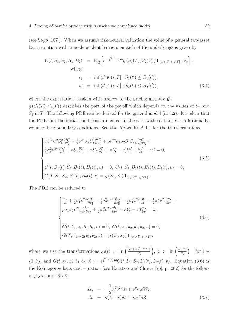
3 Pricing of barrier options within stochastic covariance model 59
(see Sepp [107]). When we assume risk-neutral valuation the value of a general two-asset
barrier option with time-dependent barriers on each of the underlyings is given by
C(t, S1, S2, B1, B2) = EQ
[
e−∫ Tt
r(s)dsg (S1(T ), S2(T ))1ι1>T, ι2>T |Ft
]
,
where
ι1 = inf (t′ ∈ (t, T ] : S1(t′) ≤ B1(t
′)) ,
ι2 = inf (t′ ∈ (t, T ] : S2(t′) ≤ B2(t
′)) , (3.4)
where the expectation is taken with respect to the pricing measure Q.g (S1(T ), S2(T )) describes the part of the payoff which depends on the values of S1 and
S2 in T . The following PDE can be derived for the general model (in 3.2). It is clear that
the PDE and the initial conditions are equal to the case without barriers. Additionally,
we introduce boundary conditions. See also Appendix A.1.1 for the transformations.
12v2νσ2
1S21∂2C∂S2
1+ 1
2v2νσ2
2S22∂2C∂S2
2+ ρv2νσ1σ2S1S2
∂2C∂S1∂S2
+
12σ2vv
2γ ∂2C∂v2
+ rS1∂C∂S1
+ rS2∂C∂S2
+ κ(ζ − v)∂C∂v
+ ∂C∂t− rC = 0,
C(t, B1(t), S2, B1(t), B2(t), v) = 0, C(t, S1, B2(t), B1(t), B2(t), v) = 0,
C(T, S1, S2, B1(t), B2(t), v) = g (S1, S2)1ι1>T, ι2>T.
(3.5)
The PDE can be reduced to
∂G∂t
+ 12σ21v
2ν ∂2G∂x2
1+ 1
2σ22v
2ν ∂2G∂x2
2− 1
2σ21v
2ν ∂G∂x1− 1
2σ22v
2ν ∂G∂x2
+
ρσ1σ2v2ν ∂2G
∂x1∂x2+ 1
2σ2vv
2γ ∂2G∂v2
+ κ(ζ − v)∂G∂v
= 0,
G(t, b1, x2, b1, b2, v) = 0, G(t, x1, b2, b1, b2, v) = 0,
G(T, x1, x2, b1, b2, v) = g (x1, x2)1ι1>T, ι2>T,
(3.6)
where we use the transformations xi(t) := ln
(
Si(t)e∫Tt r(s)ds
Ki
)
, bi := ln(
Bi(T )Ki
)
for i ∈
1, 2, and G(t, x1, x2, b1, b2, v) := e∫ Tt
r(s)dsC(t, S1, S2, B1(t), B2(t), v). Equation (3.6) is
the Kolmogorov backward equation (see Karatzas and Shreve [76], p. 282) for the follow-
ing system of SDEs
dxi = −1
2σ2i v
2νdt+ vνσidWi,
dv = κ(ζ − v)dt+ σvvγdZ, (3.7)

60 3.4 Pricing of two-asset barrier options with Fourier techniques
with r implicitly set to zero.
3.4 Pricing of two-asset barrier options with Fourier
techniques
3.4.1 General pricing formulas for two-asset barrier options
with Fourier techniques
The system in (3.6) can be solved for a group of payoffs and models included in the
general framework (3.2), i.e. for specific values of the parameters γ and ν. A necessary
condition for this group is the existence of an affine and analytic characteristic function
(see Definition 32). A characteristic function, which is regular in a neighbourhood of 0,
is also regular in a strip a < ℑ(u) < b, where a and b are horizontal lines to the real
axis and ℑ(u) describes the imaginary part of u, or in the whole plane, and there it
can be represented by a Fourier integral (see Theorem 14). Thus, for a < ℑ(u) < b the
characteristic function of the process X(t) is identical to the generalized Fourier transform
of the transition density (see Section 2.2.7). Generalized Fourier transforms are inverted
by integrating along a contour in the complex u-plane, parallel to the real axis, with u in
the strip of regularity (see Equation (2.50)). Our work extends Lewis’ approach to two
dimensions (see [81],[82]).
These concepts can be extended to Fourier transforms in two variables.
Theorem 32. (Extension of Theorem 7.1.1 of [84] (see Theorem 14) to R2)
If a characteristic function ϕ(u), where u represents a vector (u1, u2), is regular in a
neighbourhood of the origin, then it is also regular in a horizontal strip to the real axes
and can be represented in this space by a Fourier integral.
Proof.
We follow the lines of Lukacs [84], p. 130ff. Assume that ϕ(u1, u2) is an analytic charac-
teristic function. We know then that all moments of the corresponding distribution exist
and that it admits a MacLaurin expansion
ϕ(u1, u2) =∞∑
k=0
∞∑
k=0
i(k+k)uk1uk2αk,k
k!k!for |u| ≤ c0, (3.8)
where c0 = (c0,1, c0,2) > 0 is the radius of convergence of the series. αk,k =∫
R2 xk1x
k2p(x1, x2)dx1dx2 describes the algebraic moment. This series can be decomposed

3 Pricing of barrier options within stochastic covariance model 61
in an even and an odd part:
even: ϕ1(u1, u2) =1
2(ϕ(u1, u2) + ϕ(−u1,−u2)), (3.9)
odd: ϕ2(u1, u2) =1
2(ϕ(u1, u2)− ϕ(−u1,−u2)). (3.10)
It can be easily seen that
ϕ1(u1, u2) = ϕ11(u1, u2) + ϕ12(u1, u2), (3.11)
ϕ2(u1, u2) = ϕ21(u1, u2) + ϕ22(u1, u2), (3.12)
where
ϕ11(u1, u2) =∞∑
k=0
∞∑
k=0
(−1)k+ku2k1 u2k2 α2k,2k
(2k)!(2k)!, (3.13)
ϕ12(u1, u2) =∞∑
k=1
∞∑
k=1
(−1)k+k−1u2k−11 u2k−1
2 α2k−1,2k−1
(2k− 1)!(2k− 1)!, (3.14)
ϕ21(u1, u2) =∞∑
k=0
∞∑
k=1
i2k+2k−1u2k1 u2k−12 α2k,2k−1
(2k)!(2k − 1)!, (3.15)
ϕ22(u1, u2) =∞∑
k=1
∞∑
k=0
i2k+2k−1u2k−11 u2k2 α2k−1,2k
(2k− 1)!(2k)!. (3.16)
The radii of convergence of these series are denoted by c1, c2, c11, c12, c21, and c22
respectively. From the inequality (derived from the Binomial theorem)
∣∣x2k−1
1 x2k−12
∣∣ ≤ 1
4
(x2k1 + x2k−2
1
) (x2k2 + x2k−2
2
)
=1
4
(x2k1 x
2k2 + x2k1 x
2k−22 + x2k−2
1 x2k2 + x2k−21 x2k−2
2
), (3.17)
it follows that
α2k−1,2k−1
(2k− 1)!(2k − 1)!≤ β2k−1,2k−1
(2k− 1)!(2k − 1)!
≤ 1
4
(α2k,2k
(2k)!(2k)!(2k)(2k) +
α2k,2k−2
(2k)!(2k − 2)!(2k)
+α2k−2,2k
(2k− 2)!(2k)!(2k) +
α2k−2,2k−2
(2k− 2)!(2k − 2)!
)
, (3.18)

62 3.4 Pricing of two-asset barrier options with Fourier techniques
where βk,k =∫
R2 |x1|k |x2|k p(x1, x2)dx1dx2 describes the absolute moment. Thus, c12 ≥c11 ≥ c0, as
limk→∞,k→∞
∣∣∣∣∣∣∣∣∣∣∣∣
(−1)k+k+2u2(k+1)1 u
2(k+1)2 α2(k+1),2(k+1)
(2(k+1))!(2(k+1))!
(−1)k+ku2k1 u2k
2 α2k,2k
(2k)!(2k)!︸ ︷︷ ︸
= 1c11
(2(k+ 1))(2(k + 1))
(2k)(2k)
∣∣∣∣∣∣∣∣∣∣∣∣
=1
c11. (3.19)
We further see that the series∑∞
k=1
∑∞k=1
u2k−11 u2k−1
2 β2k−1,2k−1
(2k−1)!(2k−1)!also converges for |u| < c11.
Now,
∣∣x2k1 x
2k−12
∣∣ ≤ 1
2
(x2k1 x
2k2 + x2k1 x
2k−22
),
and∣∣x2k−1
1 x2k2∣∣ ≤ 1
2
(x2k1 x
2k2 + x2k−2
1 x2k2).
Thus,
α2k,2k−1
(2k)!(2k − 1)!≤ β2k,2k−1
(2k)!(2k − 1)!
≤ 1
2
(α2k,2k
(2k)!(2k)!(2k)(2k) +
α2k,2k−2
(2k)!(2k − 2)!(2k)
)
,
andα2k−1,2k
(2k− 1)!(2k)!≤ β2k−1,2k
(2k− 1)!(2k)!
≤ 1
2
(α2k,2k
(2k)!(2k)!(2k)(2k) +
α2k−2,2k
(2k− 2)!(2k)!(2k)
)
. (3.20)
We derive that c21 ≥ c11 ≥ c0 and c22 ≥ c11 ≥ c0. Thus, c2 ≥ c1. Furthermore, the
series∑∞
k=0
∑∞k=0
uk1u
k2βk,k
(k)!(k)!converges due to β2k,2k = α2k,k as well as (3.18) and (3.20) for
|u| < c11.
Let P be a real vector and denote the radius of convergence of the Taylor series of
ϕ1(u1, u2) (ϕ2) around P by c1(P) (c2(P)). Define the kth derivative with respect to u1
and the kth derivative with respect to u2 with
ϕ(k,k)(u1, u2) = ik+k
∫
R
ei(u1x1+u2x2)xk1xk2p(x1, x2)dx1dx2. (3.21)
3 Pricing of barrier options within stochastic covariance model 63
Note that αk,k = i−(k+k)ϕk,k(0, 0). We see
∣∣ϕ(2k,2k)(P)
∣∣ ≤ α2k,2k and
∣∣ϕ(2k−1,2k−1)(P)
∣∣ ≤ β2k−1,2k−1, (3.22)
∣∣ϕ(2k−1,2k)(P)
∣∣ ≤ β2k−1,2k and
∣∣ϕ(2k,2k−1)(P)
∣∣ ≤ β2k,2k−1. (3.23)
Hence,
c1(P) ≥ c1(0, 0) ≥ c0 and c2(P) ≥ c2(0, 0) ≥ c0, (3.24)
and the Taylor series of ϕ1(u1, u2) and ϕ2(u1, u2) around P converge therefore in circles
of radii at least equal to c0. The same is true for the expansion of ϕ(u1, u2) around P so
that ϕ(u1, u2) is regular at least in the strip |ℑ(u)| ≤ c0.
We have already shown that∑∞
k=0
∑∞k=0
|1|k|2|kβki,k
k!k!converges for || < c0. Thus,
∞∑
k=0
∞∑
k=0
|1|k |2|k βk,kk!k!
≥∞∑
i=0
∞∑
k=0
|1|k |2|kk!k!
∫ A
−A
∫ A
−A
|x1|k |x2|k p(x1, x2)dx1dx2
=
∫ A
−A
∫ A
−A
e|x11|+|2x2|p(x1, x2)dx1dx2, (3.25)
for any A and || < c0. Therefore, the integral∫
R2 ei(u1x1+u2x2)p(x1, x2)dx1dx2, where
u = w + i, is convergent for any || < c0 and any w. This integral is a regular
function in its strip of convergence and agrees with ϕ(u) for real u. Therefore, it must
agree with ϕ(u1, u2) also for complex values u, provided |ℑ(u)| < c0 (see Lukacs [84], p.
131f). The integral converges in a strip a < ℑ(u) < b, where |a| ≥ c0, b ≥ c0 and is
regular inside this strip.
Remark 10. As the moment generating function M(w) is given by M(w) = ϕ(iw) we
can derive from Theorem 32 that if ϕ(u), u = w + i, is regular in a neighbourhood of
the origin the moment generating function exists in a (real) neighbourhood of 0 as long
as is in the strip of convergence of ϕ. Furthermore, there exists a complex analytic
extension M( − iw) to an open set D ⊂ C in the neighbourhood of the origin. See also
[31].
Thus, for a < ℑ(u) < b the characteristic function of the processes X(t) is identical to
the multi-dimensional generalized Fourier transform of the transition density. To apply
these concepts to option pricing we need the following conclusions about the convergence
of the inversion of the Fourier transform of a convolution.
64 3.4 Pricing of two-asset barrier options with Fourier techniques
Theorem 33. (Fourier inversion of a product of functions with ℜ(u) ∈ Rd)
Let f(u) ∈ L1(Rd) be the Fourier transform of a function f(x), f ∈ L1(Rd), and let g(x)
and its Fourier transform g(u) belong to L1(Rd). Then f(u) · g(u) belongs to L1(Rd) and
its Fourier inversion is∫
Rd g(x′)f(x− x′)dx′. The Fourier inversion is defined by
1
(2π)d
∫
Rd
e−i〈x,u〉f(u)g(u)du, (3.26)
where 〈x,u〉 is the scalar product of u and x. If the map x1, x2 →∫
Rd g(x′)f(x − x′)dx′
is continuous the convergence is point-wise.
Proof.
Let g(x) be an integrable function in Rd. The Fourier transform in R
d of g, g, is bounded
by 1
(2π)d2‖g‖1 (see [80], p. 325). Furthermore, we also assume f(u), g(u) ∈ L1. Hence, the
product f g is Lebesgue integrable (see [80], p. 243). Thus,
1
(2π)d
∫
Rd
e−i〈x,u〉f(u)g(u)du =1
(2π)d
∫
Rd
e−i〈x,u〉f(u)
∫
Rd
g(x′)ei〈x′,u〉dx′du
=1
(2π)d
∫
Rd
g(x′)
∫
Rd
e−i〈x−x′,u〉f(u)dudx′
=
∫
Rd
g(x′)f(x− x′)dx′. (3.27)
The inversion is justified by absolute convergence. See also [113], p. 51. If the map
x1, x2 →∫
Rd g(x′)f(x − x′)dx′ is continuous the convergence is point-wise (see [80], p.
327f): Let∫
Rd g(x′)f(x−x′)dx′ be continuous in P0. As (3.26) is valid nearly everywhere
there exists a sequence (Sn) with Sn → P0 in such a way that (3.26) is true in the points
of Sn. The integral in (3.26) is continuous (see [80], p. 282) because the Fourier transform
is a continuous and bounded function. Thus, the identity is also true in P0.
Adding these pieces together we can make the following statement about pricing of barrier
options:
Theorem 34. (Barrier option pricing in R2)
Let us assume
i. the setting described in Equation (3.2),
ii. the existence of an affine analytic characteristic function ϕ(τ,u, z) of the
respective model in the variables z1 := 1√1−ρ2
(
lnS1e
∫Tt r(s)ds
K1−ln
B1(T )K1
σ1− ρz2
)
3 Pricing of barrier options within stochastic covariance model 65
and z2 :=ln
S2e
∫Tt r(s)ds
K2−ln
B2(T )K2
σ2, which is regular in a neighbourhood Sϕ =
u = w + i : ∈ (aϕ, bϕ) , aϕ < 0, bϕ > 0 of the origin, and integrable,
iii. the generalized Fourier transform h(x) of the transformed payoff function
e−c1x1−c2x2g(x) exists in a space Sg = u = w + i : ∈ (ag, bg), is integrable
for |x| <∞, and
iv. ρ = − cos(πn), where n is a natural number and n > 1.
If the space SC ≡ Sϕ ∩ Sg is not empty, then the barrier option value (3.4) is given by
CB (t, S1, S2, B1, B2, v) =ex1c1+x2c2−
∫ Tt
r(s)ds
4π2σ1σ2√
1− ρ2n−1∑
k=0
∫ i2+∞
i2−∞
∫ i1+∞
i1−∞
(
h(u1, u2)
(ϕ(τ,u,−zk, v)− ϕ(τ,u,−zk−), v
)
e(iu1(− b1
σ1
√1−ρ2
+b2ρ
σ2
√1−ρ2
)−iu2b2σ2
))
du1du2, u ∈ SC , (3.28)
where
z(−)k1 = rp cos
(2kπ
n
+
(−) θp)
, z(−)k2 = rp sin
(2kπ
n
+
(−) θp)
,
xi = lnSie
∫ Tt
r(s)ds
Ki
, bi = lnBi(T )
Ki
,
c1 =σ1 − σ2ρ
2σ1(1− ρ2), c2 =
σ2 − σ1ρ2σ2(1− ρ2)
,
h(u1, u2) =
∫ ∞
−∞
∫ +∞
−∞e−x′
1c1−x′2c2g(x′1, x
′2)
e
(iu1
x′1σ1
√1−ρ2
+x′2σ2
(− ρ√1−ρ2
iu1+iu2))
dx′1dx′2, u ∈ Sg,
ϕ(τ,u, z, v) = exp iu1z1 + iu2z2 + V (τ,u, v) ,
where V (τ,u) satisfies the System (3.36). The price converges point-wise if the map
S1, S2 → CB(t, S1, S2, B1, B2, v) is continuous.

66 3.4 Pricing of two-asset barrier options with Fourier techniques
Proof.
We assume the settings described in (3.2) (see Theorem 34, i.). By introducing the
following transformations (see also Appendix A.1.1)
Z(t, x1, x2, b1, b2, v) := e−c1x1−c2x2G(t, x1, x2, b1, b2, v),
c1 :=σ1 − σ2ρ
2σ1(1− ρ2),
c2 :=σ2 − σ1ρ
2σ2(1− ρ2),
we can reduce the PDE problem (3.6) to
∂Z∂t
+ 12σ21v
2ν ∂2Z∂x2
1+ 1
2σ22v
2ν ∂2Z∂x2
2− v2ν σ2
1+σ22−2ρσ1σ2
8(1−ρ2)Z
+ρσ1σ2v2ν ∂2Z
∂x1∂x2+ 1
2σ2vv
2γ ∂2Z∂v2
+ κ(ζ − v)∂Z∂v
= 0,
Z(t, b1, x2, b1, b2, v) = 0, Z(t, x1, b2, b1, b2, v) = 0,
Z(T, x1, x2, b1, b2, v) = e−c1x1−c2x2g(x1, x2)1ι1>T, ι2>T.
(3.29)
The transition probability density function p(t′,x′, v′, t,x, v) is governed by the following
Kolmogorov backward equation and boundary conditions in the backward variables
∂
∂τp(τ, x′1, x
′2, v
′, x1, x2, v) =1
2σ21v
2ν ∂2
∂x21p(τ, x′1, x
′2, v
′, x1, x2, v)
+1
2σ22v
2ν ∂2
∂x22p(τ, x′1, x
′2, v
′, x1, x2, v)
+ρσ1σ2v2ν ∂2
∂x1∂x2p(τ, x′1, x
′2, v
′, x1, x2, v)
−v2ν σ21 + σ2
2 − 2ρσ1σ28(1− ρ2) p(τ, x′1, x
′2, v
′, x1, x2, v)
+1
2σ2vv
2γ ∂2p(τ, x′1, x
′2, v
′, x1, x2, v)
∂v2
+κ(ζ − v)∂p(τ, x′1, x
′2, v
′, x1, x2, v)
∂v, (3.30)
where τ = t′ − t, t′ > t. We apply the following initial and boundary conditions
p(0, x′1, x′2, v
′, x1, x2, v) = δ(x′1 − x1)δ(x′2 − x2)δ(v′ − v),p(τ, x′2, v
′, b1, x2, v) = 0,
p(τ, x′1, x′2, v
′, x1, b2, v) = 0.
3 Pricing of barrier options within stochastic covariance model 67
The payoff of the derivative does not depend on the volatility, therefore we can proceed
with
q(τ,x′,x, v) =
∫ ∞
0
p(τ,x′, v′,x, v)dv′. (3.31)
q solves the Kolmogorov Equation (3.30) (see Definition 38) supplied with the initial and
boundary conditions
q(0, x′1, x′2, x1, x2, v) = δ(x′1 − x1)δ(x′2 − x2),
q(τ, x′1, x′2, b1, x2, v) = 0,
q(τ, x′1, x′2, x1, b2, v) = 0.
In the following we reduce this PDE following the lines of He et al. [64]. We elim-
inate the mixing term by a transformation of coordinates. By using the transforma-
tions z1 := 1√1−ρ2
(x1−b1σ1− ρx2−b2
σ2) and z2 := x2−b2
σ2we map the vertical axis to the line
z2 = −√
1−ρ2
ρz1, while the second (horizontal) boundary is only translated to z2 = 0.
Thus, q(τ, z′1, z′2, z1, z2, v) satisfies the following PDE
∂q
∂τ=
1
2v2ν
∂2q
∂z21+
1
2v2ν
∂2q
∂z22− v2ν σ
21 + σ2
2 − 2ρσ1σ28(1− ρ2) q
+1
2σ2vv
2γ ∂2q
∂v2+ κ(ζ − v)∂q
∂v, (3.32)
with the following initial and boundary conditions
q(0, z′1, z′2, z1, z2, v) = δ(z′1 − z1)δ(z′2 − z2), (3.33)
q(τ, z′1, z′2, z1, 0, v) = 0,
q(τ, z′1, z′2, z1,−
√
1− ρ2ρ
z1, v) = 0. (3.34)
We derive a solution of this PDE for particular values of the correlation, ρ = − cos(πn
)
where n is any natural number (see Theorem 34, iv.). The idea is to find a solution GF
for (3.32) and (3.33) in the whole plane first and restrict it to the actual space (3.34) it
is defined for by using symmetries.
Due to the fact that for certain values of ν and γ the PDE is linear in v, we can guess
affine solutions for GF , i.e. the free space probability density, for those models.
GF (τ, z′1, z′2, z1, z2, v) =
1
4π2
∫ i2+∞
i2−∞
∫ i1+∞
i1−∞exp iu1(z′1 − z1) + iu2(z
′2 − z2)
+V (τ,u, v) du1du2, u = w + i ∈ Sϕ, (3.35)
68 3.4 Pricing of two-asset barrier options with Fourier techniques
where u = (u1, u2) and Sϕ describes a space in a neighbourhood of the origin, parallel to
the real axis, in which the integrand is regular. Inserting (3.35) in (3.32) and (3.33) we
see that V (τ,u, v) has to satisfy the following system.
∂V
∂τ= −1
2v2νu21 −
1
2v2νu22 − v2ν
σ21 + σ2
2 − 2ρσ1σ28(1− ρ2)
+1
2σ2vv
2γ
(
∂2V
∂v2+
(∂V
∂v
)2)
+ κ(ζ − v)∂V∂v
,
V (0,u, v) = 0. (3.36)
Since the process is affine V (τ,u, v) can be denoted by expA0(τ, u) +∑k
i=1Ai(τ, u)vi,
where in the sum Ai(τ, u) are multiplied by v raised to the power of i, i ≤k and (3.36) breaks then down into a system of Riccati equations (see [75]).
This solution is closely related to the concept of characteristic functions: To
see this, we Fourier transform PDE (3.32) and the initial conditions (3.33),
i.e. ϕ(τ,u, v) :=∫∞−∞∫∞−∞ ei(u1z1+u2z2)q(τ, z, v)dz1dz2 or respectively q(τ, z, v) :=
1(2π)2
∫∞−∞∫∞−∞ e−i(u1z1+u2z2)ϕ(τ,u, v)du1du2. Thus, with (A.21) we get
∂ϕ
∂τ= −1
2v2νu21ϕ−
1
2v2νu22ϕ− v2ν
σ21 + σ2
2 − 2ρσ1σ28(1− ρ2) ϕ
+1
2σ2vv
2γ ∂2ϕ
∂v2+ κ(ζ − v)∂ϕ
∂v, (3.37)
with the following initial condition
ϕ(0, u1, u2, v) = eiu1z′1+iu2z
′2 . (3.38)
Inserting
ϕ(τ,u, v) = exp iu1z′1 + iu2z′2 + V (τ,u, v) (3.39)
in Equation (3.37) and initial Condition (3.38) we see that both are satisfied. Thus,
ϕ is the characteristic function of z′1 and z′2. According to Theorem 32 an analytic
characteristic function, which is regular in a neighbourhood of the origin, is also regular
in a horizontal space Sϕ = u = w + i : ∈ (aϕ, bϕ) and can there be represented
by a Fourier integral (see ii.). Hence, in this case ϕ is also the Fourier transform of the
transition density of z1 and z2 (see Theorem 31). The free space solution (3.35) to the
Kolmogorov backward Equation (3.32) can, thus, be interpreted as the Fourier inversion
in the backward variables (z1, z2) of the characteristic function/Fourier transform in the
forward variables (z′1, z′2). G
F is a bounded continuous density if ϕ ∈ L1 (see Theorem 13)
(see ii.), and is, thus, the transition density of z′1, z′2 starting in z1 and z2. The solution
3 Pricing of barrier options within stochastic covariance model 69
for q, satisfying the boundary conditions, can be found from GF using the method of
images as described in [64]. By using the transformations z1 := 1√1−ρ2
(x1−b1σ1− x2−b2
σ2)
and z2 := x2−b2σ2
we mapped the vertical axis to the line z2 = −√
1−ρ2
ρz1, while the first
(horizontal) boundary is translated to z2 = 0. By transforming these to polar coordinates
the vertical boundary is described by the angle tan θp = −√
1−ρ2
ρand the horizontal
boundary by θp = 0. When ρ = − cos(πn
)(see Theorem 34, iv.), the angles take the
special values βp,n = πn; n = 1; 2,. . . For these angles, a method of images solution to the
PDE is possible. Some Gk
G±k (τ, z
′1, z
′2, z1, z2, v) = ±GF (τ, z′1, z
′2, zk1, zk2, v)
satisfy the PDE (3.32) with initial condition for arbitrary zk1, zk2:
G±k (0, z
′1, z
′2, z1, z2, v) = ±δ (z′1 − zk1) δ (z′2 − zk2) .
As the PDE is linear in GF , any linear combination of these G±k ’s, with different
(starting) values of (zk1, zk2) also satisfies the PDE. For the particular solution we take
a combination of n G±k . We have to find this particular solution that also satisfies the
boundary and initial condition.
Consider the case with β = π3, i.e. ρ = −1
2. The first hextant of Figure 3.1 is the
region we want to solve the PDE for, i.e. θp ∈ [0, π3]. In this region a plus symbol is
positioned at P0 = (z01 = rp cos(θp), z02 = rp sin(θp)). This point makes an angle θp with
respect to the z1-axis and is located at a distance rp. Let us denote the lines, which
bound the first hextant by L1 (θp = 0) and L2 (θp = π3). For the other functions we
choose zk1, zk2 at a distance rp from the origin and with the angles θp +2π3, θp +
4π3
and
−θp,−θp + 2π3,−θp + 4π
3. As G+
0 is the only function with (zk1, zk2) positioned in the first
hextant the initial condition is satisfied. We claim that q is given by the combination of
those 6 functions.

70 3.4 Pricing of two-asset barrier options with Fourier techniques
−
P5
+
P2
−
+ P0
P4
P1
−
P3 +
L2
L1
Figure 3.1: Method of images in a circle (with β = π3).
As already seen this combination fulfils the initial condition and it also satisfies the PDE.
Additionally, we know that:
rp cos(+− θp +
2kπ
n) = rp(cos(θp) cos(
2πk
n)
−+ sin(θp) sin(
2πk
n))
= z1 cos(2πk
n)
−+ z2 sin(
2πk
n),
rp sin(+− θp +
2kπ
n) = rp(
+− sin(θp) cos(
2πk
n) + cos(θp) sin(
2πk
n))
=+− z2 cos(
2πk
n) + z1 sin(
2πk
n),
We can see from the symmetry of Figure 3.1 that the functions G±k cancel pairwise
along the solid lines: To obtain zero-value at L1 we add to our first function G+0
the function G−0 with the image point of P0 = (z01, z02) in L1 as starting point:
P1 = (rp cos(−θp), rp sin(−θp)) = (z−01, z−02). For example one can show for any function f
in L1, i.e. θp = 0,
f(z′1 − rp cos(θp), z′2 − rp sin(θp))− f(z′1 − rp cos(−θp), z′2 − rp sin(−θp))= f(z′1 − rp cos(θp), z′2)− f(z′1 − rp cos(θp), z′2)= 0. (3.40)
To balance the point P1 in L2, the solid line with angle β = π3, we add the function G+
1
3 Pricing of barrier options within stochastic covariance model 71
with starting point P2 = (rp cos(θp + 2π3), rp sin(θp + 2π
3)) = (z11, z12).
Furthermore to balance P2 in L1 we add the function G−2 with starting value P3 =
(rp cos(−θp + 4π3), rp sin(−θp + 4π
3)) = (z−11, z
−12) and so on. See [19], p. 277f. Hence,
the boundary conditions are also satisfied, and the combination of the six functions is the
unique solution to the problem.
So in general, we slice a circle in 2n wedges with the same angles βp,n = πn;n = 1; 2, . . .
The first wedge with z01 = rp cos(θp) and z02 = rp sin(θp) always relates to the space
where we want to find a solution to the PDE. For this space the initial condition (3.33) is
satisfied, as z1 = rp cos(θp) and z2 = rp sin(θp). Thus, the combination in fact fulfils the
PDE and the initial condition. So we only need to show that the absorbing conditions
are satisfied. By the symmetry of the wedges in the circle the 2n density functions cancel
along the lines θp = 0 and θp = βp,n in pairs. Thus, the solution is given by
q(τ, x′1, x′2, x1, x2, v) =
n−1∑
k=0
(G+
k (τ, z′1, z
′2, zk1, zk2, v) + G−
k (τ, z′1, z
′2, z
−k1, z
−k2, v)
)
σ1σ2√
1− ρ2,
where 1
σ1σ2
√1−ρ2
is the Jacobi matrix of the transformation from x → z which needs to
be applied if we carry out the integration in the original variable x (see Theorem 31),
G±k (τ, z
′1, z
′2, z
(−)k1 , z
(−)k2 , v) =
+
(−) GF(τ, z′1, z
′2, z1 = zk1
(−), z2 = zk2(−), v
),
zk1(−) = rp cos
(2kπ
n
+
(−) θp)
, zk2(−) = rp sin
(2kπ
n
+
(−) θp)
,
rp =√
z21 + z22 , tan θp =z2z1,
z1 =1
√
1− ρ2
[x1 − b1σ1
− ρ(x2 − b2σ2
)]
= z01, z2 =x2 − b2σ2
= z02. (3.41)
72 3.4 Pricing of two-asset barrier options with Fourier techniques
From risk-neutral pricing, it follows
CB (t, S1, S2, B1, B2, v) = ex1c1+x2c2−∫ Tt
r(s)ds
∫ ∞
−∞
∫ ∞
−∞
(
e−x′1c1−x′
2c2g(x′1, x′2)
q(τ, x′1, x′2, v, x1, x2)
)
dx′1dx′2
(3.41)=
ex1c1+x2c2−∫ Tt
r(s)ds
4π2σ1σ2√
1− ρ2∫ ∞
−∞
∫ ∞
−∞e−x′
1c1−x′2c2g(x′1, x
′2)
n−1∑
k=0
∫ i2+∞
i2−∞
∫ i1+∞
i1−∞
(
ϕ(τ,u, z′ − zk, v)
−ϕ(τ,u, z′ − zk−, v)
)
du1du2dx′1dx
′2. (3.42)
We have required that the payoff function and the characteristic function are Lebesgue
integrable in the generalized sense in a space SC (see ii. and iii.). Moreover, we know
that the transformed payoff function is Lebesgue integrable (see iii.). Hence, g(x′1, x′2) is
bounded and the integrand is Lebesgue integrable (see [80], p. 243), and we can apply
Fubini’s theorem and change the sum and integrals if there exists a space SC = Sϕ ∩ Sg.
Then, the above expression can be simplified. We denote the Fourier transform of the
complete payoff function by h(u1, u2)
h(u1, u2) =
∫ ∞
−∞
∫ +∞
−∞e−x′
1c1−x′2c2g(x′1, x
′2)
e
(iu1
x′1σ1
√1−ρ2
+x′2σ2
(− ρ√1−ρ2
iu1+iu2))
dx′1dx′2, u ∈ Sg. (3.43)
Then, using (3.39) and (3.35),
CB (t, S1, S2, B1, B2, v) =ex1c1+x2c2−
∫ Tt
r(s)ds
4π2σ1σ2√
1− ρ2n−1∑
k=0
∫ i2+∞
i2−∞
∫ i1+∞
i1−∞
(
h(u1, u2)
(ϕ(τ,u,−zk, v)− ϕ(τ,u,−zk−, v)
)(3.44)
e(iu1(− b1
σ1
√1−ρ2
+b2ρ
σ2
√1−ρ2
)−iu2b2σ2
))
du1du2,
u ∈ SC = Sϕ ∩ Sg.
According to Theorem 33 together with (ii. and iii.) CB(t, S1, S2, B1, B2, v) converges
point-wise to the actual solution if the function S1, S2 → CB (t, S1, S2, B1, B2, v) is con-
tinuous in S1 and S2.
3 Pricing of barrier options within stochastic covariance model 73
Remark 11. We know that
q(τ, x′1 − x1, x′2 − x2, v) =1
4π2σ1σ2√
1− ρ2n−1∑
k=0
∫ i2+∞
i2−∞
∫ i1+∞
i1−∞eiu1z
′1+iu2z
′2
(ϕ(τ,u,−zk, v)− ϕ(τ,u,−zk−, v)
)du1du2, (3.45)
and (3.43). Hence, (3.44) can be transformed to
CB (t, S1, S2, B1, B2, v) =ex1c1+x2c2−
∫ Tt
r(s)ds
4π2σ1σ2√
1− ρ2n−1∑
k=0
∫ i2+∞
i2−∞
∫ i1+∞
i1−∞(∫ ∞
−∞
∫ ∞
−∞(e−c1x
′1−c2x
′2g(x′1, x
′2)e
iu1z′1+iu2z
′2dx′1dx
′2)
(ϕ(τ,u,−zk, v)− ϕ(τ,u,−zk−, v)
))
du1du2
=ex1c1+x2c2−
∫ Tt
r(s)ds
4π2σ1σ2√
1− ρ2n−1∑
k=0
∫ ∞
−∞
∫ ∞
−∞e−c1x
′1−c2x
′2g(x′1, x
′2)
∫ i2+∞
i2−∞
∫ i1+∞
i1−∞eiu1z
′1+iu2z
′2
(ϕ(τ,u,−zk, v)− ϕ(τ,u,−zk−, v))du1du2dx′1dx′2= ex1c1+x2c2−
∫ Tt
r(s)ds (3.46)∫ ∞
−∞
∫ ∞
−∞e−c1x
′1−c2x
′2g(x′1, x
′2)q(τ, x
′1 − x1, x′2 − x2, v)dx′1dx′2.
3.4.2 Properties of selected two-dimensional affine characteris-
tic functions
In this section we want to treat properties of two characteristic functions which are
included in the general set-up of (3.2) and which fulfil the PDE (3.37), i.e. have an
affine characteristic function. The first one is a Heston-type characteristic function with
γ = ν = 12, the other model, in which the covariance is governed by an Ornstein-Uhlenbeck
process, has actually no affine characteristics for (Si, v), however, a characteristic function
can be derived (see Kallsen [75]). In the following we analyse properties like the regular-
ity at the origin in Sϕ and integrability in this space for the Heston- and the Stein and
Stein-type two-dimensional models.
Proposition 2. (Heston-type characteristic function)
The Heston-type characteristic function is defined by
ϕH(τ,u) = exp
iu1z1 + iu2z2 +1
σ2v
(AH(τ,u) + BH(τ,u)v)
, (3.47)
74 3.4 Pricing of two-asset barrier options with Fourier techniques
where
BH(τ,u) =(κ− d) (1− exp (−dτ))
1− κ−dκ+d
exp (−dτ)
=
(
κ− dsinh
(d2τ)+ κ
dcosh
(d2τ)
cosh(d2τ)+ κ
dsinh
(d2τ)
)
, (3.48)
AH(τ,u) = ζκ
(
(κ− d) τ − 2 ln(1− κ−d
κ+dexp (−dτ)
1− κ−dκ+d
))
= κζ
(
κτ − 2 ln
(κ
dsinh
(d
2τ
)
+ cosh
(d
2τ
)))
, (3.49)
d = d(u) =
√
κ2 + σ2v
(
u2 +σ21 + σ2
2 − 2ρσ1σ24(1− ρ2)
)
, (3.50)
where u2 = u21+u22. For
4κ2
ǫ2> −σ2
1+σ22−2ρσ1σ2
1−ρ2the characteristic function, ϕH , is integrable
and regular in a neighborhood of the origin [w−,w+] with w−1 < 0 < w+
1 (w−2 < 0 < w+
2
respectively).
Proof.
For the derivation of the characteristic function see Appendix A.1.2. For the analysis of
the regularity in a space SϕHin the neighbourhood of the origin we follow the lines of del
Bano Rollin et al. [31]. Define D(u) = d(u)2. If we assume that 4κ2
σ2v> −σ2
1+σ22−2ρσ1σ2
1−ρ2,
we see that ϕH is well-defined and regular in a neighbourhood of the origin according
to Cauchy’s integral theorem (see Theorem 15), i.e. according to Remark 10 the moment
generating function M() exists in a (real) neighbourhood of 0 and there exists a complex
analytic extension of MH(w) = ϕ(iw) to an open set D ⊂ C in the neighbourhood of
the origin. Observing the components of the moment generating function we see that the
main and most critical ingredient of the moment generating function is
f(w) =κ
d(w)sinh
(d(w)
2τ
)
+ cosh
(d(w)
2τ
)
, (3.51)
with
d(w)2 = d(iw)2 = D(−w) = κ2 + σ2v
(
−w21 − w2
2 +σ21 + σ2
2 − 2ρσ1σ24(1− ρ2)
)
, (3.52)
because this part is in the denominator of BH and in the log-part of AH . D(w) with
w ∈ R2 is a cup-shaped inverted parabola with leading coefficient −σ2
v and real roots
3 Pricing of barrier options within stochastic covariance model 75
w−1 < 0 < w+
1 (w−2 < 0 < w+
2 respectively) given by
w±1,2 = ±
√
σ21 + σ2
2 − 2ρσ1σ24(1− ρ2) +
κ2
σ2v
, (3.53)
i.e. d(w) ≥ 0 on [w−,w+]. Hence, f(z) is well-defined and analytic in such an interval.
As f has no zeroes in [w−,w+] the moment generating function exists there. We define
DefH(z) =w ∈ R
2 :MH(w) = E[e〈wz〉] <∞
. (3.54)
And thus, [w−,w+] ⊂ DefH(z) and SϕH= u = w + i : ∈ (aϕH
, bϕH), where aϕH
=
w− and bϕH= w+. Please note that E (ez1+z2) might not exist. We prove integrability of
the characteristic function ϕH(w+ i) with u = w+ i ⊂ SϕH. It suffices to show that
the real part of the exponent decays like |w| (see [38]). In the following the real part of x is
denoted ℜ(x). The real part of a square root in R2 is given by ℜ(
√w + i) =
√|w+i|+w
2
(see [1], 3.7.27). Thus, for −ℜ(d) we see
−ℜ(d) = − 1√2
(∣∣∣κ2 + (w2
1 + w22)σ
2v − (2
1 +22)σ
2v + 2iw11σ
2v + 2iw22σ
2v
+σ2v
σ1 + σ2 − 2ρσ1σ24(1− ρ2)
∣∣∣
+κ2 + (w21 + w2
2)σ2v − (2
1 +22)σ
2v + σ2
v
σ1 + σ2 − 2ρσ1σ24(1− ρ2)
) 12
≤ − 1√2
√
κ2 + (w21 + w2
2)σ2v − (2
1 +22)σ
2v + σ2
v
σ1 + σ2 − 2ρσ1σ24(1− ρ2)
≤ − c√2|w| σv, (3.55)
where c is a constant. Next, we take a closer look at the real part of BH . Note that as
long as κ < d (which is always the case for w → ∞ the denominator of the fraction is
bigger than the nominator. The fraction, however, approaches 1 as w grows due to the
graphs of the cosh- and sinh- functions. Thus, we find
−ℜ(
dsinh
(d2τ)+ κ
dcosh
(d2τ)
cosh(d2τ)+ κ
dsinh
(d2τ)
)
≤ − c1√2|w| σv, (3.56)
76 3.4 Pricing of two-asset barrier options with Fourier techniques
where c1 is a constant. Another important ingredient is the log part. The following is
true as w1 and w2 increase, i.e. we can assume κ < d:
ℜ(
−2 ln(κ
dsinh
(d
2τ
)
+ cosh
(d
2τ
)))
≤ ℜ(
−2 ln(
ed
2τ))
≤ − cτ√2|w| σv. (3.57)
Hence, the exponent decays component-wise like |w| and the characteristic function is
integrable in the space SϕH.
Proposition 3. (Stein and Stein-type characteristic function)
The Stein and Stein-type characteristic function is defined by
ϕS2(τ,u) = exp
iu1z1 + iu2z2 +1
σ2v
(AS2(τ,u) + BS2(τ,u)v + CS2(τ,u)v
2)
, (3.58)
where
CS2(τ,u) =1
2
(
κ− dsinh (dτ) + κ
dcosh (dτ)
cosh (dτ) + κdsinh (dτ)
)
, (3.59)
BS2(τ,u) =1
d
(
κζd− κ3ζ
d
)
+ κ2ζ(sinh (dτ) + κ
dcosh (dτ)
)
cosh (dτ) + κdsinh (dτ)
− κζd
, (3.60)
AS2(τ,u) = −σ2v
2ln(
cosh (dτ) +κ
dsinh (dτ)
)
+σ2v
2κτ
+κ2ζ2d2 − κ4ζ2
2d3
(sinh (dτ)
cosh (dτ) + κdsinh (dτ)
− dτ
)
+κ2ζ
(
κζd− κ3ζ
d
)
d3(
cosh(dτ)− 1
cosh (dτ) + κdsinh (dτ)
), (3.61)
with d(u) given in (3.50). For 4κ2
ǫ2> −σ2
1+σ22−2ρσ1σ2
1−ρ2the characteristic function, ϕH ,
is integrable and regular in a neighborhood of the origin [w−,w+] with w−1 < 0 < w+
1
(w−2 < 0 < w+
2 respectively).
Proof.
For a proof of the characteristic function see Appendix A.1.2. We proceed analogously
to before with the analysis of the regularity in a space Sϕ in the neighbourhood of the
origin. Again, if we assume that 4κ2
σ2v> −σ2
1+σ22−2ρσ1σ2
1−ρ2, we see that ϕ is well-defined and
regular in a neighbourhood of the origin. The main ingredient of the moment generating
3 Pricing of barrier options within stochastic covariance model 77
function is
f(w) =κ
d(w)sinh
(d(w)
2τ
)
+ cosh
(d(w)
2τ
)
. (3.62)
Thus, we can transfer the results from above and conclude that [w−,w+] ⊂ DefS2(z)
and SϕS2= u = w + i : ∈ (aϕS2
, bϕS2), where aϕS2
= w− and bϕS2= w+. With
respect to the integrability we can see that ϕS2 is composed of similar expressions as ϕH .
Performing similar techniques one can easily see that the exponent decays like |w| andthe characteristic function is integrable in the space SϕS2
.
Remark 12. If the three-factor model degenerates to a two-factor GBM model then the
characteristic function is given by
ϕGBM(u) = e
(
iu1z1+iu2z2− 12τ
(
u21+u2
2+(σ21+σ2
2−2ρσ1σ24(1−ρ2)
)
))
. (3.63)
Proof.
For κ, ζ, σv → 0, v(0)→ 1 we can show that the three-factor stochastic volatility Heston-
type and the Stein and Stein-type model degenerate to the two-factor geometric Brownian
motion model. First, we take the limits of AH(τ,u), BH(τ,u), AS2(τ,u), BS2(τ,u), and
CS2(τ,u) when κ, ζ, σv → 0, v(0)→ 1:
limκ,σv ,ζ→0,v(0)→1
AH(τ,u)
σ2v
= 0,
limκ,σv ,ζ→0,v(0)→1
BH(τ,u)v(0)
σ2v
= limκ,σv ,ζ→0,v(0)→1
1
σ2v
(κ2 − d2) (1− exp (−dτ))(κ+ d)− (κ− d) exp (−dτ)
= limκ,σv ,ζ→0,v(0)→1
−
(
u21 + u22 +σ21+σ2
2−2ρσ1σ2
4(1−ρ2)
)
(1− 1 + dτ)
(κ+ d)− (κ− d) (1− dτ)
= limκ,σv ,ζ→0,v(0)→1
−
(
u21 + u22 +σ21+σ2
2−2ρσ1σ2
4(1−ρ2)
)
dτ
2d+ dτ (κ− d)
= −
(
u21 + u22 +σ21+σ2
2−2ρσ1σ2
4(1−ρ2)
)
τ
2,
limκ,σv ,ζ→0,v(0)→1
AS2(τ,u)
σ2v
= 0,
limκ,σv ,ζ→0,v(0)→1
BS2(τ,u)v(0)
σ2v
= 0,
limκ,σv ,ζ→0,v(0)→1
CS2(τ,u)v(0)2
σ2v
= −
(
u21 + u22 +σ21+σ2
2−2ρσ1σ2
4(1−ρ2)
)
τ
2,
78 3.4 Pricing of two-asset barrier options with Fourier techniques
where the limit of CS2v(0)2
σ2v
is calculated analogously to the limes of BHv(0)σ2v
. Thus, both
characteristic functions, ϕH(τ,u) ϕS2(τ,u), approach in the limit
limκ,σv ,ζ→0,v(0)→1
ϕH,S2(u) = eiu1z1+iu2z2−
(
u21+u22+σ21+σ2
2−2ρσ1σ24(1−ρ2)
)
τ
2 . (3.64)
It can be shown that this limit is consistent with the characteristic function of the two-
factor GBM model. The characteristic function of the GBM model satisfies the following
PDE
∂q
∂τ=
1
2
∂2q
∂z21+
1
2
∂2q
∂z22− σ2
1 + σ22 − 2ρσ1σ2
8(1− ρ2) q, (3.65)
with the initial condition ϕGBM(0,u) = eiu1z1+iu2z2 . It can be easily seen that (3.64)
satisfies the terminal condition and also (3.65).
This function is obviously regular in the whole space, and the moment-generating function
exists everywhere. Furthermore, it is integrable in the whole space.
3.4.3 Pricing of two-asset double-digital options with Fourier
techniques
Double-digital options pay out one unit provided that both underlyings are at maturity
time T above their predefined strike price K1 and K2. In the case of a double-digital
barrier option the payout is only guaranteed if both underlyings do not cross the given
barriers B1(t) = B1e∫ t0 r(s)ds and B2(t) = B2e
∫ t0 r(s)ds during the lifetime of the option.
The value of a digital option with time-dependent barriers on each of the underlyings is
given as the expectation of two discounted indicator functions:
C2D(t, S1, S2, B1, B2) = EQ[e−
∫ Tt
r(s)ds1S1(T )>K1, S2(T )>K2
1ι1>T, ι2>T |Ft
], (3.66)
where
ι1 = inf (t′ ∈ (t, T ] : S1(t′) ≤ B1(t
′)) ,
ι2 = inf (t′ ∈ (t, T ] : S2(t′) ≤ B2(t
′)) .
Thus, we have to Fourier transform e−c1x1−c2x2gD(x1, x2) = e−c1x1−c2x21x1(T )>0 ∧ x2(T )>0.
For c1, c2 < 0 the integrals are unbounded and e−c1x1−c2x2gD does not belong to L1. Thus,
the Fourier transform does not exist (see also Schmelzle [104] for a summary). This could
be circumvented by introducing a damping factor like in Carr and Madan [18], Dempster

3 Pricing of barrier options within stochastic covariance model 79
and Hong [33], or Eberlein et al. [38]. The introduction of a damping factor has the same
effect as the generalized Fourier transform along a contour in the complex space, parallel
to the real axis, i.e. loosely speaking it renders an actual non-Lebesgue integrable payoff
integrable (see also [82] and [104]):
hD(u1, u2) =
∫ ∞
0
∫ ∞
0
e−x′1c1−x′
2c2e
(
iu1x′1
σ1
√1−ρ2
+x′2σ2
(
− ρ√1−ρ2
iu1+iu2
))
dx′1dx′2
=1
i u1
σ1
√1−ρ2− c1
1
i
(
u2
σ2− ρu1
σ2
√1−ρ2
)
− c2. (3.67)
The integral only exists if u ∈ SgD =
u = w + i : 1 > −c1σ1√
1− ρ2∧2 >
ρ√1−ρ2
1 − c2σ2 . The same payoff function dampened by e−αd1z
′1−αd
2z′2 , where z′1
and z′2 are given in 3.41, can also be transformed
h∗D(u1, u2) =
∫ ∞
0
∫ ∞
0
e−αd
1
x′1σ1
√1−ρ2
− x′2σ2
(
− ρ√1−ρ2
αd1+αd
2
)
e−x′1c1−x′
2c2
e
(
iu1x′1
σ1
√1−ρ2
+x′2σ2
(− ρ√1−ρ2
iu1+iu2)
)
dx′1dx′2
=1
i u1
σ1
√1−ρ2− αd
1
σ1
√1−ρ2− c1
1
i
(
u2
σ2− ρu1
σ2
√1−ρ2
)
+ραd
1
σ2
√1−ρ2− αd
2
σ2− c2
,
where we have to choose αdi accordingly with α
d1 > −c1σ1
√
1− ρ2 and αd2 >
ρ√1−ρ2
αd1−c2σ2
assuming u real. In Section 3.4.5 we show one of the possibilities to derive the price of the
derivative with the dampened payoff function. The price of the option in the generalized
Fourier framework can be given in the following corollary.
Corollary 4. (Double-digital barrier option price)
Let us assume
i. the setting described in Equation (3.2),
ii. the existence of an affine analytic characteristic function ϕ(τ,u, z), which is regular
in a neighbourhood Sϕ = u = w + i : ∈ (aϕ, bϕ) , aϕ < 0, bϕ > 0 of the
origin, and integrable,
iii. that the generalized Fourier transform hD(x) of the transformed payoff function
e−c1x1−c2x2gD(x)1ι1>T,ι2>T exists in a space SgD = u = w + i :
1 > −c1σ1√
1− ρ2 ∧2 >ρ√1−ρ2
1 − c2σ2 , is there integrable for |x| <∞, and
iv. ρ = − cos(πn), where n is a natural number and n > 1.
80 3.4 Pricing of two-asset barrier options with Fourier techniques
If the space SCD≡ Sϕ ∩ SgD is not empty, the double-digital barrier option value is given
by
C2D (t, S1, S2, B1, B2, v) =ex1c1+x2c2−
∫ Tt
r(s)ds
4π2σ1σ2√
1− ρ2n−1∑
k=0
∫ i2+∞
i2−∞
∫ i1+∞
i1−∞hD(u)
(ϕ(τ,u,−zk, v)− ϕ(τ,u,−zk−, v)
)(3.68)
e(iu1(− b1
σ1
√1−ρ2
+b2ρ
σ2
√1−ρ2
)−iu2b2σ2
)du1du2, u ∈ SCD
,
where ϕ, z(−)i , xi, bi, and ci are given in Theorem 34. hD(u1, u2) is indicated in (3.67).
The corollary directly follows from Theorem 34 and Equation (3.67). Note that if ρ < 0,
c1, c2 > 0. Thus, in those cases we can choose = 0, i.e. we integrate on the real space.
By using the method of images in the plane we can derive prices for double-digitals with a
barrier on S2 only: C1D(t, S1, S2, B2) = EQ[e−
∫ Tt
r(s)ds1S1(T )>K1 ∧ S2(T )>K21ι2>T |Ft
].
The solution is found by reflecting the characteristic function in the plane (z2(0) →−z2(0)).
Corollary 5. (Double-digital single-barrier option price)
Let us assume the setting described in Equation (3.2) and the assumptions of Corollary
4, then the double-digital single-barrier (in S2) option value is given for any ρ by
C1D(t, S1, S2, B2, v) =ex1c1+x2c2−
∫ Tt
r(s)ds
4π2σ1σ2√
1− ρ2∫ i2+∞
i2−∞
∫ i1+∞
i1−∞hD(u)
(ϕ(τ,u,−z1,−z2, v)− ϕ(τ,u,−z1, z2, v)) (3.69)
e
(
iu1b2ρ
σ2
√1−ρ2
−iu2b2σ2
)
du1du2, u ∈ SCD,
where ϕ, xi, b2, ci, are given in Theorem 34, and hD(u1, u2) is given in (3.67).
The corollary directly follows from Theorem 34 and Equation (3.67). For details on the
method of images in a half-space please refer to Appendix A.1.3.
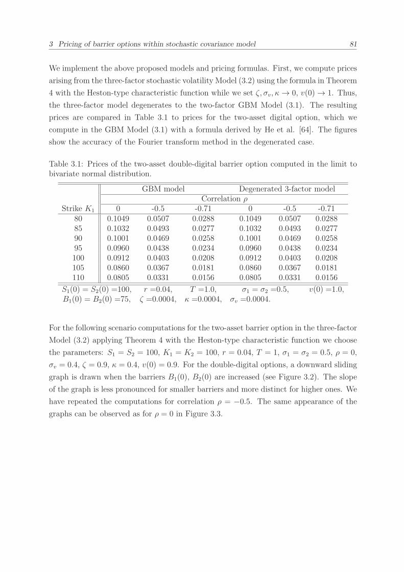
3 Pricing of barrier options within stochastic covariance model 81
We implement the above proposed models and pricing formulas. First, we compute prices
arising from the three-factor stochastic volatility Model (3.2) using the formula in Theorem
4 with the Heston-type characteristic function while we set ζ, σv, κ→ 0, v(0)→ 1. Thus,
the three-factor model degenerates to the two-factor GBM Model (3.1). The resulting
prices are compared in Table 3.1 to prices for the two-asset digital option, which we
compute in the GBM Model (3.1) with a formula derived by He et al. [64]. The figures
show the accuracy of the Fourier transform method in the degenerated case.
Table 3.1: Prices of the two-asset double-digital barrier option computed in the limit tobivariate normal distribution.
GBM model Degenerated 3-factor modelCorrelation ρ
Strike K1 0 -0.5 -0.71 0 -0.5 -0.7180 0.1049 0.0507 0.0288 0.1049 0.0507 0.028885 0.1032 0.0493 0.0277 0.1032 0.0493 0.027790 0.1001 0.0469 0.0258 0.1001 0.0469 0.025895 0.0960 0.0438 0.0234 0.0960 0.0438 0.0234100 0.0912 0.0403 0.0208 0.0912 0.0403 0.0208105 0.0860 0.0367 0.0181 0.0860 0.0367 0.0181110 0.0805 0.0331 0.0156 0.0805 0.0331 0.0156
S1(0) = S2(0) =100, r =0.04, T =1.0, σ1 = σ2 =0.5, v(0) =1.0,B1(0) = B2(0) =75, ζ =0.0004, κ =0.0004, σv =0.0004.
For the following scenario computations for the two-asset barrier option in the three-factor
Model (3.2) applying Theorem 4 with the Heston-type characteristic function we choose
the parameters: S1 = S2 = 100, K1 = K2 = 100, r = 0.04, T = 1, σ1 = σ2 = 0.5, ρ = 0,
σv = 0.4, ζ = 0.9, κ = 0.4, v(0) = 0.9. For the double-digital options, a downward sliding
graph is drawn when the barriers B1(0), B2(0) are increased (see Figure 3.2). The slope
of the graph is less pronounced for smaller barriers and more distinct for higher ones. We
have repeated the computations for correlation ρ = −0.5. The same appearance of the
graphs can be observed as for ρ = 0 in Figure 3.3.
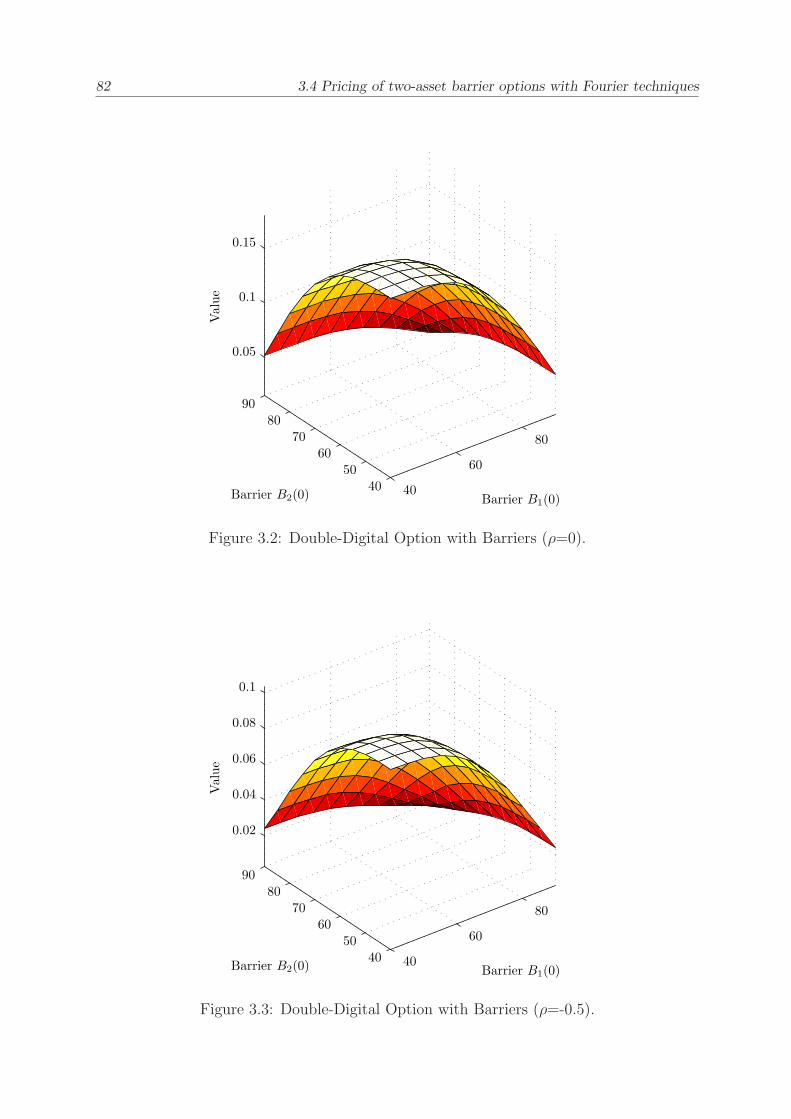
82 3.4 Pricing of two-asset barrier options with Fourier techniques
Value
Barrier B2(0) Barrier B1(0)40
60
80
4050
6070
8090
0.05
0.1
0.15
Figure 3.2: Double-Digital Option with Barriers (ρ=0).
Value
Barrier B2(0) Barrier B1(0)40
60
80
4050
6070
8090
0.02
0.04
0.06
0.08
0.1
Figure 3.3: Double-Digital Option with Barriers (ρ=-0.5).
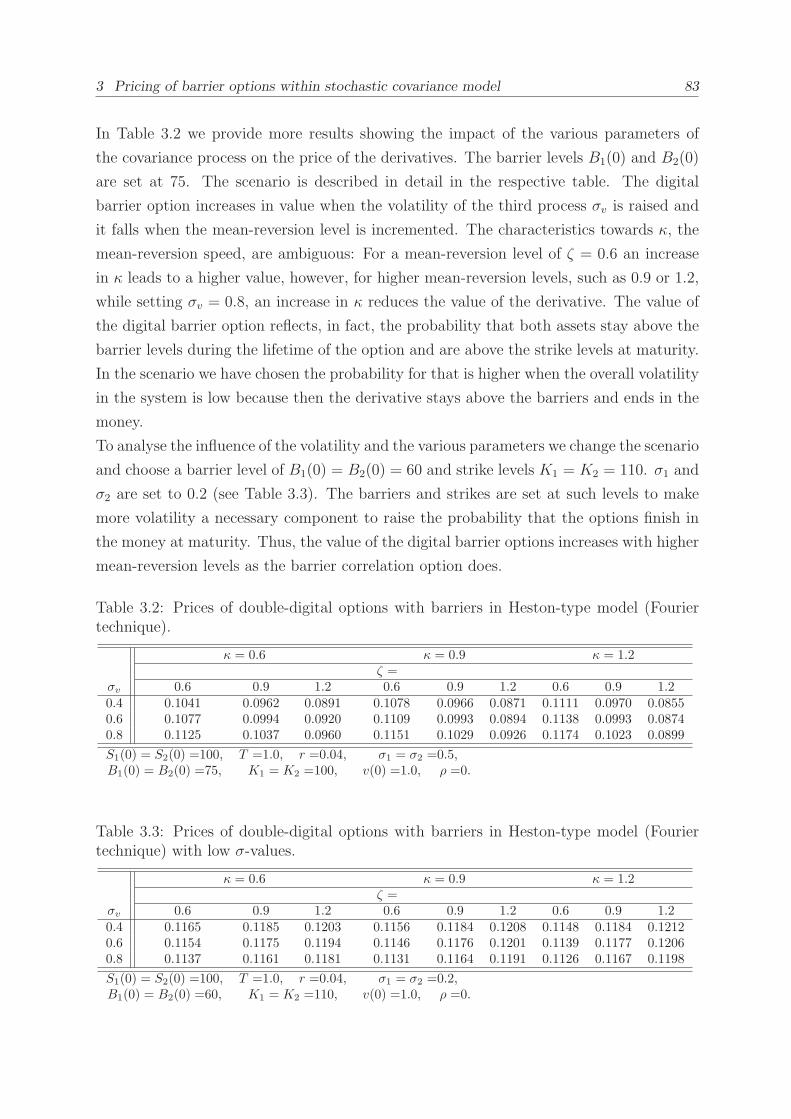
3 Pricing of barrier options within stochastic covariance model 83
In Table 3.2 we provide more results showing the impact of the various parameters of
the covariance process on the price of the derivatives. The barrier levels B1(0) and B2(0)
are set at 75. The scenario is described in detail in the respective table. The digital
barrier option increases in value when the volatility of the third process σv is raised and
it falls when the mean-reversion level is incremented. The characteristics towards κ, the
mean-reversion speed, are ambiguous: For a mean-reversion level of ζ = 0.6 an increase
in κ leads to a higher value, however, for higher mean-reversion levels, such as 0.9 or 1.2,
while setting σv = 0.8, an increase in κ reduces the value of the derivative. The value of
the digital barrier option reflects, in fact, the probability that both assets stay above the
barrier levels during the lifetime of the option and are above the strike levels at maturity.
In the scenario we have chosen the probability for that is higher when the overall volatility
in the system is low because then the derivative stays above the barriers and ends in the
money.
To analyse the influence of the volatility and the various parameters we change the scenario
and choose a barrier level of B1(0) = B2(0) = 60 and strike levels K1 = K2 = 110. σ1 and
σ2 are set to 0.2 (see Table 3.3). The barriers and strikes are set at such levels to make
more volatility a necessary component to raise the probability that the options finish in
the money at maturity. Thus, the value of the digital barrier options increases with higher
mean-reversion levels as the barrier correlation option does.
Table 3.2: Prices of double-digital options with barriers in Heston-type model (Fouriertechnique).
κ = 0.6 κ = 0.9 κ = 1.2ζ =
σv 0.6 0.9 1.2 0.6 0.9 1.2 0.6 0.9 1.20.4 0.1041 0.0962 0.0891 0.1078 0.0966 0.0871 0.1111 0.0970 0.08550.6 0.1077 0.0994 0.0920 0.1109 0.0993 0.0894 0.1138 0.0993 0.08740.8 0.1125 0.1037 0.0960 0.1151 0.1029 0.0926 0.1174 0.1023 0.0899
S1(0) = S2(0) =100, T =1.0, r =0.04, σ1 = σ2 =0.5,B1(0) = B2(0) =75, K1 = K2 =100, v(0) =1.0, ρ =0.
Table 3.3: Prices of double-digital options with barriers in Heston-type model (Fouriertechnique) with low σ-values.
κ = 0.6 κ = 0.9 κ = 1.2ζ =
σv 0.6 0.9 1.2 0.6 0.9 1.2 0.6 0.9 1.20.4 0.1165 0.1185 0.1203 0.1156 0.1184 0.1208 0.1148 0.1184 0.12120.6 0.1154 0.1175 0.1194 0.1146 0.1176 0.1201 0.1139 0.1177 0.12060.8 0.1137 0.1161 0.1181 0.1131 0.1164 0.1191 0.1126 0.1167 0.1198
S1(0) = S2(0) =100, T =1.0, r =0.04, σ1 = σ2 =0.2,B1(0) = B2(0) =60, K1 = K2 =110, v(0) =1.0, ρ =0.
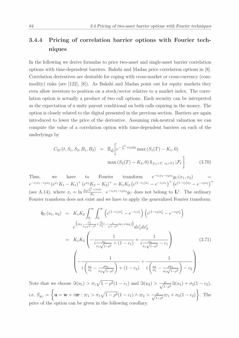
84 3.4 Pricing of two-asset barrier options with Fourier techniques
3.4.4 Pricing of correlation barrier options with Fourier tech-
niques
In the following we derive formulas to price two-asset and single-asset barrier correlation
options with time-dependent barriers. Bakshi and Madan price correlation options in [8].
Correlation derivatives are desirable for coping with cross-market or cross-currency (com-
modity) risks (see [122], [8]). As Bakshi and Madan point out for equity markets they
even allow investors to position on a stock/sector relative to a market index. The corre-
lation option is actually a product of two call options. Each security can be interpreted
as the expectation of a unity payout conditional on both calls expiring in the money. The
option is closely related to the digital presented in the previous section. Barriers are again
introduced to lower the price of the derivative. Assuming risk-neutral valuation we can
compute the value of a correlation option with time-dependent barriers on each of the
underlyings by
C2C(t, S1, S2, B1, B2) = EQ
[
e−∫ Tt
r(s)dsmax (S1(T )−K1, 0)
max (S2(T )−K2, 0)1ι1>T, ι2>T |Ft
]
. (3.70)
Thus, we have to Fourier transform e−c1x1−c2x2gC(x1, x2) =
e−c1x1−c2x2 (ex1K1 −K1)+ (ex2K2 −K2)
+ = K1K2
(e(1−c1)x1 − e−c1x1
)+ (e(1−c2)x2 − e−c2x2
)+
(see A.14), where xi = ln Sie∫Tt r(s)ds
Ki. e−c1x1−c2x2gC does not belong to L1. The ordinary
Fourier transform does not exist and we have to apply the generalized Fourier transform:
hC(u1, u2) = K1K2
∫ ∞
0
∫ ∞
0
(
e(1−c1)x′1 − e−c1x
′1
)(
e(1−c2)x′2 − e−c2x
′2
)
e
(iu1
x′1σ1
√1−ρ2
+x′2σ2
(− ρ√1−ρ2
iu1+iu2))
dx′1dx′2
= K1K2
− 1
i u1
σ1
√1−ρ2
+ (1− c1)+
1
i u1
σ1
√1−ρ2− c1
(3.71)
− 1
i
(
u2
σ2− ρu1
σ2
√1−ρ2
)
+ (1− c2)+
1
i
(
u2
σ2− ρu1
σ2
√1−ρ2
)
− c2
.
Note that we choose ℑ(u1) > σ1√
1− ρ2(1 − c1) and ℑ(u2) > ρ√1−ρ2ℑ(u1) + σ2(1 − c2),
i.e. SgC =
u = w + i : 1 > σ1√
1− ρ2(1− c1) ∧2 >ρ√1−ρ2
1 + σ2(1− c2)
. The
price of the option can be given in the following corollary.
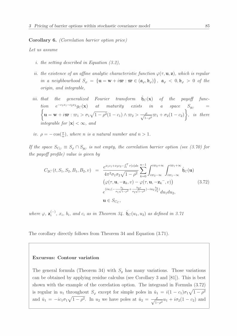
3 Pricing of barrier options within stochastic covariance model 85
Corollary 6. (Correlation barrier option price)
Let us assume
i. the setting described in Equation (3.2),
ii. the existence of an affine analytic characteristic function ϕ(τ,u, z), which is regular
in a neighbourhood Sϕ = u = w + i : ∈ (aϕ, bϕ) , aϕ < 0, bϕ > 0 of the
origin, and integrable,
iii. that the generalized Fourier transform hC(x) of the payoff func-
tion e−c1x1−c2x2gC(x) at maturity exists in a space SgC =
u = w + i : 1 > σ1√
1− ρ2(1− c1) ∧2 >ρ√1−ρ2
1 + σ2(1− c2)
, is there
integrable for |x| <∞, and
iv. ρ = − cos(πn), where n is a natural number and n > 1.
If the space SCC≡ Sϕ ∩ SgC is not empty, the correlation barrier option (see (3.70) for
the payoff profile) value is given by
C2C (t, S1, S2, B1, B2, v) =ex1c1+x2c2−
∫ Tt
r(s)ds
4π2σ1σ2√
1− ρ2n−1∑
k=0
∫ i2+∞
i2−∞
∫ i1+∞
i1−∞hC(u)
(ϕ(τ,u,−zk, v)− ϕ(τ,u,−zk−, v)
)(3.72)
e(iu1(− b1
σ1
√1−ρ2
+b2ρ
σ2
√1−ρ2
)−iu2b2σ2
)du1du2,
u ∈ SCC,
where ϕ, z(−)i , xi, bi, and ci as in Theorem 34. hC(u1, u2) as defined in 3.71
The corollary directly follows from Theorem 34 and Equation (3.71).
Excursus: Contour variation
The general formula (Theorem 34) with Sg has many variations. Those variations
can be obtained by applying residue calculus (see Corollary 3 and [81]). This is best
shown with the example of the correlation option. The integrand in Formula (3.72)
is regular in u1 throughout Sϕ except for simple poles in u1 = i(1 − c1)σ1√
1− ρ2and u1 = −ic1σ1
√
1− ρ2. In u2 we have poles at u2 = ρ√1−ρ2
u1 + iσ2(1 − c2) and
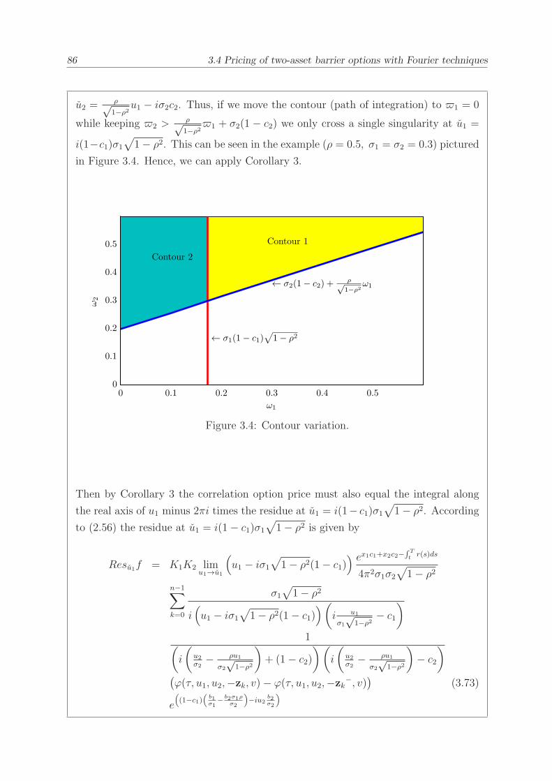
86 3.4 Pricing of two-asset barrier options with Fourier techniques
u2 =ρ√1−ρ2
u1 − iσ2c2. Thus, if we move the contour (path of integration) to 1 = 0
while keeping 2 >ρ√1−ρ2
1 + σ2(1 − c2) we only cross a single singularity at u1 =
i(1−c1)σ1√
1− ρ2. This can be seen in the example (ρ = 0.5, σ1 = σ2 = 0.3) pictured
in Figure 3.4. Hence, we can apply Corollary 3.
ω2
ω1
Contour 2
Contour 1
← σ1(1− c1)√
1− ρ2
← σ2(1− c2) +ρ√1−ρ2
ω1
0 0.1 0.2 0.3 0.4 0.50
0.1
0.2
0.3
0.4
0.5
Figure 3.4: Contour variation.
Then by Corollary 3 the correlation option price must also equal the integral along
the real axis of u1 minus 2πi times the residue at u1 = i(1− c1)σ1√
1− ρ2. Accordingto (2.56) the residue at u1 = i(1− c1)σ1
√
1− ρ2 is given by
Resu1f = K1K2 limu1→u1
(
u1 − iσ1√
1− ρ2(1− c1)) ex1c1+x2c2−
∫ Tt
r(s)ds
4π2σ1σ2√
1− ρ2n−1∑
k=0
σ1√
1− ρ2
i(
u1 − iσ1√
1− ρ2(1− c1))(
i u1
σ1
√1−ρ2− c1
)
1(
i
(
u2
σ2− ρu1
σ2
√1−ρ2
)
+ (1− c2))(
i
(
u2
σ2− ρu1
σ2
√1−ρ2
)
− c2)
(ϕ(τ, u1, u2,−zk, v)− ϕ(τ, u1, u2,−zk−, v)
)(3.73)
e
(
(1−c1)(
b1σ1
− b2σ1ρσ2
)
−iu2b2σ2
)

3 Pricing of barrier options within stochastic covariance model 87
= K1K2ex1c1+x2c2−
∫ Tt
r(s)ds
4π2σ1σ2√
1− ρ2n−1∑
k=0
iσ1√
1− ρ2
1(
i
(
u2
σ2− ρu1
σ2
√1−ρ2
)
+ (1− c2))(
i
(
u2
σ2− ρu1
σ2
√1−ρ2
)
− c2)
(ϕ(τ, u1, u2,−zk, v)− ϕ(τ, u1, u2,−zk−, v)
)(3.74)
e
(
(1−c1)(
b1σ1
− b2σ1ρσ2
)
−iu2b2σ2
)
,
where f is the integrand in (3.72). Hence, the new pricing formula is indicated by
C2C (t, S1, S2, B1, B2, v) =n−1∑
k=0
(
− 2πi
∫ i2+∞
i2−∞Resu1du2
+ex1c1+x2c2−
∫ Tt
r(s)ds
4π2σ1σ2√
1− ρ2∫ i2+∞
i2−∞
∫ ∞
−∞hC(u)
(ϕ(τ,u,−zk, v)− ϕ(τ,u,−zk−, v)
)(3.75)
e(iu1(− b1
σ1
√1−ρ2
+b2ρ
σ2
√1−ρ2
)−iu2b2σ2
)du1du2
)
,
1 = 0, 2 > σ2(1− c2).
In a next step we want to move 2 to 0. This time we pass singularities at u2 =ρu1√1−ρ2
+ iσ2(1− c2). The residue for the second integral in (3.75) is given by
Res(2)u2f2 = K1K2 lim
u2→u2
(u2 −ρu1
√
1− ρ2− iσ2(1− c2))
ex1c1+x2c2−∫ Tt
r(s)ds
4π2σ1σ2√
1− ρ2n−1∑
k=0
1
(i u1
σ1
√1−ρ2
+ (1− c1))(i u1
σ1
√1−ρ2− c1)
σ2
i
(
u2 − ρu1√1−ρ2− iσ2(1− c2)
)(
i
(
u2
σ2− ρu1
σ2
√1−ρ2
)
− c2)
(ϕ(τ, u1, u2,−zk, v)− ϕ(τ, u1, u2,−zk−, v)
)(3.76)
e
(
iu1
(
− b1
σ1
√1−ρ2
+b2ρ
σ2
√1−ρ2
)
−iu2b2σ2
)

88 3.4 Pricing of two-asset barrier options with Fourier techniques
= K1K2ex1c1+x2c2−
∫ Tt
r(s)ds
4π2σ1σ2√
1− ρ2n−1∑
k=0
iσ2
1(
i u1
σ1
√1−ρ2
+ (1− c1))(
i u1
σ1
√1−ρ2− c1
)
(ϕ(τ, u1, u2,−zk, v)− ϕ(τ, u1, u2,−zk−, v)
)(3.77)
e
(
iu1
(
− b1
σ1
√1−ρ2
+b2ρ
σ2
√1−ρ2
)
−iu2b2σ2
)
,
where f2 is the integrand of the second integral in (3.75). The residue for the first
integral is given by
Res(1)u2f1 = −2πiK1K2 lim
u2→u2
(u2 −ρu1
√
1− ρ2− iσ2(1− c2))
ex1c1+x2c2−∫ Tt
r(s)ds
4π2σ1σ2√
1− ρ2n−1∑
k=0
iσ1√
1− ρ2
σ2
i
(
u2 − ρu1√1−ρ2− iσ2(1− c2)
)(
i
(
u2
σ2− ρu1
σ2
√1−ρ2
)
− c2)
(ϕ(τ, u1, u2,−zk, v)− ϕ(τ, u1, u2,−zk−, v)
)
e
(
iu1
(
− b1
σ1
√1−ρ2
+b2ρ
σ2
√1−ρ2
)
−iu2b2σ2
)
= K1K2ex1c1+x2c2−
∫ Tt
r(s)ds
2πσ2n−1∑
k=0
iσ2(ϕ(τ, u1, u2,−zk, v)− ϕ(τ, u1, u2,−zk−, v)
)
e
(
(1−c1)(
b1σ1
− b2σ1ρσ2
)
−iu2b2σ2
)
, (3.78)
where f1 is the integrand of the first integral in (3.75). Thus, the pricing formula with
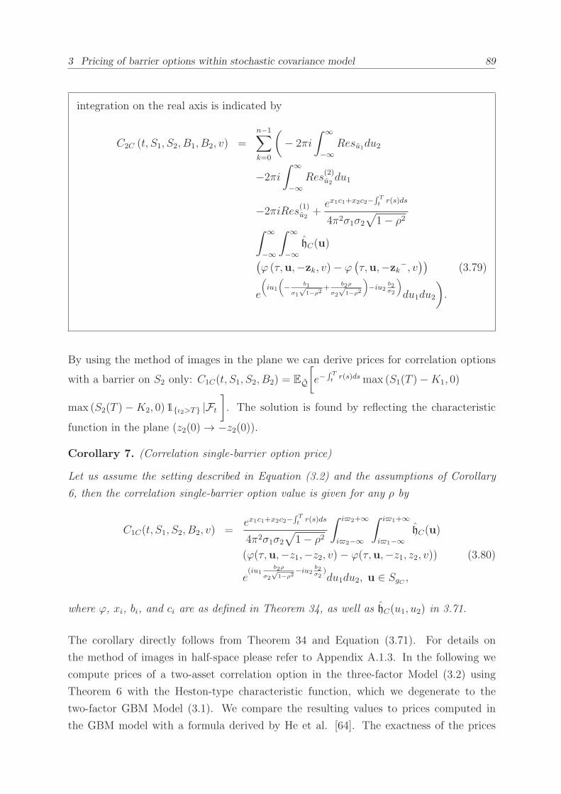
3 Pricing of barrier options within stochastic covariance model 89
integration on the real axis is indicated by
C2C (t, S1, S2, B1, B2, v) =n−1∑
k=0
(
− 2πi
∫ ∞
−∞Resu1du2
−2πi∫ ∞
−∞Res
(2)u2du1
−2πiRes(1)u2+ex1c1+x2c2−
∫ Tt
r(s)ds
4π2σ1σ2√
1− ρ2∫ ∞
−∞
∫ ∞
−∞hC(u)
(ϕ (τ,u,−zk, v)− ϕ
(τ,u,−zk−, v
))(3.79)
e
(
iu1
(
− b1
σ1
√1−ρ2
+b2ρ
σ2
√1−ρ2
)
−iu2b2σ2
)
du1du2
)
.
By using the method of images in the plane we can derive prices for correlation options
with a barrier on S2 only: C1C(t, S1, S2, B2) = EQ
[
e−∫ Tt
r(s)ds max (S1(T )−K1, 0)
max (S2(T )−K2, 0)1ι2>T |Ft
]
. The solution is found by reflecting the characteristic
function in the plane (z2(0)→ −z2(0)).
Corollary 7. (Correlation single-barrier option price)
Let us assume the setting described in Equation (3.2) and the assumptions of Corollary
6, then the correlation single-barrier option value is given for any ρ by
C1C(t, S1, S2, B2, v) =ex1c1+x2c2−
∫ Tt
r(s)ds
4π2σ1σ2√
1− ρ2∫ i2+∞
i2−∞
∫ i1+∞
i1−∞hC(u)
(ϕ(τ,u,−z1,−z2, v)− ϕ(τ,u,−z1, z2, v)) (3.80)
e(iu1
b2ρ
σ2
√1−ρ2
−iu2b2σ2
)du1du2, u ∈ SgC ,
where ϕ, xi, bi, and ci are as defined in Theorem 34, as well as hC(u1, u2) in 3.71.
The corollary directly follows from Theorem 34 and Equation (3.71). For details on
the method of images in half-space please refer to Appendix A.1.3. In the following we
compute prices of a two-asset correlation option in the three-factor Model (3.2) using
Theorem 6 with the Heston-type characteristic function, which we degenerate to the
two-factor GBM Model (3.1). We compare the resulting values to prices computed in
the GBM model with a formula derived by He et al. [64]. The exactness of the prices
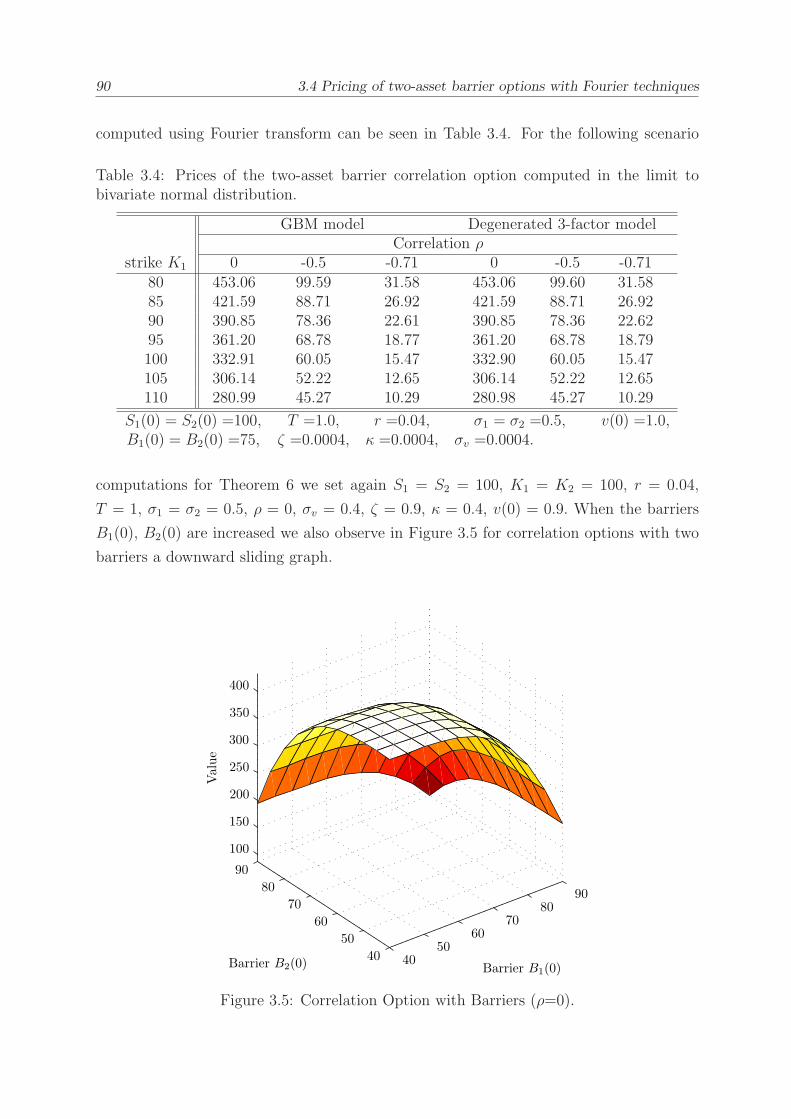
90 3.4 Pricing of two-asset barrier options with Fourier techniques
computed using Fourier transform can be seen in Table 3.4. For the following scenario
Table 3.4: Prices of the two-asset barrier correlation option computed in the limit tobivariate normal distribution.
GBM model Degenerated 3-factor modelCorrelation ρ
strike K1 0 -0.5 -0.71 0 -0.5 -0.7180 453.06 99.59 31.58 453.06 99.60 31.5885 421.59 88.71 26.92 421.59 88.71 26.9290 390.85 78.36 22.61 390.85 78.36 22.6295 361.20 68.78 18.77 361.20 68.78 18.79100 332.91 60.05 15.47 332.90 60.05 15.47105 306.14 52.22 12.65 306.14 52.22 12.65110 280.99 45.27 10.29 280.98 45.27 10.29
S1(0) = S2(0) =100, T =1.0, r =0.04, σ1 = σ2 =0.5, v(0) =1.0,B1(0) = B2(0) =75, ζ =0.0004, κ =0.0004, σv =0.0004.
computations for Theorem 6 we set again S1 = S2 = 100, K1 = K2 = 100, r = 0.04,
T = 1, σ1 = σ2 = 0.5, ρ = 0, σv = 0.4, ζ = 0.9, κ = 0.4, v(0) = 0.9. When the barriers
B1(0), B2(0) are increased we also observe in Figure 3.5 for correlation options with two
barriers a downward sliding graph.
Value
Barrier B2(0) Barrier B1(0)40
5060
7080
90
40
50
60
70
80
90
100
150
200
250
300
350
400
Figure 3.5: Correlation Option with Barriers (ρ=0).
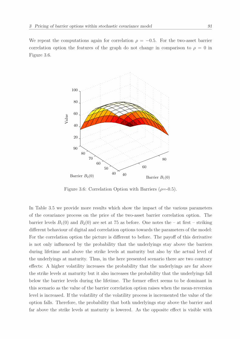
3 Pricing of barrier options within stochastic covariance model 91
We repeat the computations again for correlation ρ = −0.5. For the two-asset barrier
correlation option the features of the graph do not change in comparison to ρ = 0 in
Figure 3.6.
Value
Barrier B2(0) Barrier B1(0)40
60
80
4050
6070
8090
20
40
60
80
100
Figure 3.6: Correlation Option with Barriers (ρ=-0.5).
In Table 3.5 we provide more results which show the impact of the various parameters
of the covariance process on the price of the two-asset barrier correlation option. The
barrier levels B1(0) and B2(0) are set at 75 as before. One notes the – at first – striking
different behaviour of digital and correlation options towards the parameters of the model:
For the correlation option the picture is different to before. The payoff of this derivative
is not only influenced by the probability that the underlyings stay above the barriers
during lifetime and above the strike levels at maturity but also by the actual level of
the underlyings at maturity. Thus, in the here presented scenario there are two contrary
effects: A higher volatility increases the probability that the underlyings are far above
the strike levels at maturity but it also increases the probability that the underlyings fall
below the barrier levels during the lifetime. The former effect seems to be dominant in
this scenario as the value of the barrier correlation option raises when the mean-reversion
level is increased. If the volatility of the volatility process is incremented the value of the
option falls. Therefore, the probability that both underlyings stay above the barrier and
far above the strike levels at maturity is lowered. As the opposite effect is visible with
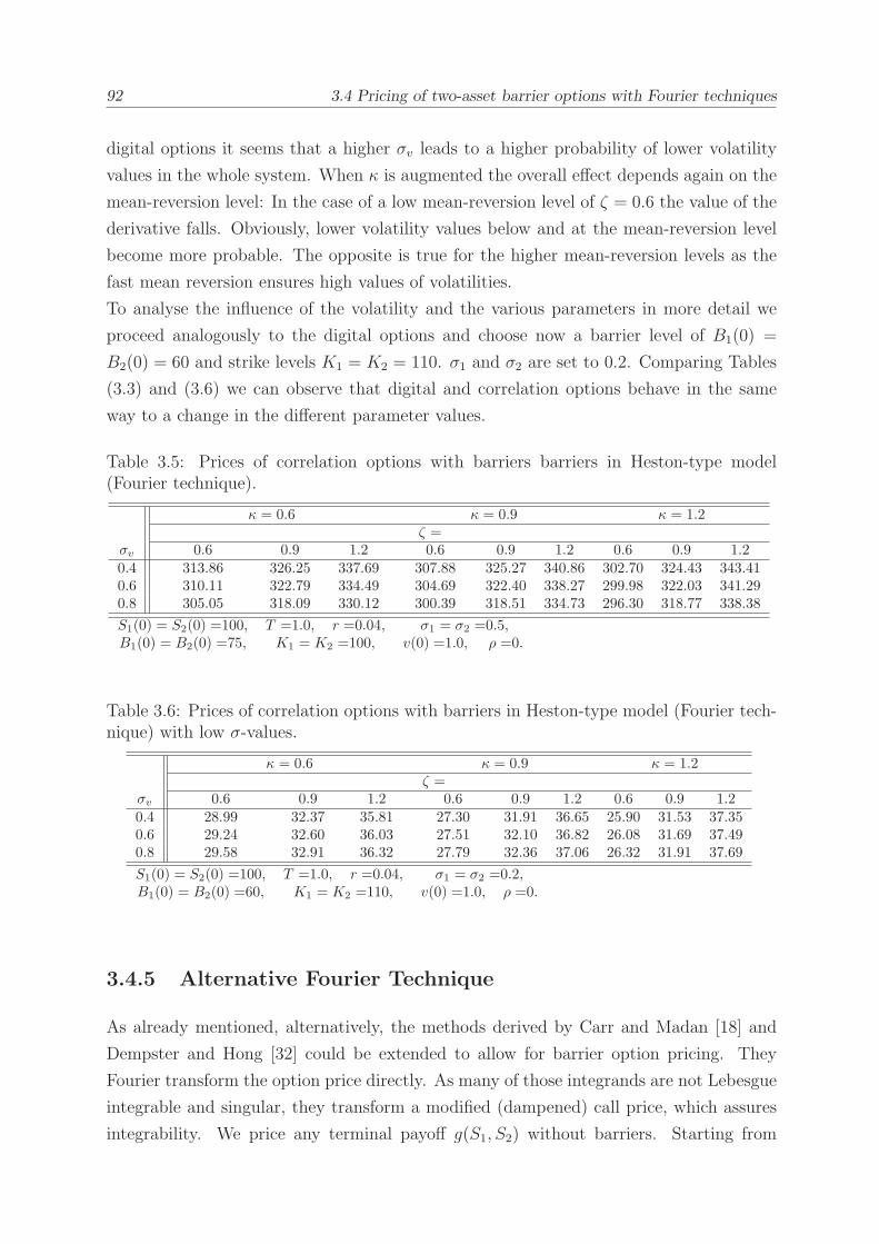
92 3.4 Pricing of two-asset barrier options with Fourier techniques
digital options it seems that a higher σv leads to a higher probability of lower volatility
values in the whole system. When κ is augmented the overall effect depends again on the
mean-reversion level: In the case of a low mean-reversion level of ζ = 0.6 the value of the
derivative falls. Obviously, lower volatility values below and at the mean-reversion level
become more probable. The opposite is true for the higher mean-reversion levels as the
fast mean reversion ensures high values of volatilities.
To analyse the influence of the volatility and the various parameters in more detail we
proceed analogously to the digital options and choose now a barrier level of B1(0) =
B2(0) = 60 and strike levels K1 = K2 = 110. σ1 and σ2 are set to 0.2. Comparing Tables
(3.3) and (3.6) we can observe that digital and correlation options behave in the same
way to a change in the different parameter values.
Table 3.5: Prices of correlation options with barriers barriers in Heston-type model(Fourier technique).
κ = 0.6 κ = 0.9 κ = 1.2ζ =
σv 0.6 0.9 1.2 0.6 0.9 1.2 0.6 0.9 1.20.4 313.86 326.25 337.69 307.88 325.27 340.86 302.70 324.43 343.410.6 310.11 322.79 334.49 304.69 322.40 338.27 299.98 322.03 341.290.8 305.05 318.09 330.12 300.39 318.51 334.73 296.30 318.77 338.38
S1(0) = S2(0) =100, T =1.0, r =0.04, σ1 = σ2 =0.5,B1(0) = B2(0) =75, K1 = K2 =100, v(0) =1.0, ρ =0.
Table 3.6: Prices of correlation options with barriers in Heston-type model (Fourier tech-nique) with low σ-values.
κ = 0.6 κ = 0.9 κ = 1.2ζ =
σv 0.6 0.9 1.2 0.6 0.9 1.2 0.6 0.9 1.20.4 28.99 32.37 35.81 27.30 31.91 36.65 25.90 31.53 37.350.6 29.24 32.60 36.03 27.51 32.10 36.82 26.08 31.69 37.490.8 29.58 32.91 36.32 27.79 32.36 37.06 26.32 31.91 37.69
S1(0) = S2(0) =100, T =1.0, r =0.04, σ1 = σ2 =0.2,B1(0) = B2(0) =60, K1 = K2 =110, v(0) =1.0, ρ =0.
3.4.5 Alternative Fourier Technique
As already mentioned, alternatively, the methods derived by Carr and Madan [18] and
Dempster and Hong [32] could be extended to allow for barrier option pricing. They
Fourier transform the option price directly. As many of those integrands are not Lebesgue
integrable and singular, they transform a modified (dampened) call price, which assures
integrability. We price any terminal payoff g(S1, S2) without barriers. Starting from
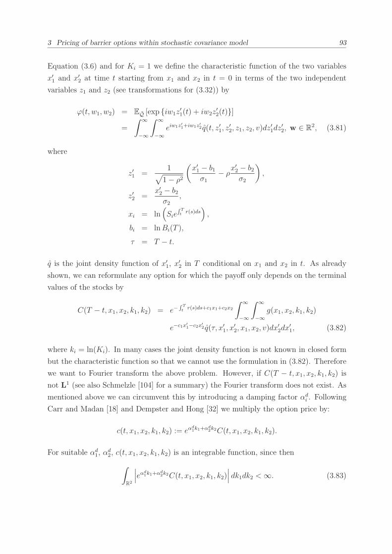
3 Pricing of barrier options within stochastic covariance model 93
Equation (3.6) and for Ki = 1 we define the characteristic function of the two variables
x′1 and x′2 at time t starting from x1 and x2 in t = 0 in terms of the two independent
variables z1 and z2 (see transformations for (3.32)) by
ϕ(t, w1, w2) = EQ [exp iw1z′1(t) + iw2z
′2(t)]
=
∫ ∞
−∞
∫ ∞
−∞eiw1z
′1+iw1z
′2 q(t, z′1, z
′2, z1, z2, v)dz
′1dz
′2, w ∈ R
2, (3.81)
where
z′1 =1
√
1− ρ2
(x′1 − b1σ1
− ρx′2 − b2σ2
)
,
z′2 =x′2 − b2σ2
,
xi = ln(
Sie∫ Tt
r(s)ds)
,
bi = lnBi(T ),
τ = T − t.
q is the joint density function of x′1, x′2 in T conditional on x1 and x2 in t. As already
shown, we can reformulate any option for which the payoff only depends on the terminal
values of the stocks by
C(T − t, x1, x2, k1, k2) = e−∫ Tt
r(s)ds+c1x1+c2x2
∫ ∞
−∞
∫ ∞
−∞g(x1, x2, k1, k2)
e−c1x′1−c2x
′2 q(τ, x′1, x
′2, x1, x2, v)dx
′2dx
′1, (3.82)
where ki = ln(Ki). In many cases the joint density function is not known in closed form
but the characteristic function so that we cannot use the formulation in (3.82). Therefore
we want to Fourier transform the above problem. However, if C(T − t, x1, x2, k1, k2) is
not L1 (see also Schmelzle [104] for a summary) the Fourier transform does not exist. As
mentioned above we can circumvent this by introducing a damping factor αdi . Following
Carr and Madan [18] and Dempster and Hong [32] we multiply the option price by:
c(t, x1, x2, k1, k2) := eαd1k1+αd
2k2C(t, x1, x2, k1, k2).
For suitable αd1, α
d2, c(t, x1, x2, k1, k2) is an integrable function, since then
∫
R2
∣∣∣eα
d1k1+αd
2k2C(t, x1, x2, k1, k2)∣∣∣ dk1dk2 <∞. (3.83)

94 3.4 Pricing of two-asset barrier options with Fourier techniques
Along the lines of Dempster and Hong [32] we derive the Fourier transform of the modified
double-digital option price (without barriers), i.e. g(x1, x2) = 1x1>k1,x2>k2, where ki =
lnKi.
cD(w1, w2) =
∫ ∞
−∞
∫ ∞
−∞eiw1k1+iw2k2cD(t, x1, x2, k1, k2)dk2dk1
=
∫ ∞
−∞
∫ ∞
−∞e(α
d1+iw1)k1+(αd
2+iw2)k2e−∫ Tt
r(s)ds+c1x1+c2x2
∫ ∞
k1
∫ ∞
k2
e−c1x′1−c2x
′2 q(τ, x′1, x
′2, x1, x2, v)dx
′2dx
′1dk2dk1
=
∫ ∞
−∞
∫ ∞
−∞e−
∫ Tt
r(s)ds+c1x1+c2x2 q(τ, x′1, x′2, x1, x2, v)
∫ x′1
−∞
∫ x′2
−∞e(α
d1+iw1)k1+(αd
2+iw2)k2e−c1x′1−c2x
′2dk2dk1dx
′2dx
′1
= e−∫ Tt
r(s)ds+c1x1+c2x2
∫ ∞
−∞
∫ ∞
−∞
e(αd1−c1+iw1)x′
1+(αd2−c2+iw2)x′
2 q(τ, x′1, x′2, x1, x2, v)
(αd1 + iw1)(αd
2 + iw2)dx′2dx
′1
= e−∫ Tt
r(s)ds+c1x1+c2x2
∫ ∞
−∞
∫ ∞
−∞
e(αd1−c1+iw1)
(√1−ρ2σ1z
′1+b1+ρσ1z
′2
)
(αd1 + iw1)(αd
2 + iw2)
e(αd2−c2+iw2)(z′2σ2+b2)q(τ, z′1, z
′2, z1, z2, v)dz
′2dz
′1
= e−∫ Tt
r(s)ds+c1x1+c2x2e(α
d1−c1+iw1)b1+(αd
2−c2+iw2)b2
(αd1 + iw1)(αd
2 + iw2)ϕ(τ, u1, u2, v),
where
u1 = σ1√
1− ρ2(w1 − i
(αd1 − c1
)),
u2 = σ2(u2 − i
(αd2 − c2
))+ ρσ1
(w1 − i
(αd1 − c1
)).
We can apply the Theorem of Fubini in the forth line due to 3.83.
The damping factor improves the integrability on the negative real axis. A sufficient
condition for cD to be square-integrable is the finiteness of cD(0, 0), which can be achieved
by choosing αdi accordingly. Then the inversion of cD converges to cD in L2- norm in line
with Plancherel’s Theorem (see Theorem 11). Comparing u1 to (3.67) and the there
defined strip of regularity for u1 we can observe that the introduction of the damping
factor αdi ensures in a similar manner as the application of the generalized Fourier inversion
(integration in the complex plane) integrability.

3 Pricing of barrier options within stochastic covariance model 95
The price of a digital option without barriers is given by
CD(τ, S1, S2, K1, K2, v) =e−α1k1−α2k2
4π2∫ ∞
−∞
∫ ∞
−∞e−i(w1k1+w2k2)cD(τ, w1, w2)dw2dw1. (3.84)
The value of the barrier option in the three-factor model can be found when we apply
the method of images in a wedge (see He et al. [64], Carslaw and Jaeger [19], p. 277f,
Sommerfeld [109]) to the characteristic function in accordance with the proof of Theorem
34.
Corollary 8. (Double-digital barrier option price with alternative method)
Let us assume
i. the setting described in Equation (3.2),
ii. the existence of an affine characteristic function,
iii. ρ = − cos(πn
), where n is a natural number and n > 1, and that
iv. there are αd1, α
d2 so that exp α1x1 + α2x2CD ∈ L2.
Then the price of a two-asset digital barrier option (see (3.66) for the payoff profile) is:
C2D(t, S1, S2, K1, K2, B1, B2, v) =e−α1k1−α2k2
4π2
∫ ∞
−∞
∫ ∞
−∞e−i(w1k1+w2k2)
c2D(w1, w2)dw2dw1, (3.85)
where
c2D(w) =e−
∫ Tt
r(s)ds+c1x1+c2x2e(αd1−c1+iw1)b1+(αd
2−c2+iw2)b2
(αd1 + iw1)(αd
2 + iw2)n−1∑
k=0
(ϕ (τ,u,−zk, v)− ϕ
(τ,u,−z−k , v
)),
where ϕ, z(−)k1 and z
(−)k2 are given Theorem 34. The convergence is in L2-norm.
Similarly, the price of the correlation barrier option can be derived. The transform of the

96 3.4 Pricing of two-asset barrier options with Fourier techniques
dampened correlation option price is given by
cC(w1, w2) =
∫ ∞
−∞
∫ ∞
−∞e(iw1+αd
1)k1+(iw2+αd2)k2e−
∫ Tt
r(s)ds+c1x1+c2x2
∫ ∞
k1
∫ ∞
k2
e−c1x′1−c2x
′2
(
ex′1 − ek1
)(
ex′2 − ek2
)
q(τ, x′1, x′2, x1, x2, v)dx
′2dx
′1dk2dk1
=
∫ ∞
−∞
∫ ∞
−∞e−
∫ Tt
r(s)ds+c1x1+c2x2 q(τ, x′1, x′2, x1, x2, v)
∫ x′1
−∞
∫ x′2
−∞e(iw1+αd
1)k1
e(iw2+αd2)k2e−c1x
′1−c2x
′2
(
ex′1 − ek1
)(
ex′2 − ek2
)
dk2dk1dx′2dx
′1
= e−∫ Tt
r(s)ds+c1x1+c2x2
∫ ∞
−∞
∫ ∞
−∞qT (x
′1, x
′2, v)
ex′1(α
d1+1−c1+iw1)(αd
1 + 1 + iw1)− ex′1(α
d1+1−c1+iw1)(αd
1 + iw1)
(αd1 + iw1)(αd
1 + 1 + iw1)
ex′2(α
d2+iw2+1−c2)(αd
2 + 1 + iw2)− ex′2(α
d2+iw2+1−c2)(αd
2 + iw2)
(αd2 + iw2 + 1)(αd
2 + iw2)dx′2dx
′1
= e−∫ Tt
r(s)ds+c1x1+c2x2
∫ ∞
−∞
∫ ∞
−∞
ex′1(α
d1+1−c1+iw1)
(αd1 + iw1)(αd
1 + 1 + iw1)
ex′2(α
d2+iw2+1−c2)
(αd2 + iw2 + 1)(αd
2 + iw2)qT (x
′1, x
′2, v)dx
′2dx
′1
= e−∫ Tt
r(s)ds+c1x1+c2x2
∫ ∞
−∞
∫ ∞
−∞qT (z
′1, z
′2, v)
e(√
1−ρ2σ1z′1+b1+ρσ1z
′2)(α
d1+1−c1+iw1)e(z
′2σ2+b2)(αd
2+1−c2+iw2)
(αd1 + iu1)(αd
1 + 1 + iw1)(αd2 + 1 + iw2)(αd
2 + iw2)dz′2dz
′1
= e−∫ Tt
r(s)ds+c1x1+c2x2eb1(α
d1+1−c1+iw1)eb2(α
d2+1−c2+iw2)ϕ(τ, u′1, u
′2, v)
(αd1 + iw1)(αd
1 + 1 + iw1)(αd2 + iw2)(αd
2 + 1 + iw2),
where
u′1 = σ1√
1− ρ2(w1 − i
(αd1 + 1− c1
)),
u′2 = σ2(w2 − i
(αd2 + 1− c2
))+ ρσ1
(w1 −
(αd1 + 1− c1
)). (3.86)
Thus, the price of the correlation option is given by
CC(t, S1, S2, K1, K2, v) =e−α1k1−α2k2
4π2∫ ∞
−∞
∫ ∞
−∞e−i(w1k1+w2k2)cC(u1, u2)dw2dw1, (3.87)

3 Pricing of barrier options within stochastic covariance model 97
where
cC(w1, w2) =e−
∫ Tt
r(s)ds+c1x1+c2x2e(αd1+1−c1+iw1)b1+(αd
2+1−c2+iw2)b2(αd1 + iw1
) (αd1 + 1 + iw1
) (αd2 + iw2
) (αd2 + 1 + iw2
)ϕ (τ, u′1, u′2, v) ,
u′1 = σ1√
1− ρ2(w1 − i
(αd1 + 1− c1
)),
u′2 = σ2(w2 − i(αd2 + 1− c2)) + ρσ1
(w1 − i
(αd1 + 1− c1
)).
Corollary 9. (Correlation barrier option price with alternative method)
Let us assume
i. the setting described in Equation (3.2),
ii. the existence of an affine characteristic function,
iii. ρ = − cos(πn
), where n is a natural number and n > 1, and that
iv. there are αd1, α
d2 so that exp α1x1 + α2x2CD ∈ L2.
Then the price of a two-asset barrier correlation option (see (3.70) for the payoff profile)
is given by:
C2C(t, S1, S2, K1, K2, B1, B2, v) =e−α1k1−α2k2
4π2
∫ ∞
−∞
∫ ∞
−∞e−i(w1k1+w2k2)
c2C(u1, u2)dw2dw1, (3.88)
where
c2C(w1, w2) =e−
∫ Tt
r(s)ds+c1x1+c2x2e(αd1+1−c1+iw1)b1+(αd
2+1−c2+iw2)b2(αd1 + iw1
) (αd1 + 1 + iw1
) (αd2 + iw2
) (αd2 + 1 + iw2
)
n−1∑
k=0
(ϕ (τ,u,−zk+, v)− ϕ
(τ,u,−z−k , v
)),
u′1 = σ1√
1− ρ2(w1 − i
(αd1 + 1− c1
)),
u′2 = σ2(w2 − i(αd2 + 1− c2)) + ρσ1
(w1 − i
(αd1 + 1− c1
)),
where ϕ, z(−)k1 and z
(−)k2 are given Theorem 34. The convergence is in L2-norm.

98 3.5 Pricing of two-asset barrier options with PDE techniques
3.4.6 Random correlations
The restriction of the solution for the two-asset barrier options to correlations ρ =
− cos (πn) with n ∈ N might seem rather restrictive because all possible correlations are
negative for n > 2. We can, however, loosen this constraint. The assumption that the
correlation takes the attainable values ρn randomly with a probability pn makes positive
expected correlations achievable. For example, if we assume that p1 = p2 =12and pi = 0,
for i > 2 then the expected correlation is 12with variance 1
4.
Theorem 35. (Random correlation)
Let us assume that the correlation ρ can take any value ρn = − cos πnwith a positive
probability pn and that this probability pn is known. Then, the value of any derivative is
given as the weighted sum
C(t, S1, S2, v) =∞∑
i=1
pnC(ρ=−cosπn)(t, S1, S2, v). (3.89)
Remark 13. Given this assumption E(ρ) > 0 is attainable, although most of the possible
values for ρ are actually negative.
3.4.7 Conclusion
In this section we have shown how to derive easily attainable and quickly computable
solutions to a range of two-asset barrier options in a stochastic covariance framework
for a special correlation structure. This framework is extended to allow for a random
correlation structure. The formulas derived can be computed via fast Fourier transform
following the transformations done by Dempster and Hong [33] but even without the
adoption of the fast Fourier transform the formulas can be quickly evaluated.
3.5 Pricing of two-asset barrier options with PDE
techniques
In the following we use the method of separation and the solution to well-known ODEs
to find pricing techniques for valuing options for any ρ. In Subsection 3.5.1 we use our
knowledge about affine characteristic functions and the PDEs which they solve to find a
simple extension to the solution He et al. proposed for two correlated geometric Brownian
motions for our three-factor stochastic covariance Model (3.2). Moreover, we derive the
3 Pricing of barrier options within stochastic covariance model 99
survival probabilities.
3.5.1 General pricing formulas for two-asset barrier options ex-
ploiting the affine form in v
The System (3.6) can be solved for a group of models included in the general framework
(3.2), i.e. for specific values of the parameters γ and ν. This group is characterised by
the existence of an affine characteristic function. For these models a feasible and easily
manageable solution for the pricing of two-asset barrier options can be found:
Theorem 36. (Barrier option pricing in R2 with PDE technique)
Let us assume the setting described in Equation (3.2) and the existence of an affine char-
acteristic function. Then the price of a two-asset barrier option (see (3.4) for the payoff
profile) in the three-factor stochastic volatility model is given by
CB (t, S1, S2, B1, B2, v) =ex1c1+x2c2−
∫ Tt
r(s)ds
σ1σ2√
1− ρ2∫ ∞
−∞
∫ ∞
−∞g(x′1, x
′2)
e−x′1c1−x′
2c2q (τ, x1, x2, x′1, x
′2, v) dx
′1dx
′2, (3.90)
where
xi = lnSie
∫ Tt
r(s)ds
Ki
,
q (τ, x1, x2, x′1, x
′2, v) =
2
βp
∫ ∞
0
λV (τ, λ) (3.91)
∞∑
n=1
sin
(nπθ′pβp
)
sin
(nπθpβp
)
Jnπβp
(λrp) Jnπβp
(λr′p)dλ,
tan βp = −√
1− ρ2ρ
, β ∈ [0, π] ,
rp =
√
1
(1− ρ2)
(x1 − b1σ1
− ρx2 − b2σ2
)2
+
(x2 − b2σ2
)2
,
tan(θp) =x2−b2σ2
1√1−ρ2
(x1−b1σ1− ρx2−b2
σ2
) , θp ∈ [0, βp] ,
c1 =σ1 − σ2ρ
2σ1(1− ρ2), c2 =
σ2 − σ1ρ2σ2(1− ρ2)
,
100 3.5 Pricing of two-asset barrier options with PDE techniques
where V (τ, λ) solves the PDE given in (3.100) and Jς(x) denotes the Bessel function of
the first kind.
Proof.
We start from (3.32) and separate q(τ, z1, z2, v) = H(z1, z2)V (τ, v). We get
∂V
∂τH =
1
2v2νV
∂2H
∂z21+
1
2v2νV
∂2H
∂z22− v2ν σ
21 + σ2
2 − 2ρσ1σ28(1− ρ2) HV
+1
2σ2vv
2γ ∂2V
∂v2H + κ(ζ − v)∂V
∂vH. (3.92)
Dividing by H we obtain
∂V
∂τ=
1
2v2ν
V
H
(∂2H
∂z21+∂2H
∂z22
)
− v2ν σ21 + σ2
2 − 2ρσ1σ28(1− ρ2) V
+1
2σ2vv
2γ ∂2V
∂v2+ κ(ζ − v)∂V
∂v. (3.93)
Furthermore, we set1
2
(∂2H
∂z21+∂2H
∂z22
)
= −λ2
2H. (3.94)
By transforming z1 and z2 in Equation (3.94) to polar coordinates the vertical
boundary is described by the angle tan θp = −√
1−ρ2
ρand the horizontal bound-
ary by θp = 0. Thus, the bounded area for which the PDE is defined is a
wedge Y = (rp cos (θp) , rp sin (θp)) : rp > 0, 0 < θp < βp ⊂ R2, where tan βp =
−√
1−ρ2
ρ, βp ∈ [0, π]. The boundary of the wedge is described by ∂Y =
(rp cos (θp) , rp sin (θp)) : rp ≥ 0, θp ∈ 0, βp ⊂ R2. Choosing a separable solution of
the form R(rp)Θ(θp) we get the following relationship
r2p
d2Rdr2p
R+ rp
dRdrp
R+ λ2r2p
+
d2Θdθ2p
Θ
= 0. (3.95)
We defined2Θ
dθ2p
Θ= −k2 and find
Θ(θp) ∼ A sin (kθp) + B cos (kθp) . (3.96)
Θ has to fulfil the boundary conditions Θ(0) = Θ(βp) = 0. Thus, B = 0 as k is real.
Hence,
kn =nπ
βp, n = 1, 2 . . . (3.97)

3 Pricing of barrier options within stochastic covariance model 101
The radial part is given by
(λrp)2 d2R
d (λrp)2 + (λrp)
dR
d (λrp)+((λrp)
2 − kn2)R = 0. (3.98)
As R(0) has to be well-behaved, the general solution of the radial part is
R(rp) ∼ Jkn (λrp) , (3.99)
where Jς(x) is the Bessel function of the first kind. We insert (3.94) in (3.93) and get
∂V
∂τ= −1
2v2νλ2V − v2ν σ
21 + σ2
2 − 2ρσ1σ28(1− ρ2) V
+1
2σ2vv
2γ ∂2V
∂v2+ κ(ζ − v)∂V
∂v, (3.100)
V (0, v) = 1. (3.101)
If the process possesses an affine-type characteristic function, (3.100) collapses to a system
of ODEs and the solution can be given by
q(τ, rp, θp, r
′p, θ
′p, v)
=
∫ ∞
0
V (τ, λ)∞∑
n=1
cn(λ)
sin
(nπθpβp
)
Jnπβp
(λrp) dλ. (3.102)
To determine cn(λ) we use the initial condition q (0, rp, θp, v) =1r′pδ(rp − r′p
)δ(θp − θ′p
).
Multiply (3.102) at τ = 0 by sin(
mπθpβp
)
and integrate over θp.
1
r′pδ(rp − r′p
)sin
(mπθ′pβp
)
=βp2
∫ ∞
0
cm(λ)Jmπβp
(λrp) dλ, (3.103)
where we use the integral identity∫ π
0sin (mx) sin (nx) dx = π
2δ(m− n) (see Arfken [7], p.
632) and, thus,∫ βp
0sin(
mπθpβp
)
sin(
nπθpβp
)
dθ = βp
2δ(m− n).
Finally, multiplying by rpJmπβp
(λ′rp) and integrating over rp results in the following solution
for cn(λ)
cm(λ′) =
2λ′
βpsin
(mπθ′pβp
)
Jmπβp
(λ′r′p
), (3.104)
where we use the Bessel function closure equation∫∞0xJς(ax)Jς(bx)dx = 1
aδ(a − b) (see

102 3.5 Pricing of two-asset barrier options with PDE techniques
Arfken [7], p. 648). Thus,
q(τ, rp, θp, r′p, θ
′p, v) =
2
βp
∫ ∞
0
λV (τ, λ)
∞∑
n=1
sin
(nπθ′pβp
)
sin
(nπθpβp
)
Jnπβp
(λrp) Jnπβp
(λr′p)dλ.
and,
p(x1(τ) ∈ dx1, x2(τ) ∈ dx2, x1(τ) > b1, x2(τ) > b2, v) =
=ec1x1+c2x2−
∫ Tt
r(s)ds
σ1σ2√
1− ρ2q (τ, x1, x2, x
′1, x
′2, v) dx
′1dx
′2, (3.105)
where xi denotes the minimum value xi takes in τ and1
σ1σ2
√1−ρ2
is the Jacobi determinant.
Remark 14. If the three-factor model degenerates to a two-factor GBM model then (3.91)
is consistent with the formula He et al. [64] found.
qGBM (τ, x1, x2, x′1, x
′2, v) =
2
βpτe−σ2
1+σ22−2ρσ1σ2
8(1−ρ2)τ
∞∑
n=1
e−r2p+r′p
2
2τ
sin
(nπθ′pβp
)
sin
(nπθpβp
)
Inπβp
(r′prp
τ
)
, (3.106)
where Iς(x) denotes the modified Bessel function of the first kind.
Proof.
If the three-factor model degenerates to a two-factor GBM model then (3.91) is consistent
with the formula He et al. [64] found:
qGBM(τ, x1, x2, v) =2
βp
∫ ∞
0
λe− 1
2(λ2τ+
σ21+σ2
2−2ρσ1σ24(1−ρ2)
τ)
∞∑
n=1
sin
(nπθ′pβp
)
sin
(nπθpβp
)
Jnπβp
(λrp) Jnπβp
(λr′p)dλ
=2
βpτe−σ2
1+σ22−2ρσ1σ2
8(1−ρ2)τ
∞∑
n=1
e−r2p+r′p
2
2τ sin
(nπθ′pβp
)
sin
(nπθpβp
)
Inπβp
(r′prp
τ
)
, (3.107)

3 Pricing of barrier options within stochastic covariance model 103
where we used the formula (see Gradshtein [59], 6.633)
∫ ∞
0
xe−c2xJς(ax)Jς(bx)dx =1
2c2e−
(a2+b2)
4c2 Iς
(ab
2c2
)
, (3.108)
with Iς(
ab2c2
), the modified Bessel function of the first kind.
One of the models for which the affine characteristic function exists is the model with
the Heston-type third factor. The price of a two-asset barrier option is presented in the
following corollary.
Corollary 10. (Barrier option pricing in Heston-type model in R2 with PDE technique)
Let us assume the setting described in Equations (3.2) and (3.3) with ν = γ = 12. Then
the price of a two-asset barrier option (see (3.4) for the payoff profile) in the three-factor
stochastic volatility model is
CB (t, S1, S2, B1, B2, v) =ex1c1+x2c2−
∫ Tt
r(s)ds
σ1σ2√
1− ρ2∫ ∞
−∞
∫ ∞
−∞g(x′1, x
′2)
e−x′1c1−x′
2c2q (τ, x1, x2, x′1, x
′2, v) dx
′1dx
′2, (3.109)
where
xi = ln
(
Sie∫ Tt
r(s)ds
Ki
)
,
q (τ, x1, x2, x′1, x
′2, v) =
2
βp
∫ ∞
0
λe1
σ2v(AH(τ,λ)+BH(τ,λ)v)
(3.110)
∞∑
n=1
sin
(nπθ′pβp
)
sin
(nπθpβp
)
Jnπβp
(λrp) Jnπβp
(λr′p)dλ,
tan βp = −√
1− ρ2ρ
, β ∈ [0, π] ,
rp =
√
1
(1− ρ2)
(x1 − b1σ1
− ρx2 − b2σ2
)2
+
(x2 − b2σ2
)2
,
tan(θp) =x2−b2σ2
1√1−ρ2
(x1−b1σ1− ρx2−b2
σ2
) , θp ∈ [0, βp],
d = d(λ) =
√
κ2 + σ2v
(
λ2 +σ21 + σ2
2 − 2ρσ1σ24(1− ρ2)
)
,
c1 =σ1 − σ2ρ
2σ1(1− ρ2), c2 =
σ2 − σ1ρ2σ2(1− ρ2)
,
where AH and BH are given in (3.49) and (3.48).

104 3.5 Pricing of two-asset barrier options with PDE techniques
Proof.
Inserting (A.24) in (3.100) we find the same ODEs as before in (A.1.2). The solutions
follow.
We have seen before that the Ornstein-Uhlenbeck process also possesses a characteristic
function. The pricing formula for the two-asset barrier option can, thus, be indicated in
the same way as for the Heston-type model:
Corollary 11. (Barrier option pricing in a Stein and Stein-type model in R2 with PDE
technique)
Let us assume the setting described in Equation (3.2) with ν = 1 and γ = 0. Then the
price of a two-asset barrier option (see (3.4) for the payoff profile) in the three-factor
stochastic volatility model is given by
CB (t, S1, S2, B1, B2, v) =ex1c1+x2c2−
∫ Tt
r(s)ds
σ1σ2√
1− ρ2∫ ∞
−∞
∫ ∞
−∞g(x′1, x
′2)
e−x′1c1−x′
2c2q (τ, x1, x2, x′1, x
′2, v) dx
′1dx
′2, (3.111)
where
xi = ln
(
Sie∫ Tt
r(s)ds
Ki
)
,
q (τ, x1, x2, x′1, x
′2, v) =
2
βp
∫ ∞
0
λe1
σ2v(AS2(τ,λ)+BS2(τ,λ)v+CS2(τ,λ)v
2)(3.112)
∞∑
n=1
sin
(nπθ′pβp
)
sin
(nπθpβp
)
Jnπβp
(λrp) Jnπβp
(λr′p)dλ,
tan βp = −√
1− ρ2ρ
, β ∈ [0, π] ,
rp =
√
1
(1− ρ2)
(x1 − b1σ1
− ρx2 − b2σ2
)2
+
(x2 − b2σ2
)2
,
tan(θp) =x2−b2σ2
1√1−ρ2
(x1−b1σ1− ρx2−b2
σ2
) , θp ∈ [0, β],
where AS2, BS2 and CS2 are given in (3.59-3.61).
Proof.
Inserting (A.37) in (3.100) we find the same ODEs as before in (A.1.2). The solutions
follow.
3 Pricing of barrier options within stochastic covariance model 105
Using the Result (3.91) we can derive some more densities along the lines of Iyengar
[71], i.e. the density of the first hitting time ι′ and xi(ι′) and the survival probability, i.e.
px(ι′ ∈ dt′,x(ι′) ∈ ∂D) and px(ι′ < t′) with 0 ≤ t ≤ t′ ≤ T .
By using the same arguments as Daniels [28], Iyengar [71] and Metzler [88] we derive the
probability density px (ι′ ∈ dt′,x(ι′) ∈ ∂D) of the hitting time ι′, where ι′ = min (ι1, ι2),
and the density of x(ι′) = (x1(ι′), x2(ι
′)) in ι′. ∂D describes the boundaries with
(b1, x2(ι′))⋃
(x1(ι′), b2) ⊂ ∂D.
Theorem 37. (px (ι′ ∈ dt′,x(ι′) ∈ ∂D))
The probability density function px(ι′ ∈ dt′,x(ι′) ∈ ∂D) is given by
px (ι′ ∈ dt′,x(ι′) ∈ ∂D) = ec1x1+c2x2−∫ t′
tr(s)ds π
β2prp
∫ ∞
0
λV (t′, λ)
∞∑
n=1
nδn sin
(nπθpβp
)
Jnπβp
(λrp) Jnπβp
(λr′p)dλ∂Ddt′, (3.113)
where δn = (−1)n+1 if θ′p = βp and δn = 1 if θ′p = 0,
xi = ln
(
Sie∫ Tt
r(s)ds
Ki
)
,
rp =
√
1
(1− ρ2)
(x1 − b1σ1
− ρx2 − b2σ2
)2
+
(x2 − b2σ2
)2
,
tan (θp) =x2−b2σ2
1√1−ρ2
(x1−b1σ1− ρx2−b2
σ2
) .
Proof.
Using a similar argument to Daniels [28], Iyengar [71] and Metzler [88] and transforming
to polar coordinates it can be shown that
pz (ι′ ∈ dt′, z(ι′) ∈ ∂Y ) = ec1x1+c2x2−∫ t′
tr(s)ds
qz (ι′ ∈ dt′, z(ι′) ∈ ∂Y ) dz1dz2
=ec1x1+c2x2−
∫ t′
tr(s)ds
2[∂
∂nq(t, rp, θp, t
′, r′p, θ′p
)r′p
∣∣∣z∈∂Y
]
dr′pdθ′p,
where (b1, x2(ι′))⋃(x1(ι
′), b2) ⊂ ∂D, ∂Y describes ∂D in polar coordinates. ∂∂n
de-
notes the normal derivative, i.e. a directional derivative taken in the inward nor-

106 3.5 Pricing of two-asset barrier options with PDE techniques
mal (orthogonal) direction, to the boundary ∂Y in point z (z ∈ ∂Y ). x =(
σ1
(√
1− ρ2z1 + ρz2
)
+ b1, σ2z2 + b2
)
and (z1, z2) = rp(cos(θ′p), sin
(θ′p)). In our
case the (unit) normal vector n on the boundary is either (0, 1) for z = (rp, 0), i.e.
z2 = 0, or (sin (βp) ,− cos (βp)) for z = rp (cos (βp) , sin (βp)), i.e. z2 = −√
1−ρ2
ρz1. With
∂q
∂n= ∇q · n =
(∂q
∂r′p, ∂q
r′p∂θ′p
)
· (0, 1) = 1r′p
∂q
∂θ′pwe obtain for z = (rp, 0)
qz (ι′ ∈ dt′, z(ι′) ∈ ∂Y ) =
[1
2r′p
∂
∂θ′p
2r′pβp
∫ ∞
0
λV (t′, λ)
∞∑
n=1
sin
(nπθ′pβp
)
sin
(nπθpβp
)
Jnπβp
(λrp) Jnπβp
(λr′p)dλdr′pdθ
′p
]
θ′p=0,r′p≥0
=
[1
βp
∫ ∞
0
λV (t′, λ)
∞∑
n=1
nπ
βpcos
(nπθ′pβp
)
sin
(nπθpβp
)
Jnπβp
(λrp) Jnπβp
(λr′p)dλdr′pdθ
′p
]
θ′p=0,r′p≥0
=π
β2p
∫ ∞
0
λV (t′, λ)
∞∑
n=1
n sin
(nπθpβp
)
Jnπβp
(λrp) Jnπβp
(λr′p)dλdr′pdθ
′p
=π
r′pβ2p
∫ ∞
0
λV (t′, λ)∞∑
n=1
n sin
(nπθpβp
)
Jnπβp
(λrp) Jnπβp
(λr′p)dλdz′1dz
′2. (3.114)
The respective probability for z = rp(cos(βp), sin(βp)) can be derived by reflecting z about
the line z2 = tan(
βp
2
)
z1, i.e. the reflected θp = βp − θp.

3 Pricing of barrier options within stochastic covariance model 107
We insert the reflection in (3.114) and compute
qz (ι′ ∈ dt′, z(ι′) ∈ ∂Y ) =π
r′pβ2p
∫ ∞
0
λV (t′, λ)∞∑
n=1
n sin
(
nπθpβp
)
Jnπβp
(λrp) Jnπβp
(λr′p)dλdz′1dz
′2
= − π
r′pβ2p
∫ ∞
0
λV (t′, λ)∞∑
n=1
n sin
(nπθpβp
)
cos (nπ) Jnπβp
(λrp) Jnπβp
(λr′p)dλdz′1dz
′2. (3.115)
The survival probability can be obtained by integrating (3.91) over the wedge (see Iyengar
[71] and Metzler [88]).
Theorem 38. (Survival probability)
The survival probability px(ι′ > t′) is given by the following expression in polar coordinates.
px(ι′ > t′) = ec1x1+c2x2−∫ t′
tr(s)ds
∑
n=1,3,5...
4
πnsin
(nπθpβp
)∫ ∞
0
V (t′, λ) Jnπβp
(λrp)
∫ ∞
0
r′pJnπβp
(λr′p)dr′pdλ, (3.116)
where
xi = ln
(
Sie∫ Tt
r(s)ds
Ki
)
,
rp =
√
1
(1− ρ2)
(x1 − b1σ1
− ρx2 − b2σ2
)2
+
(x2 − b2σ2
)2
,
tan(θp) =x2−b2σ2
1√1−ρ2
(x1−b1σ1− ρx2−b2
σ2
) , θp ∈ [0, βp].
Proof.
The probability that x1 and x2 do not hit the barrier during lifetime in 0 ≤ t ≤ t′ ≤ T
can be obtained by integrating (3.91) over the wedge. This is facilitated by converting to
108 3.5 Pricing of two-asset barrier options with PDE techniques
polar coordinates.
px(ι′ > t′) = ec1x1+c2x2−∫ t′
tr(s)ds
∫ βp
0
∫ ∞
0
q(t, rp, θp, r
′p, θ
′p, v)r′pdr
′pdθ
′p
= ec1x1+c2x2−∫ t′
tr(s)ds
∞∑
n=1
2
nπsin
(nπθpβp
)∫ βp
0
nπ
βpsin
(nπθ′pβp
)
dθ′p
∫ ∞
0
λV (t′, λ) Jnπβp
(λrp)
∫ ∞
0
r′pJnπβp
(λr′p)dr′pdλ
= ec1x1+c2x2−∫ t′
tr(s)ds
∑
n=1,3,5...
4
πnsin
(nπθpβp
)∫ ∞
0
λV (t′, λ) Jnπβp
(λrp)
∫ ∞
0
r′pJnπβp
(λr′p)dr′pdλ.
If the three-factor model is degenerated to the two-factor model the probability is given
by (see Metzler [88])
pxGBM(ι′ > t′) = ec1x1+c2x2−∫ t′
tr(s)ds
∑
n=1,3,5...
4
πnt′sin
(nπθpβp
)
e−σ2
1+σ22−2ρσ1σ2
8(1−ρ2)t′
∫ ∞
0
r′pe−(
r2p+r′p2)
2t′ Inπβp
(rpr
′p
t′
)
dr′p
= ec1x1+c2x2−∫ t′
tr(s)ds
∑
n=1,3,5...
4
πnt′sin
(nπθpβp
)
e−σ2
1+σ22−2ρσ1σ2
8(1−ρ2)t′
rp
∫ ∞
0
e−(r2p+r′p
2)
2t′1
2
(
Inπβp
−1
(rpr
′p
t′
)
+ Inπβp
+1
(rpr
′p
t′
))
dr′p
= ec1x1+c2x2−∫ t′
tr(s)ds 2rp√
2πt′e−σ2
1+σ22−2ρσ1σ2
8(1−ρ2)t′
e−r2p4t′
∑
n=1,3,5...
1
nsin
(nπθpβp
)(
I−12
(r2p4t′
)
+ I+12
(r2p4t′
))
,
where we used the identities 2I ′ς(x) = Iς−1(x) + Iς+1(x) (see Abramowitz and Stegun [1],
9.6.26) and∫∞0e−bt2Iς(at)dt =
12
√πbe
a2
8b I ς2( a
2
8b) (see Gradshtein [59], 6.618).
3.5.2 Pricing of two-asset double-digital barrier options with
PDE techniques
In the following we are going to derive formulas to price two-asset barrier double-digital
options with two time-dependent barriers.
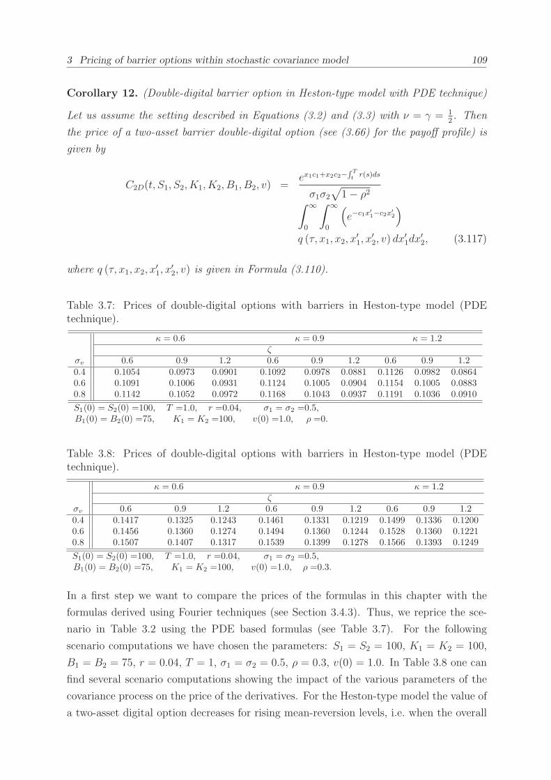
3 Pricing of barrier options within stochastic covariance model 109
Corollary 12. (Double-digital barrier option in Heston-type model with PDE technique)
Let us assume the setting described in Equations (3.2) and (3.3) with ν = γ = 12. Then
the price of a two-asset barrier double-digital option (see (3.66) for the payoff profile) is
given by
C2D(t, S1, S2, K1, K2, B1, B2, v) =ex1c1+x2c2−
∫ Tt
r(s)ds
σ1σ2√
1− ρ2∫ ∞
0
∫ ∞
0
(
e−c1x′1−c2x
′2
)
q (τ, x1, x2, x′1, x
′2, v) dx
′1dx
′2, (3.117)
where q (τ, x1, x2, x′1, x
′2, v) is given in Formula (3.110).
Table 3.7: Prices of double-digital options with barriers in Heston-type model (PDEtechnique).
κ = 0.6 κ = 0.9 κ = 1.2ζ
σv 0.6 0.9 1.2 0.6 0.9 1.2 0.6 0.9 1.20.4 0.1054 0.0973 0.0901 0.1092 0.0978 0.0881 0.1126 0.0982 0.08640.6 0.1091 0.1006 0.0931 0.1124 0.1005 0.0904 0.1154 0.1005 0.08830.8 0.1142 0.1052 0.0972 0.1168 0.1043 0.0937 0.1191 0.1036 0.0910
S1(0) = S2(0) =100, T =1.0, r =0.04, σ1 = σ2 =0.5,B1(0) = B2(0) =75, K1 = K2 =100, v(0) =1.0, ρ =0.
Table 3.8: Prices of double-digital options with barriers in Heston-type model (PDEtechnique).
κ = 0.6 κ = 0.9 κ = 1.2ζ
σv 0.6 0.9 1.2 0.6 0.9 1.2 0.6 0.9 1.20.4 0.1417 0.1325 0.1243 0.1461 0.1331 0.1219 0.1499 0.1336 0.12000.6 0.1456 0.1360 0.1274 0.1494 0.1360 0.1244 0.1528 0.1360 0.12210.8 0.1507 0.1407 0.1317 0.1539 0.1399 0.1278 0.1566 0.1393 0.1249
S1(0) = S2(0) =100, T =1.0, r =0.04, σ1 = σ2 =0.5,B1(0) = B2(0) =75, K1 = K2 =100, v(0) =1.0, ρ =0.3.
In a first step we want to compare the prices of the formulas in this chapter with the
formulas derived using Fourier techniques (see Section 3.4.3). Thus, we reprice the sce-
nario in Table 3.2 using the PDE based formulas (see Table 3.7). For the following
scenario computations we have chosen the parameters: S1 = S2 = 100, K1 = K2 = 100,
B1 = B2 = 75, r = 0.04, T = 1, σ1 = σ2 = 0.5, ρ = 0.3, v(0) = 1.0. In Table 3.8 one can
find several scenario computations showing the impact of the various parameters of the
covariance process on the price of the derivatives. For the Heston-type model the value of
a two-asset digital option decreases for rising mean-reversion levels, i.e. when the overall
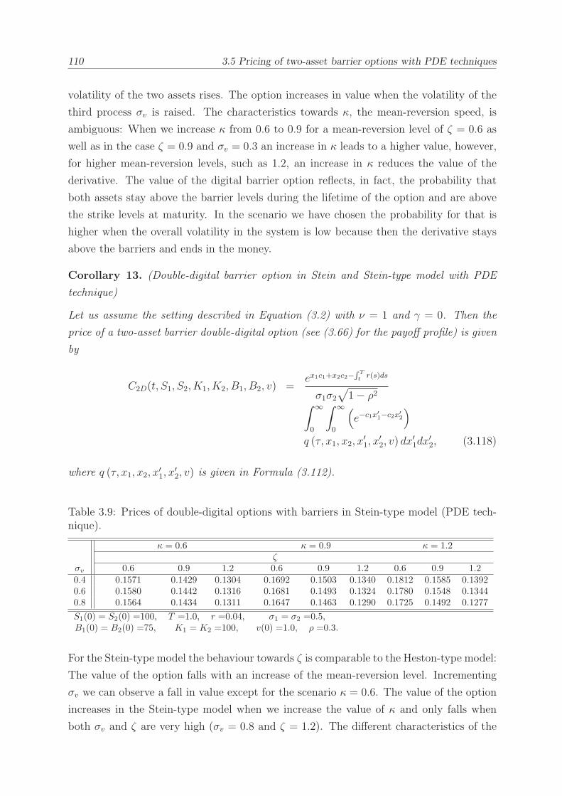
110 3.5 Pricing of two-asset barrier options with PDE techniques
volatility of the two assets rises. The option increases in value when the volatility of the
third process σv is raised. The characteristics towards κ, the mean-reversion speed, is
ambiguous: When we increase κ from 0.6 to 0.9 for a mean-reversion level of ζ = 0.6 as
well as in the case ζ = 0.9 and σv = 0.3 an increase in κ leads to a higher value, however,
for higher mean-reversion levels, such as 1.2, an increase in κ reduces the value of the
derivative. The value of the digital barrier option reflects, in fact, the probability that
both assets stay above the barrier levels during the lifetime of the option and are above
the strike levels at maturity. In the scenario we have chosen the probability for that is
higher when the overall volatility in the system is low because then the derivative stays
above the barriers and ends in the money.
Corollary 13. (Double-digital barrier option in Stein and Stein-type model with PDE
technique)
Let us assume the setting described in Equation (3.2) with ν = 1 and γ = 0. Then the
price of a two-asset barrier double-digital option (see (3.66) for the payoff profile) is given
by
C2D(t, S1, S2, K1, K2, B1, B2, v) =ex1c1+x2c2−
∫ Tt
r(s)ds
σ1σ2√
1− ρ2∫ ∞
0
∫ ∞
0
(
e−c1x′1−c2x
′2
)
q (τ, x1, x2, x′1, x
′2, v) dx
′1dx
′2, (3.118)
where q (τ, x1, x2, x′1, x
′2, v) is given in Formula (3.112).
Table 3.9: Prices of double-digital options with barriers in Stein-type model (PDE tech-nique).
κ = 0.6 κ = 0.9 κ = 1.2ζ
σv 0.6 0.9 1.2 0.6 0.9 1.2 0.6 0.9 1.20.4 0.1571 0.1429 0.1304 0.1692 0.1503 0.1340 0.1812 0.1585 0.13920.6 0.1580 0.1442 0.1316 0.1681 0.1493 0.1324 0.1780 0.1548 0.13440.8 0.1564 0.1434 0.1311 0.1647 0.1463 0.1290 0.1725 0.1492 0.1277
S1(0) = S2(0) =100, T =1.0, r =0.04, σ1 = σ2 =0.5,B1(0) = B2(0) =75, K1 = K2 =100, v(0) =1.0, ρ =0.3.
For the Stein-type model the behaviour towards ζ is comparable to the Heston-type model:
The value of the option falls with an increase of the mean-reversion level. Incrementing
σv we can observe a fall in value except for the scenario κ = 0.6. The value of the option
increases in the Stein-type model when we increase the value of κ and only falls when
both σv and ζ are very high (σv = 0.8 and ζ = 1.2). The different characteristics of the

3 Pricing of barrier options within stochastic covariance model 111
Heston and the Stein model can be explained by the different form of the diffusion term
of the third factor process: The diffusion in the former model depends on√vσv while the
diffusion of the later only depends on σv.
3.5.3 Pricing of two-asset barrier correlation options with PDE
techniques
In the following we derive formulas to price two-asset barrier correlation options with
time-dependent barriers.
Corollary 14. (Correlation barrier option in Heston-type model with PDE technique)
Let us assume the setting described in Equations (3.2) and (3.3) with ν = γ = 12. Then
the price of a two-asset barrier correlation option (see (3.70) for the payoff profile) is
given by
C2C(t, S1, S2, K1, K2, B1, B2, v) =ex1c1+x2c2−
∫ Tt
r(s)ds
σ1σ2√
1− ρ2K1K2
∫ ∞
0
∫ ∞
0
(
ex′1(1−c1) − e−x′
1c1
)
(
ex′2(1−c2) − e−x′
2c2
)
q (τ, x1, x2, x′1, x
′2, v) dx
′1dx
′2, (3.119)
where q (τ, x1, x2, x′1, x
′2, v) is given in Formula (3.110).
Table 3.10: Prices of correlation options with barriers in Heston-type model (PDE tech-nique).
κ = 0.6 κ = 0.9 κ = 1.2ζ
σv 0.6 0.9 1.2 0.6 0.9 1.2 0.6 0.9 1.20.4 313.87 326.25 337.69 307.90 325.27 340.85 302.73 324.43 343.400.6 310.23 322.84 334.50 304.80 322.43 338.27 300.08 322.05 341.280.8 305.52 318.31 330.21 300.76 318.64 334.76 296.62 318.85 338.38
S1(0) = S2(0) =100, T =1.0, r =0.04, σ1 = σ2 =0.5,B1(0) = B2(0) =75, K1 = K2 =100, v(0) =1.0, ρ =0.
Again, we first compare prices computed using the Fourier technique (see Section 3.4.4)
with the prices computed with PDE-based formulas. In Table 3.10 it can be seen that
the results are quite close to Table 3.5. For the correlation option the picture is different.
The payoff of this derivative is not only influenced by the probability that the underlyings
stay above the barriers during lifetime and above the strike levels at maturity but also by
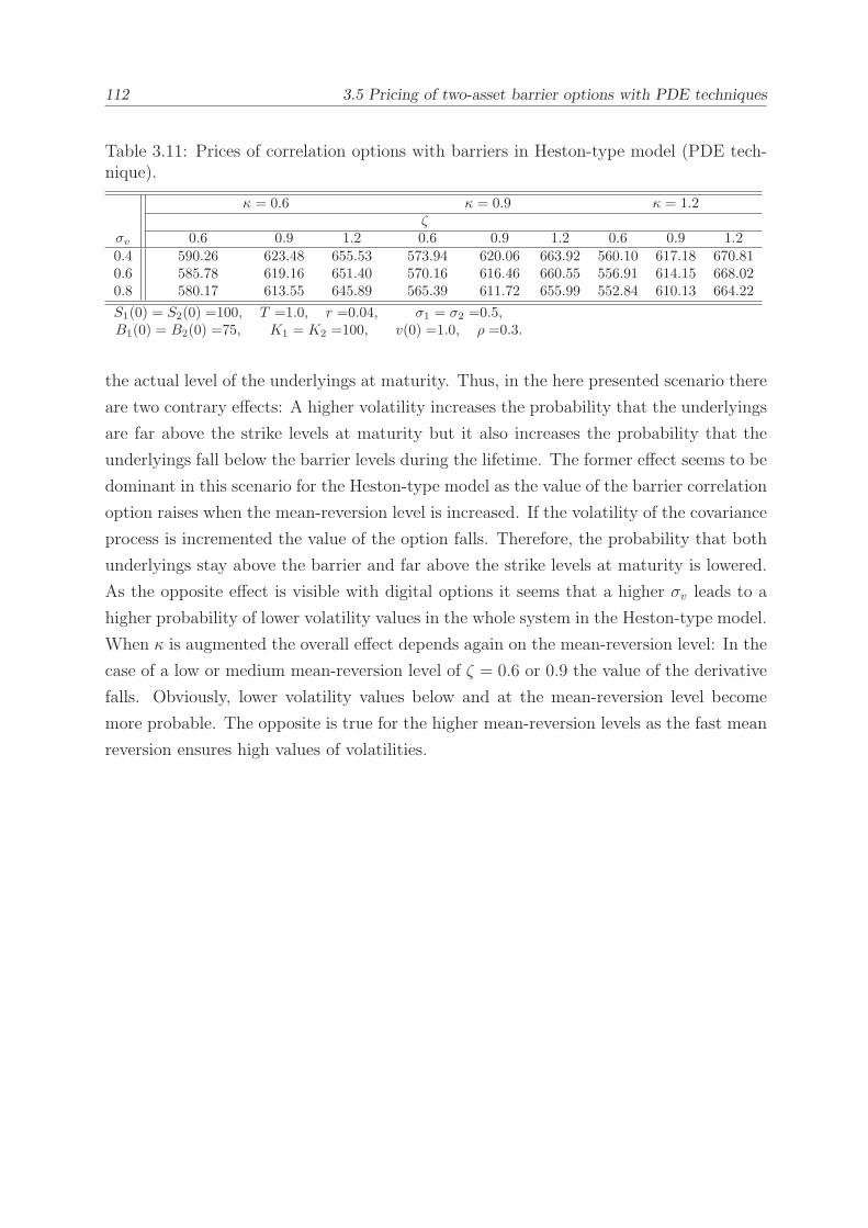
112 3.5 Pricing of two-asset barrier options with PDE techniques
Table 3.11: Prices of correlation options with barriers in Heston-type model (PDE tech-nique).
κ = 0.6 κ = 0.9 κ = 1.2ζ
σv 0.6 0.9 1.2 0.6 0.9 1.2 0.6 0.9 1.20.4 590.26 623.48 655.53 573.94 620.06 663.92 560.10 617.18 670.810.6 585.78 619.16 651.40 570.16 616.46 660.55 556.91 614.15 668.020.8 580.17 613.55 645.89 565.39 611.72 655.99 552.84 610.13 664.22
S1(0) = S2(0) =100, T =1.0, r =0.04, σ1 = σ2 =0.5,B1(0) = B2(0) =75, K1 = K2 =100, v(0) =1.0, ρ =0.3.
the actual level of the underlyings at maturity. Thus, in the here presented scenario there
are two contrary effects: A higher volatility increases the probability that the underlyings
are far above the strike levels at maturity but it also increases the probability that the
underlyings fall below the barrier levels during the lifetime. The former effect seems to be
dominant in this scenario for the Heston-type model as the value of the barrier correlation
option raises when the mean-reversion level is increased. If the volatility of the covariance
process is incremented the value of the option falls. Therefore, the probability that both
underlyings stay above the barrier and far above the strike levels at maturity is lowered.
As the opposite effect is visible with digital options it seems that a higher σv leads to a
higher probability of lower volatility values in the whole system in the Heston-type model.
When κ is augmented the overall effect depends again on the mean-reversion level: In the
case of a low or medium mean-reversion level of ζ = 0.6 or 0.9 the value of the derivative
falls. Obviously, lower volatility values below and at the mean-reversion level become
more probable. The opposite is true for the higher mean-reversion levels as the fast mean
reversion ensures high values of volatilities.
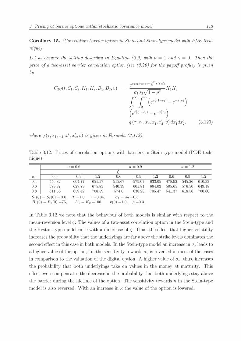
3 Pricing of barrier options within stochastic covariance model 113
Corollary 15. (Correlation barrier option in Stein and Stein-type model with PDE tech-
nique)
Let us assume the setting described in Equation (3.2) with ν = 1 and γ = 0. Then the
price of a two-asset barrier correlation option (see (3.70) for the payoff profile) is given
by
C2C(t, S1, S2, K1, K2, B1, B2, v) =ex1c1+x2c2−
∫ Tt
r(s)ds
σ1σ2√
1− ρ2K1K2
∫ ∞
0
∫ ∞
0
(
ex′1(1−c1) − e−x′
1c1
)
(
ex′2(1−c2) − e−x′
2c2
)
q (τ, x1, x2, x′1, x
′2, v) dx
′1dx
′2, (3.120)
where q (τ, x1, x2, x′1, x
′2, v) is given in Formula (3.112).
Table 3.12: Prices of correlation options with barriers in Stein-type model (PDE tech-nique).
κ = 0.6 κ = 0.9 κ = 1.2ζ
σv 0.6 0.9 1.2 0.6 0.9 1.2 0.6 0.9 1.20.4 556.82 604.77 651.57 515.67 575.07 633.05 478.92 545.26 610.330.6 579.87 627.79 675.83 540.39 601.81 664.02 505.65 576.50 649.180.8 611.56 659.42 708.59 574.0 638.28 705.47 541.37 618.56 700.60
S1(0) = S2(0) =100, T =1.0, r =0.04, σ1 = σ2 =0.5,B1(0) = B2(0) =75, K1 = K2 =100, v(0) =1.0, ρ =0.3.
In Table 3.12 we note that the behaviour of both models is similar with respect to the
mean-reversion level ζ: The values of a two-asset correlation option in the Stein-type and
the Heston-type model raise with an increase of ζ. Thus, the effect that higher volatility
increases the probability that the underlyings are far above the strike levels dominates the
second effect in this case in both models. In the Stein-type model an increase in σv leads to
a higher value of the option, i.e. the sensitivity towards σv is reversed in most of the cases
in comparison to the valuation of the digital option. A higher value of σv, thus, increases
the probability that both underlyings take on values in the money at maturity. This
effect even compensates the decrease in the probability that both underlyings stay above
the barrier during the lifetime of the option. The sensitivity towards κ in the Stein-type
model is also reversed: With an increase in κ the value of the option is lowered.

114 3.5 Pricing of two-asset barrier options with PDE techniques
3.5.4 Conclusion
We have found a closed-form expression to price two-asset barrier options. Those options
have a payout at maturity time T , which may depend on S1(T ) and S2(T ) provided that
not any of the two assets crossed a predefined barrier. Closed-form expressions for barrier
options on two assets are rare. He et al. [64] and Zhou [123], [124] presented closed-
form pricing of those derivatives in the context of constant covariance. We extend their
result by allowing for a third factor in the model which governs the covariance of the two
underlyings. The solution found in Theorem 36 is true for any correlation −1 ≤ ρ ≤ 1
between the underlyings, and the implementation is numerically stable. Moreover, we
derive the joint survival probability of the two assets. In some scenario calculations we
analyse the impact of the model parameters on the price of two-asset barrier correlation
and digital options. From our proof of the general pricing formula with PDE techniques, it
is also clear that the assumption that the covariance process and the underlying processes
are independent cannot be relaxed. For those frameworks a closed-form solution is not
possible. Thus, we deal with approximation techniques in the next chapter. There we
also relax the assumption that the covariance is only driven by one common factor. We
rather assume several drivers and even set the correlation stochastic.
In the following we apply the techniques derived in this chapter to the pricing of certificates
under issuer risk. Certificates are retail products which consist of simpler internal hedging
derivatives.

3 Pricing of barrier options within stochastic covariance model 115
3.6 Pricing certificates under issuer risk
3.6.1 Introduction
Since market introduction in 1989, certificates have become very popular with retail cus-
tomers in Germany. In the years 2002 to 2007, the market volume doubled every year
[120], peaking in an all time high of 139 billion EUR at the end of the 3rd quarter of 2007.
In the financial market crisis, the market volume began to decline. Following the filing of
Chapter 11 of Lehman brothers in September 2008, the market for certificates dropped
by 30 billion EUR in one quarter to 80 billion EUR. Until the end of March 2010, the
market in Germany recovered to 106 billion EUR [34].
Certificate are also referred to as structured products. The simplest structures are index
certificates which allow a retail customer to directly invest in an index like the German
stock index Deutscher Aktien Index (DAX) or the Dow Jones Euro Stoxx 50. From a
legal point of view those products are bonds and the investors are, thus, creditors of the
respective issuer. This rather technical aspect has been disregarded in the investment
decision by many retail investors. Even the Value at Risk figures which are sometimes
given by banks as an indicator of the risk involved in single certificates are based on the
assumption of a non-defaultable issuer. However, in the case of an insolvency of the issuer
the investor may lose his total investment regardless of the performance of the underlyings
of the certificate. The case of Lehman Brothers shows that this risk can in fact materialise.
Certificates differ in this feature from an investment in funds. The investment in a fund
is a so-called special property and is not affected at all by the creditworthiness of the
issuing company because the fund is protected against the bankruptcy of the issuer.
Issuer risk is the risk of loss on securities and other tradeable obligations because the
issuer does not fulfil his contractual obligations due to his insolvency. Up to today this
kind of risk has hardly been addressed in the pricing of exotic securities and especially not
from a retailer’s perspective but only in connection with regulatory capital requirements,
e.g. Basel II. More details about modelling and evaluating counterparty/issuer risk under
an economic or regulatory perspective can be found in [17], [97], [98].
Pricing securities under counterparty risk can be traced back to Merton [87]. Johnson
and Stulz [74] analysed the counterparty risk in option pricing. They used a firm value
model and assumed that the vulnerable option presents the single debt of the company.
A huge increase in the derivative’s value, thus, rises the risk of default of the company.
This approach is only appropriate when the derivative is the only or the predominant
source of funding of the counterparty. Hull and White [69] as well as Jarrow and Turnbull
[72] value so-called vulnerable options, options on a bond written by a defaultable party,
116 3.6 Pricing certificates under issuer risk
in a reduced form model. They assume independence between the credit risk of the
counterparty and the asset underlying the derivative. Cherubini and Luciano (see [20],
[21]) suggest to use a copula approach to value the counterparty risk in an investment.
This allows to model a dependence structure between term-structure movements and a
default of one of the parties.
Klein [78] as well as Klein and Inglis [79] choose a firm-value model to account for the
issuer risk and to model the dependencies between the issuing firm and the underlying.
We follow their approach in that regard, and condition the payoff of the certificate on
the survival of the issuer: The certificate only pays the total investment and gains back
as long as the issuer has not defaulted, i.e. its asset value has not fallen under a certain
barrier.
Like Klein [78] and Klein and Inglis [79] we model the correlation between the assets of
the issuer and the asset underlying the derivative explicitly. The barrier is exponentially
increasing in time. The issuer can default any time before maturity. In the case of default
the investor recovers a constant fraction of the market value of his investment. As we deal
with retail products we furthermore assume that the exotic structures are fully hedged,
i.e. all debt owed to the investor has to be seen alongside assets which the company owns.
In the case of default, however, these assets do not cover the claims of the investors but are
part of the insolvency estate. This allows us to assume the boundary as deterministically
increasing rather than stochastic (see [79]).
3.6.2 The model
The model formulation is influenced by the CreditGrades framework (for details see [110]
and [107]). This approach allows us to derive closed-form expressions for index, partici-
pation guarantee, bonus guarantee, discount, and bonus certificates under issuer risk in a
Black-Scholes and a stochastic covariance framework.
The system of processes is defined on a filtered probability space (Ω,F , Q,F). We as-
sume the existence of an equivalent martingale measure. As an immediate consequence
the market is arbitrage-free. The processes are directly formulated under the martingale
measure Q. We consider an issuing company i = 1 with an asset value per share at time t
of V1(t), an equity price S1(t), and a total debt per share of D1(t). The firm’s asset value
dynamics follow a geometric Brownian motion
dV1V1
= (r − d1)dt+ σ1dW1, V1(0) = S1(0) +D1(0), (3.121)
3 Pricing of barrier options within stochastic covariance model 117
or a process with stochastic volatility, respectively
dV1V1
= (r − d1)dt+ σ1vνdW1, V1(0) = S1(0) +D1(0), (3.122)
where r is the risk-free interest rate and d1 is the dividend yield on the company’s assets.
Both processes, r and d1, are assumed deterministic. v is driven by a stochastic process
dv = κ(ζ − v)dt+ σvvγdZ, (3.123)
〈dW1, dZ〉 = 0,
and ν, κ, ζ, σv, and γ are constants. The company’s debt is deterministic and yields a
continuous interest of r(s)− d1(s).
D1(t) = D1(0)e∫ t0 (r(s)−d1(s))ds. (3.124)
The issuing company defaults if its asset value falls below that barrier D1(t). Thus, the
time of default is defined by the stopping time ι′1
ι′1 = inf t′ ∈ (t0, T ] : V1(t′) < D1(t
′) . (3.125)
We denote the equity per share by
S1(t) = V1(t)−D1(t), if ι1 > t and,
S1(t) = 0 otherwise.(3.126)
This implies that default occurs whenever the stock price S1(t) falls to zero. As soon as
S1(t) reaches zero it remains there. In this framework an European option is seen as the
corresponding down-and-out barrier option with an absorbing barrier for S1(t) set at 0.
Hence, an equivalent time to default to ι′1 is
ι1 = inf t′ ∈ (t0, T ] : S1(t′) ≤ 0 . (3.127)
In the GBM framework the dynamics for S1(t) are, prior to default, found by applying
Ito to (3.126) and are given by
dS1 = S1(r − d1)dt+ (D1(t) + S1)σ1dW1. (3.128)
The stock price of the issuer follows – prior to default – a shifted log-normal distribution.
This distribution implies negative stock prices with positive probability (see [107] for more
details): The higher the leverage (debt-to-equity ratio) the higher is the probability of
118 3.6 Pricing certificates under issuer risk
default and vice versa.
The dynamics of the underlying assets of a certificate are modelled by geometric Brownian
motions. The following system is considered to describe the assets of the issuer and the
underlying assets of the derivatives:
dS1 = S1(r − d1)dt+ (D1(t) + S1)σ1dW1, (3.129)
dSi = Si(r − di)dt+ SiσidWi for i = 2, . . . , d,
〈dWi, dWk〉 = ρikdt,
where σi and ρ are constants (see [67]).
This framework is compared to a stochastic covariance framework, where S1 is modelled
by
dS1 = S1(r − d1)dt+ (D1(t) + S1)σ1vνdW1, (3.130)
where v is driven by (3.131). Hence, the framework is given by
dS1 = S1(r − d1)dt+ (D1(t) + S1)σ1vνdW1, (3.131)
dSi = Si(r − di)dt+ SiσivνdWi for i = 2, . . . , d,
dv = κ(ζ − v)dt+ σvvγdZ, (3.132)
〈dWi, dZ〉 = 0,
〈dWi, dWk〉 = ρikdt.
In the following we consider the Heston-type model with ν = γ = 12and the Stein-type
model with ν = 1 and γ = 0.
3.6.3 Pricing of certificates under issuer risk
Building blocks
The most popular certificates are composed from simple building blocks such as zero-
coupon bonds CZ(t), investments in an underlying S2(t), call options CCall (t, S2, K2),
and digital options CD (t, S2, K2) as well as knock-out put options C1P (t, S2, K2, B2).
The formulas for these components are derived for the case that the issuer can default
and has a recovery rate of zero (for a similar model see [83], p. 635ff). In the case of no
default the valuation of the building blocks is well-known and will be provided for the
purpose of completeness. By means of these building blocks defaultable index, guarantee,
and bonus certificates can be valued for any assumption of the recovery rate. The proofs
3 Pricing of barrier options within stochastic covariance model 119
for the results in this section will be provided in the Appendix A.2.
A main component of index certificates and discount certificates is the investment in the
underlying S2, which is actually worth S2(t) at time t, when we assume that the issuer
cannot default. However, when we suppose that the investor does not obtain the dividends
paid out the value is given by S2(t)e−∫ Tt
d2(s)ds.
Proposition 4. (Investment in a stock)
In the case when the investment in the equity is guaranteed by an issuer who is defaultable
with recovery rate zero, the price SD2,t of this investment in Model (3.129) at time t is given
by
CDS = S2e
−∫ Tt
d2(s)ds(
N (d1)
− exp2x∗1(c1 − ρ
σ2σ1
(1− c2))N(
d1
))
,
where N2(x, y, ρ) is the standard bivariate normal distribution function with correlation
ρ,
x∗1 = ln(S1 +D1(t)
D1(t)), x2 = ln
(
S2e∫ Tt(r(s)−d2(s))ds
)
,
τ = T − t,
c1 =σ1 − ρσ2
2σ1(1− ρ2), c2 =
σ2 − ρσ12σ2(1− ρ2)
,
d1 =x∗1
σ1√τ− 1
2σ1√τ + ρσ2
√τ , d1 = −
x∗1σ1√τ− 1
2σ1√τ + ρσ2
√τ .
In the stochastic covariance Framework (3.131) the price is given by
CDS (t, S1, S2, v) =
ex∗1c1+x2c2−
∫ Tt
r(s)ds
2πσ1
∫ i1+∞
i1−∞
˜hCD
S(u1)
(ϕ (τ,u,−z1,−z2, v)− ϕ (τ,u, z1,−z2, v)) du1,u ∈ SCD
S= Sϕ ∩ Sg
CDS
,
where
˜hDS (u1, u2) =
(
−1iu1
σ1+ ρσ2(1−c2)
σ1− c1
)
,
with ℑ(u1) = 1 > −σ1c1 + (1 − c2)σ2ρ, i.e. SgCDS
=
u = w + i : 2 = 0 ∧1 > −σ1c1 + (1− c2)σ2ρ and the characteristic functions

120 3.6 Pricing certificates under issuer risk
ϕ(τ,u, z, v) for the Heston-type and the Stein and Stein-type models are given by
ϕH(τ,u, z, v) = exp
iu1z1 + iu2z2 +1
σ2v
(AH(τ,u) + BH(τ,u)v)
, (3.133)
ϕS2(τ,u, z, v) = exp
iu1z1 + iu2z2 +1
σ2v
(AS2(τ,u) + BS2(τ,u)v + CS2(τ,u)v
2)
,
with AH , BH , AS2, BS2, and CS2 as defined in (3.48)-(3.49) and (3.59)-(3.61).
For a proof see A.2.2.
Products, which ensure a repayment of an investment with notional 1 at maturity, are
internally stripped into a zero-coupon bond and several derivatives. As known, a non-
defaultable zero-coupon bond is priced by CZ(t) = e−∫ Tt
r(s)ds.
Proposition 5. (Zero-coupon bond)
When we assume that the issuer can default and – if he defaults – he does so with no
recovery, the value of the zero-coupon bond in the GBM framework can be computed by
(see [107])
CDZ (t) = e−
∫ Tt
r(s)ds(
N (d∗1)− ex
∗1N(
d∗1
))
, (3.134)
with N (.) being the standard cumulative normal distribution function, and
d∗1 =
x∗1σ1√τ− 1
2σ1√τ , d∗
1 = −x∗1
σ1√τ− 1
2σ1√τ .
When the issuer additionally promises a fixed interest rI on the investment this is valued,
assuming no default, by CDZ (t, I) = (1 + rI) e
−∫ Tt
r(s)ds and accordingly by CDZ (t, I) =
e−∫ Tt
r(s)ds (1 + rI)(
N (d∗1)− ex
∗1N(
d∗1
))
in a world with defaults and zero recovery.
In the stochastic covariance framework with defaults the zero bond is priced by (see [107])
CDZ (t, S1, v) =
e12x∗1−∫ Tt
r(s)ds
2π
∫ ∞
−∞
ϕ(τ, u1, x∗1, v)− ϕ(τ, u1,−x∗1, v)iu1 − 1
2
du1, (3.135)
where the one-dimensional characteristic functions for the Heston-type model and the
Stein-type model are given by
ϕH(τ, u, v) = exp
iu1x∗1 +
1
σ2v
(AH(τ, u1) + BH(τ, u1)v)
, (3.136)
ϕS2(τ, u, v) = exp
iu1x∗1 +
1
σ2v
(AS2(τ, u1) + BS2(τ, u1)v + CS2(τ, u1)v
2)
,
3 Pricing of barrier options within stochastic covariance model 121
where
d = d(u1) =
√
κ2 + σ2vσ
2
(
u12 +1
4
)
,
and with AH , BH , AS2, BS2, and CS2 as defined in (3.48)-(3.49) and (3.59)-(3.61).
Call options are introduced in the structured products to leverage the investment and
to grant the investor a high participation rate in the returns of the underlying. In
the GBM framework with a non-defaultable issuer the call option with strike K2 is
priced by the well-known Black-Scholes formula CCall (t, S2, K2) = S2e∫ Tt
r(s)dsN (d2) −K2e
−∫ Tt
r(s)dsN (d∗2), where d2 =
x2
σ2√τ+ 1
2σ2√τ , x2 =
S2e∫Tt (r(s)−d2(s))ds
K2and d∗
2 = d2−σ2√τ .
In the stochastic covariance framework the call price is given by CCall(t, S2, K2, v) =K2e
12x2−
∫Tt r(s)ds
2π
(
2πe12x2 −
∫∞−∞
ϕ(τ,u2,−x2,v)
u22+
14
)
(see [107]).
Proposition 6. (Call option)
In the GBM Framework (3.129) at time t the price CDC (t, S1, S2, K2) of a defaultable call
option, when the payment of the call option is guaranteed by an issuer who is defaultable
with recovery rate zero, is given by
CDCall(t, S1, S2, K2) =
((
S2e−∫ Tt
d2(s)dsN2 (d1,d2, ρ)−K2e−∫ Tt
r(s)dsN2 (d∗1,d
∗2, ρ)
)
−(
S2e−∫ Tt
d2(s)ds exp
2x∗1(c1 − (1− c2)σ2ρ
σ1)
N2
(
d1, d2, ρ)
−K2e−∫ Tt
r(s)ds exp
2x∗1(c1 + c2σ2ρ
σ1)
N2
(
d∗1, d
∗2, ρ)))
,
where x∗1, x2, c1, c2, as well as d1, and d1 are given in Proposition 4,
d2 = x2
σ2√τ+ 1
2σ2√τ , d2 =
x2σ2√τ− 2ρ
x∗1σ1√τ+
1
2σ2√τ ,
d∗1 = d1 − ρσ2
√τ , d∗
2 = d2 − σ2√τ ,
d∗1 = d1 − ρσ2
√τ , d∗
2 = d2 − σ2√τ .
In the stochastic covariance Framework (3.131) the price is given by
CDCall(t, S1, S2, v) =
ex∗1c1+x2c2−
∫ Tt
r(s)ds
4π2σ1σ2√
1− ρ2∫ i2+∞
i2−∞
∫ i1+∞
i1−∞hCD
Call(u1)
(ϕ (τ,u,−z1,−z2, v)− ϕ (τ,u, z1,−z2, v)) du1du2,u ∈ SCD
Call= Sϕ ∩ Sg
CDCall
,

122 3.6 Pricing certificates under issuer risk
where
hDC (u1, u2) = K21
i
(
u1
σ1− u2ρ
σ1
√1−ρ2
)
− c1
1(
i u2
σ2
√1−ρ2
+ 1− c2)(
i u2
σ2
√1−ρ2− c2
) .
Note that we have to set ℑ(u2) > σ2√
1− ρ2(1 − c2) and ℑ(u1) > ρ√1−ρ2ℑ(u2) − σ1c1,
i.e. SgDC=
u = w + i : 2 > σ2√
1− ρ2(1− c2) ∧1 >ρ√1−ρ2
2 − σ1c1
. The char-
acteristic functions for the Heston-type and the Stein and Stein-type models are as given
in Proposition 4.
For a proof see A.2.2.
Similarly in the GBM framework, the non-defaultable digital option with strike K2 is
priced by CD(t, S2, K2) = e−∫ Tt
r(s)dsN(d∗2) and in the stochastic covariance model by
CD(t, S2, K2, v) =e12x2−
∫Tt r(s)ds
2π
∫∞−∞
ϕ(τ,u2,−x2,v)12−iu2
.
Proposition 7. (Digital option)
In the GBM Model (3.129) at time t the price CDD (t, S1, S2, K2) of a defaultable digital
call option, when the payment of one is guaranteed by an issuer who is defaultable with
recovery rate zero, is given by
CDD (t, S1, S2, K2) = e−
∫ Tt
r(s)ds
(
N2 (d∗1,d
∗2, ρ)− exp
2x∗1(c1 + c2σ2ρ
σ1)
N2
(
d∗1, d
∗2, ρ))
,
where x∗1, x2, c1, c2, d∗1, and d∗
1 are given in Proposition 4, d∗2 and d∗
2 are defined in
Proposition 6.
In the stochastic covariance Framework (3.131) with defaults the price is given by
CDD (t, S1, S2, K2, v) =
ex∗1c1+x2c2−
∫ Tt
r(s)ds
4π2σ1σ2√
1− ρ2∫ i2+∞
i2−∞
∫ i1+∞
i1−∞hCD
D(u1)
(ϕ(τ,u,−z1,−z2, v)− ϕ(τ,u, z1,−z2, v)) du1du2,u ∈ SCD
D= Sϕ ∩ Sg
CDD
,
where
hDD(u1, u2) =1
iu2
σ2
√
1− ρ2 − c21
i
(
u1
σ1− ρ u2
σ2
√1−ρ2
)
− c1,

3 Pricing of barrier options within stochastic covariance model 123
with ℑ(u2) > −σ2√
1− ρ2c2 and ℑ(u1) > ρ√1−ρ2ℑ(u2)− σ1c1, i.e. SgDC
= u = w + i :
2 > −σ2√
1− ρ2c2 ∧ 1 > ρ√1−ρ2
2 − σ1c1 . The characteristic functions for the
Heston-type and the Stein and Stein-type models are as given in Proposition 4.
For a proof see A.2.2.
The bonus certificate includes, beside other derivatives, a knock-out put option. The
price of a non-defaultable knock-out put option with barrier B2(t) = B2e∫ t0 (r(s)−d2(s))ds
and strike K2 is given by (see also [64])
C1P (t, S1, S2, K2, B2) = CP (t, S2, K2)
−e−∫ Tt
d2(s)dsB2
N(2b2 − x2σ2√τ− 1
2σ2√τ
)
+Se−∫ Tt
r(s)dsK2
B2
N(
2b2 − x2σ2√T − t +
1
2σ2√τ
)
,
where
CP (t, S2, K2) = K2e−∫ Tt
r(s)dsN(
−d2
)
− S2e−∫ Tt
d2(s)dsN(
−d1
)
,
x2 = ln(S2e
∫ Tt(r(s)−d2(s))ds
K2
), b2 = ln (B2(T )
K2
).
In the stochastic covariance framework the default-free price is given by
C1P (t, S2, K2, B2, v) = −K2e− 1
2x2−
∫ Tt
r(s)ds
2π
∫ ∞
−∞(ϕ(τ, u2,−x2, v)− ϕ(τ, u2, x2 − 2b, v))
1 + eib2u2
((iu2 − 1
2
)e
b22 −
(iu2 − 1
2
)e−
b22
)
u22 +14
du2, (3.137)
where the one-dimensional characteristic functions are given in (3.136). For a proof see
[39].
124 3.6 Pricing certificates under issuer risk
Proposition 8. (Barrier option)
In the GBM Model (3.129) the price CD1P (t, S1, S2, K2, B2) of a defaultable knock-out put
option at time t, when the payoff is guaranteed by an issuer who is defaultable with recovery
rate zero, is given by
CD1P (t, S1, S2, K2, B2) =
K2ec1x
∗1+c2x2−
∫ Tt
r(s)ds
σ1σ2√
1− ρ2∫ ∞
0
∫ 0
−∞e−c1x
∗1′(
e−c2x′2 − e(1−c2)x2
)
pGBM(τ, x∗1′, x′2, x
∗1, x2)dx
∗1′dx′2, (3.138)
where y1 =x∗1
σ1, y2 =
x2
σ2, and
pGBM(τ, x∗1′, x′2, x
∗1, x2) =
2e−ατ
βpτ
∞∑
n=1
e−(r2p+r′p
2)
2τ sinnπθ′pβp
sinnπθpβp
Inπβp
(r′prp
τ
)
,
tan βp = −√
1− ρ2ρ
, β ∈ [0, π] ,
rp =
√
1
(1− ρ2)
(x∗1σ1− ρx2
σ2
)2
+
(x2σ2
)2
,
tan(θp) =x2
σ2
1√1−ρ2
(x∗1
σ1− ρx2
σ2
) , θp ∈ [0, βp] . (3.139)
In the stochastic covariance framework with defaults the respective formulas were derived
in Section 3.5.1. Hence,
CD1P (t, S1, S2, K2, B2, v) =
K2ec1x
∗1+c2x2−
∫ Tt
r(s)ds
σ1σ2√
1− ρ2∫ ∞
0
∫ 0
−∞e−c1x
∗1′(e−c2x
′2 − e(1−c2)x2)
q(τ, x∗1′, x′2, x
∗1, x2, v)dx
′2dx
∗1′, (3.140)
where q(τ, x∗1′, x′2, x
∗1, x2, v) is given in (3.91) for the general case, for the Heston-type
model in (3.110) and for the Stein-type model in (3.112).
Index certificates
In this section we price an index certificate with price IC(t) at time t under issuer risk.
As stated before, the index certificate allows a retail investor to invest in a single stock
or stock index with price S2(t) at time t. He fully participates in any movement of the
underlying. The index certificate does not provide any protection against a decline of the
underlying. Internally this certificate is hedged by buying the respective index or single
stock. Taking into consideration the issuer risk and assuming a constant recovery rate R
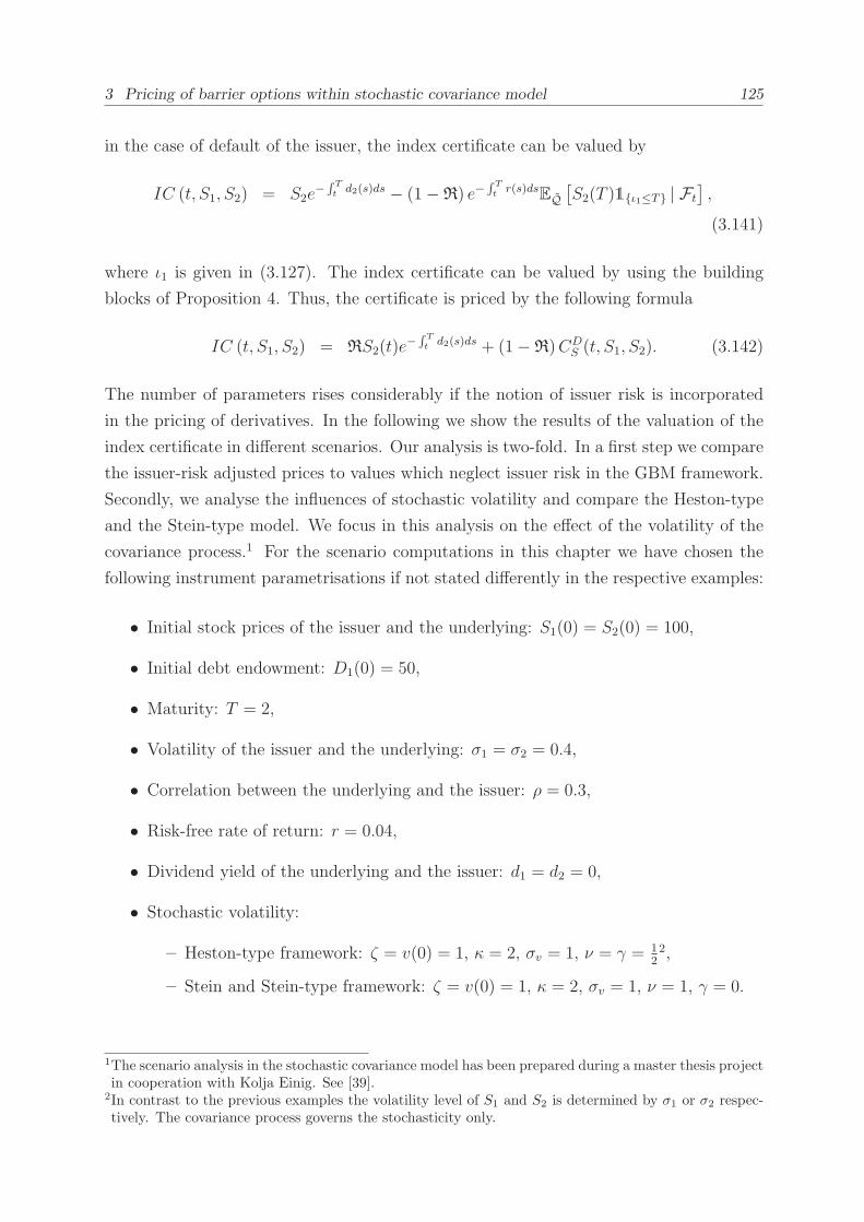
3 Pricing of barrier options within stochastic covariance model 125
in the case of default of the issuer, the index certificate can be valued by
IC (t, S1, S2) = S2e−∫ Tt
d2(s)ds − (1−R) e−∫ Tt
r(s)dsEQ[S2(T )1ι1≤T | Ft
],
(3.141)
where ι1 is given in (3.127). The index certificate can be valued by using the building
blocks of Proposition 4. Thus, the certificate is priced by the following formula
IC (t, S1, S2) = RS2(t)e−∫ Tt
d2(s)ds + (1−R)CDS (t, S1, S2). (3.142)
The number of parameters rises considerably if the notion of issuer risk is incorporated
in the pricing of derivatives. In the following we show the results of the valuation of the
index certificate in different scenarios. Our analysis is two-fold. In a first step we compare
the issuer-risk adjusted prices to values which neglect issuer risk in the GBM framework.
Secondly, we analyse the influences of stochastic volatility and compare the Heston-type
and the Stein-type model. We focus in this analysis on the effect of the volatility of the
covariance process.1 For the scenario computations in this chapter we have chosen the
following instrument parametrisations if not stated differently in the respective examples:
• Initial stock prices of the issuer and the underlying: S1(0) = S2(0) = 100,
• Initial debt endowment: D1(0) = 50,
• Maturity: T = 2,
• Volatility of the issuer and the underlying: σ1 = σ2 = 0.4,
• Correlation between the underlying and the issuer: ρ = 0.3,
• Risk-free rate of return: r = 0.04,
• Dividend yield of the underlying and the issuer: d1 = d2 = 0,
• Stochastic volatility:
– Heston-type framework: ζ = v(0) = 1, κ = 2, σv = 1, ν = γ = 122,
– Stein and Stein-type framework: ζ = v(0) = 1, κ = 2, σv = 1, ν = 1, γ = 0.
1The scenario analysis in the stochastic covariance model has been prepared during a master thesis projectin cooperation with Kolja Einig. See [39].
2In contrast to the previous examples the volatility level of S1 and S2 is determined by σ1 or σ2 respec-tively. The covariance process governs the stochasticity only.
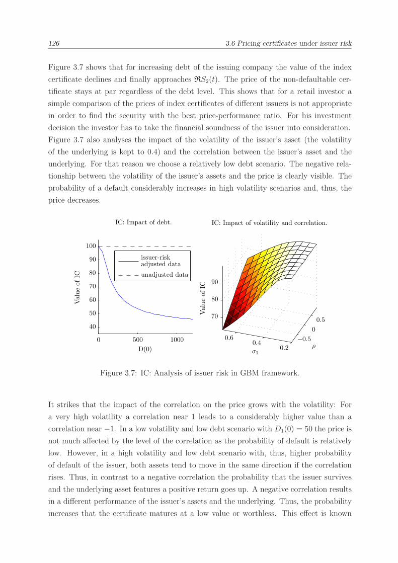
126 3.6 Pricing certificates under issuer risk
Figure 3.7 shows that for increasing debt of the issuing company the value of the index
certificate declines and finally approaches RS2(t). The price of the non-defaultable cer-
tificate stays at par regardless of the debt level. This shows that for a retail investor a
simple comparison of the prices of index certificates of different issuers is not appropriate
in order to find the security with the best price-performance ratio. For his investment
decision the investor has to take the financial soundness of the issuer into consideration.
Figure 3.7 also analyses the impact of the volatility of the issuer’s asset (the volatility
of the underlying is kept to 0.4) and the correlation between the issuer’s asset and the
underlying. For that reason we choose a relatively low debt scenario. The negative rela-
tionship between the volatility of the issuer’s assets and the price is clearly visible. The
probability of a default considerably increases in high volatility scenarios and, thus, the
price decreases.
IC: Impact of volatility and correlation.
Valueof
IC
σ1
ρ
unadjusted data
issuer-riskadjusted data
IC: Impact of debt.
Valueof
IC
D(0)
−0.50
0.5
0 500 10000.2
0.40.6
40
50
60
70
80
90
100
70
80
90
Figure 3.7: IC: Analysis of issuer risk in GBM framework.
It strikes that the impact of the correlation on the price grows with the volatility: For
a very high volatility a correlation near 1 leads to a considerably higher value than a
correlation near −1. In a low volatility and low debt scenario with D1(0) = 50 the price is
not much affected by the level of the correlation as the probability of default is relatively
low. However, in a high volatility and low debt scenario with, thus, higher probability
of default of the issuer, both assets tend to move in the same direction if the correlation
rises. Thus, in contrast to a negative correlation the probability that the issuer survives
and the underlying asset features a positive return goes up. A negative correlation results
in a different performance of the issuer’s assets and the underlying. Thus, the probability
increases that the certificate matures at a low value or worthless. This effect is known
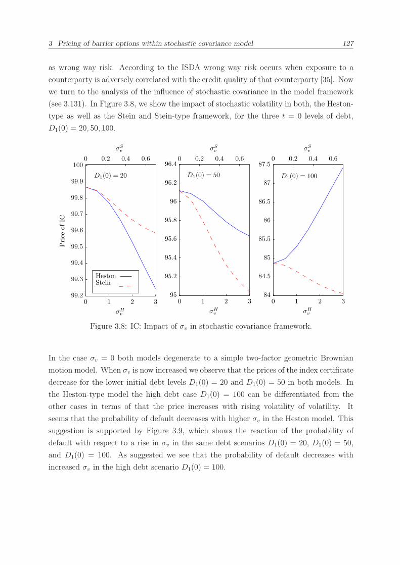
3 Pricing of barrier options within stochastic covariance model 127
as wrong way risk. According to the ISDA wrong way risk occurs when exposure to a
counterparty is adversely correlated with the credit quality of that counterparty [35]. Now
we turn to the analysis of the influence of stochastic covariance in the model framework
(see 3.131). In Figure 3.8, we show the impact of stochastic volatility in both, the Heston-
type as well as the Stein and Stein-type framework, for the three t = 0 levels of debt,
D1(0) = 20, 50, 100.
σSvσS
vσSv
σHvσH
v
Price
ofIC
σHv
HestonStein
D1(0) = 50D1(0) = 20 D1(0) = 100
0 0.2 0.4 0.60 0.2 0.4 0.60 0.2 0.4 0.6
0 1 2 30 1 2 30 1 2 384
84.5
85
85.5
86
86.5
87
87.5
95
95.2
95.4
95.6
95.8
96
96.2
96.4
99.2
99.3
99.4
99.5
99.6
99.7
99.8
99.9
100
Figure 3.8: IC: Impact of σv in stochastic covariance framework.
In the case σv = 0 both models degenerate to a simple two-factor geometric Brownian
motion model. When σv is now increased we observe that the prices of the index certificate
decrease for the lower initial debt levels D1(0) = 20 and D1(0) = 50 in both models. In
the Heston-type model the high debt case D1(0) = 100 can be differentiated from the
other cases in terms of that the price increases with rising volatility of volatility. It
seems that the probability of default decreases with higher σv in the Heston model. This
suggestion is supported by Figure 3.9, which shows the reaction of the probability of
default with respect to a rise in σv in the same debt scenarios D1(0) = 20, D1(0) = 50,
and D1(0) = 100. As suggested we see that the probability of default decreases with
increased σv in the high debt scenario D1(0) = 100.
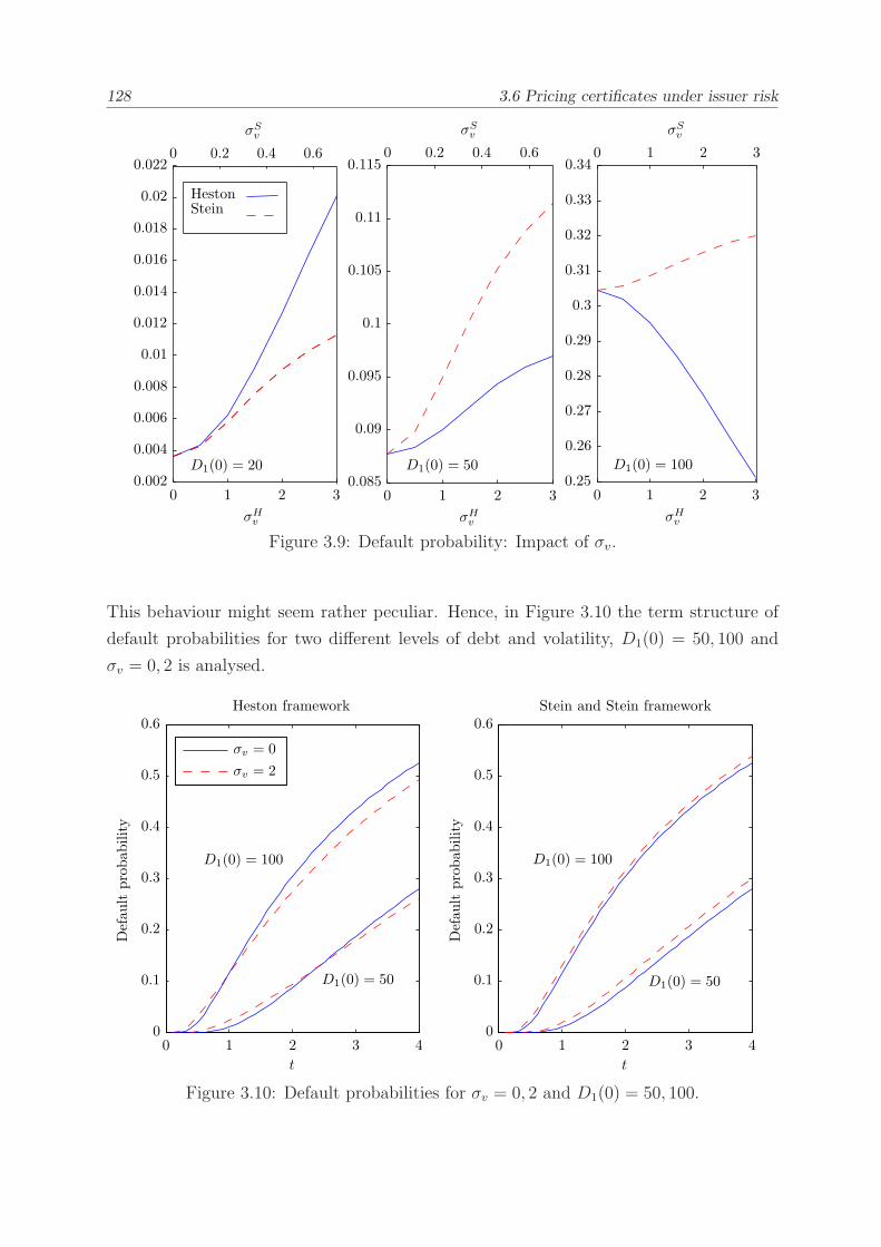
128 3.6 Pricing certificates under issuer risk
σSvσS
vσSv
σHvσH
vσHv
HestonStein
D1(0) = 50 D1(0) = 100D1(0) = 20
0 1 2 30 0.2 0.4 0.60 0.2 0.4 0.6
0 1 2 30 1 2 30 1 2 30.25
0.26
0.27
0.28
0.29
0.3
0.31
0.32
0.33
0.34
0.085
0.09
0.095
0.1
0.105
0.11
0.115
0.002
0.004
0.006
0.008
0.01
0.012
0.014
0.016
0.018
0.02
0.022
Figure 3.9: Default probability: Impact of σv.
This behaviour might seem rather peculiar. Hence, in Figure 3.10 the term structure of
default probabilities for two different levels of debt and volatility, D1(0) = 50, 100 and
σv = 0, 2 is analysed.
Defau
ltprobab
ility
t
Stein and Stein framework
σv = 2
σv = 0
Defau
ltprobab
ility
t
Heston framework
D1(0) = 50
D1(0) = 100 D1(0) = 100
D1(0) = 50
0 1 2 3 40 1 2 3 40
0.1
0.2
0.3
0.4
0.5
0.6
0
0.1
0.2
0.3
0.4
0.5
0.6
Figure 3.10: Default probabilities for σv = 0, 2 and D1(0) = 50, 100.
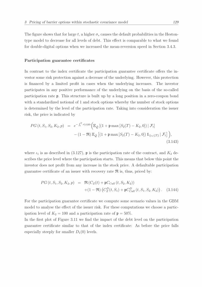
3 Pricing of barrier options within stochastic covariance model 129
The figure shows that for large t, a higher σv causes the default probabilities in the Heston-
type model to decrease for all levels of debt. This effect is comparable to what we found
for double-digital options when we increased the mean-reversion speed in Section 3.4.3.
Participation guarantee certificates
In contrast to the index certificate the participation guarantee certificate offers the in-
vestor some risk protection against a decrease of the underlying. However, this protection
is financed by a limited profit in cases when the underlying increases. The investor
participates in any positive performance of the underlying on the basis of the so-called
participation rate p. This structure is built up by a long position in a zero-coupon bond
with a standardized notional of 1 and stock options whereby the number of stock options
is determined by the level of the participation rate. Taking into consideration the issuer
risk, the price is indicated by
PG (t, S1, S2, K2, p) = e−∫ Tt
r(s)ds(
EQ [(1 + pmax [S2(T )−K2, 0]) | Ft]
− (1−R)EQ[(1 + pmax [S2(T )−K2, 0])1ι1≤T | Ft
] )
,
(3.143)
where ι1 is as described in (3.127), p is the participation rate of the contract, and K2 de-
scribes the price level where the participation starts. This means that below this point the
investor does not profit from any increase in the stock price. A defaultable participation
guarantee certificate of an issuer with recovery rate R is, thus, priced by:
PG (t, S1, S2, K2, p) = R (CZ(t) + pCCall (t, S2, K2))
+(1−R)(CD
Z (t, S1) + pCDCall (t, S1, S2, K2)
). (3.144)
For the participation guarantee certificate we compute some scenario values in the GBM
model to analyse the effect of the issuer risk. For these computations we choose a partic-
ipation level of K2 = 100 and a participation rate of p = 50%.
In the first plot of Figure 3.11 we find the impact of the debt level on the participation
guarantee certificate similar to that of the index certificate: As before the price falls
especially steeply for smaller D1(0) levels.
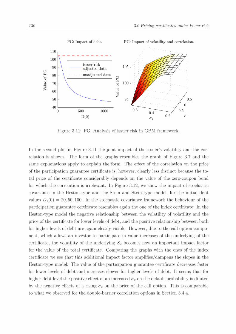
130 3.6 Pricing certificates under issuer risk
PG: Impact of volatility and correlation.
Valueof
PG
σ1
ρ
unadjusted data
issuer-riskadjusted data
PG: Impact of debt.Valueof
PG
D(0)
−0.50
0.5
0 500 10000.2
0.40.6
40
50
60
70
80
90
100
110
95
100
105
Figure 3.11: PG: Analysis of issuer risk in GBM framework.
In the second plot in Figure 3.11 the joint impact of the issuer’s volatility and the cor-
relation is shown. The form of the graphs resembles the graph of Figure 3.7 and the
same explanations apply to explain the form. The effect of the correlation on the price
of the participation guarantee certificate is, however, clearly less distinct because the to-
tal price of the certificate considerably depends on the value of the zero-coupon bond
for which the correlation is irrelevant. In Figure 3.12, we show the impact of stochastic
covariance in the Heston-type and the Stein and Stein-type model, for the initial debt
values D1(0) = 20, 50, 100. In the stochastic covariance framework the behaviour of the
participation guarantee certificate resembles again the one of the index certificate: In the
Heston-type model the negative relationship between the volatility of volatility and the
price of the certificate for lower levels of debt, and the positive relationship between both
for higher levels of debt are again clearly visible. However, due to the call option compo-
nent, which allows an investor to participate in value increases of the underlying of the
certificate, the volatility of the underlying S2 becomes now an important impact factor
for the value of the total certificate. Comparing the graphs with the ones of the index
certificate we see that this additional impact factor amplifies/dampens the slopes in the
Heston-type model: The value of the participation guarantee certificate decreases faster
for lower levels of debt and increases slower for higher levels of debt. It seems that for
higher debt level the positive effect of an increased σv on the default probability is diluted
by the negative effects of a rising σv on the price of the call option. This is comparable
to what we observed for the double-barrier correlation options in Section 3.4.4.
3 Pricing of barrier options within stochastic covariance model 131
σSv σS
vσSv
σHvσH
v
Price
ofPG
σHv
HestonStein
D1(0) = 20 D1(0) = 100D1(0) = 50
0 0.2 0.4 0.6 0 0.2 0.4 0.60 0.2 0.4 0.6
0 1 2 30 1 2 30 1 2 386
86.5
87
87.5
88
88.5
89
98.4
98.6
98.8
99
99.2
99.4
99.6
99.8
100
103
103.5
104
104.5
105
Figure 3.12: PG: Impact of σv.
Bonus guarantee certificates
When investing in a bonus guarantee certificate one does not directly participate in fluc-
tuations of the value of the underlying. Rather, one receives a fixed interest rate and
additionally a bonus payment if the underlying is above the bonus barrier at maturity.
The investor could compose this payoff by buying a zero-coupon bond and a digital option:
BG (t, S1, S2, K2, rI ,Ψ) = e−∫ Tt
r(s)ds(
EQ[(1 + rI +Ψ 1S2(T )>K2
)| Ft
]
−(1−R)EQ[(1 + rI +Ψ 1S2(T )>K2
)1ι1≤T | Ft
] )
,
(3.145)
where ι1 is defined in (3.127), rI the basic interest, Ψ the bonus payment rate, and K2 the
bonus barrier. In our framework the risk-neutral price of the bonus guarantee certificate
is given by
BG (t, S1, S2, K2, rI ,Ψ) = R (CZ(t, I) + Ψ CD (t, S2, K2))
+(1−R)(CD
Z (t, I, S1) + Ψ CDD (t, S1, S2, K2)
).
(3.146)
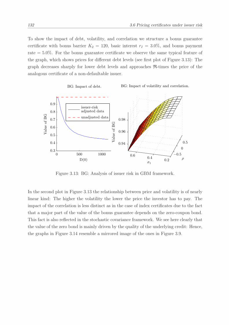
132 3.6 Pricing certificates under issuer risk
To show the impact of debt, volatility, and correlation we structure a bonus guarantee
certificate with bonus barrier K2 = 120, basic interest rI = 3.0%, and bonus payment
rate = 5.0%. For the bonus guarantee certificate we observe the same typical feature of
the graph, which shows prices for different debt levels (see first plot of Figure 3.13): The
graph decreases sharply for lower debt levels and approaches R-times the price of the
analogous certificate of a non-defaultable issuer.
BG: Impact of volatility and correlation.
Valueof
BG
σ1
ρ
unadjusted data
issuer-riskadjusted data
BG: Impact of debt.
Valueof
BG
D(0)
−0.50
0.5
0 500 1000
0.20.4
0.6
0.3
0.4
0.5
0.6
0.7
0.8
0.9
0.94
0.96
0.98
Figure 3.13: BG: Analysis of issuer risk in GBM framework.
In the second plot in Figure 3.13 the relationship between price and volatility is of nearly
linear kind: The higher the volatility the lower the price the investor has to pay. The
impact of the correlation is less distinct as in the case of index certificates due to the fact
that a major part of the value of the bonus guarantee depends on the zero-coupon bond.
This fact is also reflected in the stochastic covariance framework. We see here clearly that
the value of the zero bond is mainly driven by the quality of the underlying credit: Hence,
the graphs in Figure 3.14 resemble a mirrored image of the ones in Figure 3.9.
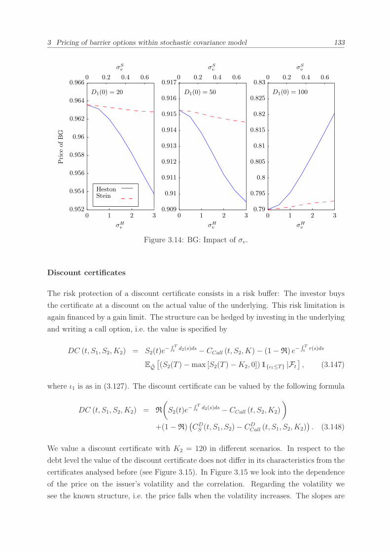
3 Pricing of barrier options within stochastic covariance model 133
σSv σS
vσSv
σHvσH
v
Price
ofBG
σHv
HestonStein
D1(0) = 100D1(0) = 50D1(0) = 20
0 0.2 0.4 0.6 0 0.2 0.4 0.60 0.2 0.4 0.6
0 1 2 30 1 2 30 1 2 30.79
0.795
0.8
0.805
0.81
0.815
0.82
0.825
0.83
0.909
0.91
0.911
0.912
0.913
0.914
0.915
0.916
0.917
0.952
0.954
0.956
0.958
0.96
0.962
0.964
0.966
Figure 3.14: BG: Impact of σv.
Discount certificates
The risk protection of a discount certificate consists in a risk buffer: The investor buys
the certificate at a discount on the actual value of the underlying. This risk limitation is
again financed by a gain limit. The structure can be hedged by investing in the underlying
and writing a call option, i.e. the value is specified by
DC (t, S1, S2, K2) = S2(t)e−∫ Tt
d2(s)ds − CCall (t, S2, K)− (1−R) e−∫ Tt
r(s)ds
EQ[(S2(T )−max [S2(T )−K2, 0])1ι1≤T |Ft
], (3.147)
where ι1 is as in (3.127). The discount certificate can be valued by the following formula
DC (t, S1, S2, K2) = R
(
S2(t)e−∫ Tt
d2(s)ds − CCall (t, S2, K2)
)
+(1−R)(CD
S (t, S1, S2)− CDCall (t, S1, S2, K2)
). (3.148)
We value a discount certificate with K2 = 120 in different scenarios. In respect to the
debt level the value of the discount certificate does not differ in its characteristics from the
certificates analysed before (see Figure 3.15). In Figure 3.15 we look into the dependence
of the price on the issuer’s volatility and the correlation. Regarding the volatility we
see the known structure, i.e. the price falls when the volatility increases. The slopes are
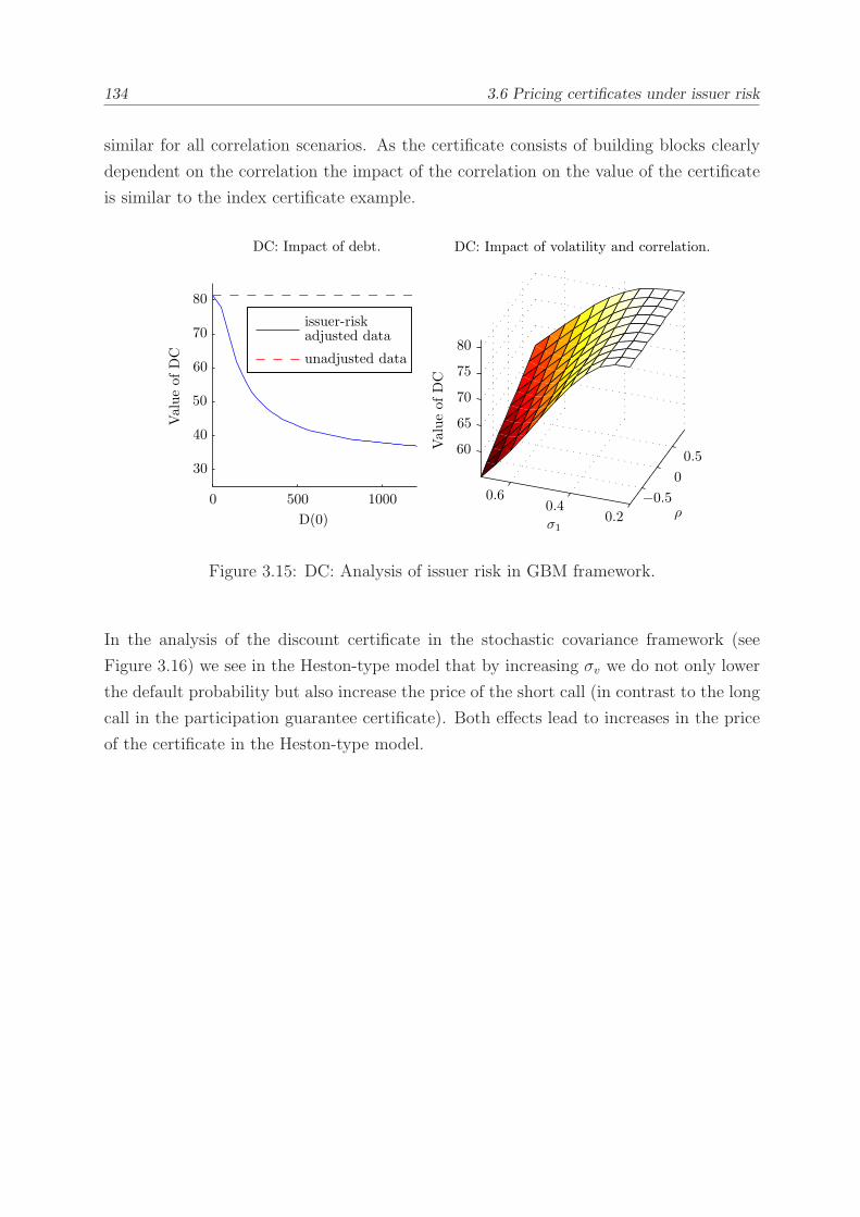
134 3.6 Pricing certificates under issuer risk
similar for all correlation scenarios. As the certificate consists of building blocks clearly
dependent on the correlation the impact of the correlation on the value of the certificate
is similar to the index certificate example.
DC: Impact of volatility and correlation.
Valueof
DC
σ1
ρ
unadjusted data
issuer-riskadjusted data
DC: Impact of debt.
Valueof
DC
D(0)
−0.50
0.5
0 500 10000.2
0.40.6
30
40
50
60
70
80
60
65
70
75
80
Figure 3.15: DC: Analysis of issuer risk in GBM framework.
In the analysis of the discount certificate in the stochastic covariance framework (see
Figure 3.16) we see in the Heston-type model that by increasing σv we do not only lower
the default probability but also increase the price of the short call (in contrast to the long
call in the participation guarantee certificate). Both effects lead to increases in the price
of the certificate in the Heston-type model.
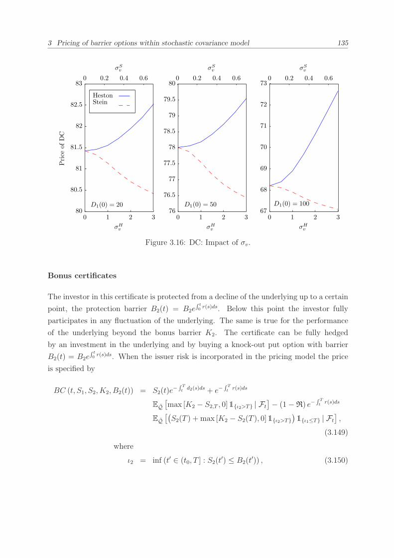
3 Pricing of barrier options within stochastic covariance model 135
σSv σS
vσSv
σHvσH
v
Price
ofDC
σHv
HestonStein
D1(0) = 20 D1(0) = 50 D1(0) = 100
0 0.2 0.4 0.6 0 0.2 0.4 0.60 0.2 0.4 0.6
0 1 2 30 1 2 30 1 2 367
68
69
70
71
72
73
76
76.5
77
77.5
78
78.5
79
79.5
80
80
80.5
81
81.5
82
82.5
83
Figure 3.16: DC: Impact of σv.
Bonus certificates
The investor in this certificate is protected from a decline of the underlying up to a certain
point, the protection barrier B2(t) = B2e∫ t0 r(s)ds. Below this point the investor fully
participates in any fluctuation of the underlying. The same is true for the performance
of the underlying beyond the bonus barrier K2. The certificate can be fully hedged
by an investment in the underlying and by buying a knock-out put option with barrier
B2(t) = B2e∫ t0 r(s)ds. When the issuer risk is incorporated in the pricing model the price
is specified by
BC (t, S1, S2, K2, B2(t)) = S2(t)e−∫ Tt
d2(s)ds + e−∫ Tt
r(s)ds
EQ[max [K2 − S2,T , 0]1ι2>T | Ft
]− (1−R) e−
∫ Tt
r(s)ds
EQ[(S2(T ) + max [K2 − S2(T ), 0]1ι2>T
)1ι1≤T | Ft
],
(3.149)
where
ι2 = inf (t′ ∈ (t0, T ] : S2(t′) ≤ B2(t
′)) , (3.150)
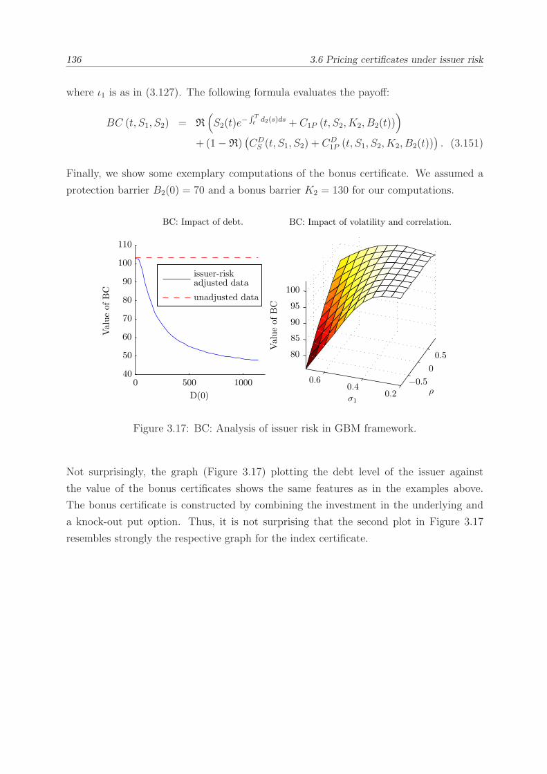
136 3.6 Pricing certificates under issuer risk
where ι1 is as in (3.127). The following formula evaluates the payoff:
BC (t, S1, S2) = R(
S2(t)e−∫ Tt
d2(s)ds + C1P (t, S2, K2, B2(t)))
+(1−R)(CD
S (t, S1, S2) + CD1P (t, S1, S2, K2, B2(t))
). (3.151)
Finally, we show some exemplary computations of the bonus certificate. We assumed a
protection barrier B2(0) = 70 and a bonus barrier K2 = 130 for our computations.
BC: Impact of volatility and correlation.
Valueof
BC
σ1
ρ
unadjusted data
issuer-riskadjusted data
BC: Impact of debt.
Valueof
BC
D(0)
−0.50
0.5
0 500 10000.2
0.40.6
40
50
60
70
80
90
100
110
80
85
90
95
100
Figure 3.17: BC: Analysis of issuer risk in GBM framework.
Not surprisingly, the graph (Figure 3.17) plotting the debt level of the issuer against
the value of the bonus certificates shows the same features as in the examples above.
The bonus certificate is constructed by combining the investment in the underlying and
a knock-out put option. Thus, it is not surprising that the second plot in Figure 3.17
resembles strongly the respective graph for the index certificate.
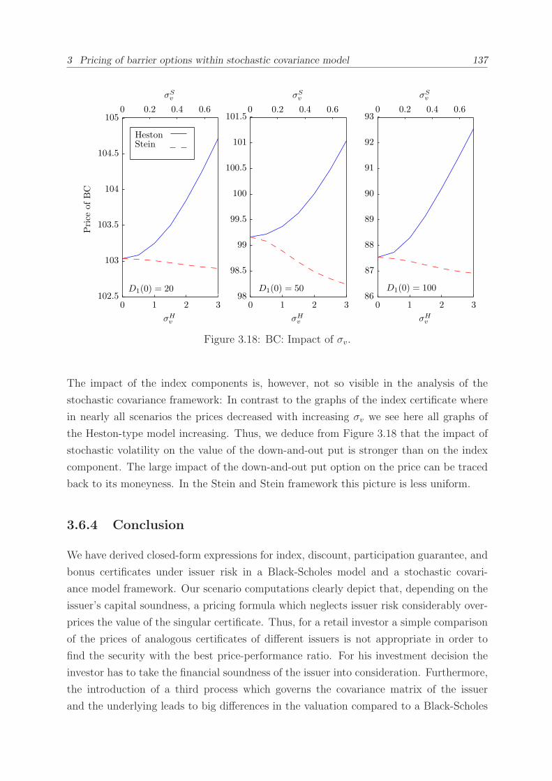
3 Pricing of barrier options within stochastic covariance model 137
σSvσS
v σSv
σHvσH
v
Price
ofBC
σHv
HestonStein
D1(0) = 20 D1(0) = 50 D1(0) = 100
0 0.2 0.4 0.60 0.2 0.4 0.6 0 0.2 0.4 0.6
0 1 2 30 1 2 30 1 2 386
87
88
89
90
91
92
93
98
98.5
99
99.5
100
100.5
101
101.5
102.5
103
103.5
104
104.5
105
Figure 3.18: BC: Impact of σv.
The impact of the index components is, however, not so visible in the analysis of the
stochastic covariance framework: In contrast to the graphs of the index certificate where
in nearly all scenarios the prices decreased with increasing σv we see here all graphs of
the Heston-type model increasing. Thus, we deduce from Figure 3.18 that the impact of
stochastic volatility on the value of the down-and-out put is stronger than on the index
component. The large impact of the down-and-out put option on the price can be traced
back to its moneyness. In the Stein and Stein framework this picture is less uniform.
3.6.4 Conclusion
We have derived closed-form expressions for index, discount, participation guarantee, and
bonus certificates under issuer risk in a Black-Scholes model and a stochastic covari-
ance model framework. Our scenario computations clearly depict that, depending on the
issuer’s capital soundness, a pricing formula which neglects issuer risk considerably over-
prices the value of the singular certificate. Thus, for a retail investor a simple comparison
of the prices of analogous certificates of different issuers is not appropriate in order to
find the security with the best price-performance ratio. For his investment decision the
investor has to take the financial soundness of the issuer into consideration. Furthermore,
the introduction of a third process which governs the covariance matrix of the issuer
and the underlying leads to big differences in the valuation compared to a Black-Scholes

138 3.6 Pricing certificates under issuer risk
framework. We have analysed the behaviour of the certificate prices for rising stochas-
ticity in the covariance in detail. The choice of the assumed stochastic covariance model
considerable influences the price dynamics, e.g. the price in the Heston-type model reacts
completely different to a rise in the volatility of the covariance process than the value in
the Stein-type model.
Chapter 4
Pricing of barrier options within
stochastic correlation model
4.1 Introduction
As already mentioned, local and stochastic volatility models have been in place for some
years now, e.g. Dupire [37] or Stein and Stein [111] and Heston [65]. A natural extension
of the latter ones is a multivariate model with stochastic correlation, not only stochastic
covariance like the model presented in Section 3. And indeed, the performance of a
portfolio or a multi-dimensional derivative depends very much on the joint behaviour of the
underlyings, i.e. the covariances. Correlations are not constant over time. The popularity
of discrete stochastic correlation models like the Dynamic Conditional Correlation (DCC)
model proposed by Engle [40] supports this idea. Stylised facts featured by historical
data as well as by implicit market prices, e.g. the smile and skew of volatilities and
correlations, can be captured by the assumption of a stochastic behaviour of correlation
(besides volatility) (see e.g. da Fonseca et al. [26], Christoffersen et al. [23]). There are
two main problems with the modelling of correlation: One is the model to choose to keep
the correlation between −1 and 1 and the other is intractability because the number of
parameters grows exponentially when the dimensions are increased.
Gourieroux et al. [58], Philipov and Glickman [92] and da Fonseca et al. [27], [26] pro-
pose the use of Wishart processes to model stochastic multivariate covariance matrices.
However, this approach is rather cumbersome when it comes to estimation and simu-
lation. Pigorsch and Stelzer [93] and Muhle-Karbe et al. [89] present a multivariate
stochastic volatility model of OU-Wishart type, which is analytically tractable, however
the dimensions increase which renders a calibration rather complicated.

140 4.1 Introduction
In their discrete modelling works Kim et al. [77], Aguilar and West [2], Pitt and Shephard
[94] Chib et al. [22] suggest a multivariate factor stochastic volatility model to represent
stochastic dependencies between the underlyings. The factor models as well as our prin-
cipal component model reduce the dimension of the original problem. Our paper is based
on a stochastic principal component model introduced earlier by works of Escobar et al.
[42] and Escobar et al. [41]. This framework introduces stochastic eigenvalues and, thus,
avoids proliferation of parameters as the number of eigenvalues can be diminished to a
suitable number. Other publications applying principal component analysis are in support
of the fact that two to three eigenvalues are sufficient to describe most of the variation in
the portfolio (see Alexander [3], [4]).
Moreover, our model easily extends the Heston model to more underlyings: We allow
for stochastic volatility and at the same time for stochastic correlation among assets
and between variance and assets as well as between assets and correlation. The basic
stochastic principal component model is an affine model for which the characteristic func-
tion is available and allows for easy calibration to plain vanilla instruments. Even some
parametrisations of the extension to the stochastic principal component model which is
presented here feature an affine characteristic function.
We continue in this chapter to price barrier derivatives in one and two dimensions as in
Chapter 3 but now within the context of the principal component model. By means of
the affine characteristic function in some parametrisations of the model we are able to
find analytical expressions for single-barrier options. However, as mentioned in Chapter
3 we are not able to find a closed-form solution for two barriers in two dimensions and we
hence follow a perturbation theory approximation. The accuracy of the approximation is
analytically proven.
Hence, in this line of development, our work improves previous literature on correlation
risk and default dependencies: The here presented model assumes stochastic correlation
between the assets, and the pricing stays feasible. The simplicity of the approximative
pricing scheme is a key element of a good pricing performance.
This chapter is structured as follows. In Section 4.2 we give a short insight in the stochastic
principal component model and we empirically motivate the structure of the model (see
Section 4.3). We derive closed-form solutions for single-asset instruments such as single-
barrier call options in this framework in Section 4.4. To solve for barrier options on two
underlyings we apply an approximation, which is motivated by perturbation theory in
Section 4.5.
4 Pricing of barrier options within stochastic correlation model 141
4.2 Model framework
The system of processes is defined on a filtered probability space (Ω,F , Q,F) where F0
contains all subsets of the (Q−) null sets of F and F is right-continuous. We define the
processes under the risk-neutral measure Q.
We introduce a fast mean-reverting stochastic principal component model. In the next
section we motivate the choice of a fast mean-reverting component to the eigenvalue
empirically. One can think of the fast mean-reverting component as influenced by the
fast mean reversion of the volatility which has been found by several authors (see [125],
[46]). In our analysis we limit ourselves for demonstration purposes to two underlyings.
However, an extension to d underlyings is straight forward.
dSi = rSidt+ Si
p∑
j=1
aijf(vj(t))dWj, i ∈ 1, 2 , p = 2, (4.1)
dvj =κvjδ2j
(ζvj − vj)dt+σvjδj
√vjdZj, (4.2)
〈dWi, dZj〉 = 0,
〈dWj, dZj〉 = ρvjdt,
〈dWi, dWj〉 = 0, for j ∈ 1, 2 .
f(vj) represents the jth eigenvalue of the instantaneous covariance matrix Σ of the under-
lying process Si. The eigenvalues are driven by a fast mean-reverting Cox-Ingersoll-Ross
process with mean-reversion rateκj
δj, where we assume δj very small. We further suppose
that the eigenvalues f(vj) are positive and bounded. We assume that there are constants
o11, o12, o21, o22 such that 0 < oj1 ≤ f(vj) ≤ oj2, for all j ≤ p. (aij) represents the (2× 2)
matrix of eigenvectors. For any fixed time t the process decomposes into two orthogonal
directions given by the eigenvectors aij, which are not dependent on time. We presume
that the Feller condition is satisfied for all processes.
In the following we denote the instantaneous variance of the log-asset lnSi by σ2Si
and the
instantaneous correlation between the two assets lnSi and lnSk by ρSi,Sk.
Remark 15. The log-assets exhibit stochastic variance and correlation given by
σ2Si(t) =
2∑
j=1
a2ijf (vj(t))2 ,
ρSi,Sk(t) =
∑2j=1 aijakjf (vj(t))
2
√∑2
j=1 a2ijf (vj(t))
2√∑p
j=1 a2kjf (vj(t))
2. (4.3)
142 4.2 Model framework
Proof.
The expression(4.3) can be obtained by applying Ito’s formula (see Theorem 18) and
quadratic variation (see Definition 36). Thus, with
df (vj(t))2 =
(
∂f (vj(t))2
∂vj
κvjδ2j
(ζvj − vj
)+
1
2
∂2f (vj(t))2
∂v2j
σ2vj
δ2jvj
)
dt
+∂f (vj(t))
2
∂vj
σvjδj
√vjdZvj (4.4)
and
σ2f(vj(t))
=
(
∂f (vj(t))2
∂vj
)2σ2vj
δ2jvj, (4.5)
the results follow.
Theorem 39. (Characteristic function)
For any time t the joint conditional characteristic function ϕ(t′ − t,u) =
E [exp i 〈ux(t′)〉 |Ft ] of the log-assets x1 = ln(
S1e∫ t′
tr(s)ds
)
and x2 = ln(
S2e∫ t′
tr(s)ds
)
,
where S1 and S2 are given by Model (4.1), satisfies the following PDE
− ∂ϕ (τ,u)
∂τ+
2∑
i=1
(
r − 1
2
2∑
j=1
a2ijf (vj(t))2
)
∂ϕ (τ,u)
∂xi
+1
2
2∑
i,k=1
∂2ϕ (τ,u)
∂xi∂xk
2∑
j=1
aijakjf (vj(t))2
+2∑
j=1
(κvjδ2j
(ζvj − vj
) ∂ϕ (τ,u)
∂vj+
1
2
σ2vj
δ2jvj∂2ϕ (τ,u)
∂v2j
)
+2∑
i=1
2∑
j=1
aijf (vj(t))
(
ρvj√vjσvjδj
∂2ϕ (τ,u)
∂xi∂vj
)
= 0, (4.6)
where τ = t′ − t, t′ > t, with initial condition ϕ(0,u) = exp i 〈ux〉.
Proof. The theorem trivially follows from Ito’s Lemma.
4 Pricing of barrier options within stochastic correlation model 143
Corollary 16. (Special case)
In the case ρvj = 0, ∀j, and f (vj) = √vj the characteristic function has an affine solution
given by
ϕ (τ,u) = exp
i 〈ux〉+ A∗H (τ,u) +
2∑
j=1
δ2jσ2vj
B∗H1j (τ,u) vj
,
(4.7)
where
B∗H1j (τ,u) =
κvjδ2j− dvj
sinh(
dvj2τ)
+κvj
δ2j dvjcosh
(dvj2τ)
cosh(
dvj2τ)
+κvj
δ2j dvjsinh
(dvj2τ) , (4.8)
A∗H (τ,u) = τ
(
ir (u1 + u2) +2∑
j=1
κ2vjδ2jσ
2vj
ζvj
)
−22∑
j=1
(κvjσ2vj
ζvj ln
(κvjδ2jdvj
sinh
(dvj
2τ
)
+ cosh
(dvj
2τ
)))
, (4.9)
dvj = dvj(u) =
√
κ2vjδ4j
+σ2vj
δ2j
(i(u1a21j + u2a22j
)+ 2u1u2a1ja2j + u21a
21j + u22a
22j
).
This characteristic function is well defined and analytic in a neighbourhood of 0.
For a proof refer to Appendix B.1.
4.3 Data analysis for mean-reversion scales
In the following1 we study if there exists a fast mean-reversion scale of the eigenvalues
and/or covariances of the assets as suggested by the model. In our analysis we follow the
lines of Fouque et al. [51], who analyse variograms of the log absolute returns for the
mean-reversion speed, and extend their approach to two dimensions from an underlying
perspective. As proposed by our model we assume constant orthonormal eigenvectors
(a11, a21)′ and (a12, a22)
′ and focus on the estimation of the mean-reversion speed param-
eters κ∗vj =κvj
δ2j, j = 1, 2, of the dynamics of the eigenvalues f(v1) := f1 and f(v2) := f2.
In order to facilitate the estimation we set the correlation between the Brownian motions
1The following chapter has been prepared in cooperation with Daniela Neykova during her master thesisproject. See [90].
144 4.3 Data analysis for mean-reversion scales
for the assets and the volatility processes ρvj , j = 1, 2, to zero. An analysis by Fouque et
al. (see [49], p. 81ff) showed in a one-dimensional setting that the rate of mean-reversion
was insensitive to the correlation parameter.
Our data set2 comprises stock prices of the three companies IBM, Apple and Dell. We
use their high-frequency intra-day data over one year (from October 1, 2008 to September
30, 2009) to proof our hypothesis of the existence of a fast mean-reverting factor. To es-
timate the covariance matrices3 we apply daily stock-price data over 15 years (from June
30, 1995 to June 30, 2010). The large data set should ensure the stability of the estima-
tors. The high-frequency data points are averaged over intervals of 5 minutes. Intervals
during working days without any observations are collapsed. So we finally end up with
78 matching observations per company per day, thus a total of 19, 593 data points per
company. Furthermore, the high-frequency data must be adjusted by the day effect, i.e.
the systematic effect that the volatility is the highest at the beginning of the day when
trading starts and at the end of the day. We follow here Fouque et al. [51] who model
the day effect by fitting a periodical function to the 78 observations.
The steps which are described in the following are performed for both time series, the
daily and the intra-day data, separately for a combination of two companies at a time.
We adjust the stock price returns by their means and normalise the data:
Sd1(n) :=
2(S1(n)− S1(n− 1))√∆t(S1(n) + S1(n− 1))
,
Sd2(n) :=
2(S2(n)− S2(n− 1))√∆t(S2(n) + S2(n− 1))
, n = 1, 2, . . . , (4.10)
where n describes the nth observation, ∆t is either 5 minutes in the case of the high-
frequency data or 1 day in the case of the daily data, and Si denotes the mean-adjusted
data point. When we theoretically discretise the stock price processes (4.1) by applying
Euler approximation4
∆S1(n)
S1(n)√∆t
= µ1
√∆t+ a11f1(v1(n))
∆W1(n)√∆t
+ a12f2(v2(n))∆W2(n)√
∆t,
∆S2(n)
S2(n)√∆t
= µ2
√∆t+ a21f1(v1(n))
∆W1(n)√∆t
+ a22f2(v2(n))∆W2(n)√
∆t, (4.11)
n = 1, 2, . . .
where (ai1, ai2)′ describe the eigenvalues of asset Si, f(vj(n)) := fj(n) is the positive
2The data has been downloaded from The Trade and Quote (TAQ) database.3Note that we assume constant eigenvectors.4Note that we work now under the pricing measure. µi are r in the risk-neutral world (see (4.1)).
4 Pricing of barrier options within stochastic correlation model 145
eigenfunction process, and ∆Wj is the respective increment of the Brownian motion Wj,
we see that
Sd1(n) = a11f1(n)
∆W1(n)√∆t
+ a12f2(n)∆W2(n)√
∆t,
Sd2(n) = a21f1(n)
∆W1(n)√∆t
+ a22f2(n)∆W2(n)√
∆t, n = 1, 2, . . . . (4.12)
To extract the behaviour of f1 and f2 from the data we de-correlate the two-dimensional
discrete process (Sd1 , S
d2)
′ by multiplying it with the eigenvectors of the covariance matrix
for (ln(S1), ln(S2))′. As already mentioned our assumptions of constant eigenvectors allows
us to estimate the covariance matrix from the daily data set over its whole period from
1995 to 2010. From there we gain the two eigenvectors
(
a11
a21
)
and
(
a12
a22
)
.
(
Sd1(n)
Sd2(n)
)
=
(
a11 a21
a12 a22
)(
Sd1(n)
Sd2(n)
)
, n = 1, 2, . . . . (4.13)
We, thus, obtain the two independent time series (Sd1 , S
d2)
′ for our high-frequency data.
Sd1(n) = f1(n)
∆W1(n)√∆t
and Sd2(n) = f2(n)
∆W2(n)√∆t
, n = 1, 2, . . . . (4.14)
As mentioned above the day effect in the intra-day data, i.e. the fact that the volatility of
stocks is especially high when the stock exchanges open and decreases to a lower level in
the course of time over the day before it rises again, has to be accounted for. We include
this effect into our model by replacing (4.14) with
Sd1(n) = f1(n)f
d1 (n)
∆W1(n)√∆t
and Sd2(n) = f2(n)f
d2 (n)
∆W2(n)√∆t
, n = 1, 2, . . . , (4.15)
where fdj (n), j = 1, 2 is a periodic function of day-time with period 78 (which corresponds
to the 78 observation points per day). For the estimation of the periodic function we treat
each data point Sd1(n) as influenced by the realisation of the function fd
j (n) at the time
point n, n = 1, . . . , 78. We compute the root-mean square over all data points Sd1(n)
realised at a certain time n, n = 1, . . . , 78, e.g. for the calculation of the first root mean-
square at n = 1 we take all those data points into account which were realised at 9am.
The result of all 78 root-mean squares is presented in Figure 4.1 for the examples Dell
and Apple. The graph falls until a certain point in time before it increases again. This
form could be reversed engineered with the sum of two exponential functions, one with
a component exp
−n/l(j)1
, which causes a decrease in n, and one with a component
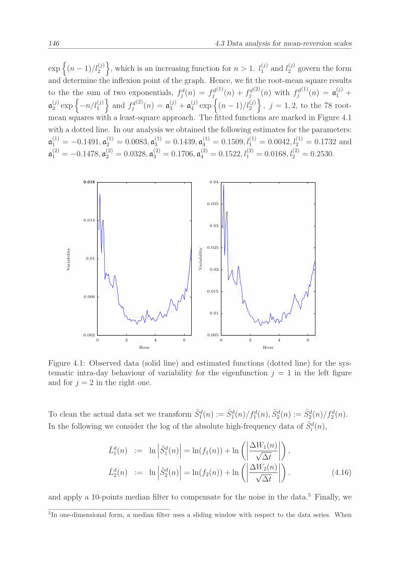
146 4.3 Data analysis for mean-reversion scales
exp
(n− 1)/l(j)2
, which is an increasing function for n > 1. l(j)1 and l
(j)2 govern the form
and determine the inflexion point of the graph. Hence, we fit the root-mean square results
to the the sum of two exponentials, fdj (n) = fd
j
(1)(n) + fd
j
(2)(n) with fd
j
(1)(n) = a
(j)1 +
a(j)2 exp
−n/l(j)1
and fdj
(2)(n) = a
(j)3 + a
(j)4 exp
(n− 1)/l(j)2
, j = 1, 2, to the 78 root-
mean squares with a least-square approach. The fitted functions are marked in Figure 4.1
with a dotted line. In our analysis we obtained the following estimates for the parameters:
a(1)1 = −0.1491, a(1)2 = 0.0083, a
(1)3 = 0.1439, a
(1)4 = 0.1509, l
(1)1 = 0.0042, l
(1)2 = 0.1732 and
a(2)1 = −0.1478, a(2)2 = 0.0328, a
(2)3 = 0.1706, a
(2)4 = 0.1522, l
(2)1 = 0.0168, l
(2)2 = 0.2530.
Variability
Hour
Variability
Hour
0 2 4 60 2 4 6
0.005
0.01
0.015
0.02
0.025
0.03
0.035
0.04
0.002
0.006
0.01
0.014
0.0180.018
Figure 4.1: Observed data (solid line) and estimated functions (dotted line) for the sys-tematic intra-day behaviour of variability for the eigenfunction j = 1 in the left figureand for j = 2 in the right one.
To clean the actual data set we transform Sd1(n) := Sd
1(n)/fd1 (n), S
d2(n) := Sd
2(n)/fd2 (n).
In the following we consider the log of the absolute high-frequency data of Sdi (n),
Ld1(n) := ln
∣∣∣Sd
1(n)∣∣∣ = ln(f1(n)) + ln
(∣∣∣∣
∆W1(n)√∆t
∣∣∣∣
)
,
Ld2(n) := ln
∣∣∣Sd
2(n)∣∣∣ = ln(f2(n)) + ln
(∣∣∣∣
∆W2(n)√∆t
∣∣∣∣
)
. (4.16)
and apply a 10-points median filter to compensate for the noise in the data.5 Finally, we
5In one-dimensional form, a median filter uses a sliding window with respect to the data series. When
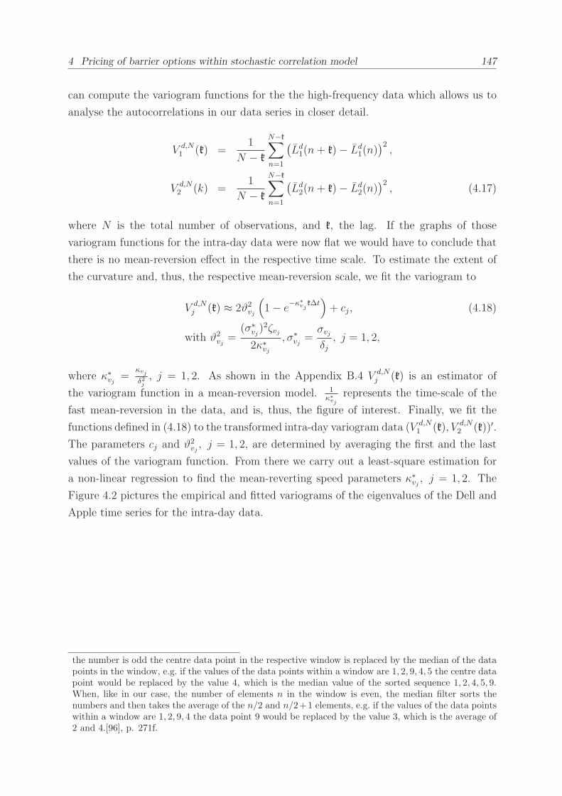
4 Pricing of barrier options within stochastic correlation model 147
can compute the variogram functions for the the high-frequency data which allows us to
analyse the autocorrelations in our data series in closer detail.
V d,N1 (k) =
1
N − k
N−k∑
n=1
(Ld1(n+ k)− Ld
1(n))2,
V d,N2 (k) =
1
N − k
N−k∑
n=1
(Ld2(n+ k)− Ld
2(n))2, (4.17)
where N is the total number of observations, and k, the lag. If the graphs of those
variogram functions for the intra-day data were now flat we would have to conclude that
there is no mean-reversion effect in the respective time scale. To estimate the extent of
the curvature and, thus, the respective mean-reversion scale, we fit the variogram to
V d,Nj (k) ≈ 2ϑ2
vj
(
1− e−κ∗vj
k∆t)
+ cj, (4.18)
with ϑ2vj=
(σ∗vj)2ζvj
2κ∗vj, σ∗
vj=σvjδj, j = 1, 2,
where κ∗vj =κvj
δ2j, j = 1, 2. As shown in the Appendix B.4 V d,N
j (k) is an estimator of
the variogram function in a mean-reversion model. 1κ∗vj
represents the time-scale of the
fast mean-reversion in the data, and is, thus, the figure of interest. Finally, we fit the
functions defined in (4.18) to the transformed intra-day variogram data (V d,N1 (k), V d,N
2 (k))′.
The parameters cj and ϑ2vj, j = 1, 2, are determined by averaging the first and the last
values of the variogram function. From there we carry out a least-square estimation for
a non-linear regression to find the mean-reverting speed parameters κ∗vj , j = 1, 2. The
Figure 4.2 pictures the empirical and fitted variograms of the eigenvalues of the Dell and
Apple time series for the intra-day data.
the number is odd the centre data point in the respective window is replaced by the median of the datapoints in the window, e.g. if the values of the data points within a window are 1, 2, 9, 4, 5 the centre datapoint would be replaced by the value 4, which is the median value of the sorted sequence 1, 2, 4, 5, 9.When, like in our case, the number of elements n in the window is even, the median filter sorts thenumbers and then takes the average of the n/2 and n/2+1 elements, e.g. if the values of the data pointswithin a window are 1, 2, 9, 4 the data point 9 would be replaced by the value 3, which is the average of2 and 4.[96], p. 271f.
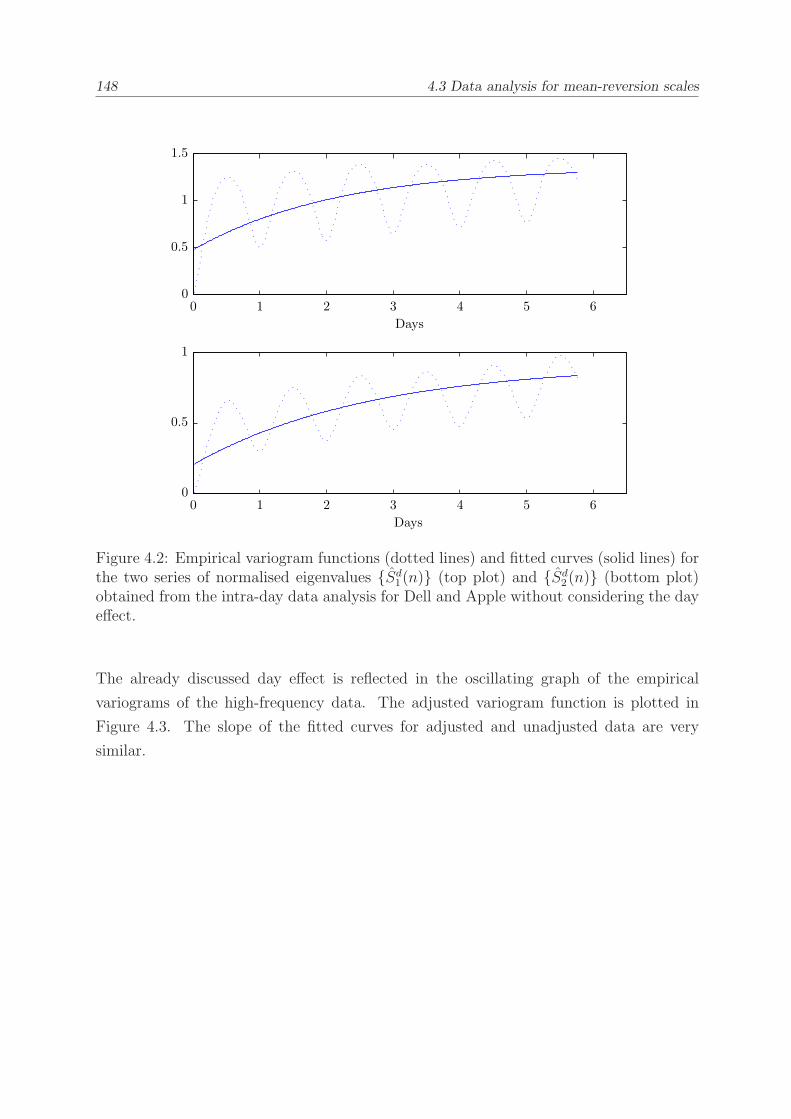
148 4.3 Data analysis for mean-reversion scalesreplacemen
Days
Days
0 1 2 3 4 5 6
0 1 2 3 4 5 6
0
0.5
1
0
0.5
1
1.5
Figure 4.2: Empirical variogram functions (dotted lines) and fitted curves (solid lines) forthe two series of normalised eigenvalues Sd
1(n) (top plot) and Sd2(n) (bottom plot)
obtained from the intra-day data analysis for Dell and Apple without considering the dayeffect.
The already discussed day effect is reflected in the oscillating graph of the empirical
variograms of the high-frequency data. The adjusted variogram function is plotted in
Figure 4.3. The slope of the fitted curves for adjusted and unadjusted data are very
similar.
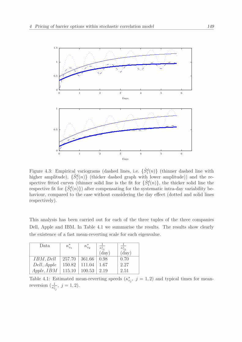
4 Pricing of barrier options within stochastic correlation model 149
Days
Days
0 1 2 3 4 5 6
0 1 2 3 4 5 6
0
0.5
1
0
0.5
1
1.5
Figure 4.3: Empirical variograms (dashed lines, i.e. Sd1(n) (thinner dashed line with
higher amplitude), Sd1(n) (thicker dashed graph with lower amplitude)) and the re-
spective fitted curves (thinner solid line is the fit for Sd1(n), the thicker solid line the
respective fit for Sd1(n)) after compensating for the systematic intra-day variability be-
haviour, compared to the case without considering the day effect (dotted and solid linesrespectively).
This analysis has been carried out for each of the three tuples of the three companies
Dell, Apple and IBM. In Table 4.1 we summarise the results. The results show clearly
the existence of a fast mean-reverting scale for each eigenvalue.
Data κ∗v1 κ∗v21
κ∗v1
(day)
1κ∗v2
(day)IBM,Dell 257.70 361.66 0.98 0.70Dell, Apple 150.82 111.04 1.67 2.27Apple, IBM 115.10 100.53 2.19 2.51
Table 4.1: Estimated mean-reverting speeds (κ∗vj , j = 1, 2) and typical times for mean-
reversion ( 1κ∗vj
, j = 1, 2).
150 4.4 Pricing of single-barrier options
4.4 Pricing of single-barrier options
The marginal knock-out barrier option has a payout g(S1), which may depend on S1(T ) at
maturity time T provided that S1(t) has not crossed a predefined time-dependent barrier
B1(t) = B1e∫ t0 r(s)ds prior to maturity. When we assume risk-neutral valuation the value
of a general barrier option with a time-dependent barrier on its underlying is given by
C(t, S1, B1,v) = EQ
[
e−∫ Tt
r(s)dsg (S1(T ))1ι1>T |Ft
]
,
where
ι1 = inf (t′ ∈ (t, T ] : S1(t′) ≤ B1(t
′)) , (4.19)
where the expectation is taken with respect to the pricing measure Q.g (S1(T )) describes the part of the payoff which depends on the value of S1 in T . The
following PDE can be derived for the Model (4.1) with ρvj = 0. The restriction is necessary
to apply the method of images.
∑2j=1
(12a21jf(vj)
2S21∂2C∂S2
1
)
+ rS1∂C∂S1
+ ∂C∂t− rC
+∑2
j=1
(κvj
δ2j(ζvj − vj) ∂C∂vj +
12
σ2vj
δ2jvj
∂2C∂v2j
)
= 0,
C (t, B1(t), B1(t),v) = 0, C (T, S1, B1(t),v) = g (S1)1ι1>T.
The PDE can be reduced to
∑2j=1
(12a21jf(vj)
2 ∂2G∂x2
1− 1
2a21jf(vj)
2 ∂G∂x1
)
+ ∂G∂t
+∑2
j=1
(κvj
δ2j(ζvj − vj) ∂G∂vj +
12
σ2vj
δ2jvj
∂2G∂v2j
)
= 0,
G (t, b1, b1,v) = 0, G (T, x1, b1,v) = g (x1)1ι1>T,
where we use the transformations x1(t) := ln
(
S1(t)e∫Tt r(s)ds
K1
)
, b1 := ln(
B1(T )K1
)
, and
G (t, x1, b1,v) := e∫ Tt
r(s)dsC (t, S1, B1,v). See also Appendix A.1.1. Following the lines
of the derivation in Section 3.4 we can then derive the following theorem on pricing a
single-barrier option.
Theorem 40. (Single-barrier option pricing in Model (4.1))
Let us assume
i. the setting described in Equation (4.1) as well as ρvj=0,
ii. the existence of an affine analytic characteristic function ϕ(τ, u1) in z1, which is
4 Pricing of barrier options within stochastic correlation model 151
regular in a neighbourhood Sϕ = u1 = w1 + iω1 : ω1 ∈ (aϕ, bϕ) , aϕ < 0, bϕ > 0 of
the origin, and integrable, and
iii. that the generalized Fourier transform h(x1) of the payoff function e−x12 g(x1) at
maturity exists in a space Sg = u1 = w1 + iω1 : ω1 ∈ (ag, bg), is integrable for
|x1| <∞.
If the space SC ≡ Sϕ ∩ Sg is not empty, then the barrier option value (4.19) is given by
CB (t, S1, B1,v) =e
x12−∫ Tt
r(s)ds
2π
∫ iω1+∞
iω1−∞h(u1)
(ϕ(τ, u1,−x1)− ϕ(τ, u1, x1 − 2b1)) du1,
u1 ∈ SC , (4.20)
where
ϕ(τ, u1, x1) = exp
iu1x1 + A∗(τ, u1) +2∑
j=1
(
δ2jσ2vj
B∗1j(τ, u1)vj
)
,
h(u1) =
∫ +∞
−∞e−
x′12 g(x′1)e
iu1x′1dx′1, u1 ∈ Sg,
x1 = lnS1e
∫ Tt
r(s)ds
K1
, b1 = lnB1(T )
K1
,
where ϕ(τ, u1, x1) satisfies the PDE 4.6. The price converges point-wise if the map S1 →CB(t, S1, B1,v) is continuous.
Proof.
By introducing the following transformations
G(t, x1, b1,v) := ex12 Z(t, x1, b1,v),
∂G
∂x1=
1
2G+ e
x12∂Z
∂x1,
∂2G
∂x21=
1
4G+ e
x12∂Z
∂x1+ e
x12∂2Z
∂x21,
we can reduce the PDE problem (4.20) to
∑2j=1
(12a21jf(vj)
2 ∂2Z∂x2
1+ ∂G
∂t− 1
8
∑2j=1 a
21jf(vj)
2Z)
+∑2
j=1
(κvj
δ2j(ζvj − vj) ∂Z
∂vj+ 1
2
σ2vj
δ2jvj
∂2Z∂v2j
)
= 0,
Z (t, b1, b1,v) = 0, Z (T, x1, b1,v) = e−x12 g(x1)1ι1>T.
152 4.4 Pricing of single-barrier options
As in Section 3.4.1 we can specify the Kolmogorov backward equation and boundary
conditions of the transition probability density function p(t′, x′1,v′, t, x1,v). Since the
payoff of the derivative does not depend on the volatility, we pursue with
q(τ, x1,v, x′1) =
∫ ∞
0
p(τ, x1′,v′, x1,v)dv
′. (4.21)
Here q solves the Kolmogorov Equation (see Definition 38) supplied with the initial and
boundary conditions
q(0, x1, b1,v) = δ(x1 − x′1),q(τ, b1, b1,v) = 0. (4.22)
In the following we apply the reflection principle (see [76], p. 79f) (the counterpart to
the method of images in a half space in two dimensions (see A.1.3)), i.e. we first derive a
solution GF in the whole plane and restrict it to the space (see (4.22)) it is defined for by
using symmetries.
Assume an affine solution can be found6:
GF (τ, x′1,v; x1) =1
2π
∫ iω1+∞
iω1−∞exp
iu1(x′1 − x1) + A∗(τ, u1)
+2∑
j=1
( δ2jσ2vj
B∗1j(τ, u1)vj
)
du1,
u1 = v1 + iω1 ∈ Sϕ, (4.23)
where Sϕ describes a space in a neighbourhood to the origin, parallel to the real axis, in
which the integrand is regular.
The solution for q, satisfying the boundary conditions, can be found by the approach
q = GF + GG by using the symmetry of GF in x1 (see [83]). Note that the point 2b1 − x1is symmetric to x1 in b1. Thus, we set GG(τ, x′1 − x1,v) = −GF (τ, x′1 − 2b1 + x1,v). In
x1 = b1, GG = −GF and the boundary condition is, thus, satisfied. The PDE is also
6e.g. with f(vj) =√vj with B∗
1j = B∗
H1j(τ, u1) and A∗ = A∗
H(τ, u) given in (4.8)-(4.9),
dvj= dvj
(u) =
√
κ2vj
δ4j+
σ2vj
δ2j
(
u21a
21j +
1
4a21j
)
,
4 Pricing of barrier options within stochastic correlation model 153
satisfied by GG. Hence, the solution is given by
q(τ, x′1,v, x1) = GF (τ, x′1 − x1,v)− GF (τ, x′1 + x1 − 2b1,v)
=1
2π
∫ iω1+∞
iω1−∞exp
A∗(τ, u1) +2∑
j=1
(
δ2jσ2vj
B∗1j(τ, u1)vj
)
(4.24)
(exp iu1(x′1 − x1) − exp iu1(x′1 + x1 − 2b1)) du1.
From risk-neutral pricing, then
CB (t, S1, B1,v) = ex12−∫ Tt
r(s)ds
∫ ∞
−∞
(
e−x′12 g(x′1)q(τ, x
′1,v, x1)
)
dx′1. (4.25)
We have required that the payoff function, its transform and the characteristic function
are Lebesgue integrable in a space SC . Hence, we can apply Fubini’s theorem and change
the integrals if there exists a space SC = Sϕ ∩ Sg. Then, the above expression can be
simplified. We denote the Fourier transform of the payoff by h(u1)
h(u1) =
∫ +∞
−∞e−
x′12 g(x′1)e
iu1x′1dx′1, u1 ∈ Sg.
Then,
CB (t, S1, B1,v) =e
x12−∫ Tt
r(s)ds
2π
∫ iω1+∞
iω1−∞h(u1)
(ϕ (τ, u1,−x1)− ϕ(τ, u1, x1 − 2b1) du1,
u1 ∈ SC = Sϕ ∩ Sg,
where
ϕ(τ, u1, x1) = exp
iu1x1 + A∗(τ, u1) +2∑
j=1
(
δ2jσ2vj
B∗1j(τ, u1)vj
)
. (4.26)
If S1 → CB (t, S1, B1,v) is continuous the above relationship converges point-wise with
Theorem 33.
Exemplarily, we price single-barrier call options with gCall(S1) = max(S1 − K1, 0), i.e.
gCall(x1) = K1 max(ex1 − 1, 0). Thus, we have to Fourier transform e−12x1gCall(x1).
e−12x1gCall does not belong to L1. The ordinary Fourier transform does not exist and

154 4.4 Pricing of single-barrier options
we apply the generalized Fourier transform:
hCall(u1) = K1
∫ ∞
0
(ex′12 − e−
x′12 )eiu1x
′1dx′1
= K1
(
− 1
iu1 +12
+1
iu1 − 12
)
. (4.27)
Note that we choose ℑ(u1) > 12, i.e. SgCall
=u1 = w1 + iω1 : ω1 >
12
. Then, the price
of the barrier call option can be specified with
C1Call (t, S1, B1,v) =e
x12−∫ Tt
r(s)ds
2π
∫ iω1+∞
iω1−∞hCall(u1)
(ϕ(τ, u1,−x1)− ϕ(τ, u1, x1 − 2b1)) du1,
u1 ∈ SCCall= Sϕ ∩ SgCall
. (4.28)
hCall has a simple singularity in ω1 = 12. We can, thus, again apply residue calculus and
move the contour of integration to the real axis (see Corollary 3). With (2.56) we derive
the residue of hCall:
ResCall = limu1→i 1
2
(
u1 − i1
2
)
K1
(1
i(u1 − i12)(iu1 − 12)
)
= K1(−i)(−1) = K1i. (4.29)
Then by Corollary 3 the option price also equals the integral along the real axis of u1 minus
2πi times the residue of the Call price at u1 = i12, i.e. 2K1π
∫∞−∞ δ(u1−i12)
(
ϕ(τ, u1,−x1)−
ϕ(τ, u1, x1 − 2b1)
)
du1. See also [82]. The pricing formula with integration on the real
axis is then given by
C1Call(t, S1, B1,v) = ex12−∫ Tt
r(s)dsK1
(
ϕ(τ, i1
2,−x1,v)
−ϕ(τ, i12, x1 − 2b1)
)
+e
x12−∫ Tt
r(s)ds
2π
∫ ∞
−∞hCall(u1)
(ϕ(τ, u1,−x1)− ϕ(τ, u1, x1 − 2b1) du1,
u1 real. (4.30)
4 Pricing of barrier options within stochastic correlation model 155
4.5 Pricing of two-asset barrier options with pertur-
bation theory
Options with barriers on more than one underlying cannot be priced in closed form but
have to be approximated. Due to the form of our model an approximation using pertur-
bation techniques seems to be the right choice. In finance this method has been applied
to option pricing under a stochastic volatility model by Fouque et al. (see e.g. [47], [49]).
They theoretically prove the convergence of their approach in [52]. The approximation is
correct to an order of O(
δ12
)
and it is valid everywhere except in a boundary layer near
expiry. This group applied the approach to various option types, e.g. exotic options in
[70], Asian options in [48], defaultable bonds in [53]. Their approach has been extended
to additionally allow a slow mean-reverting component [50] and to multi-dimensions [55].
Howison [66] applies perturbation theory to price vanilla options near expiry, options in
illiquid markets etc. Howison [66], Rasmussen [101] as well as Conlon and Sullivan [24]
extend the expansion and show the convergence.
We shortly introduce perturbation theory. The introduction to perturbation theory is
based on the explications of Zauderer [121], p. 572ff.
Consider a differential equation
L(C, ǫ) = 0, (4.31)
that depends on the small positive parameter ǫ and is given over a spatial region D. For a
parabolic or hyperbolic problem the boundary conditions are assigned on ∂D and initial
data are given in D at the time t = 0. The so-called reduced or unperturbed problem
associated with (4.31) results when we set ǫ = 0 in (4.31), i.e. L(C, 0) = 0. The given
problem is called regular if the reduced problem has a unique solution. If this is not the
case we have to deal with a so called singular perturbation problem. When we set ǫ = 0
in a singular problem we obtain an equation for which either the order or the type of the
differential equation has changed.
For regular perturbation problems, the solution C is expanded in the perturbation series
C =∞∑
n=0
Cnǫn. (4.32)
The difference between C and C0 is called a perturbation on the solution C0 of the reduced

156 4.5 Pricing of two-asset barrier options with perturbation theory
or unperturbed problem. Inserting the expansion into (4.31) yields
L(C, ǫ) = L( ∞∑
n=0
Cnǫn, ǫ
)
= 0. (4.33)
The assumption is taken that L(C, ǫ) can be expanded in a power series in C and ǫ. Thus,
(4.31) can be written as a series
L(C, ǫ) =∞∑
n=0
Ln(Cn, Cn−1, . . . , C1, C0)ǫn = 0, (4.34)
where Ln describe differential operators which may be linear or non-linear, and which act
on the functions C0, C1, . . . , Cn. To solve the problem we equate the coefficients of ǫn in
(4.34) to zero (i.e. equating like powers of ǫ) and get
Ln(Cn, Cn−1, . . . , C1, C0) = 0, n = 0, 1, . . . . (4.35)
The same is true for any initial and/or boundary conditions. Hence, we obtain a system
of equations which we can solve recursively.
In the following sections we exemplary price two-asset options with and without barriers
in the Model (4.1) with perturbation theory, describe the convergence analytically and
give some numerical examples. Furthermore, we present a possible extension to Model
(4.1) and indicate how perturbation theory could also be applied in this model.
4.5.1 Approximation of Model (4.1)
We will see that the PDE for the valuation in fast mean-reversion models is a singular
perturbation problem. We will show that the singular perturbation can be applied and
converges everywhere except in a boundary layer near expiry. We also provide some
numerical results which back the theoretical convergence results.
By means of the perturbation technique we want to price options which depend on two
underlyings with and without barriers on both of the underlyings in the Model (4.1).
The payoff in T is indicated by g(S1, S2) in the following. Exemplarily, we show the
computations of a two-asset option with and without barriers (see [62] for two-asset digital
options without barriers). In the case of the option without barriers the value can be
determined by
C (t, S1, S2) = EQ
[
max(S2 −K2, 0)1S1>K1
]
, (4.36)

4 Pricing of barrier options within stochastic correlation model 157
the value of the barrier option is given by
CB(t, S1, S2, B1, B2) = EQ
[
max(S2 −K2, 0)1S1>K11ι1>T,ι2>T
]
, (4.37)
where ι1 = inf(
t′ ∈ ( t, T ] : S1(t′) ≤ B1(t
′))
and ι2 = inf(
t′ ∈ ( t, T ] : S2(t′) ≤ B2(t
′))
.
B1(t) and B2(t) describe the barriers on S1 and S2 respectively. As we presume fast
mean reversion for all the eigenvalues, i.e. δj → 0, C(S1, S2) and CB(S1, S2, B1, B2) can
be asymptotically approximated (see [49]). We pursue the expansion for the two-asset
option C (t, S1, S2) and only provide the expressions for CB(t, S1, S2, B1, B2) explicitly
when there are clear differences in the solutions.
First, we expand the problem in δ1 (see (4.32)), after that in δ2.
Cδ =∞∑
n=0
Cδ2n δ
n1 , (4.38)
Cδ2n =
∞∑
k=0
Cn,kδk2 . (4.39)
The infinitesimal generator Lδ is given by
Lδ :=1
δ21L1
0 +1
δ22L2
0 +1
δ1L1
1 +1
δ2L2
1 + L2. (4.40)
Note that it is expressed in the form of a power series in δj. Thus, the problem to be
solved for the two-asset option becomes
LδCδ = 0,
Cδ (T, S1, S2) = g(S1, S2), (4.41)
and for the barrier option, respectively
LδCδB = 0,
CδB(t, B1(t), S2) = 0,
CδB(t, S1, B2(t)) = 0,
CδB (T, S1, S2) = g(S1, S2), (4.42)
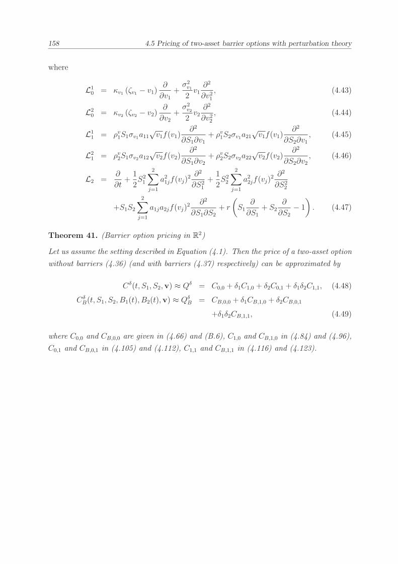
158 4.5 Pricing of two-asset barrier options with perturbation theory
where
L10 = κv1 (ζv1 − v1)
∂
∂v1+σ2v1
2v1∂2
∂v21, (4.43)
L20 = κv2 (ζv2 − v2)
∂
∂v2+σ2v2
2v2∂2
∂v22, (4.44)
L11 = ρv1S1σv1a11
√v1f(v1)
∂2
∂S1∂v1+ ρv1S2σv1a21
√v1f(v1)
∂2
∂S2∂v1, (4.45)
L21 = ρv2S1σv2a12
√v2f(v2)
∂2
∂S1∂v2+ ρv2S2σv2a22
√v2f(v2)
∂2
∂S2∂v2, (4.46)
L2 =∂
∂t+
1
2S21
2∑
j=1
a21jf(vj)2 ∂
2
∂S21
+1
2S22
2∑
j=1
a22jf(vj)2 ∂
2
∂S22
+S1S2
2∑
j=1
a1ja2jf(vj)2 ∂2
∂S1∂S2
+ r
(
S1∂
∂S1
+ S2∂
∂S2
− 1
)
. (4.47)
Theorem 41. (Barrier option pricing in R2)
Let us assume the setting described in Equation (4.1). Then the price of a two-asset option
without barriers (4.36) (and with barriers (4.37) respectively) can be approximated by
Cδ(t, S1, S2,v) ≈ Qδ = C0,0 + δ1C1,0 + δ2C0,1 + δ1δ2C1,1, (4.48)
CδB(t, S1, S2, B1(t), B2(t),v) ≈ Qδ
B = CB,0,0 + δ1CB,1,0 + δ2CB,0,1
+δ1δ2CB,1,1, (4.49)
where C0,0 and CB,0,0 are given in (4.66) and (B.6), C1,0 and CB,1,0 in (4.84) and (4.96),
C0,1 and CB,0,1 in (4.105) and (4.112), C1,1 and CB,1,1 in (4.116) and (4.123).
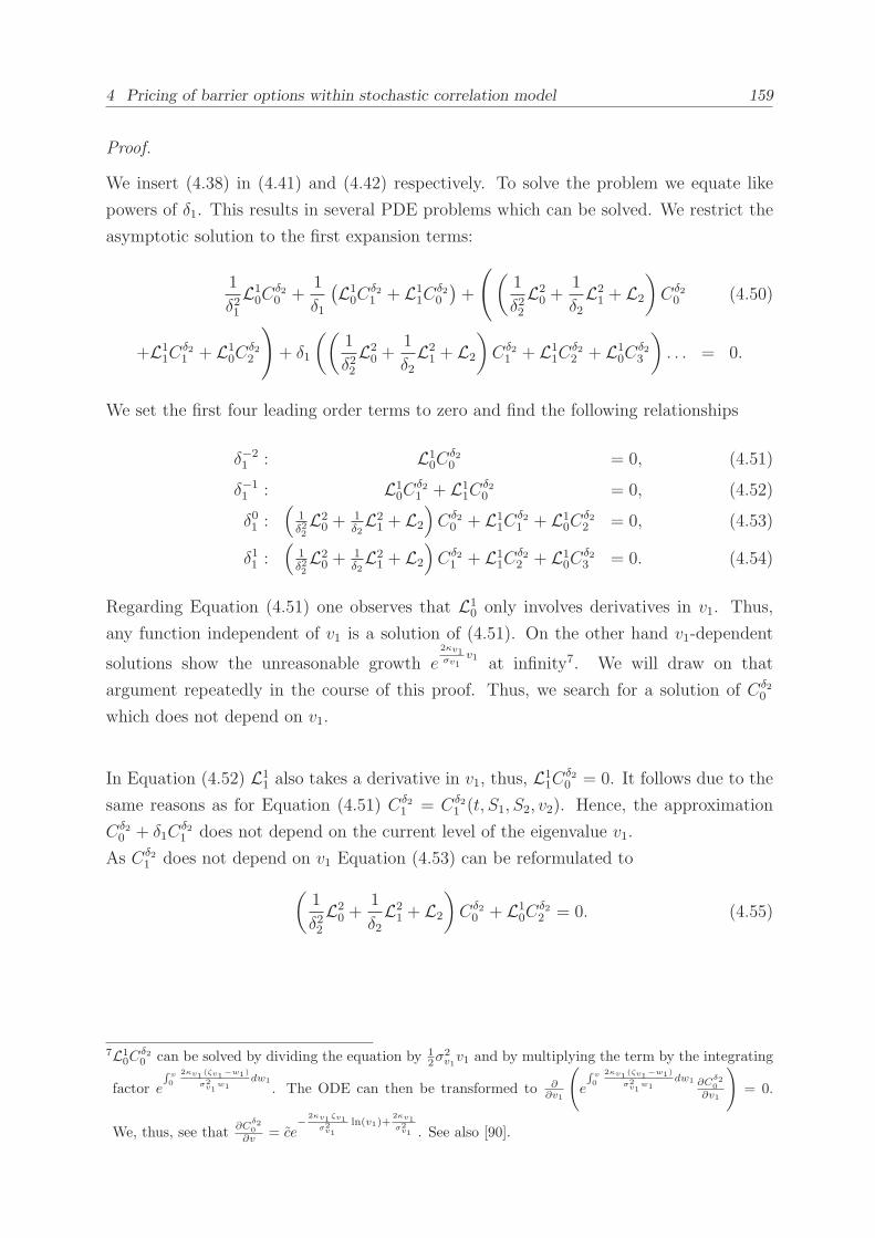
4 Pricing of barrier options within stochastic correlation model 159
Proof.
We insert (4.38) in (4.41) and (4.42) respectively. To solve the problem we equate like
powers of δ1. This results in several PDE problems which can be solved. We restrict the
asymptotic solution to the first expansion terms:
1
δ21L1
0Cδ20 +
1
δ1
(L1
0Cδ21 + L1
1Cδ20
)+
((1
δ22L2
0 +1
δ2L2
1 + L2
)
Cδ20 (4.50)
+L11C
δ21 + L1
0Cδ22
)
+ δ1
((1
δ22L2
0 +1
δ2L2
1 + L2
)
Cδ21 + L1
1Cδ22 + L1
0Cδ23
)
. . . = 0.
We set the first four leading order terms to zero and find the following relationships
δ−21 : L1
0Cδ20 = 0, (4.51)
δ−11 : L1
0Cδ21 + L1
1Cδ20 = 0, (4.52)
δ01 :(
1δ22L2
0 +1δ2L2
1 + L2
)
Cδ20 + L1
1Cδ21 + L1
0Cδ22 = 0, (4.53)
δ11 :(
1δ22L2
0 +1δ2L2
1 + L2
)
Cδ21 + L1
1Cδ22 + L1
0Cδ23 = 0. (4.54)
Regarding Equation (4.51) one observes that L10 only involves derivatives in v1. Thus,
any function independent of v1 is a solution of (4.51). On the other hand v1-dependent
solutions show the unreasonable growth e2κv1σv1
v1at infinity7. We will draw on that
argument repeatedly in the course of this proof. Thus, we search for a solution of Cδ20
which does not depend on v1.
In Equation (4.52) L11 also takes a derivative in v1, thus, L1
1Cδ20 = 0. It follows due to the
same reasons as for Equation (4.51) Cδ21 = Cδ2
1 (t, S1, S2, v2). Hence, the approximation
Cδ20 + δ1C
δ21 does not depend on the current level of the eigenvalue v1.
As Cδ21 does not depend on v1 Equation (4.53) can be reformulated to
(1
δ22L2
0 +1
δ2L2
1 + L2
)
Cδ20 + L1
0Cδ22 = 0. (4.55)
7L10C
δ20 can be solved by dividing the equation by 1
2σ2v1v1 and by multiplying the term by the integrating
factor e
∫
v
0
2κv1(ζv1
−w1)
σ2v1
w1dw1
. The ODE can then be transformed to ∂∂v1
(
e
∫
v
0
2κv1(ζv1
−w1)
σ2v1
w1dw1 ∂C
δ20
∂v1
)
= 0.
We, thus, see that∂C
δ20
∂v= ce
−
2κv1ζv1
σ2v1
ln(v1)+2κv1σ2v1 . See also [90].
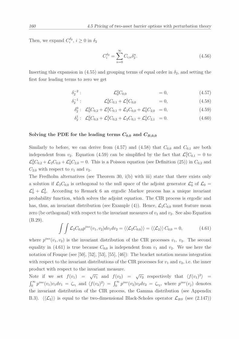
160 4.5 Pricing of two-asset barrier options with perturbation theory
Then, we expand Cδ2i , i ≥ 0 in δ2
Cδ2i =
∞∑
n=0
Ci,nδn2 . (4.56)
Inserting this expansion in (4.55) and grouping terms of equal order in δ2, and setting the
first four leading terms to zero we get
δ−22 : L2
0C0,0 = 0, (4.57)
δ−12 : L2
0C0,1 + L21C0,0 = 0, (4.58)
δ02 : L20C0,2 + L2
1C0,1 + L2C0,0 + L10C2,0 = 0, (4.59)
δ12 : L20C0,3 + L2
1C0,2 + L2C0,1 + L10C2,1 = 0. (4.60)
Solving the PDE for the leading terms C0,0 and CB,0,0
Similarly to before, we can derive from (4.57) and (4.58) that C0,0 and C0,1 are both
independent from v2. Equation (4.59) can be simplified by the fact that L21C0,1 = 0 to
L20C0,2 +L2C0,0 +L1
0C2,0 = 0. This is a Poisson equation (see Definition (25)) in C0,2 and
C2,0 with respect to v1 and v2.
The Fredholm alternatives (see Theorem 30, i(b) with iii) state that there exists only
a solution if L2C0,0 is orthogonal to the null space of the adjoint generator L∗0 of L0 =
L10 + L2
0. According to Remark 6 an ergodic Markov process has a unique invariant
probability function, which solves the adjoint equation. The CIR process is ergodic and
has, thus, an invariant distribution (see Example (4)). Hence, L2C0,0 must feature mean
zero (be orthogonal) with respect to the invariant measures of v1 and v2. See also Equation
(B.29). ∫ ∫
L2C0,0pinv(v1, v2)dv1dv2 = 〈〈L2C0,0〉〉 = 〈〈L2〉〉C0,0 = 0, (4.61)
where pinv(v1, v2) is the invariant distribution of the CIR processes v1, v2. The second
equality in (4.61) is true because C0,0 is independent from v1 and v2. We use here the
notation of Fouque (see [50], [52], [53], [55], [46]): The bracket notation means integration
with respect to the invariant distributions of the CIR processes for v1 and v2, i.e. the inner
product with respect to the invariant measure.
Note if we set f(v1) =√v1 and f(v2) =
√v2 respectively that 〈f(v1)2〉 =
∫∞0pinv(v1)v1dv1 = ζv1 and 〈f(v2)2〉 =
∫∞0pinv(v2)v2dv2 = ζv2 , where p
inv(vj) denotes
the invariant distribution of the CIR process, the Gamma distribution (see Appendix
B.3). 〈〈L2〉〉 is equal to the two-dimensional Black-Scholes operator LBS (see (2.147))

4 Pricing of barrier options within stochastic correlation model 161
with eigenvalues 〈f(v1)2〉 = f(v1)2 and 〈f(v2)2〉 = f(v2)2.
〈〈L2〉〉 = LBS
=∂
∂t+
1
2S21
2∑
j=1
a21j〈f(vj)2〉∂2
∂S21
+1
2S22
2∑
j=1
a22j〈f(vj)2〉∂2
∂S22
+S1S2
2∑
j=1
a1ja2j〈f(vj)2〉∂2
∂S1∂S2
+ r
(
S1∂
∂S1
+ S2∂
∂S2
− 1
)
. (4.62)
Hence, we can also write (4.61) as
LBS(σ1, σ2, ρ)C0,0 = 0, (4.63)
where the centred volatilities of S1 and S2, σ1 and σ2, and the centred correlation ρ
between the two assets can be indicated by
σ21 = a211〈f(v1)2〉+ a212〈f(v2)2〉,σ22 = a221〈f(v1)2〉+ a222〈f(v2)2〉,
ρ =a11a21〈f(v1)2〉+ a12a22〈f(v2)2〉
σ1σ2
. (4.64)
Corollary 17. (C0,0)
The term C0,0 is the solution of the following problem
LBS(σ1, σ2, ρ)C0,0 = 0,
C0,0 (T, S1, S2) = max(S2 −K2, 0)1S1>K1 . (4.65)
C0,0 can be evaluated by the following formula
C0,0 (t, S1, S2) = S2N2(d2,d1, ρ)−K2e−rτN2(d
∗2;d
∗1, ρ), (4.66)
where
τ = T − t, xi = lnSie
−∫ Tt
r(s)ds
Ki
,
d∗1 = d1 − ρσ2
√τ , d1 =
x1σ1
√τ− 1
2σ1
√τ + ρσ2
√τ ,
d∗2 = d2 − σ2
√τ , d2 =
x2σ2
√τ+
1
2σ2
√τ .
For a proof see Appendix B.2.

162 4.5 Pricing of two-asset barrier options with perturbation theory
Corollary 18. (CB,0,0)
CB,0,0, the respective expansion term for the two-asset option with two barriers, is given
by (see [62])
LBS(σ1, σ2, ρ)CB,0,0 = 0,
CB,0,0 (T, S1, S2) = max (S2 −K2, 0)1S1>K1 ,
CB,0,0(t, B1(t), S2) = 0,
CB,0,0(t, S1, B2(t)) = 0. (4.67)
(4.67) can be solved for ρ = − cos(2πkn
):
CB,0,0 (t, S1, S2, B1(t), B2(t)) =n−1∑
k=0
ey1
(
c1σ1−c1σ1 cos( 2πkn )+ 1√
1−ρ2(−c2σ2−ρc1σ1) sin( 2πk
n ))
(B2
(H+
1 −H−1
)− e−rτK2
(H+
2 −H−2
)), (4.68)
where
y1 =ln(
S1erτ
K1
)
− b1σ1
, y2 =ln(
S2erτ
K2
)
− b2σ2
,
c1 =σ1 − ρσ2
2σ1 (1− ρ2), c2 =
σ2 − ρσ1
2σ2 (1− ρ2)
H+1 = e
y2
(
c2σ2+(1−c2)σ2 cos( 2πkn )+ 1√
1−ρ2(c1σ1−ρ(1−c2)σ2) sin( 2πk
n ))
ey1
(
σ2√1−ρ2
sin( 2πkn )
)
N2
(l1(γ+1 , η
+2
), l2(γ+1 , η
+2
), ρ), (4.69)
H−1 = e
y2
(
c2σ2+(−(1−c2)σ2+2σ1c1ρ) cos( 2πkn )+ 1√
1−ρ2(−c1σ1(1−2ρ2)−ρ(1−c2)σ2) sin( 2πk
n ))
ey1
(
σ2√1−ρ2
sin( 2πkn )
)
N2
(l1(γ−1 , η
−2
), l2(γ−1 , η
−2
), ρ), (4.70)
H+2 = e
y2
(
c2σ2−c2σ2 cos( 2πkn )+ 1√
1−ρ2(c1σ1+ρc2σ2) sin( 2πk
n ))
N2
(l1(γ+1 , γ
+2
), l2(γ+1 , γ
+2
), ρ), (4.71)
H−2 = e
y2
(
c2σ2+(c2σ2+2σ1c1ρ) cos( 2πkn )+ 1√
1−ρ2(−c1σ1(1−2ρ2)+ρc2σ2) sin( 2πk
n ))
N2
(l1(γ−1 , γ
−2
), l2(γ−1 , γ
−2
), ρ),

4 Pricing of barrier options within stochastic correlation model 163
l1 (k1, k2) =√T − t (k1 + ρk2) +
b1
σ1
√T − t ,
l2 (k1, k2) =√T − t (ρk1 + k2) +
b2
σ2
√T − t ,
γ+1 = −c1σ1 + y1cos(2πkn
)
(T − t) (1− ρ2)
+y2
(
− sin(2πkn
)
(T − t)√
1− ρ2− ρ cos
(2πkn
)
(T − t) (1− ρ2)
)
,
γ−1 = −c1σ1 + y1cos(2πkn
)
(T − t) (1− ρ2)
+y2
(
sin(2πkn
)
(T − t)√
1− ρ2− ρ cos
(2πkn
)
(T − t) (1− ρ2)
)
,
γ+2 = −c2σ2 + y1
(
− ρ cos(2πkn
)
(T − t) (1− ρ2) +sin(2πkn
)
√
1− ρ2(T − t)
)
+y2cos(2πkn
)
(1− ρ2)(T − t) ,
γ−2 = −c2σ2 + y1
(
− ρ cos(2πkn
)
(T − t) (1− ρ2) +1
√
1− ρ2(T − t)sin
(2πk
n
))
+y2
(
− 1− 2ρ2
(1− ρ2)(T − t) cos(2πk
n
)
− 2ρ sin
(2πkn
)
√
1− ρ2(T − t)
)
,
η+2 = (1− c2)σ2 + y1
(
− ρ cos(2πkn
)
(T − t) (1− ρ2) +sin(2πkn
)
√
1− ρ2(T − t)
)
+y2cos(2πkn
)
(1− ρ2)(T − t) ,
η−2 = (1− c2)σ2 + y1
(
− ρ cos(2πkn
)
(T − t) (1− ρ2) +sin(2πkn
)
√
1− ρ2(T − t)
)
+y2
(
− 1− 2ρ2
(1− ρ2) (T − t) cos(2πk
n
)
− 2ρ sin
(2πkn
)
√
1− ρ2(T − t)
)
.
For a proof refer to Appendix B.2.
Solving the PDE for the first-order corrections C0,1 and CB,0,1
Equation (4.59) can be interpreted as a Poisson equation in v2 only (in v1 respectively)
for C0,2 (C2,0). Thus, the following solvability conditions which have to be imposed due
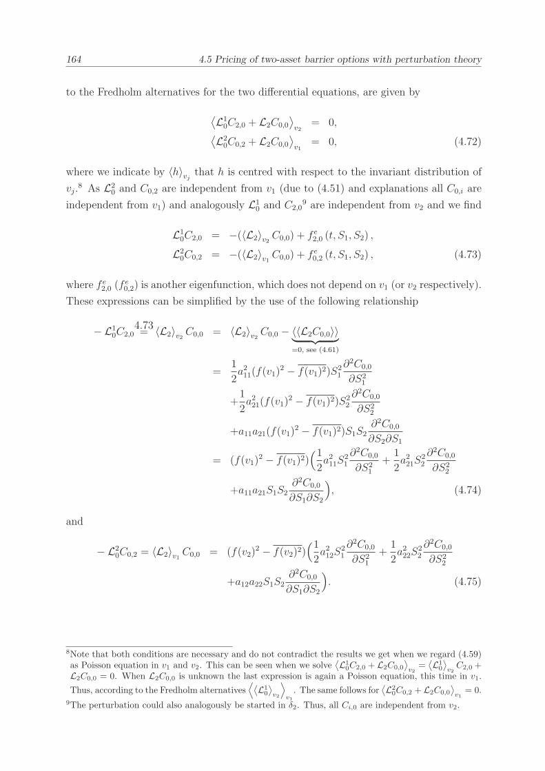
164 4.5 Pricing of two-asset barrier options with perturbation theory
to the Fredholm alternatives for the two differential equations, are given by
⟨L1
0C2,0 + L2C0,0
⟩
v2= 0,
⟨L2
0C0,2 + L2C0,0
⟩
v1= 0, (4.72)
where we indicate by 〈h〉vj that h is centred with respect to the invariant distribution of
vj.8 As L2
0 and C0,2 are independent from v1 (due to (4.51) and explanations all C0,i are
independent from v1) and analogously L10 and C2,0
9 are independent from v2 and we find
L10C2,0 = −(〈L2〉v2 C0,0) + f e
2,0 (t, S1, S2) ,
L20C0,2 = −(〈L2〉v1 C0,0) + f e
0,2 (t, S1, S2) , (4.73)
where f e2,0 (f
e0,2) is another eigenfunction, which does not depend on v1 (or v2 respectively).
These expressions can be simplified by the use of the following relationship
− L10C2,0
4.73= 〈L2〉v2 C0,0 = 〈L2〉v2 C0,0 − 〈〈L2C0,0〉〉
︸ ︷︷ ︸
=0, see (4.61)
=1
2a211(f(v1)
2 − f(v1)2)S21
∂2C0,0
∂S21
+1
2a221(f(v1)
2 − f(v1)2)S22
∂2C0,0
∂S22
+a11a21(f(v1)2 − f(v1)2)S1S2
∂2C0,0
∂S2∂S1
= (f(v1)2 − f(v1)2)
(1
2a211S
21
∂2C0,0
∂S21
+1
2a221S
22
∂2C0,0
∂S22
+a11a21S1S2∂2C0,0
∂S1∂S2
)
, (4.74)
and
− L20C0,2 = 〈L2〉v1 C0,0 = (f(v2)
2 − f(v2)2)(1
2a212S
21
∂2C0,0
∂S21
+1
2a222S
22
∂2C0,0
∂S22
+a12a22S1S2∂2C0,0
∂S1∂S2
)
. (4.75)
8Note that both conditions are necessary and do not contradict the results we get when we regard (4.59)as Poisson equation in v1 and v2. This can be seen when we solve
⟨L10C2,0 + L2C0,0
⟩
v2=⟨L10
⟩
v2C2,0 +
L2C0,0 = 0. When L2C0,0 is unknown the last expression is again a Poisson equation, this time in v1.
Thus, according to the Fredholm alternatives⟨⟨L10
⟩
v2
⟩
v1
. The same follows for⟨L20C0,2 + L2C0,0
⟩
v1= 0.
9The perturbation could also analogously be started in δ2. Thus, all Ci,0 are independent from v2.
4 Pricing of barrier options within stochastic correlation model 165
Further, we define φ as the solution of Poisson equations
(L10 + L2
0)φ =2∑
j=1
(f(vj)2 − f(vj)2), (4.76)
L10φ1 = f(v1)
2 − f(v1)2,L2
0φ2 = f(v2)2 − f(v2)2.
Hence, we can write with (4.76) and (4.73)
C2,0 = −1
2φ1
(
a211S21
∂2
∂S21
+ a221S22
∂2
∂S22
+ 2a11a21S1S2∂2
∂S1∂S2
)
C0,0
+f e2,0 (t, S1, S2) , (4.77)
C0,2 = −1
2φ2
(
a212S21
∂2
∂S21
+ a222S22
∂2
∂S22
+ 2a12a22S1S2∂2
∂S1∂S2
)
C0,0
+f e0,2 (t, S1, S2) . (4.78)
Equation (4.60) is a Poisson equation in v1, v2. As C0,3 is independent from v1 (due to
(4.51) and explanations all C0,i are independent from v1) and C2,1 is independent from
v210 we can reformulate (4.60):
(L20 + L1
0)(C0,3 + C2,1) = −(L21C0,2 + L2C0,1). (4.79)
Hence, the following statement must be imposed to guarantee the solvability of the Poisson
equation
〈〈L2〉〉C0,1 = −⟨⟨L2
1C0,2
⟩⟩= −
⟨L2
1C0,2
⟩
v2(4.80)
(4.78)=
⟨
L21
1
2φ2
(
a212S21
∂2
∂S21
+ a222S22
∂2
∂S22
+ 2a12a22S1S2∂2
∂S1∂S2
)
C0,0
⟩
v2
.
Applying (4.76) the problem for C0,1 can be simplified.
Corollary 19. (C0,1)
The problem for C0,1 is given by
LBS(σ1, σ2, ρ)C0,1 = A2C0,0,
C0,1 (T, S1, S2) = 0, (4.81)
10Due to (4.58) and the following explanations all C1,i are independent from v1. We get the analogousresult for Ci,1 being independent from v2 when we start the perturbation in δ2.
166 4.5 Pricing of two-asset barrier options with perturbation theory
with
A2 =
⟨√v2f(v2)
∂φ2
∂v2
⟩
v2
ρv2σv2
(a122S1
∂
∂S1
+a222S2
∂
∂S2
)
(
a212S21
∂2
∂S21
+ a222S22
∂2
∂S22
+ 2a12a22S1S2∂2
∂S1∂S2
)
, (4.82)
where ∂φ2
∂v2= − 2
σ2v2
v2p(v2)
∫ v2
0(f(z2)
2 − f(v2)2)p(z2)dz2 (see Equation (B.32)). Thus,
⟨√v2f(v2)
∂φ2
∂v2
⟩
v2
=
∫ ∞
0
√v2f(v2)
∂φ2
∂v2p(v2)dv2
= − 2
σ22,v
∫ ∞
0
∫ v2
0
f(v2)(f(z2)2 − f(v2)2)√v2
p(z2)dz2dv2.
If f(v2) =√v2
⟨√v2f(v2)
∂φ2
∂v2
⟩
v2
= − 2
σ22,v
∫ ∞
0
∫ v2
0
(z2 − v2)p(z2)dz2dv2
(B.28)= − 2
σ22,v
∫ ∞
0
(∫ v2
0
µCIRaCIR
Γ(aCIR)za
CIR
2 e−µCIRz2dz2 − v2)
dv2
= − 2
σ22,v
∫ ∞
0
(
1
µCIR
∫ v2
0
x(aCIR+1)−12
Γ(aCIR)e−x2dx2 − v2
)
dv2
= − 2
σ22,v
∫ ∞
0
(γ(aCIR + 1, µCIRv2)
Γ(aCIR)µCIR− v2
)
dv2, (4.83)
where γ(c, x) =∫ x
0e−ttc−1dt is the lower incomplete gamma function (see [59], 8.350 and
8.351).
It can be easily shown that
C0,1 = −(T − t)A2C0,0, (4.84)
as LBS commutes with Si∂k
∂Ski
for k = 1, 211 and LBSC0,0 = 0, i.e. LBS (−(T − t)A2C0,0) =
A2C0,0 − (T − t)A2LBSC0,0(4.61)= A2C0,0.
11For k = 1: Si∂
∂Si
(
S2i∂2C0,0
∂S2i
)
= Si
(
2Si∂2C0,0
∂S2i
+ S2i∂3C0,0
∂S3i
)
= S2i
∂2
∂S2i
(
Si∂C0,0
∂Si
)
4 Pricing of barrier options within stochastic correlation model 167
The PDE in the case of the barrier option is given by
LBS(σ1, σ2, ρ)CB,0,1 = A2CB,0,0,
CB,0,1 (T, S1, S2) = 0,
CB,0,1(t, B1(t), S2) = 0,
CB,0,1(t, S1, B2(t)) = 0.
We simplify the problem by defining (see [70])
CB,0,1 = CB,0,1 + V12S1∂2CB,0,0
∂f(v2)2∂S1
+ V22S2∂2CB,0,0
∂f(v2)2∂S2
. (4.85)
When we differentiate LBSCB,0,0 with respect to f(vj)2 we see
∂
∂f(vj)2(LBSCB,0,0) =
∂∂CB,0,0
∂f(vj)2
∂t+
1
2S21
2∑
j=1
a21jf(vj)2∂2
∂CB,0,0
∂f(vj)2
∂S21
+1
2S22
2∑
j=1
a22jf(vj)2∂2
∂CB,0,0
∂f(vj)2
∂S22
+ S1S2
2∑
j=1
a1ja2jf(vj)2∂2
∂CB,0,0
∂f(vj)2
∂S1∂S2
+r
S1
∂∂CB,0,0
∂f(vj)2
∂S1
+ S2
∂∂CB,0,0
∂f(vj)2
∂S2
− ∂CB,0,0
∂f(vj)2
+1
2
(
S21a
21j
∂2CB,0,0
∂S21
+ S22a
22j
∂2CB,0,0
∂S22
+ 2S1S2a1ja2j∂2CB,0,0
∂S1∂S2
)
= LBS
∂CB,0,0
∂f(vj)2+ (4.86)
+1
2
(
S21a
21j
∂2CB,0,0
∂S21
+ S22a
22j
∂2CB,0,0
∂S22
+ 2S1S2a1ja2j∂2CB,0,0
∂S1∂S2
)
= 0,

168 4.5 Pricing of two-asset barrier options with perturbation theory
due to Equation (4.67).12 Hence, LBS(σ1, σ2, ρ)∂CB,0,0
∂f(vj)2for j = 1, 2 solves the PDE problem
LBS
∂CB,0,0
∂f(vj)2= −1
2
(
S21a
21j
∂2CB,0,0
∂S21
+ S22a
22j
∂2CB,0,0
∂S22
+2S1S2a1ja2j∂2CB,0,0
∂S1∂S2
)
,
∂CB,0,0
∂f(vj)2(T, S1, S2) = 0,
∂CB,0,0
∂f(vj)2(t, B1(t), S2) = 0,
∂CB,0,0
∂f(vj)2(t, S1, B2(t)) = 0. (4.87)
Differentiating this with respect to Si with i = 1, 2 we see that due to the fact that LBS
commutes with Si∂k
∂Ski
for k = 1, 2,
LBS(Si
∂2CB,0,0
∂Si∂f(vj)2) = −1
2Si
∂
∂Si
(
S21a
21j
∂2CB,0,0
∂S21
+ S22a
22j
∂2CB,0,0
∂S22
+2S1S2a1ja2j∂2CB,0,0
∂S1∂S2
)
,
∂2CB,0,0
∂Si∂f(vj)2(T, Si, Sk) = 0,
∂2CB,0,0
∂Si∂f(vj)2(t, Bi(t), Sk) in general not 0,
∂2CB,0,0
∂Si∂f(vj)2(t, S1, Bk(t)) = 0. (4.88)
CB,0,1 is therefore the solution to the problem
LBS(σ1, σ2, ρ)CB,0,1 = 0,
CB,0,1 (T, S1, S2) = 0,
CB,0,1(t, B1(t), S2) = V12g12(t, B1, S2(t)),
CB,0,1(t, S1, B2(t)) = V22g22(t, S1(t), B2), (4.89)
12Note that with (4.62) LBSCB,0,0 =∂CB,0,0
∂t+ 1
2S21
∑2j=1 a
21jf(vj)
2 ∂2CB,0,0
∂S21
+ 12S
22
∑2j=1 a
22jf(vj)
2 ∂2CB,0,0
∂S22
+ S1S2
∑2j=1 a1ja2jf(vj)
2 ∂2CB,0,0
∂S1∂S2+ r
(
S1∂CB,0,0
∂S1+ S2
∂CB,0,0
∂S2− CB,0,0
)
= 0.
4 Pricing of barrier options within stochastic correlation model 169
where
V12 =
⟨√v2f(v2)
∂φ2
∂v2
⟩
v2
ρv2σv2a12, (4.90)
V22 =
⟨√v2f(v2)
∂φ2
∂v2
⟩
v2
ρv2σv2a22, (4.91)
g12(t, B1, S2(t)) = S1∂2CB,0,0
∂f(v2)2∂S1
∣∣∣∣S1=B1(ι1),S2=S2(ι1)
,
g22(t, S1(t), B2) = S2∂2CB,0,0
∂f(v2)2∂S2
∣∣∣∣S1=S1(ι2),S2=B2(ι2)
.
The solution can be found by (for the following results see [71].)
CB,0,1(t, S1, S2, B1, B2) =
∫ T
0
∫ ∞
0
e−c1b1−c2b2e−c2(σ2a′p sinβp)V12g12(t
′, B1, B2eσ2a
′p sinβp)
pxGBM
(ι′ ∈ dt′, θ′p = βp
)da′pdt
′
+
∫ T
0
∫ ∞
0
e−c1b1−c2b2e−c1(σ1a′p
√1−ρ2)V22g22(t
′, B1eσ1
√1−ρ2a′p , B2)
pxGBM
(ι′ ∈ dt′, θ′p = 0
)da′pdt
′, (4.92)
where r′p = a′p and θ′p = (0, βp).
pxGBM(ι′ ∈ dt′, z (ι′) ∈ ∂Y ) =πec1x1+c2x2−
∫ t′
tr(s)ds−α(t′−t)
β2pt
′a′pe
a′p2+r2p
2t′
∞∑
n=1
δnn
sin
(nπθpβp
)
Inπβp
(a′prp
t′
)
, (4.93)
where z describes the vector of transformed variables in polar coordinates, ∂Y describes
the boundary, i.e. the wedge with δn = 1 if θ′p = 0 (i.e. S2 = B2(t), S1 = ex′1K1 =
B1eσ1
√1−ρ2z′1 = B1e
σ1
√1−ρ2r′p cos(θ′p) = B1e
σ1
√1−ρ2r′p) and δn = (−1)n+1 if θ′p = βp (i.e.
S1 = B1(t),S2 = K2ex′2 = B2e
σ2z′2 = B2e
σ2r′p sin θ′p). tan βp = −
√1−ρ2
ρ, βp ∈ [0, π]. For
ρ = − cos πn, pxGBM(ι′ ∈ dt′, z(ι′) ∈ ∂Y ) can be attained in an easier way.
For θ′p = 0
pxGBM(ι′ ∈ dt′, z(ι′) ∈ ∂Y ) = ec1x1+c2x2−∫ t′
tr(s)ds−α(t′−t)
1
t′2
2n−1∑
k=0
(−1)kΦ(z′ − Tkz√
t)∣∣∣z′2=0
(e2Tkz′) ,
where e2 is the vector (0, 1), Φ is the standard normal distribution with 12πe−
(z′1−z1)2+(z′2−z2)
2
2 ,
170 4.5 Pricing of two-asset barrier options with perturbation theory
z′ = (z′1, z′2), z0 = (z1, z2),
Tkz =
(rp cos(2kπn
+ θp), rp sin(2kπn
+ θp)) for k even,
(rp cos(2(k−1)π
n− θp), rp sin(2(k−1)π
n− θp)) for k odd,
(4.94)
xi = ln
(
Sie∫ Tt
rds
Ki
)
,
z1 =1
√
1− ρ2
(x1 − b1σ1
− ρ(x2 − b2σ2
))
,
z2 =x2 − b2σ2
.
For θ′p = βp
pxGBM(ι′ ∈ dt′, z(ι′) ∈ ∂Y ) = ec1x1+c2x2−∫ t′
tr(s)ds−α(t′−t)
1
t′2
2n−1∑
k=0
(−1)kΦ(z′ − Tkz√
t)∣∣∣z′2=0
(e2Tkz′) ,
with θp = βp − θp and
Tkz =
(rp cos(2kπn
+ θp), rp sin(2kπn
+ θp)) for k even,
(rp cos(2(k−1)π
n− θp), rp sin(2(k−1)π
n− θp)) for k odd.
(4.95)
Corollary 20. (CB,0,1)
The solution for CB,0,1 is given by
CB,0,1 = CB,0,1 − V12S1∂2CB,0,0
∂f(v2)2∂S1
− V22S2∂2CB,0,0
∂f(v2)2∂S2
. (4.96)
Solving the PDE for the first-order corrections C1,0 and CB,1,0
Inserting expression (4.56) in (4.54) and collecting terms of the same order of δ2 we obtain
the following relationships
δ−22 : L2
0C1,0 = 0, (4.97)
δ−12 : L2
0C1,1 + L21C1,0 = 0, (4.98)
δ02 : L20C1,2 + L2
1C1,1 + L2C1,0 + L11C2,0 + L1
0C3,0 = 0, (4.99)
δ12 : L20C1,3 + L2
1C1,2 + L2C1,1 + L11C2,1 + L1
0C3,1 = 0. (4.100)

4 Pricing of barrier options within stochastic correlation model 171
We notice that C1,0 and C1,1 are both independent from v2. Equation (4.99) is a Poisson
equation in v1, v2 while L21C1,1 = 0.
As L20C3,0 = 0 due to the independence of C3,0 from v2 (due to (4.51) and explanations all
C0,i are independent from v1. The same follows analogously for Ci,0 as the perturbation
could be also started with δ2.) and L10C1,2 = 0 because C1,2 is independent from v1 (due
to (4.52) and the respective explanations) we can reformulate (4.99)
(L2
0 + L10
)(C1,2 + C3,0) = −
(L1
1C2,0 + L2C1,0
). (4.101)
The following condition has to be fulfilled so that this Poisson equation is solvable:
〈〈L2〉〉C1,0 = −⟨⟨L1
1C2,0
⟩⟩ (4.77)= −
⟨L1
1C2,0
⟩
v1. (4.102)
Using (4.76) and (4.77) the respective problem for C1,0 can be found.
Corollary 21. (C1,0)
C1,0 solves the following problem
LBS(σ1, σ2)C1,0 = A1C0,0,
C1,0 (T, S1, S2) = 0, (4.103)
where
A1 =
⟨√v1f(v1)
∂φ1
∂v1
⟩
v1
ρv1σv1
(a112S1
∂
∂S1
+a212S2
∂
∂S2
)
(
a211S21
∂2
∂S21
+ a221S22
∂2
∂S22
+ 2a11a21S1S2∂2
∂S1∂S2
)
. (4.104)
Analogously to (4.84) the solution for the two-asset option without barriers can be easily
indicated by
C1,0 = −(T − t)A1C0,0. (4.105)
Accordingly, the problem for the barrier option is given by
LBS(σ1, σ2, ρ)CB,1,0 = A1CB,0,0,
CB,1,0 (T, S1, S2) = 0,
CB,1,0(t, B1(t), S2) = 0,
CB,1,0(t, S1, B2(t)) = 0. (4.106)

172 4.5 Pricing of two-asset barrier options with perturbation theory
We redefine the problem analogously to (4.87)-(4.88) by
CB,1,0 = CB,1,0 + V11S1∂2CB,0,0
∂f(v1)2∂S1
+ V21S2∂2CB,0,0
∂f(v1)2∂S2
. (4.107)
CB,1,0 is the solution to the problem
LBS(σ1, σ2)CB,1,0 = 0,
CB,1,0 (T, S1, S2) = 0,
CB,1,0(t, B1(t), S2) = V11g11(t, B1, S2(t)),
CB,1,0(t, S1, B2(t)) = V21g21(t, S1, B2(t)), (4.108)
where
V11 =1
2
⟨√v1f(v1)
∂φ1
∂v1
⟩
v1
ρv1σ1,va11, (4.109)
V21 =1
2
⟨√v1f(v1)
∂φ1
∂v1
⟩
v1
ρv1σ1,va21, (4.110)
g11(t, B1, S2(t)) = S1∂2CB,0,0
∂f(v1)2∂S1
∣∣∣∣S1=B1(ι1),S2=S2(ι1)
,
g21(t, S1, B2(t)) = S2∂2CB,0,0
∂f(v1)2∂S2
∣∣∣∣S1=S1(ι2),S2=B2(ι2)
.
Analogously to (4.92) the solution can be found by
CB,1,0(t, S1, S2, B1, B2) =
∫ T
0
∫ ∞
0
e−c1b1−c2b2e−c2(σ2a′p sinβp)V12g11(t
′, B1, B2eσ2a
′p sinβp)
pxGBM
(ι′ ∈ dt′, θ′p = βp
)da′pdt
′
+
∫ T
0
∫ ∞
0
e−c1b1−c2b2e−c1(σ1a′p
√1−ρ2)V22g21(t
′, B1eσ1
√1−ρ2a′p , B2)
pxGBM
(ι′ ∈ dt′, θ′p = 0
)da′pdt
′, (4.111)
where the probability is given in (4.93).
Corollary 22. CB,1,0
The solution to CB,1,0 is given by
CB,1,0 = CB,1,0 − V11S1∂2CB,0,0
∂f(v1)2∂S1
− V21S2∂2CB,0,0
∂f(v1)2∂S2
. (4.112)
4 Pricing of barrier options within stochastic correlation model 173
Solving the PDE for the first-order corrections C1,1 and CB,1,1
Equation (4.99) is a Poisson equation with respect to v1 for C3,0. Thus, we deduce with
(4.102)
L20C1,2 = −
⟨L1
1C2,0 + L2C1,0
⟩
v1
(4.102)= −
(−〈〈L2〉〉C1,0 + 〈L2〉v1 C1,0
)
(4.105)=
1
2(T − t)(f(v2)2 − f(v2)2)(
a212S21
∂2
∂S21
+ a222S22
∂2
∂S22
+ 2a12a22S1S2∂2
∂S1∂S2
)
A1C0,0, (4.113)
C1,2 =1
2(T − t)φ2
(
a212S21
∂2
∂S21
+ a222S22
∂2
∂S22
+ 2a12a22S1S2∂2
∂S1∂S2
)
A1C0,0
+f e1,2 (t, S1, S2) ,
where f e1,2 (t, S1, S2) is another eigenfunction, which does not depend on v1. In this way,
Equation (4.60) is a Poisson equation in v2 for C0,3. Hence, from the solvability condition
together with (4.80) follows, analogue to (4.113):
L10C2,1 = −
⟨L2
1C0,2 + L2C0,1
⟩
v2
=1
2(T − t)(f(v1)2 − f(v1)2)(
a211S21
∂2
∂S21
+ a221S22
∂2
∂S22
+ 2a11a21S1S2∂2
∂S1∂S2
)
A2C0,0, (4.114)
C2,1 =1
2(T − t)φ1
(
a211S21
∂2
∂S21
+ a221S22
∂2
∂S22
+ 2a11a21S1S2∂2
∂S1∂S2
)
A2C0,0
+f e2,1 (t, S1, S2) ,
where f e2,1 (t, S1, S2) is another eigenfunction, which does not depend on v2. Finally,
Equation (4.100) is a Poisson equation in v1 and v2 for C3,1 and C1,3. To ensure its
solvability we have to enforce the following condition
〈〈L2〉〉C1,1 = −⟨⟨L2
1C1,2 + L11C2,1
⟩⟩.
Corollary 23. (C1,1)
C1,1 satisfies the following problem
〈〈L2〉〉C1,1 = 2(t− T )A1A2C0,0. (4.115)

174 4.5 Pricing of two-asset barrier options with perturbation theory
Concluding, as in (4.84) and (4.105),
C1,1 = (T − t)2A1A2C0,0. (4.116)
This result can be easily checked by inserting (4.116) in (4.115).
For the barrier option the problem is given by
LBS(σ1, σ2, ρ)CB,1,1 = 2(T − t)A1A2CB,0,0,
CB,1,1 (T, S1, S2) = 0,
CB,1,1(t, B1(t), S2) = 0,
CB,1,1(t, S1, B2(t)) = 0. (4.117)
In order to simplify the problem we deduce that
LBS
((T − t)2A1A2CB,0,0
)= −2(T − t)A1A2CB,0,0 + (T − t)2LBSA1A2CB,0,0
︸ ︷︷ ︸
=0
, (4.118)
the last term equals zero as A1 and A2 commutes with LBS. Hence, we define
CB,1,1 = CB,1,1 + (T − t)2A1A2CB,0,0 (4.119)
CB,1,1 is the solution to the problem
LBS(σ1, σ2)CB,1,1 = 0,
CB,1,1 (T, S1, S2) = 0,
CB,1,1(t, B1(t), S2) = g1(t, B1, S2),
CB,1,1(t, S1, B2(t)) = g2(t, S1, B2), (4.120)
where
g1(t, B1, S1) = (T − t)2A1A2CB,0,0
∣∣∣∣S1=B1,S2=S2(ι1)
,
g2(t, S1, B2) = (T − t)2A1A2CB,0,0
∣∣∣∣S1=S1(ι2),S2=B2
. (4.121)
4 Pricing of barrier options within stochastic correlation model 175
The solution can be found by
CB,1,1 (t, S1, S2, B1, B2) =
∫ T
0
∫ ∞
0
e−c1b1−c2b2e−c2(σ2a′p sinβp)g1(t
′, B1, B2eσ2a
′p sinβp)
pxGBM
(ι′ ∈ dt′, θ′p = βp
)da′pdt
′
+
∫ T
0
∫ ∞
0
e−c1b1−c2b2e−c1(σ1a′p
√1−ρ2)g2(t
′, B1eσ1
√1−ρ2a′p , B2)
pxGBM
(ι′ ∈ dt′, θ′p = 0
)da′pdt
′, (4.122)
where the probability is given in (4.93).
Corollary 24. (CB,1,1)
The solution for CB,1,1 given by
CB,1,1 = CB,1,1 − (T − t)2A1A2CB,0,0. (4.123)
Accuracy of the approximation
We derive the accuracy of the price approximation along the lines of Fouque et al [52],
[49]. Each call or digital option has a payoff function which is only C0 smooth with a
discontinuous first derivative at the kink Si = Ki. However, for the proof we require a
smooth payoff function and smooth derivatives.
Thus, in order to proceed we regularise the payoff, which is a two-asset option, by replacing
it with the Black-Scholes price CBS of the two-asset option with time to maturity ǫ with
volatilities σ1, σ2 and correlation ρ, i.e. deterministic covariance because at t < T the
Black-Scholes price CBS is smooth, and the derivatives are well-defined.
We define therefore
gǫ (S1, S2) = CBS (T, S1, S2, K1, K2, T + ǫ, σ1, σ2, ρ) , (4.124)
with
CBS (t, S1, S2, K1, K2, T, σ1, σ2, ρ) = C0,0 (t, S1, S2, K1, K2, T, σ1, σ2, ρ) .
(4.125)
176 4.5 Pricing of two-asset barrier options with perturbation theory
Hence, the regularised price C ǫ,δ solves
LδC ǫ,δ = 0,
C ǫ,δ (T, S1, S2) = gǫ(S1, S2).
Let Qǫ,δ denote the first-order approximation to the regularised option price, i.e.
Qǫ,δ ≡ C ǫ0,0 + δ1C
ǫ1,0 + δ2C
ǫ0,1 + δ1δ2C
ǫ1,1, (4.126)
where
C ǫ0,0 (t, S1, S2) = CBS (t, S1, S2, K1, K2, T + ǫ, σ1, σ2, ρ) , (4.127)
C ǫ1,0 = −(T − t)A1C
ǫ0,0, (4.128)
C ǫ0,1 = −(T − t)A2C
ǫ0,0, (4.129)
C ǫ1,1 = (T − t)2A1A2C
ǫ0,0. (4.130)
Concluding, the proof must involve three steps. First, we show that the regularised price,
C ǫ,δ, is converging to the actual unregularised price, Cδ (see Lemma 2), in a next step we
deduct that the regularised approximation Qǫ,δ is close to the approximation Qδ, which
is defined in Equation (4.48), (see Lemma 3). Finally, it is left to prove that C ǫ,δ ∼ Qǫ,δ
in Lemma 4.
Lemma 2. (C ǫ,δ ∼ Cδ)
For the fixed point (t, S1, S2, v), where t < T and v = (v1, v2), there exist constants δ1
1 > 0,
δ1
2 > 0, ǫ1 > 0, and c1 > 0 such that
∣∣Cδ(t, S1, S2, v)− C ǫ,δ(t, S1, S2, v)
∣∣ ≤ c1ǫ, (4.131)
for all 0 < δ1 < δ1
1, 0 < δ2 < δ1
2, and 0 < ǫ < ǫ1.
Proof.
In the following we show that C ǫ,δ and Cδ converge to each other by conditioning the
difference in the prices on the paths of the eigenvectors up to T . For that we use the
probabilistic representation of the price as the risk-neutral value of the discounted payoff.
For the proof of this lemma we introduce the processes for Si, i ∈ (1, 2) with ρvj :
dSi = rSidt+ Si
2∑
j=1
aijf(vj(t))(√
1− ρvj 2dWj + ρvjdZj
)
, i = 1, 2, (4.132)
4 Pricing of barrier options within stochastic correlation model 177
where
f(vj(t)) =
f(vj(t)) for t ≤ T
f(vj)2 for t > T(4.133)
and vj follows the process described in (4.2). Note that Wj and Zj are two independent
Brownian motions with Zj = Zj in (4.2) and Wj = 1√1−ρvj
2(Wj − ρvjZj) in (4.1). The
assumption of a risk-neutral equivalent martingale measure allows for the probabilistic
representation of the price as the expected discounted payoff. Thus, we find
C ǫ,δ = EQ
[
e−r(T−t+ǫ)g(
S1(T + ǫ), S2(T + ǫ))]
,
Cδ = EQ
[
e−r(T−t)g(
S1(T ), S2(T ))]
.
In the next step we condition the difference of the regularised and the unregularised prices
on the paths of the Brownian motions of the eigenvalues follow, i.e.
C ǫ,δ − Cδ = EQ
[
E
[
e−r(T−t+ǫ)g(
S1 (T + ǫ) , S2(T + ǫ))
−e−r(T−t)g(
S1(T ), S2(T )) ∣∣Zj(s)t≤s≤T , j = 1, 2
]]
. (4.134)
To calculate the expectations we determine the conditional joint distribution of S1 and
S2. We start with the expectation in T and obtain the following diffusions for ln(S1) and
ln(S2):
d(
ln(S1))
= rdt− 1
2
2∑
j=1
a21jf(vj(t))2(1− ρvj 2)dt−
1
2
2∑
i=1
a21jf(vj(t))2ρvj
2dt
+2∑
j=1
a1jf(vj(t))√
1− ρvj 2dWj +2∑
j=1
a1jf(vj(t))ρvjdZj,
d(
ln(S2))
= rdt− 1
2
2∑
j=1
a22jf(vj(t))2(1− ρvj 2)dt−
1
2
2∑
j=1
a22jf(vj(t))2ρvj
2dt
+2∑
j=1
a2jf(vj(t))√
1− ρvj 2dWj +2∑
j=1
a2jf(vj(t))ρvjdZj,
178 4.5 Pricing of two-asset barrier options with perturbation theory
or
S1(T ) = S1(t)eΛ1 exp
r(T − t)− 1
2
∫ T
t
2∑
j=1
a21jf(vj(s))2(1− ρvj 2)ds
+2∑
j=1
∫ T
t
a1jf(vj(s))√
1− ρvj 2dWj
,
S2(T ) = S2(t)eΛ2 exp
r(T − t)− 1
2
∫ T
t
2∑
j=1
a22jf(v1(s))2(1− ρvj 2)ds
+2∑
j=1
∫ T
t
a2jf(vj(s))√
1− ρvj 2dWj
,
where
Λi =
∫ T
t
2∑
j=1
aijf(vj(s))ρvjdZj −
1
2
∫ T
t
2∑
j=1
a2ijf(vj(s))2ρvj
2ds. (4.135)
vj, j = 1, 2, i.e. vj, j = 1, 2, t ≤ T are independent from(
Wj(s))
0≤s≤Tunder Q as we
have reformulated the processes with independent Brownian motions(
Wj(s))
0≤s≤Tand
(Zj(s))0≤s≤T(see (4.132)). The conditional distribution of S1(T ) (S2(T ) respectively) is,
thus,
ln
(
S1(T )
S1(t)
)
∣∣Zj(s)t≤s≤T ∼ N
(
r(T − t) + Λ1 −1
2σ21, σ1
)
, (4.136)
with
σ2i = σ2
i (t, T ),
=
∫ T
t
((1− ρv21
)a2i1f(v1(s))
2 +(1− ρv22
)a2i2f(v2(s))
2)ds. (4.137)
To summarise we obtain the following conditional joint distribution
F(
ln(
S1
)
, ln(
S2
) ∣∣Zj(s)t≤s≤T , j = 1, 2
)
for ln(S1) and ln(S2) (for a single under-
lying see [103])
F(
ln(
S1(T ))
, ln(
S2(T )) ∣∣Zj(s)t≤s≤T , j = 1, 2
)
= N2
(m1,m2, σ
21, σ
22, ρ), (4.138)
where
mi = ln (Si(0)) + Λi + r(T − t)− 1
2σ2i , (4.139)
ρ =
∫ T
t(a11a21(1− ρv12)f(v1(s))2 + a12a22(1− ρv22)f(v2(s))2)ds
σ1σ2. (4.140)
4 Pricing of barrier options within stochastic correlation model 179
It follows that
E
[
e−r(T−t)g(S1(T ), S2(T ))∣∣Zj(s)t≤s≤T , j = 1, 2
]
= CBS
(
t, S1eΛ1 , S2e
Λ2 , K1, K2, T,σ1√T − t
,σ2√T − t
, ρ
)
. (4.141)
Accordingly, we get
F(
ln(
S1 (T + ǫ))
, ln(
S2 (T + ǫ)) ∣∣Zj(s)t≤s≤T , j = 1, 2
)
= N2
(m1, m2, σ
21, σ
22, ρ), (4.142)
where
mi = ln (Si(0)) + Λi + r(T − t) + rǫ− 1
2σ2i , (4.143)
σ2i = σi(t, T + ǫ)2
(4.133,4.137)= σi(t, T )
2 +
∫ T+ǫ
T
(
a2i1f(v1(s))2 + a2i2f(v2(s))
2)
(4.64)= σ2
i + ǫσ2i , (4.144)
ρ = ρ(t, T + ǫ)
(4.140)=
ρ(t, T )σ1(t, T )σ2(t, T ) +∫ T+ǫ
T(a11a21f(v1(s))2 + a12a22f(v2(s))2)ds
σ1(t, T + ǫ)σ2(t, T + ǫ)
(4.64)=
ρσ1σ2 + ǫρ σ1 σ2
σ1σ2. (4.145)
The conditional expectation can be computed by
E
[
e−r(T−t+ǫ)g(
S1(T + ǫ), S2 (T + ǫ)) ∣∣Zj(s)t≤s≤T , j = 1, 2
]
= e−rǫCδBS
(
t, S1eΛ1+rǫ, S2e
Λ2+rǫ, K1, K2, T,σ1√T − t
,σ2√T − t
, ρ
)
. (4.146)
Using the explicit formulas and the assumption that σi, i = 1, 2, is bounded above and
below (for detailed calculations see (B.2)), we derive that
∣∣∣e−rǫCBS
(t, S1e
Λ1+rǫ, S2eΛ2+rǫ, σ1, σ2, ρ
)− C ǫ,δ
BS
(t, S1e
Λ1 , S2eΛ2 , σ1, σ2, ρ
)∣∣∣
≤ ǫc4 (1 + |Λ1|+ |Λ2|+ |Λ1| |Λ2|)(eΛ2 + 1
). (4.147)
E(T ) := eΛi is the stochastic exponential of γ(T ) =∫ T
t
∑p
j=1 ρvjf(vj)aij because eΛi =
eγ(T )− 12〈γ,γ〉 and dE = Edγ. The expectation of the exponential martingale exists if the
Novikov condition is fulfilled, i.e. if E[
e12
∫ Tt ||√vj||2ds] <∞, which is the case for the CIR

180 4.5 Pricing of two-asset barrier options with perturbation theory
process (see [29]). We find
∣∣Cδ(t, S1, S2, v)− C ǫ,δ(t, S1, S2, v)
∣∣ ≤ c1ǫ, (4.148)
for c1 and ǫ small enough.
Lemma 3. (Qǫ,δ ∼ Qδ)
For the fixed point (t, S1, S2, v), where t < T and v = (v1, v2), there exist constants δ2
1 > 0,
δ2
2 > 0, ǫ2 > 0, and c2 > 0 such that
∣∣Qδ (t, S1, S2,v)−Qǫ,δ (t, S1, S2,v)
∣∣ ≤ c2ǫ, (4.149)
for all 0 < δ1 < δ2
1, 0 < δ2 < δ2
2, and 0 < ǫ < ǫ2.
Proof.
In the following we show that the approximation Qǫ,δ of the regularised payoff is close to
Qδ, the approximation of the unregularised payoff. From the definitions of the correction
terms C1,0 (see (4.105)), C0,1 (see (4.84)), and C1,1 (see (4.116)) it follows that
Qǫ,δ −Qδ =(1− (T − t) (δ1A1 + δ2A2) + (T − t)2δ1δ2A1A2
) (C ǫ
0,0 − C0,0
).
From the definition of A1 (see (4.104)) and A2 (see (4.82)) one can see that they are
bounded due to the boundedness of the solutions of the Poisson equations in v1 and v2
(see (B.3)).
As C ǫ0,0 (t, T, S1, S2) = C0,0(t, T + ǫ, S1, S2) and C0,0 as well as its successive derivatives
with respect to S1 and S2 are differentiable in t at any t < T we deduce for (t, S1, S2, v)
with fixed t < T :
|Qδ −Qδ,ǫ| ≤ c2ǫ, (4.150)
for some c2 > 0 and ǫ small enough.
Lemma 4. (C ǫ,δ ∼ Qǫ,δ)
For the fixed point (t, S1, S2, v), where t < T and v = (v1, v2), there exist constants δ3
1 > 0,
δ3
2 > 0, ǫ2 > 0, and c3 > 0 such that
∣∣C ǫ,δ(t, S1, S2, v)−Qǫ,δ(t, S1, S2, v)
∣∣ ≤ c3
(
δ21
(
1 + ǫ−12 + δ1ǫ
−1)
(4.151)
+δ22
(
1 + ǫ−12 + δ2ǫ
−1)
δ1δ2
(
1 + ǫ−12 + δ1ǫ
−1 + δ2ǫ−1))
,

4 Pricing of barrier options within stochastic correlation model 181
for all 0 < δ1 < δ3
1, 0 < δ2 < δ3
2, and 0 < ǫ < ǫ3.
Proof.
In the following we show that the regularised approximation Qǫ,δ converges to the actual
regularised price C ǫ,δ by finding a boundary for the absolute value of the error in the
approximation, Rǫ,δ. We first introduce C ǫ,δ, which we define by
C ǫ,δ = Qǫ,δ + δ21Cǫ2,0 + δ22C
ǫ0,2 + δ21δ2C
ǫ2,1 + δ1δ
22C
ǫ1,2 + δ31C
ǫ3,0 + δ32C
ǫ0,3, (4.152)
and, thus, define the error in the approximation for the regularised problem as
Rǫ,δ = C ǫ,δ − C ǫ,δ. (4.153)
By applying Lδ on Rǫ,δ and forming terms of equal power in δ1 and δ2 we see that
LδRǫ,δ = Lδ(C ǫ,δ − C ǫ,δ)
=1
δ21L1
0Cǫ0,0 +
1
δ1
(L1
0Cǫ1,0 + L1
1Cǫ0,0
)
+1
δ22L2
0Cǫ0,0 +
1
δ2
(L2
0Cǫ0,1 + L2
1Cǫ0,0
)
+(L2
0Cǫ0,2 + L2
1Cǫ0,1 + L2C
ǫ0,0 + L1
0Cǫ2,0
)
+δ2(L2
0Cǫ0,3 + L2
1Cǫ0,2 + L2C
ǫ0,1 + L1
0Cǫ2,1
)
+δ1δ22L2
0Cǫ1,0 +
δ1δ2(L2
0Cǫ1,1 + L2
1Cǫ1,0)
+δ1(L2
0Cǫ1,2 + L2
1Cǫ1,1 + L2C
ǫ1,0 + L1
0Cǫ2,0 + L1
1Cǫ2,0
)
+δ2δ21L1
0Cǫ0,1 +
δ2δ1
(L1
0Cǫ1,1 + L1
1Cǫ0,1
)
+δ1δ2(L2
1Cǫ1,2 + L2C
ǫ1,1 + L1
1Cǫ2,1
)
+δ21(L2C
ǫ2,0 + δ2L2C
ǫ2,1 + L1
1Cǫ3,0 + δ1L2C
ǫ3,0
)
+δ22(L2C
ǫ0,2 + δ1L2C
ǫ1,2 + L2
1Cǫ0,3 + δ2L2C
ǫ0,3
)
= δ1δ2Fǫ1 (t, S1, S2,v) + δ21F
ǫ2 (t, S1, S2,v)
+δ22Fǫ3 (t, S1, S2,v) , (4.154)
because LδC ǫ,δ = 0 and the first approximations are chosen to cancel the first brackets
(see (4.51)-(4.54) and (4.57)-(4.60)). We define
F ǫ1 (t, S1, S2,v) = L2
1Cǫ1,2 + L2C
ǫ1,1 + L1
1Cǫ2,1 + δ1L2C
ǫ2,1 + δ2L2C
ǫ1,2,
F ǫ2 (t, S1, S2,v) = L2C
ǫ2,0 + L1
1Cǫ3,0 + δ1L2C
ǫ3,0,
F ǫ3 (t, S1, S2,v) = L2C
ǫ0,2 + L2
1Cǫ0,3 + δ2L2C
ǫ0,3. (4.155)
182 4.5 Pricing of two-asset barrier options with perturbation theory
The derivation of C3,0 and C0,3 is shown in the Appendix B.2. From Equations (4.77,
4.78, 4.113, 4.114) we moreover deduce
C ǫ0,2 = −1
2φ2
(
a212S21
∂2
∂S21
+ a222S22
∂2
∂S22
+ 2a12a22S1S2∂2
∂S1∂S2
)
C ǫ0,0
+f0,2e,ǫ (t, S1, S2) ,
C ǫ2,0 = −1
2φ1
(
a211S21
∂2
∂S21
+ a221S22
∂2
∂S22
+ 2a11a21S1S2∂2
∂S1∂S2
)
C ǫ0,0
+f2,0e,ǫ (t, S1, S2) ,
C ǫ1,2 =
1
2(T − t)φ2
(
a212S21
∂2
∂S21
+ a222S22
∂2
∂S22
+ 2a12a22S1S2∂2
∂S1∂S2
)
A1Cǫ0,0
+f1,2e,ǫ (t, S1, S2) ,
C ǫ2,1 =
1
2(T − t)φ1
(
a211S21
∂2
∂S21
+ a221S22
∂2
∂S22
+ 2a11a21S1S2∂2
∂S1∂S2
)
A2Cǫ0,0
+f2,1e,ǫ (t, S1, S2) ,
C ǫ0,3 =
1
2(T − t)φ2
(
a212S21
∂2
∂S21
+ a222S22
∂2
∂S22
+ 2a12a22S1S2∂2
∂S1∂S2
)
A2Cǫ0,0
+ρ2σ2vξ2
(
S1a122
∂
∂S1
+ S2a222
∂
∂S2
)
(
a212S21
∂2
∂S21
+ a222S22
∂2
∂S22
+ 2a12a22S1S2∂2
∂S1∂S2
)
C ǫ0,0
+f0,3e,ǫ (t, S1, S2) ,
C ǫ3,0 =
1
2(T − t)φ1
(
a211S21
∂2
∂S21
+ a221S22
∂2
∂S22
+ 2a11a21S1S2∂2
∂S1∂S2
)
A1Cǫ0,0
+ρ1σ1vξ1
(
S1a112
∂
∂S1
+ S2a212
∂
∂S2
)
(
a211S21
∂2
∂S21
+ a221S22
∂2
∂S22
+ 2a11a21S1S2∂2
∂S1∂S2
)
C ǫ0,0
+f3,0e,ǫ (t, S1, S2) , (4.156)
where
(L10 + L2
0)ξ =2∑
i=1
(
√vif(vi)
∂φi
∂vi−⟨√
vif(vi)∂φi
∂vi
⟩
vi
)
, (4.157)
L10ξ1 =
√v1f(v1)
∂φ1
∂v1−⟨√
v1f(v1)∂φ1
∂v1
⟩
v1
,
L20ξ2 =
√v2f(v2)
∂φ2
∂v2−⟨√
v2f(v2)∂φ2f
∂v2
⟩
v2
.
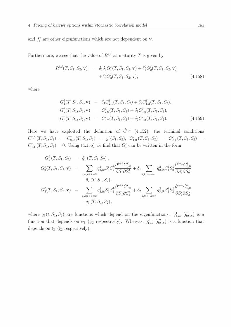
4 Pricing of barrier options within stochastic correlation model 183
and f ei are other eigenfunctions which are not dependent on v.
Furthermore, we see that the value of Rǫ,δ at maturity T is given by
Rǫ,δ(T, S1, S2,v) = δ1δ2Gǫ1(T, S1, S2,v) + δ21G
ǫ2(T, S1, S2,v)
+δ22Gǫ3(T, S1, S2,v), (4.158)
where
Gǫ1(T, S1, S2,v) = δ1C
ǫ2,1(T, S1, S2) + δ2C
ǫ1,2(T, S1, S2),
Gǫ2(T, S1, S2,v) = C ǫ
2,0(T, S1, S2) + δ1Cǫ3,0(T, S1, S2),
Gǫ3(T, S1, S2,v) = C ǫ
0,2(T, S1, S2) + δ2Cǫ0,3(T, S1, S2). (4.159)
Here we have exploited the definition of C ǫ,δ (4.152), the terminal conditions
C ǫ,δ (T, S1, S2) = C ǫ0,0 (T, S1, S2) = gǫ(S1, S2), C ǫ
1,0 (T, S1, S2) = C ǫ0,1 (T, S1, S2) =
C ǫ1,1 (T, S1, S2) = 0. Using (4.156) we find that Gǫ
i can be written in the form
Gǫ1 (T, S1, S2) = q1 (T, S1, S2) ,
Gǫ2(T, S1, S2,v) =
∑
i,k;i+k=2
q12,ikSi1S
k2
∂i+kC ǫ0,0
∂Si1∂S
k2
+ δ1∑
i,k;i+k=3
q22,ikSi1S
k2
∂i+kC ǫ0,0
∂Si1∂S
k2
+q2 (T, S1, S2) ,
Gǫ3(T, S1, S2,v) =
∑
i,k;i+k=2
q13,ikSi1S
k2
∂i+kC ǫ0,0
∂Si1∂S
k2
+ δ2∑
i,k;i+k=3
q23,ikSi1S
k2
∂i+kC ǫ0,0
∂Si1∂S
k2
+q3 (T, S1, S2) ,
where qi (t, S1, S2) are functions which depend on the eigenfunctions. q11,ik (q12,ik) is a
function that depends on φ1 (φ2 respectively). Whereas, q21,ik (q22,ik) is a function that
depends on ξ1 (ξ2 respectively).
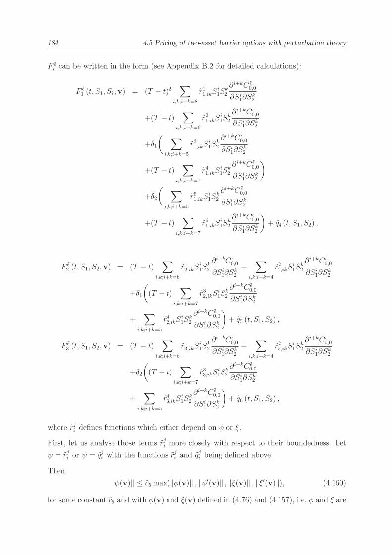
184 4.5 Pricing of two-asset barrier options with perturbation theory
F ǫi can be written in the form (see Appendix B.2 for detailed calculations):
F ǫ1 (t, S1, S2,v) = (T − t)2
∑
i,k;i+k=8
r11,ikSi1S
k2
∂i+kC ǫ0,0
∂Si1∂S
k2
+(T − t)∑
i,k;i+k=6
r21,ikSi1S
k2
∂i+kC ǫ0,0
∂Si1∂S
k2
+δ1
(∑
i,k;i+k=5
r31,ikSi1S
k2
∂i+kC ǫ0,0
∂Si1∂S
k2
+(T − t)∑
i,k;i+k=7
r41,ikSi1S
k2
∂i+kC ǫ0,0
∂Si1∂S
k2
)
+δ2
(∑
i,k;i+k=5
r51,ikSi1S
k2
∂i+kC ǫ0,0
∂Si1∂S
k2
+(T − t)∑
i,k;i+k=7
r61,ikSi1S
k2
∂i+kC ǫ0,0
∂Si1∂S
k2
)
+ q4 (t, S1, S2) ,
F ǫ2 (t, S1, S2,v) = (T − t)
∑
i,k;i+k=6
r12,ikSi1S
k2
∂i+kC ǫ0,0
∂Si1∂S
k2
+∑
i,k;i+k=4
r22,ikSi1S
k2
∂i+kC ǫ0,0
∂Si1∂S
k2
+δ1
(
(T − t)∑
i,k;i+k=7
r32,ikSi1S
k2
∂i+kC ǫ0,0
∂Si1∂S
k2
+∑
i,k;i+k=5
r42,ikSi1S
k2
∂i+kC ǫ0,0
∂Si1∂S
k2
)
+ q5 (t, S1, S2) ,
F ǫ3 (t, S1, S2,v) = (T − t)
∑
i,k;i+k=6
r13,ikSi1S
k2
∂i+kC ǫ0,0
∂Si1∂S
k2
+∑
i,k;i+k=4
r23,ikSi1S
k2
∂i+kC ǫ0,0
∂Si1∂S
k2
+δ2
(
(T − t)∑
i,k;i+k=7
r33,ikSi1S
k2
∂i+kC ǫ0,0
∂Si1∂S
k2
+∑
i,k;i+k=5
r43,ikSi1S
k2
∂i+kC ǫ0,0
∂Si1∂S
k2
)
+ q6 (t, S1, S2) ,
where rji defines functions which either depend on φ or ξ.
First, let us analyse those terms rji more closely with respect to their boundedness. Let
ψ = rji or ψ = qji with the functions rji and qji being defined above.
Then
‖ψ(v)‖ ≤ c5 max(‖φ(v)‖ , ‖φ′(v)‖ , ‖ξ(v)‖ , ‖ξ′(v)‖), (4.160)
for some constant c5 and with φ(v) and ξ(v) defined in (4.76) and (4.157), i.e. φ and ξ are

4 Pricing of barrier options within stochastic correlation model 185
the solutions of Poisson equations with h = f(v)2−f(v)2 or h =√vf(v)∂φ
∂v−⟨√
vf(v)∂φ∂v
⟩.
Due to the results in Appendix B.3 ψ is at most logarithmically growing in v at infinity
(see Appendix B.3). As the moments of the process of v are uniformly bounded in
δ = (δ1, δ2) (see Section 2.4.1) we can conclude that there exists a constant c6 > 0, which
may depend on v, such that
E [|ψ(v(s))| |v(t) ] ≤ c6 ≤ ∞ for t ≤ s ≤ T. (4.161)
Next, let us deal with the derivatives in Si and analyse their boundedness. It can be
derived that (see Appendix B.1)
∂i+kC ǫ0,0
∂xi1∂xk2
=
ex2K2e−rτ ǫN2(d
ǫ2,d
ǫ1, ρ) for i = 0 ∧ k = 1,
ex2K2e−rτ ǫN2(d
ǫ2,d
ǫ1, ρ)
+∑k−2
k=0 ex2∫ dǫ
1
−∞b1k√τ ǫ
∂k
∂xk2e
(
− 12(1−ρ2)
(y21+dǫ22−2ρdǫ
2y1))
dy1 for i = 0 ∧ k ≥ 2,
ex2∫ dǫ
2
−∞b2i√τ ǫ
∂i−1
∂xi−11
e
(
− 12(1−ρ2)
(dǫ12+y22−2ρdǫ
1y2))
dy2
−Ke−rτ∫ dǫ
2∗
−∞b3i√τ ǫ
∂i−1
∂xi−11
e
(
− 12(1−ρ2)
(y22+dǫ1∗2−2ρy2dǫ∗
1 ))
dy2 for i ≥ 1, k = 0,
ex2∫ dǫ
2
−∞b4i√τ ǫ
∂i−1
∂xi−11
e
(
− 12(1−ρ2)
(dǫ12+y22−2ρdǫ
1y2))
dy2 for i ≥ 1 ∧ k = 1,
ex2∫ dǫ
2
−∞b4i√τ ǫ
∂i−1
∂xi−11
e
(
− 12(1−ρ2)
(dǫ12+y22−2ρdǫ
1y2))
dy2
+∑k−2
k=0 ex2
b5k
τ ǫ∂i+k−1
∂xi−11 ∂xk
2
e
(
− 12(1−ρ2)
(dǫ12+dǫ
22−2ρdǫ
1dǫ2))
for i ≥ 1 ∧ k ≥ 2,
(4.162)
for some constants bi and bk and with
dǫ2 =
x2
σ2
√τ ǫ
+ 12σ2
√τ ǫ, dǫ∗
2 = dǫ2 − σ2
√τ ǫ,
dǫ1 =
x1
σ1
√τ ǫ− 1
2σ1
√τ ǫ + ρσ2
√τ ǫ, dǫ∗
1 = dǫ1 − ρσ2
√τ ǫ,
τ ǫ = T − s+ ǫ, x2 = lnS2e
rτ ǫ
K2
.
In the following we have to differentiate between options with short and long remaining
maturity. For long maturities, i.e. T − s ≥ T−t2> 0,
∣∣∣E
[∂i+kC ǫ
0,0
∂xi1∂x
k2
]∣∣∣ ≤ c7, for some constant
c7, which depends on x1 and x2, as the derivatives are uniformly bounded in ǫ.

186 4.5 Pricing of two-asset barrier options with perturbation theory
For 0 < T − s < T−t2
we consider
∣∣∣∣∣E
[∂i+kC ǫ
0,0
∂xi1∂xk2
]∣∣∣∣∣=
∣∣∣∣∣E
[
E
[
∂i+kC ǫ0,0
∂xi1∂xk2
∣∣∣∣Zj,t′ ; t ≤ t′ ≤ s
]]∣∣∣∣∣. (4.163)
The conditional (conditioned on Zj,t′ , j = 1, 2, t ≤ t′ ≤ s) distribution of lnS1 and lnS2
is Gaussian with means, variances and correlations as given in (4.139)-(4.140) with T
replaced by s. The joint conditional density of x1 = ln S1e∫ st r(t′)dt′
K1and x2 = ln S2e
∫ st r(t′)dt′
K2
is denoted by p(x1, x2) and is given by
p(x1, x2) =1
2πσ1σ2√
1− ρ2e− 1
2(1−ρ)((x1−m1)
2
σ1+
(x2−m2)2
σ2−2ρ
(x1−m1)σ1
(x2−m2)σ2
),
with
mi = xi(0) + Λi −1
2σ2i ,
σ2i =
∫ s
t
((1− ρv12
)a211f(v1(t
′))2 +(1− ρv22
)a212f(v2(t
′))2)dt′,
ρ =
∫ s
t(a11a21(1− ρv12)f(v1(t′))2 + a12a22(1− ρv22)f(v2(t′))2)dt′
σ1σ2,
Λi =
∫ s
t
2∑
j=1
aijf(vj(t′))ρvjdZj −
1
2
∫ s
t
2∑
j=1
a2ijf(vj(t′))2ρvj
2dt′.
To simplify the analysis of the conditional expectation we compute the following expres-
sions
∫ ∞
−∞ew2p(w1, w2)dw2 =
∫ ∞
−∞ew2
e− 1
2(1−ρ)((x1−m1)
2
σ1+
(x2−m2)2
σ2−2ρ
(x1−m1)σ1
(x2−m2)σ2
)
2πσ1σ2√
1− ρ2dx2
=1
2πσ1σ2
∫ ∞
−∞ez2σ2+m2e−
12(z21+z22)dz22
=
∫ ∞
−∞e−
12(z2−σ2)2em2+
12σ22 e−
z212
︸︷︷︸
≤1
dz2
≤ em2+12σ22 c8, (4.164)
1√2π
∫ ∞
−∞|x|i e− 1
2x2
dx =2√2π
∫ ∞
0
(x)i e−12x2
dx
=
√
2
π
∫ ∞
−∞2
i2χ
i2 e−χ(2χ)−
12dχ
=2
i2√πΓ(i+ 1
2). (4.165)

4 Pricing of barrier options within stochastic correlation model 187
See for example [11].
∣∣∣∣∣E
[
bi√τ ǫex2
∫ dǫ2
−∞
∂i
∂xi1e
(
− 12(1−ρ2)
(dǫ12+y22−2ρdǫ
1y2))
dy2
∣∣∣∣Zj(t
′); t ≤ t′ ≤ s
]∣∣∣∣∣
= E
[bi√τ ǫex2
(∣∣∣∣
∂i
∂xi1e−
dǫ12
2
∣∣∣∣
∫ dǫ2
−∞e− 1
2(1−ρ2)(y2−ρdǫ
1)2
dy2︸ ︷︷ ︸
≤1
+e−dǫ12
2
∣∣∣∣∣
∫ dǫ2
−∞
∂i
∂xi1e− 1
2(1−ρ2)(y2−ρdǫ
1)2
dy2
∣∣∣∣∣
)]
≤ E
bi√τ ǫex2
∣∣∣∣
∂i
∂xi1e−
dǫ12
2
∣∣∣∣+ e−
dǫ12
2
∫ dǫ2
−∞
i∑
k=1
c9 |y2|k e−12y22dy2
︸ ︷︷ ︸
bounded
≤ E
[
bi√τ ǫex2e−
dǫ12
2 c10
i∑
k=0
|x1|k(τ ǫ)k
]
≤ c11
τ ǫi+12
∫ ∫ i∑
k=0
|x1|k
τ ǫk2
ew2e−dǫ12
2 p(w1, w2)dw2dw1
≤ c12
τ ǫi+12
∫ i∑
k=0
|w1|k
τ ǫk2
e−dǫ12
2 dw1 =c12
τ ǫi2
∫ i∑
k=0
|w1|ke−dǫ,w11
2
2 dw1 ≤c13
τ ǫi2
(4.166)
where we apply (4.164) in the fourth last line and (4.165) in the third and the last line,
yi =xi
σi, y2 =
y2−ρdǫ1
(1−ρ2), wi =
xi√τ ǫ, dǫ,w1
1 = w1
σ1− 1
2σ1
√τ ǫ + ρσ2
√τ ǫ, and dǫ,w2
2 = w2
σ2+ 1
2σ2
√τ ǫ.
Analogously, we obtain
∣∣∣∣∣E
[
bk√τ ǫex2
∫ dǫ1
−∞
∂k
∂xk2e
(
− 12(1−ρ2)
(dǫ22+y21−2ρdǫ
2y1))
dy1
∣∣∣∣Zj(t
′); t ≤ t′ ≤ s
]∣∣∣∣∣
≤ E
[
bk√τ ǫex2e(−
12dǫ22)
k∑
k=0
|x2|k(τ ǫ)k
c14
∣∣∣∣Zj(t
′); t ≤ t′ ≤ s
]
=
∫c14bk
τ ǫk+12
e√τ ǫw2e−
dǫ,w22
2
2
k∑
k=0
|w2|k
τ ǫk2
τ
∫
p(w1
√τ ǫ, w2
√τ ǫ)dw1
︸ ︷︷ ︸
=p(w2
√τ ǫ)
dw2
≤∫
c15bk
τ ǫk−12
e√τ ǫw2e−
dǫ,w22
2
2
k∑
k=0
|w2|k p(w2
√τ ǫ)
︸ ︷︷ ︸
≤1
dw2
≤∫
c15bk
τ ǫk−12
e
√τ ǫw2− 1
2
w22
σ22− 1
8σ22τ
ǫ−w2
√τ ǫ
k∑
k=0
|w2|kdw2 ≤c16
τ ǫk−12
, (4.167)

188 4.5 Pricing of two-asset barrier options with perturbation theory
and by integrating the prior expression multiplied by (T − s+ ǫ) we obtain
∣∣∣∣∣E
[
bkτ ǫex2
∂i+k
∂xi1∂xk2
e
(
− 12(1−ρ2)
(dǫ12+dǫ
22−2ρdǫ
1dǫ2))
|Zj(t′); t ≤ t′ ≤ s
]∣∣∣∣∣
≤ E
[
bkτ ǫex2e
(
− 12(1−ρ2)
(dǫ12+dǫ
22−2ρdǫ
1dǫ2))
c17
i∑
k=0
k∑
l=0
|x1|k |x2|l
τ ǫk+l|Zj(t
′); t ≤ t′ ≤ s
]
≤∫ ∫
c18bk
τ ǫi+k+2
2
ew2e
(
− 12(1−ρ2)
(dǫ12+dǫ
22−2ρdǫ
1dǫ2)) i∑
k=0
k∑
l=0
|w1|k |w2|l
τ ǫk+l2
p(w1, w2)dw1dw2
=c18bk
τ ǫi+k+2
2
∫ ∫
ew2
√τ ǫe
(
− 12(1−ρ2)
(
dǫ,w11
2+d
ǫ,w22
2−2ρd
ǫ,w11 d
ǫ,w22
))
i∑
k=0
k∑
l=0
|w1|k |w2|lp(w1
√τ ǫ, w2
√τ ǫ)τdw1dw2
≤ c19bk
τ ǫi+k
2
∫ ∫
eσ2
√1−ρ2z2
√τ ǫeσ2ρ
2z1√τ ǫe
(
− 12
(
dǫ,z11
2+d
ǫ,z22
2))
i∑
k=0
k∑
l=0
|σ1z1|k∣∣∣
√
1− ρ2σ2z2 + ρσ2z1
∣∣∣
l
p(z1√τ ǫ, z2
√τ ǫ)dz1dz2
≤ c20bk
τ ǫi+k
2
∫ ∫
eσ2
√1−ρ2z2
√τ ǫeσ2ρ
2z1√τ ǫe
(
− 12
(
dǫ,z11
2+d
ǫ,z22
2))
i∑
k=0
k∑
l=0
|σ1z1|kl∑
m=0
∣∣zn1z
m−n2
∣∣p(z1
√τ ǫ, z2
√τ ǫ)dz1dz2
≤ c21
τ ǫi+k
2
, (4.168)
where z2 = w2 and z1 =1√1−ρ2
(w1 − ρw2).
Due to (4.161) we can deduce from these results that
∣∣∣∣∣E
[∑
i,k;i+k=n
ψ(v)∂i+kC ǫ
0,0
∂xi1∂xk2
]∣∣∣∣∣≤ c22(T + ǫ− s)min(0, 1−n
2 ), (4.169)
and by integrating the prior expression we obtain
∣∣∣∣∣E
[∫ T
t
(T − s)l∑
i,k;i+k=n
e−r(s−t)ψ(v)∂i+kC ǫ
0,0
∂xi1∂xk2
]
ds
∣∣∣∣∣≤
c23 |ln(ǫ)| n = 3 + 2l
c24ǫmin(0,l+ 3−n
2 )(4.170)
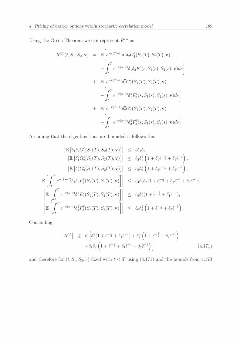
4 Pricing of barrier options within stochastic correlation model 189
Using the Green Theorem we can represent Rǫ,δ as
Rǫ,δ (t, S1, S2,v) = E
[
e−r(T−t)δ1δ2Gǫ1(S1(T ), S2(T ),v)
−∫ T
t
e−r(s−t)δ1δ2Fǫ1(s, S1(s), S2(s),v)ds
]
+ E
[
e−r(T−t)δ21Gǫ2(S1(T ), S2(T ),v)
−∫ T
t
e−r(s−t)δ21Fǫ2(s, S1(s), S2(s),v)ds
]
+ E
[
e−r(T−t)δ22Gǫ3(S1(T ), S2(T ),v)
−∫ T
t
e−r(s−t)δ22Fǫ3(s, S1(s), S2(s),v)ds
]
.
Assuming that the eigenfunctions are bounded it follows that
∣∣E[δ1δ2G
ǫ1(S1(T ), S2(T ),v)
]∣∣ ≤ cδ1δ2,
∣∣E[δ21G
ǫ2(S1(T ), S2(T ),v)
]∣∣ ≤ c2δ
21
(
1 + δ1ǫ− 1
2 + δ1ǫ−1)
,
∣∣E[δ22G
ǫ3(S1(T ), S2(T ),v)
]∣∣ ≤ c3δ
22
(
1 + δ2ǫ− 1
2 + δ2ǫ−1)
,∣∣∣∣E
[∫ T
t
e−r(s−t)δ1δ2Fǫ1(S1(T ), S2(T ),v)
]∣∣∣∣≤ c4δ1δ2(1 + ǫ−
12 + δ1ǫ
−1 + δ2ǫ−1),
∣∣∣∣E
[∫ T
t
e−r(s−t)δ21Fǫ2(S1(T ), S2(T ),v)
]∣∣∣∣≤ c5δ
21(1 + ǫ−
12 + δ1ǫ
−1),
∣∣∣∣E
[∫ T
t
e−r(s−t)δ22Fǫ3(S1(T ), S2(T ),v)
]∣∣∣∣≤ c6δ
22
(
1 + ǫ−12 + δ2ǫ
−1)
.
Concluding,
∣∣Rǫ,δ
∣∣ ≤ c7
[
δ21(1 + ǫ−12 + δ1ǫ
−1) + δ22
(
1 + ǫ−12 + δ2ǫ
−1)
+δ1δ2
(
1 + ǫ−12 + δ1ǫ
−1 + δ2ǫ−1) ]
, (4.171)
and therefore for (t, S1, S2, v) fixed with t < T using (4.171) and the bounds from 4.170
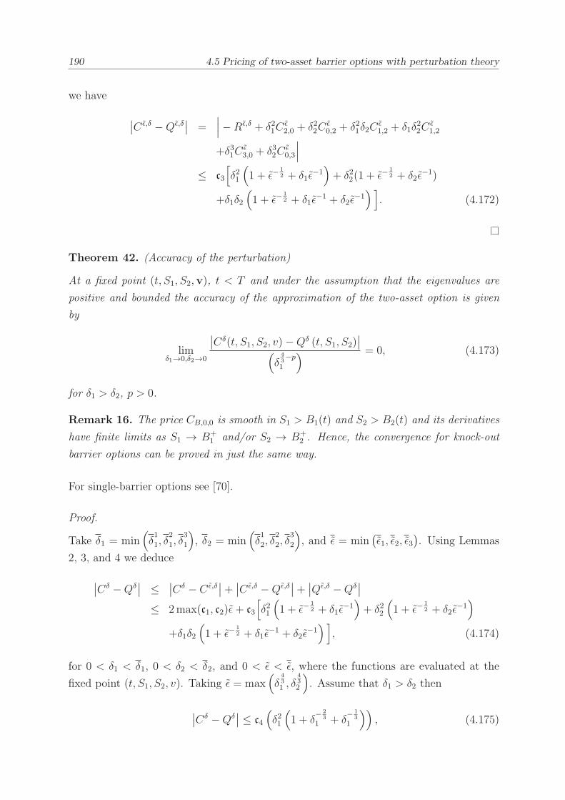
190 4.5 Pricing of two-asset barrier options with perturbation theory
we have
∣∣C ǫ,δ −Qǫ,δ
∣∣ =
∣∣∣−Rǫ,δ + δ21C
ǫ2,0 + δ22C
ǫ0,2 + δ21δ2C
ǫ1,2 + δ1δ
22C
ǫ1,2
+δ31Cǫ3,0 + δ32C
ǫ0,3
∣∣∣
≤ c3
[
δ21
(
1 + ǫ−12 + δ1ǫ
−1)
+ δ22(1 + ǫ−12 + δ2ǫ
−1)
+δ1δ2
(
1 + ǫ−12 + δ1ǫ
−1 + δ2ǫ−1) ]
. (4.172)
Theorem 42. (Accuracy of the perturbation)
At a fixed point (t, S1, S2,v), t < T and under the assumption that the eigenvalues are
positive and bounded the accuracy of the approximation of the two-asset option is given
by
limδ1→0,δ2→0
∣∣Cδ(t, S1, S2, v)−Qδ (t, S1, S2)
∣∣
(
δ43−p
1
) = 0, (4.173)
for δ1 > δ2, p > 0.
Remark 16. The price CB,0,0 is smooth in S1 > B1(t) and S2 > B2(t) and its derivatives
have finite limits as S1 → B+1 and/or S2 → B+
2 . Hence, the convergence for knock-out
barrier options can be proved in just the same way.
For single-barrier options see [70].
Proof.
Take δ1 = min(
δ1
1, δ2
1, δ3
1
)
, δ2 = min(
δ1
2, δ2
2, δ3
2
)
, and ǫ = min(ǫ1, ǫ2, ǫ3
). Using Lemmas
2, 3, and 4 we deduce
∣∣Cδ −Qδ
∣∣ ≤
∣∣Cδ − C ǫ,δ
∣∣+∣∣C ǫ,δ −Qǫ,δ
∣∣+∣∣Qǫ,δ −Qδ
∣∣
≤ 2max(c1, c2)ǫ+ c3
[
δ21
(
1 + ǫ−12 + δ1ǫ
−1)
+ δ22
(
1 + ǫ−12 + δ2ǫ
−1)
+δ1δ2
(
1 + ǫ−12 + δ1ǫ
−1 + δ2ǫ−1) ]
, (4.174)
for 0 < δ1 < δ1, 0 < δ2 < δ2, and 0 < ǫ < ǫ, where the functions are evaluated at the
fixed point (t, S1, S2, v). Taking ǫ = max(
δ431 , δ
432
)
. Assume that δ1 > δ2 then
∣∣Cδ −Qδ
∣∣ ≤ c4
(
δ21
(
1 + δ− 2
31 + δ
− 13
1
))
, (4.175)
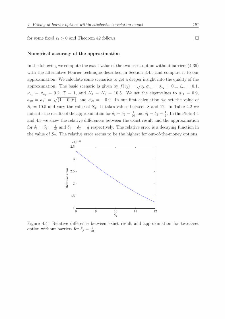
4 Pricing of barrier options within stochastic correlation model 191
for some fixed c4 > 0 and Theorem 42 follows.
Numerical accuracy of the approximation
In the following we compute the exact value of the two-asset option without barriers (4.36)
with the alternative Fourier technique described in Section 3.4.5 and compare it to our
approximation. We calculate some scenarios to get a deeper insight into the quality of the
approximation. The basic scenario is given by f(vj) =√vj, σv1 = σv2 = 0.1, ζvj = 0.1,
κv1 = κv2 = 0.2, T = 1, and K1 = K2 = 10.5. We set the eigenvalues to a11 = 0.9,
a12 = a21 =√
(1− 0.92), and a22 = −0.9. In our first calculation we set the value of
S1 = 10.5 and vary the value of S2. It takes values between 8 and 12. In Table 4.2 we
indicate the results of the approximation for δ1 = δ2 =120
and δ1 = δ2 =12. In the Plots 4.4
and 4.5 we show the relative differences between the exact result and the approximation
for δ1 = δ2 =120
and δ1 = δ2 =12respectively. The relative error is a decaying function in
the value of S2. The relative error seems to be the highest for out-of-the-money options.
Relativeerror
S2
8 9 10 11 12
×10−3
1
1.5
2
2.5
3
3.5
Figure 4.4: Relative difference between exact result and approximation for two-assetoption without barriers for δj =
120.
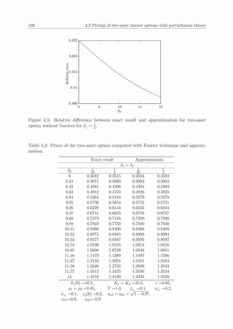
192 4.5 Pricing of two-asset barrier options with perturbation theory
Relativeerror
S2
8 9 10 11 120, 006
0, 01
0, 014
0.018
0, 022
Figure 4.5: Relative difference between exact result and approximation for two-assetoption without barriers for δj =
12.
Table 4.2: Prices of the two-asset option computed with Fourier technique and approxi-mation.
Exact result Approximation
δ1 = δ2S2
120
12
120
12
8 0.3582 0.3515 0.3594 0.35928,21 0.3971 0.3900 0.3983 0.39828,42 0.4381 0.4306 0.4394 0.43938,63 0.4812 0.4734 0.4826 0.48258,84 0.5264 0.5184 0.5279 0.52789,05 0.5736 0.5654 0.5752 0.57519,26 0.6229 0.6144 0.6245 0.62449,47 0.6741 0.6655 0.6758 0.67579,68 0.7273 0.7185 0.7289 0.72909,89 0.7822 0.7733 0.7840 0.784010,11 0.8390 0.8300 0.8408 0.840910,32 0.8975 0.8885 0.8993 0.899410,53 0.9577 0.9487 0.9595 0.959710,74 1.0196 1.0105 1.0214 1.021610,95 1.0830 1.0739 1.0848 1.085111,16 1.1479 1.1389 1.1497 1.150011,37 1.2143 1.2054 1.2161 1.216411,58 1.2820 1.2732 1.2838 1.284311,75 1.3512 1.3425 1.3530 1.353412 1.4216 1.4130 1.4234 1.4239
S1(0) =10.5, K1 = K2 =10.5, r =0.05,ρ1 = ρ2 =0.05, T =1.0, ζvj =0.1, κvj =0.2,
σvj =0.1, vj(0) =0.2, a12 = a21 =√1− 0.92,
a11=0.9, a22=-0.9
4 Pricing of barrier options within stochastic correlation model 193
4.5.2 Extension of Model (4.1)
We suggest here an extension to Model (4.1) and introduce – beside the fast mean-
reverting component – a further, slow mean-reverting component to the stochastic dy-
namic of the eigenvalue. In this context we shortly want to give an insight how per-
turbation could be applied in the extended model as well. Further future research will
have to be undertaken as far as for example convergence and the number of necessary
perturbation terms are concerned. The following model is suggested:
dSi = rSidt+ Si
p∑
j=1
aijf(vj(t), yj(t))dWj, i ∈ 1, 2 , p = 2 (4.176)
dvj =κvjδ2j
(ζvj − vj)dt+σvjδj
√vjdZvj , (4.177)
dyj = ǫ2jκyj(ζyj − yj)dt+ ǫjσyj√yjdZyj , (4.178)
⟨dWj, dZvj
⟩= ρvjdt,
⟨dWj, dZyj
⟩= ρyjdt,
⟨dZvj , dZyj
⟩= ρvyj dt, for j ∈ 1, 2 ,
all other correlations are set to 0. To allow for slow mean reversion we assume ǫj very
small.
In the following we shortly indicate how an approximation applying perturbation theory
could by analogously to before performed in this model.13
As before we price in this framework options which depend on two underlyings with and
without barriers on both of the underlyings (see (4.36) and (4.37)). The payoff in T is
indicated by g(S1, S2) in the following. We asymptotically approximate the prices with
singular (in δj) and regular (in ǫj) perturbation theory. The infinitesimal generator Lδ,ǫ
is again expressed as a power series, this time in ǫj and δj
Lδ1,δ2,ǫ1,ǫ2 =1
δ21L1
0 +1
δ22L2
0 +1
δ1L1
1 +1
δ2L2
1 + L2 + ε21M10 + ε22M2
0
+ε1M11 + ε2M2
1 +ε1δ1M1
3 +ε2δ2M2
3, (4.179)
13This chapter has been prepared during a master thesis project in cooperation with Daniela Neykova.See also [90]
194 4.5 Pricing of two-asset barrier options with perturbation theory
where
L10 = κv1(ζv1 − v1)
∂
∂v1+
1
2σ2v1v1∂2
∂v21, (4.180)
L20 = κv2(ζv2 − v2)
∂
∂v2+
1
2σ2v2v2∂2
∂v22, (4.181)
L11 = ρv1a11f1(v1, y1)σv1
√v1S1
∂2
∂S1∂v1+ ρv1a21f1(v1, y1)σv1
√v1S2
∂2
∂S2∂v1, (4.182)
L21 = ρv2a12f2(v2, y2)σv2
√v2S1
∂2
∂S1∂v2+ ρv2a22f2(v2, y2)σv2
√v2S2
∂2
∂S2∂v2, (4.183)
L2 =∂
∂t+ r
(
S1∂
∂S1
+ S2∂
∂S2
− ·)
+(a11a21f
21 + a12a22f
22
)S1S2
∂2
∂S1∂S2
+1
2
(a211f
21 + a212f
22
)S21
∂2
∂S21
+1
2
(a221f
21 + a222f
22
)S22
∂2
∂S22
, (4.184)
M10 = κy1(ζy1 − y1)
∂
∂y1+
1
2σ2y1y1∂2
∂y21, (4.185)
M20 = κy2(ζy2 − y2)
∂
∂y2+
1
2σ2y2y2∂2
∂y22, (4.186)
M11 = ρy1a11f1σy1
√y1S1
∂2
∂S1∂y1+ ρy1a21f1σy1
√y1S2
∂2
∂S2∂y1, (4.187)
M21 = ρy2a12f2σy2
√y2S1
∂2
∂S1∂y2+ ρy2a22f2σy2
√y2S2
∂2
∂S2∂y2, (4.188)
M13 = ρvy1 σv1σy1
√v1y1
∂2
∂v1∂y1, (4.189)
M23 = ρvy2 σv2σy2
√v2y2
∂2
∂v2∂y2, (4.190)
where fj = (vj, yj). The problem to be solved for the two-asset option Cδ,ǫ, hence, becomes
Lδ,ǫCδ,ǫ = 0, (4.191)
Cδ,ǫ(T, S1, S2) = g(S1, S2),
and for the barrier option, respectively,
LδCδ,ǫB = 0,
Cδ,ǫB (t, B1(t), S2) = 0,
Cδ,ǫB (t, S1, B2(t)) = 0,
Cδ,ǫB (T, S1, S2) = g(S1, S2). (4.192)
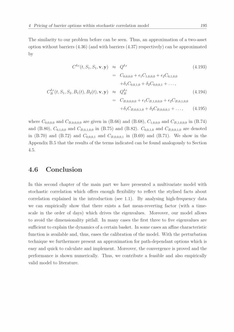
4 Pricing of barrier options within stochastic correlation model 195
The similarity to our problem before can be seen. Thus, an approximation of a two-asset
option without barriers (4.36) (and with barriers (4.37) respectively) can be approximated
by
Cδ,ǫ(t, S1, S1,v,y) ≈ Qδ,ǫ (4.193)
= C0,0,0,0 + ǫ1C1,0,0,0 + ǫ2C0,1,0,0
+δ1C0,0,1,0 + δ2C0,0,0,1 + . . . ,
Cδ,ǫB (t, S1, S2, B1(t), B2(t),v,y) ≈ Qδ,ǫ
B (4.194)
= CB,0,0,0,0 + ǫ1CB,1,0,0,0 + ǫ2CB,0,1,0,0
+δ1CB,0,0,1,0 + δ2CB,0,0,0,1 + . . . , (4.195)
where C0,0,0,0 and CB,0,0,0,0 are given in (B.66) and (B.68), C1,0,0,0 and CB,1,0,0,0 in (B.74)
and (B.80), C0,1,0,0 and CB,0,1,0,0 in (B.75) and (B.82). C0,0,1,0 and CB,0,0,1,0 are denoted
in (B.70) and (B.72) and C0,0,0,1 and CB,0,0,0,1 in (B.69) and (B.71). We show in the
Appendix B.5 that the results of the terms indicated can be found analogously to Section
4.5.
4.6 Conclusion
In this second chapter of the main part we have presented a multivariate model with
stochastic correlation which offers enough flexibility to reflect the stylised facts about
correlation explained in the introduction (see 1.1). By analysing high-frequency data
we can empirically show that there exists a fast mean-reverting factor (with a time-
scale in the order of days) which drives the eigenvalues. Moreover, our model allows
to avoid the dimensionality pitfall. In many cases the first three to five eigenvalues are
sufficient to explain the dynamics of a certain basket. In some cases an affine characteristic
function is available and, thus, eases the calibration of the model. With the perturbation
technique we furthermore present an approximation for path-dependant options which is
easy and quick to calculate and implement. Moreover, the convergence is proved and the
performance is shown numerically. Thus, we contribute a feasible and also empirically
valid model to literature.


Part III
Appendix

Appendix A
Appendix for Chapter 3
A.1 Appendix for Section 3.4
A.1.1 Transformations used for PDE
For constant barriers B1 and B2 (only GBM framework):
12σ21S
21∂2C∂S2
1+ 1
2σ22S
22∂2C∂S2
2+ ρσ1σ2S1S2
∂2C∂S1∂S2
+
+rS1∂C∂S1
+ rS2∂C∂S2
+ ∂C∂t− rC = 0,
C(t, B1, S2) = 0, C(t, S1, B2) = 0,
C(T, S1, S2, B1, B2) = g (S1, S2)1ιt>T,ι2>T.
(A.1)
Transform Si to xi := ln( Si
Ki) and Bi to bi := ln(Bi
Ki). The new derivatives in terms of C ′
are given by
∂C
∂Si
=1
Si
∂C ′
∂xi,
∂2C
∂S2i
=1
S2i
∂2C ′
∂x2i− 1
S2i
∂C ′
∂xi,
∂2C
∂SiSj
=1
SiSj
∂2C ′
∂xi∂xj.

200 A.1 Appendix for Section 3.4
Thus, the PDE in terms of C ′(t, x1, x2, b1, b2) has the form
12σ21∂2C′
∂x21+ 1
2σ22∂2C′
∂x22+ (r − 1
2σ21)
∂C′
∂x1+ (r − 1
2σ22)
∂C′
∂x2+ ρσ1σ2
∂2C′
∂x1∂x2+
+∂C′
∂t− rC ′ = 0,
C ′ (t, b1, x2) = 0, C ′ (t, x1, b2) = 0,
C ′ (T, x1, x2, b1, b2) = g (x1, x2)1ι1>T,ι2>T.
(A.2)
Then transform to G := e∫ Tt
r(s)ds−β1x1−β2x2+α(T−t)C ′. The derivatives are given by
∂C ′
∂t= e−
∫ Tt
r(s)ds+β1x1+β2x2+αt
(
(r + α)G+∂G
∂t
)
,
∂C ′
∂xi= e−
∫ Tt
r(s)ds+β1x1+β2x2+αt
(
βiG+∂G
∂xi
)
,
∂2C ′
∂x2i= e−
∫ Tt
r(s)ds+β1x1+β2x2+αt
(
2βi∂G
∂xi+ β2
iG+∂2G
∂x2i
)
,
∂2C
∂xi∂xj= e−
∫ Tt
r(s)ds+β1x1+β2x2+αt
(
βiβjG+ βj∂G
∂xi+ βi
∂G
∂xj
)
.
β1 and β2 are determined in such a way that we get rid of the first derivatives in x1 and
x2. Thus,
β1 =σ1
(12− r
σ21
)
− ρσ2(12 − rσ22)
σ1 (1− ρ2),
β2 =σ2(
12− r
σ22)− ρσ1
(12− r
σ21
)
σ2 (1− ρ2),
α = −1
2σ21β
21 −
1
2σ22β
22 − (r − 1
2σ21)β
21 − (r − 1
2σ22)β
22 − ρσ1σ2β1β2.
Inserting βi and α and grouping the derivatives of order one and the terms in G this
becomes clear
∂G
∂x1
(
−1
2σ21 + σ2
1β1 + ρσ1σ2β2 + r
)
=∂G
∂x1
−1
2σ21 + σ2
1
σ1
(12− r
σ21
)
− ρσ2(12 − rσ22)
σ1 (1− ρ2)+ ρσ1σ2
σ2(12− r
σ22)− ρσ1
(12− r
σ21
)
σ2 (1− ρ2)+ r
=∂G
∂x1
−1
2σ21 (1− ρ2)
(1− ρ2) +σ21
(12− r
σ21
)
− ρ2σ21
(12− r
σ21
)
(1− ρ2) +r (1− ρ2)(1− ρ2)
= 0.
A Appendix for Chapter 3 201
The same is true for ∂G∂t.
G
(
−r + r + α + (r − 1
2σ21)β1 + (r − 1
2σ22)β2 + ρσ1σ2β1β2 +
1
2σ21β
21 +
1
2σ22β2
2
)
= 0.
(A.3)
The PDE for G(t, x1, x2, b1, b2) is given by
12σ21∂2G∂x2
1+ 1
2σ22∂2G∂x2
2+ ρσ1σ2
∂2G∂x1∂x2
++∂G∂t
= 0,
G (t, b1, x2) = 0, G (t, x1, b2) = 0,
G (T, x1, x2, b1, b2) = g (x1, x2)1ι1>T,ι2>Te−β1x1−β2x2 .
(A.4)
The respective Kolmogorov backward equation for the transition density p(t, x′1, x′2, x1, x2)
is now given by (see Remark 7)
− ∂p
∂t=
1
2σ21
∂2p
∂x21+
1
2σ22
∂2p
∂x22+ ρσ1σ2
∂2p
∂x1∂x2(A.5)
p (t, x′1, x′2, b1, x2) = 0,
p (t, x′1, x′2, x1, b2) = 0,
p (T, x′1, x′2, x1, x2) = δ(x′1 − x1)δ(x′2 − x2). (A.6)
This equation can be transformed in the standard form by the transformation τ := T − t:
∂p
∂τ=
1
2σ21
∂2p
∂x21+
1
2σ22
∂2p
∂x22+ ρσ1σ2
∂2p
∂x1∂x2(A.7)
p (τ, x′1, x′2, x
′1, x
′2, b1, x2) = 0,
p (τ, x′1, x′2, x1, b2) = 0,
p (0, x′1, x′2, x1, x2) = δ(x′1 − x1)δ(x′2 − x2). (A.8)
By Fourier transforming this PDE we find that the equation the characteristic function
ϕ has to fulfil. We set ϕ(τ, u1, u2, x′1, x
′2) :=
∫∞−∞∫∞−∞ ei(u1x1+u2x2)p(τ, x′1, x
′2, x1, x2)dx1dx2
or respectively p(τ, x′1, x′2, x1, x2) := 1
(2π)2
∫∞−∞∫∞−∞ e−i(u1x1+u2x2)ϕ(τ, u1, u2, x
′1, x
′2)du1du2.
202 A.1 Appendix for Section 3.4
Thus,
∂p
∂τ=
1
(2π)2
∫ ∞
−∞
∫ ∞
−∞e−i(u1x1+u2x2)
∂ϕ(τ, u1, u2, x′1, x
′2)
∂τdu1du2,
∂p
∂x1=
1
(2π)2
∫ ∞
−∞
∫ ∞
−∞−e−i(u1x1+u2x2)iu1ϕ(τ, u1, u2, x
′1, x
′2)du1du2,
∂2p
∂x21=
1
(2π)2
∫ ∞
−∞
∫ ∞
−∞−e−i(u1x1+u2x2)u21ϕ(τ, u1, u2, x
′1, x
′2)du1du2,
∂2p
∂x1∂x2=
1
(2π)2
∫ ∞
−∞
∫ ∞
−∞−e−i(u1x1+u2x2)u1u2ϕ(τ, u1, u2, x
′1, x
′2)du1du2,
ϕ(0, u1, u2, x′1, x
′2) =
∫ ∞
−∞
∫ ∞
−∞ei(u1x1+u2x2)δ(x′1 − x1)δ(x′2 − x2)dx1dx2
= ei(u1x′1+u2xz
′2)
and
∂ϕ
∂τ= −1
2σ21u
21ϕ−
1
2σ22u
22ϕ− ρσ1σ2u1u2ϕ (A.9)
ϕ (τ, u1, u2, b1, x′2) = 0,
ϕ (τ, u1, u2, x′1, b2) = 0,
ϕ (0, u1, u2, x′1, x
′2) = ei(u1x
′1+u2xz
′2). (A.10)
For time-dependent barriers, which are applied particularly in the case of stochastic or
local volatilities:
12v2νσ2
1S21∂2C∂S2
1+ 1
2v2νσ2
2S22∂2C∂S2
2+ ρv2νσ1σ2S1S2
∂2C∂S1∂S2
+
12ǫ2v2γ ∂2C
∂v2+ rS1
∂C∂S1
+ rS2∂C∂S2
+ κ(ζ − v)∂C∂v
+ ∂C∂t− rC = 0,
C (t, B1(t), S2) = 0, C (t, S1, B2(t)) = 0,
C (T, S1, S2, B1(t), B2(t)) = g (S1, S2)1ι1>T,ι2>T.
(A.11)
To reduce the above PDE transform Si to xi := ln(Sie∫Tt r(s)ds
Ki) and Bi(t) to bi :=
ln(
Bi(T )Ki
)
for i ∈ 1, 2. The new derivatives for C(t, S1, S2, K1, K2, B1(t), B2(t)) in

A Appendix for Chapter 3 203
terms of C ′(t, x1, x2, B1(t), B2(t)) are given by
∂C
∂t=
∂C ′
∂t− r
2∑
i=1
∂C ′
∂xi,
∂C
∂Si
=1
Si
∂C ′
∂xi,
∂2C
∂S2i
=1
S2i
∂2C ′
∂x2i− 1
S2i
∂C ′
∂xi,
∂2C
∂SiSj
=1
SiSj
∂2C ′
∂xi∂xj.
Thus, the PDE in terms of C ′(t, x1, x2, b1, b2) has the form
12v2νσ2
1∂2C′
∂x21+ 1
2v2νσ2
2∂2C′
∂x22− 1
2v2νσ2
1∂C′
∂x1− 1
2v2νσ2
2∂C′
∂x2+ ρv2νσ1σ2
∂C′
∂x1∂x2+
12ǫ2v2γ ∂2C′
∂v2+ κ(ζ − v)∂C′
∂v+ ∂C′
∂t− rC ′ = 0,
C ′ (t, b1, x2) = 0, C ′ (t, x1, b2) = 0,
C ′ (T, x1, x2, b1, b2) = g (x1, x2)1ι1>T,ι2>T.
(A.12)
Then transform to G := e∫ Tt
r(s)ds−c1x1−c2x2C ′. The derivatives are given by
∂C ′
∂t= e−
∫ Tt
r(s)ds+c1x1+c2x2
(
rG+∂G
∂t
)
,
∂C ′
∂xi= e−
∫ Tt
r(s)ds+c1x1+c2x2
(
ciG+∂G
∂xi
)
,
∂2C ′
∂x2i= e−
∫ Tt
r(s)ds+c1x1+c2x2
(
2ci∂G
∂xi+ c2iG+
∂2G
∂x2i
)
,
∂2C ′
∂xi∂xj= e−
∫ Tt
r(s)ds+c1x1+c2x2
(
cicjG+ cj∂G
∂xi+ ci
∂G
∂xj
)
.
c1 and c2 are determined in such a way that we get rid of the first derivatives in x1 and
x2:
c1 =σ1 − σ2ρ
2σ1 (1− ρ2),
c2 =σ2 − σ1ρ
2σ2 (1− ρ2).
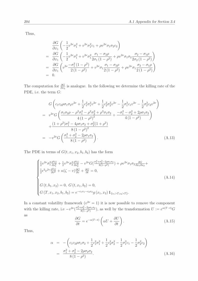
204 A.1 Appendix for Section 3.4
Thus,
∂G
∂x1
(
−1
2v2νσ2
1 + v2νσ21c1 + ρv2νσ1σ2c2
)
=∂G
∂x1
(
−1
2v2νσ2
1 + v2νσ21
σ1 − σ2ρ2σ1 (1− ρ2)
+ ρv2νσ1σ2σ2 − σ1ρ
2σ2 (1− ρ2)
)
=∂G
∂x1
(
v2ν−σ2
1 (1− ρ2)2 (1− ρ2) + v2νσ1
σ1 − σ2ρ2 (1− ρ2) + ρv2νσ1
σ2 − σ1ρ2 (1− ρ2)
)
= 0.
The computation for ∂G∂x2
is analogue. In the following we determine the killing rate of the
PDE, i.e. the term G:
G
(
c1c2ρσ1σ2v2ν +
1
2c21σ
21v
2ν +1
2c22σ
22v
2ν − 1
2σ21c1v
2ν − 1
2σ22c2v
2ν
)
= v2νG
(σ1σ2ρ− ρ2σ2
1 − ρ2σ22 + ρ3σ1σ2
4 (1− ρ2)2+−σ2
1 − σ22 + 2ρσ1σ2
4 (1− ρ2)
)
+(1 + ρ2)σ2
1 − 4ρσ1σ2 + σ22(1 + ρ2)
8 (1− ρ2)2
= −v2νG(σ21 + σ2
2 − 2ρσ1σ28 (1− ρ2)
)
. (A.13)
The PDE in terms of G(t, x1, x2, b1, b2) has the form
12v2νσ2
1∂2G∂x2
1+ 1
2v2νσ2
2∂2G∂x2
2− v2νG(σ2
1+σ22−2ρσ1σ2
8(1−ρ2)) + ρv2νσ1σ2
∂G∂x1∂x2
+
12ǫ2v2γ ∂2G
∂v2+ κ(ζ − v)∂G
∂v+ ∂G
∂t= 0,
G (t, b1, x2) = 0, G (t, x1, b2) = 0,
G (T, x1, x2, b1, b2) = e−c1x1−c2x2g (x1, x2)1ι1>T,ι2>T.
(A.14)
In a constant volatility framework (v2ν = 1) it is now possible to remove the component
with the killing rate, i.e −v2ν(σ21+σ2
2−2ρσ1σ2
8(1−ρ2)), as well by the transformation U := eα(T−t)G
as∂G
∂t= e−α(T−t)
(
αU +∂U
∂t
)
. (A.15)
Thus,
α = −(
c1c2ρσ1σ2 +1
2c21σ
21 +
1
2c22σ
22 −
1
2σ21c1 −
1
2σ22c2
)
=σ21 + σ2
2 − 2ρσ2σ28 (1− ρ2) . (A.16)

A Appendix for Chapter 3 205
By introducing
z1 :=1
√
1− ρ2
(x1σ1− ρx2
σ2
)
,
z2 :=x2σ2, (A.17)
the mixing derivative in x1 and x2 is removed. The derivatives are given by
∂
∂x1=
1√
1− ρ2σ1∂
∂z1,
∂
∂x2=
1
σ2
∂
∂z2− ρ√
1− ρ2σ2∂
∂z1,
∂2
∂x21=
1
(1− ρ2) σ21
∂2
∂z21,
∂2
∂x22=
1
σ22
∂2
∂z22+
ρ2
(1− ρ2) σ22
∂2
∂z21− 2
ρ√
1− ρ2σ22
∂2
∂z1∂z2,
∂2
∂x1∂x2= − ρ
(1− ρ2) σ1σ1∂2
∂z21+
1
σ1σ2√
1− ρ2∂2
∂z1∂z2.
We insert these derivatives and group terms of the same derivative:
∂2G
∂z21
(1
2v2νσ2
1 +1
2v2νσ2
2
ρ2
σ22 (1− ρ2)
− v2νσ1σ2ρρ
σ1σ2 (1− ρ2)
)
=1
2v2ν
∂2G
∂z21,
∂2G
∂z1∂z2
(
−212v2νσ2
2
ρ
σ22
√
1− ρ2+ v2νσ1σ2ρ
1
σ1σ2√
1− ρ2
)
= 0.
Furthermore, we transform t→ τ , where τ := T − t.
−12v2ν ∂2G
∂z21− 1
2v2ν ∂2G
∂z22+ v2νG(
σ21+σ2
2−2ρσ1σ2
8(1−ρ2))−
12ǫ2v2γ ∂2G
∂v2− κ(ζ − v)∂G
∂v+ ∂G
∂τ= 0,
G (τ, z1, 0) = 0, G
(
τ, z1,−√
1−ρ2
ρz1
)
= 0,
G (0, z1, z2) = e−c1x1−c2x2g (z1, z2)1ι1>T,ι2>T.
(A.18)
The respective Kolmogorov backward equation for the transition density

206 A.1 Appendix for Section 3.4
p(τ, z′1, z′2, z1, z2, v) is given by
∂p
∂τ=
1
2v2ν
∂2p
∂z21+
1
2v2ν
∂2p
∂z22− v2νp(σ
21 + σ2
2 − 2ρσ1σ28 (1− ρ2) )
+1
2ǫ2v2γ
∂2p
∂v2+ κ(ζ − v)∂p
∂v, (A.19)
p (τ, z′1, z′2, z1, 0) = 0,
p
(
τ, z′1, z′2, z1,−
√
1− ρ2ρ
z1
)
= 0,
p (0, z′1, z′2, z1, z2) = δ(z′1 − z1)δ(z′2 − z2). (A.20)
By Fourier transforming this PDE we find the equation the characteristic function ϕ has
to fulfil. We set ϕ(τ, u1, u2, z′1, z
′2) :=
∫∞−∞∫∞−∞ ei(u1z1+u2z2)p(τ, z′1, z
′2, z1, z2)dz1dz2 or re-
spectively p(τ, z′1, z′2, z1, z2) :=
1(2π)2
∫∞−∞∫∞−∞ e−i(u1x1+u2x2)ϕ(τ, u1, u2, z
′1, z
′2)du1du2. Thus,
∂p
∂τ=
1
(2π)2
∫ ∞
−∞
∫ ∞
−∞e−i(u1z1+u2z2)
∂ϕ(τ, u1, u2, z′1, z
′2)
∂τdu1du2,
∂p
∂z1=
1
(2π)2
∫ ∞
−∞
∫ ∞
−∞−e−i(u1z1+u2z2)iu1ϕ(τ, u1, u2, z
′1, z
′2)du1du2,
∂2p
∂z21=
1
(2π)2
∫ ∞
−∞
∫ ∞
−∞−e−i(u1z1+u2z2)u21ϕ(τ, u1, u2, z
′1, z
′2)du1du2,
∂p
∂v=
1
(2π)2
∫ ∞
−∞
∫ ∞
−∞e−i(u1z1+u2z2)
∂ϕ(τ, u1, u2, z′1, z
′2)
∂vdu1du2,
ϕ(0, u1, u2, z′1, z
′2)) =
∫ ∞
−∞
∫ ∞
−∞ei(u1z1+u2z2)δ(z′1 − z1)δ(z′2 − z2)dz1dz2
= ei(u1z′1+u2z
′2) (A.21)
and we get
∂ϕ
∂τ= −1
2v2νu21ϕ−
1
2v2νu22ϕ− v2νϕ(
σ21 + σ2
2 − 2ρσ1σ28 (1− ρ2) )
+1
2ǫ2v2γ
∂2ϕ
∂v2+ κ(ζ − v)∂ϕ
∂v, (A.22)
ϕ (τ, u1, u2, z′1, 0) = 0,
ϕ
(
τ, u1, u2, z′1,−
√
1− ρ2ρ
z′1
)
= 0,
ϕ (0, u1, u2, z′1, z
′2) = ei(u1z
′1+u2z
′2). (A.23)

A Appendix for Chapter 3 207
A.1.2 Characteristic functions
Proof. (Derivation of Heston-type characteristic function)
Assume the following affine form
ϕH(τ,u) = exp
iu1z1 + iu2z2 +1
σ2v
(AH(τ,u) + BH(τ,u)v)
, (A.24)
and plug it in the PDE (3.37) with ν = γ = 12:
1
σ2v
(∂AH(τ,u)
∂τ+ v
∂BH(τ,u)
∂τ
)
= −1
2v
(
u21 + u22 +σ21 + σ2
2 − 2ρσ1σ14(1− ρ2)
)
+1
2σ2v
vBH(τ,u)2 +
1
σ2v
κ(ζ − v)BH(τ,u),
AH(0,u) = 0, (A.25)
BH(0,u) = 0. (A.26)
We find then the following ODEs for AH and BH .
∂AH(τ,u)
∂τ− κζBH(τ,u) = 0,
AH(0,u) = 0, (A.27)
∂BH(τ,u)
∂τ− 1
2BH(τ,u)
2 + κBH(τ,u)
+1
2σ2v
(
u21 + u22 +σ21 + σ2
2 − 2ρσ1σ14(1− ρ2)
)
= 0,
BH(0,u) = 0. (A.28)
For the proof of the solution see Lipton (see [83], p. 380). (A.28) is a Riccati ODE which
we solve with the usual transformation BH = −2∂EH∂τ
EH. In terms of EH(τ,u), AH(τ,u)
can be written as AH = −2κζ lnEH . The ODE and appropriate initial conditions for
EH(τ,u) have the form
− 2∂2EH
∂τ2
EH
+ 2
(∂EH
∂τ
EH
)2
− 2
(∂EH
∂τ
EH
)2
−2κ∂EH
∂τ
EH
+1
2σ2v
(
u21 + u22 +σ21 + σ2
2 − 2ρσ1σ24(1− ρ2)
)
= 0,
⇔ ∂2EH
∂τ 2+ κ
∂EH
∂τ− 1
4σ2v
(
u12 + u22 +
σ21 + σ2
2 − 2ρσ1σ24(1− ρ2)
)
EH = 0,
EH(0,u) = 1,∂EH
∂τ(0,u) = 0. (A.29)

208 A.1 Appendix for Section 3.4
The general solution of (A.29) can be indicated by
EH(τ,u) = eH+eKH+τ + eH−e
KH−τ , (A.30)
where eH± are arbitrary constants and KH± solve the following quadratic equation
K2H± + κKH± −
1
4σ2v
(
u21 + u22 +σ21 + σ2
2 − 2ρσ1σ24(1− ρ2)
)
= 0. (A.31)
Hence,
KH± =
−κ±√
κ2 + σ2v
(
u21 + u22 +σ21+σ2
2−2ρσ1σ2
4(1−ρ2)
)
2. (A.32)
We introduce d = d(u) =
√
κ2 + σ2v
(
u21 + u22 +σ21+σ2
2−2ρσ1σ2
4(1−ρ2)
)
. EH(τ,u) has, thus, the
following form
EH(τ,u) = eH+e12(−κ+d)τ + eH−e
12(−κ−d)τ . (A.33)
From the first initial condition follows eH+ = 1 − eH−. From the second equation we
obtain for eH− = −κ+d2d
and for eH+ = κ+d2d
. Thus,
EH(τ,u) =(κ+ d)e
12(−κ+d)τ + (−κ+ d)e
12(−κ−d)τ
2d
= e12(−κ+d)τ κ+ d+ (−κ+ d)e−dτ
2d. (A.34)
AH and BH have then the following solutions:
BH(τ,u) =(κ− d)(1− exp (−dτ))
1− κ−dκ+d
exp (−dτ)
= κ− dsinh( d
2τ) + κ
dcosh( d
2τ)
cosh( d2τ) + κ
dsinh( d
2τ), (A.35)
AH(τ,u) = ζκ
(
(κ− d) τ − 2 ln
(
1− κ−dκ+d
exp (−dτ)1− κ−d
κ+d
))
= κζ
(
κτ − 2 ln
(κ
dsinh
(d
2τ
)
+ cosh
(d
2τ
)))
. (A.36)

A Appendix for Chapter 3 209
Proof. (Derivation of Stein and Stein-type characteristic function)
For the Stein model we guess the following affine form.
ϕS2(τ,u) = exp
iu1z1 + iu2z2 +1
σ2v
(AS2(τ,u) + BS2(τ,u)v + CS2(τ,u)v
2)
, (A.37)
where AS2(0,u) = BS2(0,u) = CS2(0,u) = 0. We plug it in the PDE (3.37) with ν = 1
and γ = 0:
1
σ2v
(∂AS2(τ,u)
∂τ+ v
∂BS2(τ,u)
∂τ+ v2
∂CS2(τ,u)
∂τ
)
= −1
2v2(
u21 + u22 +σ21 + σ2
2 − 2ρσ1σ14(1− ρ2)
)
+1
2σ2v
( 1
σ4v
BS2(τ,u)2 +
4
σ4v
vBS2(τ,u)CS2(τ,u)
+2
σ2v
CS2(τ,u) +4
σ4v
v2CS2(τ,u)2)
+1
σ2v
κ(ζ − v) (B2S(τ,u) + 2vC2S(τ,u)) ,
AS2(0,u) = 0, (A.38)
BS2(0,u) = 0, (A.39)
CS2(0,u) = 0. (A.40)
Inserting (A.37) in (3.32) we find the following ODEs
∂AS2(τ,u)
∂τ− κζBS2(τ,u)− σ2
vCS2(τ,u)−1
2BS2(τ,u)
2 = 0,
AS2(0,u) = 0, (A.41)
∂BS2(τ,u)
∂τ+ κBS2(τ,u)− 2BS2(τ,u)CS2(τ,u)− 2κζCS2(τ,u) = 0,
BS2(0,u) = 0, (A.42)
∂CS2(τ,u)
∂τ+ 2κCS2(τ,u)− 2CS2(τ,u)
2
+σ2v
2
(
u21 + u22 +σ21 + σ2
2 − 2ρσ1σ24(1− ρ2)
)
= 0,
CS2(0,u) = 0. (A.43)
(A.43) is again a Riccati equation. We set CS2 = −12
∂DS2∂τ
DS2. The ODE and appropriate

210 A.1 Appendix for Section 3.4
initial conditions for DS2(τ,u) have the form:
− 1
2
∂2DS2
∂τ2
DS2
+1
2
(∂DS2
∂τ
DS2
)2
− 1
2
(∂DS2
∂τ
DS2
)2
− κ∂DS2
∂τ
DS2
+σ2v
2
(
u21 + u22 +σ21 + σ2
2 − 2ρσ1σ24(1− ρ2)
)
= 0,
∂2DS2
∂τ 2+ 2κ
∂DS2
∂τ− σ2
v
(
u21 + u22 +σ21 + σ2
2 − 2ρσ1σ24(1− ρ2)
)
DS2 = 0,
DS2(0,u) = 1,∂DS2
∂τ(0,u) = 0. (A.44)
The general solution of (A.44) can be indicated by
DS2(τ,u) = dS2+eLS2+τ + dS2−e
LS2−τ , (A.45)
where dS2± are arbitrary constants and LS2± solves the following quadratic equation
L2S2± + 2κLS2± − σ2
v
(
u21 + u22 +σ21 + σ2
2 − 2ρσ1σ24(1− ρ2)
)
= 0. (A.46)
Hence,
LS2± = −κ±√
κ2 + σ2v
(
u21 + u22 +σ21 + σ2
2 − 2ρσ1σ24(1− ρ2)
)
,
d = d(u) =
√
κ2 + σ2v
(
u21 + u22 +σ21 + σ2
2 − 2ρσ1σ24(1− ρ2)
)
.
DS2(τ,u) has, thus, the following form
DS2(τ,u) = dS2+e(−κ+d)τ + dS2−e
(−κ−d)τ . (A.47)
From the first initial condition follows dS2+ = 1 − dS2−. From the second equation we
obtain for dS2− = −κ+d2d
and for dS2+ = κ+d2d
.
DS2(τ,u) =(κ+ d)e(−κ+d)τ + (−κ+ d)e(−κ−d)τ
2d
=e−κτ
2d
(κ(edτ − e−dτ ) + d
(edτ + e−dτ
))
= e−κτ(κ
dsinh (dτ) + cosh (dτ)
)
.

A Appendix for Chapter 3 211
Similar to (A.35) we conclude
CS2(τ,u) =1
2
(
κ− dsinh (dτ) + κ
dcosh (dτ)
cosh (dτ) + κdsinh (dτ)
)
. (A.48)
(A.42) is a first-order ODE of the form dy
dτ+ p(τ)y = q(τ), which can be solved by
y =∫
exp(∫ τ ′
p(τ ′′)dτ ′′)q(τ ′)dτ ′+c
exp(∫ τ
p(τ ′)dτ ′). In this case p(τ) = κ − 2CS2(τ,u) and q(τ) = 2κζCS2(τ,u)
(see Arfken [7], p. 465ff). Due to the initial condition BS2 has the form
BS2(τ,u) =
(∫ τ
0
2κζCS2(τ′,u) exp
∫ τ ′
0
(κ− 2CS2(τ′′,u)dτ ′′)
dτ ′
)
exp
−∫ τ
0
κ− 2CS2(τ′,u)dτ ′
=
(∫ τ
0
2κζCS2(τ′,u) exp κτ ′ + ln (DS2(τ
′,u)) dτ ′)
exp −κτ − ln (DS2(τ,u))
=
(
−∫ τ
0
κζ∂DS2(τ
′,u)
∂τ ′exp(κτ ′)dτ ′
)1
DS2(τ,u)exp −κτ
= −κζ∫ τ
0
(
− κ(κ
dsinh(dτ ′) + cosh(dτ ′)
)
+d(κ
dcosh(dτ ′) + sinh(dτ ′)
))
dτ ′1
DS2(τ,u)exp −κτ
= −κζ exp −κτDS2(τ,u)
∫ τ
0
(d− κ2
d) sinh(dτ ′)dτ ′
=κζ exp −κτDS2(τ,u)
(
(1− κ2
d2) cosh(0)− (1− κ2
d2) cosh(dτ)
)
=κζ exp −κτDS2(τ,u)
((κ2
d2− 1
)
cosh (dτ)−(κ2
d2− 1
))
=1
d
((
κζd− κ3ζ
d
)
+ κ2ζ(κdcosh (dτ) + sinh (dτ)
)
cosh (dτ) + κdsinh (dτ)
−κζd(κdsinh (dτ) + cosh (dτ)
)
cosh (dτ) + κdsinh (dτ)
)
=1
d
(
κζd− κ3ζ
d
)
+ κ2ζ(sinh (dτ) + κ
dcosh (dτ)
)
cosh (dτ) + κdsinh (dτ)
− κζd
.

212 A.1 Appendix for Section 3.4
For AS2 we show that
AS2(τ,u) = −σ2v
2ln(
cosh (dτ) +κ
dsinh (dτ)
)
+σ2v
2κτ
+κ2ζ2d2 − κ4ζ2
2d3
(sinh (dτ)
cosh (dτ) + κdsinh (dτ)
− dτ
)
+κ2ζ(κζd− κ3ζ
d)
d3
(cosh (dτ)− 1
cosh (dτ) + κdsinh (dτ)
)
fulfils (A.41). For that reason we compute κζBS2 +12B2
S2:
κζBS2 +1
2B2
S2 =12κ2ζ2 + κ6ζ2
2d4− κ4ζ2
d2(cosh (dτ) + κ
dsinh (dτ)
)2
+κ2ζ
d2(κζd− κ3ζ
d)(sinh (dτ) + κ
dcosh (dτ)
)
(cosh (dτ) + κ
dsinh (dτ)
)2
+12κ4ζ2
d2
(sinh (dτ) + κ
dcosh (dτ)
)2
(cosh (dτ) + κ
dsinh (dτ)
)2 − 1
2κ2ζ2. (A.49)
This is compared to
∂AS2(τ,u)
∂τ=
σ2v
2
(
κ− dsinh (dτ) + κ
dcosh(dτ)
cosh (dτ) + κdsinh (dτ)
)
+
(cosh2(dτ)d− sinh2(dτ)d
(cosh (dτ) + κdsinh (dτ))2
− d
)(κ2ζ2
2d− κ4ζ2
2d3
)
+
(κ sinh2(dτ)− κ cosh2(dτ) + d sinh (dτ) + κ cosh (dτ)
(cosh (dτ) + κdsinh (dτ))2
)
·κ2ζ(κζ
d2− κ3ζ
d4
)
= σ2vCS2(τ,u) +
12κ2ζ2 − κ4ζ2
2d2− κ4ζ2
d2+ κ6ζ2
d4(cosh (dτ) + κ
dsinh (dτ)
)2
−1
2κ2ζ2 +
κ4ζ2
2d2+ κ2ζ(
κζ
d2− κ3ζ2
d4)d
sinh (dτ) + κdcosh (dτ)
(cosh (dτ) + κ
dsinh (dτ)
)2

A Appendix for Chapter 3 213
= σ2vCS2(τ,u) +
12κ2ζ2 − κ4ζ2
d2+ κ6ζ2
2d4(cosh (dτ) + κ
dsinh (dτ)
)2 −κ2ζ2
2
+
κ2ζ
d2
(
κζd− κ3ζ
d
) (sinh (dτ) + κ
dcosh (dτ)
)
(cosh (dτ) + κ
dsinh (dτ)
)2
+κ4ζ2
2d2
(cosh (dτ) + κ
dsinh (dτ)
)2
(cosh (dτ) + κ
dsinh (dτ)
)2
+κ4ζ2
2d2
(sinh2(dτ)− cosh2(dτ)
)
(cosh (dτ) + κ
dsinh (dτ)
)2 +κ6ζ2
2d4
(− sinh2(dτ) + cosh2(dτ)
)
(cosh (dτ) + κ
dsinh (dτ)
)2
= σ2vCS2(τ,u) + κζBS2(τ,u) +
1
2BS2(τ,u)
2. (A.50)
A.1.3 Method of images in a half-space
For the Corollaries 5 and 7 we apply the method of images in a half-space to the charac-
teristic function ϕ. Thus, according to (3.32) q(τ, z1, z2, v) satisfies the following PDE
∂q
∂τ=
1
2v2ν
∂2q
∂z21+
1
2v2ν
∂2q
∂z22− v2ν σ
21 + σ2
2 − 2ρσ1σ28(1− ρ2) q
+1
2σ2vv
2γ ∂2q
∂v2+ κ(ζ − v)∂q
∂v, (A.51)
with the following initial and boundary conditions
q(0, z1, z2, v) = δ(z′1 − z1)δ(z′2 − z2), (A.52)
q(τ, z1, 0, v) = 0. (A.53)
As before the idea is to find a solution GF for (A.51) and (A.52) in the whole plane first
and restrict it to the actual space (A.53) by the following approach G = GF + GG.
GF has been found in (3.35). GG must satisfy (A.51) and, as G is required to vanish at
z2 = 0, then GF = −GG in z2 = 0. Due to the form of GF we test for GG(τ, u1, u2, z′1 −
z1, z′2− z2) = −GF (τ, u1, u2, z
′1− z1, z′2+ z2). It can be easily seen that GG satisfies (A.51)
as there are only pure second order derivatives in zi. On the boundary GG is given by
GG(τ, z′1, z′2, v; z1, z2) =
1
4π2
∫ i2+∞
i2−∞
∫ i1+∞
i1−∞exp iu1(z′1 − z1) + iu2z2
+V (τ,u) du1du2 (A.54)

214 A.1 Appendix for Section 3.4
As V (τ,u) is symmetric in u2 (see (3.36)) GG is invariant to a reflection −u2 → u2 and,
thus, also to a reflection −z2 → z2. Hence GG = −GF at the boundary z2 = 0. In
the bounded area, i.e. for z2 > 0 the initial condition is satisfied as GF fulfils it. The
transition density function is therefore given by
q(τ, z′1, z′2, v; z1, z2) =
1
4π2
∫ i2+∞
i2−∞
∫ i1+∞
i1−∞
(
G(τ, u1, u2, z′1 − z1, z′2 − z2)
−G(τ, u1, u2, z′1 − z1, z′2 + z2)
)
du1du2,
u = w + i ∈ Sϕ. (A.55)
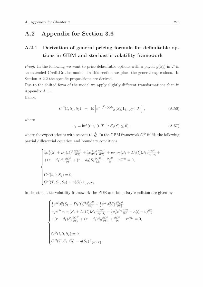
A Appendix for Chapter 3 215
A.2 Appendix for Section 3.6
A.2.1 Derivation of general pricing formula for defaultable op-
tions in GBM and stochastic volatility framework
Proof. In the following we want to price defaultable options with a payoff g(S2) in T in
an extended CreditGrades model. In this section we place the general expressions. In
Section A.2.2 the specific propositions are derived.
Due to the shifted form of the model we apply slightly different transformations than in
Appendix A.1.1.
Hence,
CD(t, S1, S2) = E
[
e−∫ Tt
r(s)dsg(S2)1ι1>T |Ft
]
, (A.56)
where
ι1 = inf (t′ ∈ (t, T ] : S1(t′) ≤ 0) , (A.57)
where the expectation is with respect to Q. In the GBM framework CD fulfils the following
partial differential equation and boundary conditions
12σ21(S1 +D1(t))
2 ∂2CD
∂S21
+ 12σ22S
22∂2CD
∂S22
+ ρσ1σ2(S1 +D1(t))S2∂2CD
∂S1∂S2+
+(r − d1)S1∂CD
∂S1+ (r − d2)S2
∂CD
∂S2+ ∂CD
∂t− rCD = 0,
CD(t, 0, S2) = 0,
CD(T, S1, S2) = g(S2)1ι1>T.
In the stochastic volatility framework the PDE and boundary condition are given by
12v2νσ2
1(S1 +D1(t))2 ∂2CD
∂S21
+ 12v2νσ2
2S22∂2CD
∂S22
+ρv2νσ1σ2(S1 +D1(t))S2∂2CD
∂S1∂S2+ 1
2σ2vv
2γ ∂2C∂v2
+ κ(ζ − v)∂C∂v
+(r − d1)S1∂CD
∂S1+ (r − d2)S2
∂CD
∂S2+ ∂CD
∂t− rCD = 0,
CD(t, 0, S2) = 0,
CD(T, S1, S2) = g(S2)1ι1>T.
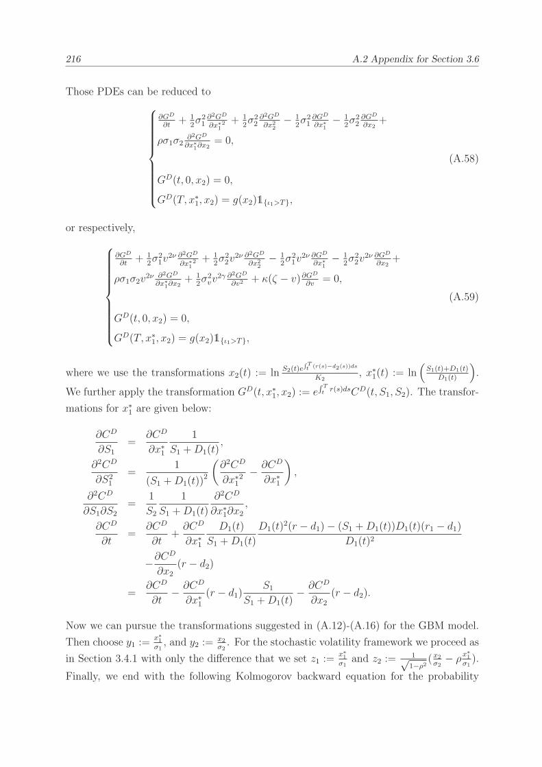
216 A.2 Appendix for Section 3.6
Those PDEs can be reduced to
∂GD
∂t+ 1
2σ21∂2GD
∂x∗12 + 1
2σ22∂2GD
∂x22− 1
2σ21∂GD
∂x∗1− 1
2σ22∂GD
∂x2+
ρσ1σ2∂2GD
∂x∗1∂x2
= 0,
GD(t, 0, x2) = 0,
GD(T, x∗1, x2) = g(x2)1ι1>T,
(A.58)
or respectively,
∂GD
∂t+ 1
2σ21v
2ν ∂2GD
∂x∗12 + 1
2σ22v
2ν ∂2GD
∂x22− 1
2σ21v
2ν ∂GD
∂x∗1− 1
2σ22v
2ν ∂GD
∂x2+
ρσ1σ2v2ν ∂2GD
∂x∗1∂x2
+ 12σ2vv
2γ ∂2GD
∂v2+ κ(ζ − v)∂GD
∂v= 0,
GD(t, 0, x2) = 0,
GD(T, x∗1, x2) = g(x2)1ι1>T,
(A.59)
where we use the transformations x2(t) := ln S2(t)e∫Tt (r(s)−d2(s))ds
K2, x∗1(t) := ln
(S1(t)+D1(t)
D1(t)
)
.
We further apply the transformation GD(t, x∗1, x2) := e∫ Tt
r(s)dsCD(t, S1, S2). The transfor-
mations for x∗1 are given below:
∂CD
∂S1
=∂CD
∂x∗1
1
S1 +D1(t),
∂2CD
∂S21
=1
(S1 +D1(t))2
(∂2CD
∂x∗12 −
∂CD
∂x∗1
)
,
∂2CD
∂S1∂S2
=1
S2
1
S1 +D1(t)
∂2CD
∂x∗1∂x2,
∂CD
∂t=
∂CD
∂t+∂CD
∂x∗1
D1(t)
S1 +D1(t)
D1(t)2(r − d1)− (S1 +D1(t))D1(t)(r1 − d1)
D1(t)2
−∂CD
∂x2(r − d2)
=∂CD
∂t− ∂CD
∂x∗1(r − d1)
S1
S1 +D1(t)− ∂CD
∂x2(r − d2).
Now we can pursue the transformations suggested in (A.12)-(A.16) for the GBM model.
Then choose y1 :=x∗1
σ1, and y2 :=
x2
σ2. For the stochastic volatility framework we proceed as
in Section 3.4.1 with only the difference that we set z1 :=x∗1
σ1and z2 :=
1√1−ρ2
(x2
σ2− ρx∗
1
σ1).
Finally, we end with the following Kolmogorov backward equation for the probability
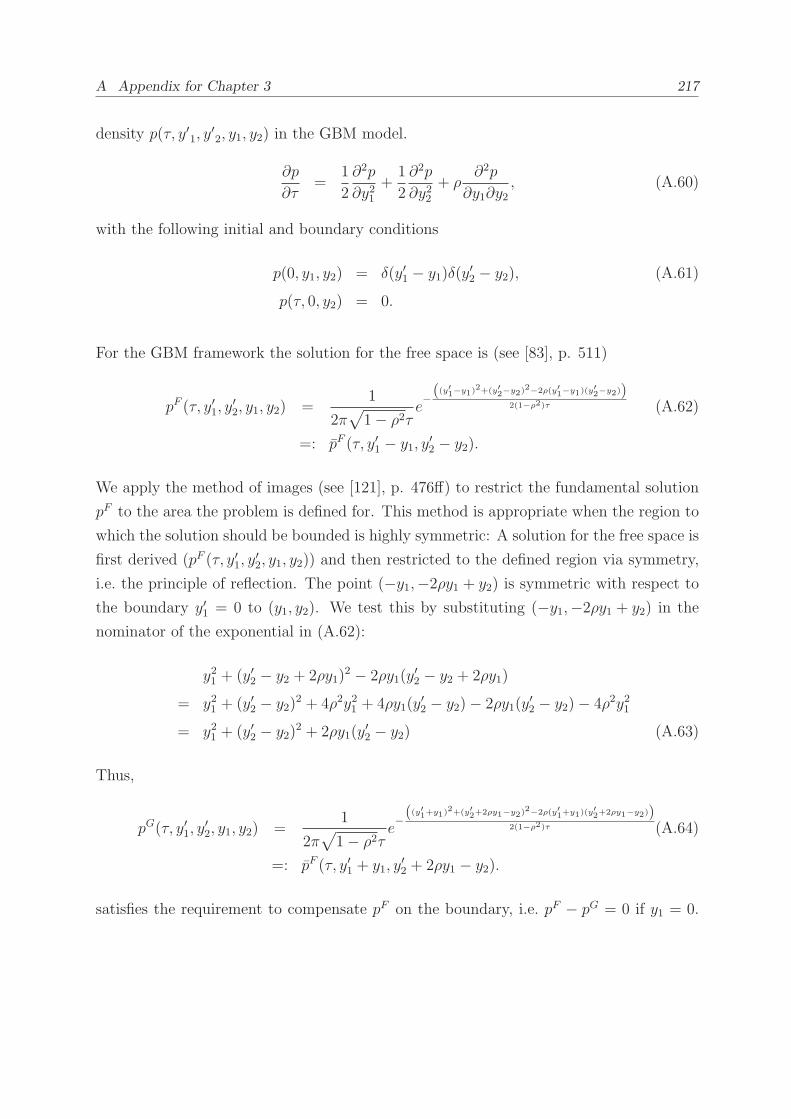
A Appendix for Chapter 3 217
density p(τ, y′1, y′2, y1, y2) in the GBM model.
∂p
∂τ=
1
2
∂2p
∂y21+
1
2
∂2p
∂y22+ ρ
∂2p
∂y1∂y2, (A.60)
with the following initial and boundary conditions
p(0, y1, y2) = δ(y′1 − y1)δ(y′2 − y2), (A.61)
p(τ, 0, y2) = 0.
For the GBM framework the solution for the free space is (see [83], p. 511)
pF (τ, y′1, y′2, y1, y2) =
1
2π√
1− ρ2τe−(
(y′1−y1)2+(y′2−y2)
2−2ρ(y′1−y1)(y′2−y2))
2(1−ρ2)τ (A.62)
=: pF (τ, y′1 − y1, y′2 − y2).
We apply the method of images (see [121], p. 476ff) to restrict the fundamental solution
pF to the area the problem is defined for. This method is appropriate when the region to
which the solution should be bounded is highly symmetric: A solution for the free space is
first derived (pF (τ, y′1, y′2, y1, y2)) and then restricted to the defined region via symmetry,
i.e. the principle of reflection. The point (−y1,−2ρy1 + y2) is symmetric with respect to
the boundary y′1 = 0 to (y1, y2). We test this by substituting (−y1,−2ρy1 + y2) in the
nominator of the exponential in (A.62):
y21 + (y′2 − y2 + 2ρy1)2 − 2ρy1(y
′2 − y2 + 2ρy1)
= y21 + (y′2 − y2)2 + 4ρ2y21 + 4ρy1(y′2 − y2)− 2ρy1(y
′2 − y2)− 4ρ2y21
= y21 + (y′2 − y2)2 + 2ρy1(y′2 − y2) (A.63)
Thus,
pG(τ, y′1, y′2, y1, y2) =
1
2π√
1− ρ2τe−(
(y′1+y1)2+(y′2+2ρy1−y2)
2−2ρ(y′1+y1)(y′2+2ρy1−y2))
2(1−ρ2)τ (A.64)
=: pF (τ, y′1 + y1, y′2 + 2ρy1 − y2).
satisfies the requirement to compensate pF on the boundary, i.e. pF − pG = 0 if y1 = 0.

218 A.2 Appendix for Section 3.6
pG must also satisfy the PDE (A.60):
∂pG
∂τ= −p
G
τ+ pG
((y′1 + y1)2 + (y′2 + 2ρy1 − y2)2 − 2ρ(y′1 + y1)(y
′2 + 2ρy1 − y2))
2(1− ρ2)τ 2 ,
∂pG
∂y1= −pG (y
′1 + y1) + (y′2 − y2 + 2ρy1)2ρ− ρ((y′2 − y2 + 2ρy1) + (y′1 + y1)2ρ)
(1− ρ2)τ
= −pG (y′1 + y1) + ρ(y′2 − y2)− 2ρ2y′1
τ(1− ρ2) ,
∂pG
∂y2= −pG−(y
′2 − y2 + 2ρy1) + ρ(y′1 + y1)
(1− ρ2)τ ,
∂2pG
∂y21= pG
((y′1 + y1) + ρ(y′2 − y2)− 2ρ2y′1)2 − (1− ρ2)τ
(1− ρ2)2τ 2 ,
∂2pG
∂y22= pG
(−(y′2 − y2 + 2ρy1) + ρ(y′1 + y1))2 − (1− ρ2)τ
(1− ρ2)2τ 2 ,
∂2pG
∂y1∂y2= pG
(−(y′2 − y2 + 2ρy1) + ρ(y′1 + y1))((y′1 + y1) + ρ(y′2 − y2)− 2ρ2y′1)
(1− ρ2)2τ 2
+ρ(1− ρ2)τ(1− ρ2)2τ 2p
G.
Thus,
∂pG
∂τ=
1
2
∂2pG
∂y21+
1
2
∂2pG
∂y22+ ρ
∂2pG
∂y1∂y2,
−2τ(1− ρ2) + (y′1 + y1)2 + (y′2 − y2 + 2ρy1)
2 − 2ρ(y′1 + y1)(y′2 − y2 + 2ρy1)
=((y′1 + y1)− 2ρ2(y′1 + y1) + ρ(y′2 − y2 + 2ρy1))
2 − (1− ρ2)τ1− ρ2
+(ρ(y′1 + y1)− (y′2 − y2 + 2ρy1))
2 − (1− ρ2)τ + 2ρ2(1− ρ2)τ1− ρ2
+2ρ (−(y′2 − y2 + 2ρy1) + ρ(y′1 + y1)) ((y
′1 + y1) + ρ(y′2 − y2 + 2ρy1)− 2ρ2(y′1 + y1))
1− ρ2
=−(1− ρ2)2τ(1− ρ2) + (y′2 − y2 + 2ρy1)
2(1 + ρ2 − 2ρ2)
1− ρ2
+(y′1 + y1)
2(ρ2 + 1 + 4ρ4 − 4ρ2 + 2ρ2 − 4ρ4)
1− ρ2
−2ρ(y′1 + y1)(y′2 − y2 + 2ρy1)(1 + (−1 + 2ρ2) + 1− 2ρ2 − ρ2)
1− ρ2= −(1− ρ2)2τ + (y′1 + y1)
2 + (y′2 − y2 + 2ρy1)2 − 2ρ(y′1 + y1)(y
′2 − y2 + 2ρy1).
Hence, with α as in (A.16) and with y1, y2 as defined above the solution for general payoff

A Appendix for Chapter 3 219
functions g(y2) is found by
CD(τ, y1, y2) = ex∗1c1+x2c2−ατ−
∫ Tt
r(s)ds
(∫ ∞
−∞
∫ ∞
−∞pF (τ, y′1 − y1, y′2 − y2)
e−c1x∗1′−c2x
′2g(y′2)dy
′1dy
′2
−∫ ∞
−∞
∫ ∞
0
pF (τ, y1 + y′1, y′2 + 2ρy1 − y2)
e−c1x∗1′−c2x
′2g(y′2)dy
′1dy
′2
)
. (A.65)
For further reference we compute the following double integral
L =1
2π√
1− ρ2τ
∫ ∞
b1
∫ ∞
b2
eγ1y1+γ2y2e− y21+y22−2ρy1y2
2(1−ρ2)τ dy2dy1
=1
2π√
1− ρ2τ
∫ ∞
b1
∫ ∞
b2
eγ1y1+γ2y2e− y21+y22−2ρy1y2
2(1−ρ2)τ
e−−τ2(γ1+ργ2)
2−τ2(γ2+ργ1)2+2y1τ(γ1+ργ2)+2y2τ(γ2+ργ1)
2(1−ρ2)τ
e−−2ρy1τ(γ2+ργ1)−2ρy2τ(γ1+ργ2)+2ρτ2(γ1+ργ2)(γ2+ργ1)
2(1−ρ2)τ dy2dy1
=1
2π√
1− ρ2τ
∫ ∞
b1
∫ ∞
b2
e−−τ(γ21(1+ρ2)+γ22(1+ρ2)+4ργ1γ2)+2γ1y1(1−ρ2)+2γ2y2(1−ρ2)
2(1−ρ2)
e− τ(2ρ2γ21+2ρ2γ22+2ργ1γ2+2ρ3γ1γ2)
2(1−ρ2) e− y21+y22−2ρy1y2
2(1−ρ2)τ eγ1y1+γ2y2dy2dy1
=1
2π√
1− ρ2τ
∫ ∞
b1−τ(γ1+ργ2)
∫ ∞
b2−τ(γ2+ργ1)
eτγ21+γ22+2ργ1γ2
2 e− y21+y22−2ρy1y2
2(1−ρ2)τ dy2dy1
=eτ
γ21+γ22+2ργ1γ22
2π√
1− ρ2∫ ∞
b1√τ−√
τ(γ1+ργ2)
∫ ∞
b2√τ−√
τ(γ2+ργ1)
e− y21+y22−2ρy1y2
2(1−ρ2) dy2dy1
= eτγ21+γ22+2ργ1γ2
2 N2(√τ(γ1 + ργ2)−
b1√τ,√τ(γ2 + ργ1)−
b2√τ; ρ), (A.66)
where y1 = y1 − τ(γ1 + ργ2), y2 = y2 − τ(γ2 + ργ1), and yi =yi√τ.
Furthermore, note that
1
2π√
1− ρ2τe−(
(y′1−y1)2+(y′2−y2)
2−2ρ(y′1−y1)(y′2−y2))
2(1−ρ2)τ
=1
2π√
1− ρ2τe− y′1
2+y′2
2−2ρy′1y
′2+y21+y22−2ρy1y2−2y′1(y1−ρy2)−2y′2(y2−ρy1)
2(1−ρ2)τ (A.67)

220 A.2 Appendix for Section 3.6
and
1
2π√
1− ρ2τe−(
(y′1+y1)2+(y′2−y2+2ρy1)
2−2ρ(y′1+y1)(y′2−y2+2ρy1))
2(1−ρ2)τ
=1
2π√
1− ρ2τe− y′1
2+y′2
2−2ρy′1y
′2+y21+y22−2ρy1y2+2y′1(y1−2ρ2y1+ρy2)−2y′2(y2−ρy1)
2(1−ρ2)τ (A.68)
For the stochastic covariance framework we proceed from (A.59) exactly as in 3.4.1. With
Corollary 5 we can, thus, derive
CD(t, S1, S2, v) =ex
∗1c1+x2c2−
∫ Tt
r(s)ds
4π2σ1σ2√
1− ρ2∫ i2+∞
i2−∞
∫ i1+∞
i1−∞gCD(u1)
(
ϕ(τ,u, z1, z2)− ϕ(τ,u, z1,−z2))
du1du2,
u ∈ SCD = Sϕ ∩ SgCD.
A.2.2 Proof of propositions 4-8
Proof. (Proof of proposition 4)
Thus, with A.65 and g(S2(T )) = S2(T ) = ex′2 in the GBM framework the value of the
index in t is given by
CDS (τ, y1, y2) = ex
∗1c1+x2c2−ατ−
∫ Tt
r(s)ds
(∫ ∞
−∞
∫ ∞
0
pF (τ, y′1 − y1, y′2 − y2)
e−c1x∗1′+(1−c2)x′
2dy′1dy′2
−∫ ∞
−∞
∫ ∞
0
pF (τ, y′1 + y1, y′2 + 2ρy1 − y2)
e−c1x∗1′+(1−c2)x′
2dy′1dy′2
)
,
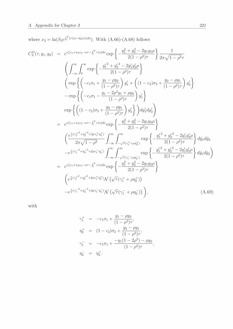
A Appendix for Chapter 3 221
where x2 = ln(S2e∫ Tt(r(s)−d2(s))ds). With (A.66)-(A.68) follows
CDS (τ, y1, y2) = ex
∗1c1+x2c2−ατ−
∫ Tt
r(s)ds exp
−y21 + y22 − 2y1y2ρ
2(1− ρ2)τ
1
2π√
1− ρ2τ(∫ ∞
−∞
∫ ∞
0
exp
−y′12 + y′2
2 − 2y′1y′2ρ
2(1− ρ2)τ
(
exp
(
−c1σ1 +y1 − ρy2(1− ρ2)τ
)
y′1 +
(
(1− c2)σ2 +y2 − ρy1(1− ρ2)τ
)
y′2
− exp
(
−c1σ1 −y1 − 2ρ2y1 + ρy2
(1− ρ2)τ
)
y′1
exp
(
(1− c2)σ2 +y2 − ρy1(1− ρ2)τ
)
y′2
)
dy′1dy′2
)
= ex∗1c1+x2c2−ατ−
∫ Tt
r(s)ds exp
−y21 + y22 − 2y1y2ρ
2(1− ρ2)τ
(e
τ2(γ+
12+η+2
2+2ργ+
1 η+2 )
2π√
1− ρ2∫ ∞
−∞
∫ ∞
−√τ(γ+
1 +ρη+2 )
exp
−y′12 + y′2
2 − 2y′1y′2ρ
2(1− ρ2)τ
dy1dy2
−e τ2(γ−
12+η−2
2+2ργ−
1 η−2 )
∫ ∞
−∞
∫ ∞
−√τ(γ−
1 +ρη−2 )
exp
−y′12 + y′2
2 − 2y′1y′2ρ
2(1− ρ2)τ
dy1dy2
)
= ex∗1c1+x2c2−ατ−
∫ Tt
r(s)ds exp
−y21 + y22 − 2y1y2ρ
2(1− ρ2)τ
(
eτ2(γ+
1
2+η+2
2+2ργ+
1 η+2 )N(√
τ(γ+1 + ρη+2 ))
−e τ2(γ−
12+η−2
2+2ργ−
1 η−2 )N(√
τ(γ−1 + ρη−2 )))
, (A.69)
with
γ+1 = −c1σ1 +y1 − ρy2(1− ρ2)τ ,
η+2 = (1− c2)σ2 +y2 − ρy1(1− ρ2)τ ,
γ−1 = −c1σ1 +−y1(1− 2ρ2)− ρy2
(1− ρ2)τ ,
η−2 = η+2 .

222 A.2 Appendix for Section 3.6
To simplify we calculate
d1 :=√τ(γ+1 + ρη+2 ) =
√τ
(
−c1σ1 + ρ(1− c2)σ2 +x∗1σ1τ
)
=√τ
(
− σ1 − ρσ22(1− ρ2) + ρ
σ2(1− 2ρ2) + ρσ12(1− ρ2) +
x∗1σ1τ
)
=x∗1
σ1√τ− σ1
√τ
2+ ρσ2
√τ ,
d1 :=√τ(γ−1 + ρη−2 ) =
√τ
(
− σ1 − ρσ22(1− ρ2) + ρ
σ2(1− 2ρ2) + ρσ12(1− ρ2) − x∗1
σ1τ
)
= − x∗1σ1√τ− σ1
√τ
2+ ρσ2
√τ ,
τ
2(γ+1
2+ η+2
2+ 2ργ+1 η
+2 ) =
τ
2
(
c21σ21 + (1− c2)2σ2
2 − 2ρσ1σ2c1(1− c2)
+
(y1 − ρy2(1− ρ2)τ
)2
− 2c1σ1y1 − ρy2(1− ρ2)τ +
(y2 − ρy1(1− ρ2)τ
)2
+2(1− c2)σ2y2 − ρy1(1− ρ2)τ + 2ρ(1− c2)σ2
y1 − ρy2(1− ρ2)τ
−2ρc1σ1y2 − ρy1(1− ρ2)τ + 2ρ
(y2 − ρy1)(y1 − ρy2)(1− ρ2)2τ 2
)
=τ
2
(
σ21
(σ1 − ρσ2σ1(1− ρ2)2
)2
+
(σ2 − ρσ1σ2(1− ρ2)2
)2
σ22
+2ρσ1σ2σ1 − ρσ2σ1(1− ρ2)2
σ2 − ρσ1σ2(1− ρ2)2
+ σ22 − 2c2σ
22 − 2ρc1σ1σ2
−2c1σ1y1τ
+ 2(1− c2)σ2y2τ
+y21(1 + ρ2 − 2ρ2) + y22(ρ
2 + 1− 2ρ2)− 2ρy1y2(1− ρ2)(1− ρ2)2τ 2
)
=τ
2
(σ21(1− ρ2) + σ2
2(1− ρ2)− 2ρσ1σ2(1− ρ2)4(1− ρ2)2
+σ22 − σ2
σ2 − ρσ11− ρ2 − σ2
ρσ1 − ρ2σ21− ρ2
)
+
(
−c1x∗1 + (1− c2)x2 +y21 + y22 − 2ρy1y2
2(1− ρ2)τ
)
= ατ − c1x∗1 + (1− c2)x2 +y21 + y22 − 2ρy1y2
2(1− ρ2)τ , (A.70)
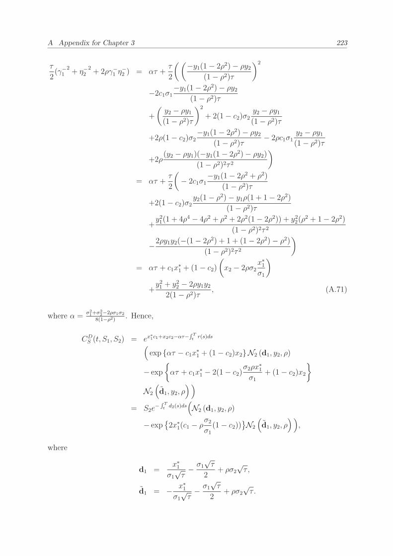
A Appendix for Chapter 3 223
τ
2(γ−1
2+ η−2
2+ 2ργ−1 η
−2 ) = ατ +
τ
2
((−y1(1− 2ρ2)− ρy2(1− ρ2)τ
)2
−2c1σ1−y1(1− 2ρ2)− ρy2
(1− ρ2)τ
+
(y2 − ρy1(1− ρ2)τ
)2
+ 2(1− c2)σ2y2 − ρy1(1− ρ2)τ
+2ρ(1− c2)σ2−y1(1− 2ρ2)− ρy2
(1− ρ2)τ − 2ρc1σ1y2 − ρy1(1− ρ2)τ
+2ρ(y2 − ρy1)(−y1(1− 2ρ2)− ρy2)
(1− ρ2)2τ 2)
= ατ +τ
2
(
− 2c1σ1−y1(1− 2ρ2 + ρ2)
(1− ρ2)τ
+2(1− c2)σ2y2(1− ρ2)− y1ρ(1 + 1− 2ρ2)
(1− ρ2)τ
+y21(1 + 4ρ4 − 4ρ2 + ρ2 + 2ρ2(1− 2ρ2)) + y22(ρ
2 + 1− 2ρ2)
(1− ρ2)2τ 2
−2ρy1y2(−(1− 2ρ2) + 1 + (1− 2ρ2)− ρ2)(1− ρ2)2τ 2
)
= ατ + c1x∗1 + (1− c2)
(
x2 − 2ρσ2x∗1σ1
)
+y21 + y22 − 2ρy1y2
2(1− ρ2)τ , (A.71)
where α =σ21+σ2
2−2ρσ1σ2
8(1−ρ2). Hence,
CDS (t, S1, S2) = ex
∗1c1+x2c2−ατ−
∫ Tt
r(s)ds
(
exp ατ − c1x∗1 + (1− c2)x2N2 (d1, y2, ρ)
− exp
ατ + c1x∗1 − 2(1− c2)
σ2ρx∗1
σ1+ (1− c2)x2
N2
(
d1, y2, ρ))
= S2e−∫ Tt
d2(s)ds(
N2 (d1, y2, ρ)
− exp2x∗1(c1 − ρ
σ2σ1
(1− c2))N2
(
d1, y2, ρ))
,
where
d1 =x∗1
σ1√τ− σ1
√τ
2+ ρσ2
√τ ,
d1 = − x∗1σ1√τ− σ1
√τ
2+ ρσ2
√τ .

224 A.2 Appendix for Section 3.6
For the stochastic covariance framework we have to derive hDS (u1, u2) using the transfor-
mations in Section A.2.1 analogue to (3.43).
hDS (u1, u2) =
∫ ∞
0
∫ ∞
−∞e−c1x
∗1′+(1−c2)x′
2eiu1z′1+iu2z
′2dx′2dx
∗1′
=
∫ ∞
0
∫ ∞
−∞e−c1x
∗1′+(1−c2)x′
2e
(
x∗1′
σ1
(
− ρ√1−ρ2
iu2+iu1
)
+iu2x′2
σ2
√1−ρ2
)
dx′2dx∗1′
=
∫ ∞
0
∫ ∞
0
e−c1x∗1′e(1−c2)x′
2e
(
x∗1′
σ1
(
− ρ√1−ρ2
iu2+iu1
)
+iu2x′2
σ2
√1−ρ2
)
dx′2dx∗1′
+
∫ ∞
0
∫ 0
−∞e−c1x
∗1′e(1−c2)x′
2e
(
x∗1′
σ1
(
− ρ√1−ρ2
iu2+iu1
)
+iu2x′2
σ2
√1−ρ2
)
dx′2dx∗1′
=
∫ ∞
0
e−c1x∗1′e
x∗1′
σ1
(
− ρ√1−ρ2
iu2+iu1
)(
− 1iu2
σ2
√1−ρ2
+ 1− c2
2>(1−c2)σ2
√1−ρ2
+
1
iu2
σ2
√1−ρ2
+ 1− c2
2<(1−c2)σ2
√1−ρ2
)
dx∗1′.
Note that we can set ℑ(u2) = 2 = 0 for the second (first) fraction if c2 < 1 (c2 > 1).
Then we can move the path of integration of the first (second) bracket to the real axis
with Corollary 3. We compute with (2.56) the residue of the integrand f of hDS at u2 =
i(1− c2)σ2√
1− ρ2.
Resu2f = limu2→u1
(
u2 − iσ2√
1− ρ2(1− c2))
− σ2√
1− ρ2
i(
u2 − iσ2√
1− ρ2(1− c2))
= iσ2√
1− ρ2 (A.72)
When we set now the path with Corollary 3 to 2 = 0 the fractions cancel and we are
left with a Dirac delta function. Thus,
hDS (u1, u2) =
∫ ∞
0
e−c1x∗1′e
x∗1′
σ1
(
− ρ√1−ρ2
iu2+iu1
)
(
− 2πiσ2√
1− ρ2iδ(u2 − iσ2√
1− ρ2(1− c2)))
dx∗1′
=
− σ2√
1− ρ22πiu1
σ1− ρiu2√
1−ρ2σ1
− c1
1>(−σ1c1+(1−c2)σ2ρ),2=0
δ(u2 − iσ2√
1− ρ2(1− c2)).
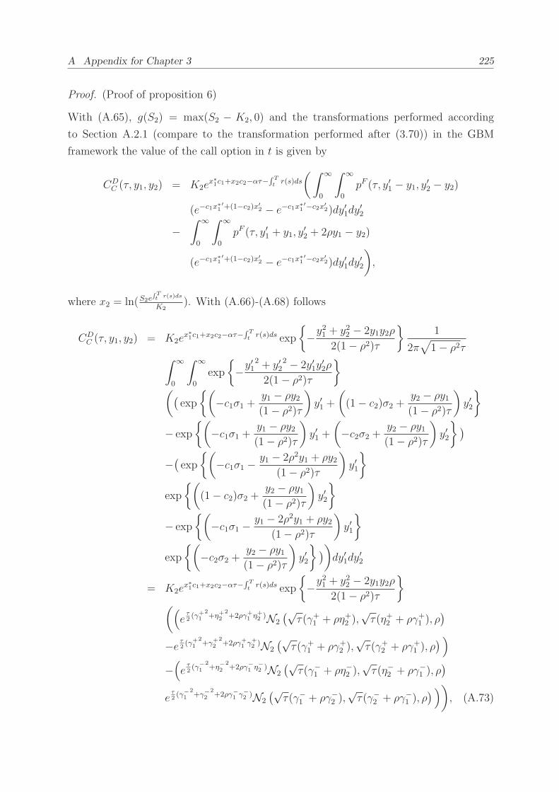
A Appendix for Chapter 3 225
Proof. (Proof of proposition 6)
With (A.65), g(S2) = max(S2 − K2, 0) and the transformations performed according
to Section A.2.1 (compare to the transformation performed after (3.70)) in the GBM
framework the value of the call option in t is given by
CDC (τ, y1, y2) = K2e
x∗1c1+x2c2−ατ−
∫ Tt
r(s)ds
(∫ ∞
0
∫ ∞
0
pF (τ, y′1 − y1, y′2 − y2)
(e−c1x∗1′+(1−c2)x′
2 − e−c1x∗1′−c2x
′2)dy′1dy
′2
−∫ ∞
0
∫ ∞
0
pF (τ, y′1 + y1, y′2 + 2ρy1 − y2)
(e−c1x∗1′+(1−c2)x′
2 − e−c1x∗1′−c2x
′2)dy′1dy
′2
)
,
where x2 = ln(S2e∫Tt r(s)ds
K2). With (A.66)-(A.68) follows
CDC (τ, y1, y2) = K2e
x∗1c1+x2c2−ατ−
∫ Tt
r(s)ds exp
−y21 + y22 − 2y1y2ρ
2(1− ρ2)τ
1
2π√
1− ρ2τ∫ ∞
0
∫ ∞
0
exp
−y′12 + y′2
2 − 2y′1y′2ρ
2(1− ρ2)τ
((exp
(
−c1σ1 +y1 − ρy2(1− ρ2)τ
)
y′1 +
(
(1− c2)σ2 +y2 − ρy1(1− ρ2)τ
)
y′2
− exp
(
−c1σ1 +y1 − ρy2(1− ρ2)τ
)
y′1 +
(
−c2σ2 +y2 − ρy1(1− ρ2)τ
)
y′2
)
−(exp
(
−c1σ1 −y1 − 2ρ2y1 + ρy2
(1− ρ2)τ
)
y′1
exp
(
(1− c2)σ2 +y2 − ρy1(1− ρ2)τ
)
y′2
− exp
(
−c1σ1 −y1 − 2ρ2y1 + ρy2
(1− ρ2)τ
)
y′1
exp
(
−c2σ2 +y2 − ρy1(1− ρ2)τ
)
y′2
))
dy′1dy′2
= K2ex∗1c1+x2c2−ατ−
∫ Tt
r(s)ds exp
−y21 + y22 − 2y1y2ρ
2(1− ρ2)τ
((
eτ2(γ+
12+η+2
2+2ργ+
1 η+2 )N2
(√τ(γ+1 + ρη+2 ),
√τ(η+2 + ργ+1 ), ρ
)
−e τ2(γ+
12+γ+
22+2ργ+
1 γ+2 )N2
(√τ(γ+1 + ργ+2 ),
√τ(γ+2 + ργ+1 ), ρ
) )
−(
eτ2(γ−
12+η−2
2+2ργ−
1 η−2 )N2
(√τ(γ−1 + ρη−2 ),
√τ(η−2 + ργ−1 ), ρ
)
eτ2(γ−
1
2+γ−
2
2+2ργ−
1 γ−2 )N2
(√τ(γ−1 + ργ−2 ),
√τ(γ−2 + ργ−1 ), ρ
) ))
, (A.73)

226 A.2 Appendix for Section 3.6
with
γ+1 = −c1σ1 +y1 − ρy2(1− ρ2)τ ,
η+2 = (1− c2)σ2 +y2 − ρy1(1− ρ2)τ ,
γ+2 = −c2σ2 +y2 − ρy1(1− ρ2)τ ,
γ−1 = −c1σ1 +−y1(1− 2ρ2)− ρy2
(1− ρ2)τ ,
η−2 = η+2 ,
γ−2 = γ+2 .
To simplify we calculate
d∗1 :=√τ(γ+1 + ργ+2 ) =
√τ
(
−c1σ1 − ρc2σ2 +x∗1σ1τ
)
=√τ
(
− σ1 − ρσ22(1− ρ2) − ρ
σ2 − ρσ12(1− ρ2) +
x∗1σ1τ
)
=x∗1
σ1√τ− σ1
√τ
2,
d∗1 :=√τ(γ−1 + ργ−2 ) =
√τ
(
− σ1 − ρσ22(1− ρ2) − ρ
σ2 − ρσ12(1− ρ2) −
x∗1σ1τ
)
= − x∗1σ1√τ− σ1
√τ
2,
d2 :=√τ(η+2 + ργ+1 ) =
√τ
(
(1− c2)σ2 − ρc1σ1 +x2σ2τ
)
=x2
σ2√τ+√τ
(σ2(1− 2ρ2) + ρσ1
2(1− ρ2) − ρ σ1 − ρσ22(1− ρ2)
)
=x2
σ2√τ+
1
2
√τσ2,
d∗2 :=√τ(γ+2 + ργ+1 ) =
√τ
(
−c2σ2 − ρc1σ1 +x2σ2τ
)
=x2
σ2√τ+√τ
(
− σ2 − ρσ12(1− ρ2) − ρ
σ1 − ρσ22(1− ρ2)
)
=x2
σ2√τ− 1
2
√τσ2,
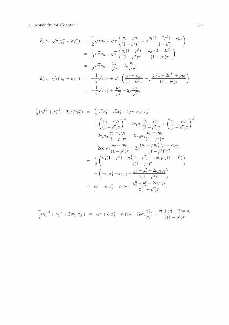
A Appendix for Chapter 3 227
d2 :=√τ(η−2 + ργ−1 ) =
1
2
√τσ2 +
√τ
(y2 − ρy1(1− ρ2)τ − ρ
y1(1− 2ρ2) + ρy1(1− ρ2)τ
)
=1
2
√τσ2 +
√τ
(y2(1− ρ2)(1− ρ2)τ −
ρy1(2− 2ρ2)
(1− ρ2)τ
)
=1
2
√τσ2 +
y2√τ− 2ρ
y1√τ,
d∗2 :=√τ(γ−2 + ργ−1 ) = −1
2
√τσ2 +
√τ
(y2 − ρy1(1− ρ2)τ − ρ
y1(1− 2ρ2) + ρy1(1− ρ2)τ
)
= −1
2
√τσ2 +
y2√τ− 2ρ
y1√τ,
τ
2(γ+1
2+ γ+2
2+ 2ργ+1 γ
+2 ) =
τ
2(c21σ
21 − c22σ2
2 + 2ρσ1σ2c1c2)
+
(y1 − ρy2(1− ρ2)τ
)2
− 2c1σ1y1 − ρy2(1− ρ2)τ +
(y2 − ρy1(1− ρ2)τ
)2
−2c2σ2y2 − ρy1(1− ρ2)τ − 2ρc2σ2
y1 − ρy2(1− ρ2)τ
−2ρc1σ1y2 − ρy1(1− ρ2)τ + 2ρ
(y2 − ρy1)(y1 − ρy2)(1− ρ2)2τ 2
=τ
2
(σ21(1− ρ2) + σ2
2(1− ρ2)− 2ρσ1σ2(1− ρ2)4(1− ρ2)2
)
+
(
−c1x∗1 − c2x2 +y21 + y22 − 2ρy1y2
2(1− ρ2)τ
)
= ατ − c1x∗1 − c2x2 +y21 + y22 − 2ρy1y2
2(1− ρ2)τ ,
τ
2(γ−1
2+ γ−2
2+ 2ργ−1 γ
−2 ) = ατ + c1x
∗1 − c2(x2 − 2ρσ2
x∗1σ1
) +y21 + y22 − 2ρy1y2
2(1− ρ2)τ ,

228 A.2 Appendix for Section 3.6
CDC (t, S1, S2, K2) = K2e
x∗1c1+x2c2−ατ−
∫ Tt
r(s)ds
((
exp −c1x∗1 + (1− c2)x2 + ατN2 (d1,d2, ρ)
− exp −c1x∗1 − c2x2 + ατN2 (d∗1,d
∗2, ρ)
)
−(
exp
ατ + c1x∗1 − 2(1− c2)
σ2ρx∗1
σ1+ (1− c2)x2
N2
(
d1, d2, ρ)
− exp
ατ + c1x∗1 + 2c2
σ2ρx∗1
σ1− c2x2
N2
(
d∗1, d
∗2, ρ)))
=
((
S2e−∫ Tt
d2(s)dsN2 (d1,d2, ρ)−K2e−∫ Tt
r(s)dsN2 (d∗1,d
∗2, ρ)
)
−(
S2e−∫ Tt
d2(s)ds exp
2x∗1(c1 − (1− c2)σ2ρ
σ1)
N2
(
d1, d2, ρ)
−K2e−∫ Tt
r(s)ds exp
2x∗1(c1 + c2σ2ρ
σ1)
N2
(
d∗1, d
∗2, ρ)))
,
where
d1 =x∗1
σ1√τ− 1
2σ1√τ + ρσ2
√τ , d2 =
x2σ2√τ+
1
2σ2√τ ,
d1 = − x∗1
σ1√τ− 1
2σ1√τ + ρσ2
√τ , d2 =
x2σ2√τ− 2ρ
x∗1σ1√τ+
1
2σ2√τ ,
d∗1 = d1 − ρσ2
√τ , d∗
2 = d2 − σ2√τ ,
d∗1 = d1 − ρσ2
√τ , d∗
2 = d2 − σ2√τ .
For the stochastic covariance framework we derive hDC :
hDC (u1, u2) = K2
∫ ∞
0
∫ ∞
0
e−c1x∗1′(
ex′2(1−c2) − e−x′
2c2
)
e
(
x∗1′
σ1
(
− ρ√1−ρ2
iu2+iu1
)
+iu2x′2
σ2
√1−ρ2
)
dx′2dx∗1′
= K21
i
(
u1
σ1− u2ρ
σ1
√1−ρ2
)
− c1
1(
i u2
σ2
√1−ρ2
+ 1− c2)(
i u2
σ2
√1−ρ2− c2
) .
Note that we have to set ℑ(u2) > σ2√
1− ρ2(1− c2) and ℑ(u1) > ρ√1−ρ2ℑ(u2)− σ1c1, i.e
SgDC=
u = w + i : 2 > σ2√
1− ρ2(1− c2) ∧1 >ρ√1−ρ2
2 − σ1c1
.

A Appendix for Chapter 3 229
Proof. (Proof of proposition 7)
Analogue to the proof above for the call option the value of the digital call option in t in
the GBM framework with payoff g(S2) = 1S2(T )>K (for the transformation compare with
the explanations after (3.66)) follows
CDD (t, S1, S2, K2) = e−
∫ Tt
r(s)ds
(
N2 (d∗1,d
∗2, ρ)− exp
2x∗1(c1 + c2σ2ρ
σ1)
N2
(
d∗1, d
∗2, ρ))
,
and,
d∗2 =
x2σ2√τ− 1
2σ2√τ , d∗
2 =x2
σ2√τ− 2ρ
x∗1σ1√τ− 1
2σ2√τ .
The result for the stochastic covariance framework follows with Corollary 5 with b2 = 0
.
Proof. (Proof of proposition 8)
(A.60) with additional boundary condition p(τ, y1, b2) = 0 can be solved by applying
Theorem 36 in connection with Remark 14.
(A.59) with the additional boundary condition is solved by the application of Theorem
36. The results follow.

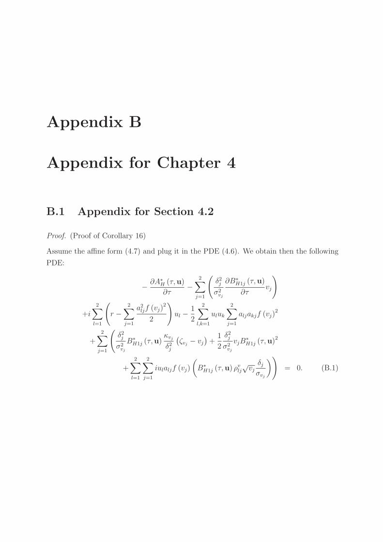
Appendix B
Appendix for Chapter 4
B.1 Appendix for Section 4.2
Proof. (Proof of Corollary 16)
Assume the affine form (4.7) and plug it in the PDE (4.6). We obtain then the following
PDE:
− ∂A∗H (τ,u)
∂τ−
2∑
j=1
(
δ2jσ2vj
∂B∗H1j (τ,u)
∂τvj
)
+i2∑
l=1
(
r −2∑
j=1
a2ljf (vj)2
2
)
ul −1
2
2∑
l,k=1
uluk
2∑
j=1
aljakjf (vj)2
+2∑
j=1
(
δ2jσ2vj
B∗H1j (τ,u)
κvjδ2j
(ζvj − vj
)+
1
2
δ2jσ2vj
vjB∗H1j (τ,u)
2
+2∑
l=1
2∑
j=1
iulaljf (vj)
(
B∗H1j (τ,u) ρ
vlj
√vjδjσvj
))
= 0. (B.1)
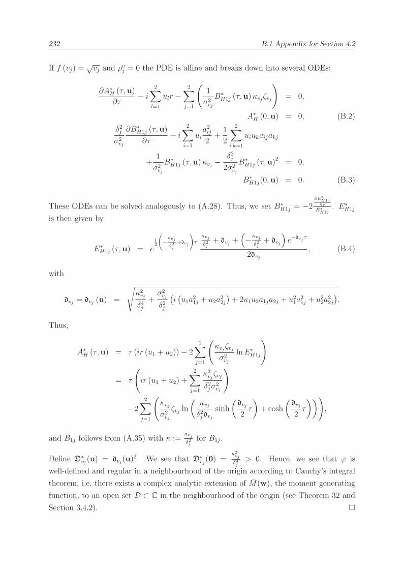
232 B.1 Appendix for Section 4.2
If f (vj) =√vj and ρ
vj = 0 the PDE is affine and breaks down into several ODEs:
∂A∗H (τ,u)
∂τ− i
2∑
l=1
ulr −2∑
j=1
(
1
σ2vj
B∗H1j (τ,u)κvjζvj
)
= 0,
A∗H (0,u) = 0, (B.2)
δ2jσ2vj
∂B∗H1j (τ,u)
∂τ+ i
2∑
i=1
uia2ij2
+1
2
2∑
i,k=1
uiukaijakj
+1
σ2vj
B∗H1j (τ,u)κvj −
δ2j2σ2
vj
B∗H1j (τ,u)
2 = 0,
B∗H1j(0,u) = 0. (B.3)
These ODEs can be solved analogously to (A.28). Thus, we set B∗H1j = −2
∂E∗H1j∂τ
E∗H1j
. E∗H1j
is then given by
E∗H1j (τ,u) = e
12
(
−κvj
δ2j
+dvj
)
τ
κvj
δ2j+ dvj +
(
−κvj
δ2j+ dvj
)
e−dvj τ
2dvj, (B.4)
with
dvj = dvj (u) =
√
κ2vjδ4j
+σ2vj
δ2j
(i(u1a21j + u2a22j
)+ 2u1u2a1ja2j + u21a
21j + u22a
22j
).
Thus,
A∗H (τ,u) = τ (ir (u1 + u2))− 2
2∑
j=1
(
κvjζvjσ2vj
lnE∗H1j
)
= τ
(
ir (u1 + u2) +2∑
j=1
κ2vjζvj
δ2jσ2vj
)
−22∑
j=1
(
κvjσ2vj
ζvj ln
(κvjδ2jdvj
sinh
(dvj
2τ
)
+ cosh
(dvj
2τ
)))
,
and B1j follows from (A.35) with κ :=κvj
δ2jfor B1j.
Define D∗vj(u) = dvj(u)
2. We see that D∗vj(0) =
κ2vj
δ4j> 0. Hence, we see that ϕ is
well-defined and regular in a neighbourhood of the origin according to Cauchy’s integral
theorem, i.e. there exists a complex analytic extension of M(w), the moment generating
function, to an open set D ⊂ C in the neighbourhood of the origin (see Theorem 32 and
Section 3.4.2).
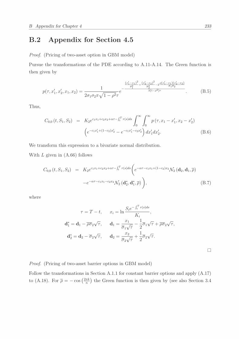
B Appendix for Chapter 4 233
B.2 Appendix for Section 4.5
Proof. (Pricing of two-asset option in GBM model)
Pursue the transformations of the PDE according to A.11-A.14. The Green function is
then given by
p(τ, x′1, x′2, x1, x2) =
1
2σ1σ2π√
1− ρ2τe−
(x′1−x1)2
σ21
+(x′2−x2)
2
σ22
−2ρ(x′1−x1)(x
′2−x2)
σ1σ2
2(1−ρ2)τ . (B.5)
Thus,
C0,0 (t, S1, S2) = K2ec1x1+c2x2+ατ−
∫ Tt
r(s)ds
∫ ∞
0
∫ ∞
0
p (τ, x1 − x′1, x2 − x′2)(
e−c1x′1+(1−c2)x′
2 − e−c1x′1−c2x
′2
)
dx′1dx′2. (B.6)
We transform this expression to a bivariate normal distribution.
With L given in (A.66) follows
C0,0 (t, S1, S2) = K2ec1x1+c2x2+ατ−
∫ Tt
r(s)ds
(
e−ατ−c1x1+(1−c2)x2N2 (d2,d1, ρ)
−e−ατ−c1x1−c2x2N2 (d∗2,d
∗1, ρ)
)
, (B.7)
where
τ = T − t, xi = lnSie
−∫ Tt
r(s)ds
Ki
,
d∗1 = d1 − ρσ2
√τ , d1 =
x1σ1
√τ− 1
2σ1
√τ + ρσ2
√τ ,
d∗2 = d2 − σ2
√τ , d2 =
x2σ2
√τ+
1
2σ2
√τ .
Proof. (Pricing of two-asset barrier options in GBM model)
Follow the transformations in Section A.1.1 for constant barrier options and apply (A.17)
to (A.18). For ρ = − cos(2πkn
)the Green function is then given by (see also Section 3.4
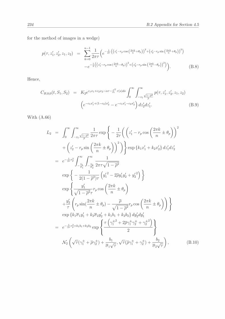
234 B.2 Appendix for Section 4.5
for the method of images in a wedge)
p(τ, z′1, z′2, z1, z2) =
n−1∑
k=0
1
2πτ
(
e− 1
2τ
(
(z′1−rp cos ( 2πkn
+θp))2+(z′2−rp sin ( 2πk
n+θp))
2)
−e−12
(
(z′1−rp cos ( 2πkn
−θp))2+(z′2−rp sin ( 2πk
n−θp))
2))
. (B.8)
Hence,
CB,0,0(t, S1, S2) = K2ec1x1+c2x2−ατ−
∫ Tt
r(s)ds
∫ ∞
0
∫ ∞
−z1
√1−ρ2
ρ
p(τ, z′1, z′2, z1, z2)
(
e−c1x′1+(1−c2)x′
2 − e−c1x′1−c2x
′2
)
dz′2dz′1. (B.9)
With (A.66)
L2 =
∫ ∞
0
∫ ∞
−z1
√1−ρ2
ρ
1
2πτexp
− 1
2τ
((
z′1 − rp cos(2πk
n± θp
))2
+
(
z′2 − rp sin(2πk
n± θp
))2)
exp k1x′1 + k2x′2 dz′1dz′2
= e−12τ
r2p
∫ ∞
− b1σ1
∫ ∞
− b2σ2
1
2πτ√
1− ρ2
exp
− 1
2(1− ρ2)τ(
y′12 − 2ρy′1y
′2 + y′2
2)
exp
y′1√
1− ρ2τrp cos
(2πk
n± θp
)
+y′2τ
(
rp sin(2πk
n± θp)−
ρ√
1− ρ2rp cos
(2πk
n± θp
))
exp k1σ1y′1 + k2σ2y
′2 + k1b1 + k2b2 dy′2dy′1
= e−12τ
r2p+k1b1+k2b2 exp
τ(
γ±12+ 2ργ±1 γ
±2 + γ±2
2)
2
N2
(√τ(γ±1 + ργ±2 ) +
b1σ1
√τ,√τ(ργ±1 + γ±2 ) +
b2σ2
√τ
)
, (B.10)
B Appendix for Chapter 4 235
where yi =xi−biσi
, z21 := 1(1−ρ2)
(y1 − ρy2)2 = 1(1−ρ2)
(y21 + y22ρ2 − 2y1y2ρ), and z
22 := y22,
γ±1 =1
τ√
1− ρ2rp cos
(2πk
n
+− θp
)
+ k1σ1
=1
τ√
1− ρ2(
rp cos(2πk
n) cos(θp)
−+ rp sin(
2πk
n) sin(θp)
)
+ k1σ1
=1
τ√
1− ρ2(
z1 cos(2πk
n)
−+ z2 sin(
2πk
n)
)
+ k1σ1
=1
τ√
1− ρ2
(
1√
1− ρ2(y1 − ρy2) cos(
2πk
n)
−+ y2 sin(
2πk
n)
)
+ k1σ1
= k1σ1 + y11
τ(1− ρ2) cos(2πk
n
)
+y2
(
−+
1
τ√
1− ρ2sin
(2πk
n
)
− ρ
τ (1− ρ2) cos(2πk
n
))
, (B.11)
γ±2 =1
τ√
1− ρ2(√
1− ρ2rp sin(2πk
n
+− θp
)
− ρrp cos(2πk
n
+− θp
))
+ k2σ2
=1
τ√
1− ρ2
(√
1− ρ2(
+− rp sin(θp) cos(
2πk
n) + rp cos(θp) sin(
2πk
n)
)
−ρ(
rp cos(2πk
n) cos(θp)
−+ rp sin(
2πk
n) sin(θp)
))
+ k2σ2
=1
τ√
1− ρ2
(√
1− ρ2(
+− z2 cos(
2πk
n) + z1 sin(
2πk
n)
)
−ρ(
z1 cos(2πk
n)
−+ z2 sin(
2πk
n)
))
+ k2σ2
=1
τ√
1− ρ2
(√
1− ρ2(
+− y2 cos(
2πk
n) +
1√
1− ρ2(y1 − ρy2) sin(
2πk
n)
)
−ρ(
1√
1− ρ2(y1 − ρy2) cos(
2πk
n)
−+ y2 sin(
2πk
n)
))
+ k2σ2

236 B.2 Appendix for Section 4.5
= 1
τ√
1−ρ2
(
y2
(√
1− ρ2 cos(2πkn
)+ ρ2√
1−ρ2cos(2πkn
))
+y1
(
sin(2πkn
)− ρ√
1−ρ2cos(2πkn
)))
+ k2σ2 for γ+2
= 1
τ√
1−ρ2
(
y2
(
−√
1− ρ2 cos(2πkn
)+ ρ2√
1−ρ2cos(2πkn
)− 2ρ sin(2πk
n)
)
+y1
(
sin(2πkn
)− ρ√
1−ρ2cos(2πkn
)))
+ k2σ2 for γ−2
= 1
τ√
1−ρ2
(
y21√1−ρ2
cos(2πkn
)
+y1
(
sin(2πkn
)− ρ√
1−ρ2cos(2πkn
)))
+ k2σ2 for γ+2
= 1
τ√
1−ρ2
(
y2
(
− 1−2ρ2√1−ρ2
cos(2πkn
)− 2ρ sin(2πk
n)
)
+y1
(
sin(2πkn
)− ρ√
1−ρ2cos(2πkn
)))
+ k2σ2 for γ−2
(B.12)
B Appendix for Chapter 4 237
Hence, CB,0,0 is given by
CB,0,0(t, S1, S2) =n−1∑
k=0
ec1x1+c2x2−ατe−12τ
r2p−c1b1−c2b2 (B.13)
(
B2
(
exp
τ(
γ+12+ 2ργ+1 η
+2 + η+2
2)
2
N2
(√τ(γ+1 + ρη+2 ) +
b1σ1
√τ,√τ(ργ+1 + η+2 ) +
b2σ2
√τ
)
− exp
τ(
γ−12+ 2ργ−1 η
−2 + η−2
2)
2
N2
(√τ(γ−1 + ρη−2 ) +
b1σ1
√τ,√τ(ργ−1 + η−2 ) +
b2σ2
√τ
))
−K2e−∫ Tt
r(s)ds
(
exp
τ(
γ+12+ 2ργ+1 γ
+2 + γ+2
2)
2
N2
(√τ(γ+1 + ργ+2 ) +
b1σ1
√τ,√τ(ργ+1 + γ+2 ) +
b2σ2
√τ
)
− exp
τ(
γ−12+ 2ργ−1 γ
−2 + γ−2
2)
2
N2
(√τ(γ−1 + ργ−2 ) +
b1σ1
√τ,√τ(ργ−1 + γ−2 ) +
b2σ2
√τ
)))
,
where γ±1 , γ±2 are as indicated in (B.11)-(B.12) with k1 = −c1 and k2 = −c2, η±2 follows
γ±2 with k2 = (1− c2).
Now, we simplify the singular multiplying factors of the normal distributions
by inserting (B.11)-(B.12) and we use our calculations in (A.70) for ατ , i.e.τ2(c21σ
21 + (1− c2)2σ2
2 − 2ρσ1σ2c1(1− c2)) = τ2(c21σ
21 + c22σ
22 + 2ρσ1σ2c1c2) = ατ .

238 B.2 Appendix for Section 4.5
τ
2(γ±1
2+ 2ργ±1 η
±2 + η±2
2)
=τ
2
(c21σ
21 + (1− c2)2σ2
2 − 2ρc1(1− c2)σ1σ2
)
+τ
2
(
1
τ 2(1− ρ2)r2p cos
(2πk
n± θp
)
+1
τ 2(1− ρ2)(
(1− ρ2)r2p sin2
(2πk
n± θp
)
+ ρ2r2p cos2
(2πk
n± θp
))
−2ρ√
1− ρ2r2p cos(2πk
n± θp
)
sin
(2πk
n± θp
)
+2ρ
τ 2(1− ρ2)
(√
1− ρ2r2p sin(2πk
n± θp
)
cos
(2πk
n± θp
)
− ρr2p cos2(2πk
n± θp
))
−2 c1σ1
τ√
1− ρ2rp cos
(2πk
n± θp
)
+ 2(1− c2)σ2
τ√
1− ρ2(√
1− ρ2rp sin(2πk
n± θp
)
− ρrp cos(2πk
n± θp
))
−2 ρc1σ1
τ√
1− ρ2(√
1− ρ2rp sin(2πk
n± θp
)
− ρrp cos(2πk
n± θp
))
+2ρ(1− c2)σ2
τ√
1− ρ2rp cos
(2πk
n± θp
))
= ατ +1
2τr2p +
τ
2
(
− 2c1σ1(1− ρ2)τ√
1− ρ2rp cos
(2πk
n± θp
)
+21
τ((1− c2)σ2 − ρc1σ1) rp
(2πk
n± θp
))
= ατ +1
2τr2p − c1σ1
√
1− ρ2rp cos(2πk
n± θp
)
+ ((1− c2)σ2 − ρc1σ1) rp sin
(2πk
n± θp
)
= ατ +1
2τr2p − c1σ1
√
1− ρ2(
rp cos
(2πk
n
)
cos(θp)−+ rp sin
(2πk
n
)
sin(θp)
)
+((1− c2)σ2 − ρc1σ1)
(+− rp cos
(2πk
n
)
sin(θp) + rp sin
(2πk
n
)
cos(θp)
)
= ατ +1
2τr2p − c1σ1
√
1− ρ2(
1√
1− ρ2(y1 − ρy2) cos
(2πk
n
)−+ y2 sin
(2πk
n
))
+((1− c2) σ2 − ρc1σ1)
(
+− cos
(2πk
n
)
y2 + sin
(2πk
n
)1
√
1− ρ2(y1 − ρy2)
)
B Appendix for Chapter 4 239
= ατ +1
2τr2p + y1(−c1σ1 cos
(2πk
n
)
+1
√
1− ρ2((1− c2)σ2 − ρc1σ1) sin
(2πk
n
)
+y2
(
ρc1σ1 cos
(2πk
n
)+− c1σ1
√
1− ρ2 sin(2πk
n
)
+((1− c2)σ2 − ρc1σ1)
(
+− cos
(2πk
n
)
− ρ√
1− ρ2sin
(2πk
n
)))
= ατ + 12τr2p + y1
(
−c1σ1 cos(2πkn
)+ 1√
1−ρ2((1− c2)σ2 − ρc1σ1) sin
(2πkn
))
+y2
(
(1− c2)σ2 cos(2πkn
)+ 1√
1−ρ2(−(1− c2)σ2ρ+ σ1c1) sin
(2πkn
))
= ατ + 12τr2p + y1
(
−c1σ1 cos(2πkn
)+ 1√
1−ρ2((1− c2)σ2 − ρc1σ1) sin
(2πkn
))
+y2
(
(−(1− c2)σ2 + 2σ1c1ρ) cos(2πkn
)
+ 1√1−ρ2
(−(1− c2)σ2ρ− σ1c1(1− 2ρ2)) sin(2πkn
))
.
Analogously, we obtain
τ
2(γ±1
2+ 2ργ±1 η
±2 + η±2
2)
= ατ +1
2τr2p − c1σ1
√
1− ρ2rp cos(2πk
n± θp
)
+ (−c2σ2 − ρc1σ1) rp sin
(2πk
n± θp
)
.
= ατ + 12τr2p + y1
(
−c1σ1 cos(2πkn
)+ 1√
1−ρ2(−c2σ2 − ρc1σ1) sin
(2πkn
))
+y2
(
−c2σ2 cos(2πkn
)+ 1√
1−ρ2(c2σ2ρ+ σ1c1) sin
(2πkn
))
= ατ + 12τr2p + y1
(
−c1σ1 cos(2πkn
)+ 1√
1−ρ2(−c2σ2 − ρc1σ1) sin
(2πkn
))
+y2
(
(c2σ2 + 2σ1c1ρ) cos(2πkn
)
+ 1√1−ρ2
(c2σ2ρ− σ1c1(1− 2ρ2)) sin(2πkn
))

240 B.2 Appendix for Section 4.5
Thus,
CB,0,0(t, S1, S2) =n−1∑
k=0
ey1
(
c1σ1−c1σ1 cos( 2πkn )+ 1√
1−ρ2(−c2σ2−ρc1σ1) sin( 2πk
n ))
ey2c2σ2 (B.14)
(
B2ey1
σ2 sin( 2πkn )√
1−ρ2
(
ey2
(
(1−c2)σ2 cos( 2πkn )+ 1√
1−ρ2(−(1−c2)σ2ρ+σ1c1) sin( 2πk
n ))
N2
(√τ(γ+1 + ρη+2 ) +
b1σ1
√τ,√τ(ργ+1 + η+2 ) +
b2σ2
√τ
)
−ey2
(
(−(1−c2)σ2+2σ1c1ρ) cos( 2πkn )+ 1√
1−ρ2(−(1−c2)σ2ρ−σ1c1(1−2ρ2)) sin( 2πk
n )
)
N2
(√τ(γ−1 + ρη−2 ) +
b1σ1
√τ,√τ(ργ−1 + η−2 ) +
b2σ2
√τ
))
−e−∫ Tt
r(s)dsK2
(
ey2
(
−c2σ2 cos( 2πkn )+ 1√
1−ρ2(c2σ2ρ+σ1c1) sin( 2πk
n ))
N2
(√τ(γ+1 + ργ+2 ) +
b1σ1
√τ,√τ(ργ+1 + γ+2 ) +
b2σ2
√τ
)
−ey2
(
(c2σ2+2σ1c1ρ) cos( 2πkn )+ 1√
1−ρ2(c2σ2ρ−σ1c1(1−2ρ2)) sin( 2πk
n )
)
N2
(√τ(γ−1 + ργ−2 ) +
b1σ1
√τ,√τ(ργ−1 + γ−2 ) +
b2σ2
√τ
)))
,

B Appendix for Chapter 4 241
Proof. (Explicit expression of differences for Lemma 2)
∣∣∣CBS
(t, S1e
Λ1+rǫ, S2eΛ2+rǫ, σ1, σ2, ρ
)− C ǫ,δ
BS
(t, S1e
Λ1 , S2eΛ2 , σ1, σ2, ρ
)∣∣∣
=
∣∣∣∣∣S2e
Λ2
(
e−rǫN2
(x1 + Λ1 + rǫ− 1
2σ21
σ1+ ρσ2,
x2 + Λ2 + rǫ+ 12σ22
σ2, ρ
)
−N2
(x1 + Λ1 − 1
2σ21
σ1+ ρσ2,
x2 + Λ2 +12σ22
σ2, ρ
))
−K2e−r(T−t)
(
e−rǫN2
(x1 + Λ1 + rǫ− 1
2σ21
σ1,x2 + Λ2 + rǫ− 1
2σ22
σ2, ρ
)
−N2
(x1 + Λ1 − 1
2σ21
σ1,x2 + Λ2 − 1
2σ22
σ2, ρ
))∣∣∣∣∣
≤∣∣∣∣∣S2e
Λ2
(
e−rǫN2
(x1 + Λ1 + rǫ− 1
2σ21
σ1+ ρσ2,
x2 + Λ2 + rǫ+ 12σ22
σ2, ρ
)
−N2
(x1 + Λ1 − 1
2σ21
σ1+ ρσ2,
x2 + Λ2 +12σ22
σ2, ρ
))∣∣∣∣∣
+
∣∣∣∣∣−K2e
−r(T−t)
(
e−rǫN2
(x1 + Λ1 + rǫ− 1
2σ21
σ1,x2 + Λ2 + rǫ− 1
2σ22
σ2, ρ
)
−N2
(x1 + Λ1 − 1
2σ21
σ1,x2 + Λ2 − 1
2σ22
σ2, ρ
))∣∣∣∣∣.
Note that
1
2π√
1− ρ2∫ d1
−∞
∫ d2
−∞e−x21+x22−2ρx1x2
2(1−ρ2) dx2dx1 =1
2π
∫ d1
−∞
∫ d2−ρz1√1−ρ2
−∞e−
z21+z222 dz2dz1, (B.15)
as we set z1 = x1 and z2 = 1√1−ρ2
(x2 − ρx1). Hence, x2 =√
1− ρ2z2 + ρz1, x22 =
(1 − ρ2)z22 + ρ2z21 + 2ρ√
1− ρ2z1z2, and −2ρx1x2 = −2ρz1(√
1− ρ2z2 + ρz1). In the
following
d1 =x1 + Λ1
σ1− 1
2σ1 + ρσ2,
d2 =x2 + Λ2
σ2+
1
2σ2,
dǫ1 =
x1 + Λ1 + rǫ
σ1− 1
2σ1 + ρσ2,
d2 =x2 + Λ2
σ2+
1
2σ2.

242 B.2 Appendix for Section 4.5
To simplify the following calculation we compute the two expressions with (4.144) and
(4.145)
(
ρ√
1− ρ2− ρ√
1− ρ2
)
=ρσ1σ2
√
1− ρ2σ1σ2− ρσ1σ2√
1− ρ2σ1σ2=
ρσ1σ2 + ǫρ σ1σ2√
1− ρ2σ1σ2− ρσ1σ2√
1− ρ2σ1σ2
≤ ǫ˜c1 + ρσ1σ2
(√
1− ρ2σ1σ2 −√
1− ρ2σ1σ2σ1σ2σ1σ2
√
1− ρ2√
1− ρ2
)
= ǫ˜c1 + ρσ1σ2σ21σ
22 − ρ2σ2
1σ22 − σ2
1σ22 + σ2
1σ22 ρ
2
σ1σ2σ1σ2√
1− ρ2√
1− ρ21
σ1σ2√
1− ρ2 +√
1− ρ2σ1σ2
= ǫ˜c1 + ρσ1σ2σ21σ
22 − ρ2σ2
1σ22 − (σ2
1 + ǫσ21)(σ
22 + ǫσ2
2) + (ρσ1σ2 + σ1σ2ρǫ)2
σ1σ2σ1σ2√
1− ρ2√
1− ρ2︸ ︷︷ ︸
bounded in ǫ
1
σ1σ2√
1− ρ2 +√
1− ρ2σ1σ2≤ ǫ˜c2, (B.16)
and
∣∣∣∣∣
dǫ1σ1√
1− ρ2σ1− d1σ1√
1− ρ2σ1
∣∣∣∣∣
=
∣∣∣∣∣
d1σ1 + ǫ(r − 12σ21 + ρσ1σ2)
√
1− ρ2σ1− d1σ1√
1− ρ2σ1
∣∣∣∣∣
≤ ǫ˜c3 +
∣∣∣∣∣
d1σ21
√
1− ρ2 − d1σ1σ1√
1− ρ2√
1− ρ2√
1− ρ2σ1σ1
∣∣∣∣∣
= ǫ˜c3 +
∣∣∣∣∣∣∣∣∣
d1σ1σ1√
1− ρ2 − σ1√
1− ρ2σ1σ1
√
1− ρ2√
1− ρ2︸ ︷︷ ︸
see above: bounded in ǫ
∣∣∣∣∣∣∣∣∣
≤ ǫ˜c4(1 + |Λ1|). (B.17)
The assessment for the respective expression with dǫ2 follows analogously.
B Appendix for Chapter 4 243
Thus,
∣∣∣∣∣
(e−rǫN2
(x1 + Λ1 + rǫ− 1
2σ21
σ1,x2 + Λ2 + rǫ− 1
2σ22
σ2, ρ
)
−N2
(x1 + Λ1 − 1
2σ21
σ1,x2 + Λ2 − 1
2σ22
σ2, ρ
))
∣∣∣∣∣
≤∣∣∣∣∣
∫ d1
−∞
∫ dǫ2−ρz1√1−ρ2
−∞e−
z21+z222 dz2dz1 +
∫ dǫ1
d1
∫ dǫ2−ρz1√1−ρ2
−∞e−
z21+z222 dz2dz1
−∫ d1
−∞
∫ d2−ρz1√1−ρ2
−∞e−
z21+z222 dz2dz1
∣∣∣∣∣
=
∣∣∣∣∣
∫ d1
−∞
∫ d2−ρz1√1−ρ2
−∞e−
z21+z222 dz2dz1 +
∫ d1
−∞
∫ dǫ2−ρz1√1−ρ2
d2−ρ√1−ρ2
e−z21+z22
2 dz2dz1
+
∫ dǫ1
d1
∫ dǫ2−ρ√1−ρ2
−∞e−
z21+z222 dz2dz1 −
∫ d1
−∞
∫ d2−ρz1√1−ρ2
−∞e−
z21+z222 dz2dz1
∣∣∣∣∣
≤
∣∣∣∣∣∣
∫ d1
−∞
∫ dǫ2−ρz1√1−ρ2
d2−ρz1√1−ρ2
e−z21+z22
2︸ ︷︷ ︸
≤1
dz2dz1
∣∣∣∣∣∣
+
∣∣∣∣∣∣
∫ dǫ1
d1
∫ dǫ2−ρz1√1−ρ2
−∞e−
z21+z222 dz2dz1
∣∣∣∣∣∣
≤∣∣∣∣∣
∫ d1
−∞
(
dǫ2 − ρz1√
1− ρ2− d2 + ρz1√
1− ρ2
)
e−12z21dz1
∣∣∣∣∣+
∣∣∣∣∣
∫ d2
−∞
(
dǫ1 − ρz2√
1− ρ2− d1 + ρz2√
1− ρ2
)
e−12z22dz2
∣∣∣∣∣
≤ c1
∣∣∣∣∣(1 + d1)
(
dǫ2
√
1− ρ2− d2√
1− ρ2
)∣∣∣∣∣+
∣∣∣∣∣−∫ d1
−∞e−
12z21
(
ρ√
1− ρ2− ρ√
1− ρ2
)
z1dz1
∣∣∣∣∣
+c2
∣∣∣∣∣(1 + d2)
(
dǫ1
√
1− ρ2− d1√
1− ρ2
)∣∣∣∣∣+
∣∣∣∣∣−∫ d2
−∞e−
12z22
(
ρ√
1− ρ2− ρ√
1− ρ2
)
z2dz2
∣∣∣∣∣
≤ c3
∣∣∣∣∣(1 + d1)
(
dǫ2
√
1− ρ2− d2√
1− ρ2
)∣∣∣∣∣+
∣∣∣∣∣e−
d212
(
ρ√
1− ρ2− ρ√
1− ρ2
)∣∣∣∣∣
+c4
∣∣∣∣∣(1 + d2)
(
dǫ1
√
1− ρ2− d1√
1− ρ2
)∣∣∣∣∣+
∣∣∣∣∣e−
d222
(
ρ√
1− ρ2− ρ√
1− ρ2
)∣∣∣∣∣
≤ c5ǫ(1 + |Λ1|+ |Λ2|+ |Λ1| |Λ2|). (B.18)
The inequality in the third last line is derived by separating∫ 0
−∞ e−12z21 = 1
2and
∣∣∣∣∣∣
∫ d1
0e−
12z21
︸ ︷︷ ︸
≤1
dz1
∣∣∣∣∣∣
≤ |d1|. The inequality in the second last line is derived from integrat-
244 B.2 Appendix for Section 4.5
ing∫ d2
−∞ e−12z22(−z2)dz2 =
∣∣∣e−
12z22
∣∣∣
d2
−∞. Now, we easily see that
∣∣∣CBS(t, S1e
Λ1+rǫ, S2eΛ2+rǫ, σ1, σ2, ρ)− C ǫ,δ
BS(t, S1eΛ1 , S2e
Λ2 , σ1, σ2, ρ)∣∣∣
≤ c4ǫ(eΛ2 + 1
)(1 + |Λ1|+ |Λ2|+ |Λ1| |Λ2|) . (B.19)
(C3,0, C0,3 and explicit representation of F ǫi (t, S1, S2))
(4.60) is a Poisson equation in v2. Hence, we can write
L10C3,0 = −
⟨L1
1C2,0 + L2C1,0
⟩
v2
= −[
−⟨
L11
(1
2φ1
(
a211S21
∂2
∂S21
+ a221S22
∂2
∂S22
+ 2a11a21S1S2∂2
∂S1∂S2
)
+f e2,0(t, S1, S2)
)⟩
v2
+ 〈L2〉v2 C1,0−〈〈L2〉〉C1,0 +A1C0,0︸ ︷︷ ︸
=0
]
= −〈L2〉v2 C1,0 + 〈〈L2〉〉C1,0
+L11
(1
2φ1
(
a211S21
∂2
∂S21
+ a221S22
∂2
∂S22
+ 2a11a21S1S2∂2
∂S1∂S2
)
+f e2,0(t, S1, S2)
)
−A1C0,0
=1
2(T − t)
(v1 − σ2
1
)(
a211S21
∂2
∂S21
+ a221S22
∂2
∂S22
+2a11a21S1S2∂2
∂S1∂S2
)
A1C0,0
+ρv1σv1
(
v1∂φ1
∂v1−⟨
v1∂φ1
∂v1
⟩)
(S1a112
∂
∂S1
+ S2a212
∂
∂S2
)
(
a211S21
∂2
∂S21
+ a221S22
∂2
∂S22
+ 2a11a21S1S2∂2
∂S1∂S2
)
C0,0.
Thus,
C3,0 =1
2(T − t)φ1
(
a211S21
∂2
∂S21
+ a221S22
∂2
∂S22
+ 2a11a21S1S2∂2
∂S1∂S2
)
A1C0,0
+ρv1σv1ξ1
(
S1a112
∂
∂S1
+ S2a212
∂
∂S2
)
(
a211S21
∂2
∂S21
+ a221S22
∂2
∂S22
+ 2a11a21S1S2∂2
∂S1∂S2
)
C0,0
+f e3,0(t, S1, S2), (B.20)
B Appendix for Chapter 4 245
where L10ξ1 =
(
v1∂φ1
∂v1−⟨
v1∂φ1
∂v1
⟩)
. C0,3 can be solved accordingly.
Inserting (4.156) in (4.155) we obtain
F ǫ1(t, S1, S2) = (T − t)ρv2σv2v2
∂φ2
∂v2
(a122S1
∂
∂S1
+ S2a222
∂
∂S2
)
(
a212S21
∂2
∂S21
+ S22a
222
∂2
∂S22
+ 2a12a22S1S2∂2
∂S1∂S2
)
A1C0,0
−2(T − t)A1A2C0,0 + (T − t)2A1A2L2C0,0
(T − t)ρv1σv1∂φ1
∂v1
(a112S1
∂
∂S1
+ S2a212
∂
∂S2
)
(
a211S21
∂2
∂S21
+ S22a
221
∂2
∂S22
+ 2a11a21S1S2∂2
∂S1∂S2
)
A2C0,0
+δ1
(
− 1
2φ1
(
a211S21
∂2
∂S21
+ S22a
221
∂2
∂S22
+2a11a21S1S2∂2
∂S1∂S2
)
A2C0,0 +1
2(T − t)φ1
(
a211S21
∂2
∂S21
+ S22a
221
∂2
∂S22
+ 2a11a21S1S2∂2
∂S1∂S2
)
A2L2C0,0
)
+δ2
(
− 1
2φ1
(
a212S21
∂2
∂S21
+ S22a
222
∂2
∂S22
+2a12a22S1S2∂2
∂S1∂S2
)
A2C0,0 +1
2(T − t)φ
(
a212S21
∂2
∂S21
+ S22a
222
∂2
∂S22
+ 2a12a22S1S2∂2
∂S1∂S2
)
A2L2C0,0
)
+q4(t, S1, S2),
246 B.2 Appendix for Section 4.5
F ǫ2(t, S1, S2) = −1
2φ1
(
a211S21
∂2
∂S21
+ a221S22
∂2
∂S22
+ 2a11a21S1S2∂2
∂S1∂S2
)
L2C0,0
+ρv1σv1(T − t)v1∂φ1
∂v1
(
S1a112
∂
∂S1
+ S2a212
∂
∂S2
)
(
a211S21
∂2
∂S21
+ a221S22
∂2
∂S22
+ 2a11a21S1S2∂2
∂S1∂S2
)
A1C0,0
+ρv12σ2
v1
∂ξ1∂v1
(
S1a112
∂
∂S1
+ S2a212
∂
∂S2
)
(
a211S21
∂2
∂S21
+ a221S22
∂2
∂S22
+ 2a11a21S1S2∂2
∂S1∂S2
)
C0,0
+δ1
(
− 1
2φ1
(
a211S21
∂2
∂S21
+ S22a
221
∂2
∂S22
+2a11a21S1S2∂2
∂S1∂S2
)
A1C0,0 +1
2(T − t)φ1
(
a211S21
∂2
∂S21
+ S22a
221
∂2
∂S22
+ 2a11a21S1S2∂2
∂S1∂S2
)
A1L2C0,0
+ρv1σv1ξ1
(
S1a112
∂
∂S1
+ S2a212
∂
∂S2
)
(
a211S21
∂2
∂S21
+ a221S22
∂2
∂S22
+ 2a11a21S1S2∂2
∂S1∂S2
)
L2C0,0
)
+q5(t, S1, S2).
F ǫ3(t, S1, S2) follows accordingly.

B Appendix for Chapter 4 247
In the following we derive the form of the derivatives of C0,0:
∂C0,0
∂x2= ex2K2e
−rτ ǫN2(dǫ2,d
ǫ1, ρ) +
S1
2πσ2
√
1− ρ2∫ dǫ1
−∞e− (y21+dǫ2
2−2ρy1d
ǫ2)
2(1−ρ2) dy1
− K2e−rτ ǫr
2πσ2
√
1− ρ2√τ ǫ
∫ dǫ1−ρσ2
√τ ǫ
−∞e− (y21+(dǫ2+σ2
√τǫ)2−2ρy1(d
ǫ2+σ2
√τǫ))
2(1−ρ2) dy1
= ex2K2e−τ ǫrN2(d
ǫ2,d
ǫ1, ρ) +
S1
2πσ2
√
1− ρ2∫ dǫ1
−∞e− (y21+dǫ2
2−2ρy1d
ǫ2)
2(1−ρ2) dy1
− K2e−rτ ǫ
2πσ2
√
1− ρ2√τ ǫ
∫ dǫ1
−∞e− (y1+ρσ2
√τǫ)2+(dǫ2+σ2
√τǫ)2−2ρ(y1+ρσ2
√τǫ)(dǫ2+σ2
√τǫ)
2(1−ρ2) dy1
= ex2K2e−τ ǫrN2(d
ǫ2,d
ǫ1, ρ) +
S1
2πσ2
√
1− ρ2∫ dǫ1
−∞e− (y21+dǫ2
2−2ρy1d
ǫ2)
2(1−ρ2) dy1
− K2e−rτ ǫ
2πσ2
√
1− ρ2√τ ǫ
∫ dǫ1
−∞e− y21+dǫ2
2−2ρy1d
ǫ2
2(1−ρ2)
e− (2y1ρσ2
√τǫ+ρ2σ2
2τǫ+2dǫ2σ2
√τǫ+σ2
2τǫ−2ρy1σ2
√τǫ−2ρ2σ2
√τǫdǫ2−2ρ2σ2
2τǫ)
2(1−ρ2) dy1
= ex2K2e−rτ ǫN2(d
ǫ2,d
ǫ1, ρ) +
S1
2πσ2
√
1− ρ2∫ dǫ1
−∞e− (y21+dǫ2
2−2ρy1d
ǫ2)
2(1−ρ2) dy1
− K2e−rτ ǫ
2πσ2
√
1− ρ2√τ ǫ
∫ dǫ1
−∞e− y21+dǫ2
2−2ρy1d
ǫ2
2(1−ρ2) e− (σ2
2(1−ρ2)τǫ+2dǫ2σ2
√τǫ(1−ρ2))
2(1−ρ2) dy1
= ex2K2e−rτ ǫN2(d
ǫ2,d
ǫ1, ρ),
because ex2K2e−τ ǫr −K2e
−τ ǫre−12σ22τ
ǫ−dǫ2σ2
√τ ǫ = 0.
Thus,
∂kC0,0
∂xk2= S2N2
(dǫ2,d
ǫ1, ρ)+
k−2∑
k=0
ex2
∫ dǫ1
−∞
b1k√τ ǫ
∂k
xk2
(
exp
− 1
2(1− ρ2)(
y21 + dǫ2
2 − 2ρdǫ2y2
))
dy1, (B.21)
248 B.2 Appendix for Section 4.5
where b1k is some constant term. For derivatives in x1 we find:
∂C0,0
∂x1=
K2e−τ ǫr
2πσ2
√
1− ρ2√τ ǫ
[
ex2e−12dǫ12
∫ dǫ2
−∞exp
− 1
2(1− ρ2)(y2 − ρdǫ1)
2
dy2
−K2e−r(T−t)e−
12dǫ∗1
2
∫ dǫ∗2
−∞exp
− 1
2(1− ρ2)(y2 − ρdǫ∗1 )
2
dy2
]
,
and, thus, we deduce
∂iC0,0
∂xi1= ex2
∫ dǫ2
−∞
b2i√τ ǫ
∂i−1
∂xi−11
exp
−dǫ12+ y22 − 2ρdǫ
1y22 (1− ρ2)
dy2
−K2e−r(T−t)
∫ dǫ2−σ2
√τ ǫ
−∞
b3i√τ ǫ
∂i−1
∂xi−11
exp
− 1
2(1− ρ2)(
y22 + dǫ∗1
2 − 2ρy2dǫ∗1
)
dy2.
We further see that
C0,0
∂x2∂x1=
ex2K2e−τ ǫr
2πσ1√
(1− ρ2) (T − t)∫ dǫ
2
−∞exp
−dǫ12+ y22 − 2ρdǫ
1y22 (1− ρ2)
dy2, (B.22)
and
∂i+1C0,0
∂x2∂xi1= ex2
∫ dǫ2
−∞
b4i√τ ǫ
∂i−1
∂xi−11
exp
−dǫ12+ y22 − 2ρdǫ
1y22 (1− ρ2)
dy2,
(B.23)
as well as
∂i+kC0,0
∂xk2∂xi1
= ex2
∫ dǫ2
−∞
b4i√τ ǫ
∂i−1
∂xi−11
exp
−dǫ12+ y22 − 2ρdǫ
1y22 (1− ρ2)
dy2
+n−2∑
k=0
ex2b5k
T − t
∂i+k−1
∂xi−11 ∂xk2
exp
−dǫ12+ dǫ
22 − 2ρdǫ
1dǫ2
2 (1− ρ2)
. (B.24)

B Appendix for Chapter 4 249
B.3 Poisson equation with CIR operator
Let χ solve
Lj0χ(vj) + hj = 0, for j = 1, 2 (B.25)
with Li0 as defined in Equation (4.43) or (4.44) and with hj satisfying the centering
condition
〈h1〉v1 = 0, (B.26)
or
〈h2〉v2 = 0, (B.27)
respectively. The averaging is done as explained before with respect to the invariant
density pinv(vj) of the Cox-Ingersoll-Ross (CIR) process [36]
pinv(vj) =µCIRj
aCIRj
Γ(aCIRj )
vaCIRj −1
j e−µCIRj vj1vj>0, (B.28)
where
aCIRj =
2κjζjσ2vj
,
µCIRj =
2κjσ2vj
.
Equation (B.25) has to satisfy Equation (B.26) (B.27 respectively) to be solvable (see
Theorem 30). We see that by taking into account the following relationship
〈hj〉vj = −⟨Lj
0ξ(vj)⟩
vj= −
∫ ∞
0
(Lj
0ξ(vj))pinv(vj)dvj
Def.45=
∫ ∞
0
ξ(vj)(
Lj0
∗pinv(vj)
)
dvj
= 0, (B.29)
where Lj0
∗is the adjoint operator of Lj
0 (see Definition (45)) and the inequality in
line two is due to the definition of the adjoint operator. In the third line we exploit
that the invariant distribution solves the adjoint equation Lj0
∗pinv(vj) = 0 (see Remark 6).
In the following we derive an upper boundary on the absolute value of ∂χ
∂vjand χ(vj).

250 B.3 Poisson equation with CIR operator
Hence, we derive an equivalent expression for Lj0χ:
Lj0χ =
1
2
(∂χ
∂vj
(2κvjζvj
)− 2vjκvj
∂χ
∂vj+ σ2
vjvj∂2χ
∂v2j
)
=σ2vj
2
(∂χ
∂vj+ vj
∂χ
∂vj
1
vj(aj − 1) + vj
∂χ
∂vj(−µj) + v
∂2χ
∂v2j
)
=σ2vj
2pinv(vj)
(
pinv(vj)∂χ
∂vj+ vj
∂pinv(vj)
∂vj
∂χ
∂vj+ vjp
inv(vj)∂2χ
∂v2j
)
=σ2vj
2pinv(vj)
∂
∂vj
(
vjpinv(vj)
∂χ
∂vj
)
= −hj, (B.30)
where the last line follows due to (B.25). Thus,
σ2vj
2pinv(vj)
∂
∂vj
(
vjpinv(vj)
∂χ
∂vj
)
= −hj, (B.31)
and we can solve (B.31) for ∂χ
∂vj.
∂χ
∂vj= − 2
σ2vjvjpinv(vj)
∫ vj
0
hj(w)p(w)dw, (B.32)
When |hj(vj)| ≤ c1
(
1 + |vj|l)
we obtain for v →∞, 0
∣∣∣∣
∂χ
∂vj
∣∣∣∣
=
∣∣∣∣∣− 2
σ2vjvjpinv(vj)
∫ vj
0
h(w)p(w)dw
∣∣∣∣∣
≤∣∣∣∣∣− c2pinv(vj)vjσ2
vj
∫ vj
0
wlp(w)dw
∣∣∣∣∣
=
∣∣∣∣∣
c2pinv(vj)vjσ2
vj
∫ vj
0
(−µCIRj )waCIR
j +l−1e−µCIRwµCIRaCIR
j −1
Γ(aCIRj )
dw
∣∣∣∣∣
=
∣∣∣∣∣
c2pinv(vj)vjσ2
vj
([
e−µCIRwwaCIRj +l−1
]vj
0−∫ vj
0
waCIRj +l−2e−µCIRwµ
CIRaCIRj
Γ(aCIRj )
dz
)∣∣∣∣∣
∼ c3vl−1j , (B.33)
where we use the inequality for the absolute value of hj(vj) in the second line, the third
line follows when we insert (B.28). We partially integrate the expression in the third
line to obtain the forth line. Note that the first part of the partial integration increases
like vl−1j because evaluating the expression at the upper limit we get
c3pinv(vj)v
l
pinv(vj)while
the expression at the lower limit is zero. The second part, the integral, could be again
B Appendix for Chapter 4 251
evaluated using partial integration. Note that the result would increase like vl−2j and so
on. Thus, the absolute value of the above expression increases at infinity or zero at most
like vl−1j .
For l = 0 we further analyse the behaviour of |χ′| at 0 (the upper limit is c31vj):
limvj→0
∣∣∣∣∣
−2c4σ2vjvjpinv(vj)
F inv(vj)
∣∣∣∣∣
(L’Hopital)= lim
vj→0
∣∣∣∣∣∣
−2c4 ∂Finv(vj)
∂vj
σ2vj
(
pinv(vj) + vj∂pinv(vj)
∂vj
)
∣∣∣∣∣∣
= c5. (B.34)
The last equality follows as∂F inv(vj)
∂vjand pinv(vj) cancel and vj
∂pinv(vj)
∂vj= 0. From (B.33)
and (B.34) we can show for l = 0 that
|χ(vj)| ≤ c6 (1 + ln (1 + |vj|)) . (B.35)
B.4 Autocorrelation function for CIR processes
In the following we omit the index j, which indicates the order of the eigenvalue. As
mentioned above we assume no correlation between the processes for the stock prices and
the processes driving the volatility (i.e. ρvj = 0).
Due to the stationarity of Ld(n) the variogram defined by V d,N(k) =1
N−k
∑N−k
n=1 (Ld(n+ k) − Ld(n))2 is an estimator of the value E
[(Ld(j)− Ld(0)
)2]
. For
the discrete equilibrium processes v(n) it is true that (see 2.114 for t→∞):
Cov (v(k), v(0)) = ϑ2ve
−κ∗vk√∆t, (B.36)
where
ϑ2v =
σ2vζv2κv
.
By applying (B.36) we compute for the function f(v) = exp v:
E
[(Ld(n+ k)− Ld(n)
)2]
= E
[(Ld(k)− Ld(0)
)2]
= E[(ln f (v(k))− ln f (v(0)))2
]+ E
[(
ln
∣∣∣∣
∆W (k)√∆t
∣∣∣∣− ln
∣∣∣∣
∆W (0)√∆t
∣∣∣∣
)2]
= 2E[(v)2
]− 2E [v(k)v(0)] + 2Var
(
ln
(∣∣∣∣
∆W√∆t
∣∣∣∣
))
= 2ϑ2v
(
1− e−κ∗vk√∆t)
+ 2Var
(
ln
(∣∣∣∣
∆W√∆t
∣∣∣∣
))
.

252 B.5 Appendix to Section 4.5.2
B.5 Appendix to Section 4.5.2
In the following we fist show the expansion of the problem in ε1. We only provide those
expansions which are necessary to solve for the explicitly indicated terms in (4.195). The
analysis of the number of necessary terms for a good convergence will be left for future
research.
Cδ,ε =∞∑
n=0
Cδ,ε2n εn1 .
This series is substituted in (4.191) and the first two leading order terms are set to zero.
ε01 :
[1
δ21L1
0 +1
δ22L2
0 +1
δ1L1
1 +1
δ2L2
1 + L2
+ε22M20 + ε2M2
1 +ε2δ2M2
3
]
Cδ,ε20 = 0, (B.37)
ε11 :
[1
δ21L1
0 +1
δ22L2
0 +1
δ1L1
1 +1
δ2L2
1 + L2 + ε22M20 + ε2M2
1 +ε2δ2M2
3
]
Cδ,ε21
+
[
M11 +
1
δ1M1
3
]
Cδ,ε20 = 0. (B.38)
Next we expand in ε2
Cδ,ε20 =
∞∑
n=0
Cδ0,nε
n2 ,
Cδ,ε21 =
∞∑
n=0
Cδ1,nε
n2 .
Inserting these expansions in (B.37) as well as (B.38) and forming terms of equal order
in ε2 we get for the first two leading terms
ε01, ε02 :
[1
δ21L1
0 +1
δ22L2
0 +1
δ1L1
1 +1
δ2L2
1 + L2
]
Cδ0,0 = 0, (B.39)
ε01, ε12 :
[1
δ21L1
0 +1
δ22L2
0 +1
δ1L1
1 +1
δ2L2
1 + L2
]
Cδ0,1
+
[
M21 +
1
δ2M2
3
]
Cδ0,0 = 0, (B.40)
B Appendix for Chapter 4 253
ε11, ε02 :
[1
δ21L1
0 +1
δ22L2
0 +1
δ1L1
1 +1
δ2L2
1 + L2
]
Cδ1,0
+
[
M11 +
1
δ1M1
3
]
Cδ0,0 = 0, (B.41)
ε11, ε12 :
[1
δ21L1
0 +1
δ22L2
0 +1
δ1L1
1 +1
δ2L2
1 + L2
]
Cδ1,1
+
[
M11 +
1
δ1M1
3
]
Cδ0,1 +
[
M21 +
1
δ2M2
3
]
Cδ1,0 = 0. (B.42)
We expand in δ1
Cδ0,0 =
∞∑
n=0
Cδ20,0,nδ
n1 , C
δ0,1 =
∞∑
n=0
Cδ20,1,nδ
n1 , C
δ1,0 =
∞∑
n=0
Cδ21,0,nδ
n1 .
Again these expansions are substituted in (B.39), (B.40), and (B.41). We set the first
four order terms for (B.39), the first three ones for (B.40) and (B.41) in δ1 to zero and
obtain
for (B.39)
ε01, ε02, δ
−21 : L1
0Cδ20,0,0 = 0⇒ Cδ2
0,0,0 does not depend on v1, (B.43)
ε01, ε02, δ
−11 : L1
0Cδ20,0,1 + L1
1Cδ20,0,0
︸ ︷︷ ︸
=0
= 0⇒ Cδ20,0,1 does not depend on v1, (B.44)
ε01, ε02, δ
01 : L1
0Cδ20,0,2 + L1
1Cδ20,0,1
︸ ︷︷ ︸
=0
+
[
L2 +1
δ22L2
0 +1
δ2L2
1
]
Cδ20,0,0 = 0, (B.45)
ε01, ε02, δ
11 : L1
0Cδ20,0,3 + L1
1Cδ20,0,2 +
[
L2 +1
δ22L2
0 +1
δ2L2
1
]
Cδ20,0,1 = 0. (B.46)
Note that we use here the same argument as in (4.51) and choose a v1-independent solution
254 B.5 Appendix to Section 4.5.2
for Cδ20,0,0 and Cδ2
0,0,1. Furthermore, insert the expansion
in (B.40)
ε01, ε12, δ
−21 : L1
0Cδ20,1,0 = 0⇒ Cδ2
0,1,0 does not depend on v1, (B.47)
ε01, ε12, δ
−11 : L1
0Cδ20,1,1 + L1
1Cδ20,1,0
︸ ︷︷ ︸
=0
= 0⇒ Cδ20,1,1 does not depend on v1, (B.48)
ε01, ε12, δ
01 : L1
0Cδ20,1,2 + L1
1Cδ20,1,1
︸ ︷︷ ︸
=0
+
[
L2 +1
δ22L2
0 +1
δ2L2
1
]
Cδ20,1,0
+
[
M21 +
1
δ2M2
3
]
Cδ20,0,0 = 0, (B.49)
in (B.41)
ε11, ε02, δ
−21 : L1
0Cδ21,0,0 = 0⇒ Cδ2
1,0,0 does not depend on v1, (B.50)
ε11, ε02, δ
−11 : L1
0Cδ21,0,1 + L1
1Cδ21,0,0 +M1
3Cδ20,0,0
︸ ︷︷ ︸
=0
= 0
⇒ Cδ21,0,1 does not depend on v1, (B.51)
ε11, ε02, δ
01 : L1
0Cδ21,0,2 + L1
1Cδ21,0,1
︸ ︷︷ ︸
=0
+
[
L2 +1
δ22L2
0 +1
δ2L2
1
]
Cδ21,0,0
+M11C
δ20,0,0 +M1
3Cδ20,0,1 = 0. (B.52)
Finally, we expand in δ2
Cδ20,0,0 =
∞∑
n=0
C0,0,0,nδn2 , C
δ20,0,1 =
∞∑
n=0
C0,0,1,nδn2 ,
Cδ20,1,0 =
∞∑
n=0
C0,1,0,nδn2 , C
δ21,0,0 =
∞∑
n=0
C1,0,0,nδn2 .
Inserting these expressions in (B.45), (B.46), (B.49) as well as (B.52), forming terms of
equal power in δ2 and setting the first four leading terms in (B.45) and the first three
B Appendix for Chapter 4 255
leading terms in (B.46), (B.49) and (B.52) to zero we receive
for (B.45)
ε01, ε02, δ
01, δ
−22 : L2
0C0,0,0,0 = 0⇒ C0,0,0,0 does not depend on v2, (B.53)
ε01, ε02, δ
01, δ
−12 : L2
0C0,0,0,1 + L21C0,0,0,0︸ ︷︷ ︸
=0
= 0⇒ C0,0,0,1 does not depend on v2, (B.54)
ε01, ε02, δ
01, δ
02 : L2
0C0,0,0,2 + L21C0,0,0,1︸ ︷︷ ︸
=0
+L2C0,0,0,0 + L10C0,0,2,0 = 0, (B.55)
ε01, ε02, δ
01, δ
12 : L2
0C0,0,0,3 + L21C0,0,0,2 + L2C0,0,0,1 + L1
0C0,0,2,1 = 0, (B.56)
for (B.46)
ε01, ε02, δ
11, δ
−22 : L2
0C0,0,1,0 = 0⇒ C0,0,1,0 does not depend on v2, (B.57)
ε01, ε02, δ
11, δ
−12 : L2
0C0,0,1,1 + L21C0,0,1,0︸ ︷︷ ︸
=0
= 0⇒ C0,0,1,1 does not depend on v2, (B.58)
ε01, ε02, δ
11, δ
02 : L2
0C0,0,1,2 + L21C0,0,1,1︸ ︷︷ ︸
=0
+L2C0,0,1,0 + L10C0,0,3,0 + L1
1C0,0,2,0 = 0, (B.59)
for (B.49)
ε01, ε12, δ
01, δ
−22 : L2
0C0,1,0,0 = 0⇒ C0,1,0,0 does not depend on v2, (B.60)
ε01, ε12, δ
01, δ
−12 : L2
0C0,1,0,1 + L21C0,1,0,0 +M2
3C0,0,0,0︸ ︷︷ ︸
=0
= 0
⇒ C1,0,0,1 does not depend on v2, (B.61)
ε01, ε12, δ
01, δ
02 : L2
0C0,1,0,2 + L21C0,1,0,1︸ ︷︷ ︸
=0
+L2C0,1,0,0 + L10C0,1,2,0
+M21C0,0,0,0 +M2
3C0,0,0,1︸ ︷︷ ︸
=0
= 0, (B.62)
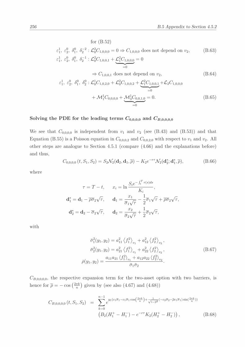
256 B.5 Appendix to Section 4.5.2
for (B.52)
ε11, ε02, δ
01, δ
−22 : L2
0C1,0,0,0 = 0⇒ C1,0,0,0 does not depend on v2, (B.63)
ε11, ε02, δ
01, δ
−12 : L2
0C1,0,0,1 + L21C1,0,0,0︸ ︷︷ ︸
=0
= 0
⇒ C1,0,0,1 does not depend on v2, (B.64)
ε11, ε02, δ
01, δ
02 : L1
0C1,0,2,0 + L20C1,0,0,2 + L2
1C1,0,0,1︸ ︷︷ ︸
=0
+L2C1,0,0,0
+M11C0,0,0,0 +M1
3C0,0,1,0︸ ︷︷ ︸
=0
= 0. (B.65)
Solving the PDE for the leading terms C0,0,0,0 and CB,0,0,0,0
We see that C0,0,0,0 is independent from v1 and v2 (see (B.43) and (B.53)) and that
Equation (B.55) is a Poisson equation in C0,0,0,2 and C0,0,2,0 with respect to v1 and v2. All
other steps are analogue to Section 4.5.1 (compare (4.66) and the explanations before)
and thus,
C0,0,0,0 (t, S1, S2) = S2N2(d2,d1, ρ)−K2e−rτN2(d
∗2;d
∗1, ρ), (B.66)
where
τ = T − t, xi = lnSie
−∫ Tt
r(s)ds
Ki
,
d∗1 = d1 − ρσ2
√τ , d1 =
x1σ1
√τ− 1
2σ1
√τ + ρσ2
√τ ,
d∗2 = d2 − σ2
√τ , d2 =
x2σ2
√τ+
1
2σ2
√τ ,
with
σ21(y1, y2) = a211
⟨f 21
⟩
v1+ a212
⟨f 22
⟩
v2,
σ22(y1, y2) = a221
⟨f 21
⟩
v1+ a222
⟨f 22
⟩
v2, (B.67)
ρ(y1, y2) =a11a21 〈f 2
1 〉v1 + a12a22 〈f 22 〉v2
σ1σ2.
CB,0,0,0,0, the respective expansion term for the two-asset option with two barriers, is
hence for ρ = − cos(2πkn
)given by (see also (4.67) and (4.68))
CB,0,0,0,0 (t, S1, S2) =n−1∑
k=0
ey1(c1σ1−c1σ1 cos( 2πk
n )+ 1√1−ρ2
(−c2σ2−ρc1σ1) sin(2πkn
))
(B2(H
+1 −H−
1 )− e−rτK2(H+2 −H−
2 )), (B.68)
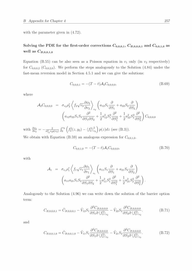
B Appendix for Chapter 4 257
with the parameter given in (4.72).
Solving the PDE for the first-order corrections C0,0,0,1, CB,0,0,0,1 and C0,0,1,0 as
well as CB,0,0,1,0
Equation (B.55) can be also seen as a Poisson equation in v1 only (in v2 respectively)
for C0,0,0,2 (C0,0,2,0). We perform the steps analogously to the Solution (4.84) under the
fast-mean reversion model in Section 4.5.1 and we can give the solutions:
C0,0,0,1 = −(T − t)A2C0,0,0,0, (B.69)
where
A2C0,0,0,0 = σv2ρv2
⟨
f2√v2∂φ2
∂v2
⟩
v2
(
a12S1∂
∂S1
+ a22S2∂
∂S2
)
(
a12a22S1S2∂2
∂S1∂S2
+1
2a212S
21
∂2
∂S21
+1
2a222S
22
∂2
∂S22
)
C0,0,0,0
with ∂φ2
∂v2= − 2
σ2v2
v2p(v2)
∫ v2
0
(
f 22 (z, y2)− 〈f 2
2 〉2v2
)
p(z)dz (see (B.3)).
We obtain with Equation (B.59) an analogous expression for C0,0,1,0.
C0,0,1,0 = −(T − t)A1C0,0,0,0, (B.70)
with
A1 = σv1ρv1
⟨
f1√v1∂φ1
∂v1
⟩
v1
(
a11S1∂
∂S1
+ a21S2∂
∂S2
)
(
a11a21S1S2∂2
∂S1∂S2
+1
2a211S
21
∂2
∂S21
+1
2a221S
22
∂2
∂S22
)
.
Analogously to the Solution (4.96) we can write down the solution of the barrier option
term:
CB,0,0,0,1 = CB,0,0,0,1 − V12S1∂2CB,0,0,0,0
∂S1∂ 〈f 22 〉v2− V22S2
∂2CB,0,0,0,0
∂S2∂ 〈f 22 〉v2
. (B.71)
and
CB,0,0,1,0 = CB,0,0,1,0 − V11S1∂2CB,0,0,0,0
∂S1∂ 〈f 22 〉v2− V21S2
∂2CB,0,0,0,0
∂S2∂ 〈f 22 〉v2
. (B.72)
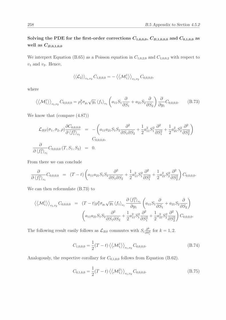
258 B.5 Appendix to Section 4.5.2
Solving the PDE for the first-order corrections C1,0,0,0, CB,1,0,0,0 and C0,1,0,0 as
well as CB,0,1,0,0
We interpret Equation (B.65) as a Poisson equation in C1,0,2,0 and C1,0,0,2 with respect to
v1 and v2. Hence,
〈〈L2〉〉v1,v2 C1,0,0,0 = −⟨⟨M1
1
⟩⟩
v1,v2C0,0,0,0,
where
⟨⟨M1
1
⟩⟩
v1,v2C0,0,0,0 = ρy1σy1
√y1 〈f1〉v1
(
a11S1∂
∂S1
+ a21S2∂
∂S2
)∂
∂y1C0,0,0,0. (B.73)
We know that (compare (4.87))
LBS(σ1, σ2, ρ)∂C0,0,0,0
∂ 〈f 21 〉v1
= −(
a11a21S1S2∂2
∂S1∂S2
+1
2a211S
21
∂2
∂S21
+1
2a221S
22
∂2
∂S22
)
C0,0,0,0,
∂
∂ 〈f 21 〉v1
C0,0,0,0 (T, S1, S2) = 0.
From there we can conclude
∂
∂ 〈f 21 〉v1
C0,0,0,0 = (T − t)(
a11a21S1S2∂2
∂S1∂S2
+1
2a211S
21
∂2
∂S21
+1
2a221S
22
∂2
∂S22
)
C0,0,0,0.
We can then reformulate (B.73) to
⟨⟨M1
1
⟩⟩
v1,v2C0,0,0,0 = (T − t)ρy1σy1
√y1 〈f1〉v1
∂ 〈f 21 〉v1
∂y1
(
a11S1∂
∂S1
+ a21S2∂
∂S2
)
(
a11a21S1S2∂2
∂S1∂S2
+1
2a211S
21
∂2
∂S21
+1
2a221S
22
∂2
∂S22
)
C0,0,0,0.
The following result easily follows as LBS commutes with Si∂k
∂Ski
for k = 1, 2.
C1,0,0,0 =1
2(T − t)
⟨⟨M1
1
⟩⟩
v1,v2C0,0,0,0. (B.74)
Analogously, the respective corollary for C0,1,0,0 follows from Equation (B.62).
C0,1,0,0 =1
2(T − t)
⟨⟨M2
1
⟩⟩
v1,v2C0,0,0,0. (B.75)
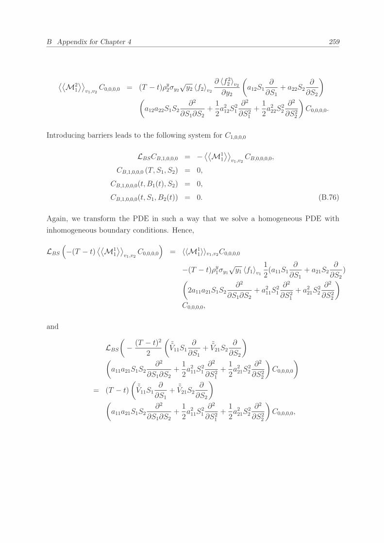
B Appendix for Chapter 4 259
⟨⟨M2
1
⟩⟩
v1,v2C0,0,0,0 = (T − t)ρy2σy2
√y2 〈f2〉v2
∂ 〈f 22 〉v2
∂y2
(
a12S1∂
∂S1
+ a22S2∂
∂S2
)
(
a12a22S1S2∂2
∂S1∂S2
+1
2a212S
21
∂2
∂S21
+1
2a222S
22
∂2
∂S22
)
C0,0,0,0.
Introducing barriers leads to the following system for C1,0,0,0
LBSCB,1,0,0,0 = −⟨⟨M1
1
⟩⟩
v1,v2CB,0,0,0,0,
CB,1,0,0,0 (T, S1, S2) = 0,
CB,1,0,0,0(t, B1(t), S2) = 0,
CB,1,0,0,0(t, S1, B2(t)) = 0. (B.76)
Again, we transform the PDE in such a way that we solve a homogeneous PDE with
inhomogeneous boundary conditions. Hence,
LBS
(
−(T − t)⟨⟨M1
1
⟩⟩
v1,v2C0,0,0,0
)
= 〈〈M11〉〉v1,v2C0,0,0,0
−(T − t)ρy1σy1√y1 〈f1〉v1
1
2(a11S1
∂
∂S1
+ a21S2∂
∂S2
)(
2a11a21S1S2∂2
∂S1∂S2
+ a211S21
∂2
∂S21
+ a221S22
∂2
∂S22
)
C0,0,0,0,
and
LBS
(
− (T − t)22
(
˜V11S1∂
∂S1
+ ˜V21S2∂
∂S2
)
(
a11a21S1S2∂2
∂S1∂S2
+1
2a211S
21
∂2
∂S21
+1
2a221S
22
∂2
∂S22
)
C0,0,0,0
)
= (T − t)(
˜V11S1∂
∂S1
+ ˜V21S2∂
∂S2
)
(
a11a21S1S2∂2
∂S1∂S2
+1
2a211S
21
∂2
∂S21
+1
2a221S
22
∂2
∂S22
)
C0,0,0,0,
260 B.5 Appendix to Section 4.5.2
as LBS commutes with Si∂k
∂Ski
, k = 1, 2 and LBSC0,0,0,0 = 0. Thus, we define
CB,1,0,0,0 = CB,1,0,0,0 − (T − t)⟨⟨M1
1
⟩⟩
v1,v2C0,0,0,0 −
(T − t)22
(
˜V11S1∂
∂S1
+ ˜V21S2∂
∂S2
)
(
a11a21S1S2∂2
∂S1∂S2
+1
2a211S
21
∂2
∂S21
+1
2a221S
22
∂2
∂S22
)
C0,0,0,0,
˜V11 = a11ρy1σy1√y1 〈f1〉v1
∂ 〈f1〉v1∂y1
,
˜V21 = a11ρy1σy1√y1 〈f1〉v1
∂ 〈f1〉v1∂y1
. (B.77)
Hence, we obtain
LBS(ρ, σ1, σ2)CB,1,0,0,0 = 0,
CB,1,0,0,0 (T, S1, S2) = 0,
CB,1,0,0,0(t, B1(t), S2) = ˜g11(t, B1, S2, y1, y2),
CB,1,0,0,0(t, S1, B2(t)) = ˜g12(t, S1, B2, y1, y2), (B.78)
with
˜g11(t, B1, S2, y1, y2) = −(T − t)⟨⟨M1
1
⟩⟩
v1,v2C0,0,0,0
−(T − t)22
(
˜V11S1∂
∂S1
+ ˜V21S2∂
∂S2
)
(
a11a21S1S2∂2
∂S1∂S2
+1
2a211S
21
∂2
∂S21
+1
2a221S
22
∂2
∂S22
)
C0,0,0,0
∣∣S1=B1(ι1),
˜g12(t, S1, B2, y1, y2) = −(T − t)⟨⟨M1
1
⟩⟩
v1,v2C0,0,0,0
−(T − t)22
(
˜V11S1∂
∂S1
+ ˜V21S2∂
∂S2
)
(
a11a21S1S2∂2
∂S1∂S2
+1
2a211S
21
∂2
∂S21
+1
2a221S
22
∂2
∂S22
)
C0,0,0,0
∣∣S2=B2(ι2).
For the solution it holds
CB,1,0,0,0(t, S1, S2, B1, B2) =
∫ T
0
∫ ∞
0
e−c1b1−c2b2e−c2(σ2a′p sinβp)˜g11(t
′, B1, B2eσ2a
′p sin βp)
pxGBM
(ι′ ∈ dt′, θ′p = βp
)da′pdt
′
+
∫ T
0
∫ ∞
0
e−c1b1−c2b2e−c1(σ1a′p
√1−ρ2)˜g21(t
′, B1eσ1
√1−ρ2a′p , B2)
pxGBM
(ι′ ∈ dt′, θ′p = 0
)da′pdt
′. (B.79)
B Appendix for Chapter 4 261
CB,1,0,0,0 is given by
CB,1,0,0,0 = CB1,0,0,0 + (T − t)
⟨⟨M1
1
⟩⟩
v1,v2C0,0,0,0 +
(T − t)22
(
˜V11S1∂
∂S1
+ ˜V21S2∂
∂S2
)
(
a11a21S1S2∂2
∂S1∂S2
+1
2a211S
21
∂2
∂S21
+1
2a221S
22
∂2
∂S22
)
C0,0,0,0. (B.80)
Analogously, we can conclude
CB,0,1,0,0(t, S1, S2, B1, B2) =
∫ T
0
∫ ∞
0
e−c1b1−c2b2e−c2(σ2a′p sinβp)˜g21(t
′, B1, B2eσ2a
′p sin βp)
pxGBM
(ι′ ∈ dt′, θ′p = βp
)da′pdt
′
+
∫ T
0
∫ ∞
0
e−c1b1−c2b2e−c1(σ1a′p
√1−ρ2)˜g22(t
′, B1eσ1
√1−ρ2a′p , B2)
pxGBM
(ι′ ∈ dt′, θ′p = 0
)da′pdt
′, (B.81)
with
˜g21(t, B1, S2, y1, y2) = (T − t)⟨⟨M2
1
⟩⟩
v1,v2C0,0,0,0
−(T − t)22
(
˜V12S1∂
∂S1
+ ˜V22S2∂
∂S2
)
(
a12a22S1S2∂2
∂S1∂S2
+1
2a212S
21
∂2
∂S21
+1
2a222S
22
∂2
∂S22
)
C0,0,0,0
∣∣S1=B1(ι1),
˜g22(t, S1, B2, y1, y2) = −(T − t)⟨⟨M2
1
⟩⟩
v1,v2C0,0,0,0 −
(T − t)22
(
˜V12S1∂
∂S1
+ ˜V22S2∂
∂S2
)
(
a12a22S1S2∂2
∂S1∂S2
+1
2a212S
21
∂2
∂S21
+1
2a222S
22
∂2
∂S22
)
C0,0,0,0
∣∣S2=B2(ι2),
˜V22 = a22ρy2σy2y2 〈f1〉v2
∂σ2∂y2
,
˜V12 = a12ρy2σy2y2 〈f1〉v2
∂σ2∂y2
.
CB,0,1,0,0 is given by
CB,0,1,0,0 = CB0,1,0,0 +
(T − t)22
(
˜V12S1∂
∂S1
+ V22S2∂
∂S2
)
(
a12a22S1S2∂2
∂S1∂S2
+1
2a212S
21
∂2
∂S21
+1
2a222S
22
∂2
∂S22
)
CB,0,0,0,0
+(T − t)〈〈M21〉〉v1,v2C0,0,0,0. (B.82)


List of Symbols
1 . . . . . . . . . . . . . . . . . . . . . . . . Indicator function
A∗f . . . . . . . . . . . . . . . . . . . . . Operator of Kolmogorov forward equation
Af . . . . . . . . . . . . . . . . . . . . . . Infinitesimal generator
A . . . . . . . . . . . . . . . . . . . . . . . Set
AH . . . . . . . . . . . . . . . . . . . . . . Parameter of Heston-type characteristic function
AS2 . . . . . . . . . . . . . . . . . . . . . Parameter of Stein and Stein-type characteristic function
(aij) . . . . . . . . . . . . . . . . . . . . . Matrix of eigenvectors
αdi . . . . . . . . . . . . . . . . . . . . . . . Damping parameter
αk . . . . . . . . . . . . . . . . . . . . . . . kth algebraic moment
a . . . . . . . . . . . . . . . . . . . . . . . . Real number
B (R) . . . . . . . . . . . . . . . . . . . . Borel sigma-algebra
BH . . . . . . . . . . . . . . . . . . . . . . Parameter of Heston-type characteristic function
Bi(t) . . . . . . . . . . . . . . . . . . . . Time-dependant barrier on stock i
BS2 . . . . . . . . . . . . . . . . . . . . . Parameter of Stein and Stein-type characteristic function
βk . . . . . . . . . . . . . . . . . . . . . . . kth geometric moment
βp . . . . . . . . . . . . . . . . . . . . . . . tan−1
(
−√
1−ρ2
ρ
)
b . . . . . . . . . . . . . . . . . . . . . . . . Real number
C . . . . . . . . . . . . . . . . . . . . . . . Complex numbers
Ck . . . . . . . . . . . . . . . . . . . . . . Collection of functions with continuous derivatives up to order
k
Ck0 . . . . . . . . . . . . . . . . . . . . . . Subset of Ck of functions having compact support
CD . . . . . . . . . . . . . . . . . . . . . . Defaultable derivative
CB(t, S1, S2, B1, B2) . . . . . . Barrier option
CDS (t, S1, S2) . . . . . . . . . . . . . Defaultable investment in a stock
CZ(t) . . . . . . . . . . . . . . . . . . . . Zero coupon bond
C1D(t, S1, S2, B2) . . . . . . . . Double-digital single-barrier option
C1P (t, S2, K2, B2) . . . . . . . Knock-out put option
C2C(t, S1, S2, B1, B2) . . . . . Correlation barrier option
C2C(t, S1, S2, B2) . . . . . . . . Correlation single-barrier option

264 LIST OF SYMBOLS
C2D(t, S1, S2, B1, B2) . . . . . Double-digital barrier option
CCall (t, S2, K2) . . . . . . . . . . Call option
CD (t, S2, K2) . . . . . . . . . . . . Digital option
CS2 . . . . . . . . . . . . . . . . . . . . . . Parameter of Stein and Stein-type characteristic function
CIR . . . . . . . . . . . . . . . . . . . . . Cox-Ingersoll-Ross model
χ . . . . . . . . . . . . . . . . . . . . . . . . Probability measure
c . . . . . . . . . . . . . . . . . . . . . . . . Constant
ci . . . . . . . . . . . . . . . . . . . . . . . . Constant
c . . . . . . . . . . . . . . . . . . . . . . . . Constant
c1 . . . . . . . . . . . . . . . . . . . . . . . σ1−σ2ρ
2σ1(1−ρ2)
c2 . . . . . . . . . . . . . . . . . . . . . . . σ2−σ1ρ
2σ2(1−ρ2)
Di(t) . . . . . . . . . . . . . . . . . . . . total debt per share of firm i
D . . . . . . . . . . . . . . . . . . . . . . . Open set
Def(z) . . . . . . . . . . . . . . . . . . . Space in which the moment generating function exists
∂D . . . . . . . . . . . . . . . . . . . . . . Boundary region of D
D . . . . . . . . . . . . . . . . . . . . . . . Bounded region
δj . . . . . . . . . . . . . . . . . . . . . . . Fast mean-reversion speed
d(u) . . . . . . . . . . . . . . . . . . . . .
√
κ2 + σ2v
(
u2 +σ21+σ2
2−2ρσ1σ2
4(1−ρ2)
)
di . . . . . . . . . . . . . . . . . . . . . . . Dividend yield of company i
E [X] . . . . . . . . . . . . . . . . . . . . Expected value of X
E (x) . . . . . . . . . . . . . . . . . . . . Exponential martingale of x
ǫj . . . . . . . . . . . . . . . . . . . . . . . Slow mean-reversion speed
F . . . . . . . . . . . . . . . . . . . . . . . σ-Algebra
(F1 ∗ F2)(y) . . . . . . . . . . . . . Convolution of F1 and F2
F . . . . . . . . . . . . . . . . . . . . . . . . Filtration
Φ . . . . . . . . . . . . . . . . . . . . . . . . Set
F (x) = Q(X ≤ x) . . . . . . . Distribution function of X
f(u) . . . . . . . . . . . . . . . . . . . . . Fourier transform of f(x)
f . . . . . . . . . . . . . . . . . . . . . . . . Complex conjugate of f
ϕ(u) . . . . . . . . . . . . . . . . . . . . . Characteristic function
ϕH . . . . . . . . . . . . . . . . . . . . . . Heston-type characteristic function
ϕGBM . . . . . . . . . . . . . . . . . . . Characteristic function of geometric Brownian motion model
ϕS2 . . . . . . . . . . . . . . . . . . . . . . Stein-and Stein-type characteristic function
fd . . . . . . . . . . . . . . . . . . . . . . . Function of the day effect
f e . . . . . . . . . . . . . . . . . . . . . . . Eigenfunction
G (t,x) . . . . . . . . . . . . . . . . . . Kernel, e.g. fundamental solution, Green function
GF (t, x) . . . . . . . . . . . . . . . . . Free space Green function

LIST OF SYMBOLS 265
GBM . . . . . . . . . . . . . . . . . . . . Geometric Brownian motion model
γ . . . . . . . . . . . . . . . . . . . . . . . . Stochastic process
g(S1, S2) . . . . . . . . . . . . . . . . . Payoff function dependent on S1 and S2 in T
H(x) . . . . . . . . . . . . . . . . . . . . Function only depending on x
h(x) . . . . . . . . . . . . . . . . . . . . . Fourier transformed payoff function
ℑ(u) . . . . . . . . . . . . . . . . . . . . Imaginary part of u
Iς(ab2c2
) . . . . . . . . . . . . . . . . . . . Modified Bessel function of the first kind
ι . . . . . . . . . . . . . . . . . . . . . . . . Stopping time
j . . . . . . . . . . . . . . . . . . . . . . . . Counter with j ∈ N
K(t,x) . . . . . . . . . . . . . . . . . . . Real-valued function
Ki . . . . . . . . . . . . . . . . . . . . . . . Strike for asset i
κ . . . . . . . . . . . . . . . . . . . . . . . . Constant mean-reversion speed
k . . . . . . . . . . . . . . . . . . . . . . . . Counter with k ∈ N
k . . . . . . . . . . . . . . . . . . . . . . . . Counter with k ∈ N
ki . . . . . . . . . . . . . . . . . . . . . . . lnKi
L1 . . . . . . . . . . . . . . . . . . . . . . . Banach space of Lebesgue integrable functions in Rd
L2 . . . . . . . . . . . . . . . . . . . . . . . Hilbert space of square-integrable functions in Rd
Lf . . . . . . . . . . . . . . . . . . . . . . Operator for differential equation
M(u) . . . . . . . . . . . . . . . . . . . . Moment generating function
M = (M(t))t∈[0,T ] . . . . . . . . Local (Q−) martingale
µ(s) . . . . . . . . . . . . . . . . . . . . . Drift parameter
zk1± . . . . . . . . . . . . . . . . . . . . . rp cos
(2kπn± θp
)
zk2± . . . . . . . . . . . . . . . . . . . . . rp sin
(2kπn± θp
)
N . . . . . . . . . . . . . . . . . . . . . . . Natural number
n . . . . . . . . . . . . . . . . . . . . . . . . Exterior unit normal
n (x) . . . . . . . . . . . . . . . . . . . . Non-negative function
ν . . . . . . . . . . . . . . . . . . . . . . . . Real number
(Ω,F ,Q,F) . . . . . . . . . . . . . Filtered probability space
(Ω,F ,Q) . . . . . . . . . . . . . . . . Probability space
(Ω,F) . . . . . . . . . . . . . . . . . . . Measurable space
o (x) . . . . . . . . . . . . . . . . . . . . Non-negative function
ω . . . . . . . . . . . . . . . . . . . . . . . . Random variable
. . . . . . . . . . . . . . . . . . . . . . . Real variable
P . . . . . . . . . . . . . . . . . . . . . . . Real vector
Ψ . . . . . . . . . . . . . . . . . . . . . . . Bonus payment rate
p . . . . . . . . . . . . . . . . . . . . . . . . Participation rate
ϑ(x, t) . . . . . . . . . . . . . . . . . . . Function
p(x) . . . . . . . . . . . . . . . . . . . . . Density function of x

266 LIST OF SYMBOLS
p . . . . . . . . . . . . . . . . . . . . . . . . Number of considered eigenvectors
Q . . . . . . . . . . . . . . . . . . . . . . . Probability measure
q(τ,x′,x, v) . . . . . . . . . . . . . . Probability density function, integrated over v′
R . . . . . . . . . . . . . . . . . . . . . . . Real numbers
R . . . . . . . . . . . . . . . . . . . . . . . Constant recovery rate
ℜ(x) . . . . . . . . . . . . . . . . . . . . Real part of x
Rǫ,δ . . . . . . . . . . . . . . . . . . . . . Error in the approximation for the regularised problem
ρ . . . . . . . . . . . . . . . . . . . . . . . . Correlation
r(s) . . . . . . . . . . . . . . . . . . . . . Deterministic interest rate
rp . . . . . . . . . . . . . . . . . . . . . . . Polar coordinate, radius
Sϕ . . . . . . . . . . . . . . . . . . . . . . . Space in which ϕ is regular
Sg . . . . . . . . . . . . . . . . . . . . . . . Space, in which the transformed payoff function is Fourier
integrable
Si . . . . . . . . . . . . . . . . . . . . . . . Stock i
Sdi (n) . . . . . . . . . . . . . . . . . . . . Discrete normalised price returns of stock i at time n
√∆t
σi . . . . . . . . . . . . . . . . . . . . . . . Diffusion parameter of stock i
σv . . . . . . . . . . . . . . . . . . . . . . . Diffusion parameter of v
ςi . . . . . . . . . . . . . . . . . . . . . . . . Real number
s . . . . . . . . . . . . . . . . . . . . . . . . Time
θp . . . . . . . . . . . . . . . . . . . . . . . Polar coordinate,angle
T . . . . . . . . . . . . . . . . . . . . . . . . Transformation
T . . . . . . . . . . . . . . . . . . . . . . . Maturity time
T (t) . . . . . . . . . . . . . . . . . . . . . Function only depending on t
t . . . . . . . . . . . . . . . . . . . . . . . . Time
〈u,x〉 . . . . . . . . . . . . . . . . . . . Scalar product
〈u,x〉 . . . . . . . . . . . . . . . . . . . Scalar product
u = w + i . . . . . . . . . . . . . . Complex variable
V d,Nj (k) . . . . . . . . . . . . . . . . . . Variogram function with lag k for eigenvalue j
v . . . . . . . . . . . . . . . . . . . . . . . . Process driving the covariance
Wi . . . . . . . . . . . . . . . . . . . . . . Value of firm i
W = (W (t))t≥0 . . . . . . . . . . Brownian motion
w . . . . . . . . . . . . . . . . . . . . . . . Real variable
(X(t))t≥0 . . . . . . . . . . . . . . . . Process
〈X〉 := 〈X,X〉 . . . . . . . . . . . Quadratic variation process of X
Ξ . . . . . . . . . . . . . . . . . . . . . . . . Constant
ξ(t,x) . . . . . . . . . . . . . . . . . . . Continuous function
xi . . . . . . . . . . . . . . . . . . . . . . . ln
(
Si(t)e∫Tt r(s)ds
Ki
)

LIST OF SYMBOLS 267
x∗1(t) . . . . . . . . . . . . . . . . . . . . ln(
S1+D1(t)D1(t)
)
yi . . . . . . . . . . . . . . . . . . . . . . .x∗i
σi
yj . . . . . . . . . . . . . . . . . . . . . . . Driver of the covariance/correlation
Z = (Z(t))t≥0 . . . . . . . . . . . Brownian motion
ζ . . . . . . . . . . . . . . . . . . . . . . . . Constant mean-reversion level
z1 . . . . . . . . . . . . . . . . . . . . . . . 1√1−ρ2
[x1−b1σ1− ρ(x2−b2
σ2)]
z2 . . . . . . . . . . . . . . . . . . . . . . . x2−b2σ2


List of Tables
3.1 Prices of the two-asset double-digital barrier option computed in the limit
to bivariate normal distribution. . . . . . . . . . . . . . . . . . . . . . . . . 81
3.2 Prices of double-digital options with barriers in Heston-type model (Fourier
technique). . . . . . . . . . . . . . . . . . . . . . . . . . . . . . . . . . . . . 83
3.3 Prices of double-digital options with barriers in Heston-type model (Fourier
technique) with low σ-values. . . . . . . . . . . . . . . . . . . . . . . . . . 83
3.4 Prices of the two-asset barrier correlation option computed in the limit to
bivariate normal distribution. . . . . . . . . . . . . . . . . . . . . . . . . . 90
3.5 Prices of correlation options with barriers barriers in Heston-type model
(Fourier technique). . . . . . . . . . . . . . . . . . . . . . . . . . . . . . . . 92
3.6 Prices of correlation options with barriers in Heston-type model (Fourier
technique) with low σ-values. . . . . . . . . . . . . . . . . . . . . . . . . . 92
3.7 Prices of double-digital options with barriers in Heston-type model (PDE
technique). . . . . . . . . . . . . . . . . . . . . . . . . . . . . . . . . . . . . 109
3.8 Prices of double-digital options with barriers in Heston-type model (PDE
technique). . . . . . . . . . . . . . . . . . . . . . . . . . . . . . . . . . . . . 109
3.9 Prices of double-digital options with barriers in Stein-type model (PDE
technique). . . . . . . . . . . . . . . . . . . . . . . . . . . . . . . . . . . . . 110
3.10 Prices of correlation options with barriers in Heston-type model (PDE tech-
nique). . . . . . . . . . . . . . . . . . . . . . . . . . . . . . . . . . . . . . . 111
3.11 Prices of correlation options with barriers in Heston-type model (PDE tech-
nique). . . . . . . . . . . . . . . . . . . . . . . . . . . . . . . . . . . . . . . 112
3.12 Prices of correlation options with barriers in Stein-type model (PDE tech-
nique). . . . . . . . . . . . . . . . . . . . . . . . . . . . . . . . . . . . . . . 113

270 LIST OF TABLES
4.1 Estimated mean-reverting speeds (κ∗vj , j = 1, 2) and typical times for
mean-reversion ( 1κ∗vj
, j = 1, 2). . . . . . . . . . . . . . . . . . . . . . . . . . 149
4.2 Prices of the two-asset option computed with Fourier technique and ap-
proximation. . . . . . . . . . . . . . . . . . . . . . . . . . . . . . . . . . . . 192
List of Figures
2.1 Strip of analyticity . . . . . . . . . . . . . . . . . . . . . . . . . . . . . . . 25
2.2 Contour variation within strip of regularity . . . . . . . . . . . . . . . . . . 28
2.3 Contour variation with simple poles . . . . . . . . . . . . . . . . . . . . . . 30
3.1 Method of images in a circle (with β = π3). . . . . . . . . . . . . . . . . . . 70
3.2 Double-Digital Option with Barriers (ρ=0). . . . . . . . . . . . . . . . . . 82
3.3 Double-Digital Option with Barriers (ρ=-0.5). . . . . . . . . . . . . . . . . 82
3.4 Contour variation. . . . . . . . . . . . . . . . . . . . . . . . . . . . . . . . 86
3.5 Correlation Option with Barriers (ρ=0). . . . . . . . . . . . . . . . . . . . 90
3.6 Correlation Option with Barriers (ρ=-0.5). . . . . . . . . . . . . . . . . . . 91
3.7 IC: Analysis of issuer risk in GBM framework. . . . . . . . . . . . . . . . . 126
3.8 IC: Impact of σv in stochastic covariance framework. . . . . . . . . . . . . 127
3.9 Default probability: Impact of σv. . . . . . . . . . . . . . . . . . . . . . . . 128
3.10 Default probabilities for σv = 0, 2 and D1(0) = 50, 100. . . . . . . . . . . . 128
3.11 PG: Analysis of issuer risk in GBM framework. . . . . . . . . . . . . . . . 130
3.12 PG: Impact of σv. . . . . . . . . . . . . . . . . . . . . . . . . . . . . . . . . 131
3.13 BG: Analysis of issuer risk in GBM framework. . . . . . . . . . . . . . . . 132
3.14 BG: Impact of σv. . . . . . . . . . . . . . . . . . . . . . . . . . . . . . . . . 133
3.15 DC: Analysis of issuer risk in GBM framework. . . . . . . . . . . . . . . . 134
3.16 DC: Impact of σv. . . . . . . . . . . . . . . . . . . . . . . . . . . . . . . . . 135
3.17 BC: Analysis of issuer risk in GBM framework. . . . . . . . . . . . . . . . 136
3.18 BC: Impact of σv. . . . . . . . . . . . . . . . . . . . . . . . . . . . . . . . . 137

272 LIST OF FIGURES
4.1 Observed data (solid line) and estimated functions (dotted line) for the
systematic intra-day behaviour of variability for the eigenfunction j = 1 in
the left figure and for j = 2 in the right one. . . . . . . . . . . . . . . . . . 146
4.2 Empirical variogram functions (dotted lines) and fitted curves (solid lines)
for the two series of normalised eigenvalues Sd1(n) (top plot) and Sd
2(n)(bottom plot) obtained from the intra-day data analysis for Dell and Apple
without considering the day effect. . . . . . . . . . . . . . . . . . . . . . . 148
4.3 Empirical variograms (dashed lines, i.e. Sd1(n) (thinner dashed line with
higher amplitude), Sd1(n) (thicker dashed graph with lower amplitude))
and the respective fitted curves (thinner solid line is the fit for Sd1(n), the
thicker solid line the respective fit for Sd1(n)) after compensating for the
systematic intra-day variability behaviour, compared to the case without
considering the day effect (dotted and solid lines respectively). . . . . . . 149
4.4 Relative difference between exact result and approximation for two-asset
option without barriers for δj =120. . . . . . . . . . . . . . . . . . . . . . . 191
4.5 Relative difference between exact result and approximation for two-asset
option without barriers for δj =12. . . . . . . . . . . . . . . . . . . . . . . . 192
Bibliography
[1] Abramowitz, M. and Stegun, I. A. (1972). Handbook of Mathematical Functions.
National Bureau of Standard, Washington.
[2] Aguilar, O. and West, M. (2000). Bayesian dynamic factor models and variance matrix
discounting for portfolio allocation. Journal of Business and Economic Statistics, 18,
338–357.
[3] Alexander, C. (2000). A primer on the orthogonal GARCH model. Working Paper.
[4] Alexander, C. (2001). Orthogonal GARCH. In “Mastering Risk Volume 2”, Ed. C.
Alexander, Prentice Hall, New York, pages 21–38.
[5] Andersen, T. G., Bollerslev, T., Diebold, F. X., and Ebens, H. (2001). The distribution
of stock return volatility. Journal of Financial Economics, 61, 43–76.
[6] Arcones, M. (2005). Applied Probability Models. Binghampton, NY. http://www.
math.binghamton.edu/MATH/arcones/450/b0.pdf.
[7] Arfken, G. and Weber, J.-H. (1995). Mathematical methods for physicists. Academic
Press, San Diego, 4th edition.
[8] Bakshi, G. and Madan, D. (2000). Spanning and derivative-security valuation. Journal
of Financial Economics, 55, 205–238.
[9] Ball, A. C. and Torous, W. N. (2000). Stochastic correlation across international stock
markets. Journal of Empirical Finance, 7, 373–388.
[10] Bank for International Settlements - Monetary and Economic Department (2010).
Triennial and semiannual surveys positions in global over-the-counter (OTC) derivatives
markets at end-june 2010.
[11] Barndorff-Nielsen, O. and Stelzer, R. (2004). Absolute moments of generalized hyper-
bolic distributions and approximate scaling of normal inverse gaussian levy-processes.
Working paper.
274 BIBLIOGRAPHY
[12] Bingham, N. H. and Kiesel, R. (2004). Risk-Neutral Valuation. Springer Finance,
London, 2nd edition.
[13] Black, F. and Scholes, M. (1973). The pricing of options and corporate liabilities.
Journal of Political Economy, 81, 637–654.
[14] Bollerslev, T., Engle, R. F., and Wooldridge, J. M. (1988). A capital asset pricing
model with time-varying covariances. The Journal of Political Economy, 96, 116–131.
[15] Borovkov, K. and Novikov, A. (2002). On a new approach to calculating expectations
for option pricing. Journal of Applied Probability, 39, 889–895.
[16] Bouzoubaa, M. and Osseiran, A. (2010). Exotic Options and Hybrids: A Guide to
Structuring, Pricing and Trading. John Wiley & Sons Ltd., Wilshire.
[17] Canabarro, E. and Duffie, D. (2004). Measuring and marking counterparty risk. In
“Asset/Liability Management for Financial Institutions”, Ed. L. Tilman, Institutional
Investor Books.
[18] Carr, P. and Madan, D. (1999). Option valuation using the fast Fourier transform.
The Journal of Computational Finance, 2, 61–73.
[19] Carslaw, H. S. and Jaeger, J. C. (1986). Conduction of heat in solids. Oxford
University Press, Oxford, 2nd edition.
[20] Cherubini, U. and Luciano, E. (2002). Copula vulnerability. RISK, 15, 83–86.
[21] Cherubini, U. and Luciano, E. (2004). Pricing swap credit risk with copulas. EFMA
2004 Basel Meetings Paper.
[22] Chib, S., Nardari, F., and Shephard, N. (2006). Analysis of high dimensional multi-
variate stochastic volatility models. Journal of Econometrics, 134, 341–371.
[23] Christoffersen, P., Heston, S., and Jacobs, K. (2009). The shape and term structure
of the index option smirk: Why multifactor stochastic volatility models work so well.
Management Science, 55, 1914–1932.
[24] Conlon, J. and Sullivan, M. (2005). Convergence to Black–Scholes for ergodic volatil-
ity models. European Journal of Applied Mathematics, 16, 385–409.
[25] Cox, J. C., Ingersoll, J. E., and Ross, S. A. (1985). A theory of the term structure
of interest rates. Econometrica, 53, 385–408.
BIBLIOGRAPHY 275
[26] da Fonseca, J., Grasselli, M., and Tebaldi, C. (2007). Option pricing when corre-
lations are stochastic: an analytical framework. Review of Derivatives Research, 10,
151–180.
[27] da Fonseca, J., Grasselli, M., and Tebaldi, C. (2008). A multifactor volatility Heston
model. Quantitative Finance, 8, 591–604.
[28] Daniels, H. (1982). Sequential tests constructed from images. The Annals of Statis-
tics, 10, 394–400.
[29] Dassiosy, A. and Nagaradjasarmaz, J. (2006). The square-root process and Asian
options. Quantitative Finance, 6, 337–347.
[30] Deelstra, G. and Parker, G. (1995). A covariance equivalent discretisation of the CIR
model. Proceedings of the 5th AFIR International Colloquium, 2, 731–747.
[31] del Bano Rollin, S., Ferreiro-Castillo, A., and Utzet, F. (2009). A new look at the
Heston characteristic function. Working Paper.
[32] Dempster, M. and Hong, S. (2002). Spread option valuation and the fast Fourier
transform. In “Proceedings of the 1st World Congress of the Bachelier Finance Society”,
Eds. H. Geman, D. Madan and S. R. Pliska, Springer, Berlin, pages 203–220.
[33] Dempster, M. and Hong, S. (2004). Managing correlation risk with spread option
models. Working Paper.
[34] Deutscher Derivate Verband (2010). Marktvolumen. http://www.
deutscher-derivate-verband.de/DE/Showpage.aspx?pageID=29.
[35] D’Hulster, K. I. (2001). Wrong way risk. http://www.isda.org/c_and_a/pdf/
RGresserLetter-Sept701.pdf.
[36] Dragulescu, A. A. and Yakovenko, V. M. (2002). Probability of distribution of returns
in the Heston model with stochastic volatility. Quantitative Finance, 2, 443–453.
[37] Dupire, B. (1994). Pricing with a smile. Risk, 7, 18–20.
[38] Eberlein, E., Glau, K., and Papapantoleon, A. (2010). Analysis of Fourier transform
valuation formulas and applications. Applied Mathematical Finance, 17, 211–240.
[39] Einig, K. (2010). Pricing of certificates under issuer risk in a stochastic volatility
model. Diplomarbeit, Centre of Mathematical Sciences, Munich University of Technol-
ogy, Garching bei Munchen.
276 BIBLIOGRAPHY
[40] Engle, R. F. (2002). Dynamic conditional correlation - a simple class of multivariate
GARCH models. Journal of Business and Economic Statistics, 17, 339–350.
[41] Escobar, M. and Olivares, P. (2008). The principal component stochastic volatility
model: Estimation and pricing of mountain range derivatives. Working Paper.
[42] Escobar, M., Gotz, B., and Zagst, R. (2007). Pricing of a CDO on stochastically
correlated underlyings. Working Paper.
[43] Feller, W. (1950). An Introduction to Probability Theory and its Applications, Vol I.
Wiley, New York, 1st edition.
[44] Feller, W. (1951). Two singular diffusion problems. The Annals of Mathematics, 54,
173–182.
[45] Feller, W. (1970). An Introduction to Probability Theory and its Applications, Vol
II. Wiley, New York, 1st edition.
[46] Feng, J., Forde, M., and Fouque, J. (2010). Short maturity asymptotics for a fast
mean reverting Heston stochastic volatility model. SIAM Journal on Financial Math-
ematics, 1, 126–141.
[47] Fouque, J. P., G. P. and Sircar, K. R. (1999). Financial modeling in a fast mean-
reverting stochastic volatility environment. Asia-Pacific Financial Markets, 6, 37–48.
[48] Fouque, J. and Han, C. (2003). Pricing Asian options with stochastic volatility.
Quantitative Finance, 3, 352–362.
[49] Fouque, J., Papanicolaou, G., and Sircar, R. (2000). Derivatives in Financial Markets
with stochastic Volatility. Cambridge University Press, River Edge, NJ., 1st edition.
[50] Fouque, J., Papanicolaou, G., Sircar, R., and Solna, K. (2003a). Multiscale stochastic
volatility asymptotics. SIAM Journal on Multiscale Modeling and Simulation, 2, 22–42.
[51] Fouque, J., Papanicolaou, G., Sircar, R., and Solna, K. (2003b). Short time-scales in
S&P 500 volatility. Journal of Computational Finance, 6, 1–23.
[52] Fouque, J., Papanicolaou, G., Sircar, R., and Solna, K. (2003c). Singular perturba-
tions in option pricing. SIAM Journal on Applied Mathematics, 63, 1648–1665.
[53] Fouque, J., Sircar, R., and Solna, K. (2006). Stochastic volatility effects on default-
able bonds. Applied Mathematical Finance, 13, 215–244.
[54] Fouque, J., Garnier, J., Papanicolaou, G., and Solna, K. (2007). Wave Propagation
and Time Reversal in Randomly Layered Media. Springer, New York, 1st edition.
BIBLIOGRAPHY 277
[55] Fouque, J., Wignall, B., and Zhou, X. (2008). Modeling correlated defaults: First
passage model under stochastic volatility. Journal of Computational Finance, 11, 43–
78.
[56] Gourieroux, C. (2006). Continuous time Wishart process for stochastic risk. Econo-
metric Reviews, 25, 177–217.
[57] Gourieroux, C. and Sufana, R. (2005). Derivative pricing with multivariate stochastic
volatility: Application to credit risk. Conference Paper: Econometric World Congress,
London, UK.
[58] Gourieroux, C., Jasiak, J., and Sufana, R. (2009). The Wishart autogressive process
of multivariate stochastic volatility. Journal of Econometrics, 150, 167–181.
[59] Gradshtein, I. S. and Ryzhik, I. (2000). Table of integrals, series, and products.
Academic Press, San Diego, CA; London.
[60] Harell, E. M. and Herod, J. V. (2000). Linear Methods of Applied Mathematics.
Atlanta, GA. http://www.mathphysics.com/pde/.
[61] Harvey, A., Ruiz, E., and Shephard, N. (1994). Multivariate stochastic covariance
models. Review of Economic Studies, 61, 247–264.
[62] Haug, E. G. (1997). The Complete Guide to Option Pricing Formulas. Mcgraw-Hill
Professional, 1st edition.
[63] Hazewinkel, M. E. (2002). Linear Methods of Applied Mathematics. Springer, Berlin,
Heidelberg, New York. http://eom.springer.de/.
[64] He, H., Keirstead, W., and Rebholz, J. (1998). Double lookbacks. Mathematical
Finance, 8, 201–228.
[65] Heston, S. (1993). A closed-form solution for options with stochastic volatility with
applications to bond and currency options. Journal of Finance, 42, 327–343.
[66] Howison, S. (2005). Matched asymptotic expansions in financial engineering. Journal
of Engineering Mathematics, 53, 385–406.
[67] Hull, J. C. (2002). Options, Futures, and Other Derivatives. Prentice Hall, New
York, 5th edition.
[68] Hull, J. C. and White, A. D. (1987). The pricing of options on assets with stochastic
volatilities. Journal of Finance, 42, 281–300.
278 BIBLIOGRAPHY
[69] Hull, J. C. and White, A. D. (1995). The impact on default risk on the prices of
options and other derivative securities. Journal of Banking and Finance, 19, 299–322.
[70] Ilhan, A., Jonsson, M., and Sircar, R. (2002). Singular perturbations for boundary
value problems arising from exotic options. SIAM Journal of Applied Mathematics, 64,
1268–1293.
[71] Iyengar, S. (1985). Hitting lines with two-dimensional Brownian motion. SIAM
Journal of Applied Mathematics, 45, 983–989.
[72] Jarrow, R. and Turnbull, S. M. (1995). Pricing derivatives on financial securities
subject to credit risk. Journal of Finance, 50, 53–85.
[73] Johnson, H. (1987). Options on the maximum or the minimum of several assets. The
Journal of Financial and Quanitative Analysis, 22, 277–283.
[74] Johnson, H. and Stulz, R. (1987). The pricing of options with default risk. Journal
of Finance, 42, 267–280.
[75] Kallsen, J. (2006). A didactic note on affine stochastic volatility models. In “From
Stochastic Calculus to Mathematical finance”, Eds. Yu. Kabanov, R. Lipster and J.
Stoyanov, Springer, Berlin, pages 343–368.
[76] Karatzas, I. and Shreve, S. E. (1991). Brownian Motion and Stochastic Calculus.
Springer-Verlag, Berlin, 2nd edition.
[77] Kim, S. and Shephard, N. (1998). Stochastic volatility: Likelihood inference and
comparison with ARCH models. The Review of Economic Studies, 65, 361–393.
[78] Klein, P. (1996). Pricing Black-Scholes options with correlated credit risk. Journal
of Banking and Finance, 20, 1211–1229.
[79] Klein, P. and Inglis, M. (2001). Pricing vulnerable European options when the option
payoff can increase the risk of financial distress. Journal of Banking and Finance, 25,
993–1012.
[80] Konigsberger, K. (2003). Analysis 2. Springer Verlag, Berlin.
[81] Lewis, A. L. (2000). Option Valuation under Stochastic Volatility : with Mathematica
Code. Finance Press.
[82] Lewis, A. L. (2001). A simple option formula for general jump-diffusion and other
exponential Levy processes. Working paper.
BIBLIOGRAPHY 279
[83] Lipton, A. (2001). Mathematical Methods for Foreign Exchange: A Financial Engi-
neer’s Approach. World Scientific Publishing Co. Pte. Ltd., Singapore.
[84] Lukacs, E. (1960). Characteristic Functions. Charles Griffin & Company Limited,
London, 1st edition.
[85] Lukacs, E. and Otto, S. (1953). On analytic characteristic functions. Pacific Journal
of Mathematics, 3, 615–625.
[86] Margrabe, W. (1978). The value of an option to exchange one asset for another. The
Journal of Finance, 33, 177–186.
[87] Merton, R. C. (1974). On the pricing of corporate debt: the risk structure of interest
rates. Journal of Finance, 29, 449–470.
[88] Metzler, A. (2009). On the first passage problem for correlated Brownian motion.
Statistics and Probability Letters, doi:10.1016/j.spl.2009.11.001.
[89] Muhle-Karbe, J., Pfaffel, O., and Stelzer, R. (2010). Option pricing in multivariate
stochastic volatility models of OU type. Working paper.
[90] Neykova, D. (2011). Derivatives Pricing under Stochastic Covariance with a Fast
and a Slow Mean-reverting Component - A Perturbation Theory Approach. Diplomar-
beit, Centre of Mathematical Sciences, Munich University of Technology, Garching bei
Munchen.
[91] Øksendal, B. (2003). Stochastic Differential Equations. Springer-Verlag, Berlin, 6th
edition.
[92] Philipov, A. and Glickman, M. E. (2006). Multivariate stochastic volatility via
Wishart processes. Journal of Business and Economic Statistics, 24, 313–328.
[93] Pigorsch, C. and Stelzer, R. (2009). A multivariate Ornstein-Uhlenbeck type stochas-
tic volatility model. Working paper.
[94] Pitt, N. and Shephard, N. (1999). Time-varying covariances: A factor stochastic
volatility approach. Bayesian Statistics, 6, 547–570.
[95] Pooley, D., Forsyth, P., Vetzal, K., and Simpson, R. (2000). Unstructured meshing
for two asset barrier options. Applied Mathematical Finance, 7, 33–60.
[96] Pratt, W. K. (2001). Digital Image Processing: PIKS Inside. John Wiley & Sons
Ltd.
280 BIBLIOGRAPHY
[97] Pykhtin, M. and Zhu, S. (2006). Measuring counterparty credit risk for trading
products under Basel II. In “Basel II Handbook: A Guide for Financial Practitioners
(2nd edition)”, Eds. M. Ong, Risk Books.
[98] Pykhtin, M. and Zhu, S. (2007). A guide to modeling counterparty credit risk. GARP
Risk Review.
[99] Ramachand, L. and Susmel, R. (1998). Volatility and cross-correlation across major
stock markets. Journal of Empirical Finance, 5, 397–416.
[100] Range, M. (2003). Complex analysis: A brief tour into higher dimensions. Amer.
Math. Monthly, 110, 89 – 108.
[101] Rasmussen, H. and Wilmott, P. (2002). Asymptotic analysis of stochastic volatility
models. In “New Directions in Mathematical Finance”, Eds. P. Wilmott and H. O.
Rasmussen, Wiley.
[102] Reed, M. and Barry, S. (1980). Functional Analysis, Volume I. Academic Press,
San Diego, CA., 1st edition.
[103] Romano, M. and Touzi, N. (1997). Contingent claims and market completeness in
a stochastic volatility model. Mathematical Finance, 7, 399–410.
[104] Schmelzle, M. (2010). Option pricing formulae using Fourier transform: Theory and
application. Working Paper.
[105] Schobel, R. and Zhou, J. (1999). Stochastic volatility with an Ornstein-Uhlenbeck
process: An extension. European Finance Review, 3, 23–46.
[106] Scott, L. (1987). Option pricing when the variance changes randomly: Theory,
estimation and an application. Journal of Financial and Quantitative Analysis, 22,
419–438.
[107] Sepp, A. (2006). Extended CreditGrades model with stochastic volatility and jumps.
Wilmott Magazine, 54, 50–62.
[108] Skintzi, V. and Refenes, A.-P. (2005). Implied correlation index: A new measure of
diversification. Journal of Futures Markets, 25, 171–197.
[109] Sommerfeld, A. (1894). Zur analytischen Theorie der Warmeleitung. Math. Ann.,
45, 263–277.
[110] Stamicar, R. and Finger, C. (2005). Incorporating equity derivatives into the Cred-
itGrades model. RiskMetrics Group.
BIBLIOGRAPHY 281
[111] Stein, E. M. and Stein, J. C. (1991). Stock price distributions with stochastic
volatility: an analytic approach. The Review of Financial Studies, 4, 727–752.
[112] Stulz, R. (1982). Options on the minimum or the maximum of two risky assets.
Journal of Financial Economics, 33, 161–185.
[113] Titchmarsh, E. (1948). Introduction to the Theory of Fourier Integrals. Oxford
University Press, London.
[114] van Emmerich, C. (2006). Modelling correlation as a stochastic process. Working
paper, Preprint BUW-AMNA 06/03.
[115] Vasicek, O. (1977). An equilibrium characterization of the term structure. Journal
of Financial Economics, 5, 1569–1622.
[116] Walmsley, J. (1997). New financial instruments. John Wiley & Sons, Inc., 2nd
edition.
[117] Walters, P. (2000). An introduction to Ergodic Theory. Springer, New York, 1st
softcover printing edition.
[118] Wiggins, J. (1987). Option values under stochastic volatility: theory and empirical
estimates. Journal of Financial Economics, 19, 351–372.
[119] Zagst, R. (2002). Interest rate management. Springer-Verlag, Berlin, 1st edition.
[120] Zagst, R. and Huber, M. (2009). Zertifikate spielend beherrschen. FinanzBuch
Verlag GmbH, Munchen, 1st edition.
[121] Zauderer, E. (2006). Partial Differential Equations of Applied Mathematics. John
Wiley & Sons, Inc., New Jersey.
[122] Zhang, P. (1998). Exotic Options. World Scientific Publishing, Cambridge, 2nd
edition.
[123] Zhou, C. (1997). Default correlation: An analytical result. Technical report, Federal
Reserve Board.
[124] Zhou, C. (2001). An analysis of default correlations and multiple defaults. Review
of Financial Studies, 14, 555–576.
[125] Zumbach, G. (2009). The empirical properties of large covariance matrices. Working
Paper.