VALUE-BASED MULTIDISCIPLINARY TECHNIQUES FOR

COMMERCIAL AIRCRAFT SYSTEM DESIGN

Jacob Markish*

Charles River Associates

Karen Willcox†

Massachusetts Institute of Technology

ABSTRACT

A quantitative tool is presented to perform program-level valuation of commercial aircraft

designs. The algorithm used expands upon traditional net present value methods through the

explicit consideration of market uncertainty and the ability of the firm to react to such

uncertainty through real-time decision-making throughout the course of the aircraft program.

The algorithm links three separate models—performance, cost, and revenue—into a system-level

analysis by viewing the firm as a decision-making agent facing continuous choices between

several different “operating modes.” An optimization problem is set up and solved using a

dynamic programming approach to find a set of operating mode decisions that maximizes the

firm’s expected value from the aircraft project. The result is a quantification of value that can be

used to make program-level design trades and to gain insight into the effects of uncertainty on a

particular aircraft design. Examples are drawn from the Blended-Wing-Body aircraft concept to

demonstrate the operation of the program valuation tool.

* Consulting Associate, 200 Clarendon St, T-33, Boston, MA 02116.

†Assistant Professor of Aeronautics & Astronautics, Room 37-447, 77 Massachusetts Avenue,

Cambridge, MA 02139, Member AIAA.

1

2

INTRODUCTION

Traditional methods for creating a commercial aircraft program typically consist of at least two

distinct design efforts—the engineering development of the airframe itself, and the strategic

development of the aircraft program. The latter addresses questions like which aircraft designs to

invest in (product mix), how much production to plan for (sales volume), what prices and costs

to expect (profitability), and how to plan for unforeseen market developments (flexibility).

In the past, the above two elements of program design—engineering development and

strategic development—have often been executed entirely separately from each other.

Engineering and finance are often handled by different groups and at different times. By

uncoupling engineering and finance, a firm runs the risk of overlooking important interactions

between the two. A design system that performs engineering and financial analysis

simultaneously may improve upon the efficiency and effectiveness of the traditional methods.

Numerous advances have been made in the application of multidisciplinary techniques to the

engineering facet of aircraft development. The field of multidisciplinary design optimization

(MDO) combines engineering disciplines, such as aerodynamics, structural dynamics and

controls, to provide a design framework that “coherently exploits the synergism of mutually

interacting phenomena”1. MDO has been implemented across a wide range of applications for

aircraft design1,2. While multidisciplinary analysis and optimization has seen extensive use for

technical design problems in aerospace, there has been less emphasis on applying these

techniques to larger scope system design. Frameworks have been developed that include both

engineering and cost elements for aircraft design3,4 and aircraft engine design5,6. A common

feature of those frameworks is that they use Monte Carlo simulation (MCS) to explore the

impact of uncertainty on system design. While MCS provides a means to perform probabilistic

3

analysis of a series of designs, it does not rigorously address the issue of real-time managerial

decision-making. Tools such as real options and game theory have been suggested as a means to

incorporate decision making (see, for example, Ref. 5), but do not appear to have been

implemented as such.

The objective of this paper is to couple engineering and financial design—or, phrased

differently, product and program design—to extract maximum value from the commercial

aircraft design process. A multidisciplinary analysis is synthesized by creating three freestanding

quantitative models - performance, cost and revenue - and linking them to compute a measure of

program value. While the models are not high fidelity, their purpose is to establish a useful

foundation for further study and to gain insight into the interactions between technical and

program design.

In order to link the above three models into an integrated multidisciplinary analysis tool,

consideration must be given to the program structure—i.e., the decision structure affecting

product mix, design and production plans, and pricing strategy. With this element in place, the

stage is set for a quantitative valuation of the program, which enables both technical and

program-based trade studies to search for an optimal system design. This conceptual process is

illustrated in Figure 1. In this work, the valuation will be performed using a dynamic

programming (DP) framework. The DP approach provides a quantitative measure of the

program’s net present value (NPV), while explicitly accounting for the effects of uncertainty and

program flexibility by modeling the program as a series of decisions. This approach has been

explored in finance literature as Real Options (for example, see Ref. 7 and 8). The algorithm

results in a series of decision rules, which define the optimal decision strategy as a function of

4

evolving and uncertain market conditions. This information could not be obtained using a MCS

approach.

The next section summarizes the multidisciplinary approach taken to accomplish the above

objective by describing the three distinct models used to solve the problem: performance, cost,

and revenue estimation. The following section describes the DP approach to link these models

into one program value analysis tool, and two examples are given to demonstrate the operation

of the valuation tool for analysis of a Blended-Wing-Body (BWB) family of aircraft9. Finally,

the results are discussed, and conclusions are drawn.

PERFORMANCE MODEL

The performance estimator is based on the WingMOD aircraft design tool. WingMOD is an

MDO code that optimizes aircraft wings and horizontal tails subject to a wide array of practical

constraints10,11. WingMOD uses low fidelity analyses to quickly analyze an aircraft in over

twenty design conditions that are needed to address issues from performance, aerodynamics,

loads, weights, balance, stability and control. The low computational cost of the simple analyses

allows the examination of all these issues in an optimization with over one hundred design

variables while achieving reasonable computation time.

As detailed in Ref. 10, the WingMOD optimization framework takes a set of constraints

representing mission requirements (range, payload capacity, cruise speed, approach speed,

balance, etc.) and finds an optimal aerodynamic and structural configuration such that the

resulting aircraft satisfies the constraints. In the valuation framework described here, the

performance characteristics of the aircraft were assumed to be fixed – that is, WingMOD was

run a priori to determine the minimum take-off weight aircraft. Certain properties of the resulting

5

design were then used as input to the value framework. These WingMOD outputs are

summarized in Table 1.

Table 1: WingMOD outputs used as an input to the value framework.

Output Description

MTOW (maximum takeoff weight) Gross vehicle weight at start of max. range mission.

DLW (design landing weight) Gross vehicle weight at end of max. range mission.

Design range Maximum range. Specified as a constraint.

Seats Number of passenger seats. Specified as a constraint.

Weight breakdown Estimates of weight for each primary component of the

aircraft, summing to Operating Empty Weight (OEW).

• Structure

o Fuselage bays

o Inner wing

o Outer wing

o Etc…

Structural elements (spars, ribs, skin, etc.).

The structural weight is broken down into a set of large

“parts” which together comprise the airframe.

• Propulsion Engines, nacelles, and supporting equipment.

• Systems Onboard systems, e.g. avionics, fuel, hydraulics..

• Payloads Seats, bag racks, cargo equipment, etc.

6

COST MODEL

The cost model has two components: manufacturing cost and development cost. While detailed

cost models are available publicly, such as the Aircraft Life Cycle Cost Analysis (ALCCA)

code12, for this research, a simple cost model was developed. An important attribute of the cost

model is that it should capture the effect of commonality between several different airframes – in

general, both the development cost and manufacturing cost of a new aircraft will depend upon

the aircraft’s technical parameters and the technical parameters of other aircraft types that have

already been designed or built.

The cost models used for this research are based upon the decomposition of the aircraft into a

set of components. A simple cost per pound estimation is applied at a component level and

further modified with learning curve effects. The cost model parameters were derived from

publicly available data and are published in detail in Refs. 13 and 14. A more detailed cost

model could be linked to the valuation framework, provided commonality effects are captured.

REVENUE MODEL

Given an aircraft design, a production rate, and a time horizon, the revenue model must provide

the following three outputs: potential revenue cashflow for the current time period, the expected

value of future revenue cashflows, and a measure of the uncertainty of the future cashflows.

Further, the model must demonstrate realistic sensitivities to changes in aircraft performance

(e.g., reduction in fuel burn), changes in the aircraft target market (e.g. 100 v. 250 passengers),

and changes in aircraft price charged (i.e., demand price elasticity). To achieve this functionality,

the model development is broken up into a static analysis and a dynamic analysis.

Static Demand Analysis

The static analysis estimates a baseline price and corresponding quantity demanded, along

with an expected demand growth rate over the specified time horizon. Price is modeled as a

function of several variables representing an aircraft’s value to its operator, an airline. Several

sets of variables and several functional forms were tested by applying the price model to 23

existing aircraft: 11 narrowbodies and 12 widebodies. The outputs generated by the price model

were compared to best estimates for the actual sale prices for each of the aircraft, compiled from

two sources15,16. For each functional form tested, the function parameters were adjusted to

minimize the mean squared error of estimated price.

The selected functions for narrow-body (NB) and wide-body (WB) aircraft are shown below.

Note that speed (or Mach number) is not one of the variables. No significant statistical

relationship between price and speed was found in the range of available data.

(1.910

0.735 0.427 _ _

Seats RangeSeats ref Range ref

= +

)∆Price NB Price_ref - LC (1)

(2.760

0.508 0.697 _ _

Seats RangeSeats ref Range ref

= +

)∆Price WB Price_ref - LC (2)

where Seats is the passenger capacity, Range is the design range, and Seats_ref, Range_ref and

Price_ref are reference values of 419 seats, 8810 nm and $148.7M respectively. ∆(LC) is an

increment in lifecycle cost due to off-nominal Cash Airplane Related Operating Costs (CAROC),

which are equal to total operating costs less ownership costs. This term refers to the additional

cost the operator incurs if the aircraft’s CAROC is greater than the industry average CAROC for

an aircraft of its size. It is a function of the difference between the aircraft’s CAROC and the

7

8

least squares estimate for the CAROC of an aircraft with the same capacity. The prices generated

by the above functions are compared to the best estimates of the actual aircraft prices in Figure 2.

While the aircraft seat count and range are provided by the outputs of the performance model,

its CAROC must be estimated separately. For the example used in this paper, the assumption is

made that fuel costs for a reference mission (3,000 nm) represent 20% of CAROC. The figure of

20% is based on empirical data for several existing aircraft. Fuel burn is calculated using the

Breguet range equation, and a fuel price of $.65 per gallon is used.

Quantity data is based on three distinct forecasts of quantities of aircraft to be delivered from

2000 through 2019 as released by Boeing,17 Airbus,18 and the Airline Monitor.19 Each forecast

has a different set of aircraft categories which comprise the global airline fleet. All three

forecasts were recast into a single, consistent set of aircraft categories based on aircraft class

(narrowbody or widebody) and seat count. Forecasted deliveries are assumed equivalent with

quantities demanded at current market prices. The results are shown in Figure 3. Depending on

seat category, there is considerable variance between the three forecasts. This reflects differences

in the forecasters’ assumptions, methodology, and to some extent, corporate strategy. Further,

the high variance reflects the high degree of uncertainty regarding future revenue cashflows.

For a given aircraft design, the quantity model proceeds as follows. Assign a given aircraft to

a seat category; compute a 20-year gross demand for that category as the mean of the three

forecasts; assume a market share in that category; compute the 20-year quantity demanded as the

market share multiplied by the 20-year gross demand; compute the current annual quantity

demanded by applying the expected annual demand growth rate. If several designs are

considered for production simultaneously, fractions of seat category demands are assigned to

9

each design, such that total quantity demanded will not exceed the product of market share and

20-year gross demand.

Dynamic Demand Analysis

The dynamic analysis aims to quantify the stochastic behavior of the market for commercial

aircraft. It is observed that quantities of aircraft purchased fluctuate significantly from year to

year, and exhibit some cyclical properties. Thus, given a forecast for year 0, it is impossible to

predict with certainty what the quantity of aircraft demanded will be in year 10. However, based

on historical data, some representative characteristics were found to describe historical aircraft

demand levels as geometric Brownian motions, not unlike stock prices. Therefore, the dynamic

analysis uses an average annual growth rate of 4.43% and an average annual volatility of 45.57%

for typical demand evolution patterns for widebody aircraft.

DYNAMIC PROGRAMMING FORMULATION

The basic problem to be solved may be broken up into three parts: endogenous variables—those

that are internal to the aircraft development process and may be controlled, exogenous

variables—those that are external to the aircraft development process and may not be controlled,

and a statement of the problem objective.

The endogenous variables constitute a set (or “portfolio”) of aircraft designs, any of which the

producing firm may choose to develop and bring to market. To bring a concept to market, the

firm must go through several phases: detail design, tooling and capital investment, testing,

certification, and finally production. Each phase entails some required expenditure of time and

money, and the firm may decide when to execute each phase. Each of the aircraft designs is

defined by a set of component parts (e.g., inner wing, outer wing, fuselage bay, etc.), some of

which may be common across several aircraft.

10

Given that an aircraft design is in production, the evolutions of sale price and quantity

demanded are unaffected by any decisions made by the firm and are thus exogenous variables.

Sale price evolves according to a steady growth rate, while quantity demanded evolves as a

stochastic process, characterized by parameters such as drift rate and volatility. Each period that

an aircraft design is in production, as many units are built and sold as are demanded, up to the

maximum capacity of the plant.

Given the above endogenous and exogenous variables, the objective is to find a set of optimal

decision rules governing which aircraft to design, which aircraft to produce, and when; as a

function of the demand level and the aircraft built to date at any given time. Achieving this goal

will necessarily yield the overall program value, because program value is the objective function

used to find the optimal decision rules.

General Theory

A stochastic DP problem may, in general, be framed in five parts:

1. State variables continuously evolve and completely define the problem at any point in time.

2. Control variables are set at any point in time by the decision-maker, and generally impact the

evolution of the state variables.

3. Randomness. One or more of the state variables is subject to random movements, and as

such, involves a stochastic process.

4. Profit function. The goal of the DP method is to maximize some objective function, in this

case the program value. The value is, in general, a function of certain “profits” incurred

every period. These profits are functions of the state variables.

5. Dynamics represent the set of rules that govern the evolution of the state variables, including

the effects of randomness, the effects of control variables, and any other relationships.

The problem is further defined by a time horizon (which may generally be finite or infinite),

and a sequence of time periods of length ∆t, which together comprise the time horizon. The

objective, then, is to find the optimal vector of control variables as a function of time and state,

such that the total value at the initial time is maximized. Equivalently, the objective may be

stated recursively, as an expression for the value at any time, t, as:

[

++= ++ )(

11),(max)( 11 ttttttutt sFE

russF

t

π ] (3)

where Ft(st) is the value (objective function) at time t and state vector st, πt is the profit in time

period t as a function of the state vector st and the control vector ut, r is some appropriate

discount rate, and Et is the expectation operator, providing in this case the expected value of F at

time t+1, given the state st and control ut at time t. Note that the expectation operation for next

period is affected by the control decision and the state in this period.

The above is known as the Bellman equation, and is based on Bellman’s Principle of

Optimality: “An optimal policy has the property that, whatever the initial action, the remaining

choices constitute an optimal policy with respect to the subproblem starting at the state that

results from the initial actions”7. In other words, given that the optimal value problem is solved

for time t+1 and onward, the action (choice of u) maximizing the sum of this period’s profit

flows and the expected future value is also the optimal action maximizing value for the entire

problem for time t and onward.

The Bellman equation can therefore be solved recursively or, for a finite time horizon,

iteratively. For a time horizon of T, this is done by first considering the end of the horizon, at

time tT. At this point, there are no future states, and no future expected value of F. Therefore, the

optimal control decisions, uT, given the final state, sT, are readily found. This process is repeated

11

12

for all possible final values of the state vector, sT. Next, it is possible to take one step backwards

in time, to t = T - 1. Now, equation (3) may be applied to find the optimal control decisions, uT-1,

because the expectation term, E[…], is easily calculated as the probability-weighted average of

the possible future values of FT. Again, the optimal control values, uT-1, are found for each

possible value of sT-1. At this point, the procedure is repeated by taking another backward

timestep to T – 2, and continuing to iterate until the initial time, t = 0, is reached. Now, F0 is

known for all possible initial values of the state, s0, and it is the optimal solution value.

Specific Application: Operating Modes

It is possible to extend the general DP framework presented above to a specific application

useful for the valuation of projects. The application is centered on the concept of “operating

modes,” and has been demonstrated by several authors to be useful in modeling flexible

manufacturing systems8,20. Much of this description is based upon their work.

Consider a hypothetical factory, which at the beginning of any time period may choose to

produce output A or output B. Let the prices for which it can sell each of the outputs be different

functions of a single random variable, x, so it may be more profitable in some situations to

produce one output than the other. However, each time the factory switches production from A

to B, or vice versa, a switching cost is incurred. Thus, it may not always be optimal to simply

produce whichever output yields the higher profit flow in the current period. If there is a high

probability of a switch back to the other output in the future, it may be preferable to choose the

output with the lower profit this period.

This example lends itself well to the DP formulation. In this case, the control variable ut is the

choice of output, or “operating mode,” for the period beginning at time t: A or B. The state

vector, st, consists of two elements: the random variable, x, and the operating mode from last

period, mt. The operating mode m will have one of two possible values, say 0 or 1, representing

output A and B. Depending on the value of mt, the control variable choice ut may result in

payment of a switching cost. Specifically, the Bellman equation may be re-written for this

example as:

1 11( , ) max ( , ) ( , ) ( , )

1tt t t t t t t t t t t tu

F x m x u I m u E F x ur

π + + = − + +

(4)

Note that the state vector s has been separated into its two components—the random variable x

and last period’s operating mode m. Here, the profit function term from (3) has been replaced by

the difference between a profit flow and I(mt, ut)—the switching cost from mode m to mode u.

This will equal zero if mt = ut and there is in fact no switch made, and will be nonzero otherwise.

Note also that the future value, Ft+1 (for which the expectation is found), is a function of the

future random variable, xt+1, and of the current control decision, ut, because ut will become the

“operating mode from last period,” mt+1, at time t+1. In other words, mt+1 = ut, because as soon as

the control decision (ut) is made, the mode in which next period will be entered (mt+1) is set. As

before, this equation can be solved iteratively by starting at the final time period and working

backwards.

One additional point regarding equation (4) bears discussion: the selection of an appropriate

discount rate, r. This is a nontrivial task; in fact, the selection of a discount rate is traditionally

one of the most difficult and sensitive steps in capital budgeting. For an in-depth discussion of

discounting as it applies to this valuation technique, refer to Ref. 13.

13

14

APPLYING DYNAMIC PROGRAMMING TO THE AIRCRAFT DESIGN PROBLEM

The DP approach described above is adapted here to solve the problem of optimal decision-

making in managing an aircraft program. The aircraft program valuation algorithm is briefly

overviewed here in the context of the five parts that frame a DP problem.

1. State variables. For each new aircraft design being simultaneously considered, two state

variables exist: quantity demanded, which evolves stochastically, and the “operating mode

from last period” (as introduced above) for that aircraft.

2. Control variables. For each aircraft design, one control variable exists: the choice of

operating mode for the current period.

3. Randomness. For each aircraft design, one state variable exists with random characteristics:

the quantity demanded. It evolves from a given initial value as a stochastic process.

4. Profit function. The profit function during each period is the sum of profits associated with

the operating modes for each aircraft, less any switching costs incurred during that period.

For production operating modes, the profits are simply revenues less recurring costs;

however, other modes exist for which the profit functions represent non-recurring costs.

5. Dynamics. There are two types of state variables in this formulation: quantity demanded,

which evolves as a stochastic process; and operating mode, which evolves as dictated by the

control variables (operating mode decisions).

Given the above framework, it is useful to consider the impact of various parameters on

computation time. To iteratively solve the problem as described above, the algorithm must

evaluate each possible combination of control variables for each possible state vector; and it

must repeat this process for each timestep in the problem’s time horizon, starting at the final time

t = T and ending at t = 0. Therefore, at the most general level, computation time scales linearly

15

with the time horizon and exponentially with the number of state variables. The time horizon, as

defined in this application, is 30 years, which is a typical valuation timeframe for an aircraft

program. For purposes of simplicity and computation time constraints, the time period length, ∆t,

was selected to be one year. For the same purposes, the maximum number of aircraft designs to

be simultaneously considered by the algorithm was set to two.

Connection to Operating Modes

Whereas the operating modes introduced earlier were simply modes of production, this

formulation extends the operating mode framework to represent each phase of the lifecycle of an

aircraft program. The purpose of this extension is to model the significant time and investment

required to develop an aircraft, before any sales are made. Therefore, the non-recurring

development process, which may last as many as six years, is represented as a chain of

“operating modes.” Clearly, none of these modes entails a positive profit flow. Rather, each has

some negative “profit” associated with the non-recurring investment for that particular phase of

the aircraft development cycle. The only incentive for the firm, and the optimizer, to enter one of

these modes is the opportunity it creates to switch to the following development mode in the

following period, and so on until the production mode is reached. A graphical representation of

the operating modes for a single aircraft design is shown in Figure 4. The diagram is similar in

concept to a Markov chain, where the arrows represent possible transitions between modes. In

fact, the arrows connecting the modes represent switching costs that are finite—if two modes are

not connected by an arrow, the associated switching cost is infinite.

Mode 0 represents the initial conditions: the firm is waiting to invest. Modes 1 through 3

represent roughly the first half of the development effort, primarily detailed design. Note that

several operating modes are shaded. The shading indicates an infinite cost not to switch to a

16

different mode. In other words, it is impossible to remain in a shaded mode for more than one

period. Thus, once the firm commits to a detail design effort, it is assumed impractical to stop

halfway through. However, it is possible to stop before the second half of development—here,

mostly tooling and capital investment—begins. Once this development stage is initiated, a

capacity choice must be made: a low, medium or high capacity production line. This determines

the maximum demand level that may be satisfied with sales every period. Once the capacity

choice is made, the firm must continue to switch modes annually until it reaches mode 6, 9, or

12, at which point it is ready to enter production. Recall that each time period has a duration of

one year—therefore, if the firm does not wait midway through the development process, an

aircraft design takes six years to bring to market. (The six-year baseline duration may be altered,

as discussed below.) The production modes are 13, 14, and 15, corresponding to a low-,

medium-, and high-capacity line. Note that each mode will produce exactly as many units as

demanded each period, up to a maximum that depends upon the mode. The actual values for

maximum capacity are parameters and easily changed. While in production (or waiting to enter

production), it is possible to invest in additional tooling and expand the capacity of the

production line. However, it is assumed impossible to reduce capacity—that is, the scrapping of

tools has little to no salvage value, due to the high specificity of the tools to their product.

Finally, an abandonment mode exists to model any salvage value associated with permanently

shutting down the program. If the salvage value is positive, the switching costs to enter mode 16

will be negative. The determination of switching costs is based upon the adaptation of the

development cost and manufacturing cost models to the operating mode framework.

The development cost model generates a time profile of the non-recurring expenses

associated with the development of a given new aircraft design. Because of the inclusion of two

17

aircraft designs in the valuation algorithm, the switching cost calculation proceeds as follows for

each of the two aircraft designs. The sequential switching costs from mode 0 through mode 9

(medium production rate) are calculated by discretizing the non-recurring cost time profile into

1-year segments. This discretization is done as a step function of the operating mode of the other

aircraft design: if the other aircraft has not yet been fully developed, the baseline non-recurring

cost profile is used. However, if the other aircraft has already been fully developed, the non-

recurring cost profile is calculated with any commonality effects included. Specifically, if the

aircraft share any common components, the development cost and time are both reduced to

reflect the savings resulting from a pre-existing design. If the commonality effects are significant

enough to result in a cost profile shorter than six years, one or more development modes are

skipped. Finally, once medium capacity development process switching costs have been defined,

the switching costs corresponding to the tooling/capital investment part of the development

process are scaled by a “low capacity” and a “high capacity” scaling factor to find the switching

costs corresponding to the low and high capacity decisions.

As with development cost, to account for two aircraft designs present in the valuation, the

switching costs associated with manufacturing are found for each aircraft as functions of the

operating mode of the other aircraft. Switching costs associated with manufacturing have two

components. The first component is switching from a “ready to produce” mode (6, 9, or 12) into

the corresponding production mode (13, 14, or 15, respectively). The second component is

switching from one production line capacity to another. Both of these components are sometimes

involved in a single switch (e.g., 6 to 14, or 6 to 15); however, they are calculated separately and

simply added together as necessary.

18

The costs of switching production line capacity are calculated as the product of a scaling

factor (which is greater than one and represents the additional costs incurred due to disruption of

a pre-existing production line) and the cumulative difference in cash outflows between the two

development processes associated with the production capacities in question. For example, the

cost to switch from low to medium capacity (involved in either a “6 to 14” switch or a “13 to 14”

switch) equals the difference in total development cost between low capacity development

(3,4,5,6) and medium capacity development (3,7,8,9).

The other component of manufacturing-related switching costs is the initial switch into one of

the three production modes (13, 14, or 15). For any given aircraft, the unit cost will generally fall

as production starts and continues to fall due to the learning curve effect. Eventually, it is

reasonable to assume that unit cost approaches an asymptote and stabilizes at the long-run

marginal cost. To exactly model the effect of the learning curve with DP would be impossible,

because knowledge of unit cost requires a knowledge of how many units have been built to date.

This information is not part of the state vector - one possibility would be to include units built to

date as an additional state variable, but because computation time grows exponentially with the

number of state variables as noted above, the exercise would be impractical for even two aircraft.

Therefore, once in a production mode, all aircraft are assumed to be produced at their long-run

marginal cost.

To account for this discrepancy, the switching cost to enter production is set equal to the total

extra cost expected to be incurred during the production run of the aircraft over and above the

long-run marginal cost. Because this extra cost will be incurred gradually and with certainty over

time, the risk-free rate is used to find the expected present value of these cash flows, assuming a

production rate equal to baseline demand.

19

The entire above process, for both development cost and manufacturing cost, is conducted for

both aircraft designs, resulting in a set of switching costs for each that is a function of the

operating mode of the other. To use the symbology introduced earlier, the process finds the

switching costs I(mi, ui | mj) for each aircraft i, where the “other” aircraft is j, for each prior

operating mode mi and control variable decision ui. Then, the switching cost from any operating

mode vector [m1, m2] to [u1, u2] is simply equal to the sum of I(m1, u1 | m2) and I(m2, u2 | m1).

This set of data is stored in the switching cost matrix.

Stochastic Process Dynamics

A crucial component of the algorithm is the model describing the nature of the unpredictable

behavior of the stochastic process representing the development of the market for commercial

aircraft. The annual quantity demanded is represented as a stochastic variable that evolves

according to a random walk, modeled as a binomial tree process. Each time period, the variable

may either increase or decrease by a specified amount with a certain associated probability.

Thus, if there are two such variables, representing the evolution of the market for two distinct

aircraft, there are four possible outcomes each time period. A transition probability matrix is

constructed linking possible initial states to final states in this framework. These transition

probabilities are used to find the expected future value of the project as a probability-weighted

average, expressed as the expectation term E[…] in equation (4).

EXAMPLES

The examples presented here illustrate the mechanics of the algorithm and highlight its

distinguishing features. The first considers design of a single aircraft and presents two

illustrations: a simulation run to demonstrate the decision rules arrived at by the optimizer and a

connection to the NPV technique. The second example considers the design of a family of two

20

aircraft sharing common components and demonstrates how the tool can be used to determine

the value of commonality.

Three different aircraft designs are used, all based upon the BWB concept. Table 2

summarizes the key characteristics of the designs. The example designs are purely hypothetical

and significantly simplified. They do not represent actual current Blended-Wing-Body

configurations. Three different airframes are possible: one large, 747-class vehicle (BWB-450),

and two smaller, 250-passenger class designs. One of the smaller designs, the BWB-250C shares

39.7% of its parts, by weight, with the BWB-450. The other has no commonality with the BWB-

450, being a point design, optimized without consideration for commonality. Note that the point

design results in a lighter airframe, because the commonality constraint placed upon the BWB-

250C results in a weight penalty. Specifically, the BWB-250C uses the same wing as the BWB-

450 to save on development cost, but an individually optimized design for the BWB-250 would

not need as much wing area.

Table 2. BWB example key characteristics.

Design Seat Count Range (nm) GTOW (normalized) Commonality (by weight)

BWB-450 475 8550 1 N/A

BWB-250C 272 8550 0.756 39.7%

BWB-250P 272 8550 0.624 0%

Single Aircraft Valuation

The DP algorithm was applied for valuation of the BWB-250C, resulting in a set of decision

rules, which are shown in Figure 5. These decision rules represent the optimal decision strategy

identified by the algorithm. For each control variable (in this case, there is only one—the next

21

period operating mode decision), the decision rules specify the optimal value to which the

variable should be set, as a function of time and of all the state variables. In other words, given

how long the program has been ongoing, the operating mode from last period, and the current

market conditions (quantity demanded), the decision rule specifies what the operating mode

should be for the next period. Figure 5 shows, as a function of time, the minimum value of the

demand index for which it is optimal to make certain program-related decisions—namely: wait;

design (enter mode 1 from mode 0); build (enter mode 13, 14, or 15 from mode 6, 9, or 12);

switch from low- to medium-capacity production (enter 14 from 13); and switch from low- to

high-capacity production (enter 15 from 13).

Figure 6 shows a simulation run, which represents a sample path of demand through time—a

scenario constructed using a random number generator to approximate the stochastic behavior of

demand. The upper half of the figure plots the random evolution of annual quantity demanded

over time: this is a sample path of the underlying stochastic process. On the same plot is the

optimizer’s real-time strategy in response to the evolution of demand using the decision rules

shown in Figure 5. Thus, at the beginning of the simulation, demand is at its baseline static

forecast quantity, as calculated by the revenue model. This demand level, which happens to be

28 units per year, is insufficient for the firm to commit to developing the BWB (according to the

optimal strategy). However, in year 3, demand increases as the result of a random fluctuation,

and the choice is made to invest in non-recurring development for the aircraft. The investment

choice is made because the new level of demand is greater than the threshold level

corresponding to the “design” decision at time t=3 in the optimizer’s solution. Recall that once

the initial “design” operating mode is entered, the firm is committed to the first phase of the

development process, until halfway through development, immediately before tooling. In this

22

simulation run, demand falls immediately after design is started, but increases again when the

halfway point is reached. Development is therefore continued, until time t=9, when the operating

mode is 6 (end of development). At this point in time, demand is low, and the production

decision is deferred.

However, one year later, at time t=10, demand increases past the threshold value for the

“build” decision, and production is entered. The bottom half of the figure shows the cashflows

associated with the decisions made each year. Years 2 through 8 demonstrate the familiar bell-

curve shape of a typical development effort. Year 10 shows why the optimizer chooses to wait at

all before going into production: the switching cost to enter production is on the order of $4B.

This switching cost is the algorithm’s way of handling the learning curve effect: the $4B

switching cost here is the present value of all the projected future costs in excess of long-run

marginal cost for BWB production.

Once production is entered, after year 10, all units are produced at their long-run marginal

cost. (In reality, the $4B would be distributed over the entire production run, with more weight

on the early years.) The cash flows from production, in years 11 through 30, continue to

fluctuate as a function of demand, and gradually creep upward with inflation. Returning to the

upper half of the figure, the optimizer can be observed to respond to demand spikes in year 13

and then 17 by making incremental investments in tooling to expand the capacity of the

production line, first to a medium and then to a high level. In this simulation run, the high

production capacity was put to good use only in year 17, as demand never reached that level

again. However, the decision to enter high capacity production was optimal at that time, because

the demand spike indicated a higher expected future demand. The CPU time for this simulation

run was approximately 0.01 seconds on a 700 MHz AMD Athlon processor. In comparison, the

23

stochastic optimization to determine the decision rules took approximately 690 seconds of CPU

time.

The above simulation run is just one of millions of possible paths that can be taken by

demand through time, but it effectively illustrates the decision-making element of the solution to

the program valuation problem. The actual expected program value corresponding to the DP

solution is computed as $2.26B. However, the magnitude of this value depends strongly upon the

assumptions used in the underlying models, and is not as important as the dynamics and

approach illustrated by the valuation process. In order to further interrogate the value behavior of

the system, one could conceive of using MCS to run a series of simulations using the optimal

decision rules, such as the simulation shown in Figure 6. If an appropriate discount rate is

chosen, the mean NPV calculated by MCS should be equal to the expected program value

computed by the DP algorithm. The choice of discount rate along with the possible estimation

and interpretation of variance results are important issues that are the subject of ongoing

research.

Connection to Net Present Value

There is one primary conceptual difference between the DP approach used in this work and

traditional project valuation approach of NPV: DP takes into account managerial flexibility, i.e.

decision-making in real time. NPV analysis assumes a fixed schedule of actions and cash flows,

and uncertainty regarding the magnitude of those cash flows is accounted for by appropriate

selection of a discount rate. However, there is no uncertainty regarding which “operating mode”

the firm is using at any time—these decisions are made ex ante. Therefore, if the ability to make

decisions is removed from the DP tool, it should reduce to a traditional NPV analysis. In other

words, the switching costs between operating modes must be adjusted such that the optimizer

24

has only one choice with a finite switching cost for any given operating mode. Referring to

Figure 4, the only finite-cost path through the modes is now set as 0-1-2-3-10-11-12-15. This

assumes an irreversible commitment, as of time 0, to design, tooling, and high capacity

production. Now, as the optimizer “solves” the problem, it is forced to make the same decisions

regardless of the demand level. As a result, it is possible to generate negative program values,

just as is it routine to find that a project has a negative NPV.

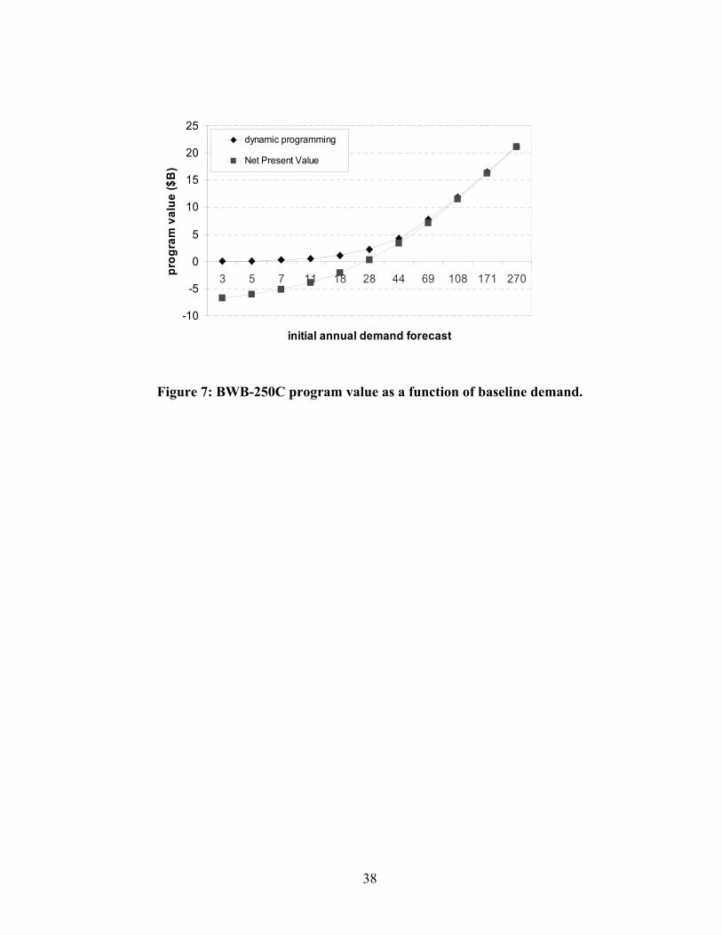
Figure 7 is a plot showing program value for the single aircraft case as a function of the initial

annual demand forecast. This demand level is a strong function of the characteristics of the

aircraft—specifically, the range and seat count—but is also dependent upon the current condition

of the market, and the resulting expectations and needs of the airlines. The plot thus considers

the sensitivity of the program’s success to the current condition of the market. Demand is

expressed as the number of aircraft per year that are demanded in year 1 of the analysis. This

initial quantity is the starting point for the evolution of demand according to a stochastic process

over the time horizon of the problem.

Figure 7 shows two plots of value on the same set of axes: “dynamic programming” and “Net

Present Value”. The former shows the output of the algorithm as it finds the value of the

program using DP to account for managerial flexibility. The latter is the NPV case described

above, where flexibility is removed from the program. As the initial demand forecast increases,

expected program value increases. If the forecast is very small, the value of the program with no

flexibility is negative—that is, the aircraft is developed, the non-recurring cost is incurred, but

few if any units are sold. However, the value with flexibility for low demand indices is zero—if

no sales are expected, no investment is made in developing the aircraft.

25

As the demand index increases, the no-flexibility program value quickly approaches value

with flexibility. However, for small or marginal demand index numbers, there is a significant

difference between the two valuations—one that may mean the difference between keeping a

program and scrapping it. At the baseline initial demand of 28 aircraft per year, the value with

flexibility, $2.26B, is almost seven times the value without flexibility, $325M.

Aircraft Family Valuation

Using the DP method, the three aircraft designs listed in Table 2 are evaluated in several

different combinations to find program value. First, each of the designs is evaluated on an

individual basis, as though it is the only design option available to the firm. Then, the BWB-450

and BWB-250C are evaluated simultaneously, to investigate any synergies that may exist as a

result of commonality. Finally, the BWB-450 and BWB-250P are also evaluated simultaneously.

The key input parameters used for all test cases are listed in Table 3.

Table 3. Key input parameters for all test cases.

Number of periods 30

Timestep per period 1 year

Risk-free rate, rf 5.5%

Annual aircraft price inflation 1.2%

Annual aircraft demand volatility 19.6%

The intermediate results of the test runs described above are summarized in Table 4. These

represent the primary outputs of the models described in this paper: cost characteristics and

demand characteristics based upon a particular airframe and its performance. It can be seen that

there is greater annual demand for the smaller capacity aircraft than for the larger BWB-450.

26

Note that quantity demanded is modeled as independent of operating characteristics—rather, the

quantity estimator considers only the size class of the aircraft. However, the price estimator

distinguishes between all three vehicles. The baseline price is expectedly high for the BWB-450,

as it is a much larger aircraft. However, while the two smaller aircraft have identical seat counts,

the BWB-250P is significantly higher priced. This effect is due to its lighter weight, which

results in significantly reduced fuel burn, and therefore a lower operating cost.

Table 4. Intermediate results: cost and demand characteristics for BWB family.

Design Baseline quantity

demanded (units/yr)

Long-run marginal

cost ($M) Baseline price ($M)

BWB-450 16.7 139.0 195.0

BWB-250C 27.6 93.8 116.1

BWB-250P 27.6 84.9 142.2

Predictably, LRMC scales with the vehicles’ weight. For this example, the LRMC is defined

as the marginal cost of unit 100, produced without any commonality effects. Thus, because the

point-designed BWB-250P is lighter than the derivative BWB-250C, its long-run cost of

production is smaller. However, commonality should result in a reduced development cost and a

reduced learning effort for the BWB-250C. That is, the marginal cost should reach LRMC faster.

Table 5 shows the final results of this example: the program values resulting from the several

different combinations of designs evaluated. The first result to consider is the extremely high

program value found for the BWB-250P. While it is probably too high to be realistic, it

highlights the key design issues in this example: a considerable sacrifice was made in the 250-

passenger class aircraft design to accommodate commonality. A modest increase in empty

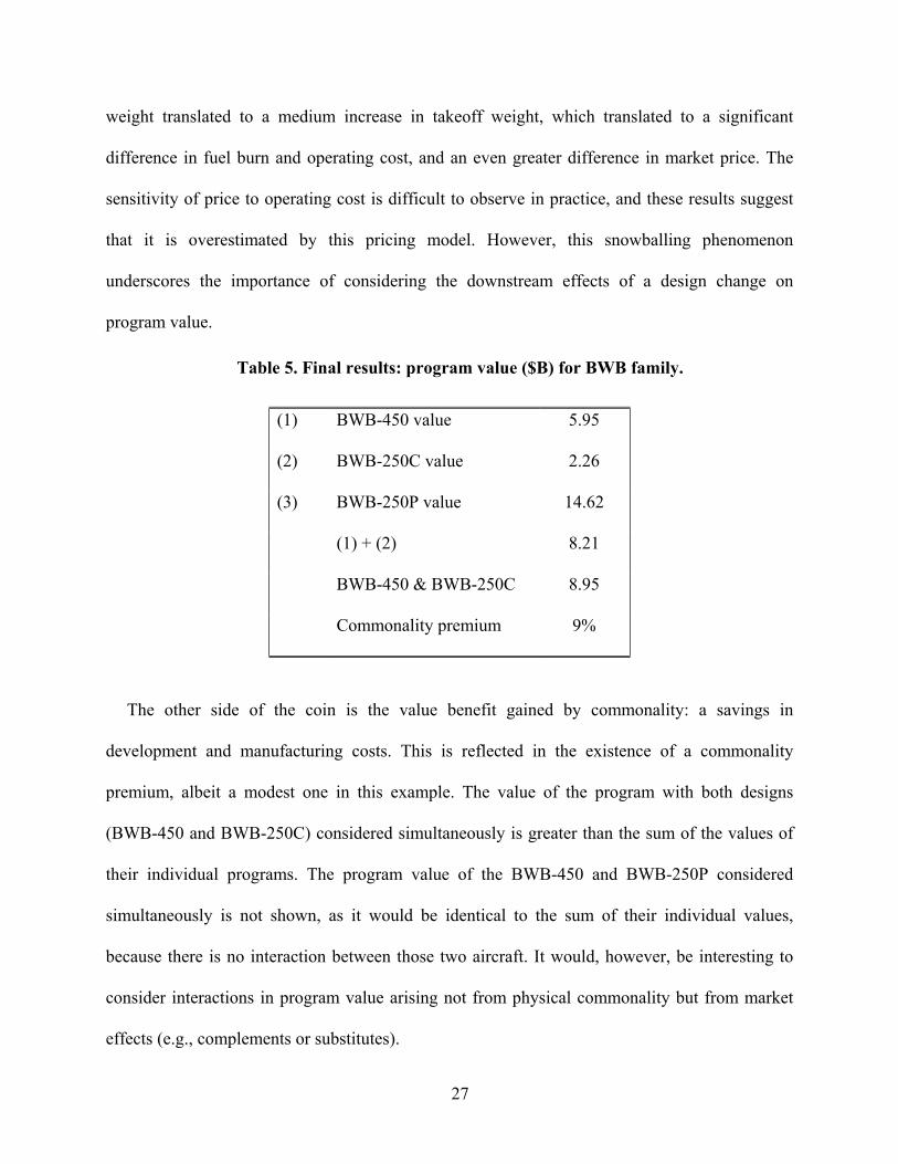
27

weight translated to a medium increase in takeoff weight, which translated to a significant

difference in fuel burn and operating cost, and an even greater difference in market price. The

sensitivity of price to operating cost is difficult to observe in practice, and these results suggest

that it is overestimated by this pricing model. However, this snowballing phenomenon

underscores the importance of considering the downstream effects of a design change on

program value.

Table 5. Final results: program value ($B) for BWB family.

(1) BWB-450 value 5.95

(2) BWB-250C value 2.26

(3) BWB-250P value 14.62

(1) + (2) 8.21

BWB-450 & BWB-250C 8.95

Commonality premium 9%

The other side of the coin is the value benefit gained by commonality: a savings in

development and manufacturing costs. This is reflected in the existence of a commonality

premium, albeit a modest one in this example. The value of the program with both designs

(BWB-450 and BWB-250C) considered simultaneously is greater than the sum of the values of

their individual programs. The program value of the BWB-450 and BWB-250P considered

simultaneously is not shown, as it would be identical to the sum of their individual values,

because there is no interaction between those two aircraft. It would, however, be interesting to

consider interactions in program value arising not from physical commonality but from market

effects (e.g., complements or substitutes).

28

Within the framework of flexibility and decision-making used by the dynamic programming

algorithm, the choice to use commonality may be framed using Real Options. When the firm

develops the BWB-450, it acquires an option to develop the BWB-250C for a reduced cost and

at a time of its choosing. The penalty paid—i.e., the price of the option—is the present value of

additional profits the firm would receive had it instead developed the BWB-250P as a point

design to maximize its performance. From a program flexibility standpoint, the firm still has an

option to develop a second aircraft even if there is no commonality—in such a case, the exercise

price of the option is simply higher by the amount of cost savings from commonality.

The conclusion of this example, therefore, is not that commonality isn’t justifiable. Rather, for

commonality to be justifiable, the benefits must outweigh the costs. The benefits include the

development and manufacturing cost savings gained if the derivative aircraft is in fact built. The

costs include any additional design or manufacturing costs as a result of commonality, but most

importantly, any resulting performance penalty on the aircraft. This performance penalty must be

translated into an opportunity cost: the revenues foregone by not selling a higher-performance

aircraft. The set of aircraft designs used in this example, with the baseline parameters specified,

did not indicate a higher program value for commonality, because the opportunity cost of lost

revenues was very high.

CONCLUSIONS

This paper presents an aircraft program valuation tool, which combines performance, cost and

revenue models, and a DP algorithm to measure the value of a set of aircraft designs to a firm.

The value measurement is not based upon any technical characteristics per se, or any static

forecast of cost and revenue, but on an analysis of an uncertain future, assuming that value-

maximizing decisions are made by management as time goes on and uncertainty is resolved. The

29

approach, which parallels Real Options analysis, provides additional insight over traditional

valuation techniques by its attempt to quantify the value created by flexibility. Flexibility is

modeled and addressed by the DP “operating modes” formulation, which is an explicit method of

formalizing and discretizing the decision-making process that is continuously ongoing for any

project at any firm. Two of the method’s distinguishing features are the combination of

economic analysis with engineering analysis and explicit consideration of management’s ability

to make and defer decisions in “real time” in response to unfolding market conditions.

One important question that has not been addressed here is the impact on the results of

uncertainty in the cost and performance estimates. While it is possible to think of adding cost or

one performance metric as an additional stochastic variable, the computational demands of the

DP algorithm make this approach very challenging, if not impossible. One could conceive of a

two-step process, where the DP approach is used to first determine a set of decision rules and

then a more traditional MCS is subsequently applied to determine the effect of additional

uncertainty on the valuation results. These extensions are the subject of ongoing research.

ACKNOWLEDGMENTS

The authors gratefully acknowledge the help of the BWB team in developing many of the

models and concepts presented here. In particular, we would like to thank Bob Liebeck, John

Allen, George Busby, Richi Gilmore, Josh Nelson and Sean Wakayama. In addition, we thank

Dave Anderson, Earll Murman and Stewart Myers for their input and support and D. Bertsimas,

MIT Sloan School of Management, for suggesting the view of dynamic programming presented

here. This work was supported by the Lean Aerospace Initiative and the National Science

Foundation.

REFERENCES

30

1 Zang, T. A., Green, L. L, “Multidisciplinary Design Optimization Techniques: Implications

and Opportunities for Fluid Dynamics Research,” AIAA Paper 99-3798, presented at 30th AIAA

Fluid Dynamics Conference, Norfolk, VA, 28 June – 1 July, 1999.

2 Kroo, I. “MDO Applications in Preliminary Design: Status and Directions,” AIAA Paper 97-

1408, presented at 38th AIAA Structures, Structural Dynamics, and Materials Conference,

Kissimmee, FL, Apr. 7-10, 1997.

3 Kirby, M.R. and Mavris, D.N., “Forecasting Technology Uncertainty in Preliminary Aircraft

Design,” SAE Paper 1999-01-5631, presented at the 4th World Aviation Congress and

Exposition, San Francisco, CA, Oct. 19-21, 1999.

4 Mavris, D.M. et al., “A Stochastic Approach to Multi-disciplinary Aircraft Analysis and

Design,” AIAA Paper 98-0912, presented at the 36th Aerospace Sciences Meeting and Exhibit,

Reno, NV, Jan. 12-15, 1998.

5 Mavris, D.M. and Birney, M., “Formulation of a Stochastic, Physics-Based Strategic Business

Decision Making Environment,” AIAA Paper 2002-5850, presented at the AIAA ATIO Forum,

Los Angeles, CA, Oct. 1-3, 2002.

6 Younghans, J.L. et al., “An integrated probabilistic approach to advanced commercial engine

cycle definition”, ISABE Paper 99-7194, 14th International Symposium on Air Breathing

Engines, Florence, Italy, Sept. 1999.

7 Dixit, A. K. and Pindyck, R. S., Investment Under Uncertainty, Princeton University Press,

Princeton, NJ, 1994.

8 Trigeorgis, L. Real Options: Managerial Flexibility and Strategy in Resource Allocation, MIT

Press, Cambridge, MA, 2000.

9 Liebeck, R. H., Page, M. A., Rawdon, B. K., “Blended-Wing-Body Subsonic Commercial

Transport,” AIAA Paper 98-0438, Jan. 1998.

10 Wakayama, S., “Blended-Wing-Body Optimization Problem Setup,” AIAA Paper 2000-4740,

Sept. 2000.

11 Wakayama, S., Lifting Surface Design Using Multidisciplinary Optimization, Ph.D. Thesis,

Dept. of Aeronautics & Astronautics, Stanford University, Dec. 1994.

12 Mavris, D.M., Nottingham, C.R. and Bandte, O., “The Impact of Supportability on the

Economic Viability of a High Speed Civil Transport,” presented at the 1st Joint International

Conference of the International Society of Parametric Analysts and the Society of Cost

Estimating and Analysis, Toronto, Canada, June 1998.

13 Markish, J., “Valuation Techniques for Commercial Aircraft Program Design,” S.M. Thesis,

Dept. of Aeronautics & Astronautics, Massachusetts Institute of Technology, June 2002.

14 Markish, J. and Willcox, K., “Multidisciplinary Techniques for Commercial Aircraft System

Design”, AIAA Paper 2002-5612, Sept. 2002.

15 Aircraft Value News Aviation Newsletter, http://www.aviationtoday.com/catalog.htm.

16 The Airline Monitor, ESG Aviation Services, Ponte Vedra Beach, FL, May 2001.

17 Boeing Current Market Outlook, 2000, App. B, p. 42.

18 Airbus Global Market Forecast, 2000-2019, App. G, Detailed passenger fleet results, p. 74.

19 The Airline Monitor, ESG Aviation Services, Ponte Vedra Beach, FL, July 2000, Projected

Jet Airplane Deliveries—2000 to 2020, pp. 10-11.

20 Kulatilaka, N., “Valuing the Flexibility of Flexible Manufacturing Systems,” IEEE

Transactions on Engineering Management, Vol. 35, No. 4, pp. 250-257, Nov. 1998.

31

technical trades • configuration

• performance

program trades • product mix

• timing • cost

• pricing

Valuation Algorithm

program value

Per for mance Es ti mator / Configuration Opti mizer

Manufac turi ng Cos t/ Development C ost Model

Program Structure • Decision tree

• Prici ng str ateg y

Demand Model

Program Val ue

Produc t C onfigur ati on Database

Aircraft T ypes: a, b, c , …

Figure 1: Value-based design process.

32

0 10 20 30 40 50 60 70 80

0 10 20 30 40 50 60 70 80 Actual price ($M)

Estim

ated

pric

e ($

M)

y=x Airbus Boeing

0 20 40 60 80

100 120 140 160

0 20 40 60 80 100 120 140 160 Actual price ($M)

Estim

ated

pric

e ($

M)

y=x Airbus Boeing

Figure 2: Price model results. Top: narrowbodies; bottom: widebodies.

33

0

500

1000

1500

2000

2500

3000

3500

4000

100 125 150 175+ 200 250 300 350 400 500+

Seat Category

Qua

ntity

Airbus

Airline Monitor

Boeing

Figure 3: 20-year gross demand—forecasted deliveries through 2019.

34

0CANNOT remain in this mode

1Design CAN remain in this mode

2

3

4 7 10

5 8 11 Tooling &Capital Investment

6 9 12

13 14 15 Production

16 Abandonment

LOW MEDIUM HIGHCAPACITY CAPACITY CAPACITY

Figure 4: Operating mode framework for a single aircraft.

35

0

25

50

75

100

125

150

175

200

1 3 5 7 9 11 13 15 17 19 21 23 25 27 29 31

Time (years)

Qua

ntity

dem

ande

d pe

r yea

r

waitdesignbuildlo->medlo->hi

Figure 5: Decision rules for BWB-250C.

36

0123456789

10111213141516

0 2 4 6 8 10 12 14 16 18 20 22 24 26 28 30

time (years)

oper

atin

g m

ode

0

20

40

60

80

100

120

quan

tity

dem

ande

d pe

r yea

r

modedemand

-4,000,000

-3,000,000

-2,000,000

-1,000,000

0

1,000,000

2,000,000

3,000,000

0 2 4 6 8 10 12 14 16 18 20 22 24 26 28 30

time (years)

cash

flow

($K

)

Figure 6: Simulation run for BWB-250C. Top: quantity demanded per year and

resulting choice of operating mode. Bottom: associated cashflows.

37

-10

-5

0

5

10

15

20

25

3 5 7 11 18 28 44 69 108 171 270

initial annual demand forecast

prog

ram

val

ue ($

B)

dynamic programming

Net Present Value

Figure 7: BWB-250C program value as a function of baseline demand.

38