Valuing Air Pollution in Britain - Home | IZA · Valuing Air Pollution in Britain Arnaud Chevalier and Eleftherios Giovanis ... pollution and happiness using panel micro-data in Britain,

1

Valuing Air Pollution in Britain

Arnaud Chevalier and Eleftherios Giovanis

Royal Holloway University, Department of Economics

Abstract

This study explores the relationship between happiness and air pollution in Britain using data from the British Household Panel Survey (BHPS). The effects of air pollution on individuals’ happiness are estimated and their monetary value is calculated. In particular, three air pollutants are examined in this paper; the sulphur dioxide (SO2), the ground-level ozone (O3) and the nitrogen dioxides (NOX). Moreover, two different approaches are followed. The first approach refers to panel fixed and random effects regressions. The second model considers fixed effects with lagged dependent variable. The results show that the SO2 presents the strongest negative effects on well-being happiness followed by O3 and NOX. However, ozone’s and nitrogen oxides’ monetary costs are very low in comparison with sulphur dioxide.The monetary values for sulphur dioxide range between £12-£18, while the respective values for ground level ozone and nitrogen oxides range between £3-£6 and £2 respectively.

JEL: C23, Q51, Q53

Keywords: Air pollution, Environmental valuation, Happiness, Life satisfaction approach, Subjective well-being

2

1. Introduction

Economists have long worried about valuing the environment (see Leontief, 1970

for an early example). The difficulty steams from the absence of markets pricing the

environment/pollution. More specifically, environmental externalities are usually

negative and because of the absence of the markets and market prices the economic

agents have no concept of their actions on the environment. To value the

environment, two popular methods exist: revealed preference and stated preference.

The first method relies on hedonic price analysis or the travel cost approach while the

stated preference approach, based on contingent valuation surveys, directly educidate

the environmental value from question. Both methods have been widely used in

practice (Carson et al. 2003). Both methods have weaknesses. Revealed preference

approaches are based on stringent assumptions concerning the rationality of agents

and the functioning of markets. More specifically, the results yielded following this

approach can be biased, if the housing markets are not in equilibrium, maybe because

individuals are not fully informed.

Moreover, using the hedonic method the results can be underestimations of the

clean air benefits (Bayer et al. 2006). More specifically, decisions in markets for

private goods may not accurately reveal people’s hedonic experience from the

consumption of public goods (Rabin, 1998).

1. The European Carbon market is an exception, European Commission Climate Action, 2005

3

In the stated preference approach, hypothetical scenarios are used, which may

entail unreliable results. In particular, the hypothetical nature of the surveys allow for

strategic behaviour and superficial answers (Kahneman et al., 1999). Overall, the

problem of both approaches is that they only value the environmental goods of which

individuals are aware of.

Instead this paper relies on life satisfaction evaluation (LSE). One advantage of

this method is that it does not rely on asking people how they value environmental

conditions. More specifically, individuals are not asked to value the environmental

good directly, but to evaluate their general life satisfaction. Therefore, the LSE

approach does not require awareness of cause-effects relationships but simply

assumes that pollution leads to change in life satisfaction. These changes can be

driven by observed or unobserved pollution. For example, if unobserved pollution

leads to a health deterioration which triggers a reduction in life satisfaction. LSE is

thus closely related to hedonic pricing but relies on life satisfaction rather than house

price to evaluate how individuals value their environment. As such, it is not subject to

market distortion and can be used even in area with shallow housing markets2

This is closely related to hedonic pricing but relies on life satisfaction rather than

house price to evaluate how individuals value their environment. As such, it is not

subject to market distortion and can be used even in area with shallow housing

markets. Indeed the depth of the housing market may well be correlated with

pollution, leading to selection bias in hedonic pricing analysis.

2. Indeed the depth of the housing market may well be correlated with pollution, leading to selection bias in hedonic pricing analysis

4

Additionally, with life satisfaction approach the individual’s demand can be

captured, while using other approaches the individuals have limited incentive to

disclose their true demand (Luechinger, 2009; Frey et al., 2009; MacKerron and

Mourato, 2009). Furthermore, this approach does not rely on an equilibrium

assumption (Frey et al., 2009). More precisely, LSE does not rely on the ability of the

respondents to account and consider all the relevant consequences of a change in the

provision of a public good. For example, the respondents might not notice that there is

a relationship between environmental conditions and their subjective well-being.

Additionally, the strategic behaviour might be avoided because the relationship

between life satisfaction and the environmental good is made ex post by the

researcher. On the other hand, there is the argument that a respondent exposed to a

negative externality, he or she might strategically report an overly low life

satisfaction. However, this can be a minor problem in LSE for the reason that life

satisfaction data are usually collected for many and various purposes. Therefore, the

same data can be used for a wide array of environmental goods evaluation, leading to

the prevention of strategic behaviour and biases.

The contribution of this study is the exploration of the association between air

pollution and happiness using panel micro-data in Britain, while other studies use

panel macro-level data or cross section micro-level data. Moreover, other studies

examine micro-level panel data taking into consideration the clustering on individual

or household level, while the clustering on location or district is been ignored.

The paper explores the relationship between air pollution and well-being

happiness using data from the British Household Panel Survey. The paper is

organized as follows. Section 2 presents a short literature review. Section 3 describes

the methodological framework. In section 4 the data and the research sample design

5

are provided. In section 5 the results of estimating several versions of a happiness

function, with air pollution included, are reported, as well as, the effects of air

pollution on happiness and their monetary value are presented and discussed. In

section 6 the concluding remarks are presented.

3. Literature Review

Research studies on happiness have identified various personal, demographic and

socio-economic factors of happiness that explain observed happiness patterns. Some

of the most important personal and demographic characteristics which affect

happiness are age, sex, marital status, the size of the household and the education

level. Sandvik et al. 1993 have shown that respondents who are satisfied with their

lives are also rated as satisfied by family members and friends. Blanchflower and

Oswald (2007) found that satisfied individuals are less likely to suffer from

hypertension. Furthermore, life satisfaction predicts future marriage and future marital

break-up (Gardner and Oswald 2006; Stutzer and Frey, 2006). There is the general

belief that data on subjective well-being are valid and can be used for formal analyses

(Di Tella et al., 2003; Pischke, 2011).

Empirical work has demonstrated that economic conditions like income,

unemployment and inflation have a strong impact on people’s subjective well-being

(Clark and Oswald, 1994; Di Tella et al., 2001; Easterlin, 2001). The life satisfaction

6

evaluation (LSE) computes the monetary equivalent of any determinant of satisfaction

by dividing the estimated coefficient for this variable of interest on the estimated

coefficient for income.

More specifically, the estimated coefficients can be interpreted as marginal

utilities of the public goods or the marginal dis-utilities of the public bads. Together

with estimates for the marginal utility of income, the marginal rate of substitution

between income and the public good can be calculated. Thus, reported subjective

well-being can serve as an empirically adequate and valid approximation for

individually experienced welfare. Hence, it is a straightforward strategy for the direct

evaluation of a public goods or bad expressed in utility terms (Clark and Oswald,

1996).

The LSE has been used by Welsh (2002; 2006; 2007) to evaluate environmental

factors. More precisely, Welsch (2002; 2006; 2007), examines average life

satisfaction in relation to average air pollution values across countries and he finds

significant negative associations in each case. Ferreira et al. (2006), using individual-

level data on air pollution and other environmental quality parameters in Ireland, find

negative associations between air pollution and life satisfaction. Rehdanz and

Maddison (2008) find that perceived levels of air pollution are also negatively related

to life satisfaction scores in Germany using information about how strongly the

respondent feels affected by air and noise pollution in their place of residence. One

drawback of this study is that the analysis is based on subjective measures rather than

objective measures.

Welsh notes that LSE does not require the awareness of individuals about the

cause-effect relationship between their own health or happiness and the environmental

conditions. However, the awareness of air pollution may reduce individuals’

7

happiness directly and independent of the possible health effects. Moreover, based on

Bickerstaff and Walker’s (2001) study individuals are generally aware of pollutions

sources, mainly the road traffic, the fluctuations on pollutions emissions, because of

the meteorological and weather conditions, and their effects on health.

One major limitation of these studies is the individual identification at the same

level. Roback (1982, 1988) circumvent at this limitation by assuming that households

with identical wage-earning capacities are at the same welfare level. More over, this

is based on the assumption that households present identical utility functions, as well

as, this approach is based on the assumption of perfect mobility.

Welsh (2002) examined the water pollution in 54 countries during early and mid

of 1990s and he found that marginal-willingness-to-pay (MWTP) is $113 for nitrogen

dioxides (NO2). Similarly, Welsh (2006) using repeated cross-section for 10 European

countries during period 1990-1997 found that MWTP is valued at about $184 per

capita per year in the case of lead. Based on Di Tella and MacCulloch’s study (2007),

the MWTP is valued at $171 for sulphur dioxides (SOX). Luechinger (2009)

examined 13 European countries during period 1979-1994 and the MWTP is $157 for

sulphur dioxide (SO2), while it becomes larger at $324 when instrumental variable

estimates are considered. Similarly, Luechinger (2010) using data from the German

Socio-Economic Panel (GSOEP) for about 450 German counties during period 1985-

2003 finds that MWTP is valued at $200 for sulphur dioxide (SO2). However, using

IV estimates the MWTP becomes $340.

8

4. Methodology

Happiness and life satisfaction can serve as an empirically valid and adequate

approximation of individual welfare, in a way to evaluate directly the public goods.

Additionally, by measuring the marginal disutility of a public bad or air pollution in

that case, the trade-off ratio between income and the air pollution can be calculated.

Therefore, the individual’s reported happiness or life satisfaction levels can be treated

as proxy utility data. More specifically, the life satisfaction approach assumes that

interpersonal comparisons of utility are meaningful (Clark and Oswald, 1996).

tjitjitktjititjtji lWzyeLS ,,,,,,2,10,, ')log( εθµγββββ ++++++++= (1)

The set tje , is the measured air pollution in location j and in time t. )log( ,tiy

denotes the logarithm of personal or household income and z is a vector of all the

other possible household and demographic factors, discussed in the next section. W is

a vector of meteorological variables, as mean temperature and wind speed in location-

city k and in time t3.

3. Both calendar effects and weather affect life satisfaction; see for example Brereton et al. (2007) for the effect of wind speeds and temperature and pollution. Wind and temperature may also have a direct effect on the prevalence of pollution

9

Set iµ denotes the individual-fixed effects, jl is a set of location (local

authority) fixed effects and tθ is a time-specific vector of indicators for the day and

month the interview took place and the survey wave. Finally, tji ,,ε expresses the error

term which we assume to be iid. Standard errors are clustered at the local authority

level.

For a marginal change of e, the marginal willingness-to-pay (MWTP) can be

derived from differentiating (1) and setting dLS=0. This is the income drop that

would lead to the same reduction in life satisfaction than an increase in pollution.

Thus, relation (1) becomes:

LS

f

e

f

de

dLSMWTP

∂

∂

∂

∂=−= / (2)

Such a model is identified from changes in the pollution level within individuals

(i.e. between interviews) rather than between individuals. To capture unobservable

characteristics of the neighbourhood that may be correlated with pollution and life

satisfaction, the model is estimated for a population of non-movers since the decision

to move may well be correlated with pollution level. The identification is thus

crucially dependent on variation in the pollution level between interviews. We argue

that this is possibly exogenous and driven by differences in the time of the year that

the interviews take place, as well as variation in the level of pollution between years

due to variations in economic activity, weather conditions, and general reduction of

pollution over time. Evidence of these exogenous changes is provided in the data

section. Of course, time of interview and weather may have a direct effect on self-

reported life satisfaction, it is thus important to directly control for these variables.

10

In its current form the model can be estimated by ordered probit or logit.

Therefore, the dependent ordinal variable is converted in such a form where ordinary

least squares can be applied. This procedure was introduced by van Praag and Ferrer-

i-Carbonell (2004). More specifically, when the dependent variable is categorical, the

ordinary least squares (OLS) method can no longer produce the best linear unbiased

estimator (BLUE); that is, the OLS is biased and inefficient (van Praag and Ferrer-i-

Carbonell, 2004).

More precisely, the categorical dependent variable is rescaled by deriving Z-

values of the standard normal distribution that correspond to cumulative frequencies

of the original categories. The calculation of the dependent ordinal variable can be

stated as:

)]()(/[)]()([)|( 122121,, µµµφµφµµ Φ−Φ−=<<= ZZELS tji (3)

, where Z is a standard normal random variable, φ is the standard normal probability

density function, and Φ is the standard normal cumulative density function.

Finally, the regressions are estimated for each air pollutant separately. The reason

is that the data are available in different dates for each pollutant.

Concerning the samples used, the movers might tend to be more individualistic

and less loyal to where they live. However, the total sample is considered to account

for all respondents. On the other hand by restricting the sample to non-movers some

bias associated with unobserved characteristics might be removed. A location fixed

effect may derive, for example living to rural or urban areas, or living close to natural

attractions as rivers. Furthermore, recent research has shown that the collective self is

more central to identity and well-being among non-movers individuals than among

11

movers (Oishi et al., 2007). Therefore, the relation between national happiness or life

satisfaction and air pollution might be stronger among non-movers than movers.

4. Data

We use the British Household Panel Survey (BHPS) an annual survey of each

adult member of a nationally representative sample of more than 5,000 households

which started in 1991 and stopped in 2009. Individuals moving out or into the original

household are also followed (Taylor et al., 2010). The data period used in the current

study covers the waves 1-18, i.e. years 1991-2009.

Based on the happiness literature the demographic and household variables used

in this study are income, gender, age, age squared, family size or household size, job

status, house tenure, marital status, the education level and qualification, health status

and local authority districts. Additionally, the regressions control for the day of the

week, month of the year and the wave of the survey. Moreover, the minimum,

maximum and average temperature, precipitation and wind speed are considered as

additional variables.

Regarding the dependent variable, the general happiness is taken. More

specifically there are two questions in the survey: one about their overall life

satisfaction and one about their general happiness at the moment the question is

asked. The second question is used to identify the effect of contemporaneous local

pollution. General happiness is an ordinal variable measured on a 4-point scale

representing respectively “much less happy”, “less happy”, “same as usual” and

12

“happier than usual”. The specific question is “what is your level of general

happiness”.

We focus on three air pollutant: ground-level ozone (O3), sulphur dioxide (SO2),

and nitrogen dioxides (NOx) can be found at the website of the Department for

Environment Food and Rural Affairs (DEFRA, http://uk-air.defra.gov.uk). The air

pollutants are based on daily frequency and measured in µg/m3. There are 96

monitoring stations for SO2, 109 for O3 and 156 for NOX. The respondents’ authority

district located within 10 miles radius is considered in regression analysis.

Sulphur dioxide (SO2) is a colourless gas, released from burning fossil fuels like

coal and oil. It is one of the main chemicals that cause acid rain. Usually, power

stations and oil refineries are the main sources of sulphur dioxide. Additionally, SO2

has long been recognised as a pollutant because of its role in forming winter-time

smogs. High concentrations of SO2 can result in breathing problems with asthmatic

children and adults who are active outdoors. Furthermore, short-term exposure has

been linked to wheezing, chest tightness and shortness of breath, while long-term

exposure is associated with respiratory illness and cardiovascular diseases (Harrison,

2001). The daily limit value for the protection of human health is 125 µg/m3. More

specifically, sulphur dioxide emission should not be exceeded 125 µg/m3 more than 3

times a calendar year.

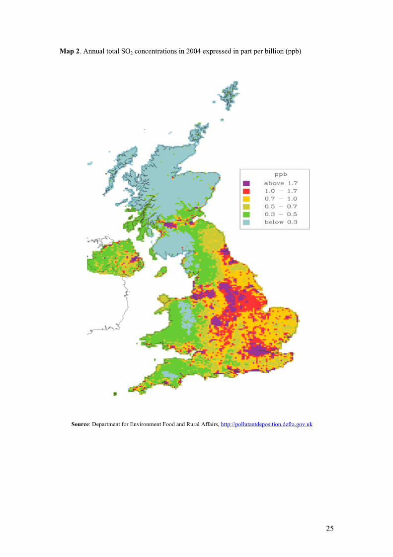
In maps 1-4 the sulphur dioxide total annual concentrations during 1987, 2004,

2006 and 2009 respectively are presented. It becomes clear that the air pollution has

been significantly decreased. The reason is that since the 1960s, the burning of

cleaner fuels, especially natural gas, the decline in heavy industry and the location of

power stations with high stacks outside cities has led to an over 90% decrease in

national average SO2 levels.

13

Ozone (O3) is a gas composed of three oxygen atoms. O3 is a colourless, odourless

gas at ambient concentrations and is the primary constituent and component of smog.

Because smog can be seen, O3 is a pollutant which can be observed by the individuals

too. Furthermore, O3 is known as summer-time air pollutant, because of the peak and

highest values recorded during the high average temperatures. Thus, hot weather

cause ground-level ozone to form in harmful concentrations in the air. Additionally,

motor vehicle exhaust and industrial emissions, gasoline vapours, and chemical

solvents as well as natural sources emit NOx and Volatile Organic Compounds

(VOC) that help form ozone. The effects of ground-level ozone on health include

chest pain, coughing, throat irritation, and congestion, while it can worsen bronchitis,

emphysema, and asthma, as it can reduce lung function and inflame the linings of the

lungs (Harrison, 2001). The UK objective for protection of human health for O3 is 100

µg/m3 with no more than 10 exceedences per year. The annual ground –level ozone

levels are reported in map 5 during the years 1995, 2003 and 2005.

Nitrogen oxides (NOx) are formed in the atmosphere mainly from the breakdown

of nitrogen gas (NO2). Nitrogen oxides are produced in combustion processes, partly

from nitrogen compounds in the fuel, but mostly by direct combination of

atmospheric oxygen and nitrogen. More specifically, NO2 is the component of

greatest interest and the indicator for the larger group of nitrogen oxides and forms

quickly from emissions from cars, trucks and buses, power plants, and off-road

equipment. The effects on health are the same as ozone’s (Harrison, 2001). The

threshold for human protection health is 40 µg/m3.

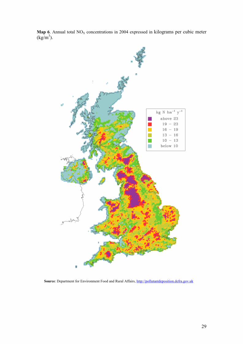
Additionally, the reduction of air pollution is UK was a result of the Large

Combustion Plants Directive 2001/80/EC (LCPD). The Directive’s target is to reduce

the effect of air pollutants throughout Europe. The LPCD came into effect in the UK

14

through the Large Combustion Plants (England & Wales) Regulations 2002, the Large

Combustion Plants (Scotland) 2002 and the Large Combustion Plants Regulations

(Northern Ireland) 2003. The annual nitrogen oxides concentrations during 2004,

2006 and 2009 are presented respectively in the maps 6-8.

In order to minimise measurement error, we take the average air pollution for the

last 30 days4; this also has the advantage of increasing the data coverage since

pollution data is not always available for a given day.

Weather data are taken as additional controls into the estimations. The weather

and meteorological data come directly from MetOffice (www.metoffice.gov.uk) and

National Climatic Data Centre (http://www.ncdc.noaa.gov). More specifically, the

data used is the average, minimum and maximum temperature, precipitation and the

wind speed per city. Moreover weather data are averaged using the same interval as

air pollutants. Temperature is important for ground-level ozone, while the wind speed

can be important for all air pollutants examined (Jacob and Winner, 2009).

Moreover, it should be noticed that the sample of non-movers is 84.00 per cent of

the total sample, while the sample of the movers within GB is 8.50 per cent. The

remaining percentage refers to movers from abroad to GB, to movers where the

location is unknown, to died, to individuals with unknown mover status and to new

entrants in the current wave.

The summary statistics are reported in tables 1 and 2. In table 3 the individual

fixed effects logistic regressions are reported. More precisely, the dependent variable

takes value 1 if the respondent is non-mover and 0 if is a mover across Great Britain.

4.As a robustness check we also conduct the analysis using a 7 days average

15

Furthermore, the monthly air pollution average levels with one lag are included

into the model, in order to examine the possible effects of air pollutants to

individual’s or household’s decision about moving to different place. The results in

table 3 show that the lagged air pollution levels do not affect individual’s choice about

moving in to a different place. Additionally, the weekly air pollution concentration

averages, as well as, the daily pollution levels have been examined leading to the

same conclusions.

The correlation coefficients between the air pollutants are reported in table 4. It

can be observed that the association between NOX and SO2 is positive, while the

relationship between NOX and O3, as well as, SO2 and O3 is positive and significant.

In table 5 the individual fixed effects estimates of air pollution variation during the

month where the interview took place are reported. It is clear that the air pollutants are

varied. More specifically, sulphur dioxide presents significant and positive levels

during March-May, while significant and negative emissions are reported during

August-December. On the other hand, ground-level ozone presents positive and

higher emissions during August, because of the higher temperature levels. Finally,

nitrogen oxides present negative levels, with the exception of February, November

and December, where significant positive emissions are presented.

16

5. Empirical Results and Discussions

5.1 Regression results

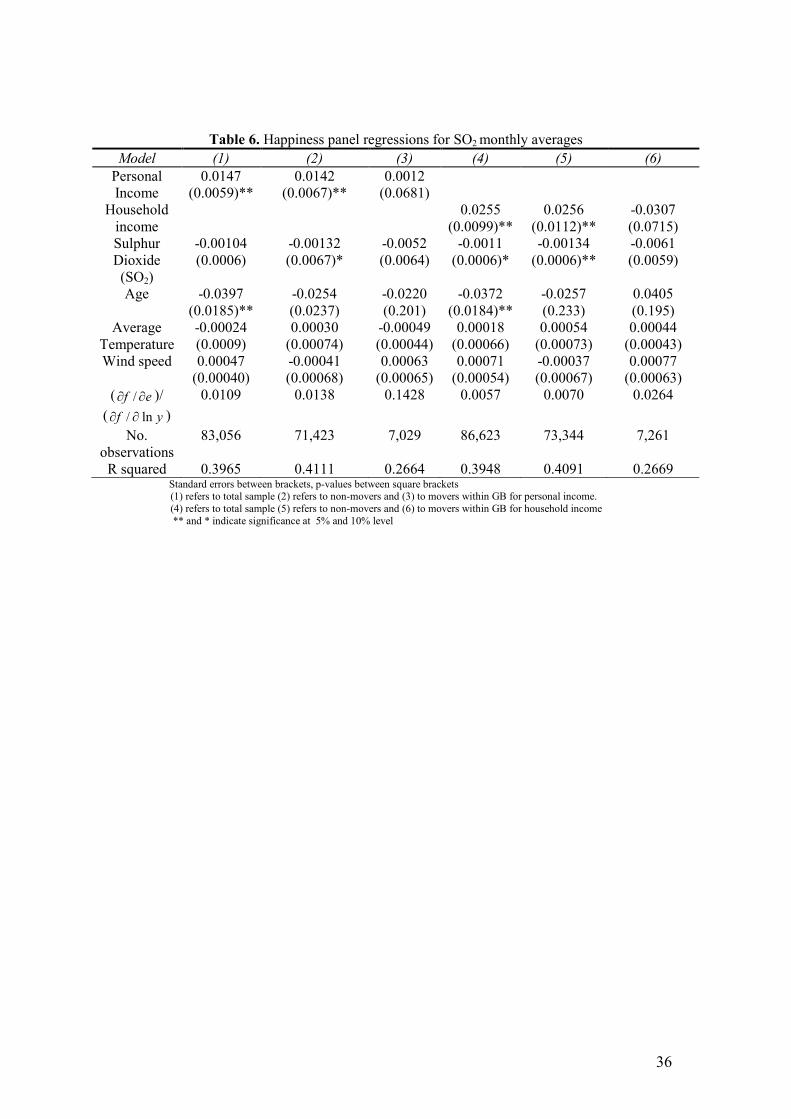
In table 6 the panel regressions for sulphur dioxide monthly averages are

reported5. It can be observed that both personal and household income have a positive

and significant effect on happiness for total sample and the non-movers.

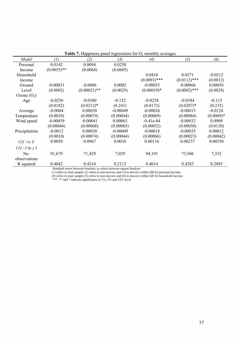
Regarding ground-level ozone monthly averages and the results of table 7 there is

a significant negative association between the specific air pollutant and happiness

only in the case of household income. Similarly, the sign of the household income is

positive and significant. On the other hand, concerning the personal income, ground-

level ozone has a significant and negative effect, only when the non-movers sample is

taken into consideration, while this effect becomes insignificant in the case of the total

sample. Moreover, the personal income is significant and positive only when the

estimations are based on the total sample. Additionally, both personal and household

incomes are insignificant, when the sample of the movers within GB is considered.

Furthermore, the sign of the household income and ozone present the wrong sign.

Finally, in table 8 the estimations for nitrogen oxides monthly averages are

reported. Overall, the estimated coefficients are insignificant, except from the

household income and considering the total sample.

Additionally, the sign of the age, as well as, for gender, concerning random effects

is consistent with other studies’ findings (Rehdanz, and Maddison, 2008; MacKerron

and Mourato, 2009).

5.Based on Hausman test fixed effects are preferred to random effects.

17

It should be noticed that the estimations based on movers sample and household

income show a negative, but insignificant association, between happiness and income.

Furthermore, the household income presents the expected positive sign using random

effects, but it is significant only in the case of ground-level ozone. Additionally, other

specifications of the air pollutants have been examined, as quadratic and cubic,

instead of linear terms, but the coefficients are found to be insignificant. Finally, in

tables 9-11 the regression results for the weekly air pollution average levels are

reported. In this case, the air pollutants present significant and similar effects to those

found when the monthly averages are taken into consideration. In addition, tables 12-

14 present the regression estimates of daily air pollution levels. The only significant

effects are reported in the case of sulphur dioxide, while the effects of ground-level

ozone and nitrogen oxides become insignificant. Nevertheless, ozone’s effects are

again very close with the estimates reported in table 7.

5.2 Marginal willingness-to-pay and price effects

We now compute the marginal willingness-to-pay (MWTP) for our base model. of

sulphur dioxide for the total sample and the non-movers. The individuals are willing

to pay a monthly average of £12 and £15 respectively for a reduction in sulphur

dioxide.

5.Based on Hausman test, random effects are chosen.

18

Similarly, marginal willingness-to-pay (MWTP) of sulphur dioxide for the total

sample and the non-movers, regarding the household income, is 0.0057 and 0.0070

pounds. Thus, the respective average values for household income are £14 and £18.

Regarding, household income and ground-level ozone the MWTP for the total

sample is £3 per month and the maximum monthly value is £100. As for the non-

movers the MWTP is increased to a monthly average of £6 and up to a maximum

value of £173 per month. Moreover, regarding the household income the MWTP is

0.00116 and 0.00237 for the total sample and the non-movers respectively. Similarly,

for nitrogen oxides the MWTP is 0.00173 and 0.00073 for personal and household

income respectively and the total sample. Moreover, the MWTP is significant lower

to those of ozone and sulphur dioxide. More specifically, it is £2 in average per month

and the maximum monthly value is £63, while the estimates concerning the personal

income are insignificant.

5.3 General Discussions

Overall, the results show that sulphur dioxide presents the strongest negative

effects on happiness followed by ground-level ozone and nitrogen dioxides. These

findings are as expected for the following reasons. Firstly, SO2 emissions in United

Kingdom are dominated by combustion of fuels containing sulphur, such as coal and

heavy oils by power stations and refineries. Furthermore, SO2 is classified as a

significant air pollutant because of its role in forming winter-time smogs. This may be

an artefact of the sampling strategy with no interviews taking place in June and July.

At this point it should be noticed that the highest and peak values of O3 are reported

during those months because O3 is depended in a major degree on temperature, as

19

well as it is know as summer-time air pollutant. Therefore, it is very possible that the

estimations for O3 might be underestimated. Furthermore, even if BHPS takes place

during August, it should be mentioned that the respondents interviewed during this

month are very few. Even if the monthly averages of the air pollutants are taken, the

interviews take place during the last days of August. Concluding, both air pollutants,

SO2 and O3 are responsible in forming winter-time and summer-time smogs

respectively, thus the specific air pollutants can be observed by the individuals.

Finally, in table 15 the MWTP for a drop of a standard deviation is reported. More

specifically, regarding the personal income the individuals are willing to pay £92 and

£108, based on total sample and non-movers sample respectively, for a drop of a

standard deviation in sulphur dioxide. This value is increased at £99 and £120 when

the household income is taken into consideration. On the other hand, concerning

ground level ozone, the values are significant only in the case of household income. In

particular the values are £57 and £115 for total sample and non-movers respectively.

Finally, in the case of nitrogen oxides, only value of the total sample considering the

household income is significant and it is £122.

6. Conclusion

This study has used a set of panel micro-data on self-reported well-being

happiness from the British Household Survey. The results showed that the MWTP for

sulphur dioxide ranges between £12-15 and £14-18 per month for personal and

household income respectively, while the respective monthly maximum values range

between £785-980 and £494-510. The MWTP for ground-level ozone and nitrogen

20

oxides is significant lower ranging between £3-6 and £2 per month respectively. The

respective maximum values are £173 and £63. As it was discussed the estimates for

ground-level ozone might be underestimated. The contribution of this paper is that the

life satisfaction approach and air pollution is examined in micro-level data using panel

surveys. Moreover, the results show that the life satisfaction approach contains very

useful information on individuals’ preferences and at the same time expands the

economic tools in the area of non-market evaluation.

Life satisfaction approach has been used to assess how willingness to pay varies

over time and by region, age, income, education and level of pollution among others.

Additionally, one very strong and useful point of the life satisfaction approach is that

the estimated coefficients can be used to calculate the marginal rate of substitution

between income and air quality directly, and thus it does not suffer from the

contingent valuation problem of large gaps between stated willingness to pay and

willingness to accept. Moreover, the life satisfaction approach can be very helpful in

environmental and economic policy planning and decisions.

21

References

Bayer, P.N., Keohane, O., Timmins, C. (2006). Migration and Hedonic Valuation: The Case of Air Quality, NBER Working Paper No.12106, Cambridge, MA: National Bureau of Economics

Bickerstaff, K., Walker, G. (2001). Public understandings of air pollution: the ‘localisation’ of environmental risk, Global Environmental Change, 11, 133–145.

Blanchflower D.G, Oswald, A.J. (2007). Hypertension and Happiness across Nations, Journal of Health Economics, 27, 218-233

Brereton, F., Clinch, J. P., Ferreira, S. (2008). Happiness, geography and the environment, Ecological Economics, 65 (2), 386-396

Carson, RT, Mitchell, RC, Hanemann, WM, Kopp RJ, Presser S, et al. (2003). Contingent Valuation and Lost Passive Use: Damages from the Exxon Valdez Oil Spill, Environmental and Resource Economics, 25, 257–286. Clark, A.E., Oswald, A.J. (1994). Unhappiness and Unemployment, The Economic

Journal, 104, 648-659.

Clark, A.E., Oswald, A.J. (1996). Satisfaction and comparison income, Journal of

Public Economics, 61, 359-381 Di Tella, R., MacCulloch, R., Oswald, A. (2001). Preferences over Inflation and Unemployment: Evidence from Surveys of Happiness, American Economic Review, 91, 335-341.

Di Tella, R., MacCulloch, R.J., Oswald, A.J., (2003). The Macroeconomics of Happiness, The Review of Economics and Statistics, 85, 809-827. Di Tella, R., MacCulloch, R.J. (2007). Gross National Happiness as an Answer to the Easterlin Paradox?, Journal of Development Economics, 86, 22-42.

Easterlin, R.A. (2001). Income and Happiness: Towards a Unified Theory, The

Economic Journal, 111, 465-484. European Commission Climate Action, (2005), Emissions Trading System Ferreira, S., Moro, M., Clinch, J. P. (2006). Valuing the environment using the life-satisfaction approach, Planning and Environmental Policy Research Series Working Paper No. 06/03, School of Geography, University College Dublin

Frey, B.S., Luechinger, S. and Stutzer, A. (2009). The Life Satisfaction Approach to Environmental Valuation, IZA Discussion Paper Series No. 4478 Gardner, J., Oswald, AJ. (2006). ‘Do Divorcing Couples Become Happier by Breaking Up?’, Journal of the Royal Statistical Society Series A, 169, 319-336

22

Harrison, R. M. (2001). Pollution: Causes, Effects and Control, Fourth Edition, The Royal Society of Chemistry, UK Jacob, D.J., Winner, D.A. (2009). Effect of climate change on air quality, Atmospheric Environment,.43 (1), 51–63

Kahneman D, Knetsch J.L. (1992). Valuing Public Goods: The Purchase of Moral Satisfaction, Journal of Environmental Economics and Management, 22, 57-70

Leontief, V. (1970). Environmental Repercussions and the Economic Structure: An Input-Output Approach, Review of Economics and Statistics, 52, 262–271.

Luechinger, S. (2009). Valuing Air Quality Using the Life Satisfaction Approach, The

Economic Journal, 119 (536), 482-515 Luechinger, S. (2010). Life Satisfaction and Transboundary Air Pollution. Economics Letters, 107(1), 4-6

MacKerron, G., Mourato, S. (2009). Life satisfaction and air quality in London, Ecological Economics, 68(5), 1441-1453

Oishi, S., Lun, J., Sherman, G.D. (2007). Residential mobility, self-concept, and positive affect in social interactions, Journal of Personality and Social Psychology, 93, 131–141

Pischke, J.S. (2011). Money and Happiness: Evidence from the Industry Wage Structure, Discussion Paper No. 5705, IZA

Rabin, M. (1998). Psychology and Economics, Journal of Economic Literature, 36(1), 11-46 Rehdanz, K., Maddison, D. (2008). Local environmental quality and life-satisfaction in Germany, Ecological Economics, 64, 787–97 Roback, J. (1982). Wages, Rents and the Quality of Life, The Journal of Political

Economy, 90, 1257–1278 Roback, J. (1988). Wages, Rents and Amenities: Differences Among Workers and Regions, Economic Enquiry, 26, 23–41 Sandvik E, Diener E, Seidlitz L. (1993). Subjective Well-Being: The Convergence and Stability of Self-Report and Non-Self-Report Measures, Journal of Personality, 61, 317-342 Stutzer A, Frey, BS. (2006). Does Marriage Make People Happy, or Do Happy People Get Married?, Journal of Socio-Economics, 35(2), 326-347

23

Taylor, M.F., Brice, J., Buck, N., Lane, E. P. (2010). British Household Panel Survey User Manual Volume A: Introduction, technical report and appendices, Colchester: University of Essex

van Praag, B. M. S., Ferrer-i-Carbonell, A. (2004). Happiness quantified: A

satisfaction calculus approach, Oxford: Oxford University Press Welsch, H. (2002). Preferences over prosperity and pollution: Environmental valuation based on happiness surveys, Kyklos, 55 (4), 473–494

Welsch, H. (2006). Environment and happiness: Valuation of air pollution using life satisfaction data, Ecological Economics, 58, 801–813

Welsch, H. (2007). Environmental welfare analysis: A life satisfaction approach, Ecological Economics, 62 (3-4), 544–551

24

Map 1. Annual total SO2 concentrations in 1987 expressed in part per billion (ppb)

Source: RoTAP 2011: Review of Tranboundary Air Pollution: Acidification, Eutrophication, Ground Level Ozone and Heavy Metals in the UK. www.rotap.ceh.ac.uk

25


Source: Department for Environment Food and Rural Affairs, http://pollutantdeposition.defra.gov.uk

26



27



28

Map 5. Annual total O3 concentrations in 2009 expressed in part per billion (ppb)

Source: Air Quality Expert Group (2009), Ozone in the United Kingdom, http://archive.defra.gov.uk/environment/quality/air/airquality/publications/ozone/documents/aqeg-ozone-report.pdf

29

Map 6. Annual total NOX concentrations in 2004 expressed in kilograms per cubic meter (kg/m3).


30



31



32

Table 1. Summary statistics of income and air pollutants

Variables Mean Standard

Deviation

Minimum Maximum

Panel A: Total Sample

Personal income 1,115.378 1,167.831 0.0 72,176.51 Household

income 2,449.341 1,970.468 0.0 86,703.29

Sulphur Dioxide (SO2)

9.076 15.721 0.1 287.63

Ozone (O3) 34.655 18.204 1.57 135.67 Nitrogen

Dioxides (NOX) 93.474 120.078 0.1 1,742

Panel B: Non-Movers


income 2,516.326 1,981.367 0.0 72,927.47


8.823 16.075 0.1 287.63

Ozone (O3) 34.645 18.346 1.57 133 Nitrogen

Dioxides (NOX) 90.839 118.914 0.1 1742

Panel C: Movers within GB

Personal income 1,191.819 1269.678 0.0 72,176.51 Household

income 2,398.644 2070.24 0.0 86,703.29


9.115 14.949 0.1 232

Ozone (O3) 34.360 18.484 0.0 135.67 Nitrogen

Dioxides (NOX) 96.743 120.175 0.2 1,681

* The air pollutants are measured in micrograms per cubic meter (µg/m3)

33

Table 2. Summary statistics of income and air pollutants controlling for individual fixed effects

Variables Mean Standard

Deviation

Minimum Maximum

Panel A: Total Sample


income 2,449.341 1723.534 0.0 86,703.29


9.076 10.594 0.3 293

Ozone (O3) 34.655 11.457 1.57 109 Nitrogen

Dioxides (NOX) 93.474 75.366 0.2 1,369

Panel B: Non-Movers


income 2,516.326 1728.377 0.0 33,490.25


8.823 10.172 0.3 220

Ozone (O3) 34.645 11.470 1.57 98 Nitrogen

Dioxides (NOX) 90.839 71.361 0.2 1,369

Panel C: Movers within GB


income 2,398.644 1,900.061 0.0 86,703.29


9.115 13.358 0.1 232

Ozone (O3) 34.360 16.778 1.0 124 Nitrogen

Dioxides (NOX) 96.743 109.248 0.3 1681

* The air pollutants are measured in micrograms per cubic meter (µg/m3)

34

Table 3. Fixed effects logistic regressions

Mover status Mover status Mover status

Sulphur Dioxide -0.0022 (0.0021)

Ground-Level Ozone -0.695-04 (0.0009)

Nitrogen Oxides -0.905e-04 (0.0002)

No. observations

22,545 26,716 20,253

LR chi-square 1534.42 [0.000]

2111.22 [0.000]

1789.57 [0.000]

Standard errors between brackets, p-values between square brackets

Table 4. Correlation between air pollutants

Sulphur Dioxide Ground-Level Ozone

Ground-Level Ozone -0.0813 (0.000)

Nitrogen Oxides 0.0106 (0.000)

-0.0559 (0.000)

p-values are reported between brackets.

35

Table 5. Fixed effects estimates for air pollution variation.

Sulphur Dioxide Ground-Level Ozone Nitrogen Oxides

February 0.303 (0.513)

1.299 (0.689)*

5.952 (3.232)*

March 2.827 (0.582)***

2.184 (0.942)**

-13.427 (3.649)***

April 6.193 (0.724)***

2.427 (1.209)**

-20.692 (3.871)***

May 7.812 (1.795)***

0.911 (1.519)

-25.395 (3.917)***

August -6.925 (6.522)***

4.223 (0.590)***

-18.478 (47.356)

September -1.760 (0.335)***

-4.466 (0.574)***

-34.429 (2.594)***

October -3.956 (0.316)***

-3.549 (0.519)***

-18.763 (2.518)***

November -4.42 (0.329)***

-2.413 (0.543)***

3.238 (2.552)

December -5.550 (0.428) ***

0.954 (0.647)

20.761 (2.957)***

No. observations 96,549 95,072 82,338

R squared 0.2520 0.4756 0.3553

Standard errors between brackets, p-values between square brackets ***, ** and * indicate significance at 1%, 5% and 10% level

36

Table 6. Happiness panel regressions for SO2 monthly averages

Model (1) (2) (3) (4) (5) (6)

Personal Income

0.0147 (0.0059)**

0.0142 (0.0067)**

0.0012 (0.0681)

Household income

0.0255 (0.0099)**

0.0256 (0.0112)**

-0.0307 (0.0715)


-0.00104 (0.0006)

-0.00132 (0.0067)*

-0.0052 (0.0064)

-0.0011 (0.0006)*

-0.00134 (0.0006)**

-0.0061 (0.0059)

Age -0.0397 (0.0185)**

-0.0254 (0.0237)

-0.0220 (0.201)

-0.0372 (0.0184)**

-0.0257 (0.233)

0.0405 (0.195)

Average Temperature

-0.00024 (0.0009)

0.00030 (0.00074)

-0.00049 (0.00044)

0.00018 (0.00066)

0.00054 (0.00073)

0.00044 (0.00043)

Wind speed 0.00047 (0.00040)

-0.00041 (0.00068)

0.00063 (0.00065)

0.00071 (0.00054)

-0.00037 (0.00067)

0.00077 (0.00063)

( ef ∂∂ / )/

( yf ln/ ∂∂ )

0.0109 0.0138 0.1428 0.0057 0.0070 0.0264

No. observations

83,056 71,423 7,029 86,623 73,344 7,261

R squared 0.3965 0.4111 0.2664 0.3948 0.4091 0.2669 Standard errors between brackets, p-values between square brackets

(1) refers to total sample (2) refers to non-movers and (3) to movers within GB for personal income. (4) refers to total sample (5) refers to non-movers and (6) to movers within GB for household income ** and * indicate significance at 5% and 10% level

37

Table 7. Happiness panel regressions for O3 monthly averages

Model (1) (2) (3) (4) (5) (6)

Personal Income

0.0142 (0.0055)**

0.0094 (0.0064)

0.0258 (0.0605)

Household income

0.0410 (0.0093)***

0.0371 (0.0112)***

-0.0212 (0.0812)

Ground Level

Ozone (O3)

-0.00031 (0.0002)

-0.0006 (0.00021)**

0.0002 (0.0029)

-0.00035 (0.00019)*

-0.00066 (0.0002)***

0.00056 (0.0028)

Age -0.0256 (0.0182)

-0.0380 (0.0212)*

-0.152 (0.241)

-0.0258 (0.0173)

-0.0384 (0.0207)*

-0.115 (0.235)

Average Temperature

-0.0004 (0.0010)

0.00030 (0.00074)

-0.00049 (0.00044)

-0.00026 (0.00069)

-0.00013 (0.00084)

-0.0126 (0.0069)*

Wind speed -0.00039 (0.00044)

-0.00041 (0.00068)

0.00063 (0.00065)

-0.41e-04 (0.00032)

-0.00032 (0.00030)

0.0909 (0.0130)

Precipitation -0.0012 (0.0010)

0.00030 (0.00074)

-0.00049 (0.00044)

-0.00018 (0.00066)

-0.00035 (0.00023)

0.00012 (0.00042)

( ef ∂∂ / )/

( yf ln/ ∂∂ )

0.0050 0.0967 0.0010 0.00116 0.00237 0.00350

No. observations

91,679 71,429 7,029 94,191 73,506 7,332

R squared 0.4042 0.4314 0.2113 0.4014 0.4283 0.2085 Standard errors between brackets, p-values between square brackets (1) refers to total sample (2) refers to non-movers and (3) to movers within GB for personal income. (4) refers to total sample (5) refers to non-movers and (6) to movers within GB for household income ***, ** and * indicate significance at 1%, 5% and 10% level

38

Table 8. Happiness panel regressions for NOX monthly averages

Model (1) (2) (3) (4) (5) (6)

Personal Income

0.0077 (0.0066)

0.0129 (0.0075)*

-0.0804 (0.144)

Household income

0.01823 (0.0103)*

0.01812 (0.0120)

-0.0918 (0.127)

Nitrogen Oxides (NOX)

-0.09e-04

(0.56e-04)

-0.075e-04

(-0.06e-04)

-0.42e-04

(0.6e-04)

-0.0001 (0.000054)*

-0.09e-04

(0.06e-04)

-0.00045

(0.66e-04)

Age -0.0409 (0.0167)**

-0.0379 (0.0188)**

-0.1310 (0.2613)

-0.0409 (0.0167)**

-0.0355 (0.0187)*

-0.151 (0.253)

Temperature -0.59e-04 (0.00091)

0.00062 (0.00104)

0.0012 (0.0134)

0.00018 (0.00088)

0.00084 (0.00101)

0.0018 (0.0128)

Wind speed 0.58e-04 (0.00032)

-0.00024 (0.00037)

0.00017 (0.00075)

0.57e-04 (0.00031)

-0.00026 (0.00037)

0.80e-04 (0.00070)

( ef ∂∂ / )/

( yf ln/ ∂∂ )

0.00173 0.0009 0.00077 0.00073 0.00065 0.00064

No. observations

72,978 61,464 6,032 75,218 63,312 6,190



39

Table 9. Happiness panel regressions for SO2 weekly averages

Model (1) (2) (3) (4) (5) (6)

Personal Income

0.0166 (0.0059)***

0.0145 (0.0067)**

0.0141 (0.0568)

Household income

0.0260 (0.0101)**

0.026 (0.0113)**

-0.0023 (0.0568)


-0.00103 (0.0006)

-0.00134 (0.0066)**

-0.0037 (0.0051)

-0.0011 (0.0006)*

-0.0013 (0.0006)**

-0.0043 (0.0051)

Age -0.0345 (0.0184)*

-0.0200 (0.0239)

0.0032 (0.171)

-0.0367 (0.0181)**

-0.0251 (0.230)

0.0703 (0.168)

Temperature -0.00162 (0.00086)*

-0.0014 (0.00092)

-0.0123 (0.0111)

-0.0012 (0.00084)

-0.00115 (0.00088)

-0.00837 (0.0089)

Wind speed 0.00068 (0.00057)

0.00086 (0.00068)

0.00018 (0.0024)

0.00071 (0.00056)

0.00091 (0.00065)

-0.00097 (0.0022)

( ef ∂∂ / )/

( yf ln/ ∂∂ )

0.0094 0.0137 0.0393 0.0051 0.0071 0.0132

No. observations

79,177 67,270 6,447 81,764 69,391 6,665


(1) refers to total sample (2) refers to non-movers and (3) to movers within GB for personal income. (4) refers to total sample (5) refers to non-movers and (6) to movers within GB for household income ***, ** and * indicate significance at 1%, 5% and 10% level

40

Table 10. Happiness panel regressions for O3 weekly averages

Model (1) (2) (3) (4) (5) (6)

Personal Income

0.0159 (0.0164)**

0.0101 (0.0075)

0.0172 (0.0217)

Household income

0.0407 (0.0112)***

0.0327 (0.0131)***

-0.0423 (0.0930)

Ground-Level

Ozone (O3)

-0.00043 (0.00025)*

-0.00081 (0.00029)***

-0.00094 (0.00036)

-0.00045 (0.00025)*

-0.00083 (0.0003)***

0.00053 (0.0035)

Age -0.0226 (0.0203)

-0.0283 (0.0251)

-0.244 (0.269)

-0.0256 (0.0200)

-0.0331 (0.0252)

-0.205 (0.262)

Temperature -0.00041 (0.00088)

-0.00087 (0.00110)

-0.00036 (0.0226)

-0.00035 (0.00087)

-0.00069 (0.00109)

-0.00042

(0.00758) Wind speed -0.00066

(0.00077) 0.00138

(0.00117) -0.00190

(0.00380) 0.00059

(0.00079) 0.00132

(0.00119) -0.00055

(0.00446)

( ef ∂∂ / )/

( yf ln/ ∂∂ )

0.0041 0.0119 0.0081 0.00147 0.00331 0.00350

No. observations

70,917 54,167 5,222 73,302 59,987 5,878


41

Table 11. Happiness panel regressions for NOX weekly averages

Model (1) (2) (3) (4) (5) (6)

Personal Income

0.0083 (0.0068)

0.0109 (0.0074)*

0.0062 (0.094)

Household income

0.0227 (0.0101)**

0.0153 (0.0119)

-0.0918 (0.127)


-0.25e-0.4

(0.49e-0.5)

1.82e-05

(0.57e-0.5)

-0.00043 (0.00063)

-0.29e-0.4

(0.49e-0.5)

2.15e-05 (0.56e-05)

-0.00045 (0.00066)

Age -0.0443 (0.0173)**

-0.0374 (0.019)**

-0.0487 (0.210)

-0.0406 (0.0175)**

-0.0352 (0.0191)*

-0.0414 (0.202)

Temperature -0.00111 (0.00009)

-0.0007 (0.00106)

-0.00253 (0.0156)

-0.00089 (0.00094)

-0.00062 (0.00106)

-0.65e-0.4

(0.0144) Wind speed -0.00022

(0.00016) 0.00030

(0.00156) 0.00505

(0.00346) -0.00019

(0.00084) 0.00030

(0.00150) 0.00288

(0.00191)

( ef ∂∂ / )/

( yf ln/ ∂∂ )

0.0004 0.0002

0.0009 0.0012 0.0002 0.0004

No. observations

67,812 57,221 5,458 69,915 58,948 5,606



42

Table 12. Happiness panel regressions for daily SO2

Model (1) (2) (3) (4) (5) (6)

Personal Income

0.0164 (0.0098)*

0.0176 (0.0111)

0.0969 (0.179)

Household income

0.0243 (0.0141)*

0.0230 (0.0141)

0.143 (0.273)


-0.0017 (0.0010)*

-0.0015 (0.0011)

-0.0061 (0.0221)

-0.0018 (0.0010)*

-0.0017 (0.0011)

-0.0069 (0.0208)

Age -0.0568 (0.0333)*

-0.0446 (0.0356)

-0.0202 (0.708)

-0.0502 (0.0316)

-0.0403 (0.0336)

-0.0205 (0.687)

Temperature -0.00201 (0.00140)

-0.00120 (0.00156)

-0.0101 (0.0376)

-0.00191 (0.00142)

-0.00141 (0.00159)

-0.00139 (0.0372)

Wind speed 0.00039 (0.00054)

0.00038 (0.00078)

0.00081 (0.00421)

0.00041 (0.00054)

0.00039 (0.00078)

0.00113 (0.00390)

( ef ∂∂ / )/

( yf ln/ ∂∂ )

0.00016 0.0128 0.0094 0.0103 0.0074 0.0063

No. observations

39,922 34,596 2,778 41,339 35,772 2,896


(1) refers to total sample (2) refers to non-movers and (3) to movers within GB for personal income. (4) refers to total sample (5) refers to non-movers and (6) to movers within GB for household income * indicates significance at 10% level

43

Table 13. Happiness panel regressions for daily O3

Model (1) (2) (3) (4) (5) (6)

Personal Income

0.0112 (0.0073)

0.0074 (0.0082)

0.0180 (0.0600)

Household income

0.0413 (0.0121)***

0.0367 (0.0139)***

-0.0067 (0.0873)

Ground-Level

Ozone (O3)

-0.00036 (0.0004)

-0.0005 (0.00051)

-0.0003 (0.0064)

-0.00033 (0.0004)

-0.00051 (0.0005)

-0.0008 (0.0062)

Age -0.0272 (0.0225)

-0.0475 (0.0245)*

-0.152 (0.241)

-0.0265 (0.0213)

-0.0481 (0.0236)**

-0.0540 (0.323)

Temperature -0.00058 (0.00108)

-0.00145 (0.00125)

0.0183 (0.0200)

-0.00081 (0.00107)

-0.00179 (0.00122)

0.0197 (0.0191)

Wind speed 0.00021 (0.00032)

0.00010 (0.00037)

0.0018 (0.0031)

0.00017 (0.00033)

0.00011 (0.00036)

0.00113 (0.00334)

( ef ∂∂ / )/

( yf ln/ ∂∂ )

0.0101 0.0179 0.0035 0.00091 0.0015 0.0014

No. observations

54,251 45,185 4,217 56,150 46,747 4,341


44

Table 14. Happiness panel regressions for daily NOX

Model (1) (2) (3) (4) (5) (6)

Personal Income

0.0099 (0.0065)

0.0115 (0.0076)

0.0029 (0.1040)

Household income

0.0182 (0.0100)*

0.0154 (0.0118)

-0.0269 (0.081)


0.31e-04 (0.51e-04)

0.49e-04 (0.59e-04)

0.00026 (0.00062)

0.24e-04 (0.51e-04)

0.34e-04 (0.59e-04)

0.00033 (0.00061)

Age -0.0377 (0.0191)**

-0.0349 (0.0236)

0.0861 (0.2939)

-0.0335 (0.0181)**

-0.0329 (0.0224)

-0.1204 (0.273)

Temperature -0.00084 (0.00096)

-0.00103 (0.00109)

-0.00114 (0.0124)

-0.00082 (0.00099)

-0.00094 (0.00111)

-0.00073 (0.0027)

Wind speed 0.00062 (0.00038)

0.00029 (0.00046)

-0.00468 (0.0240)

0.00022 (0.00048)

0.00022 (0.00049)

-0.00471 (0.0200)

( ef ∂∂ / )/

( yf ln/ ∂∂ )

0.0005 0.0006 0.0132 0.0002 0.0003 0.0016

No. observations

64,392 54,382 5,121 66,383 56,020 5,256



45

Table 15. MWTP for a drop of one standard deviation

Sulphur Dioxide Ground-level ozone Nitrogen oxides

Personal Income (total sample) £92 * £70 £120

Household income (total sample) £99 * £57 * £122 *

Personal Income (non-movers sample)

£108* £61 £83

Household income (non-movers sample)

£120 * £115* £127

* Indicates significance

Documents

Valuing Air Pollution in Britain - Home | IZA · Valuing Air Pollution in Britain Arnaud Chevalier and Eleftherios Giovanis ... pollution and happiness using panel micro-data in Britain,