Embed Size (px)
Citation preview
February 2018 THE LEADING EDGE 141a1Special Section: Induced seismicity
Variabilities in probabilistic seismic hazard maps for natural and induced seismicity in the central and eastern United States
AbstractProbabilistic seismic hazard analysis (PSHA) characterizes
ground-motion hazard from earthquakes. Typically, the time horizon of a PSHA forecast is long, but in response to induced seismicity related to hydrocarbon development, the USGS devel-oped one-year PSHA models. In this paper, we present a display of the variability in USGS hazard curves due to epistemic uncer-tainty in its informed submodel using a simple bootstrapping approach. We find that variability is highest in low-seismicity areas. On the other hand, areas of high seismic hazard, such as the New Madrid seismic zone or Oklahoma, exhibit relatively lower variability simply because of more available data and a better understanding of the seismicity. Comparing areas of high hazard, New Madrid, which has a history of large naturally occurring earthquakes, has lower forecast variability than Oklahoma, where the hazard is driven mainly by suspected induced earthquakes since 2009. Overall, the mean hazard obtained from bootstrapping is close to the published model, and variability increased in the 2017 one-year model relative to the 2016 model. Comparing the relative variations caused by individual logic-tree branches, we find that the highest hazard variation (as measured by the 95% confidence interval of bootstrapping samples) in the final model is associated with different ground-motion models and maximum magnitudes used in the logic tree, while the variability due to the smoothing distance is minimal. It should be pointed out that this study is not looking at the uncertainty in the hazard in general, but only as it is represented in the USGS one-year models.
IntroductionProbabilistic seismic hazard analysis (PSHA) (Cornell, 1968;
McGuire, 1976) is a probabilistic forecast of where and how often future earthquakes will occur and how strongly the ground will shake as a result. The output of a PSHA model is a seismic hazard curve obtained by integration of all earthquake scenarios affecting a site. Hazard curves express the annual rates at which different ground-shaking levels are likely to be exceeded at particular sites. Hence, in the context of PSHA, “hazard” refers to the rate (fre-quency) or probability of occurrence of ground-shaking levels, not the value of ground motion. Earthquake occurrence is often assumed to be a Poissonian process (assuming earthquakes occur randomly, and waiting time between events are independent) in the PSHA procedure; hence, each point on a PSHA map represents the shaking level expected to be exceeded once in a T year return period with a fixed probability of p for t years of observations:
p = 1 – e(−t/T ). (1)
S. Mostafa Mousavi1, Gregory C. Beroza1, and Susan M. Hoover2
The USGS is responsible for developing PSHA maps and models for the United States (Algermissen and Perkins 1976; Frankel et al., 1996, 2000, 2002; Petersen et al., 1996, 2008, 2012, 2014). These models are meant to improve public safety, and they influence US$1.5 trillion per year in building construc-tion and insurance costs across the United States. If imple-mented in building codes, not only can hazard forecasts lead to saving lives and result in a more resilient society by prioritiz-ing earthquake-resistant construction in areas prone to damag-ing earthquake shaking, they can also save financial resources by reducing waste from overbuilt structures in areas with lower anticipated earthquake shaking (Petersen et al., 2014). Seismic hazard forecasts are used in building codes for the design of buildings, bridges, highways, railroads, and other structures (Luco et al., 2015); earthquake insurance; catastrophe bonds; governmental disaster management and mitigation strategies (e.g., Jaiswal et al., 2015a, 2015b); seismic safety applications (e.g., Nuclear Regulatory Commission reviews of nuclear power plants); and many site-specific engineering analyses by industry and government (e.g., projects developed by the U.S. Army Corps of Engineers) to make policy decisions for earthquake-risk mitigation.
Since about 2009, there has been a dramatic change in seismic-ity in the central and eastern United States (CEUS) (Ellsworth, 2013). Numerous studies (e.g., Horton, 2012; Ellsworth, 2013; Keranen et al., 2014) have linked this elevated seismicity (referred to as induced or triggered seismicity) to wastewater injection related to hydrocarbon development. As in previous models, the 2014 update to the National Seismic Hazard Model (NSHM) focused on tectonic earthquakes and purposefully excluded induced earthquakes. After the 2014 update was released, a workshop was held as a community effort to properly quantify the seismic hazard from induced earthquakes (Petersen et al., 2015). As a result of the workshop, the USGS started to produce one-year PSHA maps for the CEUS that include induced seismicity beginning in 2016 (Petersen et al., 2016a, 2016b, 2017). Forecasting the seismic hazard from induced earthquakes is challenging. Due to the nonstationary spatiotemporal patterns of induced earthquakes, the USGS one-year forecasts use much shorter return periods (99.5 years) compared to the previous models (e.g., 2475 years for the 2014 model). The one-year maps indicate a three- to tenfold higher hazard compared to the 2014 model, with 1% or greater annual probability of damaging earthquakes in areas like Oklahoma-Kansas and the Raton Basin. Overall, the forecasts indicate that millions of people live and work in areas of increased seismic hazard due to induced seismicity.
1Stanford University, Department of Geophysics.2U.S. Geological Survey.
https://doi.org/10.1190/tle37020141a1.1.
Dow
nloa
ded
02/0
5/18
to 1
71.6
6.12
.35.
Red
istr
ibut
ion
subj
ect t
o SE
G li
cens
e or
cop
yrig
ht; s
ee T
erm
s of
Use
at h
ttp://
libra
ry.s
eg.o
rg/
141a2 THE LEADING EDGE February 2018 Special Section: Induced seismicity
PSHA maps do not rely on a single model but instead incor-porate a broad spectrum of reasonable parameter values (or models) to represent the range and diversity of opinion within the science community on the character of earthquake behavior. For instance, the one-year models consist of two equally weighted submodels (referred to as the “informed model” and the “adaptive model”) that are composed of alternative inputs for earthquake catalog duration, smoothing parameters, maximum magnitudes, and ground-motion models (Moschetti et al., 2016; Petersen et al., 2016a). The adaptive submodel consists of a single branch with no earthquake classification; the informed submodel consists of about 180 logic-tree branches in which earthquakes are classified as induced or natural. The abundance of branches in the informed model results in a high variable range of model estimates. Here, we represent the variability in one-year hazard models using a simple bootstrapping approach. Bootstrapping (Efron, 1979) is a technique for estimating an estimator (such as its variance) using random sampling methods with replacement.
PSHA and its uncertaintiesTwo fundamental elements of PSHA are seismic source
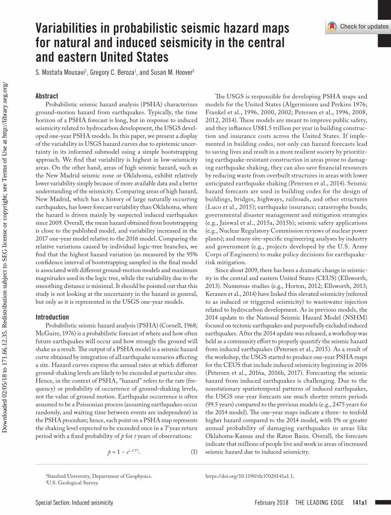
characterization (SSC) and ground-motion characterization (GMC). In SSC, the spatial and temporal models of earthquake recurrence are used to predict the distribution of future earthquakes of different magnitudes (Figure 1). In GMC, the ground-motion level is predicted at a particular site as a result of an earthquake
scenario. The information from SSC and GMC for all possible earthquake scenarios that may impact a site are combined using the total probability theorem to obtain the hazard curve for a site (Figure 1). It is important, however, to consider the uncertainties associated with calculated hazard curves.
Two types of uncertainties in the ontological framework of the PSHA procedure are aleatory and epistemic uncertainties (Kammerer and Ake, 2012).
Aleatory (also known as irreducible, inherent, stochastic, or type-A) uncertainty captures the inherent randomness in the natural system generating ground-shaking intensity. This uncer-tainty, classified as the known unknowns, explicitly refers to a particular model of nature used in the analysis and cannot be reduced. For instance, in the PSHA process, we might be able to determine the average recurrence rate for earthquakes of different magnitudes, but this does not mean we can predict the magnitude of the next earthquake. Aleatory uncertainty exists in the spatial model, temporal model, and empirical ground-motion prediction equations (GMPEs) that are used for GMC.
The second type of uncertainty in the PSHA process is the epistemic (also known as reducible, model, specification error, or type-B) uncertainty that reflects our limited knowledge of the parameters of a model describing earthquake processes. This uncertainty can be reduced by including more data and thereby improving our models. Epistemic uncertainties exist in every input to the PSHA process (e.g., selection of appropriate seismic-
ity catalog, GMPEs, or values of the maximum magnitude [Mmax]) and are often characterized using expert judg-ment about the reliability of inputs and model choices.
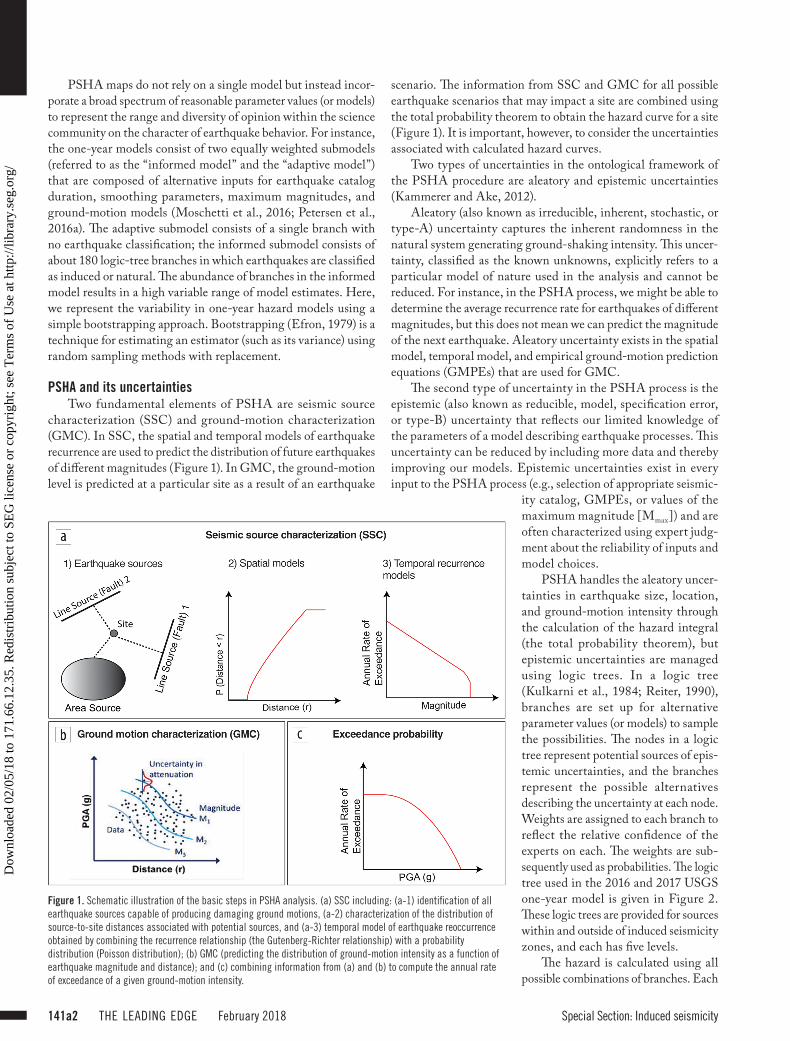
PSHA handles the aleatory uncer-tainties in earthquake size, location, and ground-motion intensity through the calculation of the hazard integral (the total probability theorem), but epistemic uncertainties are managed using logic trees. In a logic tree (Kulkarni et al., 1984; Reiter, 1990), branches are set up for alternative parameter values (or models) to sample the possibilities. The nodes in a logic tree represent potential sources of epis-temic uncertainties, and the branches represent the possible alternatives describing the uncertainty at each node. Weights are assigned to each branch to reflect the relative confidence of the experts on each. The weights are sub-sequently used as probabilities. The logic tree used in the 2016 and 2017 USGS one-year model is given in Figure 2. These logic trees are provided for sources within and outside of induced seismicity zones, and each has five levels.
The hazard is calculated using all possible combinations of branches. Each
Figure 1. Schematic illustration of the basic steps in PSHA analysis. (a) SSC including: (a-1) identification of all earthquake sources capable of producing damaging ground motions, (a-2) characterization of the distribution of source-to-site distances associated with potential sources, and (a-3) temporal model of earthquake reoccurrence obtained by combining the recurrence relationship (the Gutenberg-Richter relationship) with a probability distribution (Poisson distribution); (b) GMC (predicting the distribution of ground-motion intensity as a function of earthquake magnitude and distance); and (c) combining information from (a) and (b) to compute the annual rate of exceedance of a given ground-motion intensity.
Dow
nloa
ded
02/0
5/18
to 1
71.6
6.12
.35.
Red
istr
ibut
ion
subj
ect t
o SE
G li
cens
e or
cop
yrig
ht; s
ee T
erm
s of
Use
at h
ttp://
libra
ry.s
eg.o
rg/
February 2018 THE LEADING EDGE 141a3Special Section: Induced seismicity
individual combination of branches results in an individual hazard curve. There is a probability associated with each curve that is obtained by multiplication of the weights of all contributing branches. The final hazard estimate is calculated from a set of hazard curves obtained from a different combination of logic-tree branches, each associated with a probability (or weight). The aleatory variability influences the shape (gradient and curvature) of individual hazard curves, whereas the epistemic uncertainty gives rise to a suite of hazard curves. In Figure 3, we present the suite of individual curves, final model, and submodels from the 2016 forecast for Dallas, Texas.
In PSHA practice, some scientists describe the hazard using the percentiles of the logic-tree outcomes (e.g., Wang et al., 2003; Abrahamson and Bommer, 2005; Stucchi et al., 2011; Field et al., 2014). In the one-year models, only the mean hazards were reported, and engineers, regulators, and industry were advised to use the hazard forecasts cautiously for making informed decisions. This is attributable to another view among scientists that claims the use of percentiles discards probabilism and only the mean hazard should be interpreted (e.g., McGuire et al., 2005; Musson, 2005, 2012).
The importance of communicating the PSHA forecast with its center, body, and range, however — especially for a meaningful validation of the models — has been brought to attention in recent years (e.g., Marzocchi and Jordan, 2014). But using two submodels with a different number of branches and a wide range of individual curves (Figure 3) renders it difficult to represent the range of the hazard as the percentiles of the logic-tree outcomes. Moreover, Marzocchi et al. (2015) show that using percentiles violates the probability framework of the probability trees. Here, we use a simple bootstrapping approach to quantify the variability in estimated hazard by USGS one-year models. This might not reflect the ensemble uncertainty (as proposed in Marzocchi et al., 2015), but it does represent the relative degree of hazard estimate variability caused by expert evaluations of the actual reliability of the elements constituting the model.
MethodologyIt is common to use the distance between the 5th and 95th
percentile of unweighted hazard curves as an uncertainty metric for hazard models. Marzocchi et al. (2015) suggest that we may use the variability of the outcomes generated by a set of reasonable models to bound where the true hazard is expected to lie. This is consistent with the goal of quantifying epistemic uncertainty and is in agreement with the use of percentiles in the context of a logic tree.
Following this approach, we used logic-tree branches associ-ated with the informed submodel to quantify the variability in the final mode (mean hazard). The mean and 95% confidence interval of hazard for all ground-motion levels over the entire CEUS are calculated by bootstrapping (resampling with replace-ment) of the weighted branches of the logic tree. At each grid point and for each ground-motion level, we created 1000 hazard estimates by summing up resamples of 90% of the branches (annual rates of exceedances) of the informed submodel. The advantage of this approach over percentile calculation is that it incorporates the effects of assigned weights into the uncertainty estimation.
Variations of the mean hazards obtained by bootstrapping at each ground-motion level are used to calculate confidence interval.
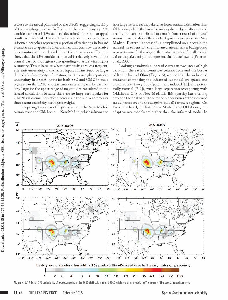
Results and discussionIn Figure 4b, peak horizontal ground acceleration (PGA)
levels associated with a fixed annual frequency of exceedance (1% probability of exceedance in one year) are plotted for the entire CEUS using the mean of bootstrapping samples for each site. The hazard map obtained from the mean of the bootstrapping samples
Figure 2. Logic tree used in the 2016 and 2017 one-year model for sites within defined zones of induced seismicity (top) and for sites outside of zones of induced seismicity (bottom).
Figure 3. Unweighted hazard curves associated with logic-tree branches (in black), the final hazard estimate, and submodels of the 2016 one-year model for Dallas. Informed submodel is obtained by summing weighted version of logic-tree branches (black lines).
Dow
nloa
ded
02/0
5/18
to 1
71.6
6.12
.35.
Red
istr
ibut
ion
subj
ect t
o SE
G li
cens
e or
cop
yrig
ht; s
ee T
erm
s of
Use
at h
ttp://
libra
ry.s
eg.o
rg/
141a4 THE LEADING EDGE February 2018 Special Section: Induced seismicity
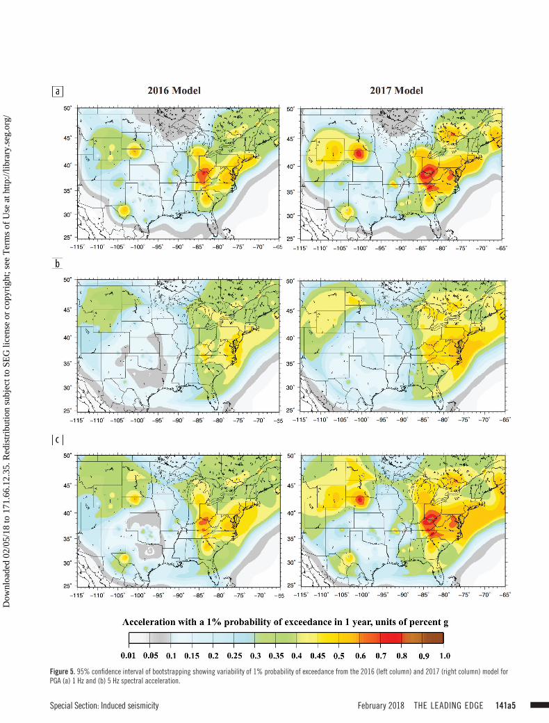
is close to the model published by the USGS, suggesting stability of the sampling process. In Figure 5, the accompanying 95% confidence interval (1.96 standard deviation) of the bootstrapped results is presented. The confidence interval of bootstrapped-informed branches represents a portion of variations in hazard estimates due to epistemic uncertainties. This can show the relative uncertainties in this submodel over the entire region. Figure 5 shows that the 95% confidence interval is relatively lower in the central part of the region corresponding to areas with higher seismicity. This is because where earthquakes are less frequent, epistemic uncertainty in the hazard inputs will inevitably be larger due to lack of seismicity information, resulting in higher epistemic uncertainty in PSHA inputs for both SSC and GMC in these regions. For the GMC, the epistemic uncertainty will be particu-larly large for the upper range of magnitudes considered in the hazard calculations because there are no large earthquakes for GMPE validation. This effect increases in the one-year forecasts since recent seismicity has higher weight.
Comparing two areas of high hazards — the New Madrid seismic zone and Oklahoma — New Madrid, which is known to
host large natural earthquakes, has lower standard deviation than Oklahoma, where the hazard is mainly driven by smaller induced events. This can be attributed to a much shorter record of induced seismicity in Oklahoma than for background seismicity near New Madrid. Eastern Tennessee is a complicated area because the natural treatment for the informed model has a background seismicity zone. In this region, the spatial patterns of small histori-cal earthquakes might not represent the future hazard (Petersen et al., 2008).
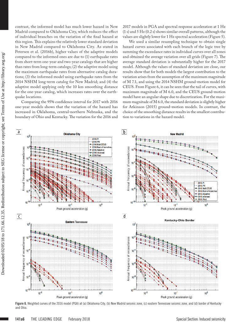
Looking at individual hazard curves in two areas of high variation, the eastern Tennessee seismic zone and the border of Kentucky and Ohio (Figure 6), we see that the individual branches composing the informed submodel are sparse and clustered into two groups (potentially induced [PI], and poten-tially natural [PN]), with large separation (comparing with Oklahoma City or New Madrid). This sparsity has a strong effect on the final hazard due to the higher values of the informed model (compared to the adaptive model) for these regions. On the other hand, for both New Madrid and Oklahoma, the adaptive rate models are higher than the informed model. In
Figure 4. (a) PGA for 1% probability of exceedance from the 2016 (left column) and 2017 (right column) model. (b) The mean of the bootstrapped samples.
Dow
nloa
ded
02/0
5/18
to 1
71.6
6.12
.35.
Red
istr
ibut
ion
subj
ect t
o SE
G li
cens
e or
cop
yrig
ht; s
ee T
erm
s of
Use
at h
ttp://
libra
ry.s
eg.o
rg/
February 2018 THE LEADING EDGE 141a5Special Section: Induced seismicity
Figure 5. 95% confidence interval of bootstrapping showing variability of 1% probability of exceedance from the 2016 (left column) and 2017 (right column) model for PGA (a) 1 Hz and (b) 5 Hz spectral acceleration.
Dow
nloa
ded
02/0
5/18
to 1
71.6
6.12
.35.
Red
istr
ibut
ion
subj
ect t
o SE
G li
cens
e or
cop
yrig
ht; s
ee T
erm
s of
Use
at h
ttp://
libra
ry.s
eg.o
rg/
141a6 THE LEADING EDGE February 2018 Special Section: Induced seismicity
contrast, the informed model has much lower hazard in New Madrid compared to Oklahoma City, which reduces the effect of individual branches on the variation of the final hazard at this region. This explains the relatively lower standard deviation in New Madrid compared to Oklahoma City. As stated in Petersen et al. (2016b), higher values of the adaptive models compared to the informed ones are due to (1) earthquake rates from short-term one-year and two-year catalogs that are higher than rates from long-term catalogs; (2) the adaptive model using the maximum earthquake rates from alternative catalog dura-tions; (3) the informed model using earthquake rates from the 2014 NSHM long-term catalog for New Madrid; and (4) the adaptive model applying only the 10 km smoothing distance for the one-year catalog, which increases rates over the earth-quake locations.
Comparing the 95% confidence interval for 2017 with 2016 one-year models shows that the variation of the hazard has increased in Oklahoma, central-northern Nebraska, and the boundary of Ohio and Kentucky. The variation for the 2016 and
2017 models in PGA and spectral response acceleration at 1 Hz (1 s) and 5 Hz (0.2 s) shows similar overall patterns, although the values are slightly lower for 1 Hz spectral acceleration (Figure 5).
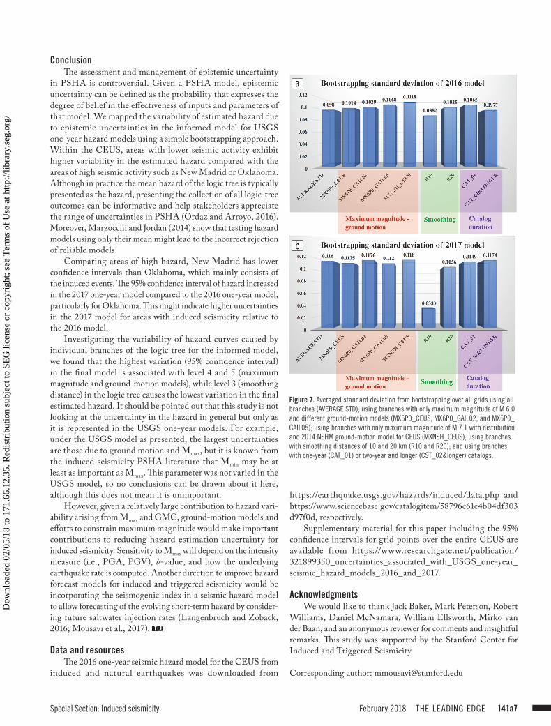
We used a similar resampling technique to obtain single hazard curves associated with each branch of the logic tree by summing the exceedance rates in individual curves over all zones and obtained the average variation over all grids (Figure 7). The average standard deviation is substantially higher for the 2017 model. Although the values of standard deviation are close, our results show that for both models the largest contribution to the variation arises from the assumption of the maximum magnitude of M 7.1, and using the 2014 NSHM ground-motion model for CEUS. From Figure 6, it can be seen that the tail of curves, with maximum magnitude of M 6.0, and the CEUS ground-motion model have an angular shape due to discretization. For the maxi-mum magnitude of M 6.0, the standard deviation is slightly higher for Atkinson (2015) ground-motion models. In contrast, the choice of the smoothing distance results in the smallest contribu-tion to variations in the hazard model.
Figure 6. Weighted curves of the 2016 model (PGA) at (a) Oklahoma City, (b) New Madrid seismic zone, (c) eastern Tennessee seismic zone, and (d) border of Kentucky and Ohio.
Dow
nloa
ded
02/0
5/18
to 1
71.6
6.12
.35.
Red
istr
ibut
ion
subj
ect t
o SE
G li
cens
e or
cop
yrig
ht; s
ee T
erm
s of
Use
at h
ttp://
libra
ry.s
eg.o
rg/
February 2018 THE LEADING EDGE 141a7Special Section: Induced seismicity
ConclusionThe assessment and management of epistemic uncertainty
in PSHA is controversial. Given a PSHA model, epistemic uncertainty can be defined as the probability that expresses the degree of belief in the effectiveness of inputs and parameters of that model. We mapped the variability of estimated hazard due to epistemic uncertainties in the informed model for USGS one-year hazard models using a simple bootstrapping approach. Within the CEUS, areas with lower seismic activity exhibit higher variability in the estimated hazard compared with the areas of high seismic activity such as New Madrid or Oklahoma. Although in practice the mean hazard of the logic tree is typically presented as the hazard, presenting the collection of all logic-tree outcomes can be informative and help stakeholders appreciate the range of uncertainties in PSHA (Ordaz and Arroyo, 2016). Moreover, Marzocchi and Jordan (2014) show that testing hazard models using only their mean might lead to the incorrect rejection of reliable models.
Comparing areas of high hazard, New Madrid has lower confidence intervals than Oklahoma, which mainly consists of the induced events. The 95% confidence interval of hazard increased in the 2017 one-year model compared to the 2016 one-year model, particularly for Oklahoma. This might indicate higher uncertainties in the 2017 model for areas with induced seismicity relative to the 2016 model.
Investigating the variability of hazard curves caused by individual branches of the logic tree for the informed model, we found that the highest variation (95% confidence interval) in the final model is associated with level 4 and 5 (maximum magnitude and ground-motion models), while level 3 (smoothing distance) in the logic tree causes the lowest variation in the final estimated hazard. It should be pointed out that this study is not looking at the uncertainty in the hazard in general but only as it is represented in the USGS one-year models. For example, under the USGS model as presented, the largest uncertainties are those due to ground motion and Mmax, but it is known from the induced seismicity PSHA literature that Mmin may be at least as important as Mmax. This parameter was not varied in the USGS model, so no conclusions can be drawn about it here, although this does not mean it is unimportant.
However, given a relatively large contribution to hazard vari-ability arising from Mmax and GMC, ground-motion models and efforts to constrain maximum magnitude would make important contributions to reducing hazard estimation uncertainty for induced seismicity. Sensitivity to Mmax will depend on the intensity measure (i.e., PGA, PGV), b-value, and how the underlying earthquake rate is computed. Another direction to improve hazard forecast models for induced and triggered seismicity would be incorporating the seismogenic index in a seismic hazard model to allow forecasting of the evolving short-term hazard by consider-ing future saltwater injection rates (Langenbruch and Zoback, 2016; Mousavi et al., 2017).
Data and resourcesThe 2016 one-year seismic hazard model for the CEUS from
induced and natural earthquakes was downloaded from
https://earthquake.usgs.gov/hazards/induced/data.php and https://www.sciencebase.gov/catalogitem/58796c61e4b04df303d97f0d, respectively.
Supplementary material for this paper including the 95% confidence intervals for grid points over the entire CEUS are available from https://www.researchgate.net/publication/ 321899350_uncertainties_associated_with_USGS_one-year_seismic_hazard_models_2016_and_2017.
AcknowledgmentsWe would like to thank Jack Baker, Mark Peterson, Robert
Williams, Daniel McNamara, William Ellsworth, Mirko van der Baan, and an anonymous reviewer for comments and insightful remarks. This study was supported by the Stanford Center for Induced and Triggered Seismicity.
Corresponding author: [email protected]
Figure 7. Averaged standard deviation from bootstrapping over all grids using all branches (AVERAGE STD); using branches with only maximum magnitude of M 6.0 and different ground-motion models (MX6P0_CEUS, MX6P0_GAIL02, and MX6P0_GAIL05); using branches with only maximum magnitude of M 7.1 with distribution and 2014 NSHM ground-motion model for CEUS (MXNSH_CEUS); using branches with smoothing distances of 10 and 20 km (R10 and R20); and using branches with one-year (CAT_01) or two-year and longer (CST_02&longer) catalogs.
Dow
nloa
ded
02/0
5/18
to 1
71.6
6.12
.35.
Red
istr
ibut
ion
subj
ect t
o SE
G li
cens
e or
cop
yrig
ht; s
ee T
erm
s of
Use
at h
ttp://
libra
ry.s
eg.o
rg/
141a8 THE LEADING EDGE February 2018 Special Section: Induced seismicity
ReferencesAbrahamson, N. A., and J. J. Bommer, 2005, Probability and uncer-
tainty in seismic hazard analysis: Earthquake Spectra, 21, no. 2, 603–607, https://doi.org/10.1193/1.1899158.
Algermissen, S. T., and D. M. Perkins, 1976, A probabilistic esti-mate of the maximum acceleration in rock in the contiguous United States: U.S. Geological Survey Open-File Report 76-416.
Atkinson, G. M., 2015, Ground-motion prediction equation for small-to-moderate events at short hypocentral distances, with application to induced seismicity hazards: Bulletin of the Seis-mological Society of America, 105, no. 2A, 981–992, https://doi.org/10.1785/0120140142.
Cornell, C. A., 1968, Engineering seismic risk analysis: Bulletin of the Seismological Society of America, 58, 1583–1606.
Efron, B., 1979, Bootstrap methods: Another look at jackknife: Annals of Statistics, 7, no. 1, 1–26, https://doi.org/10.1214/aos/1176344552.
Ellsworth, W. L., 2013, Injection-induced earthquakes: Science, 341, no. 6142, https://doi.org/10.1126/science.1225942.
Field, E. H․, R. J. Arrowsmith, G. P. Biasi, P. Bird, T. E. Dawson, K. R. Felzer, D. D. Jackson, et al., 2014, Uniform California earth-quake rupture forecast, version 3 (UCERF3) — The time-inde-pendent model: Bulletin of the Seismological Society of Amer-ica, 104, no. 3, 1122–1180, https://doi.org/10.1785/0120130164.
Frankel, A., C. Mueller, T. Barnhard, D. Perkins, E. V. Leyendecker, N. Dickman, S. Hanson, and M. Hopper, 1996, National seis-mic hazard maps — Documentation June 1996: U.S. Geological Survey Open-File Report.
Frankel, A. D., C. S. Mueller, T. P. Barnhard, E. V. Leyendecker, R. L. Wesson, S. C. Harmsen, F. W. Klein, et al., 2000, USGS national seismic hazard maps: Earthquake Spectra, 16, no. 1, 1–19, https://doi.org/10.1193/1.1586079.
Frankel, A. D., M. D. Petersen, C. S. Mueller, K. M. Haller, R. L. Wheeler, E. V. Leyendecker, R. L. Wesson, et al., 2002, Docu-mentation for the 2002 update of the national seismic hazard maps: U.S. Geological Survey Open-File Report.
Horton, S., 2012, Disposal of hydrofracking waste fluid by injection into subsurface aquifers triggers earthquake swarm in central Arkan-sas with potential for damaging earthquake: Seismological Research Letters, 83, no. 2, 250–260, https://doi.org/10.1785/gssrl.83.2.250.
Jaiswal, K. S., M. D. Petersen, K. Rukstales, and W. S. Leith, 2015a, Earthquake shaking hazard estimates and exposure changes in the conterminous United States: Earthquake Spectra, 31, no. S1, S201–S220, https://doi.org/10.1193/111814EQS195M.
Jaiswal, K. S., D. Bausch, R. Chen, J. Bouabid, and H. Seligson, 2015b, Estimating annualized earthquake losses for the conter-minous United States: Earthquake Spectra, 31, no. S1, S221–S243, https://doi.org/10.1193/010915EQS005M.
Kammerer, A. M., and J. P. Ake, 2012, Practical implementation guidelines for SSHAC level 3 and 4 hazard studies (NUREG-2117, Revision 1): Office of Nuclear Regulatory Research.
Keranen, K. M., M. Weingarten, G. A. Abers, B. A. Bekins, and S. Ge, 2014, Sharp increase in central Oklahoma seismicity since 2008 induced by massive wastewater injection: Science, 345, no. 6195, 448–451, https://doi.org/10.1126/science.1255802.
Kulkarni, R. B., R. R. Youngs, and K. J. Coppersmith, 1984, Assess-ment of confidence intervals for results of seismic hazard analy-sis: Proceedings of the 8th World Conference on Earthquake Engi-neering, 1, 263–270.
Langenbruch, C., and M. D. Zoback, 2016, How will induced seis-micity in Oklahoma respond to decreased saltwater injection rates?: Science Advances, 2, no. 11, https://doi.org/10.1126/sciadv.1601542.
Luco, N., R. E. Bachman, C. B. Crouse, J. R. Harris, J. D. Hooper, C. A. Kircher, P. J. Caldwell, and K. R. Rukstales, 2015, Updates to building-code maps for the 2015 NEHRP recommended seis-mic provisions: Earthquake Spectra, 31, no. S1, S245–S271, https://doi.org/10.1193/042015EQS058M.
Marzocchi, W., and T. H. Jordan, 2014, Testing for ontological errors in probabilistic forecasting models of natural systems: Proceed-ings of the National Academy of Sciences of the United States of America, 111, no. 33, 11973–11978, https://doi.org/10.1073/pnas.1410183111.
Marzocchi, W., M. Taroni, and J. Selva, 2015, Accounting for epis-temic uncertainty in PSHA — Logic tree and ensemble model-ing: Bulletin of the Seismological Society of America, 105, no. 4, 2151–2159, https://doi.org/10.1785/0120140131.
McGuire, R. K., 1976, FORTRAN computer program for seismic risk analysis: U.S. Geological Survey Open-File Report.
McGuire, R. K., C. A. Cornell, and G. R. Toro, 2005, The case for using mean seismic hazard: Earthquake Spectra, 21, no. 3, 879–886, https://doi.org/10.1193/1.1985447.
Moschetti, M. P., S. M. Hoover, and C. S. Mueller, 2016, Likeli-hood testing of seismicity-based rate forecasts of induced earth-quakes in Oklahoma and Kansas: Geophysical Research Letters, 43, no. 10, 4913–4921, https://doi.org/10.1002/2016GL068948.
Mousavi, S. M., S. Horton, P. Ogwari, and C. A. Langston, 2017, Spatio-temporal evolution of frequency-magnitude distribution and seismogenic index during initiation of induced seismicity at Guy-Greenbrier, Arkansas: Physics of the Earth and Planetary Interiors, 267, 53–66, https://doi.org/10.1016/j.pepi.2017.04.005.
Musson, R. M. W., 2005, Against fractiles: Earthquake Spectra, 21, no. 3, 887–891, https://doi.org/10.1193/1.1985445.
Musson, R. M. W., 2012, On the nature of logic trees in probabi-listic seismic hazard assessment: Earthquake Spectra, 28, no. 3, 1291–1296, https://doi.org/10.1193/1.4000062.
Ordaz, M., and D. Arroyo, 2016, On uncertainties in probabilistic seismic hazard analysis: Earthquake Spectra, 32, no. 3, 1405–1418, https://doi.org/10.1193/052015EQS075M.
Petersen, M. D., W. A. Bryant, C. H. Cramer, T. Cao, and M. Reichle, 1996, Probabilistic seismic hazard assessment for the State of California: California Geological Survey, Open-File Report 96-08 and U.S. Geological Survey Open-File Report 96-706.
Petersen, M. D., A. D. Frankel, S. C. Harmsen, C. S. Mueller, K. M. Haller, R. L. Wheeler, R. L. Wesson, et al., 2008, Doc-umentation for the 2008 update of the United States national seismic hazard maps: U.S. Geological Survey Open-File Report 2008-1128.
Petersen, M. D., A. D. Frankel, S. C. Harmsen, and C. S. Mueller, O. S., Boyd, N. Luco, R. L. Wheeler, K. S. Rukstales, and K. M. Haller, 2012, The 2008 U.S. Geological Survey national seismic hazard models and maps for the central and eastern United States, in R. T. Cox, M. P. Tuttle, O. S. Boyd, and J. Locat, eds., Recent advances in North American paleoseismology and neotectonics east of the Rockies: Geological Society of America, 243–257, https://doi.org/10.1130/2012.2493(12).
Petersen, M. D., M. P. Moschetti, P. M. Powers, C. S. Mueller, K. M. Haller, A. D. Frankel, Y. Zeng, S. Rezaeian, S. C. Harmsen, O. S. Boyd, et al., 2014, Documentation for the 2014 update of the United States national seismic hazard maps: U.S. Geological Sur-vey Open-File Report 2014-1091, https://doi.org/10.3133/ofr20141091.
Petersen, M. D., C. S. Mueller, M. P. Moschetti, S. M. Hoover, J. L. Rubinstein, A. L. Llenos, A. J. Michael, et al., 2015,
Dow
nloa
ded
02/0
5/18
to 1
71.6
6.12
.35.
Red
istr
ibut
ion
subj
ect t
o SE
G li
cens
e or
cop
yrig
ht; s
ee T
erm
s of
Use
at h
ttp://
libra
ry.s
eg.o
rg/

February 2018 THE LEADING EDGE 141a9Special Section: Induced seismicity
Incorporating induced seismicity in the 2014 United States national seismic hazard model — Results of 2014 workshop and sensitiv-ity studies: U.S. Geological Survey Open-File Report 2015-1070, https://doi.org/10.3133/ofr20151070.
Petersen, M. D., C. S. Mueller, M. P. Moschetti, S. M. Hoover, A. L. Llenos, W. L. Ellsworth, A. J. Michael, J. L. Rubinstein, A. F. McGarr, and K. S. Rukstales, 2016a, 2016 one-year seismic haz-ard forecast for the central and eastern United States from induced and natural earthquakes: U.S. Geological Survey Open-File Report 2016-1035, https://doi.org/10.3133/ofr20161035.
Petersen, M. D., C. S. Mueller, M. P. Moschetti, S. M. Hoover, A. L. Llenos, W. L. Ellsworth, A. J. Michael, J. L. Rubinstein, A. F. McGarr, and K. S. Rukstales, 2016b, Seismic-hazard fore-cast for 2016 including induced and natural earthquakes in the central and eastern United States: Seismological Research Let-ters, 87, no. 6, 1327–1341, https://doi.org/10.1785/0220160072.
Petersen, M. D., C. S. Mueller, M. P. Moschetti, S. M. Hoover, A. M. Shumway, D. E. McNamara, R. A. Williams, et al., 2017, One-year seismic-hazard forecast for the central and eastern United States from induced and natural earthquakes: Seismo-logical Research Letters, 88, no. 3, 772–783, https://doi.org/10.1785/0220170005.
Reiter, L., 1990, Earthquake hazard analysis — Issues and insights: Columbia University Press.
Stucchi, M., C. Meletti, V. Montaldo, H. Crowley, G. M. Calvi, and E. Boschi, 2011, Seismic hazard assessment (2003–2009) for the Italian Building Code: Bulletin of the Seismological Society of Amer-ica, 101, no. 4, 1885–1911, https://doi.org/10.1785/0120100130.
Wang, Z., E. W. Woolery, B. Shi, and J. D. Kiefer, 2003, Commu-nicating with uncertainty: A critical issue with probabilistic seis-mic hazard analysis: EOS, 84, no. 46, 501–508, https://doi.org/10.1029/2003EO460002.
Dow
nloa
ded
02/0
5/18
to 1
71.6
6.12
.35.
Red
istr
ibut
ion
subj
ect t
o SE
G li
cens
e or
cop
yrig
ht; s
ee T
erm
s of
Use
at h
ttp://
libra
ry.s
eg.o
rg/