Variability –Waiting Times - Augusta Universityspots.gru.edu/jgrayson/MBAOpsMgt/CachonMSWDCurrentLectureSlides...QUAN6610 Prepared by Jim Grayson, PhD 1 Variability –Waiting Times

QUAN6610

Prepared by Jim Grayson, PhD 1

Variability – Waiting Times

Chapter 8Matching Supply with Demand, 3e

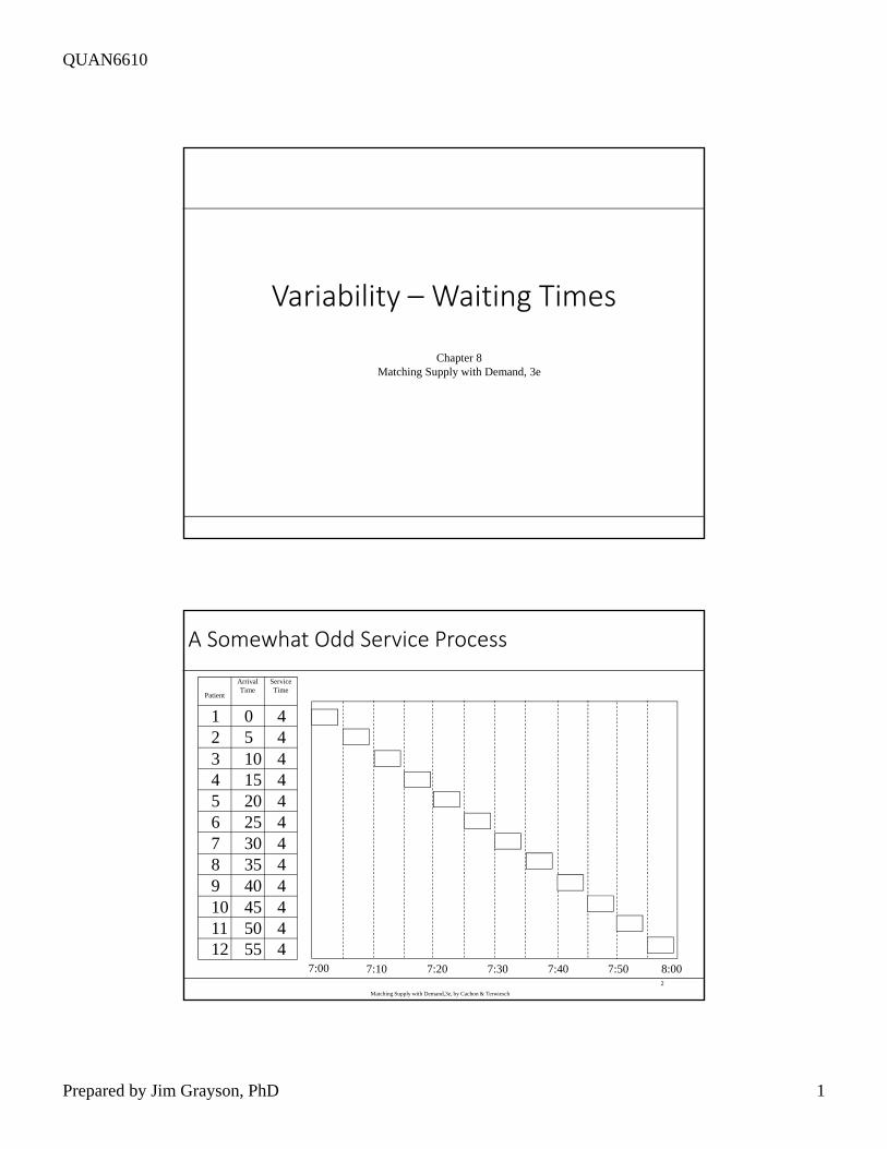
7:00 7:10 7:20 7:30 7:40 7:50 8:00

Patient

ArrivalTime

ServiceTime

123456789101112

0510152025303540455055

444444444444

A Somewhat Odd Service Process

2

Matching Supply with Demand,3e, by Cachon & Terwiesch

QUAN6610


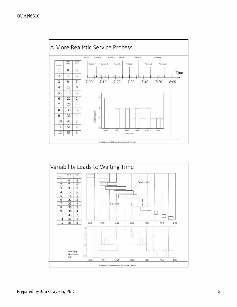
Patient

ArrivalTime

ServiceTime

1

2

3

4

5

6

7

8

9

10

11

12

0

7

9

12

18

22

25

30

36

45

51

55

5

6

7

6

5

2

4

3

4

2

2

3

Time

7:10 7:20 7:30 7:40 7:50 8:007:00

Patient 1 Patient 3 Patient 5 Patient 7 Patient 9 Patient 11

Patient 2 Patient 4 Patient 6 Patient 8 Patient 10 Patient 12

0

1

2

3

2 min. 3 min. 4 min. 5 min. 6 min. 7 min.

Service times

Num

ber

of c

ases

A More Realistic Service Process

3


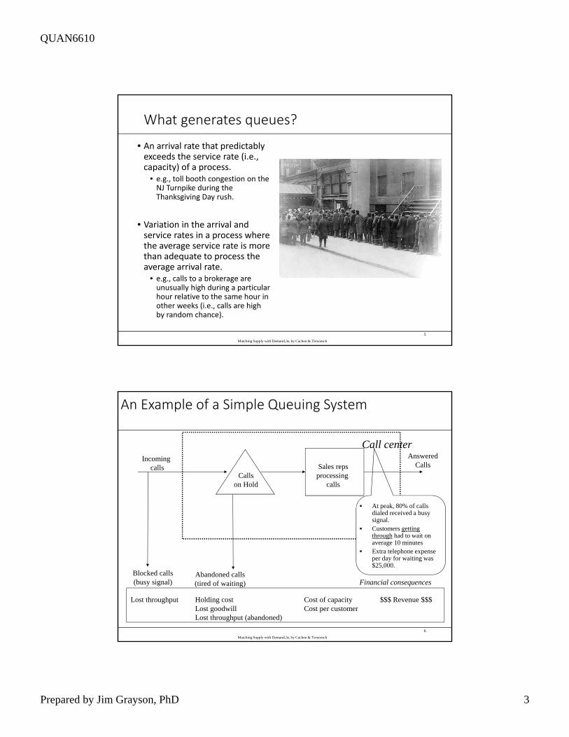
7:00 7:10 7:20 7:30 7:40 7:50

Inventory(Patients atlab)

5

4

3

2

1

0

8:00

7:00 7:10 7:20 7:30 7:40 7:50 8:00

Wait time

Service time

Patient

ArrivalTime

ServiceTime

123456789101112

079121822253036455155

567652434223

Variability Leads to Waiting Time

4


QUAN6610


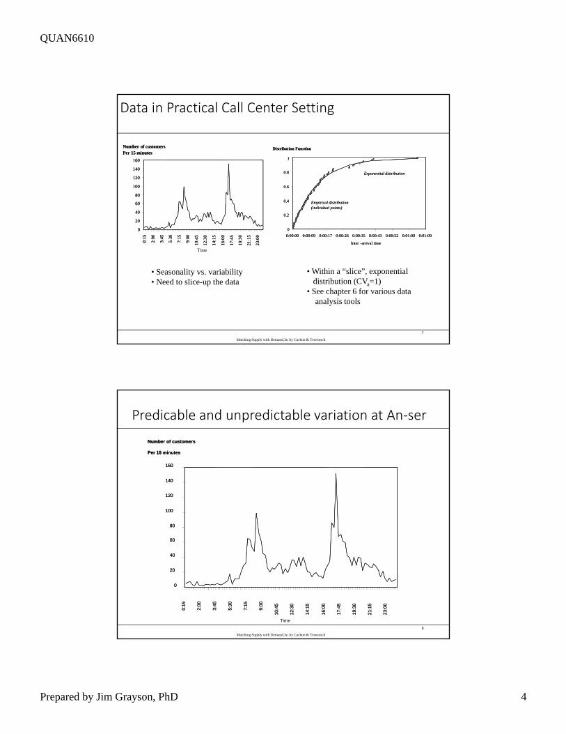
What generates queues?

• An arrival rate that predictably exceeds the service rate (i.e., capacity) of a process.

• e.g., toll booth congestion on the NJ Turnpike during the Thanksgiving Day rush.

• Variation in the arrival and service rates in a process where the average service rate is more than adequate to process the average arrival rate.

• e.g., calls to a brokerage are unusually high during a particular hour relative to the same hour in other weeks (i.e., calls are high by random chance).

5


Blocked calls(busy signal)

Abandoned calls(tired of waiting)

Callson Hold

Sales repsprocessing

calls

AnsweredCalls

Incoming calls

Call center

Financial consequences

Lost throughput Holding costLost goodwillLost throughput (abandoned)

$$$ Revenue $$$Cost of capacityCost per customer

At peak, 80% of calls dialed received a busy signal.

Customers getting through had to wait on average 10 minutes

Extra telephone expense per day for waiting was $25,000.

An Example of a Simple Queuing System

6


QUAN6610


0

20

40

60

80

100

120

140

160

0:15

2:00

3:45

5:30

7:15

9:00

10:4

5

12:3

0

14:1

5

16:0

0

17:4

5

19:3

0

21:1

5

23:0

0

Number of customersPer 15 minutes

0

20

40

60

80

100

120

140

160

0:15

2:00

3:45

5:30

7:15

9:00

10:4

5

12:3

0

14:1

5

16:0

0

17:4

5

19:3

0

21:1

5

23:0

0

Time

Number of customersPer 15 minutes

0

0.2

0.4

0.6

0.8

1

0:00:00 0:00:09 0:00:17 0:00:26 0:00:35 0:00:43 0:00:52 0:01:00 0:01:09

Distribution Function

Empirical distribution(individual points)

Exponential distribution

0

0.2

0.4

0.6

0.8

1

0:00:00 0:00:09 0:00:17 0:00:26 0:00:35 0:00:43 0:00:52 0:01:00 0:01:09

Distribution Function

Inter -arrival timeInter -arrival time

Empirical distribution(individual points)

Exponential distribution

• Seasonality vs. variability• Need to slice-up the data

• Within a “slice”, exponential distribution (CVa=1)

• See chapter 6 for various dataanalysis tools

Data in Practical Call Center Setting

7


Predicable and unpredictable variation at An‐ser

0

20

40

60

80

100

120

140

160

0:15

2:00

3:45

5:30

7:15

9:00

10:4

5

12:3

0

14:1

5

16:0

0

17:4

5

19:3

0

21:1

5

23:0

0

Number of customers

Per 15 minutes

0

20

40

60

80

100

120

140

160

0:15

2:00

3:45

5:30

7:15

9:00

10:4

5

12:3

0

14:1

5

16:0

0

17:4

5

19:3

0

21:1

5

23:0

0

Time

Number of customers

Per 15 minutes

8


QUAN6610


Defining inter‐arrival times and a stationary process

• An inter‐arrival time is the amount of time between two arrivals to a process.

• An arrival process is stationary over a period of time if the number of arrivals in any sub‐interval depends only on the length of the interval and not on when the interval starts.

• For example, if the process is stationary over the course of a day, then the expected number of arrivals within any three hour interval is about the same no matter which three hour window is chosen (or six hour window, or one hour window, etc).

• Processes tend to be non‐stationary (or seasonal) over long time periods (e.g., over a day or several hours) but stationary over short periods of time (say one hour, or 15 minutes).

9


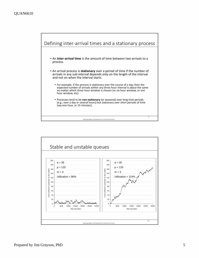
Stable and unstable queues

a = 35

p = 120

m = 4

Utilization = 86%

a = 35

p = 120

m = 3

Utilization = 114%

10


QUAN6610


Arrivals to An‐ser over the day are non‐stationary

0

20

40

60

80

100

120

140

160

0:15

2:00

3:45

5:30

7:15

9:00

10:4

5

12:3

0

14:1

5

16:0

0

17:4

5

19:3

0

21:1

5

23:0

0

Number of customers

Per 15 minutes

0

20

40

60

80

100

120

140

160

0:15

2:00

3:45

5:30

7:15

9:00

10:4

5

12:3

0

14:1

5

16:0

0

17:4

5

19:3

0

21:1

5

23:0

0

Time

Number of customers

Per 15 minutesThe number of arrivals

in a 3-hour interval clearly depends on

which 3-hour interval your choose …

… and the peaks and troughs are predictable (they

occur roughly at the same time each day.

11


How to describe (or model) inter‐arrival times

• We will use two parameters to describe inter‐arrival times to a process:

• The average inter‐arrival time.

• The standard deviation of the inter‐arrival times.

• What is the standard deviation?

• Roughly speaking, the standard deviation is a measure of how variable the inter‐arrival times are.

• Two arrival processes can have the same average inter‐arrival time (say 1 minute) but one can have more variation about that average, i.e., a higher standard deviation.

12


QUAN6610


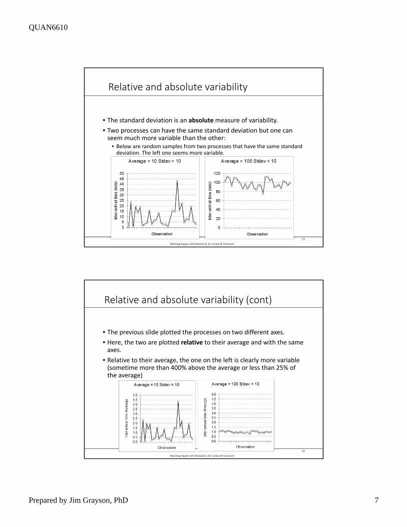
Relative and absolute variability

• The standard deviation is an absolutemeasure of variability.

• Two processes can have the same standard deviation but one can seem much more variable than the other:

• Below are random samples from two processes that have the same standard deviation. The left one seems more variable.

13


Relative and absolute variability (cont)

• The previous slide plotted the processes on two different axes.

• Here, the two are plotted relative to their average and with the same axes.

• Relative to their average, the one on the left is clearly more variable (sometime more than 400% above the average or less than 25% of the average)

14


QUAN6610


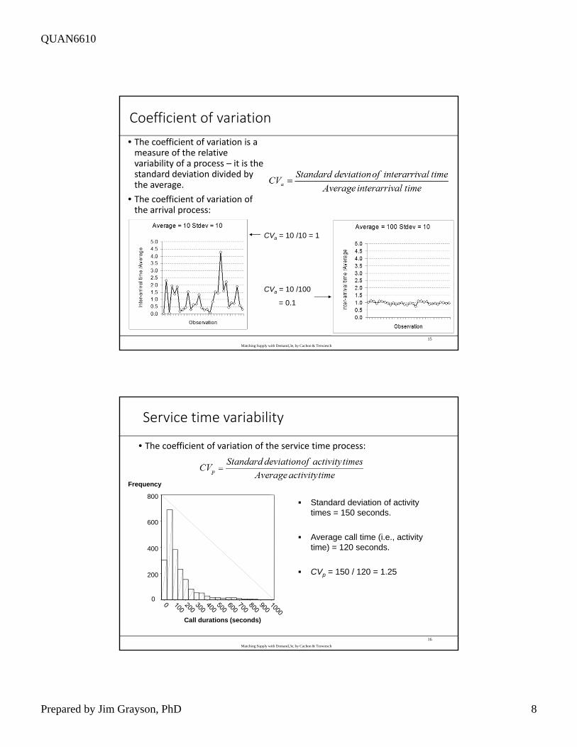
Coefficient of variation

• The coefficient of variation is a measure of the relative variability of a process – it is the standard deviation divided by the average.

• The coefficient of variation of the arrival process:

CVa = 10 /10 = 1

CVa = 10 /100

= 0.1

15


Service time variability

• The coefficient of variation of the service time process:

800

600

400

200

0

Call durations (seconds)

Frequency

Standard deviation of activity times = 150 seconds.

Average call time (i.e., activity time) = 120 seconds.

CVp = 150 / 120 = 1.25

16


QUAN6610


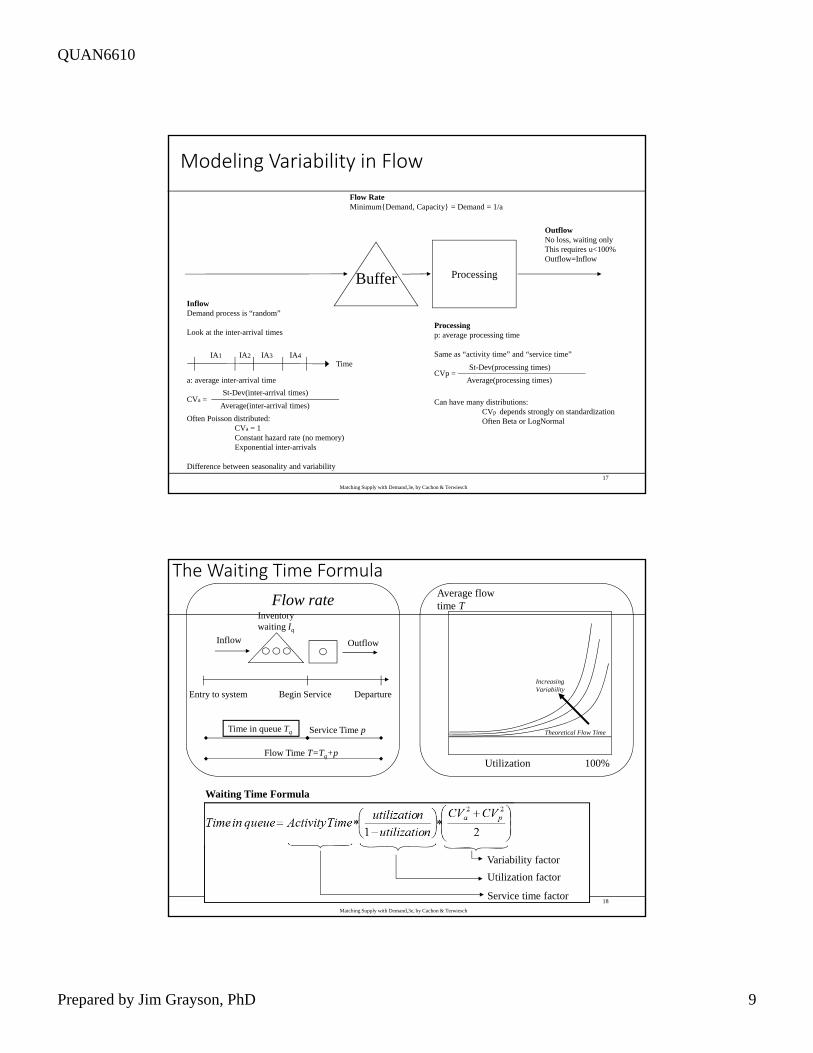
Processing

Modeling Variability in Flow

InflowDemand process is “random”

Look at the inter-arrival times

a: average inter-arrival time

CVa =

Often Poisson distributed:CVa = 1Constant hazard rate (no memory)Exponential inter-arrivals

Difference between seasonality and variability

Buffer

St-Dev(inter-arrival times)

Average(inter-arrival times)

TimeIA1 IA2 IA3 IA4

Processingp: average processing time

Same as “activity time” and “service time”

CVp =

Can have many distributions:CVp depends strongly on standardizationOften Beta or LogNormal

St-Dev(processing times)

Average(processing times)

OutflowNo loss, waiting onlyThis requires u<100%Outflow=Inflow

Flow RateMinimum{Demand, Capacity} = Demand = 1/a

17


Average flowtime T

Theoretical Flow Time

Utilization 100%

Increasing Variability

Waiting Time Formula

Service time factor

Utilization factor

Variability factor

Inflow Outflow

Inventorywaiting Iq

Entry to system DepartureBegin Service

Time in queue Tq Service Time p

Flow Time T=Tq+p

Flow rate

The Waiting Time Formula

18


QUAN6610


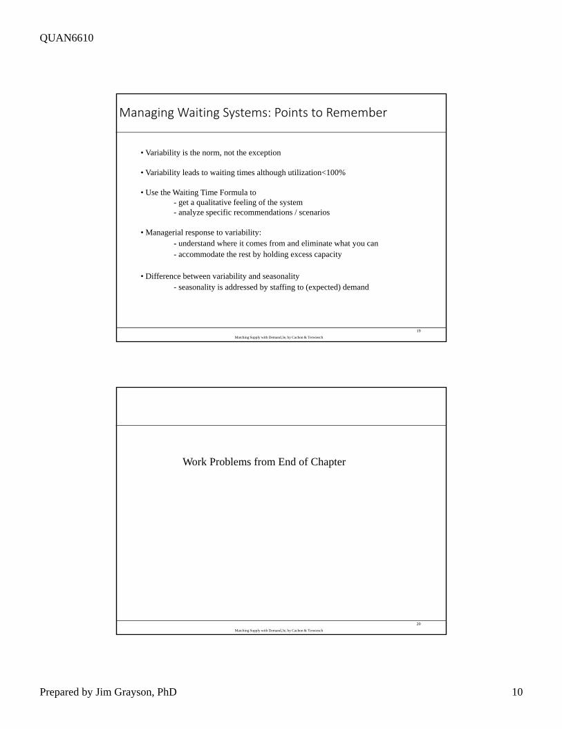
• Variability is the norm, not the exception

• Variability leads to waiting times although utilization<100%

• Use the Waiting Time Formula to- get a qualitative feeling of the system- analyze specific recommendations / scenarios

• Managerial response to variability:- understand where it comes from and eliminate what you can- accommodate the rest by holding excess capacity

• Difference between variability and seasonality- seasonality is addressed by staffing to (expected) demand

Managing Waiting Systems: Points to Remember

19


Work Problems from End of Chapter

20


QUAN6610


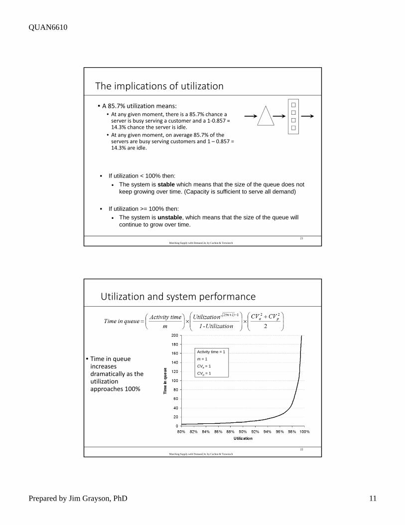
The implications of utilization

• A 85.7% utilization means:• At any given moment, there is a 85.7% chance a server is busy serving a customer and a 1‐0.857 = 14.3% chance the server is idle.

• At any given moment, on average 85.7% of the servers are busy serving customers and 1 – 0.857 = 14.3% are idle.

If utilization < 100% then:

The system is stable which means that the size of the queue does not keep growing over time. (Capacity is sufficient to serve all demand)

If utilization >= 100% then:

The system is unstable, which means that the size of the queue will continue to grow over time.

21


Utilization and system performance

• Time in queue increases dramatically as the utilization approaches 100%

Activity time = 1

m = 1

CVa = 1

CVp = 1

22


QUAN6610


Multiple Servers

23


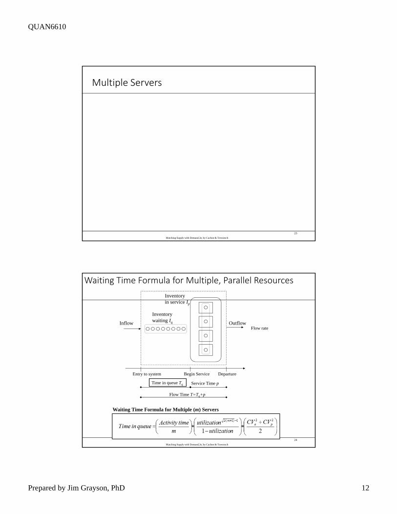
Waiting Time Formula for Multiple (m) Servers

Inflow Outflow

Inventorywaiting Iq



Flow Time T=Tq+p

Inventoryin service Ip

Flow rate

Waiting Time Formula for Multiple, Parallel Resources

24


QUAN6610


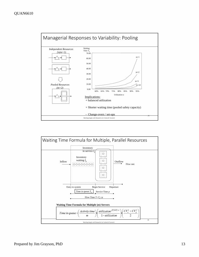
Independent Resources 2x(m=1)

Pooled Resources(m=2)

0.00

10.00

20.00

30.00

40.00

50.00

60.00

70.00

60% 65%

m=1

m=2

m=5

m=10

70% 75% 80% 85% 90% 95%

Waiting Time Tq

Utilization uImplications:+ balanced utilization

+ Shorter waiting time (pooled safety capacity)

- Change-overs / set-ups

Managerial Responses to Variability: Pooling

25


Waiting Time Formula for Multiple (m) Servers

Inflow Outflow

Inventorywaiting Iq



Flow Time T=Tq+p

Inventoryin service Ip

Flow rate

Waiting Time Formula for Multiple, Parallel Resources

26


QUAN6610


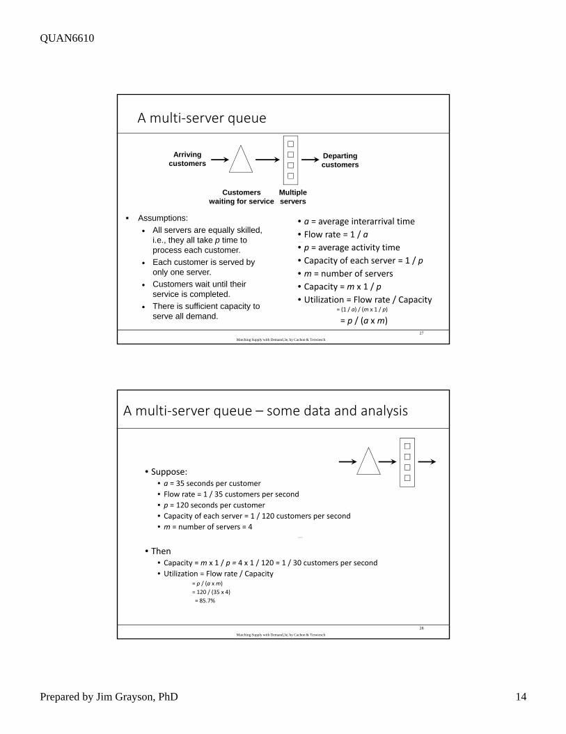
A multi‐server queue

• a = average interarrival time

• Flow rate = 1 / a• p = average activity time

• Capacity of each server = 1 / p• m = number of servers

• Capacity = m x 1 / p

• Utilization = Flow rate / Capacity= (1 / a) / (m x 1 / p)

= p / (a x m)

Multiple servers

Customers waiting for service

Arriving customers

Departing customers

Assumptions:

All servers are equally skilled, i.e., they all take p time to process each customer.

Each customer is served by only one server.

Customers wait until their service is completed.

There is sufficient capacity to serve all demand.

27


A multi‐server queue – some data and analysis

• Suppose:• a = 35 seconds per customer

• Flow rate = 1 / 35 customers per second

• p = 120 seconds per customer

• Capacity of each server = 1 / 120 customers per second

• m = number of servers = 4

• Then • Capacity = m x 1 / p = 4 x 1 / 120 = 1 / 30 customers per second

• Utilization = Flow rate / Capacity= p / (a x m)

= 120 / (35 x 4)

= 85.7%

28


QUAN6610


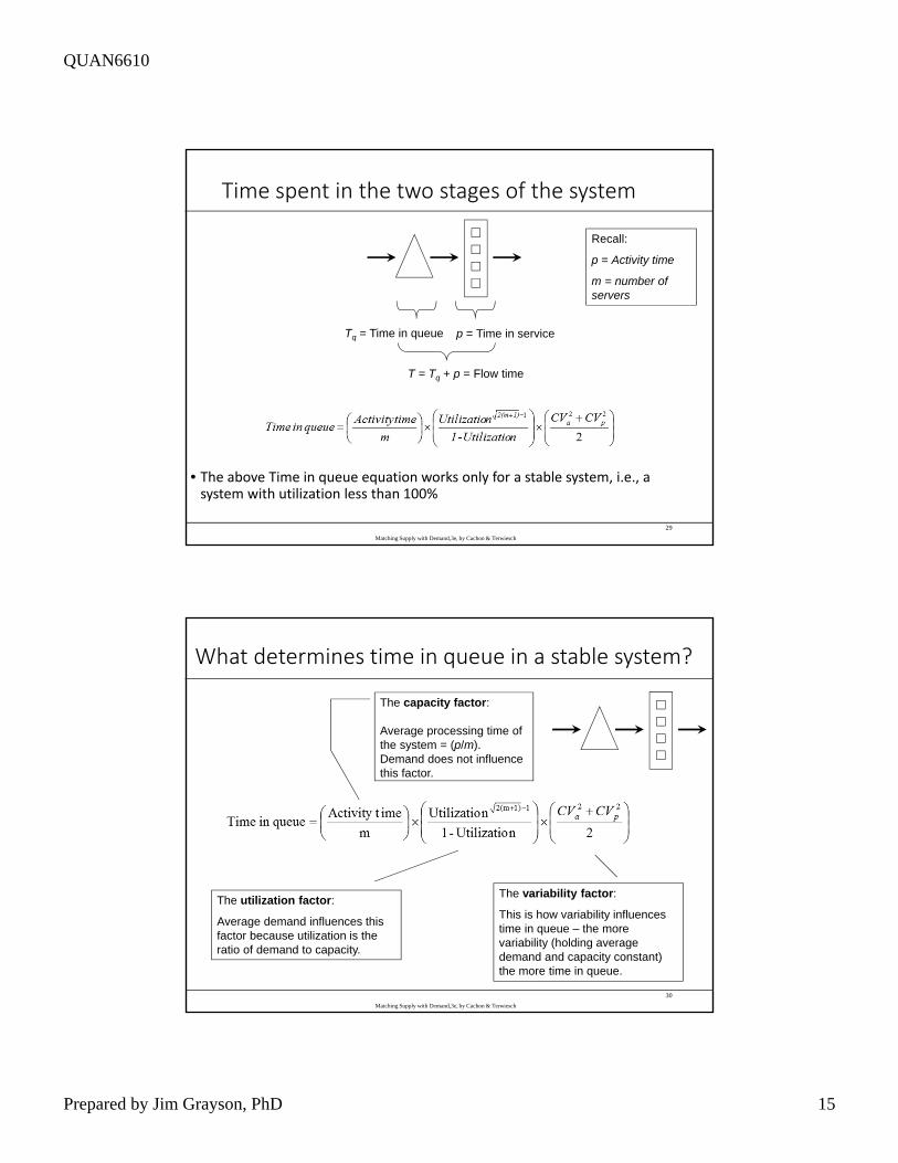
Time spent in the two stages of the system

• The above Time in queue equation works only for a stable system, i.e., a system with utilization less than 100%

Tq = Time in queue p = Time in service

T = Tq + p = Flow time

Recall:

p = Activity time

m = number of servers

29


What determines time in queue in a stable system?

The capacity factor:

Average processing time of the system = (p/m).Demand does not influence this factor.

The utilization factor:

Average demand influences this factor because utilization is the ratio of demand to capacity.

The variability factor:

This is how variability influences time in queue – the more variability (holding average demand and capacity constant) the more time in queue.

30


QUAN6610


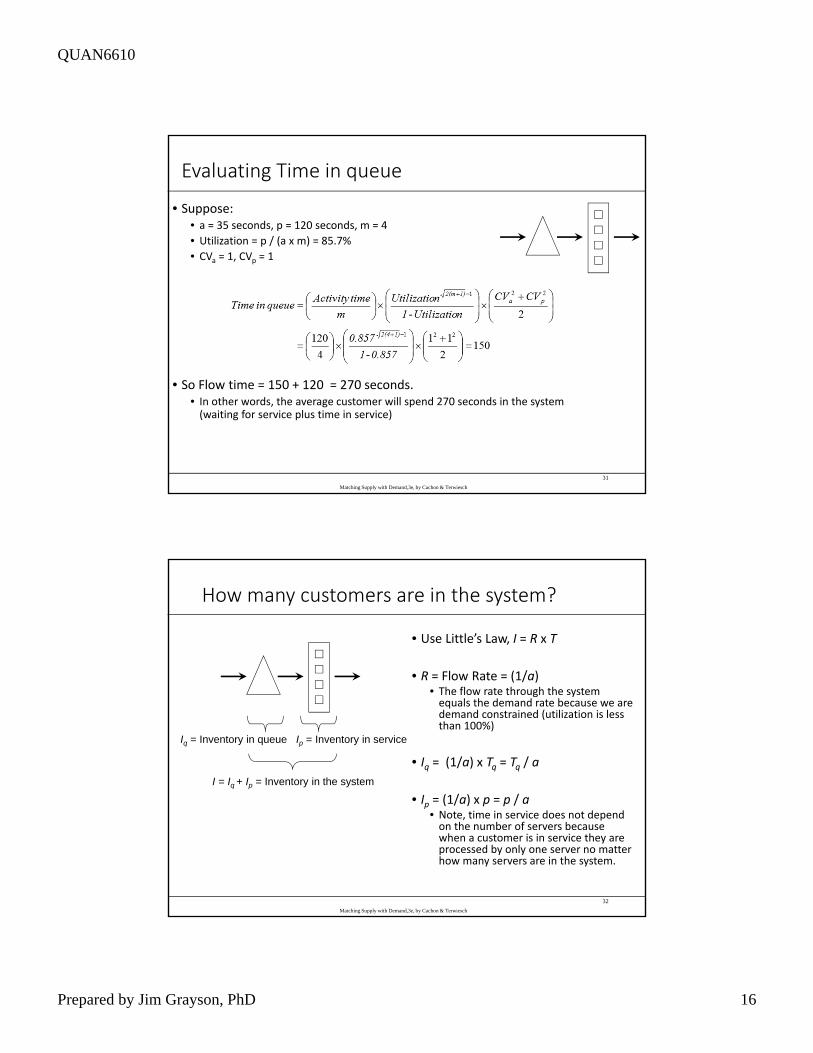
Evaluating Time in queue

• Suppose:• a = 35 seconds, p = 120 seconds, m = 4

• Utilization = p / (a x m) = 85.7%

• CVa = 1, CVp = 1

• So Flow time = 150 + 120 = 270 seconds.• In other words, the average customer will spend 270 seconds in the system (waiting for service plus time in service)

31


How many customers are in the system?

• Use Little’s Law, I = R x T

• R = Flow Rate = (1/a)• The flow rate through the system equals the demand rate because we are demand constrained (utilization is less than 100%)

• Iq = (1/a) x Tq = Tq / a

• Ip = (1/a) x p = p / a• Note, time in service does not depend on the number of servers because when a customer is in service they are processed by only one server no matter how many servers are in the system.

Iq = Inventory in queue Ip = Inventory in service

I = Iq + Ip = Inventory in the system

32


QUAN6610


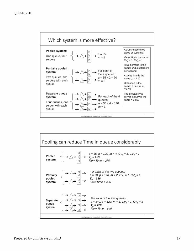
Which system is more effective?

Pooled system:

One queue, four servers

Partially pooled system:

Two queues, two servers with each queue.

Separate queue system:

Four queues, one server with each queue.

a = 35m = 4

For each of the 2 queues:a = 35 x 2 = 70m = 2

For each of the 4 queues:a = 35 x 4 = 140m = 1

Across these three types of systems:

Variability is the same: CVa = 1, CVp = 1

Total demand is the same: 1/35 customers per second.

Activity time is the same: p = 120

Utilization is the same: p / a x m = 85.7%

The probability a server is busy is the same = 0.857

33


Pooling can reduce Time in queue considerably

Pooled system

Partially pooled system

Separate queue system

a = 35, p = 120, m = 4, CVa = 1, CVp = 1Tq = 150Flow Time = 270

For each of the two queues:a = 70, p = 120, m = 2, CVa = 1, CVp = 1Tq = 336Flow Time = 456

For each of the four queues:a = 140, p = 120, m = 1, CVa = 1, CVp = 1Tq = 720Flow Time = 840

34


QUAN6610


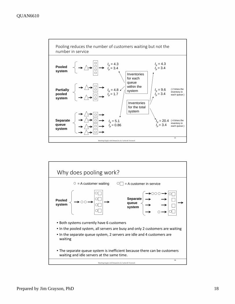
Pooling reduces the number of customers waiting but not the number in service

Pooled system

Partially pooled system


Iq = 4.3Ip = 3.4

Iq = 4.8Ip = 1.7

Iq = 5.1Ip = 0.86

Iq = 4.3Ip = 3.4

Iq = 9.6Ip = 3.4

Iq = 20.4Ip = 3.4

Inventories for each queue within the system

Inventories for the total system

( 2 times the inventory in each queue )

( 4 times the inventory in each queue )

35


Why does pooling work?

• Both systems currently have 6 customers

• In the pooled system, all servers are busy and only 2 customers are waiting

• In the separate queue system, 2 servers are idle and 4 customers are waiting

• The separate queue system is inefficient because there can be customers waiting and idle servers at the same time.

Pooled system


= A customer waiting = A customer in service

36


QUAN6610


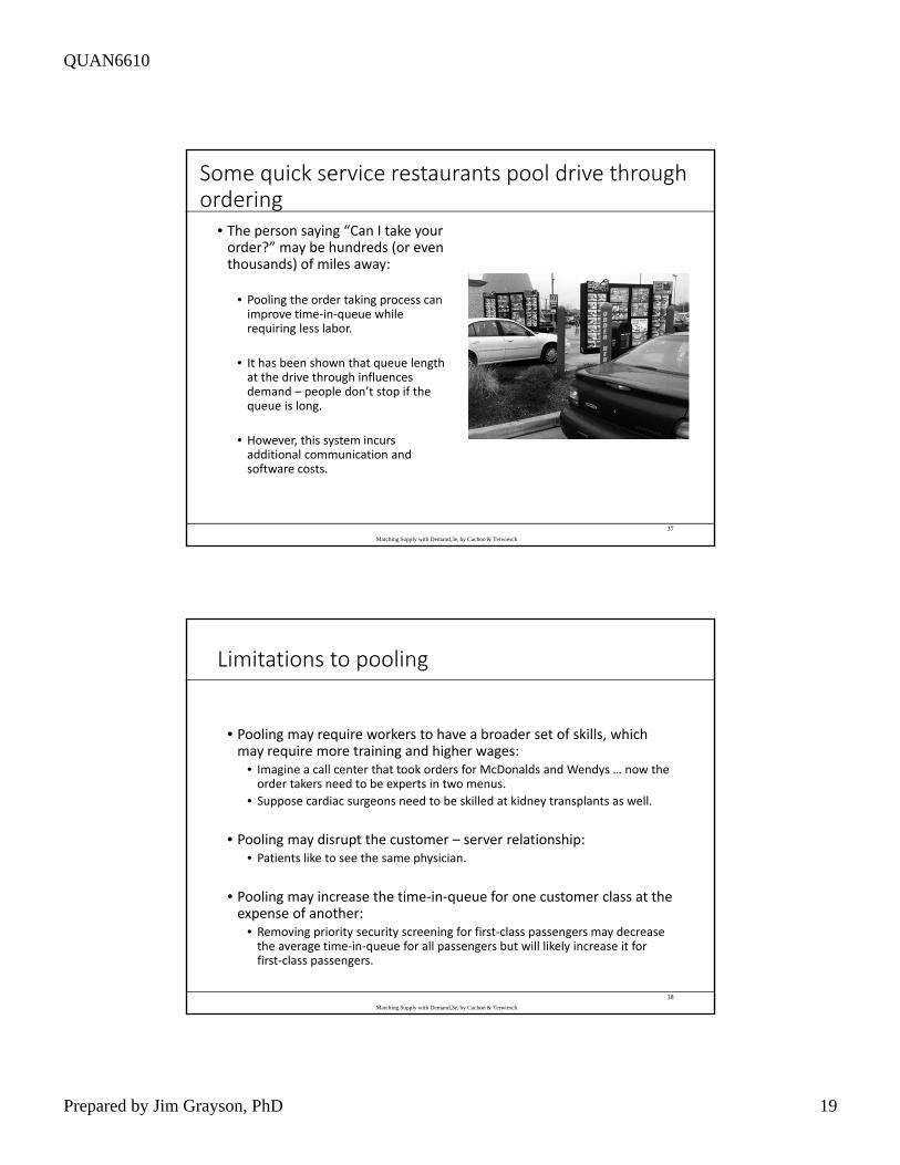
Some quick service restaurants pool drive through ordering

• The person saying “Can I take your order?” may be hundreds (or even thousands) of miles away:

• Pooling the order taking process can improve time‐in‐queue while requiring less labor.

• It has been shown that queue length at the drive through influences demand – people don’t stop if the queue is long.

• However, this system incurs additional communication and software costs.

37


Limitations to pooling

• Pooling may require workers to have a broader set of skills, which may require more training and higher wages:

• Imagine a call center that took orders for McDonalds and Wendys … now the order takers need to be experts in two menus.

• Suppose cardiac surgeons need to be skilled at kidney transplants as well.

• Pooling may disrupt the customer – server relationship:• Patients like to see the same physician.

• Pooling may increase the time‐in‐queue for one customer class at the expense of another:

• Removing priority security screening for first‐class passengers may decrease the average time‐in‐queue for all passengers but will likely increase it for first‐class passengers.

38


QUAN6610


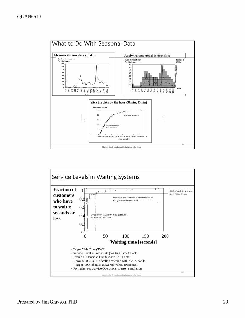
What to Do With Seasonal Data

Measure the true demand data

Slice the data by the hour (30min, 15min)

Apply waiting model in each slice

39


• Target Wait Time (TWT)• Service Level = Probability{Waiting TimeTWT}• Example: Deutsche Bundesbahn Call Center

- now (2003): 30% of calls answered within 20 seconds- target: 80% of calls answered within 20 seconds

• Formulas: see Service Operations course / simulation

0

0.2

0.4

0.6

0.8

1

0 50 100 150 200Waiting time [seconds]

Fraction of customers who have to wait xseconds or less

Waiting times for those customers who do not get served immediately

Fraction of customers who get served without waiting at all

90% of calls had to wait 25 seconds or less

Service Levels in Waiting Systems

40


QUAN6610


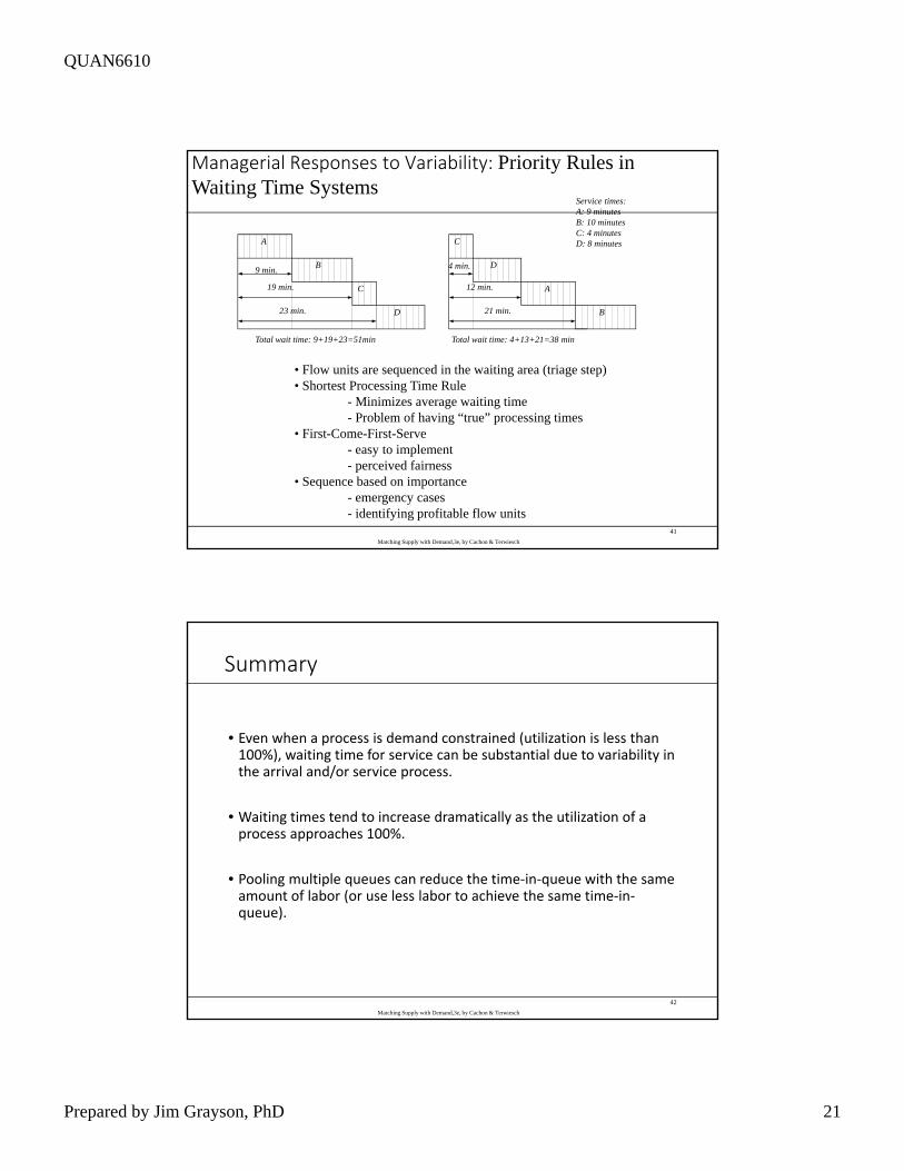
Service times:A: 9 minutesB: 10 minutesC: 4 minutesD: 8 minutes

D

A

C

B9 min.

19 min.

23 min.

Total wait time: 9+19+23=51min

B

D

A

C

4 min.

12 min.

21 min.

Total wait time: 4+13+21=38 min

• Flow units are sequenced in the waiting area (triage step)• Shortest Processing Time Rule

- Minimizes average waiting time- Problem of having “true” processing times

• First-Come-First-Serve- easy to implement- perceived fairness

• Sequence based on importance- emergency cases- identifying profitable flow units

Managerial Responses to Variability: Priority Rules in Waiting Time Systems

41


Summary

• Even when a process is demand constrained (utilization is less than 100%), waiting time for service can be substantial due to variability in the arrival and/or service process.

• Waiting times tend to increase dramatically as the utilization of a process approaches 100%.

• Pooling multiple queues can reduce the time‐in‐queue with the same amount of labor (or use less labor to achieve the same time‐in‐queue).

42


Documents

Variability –Waiting Times - Augusta Universityspots.gru.edu/jgrayson/MBAOpsMgt/CachonMSWDCurrentLectureSlides...QUAN6610 Prepared by Jim Grayson, PhD 1 Variability –Waiting Times