Variable Selection for Partially Linear Models With ...stefanski/mem_reports_2011/variable selection...Variable Selection for Partially Linear Models ... X, Z) ¼ 0, U is the measure-

Variable Selection for Partially Linear ModelsWith Measurement Errors

Hua LIANG and Runze LI

This article focuses on variable selection for partially linear models when the covariates are measured with additive errors. We propose two

classes of variable selection procedures, penalized least squares and penalized quantile regression, using the nonconvex penalized principle.

The first procedure corrects the bias in the loss function caused by the measurement error by applying the so-called correction-for-

attenuation approach, whereas the second procedure corrects the bias by using orthogonal regression. The sampling properties for the two

procedures are investigated. The rate of convergence and the asymptotic normality of the resulting estimates are established. We further

demonstrate that, with proper choices of the penalty functions and the regularization parameter, the resulting estimates perform asymp-

totically as well as an oracle property. Choice of smoothing parameters is also discussed. Finite sample performance of the proposed variable

selection procedures is assessed by Monte Carlo simulation studies. We further illustrate the proposed procedures by an application.

KEY WORDS: Errors-in-variable; Error-free; Error-prone; Local linear regression; Quantile regression; smoothly clipped absolute

deviation.

1. INTRODUCTION

Various linear and nonlinear parametric models have beenproposed for statistical modeling in the literature. However,these statistical parametric models and methods may not beflexible enough when dealing with real, high-dimensional data,which are frequently encountered in biological research. Avariety of semiparametric regression models have been pro-posed for a partial remedy to the ‘‘curse of dimensionality’’termed by Bellman (1961) to describe the exponential growthof volume as a function of dimensionality. In this article, wefocus on partially linear models, a class of commonlyused andstudied semiparametric regression models, which can retain theflexibility of nonparametric models and ease of interpretation oflinear regression models while avoiding the ‘‘curse of dimen-sionality.’’ Specifically, we shall propose variable selection pro-cedures for partially linear models when the linear covariates aremeasured with errors.

In practice, many explanatory variables are generally col-lected and need to be assessed during the initial analysis.Deciding which covariates to keep in the final statistical modeland which variables are noninformative is practically inter-esting, but is always a tricky task for data analysis. Variableselection is therefore of fundamental interest in statisticalmodeling and analysis of data, and has become an integral partin most of the widely used statistics packages. No doubt vari-able selection will continue to be an important basic strategyfor data analysis, particularly as high throughput technologiesbrings us larger datasets with a greater number of exploratoryvariables. The development of variable selection procedureshas progressed rapidly since the 1970s. Akaike (1973) pro-posed the Akaike information criterion (AIC). Hocking (1976)

gave a comprehensive review on the early developments ofvariable selection procedure for linear models. Schwarz (1978)developed the Bayesian information criterion (BIC), and Fosterand George (1994) developed the risk inflation criterion (RIC).With these criteria, stepwise regression or the best subsetselection are frequently used in practice, but these proceduressuffer from several drawbacks, such as the lack of stability asnoted by Breiman (1996) and lack of incorporating stochasticerrors inherited in the stage of variable selection. In an attemptto overcome these drawbacks, Fan and Li (2001) proposed aclass of variable selection procedures for parametric models viaa nonconcave-penalized-likelihood approach, which simulta-neously selects significant variables and estimates unknownregression coefficients. Starting with the seminal work byMitchell and Beauchamp (1988), Bayesian variable selectionhas become a very active research topic during the last twodecades. Pioneer work includes Mitchell and Beauchamp(1988), George and McCulloch (1993), and Berger and Perc-chi (1996). See Raftery, Madigan, and Hoeting (1997), Hoet-ing, Madigan, Raftery, and Volinsky (1999), and Jiang (2007)for more recent developments.

Some variable selection procedures for partially linearmodels include Bunea (2004) and Bunea and Wegkamp (2004),which developed model selection criteria for partially linearmodels with independent and identically distributed data.Bunea (2004) proposed a covariate selection procedure, whichestimates the parametric and nonparametric components simul-taneously, for partially linear models via penalized leastsquares with a L0 penalty. Bunea and Wegkamp (2004) pro-posed a two-stage model selection procedure that first esti-mates the nonparametric component, and then selects thesignificant variables in the parametric component. Their pro-cedure is similar to a one-step backfitting algorithm with agood initial estimate for the nonparametric component. Inaddition, Fan and Li (2004) proposed a profile least squaresapproach for partially linear models for longitudinal data.

Measurement error data are often encountered in manyfields, including engineering, economics, physics, biology,

Hua Liang is Professor, Department of Biostatistics and ComputationalBiology, University of Rochester, NY 14642 (E-mail: [email protected]). Runze Li is Professor, Department of Statistics and The MethodologyCenter, The Pennsylvania State University, University Park, PA 16802-2111(E-mail: [email protected]). Liang’s research was partially supported by NIH/-NIAID grants AI62247 and AI59773 and NSF grant DMS-0806097. Li’s researchwas supported by a National Institute on Drug Abuse (NIDA) grant P50DA10075 and NSF grant DMS-0348869. The authors thank the editor, anassociate editor, and two reviewers for their constructive comments and sug-gestions. They also thank John Dziak and Jeanne Holden-Wiltse for theireditorial assistance. The content is solely the responsibility of the authors anddoes not necessarily represent the official views of the NIDA or the NationalInstitutes of Health.

234

� 2009 American Statistical AssociationJournal of the American Statistical Association

March 2009, Vol. 104, No. 485, Theory and MethodsDOI 10.1198/jasa.2009.0127

biomedical sciences, and epidemiology. For example, inacquired immunodeficiency syndrome (AIDS) studies, viro-logic and immunologic markers, such as plasma concentrationsof human immunodeficiency virus (HIV)-1 RNA and CD4 þcell counts, are measured with errors. Statistical inferencemethods for various parametric measurement error modelshave been well established over the past several decades. Fuller(1987) and Carroll, Ruppert, Stefanski, and Crainiceanu (2006)gave a systematic survey on this research topic and presentedmany applications of measurement error data. Partially linearmodels have been used to study measurements with errors(Wang, Lin, Gutierrez, and Carroll 1998; Liang, Hardle, andCarroll 1999; Ma and Carroll 2006; Liang, Wang, and Carroll2007; Pan, Zeng, and Lin 2008).

To the best of our knowledge, most existing variable selec-tion procedures are limited to directly observed predictors.Variable selection for measurement error data imposes chal-lenges for statisticians. For linear regression models containingmore than two covariates, some of which are measured witherror and others are error-free, it can be shown that the ordinaryleast squares method, which directly substitutes the observedsurrogates for the unobserved error-prone variables, yields aninconsistent estimate for the regression coefficients, becausethe loss function contains the error-prone covariates and theexpected value of the corresponding estimating function doesnot equal zero. The inconsistency nullifies the theoreticalproperty of the ordinary penalized least squares estimatewithout accounting for the measurement error. Note that mostvariable selection procedures are equivalent or asymptoticallyequivalent to minimizing a penalized least squares function.Thus, in the presence of measurement error, the existingpenalized least squares variable selection procedures ignoringmeasurement errors may not work properly. Extension of theexisting methods of variable selection accounting for meas-urement error is therefore by no means straightforward. Thus,we are motivated to develop variable selection procedures formeasurement error data. The proposed procedures resultmodels with a parsimonious and well-fitting subset of observedcovariates. We will consider the situation in which the cova-riates are measured with additive errors. Hence, selection ofobserved covariates with measurement error is equivalent toselection of the corresponding latent covariates. The coef-ficients of the observed surrogates and the associated latentcovariates have the same meaning.

In this article, we propose two classes of variable selectionprocedures for partially linear measurement error models: onebased on penalized least squares, and the other based onpenalized quantile regression. The former is more familiar andcomputationally easier, whereas the latter is more robust tooutliers. Our proposed strategy to correct the estimation biasdue to measurement error for the penalized least squares isquite different from that for the penalized quantile regression.For the penalized least squares method, we correct the bias bysubtracting a bias correction term from the least squaresfunction. For the penalized quantile regression, we correct thebias by using orthogonal regression (Cheng and Van Ness1999). To investigate the sample properties of the proposedprocedures, we first demonstrate how the rate of convergenceof the resulting estimates depends on the tuning parameter in

the penalized models. With proper choice of the penaltyfunction and the tuning parameter, we show that the resultingestimates of the proposed procedures asymptotically performas well as an oracle procedure, in the terminology of Fan and Li(2001). Practical implementation issues, including smoothingparameter selection and tuning parameter selection, areaddressed. We conduct Monte Carlo simulation experiments toexamine the performance of the proposed procedures withmoderate sample sizes, and compare the performance of theproposed penalized least squares and penalized quantileregression with various penalties. We also compare the per-formance of the proposed procedures with naive extension ofthe best subset variable selection from the ordinary linearregression models. Our simulation results demonstrate that theproposed procedures perform with moderate sample sizesalmost as well as the oracle estimator.

The rest of this article is organized as follows. In Section 2,we propose a class of variable selection procedures for partiallylinear measurement error models via penalized least squares. InSection 3, we develop a penalized quantile regression proce-dure for selecting significant variables in the partially linearmeasurement error models when considering the effects ofoutliers. Simulation results are presented in Section 4, and wealso illustrate the proposed procedures by an empirical analysisof a real dataset. Regularity conditions and technical proofs aregiven in the Appendix.

2. PENALIZED LEAST SQUARED METHOD

Suppose that {(Wi, Zi, Yi), i ¼ 1, . . ., n} is a random samplefrom the partially linear measurement error model (PLMeM),

Y ¼ XTbþ nðZÞ þ e;W ¼ Xþ U;

�ð1Þ

where Z is a univariate observed error-free covariate, X is ad-dimensional vector of unobserved latent covariates, which ismeasured in an error-prone way, W is the observed surrogate ofX, e is the model error with E(e |X, Z) ¼ 0, U is the measure-ment error with mean zero and (possibly singular) covariancematrix Suu. Thus, X may consist of some error-free variables.In this section, it is assumed that U is independent of (X, Z, Y).For example, Z could be measurement time, X could be avector of biomarkers like T-cell count or blood pressure, Wcould be the measured values for the quantities X, and U is thedifference between the observed W and unknown X. In thisarticle, we only consider univariate Z. The proposed method isapplicable for multivariate Z. The extension to the multivariateZ might be practically less useful due to the ‘‘curse of dimen-sionality.’’

To get insights into the penalized least squares procedure, wefirst consider the situation in which Suu is known. We willstudy the case of unknown Suu later on. Define a least squaresfunction to be

1

2

Xn

i¼1

fYi �WTi b� nðZiÞg2 � n

2bTSuub:

The second term is included to correct the bias in the squaredloss function due to measurement error. Since E(U|Z) ¼ 0,

Liang and Li: Variable Selection for Measurement Error Data 235

n(Z)¼ E(Y|Z)� E(W|Z)Tb. Then the least squares function canbe rewritten as

1

2

Xn

i¼1

½fYi � EðYijZiÞg � fWi � EðWijZiÞgTb�2 � n

2bTSuub:

This motivates us to consider a penalized least squares methodbased on partial residuals. Denote mw(Z)¼ E(W|Z) and my(Z)¼E(Y|Z). Let bmwð�Þ and bmyð�Þ be estimates of mw(�) and my(�),respectively. In this article, we employ local linear regression(Fan and Gijbels 1996) to estimate both mw(�) and my(�). Thebandwidth selection for the local linear regression is discussedin Section 4.1. The penalized least squares function based onpartial residuals is defined as

LPðSuu;bÞ ¼1

2

Xn

i¼1

½fYi � bmyðZiÞg � fWi � bmwðZiÞgTb�2

� n

2bTSuubþ n

Xd

j¼1

pljnðjbjjÞ;

where pljnð�Þ is a penalty function with a tuning parameter ljn,

which may be chosen by a data-driven method. For the sake ofsimplicity of notation, we use lj to stand for ljn throughout thisarticle. We will discuss the selection of the tuning parameter inSection 4.1. Denote bYi ¼ Yi � bmyðZiÞ andcWi ¼Wi � bmwðZiÞ:Thus, LP (Suu, b) can be written as

L PðSuu;bÞ ¼1

2

Xn

i¼1

ðbYi �cW Ti bÞ2 � n

2bTSuub

þ nXd

j¼1

pljðjbjjÞ: ð2Þ

Minimizing LP (Suu, b) with respect to b results in a penalizedleast squares estimator bb: It is worth noting that the penaltyfunctions and the tuning parameters are not necessarily thesame for all coefficients. For instance, we want to keepimportant variables in the final model, and therefore we shouldnot penalize their coefficients.

The penalized least squares function (2) provides a generalframework of variable selection for PLMeM. Taking the pen-alty function to be the L0-penalty (also called the entropypenalty in the literature), namely, plj

ðjbjjÞ ¼ 0:5l2j Ifjbjj 6¼ 0g;

where I{�} is an indicator function, we may extend the tradi-tional variable selection criteria, including the AIC (Akaike1973), BIC (Schwarz 1978), and RIC (Foster and George1994), for the PLMeM:

1

2

Xn

i¼1

ðbYi �cW Ti bÞ2 � n

2bTSuubþ n

2

Xd

j¼1

l2j Ifjbjj 6¼ 0g ð3Þ

asPd

j¼1 Ifjbjj 6¼ 0g equals the size of the selected model.Specifically, the AIC, BIC, and RIC correspond to lj[s

ffiffiffiffiffiffiffiffi2=n

p;

sffiffiffiffiffiffiffiffiffiffiffiffiffiffiffiffiffiffilogðnÞ=n

p; and s

ffiffiffiffiffiffiffiffiffiffiffiffiffiffiffiffiffiffilogðdÞ=n

p; respectively.

Note that the L0-penalty is discontinuous and thereforeoptimizing (3) requires exhaustive search over 2d possiblesubsets. This search poses great computational challenges.Furthermore, as noted by Breiman (1996), the best subsetvariable selection suffers from several drawbacks, including itslack of stability. In the recent literature of variable selection forlinear regression model without measurement error, many

authors advocated the use of continuous and smooth penaltyfunctions, for example, Bridge regression (Frank and Friedman1993) corresponding to the Lq-penalty pl(|bj|) ¼ q�1l|bj|

q; theleast absolute shrinkage and selection operator (LASSO)(Tibshirani 1996) corresponding to the L1-penalty. Fan and Li(2001) studied the choice of penalty functions in depth. Theyadvocated the use of the smoothly clipped absolute deviation(SCAD) penalty, defined by

plðjbjÞ ¼ljbj; if0 # jbj < l;ða2�1Þl2�ðjbj�alÞ2

2ða�1Þ ; if l # jbj< al;ðaþ1Þl2

2 ; if jbj $ al;

8><>:where a ¼ 3.7. For simplicity of presentation, we will use thename ‘‘SCAD’’ for all procedures using the SCAD penalty. Asdemonstrated in Fan and Li (2001), the SCAD is an improve-ment of the LASSO in terms of modeling bias and of the bridgeregression with q < 1 in terms of stability.

We next study the sampling property of the resulting penalizedleast squares estimate. Let b0 ¼ ðb10; . . .;bd0ÞT ¼ ðbT

10;bT20Þ

T

be the true value of b. Without loss of generality, assume that b10

consists of all nonzero components of b0, and b20 ¼ 0. Let sdenote the dimension of b10. Denote

an ¼ max1 # j # d

fjp0ljðjbj0jÞj;bj0 6¼ 0g; and bn

¼ max1 # j # d

fjp00ljðjbj0jÞj;bj0 6¼ 0g; ð4Þ

b ¼ fp0l1ðjb10jÞsgnðb10Þ; . . .; p0ls

ðjbs0jÞsgnðbs0ÞgT;

and Sl ¼ diagfp00l1ðjb10jÞ; . . .; p00ls

ðjbs0jÞg:ð5Þ

In what follows, A52 ¼ AAT for any vector or matrix A. Let~§ ¼ §� Eð§jZÞ for any random variable/vector §. For example,eX ¼ X� EðXjZÞ: Denote by S*1 the elements of S* withrespect to b10 for any random/function vector S*. For example,U11 and eX11 are the vectors included by the first s elements ofU1 and eX1; respectively. Let Suu1 be the (s, s) � left uppersubmatrix of Suu, and SX|Z ¼ cov{X11 � E(X11|Z1)}. ||v||denotes the Euclidean norm for the vector v. We have thefollowing theorem, whose proof is given in the Appendix.

Theorem 1. Suppose that an ¼ O(n�1/2), bn ! 0, and theregularity conditions (a)–(e) in the Appendix hold. Then wehave the following conclusions.

(1) With probability approaching one, there exists a localminimizer b of LPðSuu;bÞ such that k b� b k¼Opðn�1=2Þ:

(2) Further assume that all lj! 0, n1/2 lj ! ‘, and

lim infn!‘

flim infu!0þ

p0ljðuÞ=ljg > 0: ð6Þ

With probability approaching one, the root n consistentestimator b in (1) satisfies (a) b2 ¼ 0; and (b) b1 has anasymptotic normal distributionffiffiffi

npðSXjZ þ SlÞfbb1 � b10 þ ðSXjZ þ SlÞ�1bg !D Nð0;GÞ;

whereG ¼ E eX11ðe� UT

11b10Þ þ eU11 þ ðU11UT11 � Suu1Þb10

n o�2

:

236 Journal of the American Statistical Association, March 2009

To make statistical inference on b10, we need to estimate thestandard error of the estimator bb1: From Theorem 1, theasymptotic covariance matrix of bb1 is

1

nðSXjZ þ SlÞ�1

GðSXjZ þ SlÞ�1:

A consistent estimate of SX|Z is defined as

ðn� sÞ�1Xn

i¼1

cW�2i1 � Suu1 ¼

def bSXjZ:

Furthermore, G can be estimated by

bGn ¼ n�1Xn

i¼1

cWi1ðbYi �cWTi1bb1Þ þ Suu1

bb1

n o�2

:

The covariance matrix of the estimates bb1; the nonvanishingcomponent of bb1; can be estimated by

n�1 bSXjZ þ Slðbb1Þn o�1bGn

bSXjZ þ Slðbb1Þn o�1

; ð7Þ

where Slðbb1Þ is obtained by replacing b1 by bb1 in Sl.

Remark 1. The proposed penalized least squares proce-dure can directly be applied for a linear measurement errormodel, which can be regarded as a PLMeM in the absence ofthe nonparametric component n(Z). Thus, under the conditionsof Theorem 1, the resulting estimate obtained from the penal-ized least squares function (3) is

ffiffiffinp

consistent, and satisfiesb2 ¼ 0; andffiffiffi

npfcovðX11Þ þ Slgbb1 � b10 þ fcovðX11Þ þ Slg�1b

h i!D N 0;G0ð Þ;

whereG0 ¼ E X11ðe� UT

11b10Þ þ eU11 þ ðU11UT11 � Suu1Þb10

� ��2:

We now consider the situation in which Suu is unknown. Toestimate Suu, it is common to assume that there are partiallyreplicated observations, so that we observe Wij ¼ Xi þ Uij forj ¼ 1, . . ., Ji (Carroll, et al. 2006, chap. 3). Let Wi ¼J�1

i

PJi

j¼1 Wij be the sample mean of the replicates. Then aconsistent, unbiased method of moments estimate for Suu is

bSuu ¼Xn

i¼1

XJi

j¼1

ðWij �WiÞ�2=Xn

i¼1

ðJi � 1Þ:

Let Ui ¼ J�1i

PJi

j¼1 Uij: Note that covðUiÞ ¼ J�1i Suu: Thus, the

penalized least squares function is defined as

L PðbSuu;bÞ ¼1

2

Xn

i¼1

fðbYi �cWT

i bÞ2 � J�1i bTbSuubg

þ nXd

j¼1

pljðjbjjÞ; ð8Þ

wherecWi ¼Wi � mwðZiÞ and mwðzÞ is local linear estimate ofEðWijZi ¼ zÞ: Throughout this section, we assume that1=n

Pni¼1 J�1

i converges to a finite constant as n ! ‘.

Theorem 2. Under the conditions of Theorem 1, we stillhave the following conclusions:

(1) With probability approaching one, there exists a local

minimizer b of LPðbSuu;bÞ defined in (8) such thatk b� b k¼ Opðn�1=2Þ:(2) Further assume that all lj! 0,

ffiffiffinp

lj ! ‘; and (6) holds.With probability approaching one, the root n consistentestimate b in (1) satisfies b2 ¼ 0; andffiffiffi

npðSXjZ þ SlÞfbb1 � b10 þ ðSXjZ þ SlÞ�1bg!D Nð0;G�Þ;

where G� ¼ limn!‘

1n

Pni¼1 Ef ~Xi1ðei � U

T

i1b10Þ þ eiUi1

þðUi1UT

i1 � J�1i Suu1Þb10g�2: and Ui1 is the average of

{Uij1, j ¼ 1, . . ., ji}.

As a special case, if Ji [ J0 > 1, then it follows

G�¼ E eX11ðe� UT

11b10Þ þ eU11 þ ðU11UT

11 � J�10 Suu1Þb10

n o�2

:

Because bSuu is a consistent, unbiased estimator of Suu,Theorem 2 can be proved in a similar way to Theorem 1 byreplacing LPðSuu;bÞ by LPðbSuu;bÞ: To save space, we omitthe details.

We next derive an estimate of the standard error of b1: Aconsistent estimator of SX|Z is defined as

ðn� sÞ�1Xn

i¼1

Wi1 � bEðWi1jZiÞn o�2

� 1

Ji

bSuu1

� �;

where bSuu1 is the (s, s)—left upper submatrix of bSuu: Estimatesof G* can be also easily obtained. Let

Ri ¼cWi1ðbYi �cW T

i1bb1Þ þ bSuu1

bb1

.J

i:

Then a consistent estimate of G* is the sample covariancematrix of the Ri’s. See Liang, et al. (1999) for a detailed dis-cussion.

3. PENALIZED QUANTILE REGRESSION

In the presence of outliers, the least squares method mayperform badly. Quantile regression is taken as a useful alter-native and has been popular in both the statistical and econo-metric literature. Koenker (2005) provided a comprehensivereview on quantile regression techniques. In this section, weexplore robust variable selection, and propose a class ofpenalized quantile-regression variable selection procedures forPLMeM in the presence of contaminated response observa-tions.

In the penalized least squares procedure discussed in theprevious section, the term �nbTSuub was included in the lossfunction (2) to correct the estimation bias due to measurementerror of the ordinary least squares estimate. However, thisapproach cannot be extended to quantile regression for cor-recting the estimation bias because a direct subtraction cannotcorrect the bias. We now propose a penalized quantile functionbased on the orthogonal regression. That is, the objectivefunction is defined as the sum of squares of the orthogonaldistances from the data points to the straight line of regressionfunction, instead of the residuals obtained from the classicalregression (Cheng and Van Ness 1999). The orthogonalregression has been used to correct estimation bias due to


measurement error of the least squares estimate of regressioncoefficients in linear measurement error models (Lindley 1947;Madansky 1959). He and Liang (2000) applied the idea oforthogonal regression for quantile regression for both linearmodels and partially linear models with measurement errors.However, they did not consider variable selection problems.Partly motivated by the work of He and Liang (2000), wefurther used the orthogonal regression method to develop apenalized quantile regression procedure to select significantvariables in the partially linear models.

To define orthogonal regression for quantile regression withmeasurement error data, it is assumed that the random vector (e,UT) follows an elliptical distribution with mean zero and cova-riance matrix s2S, where s2 is unknown, whereas S is a blockdiagonal matrix with (1,1)-element being 1 and the last d 3 ddiagonal block matrix being Cuu. Readers are referred to Fang,Kotz, and Ng (1990) for details about elliptical distributions andLi, et al. (1997) for tests of spherical and elliptical symmetry.The matrix Cuu is proportional to Suu and is assumed to beknown in this section. As discussed in the last section, it can beestimated with partially replicated observations in practice.

Denote rt the tth quantile objective function,

rtðrÞ ¼ t maxðr; 0Þ þ ð1� tÞmaxð�r; 0Þ: ð9ÞNote that the solution to minimizing Ert(e � u) over u 2 R isthe tth quantile of e. Define penalized quantile function to be ofthe form:

LtðbÞ ¼defXn

i¼1

rt

bYi �cWTi bffiffiffiffiffiffiffiffiffiffiffiffiffiffiffiffiffiffiffiffiffiffiffiffi

1þ bTCuubp !

þ nXd

j¼1

pljðjbjjÞ: ð10Þ

He and Liang (2000) proposed the quantile regression estimatefor b by minimizing the first term in (10). However, it wasassumed in He and Liang (2000) that (e, UT) follows a sphericaldistribution (i.e., Cuu ¼ Id). The sphericity assumption impliesthat the elements of U are uncorrelated. Here, we relax thesphericity assumption. He and Liang (2000) also providedinsights into why to use the first term in (10). Because ei andðei � UT

i bÞ=ffiffiffiffiffiffiffiffiffiffiffiffiffiffiffiffiffiffiffiffiffiffiffiffi1þ bTCuub

phave the same distribution on the

basis of the fact given in (A.8) in Section A.2, we can establishthe consistency for the resulting estimate by using similararguments to those in He and Liang (2000). Compared with thepenalized least squares function in (3), the penalized quantilefunction uses the factor

ffiffiffiffiffiffiffiffiffiffiffiffiffiffiffiffiffiffiffiffiffiffiffiffi1þ bTCuub

pto correct the bias in the

quantile loss function due to the presence of the error-pronevariables.

Let f(�) be the density function of e, an¼O(n�1/2), and bn! 0.

Theorem 3. Suppose that (ei, Ui) follows an ellipticaldistribution with mean zero and the covariance structureaforementioned for i ¼ 1, . . ., n. Assume that the equationErt(ei� q)¼ 0 has the unique solution, which is denoted by qt,and that f(v þ qt) � f(qt) ¼ O(v1/2) as v ! 0. Then,

(1) With probability tending to one, there exists a localminimizer bt of Lt(b) defined in (10) such that its rate ofconvergence is Op(n�1/2).(2) Further assume (6) holds. If all lj! 0,

ffiffiffinp

lj ! ‘; thenwith probability tending to one, the root n consistent esti-

mator bt ¼ ðbT

t1; bT

t2ÞT in (1) must satisfy (a) bt2 ¼ 0; and

(b)ffiffiffinp

f ðqtÞð1þ bT10C11b10Þ1=2

SXjZðbt1 � b10Þ þ nbð1þbT

10C11b10Þ1=2!D Nð0; JqÞ; where C11 is the first s 3 sdiagonal submatrix of Cuu, and

Jq ¼ tð1� tÞSXjZ

þ cov ctðjÞ U11 þjb10ffiffiffiffiffiffiffiffiffiffiffiffiffiffiffiffiffiffiffiffiffiffiffiffiffiffiffiffiffi

1þ bT10C11b10

q0B@

1CA8><>:

9>=>; ð11Þ

with j ¼ ðe� UT11b10Þ=

ffiffiffiffiffiffiffiffiffiffiffiffiffiffiffiffiffiffiffiffiffiffiffiffiffiffiffiffiffi1þ bT

10C11b10

q� qt and ct

being the derivative of rt. It is worth pointing out thatwhen Cuu ¼ Id and b ¼ 0, which corresponds to nopenalty term in (10), the asymptotic normality is the sameas that in He and Liang (2000). However, the conditionsimposed in Theorem 3 are weaker than those in He andLiang (2000).

4. SIMULATION STUDY AND APPLICATION

We now investigate the finite sample performance of theproposed procedures by Monte Carlo simulation, and illustratethe proposed methodology by an analysis of a real dataset. Inour numerical examples, we use local linear regression toestimate mw(z) and my(z) with the kernel function K(u) ¼0.75(1 � u2)I(|u| # 1).

4.1 Issues Related to Practical Implementation

In this section, we address practical implementation issues ofthe proposed procedures.

Bandwidth selection. Condition (b) in the Appendix requiresthat the bandwidths in estimating mw(�) and my(�) are of ordern–1/5. Any bandwidths with this rate lead to the same limitingdistribution for b: Therefore, the bandwidth selection can bedone in a standard routine. In our implementation, we use theplug-in bandwidth selector proposed in Ruppert, Sheather, andWand (1995) to select bandwidths for the estimation of mw(�)and my(�). In our empirical study, we have experimented withshifting bandwidths around the selected values, and found thatthe results are stable.

Local quadratic approximation. Because the penalty func-tions such as the SCAD penalty and the Lq penalty with 0 < q # 1are singular at the origin, it is challenging to minimize thepenalized least squares or quantile loss functions. Hunter andLi (2005) proposed a perturbed version of the local quadraticapproximation of Fan and Li (2001); i.e.,

pljðjbjjÞ � plj

ðjbð0Þj jÞ þ1

2fp0ljðjbð0Þj jÞ=ðjb

ð0Þj j þ hÞgðb2

j

� bð0Þ2j Þ ¼

defqljðjbjjÞ;

where h is a small positive number. Hunter and Li (2005) dis-cussed how to determine the value of h in detail. In our imple-mentation, we adopt their strategy to choose h. With the aid of theperturbed local quadratic approximation, the Newton–Raphsonalgorithm can be applied to minimize the penalized leastsquares or quantile loss function. We set the unpenalizedestimate bbu as the initial value of b.

Choice of regularization parameters. Here, we describe theregularization parameter selection procedure for the penalizedleast square function in (8) in detail. The idea can be directly


applied for the penalized least square function in (2) and thepenalized quantile regression. For the penalized least squaresfunction in (8), let

‘ðbÞ ¼1

2

Xn

i¼1

fYi � bmyðZiÞ � ðWi � bm�wðZÞÞTbg2 � J�1i bTbSuub

h i:

Then

LPðbSuu;bÞ ¼ ‘ðbÞ þ nXd

j¼1

qljðjbjjÞ:

Following Fan and Li (2001), we define the effective number ofparameters

eðlÞ ¼ tr½fL00PðbSuu; bÞg�1‘‘0ðbÞ�;where l ¼ (l1, . . ., ld), and, for any function g(b),g00ðbÞ ¼ @2gðbÞ

�@b@bT; the Hessian matrix of g(b). Fol-

lowing Wang, Li, and Tsai (2007), we define the BIC score tobe

BICðlÞ ¼ log RSSl þ eðlÞ � logðnÞ=n;

where RSSl is the residual sum of squares corresponding to themodel selected by the penalized least squares with the tuningparameters l. Minimizing BIC(l) with respect to l over a d-dimensional space is difficult. Fan and Li (2004) advocated thatthe magnitude of lj should be proportional to the standard errorof the unpenalized least squares estimator of bj, denoted by bbu

j :Following Fan and Li (2004), we take lj ¼ l � SEðbbu

j Þ; whereSE ðbbu

j Þis the estimated standard error of bbuj : Such a choice of

lj works well from our simulation experience. Thus, the min-imization problem over l will reduce to a one-dimensionalminimization problem, and the tuning parameter l, and theminimum can be obtained by a grid search. In our simulation,the range of l is selected to be wide enough so that the BICscore reaches its minimum approximately in the middle of therange, and 50 grid points are set to be evenly distributed overthe range of l.

For the penalized quantile regression, rt(�) is not differ-entiable at the origin. We use the MM algorithm proposed byHunter and Lange (2000) to minimize the penalized quantilefunction. In other words, we approximate rt(�) by a localquadratic function at each step during the course of iteration.This idea is similar to that of the perturbed local quadraticapproximation algorithm.

4.2 Simulation Studies

In our simulation study, we will compare the underlyingprocedures with respect to estimation accuracy and modelcomplexity for the penalized least squares and the penalizedquantile regression procedures. It is worth noting that the bestmethod for achieving the most accurate estimate (i.e., mini-mizing the squared error in Examples 1 and 2) need not coin-cide with the best method for having the sparsest model (i.e.,maximizing the expected number ‘‘C’’ of correctly deletedvariables and minimizing the expected number ‘‘I’’ of incor-rectly deleted variables in Examples 1 and 2).

Example 1. In this example we simulate 1,000 datasets,each consisting of n¼ 100, 200 random samples from PLMeM(1), in which n(z) ¼ 2 sin(2pz3). The covariates and randomerror are generated as follows. The covariate vector X is gen-erated from a 12-dimensional normal distribution with mean 0and variance 1. To study the effect of correlation amongcovariates on the performance of variable selection procedures,the off-diagonal elements of covariance matrix of X are set tobe cov(Xi, Xj)¼ 0.2 for i¼ 1, 2 and j¼ 1, . . ., 12, cov(Xi, Xj)¼0.5 for i, j ¼ 3, . . ., 6, cov(Xi, Xj) ¼ 0.8 for i, j ¼ 7, . . ., 10, andcov(Xi, Xj) ¼ 0.95 for i, j ¼ 11, 12. Thus, X1 and X2 are weaklycorrelated with the other X-variables, X3, . . ., X6 are moderatelycorrelated, while X7, . . ., X10 are strongly correlated. X11 andX12 are nearly collinear. In this example, we set b0 ¼ c1(1.5, 0,0.75, 0, 0, 0, 1.25, 0, 0, 0,1, 0)T with c1 ¼ 0.5, 1, and 2 so thatone of weakly, moderately, strongly correlated, or nearly col-linear covariates has nonzero coefficient, and the other cova-riates have zero coefficients. The covariate Z ¼ FfðX1þffiffiffi

3p

Z0Þ=2g; where Z0 ; N(0, 1) and F(�) is the cumulativedistribution of the standard normal distribution. Thus, Z ;

uniform(0, 1), but is correlated with the X-variables. Thecorrelation between Z and X1 is about 0.5, while the corre-lation between Z and Xj (j ¼ 2, . . ., 12) is about 0.1. In thisexample, we consider two scenarios to generate the randomerror: (a) e follows N(0, 1) (i.e., homogeneous error); and (b)e follows j sinf2pðXTbÞ2 þ 0:2ZgjðX2

2 � 2Þ; where X22

denotes the chi-squared distribution with 2 degrees of free-dom. This case is designed to investigate the effect ofasymmetric and heteroscedastic error on the estimators. Thefirst 2 components of X are measured with errors Uj, whichfollow a normal distribution with mean 0, variance c20.52,and correlation between U1 and U2 being 0.5. The last 10components of X are error free. To estimate Suu, two repli-cates of W are generated (i.e., Ji [ 2). To study the effect ofthe level of measurement error, we take c2 ¼ 1 and 2. A directcalculation indicates that the naive estimator of b will beconsistent to c1(1.12, � 0.10, 0.77, 0.02, 0.02, 0.02, 1.26,0.01, 0.02, 0.02, 1.04, 0.01) for c2 ¼ 1 and c1(0.91, � 0.13,0.78, 0.03, 0.04, 0.03, 1.26, 0.02, 0.02, 0.03, 1.06, 0.01) for c2

¼ 2. The magnitude of all elements, but the second of thesetwo vectors is the same as that of the corresponding elementsof b. This point was justified by Gleser (1992, pp. 690, 1992)that separate reliability studies of each component of Xgenerally cannot substitute for reliability studies of the vectorX treated as a unit. We therefore anticipate that if one ignoresmeasurement errors, any appropriate variable selection pro-cedures may falsely classify the second element of X as asignificant one. Consequently, the number of zero coef-ficients decreases to 7 from 8. Our simulation results laterexactly demonstrate this point, and further indicate thatignoring measurement error may cause errors in variableselection procedures. To save space, we present results forn ¼ 200 only. The results for other values of n are referred toLiang and Li (2008).

We first compare estimation accuracy for the penalized leastsquares procedures with and without considering measurementerrors. Table 1 depicts the median of squared error (MedSE),k b� b0 k2, over the 1,000 simulations. In Table 1, the toppanel is the MedSE of the penalized least squares procedures,


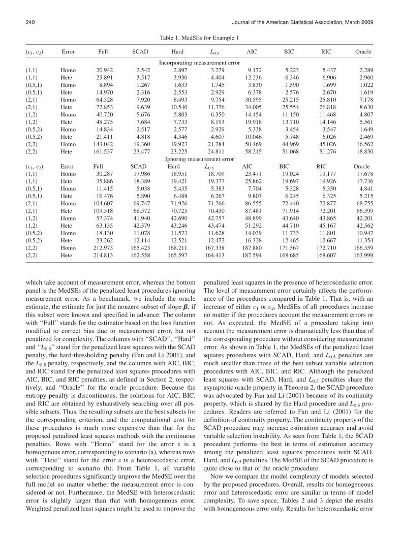
which take account of measurement error, whereas the bottompanel is the MedSEs of the penalized least procedures ignoringmeasurement error. As a benchmark, we include the oracleestimate, the estimate for just the nonzero subset of slope b, ifthis subset were known and specified in advance. The columnwith ‘‘Full’’ stands for the estimator based on the loss functionmodified to correct bias due to measurement error, but notpenalized for complexity. The columns with ‘‘SCAD’’, ‘‘Hard’’and ‘‘L0.5’’ stand for the penalized least squares with the SCADpenalty, the hard-thresholding penalty (Fan and Li 2001), andthe L0.5 penalty, respectively, and the columns with AIC, BIC,and RIC stand for the penalized least squares procedures withAIC, BIC, and RIC penalties, as defined in Section 2, respec-tively, and ‘‘Oracle’’ for the oracle procedure. Because theentropy penalty is discontinuous, the solutions for AIC, BIC,and RIC are obtained by exhaustively searching over all pos-sible subsets. Thus, the resulting subsets are the best subsets forthe corresponding criterion, and the computational cost forthese procedures is much more expensive than that for theproposed penalized least squares methods with the continuouspenalties. Rows with ‘‘Homo’’ stand for the error e is ahomogenous error, corresponding to scenario (a), whereas rowswith ‘‘Hete’’ stand for the error e is a heteroscedastic error,corresponding to scenario (b). From Table 1, all variableselection procedures significantly improve the MedSE over thefull model no matter whether the measurement error is con-sidered or not. Furthermore, the MedSE with heteroscedasticerror is slightly larger than that with homogeneous error.Weighted penalized least squares might be used to improve the

penalized least squares in the presence of heteroscedastic error.The level of measurement error certainly affects the perform-ance of the procedures compared in Table 1. That is, with anincrease of either c1 or c2, MedSEs of all procedures increaseno matter if the procedures account the measurement errors ornot. As expected, the MedSE of a procedure taking intoaccount the measurement error is dramatically less than that ofthe corresponding procedure without considering measurementerror. As shown in Table 1, the MedSEs of the penalized leastsquares procedures with SCAD, Hard, and L0.5 penalties aremuch smaller than those of the best subset variable selectionprocedures with AIC, BIC, and RIC. Although the penalizedleast squares with SCAD, Hard, and L0.5 penalties share theasymptotic oracle property in Theorem 2, the SCAD procedurewas advocated by Fan and Li (2001) because of its continuityproperty, which is shared by the Hard procedure and L0.5 pro-cedures. Readers are referred to Fan and Li (2001) for thedefinition of continuity property. The continuity property of theSCAD procedure may increase estimation accuracy and avoidvariable selection instability. As seen from Table 1, the SCADprocedure performs the best in terms of estimation accuracyamong the penalized least squares procedures with SCAD,Hard, and L0.5 penalties. The MedSE of the SCAD procedure isquite close to that of the oracle procedure.

Now we compare the model complexity of models selectedby the proposed procedures. Overall, results for homogeneouserror and heteroscedastic error are similar in terms of modelcomplexity. To save space, Tables 2 and 3 depict the resultswith homogeneous error only. Results for heteroscedastic error

Table 1. MedSEs for Example 1

(c1, c2) Error Full SCAD Hard L0.5 AIC BIC RIC Oracle

Incorporating measurement error(1,1) Homo 20.942 2.542 2.897 3.279 9.172 5.223 5.437 2.289(1,1) Hete 25.891 3.517 3.930 4.404 12.236 6.346 6.906 2.960(0.5,1) Homo 8.894 1.267 1.633 1.745 3.830 1.590 1.699 1.022(0.5,1) Hete 14.970 2.316 2.553 2.929 6.378 2.576 2.670 1.619(2,1) Homo 64.328 7.920 8.493 9.754 30.595 25.215 25.810 7.178(2,1) Hete 72.853 9.639 10.540 11.376 34.005 25.554 26.818 8.630(1,2) Homo 40.720 5.676 5.803 6.350 14.154 11.150 11.468 4.807(1,2) Hete 48.275 7.684 7.733 8.193 19.918 13.710 14.146 5.561(0.5,2) Homo 14.834 2.517 2.577 2.929 5.338 3.454 3.547 1.649(0.5,2) Hete 21.411 4.818 4.346 4.607 10.046 5.748 6.026 2.469(2,2) Homo 143.042 19.360 19.923 21.784 50.469 44.969 45.026 16.562(2,2) Hete 161.537 23.477 23.225 24.811 58.215 51.068 51.276 18.830

Ignoring measurement error(c1, c2) Error Full SCAD Hard L0.5 AIC BIC RIC Oracle(1,1) Homo 30.287 17.986 18.951 18.709 23.471 19.024 19.177 17.678(1,1) Hete 35.886 18.389 19.421 19.377 25.862 19.697 19.926 17.736(0.5,1) Homo 11.415 5.038 5.435 5.383 7.704 5.328 5.350 4.841(0.5,1) Hete 16.476 5.890 6.488 6.267 9.807 6.245 6.325 5.215(2,1) Homo 104.607 69.747 71.926 71.266 86.555 72.440 72.877 68.755(2,1) Hete 109.518 68.572 70.725 70.430 87.481 71.914 72.201 66.599(1,2) Homo 57.374 41.940 42.690 42.757 48.899 43.640 43.865 42.201(1,2) Hete 63.135 42.379 43.246 43.474 51.292 44.710 45.167 42.562(0.5,2) Homo 18.130 11.078 11.573 11.628 14.039 11.733 11.801 10.947(0.5,2) Hete 23.262 12.114 12.521 12.472 16.328 12.465 12.667 11.354(2,2) Homo 212.973 165.423 168.211 167.338 187.880 171.567 172.710 166.359(2,2) Hete 214.813 162.558 165.597 164.413 187.594 168.685 168.607 163.999


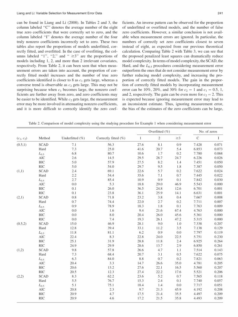
can be found in Liang and Li (2008). In Tables 2 and 3, thecolumn labeled ‘‘C’’ denotes the average number of the eighttrue zero coefficients that were correctly set to zero, and thecolumn labeled ‘‘I’’ denotes the average number of the fourtruly nonzero coefficients incorrectly set to zero. These twotables also report the proportions of models underfitted, cor-rectly fitted, and overfitted. In the case of overfitting, the col-umns labeled ‘‘1’’, ‘‘2,’’ and ‘‘ $3’’ are the proportions ofmodels including 1, 2, and more than 2 irrelevant covariates,respectively. From Table 2, it can been seen that when meas-urement errors are taken into account, the proportion of cor-rectly fitted model increases and the number of true zerocoefficients identified is closer to 8 as c1 gets large, whereas aconverse trend is observable as c2 gets large. This may not besurprising because when c1 becomes large, the nonzero coef-ficients are further away from zero, and zero coefficients maybe easier to be identified. While c2 gets large, the measurementerror may be more involved in attenuating nonzero coefficients,and it is more difficult to correctly identify the zero coef-

ficients. An inverse pattern can be observed for the proportionof underfitted or overfitted models, and the number of falsezero coefficients. However, a similar conclusion is not avail-able when measurement errors are ignored. In particular, thenumbers of correctly set zero coefficients closest to seveninstead of eight, as expected from our previous theoreticalcalculation. Comparing Table 2 with Table 3, we can see thatthe proposed penalized least squares can dramatically reducemodel complexity. In terms of model complexity, the SCAD, theHard, and the L0.5 procedures considering measurement erroroutperform the ones that do not consider measurement error byfurther reducing model complexity, and increasing the pro-portion of correctly fitted models. The gain in the propor-tion of correctly fitted models by incorporating measurementerror can be 10%, 20%, and 30% for c2 ¼ 1 and c1 ¼ 0.5, 1,and 2, respectively. The gain can be even more for c2 ¼ 2. Thisis expected because ignoring measurement error may lead toan inconsistent estimate. Thus, ignoring measurement error,the bias of the estimates of the zero coefficients can be large,

Table 2. Comparison of model complexity using the studying procedure for Example 1 when considering measurement error

(c1, c2) Method Underfitted (%) Correctly fitted (%)

Overfitted (%) No. of zeros

1 2 $3 C I

(0.5,1) SCAD 7.1 56.3 27.6 8.1 0.9 7.428 0.071Hard 7.3 25.0 41.6 20.7 5.4 6.853 0.073L0.5 6.8 80.7 10.6 1.7 0.2 7.780 0.068AIC 2.6 14.5 29.5 28.7 24.7 6.226 0.026BIC 5.0 57.9 27.5 8.2 1.4 7.451 0.050RIC 5.0 54.0 29.7 9.5 1.8 7.387 0.050

(1,1) SCAD 2.4 69.1 22.6 5.7 0.2 7.622 0.024Hard 2.2 54.4 35.6 7.1 0.7 7.445 0.022L0.5 2.7 85.4 10.9 0.9 0.1 7.842 0.030AIC 0.0 5.3 18.8 29.0 46.9 5.543 0.000BIC 0.1 26.0 36.5 24.8 12.6 6.701 0.001RIC 0.1 23.8 36.1 25.9 14.1 6.631 0.001






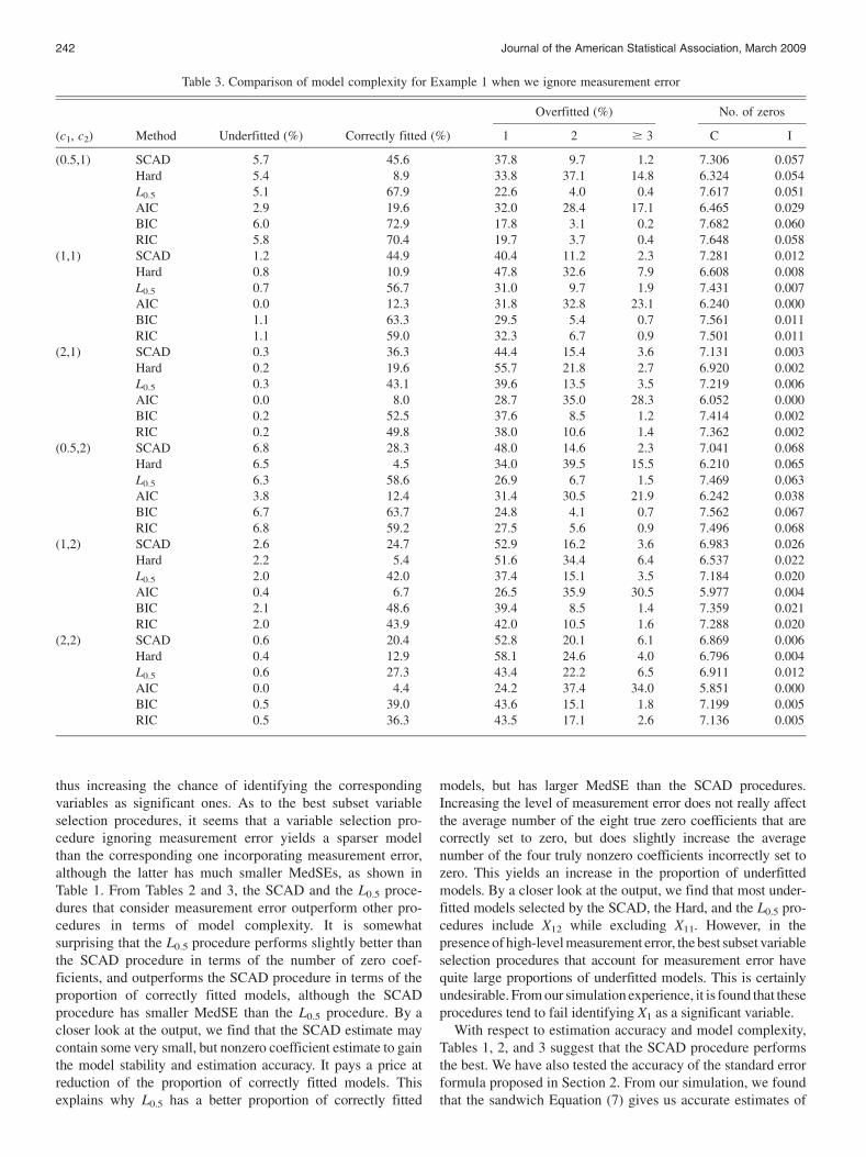
thus increasing the chance of identifying the correspondingvariables as significant ones. As to the best subset variableselection procedures, it seems that a variable selection pro-cedure ignoring measurement error yields a sparser modelthan the corresponding one incorporating measurement error,although the latter has much smaller MedSEs, as shown inTable 1. From Tables 2 and 3, the SCAD and the L0.5 proce-dures that consider measurement error outperform other pro-cedures in terms of model complexity. It is somewhatsurprising that the L0.5 procedure performs slightly better thanthe SCAD procedure in terms of the number of zero coef-ficients, and outperforms the SCAD procedure in terms of theproportion of correctly fitted models, although the SCADprocedure has smaller MedSE than the L0.5 procedure. By acloser look at the output, we find that the SCAD estimate maycontain some very small, but nonzero coefficient estimate to gainthe model stability and estimation accuracy. It pays a price atreduction of the proportion of correctly fitted models. Thisexplains why L0.5 has a better proportion of correctly fitted

models, but has larger MedSE than the SCAD procedures.Increasing the level of measurement error does not really affectthe average number of the eight true zero coefficients that arecorrectly set to zero, but does slightly increase the averagenumber of the four truly nonzero coefficients incorrectly set tozero. This yields an increase in the proportion of underfittedmodels. By a closer look at the output, we find that most under-fitted models selected by the SCAD, the Hard, and the L0.5 pro-cedures include X12 while excluding X11. However, in thepresence of high-level measurement error, the best subset variableselection procedures that account for measurement error havequite large proportions of underfitted models. This is certainlyundesirable. From our simulation experience, it is found that theseprocedures tend to fail identifying X1 as a significant variable.

With respect to estimation accuracy and model complexity,Tables 1, 2, and 3 suggest that the SCAD procedure performsthe best. We have also tested the accuracy of the standard errorformula proposed in Section 2. From our simulation, we foundthat the sandwich Equation (7) gives us accurate estimates of

Table 3. Comparison of model complexity for Example 1 when we ignore measurement error

(c1, c2) Method Underfitted (%) Correctly fitted (%)


1 2 $ 3 C I








standard errors, and the coverage probability of the confidenceinterval bj6zaSEðbjÞ is close to the nominal level, where za isthe 100 (1 � a/2)th percentile of the standard normal dis-tribution. To save space, we do not present the results here.

Example 2. We generate 1,000 datasets, each consisting ofn ¼ 200 random observations from model (1), in which the

covariates X, Z, and the baseline function n(Z) are exactly the

same as those in Example 1. The regression coefficient vector

b0 is taken to be the same as the one with c1 ¼ 1 in Example 1.

The first two components of X are measured with the error U,

while (e, UT) follows a contaminated normal distributions, (1�p)

N3 (0, s2I3) þ p N3(0, (10s)2I3) with p being the expected

proportion of contaminated data. Thus, (e, UT) follows an

elliptical distribution, which satisfies the assumptions of The-

orem 3. This contaminated model yields outlying data in a

more regular and predictable fashion than the one including

some outliers arbitrarily. To simultaneously examine the

impact of contamination proportion and the level of measure-

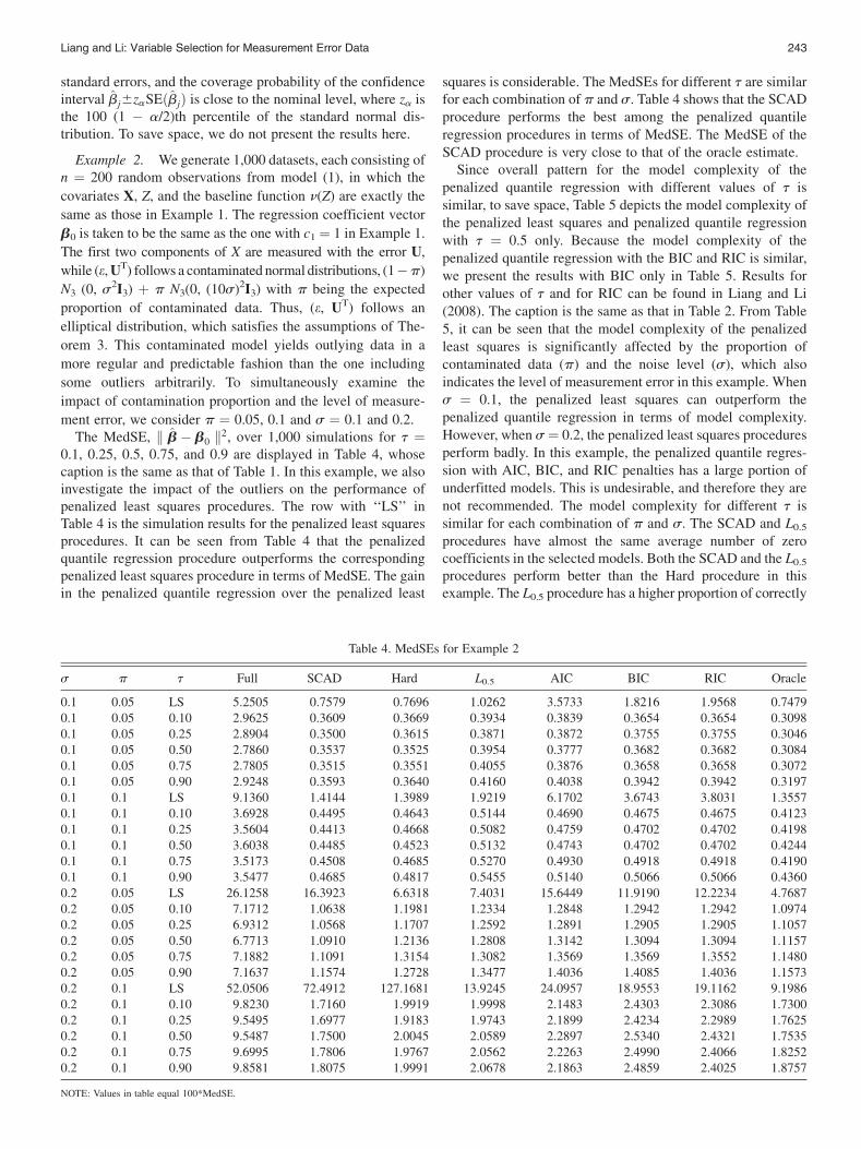
ment error, we consider p ¼ 0.05, 0.1 and s ¼ 0.1 and 0.2.The MedSE, k b� b0 k2, over 1,000 simulations for t ¼

0.1, 0.25, 0.5, 0.75, and 0.9 are displayed in Table 4, whosecaption is the same as that of Table 1. In this example, we alsoinvestigate the impact of the outliers on the performance ofpenalized least squares procedures. The row with ‘‘LS’’ inTable 4 is the simulation results for the penalized least squaresprocedures. It can be seen from Table 4 that the penalizedquantile regression procedure outperforms the correspondingpenalized least squares procedure in terms of MedSE. The gainin the penalized quantile regression over the penalized least

squares is considerable. The MedSEs for different t are similarfor each combination of p and s. Table 4 shows that the SCADprocedure performs the best among the penalized quantileregression procedures in terms of MedSE. The MedSE of theSCAD procedure is very close to that of the oracle estimate.

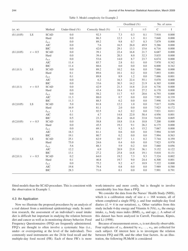
Since overall pattern for the model complexity of thepenalized quantile regression with different values of t issimilar, to save space, Table 5 depicts the model complexity ofthe penalized least squares and penalized quantile regressionwith t ¼ 0.5 only. Because the model complexity of thepenalized quantile regression with the BIC and RIC is similar,we present the results with BIC only in Table 5. Results forother values of t and for RIC can be found in Liang and Li(2008). The caption is the same as that in Table 2. From Table5, it can be seen that the model complexity of the penalizedleast squares is significantly affected by the proportion ofcontaminated data (p) and the noise level (s), which alsoindicates the level of measurement error in this example. Whens ¼ 0.1, the penalized least squares can outperform thepenalized quantile regression in terms of model complexity.However, when s ¼ 0.2, the penalized least squares proceduresperform badly. In this example, the penalized quantile regres-sion with AIC, BIC, and RIC penalties has a large portion ofunderfitted models. This is undesirable, and therefore they arenot recommended. The model complexity for different t issimilar for each combination of p and s. The SCAD and L0.5

procedures have almost the same average number of zerocoefficients in the selected models. Both the SCAD and the L0.5

procedures perform better than the Hard procedure in thisexample. The L0.5 procedure has a higher proportion of correctly

Table 4. MedSEs for Example 2

s p t Full SCAD Hard L0.5 AIC BIC RIC Oracle

0.1 0.05 LS 5.2505 0.7579 0.7696 1.0262 3.5733 1.8216 1.9568 0.74790.1 0.05 0.10 2.9625 0.3609 0.3669 0.3934 0.3839 0.3654 0.3654 0.30980.1 0.05 0.25 2.8904 0.3500 0.3615 0.3871 0.3872 0.3755 0.3755 0.30460.1 0.05 0.50 2.7860 0.3537 0.3525 0.3954 0.3777 0.3682 0.3682 0.30840.1 0.05 0.75 2.7805 0.3515 0.3551 0.4055 0.3876 0.3658 0.3658 0.30720.1 0.05 0.90 2.9248 0.3593 0.3640 0.4160 0.4038 0.3942 0.3942 0.31970.1 0.1 LS 9.1360 1.4144 1.3989 1.9219 6.1702 3.6743 3.8031 1.35570.1 0.1 0.10 3.6928 0.4495 0.4643 0.5144 0.4690 0.4675 0.4675 0.41230.1 0.1 0.25 3.5604 0.4413 0.4668 0.5082 0.4759 0.4702 0.4702 0.41980.1 0.1 0.50 3.6038 0.4485 0.4523 0.5132 0.4743 0.4702 0.4702 0.42440.1 0.1 0.75 3.5173 0.4508 0.4685 0.5270 0.4930 0.4918 0.4918 0.41900.1 0.1 0.90 3.5477 0.4685 0.4817 0.5455 0.5140 0.5066 0.5066 0.43600.2 0.05 LS 26.1258 16.3923 6.6318 7.4031 15.6449 11.9190 12.2234 4.76870.2 0.05 0.10 7.1712 1.0638 1.1981 1.2334 1.2848 1.2942 1.2942 1.09740.2 0.05 0.25 6.9312 1.0568 1.1707 1.2592 1.2891 1.2905 1.2905 1.10570.2 0.05 0.50 6.7713 1.0910 1.2136 1.2808 1.3142 1.3094 1.3094 1.11570.2 0.05 0.75 7.1882 1.1091 1.3154 1.3082 1.3569 1.3569 1.3552 1.14800.2 0.05 0.90 7.1637 1.1574 1.2728 1.3477 1.4036 1.4085 1.4036 1.15730.2 0.1 LS 52.0506 72.4912 127.1681 13.9245 24.0957 18.9553 19.1162 9.19860.2 0.1 0.10 9.8230 1.7160 1.9919 1.9998 2.1483 2.4303 2.3086 1.73000.2 0.1 0.25 9.5495 1.6977 1.9183 1.9743 2.1899 2.4234 2.2989 1.76250.2 0.1 0.50 9.5487 1.7500 2.0045 2.0589 2.2897 2.5340 2.4321 1.75350.2 0.1 0.75 9.6995 1.7806 1.9767 2.0562 2.2263 2.4990 2.4066 1.82520.2 0.1 0.90 9.8581 1.8075 1.9991 2.0678 2.1863 2.4859 2.4025 1.8757

NOTE: Values in table equal 100*MedSE.


fitted models than the SCAD procedure. This is consistent withthe observation in Example 1.

4.3 An Application

Now we illustrate the proposed procedures by an analysis ofa real dataset from a nutritional epidemiology study. In nutri-tion research, the assessment of an individual’s usual intakediet is difficult but important in studying the relation betweendiet and cancer as well as in monitoring dietary behavior. FoodFrequency Questionnaires (FFQ) are frequently administered.FFQ’s are thought to often involve a systematic bias (i.e.,under- or overreporting at the level of the individual). Twocommonly used instruments are the 24-hr food recall and themultiple-day food record (FR). Each of these FR’s is more

work-intensive and more costly, but is thought to involveconsiderably less bias than a FFQ.

We consider the data from the Nurses’ Health Study (NHS),which is a calibration study of size n ¼ 168 women, all ofwhom completed a single FFQ, y, and four multiple-day fooddiaries (Ji [ 4 in our notation), x1. Other variables from thisstudy include 4-day energy and Vitamin A (VA), x2, the energyintake, x3, body mass index (BMI), x4, and age, z. A subset ofthis dataset has been analyzed in Carroll, Freedman, Kipnis,and Li (1998).

Because of measurement errors, x1 is not directly observable.Four replicates of x1, denoted by w1, . . ., w4, are collected foreach subject. Of interest here is to investigate the relationbetween FFQ and FR, and the other four factors. As an illus-tration, the following PLMeM is considered

Table 5. Model complexity for Example 2

(s, p) Method Under-fitted (%) Correctly fitted (%)


1 2 $3 C I

(0.1,0.05) LS SCAD 0.0 92.3 7.3 0.3 0.1 7.918 0.000Hard 0.0 86.3 12.3 1.3 0.1 7.848 0.000L0.5 0.0 89.2 9.8 0.7 0.3 7.879 0.000AIC 0.0 7.6 16.5 26.0 49.9 5.286 0.000BIC 0.0 42.0 29.1 13.3 15.6 6.716 0.000

(0.1,0.05) t ¼ 0.5 SCAD 0.0 39.1 22.4 16.8 21.7 6.687 0.000Hard 0.0 39.4 20.3 8.0 32.3 5.835 0.000L0.5 0.0 53.6 14.0 8.7 23.7 6.674 0.000AIC 11.4 85.7 2.8 0.1 0.0 7.970 0.342BIC 11.4 88.6 0.0 0.0 0.0 8.000 0.342








y ¼ nðzÞ þX4

k¼1

bkxk þX4

u¼2

X4

y¼u

buyxuxy þ e; ð12Þ

and for each subject,

wj ¼ x1 þ uj; j ¼ 1; . . . ; 4;

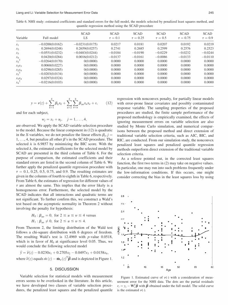
are observed. We apply the SCAD variable selection procedureto the model. Because the linear component in (12) is quadraticin the X-variables, we do not penalize the linear effects bj, j ¼1, . . ., 4, but penalize all other b’s in the SCAD procedure. Theselected l is 6.9857 by minimizing the BIC score. With theselected l, the estimated coefficients for the selected model bySCAD are presented in the third column of Table 6. For thepurpose of comparison, the estimated coefficients and theirstandard errors are listed in the second column of Table 6. Wefurther apply the penalized quantile regression procedure witht ¼ 0.1, 0.25, 0.5, 0.75, and 0.9. The resulting estimates aregiven in the columns of fourth to eighth in Table 6, respectively.From Table 6, the estimates of regression for different values oft are almost the same. This implies that the error likely is ahomogeneous error. Furthermore, the selected model by theSCAD indicates that all interactions and quadratic terms arenot significant. To further confirm this, we construct a Wald’stest based on the asymptotic normality in Theorem 2 withoutinvolving the penalty for hypothesis:

H0 : buy ¼ 0; for 2 # u # y # 4 versus

H1 : buy 6¼ 0; for 2 # u # y # 4:

From Theorem 2, the limiting distribution of the Wald testfollows a chi-square distribution with 6 degrees of freedom.The resulting Wald’s test is 12.4969 with p-value 0.0518,which is in favor of H0 at significance level 0.05. Thus, wewould conclude the following selected modelby ¼ bnðzÞ � 0:0230x1 þ 0:2705x2 � 0:0497x3 þ 0:0158x4;

where bnðzÞ equals m ðzÞ � mwðzÞTbb and is depicted in Figure 1.

5. DISCUSSION

Variable selection for statistical models with measurementerrors seems to be overlooked in the literature. In this article,we have developed two classes of variable selection proce-dures, the penalized least squares and the penalized quantile

regression with nonconvex penalty, for partially linear modelswith error-prone linear covariates and possibly contaminatedresponse variable. The sampling properties of the proposedprocedures are studied, the finite sample performance of theproposed methodology is empirically examined, the effects ofignoring measurement errors on variable selection are alsostudied by Monte Carlo simulation, and numerical compar-isons between the proposed method and direct extension oftraditional variable selection criteria, such as AIC, BIC, andRIC, are conducted. From our simulation study, the nonconvexpenalized least squares and penalized quantile regressionmethods outperform direct extension of the traditional variableselection criteria.

As a referee pointed out, in the corrected least squaresfunction, the first two terms in (2) may take on negative values.In particular, one may run into such problems frequently underthe low-information conditions. If this occurs, one mightconsider correcting the bias in the least squares loss by using

Table 6. NHS study: estimated coefficients and standard errors for the full model, the models selected by penalized least squares method, andquantile regression method using the SCAD procedure

Variable Full modelSCAD SCAD SCAD SCAD SCAD SCAD

LS t ¼ 0.1 t ¼ 0.25 t ¼ 0.5 t ¼ 0.75 t ¼ 0.9

x1 �0.0200(0.0162) �0.0231(0.0175) 0.0217 0.0181 0.0207 0.0192 0.0219x2 0.2694(0.0248) 0.2659(0.0257) 0.2741 0.2685 0.2599 0.2576 0.2523x3 �0.0551(0.0232) �0.0483(0.0244) �0.0184 �0.0190 �0.0229 �0.0232 �0.0244x4 0.0420(0.0284) 0.0016(0.0212) �0.0137 �0.0161 �0.0086 �0.0133 �0.0110x2

2 �0.0264(0.0170) 0(0.0000) 0.0000 0.0000 0.0000 0.0000 0.0000x2x3 0.0060(0.0227) 0(0.0000) 0.0000 0.0000 0.0000 0.0000 0.0000x2x4 0.0298(0.0285) 0(0.0000) 0.0000 0.0000 0.0000 0.0000 0.0000x3

2 �0.0203(0.0134) 0(0.0000) 0.0000 0.0000 0.0000 0.0000 0.0000x3x4 0.0297(0.0324) 0(0.0000) 0.0000 0.0000 0.0000 0.0000 0.0000x4

2 �0.0216(0.0103) 0(0.0000) 0.0000 0.0000 0.0000 0.0000 0.0000

Figure 1. Estimated curve of n(�) with a consideration of meas-urement error for the NHS data. The dots are the partial residualsri ¼ yi �WT

i b with b obtained under the full model. The solid curveis the estimated n(�).


the orthogonal regression method, as in (10). Further study isneeded in this area.

As demonstrated in our simulation, the proposed proceduresperform reasonably well with moderate sample sizes. As a ref-eree noted, it is of interest to study variable selection for largedimension, small sample size measurement error data. We haveconducted some empirical study via Monte Carlo simulation.From our limited experience, one should be cautious in applyingour methods when the number of predictors is close to thesample size. In such situations, the proposed procedures likelyresult in an underfitted model excluding some significant pre-dictors. There are some recent developments on variableselection for linear regression models with large dimension andsmall sample size data (Candes and Tao 2007; Fan and Lv 2008).Further research is needed for measurement error data.

APPENDIX: ASSUMPTIONS ANDTECHNICAL DETAILS

The following regularity conditions are needed for Theo-rems 1–3. They may not be the weakest ones.

Regularity Conditions:

(a) SX|Z is a positive-definite matrix, E(e |X, Z) ¼ 0, andE(|e|3|X, Z) < ‘;(b) The bandwidths in estimating mw(z) and my(z) are oforder n�1/5;(c) K (�) is a bounded symmetric density function withcompact support and satisfiesð

KðuÞ du ¼ 1;

ðKðuÞu du ¼ 0; and

ðu2KðuÞ du ¼ 1;

(d) The density function of Z, fZ(z), and the density functionof (Y, Z) are bounded away from 0 and have bounded con-tinuous second derivative;(e) my(z) and mw(z) have bounded and continuous secondderivatives.

We first point out a fact, which is assured by Conditions (b)–(e), that the local polynomial estimates of my (�) and mw (�)satisfy

supzjbmyðzÞ � myðzÞj ¼ opðn�1=4Þ; and sup

zjbmw; jðzÞ � mw; jðzÞj

¼ opðn�1=4ÞðA:1Þ

for j ¼ 1, . . ., d, where mw, j(�) and bmw; jð�Þ are the jth compo-nents of mw(�) and bmwð�Þ, respectively. See Mack and Silver-man (1982) for a detailed discussion of the proof of (A.1),which will repeatedly be used in our proof. Let |ji| ¼ maxi|ji|for any sequence {ji}.

Lemma A.1

Assume that random variables ai(Wi, Zi, Yi) and ci (Wi, Zi,Yi), denoted by ai and ci, satisfy ai(Wi, Zi, Yi) [ 1 or Eai¼ 0 and|ci| ¼ op(n–1/4). ThenXn

i¼1

aici-i ¼ opðffiffiffinpÞ;

where -i are independent variables with mean zero and finitevariance.

The lemma can be shown along the same lines as those ofLemma A.5 of Liang, et al. (1999). We omit the details.

A.1 Proof of Theorem 1

The strategy to prove Theorem 1 is similar to those ofTheorems 1 and 2 of Fan and Li (2001). Only the key ideas areoutlined below.

Let an ¼ n�1/2. We show that, for any given z > 0, thereexists a large constant C such that

P infkvk¼C

LPðSuu;b0 þ anvÞ>LPðSuu;b0Þ�

$ 1� z: ðA:2Þ

Denote

JnðvÞ ¼Xn

i¼1

bYi �cW Ti ðb0 þ anvÞ

n o2

� bYi �cW Ti b0

�2� �

� nfðb0 þ anvÞTSuðb0 þ anvÞ � bT0 Sub0g:

Then, Jn(v) can be represented as

JnðvÞ ¼ �2an

Xn

i¼1

bYicW T

i �cW Ti b0

cW Ti þ b T

0 Su

�v

þ na2nvTðn�1cWi

cW Ti � SuÞv:

ðA:3Þ

We next calculate the order of the first term. Note thatXn

i¼1

ðbYicW T

i �cW Ti b0

cW Ti þ b T

0 SuÞ

¼Xn

i¼1

ðbYi � eYiÞ ðcWi �fWiÞT þXn

i¼1

ðbYi � eYiÞfWTi

þXn

i¼1

eYiðcWi �fWiÞT þXn

i¼1

ðeYi �fWTi b0fWT

i þ bT0 SuÞ

�Xn

i¼1

ðcWi �fWiÞTb0ðcWi �fWiÞT �Xn

i¼1

fWTi b0ðcWi �fWiÞT

�Xn

i¼1

ðcWi �fWiÞTb0fWT

i :

It is seen that the first and fifth terms are op(n1/2) by (A.1).Using Lemma A.1 yields that the second, third, sixth, andseventh terms are Op(n1/2). Furthermore, E eYi ¼ 0, EfWi ¼ 0. Itfollows from the central limit theorem that the fourth term isOp(n1/2). Therefore, the first term in (A.3) is of the orderOpð

ffiffiffinp

anÞ ¼ Opð1Þ as an ¼ O(n�1/2). Taking C large enough,the first term in (A.3) is dominated by the second term in (A.3)as n�1cWi

cW Ti � Su ! EeXTeX in probability.

Note that

DnðvÞ[LPðSuu;b0 þ anvÞ � LPðSuu;b0Þ

$ JnðvÞ þ nXs

j¼1

fplnðjbj0 þ anyjjÞ � pln

ðjbj0jÞg;

ðA:4Þwhere s is the dimension of b10.

As shown in Fan and Li (2001), the second term of (A.4) isbounded by the second term in (A.3) under the assumption of


an¼Op(n�1/2) and bn! 0. Thus, by taking C large enough, thesecond term in (A.3) dominates both the first term in (A.3) andthe second term in (A.4). This proves Part 1.

We now prove the sparsity. It suffices to show that for anygiven b1 satisfying jj k b1 � b10 k¼ Opðn�1=2Þ and j ¼ s þ 1,. . ., d, such that @LPðSuu;bÞ=@bj > 0 for 0 < bj < en ¼ Cn�1/2,and @LPðSuu;bÞ=@bj < 0 for � en < bj < 0.By the Taylor expansion, we have

@LPðSuu;bÞ@bj

¼ � 2½Yi � bmyðZiÞ � fWi � bmwðZiÞgTb�

fWi � bmwðZiÞgj þ np0ljðjbjjÞsgnðbjÞ:

The first term can be shown to be Op(n�1/2) by (A.1) and that b1�b10 ¼ Op(n�1/2). Recall that n1/2l ! ‘, and lim infn!‘

lim infu!0 þ p0lðuÞ=l > 0: We know that the sign of @LP

ðSuu;bÞ=@bj is determined by that of bj, and is negative for 0 < bj

< en and positive for � en > bj > 0. It follows that b2 ¼ 0.We now prove 2(b) by using the results of Newey (1994) to

show the asymptotic normality of b1. Note that the estimatorsbb1 based on the penalized likelihood function given in (2) areequivalent to the solution of the estimating equation:

Xn

i¼1

Fðbmw1; bmy;b1; Yi;Wi1; ZiÞ � nz1 ¼ 0; ðA:5Þ

where Fðmw1;my;b1; Y ;W1; ZÞ ¼ W1 �mw1ðZÞf g Y � my

�ðZÞ � W1 �mw1ðZÞf gTb1� � Suu1b1 and z1 ¼ fp0lðjb1jÞsgnðb1Þ; . . . ; p0lðjbsjÞsgnðbsÞg

T.

It follows from (A.1) that jbmw1ðZÞ �mw1ðZÞj ¼ opðn�1=4Þand bmyðZÞ � myðZÞ ¼ opðn�1=4Þ.Thus, Assumption 5.1(ii) in Newey (1994) holds. Let

D ðm�w1 �mw1;m�y � myÞ ¼

@F

@mw1ðm�w1 �mw1Þ þ

@F

@myðm�y

� myÞ;where @F / @mw1 and @F / @my are the Frechet derivatives.A direct but cumbersome calculation derives that Eð@F=@mw1Þ ¼ 0 and Eð@F=@myÞ ¼ 0. Furthermore,

jFðm�w1;m�y ;b1; Y ;W1; ZÞ �Fðmw1;my;b1; Y ;W1; ZÞ�

Dðm�w1 �mw1;m�y � myÞj ¼ Op jm�w1 �mw1j2 þ jm�y � myj2

�:

ðA:6Þ

This indicates that Assumption 5.1(i) in Newey (1994) isvalid. Furthermore, it can be seen by noting the expression ofD(�, �) that Assumption 5.2 of Newey (1994) is also valid. Inaddition, it follows from the previous statements that for any

m�w1;m�y

�;

E Dðm�w1 �mw1;m�y � myÞ

n o¼ 0;

and Newey’s Assumption 5.3, a(T) ¼ 0, holds. By Lemma 5.1in Newey (1994), it follows that bb1 has the same distribution asthe solution to the equation:

0 ¼Xn

i¼1

Fðmw1;my;b1; Yi;Wi1; ZiÞ � nz1: ðA:7Þ

A direct simplification yields that

eX11eXT

11

ffiffiffinpðbb1 � b01Þ þ n1=2b ¼ n�1=2

Xn

i¼1

feXi1ðei � UTi b10Þ

þ Uiei þðUiUTi � Suu1Þb10g:

This completes the proof.

A.2 Proof of Theorem 3

To prove Theorem 3, we need a fact regarding ellipticaldistributions. Let q be a random vector. It is said that q followsan elliptical distribution if its characteristic function is of theform

EfexpðitTqÞg ¼ exp ðimTtÞf ðtTLtÞ:

It is known that E(q) ¼ m and cov(q ¼ {�2f9(0)}L (Fang,et al. 1990). Furthermore, we have that if m ¼ 0, then for anyconstant vector b 6¼ 0,

q1¼dbTqffiffiffiffiffiffiffiffiffiffiffiffiffiffiffiffiffiffiffiffiffi

bTLb=L11

p ; ðA:8Þ

where q1 is the first element of q, and L11 is the (1,1)-elementof L, and R1¼

dR2 means R1 and R2 have the same distribution.

(A.8) can be easily shown by calculating the characteristicfunctions of the random variables on each side of (A.8).

Now we prove Theorem 3. We can use the arguments similar tothose for Theorem 1 to prove Part 1 and 2(a), and omit the details.We now finish the proof of Part 2(b) in three steps. For notational

simplicity, write bai ¼cWi þ bYi �cW Ti b=1þ bTCuub � b, bci ¼

ctðbYi �cWTi b=


pÞ, ai ¼fWi þ ei � UT

i b=1þ bT

Cuub � b, and ci ¼ ct ei � UTi b=


p �, where ct is

the derivative of rt.Step 1. It is straightforward to verify that

max1 # i # n

jbai � aij ¼ opðn�1=4Þ; max1 # i # n

jbci � cij¼ opðn�1=4Þ: ðA:9Þ

Note that both ai and ci are sequences of iid variables withmean zero and finite variances. It follows from (A.9) andLemma A.1 thatX

i

baibci �X

i

aici ¼X

i

ðbci � ciÞðbai � aiÞ þX

i

ðbci � ciÞai

�Xðbai � aiÞci ¼ opðn1=2Þ:

This argument indicates that the estimator bt has the sameasymptotic distribution as that of the estimators constructed byminimizing the objective function:

Xn

i¼1

rt

eYi �fWTi bffiffiffiffiffiffiffiffiffiffiffiffiffiffiffiffiffiffiffiffiffiffiffiffi

1þ bTCuubp !

þ nXd

j¼1

pljðjbjjÞ ¼

defQðbÞ

þ nXd

j¼1

pljðjbjjÞ

with respect to b.Step 2. Note that the loss function rt is differentiable

everywhere except at the point of zero. The directional deriv-atives of Q(b) at the solution bt are all nonnegative, whichimplies that


Xi

eWi1 þeYi �fWT

i1b1

1þ bT1 C11b1

b1

!ct

eYi �fWTi1b1ffiffiffiffiffiffiffiffiffiffiffiffiffiffiffiffiffiffiffiffiffiffiffiffiffiffi

1þ bT1 C11b1

q0B@

1CA� nz1

ffiffiffiffiffiffiffiffiffiffiffiffiffiffiffiffiffiffiffiffiffiffiffiffiffiffi1þ bT

1 C11b1

q¼ Opð

XfWi1ÞðA:10Þ

at b1 ¼ bt1.Step 3. We apply a similar idea to Corollary 2.2 of He and

Shao (1996) for M-estimators to complete the proof by ver-ifying the assumptions needed for the Corollary and setting r ¼ 1,An ¼ lmax (Jq)n, and Dn ¼ nf ðqtÞð1þ bT

10C11b10Þ�1=2SXjZ.

Here lmax (Jq) denotes the maximum eigenvalue of Jq, whichis equal to

Efc2tðjÞeX�2

1 g þ cov U11 þjb10ffiffiffiffiffiffiffiffiffiffiffiffiffiffiffiffiffiffiffiffiffiffiffiffiffiffiffiffiffi

1þ bT10C11b10

q0B@

1CActðjÞ

8><>:9>=>;:

Furthermore, let ji ¼ ðei � UTi1b10Þ=


10C11b10

q� qt.

With the assumption of elliptical symmetry on (e, UT) and by(A8), ji and ei � qt have the same distribution. It then followsfrom an argument similar to that for Corollary 2.2 of He andShao (1996) thatffiffiffi

np

f ðqtÞð1þ bT10C11b10Þ1=2

SXjZðbt1 � b10Þ

þ nb


10C11b10

q¼ 1ffiffiffi

np

Xn

i¼1

eXi1 þ Ui1 þjib10ffiffiffiffiffiffiffiffiffiffiffiffiffiffiffiffiffiffiffiffiffiffiffiffiffiffiffiffiffi

1þ bT10C11b10

q0B@

1CActðjiÞ þ opð1Þ:

The proof of Theorem 3 is completed by using the central limittheorem with a direct calculation.

[Received September 2006. Revised November 2008.]

REFERENCES

Akaike, H. (1973), ‘‘Maximum Likelihood Identification of Gaussian Autor-egressive Moving Average Models,’’ Biometrika, 60, 255–265.

Bellman, R. (1961), Adaptive Control Processes: A Guided Tour, Princeton, NJ:Princeton University Press.

Berger, J., and Percchi, L. (1996), ‘‘The Intrinsic Bayes Factor for ModelSelection and Prediction,’’ Journal of the American Statistical Association,91, 109–122.

Breiman, L. (1996), ‘‘Heuristics of Instability and Stabilization in ModelSelection,’’ The Annals of Statistics, 24, 2350–2383.

Bunea, F. (2004), ‘‘Consistent Covariate Selection and Post Model SelectionInference in Semiparametric Regression,’’ The Annals of Statistics, 32, 898–927.

Bunea, F., and Wegkamp, M. (2004), ‘‘Two-stage Model Selection Procedures inPartially Linear Regression,’’ The Canadian Journal of Statistics, 32, 105–118.

Candes, E., and Tao, T. (2007), ‘‘The Dantzig Selector: Statistical EstimationWhen p is Much Larger Than n’’ (with discussion),’’ The Annals of Statistics,35, 2313–2404.

Carroll, R. J., Freedman, L. S., Kipnis, V., and Li, L. (1998), ‘‘A New Class ofMeasurement Error Models, With Applications to Estimating the Dis-tribution of Usual Intake,’’ The Canadian Journal of Statistics, 26, 467–477.

Carroll, R. J., Ruppert, D., Stefanski, L. A., and Crainiceanu, C. M. (2006),Measurement Error in Nonlinear Models (2nd ed), New York: Chapman and Hall.

Cheng, C. L., and Van Ness, J. W. (1999), Statistical Regression With Meas-urement Error, New York: Oxford University Press Inc.

Fan, J., and Gijbels, I. (1996), Local Polynomial Modelling and Its Applica-tions, New York: Chapman and Hall.

Fan, J., and Li, R. (2001), ‘‘Variable Selection via Nonconcave PenalizedLikelihood and Its Oracle Properties,’’ Journal of the American StatisticalAssociation, 96, 1348–1360.

——— (2004), ‘‘New Estimation and Model Selection Procedures for Semi-parametric Modeling in Longitudinal Data Analysis,’’ Journal of theAmerican Statistical Association, 99, 710–723.

Fan, J., and Lv, J. (2008), ‘‘Sure Independence Screening for Ultra-HighDimensional Feature Space’’ (with discussions),’’ Journal of the RoyalStatistical Society, Ser. B., 70, 849–911.

Fang, K. T., Kotz, S., and Ng, K. W. (1990), Symmetric Multivariate andRelated Distributions, London: Chapman and Hall.

Foster, D. P., and George, E. I. (1994), ‘‘The Risk Inflation Criterion forMultiple Regression,’’ The Annals of Statistics, 22, 1947–1975.

Frank, I. E., and Friedman, J. H. (1993), ‘‘A Statistical View of Some Che-mometrics Regression Tools,’’ Technometrics, 35, 109–148.

Fuller, W. A. (1987), Measurement Error Models, New York: John Wiley.George, E. I., and McCulloch, R. E. (1993), ‘‘Variable Selection via Gibbs

Sampling,’’ Journal of the American Statistical Association, 88, 881–889.Gleser, L. J. (1992), ‘‘The Importance of Assessing Measurement Reliability in

Multivariate Regression,’’ Journal of the American Statistical Association,419, 696–707.

He, X., and Liang, H. (2000), ‘‘Quantile Regression Estimates for a Class ofLinear and Partially Linear Errors-in-Variables Models,’’ Statistica Sinica,10, 129–140.

He, X., and Shao, Q. (1996), ‘‘A General Bahadur Representation of M-estimators and Its Application to Linear Regression With NonstochasticDesigns,’’ The Annals of Statistics, 24, 2608–2630.

Hocking, R. R. (1976), ‘‘The Analysis and Selection of Variables in LinearRegression,’’ Biometrics, 32, 1–49.

Hoeting, J. A., Madigan, D., Raftery, A. E., and Volinsky, C. T. (1999),‘‘Bayesian Model Averaging: A Tutorial,’’ Statistical Science, 14, 382–417.

Hunter, D. R., and Lange, K. (2000), ‘‘Quantile Regression via an MM Algo-rithm,’’ Journal of Computational and Graphical Statistics, 9, 60–77.

Hunter, D., and Li, R. (2005), ‘‘Variable Selection Using MM Algorithms,’’ TheAnnals of Statistics, 33, 1617–1642.

Jiang, W. X. (2007), ‘‘Bayesian Variable Selection for High DimensionalGeneralized Linear Models: Convergence Rates for the Fitted Densities,’’The Annals of Statistics, 35, 1487–1511.

Koenker, R. (2005), Quantile Regression, New York: Cambridge University Press.Li, R., Fang, K. T., and Zhu, L. X. (1997), ‘‘Some Probability Plots to Test

Spherical and Elliptical Symmetry,’’ Journal of Computational and Graph-ical Statistics, 6, 435–450.

Liang, H., Hardle, W., and Carroll, R. J. (1999), ‘‘Estimation in a Semi-parametric Partially Linear Errors-in-Variables Model,’’ The Annals of Sta-tistics, 27, 1519–1935.

Liang, H., and Li, R. (2008): ‘‘Variable Selection for Partially Linear ModelsWith Measurement Errors.’’ Technical Report. Department of Biostatistics,University of Rochester Medical Center, Rochester, NY .

Liang, H., Wang, S. J., and Carroll, R. J. (2007), ‘‘Partially Linear Models WithMissing Response Variables and Error-prone Covariates,’’ Biometrika, 94,185–198.

Lindley, D. B. (1947), ‘‘Regression Lines and the Functional Relationship,’’Journal of the Royal Statistical Society, Ser. B, 9, 219–244.

Ma, Y. Y., and Carroll, R. J. (2006), ‘‘Locally Efficient Estimators for Semi-parametric Models With Measurement Error,’’ Journal of the AmericanStatistical Association, 101, 1465–1474.

Mack, Y., and Silverman, B. (1982), ‘‘Weak and Strong Uniform Consistencyof Kernel Regression Estimates,’’ Zeitschrift fur Wahrscheinlichkeitstheorieund Verwandte Gebiete, 60, 405–415.

Madansky, A. (1959), ‘‘The Fitting of Straight Lines When Both Variables AreSubject to Error,’’ Journal of the American Statistical Association, 54, 173–205.

Mitchell, T. J., and Beauchamp, J. J. (1988), ‘‘Bayesian Variable Selection inLinear Regression,’’ Journal of the American Statistical Association, 83,1023–1032.

Newey, W. K. (1994), ‘‘The Asymptotic Variance of Semiparametric Estima-tors,’’ Econometrica, 62, 1349–1382.

Pan, W. Q., Zeng, D. L., and Lin, X. H. (2008), ‘‘Estimation in SemiparametricTransition Measurement Error Models for Longitudinal Data,’’ Biometrics.,forthcoming in.

Raftery, A. E., Madigan, D., and Hoeting, J. A. (1997), ‘‘Bayesian ModelAveraging for Linear Regression Models,’’ Journal of the American Stat-istical Association, 92, 179–191.

Ruppert, D., Sheather, S. J., and Wand, M. P. (1995), ‘‘An Effective BandwidthSelector for Local Least Squares Regression,’’ Journal of the AmericanStatistical Association, 90, 1257–1270.

Schwarz, G. (1978), ‘‘Estimating the Dimension of a Model,’’ The Annals ofStatistics, 6, 461–464.

Tibshirani, R. (1996), ‘‘Regression Shrinkage and Selection via the LASSO,’’Journal of the Royal Statistical Society, Ser. B, 58, 267–288.

Wang, H., Li, R., and Tsai, C. L. (2007), ‘‘Tuning Parameter Selectors for theSmoothly Clipped Absolute Deviation Method,’’ Biometrika, 94, 553–568.

Wang, N. S., Lin, X. H., Gutierrez, R. G., and Carroll, R. J. (1998), ‘‘Bias Analysisand SIMEX Approach in Generalized Linear Mixed Measurement ErrorModels,’’ Journal of the American Statistical Association, 93, 249–261.


Documents

Variable Selection for Partially Linear Models With ...stefanski/mem_reports_2011/variable selection...Variable Selection for Partially Linear Models ... X, Z) ¼ 0, U is the measure-