Embed Size (px)
Citation preview

Full Terms & Conditions of access and use can be found athttp://www.tandfonline.com/action/journalInformation?journalCode=ilab20
Download by: [Politecnico di Milano Bibl] Date: 24 May 2016, At: 03:46
Critical Reviews in Clinical Laboratory Sciences
ISSN: 1040-8363 (Print) 1549-781X (Online) Journal homepage: http://www.tandfonline.com/loi/ilab20
Generation of data on within-subject biologicalvariation in laboratory medicine: An update
Federica Braga & Mauro Panteghini
To cite this article: Federica Braga & Mauro Panteghini (2016) Generation of data on within-subject biological variation in laboratory medicine: An update, Critical Reviews in ClinicalLaboratory Sciences, 53:5, 313-325, DOI: 10.3109/10408363.2016.1150252
To link to this article: http://dx.doi.org/10.3109/10408363.2016.1150252
Accepted author version posted online: 08Feb 2016.Published online: 14 Mar 2016.
Submit your article to this journal
Article views: 47
View related articles
View Crossmark data

http://informahealthcare.com/labISSN: 1040-8363 (print), 1549-781X (electronic)
Crit Rev Clin Lab Sci, 2016; 53(5): 313–325! 2016 Informa UK Limited, trading as Taylor & Francis Group. DOI: 10.3109/10408363.2016.1150252
REVIEW ARTICLE
Generation of data on within-subject biological variation in laboratorymedicine: An update
Federica Braga and Mauro Panteghini
Centre for Metrological Traceability in Laboratory Medicine (CIRME), University of Milan, Milano, Italy
Abstract
In recent decades, the study of biological variation of laboratory analytes has receivedincreased attention. The reasons for this interest are related to the potential practicalapplications of such knowledge. Biological variation data allow the derivation of importantparameters for the interpretation and use of laboratory tests, such as the index of individualityfor the evaluation of the utility of population reference intervals for the test interpretation, theestimate of significant change in a timed series of results of an individual, the number ofspecimens required to obtain an accurate estimate of the homeostatic set point of the analyteand analytical performance specifications that assays should fulfill for their application in theclinical setting. It is, therefore, essential to experimentally derive biological variationinformation in an accurate and reliable way. Currently, a dated guideline for the biologicalvariation data production and a more recent checklist to assist in the correct preparation ofpublications related to biological variation studies are available. Here, we update and integrate,with examples, the available guideline for biological variation data production to helpresearchers to comply with the recommendations of the checklist for drafting manuscripts onbiological variation. Particularly, we focus on the distribution of the data, an essential aspect tobe considered for the derivation of biological variation data. Indeed, the difficulty in derivingreliable estimates of biological variation for those analytes, the measured concentrations ofwhich are not normally distributed, is more and more evident.
Abbreviations: ANOVA: analysis of variance; CA-125: carbohydrate antigen 125; CgA:chromogranin A; CI95%: confidence intervals at 95%; CRP: C-reactive protein; cTnT: cardiactroponin T; CVA: analytical coefficient of variation; CVG: between-subject biological coefficientvariation; CVI: within-subject biological coefficient of variation; CVT: within-subject totalcoefficient of variation; DCCT: Diabetes Control and Complications Trial; EFLM: EuropeanFederation of Clinical Chemistry and Laboratory Medicine; FLC: immunoglobulin-free k and �light chains; HbA1c: glycated hemoglobin; HE4: human epididymis protein 4; ICC: intraclasscorrelation coefficient; IFCC: International Federation of Clinical Chemistry and LaboratoryMedicine; IH: index of heterogeneity; II: index of individuality; IQC: internal quality controlprogram; IUPAC: International Union of Pure and Applied Chemistry; LoD: limit of detection;ME: IFCC-NGSP master equation; n: number of specimens required for an analyte to ensure thatthe mean result be within desired percentage closeness to the individual’s homeostatic setpoint; NGSP: National Glycohemoglobin Standardization Program; NSE: neuron-specificenolase; P1: baseline result; P2: the following value that was significantly lower or higherthan P1; RCV: reference change value; RI: reference interval; S2
A: average within-run analyticalvariance; S2
G: between-subject biological variance; S2I: average within-subject biological
variance; S2I+A: average within-subject total variance; S2
T: total variance of all measurements;SEQC: Spanish Society of Clinical Chemistry and Molecular Pathology; STARD: Standards forReporting of Diagnostic Accuracy; TE: total error
Keywords
Intra-individual biological variation,inter-individual biological variation,within-subject biological variation,between-subject biological variation,normality test, analytical goals, index ofindividuality, reference change value
History
Received 9 October 2015Revised 10 December 2015Accepted 1 February 2016Published online 10 March 2016
Referees: Dr. Alan Wu, Professor of Laboratory Medicine, Chief of Clinical Chemistry Laboratory, San Francisco General Hospital & Trauma Center,San Francisco, CA, USA; Dr. Per Hyltoft Petersen, NOKLUS, Section for General Practice, University of Bergen, Bergen, Norway; Dr. Niels Jonker,BioMolecular Analysis, Department of Chemistry and Pharmaceutical Sciences, Faculty of Sciences, VU University Amsterdam, The Netherlands.
Address for correspondence: Federica Braga, Centre for Metrological Traceability in Laboratory Medicine, UOC Patologia Clinica, Ospedale ‘LuigiSacco’, University of Milan, Via G.B. Grassi 74, Milano, Italy. E-mail: [email protected]
Dow
nloa
ded
by [
Polit
ecni
co d
i Mila
no B
ibl]
at 0
3:46
24
May
201
6

Biological variation and derived indices
Introduction to biological variation
The total variation (CVT) of a laboratory result is made up
of three components, namely, preanalytical variation, ana-
lytical variation (CVA) and within-subject biological vari-
ation (CVI)1. The preanalytical variation concerns all phases
covering the preparation of the subject for sampling, and the
collection, transport, storage and handling of biological
samples. It can be assumed that, once all potential
preanalytical factors have been identified, they can be
minimized and the contribution of the preanalytical variation
component to CVT can be considered negligible. CVA is
associated with the analytical performance in terms of
measurement errors. This variability should be strictly
controlled, but, unlike the preanalytical variation, it cannot
be completely removed. Finally, CVI represents the physio-
logical changes of analyte concentration that occurs in a
specified biological fluid in each individual due to bio-
logical factors1. At each moment, the concentration of a
constituent in a biological fluid, e.g. blood or urine, in a
single individual is the result of dynamic control. This
control is due to mechanisms that tend to maintain the
analyte concentration around an average value that is
optimal for the organism, namely the ‘‘homeostatic set
point.’’ CVI reflects this random fluctuation of the analyte
concentration around the homeostatic set point. In contrast,
the between-subject biological variation (CVG) expresses the
difference among homeostatic set points for the same
analyte in different individuals under the same physiological
conditions1. By definition, the biological variation compo-
nents are not reducible and are typically associated with a
given analyte. As CVI tends to vary from individual to
individual, in general, the average of CVI values derived in a
group of individuals is considered. This should be obtained
experimentally through a rigorous experimental protocol that
includes the elimination of preanalytical variation, the
careful estimate of CVA, and the robust statistical derivation
of CVI and CVG, expressed as coefficient of variation.
Biological variation studies of different body constituents
have received increasing attention in recent decades because
of the potential practical application of such knowledge.
Biological variation data are now considered a required
element to judge the potential clinical significance of a
biomarker.
Applications of data on biological variation
Biological variation data for an analyte permits the derivation
of important information for the correct application and
clinical interpretation of its measurement2. In particular, the
evaluation of utility of population reference intervals (RIs) for
the interpretation of test results, the estimate of the signifi-
cance of changes of results in an individual and the
calculation of the number of specimens required for an
analyte to ensure that the mean result is within the desired
closeness to the individual’s homeostatic set point (n) can be
derived. Finally, it is possible to derive analytical performance
specifications for a given measurement to assess its suitability
for clinical use.
Analytical performance specifications
Defining analytical performance specifications for each
analyte measurement is essential to make its determination
clinically usable and to ensure that the measurement error
does not have an impact on the result3. In a conference held in
1999 in Stockholm under the auspices of the International
Federation of Clinical Chemistry and Laboratory Medicine
(IFCC) and International Union of Pure and Applied
Chemistry (IUPAC), a hierarchy of sources for deriving the
analytical goals of a laboratory measurement and defining
quality specifications in laboratory medicine was defined4. In
2014, a follow-up conference held in Milan revisited the
Stockholm consensus and investigated the extent to which the
originally advocated hierarchy was still valid or the need to
change or expand it5. Although the essence of the hierarchy
established in Stockholm was still supported, new perspec-
tives prompted its simplification and explanatory additions.
The recommended approaches for defining analytical per-
formance specifications should primarily rely on the effect of
analytical performance on clinical outcomes or on the
biological variation of the measurand6. Since analytical
specifications derived from experimental studies assessing
the clinical impact of methodological performances are
difficult to obtain in practice, biological variation constitutes
the most reliable source of useful information in the definition
of analytical targets for the majority of the analytes7. The
landmark paper by Fraser et al.8 proposed specific formulae to
calculate analytical performance specifications at three qual-
ity levels, i.e. minimum, desirable and optimal, for impreci-
sion, bias and total error (TE), from biological variation data.
Some authors have questioned this approach for deriving
allowable TE and have proposed an alternative model in
which the maximum allowable bias and imprecision are
interrelated9. Even with some limitations, the classical Fraser
model remains the most widely used approach for the
definition of analytical goals in laboratory medicine10. It
should also be mentioned that, in specific clinical monitoring
situations, alternative approaches to deriving specifications
could be adopted11.
Index of individuality (II)
From the biological variation components, it is possible to
derive the II, a parameter that allows the assessment of the
utility of conventional population-based RIs derived from
apparently healthy individuals for the interpretation of
laboratory tests12. The formula to derive II uses the three
following variance components: average within-run analytical
variance (S2A), average within-subject biological variance
(S2I) and between-subject biological variance (S2
G) (Table 1).
During his pioneering studies on biological individuality,
Eugene Harris proved that, if II is 50.6, the analyte shows
high individuality and the variation of values for the
individual occupies only a small part of the RI, making the
latter barely useful for result interpretation13. In these cases,
there is the risk of improperly considering physiological the
values of an analyte in an individual that are significantly far
from its homeostatic set point but still included within RI14,15.
On the contrary, if II is 41.4, the analyte shows low
individuality and the value dispersion in each individual
314 F. Braga & M. Panteghini Crit Rev Clin Lab Sci, 2016; 53(5): 313–325
Dow
nloa
ded
by [
Polit
ecni
co d
i Mila
no B
ibl]
at 0
3:46
24
May
201
6
covers most of the dispersion among individuals that is
represented by the RI, making it a useful tool for the test
interpretation.
Reference change value (RCV)
For analytes showing high individuality (i.e. II 50.6), for
which comparison of results with the RI is not recommended,
a better interpretation strategy is the monitoring of longitu-
dinal time changes of test results by the RCV application. The
RCV, which was introduced by Harris and Yasaka in 198316,
is defined as the change needed between two serial results
from the same individual to be statistically significantly
different, taking into account the measurement error. The
RCV is a fundamental parameter for the monitoring of
longitudinal changes of analyte concentrations in an individ-
ual and it is especially useful for those analytes that show a
high individuality and for which the RI has limited use in the
interpretation of results. This situation occurs for most
analytes assayed in laboratory medicine since CVI is
frequently much smaller than the respective CVG17.
The estimation of RCV has sparked wide debate and
discussion regarding the statistical approach that should be
applied to derive it. In Fraser’s traditional approach, RCV is
derived from the CVI estimation and, consequently, requires a
normal distribution of biological data (Table 1)15. However,
not all biological constituents show a symmetric variation of
their concentrations in individuals, even after their logarith-
mic transformation. Therefore, when the biological behavior
of an analyte does not meet assumptions needed to apply
statistical parametric models, the derivation of RCV becomes
complex18. To overcome the issue of data distribution, we
recently proposed and preliminarily validated an alternative
statistical model to the parametric one to assess the signifi-
cance of the difference between serial measurements in an
individual19. In particular, we compared the traditional
parametric and the newly proposed non-parametric statistical
models by selecting three analytes, i.e. glycated hemoglobin
(HbA1c), chromogranin A (CgA) and C-reactive protein
(CRP), that show a normal, a bimodal and a skewed
distribution of their individual concentrations, respectively.
For each analyte, we used both models to derive the following
value (P2) that was significantly lower or higher than the
baseline value (P1). For HbA1c, P2 results obtained by the two
methods overlapped. For CgA, when P1 concentrations were
in the physiological range, P2 values obtained by the
parametric method and the new one were similar, while,
when P1 concentrations were equal to or higher than the
upper reference limit, the P2 estimate differed significantly.
Finally, for CRP at every tested concentration, P2 values
derived from the two statistical approaches differed markedly,
and those obtained by the traditional parametric method were
unreliable and clinically impractical19. These results showed
that when biological analyte concentrations present a bimodal
or skewed distribution, the new statistical approach appears to
be more reliable in assessing differences between serial
measurements. In addition, for some analytes such as cardiac
troponins, the application of RCV as an absolute (instead of
relative) difference between serial samples has been advo-
cated, and this approach could be suitable in these cases.
Number of specimens required to estimate the individual’s
homeostatic set point (n)
In principle, the greater the number of samples measured for
each individual in biologically stable conditions, the more
accurate the estimate of the homeostatic set point will be,
especially if the analytical method is imprecise and/or the
analyte shows a high CVI. To calculate n, it is possible to use
the rearrangement of the usual standard error of the mean
formula given in Table 12.
Experimental protocol for deriving biological varia-tion data
Premise
In the previous section, we briefly summarized the import-
ance of the knowledge of biological variation data in
laboratory medicine. It is, therefore, essential that these data
are accurately derived through a standardized, well-defined
Table 1. Symbols and formulae related to biological variation data.
Abbreviations Definitions Formulas
S2T Total variance of all measurements (S2
A +S2I +S2
G)S2
I+A Average within-subject total varianceS2
A Average within-run analytical varianceS2
I Average within-subject biological variance (S2I+A�1/2S2
A)S2
G Between-subject biological variance ([(2kr�1)/2k(r�1)] {S2T �S2
A � [(2kr�2)/(2kr�1)] S2I},
where k is the number of specimens per subject and ris the number of subjects)
CVT Within-subject total coefficient of variationCVA Analytical coefficient of variationCVI Within-subject biological coefficient of variationCVG Between-subject biological coefficient of variationII Index of individuality (S2
I+A/S2G)
RCV Reference change value (2.77 (CVA2+CVI
2)0.5)n Number of specimens required to ensure that the homeostatic
set point estimate is within a desired percentage of closeness (D)[1.962 (CVA
2+CVI2)/D2]
IH Index of heterogeneity (ratio of the observed CVT tothe theoretical CV)
(CVT/[(2/k – 1)1/2 �100], where k is the number ofspecimens per subject)
DOI: 10.3109/10408363.2016.1150252 Generation of data on within-subject biological variation 315
Dow
nloa
ded
by [
Polit
ecni
co d
i Mila
no B
ibl]
at 0
3:46
24
May
201
6

and robust experimental protocol. Currently, an international
guideline describing the way for deriving biological variation
data is lacking, and the only standard about this topic is the
landmark publication by Fraser and Harris in 19892. However,
this paper is more than 25 years old and, in some aspects, its
content needs to be updated according to recent developments
in the field.
As clearly shown in the Ricos database11, there are
numerous experimental studies in the literature that derive
biological variation data for many analytes (approximately
240 articles dealing with more than 350 analytes). The main
problem is high heterogeneity among experimental protocols
used by different authors that necessarily affects the bio-
logical variation estimates obtained20–23. The availability of
an updated standard would, therefore, allow investigators not
only to carry out new experimental studies for deriving
biological variation data in a correct and standardized way but
also to objectively review the published literature and identify
the high-quality studies. The Biological Variation Working
Group (WG-BV) established by the European Federation of
Clinical Chemistry and Laboratory Medicine (EFLM) has
recently published a checklist24, built in accordance with the
Standards for Reporting of Diagnostic Accuracy (STARD)
guideline25, that contains the minimum information that
should be obtained from a biological variation study in order
to be able to judge its quality. As the scope of this checklist is
for consultation in the preparation of a publication related to a
biological variation study, it considers very briefly the
practical aspects that should characterize a biological vari-
ation experimental protocol. In this section, we provide a
practical guideline for producing correct biological variation
data, by updating the Fraser and Harris original recommen-
dations2 and expanding all aspects included in the checklist
published by the EFLM WG-BV.
Preanalytical phase
As mentioned above, the ideal experimental protocol for
deriving biological variation data should minimize as much as
possible the preanalytical factors to make the preanalytical
variation component negligible. In this regard, it is necessary
to strictly control each step from the preparation of the subject
for sample collection to the time of analytical measurements.
Selection of subjects
There has been an extensive debate on which subjects should
be enrolled to correctly derive biological variation data of an
analyte26,27. In principle, we need to agree (or not) on the
biological variation theory that defines the physiological
fluctuation of an analyte around its homeostatic set point and,
consequently, recommends the enrollment of ostensibly
healthy subjects. The presence of disease, even if stable and
well controlled, may modify the experimentally obtained
information by amplifying such fluctuation21. Indeed, Fraser
and Harris stated that ‘‘the [enrolled] subjects should be
apparently healthy and undertaking and maintaining their
usual lifestyles’’2. More recently, Fraser has supported the
possibility of obtaining acceptable biological variation esti-
mates without undertaking his classic experimental protocol,
by also enrolling subjects affected by the disease, provided
that this is stable15,28. However, the difficulty of defining
disease stability a priori makes this approach less than ideal
and poorly recommendable in practice.
Age is another critical aspect to be considered in the
enrollment of subjects. Although earlier studies29 showed no
differences in CVI of common biochemistry analytes among
different age groups, more recent publications have shown
that a close correlation between CVI and age can be present,
at least for some quantities30,31. In general, it is recommended
to enroll adult subjects aged between 20 and 50 years, unless
the clinical use of the analyte being considered is intended for
specific age intervals (e.g. children). It is also important to
report the ethnicity of the enrolled population in a biological
variation study.
The enrolled subjects should be selected so as to minimize
pre-analytical variables. In this regard, it is necessary to
consider as exclusion criteria: (1) unusual habits and
lifestyles, (2) taking medications (including contraceptives
and over-the-counter drugs), (3) alcohol intake (410 g of
ethanol/day) and (4) smoking. In addition to these common
preanalytical variables, it is always necessary to identify more
specific variables related to the evaluated analyte (e.g. the
menstrual cycle regularity for deriving biological variation
data of a gynecological marker).
The total number of subjects to be enrolled is not defined,
but it is intuitive that the higher the number, the better the
biological variation average estimate will be. It is clear,
however, that it is more difficult to complete the experimental
protocol and perform analyses under the recommended
conditions if the number of subjects (and consequently of
samples) is high. In summary, the number of enrolled subjects
should be a compromise between an ideal high number and a
smaller number that is more easily manageable within the
recommended experimental design. A minimum of 10
subjects for each identified subgroup is considered sufficient
to obtain a good biological variation estimate for as-yet-
unstudied analytes32. The term ‘‘subgroup’’ here identifies a
specific sample of the general population for which it is
important to separately derive biological variation data.
Usually, the subgroups considered in a biological variation
study are those of the two genders (males and females), but
for specific analytes (e.g. ovarian cancer markers), additional
subgroups (e.g. pre- and post-menopause women) could be
considered.
Sample collection and storage
It is strongly recommended to standardize and define, in
advance and in writing, the criteria for sample collection,
transport, aliquoting and storage. Sample collection should be
performed at fixed time intervals and, in the case of blood,
draws should be performed by the same phlebotomist at the
same hour of the day (i.e. in the morning). At the time of
collection, the subjects should be fasting for at least 12 h
without having exercised in at least the preceding 24 h. As an
analyte might be affected by posture, it is appropriate that
subjects remain at rest before blood drawing for a time period
of between 5 and 10 min, preferably in a sitting or supine
position33. To reduce the likelihood of sample hemolysis, the
use of 20- or 21-gauge needles is recommended34. The tube
316 F. Braga & M. Panteghini Crit Rev Clin Lab Sci, 2016; 53(5): 313–325
Dow
nloa
ded
by [
Polit
ecni
co d
i Mila
no B
ibl]
at 0
3:46
24
May
201
6

type should be chosen on the basis of the analyte to be
evaluated. The use of tubes with no anticoagulants and
without gel separator is recommended, providing that the
measurand can be determined in serum. The use of tubes
containing anticoagulants or gel separator may introduce a
source of preanalytical variation22. In any case, anticoagulants
for sample collection should be thoroughly validated before
they are used in a biological variation protocol, by using
appropriate experimental and statistical approaches35,36.
Once collected, all samples should be processed in the
same manner. Blood samples should be centrifuged within 1 h
of collection, but not before 30 min from drawing. Sample
integrity is important as inadequate preparation of the
specimen blood tube or insufficient specimen centrifugation
time may result in false analyte values due to the non-analyte
reaction from the presence of red blood cells, fibrin clots or
other floating debris. Subsequently, it is important to
immediately aliquot the samples into specified tubes for
freezing (secure closure cap). It is also recommended to
determine the interference indices (hemolysis, lipemia and
icterus) on an aliquot of each mother tube in an automatic
system to be able to exclude samples showing altered values
of these parameters37.
Finally, aliquoted specimens must be immediately stored at
�80 �C until analyzed. Specific sample processing before
freezing may be necessary. For example, in a study for the
biological variation derivation of tartrate-resistant acid phos-
phatase, a marker of osteoclast activity, serum aliquots were
acidified with 20 ml of 5 mol/l acetate buffer, pH 5.0, per mL
of serum before freezing to preserve the enzyme activity38.
Only when all specimens of all enrolled subjects are available
is it possible to proceed with the analytical phase. A different
experimental design may be necessary when the analyte under
study is unstable. In this case, samples must be assayed on the
day of collection, and the between-run CVA must be estimated
from assays of a quality control material having a concentra-
tion near the mean of the subjects studied; then the between-
run CVA must be subtracted from the CVT to obtain the
biological variation39.
Study duration
The biological variation estimate may depend on the selected
time interval between samples collected from the individual
and on the study duration. To obtain a reliable CVI estimate, it
is important to collect samples at regular time intervals and to
determine the study duration, which must be neither too short
(a few days) nor so long (years) as to be influenced by
additional causes (e.g. seasonal variation)40. In principle, the
sample time interval and the study duration should be related
to retesting times used for the measurements of the specific
analyte in clinical practice.
Analytical phase
Definition of the measurand and selectivity of the analytical
method
We have previously defined biological variation as an
intrinsic characteristic of the analyte. When we derive the
biological variation of an analyte, it is important to make sure
that the analyte in question coincides with the analytically
determined measurand. For this reason, it is essential, before
starting an experimental biological variation study, to check
if: a) the measurand has been uniquely defined by profes-
sional organizations and b) the analytical method used in the
experimental study is selective (i.e. analytically specific)
enough for the measurand as it has been defined.
In general, it is possible to distinguish two types of
analytes measured in the laboratory, the first that is
represented by well-defined chemical entities (e.g. electro-
lytes and metabolic products such as cholesterol, creatinine)
and the second that is composed of heterogeneous molecules
in human body fluids41. When a measurand definition for a
given analyte is officially recognized at the international
level, this should be considered in a biological variation
study42. Accordingly, it is essential to focus attention on the
selectivity of the analytical method used for the study, as this
characteristic is an important qualifier of biological variation.
In principle, if the methodology used has different selectivity
for the measured analyte, one could expect that the biological
variation, a property closely associated with the characteris-
tics of the analyte itself, could change significantly43.
Establishing the metrological traceability of the measurement
results undoubtedly helps to understand the measurements,
and for those analytes for which a reference measurement
system is available, the use of a traceable analytical procedure
for the derivation of their biological variation data is
mandatory. However, this is necessary but may not be
sufficient. A classic example is that of creatinine, the
determination of which can be performed by either alkaline
picrate-based or enzymatic methods. Both groups of methods
are currently made traceable to the reference system44.
However, it is well known that alkaline picrate-based assays
are non-specific for creatinine and that some endogenous and
exogenous substances in serum, particularly proteins, can also
be measured. Traceability implementation per se is unable to
correct for those analytical non-specificity issues, so the two
assay principles measure two different things45. On the other
hand, it is possible to derive biological variation data for
analytes for which measurement standardization is not
available, provided that the measurand determined by the
analytical method used in the study is clearly defined. The
information regarding metrological traceability of the analyt-
ical method used should always be reported in a biological
variation study. If, at the time a new test is placed into service,
the measurand is not yet known or well-defined, published
biological variation studies should indicate that results are
applicable to the specific assay used and not necessarily to the
biomarker itself.
Sensitivity of the analytical method
In addition to being selective, the analytical method used in a
biological variation experimental study should also be
sufficiently sensitive to the analyte to allow its reliable
determination in enrolled apparently healthy subjects. For
many analytes, this requirement is easily achieved; however,
for some, the use of assays providing high analytical
sensitivity is required22,46. For instance, studies that tried to
assess the biological variation of cardiac troponin T (cTnT)
were implausible as the majority47 or a significant number48
DOI: 10.3109/10408363.2016.1150252 Generation of data on within-subject biological variation 317
Dow
nloa
ded
by [
Polit
ecni
co d
i Mila
no B
ibl]
at 0
3:46
24
May
201
6

of cTnT results in selected individuals were lower than the
assay limit of detection (LoD). Before beginning a biological
variation study, it is therefore appropriate to evaluate whether
the LoD of the analytical method is suitable for the
concentrations to be measured during the experimental
study22,49.
Sample analysis
Only when all samples of all enrolled subjects are available is
it possible to proceed with their analysis, which should be
performed in the same analytical run, in duplicate and in
random order. This protocol is the ideal experimental
model50. Performing all measurements in the same analytical
run allows the elimination of the between-run CVA compo-
nent, which is difficult to assess correctly; this approach
limits the influence on the obtained CVT of results to only the
within-run CVA, and reduces the chance of error in the
biological variation calculation obtained by subtraction of the
CVA. Duplicate measurements of any sample aliquot permit a
direct estimate of the within-run CVA. This is much better
than deriving it from the laboratory internal quality control
program (IQC), often obtained on non-commutable materials
potentially displaying a different behavior from biological
samples51. Finally, this approach allows the use of a single lot
of reagents and the involvement of a single analyst, which is
beneficial in reducing the imprecision of the analytical
method. As mentioned above, the only disadvantage of this
experimental model is the limited number of samples that can
be analyzed and, consequently, of subjects that can be studied.
Before and after the analytical run, it is essential to check
the alignment of the analytical system used with quality
control materials applying the validation range stated by the
manufacturer3.
Statistical analysis
After assaying all samples, it is recommended that the results
be tabulated in a clear and ordered way. Before starting the
statistical analysis, it is advisable to carefully checking the
rough results. Particularly, it is important to make sure that all
concentrations are above the LoD of the analytical method.
Then, it is possible to proceed with the evaluation of outliers
and the distribution of the data. Figure 1 displays the
recommended flow chart.
Tests for outliers
The first statistical evaluation that must be performed on the
results is outlier analysis. The importance of this phase is
related to the fact that even a single abnormal observation,
which could be caused by an analytical error or a sample
exchange, may markedly influence the estimation of variabil-
ity components. For outlier identification, it has been
recommended to use Cochran’s test among observations
(derived from duplicate measurements) and S2I+A (average
within-subject total variance) values, and Reed’s criterion
among mean concentration values of subjects2.
Cochran’s test examines the ratio of the maximum variance
to the sum of variances. This test presumes that each variance
OUTLIER TEST- OBSERVATIONS, S2
I+A (COCHRAN)-MEAN VALUES OF SUBJECTS
(REED’S CRITERION)
NORMALITY TEST:- ON SET OF RESULTS FROM EACH
INDIVIDUAL (SHAPIRO WILK)
REMOVE THE SUBJECTCORRESPONDING TO
OUTLIER AND REPEAT THE TEST
NORMALITY TEST:- ON MEAN VALUES OF SUBJECTS
(SHAPIRO WILK)
NATURALLOG-TRANSFORMATION
NOYES
NO for >50% of subjectsYES for >50% of subjects
ANOVANORMALITY TEST:
- ON MEAN VALUES OF SUBJECTS(KOLMOGOROV-SMIRNOV)
SI
ANOVA NATURALLOG-TRANSFORMATION
NORMALITY TEST ON Ln DATA:- ON SET OF RESULTS FROM EACH
INDIVIDUAL (SHAPIRO WILK)
STOP
NORMALITY TEST ON Ln DATA:- ON MEAN VALUES OF SUBJECTS
(SHAPIRO WILK)
ANOVA STOP
NOYES
YES
YES
YES
NO
NO
NO
Figure 1. Recommended flow chart for the evaluation of outliers and data distribution in a biological variability study.
318 F. Braga & M. Panteghini Crit Rev Clin Lab Sci, 2016; 53(5): 313–325
Dow
nloa
ded
by [
Polit
ecni
co d
i Mila
no B
ibl]
at 0
3:46
24
May
201
6

is based on an equal number of observations and that only one
of the variances being tested appears unusually large. In terms
of the current application, the test also assumes that the errors
of duplicate determinations and/or of S2I+A values are
normally distributed about the true value for that specimen
and/or for those subjects2. Reed’s criterion considers the
difference between the extreme value and the next highest (or
lowest) value and rejects the extreme if this difference
exceeds one-third of the range of all values. This test, a rule-
of-thumb simplification of a family of tests proposed by
Dixon, also assumes that the true distribution (in this case, the
distribution of the population of the mean concentration
values of the subjects) is normal2. To simplify the statistical
calculations, if an outlier is identified, regardless of the level
at which it belongs (observations, S2I+A values or average
values of the subjects), it is advisable to exclude all data of the
corresponding subject.
Normality tests
The biological variation derivation as CV requires that data
are normally distributed. Some formulas used for the
biological variation data applications, including that for the
RCV calculation, also require the normality condition. It is,
therefore, essential, after outlier exclusion, to proceed with
the evaluation of data distribution. To determine if a dataset is
modeled by a normal distribution and to compute how likely it
is for a random variable underlying the data set to be normally
distributed, it is necessary to apply some normality tests.
At first, a statistical normality test (Shapiro–Wilk test)52
should be applied separately to the set of results from each
individual to check data distribution and to validate the
normality hypothesis. If the normal distribution assumption is
rejected for most of the analyzed subjects (i.e. 450%), it is
recommended that the natural logarithmic scale transform-
ation of all data be used.
The same test must be used to evaluate the distribution of
mean concentration values of all subjects and, if necessary,
separately for each subgroup. If the test rejects the hypothesis
of normality, it is recommended that the normality evaluation
be repeated by a different statistical test (e.g. Kolmogorov–
Smirnov test)53. If even this test confirms a skewed distribu-
tion, a natural logarithmic scale transformation should be
applied. It is also essential to repeat the Shapiro–Wilk test on
the log-transformed values to experimentally confirm the
normality of the transformed data distribution. If the data
transformation does not resolve the skewed distribution issue,
the authors are forced to stop the calculations. On the other
hand, if the normal distribution is in fact confirmed, it is
possible to derive the variance components from the trans-
formed data. These data must, however, be converted back
before calculating the CVs to make these latter applicable to
laboratory practice.
Tests for comparing populations
To compare the mean and S2I+A values of two subgroups (e.g.
males versus females), an unpaired Student’s t-test and an F-
test, respectively, should be performed. As the Student’s t-test
is a parametric statistic, if the normality assumption for the
distribution of mean concentration values of the subjects is
not accepted, the non-parametric Wilcoxon–Mann–Whitney
test54 on untransformed median values should be performed.
If by applying the proper statistical test, the mean values of
the two subgroups are significantly different and the RI, on
the basis of II, is useful, the interpretation of test results
should be based on RI differentiated by subgroup. If the F-test
shows that S2I+A values related to two subgroups are
statistically different, it is important that all the parameters
derived from CVI (II, RCV, n, analytical performance
specifications, etc.) are calculated separately for each
subgroup.
Index of heterogeneity
To assess the heterogeneity of within-subject variances, it is
recommended to estimate the index of heterogeneity (IH) that
is the ratio of the observed CVT to the theoretical CV, which
is [2/(k�1)]1/2, where k is the number of specimens collected
per subject. The SD of the difference between this ratio and its
expected value of unity (under the hypothesis of no hetero-
geneity of true within-subject variances) is 1/(2k)1/2. A
significant heterogeneity is present if the ratio differs from
unity by at least twice this SD2. In this case, it is necessary to
consider that the estimated RCV using the experimentally
obtained CVI is not ubiquitously valid, but it may be used as a
simple figure to guide clinical decision-making. On the
contrary, if IH is not significant, the average of the observed
within-subject variances can be used for calculating a
reference difference between two successive measurements,
which is valid in different individuals2. Other acceptable tests
for assessing variance homogeneity are Bartlett’s Chi-square
test55, Cochran’s test56, Levene’s test57, Brown–Forsythe’s
test58 and Fligner–Killeen’s test59.
Analysis of variance (ANOVA)
The ANOVA of results obtained from replicates analysis is a
reliable non-parametric procedure for estimating the variance
components of interest. The preliminary phase of this analysis
consists in the derivation of S2A, estimated as the average
variance between duplicate measurements of the analyte, and
of S2I+A, estimated as the weighted average of the variance of
means of duplicate measurements for each subject. The S2I is
obtained from S2A and S2
I+A by the formula shown in Table 1.
The final component of variance for which an estimate is
desired is S2G. To estimate this quantity, when the number of
specimens varies from one subject to another, a nested
component of variance analysis should be carried out. When
the number of specimens collected from each enrolled subject
is the same, this estimate may be calculated as shown in Table
1 without going through a formal ANOVA. All the above-
mentioned variance components are then transformed into
CVs using the corresponding mean value.
Biological variation result reporting
The mean concentration values, the estimates of CVA and
biological variation components (as CV) for all subjects, and
separately for the subgroups, and the derived indices (II, RCV,
n, etc.) should be tabulated in a clear format to allow their
easy identification. We suggest also tabulating the derived
DOI: 10.3109/10408363.2016.1150252 Generation of data on within-subject biological variation 319
Dow
nloa
ded
by [
Polit
ecni
co d
i Mila
no B
ibl]
at 0
3:46
24
May
201
6

analytical performance specifications at the three quality
levels (minimum, desirable and optimal) in a separate table.
The CVI data should be reported with corresponding confi-
dence intervals at 95% (CI95%). In this regard, if the
determinations are performed in duplicate, the calculation
of the CI95% can easily be derived from the average number
of samples and subjects60. The terminology, symbols and
units of measurement should conform to recommended
standards61.
In the results section, the number of subjects (and of
samples) included in statistical calculations after the identi-
fication and exclusion of outliers should be clearly reported.
A biological variation study should also graphically report the
individual parametric mean and absolute range of values in
the individuals that were studied. Figure 2 shows an example
of this graph.
Discussion and conclusion
In recent decades, biological variation studies of different
analytes have received increasing attention due to the
practical application of such knowledge in defining important
parameters for the interpretation and use of laboratory tests.
Considering the importance of biological variation data in
laboratory medicine, it is essential to experimentally derive
them in an accurate and reliable way. Currently, a dated
guideline for the biological variation data production and a
more recent checklist that assists researchers in producing
high-quality publications are available2,24. Here, we have
updated the approach to derive biological variation data in
order to facilitate compliance with the checklist recommen-
dations. In this regard, we have analyzed in detail all aspects
that should be considered in an experimental protocol for the
biological variation data production of an analyte.
Currently, the most commonly used information on the
biological variation of biochemical and hematological
analytes is that compiled by the Spanish Society of Clinical
Chemistry and Molecular Pathology (SEQC), which is freely
available10. This database lists the average CVI and CVG
components derived from data available in the literature as
well as the desirable targets for analytical imprecision, bias
and TE for each analyte. The criteria used for the production
of this database have recently been published62. In spite of
being highly consulted, the content of this database has been
criticized and the need to improve the information by
applying more stringent criteria in the selection and review
of available biological variation studies has been recog-
nized21,22. To this end, a new study group has recently been
created by EFLM under the auspices of the Task Force on
Performance Specifications in Laboratory Medicine5.
Another EFLM group is dealing with the most appropriate
model for deriving analytical performance specifications for
laboratory measurements63. In the preliminary discussion, the
biological variation model is considered very useful if the
measurand has strict homeostatic control, whereas it is
probably not appropriate for analytes that show no homeo-
static control or that are present in blood but reflect no
physiologic role.
The statistical management of data derived in biological
variation studies is an often-neglected problem. The difficulty
in deriving reliable estimates of biological variation for those
analytes, the measured individual concentrations of which are
not normally distributed, is more and more evident. When an
analyte shows a skewed biological variation data distribution,
the log-transformation may be appropriate to solve problems
related to a non-Gaussian distribution of values. However, this
may create confusion in interpreting the RCV obtained as the
use of log-transformed laboratory test results is impractical
for individual patient care. Furthermore, this approach does
not always solve the distribution problems or work. For
instance, for CRP, the symmetric distribution of individual
data is seldom achieved even by logarithmic transformation.
deGoma et al. employed an alternative model for calculating
RCV in the case of CRP64. Although their methodological
approach tried to overcome the limitation of parametric
protocols, some important pitfalls were highlighted18. In
particular, with regard to the statistical analysis of data, the
authors applied a linear mixed effects model for longitudinal
data that had previously been adopted by Glynn et al. in the
study of intra-class correlation coefficient (ICC) of CRP.65.
However, as highlighted above, in the case of CRP, the log-
transformation of results, which is instrumental in using the
ICC estimate, is unable to assure the normalization of data
distribution, making the proposed approach weak. To succeed
in solving these problems, we have recently proposed a new
non-parametric statistical model for the interpretation of
differences in serial test results from an individual19. In
addition to the distribution problem, the proposed approach
Wom
en
1
2
3
4
5
6
7
8
9
HbA1c (mmol/mol)
30 32 34 36 38 40 42
Men
1
2
3
4
5
6
7
8
9
Figure 2. Representation of individual parametric mean and absoluterange of values in a group of subjects evaluated for HbA1c biologicalvariation. From43.
320 F. Braga & M. Panteghini Crit Rev Clin Lab Sci, 2016; 53(5): 313–325
Dow
nloa
ded
by [
Polit
ecni
co d
i Mila
no B
ibl]
at 0
3:46
24
May
201
6

also overcomes the problem of correlation between within-
subject serial measurements, which may cause an overesti-
mation of CVI, allowing for the first time the establishment of
reliable interpretative criteria for assessment of results of
biologically complex analytes such as CRP, and potentially
contributing to set aside previously raised perplexities about
their clinical utility66. A validation of the new proposed model
in specific clinical contexts is definitely required before its
final application.
Declaration of interest
The authors report no declarations of interest.
References
1. Fraser CG. Biological Variation: from Principles to Practice.Washington (DC): AACC Press, 2001: 9–18.
2. Fraser CG, Harris EK. Generation and application of data onbiological variation in clinical chemistry. Crit Rev Clin Lab Sci1989;27:409–37.
3. Braga F, Panteghini M. Verification of in vitro medical diagnos-tics (IVD) metrological traceability: responsibilities and strate-gies. Clin Chim Acta 2014;432:55–61.
4. Fraser CG, Kallner A, Kenny D, et al. Strategies to set globalanalytical quality specifications in laboratory medicine. Scand JClin Lab Invest 1999;59:475–585.
5. Panteghini M, Sandberg S. Defining analytical performancespecifications 15 years after the Stockholm conference. ClinChem Lab Med 2015;53:829–32.
6. Sandberg S, Fraser C, Horvath AR, et al. Defining analyticalperformance specifications: Consensus Statement from the 1stStrategic Conference of the European Federation of ClinicalChemistry and Laboratory Medicine. Clin Chem Lab Med 2015;53:833–5.
7. Klee GG. Establishment of outcome-related analytic performancegoals. Clin Chem 2010;56:714–22.
8. Fraser CG, Hyltoft Peterson P, Libeer JC, et al. Proposal forsetting generally applicable quality goals solely based on biology.Ann Clin Biochem 1997;34:8–12.
9. Oosterhuis WP. Gross overestimation of total allowable errorbased on biological variation. Clin Chem 2011;57:1334–6.
10. Desirable Biological Variation Database Specifications. Availablefrom: www.westgard.com/biodatabase1.htm [last accessed 14 Jan2016].
11. Fraser CG, Hyltoft Peterson P, Larsen ML. Setting analytical goalsfor random analytical error in specific clinical monitoringsituations. Clin Chem 1990;36:1625–8.
12. Horowitz GL, Altaie S, Boyd JC, et al. Defining, establishing, andverifying reference intervals in the clinical laboratory; approvedguideline – third edition CLSI document C28-A3. Wayne, PA:Clinical and Laboratory Standards Institute, 2008.
13. Harris EK. Statistical aspect of reference values in clinicalpathology. Prog Clin Pathol 1981;8:45–66.
14. Fraser CG. Making better use of differences in serial laboratoryresults. Ann Clin Biochem 2012;49:1–3.
15. Fraser CG. Reference change values. Clin Chem Lab Med 2012;50:807–12.
16. Harris EK, Yasaka T. On the calculation of a ‘‘reference change’’for comparing two consecutive measurements. Clin Chem 1983;29:25–30.
17. Ceriotti F, Hinzmann R, Panteghini M. Reference intervals: theway forward. Ann Clin Biochem 2009;46:8–17.
18. Braga F, Ferraro S, Szoke D, et al. Estimate of intraindividualvariability of C-reactive protein: a challenging issue. Clin ChimActa 2013;419:85–6.
19. Braga F, Ferraro S, Ieva F, et al. A new robust statistical model forinterpretation of differences in serial test results from anindividual. Clin Chem Lab Med 2015;53:815–22.
20. Miller WG, Bruns DE, Hortin GL, et al. Current issues inmeasurement and reporting of urinary albumin excretion.Clin Chem 2009;55:24–38.
21. Braga F, Dolci A, Mosca A, et al. Biological variation of glycatedhemoglobin. Clin Chim Acta 2010;411:1006–10.
22. Braga F, Panteghini M. Biologic variability of C-reactive protein:is the available information reliable? Clin Chim Acta 2012;413:1179–83.
23. Carobene A, Braga F, Roraas T, et al. A systematic review of dataon biological variation for alanine aminotransferase, aspartateaminotransferase and g-glutamyl transferase. Clin Chem Lab Med2013;51:1997–2007.
24. Bartlett WA, Braga F, Carobene A, et al. A checklist for criticalappraisal of studies of biological variation. Clin Chem Lab Med2015;53:879–85.
25. STARD 2015: An Updated List of Essential Items for ReportingDiagnostic Accuracy Studies. Available from: http://www.stard-statement.org. [last accessed 16 Jan 2016].
26. Ricos C1, Iglesias N, Garcıa-Lario JV, et al. Within-subjectbiological variation in disease: collated data and clinical conse-quences. Ann Clin Biochem 2007;44:343–52.
27. Lawson N. Is variation in biological variation a problem? Ann ClinBiochem 2007;44:319–20.
28. Fraser CG. Improved monitoring of differences in serial laboratoryresults. Clin Chem 2011;57:1635–7.
29. Fraser C, Cummings ST, Wilkinson SP, et al. Biologicalvariability of 26 clinical chemistry analytes in elderly people.Clin Chem 1989;35:783–6.
30. Carobene A, Graziani MS, Lo Cascio C, et al. Age dependence ofwithin-subject biological variation of nine common clinicalchemistry analytes. Clin Chem Lab Med 2012;50:841–4.
31. Braga F, Ferraro S, Mozzi R, et al. The importance of individualbiology in the clinical use of serum biomarkers for ovarian cancer.Clin Chem Lab Med 2014;52:1625–31.
32. Gowans EM, Fraser CG. Longer-term biological variationof commonly analyzed serum constituents. Clin Chem 1987;33:717.
33. Lippi G, Mattiuzzi C, Banfi G. Proposta di una ‘‘checklist’’ per ilprelievo di sangue venoso. Biochim Clin 2013;37:312–17.
34. Lippi G, Caputo M, Banfi G, et al. Giavarina D per il Gruppo diStudio Intersocietario SIBioC-SIMeL-CISMEL sulla VariabilitaExtra-Analitica del Dato di Laboratorio. Raccomandazioni per ilprelievo di sangue venoso. Biochim Clin 2008;32:569–77.
35. Panteghini M, Pagani F. On the comparison of serum and plasmasamples in troponin assays. Clin Chem 2003;49:835–6.
36. Jones GRD, Panteghini M. Pre-analytical factors affecting tropo-nin measurement. In: Tate J, Johnson R, Jaffe A, Panteghini M, ed.Laboratory and Clinical Issues Affecting the Measurementand Reporting of Cardiac Troponin: A Guide for ClinicalLaboratories. Alexandria, NSW, Australia: The AustralasianAssociation of Clinical Biochemists, 2012:63–7.
37. Braga F, Ferraro S, Mozzi R, et al. Biological variation ofneuroendocrine tumor markers chromogranin A and neuron-specific enolase. Clin Biochem 2013;46:148–51.
38. Panteghini M, Pagani F. Biological variation in bone-derivedbiochemical markers in serum. Scand J Clin Lab Invest 1995;55:609–16.
39. Pagani F, Panteghini M. Significance of various parametersderived from biological variability for lipid and lipoproteinanalyses. Clin Biochem 1993;26:415–20.
40. Garde AH, Hansen AM, Skovgaard LT, et al. Seasonal andbiological variation of blood concentrations of total cholesterol,dehydroepiandrosterone sulfate, hemoglobin A1c, IgA, prolactin,and free testosterone in healthy women. Clin Chem 2000;46:551–9.
41. Panteghini M. Traceability, reference systems and result compar-ability. Clin Biochem Rev 2007;28:97–104.
42. Braga F, Panteghini M. Standardization and analytical goals forglycated hemoglobin measurement. Clin Chem Lab Med 2013;51:1719–26.
43. Braga F, Dolci A, Montagnana M, et al. Revaluation of biologicalvariation of glycated hemoglobin (HbA1c) using an accuratelydesigned protocol and an assay traceable to the IFCC referencesystem. Clin Chim Acta 2011;412:1412–16.
44. Carobene A, Ceriotti F, Infusino I, et al. Evaluation of the impactof standardization process on the quality of serum creatininedetermination in Italian laboratories. Clin Clin Acta 2014;427:100–6.
DOI: 10.3109/10408363.2016.1150252 Generation of data on within-subject biological variation 321
Dow
nloa
ded
by [
Polit
ecni
co d
i Mila
no B
ibl]
at 0
3:46
24
May
201
6

45. Panteghini M. Enzymatic assays for creatinine: time for action.Clin Chem Lab Med 2008;46:567–72.
46. Panteghini M. Quality requirements for troponin assays – Anoverview. In: Troponin Monograph 2012. Alexandria, NSW,Australia: The Australasian Association of Clinical BiochemistsInc., 2012:53–61.
47. Vasile VC, Saenger AK, Kroning JM, et al. Procalcitonin inhealthy individuals. Electronic letter to Barassi A, Pallotti F, d ErilGM. Biological variation of procalcitonin in healthy individuals.Clin Chem 2004;50:1086. Available at: http://www.zoominfo.com/CachedPage/?archive_id=0&page_id=857341327&page_url=//www.clinchem.org/cgi/eletters/50/10/1878&page_last_updated=2004-10-11T03:42:47&firstName=Nils&lastName=Morgenthaler.
48. Frankenstein L, Wu AH, Hallermayer K, et al. Biological variationand reference change value of high-sensitivity troponin T inhealthy individuals during short and intermediate follow-upperiods. Clin Chem 2011;57:1068–71.
49. Nils GM, Struck J, Bergmann A. Procalcitonin in healthyindividuals. Electronic letter to Barassi A, Pallotti F, d’Eril GM.Biological variation of procalcitonin in healthy individuals.Clin Chem 2004;50:1878.Available at: http://www.zoominfo.-com/CachedPage/?archive_id=0&page_id=857341327&pa-ge_url=//www.clinchem.org/cgi/eletters/50/10/1878&page_las-t_updated=2004-10-11T03:42:47&firstName=Nils&lastName=Morgenthaler.
50. Young DS, Harris EK, Cotlove E. Biological and analyticcomponents of variation in long-term studies of serum constitu-ents in normal subjects. IV. Results of a study designed toeliminate long-term analytic deviations. Clin Chem 1971;17:403–10.
51. Braga F, Infusino I, Panteghini M. Performance criteria forcombined uncertainty budget in the implementation of metro-logical traceability. Clin Chem Lab Med 2015;53:905–12.
52. Shapiro SS, Wilk MB. An analysis of variance test for normality(complete samples). Biometrika 1965;52:591–611.
53. Daniel WW. Kolmogorov–Smirnov one-sample test. In: DanielWW, ed. Applied Nonparametric Statistics. 2nd ed. Boston (MA):Cengage, 1990:319–30.
54. Fay MP, Proschan MA. Wilcoxon–Mann–Whitney or t-test? Onassumptions for hypothesis tests and multiple interpretations ofdecision rules. Stat Surv 2010;4:1–39. doi: 10.1214/09-SS051.
55. Snedecor GW, Cochran WG. Statistical Methods. 8th ed. IowaState University Press, 1989.
56. Cochran WG. The distribution of the largest of a set of estimatedvariances as a fraction of their total. Ann Hum Genet 1941;11:47–52.
57. Levene H. Robust tests for equality of variances In: Olkin I et al,eds. Contributions to Probability and Statistics: Essays in Honorof Harold Hotelling. Stanford University Press, 1960;278–92.
58. Brown MB, Forsythe AB. Robust tests for equality of variances.J Amer Statist Assoc 1974;69:364–7.
59. Conover WJ, Johnson ME, Johnson MM. A comparative study oftests for homogeneity of variances, with applications to the outercontinental shelf bidding data. Technometrics 1981;23:351–61.
60. Roraas T, Petersen PH, Sandberg S. Confidence intervals andpower calculations for within-subject biological variation: effectof analytical variation, number of replicates, number of samplesand number of individuals. Clin Chem 2012;58:1306–13.
61. Simundic AM, Kackov S, Miler M, et al. Terms and symbols usedon studies of biological variation: the need for harmonisation. ClinChem 2015;61:438–9.
62. Perich C, Minchinela J, Ricos C, et al. Biological variationdatabase: structure and criteria used for generation and update.Clin Chem Lab Med 2015;53:299–305.
63. Topic E, Nikolac N, Panteghini M, et al. How to assess the qualityof your analytical method? Clin Chem Lab Med 2015;53:1707–18.
64. DeGoma EM, French B, Dunbar RL, et al. Intraindividualvariability of C- reactive protein: the multi-ethnic study ofatherosclerosis. Atherosclerosis 2012;224:274–9.
65. Glynn RDJ, MacFadyen JG, Ridker PM. Tracking of high-sensitivity C-reactive protein after an initially elevated concen-tration: the JUPITER Study. Clin Chem 2009;55:305–12.
66. Campbell B, Badrick T, Flatman R, et al. Limited clinical utilityof high-sensitivity plasma C-reactive protein assays. Ann ClinBiochem 2002;39:85–8.
67. Ferraro S, Braga F, Lanzoni M, et al. Serum human epididymisprotein 4 vs carbohydrate antigen 125 for ovarian cancerdiagnosis: a systematic review. J Clin Pathol 2013;66:273–81.
68. Ferraro S, Schiumarini D, Panteghini M. Human epididymisprotein 4: factors of variation. Clin Chim Acta 2015;438:171–7.
69. Anastasi E, Granato T, Marchei GG, et al. Ovarian tumor markerHE4 is differently expressed during the phase of menstrual cyclein healthy young women. Tumor Biol 2010;31:411–15.
70. Ferraro S, Borille S, Caruso S, et al. Body mass index does notinfluence human hepididymis protein 4 concentrations in serum.Clin Chim Acta 2015;446:163–4.
71. Ridker PM, Rifai N. C-reactive protein in the primary preventionof myocardial infarction and stroke. In: Ridker PM, Rifai N eds.C-reactive protein and cardiovascular disease. St-Laurent (QC):MediEdition, 2006:1–23.
72. Chiriboga DE, Ma Y, Li W, et al. Seasonal and sex variation ofhigh-sensitivity C reactive protein in healthy adults: a longitudinalstudy. Clin Chem 2009;55:313–21.
73. American Diabetes Association. Diagnosis and classification ofdiabetes mellitus. Diabetes Care 2010;33:S62–9.
74. Hoelzel W, Miedema K. Development of a reference system forthe international standardization of HbA1c/glycohemoglobindeterminations. J Int Fed Clin Chem 1996;9:62–7.
75. Weykamp C, John WG, Mosca A, et al. The IFCC referencemeasurement system for HbA1c: a 6-year progress report. ClinChem 2008;54:240–8.
76. Little RR, Rohlfing CL, Sacks DB. Status of hemoglobin A1cmeasurement and goals for improvement: from chaos to order forimproving diabetes care. Clin Chem 2011;57:205–14.
77. Panteghini M, John WG. Implementation of haemoglobin A1cresults traceable to the IFCC reference system: the way forward.Clin Chem Lab Med 2007;45:942–4.
78. Hoelzel W, Weykamp C, Jeppsson J, et al. Wiedmeyer HM onbehalf of the IFCC Working Group on HbA1c StandardizationIFCC reference system for measurement of hemoglobin A1c inhuman blood and the national standardization schemes in theUnited States, Japan, and Sweden: a method-comparison study.Clin Chem 2004;50:166–74.
79. Weykamp CW, Mosca A, Gillery P, et al. The analytical goals forhemoglobin A1c measurement in IFCC units and NationalGlycohemoglobin Standardization Program units are different.Clin Chem 2011;57:1204–6.
80. Braga F, Infusino I, Dolci A, et al. Biological variation of freelight chains in serum. Clin Chim Acta 2013;415:10–11.
81. ’t Lam RU. Scrutiny of variance results for outliers: Cochran’s testoptimized. Anal Chim Acta 2010;659:68–84.
82. Braga F, Szo00ke D, Valente C, et al. Biologic variation of copper,
ceruloplasmin and copper/ceruloplasmin ratio (Cu:Cp) in serum.Clin Chim Acta 2013;415:295–6.
Appendix
Practical Examples
Pre-analytical phase
The following examples relate to some important preanalytical aspectsthat should be carefully considered in the biological variation experi-mental protocol: subject selection31 and study duration19.
Selection of subjects
Serum human epididymis protein 4 (HE4) is a biomarker recentlyproposed for diagnosis and monitoring of ovarian cancer67. In planning astudy for estimating the biological variation of this tumor marker, allpotential sources of preanalytical variability previously identified forHE4 measurements were taken into account and excluded in enrolledpatients68. As it was unclear if menopausal status per se might influenceserum HE4 concentrations, in recruiting individuals to derive HE4biological variation data, we selected ostensibly healthy women in pre-menopause (n¼ 14; age interval, 25–53 years) and in post-menopausal(n¼ 14; age interval, 50–68 years) and analyzed them as separatedsubgroups31. Furthermore, to avoid potential HE4 changes in response todifferent phases of the menstrual cycle and the effect of oral
322 F. Braga & M. Panteghini Crit Rev Clin Lab Sci, 2016; 53(5): 313–325
Dow
nloa
ded
by [
Polit
ecni
co d
i Mila
no B
ibl]
at 0
3:46
24
May
201
6

contraceptives69,70, the selected pre-menopausal women had regularmenstrual cycles and were not using hormonal contraceptives. Bloodsamples were obtained monthly for four consecutive months. In womenin pre-menopause, the blood was collected between the 12th and 14th dof the menstrual cycle; this corresponded to their ovulation period andavoided the potential influence of different phases of the menstrual cycleon the biological fluctuation of HE4 concentrations.
Study duration
CRP is an acute-phase protein produced by the liver in response toinflammation and infection71. Seasonal variation has been demonstratedfor the protein concentrations in blood72. It, therefore, seems reasonableto adjust the duration of a study evaluating the biological variability ofCRP to between approximately 1 and 3 months, with a frequency ofsample collections of 1–2 weeks19.
Analytical phase
Measurand definition and method selectivity
HbA1c is the ‘‘gold standard’’ for the monitoring of diabetes mellitus andthe knowledge of its blood concentrations is essential in the assessmentof the degree of glycometabolic control in diabetic patients and in theprediction of risk for vascular complications in these subjects73. In theprocess of HbA1c standardization that IFCC started 20 years ago, themeasurand has been defined as hemoglobin molecules having a specifichexapeptide in common, the stable adduct of glucose to the N-terminalvaline of the hemoglobin b-chain (bN-1-deoxyfructosyl-hemoglobin)74.Starting from this measurand definition, IFCC has developed a completereference measurement system for HbA1c through 1) the implementationof two equivalent reference methods (HPLC/mass spectrometry- andHPLC/capillary electrophoresis-based) that are highly specific for themeasurand as defined; 2) the characterization of primary and secondarycalibrators and 3) the organization of an international network oflaboratories performing one or both reference procedures75. Before theestablishment of the IFCC reference measurement system for HbA1c, theNational Glycohemoglobin Standardization Program (NGSP) wascreated in the United States to harmonize HbA1c results through theimplementation of assay traceability to the ion-exchange HPLC method,originally employed in the Diabetes Control and Complications Trial(DCCT)76. In the NGSP system, HbA1c was, therefore, roughly definedas the area under the curve of the corresponding chromatographic peakobtained with the method mentioned above42. To transfer the clinicalexperience gained with the NGSP-aligned assays to the new IFCCsystem, a relationship between IFCC and NGSP systems was establishedby defining the so-called IFCC-NGSP ‘‘master equation’’ (ME) [NGSP(%)¼ 0.09148� IFCC (mmol/mol) + 2.152], which expresses the cor-relation between the two systems77,78). The presence of a significantintercept (2.152) in the ME equation denoted, however, the differentanalytical selectivity of the two measuring systems (NGSP and IFCC), asexpected from the difference in the measurands as defined above.
Weykamp et al.79 first demonstrated with the simple mathematicalreasoning that the biological variation estimates related to the NGSP andIFCC definitions of HbA1c may differ. To verify this hypothesisexperimentally, we carried out a study to derive biological variationparameters for HbA1c by performing measurements using an assay forwhich we had previously ascertained its perfect alignment to the IFCCreference system43. The results obtained when compared with those ofpreviously available studies, which assayed a measurand different fromthat defined by IFCC21, showed that the biological variation componentswere higher using the IFCC system than the NGSP system, giving rise,consequently, to different analytical specifications.
Sensitivity of assays used
The use of assays capable of accurately measuring very low analyteconcentrations sometimes present in healthy subjects is fundamental forgenerating reliable biological variation data. In evaluating the reliabilityof the available information on the biological variation of CRP, we
turned our attention to the LoD reported in publications evaluating theanalytical sensitivities of assays used in different studies to measure thevery low CRP concentrations detected in healthy individuals22. Only halfof the studies directly or indirectly described the LoD of the analyticalmethod used. Furthermore, as only standard CRP assays, which wereable to consistently measure CRP elevation in inflammatory conditionsbut were unreliable for detecting low protein concentrations in a healthycohort, were available until the second part of the 1990s; all older studiessuffered from insufficient analytical sensitivity. In a recent studyevaluating the biological variation of CRP, we measured this markerusing a highly sensitive latex immunoturbidimetric assay (RocheDiagnostics, Mannheim, Germany), with a LoD of 0.15 mg/L19. Thestudy involved the collection of 110 serum specimens (five from each of22 apparently healthy volunteers), each assayed in duplicate. One casewas eliminated because three CRP values out of five were5LoD.
Statistical analysis
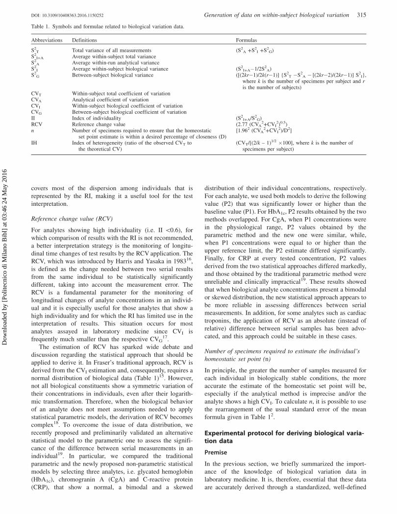
Identifying outliers
For the biological variation estimate of the serum immunoglobulin free kand � light chains (FLC) and k/� FLC ratio calculation, we collected fiveblood specimens from each of 21 enrolled volunteers and each samplewas measured in duplicate80. In Tables A1–A3, we report, as an example,the calculations for outlier identification performed for k FLC withCochran’s statistical test applied to duplicate observations and S2
I+A
values and for Reed’s criterion applied to the average k FLC values ofsubjects, respectively. By consulting the table for Cochran’s testoptimized (for p ¼0.01), one sees that, with a total number of �100values and 2 degrees of freedom, the maximum/sum ratio should be50.142481. Having experimentally obtained a value of 0.154 for this ratioon all observations (Table A1), the highest detected variance(0.21125 mg/L) has to be considered as an outlier and the subjectdisplaying this variance (number 2) eliminated from analyses. Afterremoving the outlier, Cochran’s test was performed again; the maximum/sum ratio was 0.079, which, on the basis of the table for Cochran’s testoptimized, allowed the data to be accepted. Cochran’s test was alsoapplied to S2
I+A values (Table A2). By consulting the table for theCochran’s test optimized (for p ¼0.01), one notes that, with 20 valuesand 4 degrees of freedom, the maximum/sum ratio should be50.265481.Having experimentally obtained a value of 0.28819 for this ratio forS2
I+A values, the maximum variance (3.88997) should be considered asan outlier and the corresponding subject (number 16) should beeliminated from analyses. Cochran’s test was then performed again;the maximum/sum ratio was 0.2611, which allowed the data to beaccepted. Finally, for the application of Reed’s criterion for identificationof outliers among mean values of subjects, the average k FLC values (themean of the five duplicate means) of each individual were considered inascending order (Table A3). To exclude the presence of outliers, thedifferences between the second lowest value (6.20 mg/L) and the lowest(5.88 mg/L) and between the highest value (13.41 mg/L) and the secondhighest (9.85 mg/L) should not be 42.51 mg/L, which is the differencebetween the maximum (13.41 mg/L) and the minimum value (5.88 mg/L), divided by 3. The first difference (0.32 mg/L) was indeed well belowthe limit, but the second one (3.56 mg/L) was much higher. The subjectwith the highest k FLC mean value was then eliminated and Reed’scriterion repeated; this time a difference between the highest value(9.85 mg/L) and the next highest one (9.66 mg/L) of 0.19 mg/L wasobtained, which is lower than one-third of the difference between the twoextreme values (1.32 mg/L). At the end of all steps, after removing all theoutliers, the number of subjects with results usable for the estimate ofbiological variation components for serum k FLC was 1880.
Testing normality of distributions
Reported examples relate to the biological variation studies of threeanalytes with different data distributions.
In studying HbA1c biological variation in a group of 18 subjects19,43,we evaluated the frequency distribution of HbA1c values characterizingthe subject population. The Shapiro–Wilk test accepted the hypothesis ofnormality of the data distribution in the great majority of subjects. The
DOI: 10.3109/10408363.2016.1150252 Generation of data on within-subject biological variation 323
Dow
nloa
ded
by [
Polit
ecni
co d
i Mila
no B
ibl]
at 0
3:46
24
May
201
6

condition of normality was also accepted for the distribution of meanHbA1c values of all subjects and of male and female subgroups.
In studying the biological variation of carbohydrate antigen 125 (CA-125), a biomarker for detecting ovarian cancer recurrence and monitor-ing the therapeutic response, the Shapiro–Wilk test accepted thehypothesis of normality for the distribution of within-subject markervalues for all subjects, while for the distribution of individual mean CA-125 values of enrolled subjects, the normality test failed31. TheKolmogorov–Smirnov test confirmed the skewed distribution.Consequently, a natural log scale transformation was applied beforecalculation. The Shapiro–Wilk test was repeated for the CA-125individual mean values obtained from log-transformed data and thehypothesis of normality was finally accepted. The obtained S2
I, S2G and
overall mean were converted back via inverse natural logarithmicfunction before deriving biological CVs31.
In the study evaluating the biological variation of CRP quotedabove19, the Shapiro–Wilk test failed to accept the hypothesis ofnormality for the distribution of 70% of within-subject values. Therefore,we transformed all data by natural log-scale and repeated the normalitytest. Even after logarithmic transformation, the Shapiro–Wilk test failedto accept the hypothesis of normality for the distribution of 25% ofwithin-subject CRP values. The inability to normalize the distribution ofCRP values prevented the biological variation data derivation for thisanalyte by the traditional protocol based on a parametric calculation ofCVs.
Table A1. Calculations for Cochran’s statistical test for outlier identi-fication applied to the duplicate observations for serum k-free lightchains obtained in a biological variation study (80).
Subject no. Sample (r2� r1)2/2 (mg/L)
1 A 0.00500B 0.00320C 0.00005D 0.02420E 0.00125
2 A 0.21125B 0.00180C 0.08405D 0.00080E 0.00720
3 A 0.00080B 0.00320C 0.01445D 0.00125E 0.03125
4 A 0.00245B 0.00125C 0.06480D 0.00125E 0.03380
5 A 0.04805B 0.00500C 0.08405D 0.04205E 0.00605
6 A 0.00320B 0.00320C 0.04805D 0.01125E 0.01805
7 A 0.01805B 0.00045C 0.00005D 0.00405E 0.02000
8 A 0.00080B 0.00500C 0.00045D 0.00020E 0.00320
9 A 0.00005B 0.00500C 0.00125D 0.01125E 0.00125
10 A 0.00045B 0.02000C 0.00045D 0.00045E 0.03125
11 A 0.00500B 0.00020C 0.04500D 0.01620E 0.00845
12 A 0.02000B 0.00045C 0.00180D 0.00500E 0.02420
13 A 0.02000B 0.00080C 0.00605D 0.00405E 0.00500
14 A 0.00125B 0.00605C 0.05120
(continued )
Table A1. Continued
Subject no. Sample (r2� r1)2/2 (mg/L)
D 0.00020E 0.00405
15 A 0.00720B 0.00020C 0.00045D 0.00405E 0.00000
16 A 0.00080B 0.00000C 0.00980D 0.00020E 0.00500
17 A 0.00980B 0.01445C 0.01280D 0.01620E 0.00245
18 A 0.01620B 0.01620C 0.00125D 0.03125E 0.00005
19 A 0.00245B 0.00005C 0.01280D 0.02000E 0.01125
20 A 0.00045B 0.01125C 0.00605D 0.02205E 0.00845
21 A 0.00605B 0.00045C 0.00005D 0.00845E 0.00005
Total number of variances 105Sum of variances 1.36905 mg/LMaximum variance 0.21125 mg/LMaximum/sum ratio 0.154
r1, replicate 1; r2, replicate 2.
324 F. Braga & M. Panteghini Crit Rev Clin Lab Sci, 2016; 53(5): 313–325
Dow
nloa
ded
by [
Polit
ecni
co d
i Mila
no B
ibl]
at 0
3:46
24
May
201
6
Comparing populations
During an experimental study of biological variation of total copper,ceruloplasmin and copper/ceruloplasmin ratio (Cu:Cp) in serum, meananalyte values and S2
I+A values of male and female subjects werecompared by the unpaired Student’s t-test and the F-test, respectively,using the MedCalc statistical program (MedCalc Software bvba, Ostend,Belgium)82. Mean Cu:Cp values was slightly higher (p¼0.02) in womenthan in men, whereas no sex-dependent difference was found for copperand ceruloplasmin concentrations. However, S2
I+A values of the studiedparameters were not different between the genders; this allowed thederivation of only one CVI value for the whole population.
Assessing the index of heterogeneity
CgA and neuron-specific enolase (NSE) are biomarkers for neuroendo-crine tumors. For the derivation of their biological variation, wecollected five blood specimens from each of 22 apparently healthyvolunteers on the same day of the week, every 2 weeks for 2 months37.With five data points for each subject, the within-subject data arehomogeneous if IH is 50.632. However, the calculated IH (0.768 forCgA and 0.805 for NSE) did not fulfill the homogeneity condition.Consequently, the RCV obtained for CgA and NSE were not directlytransferable to the entire population for the clinical interpretation ofmarker results, but were just suggestive of the extent that changes inresults should reach to indicate the presence of some external sources ofvariation (e.g. disease progression or therapy effectiveness).
Table A2. Calculations for the Cochran’s statistical test foroutlier identification applied to the within-subject vari-ances obtained in a biological variation study of serumk-free light chains (80).
Subject no. S2I+A (mg/L)
1 0.542193 2.508664 0.313165 2.093456 0.171697 0.466938 0.153039 0.13124
10 0.1310011 0.2881712 0.2205813 0.8234614 0.2206315 0.0991416 3.8899717 0.4651418 0.1585719 0.3957920 0.254621 0.17045Total number of variances 20Sum of variances 13.4978 mg/LMaximum variance 3.88997 mg/LMaximum/sum ratio 0.28819
Table A3. Average values for each of theenrolled subjects, displayed in ascendingorder, in a biological variation study ofserum k-free light chains to be used for theapplication of Reed’s criterion (80).
Mean (mg/L)
5.886.206.286.687.207.617.757.948.008.058.448.508.568.669.019.089.669.85
13.41
DOI: 10.3109/10408363.2016.1150252 Generation of data on within-subject biological variation 325
Dow
nloa
ded
by [
Polit
ecni
co d
i Mila
no B
ibl]
at 0
3:46
24
May
201
6