Variational Bayesian causal connectivity analysis for fMRI · convolution with a hemodynamic response function. Due to the employed modeling, it is Due to the employed modeling, it

ORIGINAL RESEARCH ARTICLEpublished: 05 May 2014

doi: 10.3389/fninf.2014.00045

Variational Bayesian causal connectivity analysis for fMRIMartin Luessi1,2*, S. Derin Babacan3, Rafael Molina4, James R. Booth5 and Aggelos K. Katsaggelos2

1 Athinoula A. Martinos Center for Biomedical Imaging, Harvard Medical School, Massachusetts General Hospital, Charlestown, MA, USA2 Department of Electrical Engineering and Computer Science, Northwestern University, Evanston, IL, USA3 Google Inc., Mountain View, CA, USA4 Departamento de Ciencias de la Computación e I.A., Universidad de Granada, Granada, Spain5 Department of Communication Sciences and Disorders, Northwestern University, Evanston, IL, USA

Edited by:

Jesus M. Cortes, Ikerbasque,Biocruces Health Research Institute,Spain

Reviewed by:

Sebastiano Stramaglia, Universitàdegli Studi di Bari, ItalyLotfi Chaari, IRIT-ENSEEIHT, France

*Correspondence:

Martin Luessi, Athinoula A. MartinosCenter for Biomedical Imaging,Harvard Medical School,Massachusetts General Hospital,Building 149, Room 2301, 13thStreet, Charlestown, MA 02129,USAe-mail: [email protected]

The ability to accurately estimate effective connectivity among brain regions fromneuroimaging data could help answering many open questions in neuroscience. Wepropose a method which uses causality to obtain a measure of effective connectivityfrom fMRI data. The method uses a vector autoregressive model for the latent variablesdescribing neuronal activity in combination with a linear observation model based on aconvolution with a hemodynamic response function. Due to the employed modeling, it ispossible to efficiently estimate all latent variables of the model using a variational Bayesianinference algorithm. The computational efficiency of the method enables us to apply it tolarge scale problems with high sampling rates and several hundred regions of interest. Weuse a comprehensive empirical evaluation with synthetic and real fMRI data to evaluatethe performance of our method under various conditions.

Keywords: fMRI, causality, connectivity, variational Bayesian method, Granger causality

1. INTRODUCTIONTraditionally, functional neuroimaging has been used to obtainspatial maps of brain activation, e.g., using functional magneticresonance imaging (fMRI) or positron emission tomography(PET), or to study the spatio-temporal progression of activityusing magneto- or electroencephalography (M/EEG). Due to theincreasing availability of MRI scanners to researchers and dueto their high spatial resolution, the question of how fMRI canbe used to obtain measures of effective connectivity, describingdirected influence and causality in brain networks (Friston, 1994),has recently received significant attention.

An idea that forms the basis of several methods is that causal-ity can be used to infer effective connectivity, i.e., if activity inone region can be used to accurately predict future activity inanother region, it is likely that a directed connection betweenthe regions exists. An exhaustive review of causality based meth-ods for fMRI is beyond the scope of this work; we only providea short introduction and refer to Roebroeck et al. (2011) for arecent review of related methods. Effective connectivity methodsfor fMRI can be divided into two groups. Methods in the firstgroup are referred to as dynamic causal modeling (DCM) methods(Friston et al., 2003). In DCM, the relationship between neu-ronal activity in different regions of interest (ROIs) is describedby bilinear ordinary differential equations (ODEs) and the fMRIobservation process is modeled by a biophysical model based onthe Balloon model (Buxton et al., 1998, 2004). While provid-ing an accurate model of the hemodynamic process underlyingfMRI, the non-linearity of the observation model poses difficul-ties when estimating the latent variables describing the neuronalactivity from the fMRI observations. Due to this, DCM is typicallyused for small numbers of ROIs (less than 10) and DCM methods

typically are confirmatory approaches, i.e., the user provides anumber of different candidate models describing the connectivity,which are then ranked based on an approximation to the modelevidence.

The second class of methods attempts to estimate effective con-nectivity between ROIs from causal interactions that exist in theobserved fMRI time series. In the widely used Wiener–Grangercausality (WGC) measure (Wiener, 1956; Granger, 1969) (referto Bressler and Seth, 2010 for a recent review of related meth-ods), a linear prediction model is employed to predict the futureof one time series using either only its past or its past and thepast of the time series from a different ROI. If the latter leadsto a significantly lower prediction error, the other time series isconsidered to exert a causal influence on the time series beingevaluated, which is indicative of directed connectivity betweenthe underlying ROIs. Related methods estimate the causal con-nectivity between all time series simultaneously by employing avector autoregressive (VAR) model. The magnitudes of the esti-mated VAR coefficients are considered a measure of connectivitybetween regions. In Valdés-Sosa et al. (2005), a first order VARmodel is employed and the connectivity graph is assumed to besparse, i.e., only few regions are connected. The sparsity assump-tion is formalized by using �1-norm regularization of the VARcoefficients. It has been shown in Haufe et al. (2008) that theuse of higher order VAR models in combination with �1�2-norm(group-lasso) (Yuan and Lin, 2006; Meier et al., 2008) regulariza-tion of the VAR coefficients across lags leads to a more accurateestimation of the connectivity structure.

There are two main concerns when estimating effective con-nectivity from causal relations in the observed fMRI time series.First, the processing times at the neuronal level are in the order of

Frontiers in Neuroinformatics www.frontiersin.org May 2014 | Volume 8 | Article 45 | 1

NEUROINFORMATICS

http://www.frontiersin.org/Neuroinformatics/editorialboard



http://www.frontiersin.org/Neuroinformatics/about

http://www.frontiersin.org/Neuroinformatics

http://www.frontiersin.org/journal/10.3389/fninf.2014.00045/abstract

http://community.frontiersin.org/people/u/54415



mailto:[email protected]

mailto:[email protected]


http://www.frontiersin.org

http://www.frontiersin.org/Neuroinformatics/archive

Luessi et al. Variational Bayesian causal connectivity analysis

milliseconds, which is several orders of magnitude shorter thanthe sampling interval (time to repeat, TR) of the MRI scanner.Second, fMRI measures neuronal activity indirectly through theso-called blood oxygen level dependent (BOLD) contrast (Ogawaet al., 1990; Frahm et al., 1992), which depends on slow hemo-dynamic processes. The observation process can be modeled asa convolution of the time series describing the neuronal activ-ity with a hemodynamic response function (HRF). As there isvariability in the shape of the HRF among brain regions and indi-viduals (Handwerker et al., 2004) and the sampling rate of theMRI scanner is low, detecting effective connectivity from causalinteractions that exist in the observed fMRI data is a challeng-ing problem. There has recently been some controversy if this isindeed the case. In David et al. (2008), a study using simulta-neous fMRI, EEG, and intra-cerebral EEG recordings from ratswas performed and it was found that the performance of WGCfor fMRI is indeed poor, unless the fMRI time series of eachregion is first deconvolved with the measured HRF of the sameregion. Using simulations with synthetic fMRI data generatedusing the biophysical model underlying DCM, it was also foundin Smith et al. (2011) that WGC methods perform poorly relativeto the other evaluated connectivity methods. On the other hand,another recent study (Deshpande et al., 2010) found that WGCmethods provide a high accuracy for the detection of causal inter-actions at the neuronal level with interaction lengths of hundredsof milliseconds, i.e., much shorter than the TR of the MRI scan-ner, even when HRF variations are present. The minor influenceof HRF variations may be explained by the property that typicalHRF variations do not simply correspond to temporal shifts of anHRF with the same shape, which would change the causality ofinteractions present in the fMRI data. Instead, as pointed out inDeshpande et al. (2010), the HRF variability among brain regionsis mostly apparent in the shape of the peak of the HRF and thetime-to-peak (Handwerker et al., 2004), which may explain whycausal interactions at the neuronal level can still be present afterconvolution with varying HRFs. This is in agreement with recentresults. It has been shown that WGC is invariant to filtering withinvertible filters (Barnett and Seth, 2011) and in Seth et al. (2013)simulations were performed that confirm that the invariance typi-cally holds for HRF convolution. However, at the same time it wasfound that WGC can be severely confounded when HRF convo-lution is combined with downsampling and measurement noiseis added to the data.

Several methods have been proposed that account for HRFvariability when analyzing WGC from fMRI data. In David et al.(2008) a noise-regularized HRF deconvolution was employed.and in Smith et al. (2010) a switching linear dynamical system(SLDS) model is proposed to describe the interaction betweenlatent variables representing the neuronal activity together witha linear observation model based on a convolution with a(unknown) HRF for each region. The method employs a Bayesianformulation and obtains estimates of the latent variables using themaximum-likelihood approach. In contrast to WGC methods,the SLDS model can also account for modulatory inputs whichchange the effective connectivity of the network and introducenon-stationarity in the observed fMRI data. The method in Smithet al. (2010) can be seen as a convergence of DCM methods and

WGC-type methods (Roebroeck et al., 2011). A similar method isproposed in Ryali et al. (2011), which can be considered a multi-variate extension of methods which perform deconvolution of theneuronal activity for a single fMRI time series (Penny et al., 2005;Makni et al., 2008). Joint estimation of the HRF and detection ofneuronal activity is also an important problem for event-relatedfMRI, we refer to Cassidy et al. (2012) and Chaari et al. (2013) forrecently proposed methods addressing this problem.

In this paper, we propose a causal connectivity method forfMRI which employs a VAR model of arbitrary order for the timeseries of neuronal activity in combination with a linear hemody-namic convolution model for the fMRI observation process. Weuse a Bayesian formulation of the problem and draw inferencebased on an approximation to the posterior distribution whichwe obtain using the variational Bayesian (VB) method (Jordanet al., 1999; Attias, 2000). In contrast to previous methods (Smithet al., 2010; Ryali et al., 2011), our method is designed to be com-putationally efficient, enabling application to large scale problemswith large numbers of regions and high temporal sampling rates.Computational efficiency is achieved by the introduction of anapproximation to the neuronal time series in the Bayesian mod-eling. When drawing inference, introducing this approximationhas the effect that the hemodynamic deconvolution can be sep-arated from the estimation of the neuronal time series, leadingto a reduction of the state-space dimension of the variationalKalman smoother (Beal and Ghahramani, 2001; Ghahramaniand Beal, 2001), which forms a part of the VB inference algo-rithm. The lower state-space dimension drastically reduces theprocessing and memory requirements. Another key difference toprevious Bayesian methods is that we assume that the VAR coef-ficient matrices are sparse and that the coefficient matrices atdifferent lags have non-zero entries at mostly the same locations,i.e., the matrices have similar sparsity profiles. In Haufe et al.(2008) this assumption is formalized using an �1�2-norm regu-larization term for the VAR coefficient matrices. In our work, weemploy Gaussian priors with shared precision hyperparametersfor the VAR coefficient matrices, which is a Bayesian alternativeto �1�2-norm regularization and results in a higher estimationperformance of the method.

Our results show that the proposed method offers a higherdetection performance than WGC when the number of nodes islarge or when the SNR is low. In addition, our method is lessaffected when the VAR model order assumed in the method ishigher than the order present in the data. We also perform simu-lations using a modified version of our method, which is similarto the method in Ryali et al. (2011), and show that the approx-imation to the neuronal time series used in our method has anegligible effect on the estimation performance while allowingthe application of the proposed method to large problems withhundreds of ROIs. We perform an extensive series of simulationswhere we vary both the downsampling ratio and the neuronaldelay. The results show that the proposed method offers somebenefits over WGC, especially in low SNR situations and whenHRF variations are present. However, both the proposed methodand WGC can at times detect a causal influence with the oppo-site direction of the true influence, which is a known problem forWGC methods (David et al., 2008; Deshpande et al., 2010; Seth






et al., 2013). Finally, we apply the proposed method to resting-state fMRI data from the Human Connectome Project (Van Essenet al., 2012), where it successfully detects connections betweenregions that belong to known resting-state networks.

This paper is outlined as follows. First, we introduce a hierar-chical Bayesian formulation for the generative model underlyingthe fMRI connectivity estimation problem. Next, we present theBayesian inference scheme which estimates the latent variables ofthe model using a variational approximation to the posterior dis-tribution. We then perform extensive simulations with syntheticfMRI data. Finally, we apply the method to real fMRI data andconclude the paper.

1.1. NOTATIONWe use the following notation throughout this work: Matricesare denoted by uppercase bold letters, e.g., A, while vectors aredenoted by lowercase bold letters, e.g., a. The element at the i-throw and j-th column of matrix A is denoted by aij, while ai· and a·jdenote column vectors with the elements from the i-th row andthe j-th column of A, respectively. The operator diag (A) extractsthe main diagonal of A as a column vector, whereas Diag (a) isa diagonal matrix with a as its diagonal. The operator vec (A)

vectorizes A by stacking its columns, tr (A) denotes the trace ofmatrix A, and ⊗ denotes the Kronecker product. The identitymatrix of size N × N is denoted by IN . Similarly, 0N and 0N×M

denote N × N and N × M all-zero matrices, respectively.

2. BAYESIAN MODELINGThe goal of this work is to infer effective connectivity implied bythe causal relations between N time series of neuronal activityfrom N different regions in the brain. To this end, we employ avector autoregressive (VAR) model of order P to model the timeseries as follows

s (t) =P∑

p = 1

A(p)s(t − p

) + η (t) , (1)

where s (t) ∈ RN denotes the neuronal activity of all regions at

time t, A(p) ∈ RN×N is a matrix with VAR coefficients for lag p,

and η (t) ∼ N (0, �−1

)denotes the innovation. In this model,

the activity at any time point is predicted from the activity at Pprevious time points. More specifically, the activity of the i-thtime series at time t, denoted by si (t), is predicted from the past

of the j-th time series using the coefficients {a(p)ij }P

p = 1. Hence, ifany of these coefficients is significantly larger than zero, we canconclude that the j-th time series exerts a causal influence on thei-th time series, implying connectivity between the regions. Thisis the idea underlying Wiener–Granger causality (Wiener, 1956;Granger, 1969) and related methods using vector autoregressivemodels (Valdés-Sosa et al., 2005; Haufe et al., 2008).

We can now introduce an embedding process (Weigend andGershenfeld, 1994; Penny et al., 2005) x (t) defined by

x (t) =[

s (t)T s (t − 1)T . . . s (t − P + 1)T]T

, (2)

which allows us to express (Equation (1)) by a first order VARmodel as follows

x (t) = Ax (t − 1) + η (t) , (3)

where A ∈ RPN×PN is given by

A =

⎡⎢⎢⎢⎢⎢⎢⎣A(1) A(2) · · · A(P−1) A(P)

IN 0N · · · 0N 0N

0N IN · · · 0N 0N...

.... . .

......

0N 0N · · · IN 0N

⎤⎥⎥⎥⎥⎥⎥⎦ . (4)

The innovation η (t) is Gaussian η (t) ∼ N (0, Q), where thecovariance matrix Q is all zero, except for the first N rows andcolumns, which are given by �−1. For the remainder of this paper,we present the modeling and inference with respect to the timeseries x (t). If access to the neuronal time series s (t) is required,it can easily be extracted from x (t) (it simply corresponds to thefirst N elements of x (t)).

2.1. OBSERVATION MODELBefore introducing the observation model, note that we canobtain a noisy version of the neuronal time series from theembedding process x (t) as follows

z (t) = Bx (t) + κ (t) , (5)

where B = [IN 0N×(P − 1)N

]and κ (t) ∼ N (

0, ϑ−1I), where ϑ

is the precision parameter. Clearly, by using very large valuesfor ϑ , the time series z (t) approaches s (t). The introduction ofthis Gaussian approximation to the neuronal time series greatlyimproves the computational efficiency of the proposed method,as it separates the VAR model for the neuronal time series fromthe hemodynamic observation model. This separation leads to areduction of the state-space dimension of the Kalman smooth-ing algorithm, which forms part of the inference procedure,and therefore to greatly reduced memory requirements. In addi-tion, using the approximation allows us to perform parts of theestimation in the frequency domain, which is computationallyadvantageous due to the efficiency of the fast Fourier transform.The computational advantages of the proposed method will bediscussed in detail in the next section.

To model the fMRI observation process, we follow the stan-dard assumption underlying the general linear model (Fristonet al., 1995), and express the fMRI observation of the i-th regionas follows

yi (t) = hi (t) ∗ zi (t) + εi (t)

=L∑

k = 1

hi (k) zi (t − k + 1) + εi (t) , (6)

where ∗ denotes the convolution operation, hi (t) is the hemody-namic response function (HRF) of length L for the i-th region,and εi (t) denotes observation noise. Notice that we can arrange






the HRF hi (t) into a T × T convolution matrix Hi, which allowsus to write (Equation (6)) as

yi = Hizi + εi, (7)

where the T × 1 vectors yi, zi, and εi are the fMRI observation,the approximation to the neuronal signal, and the observationnoise, for the i-th region, respectively.

2.2. VAR COEFFICIENT PRIOR MODELWe proceed by defining priors for the VAR coefficient matrices{

A(p)}P

p = 1. For a network consisting of a large number of regions,

it can generally be assumed that the connectivity is sparse, i.e.,the VAR coefficient matrices contain a small number of non-zerocoefficients. In the context of inferring causal connectivity, thisidea has been used in Valdés-Sosa et al. (2005), where a first orderVAR model with �1-norm regularization for the VAR coefficientsis used to obtain a sparse solution. For higher order VAR models,

it is intuitive to assume that if the VAR coefficient a(p1)ij modeling

the connectivity from region j to region i and lag p1 is non-zero,it is likely that also other VAR coefficients for the same con-

nection but different lags, i.e., a(p2)ij , p2 �= p1, are also non-zero.

Together with the sparsity assumption, this leads to VAR coef-ficient matrices with similar sparsity profiles, i.e., the coefficientmatrices at different time lags have non-zero entries at mostly thesame locations. In Haufe et al. (2008) this idea is formalized byusing �1�2-norm (group lasso) (Yuan and Lin, 2006; Meier et al.,2008) regularization for the VAR coefficients across different lags,resulting in an improved estimation performance in comparisonto methods that use alternative forms of regularization, such as,�1-norm or ridge regression.

We incorporate the group sparsity assumption using Gaussianpriors with shared precision hyperparameters across differentlags. More specifically, we use

p(

A(p)|�)

=N∏

i = 1

N∏j = 1

N(

a(p)ij | 0, γ −1

ij

)p ∈ {1, . . . , P}, (8)

with Jeffreys hyperpriors to the precision hyperparameters

p (�) ∝N∏

i = 1

N∏j = 1

(γij

)−1. (9)

During estimation, most of the precision hyperparameters in� will assume very large values, hence effectively forcing thecorresponding VAR coefficients to zero. This formulation is anadaptation of sparse Bayesian learning (also known as automaticrelevance determination, ARD) (Tipping, 2001) to the problemof VAR coefficient estimation and can be considered a Bayesianalternative to a deterministic �1�2-norm regularization term.Formulations where shared precision hyperparameters are usedto enforce group sparsity have recently been proposed for applica-tions such as simultaneous sparse approximation (Wipf and Rao,2007), where shared precision parameters are used to obtain solu-tions with similar sparsity profiles across multiple time points.

Recently, shared hyperparameters were used to model the low-rank structure of the latent matrix in matrix estimation (Babacanet al., 2012).

2.3. INNOVATION AND NOISE PRIOR MODELSTo complete the description of the Bayesian model, we definepriors for the innovation process and the observation noise inEquations (1) and (6), respectively. We assume that the inno-vations are independent and identically distributed (i.i.d.) zero-mean Gaussian for each time point, i.e., η (t) ∼ N (

0, �−1)

andε (t) ∼ N (0, R). It has to be expected that the linear predic-tion model used in the proposed method cannot fully explain therelationship between the neuronal time series in different ROIs.Hence, the precision matrix � can contain some non-zero off-diagonal elements. We model this using a Wishart prior for theprecision matrix

p (�) = W (�|ν0, W0) , (10)

where ν0 and W0 are deterministic parameters. By using a diag-onal matrix for W0, we obtain a prior modeling that encourages� to be diagonal, which is the structure usually assumed in VARmodels. Another reason for chosing this prior modeling is thatthe Wishart distribution is the conjugate prior for the preci-sion matrix of the Gaussian distribution, which simplifies theinference procedure.

For the observation noise, we assume that the noise in differ-ent regions is uncorrelated and use diagonal covariance matricesgiven by R = Diag (β)−1, where β is a precision hyperparametervector of length N. We use conjugate gamma hyperpriors for theprecisions as follows

p (β) =N∏

i = 1

�(βi|a0

β, b0β

), (11)

where the gamma distribution with shape parameter a andinverse scale parameter b is given by

� (ξ |a, b) = ba

� (a)ξ a − 1 exp (−bξ) . (12)

We usually have some information about the fMRI observationnoise and can use this knowledge to set the parameters a0

β and b0β .

The setting of the deterministic parameters will be discussed inmore detail in the next section.

2.4. GLOBAL MODELINGBy combining the probability distribution describing the VARmodel, the fMRI observation model, and the prior model, weobtain a joint distribution over all latent variables and knownquantities as

p(, {y(t)}T

t = 1

)=

(N∏

i = 1

p(

yi|zi, Hi, βi))(

T∏t = 1

p (z(t)|x(t), ϑ)

)

×(

T∏t = 1

p(

x(t)|x(t − 1) , {A(p)}Pp = 1, �

))






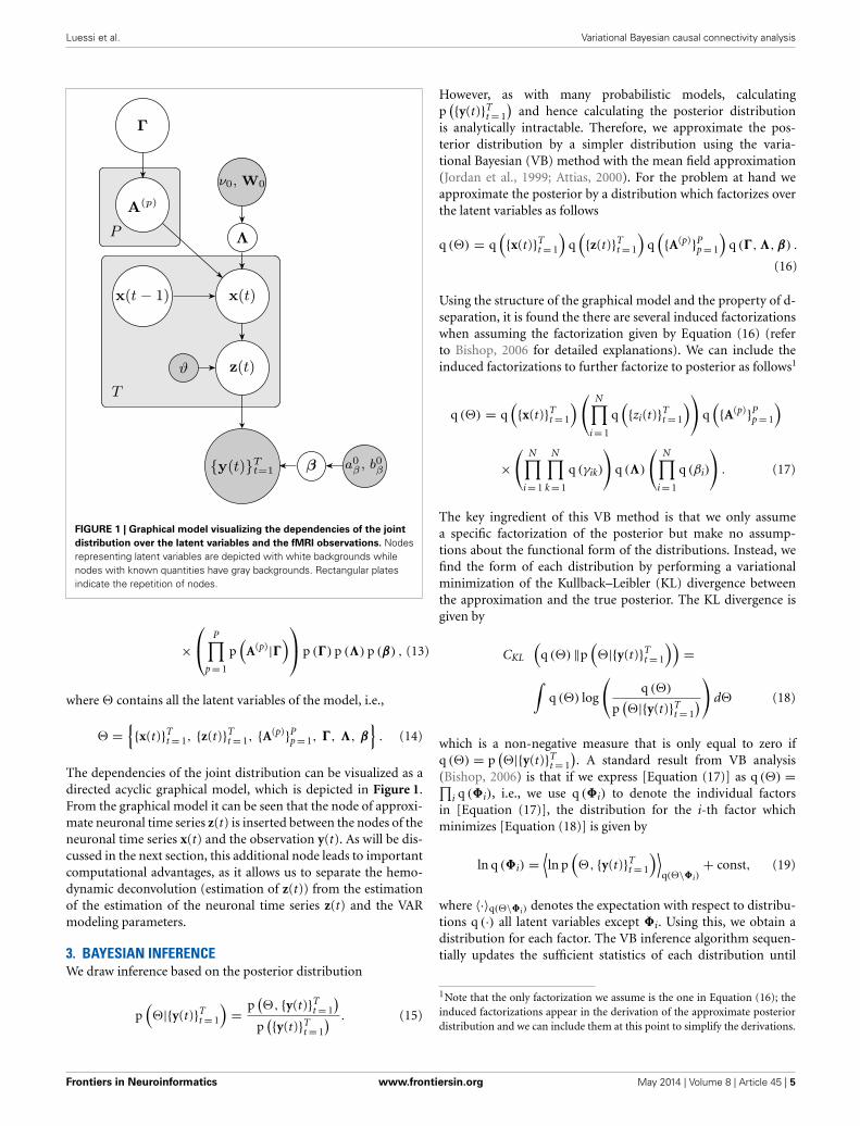
FIGURE 1 | Graphical model visualizing the dependencies of the joint

distribution over the latent variables and the fMRI observations. Nodesrepresenting latent variables are depicted with white backgrounds whilenodes with known quantities have gray backgrounds. Rectangular platesindicate the repetition of nodes.

×⎛⎝ P∏

p = 1

p(

A(p)|�)⎞⎠ p (�) p (�) p (β) , (13)

where contains all the latent variables of the model, i.e.,

={{x(t)}T

t = 1, {z(t)}Tt = 1, {A(p)}P

p = 1, �, �, β}

. (14)

The dependencies of the joint distribution can be visualized as adirected acyclic graphical model, which is depicted in Figure 1.From the graphical model it can be seen that the node of approxi-mate neuronal time series z(t) is inserted between the nodes of theneuronal time series x(t) and the observation y(t). As will be dis-cussed in the next section, this additional node leads to importantcomputational advantages, as it allows us to separate the hemo-dynamic deconvolution (estimation of z(t)) from the estimationof the estimation of the neuronal time series z(t) and the VARmodeling parameters.

3. BAYESIAN INFERENCEWe draw inference based on the posterior distribution

p(|{y(t)}T

t = 1

)= p

(, {y(t)}T

t = 1

)p

({y(t)}Tt = 1

) . (15)

However, as with many probabilistic models, calculatingp

({y(t)}Tt = 1

)and hence calculating the posterior distribution

is analytically intractable. Therefore, we approximate the pos-terior distribution by a simpler distribution using the varia-tional Bayesian (VB) method with the mean field approximation(Jordan et al., 1999; Attias, 2000). For the problem at hand weapproximate the posterior by a distribution which factorizes overthe latent variables as follows

q () = q({x(t)}T

t = 1

)q({z(t)}T

t = 1

)q({A(p)}P

p = 1

)q (�, �, β) .

(16)

Using the structure of the graphical model and the property of d-separation, it is found the there are several induced factorizationswhen assuming the factorization given by Equation (16) (referto Bishop, 2006 for detailed explanations). We can include theinduced factorizations to further factorize to posterior as follows1

q () = q({x(t)}T

t = 1

)(N∏

i = 1

q({zi(t)}T

t = 1

))q({A(p)}P

p = 1

)

×(

N∏i = 1

N∏k = 1

q (γik)

)q (�)

(N∏

i = 1

q (βi)

). (17)

The key ingredient of this VB method is that we only assumea specific factorization of the posterior but make no assump-tions about the functional form of the distributions. Instead, wefind the form of each distribution by performing a variationalminimization of the Kullback–Leibler (KL) divergence betweenthe approximation and the true posterior. The KL divergence isgiven by

CKL

(q () ‖p

(|{y(t)}T

t = 1

))=∫

q () log

(q ()

p(|{y(t)}T

t = 1

))d (18)

which is a non-negative measure that is only equal to zero ifq () = p

(|{y(t)}T

t = 1

). A standard result from VB analysis

(Bishop, 2006) is that if we express [Equation (17)] as q () =∏i q (�i), i.e., we use q (�i) to denote the individual factors

in [Equation (17)], the distribution for the i-th factor whichminimizes [Equation (18)] is given by

ln q (�i) =⟨ln p

(, {y(t)}T

t = 1

)⟩q(\�i)

+ const, (19)

where 〈·〉q(\�i) denotes the expectation with respect to distribu-tions q (·) all latent variables except �i. Using this, we obtain adistribution for each factor. The VB inference algorithm sequen-tially updates the sufficient statistics of each distribution until

1Note that the only factorization we assume is the one in Equation (16); theinduced factorizations appear in the derivation of the approximate posteriordistribution and we can include them at this point to simplify the derivations.






convergence. Below we show the functional form of the varia-tional posterior distribution for each latent variable. Due to spaceconstraints, the derivations are not shown here and we refer toLuessi (2011) for more details.

Using Equation (19), the distribution for the neuronal timeseries q

({x(t)}Tt = 1

)is obtained from

ln q({x(t)}T

t = 1

)=

⟨ln

T∏t = 1

p(

x(t)|x(t − 1) , {A(p)}Pp = 1, �

)×p (z(t)|x(t),ϑ)

⟩q({z(t)}T

t = 1

)q({A(p)}P

p = 1

)q(�,�,β)

+ const,

(20)

where all terms not depending on {x(t)}Tt = 1 have been absorbed

into the additive normalization constant. Due to the conjugacy ofthe priors, q

({x(t)}Tt = 1

)is a multivariate Gaussian distribution

with dimension TPN. However, this distribution has a compli-cated form and cannot be further factorized, which makes a directcalculation of the sufficient statistics computationally infeasible.Note that this complication is not due to the introduction of z(t);it is also present in methods which do not employ the approx-imate time series z(t). Fortunately, Equation (20) has a similarform as an equation encountered in the variational Kalmansmoothing algorithm (Beal and Ghahramani, 2001; Ghahramaniand Beal, 2001), with the only difference that instead of using theobservations we use the expectation of z(t) under q

({z(t)}Tt = 1

).

The variational Kalman smoothing algorithm recursively esti-mates q (x(t)) = N (

x(t)|μt, t)

using a forward and a backwardrecursion. It is important to point out that we do not introducean additional factorization of q

({x(t)}Tt = 1

)over time points, as

for example done in Makni et al. (2008), which has been shownto result in an inaccurate approximation to the posterior distri-bution for large T (Wang and Titterington, 2004). Instead, thevariational Kalman smoothing algorithm provides an efficientway for estimating q

({x(t)}Tt = 1

)without assuming a factorization

over time points.In our implementation we ignore the contribution from the

covariances in the quadratic terms of {A(p)}Pp = 1, i.e., we assume⟨(

A(p))T (

A(p))⟩ = ⟨

A(p)⟩T ⟨

A(p)⟩. This assumption is also made in

Ryali et al. (2011) and can be expected to have only a minorinfluence on the performance of the proposed method. The mainreason for using this approximation is that we do not need

to calculate and store the covariance matrix of q({A(p)}P

p = 1

),

which greatly reduces the computational requirements of themethod. Another effect of using this approximation is that therecursive inference algorithm becomes similar to the standardKalman smoothing algorithm, also known as the Rauch-Tung-Striebel smoother (Rauch et al., 1965). For the forward pass,we use the initial conditions μ0

0 = 0, 00 = I and calculate for

t = 1, 2, . . . , T the following

μt−1t = ⟨

A⟩μt − 1

t − 1 (21)

t − 1t = ⟨

A⟩t − 1

t − 1

⟨A⟩T + 〈Q〉 (22)

μtt = μt − 1

t + Kt(〈z (t)〉 − Bμt − 1

t

)(23)

tt = t − 1

t − KtBt − 1t , (24)

where the Kalman gain is given by

Kt = t − 1t BT

(Bt − 1

t BT + ϑ−1IN

)−1. (25)

After the forward pass, the final estimate for the last time pointhas been obtained, i.e., we have μT = μT

T and T = TT . For the

remaining time points we execute a backward pass and calcu-late the sufficient statistics of q (x(t)) for t = t − 1, t − 2, . . . , 1as follows

μt = μtt + Jt

(μt + 1 − ⟨

A⟩μt

t

), (26)

t = tt + Jt

(t

t − tt + 1

)JT

t , (27)

where

Jt = tt

⟨A⟩T (

tt+1

)−1. (28)

As the posterior distributions of individual time points arenot independent, i.e., q

({x(t)}Tt = 1

) �= ∏Tt = 1 q (x(t)), cross-

time expectations contain a cross-time covariance t,t − 1, i.e.,⟨x(t)x(t − 1)T

⟩ = μtμTt − 1 + t,t − 1. Such cross-time covariance

terms are computed as follows (see Ghahramani and Hinton,1996)

t,t − 1 = tJTt − 1 + Jt

(t + 1,t − ⟨

A⟩t

t

)JT

t − 1. (29)

The posterior distribution of the approximate time series for thei-th region q

({zi(t)}Tt = 1

)is found to be a Gaussian, that is,

q({zi(t)}T

t = 1

)= N

(zi| 〈zi〉 , i

z

), (30)

with parameters

〈zi〉 = iz

(〈βi〉 HT

i yi + ϑ 〈xi〉)

, (31)

zi =

(〈βi〉 HT

i Hi + ϑIT

)−1. (32)

The distribution for the VAR coefficients a =vec

([A(1) A(2) · · · A(P)

])is also Gaussian, the mean and

covariance matrix are given by

〈a〉 = avec

(〈�〉

[T∑

t = 1

(μt

)1:N μT

t − 1 + (t,t − 1

)1:N,:

])(33)

−1a = P1 ⊗ 〈�〉 + Diag (IP ⊗ vec (〈�〉)) , (34)

where the matrix P1 is given by

P1 =T∑

t = 1

⟨x(t − 1)x(t − 1)T

⟩=

T∑t = 1

μt − 1μTt − 1 + t − 1.(35)






Notice that the size of −1a is N2P × N2P. Hence, for large N

performing a direct inversion is computationally very demand-ing and potentially numerically inaccurate. Moreover, storing thematrix requires large amounts of memory. Instead of directlyinverting the matrix, we use a conjugate gradient (CG) algorithmto solve

−1a 〈a〉 = vec

(〈�〉

[T∑

t = 1

(μt

)1:N μT

t − 1 + (t,t − 1

)1:N,:

]),(36)

for 〈a〉, which is possible since −1a is symmetric positive definite.

The CG algorithm only needs to compute matrix-vector productsof the form −1

a p. From the structure of −1a , one can see that the

multiplication of the diagonal matrix on the right side is simplythe element-wise product of the diagonal of Diag (IP ⊗ vec (〈�〉))and p, which can be computed efficiently. Similarly, (P1 ⊗ 〈�〉) pcan be computed efficiently without computing the Kroneckerproduct (Fernandes et al., 1998).

Note that computation of the gamma hyperparametersrequires access to the diagonal elements of a. Since we donot explicitly compute a, we approximate the diagonal by

Diag (a) ≈ Diag(diag

(−1

a

))−1. We performed experiments

with small N where we calculated a directly using a matrixinversion. We found that using the CG algorithm with an approxi-mation to the diagonal of the covariance matrix results in virtuallythe same estimation performance for the proposed method, whilebeing much faster and more memory efficient.

The posterior for the noise precision � is Wishart distributedwith q (�) = W (�|ν, W) where the parameters are given by

ν = T + ν0, (37)

W−1 = 〈P2〉 + W−10 . (38)

The expectation 〈P2〉 is given by

〈P2〉 =T∑

t = 1

((μt

)1:N − ⟨

A⟩μt − 1

) ((μt

)1:N − ⟨

A⟩μt − 1

)T

− (t,t − 1

)1:N, :

⟨A⟩ − ⟨

A⟩T (

t,t − 1)T

1:N, :

+ (t)1:N,1:N + ⟨A⟩t − 1

⟨A⟩T

, (39)

where A = [A(1) A(2) · · · A(P)

], (t)1:N,1:N is the top left N × N

block of t , and(t,t − 1

)1:N, : are the first N rows of t,t − 1.

The mean of the Wishart distribution is given by 〈�〉 = νW,which is the value used in the other distribution updates in theVB algorithm.

The distribution for the VAR precision hyperparameter q(γij

)is found to be a gamma distribution with shape and inverse scaleparameters

ai,jγ = P

2, b

i,jγ = 1

2

P∑p = 1

(⟨a

(p)ij

⟩2 + a(p)ij

), (40)

where a(p)ij is the variance of a

(p)ij , which we obtain from the

approximation to the diagonal of a. Similarly, the posteriorfor the observation noise precision is a gamma distribution withthe following shape parameter ai

β = T/2 + a0β and inverse scale

parameter

biβ = 1

2

[yT

i yi − 2yTi Hi 〈zi〉 + 〈zi〉T HT

i Hi 〈zi〉 + tr(

HTi Hi

zi

)]+ b0

β .

(41)

3.1. SELECTION OF DETERMINISTIC PARAMETERSThe proposed method has several deterministic parameters whichhave to be specified by the user, namely, the observation noiseprecision parameters {a0

β, b0β}, the VAR model noise parameters

{ν0, W0}, and the neuronal approximation precision ϑ . Typically,an estimate of the noise variance σ 2 present in the data is availableto the user. If this case, a reasonable setting of the observa-tion noise precision parameters is a0

β = c, b0β = cσ 2, where c is

a constant related to the confidence in our initial noise estimate.For very small values of c, the observation noise precision willbe estimated solely by the algorithm, while a high value forcesthe estimated noise precision to the value specified by the user.Unless otherwise noted, we assume throughout this work that anestimate of the noise variance is available and use c = 109.

On the other hand, the user typically does not have precise apriori knowledge of the AR innovation precision. In this case, oneoption is to use ν0 = 0, W−1

0 = 0, which is equivalent to an non-informative Jeffreys prior for the AR innovation precision matrix.However, we observed that 〈�〉 can attain values that are too largewhen a non-informative prior is used. This behavior is caused bythe fact that the convolution with the HRF acts as a low-pass filterand it is generally not possible to perfectly recover the high fre-quency content of the neuronal signal, causing an over-estimationof the AR innovation precision. We found that using ν0 = 1 andW0 = 10−3I, prevents 〈�〉 from attaining too large values andwe use this setting in all experiments presented in this work.Naturally, the parameter setting depends on the scale of the fMRIobservation. Throughout this work, we rescale the fMRI obser-vation to have an RMS value of 6.0, where the root-mean-square

(RMS) value is calculated as RMS =√(∑T

t = 1 ‖y (t) ‖22

)/ (NT).

Note that the choice of RMS = 6.0 is arbitrary, i.e., different val-ues could be used but then other deterministic parameters wouldhave to be modified accordingly. Finally, the approximation preci-sion parameter ϑ plays an important role. In Equation (32) it actssimilarly to a regularization parameter while having the role of theobservation noise precision in the variational Kalman smoother.We heuristically found that using a value that is higher than theobservation noise precision works well and we use ϑ = 10/σ 2

throughout this work.

3.2. COMPUTATIONAL ADVANTAGES OF THE PROPOSED APPROACHTo conclude this section, we highlight some important advan-tages in terms of computational requirements of the proposedmethod over previous approaches. The advantages of the pro-posed method are directly related to the introduction of theapproximate time series z(t).






The first advantage is due to the separation of the model of theneuronal time series from the hemodynamic convolution model,which leads to a reduced state-space dimension of the Kalmansmoothing algorithm. More specifically, in Smith et al. (2010);Ryali et al. (2011), the observation process is modeled as

y(t) = Hx(t) + ε (t) , (42)

where H ∈ RN×NL is a matrix that contains the HRFs of allregions. This modeling requires that x(t) is an embedding pro-cess over L time points, i.e., the dimension of x(t) is D = NL, asopposed to D = NP in our method. The higher dimension leadsto excessive memory requirements as the state-space dimensionof the Kalman smoothing algorithm is increased and a total of2T covariance and cross-time covariance matrices of size D × Dneed to be stored in memory. As an example, assuming doubleprecision floating point arithmetic and P = 2, L = 20, N = 100,T = 1000, the methods in Smith et al. (2010) and Ryali et al.(2011) require approximately 60 GB of memory to store thecovariance matrices, whereas the proposed method only requiresapproximately 600 MB. The large memory consumption and thehigher dimension of the required matrix inversions is the rea-son why previous methods become computationally infeasible forlarge scale problems where N ≈ 100 and T ≈ 1000. The problemis even more severe for low TR values, since the HRF typicallyhas a length of about 30 s and a higher sampling rate meansmore samples are needed to represent the HRF, thus increasingthe value of L.

The second advantage due to introduction of z(t) is that theapproximate posterior of z(t) factorizes over ROIs and we canupdate the posterior distribution q

({zi(t)}Tt = 1

)for each region

separately using Equations (31, 32). For large numbers of timepoints this computation can still be expensive as the inversion ofa T × T matrix is required. However, notice that if we assumethat the convolution with hi is circular, the matrix Hi becomescirculant. Circulant matrices can be diagonalized by the discreteFourier transform (see, e.g., Moon and Stirling, 2000). Hence,it is possible to perform the calculation of 〈zi〉 in the frequencydomain. In our implementation we use a fast Fourier transform(FFT) algorithm with zero-padding such that the circular con-volution corresponds to a linear convolution. The resulting timecomplexity is O

(T log T

), compared to O

(T3

)when a direct

matrix inversion is used. Moreover, notice that zi is circulant as

well, which allows us to reduce the computational and memoryrequirements by only calculating and storing the first row of z

i(all other rows can be obtained by circular shifts of the first row).

4. EMPIRICAL EVALUATION WITH SIMULATED DATAIn this section, we evaluate the performance of the proposedmethod using a number of different simulation scenarios. Inall simulations, the proposed method is denoted by “VBCCA”(Variational Bayesian Causal Connectivity Analysis). For compar-ison purposes we include the conditional WGC analysis methodimplemented in the “Granger Causal Connectivity Analysis(GCCA) toolbox” (Seth, 2010), which we denote by “WGCA”(Wiener–Granger Causality Analysis). Note that we use WGCAfor comparison as it is a widely used method with publicly

available implementations. More recent methods, such as themethods from , Smith et al. (2010), Marinazzo et al. (2011) andRyali et al. (2011) may offer a higher estimation performance thanWGCA. However, their high computational complexity makes itdifficult to apply them to large-scale problems, which is the situa-tion where our method clearly outperforms WGCA. Nevertheless,we include a comparison with a modified version of our method,which does not use an approximation to the neuronal time seriesand is therefore more similar to the method from Ryali et al.(2011), and show that for small networks our method providesa comparable estimation performance.

4.1. QUALITY METRICSWe use two objective metrics to evaluate the performance of themethods. The first metric serves to quantify the performance interms of correctly detecting the presence of a connection betweenregions, without taking the direction of the causal influence intoaccount. In order to do so, we calculate the area under the receiveroperating characteristic (ROC) curve, which is commonly used insignal detection theory and has also previously been used to eval-uate connectivity methods (Valdés-Sosa et al., 2005; Haufe et al.,2008). In the following we give a short explanation of the ROCcurve and refer the reader to Fawcett (2006) for a more detailedintroduction. The ROC curve is generated by applying thresholdsto the estimated connectivity scores. The resulting binary masksare compared with the ground truth, resulting in a number oftrue positives (TP) and false positives (FP). From the TP and FPnumbers, we can calculate the true positive rate (TPR) and falsepositive rate (FPR) as follows

TPR = TP

P, FPR = FP

N, (43)

where P and N are the total number of positives and negatives,respectively. For each threshold, we obtain a (FPR, TPR) point inthe ROC space. By applying all possible thresholds, we can con-struct the ROC curve which allows us to compute the area underthe curve (AUC). The AUC is the metric used here to evaluate theconnection detection performance. The value of the AUC is onthe interval [0 1], with 1.0 being perfect detection performancewhile 0.5 is the performance of a random detector, i.e., the AUCshould always be above 0.5 and as close as possible to 1.0. To cal-culate the non-directional connectivity score between nodes i andj from the estimated N × N connectivity matrix, we use the largerof the directional scores, i.e., con(i, j) = con(j, i) = max (cij, cji).For WGCA, the matrix C is the matrix with estimated Grangercausality scores, whereas for the proposed method we calculate C

from the estimated VAR coefficients using cij =√∑P

p = 1

⟨a

(p)ij

⟩.

The AUC provides information on the performance in termsof detecting connections without taking directionality intoaccount. A second metric, denoted by “d-Accuracy” (Smith et al.,2011), is used to evaluate the ability of a method to correctly iden-tify the direction of the connection. The d-Accuracy is calculatedas follows. For true connections (known from the ground truth)we compare the elements cij and cji in the connectivity matrix. Wedecide that the direction was estimated correctly if cij > cji andthe true connection has the direction j → i. By repeating for all






connections, we calculate the overall probability that the direc-tion was estimated correctly, which is the d-Accuracy score. Likethe AUC, the d-Accuracy lies between 0 and 1 with 1.0 indicatingperfect performance and 0.5 being the performance of a randomdirectionality detector.

4.2. NETWORK SIZE AND SNRIn this experiment we evaluate the performance of the pro-posed method for a number of networks of varying sizes and anumber of different signal-to-noise ratios (SNRs). We generateneuronal time series according to Equation (1) where we simu-late connectivity by randomly activating N/2� uni-directionalconnections, for which we generate the VAR coefficients accord-

ing to a(p)ij ∼ N (0, 0.05) ∀ p ∈ {1, . . . , P}, with P = 2. The noise

term is chosen to be Gaussian with unit variance, i.e., η (t) ∼N (0, IN). Using the VAR coefficient matrices we generate a neu-ronal time series s (t) with a total of T = 500 time points. Togenerate the fMRI observations, we convolve the neuronal timeseries of each node with the canonical HRF implemented in SPM8(http://www.fil.ion.ucl.ac.uk/spm/), which has a positive peak at5 s and a smaller negative peak at 15.75 s. The HRF used has atotal length of 30 s assuming a sampling rate of 1 Hz (L = 30).Finally, to generate the noisy fMRI observation y (t), we add zero-mean, independent, identically distributed (i.i.d.) Gaussian noisewith a variance σ 2 determined by the SNR used, i.e., SNRdB =10 log10

((∑Tt = 1 ‖y (t) − y (t) ‖2

2

)/(NTσ 2)

), where y (t) is the

observation without additive noise.The simulated noisy observations are used as inputs to the

evaluated connectivity methods. In this experiment we usethe true VAR order, i.e., P = 2, for each evaluated method.Additionally, in the proposed method we use the same canonicalHRF that is used to generate the data. Results for networks with

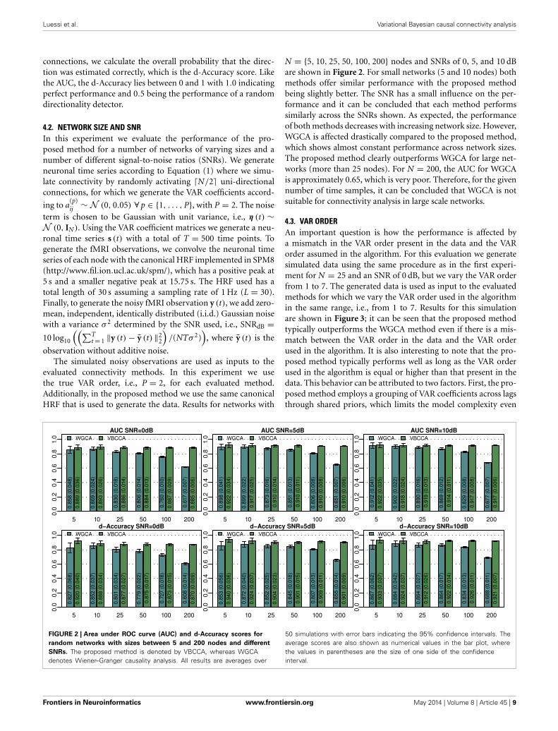
N = {5, 10, 25, 50, 100, 200} nodes and SNRs of 0, 5, and 10 dBare shown in Figure 2. For small networks (5 and 10 nodes) bothmethods offer similar performance with the proposed methodbeing slightly better. The SNR has a small influence on the per-formance and it can be concluded that each method performssimilarly across the SNRs shown. As expected, the performanceof both methods decreases with increasing network size. However,WGCA is affected drastically compared to the proposed method,which shows almost constant performance across network sizes.The proposed method clearly outperforms WGCA for large net-works (more than 25 nodes). For N = 200, the AUC for WGCAis approximately 0.65, which is very poor. Therefore, for the givennumber of time samples, it can be concluded that WGCA is notsuitable for connectivity analysis in large scale networks.

4.3. VAR ORDERAn important question is how the performance is affected bya mismatch in the VAR order present in the data and the VARorder assumed in the algorithm. For this evaluation we generatesimulated data using the same procedure as in the first experi-ment for N = 25 and an SNR of 0 dB, but we vary the VAR orderfrom 1 to 7. The generated data is used as input to the evaluatedmethods for which we vary the VAR order used in the algorithmin the same range, i.e., from 1 to 7. Results for this simulationare shown in Figure 3; it can be seen that the proposed methodtypically outperforms the WGCA method even if there is a mis-match between the VAR order in the data and the VAR orderused in the algorithm. It is also interesting to note that the pro-posed method typically performs well as long as the VAR orderused in the algorithm is equal or higher than that present in thedata. This behavior can be attributed to two factors. First, the pro-posed method employs a grouping of VAR coefficients across lagsthrough shared priors, which limits the model complexity even

FIGURE 2 | Area under ROC curve (AUC) and d-Accuracy scores for

random networks with sizes between 5 and 200 nodes and different

SNRs. The proposed method is denoted by VBCCA, whereas WGCAdenotes Wiener–Granger causality analysis. All results are averages over

50 simulations with error bars indicating the 95% confidence intervals. Theaverage scores are also shown as numerical values in the bar plot, wherethe values in parentheses are the size of one side of the confidenceinterval.


http://www.fil.ion.ucl.ac.uk/spm/





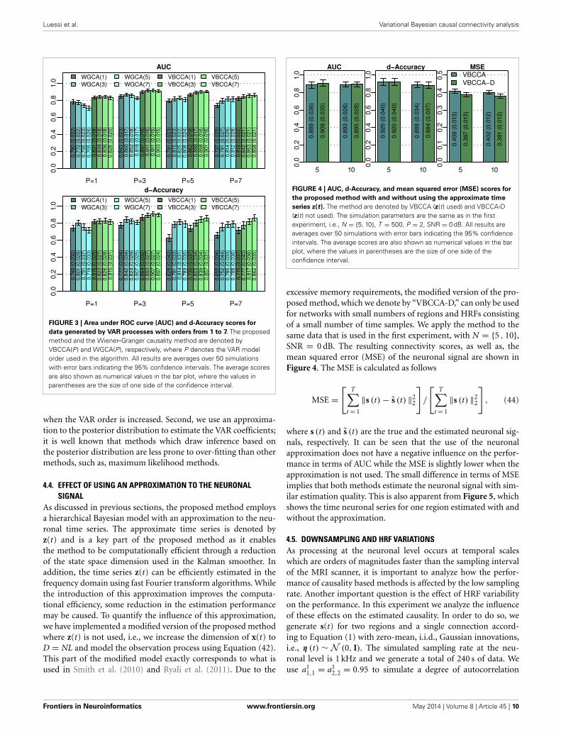
FIGURE 3 | Area under ROC curve (AUC) and d-Accuracy scores for

data generated by VAR processes with orders from 1 to 7. The proposedmethod and the Wiener–Granger causality method are denoted byVBCCA(P) and WGCA(P), respectively, where P denotes the VAR modelorder used in the algorithm. All results are averages over 50 simulationswith error bars indicating the 95% confidence intervals. The average scoresare also shown as numerical values in the bar plot, where the values inparentheses are the size of one side of the confidence interval.

when the VAR order is increased. Second, we use an approxima-tion to the posterior distribution to estimate the VAR coefficients;it is well known that methods which draw inference based onthe posterior distribution are less prone to over-fitting than othermethods, such as, maximum likelihood methods.

4.4. EFFECT OF USING AN APPROXIMATION TO THE NEURONALSIGNAL

As discussed in previous sections, the proposed method employsa hierarchical Bayesian model with an approximation to the neu-ronal time series. The approximate time series is denoted byz(t) and is a key part of the proposed method as it enablesthe method to be computationally efficient through a reductionof the state space dimension used in the Kalman smoother. Inaddition, the time series z(t) can be efficiently estimated in thefrequency domain using fast Fourier transform algorithms. Whilethe introduction of this approximation improves the computa-tional efficiency, some reduction in the estimation performancemay be caused. To quantify the influence of this approximation,we have implemented a modified version of the proposed methodwhere z(t) is not used, i.e., we increase the dimension of x(t) toD = NL and model the observation process using Equation (42).This part of the modified model exactly corresponds to what isused in Smith et al. (2010) and Ryali et al. (2011). Due to the

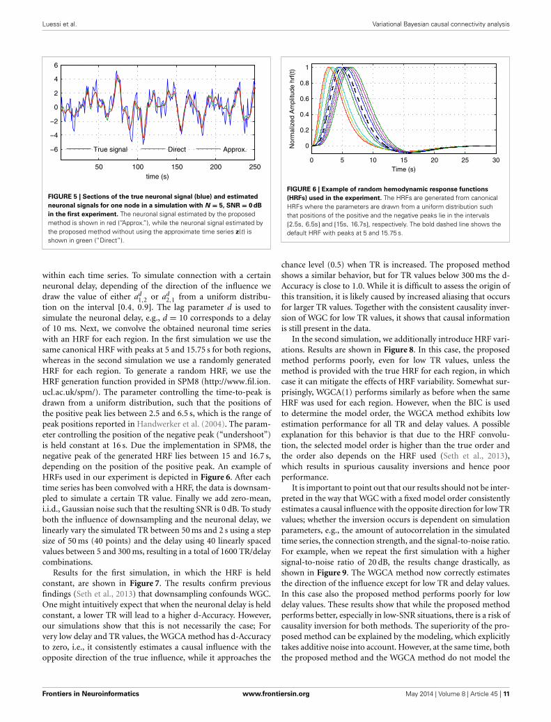
FIGURE 4 | AUC, d-Accuracy, and mean squared error (MSE) scores for

the proposed method with and without using the approximate time

series z(t). The method are denoted by VBCCA (z(t) used) and VBCCA-D(z(t) not used). The simulation parameters are the same as in the firstexperiment, i.e., N = {5, 10}, T = 500, P = 2, SNR = 0 dB. All results areaverages over 50 simulations with error bars indicating the 95% confidenceintervals. The average scores are also shown as numerical values in the barplot, where the values in parentheses are the size of one side of theconfidence interval.

excessive memory requirements, the modified version of the pro-posed method, which we denote by “VBCCA-D,” can only be usedfor networks with small numbers of regions and HRFs consistingof a small number of time samples. We apply the method to thesame data that is used in the first experiment, with N = {5 , 10},SNR = 0 dB. The resulting connectivity scores, as well as, themean squared error (MSE) of the neuronal signal are shown inFigure 4. The MSE is calculated as follows

MSE =[

T∑t = 1

‖s (t) − s (t) ‖22

]/

[T∑

t = 1

‖s (t) ‖22

], (44)

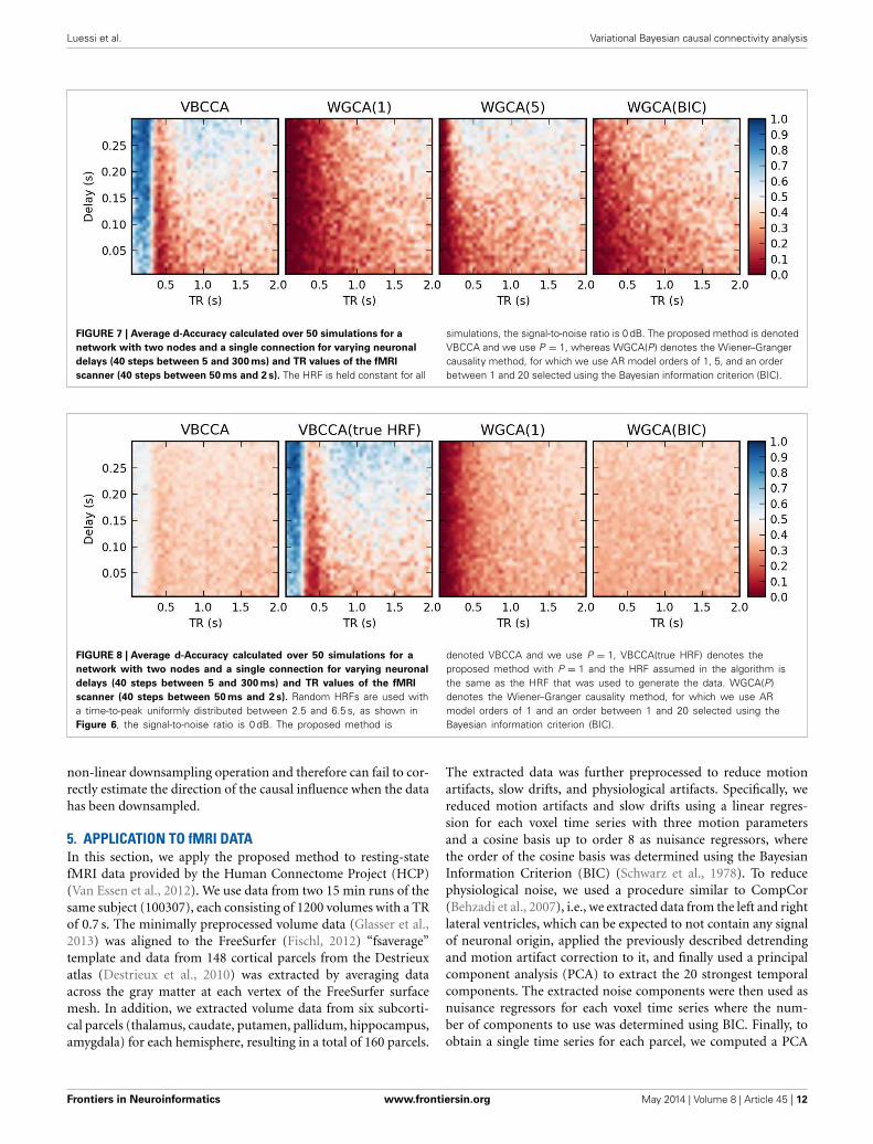
where s (t) and s (t) are the true and the estimated neuronal sig-nals, respectively. It can be seen that the use of the neuronalapproximation does not have a negative influence on the perfor-mance in terms of AUC while the MSE is slightly lower when theapproximation is not used. The small difference in terms of MSEimplies that both methods estimate the neuronal signal with sim-ilar estimation quality. This is also apparent from Figure 5, whichshows the time neuronal series for one region estimated with andwithout the approximation.

4.5. DOWNSAMPLING AND HRF VARIATIONSAs processing at the neuronal level occurs at temporal scaleswhich are orders of magnitudes faster than the sampling intervalof the MRI scanner, it is important to analyze how the perfor-mance of causality based methods is affected by the low samplingrate. Another important question is the effect of HRF variabilityon the performance. In this experiment we analyze the influenceof these effects on the estimated causality. In order to do so, wegenerate s(t) for two regions and a single connection accord-ing to Equation (1) with zero-mean, i.i.d., Gaussian innovations,i.e., η (t) ∼ N (0, I). The simulated sampling rate at the neu-ronal level is 1 kHz and we generate a total of 240 s of data. Weuse a1

1,1 = a12,2 = 0.95 to simulate a degree of autocorrelation






FIGURE 5 | Sections of the true neuronal signal (blue) and estimated

neuronal signals for one node in a simulation with N = 5, SNR = 0 dB

in the first experiment. The neuronal signal estimated by the proposedmethod is shown in red (“Approx.”), while the neuronal signal estimated bythe proposed method without using the approximate time series z(t) isshown in green (“Direct”).

within each time series. To simulate connection with a certainneuronal delay, depending of the direction of the influence wedraw the value of either ad

1,2 or ad2,1 from a uniform distribu-

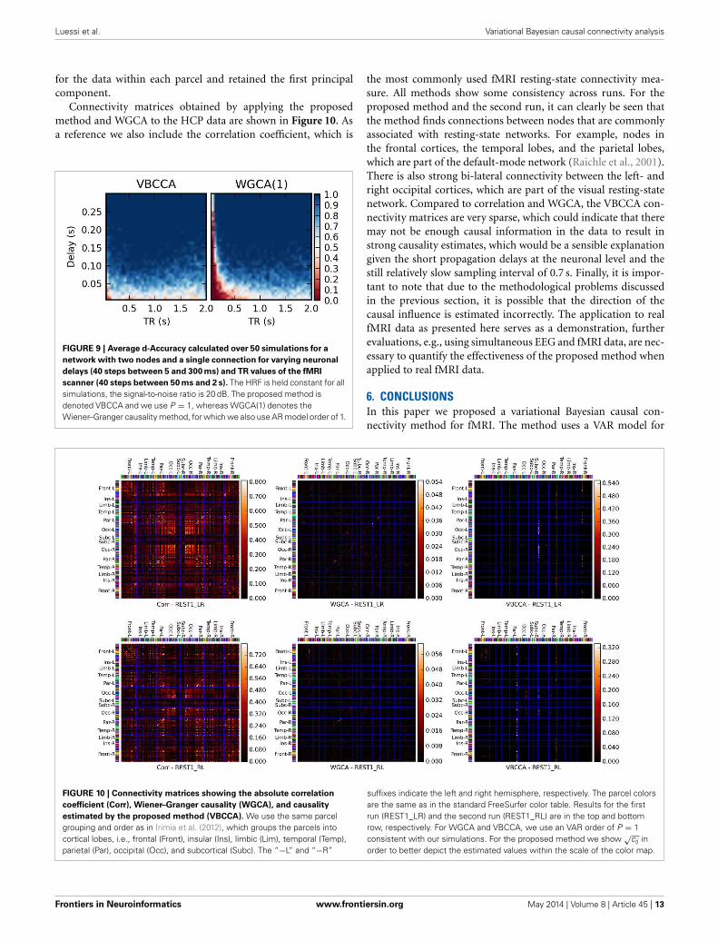
tion on the interval [0.4, 0.9]. The lag parameter d is used tosimulate the neuronal delay, e.g., d = 10 corresponds to a delayof 10 ms. Next, we convolve the obtained neuronal time serieswith an HRF for each region. In the first simulation we use thesame canonical HRF with peaks at 5 and 15.75 s for both regions,whereas in the second simulation we use a randomly generatedHRF for each region. To generate a random HRF, we use theHRF generation function provided in SPM8 (http://www.fil.ion.

ucl.ac.uk/spm/). The parameter controlling the time-to-peak isdrawn from a uniform distribution, such that the positions ofthe positive peak lies between 2.5 and 6.5 s, which is the range ofpeak positions reported in Handwerker et al. (2004). The param-eter controlling the position of the negative peak (“undershoot”)is held constant at 16 s. Due the implementation in SPM8, thenegative peak of the generated HRF lies between 15 and 16.7 s,depending on the position of the positive peak. An example ofHRFs used in our experiment is depicted in Figure 6. After eachtime series has been convolved with a HRF, the data is downsam-pled to simulate a certain TR value. Finally we add zero-mean,i.i.d., Gaussian noise such that the resulting SNR is 0 dB. To studyboth the influence of downsampling and the neuronal delay, welinearly vary the simulated TR between 50 ms and 2 s using a stepsize of 50 ms (40 points) and the delay using 40 linearly spacedvalues between 5 and 300 ms, resulting in a total of 1600 TR/delaycombinations.

Results for the first simulation, in which the HRF is heldconstant, are shown in Figure 7. The results confirm previousfindings (Seth et al., 2013) that downsampling confounds WGC.One might intuitively expect that when the neuronal delay is heldconstant, a lower TR will lead to a higher d-Accuracy. However,our simulations show that this is not necessarily the case; Forvery low delay and TR values, the WGCA method has d-Accuracyto zero, i.e., it consistently estimates a causal influence with theopposite direction of the true influence, while it approaches the

FIGURE 6 | Example of random hemodynamic response functions

(HRFs) used in the experiment. The HRFs are generated from canonicalHRFs where the parameters are drawn from a uniform distribution suchthat positions of the positive and the negative peaks lie in the intervals[2.5s, 6.5s] and [15s, 16.7s], respectively. The bold dashed line shows thedefault HRF with peaks at 5 and 15.75 s.

chance level (0.5) when TR is increased. The proposed methodshows a similar behavior, but for TR values below 300 ms the d-Accuracy is close to 1.0. While it is difficult to assess the origin ofthis transition, it is likely caused by increased aliasing that occursfor larger TR values. Together with the consistent causality inver-sion of WGC for low TR values, it shows that causal informationis still present in the data.

In the second simulation, we additionally introduce HRF vari-ations. Results are shown in Figure 8. In this case, the proposedmethod performs poorly, even for low TR values, unless themethod is provided with the true HRF for each region, in whichcase it can mitigate the effects of HRF variability. Somewhat sur-prisingly, WGCA(1) performs similarly as before when the sameHRF was used for each region. However, when the BIC is usedto determine the model order, the WGCA method exhibits lowestimation performance for all TR and delay values. A possibleexplanation for this behavior is that due to the HRF convolu-tion, the selected model order is higher than the true order andthe order also depends on the HRF used (Seth et al., 2013),which results in spurious causality inversions and hence poorperformance.

It is important to point out that our results should not be inter-preted in the way that WGC with a fixed model order consistentlyestimates a causal influence with the opposite direction for low TRvalues; whether the inversion occurs is dependent on simulationparameters, e.g., the amount of autocorrelation in the simulatedtime series, the connection strength, and the signal-to-noise ratio.For example, when we repeat the first simulation with a highersignal-to-noise ratio of 20 dB, the results change drastically, asshown in Figure 9. The WGCA method now correctly estimatesthe direction of the influence except for low TR and delay values.In this case also the proposed method performs poorly for lowdelay values. These results show that while the proposed methodperforms better, especially in low-SNR situations, there is a risk ofcausality inversion for both methods. The superiority of the pro-posed method can be explained by the modeling, which explicitlytakes additive noise into account. However, at the same time, boththe proposed method and the WGCA method do not model the








FIGURE 7 | Average d-Accuracy calculated over 50 simulations for a

network with two nodes and a single connection for varying neuronal

delays (40 steps between 5 and 300 ms) and TR values of the fMRI

scanner (40 steps between 50 ms and 2 s). The HRF is held constant for all

simulations, the signal-to-noise ratio is 0 dB. The proposed method is denotedVBCCA and we use P = 1, whereas WGCA(P) denotes the Wiener–Grangercausality method, for which we use AR model orders of 1, 5, and an orderbetween 1 and 20 selected using the Bayesian information criterion (BIC).




scanner (40 steps between 50 ms and 2 s). Random HRFs are used witha time-to-peak uniformly distributed between 2.5 and 6.5 s, as shown inFigure 6, the signal-to-noise ratio is 0 dB. The proposed method is

denoted VBCCA and we use P = 1, VBCCA(true HRF) denotes theproposed method with P = 1 and the HRF assumed in the algorithm isthe same as the HRF that was used to generate the data. WGCA(P)denotes the Wiener–Granger causality method, for which we use ARmodel orders of 1 and an order between 1 and 20 selected using theBayesian information criterion (BIC).

non-linear downsampling operation and therefore can fail to cor-rectly estimate the direction of the causal influence when the datahas been downsampled.

5. APPLICATION TO fMRI DATAIn this section, we apply the proposed method to resting-statefMRI data provided by the Human Connectome Project (HCP)(Van Essen et al., 2012). We use data from two 15 min runs of thesame subject (100307), each consisting of 1200 volumes with a TRof 0.7 s. The minimally preprocessed volume data (Glasser et al.,2013) was aligned to the FreeSurfer (Fischl, 2012) “fsaverage”template and data from 148 cortical parcels from the Destrieuxatlas (Destrieux et al., 2010) was extracted by averaging dataacross the gray matter at each vertex of the FreeSurfer surfacemesh. In addition, we extracted volume data from six subcorti-cal parcels (thalamus, caudate, putamen, pallidum, hippocampus,amygdala) for each hemisphere, resulting in a total of 160 parcels.

The extracted data was further preprocessed to reduce motionartifacts, slow drifts, and physiological artifacts. Specifically, wereduced motion artifacts and slow drifts using a linear regres-sion for each voxel time series with three motion parametersand a cosine basis up to order 8 as nuisance regressors, wherethe order of the cosine basis was determined using the BayesianInformation Criterion (BIC) (Schwarz et al., 1978). To reducephysiological noise, we used a procedure similar to CompCor(Behzadi et al., 2007), i.e., we extracted data from the left and rightlateral ventricles, which can be expected to not contain any signalof neuronal origin, applied the previously described detrendingand motion artifact correction to it, and finally used a principalcomponent analysis (PCA) to extract the 20 strongest temporalcomponents. The extracted noise components were then used asnuisance regressors for each voxel time series where the num-ber of components to use was determined using BIC. Finally, toobtain a single time series for each parcel, we computed a PCA






for the data within each parcel and retained the first principalcomponent.

Connectivity matrices obtained by applying the proposedmethod and WGCA to the HCP data are shown in Figure 10. Asa reference we also include the correlation coefficient, which is




scanner (40 steps between 50 ms and 2 s). The HRF is held constant for allsimulations, the signal-to-noise ratio is 20 dB. The proposed method isdenoted VBCCA and we use P = 1, whereas WGCA(1) denotes theWiener–Granger causality method, for which we also use AR model order of 1.

the most commonly used fMRI resting-state connectivity mea-sure. All methods show some consistency across runs. For theproposed method and the second run, it can clearly be seen thatthe method finds connections between nodes that are commonlyassociated with resting-state networks. For example, nodes inthe frontal cortices, the temporal lobes, and the parietal lobes,which are part of the default-mode network (Raichle et al., 2001).There is also strong bi-lateral connectivity between the left- andright occipital cortices, which are part of the visual resting-statenetwork. Compared to correlation and WGCA, the VBCCA con-nectivity matrices are very sparse, which could indicate that theremay not be enough causal information in the data to result instrong causality estimates, which would be a sensible explanationgiven the short propagation delays at the neuronal level and thestill relatively slow sampling interval of 0.7 s. Finally, it is impor-tant to note that due to the methodological problems discussedin the previous section, it is possible that the direction of thecausal influence is estimated incorrectly. The application to realfMRI data as presented here serves as a demonstration, furtherevaluations, e.g., using simultaneous EEG and fMRI data, are nec-essary to quantify the effectiveness of the proposed method whenapplied to real fMRI data.

6. CONCLUSIONSIn this paper we proposed a variational Bayesian causal con-nectivity method for fMRI. The method uses a VAR model for

FIGURE 10 | Connectivity matrices showing the absolute correlation

coefficient (Corr), Wiener–Granger causality (WGCA), and causality

estimated by the proposed method (VBCCA). We use the same parcelgrouping and order as in Irimia et al. (2012), which groups the parcels intocortical lobes, i.e., frontal (Front), insular (Ins), limbic (Lim), temporal (Temp),parietal (Par), occipital (Occ), and subcortical (Subc). The “−L” and “−R”

suffixes indicate the left and right hemisphere, respectively. The parcel colorsare the same as in the standard FreeSurfer color table. Results for the firstrun (REST1_LR) and the second run (REST1_RL) are in the top and bottomrow, respectively. For WGCA and VBCCA, we use an VAR order of P = 1consistent with our simulations. For the proposed method we show √cij inorder to better depict the estimated values within the scale of the color map.






the neuronal time series and the connectivity between regionsin combination with a hemodynamic convolution model. Byintroducing an approximation to the neuronal time series andperforming parts of the estimation in the frequency domain, ourmethod is computationally efficient and can be applied to largescale problems with several hundred ROIs and high samplingrates.

We performed simulations with synthetic data to evaluate theperformance of our method and to compare it with classicalWiener–Granger causality analysis (WGCA). There are severalimportant findings from these simulations that need further dis-cussion. In the first simulation, we demonstrated an importantstrength of our method, that is, it performs significantly bet-ter than WGCA when applied to problems with large numbersof regions. This effect is due to the use Gaussian priors for theVAR coefficients in combination with gamma priors for the pre-cision hyperparameters. This prior has a regularizing effect bypromoting sparsity for the VAR coefficients and can be seen asan adaptation of sparse Bayesian learning (Tipping, 2001) tothe problem of VAR coefficient estimation. In contrast, WGCAdoes not use regularization for the VAR coefficients resultingin a performance degradation when the number of regions isincreased. It is important to note that also the method in Ryaliet al. (2011) employs Gaussian-gamma priors for the VAR coef-ficients. However, due to the computational complexity of themethod it can only be applied to problems with small numbersof regions, where the prior is overwhelmed by the data and thesparsity promoting effect is of little benefit.

In the second set of simulations, we evaluated our methodusing simulated data generated by VAR processes of varyingorders. Again, due to the prior for the VAR coefficients, wherewe group coefficients across lags together using shared precisionhyperparameters, our method performed well as long as the VARorder used in the method is equal or higher than the VAR orderof the data. A grouping of VAR coefficients using �1�2-norm reg-ularization was first proposed in Haufe et al. (2008), in our workwe propose a Bayesian formulation for this problem.

In the third simulation, we analyzed the effect of using anapproximation to the neuronal time series, which is employed inour method to improve the computational efficiency, by compar-ing our method with a modified version of our method where theconvolution with the HRF is included in the observation matrixof the linear dynamic system, as in previous methods (Smith et al.,2010; Ryali et al., 2011). The simulation results show that theapproximation leads to some reduction in the quality of the esti-mated neuronal signal in terms of mean-squared error (MSE) butdoes not have a significant influence on the connectivity estima-tion performance. Importantly, the reduction in computationalcomplexity resulting from the use of the approximation to theneuronal signal allows us to apply the method to large scale prob-lems. As discussed above, the sparsity promoting priors for theVAR coefficients are of crucial importance when the method isapplied to problems with large numbers of regions. The use ofthe approximation to the neuronal time series is therefore animportant contribution of this work, as it allows us to apply themethod to problem sizes where the method can benefit from theregularizing effect of the priors.

In a last set of simulations, we analyzed the effect of differ-ent downsampling ratios, simulating different TR values of theMRI scanner, the neuronal delay, and HRF variability. Perhapsnot surprisingly, the proposed method is immune to HRF vari-ability if it has access to the true HRF of each region. Clearly,in practice HRFs are subject and region dependent. However, ithas been shown that HRFs are strongly correlated across sub-jects and regions (Handwerker et al., 2004). Hence, using datafrom a large number of subjects, it may be possible to con-struct a model describing the relationship between the HRFsin various brain regions. This “hemodynamic atlas” could thenbe used to approximate the HRFs in a large number of regionsfrom a small number of estimated HRFs for each subject. Wealso found that the proposed method generally performs bet-ter than WGC when a significant amount of additive noise ispresent in the data. This finding is consistent with previousresults (Seth et al., 2013) and can be explained by the modelused in the proposed method which can account for additivenoise. However, while the proposed method offers some benefitsover WGC, we find that also the proposed method can estimatea causal influence with the opposite direction when the datahas been downsampled, which is a known problem with WGCmethods (David et al., 2008; Deshpande et al., 2010; Seth et al.,2013). The problem that causality estimated using a discrete-time VAR model from a sampled continuous-time VAR processcan lead to opposite conclusions has been show before (Cox,1992). Unfortunately, this problem has received little attentionin recent work on causality estimation from fMRI data, wheresevere downsampling is common. In Solo (2007), it is shownthat while causality can be preserved under downsampling, VARmodels, as used in traditional WGC analysis and the proposedmethod, are inadequate for estimating causality from the sub-sampled time series and either VAR moving average (VARMA)models or state-space (SS) models are required to correctly esti-mate the direction of the causal influence. This raises hopesthat causality estimation from fMRI may be feasible by applyingmore sophisticated models to data acquired with low TR values,which may be achieved using a combination of novel acquisitionsequences and MRI scanners with higher field strengths. Clearly,HRF variability will still be a problem but under certain con-ditions it may be possible to use a model similar to the oneproposed in this work which can take into account the HRF ofeach region.

Finally, we applied the proposed method to real resting-statefMRI data provided by the Human Connectome Project (VanEssen et al., 2012). For this data, the proposed method findsconnections between regions that are associated with knownresting-state networks. However, it is important to emphasize thatapplication to real fMRI data as presented here serves as a demon-stration to show that the proposed method can be applied toreal fMRI data. As the true causal relationships in real data arenot known, it not possible to determine whether the direction ofcausal influence is correctly estimated. As shown in our simula-tions, there are methodological problems which, depending onthe noise level, the HRF, the TR, and the neuronal delay, can leadto causality inversions. Further experiments, e.g., using simulta-neous EEG and fMRI, are necessary to quantify the effectiveness






of the proposed method to estimate the direction of the causalinfluence from real fMRI data.

FUNDINGThis work was partially supported by the National Instituteof Child Health and Human Development (R01 HD042049).Martin Luessi was partially supported by the Swiss NationalScience Foundation Early Postdoc Mobility fellowship 148485.This work was supported in part by the Department of Energyunder Contract DE-NA0000457, the “Ministerio de Ciencia eInnovación” under Contract TIN2010-15137, and the CEI BioTicwith the Universidad de Granada Data were provided (in part)by the Human Connectome Project, WU-Minn Consortium(Principal Investigators: David Van Essen and Kamil Ugurbil;1U54MH091657) funded by the 16 NIH Institutes and Centersthat support the NIH Blueprint for Neuroscience Research;and by the McDonnell Center for Systems Neuroscience atWashington University.

REFERENCESAttias, H. (2000). A variational Bayesian framework for graphical models. Adv.

Neural Inform. Process. Syst. 12, 209–215.Babacan, S. D., Luessi, M., Molina, R., and Katsaggelos, A. K. (2012). Sparse

bayesian methods for low-rank matrix estimation. IEEE Trans. Signal Process.60, 3964–3977. doi: 10.1109/TSP.2012.2197748

Barnett, L., and Seth, A. K. (2011). Behaviour of Granger causality under filter-ing: theoretical invariance and practical application. J. Neurosci. Methods 201,404–419. doi: 10.1016/j.jneumeth.2011.08.010

Beal, M. J., and Ghahramani, Z. (2001). The Variational Kalman Smoother.Technical Report GCNU TR 2001-003, Gatsby Computational NeuroscienceUnit.

Behzadi, Y., Restom, K., Liau, J., and Liu, T. T. (2007). A component basednoise correction method (compcor) for {BOLD} and perfusion based fMRI.Neuroimage 37, 90–101. doi: 10.1016/j.neuroimage.2007.04.042

Bishop, C. M. (2006). Pattern Recognition and Machine Learning. New York, NY:Springer.

Bressler, S. L., and Seth, A. K. (2010). Wiener-Granger causality: a well establishedmethodology. Neuroimage 58, 323–329. doi: 10.1016/j.neuroimage.2010.02.059

Buxton, R. B., Uludag, K., Dubowitz, D. J., and Liu, T. T. (2004). Modeling thehemodynamic response to brain activation. Neuroimage 23, S220–S233. doi:10.1016/j.neuroimage.2004.07.013

Buxton, R. B., Wong, E. C., and Frank, L. R. (1998). Dynamics of blood flow andoxygenation changes during brain activation: the balloon model. Magn. Reson.Med. 39, 855–864. doi: 10.1002/mrm.1910390602

Cassidy, B., Long, C., Rae, C., and Solo, V. (2012). Identifying fMRI model viola-tions with lagrange multiplier tests. IEEE Trans. Med. Imaging 31, 1481–1492.doi: 10.1109/TMI.2012.2195327

Chaari, L., Vincent, T., Forbes, F., Dojat, M., and Ciuciu, P. (2013). Fastjoint detection-estimation of evoked brain activity in event-related fmriusing a variational approach. IEEE Trans. Med. Imaging 32, 821–837. doi:10.1109/TMI.2012.2225636

Cox, D. R. (1992). Causality: some statistical aspects. J. R. Stat. Soc. A, 291–301. doi:10.2307/2982962

David, O., Guillemain, I., and Saillet (2008). Identifying neural drivers withfunctional mri: an electrophysiological validation. PLoS Biol. 6:e315. doi:10.1371/journal.pbio.0060315

Deshpande, G., Sathian, K., and Hu, X. (2010). Effect of hemodynamic vari-ability on granger causality analysis of fMRI. Neuroimage 52, 884–896. doi:10.1016/j.neuroimage.2009.11.060

Destrieux, C., Fischl, B., Dale, A., and Halgren, E. (2010). Automatic parcella-tion of human cortical gyri and sulci using standard anatomical nomenclature.Neuroimage 53, 1–15. doi: 10.1016/j.neuroimage.2010.06.010

Fawcett, T. (2006). An introduction to roc analysis. Pattern Recogn. Lett. 27,861–874. doi: 10.1016/j.patrec.2005.10.010

Fernandes, P., Plateau, B., and Stewart, W. J. (1998). Efficient descriptor-vectormultiplications in stochastic automata networks. J. ACM (JACM) 45, 381–414.doi: 10.1145/278298.278303

Fischl, B. (2012). Freesurfer. Neuroimage 62, 774–781. doi:10.1016/j.neuroimage.2012.01.021

Frahm, J., Bruhn, H., Merboldt, K. D., and Math, D. (1992). Dynamic MR imagingof human brain oxygenation during rest and photic stimulation. J. Magn. Reson.Imaging 2, 501–505. doi: 10.1002/jmri.1880020505

Friston, K. J. (1994). Functional and effective connectivity in neuroimaging: asynthesis. Hum. Brain Mapping 2, 56–78. doi: 10.1002/hbm.460020107

Friston, K. J., Harrison, L., and Penny, W. (2003). Dynamic causal modelling.Neuroimage 19, 1273–1302. doi: 10.1016/S1053-8119(03)00202-7

Friston, K. J., Holmes, A. P., Poline, J. B., Grasby, P. J., Williams, S. C., Frackowiak,R. S., and Turner, R. (1995). Analysis of fMRI time-series revisited. Neuroimage2, 45–53. doi: 10.1006/nimg.1995.1007

Ghahramani, Z., and Beal, M. J. (2001). Propagation algorithms for variationalBayesian learning. Adv. Neural Inform. Process. Syst. 13, 507–513.

Ghahramani, Z., and Hinton, G. E. (1996). Parameter Estimation for LinearDynamical Systems. University of Toronto technical report CRG-TR-96-2, 6.

Glasser, M. F., Sotiropoulos, S. N., Wilson, J. A., Coalson, T. S., Fischl, B.,Andersson, J. L., et al. (2013). The minimal preprocessing pipelinesfor the human connectome project. Neuroimage 80, 105–124. doi:10.1016/j.neuroimage.2013.04.127

Granger, C. (1969). Investigating causal relations by econometric models and cross-spectral methods. Econ. J. Econ. Soc. 37, 424–438.

Handwerker, D. A., Ollinger, J. M., and D’Esposito, M. (2004). Variationof bold hemodynamic responses across subjects and brain regions andtheir effects on statistical analyses. Neuroimage 21, 1639–1651. doi:10.1016/j.neuroimage.2003.11.029

Haufe, S., Müller, K. R., Nolte, G., and Krämer, N. (2008). “Sparse causal discoveryin multivariate time series,” in NIPS Workshop on Causality, (Whistler).

Irimia, A., Chambers, M. C., Torgerson, C. M., Filippou, M., Hovda, D. A., Alger,J. R., et al. (2012). Patient-tailored connectomics visualization for the assess-ment of white matter atrophy in traumatic brain injury. Front. Neurol. 3:10. doi:10.3389/fneur.2012.00010

Jordan, M. I., Ghahramani, Z., Jaakkola, T. S., and Saul, L. K. (1999). An intro-duction to variational methods for graphical models. Mach. Learn. 37, 183–233.doi: 10.1023/A:1007665907178

Luessi, M. (2011). Bayesian Approaches to Inverse Problems in FunctionalNeuroimaging. Ph.D. thesis, Northwestern University.

Makni, S., Beckmann, C., Smith, S., and Woolrich, M. (2008). Bayesian deconvo-lution fMRI data using bilinear dynamical systems. Neuroimage 42, 1381–1396.doi: 10.1016/j.neuroimage.2008.05.052

Marinazzo, D., Liao, W., Chen, H., and Stramaglia, S. (2011). Nonlinearconnectivity by granger causality. Neuroimage 58, 330–338. doi:10.1016/j.neuroimage.2010.01.099

Meier, L., Geer, S., and Bühlmann, P. (2008). The group lasso for logistic regression.J. R. Stat. Soc. Ser. B 70, 53–71. doi: 10.1111/j.1467-9868.2007.00627.x

Moon, T. K., and Stirling, W. C. (2000). Mathematical Methods and Algorithms forSignal Processing, Vol. 204. New York, NY: Prentice Hall.

Ogawa, S., Lee, T., Kay, A., and Tank, D. (1990). Brain magnetic resonance imagingwith contrast dependent on blood oxygenation. Proc. Natl. Acad. Sci. U.S.A. 87,9868. doi: 10.1073/pnas.87.24.9868

Penny, W., Ghahramani, Z., and Friston, K. (2005). Bilinear dynamical systems.Philos. Trans. R. Soc. B Biol. Sci. 360, 983. doi: 10.1098/rstb.2005.1642

Raichle, M. E., MacLeod, A. M., Snyder, A. Z., Powers, W. J., Gusnard, D. A., andShulman, G. L. (2001). A default mode of brain function. Proc. Natl. Acad. Sci.U.S.A. 98, 676–682. doi: 10.1073/pnas.98.2.676

Rauch, H. E., Tung, F., and Striebel, C. (1965). Maximum likelihood estimates oflinear dynamic systems. AIAA J. 3, 1445–1450. doi: 10.2514/3.3166

Roebroeck, A., Seth, A. K., and Valdes-Sosa, P. (2011). Causal time seriesanalysis of functional magnetic resonance imaging data. J. Mach. Learn.Res. (Workshop and Conference Proceedings. Causality in Time Series) 12,65–94.

Ryali, S., Supekar, K., Chen, T., and Menon, V. (2011). Multivariate dynamicalsystems models for estimating causal interactions in fMRI. Neuroimage 54,807–823. doi: 10.1016/j.neuroimage.2010.09.052

Schwarz, G. et al. (1978). Estimating the dimension of a model. Annal. Stat. 6,461–464.






Seth, A. K. (2010). A matlab toolbox for granger causal connectivity analysis. J.Neurosci. Methods 186, 262–273. doi: 10.1214/aos/1176344136

Seth, A. K., Chorley, P., and Barnett, L. C. (2013). Granger causality analysis of fMRIBOLD signals is invariant to hemodynamic convolution but not downsampling.Neuroimage 65, 540–555. doi: 10.1016/j.neuroimage.2012.09.049

Smith, J. F., Pillai, A., Chen, K., and Horwitz, B. (2010). Identification and val-idation of effective connectivity networks in functional magnetic resonanceimaging using switching linear dynamic systems. Neuroimage 52, 1027–1040.doi: 10.1016/j.neuroimage.2009.11.081

Smith, S. M., Miller, K. L., Salimi-Khorshidi, G., Webster, M., Beckmann, C. F.,Nichols, T. E., et al. (2011). Network modelling methods for fMRI. Neuroimage54, 875–891. doi: 10.1016/j.neuroimage.2010.08.063

Solo, V. (2007). “On causality I: sampling and noise,” 2007 46th IEEEConference on Decision and Control (New Orleans, LA), 3634–3639. doi:10.1109/CDC.2007.4434049

Tipping, M. E. (2001). Sparse bayesian learning and the relevance vector machine.J. Mach. Learn. Res. 1, 211–244.

Valdés-Sosa, P. A., Sánchez-Bornot, J. M., Lage-Castellanos, A., Vega-Hernández,M., Bosch-Bayard, J., Melie-García, L., et al. (2005). Estimating brain func-tional connectivity with sparse multivariate autoregression. Philos. Trans. R. Soc.B Biol. Sci. 360, 969. doi: 10.1098/rstb.2005.1654

Van Essen, D. C., Ugurbil, K., Auerbach, E., Barch, D., Behrens, T. E. J., Bucholz, R.,et al. (2012). The human connectome project: a data acquisition perspective.Neuroimage 62, 2222–2231. doi: 10.1016/j.neuroimage.2012.02.018

Wang, B., and Titterington, D. (2004). Lack of consistency of mean field and vari-ational bayes approximations for state space models. Neural Process. Lett. 20,151–170. doi: 10.1007/s11063-004-2024-6

Weigend, A. S., and Gershenfeld, N. A. (1994). Time Series Prediction: Forecastingthe Future and Understanding the Past. Reading, MA: Addison-Wesley.

Wiener, N. (1956). The theory of prediction. Modern mathematics for engineers.New York, NY: McGraw-Hill.

Wipf, D. P., and Rao, B. D. (2007). An Empirical Bayesian Strategy for Solving theSimultaneous Sparse Approximation Problem. IEEE Trans. Signal Process. 55,3704–3716. doi: 10.1109/TSP.2007.894265

Yuan, M., and Lin, Y. (2006). Model selection and estimation in regression withgrouped variables. J. R. Stat. Soc. Ser. B (Statistical Methodology) 68, 49–67. doi:10.1111/j.1467-9868.2005.00532.x

Conflict of Interest Statement: The authors declare that the research was con-ducted in the absence of any commercial or financial relationships that could beconstrued as a potential conflict of interest.

Received: 05 January 2014; accepted: 01 April 2014; published online: 05 May 2014.Citation: Luessi M, Babacan SD, Molina R, Booth JR and Katsaggelos AK (2014)Variational Bayesian causal connectivity analysis for fMRI. Front. Neuroinform. 8:45.doi: 10.3389/fninf.2014.00045This article was submitted to the journal Frontiers in Neuroinformatics.Copyright © 2014 Luessi, Babacan, Molina, Booth and Katsaggelos. This is anopen-access article distributed under the terms of the Creative Commons AttributionLicense (CC BY). The use, distribution or reproduction in other forums is permit-ted, provided the original author(s) or licensor are credited and that the originalpublication in this journal is cited, in accordance with accepted academic practice.No use, distribution or reproduction is permitted which does not comply with theseterms.


http://dx.doi.org/10.3389/fninf.2014.00045



http://creativecommons.org/licenses/by/3.0/








Documents

Variational Bayesian causal connectivity analysis for fMRI · convolution with a hemodynamic response function. Due to the employed modeling, it is Due to the employed modeling, it