Various Model Types

Tony Hürlimann

tony.huerlimann@unifr.ch

Department of Informatics

University of Fribourg

February 1, 2021

Abstract

Several model types are formulated in mathematical notation and in the mod-elling system LPL (see [5]). They are compared with each other from various pointof views. Then we give a concrete model application example for each model type.

(This PDF-document (variants.pdf) was generated automatically from the Latex�le variants.tex and the LPL source �les using LPL's own automatic documentationtool.)

1

Contents

1 Introduction 3

2 A Linear Program (examp-lp) 6

3 A Integer Linear Program (examp-ip) 10

4 A 0-1 Integer Program (examp-ip01) 14

5 An LP-relaxation of the 0-1 program (examp-ip01r) 17

6 A Quadratic Convexe Program (examp-qp) 21

7 A 0-1-Quadratic Program (examp-qp01) 24

8 Conclusion 27

2

1 Introduction

In this paper, a general overview of various mathematical optimization model types is pre-sented. A general speci�cation and formulation is given �rst in a mathematical notationthen in the modelling language LPL (see [5]).

A mathematical model has the following general form:

min f(x)subject to gi(x) ≤ 0 forall i = 1, . . . ,m

x ∈ X

where f and gi are functions de�ned in Rn. X is a subset of Rn, and x is a vector of ncomponents x1, . . . , xn. The above problem has to be solved for the values of the variablesx1, . . . , xn that satisfy the restrictions gi while minimizing the function f . The functionf is called the objective function, gi are the constraints. A vector x ∈ X that satis�es allconstraints gi(x) ≤ 0 is called feasible solution. The collection of all such points is thefeasible region. The problem then of the mathematical model above is to �nd a xo suchthat f(x) ≥ f(xo) for each feasible point x. Such a point xo is called an optimal solution.

A small example is the following model (see [3], page 3):

min (x1 − 3)2 + (x2 − 2)2

subject to x21x2 − 3 ≤ 0x2 − 1 ≤ 0−x1 ≤ 0

The objective function and the constraints are:

f(x1, x2) = (x1 − 3)2 + (x2 − 2)2

g1(x1, x2) = x21x2 − 3 ≤ 0g2(x1, x2) = x2 − 1 ≤ 0g3(x1, x2) = −x1 ≤ 0

Figure 1 illustrates the model geometrically in the two-dimensional real Euclideanspace.

There are useful practical variations of the standard model:

1. The objective function can be a maximizing function:

max f(x)

To translate it into a standard form, one only needs to write it as :

min −f(x)

2. The variables x in a standard model are free. If they must be positive, then one caneasily add the constraints: (x ≥ 0).

3. If the constraints are gi(x) ≥ 0, they can be replaced by −gi(x) ≤ 0.

4. If the constraints are gi(x) = 0, they can be replaced by gi(x) ≥ 0 and gi(x) ≤ 0constraints.

3

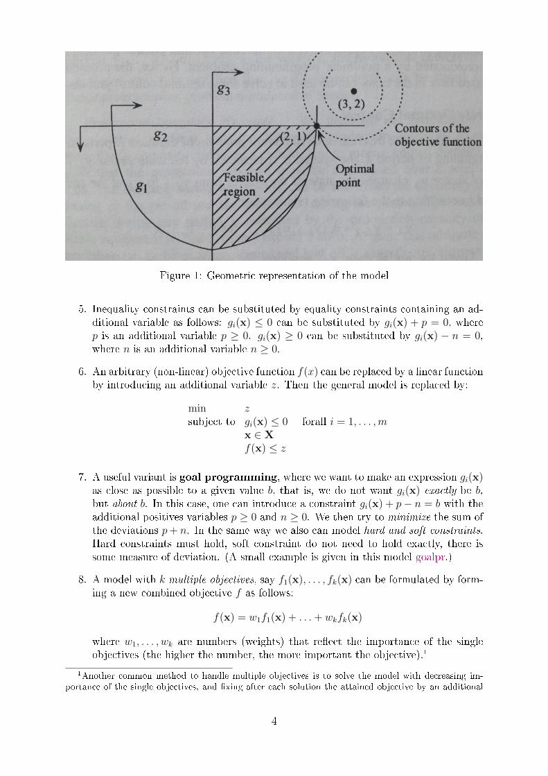
Figure 1: Geometric representation of the model

5. Inequality constraints can be substituted by equality constraints containing an ad-ditional variable as follows: gi(x) ≤ 0 can be substituted by gi(x) + p = 0, wherep is an additional variable p ≥ 0. gi(x) ≥ 0 can be substituted by gi(x) − n = 0,where n is an additional variable n ≥ 0.

6. An arbitrary (non-linear) objective function f(x) can be replaced by a linear functionby introducing an additional variable z. Then the general model is replaced by:

min zsubject to gi(x) ≤ 0 forall i = 1, . . . ,m

x ∈ Xf(x) ≤ z

7. A useful variant is goal programming, where we want to make an expression gi(x)as close as possible to a given value b, that is, we do not want gi(x) exactly be b,but about b. In this case, one can introduce a constraint gi(x) + p− n = b with theadditional positives variables p ≥ 0 and n ≥ 0. We then try to minimize the sum ofthe deviations p+ n. In the same way we also can model hard and soft constraints.Hard constraints must hold, soft constraint do not need to hold exactly, there issome measure of deviation. (A small example is given in this model goalpr.)

8. A model with k multiple objectives, say f1(x), . . . , fk(x) can be formulated by form-ing a new combined objective f as follows:

f(x) = w1f1(x) + . . .+ wkfk(x)

where w1, . . . , wk are numbers (weights) that re�ect the importance of the singleobjectives (the higher the number, the more important the objective).1

1Another common method to handle multiple objectives is to solve the model with decreasing im-portance of the single objectives, and �xing after each solution the attained objective by an additional

4

In an application, the objective function may have various meaning. We may max-imize pro�t, utility, turnover, return on investment, net present value, number of employ-ees, customer satisfaction, probability of survival, robustness; or we may minimize cost,number of employees, redundancy, deviations, use of resources, etc.

The constraints re�ect a large variation of requirements in a concrete application.In a production context there may be capacity, material availability marketing limita-tion, material balance constraints; in a resource scheduling we may have due date, jobsequencing, space limitation constraints; etc.

In the following sections various model types are presented: (1) Linear programs (LP)consist of linear constraints and a linear objective function and real variables. (2) Integer(linear) programs (IP) consist of linear constraints and a linear objective function andinteger variables. (3) 0 − 1 (linear) programs consist of linear constraints and a linearobjective function and binary variables. This type is a special case of (2), where variablesare integer but can only take the values 0 or 1. From the formulation point of view,the di�erence between the three types is very small. However � as we shall see � thedi�culty to solve integer problems is much higher. Linear programs (LP) can be solvedin polynomial time, while IP and 0 − 1 IP problems are NP-complete. The application�eld of these three model types is very large. We shall see examples.

In addition, there exist (4) quadratic problems (QP) which consist of linear constraintsand a quadratic convex objective function. (5) 0-1 quadratic problems (0− 1-QP) whichconsist of linear constraints and a quadratic convex objective function and contain 0− 1variables. Both types have interesting applications in portfolio theory. (6) Quadraticconstraint problems (QCP) which consist of linear and quadratic convex constraints anda quadratic convex objective function. Finally, we add (7) second order cone problems(SOCP), which have many applications in physics. Of course, there is the large part ofmodel types that are non-linear. We also shall see examples.

For each of the model types, a concrete application and an implementation in LPLis given. We shall show the gap in di�culty to solve integer problems compared to non-integer problems.

Of course, one can also build combined models: LP model part mixed with IP modelleads to mixed integer programs (MIP) containing real and integer variables.

constraint: Hence, solve the model �rst with fh(x) (supposing fh is the most important objective). Letthe optimal value be fo

h , then add the constraint gm+1(x) = fh(x)− foh = 0. Now continue in the same

way with the second most important objective, an so on until the least important objective (a modelwhere this technique is used can be found here: library).

5

2 A Linear Program (examp-lp)

Problem: The general linear programming model � called LP � consists of a linearobjective function f(x) andm linear constraints gi(x) and n variables. It can be compactlyformulated as follows (see [6]):

min∑j∈J

cjxj

subject to∑j∈J

ai,jxj ≥ bi forall i ∈ I

xj ≥ 0 forall j ∈ Jwith I = {1 . . .m}, J = {1 . . . n}, m, n ≥ 0

An more compact formulation using matrix notation for the model is as follows:

min c · xsubject to A · x ≥ b

x ≥ 0

The objective function f the constraints gi, and X (in the general format) are as follows:

f(x1, . . . , xn) = c1x1 + . . .+ cnxngi(x1, . . . , xn) = bi − (ai,1x1 + . . .+ ai,nxn) ≤ 0 for i = 1, . . . ,m

x ∈ Rn

Note that in addition to the gi constraints we also have the non-negativity conditionson the variables x in the standard formulation. If we need negative variables, we mustexplicitly replace x by x1 − x2, where x1,x2 ≥ 0 are two positive vectors ∈ Rn.

In the following, a concrete problem with random data for the matrix A, and the twovectors b and c is speci�ed (with n = 15 and m = 15):

c =(16 73 39 81 68 60 90 11 33 89 71 12 24 23 47

)

A =

87 34 0 0 43 0 52 85 36 0 0 0 0 0 00 0 39 0 84 0 0 88 0 0 0 0 0 0 2255 63 79 0 0 0 0 71 0 0 0 0 70 0 790 0 0 0 0 0 0 73 0 0 0 22 0 0 00 0 0 66 0 0 34 0 0 24 0 61 0 0 640 0 16 19 0 0 0 0 0 0 0 0 0 0 1815 70 61 0 0 0 0 0 0 0 0 0 0 0 00 0 0 0 0 0 0 0 52 0 14 0 0 92 00 0 0 0 0 0 0 30 0 0 98 0 19 0 00 70 37 0 0 0 0 0 0 0 0 86 0 93 090 0 82 0 66 0 0 0 0 26 0 0 0 0 077 30 0 0 0 0 13 10 0 0 0 50 0 0 00 0 0 0 0 0 0 0 0 0 0 0 0 0 00 72 0 0 0 79 0 0 0 0 0 11 90 0 00 0 0 0 0 32 55 0 23 0 0 0 0 0 36

b =

0000000584400000

119

6

With these data, the model is speci�ed by the following explicit linear program:

min 16x1 + 73x2 + 39x3 + 81x4 + 68x5 + 60x6 + 90x7 + 11x8 + 33x9+89x10 + 71x11 + 12x12 + 24x13 + 23x14 + 47x15

subject to 87x1 + 34x2 + 43x5 + 52x7 + 85x8 + 36x9 ≥ 039x3 + 84x5 + 88x8 + 22x15 ≥ 055x1 + 63x2 + 79x3 + 71x8 + 70x13 + 79x15 ≥ 073x8 + 22x12 ≥ 066x4 + 34x7 + 24x10 + 61x12 + 64x15 ≥ 016x3 + 19x4 + 18x15 ≥ 015x1 + 70x2 + 61x3 ≥ 052x9 + 14x11 + 92x14 ≥ 5830x8 + 98x11 + 19x13 ≥ 4470x2 + 37x3 + 86x12 + 93x14 ≥ 090x1 + 82x3 + 66x5 + 26x10 ≥ 077x1 + 30x2 + 13x7 + 10x8 + 50x12 ≥ 072x2 + 79x6 + 11x12 + 90x13 ≥ 032x6 + 55x7 + 23x9 + 36x15 ≥ 119xj ≥ 0 forall j ∈ {1 . . . 15}

Modeling Steps

The formulation of the model in the LPL modeling language is straightforward and thenotation is close to the mathematical notation using indices: First we de�ne the two setsi and j. Then we declare and assign the data as parameters A, c, and b. The variablevector x is declared, and �nally the constraints R and the minimizing objective functionobj are written.

Note that the data matrices A, b, and c are generated using LPL's own randomgenerator. (To generate each time the same data, the code can also use the functionSetRandomSeed(a) where a is an integer.)

Listing 1: The Complete Model in LPL [5]� �model Lp15 "A Linear Program";

set i := [1..15]; j := [1..15];parameter A{i,j}:= Trunc(if(Rnd(0,1)<.25,Rnd(10,100)));

c{j} := Trunc(Rnd(10,100));b{i} := Trunc(if(Rnd(0,1)<.15,Rnd(0,120)));

variable x{j};constraint R{i} : sum{j} A*x >= b;minimize obj : sum{j} c*x;Writep(obj,x);

end� �Today, models with n,m > 10000 and much larger are solved on a regular base. LP

models with millions of variables can be solved today. A linear programming model with2000 variables and 1000 linear constraints can be downloaded and solved at: lp20002.

Solution: The small model de�ned above has the following solution:

x =(0 0 0 0 0 0 0 1.4667 1.1154 0 0 0 0 0 2.5929

)2 http://lpl.virtual-optima.com/lpl/Solver.jsp?name=/lp2000

7

The optimal value of the objective function is:

obj = 174.8096

Further Comments: The linear programming (LP) model has many applications inquantitative decision making. LP is used for capacity planning, resource (raw material)allocation, manpower planning, blending, transportation, network �ow, network design,portfolio selection, optimal marketing mix, multiperiod product mix, and many others.

A small example in multi period production planning is given in the model: product3.A historical example of a the so-called diet problem is modeled by diet4. An applicationof sca�olding � arrangement of beams and ropes � can be found here: sca�olding5. Afurther problem from game theory to �nd the optimal strategy of a 2-person game is givenin the problem: gameh6. A linear model implementing three common regression methodsis given in regression7.

Further Notes: As already seen in the two models gameh and regression certain non-linear functions can be transformed in a way that the model becomes an linear one. Wemention three of them (see [1], Chap. 13):

1. The absolute value. Suppose the objective function has the form:

f(x) = |c · x|

One can add a single variable y and modify the LP as follows:

min ysubject to A · x ≥ b

c · x ≤ y−c · x ≤ yx ≥ 0y ≥ 0

This can be generatized. If the objective function is:

f(x) =∑i∈I

|ci · x|

One can add a vector of variables yi (with i ∈ I) and modify the LP as follows:

min∑

i∈I yisubject to A · x ≥ b

ci · x ≤ yi , forall i ∈ I−ci · x ≤ yi , forall i ∈ Ix ≥ 0yi ≥ 0 , forall i ∈ I

3 http://lpl.virtual-optima.com/lpl/Solver.jsp?name=/product4 http://lpl.virtual-optima.com/lpl/Solver.jsp?name=/diet5 http://lpl.virtual-optima.com/lpl/Solver.jsp?name=/sca�olding6 http://lpl.virtual-optima.com/lpl/Solver.jsp?name=/gameh7 http://lpl.virtual-optima.com/lpl/Solver.jsp?name=/regression

8

2. The maximal value. Suppose the objective function has the form:

f(x) = max c · x

One can add a single variable y and modify the LP as follows:

min ysubject to A · x ≥ b

c · x ≤ yx ≥ 0y ≥ 0

In a similar way, if the objective function is:

f(x) = maxi∈I|ci · x|

One can add a single variable y and modify the LP as follows:

min∑

i∈I yisubject to A · x ≥ b

ci · x ≤ y , forall i ∈ I−ci · x ≤ y , forall i ∈ Ix ≥ 0yi ≥ 0 , forall i ∈ I

3. The fractional LP. Suppose the objective function consists of maximizing the ratioof two linear functions (where p and q are two data vectors and α and β are twoscalars):

f(x) =p · x+ α

q · x+ β

One can convert this into a LP model. If the feasible set {x|A · x ≤ b,x ≤ 0} isnonempty and bounded and if q · x+ β > 0, using the following transformations:

z =1

q · x+ β, y = zx

we obtain the following LP:

min p · x+ αsubject to A · y − bz ≤ 0

q · y + βz = 1y ≥ 0z ≥ 0

A small example is given in Bill0468.

8 http://lpl.virtual-optima.com/lpl/Solver.jsp?name=/Bill046

9

3 A Integer Linear Program (examp-ip)

Problem: The general linear integer programming model � called IP � contains alinear objective function f(x), m linear constraints gi(x), and n integer variables. It canbe compactly formulated as follows (see [6]):

min∑j∈J

cjxj

subject to∑j∈J

ai,jxj ≥ bi forall i ∈ I

xj ∈ N+ forall j ∈ Jwith I = {1 . . .m}, J = {1 . . . n}, m, n ≥ 0

A more compact formulation using matrix notation for the model is :

min c · xsubject to A · x ≥ b

x ∈ N+

The objective function f , the constraints gi, and x (in the general model format) are asfollows:

f(x1, . . . , xn) = c1x1 + . . .+ cnxngi(x1, . . . , xn) = bi − (ai,1x1 + . . .+ ai,nxn) ≤ 0 for i = 1, . . . ,m

x ∈ Nn

The IP model has the same notation as the LP model, the only di�erence is that thevariables are integer values. However, IP model are much more di�cult to solve in general.(To get an idea solve the following model: lp20009. Then try to solve ip200010.)

In the following a problem with random data is speci�ed (with n = 15 and m = 15):

c =(16 73 39 81 68 60 90 11 33 89 71 12 24 23 47

)

A =

87 34 0 0 43 0 52 85 36 0 0 0 0 0 00 0 39 0 84 0 0 88 0 0 0 0 0 0 2255 63 79 0 0 0 0 71 0 0 0 0 70 0 790 0 0 0 0 0 0 73 0 0 0 22 0 0 00 0 0 66 0 0 34 0 0 24 0 61 0 0 640 0 16 19 0 0 0 0 0 0 0 0 0 0 1815 70 61 0 0 0 0 0 0 0 0 0 0 0 00 0 0 0 0 0 0 0 52 0 14 0 0 92 00 0 0 0 0 0 0 30 0 0 98 0 19 0 00 70 37 0 0 0 0 0 0 0 0 86 0 93 090 0 82 0 66 0 0 0 0 26 0 0 0 0 077 30 0 0 0 0 13 10 0 0 0 50 0 0 00 0 0 0 0 0 0 0 0 0 0 0 0 0 00 72 0 0 0 79 0 0 0 0 0 11 90 0 00 0 0 0 0 32 55 0 23 0 0 0 0 0 36

b =

0000000584400000119

9 http://lpl.virtual-optima.com/lpl/Solver.jsp?name=/lp200010 http://lpl.virtual-optima.com/lpl/Solver.jsp?name=/ip2000

10

The data given above specify the following explicit linear program:

min 16x1 + 73x2 + 39x3 + 81x4 + 68x5 + 60x6 + 90x7 + 11x8 + 33x9+89x10 + 71x11 + 12x12 + 24x13 + 23x14 + 47x15

subject to 87x1 + 34x2 + 43x5 + 52x7 + 85x8 + 36x9 ≥ 039x3 + 84x5 + 88x8 + 22x15 ≥ 055x1 + 63x2 + 79x3 + 71x8 + 70x13 + 79x15 ≥ 073x8 + 22x12 ≥ 066x4 + 34x7 + 24x10 + 61x12 + 64x15 ≥ 016x3 + 19x4 + 18x15 ≥ 015x1 + 70x2 + 61x3 ≥ 052x9 + 14x11 + 92x14 ≥ 5830x8 + 98x11 + 19x13 ≥ 4470x2 + 37x3 + 86x12 + 93x14 ≥ 090x1 + 82x3 + 66x5 + 26x10 ≥ 077x1 + 30x2 + 13x7 + 10x8 + 50x12 ≥ 072x2 + 79x6 + 11x12 + 90x13 ≥ 032x6 + 55x7 + 23x9 + 36x15 ≥ 119xj ∈ N+ forall j ∈ {1 . . . 15}

Modeling Steps

The formulation of the model in LPL modeling language is straightforward and the no-tation is close to the mathematical notation using indices: First we de�ne the two setsi and j. Then we declare and assign the data as parameters A, c, and b. The variablevector x is declared with the keyword integer (the only di�erence to the LP model),and �nally the constraints R and the minimizing objective function obj are written.

Note that the data matrices A, b, and c are generated using LPL's own randomgenerator. (To generate the same data each time, the code can also use the functionSetRandomSeed(a) where a is an integer.)

Listing 2: The Complete Model in LPL [5]� �model Ip15 "A In t eg e r Linear Program";

set i := [1..15]; j := [1..15];parameter A{i,j} := Trunc(if(Rnd(0,1)<0.25, Rnd(10,100)));

c{j} := Trunc(Rnd(10,100));b{i} := Trunc(if(Rnd(0,1)<0.15, Rnd(0,120)));

integer variable x{j};constraint R{i} : sum{j} A*x >= b;minimize obj : sum{j} c*x;Writep(obj,x);

end� �Solution: The small model de�ned above has the following solution :

x =(0 0 0 0 0 0 0 2 4 0 0 0 0 0 1

)

11

The optimal value of the objective function is:

obj = 201

If we compare this solution with the corresponding LP model in examp-lp11, we noticethat the objective value is much larger (201 compared to 174.8096). Furthermore, thevector x is not simply the �round-down� of the LP solution, as one may expect. Tounderstand why we cannot simply round up or down to get an integer solution froma corresponding LP model, open the model willi15512 and read the modeling text tounderstand why.

Further Comments: IP problems are much more di�cult to solve than LP problemsin general. However, there is a surprisingly rich application �eld for integer programs.Obvious applications are problems where we have indivisible objects, such as number ofpersons, machines, etc. However, these are not typical applications. If we have the numberof drivers in a small company then we may model this as an integer quantity, however ifwe have the population in a country then we may approximate it as a continuous variable.This obvious aspect, however, does not reveal the real power of integer programming. Wereally need integer programming in the four following contexts in this order of importancefrom a practical point of view:

1. To model problems with logical conditions. In this case, the integrality is evenreduced to variables that only take the value 0 or 1 (see the next model examp-ip0113) for more information about them and how to specify logical constraints).

2. To model combinatorial problems, such as sequencing problems, (job-shop) schedul-ing, and many others. Many of them are again transformed to integer problemswith 0− 1 variables. A small example can be found here: words14.

3. To model non-linear problems. There exist techniques that translate a non-linearproblem into a integer (linear) problem. (For more information see, for exampleBill32015).

4. To model problems where we need discrete (integer) numbers for various entities.A small example for this last category is given by the following problem: plans16.

Various linear problems with a special structure (the matrix A must be uni-modular)such as the transportation problem have integer solutions without explicitly formulatingthem as integer programs. They can be solved as LP progams.

Models with general integer variables with an upper bound can also be transformedinto models that only contain 0 − 1 integer variables. The transformation is as follows.Let x ∈ {0, 1, . . . , u} be an general upper (and lower) bounded integer variable. Thensubstitute the variable 0 ≤ x ≤ u by the expression:

δ0 + 2δ1 + 4δ2 + . . .+ 2rδr

11 http://lpl.virtual-optima.com/lpl/Solver.jsp?name=/examp-lp12 http://lpl.virtual-optima.com/lpl/Solver.jsp?name=/willi15513 http://lpl.virtual-optima.com/lpl/Solver.jsp?name=/examp-ip0114 http://lpl.virtual-optima.com/lpl/Solver.jsp?name=/words15 http://lpl.virtual-optima.com/lpl/Solver.jsp?name=/Bill32016 http://lpl.virtual-optima.com/lpl/Solver.jsp?name=/plans

12

where δ0, . . . , δr are 0−1 integer variables, and r is the smallest number, such that u ≤ 2r.Furthermore, problems which contain general integer variables when modelling them

in a straightforward way are sometimes preferably modeled with 0 − 1 variables. Anexample is the Sudoku game (see sudoku17 and sudokuInt18).

17 http://lpl.virtual-optima.com/lpl/Solver.jsp?name=/sudoku18 http://lpl.virtual-optima.com/lpl/Solver.jsp?name=/sudokuInt

13

4 A 0-1 Integer Program (examp-ip01)

Problem: The general linear 0-1 integer programming model � called 0-1-IP �consists of a linear objective function f(x), m linear constraints gi(x), and n 0−1 integervariables. It can be compactly formulated as follows (see [6]):

min∑j∈J

cjxj

subject to∑j∈J

ai,jxj ≥ bi forall i ∈ I

xj ∈ {0, 1} forall j ∈ Jwith I = {1 . . .m}, J = {1 . . . n}, m, n ≥ 0

A more compact formulation using matrix notation for the model is:

min c · xsubject to A · x ≥ b

x ∈ {0, 1}The objective function f the constraints gi, and X (in the general model format) are asfollows:

f(x1, . . . , xn) = c1x1 + . . .+ cnxngi(x1, . . . , xn) = bi − (ai,1x1 + . . .+ ai,nxn) ≤ 0 for i = 1, . . . ,m

x ∈ {0, 1}The 0-1-IP model has the same notation as the LP (and the IP) model, the only di�erenceis that the variables are 0 − 1 integer values. The 0-1-IP model is also di�cult to solvein general. (To get an idea solve the following model: lp200019. Then try to solve ip01-200020.)

In the following a problem with random data is speci�ed (with n = 15 and m = 15):

c =(16 73 39 81 68 60 90 11 33 89 71 12 24 23 47

)

A =

87 34 0 0 43 0 52 85 36 0 0 0 0 0 00 0 39 0 84 0 0 88 0 0 0 0 0 0 2255 63 79 0 0 0 0 71 0 0 0 0 70 0 790 0 0 0 0 0 0 73 0 0 0 22 0 0 00 0 0 66 0 0 34 0 0 24 0 61 0 0 640 0 16 19 0 0 0 0 0 0 0 0 0 0 1815 70 61 0 0 0 0 0 0 0 0 0 0 0 00 0 0 0 0 0 0 0 52 0 14 0 0 92 00 0 0 0 0 0 0 30 0 0 98 0 19 0 00 70 37 0 0 0 0 0 0 0 0 86 0 93 090 0 82 0 66 0 0 0 0 26 0 0 0 0 077 30 0 0 0 0 13 10 0 0 0 50 0 0 00 0 0 0 0 0 0 0 0 0 0 0 0 0 00 72 0 0 0 79 0 0 0 0 0 11 90 0 00 0 0 0 0 32 55 0 23 0 0 0 0 0 36

b =

0000000584400000119

19 http://lpl.virtual-optima.com/lpl/Solver.jsp?name=/lp200020 http://lpl.virtual-optima.com/lpl/Solver.jsp?name=/ip01-2000

14

The data given above specify the following explicit linear program:

min 16x1 + 73x2 + 39x3 + 81x4 + 68x5 + 60x6 + 90x7 + 11x8 + 33x9+89x10 + 71x11 + 12x12 + 24x13 + 23x14 + 47x15

subject to 87x1 + 34x2 + 43x5 + 52x7 + 85x8 + 36x9 ≥ 039x3 + 84x5 + 88x8 + 22x15 ≥ 055x1 + 63x2 + 79x3 + 71x8 + 70x13 + 79x15 ≥ 073x8 + 22x12 ≥ 066x4 + 34x7 + 24x10 + 61x12 + 64x15 ≥ 016x3 + 19x4 + 18x15 ≥ 015x1 + 70x2 + 61x3 ≥ 052x9 + 14x11 + 92x14 ≥ 5830x8 + 98x11 + 19x13 ≥ 4470x2 + 37x3 + 86x12 + 93x14 ≥ 090x1 + 82x3 + 66x5 + 26x10 ≥ 077x1 + 30x2 + 13x7 + 10x8 + 50x12 ≥ 072x2 + 79x6 + 11x12 + 90x13 ≥ 032x6 + 55x7 + 23x9 + 36x15 ≥ 119xj ∈ [0, 1] forall j ∈ {1 . . . 15}

Modeling Steps

The formulation of the model in LPL modeling language is straightforward and the no-tation is close to the mathematical notation using indices: First we de�ne the two setsi and j. Then we declare and assign the data as parameters A, c, and b. The variablevector x is declared with the keyword binary (the only di�erence to the LP model), and�nally the constraints R and the minimizing objective function obj.

Note that the data matrices A, b, and c are generated using LPL's own randomgenerator. (To generate each time the same data, the code can also use the functionSetRandomSeed(a) where a is an integer.) Note also that only di�erence in the LPLformulation compared with the LP model is the word binary added to the variabledeclaration.

Listing 3: The Complete Model in LPL [5]� �model Ip1501 "A 0−1 In t eg e r Program";

set i := [1..15]; j := [1..15];parameter A{i,j} := Trunc(if(Rnd(0,1)<0.25, Rnd(10,100)));

c{j} := Trunc(Rnd(10,100));b{i} := Trunc(if(Rnd(0,1)<0.15, Rnd(0,120)));

binary variable x{j};constraint R{i} : sum{j} A*x >= b;minimize obj : sum{j} c*x;Writep(obj,x);

end� �Solution: The small model de�ned above has the following solution :

15

x =(0 0 0 0 0 1 1 1 0 0 0 0 1 1 1

)The optimal value of the objective function is:

obj = 255

Comparing the optimal solution of the three problems (1) examp-lp21, (2) examp-ip22,and (3) this one, we have the following optimal values: 174.8096 for the LP, 201 for theIP and 255 for the 0-1-IP model.

Do the increasing optimal values for LP, IP and 0-1-IP make sense? Of course, theIP model is �more� restricted, it only can have integer values, hence the IP optimal valuecan never be smaller than the LP optimal value. The same is true for the 0-1-IP optimumcompared with the IP optimum.

We may take the bait to solve the 0-1-IP problem as follows:

1. Replace the requirement that the variables are 0 − 1 integer variables by the con-straint 0 ≤ x ≤ 1, then solve this LP problem. (This LP problem is called the LPrelaxation of the 0-1 integer problem.)

2. All solution values for x are in the interval [0 . . . 1].

3. Finally, round their values up to 1 or down to 0, depending of whether the value iscloser to 1 or to 0.

Voilà! We can show with a tiny example (see willi155z23), that this apparently rea-sonable approach is completely erroneous: while the LP relaxation of this tiny examplehas a feasible solution, the corresponding 0-1 problem is infeasible.

It seems di�cult to derive the integer solution from the continuous LP problem. For asystematic procedure � called cutting plane method � that starts with the continuousLP problem to �nd an integer solution of the 0-1-IP problem, see some explanation in themodel example examp-ip01r24.

Further Comments: There is a surprisingly rich application �eld for 0-1-integer pro-gramming, as there is for integer programming in general. 0-1 integer programming isused in the following context:

1. To model problems with logical conditions, Boolean constraints or expressing somekind of �dichotomy�.

2. To model combinatorial problems, such as sequencing problems and others.

3. To model non-linear problems. They can often be translated into 0-1 integer (linear)problems.

For a short guide to 0-1 integer model formulation and how logical conditions can beintegrated into a mathematical model see the paper [4].

21 http://lpl.virtual-optima.com/lpl/Solver.jsp?name=/examp-lp22 http://lpl.virtual-optima.com/lpl/Solver.jsp?name=/examp-ip23 http://lpl.virtual-optima.com/lpl/Solver.jsp?name=/willi155z24 http://lpl.virtual-optima.com/lpl/Solver.jsp?name=/examp-ip01r

16

5 An LP-relaxation of the 0-1 program (examp-ip01r)

Problem: This model is the same as the model examp-ip0125 with the important dif-ference that the variables are continuous and bounded by the interval [0..1]. Hence, thismodel is a LP program with continuous variable. It is called the LP relaxation of thecorresponding 0-1 integer program.A compact formulation using matrix notation for the model is:

min c · xsubject to A · x ≥ b

0 ≤ x ≤ 1

With the same data as in model examp-ip0126, we get the following model:

min 16x1 + 73x2 + 39x3 + 81x4 + 68x5 + 60x6 + 90x7 + 11x8 + 33x9+89x10 + 71x11 + 12x12 + 24x13 + 23x14 + 47x15

subject to 87x1 + 34x2 + 43x5 + 52x7 + 85x8 + 36x9 ≥ 039x3 + 84x5 + 88x8 + 22x15 ≥ 055x1 + 63x2 + 79x3 + 71x8 + 70x13 + 79x15 ≥ 073x8 + 22x12 ≥ 066x4 + 34x7 + 24x10 + 61x12 + 64x15 ≥ 016x3 + 19x4 + 18x15 ≥ 015x1 + 70x2 + 61x3 ≥ 052x9 + 14x11 + 92x14 ≥ 5830x8 + 98x11 + 19x13 ≥ 4470x2 + 37x3 + 86x12 + 93x14 ≥ 090x1 + 82x3 + 66x5 + 26x10 ≥ 077x1 + 30x2 + 13x7 + 10x8 + 50x12 ≥ 072x2 + 79x6 + 11x12 + 90x13 ≥ 032x6 + 55x7 + 23x9 + 36x15 ≥ 1190 ≤ xj ≤ 1 forall j ∈ {1 . . . 15}

Modeling Steps

The formulation of the model in LPL modeling language is straightforward and the no-tation is close to the mathematical notation using indices: First we de�ne the two setsi and j. Then we declare and assign the data as parameters A, c, and b. The variablevector x is declared, and �nally the constraints R and the minimizing objective functionobj. Note that the only di�erence between this model and the model examp-ip0127 isthe variable declaration. The keyword binary has been removed and a lower and upperbound value for the variable [0..1] has been added.

Note that the data matrices A, b, and c are generated using LPL's own randomgenerator. (To generate each time the same data, the code can also use the functionSetRandomSeed(a) where a is an integer.)

25 http://lpl.virtual-optima.com/lpl/Solver.jsp?name=/examp-ip0126 http://lpl.virtual-optima.com/lpl/Solver.jsp?name=/examp-ip0127 http://lpl.virtual-optima.com/lpl/Solver.jsp?name=/examp-ip01

17

Listing 4: The Complete Model in LPL [5]� �model Ip15_01r "An LP−r e l a x a t i o n o f the 0−1 program";

set i := [1..15]; j := [1..15];parameter A{i,j} := Trunc(if(Rnd(0,1)<0.25, Rnd(10,100)));

c{j} := Trunc(Rnd(10,100));b{i} := Trunc(if(Rnd(0,1)<0.15, Rnd(0,120)));X{j} := [0 0 0 0 0 1 1 1 0 0 0 0 1 1 1];

// X = 0−1 s o l u t i o n o f the examp−ip01 . l p l modelvariable x{j} [0..1];constraint R{i} : sum{j} A*x >= b;−−ADDED_a1: x [11]+x [ 1 4 ] >= 1 ; //add c on s t r a i n t s−−ADDED_a2: x [ 9 ] +x [ 1 4 ] >= 1 ;−−ADDED_b1: x [13]+x [ 1 1 ] >= 1 ;−−ADDED_b2: x [ 8 ] +x [ 1 1 ] >= 1 ;−−ADDED_c: x [ 6 ] = 1 ;−−ADDED_d: x [ 7 ] = 1 ;−−ADDED_e: x [ 1 5 ] = 1 ;

minimize obj : sum{j} c*x;Write(’The optimal solution is as follows:\n

Obj value = %8.4f , %9d , %9drounded true 0-1 value\n’,

obj, sum{j} c*Round(x), sum{j} c*X);Write{j}(’ x(%2s) = %8.4f %5d %10d\n’, j,x,Round(x),X);

end� �Solution: The model has the following solution:

x =

(0 0 0 0 0 0.16 1 1 1 0

0.14 0 0 0.04 1

)The optimal value of the objective function is:

obj = 201.52

In the following listing, we compare the three solutions: (1) the LP relaxation, (2) therounded solution of the LP relaxation, and (3) the 0-1-IP solution. The LP relaxationhas the optimal solution of 201.5179, the rounded problem has a solution of 181, which isfar away from the true 0-1 solution which is 255. The rounded solution has no merit forthe true integer solution.

Obj value = 201.5179 , 181 , 255

rounded true 0-1 valuex( 1) = 0.0000 0 0x( 2) = 0.0000 0 0x( 3) = 0.0000 0 0x( 4) = 0.0000 0 0x( 5) = 0.0000 0 0x( 6) = 0.1563 0 1x( 7) = 1.0000 1 1x( 8) = 1.0000 1 1x( 9) = 1.0000 1 0x(10) = 0.0000 0 0x(11) = 0.1429 0 0x(12) = 0.0000 0 0x(13) = 0.0000 0 1

18

x(14) = 0.0435 0 1x(15) = 1.0000 1 1

In contrast to the rounded version, the LP relaxation has an important function for theinteger problem: The LP relaxation generates a lower bound for the integer solution. Bysolving the LP relaxation, we know that the optimal value of the integer problem cannotbe below the optimal value of the LP relaxation. In our model, the optimal solution ofthe integer problem must be at least 201.5179 (we know already that it is 255). This isan important fact.

But we may say more about the relation between the LP relaxation and the 0-1-IP problem. For example, we can look at a particular inequality. Let's choose just anarbitrary one, say:

52x9 + 14x11 + 92x14 ≥ 58

What can we say about that particular inequality? If x14 is zero then both x9 and x11must be one. Why? Because if x14 = 0, then the inequality reduces to:

52x9 + 14x11 ≥ 58

However, this can only be the case if � in the 0-1 integer problem � both x9 and x11are 1. Hence, we can add the two following inequalities to the LP relaxation model:

x14 + x9 ≥ 1 and x14 + x11 ≥ 1

Why? These two additional constraints do not violate the 0-1-IP solution: if x14 = 1then both inequalities are ful�lled, if x14 = 0 then both x9 and x11 must be 1. That isexactly what the initial inequality claims if the values must be 0 or 1.

Now we solve the problem again without excluding a feasible solution of the 0-1 IPproblem. What is interesting now: After having added these two constraints to the LPrelaxation and solving it again, the optimal solution will be 220.2321. It has increasedconsiderably, and again we can say that this is a lower bound for the 0-1 integer problem.

In the same way we could now look at the inquality:

30x8 + 98x11 + 19x13 ≥ 44

and we can repeat the same idea: If x11 = 0 then both x8 and x13 must be 1 in the integerprogram. This gives rise to the additional inequalities:

x11 + x8 ≥ 1 and x11 + x13 ≥ 1

Adding them too to the LP relaxation and solving the problem in R15, gives a op-timal solution of 237.3750. That again rises the lower bound for the integer programconsiderably.

Looking at the solution, the unique value that is not integer is x6 = 0.1563. In theinteger problem, x6 must be 0 or 1. So let try to set x6 = 0 and add this to the previousproblem. Solving the problem results in an infeasible problem. Hence, there is no integersolution where x6 = 0. So let's try x6 = 1 instead. We add this inequality to the previousproblem. The new optimal solution is 243.8182.

19

Again, in the new solution we see that x7 = 0.5091, the unique value that is not integer.Hence, we try the same procedure again: setting �rst x7 = 0 and solving produces alsoan infeasible solution, setting x7 = 1, gives an optimal solution of 249.7778.

There is still one variable that is not integer: x15 = 0.8889. Adding x15 = 0 gives aninfeasible solution, but setting x15 = 1 produces an integer solution with the optimum of255. This is identical to the 0-1-IP problem and we have found the optimal solution to the0-1-IP problem by adding appropriate inequalities (and equalities) to the LP relaxation.In our case, we added 4 inequalities and three equalities (by setting three variables to 1)(see the commented lines --ADDED... in the LPL code).

We conclude that the LP relaxation is important for the integer solution. It is thestarting point of an iterative procedure that adds �valid� inequalities for the integer prob-lem, until eventually we reach the optimal point of the integer problem. (Unfortunately,it is normally not so easy to add valid inequalities.) At least we have sketched an inter-esting idea on how to attack the solution of integer problems, that has great practicalimportance. For a more systematic approach to integer programming, see the interestingbook [2].

20

6 A Quadratic Convexe Program (examp-qp)

Problem: The general quadratic programming model � called QP � consists of mlinear constraints, n variables and a quadratic convexe objective function f(x). It can becompactly formulated as follows:

min∑

j∈J,k∈J

xjQj,kxk +∑j∈J

cjxj

subject to∑j∈J

ai,jxj ≥ bi forall i ∈ I

xj ≥ 0 forall j ∈ Jwith J = {1 . . .m}, I = {1 . . . n}, m, n ≥ 0

An more compact formulation using matrix notation for the model is as follows:

min xQx′ + c · xsubject to A · x ≥ b

x ≥ 0

The objective function f the constraints gi, and X (in the general format) are as follows:

f(x1, . . . , xn) = x1Q1,1x1 + x1Q1,2x2 + . . .+ xnQn,n−1xn−1 + xnQn,nxngi(x1, . . . , xn) = bi − (ai,1x1 + . . .+ ai,nxn) ≤ 0 for i = 1, . . . ,m

x ∈ Rn

Note that the matrixQ must be semi-de�nite positive (SDP), (that is: there exist a vectorx such that xQx′ ≥ 0). In many applications the matrix Q is also symmetric (Q = QT).

If the matrix Q is not semi-de�nite positive then it cannot be solved as a convexeproblem and it must be considered as an non-linear problem.

In the following, a concrete problem with random data for the two matrices A, Q andthe two vectors b and c is speci�ed (with n = 15 and m = 15):

c =(16 73 39 81 68 60 90 11 33 89 71 12 24 23 47

)

A =

87 34 0 0 43 0 52 85 36 0 0 0 0 0 00 0 39 0 84 0 0 88 0 0 0 0 0 0 2255 63 79 0 0 0 0 71 0 0 0 0 70 0 790 0 0 0 0 0 0 73 0 0 0 22 0 0 00 0 0 66 0 0 34 0 0 24 0 61 0 0 640 0 16 19 0 0 0 0 0 0 0 0 0 0 1815 70 61 0 0 0 0 0 0 0 0 0 0 0 00 0 0 0 0 0 0 0 52 0 14 0 0 92 00 0 0 0 0 0 0 30 0 0 98 0 19 0 00 70 37 0 0 0 0 0 0 0 0 86 0 93 090 0 82 0 66 0 0 0 0 26 0 0 0 0 077 30 0 0 0 0 13 10 0 0 0 50 0 0 00 0 0 0 0 0 0 0 0 0 0 0 0 0 00 72 0 0 0 79 0 0 0 0 0 11 90 0 00 0 0 0 0 32 55 0 23 0 0 0 0 0 36

b =

0000000584400000119

21

diag(Q) =(7 5 5 6 17 19 6 8 16 19 12 5 13 17 18

)Note that this matrix Q consisting of positive diagonal entries and zero otherwise issemide�nite positive.

The data given above specify the following explicit linear program:

min 7x21 + 5x22 + 5x23 + 6x24 + 17x25 + 19x26 + 6x27 + 8x28+16x29 + 19x210 + 12x211 + 5x212 + 13x213 + 17x214 + 18x215+16x1 + 73x2 + 39x3 + 81x4 + 68x5 + 60x6 + 90x7 + 11x8+33x9 + 89x10 + 71x11 + 12x12 + 24x13 + 23x14 + 47x15

subject to 87x1 + 34x2 + 43x5 + 52x7 + 85x8 + 36x9 ≥ 039x3 + 84x5 + 88x8 + 22x15 ≥ 055x1 + 63x2 + 79x3 + 71x8 + 70x13 + 79x15 ≥ 073x8 + 22x12 ≥ 066x4 + 34x7 + 24x10 + 61x12 + 64x15 ≥ 016x3 + 19x4 + 18x15 ≥ 015x1 + 70x2 + 61x3 ≥ 052x9 + 14x11 + 92x14 ≥ 5830x8 + 98x11 + 19x13 ≥ 4470x2 + 37x3 + 86x12 + 93x14 ≥ 090x1 + 82x3 + 66x5 + 26x10 ≥ 077x1 + 30x2 + 13x7 + 10x8 + 50x12 ≥ 072x2 + 79x6 + 11x12 + 90x13 ≥ 032x6 + 55x7 + 23x9 + 36x15 ≥ 119xj ≥ 0 forall j ∈ {1 . . . 15}

Modeling Steps

The formulation of the model in LPL modeling language is straightforward and the nota-tion is close to the mathematical notation using indices: First, the two sets i and j arede�ned. Then the data are declare and assigned as parameters A, c, b, and a semide�nitepositive matrix Q. The variable vector x is declared, and �nally the constraints R and theminimizing objective function obj are written.

Note that the data matrices A, b, c, and Q are generated using LPL's own randomgenerator. (To generate each time the same data, the code can also use the functionSetRandomSeed(a) where a is an integer.)

Listing 5: The Complete Model in LPL [5]� �model Qp15 "A Quadratic Convexe Program";

set i := [1..15]; j,k := [1..15];parameter A{i,j}:= Trunc(if(Rnd(0,1)<.25,Rnd(10,100)));

c{j} := Trunc(Rnd(10,100));b{i} := Trunc(if(Rnd(0,1)<.15, Rnd(0,120)));Q{j,k}:= Trunc(if(j=k, Rnd(5,20))); //SDP

variable x{j};

22

constraint R{i} : sum{j} A*x >= b;minimize obj : sum{j} c*x + sum{j,k} x[j]*Q*x[k];Writep(obj,x);

end� �Solution: The small model de�ned above has the following optimal solution:

x =(0 0 0 0 0 0.051 1.37 0.7 0.839 0 0.23 0 0 0.121 0.63

)The optimal value of the objective function is:

obj = 245.4168

Further Comments: There are interesting applications in Portfolio Theory for the quadraticconvexe problems. Especially, the Markowitz approach in portfolio models can be for-mulated as a QP model. For several models see markow28, markow-129, markow-230,markow-331, markow-432.

28 http://lpl.virtual-optima.com/lpl/Solver.jsp?name=/markow29 http://lpl.virtual-optima.com/lpl/Solver.jsp?name=/markow-130 http://lpl.virtual-optima.com/lpl/Solver.jsp?name=/markow-231 http://lpl.virtual-optima.com/lpl/Solver.jsp?name=/markow-332 http://lpl.virtual-optima.com/lpl/Solver.jsp?name=/markow-4

23

7 A 0-1-Quadratic Program (examp-qp01)

Problem: The general 0-1-quadratic (convexe) programming model � called 0-1-QP � contains n linear constraints and m binary variables and a quadratic convexeobjective function. It can be compactly formulated as follows (see [6]):

min∑

j∈J,k∈J

xjQj,kxk +∑j∈J

cjxj

subject to∑j∈J

Ai,j · xj ≥ bi forall i ∈ I

xj ∈ {0, 1} forall j ∈ Jwith J = {1 . . .m}, I = {1 . . . n}, m, n ≥ 0

An even more compact formulation using matrix notation for the model is :

min x ·Q · x′ + c · xsubject to A · x ≥ b

x ∈ {0, 1}

Solve this problem � x are unknowns, A, b, and c are given � with n = 15 and m = 15with the following data:

c =(16 73 39 81 68 60 90 11 33 89 71 12 24 23 47

)

A =

87 34 0 0 43 0 52 85 36 0 0 0 0 0 00 0 39 0 84 0 0 88 0 0 0 0 0 0 2255 63 79 0 0 0 0 71 0 0 0 0 70 0 790 0 0 0 0 0 0 73 0 0 0 22 0 0 00 0 0 66 0 0 34 0 0 24 0 61 0 0 640 0 16 19 0 0 0 0 0 0 0 0 0 0 1815 70 61 0 0 0 0 0 0 0 0 0 0 0 00 0 0 0 0 0 0 0 52 0 14 0 0 92 00 0 0 0 0 0 0 30 0 0 98 0 19 0 00 70 37 0 0 0 0 0 0 0 0 86 0 93 090 0 82 0 66 0 0 0 0 26 0 0 0 0 077 30 0 0 0 0 13 10 0 0 0 50 0 0 00 0 0 0 0 0 0 0 0 0 0 0 0 0 00 72 0 0 0 79 0 0 0 0 0 11 90 0 00 0 0 0 0 32 55 0 23 0 0 0 0 0 36

b =

0000000584400000119

diag(Q) =(7 5 5 6 17 19 6 8 16 19 12 5 13 17 18

)The data given above specify the following explicit linear program:

24

min 7x1x1 + 5x2x2 + 5x3x3 + 6x4x4 + 17x5x5 + 19x6x6+6x7x7 + 8x8x8 + 16x9x9 + 19x10x10 + 12x11x11+5x12x12 + 13x13x13 + 17x14x14 + 18x15x15+16x1 + 73x2 + 39x3 + 81x4 + 68x5 + 60x6 + 90x7 + 11x8+33x9 + 89x10 + 71x11 + 12x12 + 24x13 + 23x14 + 47x15

subject to 87x1 + 34x2 + 43x5 + 52x7 + 85x8 + 36x9 ≥ 039x3 + 84x5 + 88x8 + 22x15 ≥ 055x1 + 63x2 + 79x3 + 71x8 + 70x13 + 79x15 ≥ 073x8 + 22x12 ≥ 066x4 + 34x7 + 24x10 + 61x12 + 64x15 ≥ 016x3 + 19x4 + 18x15 ≥ 015x1 + 70x2 + 61x3 ≥ 052x9 + 14x11 + 92x14 ≥ 5830x8 + 98x11 + 19x13 ≥ 4470x2 + 37x3 + 86x12 + 93x14 ≥ 090x1 + 82x3 + 66x5 + 26x10 ≥ 077x1 + 30x2 + 13x7 + 10x8 + 50x12 ≥ 072x2 + 79x6 + 11x12 + 90x13 ≥ 032x6 + 55x7 + 23x9 + 36x15 ≥ 119xj ∈ {0, 1} forall j ∈ {1 . . . 15}

Modeling Steps

A 0-1-quadratic program (0-1-QP) is a mathematical model that consists of a number(n ≥ 0) of linear inequalities in a number (m ≥ 0) of binary variables. Furthermore, itde�nes an quadratic convexe objective function that is to be minimized or maximized. The0-1-QP model has many applications in quantitative decision making. The formulationof the model in LPL modeling language is straightforward and the notation is close tothe mathematical notation using indices: First we de�ne the two sets i and j. Then wedeclare and assign the data as parameters A, c, b, and a semide�nite positive (SDP) matrixQ. The variable vector x is declared, and �nally the constraints R and the minimizingobjective function obj.

Note that the data matrices A, b, c, and Q are generated using LPL's own randomgenerator. (To generate each time the same data, the code can also use the functionSetRandomSeed(a) where a is an integer.) Note that the unique di�erence within thismodel and the QP model (see examp-qp33) consists of the word binary in declarationof the variables.

Listing 6: The Complete Model in LPL [5]� �model Qp15_01 "A 0−1−Quadratic Program";

set i := [1..15]; j,k := [1..15];parameter A{i,j}:= Trunc(if(Rnd(0,1)<.25,Rnd(10,100)));

c{j} := Trunc(Rnd(10,100));b{i} := Trunc(if(Rnd(0,1)<.15,Rnd(0,120)));Q{j,k}:= Trunc(if(j=k, Rnd(5,20))); //SDP

33 http://lpl.virtual-optima.com/lpl/Solver.jsp?name=/examp-qp

25

binary variable x{j};constraint R{i} : sum{j} A*x >= b;minimize obj : sum{j} c*x + sum{j,k} x[j]*Q*x[k];Writep(obj,x);

end� �Solution: The model has the following solution:

x =(0 0 0 0 0 1 1 1 0 0 0 0 1 1 1

)The optimal value of the objective function is:

obj = 336

Further Comments: Interesting applications for the iQP model come from portfoliotheory. Especially, if we want to limit the number of assets in a portfolio we must use0-1 variables. As an example see markow134. Other applications come from clusteringproblems. A simple model is Bill03535.

34 http://lpl.virtual-optima.com/lpl/Solver.jsp?name=/markow135 http://lpl.virtual-optima.com/lpl/Solver.jsp?name=/Bill035

26

8 Conclusion

Other introductional papers as well as the reference manual of LPL can be found at LPLDocumentation.

References

[1] Castillo E., Conejo A.J., Pedregal P., García R., and Alguacil N. Building and SolvingMathematical Programming Models in Engineering and Science. Wiley, 2002.

[2] Wolsey L.A. Integer Programming. Wiley, 1998.

[3] Bazaraa M.S., Sherali H.D., and Shetty C.M. Nonlinear Programming, Theory andAlgorithms. Wiley, 2006, third edition.

[4] Hürlimann T. Logical modeling. http://lpl.virtual-optima.com/lpl/doc/logical.pdf.

[5] Hürlimann T. Reference Manual for the LPL Modelling Language, most recent version.lpl.virtual-optima.com/lpl/doc/manual.pdf.

[6] Winston W.L. Operations Research, Applications and Algorithms. Duxbury, 3rd ed.,1998.

27