VARMA models for Malaysian Monetary Policy Analysis

ISSN 1440-771X

Department of Econometrics and Business Statistics

http://www.buseco.monash.edu.au/depts/ebs/pubs/wpapers/

VARMA models for MalaysianMonetary Policy Analysis

Mala Raghavan, George Athanasopoulos,

Param Silvapulle

August 2009

Working Paper

06/09


Mala RaghavanDepartment of Econometrics and Business Statistics,Monash University, Caulfield East, VIC 3145, Australia.Email: [email protected]

George AthanasopoulosDepartment of Econometrics and Business StatisticsMonash University, VIC 3800, Australia.Email: [email protected]

Param SilvapulleDepartment of Econometrics and Business Statistics,Monash University, Caulfield East, VIC 3145, Australia.Email: [email protected]

11 August 2009

JEL classification: C32, E52, F41


Abstract:

This paper establishes vector autoregressive moving average (VARMA) models for

Malaysian monetary policy analysis by efficiently identifying and simultaneously estimating

the model parameters using full information maximum likelihood. The monetary literature is

largely dominated by vector autoregressive (VAR) and structural vector autoregressive (SVAR)

models, and to the best of our knowledge, this is the first paper to use VARMA modelling to

investigate monetary policy. Malaysia is an interesting small open economy to study because of the

capital control measures imposed by the government following the 1997 Asian financial crisis. A

comparison of the impulse responses generated by these three models for the pre- and post-crisis

periods indicates that the VARMA model impulse responses are consistent with prior expectations

based on economic theories and policies pursued by the Malaysian government, particularly in the

post-crisis period. Furthermore, uncovering the way in which various intermediate channels work

would help Bank Negara Malaysia to steer the economy in the right direction so that monetary

policy can still remain an effective policy measure in achieving sustainable economic growth and

price stability.

Keywords: VARMA models, Identification, Impulse responses, Open Economy, Transmission mech-

anism.

VARMA models for Malaysian Monetary Policy Analysis

1 Introduction

Over the past three decades, extensive investigations into modelling and analyzing monetary poli-

cies have led to the conclusion that differences in model specifications and parameter estimates

across models can lead to widely different policy recommendations. Further, the potential loss from

basing monetary policy on an invalid model can be substantial. Since the seminal paper by Sims

(1980), vector autoregressive (VAR) and structural vector autoregressive (SVAR) modelling have

dominated monetary policy analysis. For an extensive review, see Leeper et al. (1996) and Chris-

tiano et al. (1999). Despite the sound theoretical and empirical justifications for the superiority

of VARMA models over VAR-type models for policy modelling, the use of the former is still in its

infancy. More on this later. The main reason for this is the lack of methodological advances in estab-

lishing uniquely identified VARMA models. Recently, however, Athanasopoulos and Vahid (2008a)

proposed a complete methodology for identifying and estimating canonical VARMA models by ex-

tending the work of Tiao and Tsay (1989). They established necessary and sufficient conditions for

exactly identifying a canonical VARMA model, so that all parameters can be efficiently identified

and estimated simultaneously using full information maximum likelihood (FIML) (Durbin, 1963).

In this paper, we apply the methodology of Athanasopoulos and Vahid (2008a) to empirically exam-

ine the advantages of using VARMA models for the monetary policy framework of a small emerging

open economy: Malaysia. We seek to answer questions such as: (i) how does the Malaysian economy

dynamically respond to money, interest rates, exchange rates and foreign monetary shocks, while

imposing minimal assumptions based on economic theory? (ii) How do the results of (i) compare to

those of VAR and SVAR models? (iii) Can VARMA modelling aid in resolving the economic puzzles

commonly found in the monetary literature?1 and (iv) Has the Asian financial crisis, which lashed

the Southeast Asian region in mid-1997, affected the monetary policy transmission mechanism in

Malaysia?

Monetary policy is widely implemented as a stabilization policy instrument for steering economies

in the direction of achieving sustainable economic growth and price stability. The efficacy of mon-

etary policy depends on the ability of policy makers to make an accurate assessment of the timing

and effect of the policy on economic activities and prices. Although VARs provide useful tools for

evaluating the effect of monetary policy shocks, there are ample warnings in the literature of their

limitations on both theoretical and practical grounds. In what follows, we shall discuss some of the

justifications for the use of VARMA models over VARs provided in the recent literature.

In studies of monetary policy, the dominant part of the analysis is based on the dynamics of im-

pulse response functions of domestic variables to various monetary shocks; these impulse responses

3


are derived using Wold’s decomposition theorem (Wold, 1938). In a multivariate Wold representa-

tion, however, any covariance stationary time series can be transformed to an infinite order vector

moving average (VMA(∞)) process of its innovations. Finite order VARMA models provide better

approximations to the Wold representation than finite order VARs. Therefore, the VARMA models

are expected to produce more reliable impulse responses than their VAR counterparts.

Several authors put forward convincing arguments in support of VARMA processes over VARs for

modelling macroeconomic variables (see for example Zellner and Palm, 1974; Granger and Morris,

1976; Wallis, 1977; Maravall, 1993; Lütkepohl, 2005; Fry and Pagan, 2005). Economic and financial

time series are invariably constructed data, involving for example seasonal adjustment, de-trending,

temporal and contemporaneous aggregation. Such constructed time series would include moving

average dynamics, even if their constituents were generated by pure autoregressive processes. Fur-

ther, a subset of a system of variables that were generated by a vector autoregression would also

follow a VARMA process. Moreover, Cooley and Dwyer (1998) claim that the basic real business

cycle models follow VARMA processes. More recently, Fernández-Villaverde et al. (2005) demon-

strated that linearized dynamic stochastic general equilibrium models in general imply a finite order

VARMA structure.

To simplify the modelling and estimation of a system of variables, applied researchers tend to ap-

proximate a VARMA process using a VAR. The use of VAR approximations requires models with

extremely long lag lengths, much longer than those selected by typical information criteria such as

the AIC or BIC, in order to describe a system adequately and obtain reliable impulse responses. In a

simulation study, Kapetanios et al. (2007) show that a sample size of 30,000 observations and a VAR

of order 50 are required to sufficiently capture the dynamic effects of some of the economic shocks.

However, in practice, the available sample sizes are inadequate to accommodate a sufficiently long

lag structure, thus leading to poor approximations of the real business cycle models (see for exam-

ple Chari et al., 2007). On the other hand, Athanasopoulos and Vahid (2008b) show that VARMA

models forecast macroeconomic variables more accurately than VARs. Then, via a simulation study,

they demonstrate that the superiority of the forecast comes from the presence of moving average

components.

Despite the numerous theoretical and practical justifications and recommendations to employ

VARMA models rather than VARs, the use of the former is not prevalent in applied macroeconomics,

due mainly to difficulties in identifying and estimating unique VARMA representations. A search for

an identified VARMA model is far more challenging than a simple VAR-type model specification, and

the lack of enthusiasm for the use of VARMA models is due to these difficulties (see for example

Hannan and Deistler, 1988; Tiao and Tsay, 1989; Reinsel, 1997; Lütkepohl, 2005; Athanasopoulos

4


et al., 2007; Athanasopoulos, 2007). In this paper, we implement the methodology of Athanasopou-

los and Vahid (2008a) for identifying and estimating VARMA models for the Malaysian economy.

In light of the foregoing discussions, we expect that VARMA models will produce more reliable dy-

namic impulse responses than the widely used VAR and SVAR models, as predicted by both theory

and stylized facts.

Using monthly data from seven variables from January 1980 to December 2007, the dynamic re-

sponses of the Malaysian economy to domestic and foreign shocks are investigated. Of the seven

variables used, the world oil price index and the Federal funds rates represent the foreign vari-

ables, while the Malaysian industrial production index, consumer price index, monetary aggregate

M1, overnight inter-bank rates and nominal effective exchange rates represent the domestic vari-

ables. Along with its Southeast Asian neighbours, Malaysia experienced a devastating financial

crisis, which caused huge financial and economic turmoil in these economies. In September 1998,

the Malaysian government made a controversial decision to implement exchange rate and selective

capital control measures to stabilize the depreciating exchange rate and the outflow of short term

capital. In view of the changes in the financial environment and the choice of policy regimes, the

period of study is divided into the pre-crisis period (1980:1 to 1997:6) and the post-crisis period

(1999:1 to 2007:12). The two sub periods are considered primarily in order to assess the impact

of the changes in the exchange rate regime on the Malaysian monetary transmission mechanism,

where Malaysia adopted a managed float exchange rate regime prior to the crisis and a pegged

exchange rate regime (to the US dollar) after the crisis.

The orthogonal monetary, exchange rate and foreign monetary shocks identified through the VARMA

models are used to evaluate the impulse responses of the domestic variables to these shocks. The

empirical results are expected to provide Bank Negara Malaysia (BNM) with valuable insights into

identifying the important monetary channels that carry more information about the monetary pol-

icy shocks during the pre- and post-crisis periods. This would further help BNM to influence the

appropriate channels to ensure that the monetary policy is effective in achieving economic growth

and maintaining price stability under different economic conditions. The paper is organized as fol-

lows: Section 2 briefly describes the Malaysian economy and the choice of variables. Section 3

illustrates the VARMA methodology, while Section 4 discusses impulse response functions and block

exogeneity. Section 5 reports and discusses the empirical findings. Finally, Section 6 concludes the

paper.

5


2 Background of the Malaysian economy and choice of variables

The Malaysian economy has evolved in line with the liberalization and globalization processes, and

has witnessed widespread changes in the conduct of monetary policy and the choice of monetary

policy regimes (see for example Tseng and Corker, 1991; Dekle and Pradhan, 1997; Athukorala,

2001; McCauley, 2006; Umezaki, 2006). As stated by Awang et al. (1992), the major phase of the

liberalization process commenced in October 1978, when BNM introduced a package of measures

as a concrete step toward a more market-oriented financial system. The measures included freeing

the interest rate controls and reforming the liquidity requirements of the financial institutions. Since

then, while maintaining a managed float exchange rate system, the conduct of monetary policy by

BNM has depended not only on inflation and real output, but also on foreign monetary policy (see

Cheong, 2004; Umezaki, 2006, for details).

In the 1980s, BNM’s monetary strategy was to focus on monetary targeting, and especially the

broad money M3, as it was found to be closely linked to inflation. To maintain its monetary policy

objectives of price stability and output growth sustainability, BNM influenced the day-to-day volume

of liquidity in the money market to ensure that the supply of liquidity was sufficient to meet the

economy’s demand for money. Subsequent developments in the economy and the globalization

of financial markets in the early 1990s, however, weakened the relationship between monetary

aggregates and the target variables of income and prices (see for example Dekle and Pradhan, 1997;

Tseng and Corker, 1991). Around this time, the globalization process also caused notable shifts in

the financing pattern of the economy, that is, moving from an interest-inelastic market (government

securities market) to a more interest rate sensitive market (bank credit and capital market). As

investors became more interest rate sensitive, the monetary policy framework based on interest rate

targeting was seen as an appropriate measure for promoting stability in the financial system and

achieving the monetary policy objectives. As a result, in the mid-1990s, BNM shifted toward an

interest rate targeting framework.

The globalization process came to Malaysia with a cost, as the economy was not only vulnerable

to domestic shocks but was also largely exposed to external shocks. The mid-1997 East Asian

financial crisis had a substantial impact on the Malaysian economy, mainly causing a significant

downward pressure on the Ringgit and equity prices. The volatile short-term capital flows and

excessive volatility of the Ringgit made it impossible for BNM to influence interest rates based on

domestic considerations. In September 1998, Malaysia imposed exchange rate and selective capital

control measures to stabilize the depreciating exchange rate. The Ringgit was fixed at RM3.80

per US dollar, while the short-term capital flows were restricted. These measures were needed to

give BNM the breathing space required before embarking on an expansionary monetary policy to

6


overcome the contraction in the economy. More details on the evolution of the Malaysian monetary

policy since the financial crisis can be found in Athukorala (2001); Azali (2003); Cheong (2004);

Ooi (2008) and Singh et al. (2008).

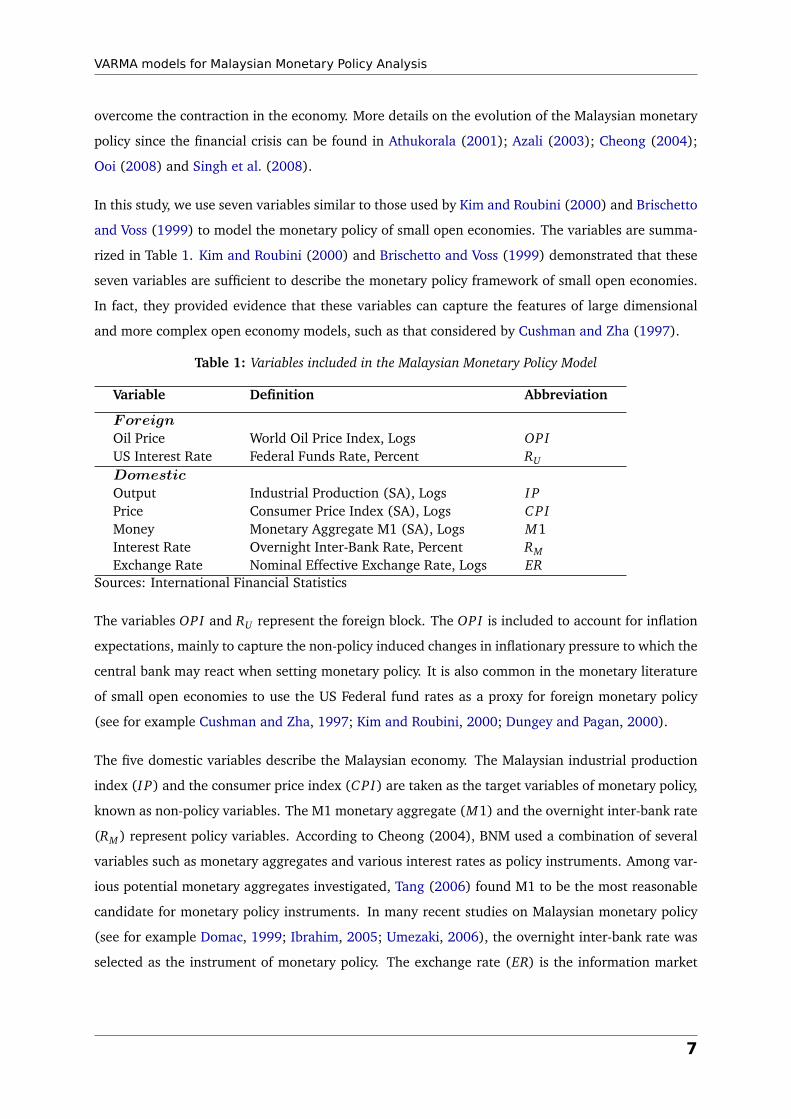
In this study, we use seven variables similar to those used by Kim and Roubini (2000) and Brischetto

and Voss (1999) to model the monetary policy of small open economies. The variables are summa-

rized in Table 1. Kim and Roubini (2000) and Brischetto and Voss (1999) demonstrated that these

seven variables are sufficient to describe the monetary policy framework of small open economies.

In fact, they provided evidence that these variables can capture the features of large dimensional

and more complex open economy models, such as that considered by Cushman and Zha (1997).

Table 1: Variables included in the Malaysian Monetary Policy Model

Variable Definition Abbreviation

ForeignOil Price World Oil Price Index, Logs OPIUS Interest Rate Federal Funds Rate, Percent RU

DomesticOutput Industrial Production (SA), Logs I PPrice Consumer Price Index (SA), Logs C PIMoney Monetary Aggregate M1 (SA), Logs M1Interest Rate Overnight Inter-Bank Rate, Percent RMExchange Rate Nominal Effective Exchange Rate, Logs ER

Sources: International Financial Statistics

The variables OPI and RU represent the foreign block. The OPI is included to account for inflation

expectations, mainly to capture the non-policy induced changes in inflationary pressure to which the

central bank may react when setting monetary policy. It is also common in the monetary literature

of small open economies to use the US Federal fund rates as a proxy for foreign monetary policy

(see for example Cushman and Zha, 1997; Kim and Roubini, 2000; Dungey and Pagan, 2000).

The five domestic variables describe the Malaysian economy. The Malaysian industrial production

index (I P) and the consumer price index (C PI) are taken as the target variables of monetary policy,

known as non-policy variables. The M1 monetary aggregate (M1) and the overnight inter-bank rate

(RM ) represent policy variables. According to Cheong (2004), BNM used a combination of several

variables such as monetary aggregates and various interest rates as policy instruments. Among var-

ious potential monetary aggregates investigated, Tang (2006) found M1 to be the most reasonable

candidate for monetary policy instruments. In many recent studies on Malaysian monetary policy

(see for example Domac, 1999; Ibrahim, 2005; Umezaki, 2006), the overnight inter-bank rate was

selected as the instrument of monetary policy. The exchange rate (ER) is the information market

7


variable. Considering the US dollar peg of the Malaysian Ringgit during the period of study, we em-

ploy the nominal effective exchange rate instead of the bilateral US dollar exchange rate. As stated

by Mehrotra (2005), this trade-weighted exchange rate is believed to capture the movements in the

exchange rate that may have inflationary consequences in the Malaysian economy more compre-

hensively. These five domestic variables are also the standard set of variables used in the monetary

literature to represent open economy monetary business cycle models (see for example Sims, 1992;

Cushman and Zha, 1997; Kim and Roubini, 2000; Christiano et al., 1999).

The sample period of this study is from January 1980 to December 2007. The sample period covers

only the post-liberalization period in Malaysia, which also includes the mid-1997 East Asian financial

crisis. To assess the impact of the financial crisis and the subsequent implementation of capital and

exchange control measures on the Malaysian monetary transmission mechanism, the period of the

study is divided into the pre-crisis period (1980:1 to 1997:6) and the post-crisis period (1999:1 to

2007:12). All data are extracted from the IMF’s International Financial Statistics (IFS) database.

The variables are seasonally adjusted and in logarithms, except for the interest rates, which are

expressed as percentages.

We consider unit root tests for all variables over the whole sample and for both the pre- and post-

crisis periods. Both the Augmented Dickey Fuller and Philips-Perron unit root tests show that all of

the variables are difference stationary over all sample periods. Johansen’s co-integration test also

provides evidence of long run relationships among the seven variables. Given that the variables in

levels are non-stationary and cointegrated, the use of a VAR model in first differences leads to a loss

of information contained in the long run relationships. Since the objective of this study is to assess

the interrelationships between the variables, we concur with Ramaswamy and Sloke (1997) that the

VAR and VARMA in levels remain appropriate measures to correctly identify the effects of monetary

shocks.2

3 Identification and estimation of a VARMA model

For identifying and estimating a VARMA model, we use the Athanasopoulos and Vahid (2008a)

extension of the Tiao and Tsay (1989) scalar component model (SCM) methodology. The aim of

identifying scalar components is to examine whether there are any simplifying embedded structures

underlying a VARMA(p, q) process.

For a given K dimensional VARMA(p, q) process

yt =A1yt−1+ . . .+Apyt−p +υt −M1υt−1− . . .−Mqυt−q, (1)

8


a non-zero linear combination zt =α′yt follows a SCM(p1, q1) ifα satisfies the following properties:

α′Ap16= 0′ where 0≤ p1 ≤ p,

α′Al = 0′ for l = p1+ 1, . . . , p,

α′Mq16= 0′ where 0≤ q1 ≤ q,

α′Ml = 0′ for l = q1+ 1, . . . , q.

The scalar random variable zt depends only on lags 1 to p1 of all variables and lags 1 to q1 of all

innovations in the system. The determination of embedded scalar component models is achieved

through a series of canonical correlation tests.

Denote the estimated squared canonical correlations between Ym,t ≡�

y′t , . . . ,y′t−m

�

and Yh,t−1− j ≡�

y′t−1− j , . . . ,y′t−1− j−h

�′by bλ1 < bλ2 < . . . < bλK . As suggested by Tiao and Tsay (1989), the test

statistic for at least s SCM�

pi , qi�

, i.e., s insignificant canonical correlations, against the alternative

of less than s scalar components is

C (s) =−�

n− h− j�

s∑

i=1

ln

(

1−bλi

di

)

a∼ χ2s×{(h−m)K+s} (2)

where di is a correction factor that accounts for the fact that the canonical variates could be moving

averages of order j, and is calculated as follows:

di = 1+ 2j∑

v=1

bρv

�

br′iYm,t

�

bρv

�

bg′iYh,t−1− j

�

, (3)

where bρv (.) is the v th order autocorrelation of its argument and br′iYm,t and bg′iYh,t−1− j are the

canonical variates corresponding to the i th canonical correlation between Ym,t and Yh,t−1− j . Let

Γ(m, h, j) = E(Yh,t−1− jY′

m,t). This is a sub-matrix of the Hankel matrix of the autocovariance ma-

trices of yt . Note that zero canonical correlations imply and are implied by Γ(m, h, j) having a zero

eigenvalue.

Below, we provide a brief description of the complete VARMA methodology based on scalar

components. For further details, refer to Athanasopoulos and Vahid (2008a) and Tiao and Tsay

(1989).

Stage I: Identifying the scalar components

9


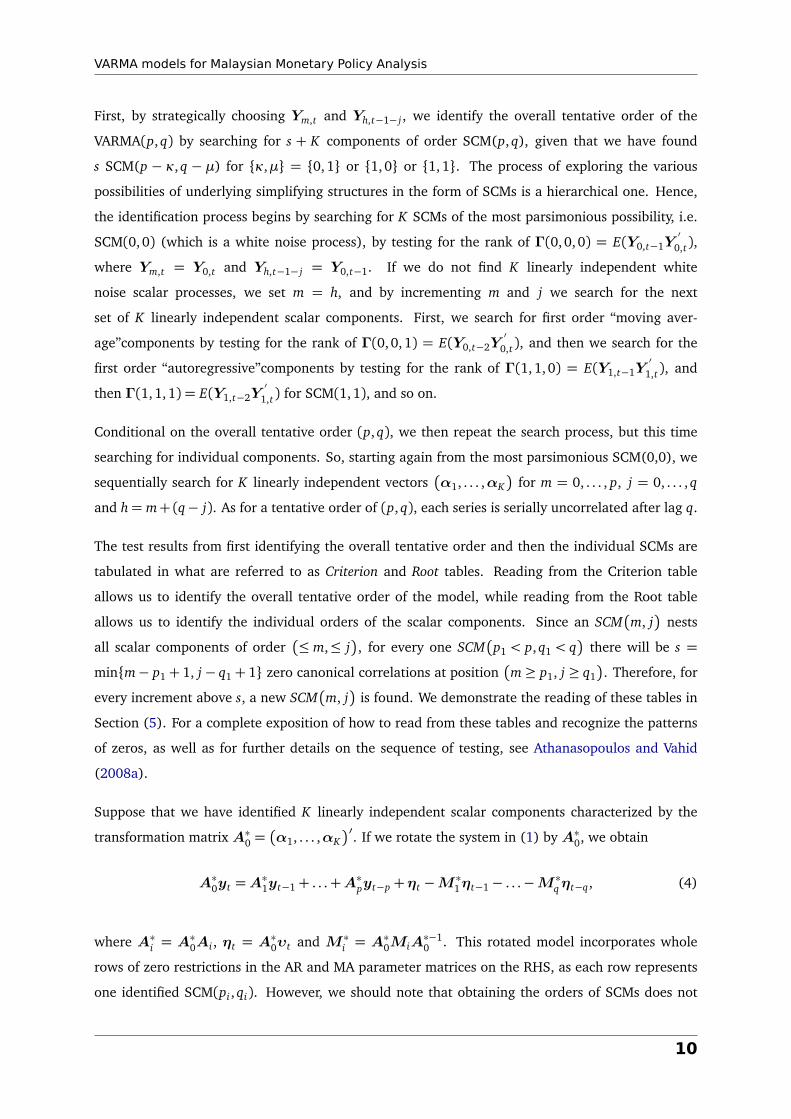
First, by strategically choosing Ym,t and Yh,t−1− j , we identify the overall tentative order of the

VARMA(p, q) by searching for s + K components of order SCM(p, q), given that we have found

s SCM(p − κ, q − µ) for {κ,µ} = {0, 1} or {1, 0} or {1, 1}. The process of exploring the various

possibilities of underlying simplifying structures in the form of SCMs is a hierarchical one. Hence,

the identification process begins by searching for K SCMs of the most parsimonious possibility, i.e.

SCM(0, 0) (which is a white noise process), by testing for the rank of Γ(0, 0,0) = E(Y0,t−1Y′

0,t),

where Ym,t = Y0,t and Yh,t−1− j = Y0,t−1. If we do not find K linearly independent white

noise scalar processes, we set m = h, and by incrementing m and j we search for the next

set of K linearly independent scalar components. First, we search for first order “moving aver-

age”components by testing for the rank of Γ(0,0, 1) = E(Y0,t−2Y′

0,t), and then we search for the

first order “autoregressive”components by testing for the rank of Γ(1,1, 0) = E(Y1,t−1Y′

1,t), and

then Γ(1,1, 1) = E(Y1,t−2Y′

1,t) for SCM(1, 1), and so on.

Conditional on the overall tentative order (p, q), we then repeat the search process, but this time

searching for individual components. So, starting again from the most parsimonious SCM(0,0), we

sequentially search for K linearly independent vectors�

α1, . . . ,αK�

for m = 0, . . . , p, j = 0, . . . , q

and h= m+(q− j). As for a tentative order of (p, q), each series is serially uncorrelated after lag q.

The test results from first identifying the overall tentative order and then the individual SCMs are

tabulated in what are referred to as Criterion and Root tables. Reading from the Criterion table

allows us to identify the overall tentative order of the model, while reading from the Root table

allows us to identify the individual orders of the scalar components. Since an SCM�

m, j�

nests

all scalar components of order�

≤ m,≤ j�

, for every one SCM�

p1 < p, q1 < q�

there will be s =

min{m− p1 + 1, j − q1 + 1} zero canonical correlations at position�

m≥ p1, j ≥ q1�

. Therefore, for

every increment above s, a new SCM�

m, j�

is found. We demonstrate the reading of these tables in

Section (5). For a complete exposition of how to read from these tables and recognize the patterns

of zeros, as well as for further details on the sequence of testing, see Athanasopoulos and Vahid

(2008a).

Suppose that we have identified K linearly independent scalar components characterized by the

transformation matrix A∗0 =�

α1, . . . ,αK�′. If we rotate the system in (1) by A∗0, we obtain

A∗0yt =A∗1yt−1+ . . .+A∗pyt−p +ηt −M ∗

1ηt−1− . . .−M ∗qηt−q, (4)

where A∗i = A∗0Ai , ηt = A∗0υt and M ∗

i = A∗0MiA

∗−10 . This rotated model incorporates whole

rows of zero restrictions in the AR and MA parameter matrices on the RHS, as each row represents

one identified SCM(pi , qi). However, we should note that obtaining the orders of SCMs does not

10


necessarily lead to a uniquely identified system. For example, if two scalar components were

identified such that zr,t = SC M�

pr , qr�

and zs,t = SC M�

ps, qs�

, where pr > ps and qr > qs, the

system will not be identified. To obtain an identified system, we need to set min�

pr − ps, qr − qs

,

i.e. set either the autoregressive or moving average parameters to be zero. This process is known

as the “general rule of elimination”, and in order to identify a canonical VARMA model as defined

by Athanasopoulos and Vahid (2008a), we set the moving average parameters to zero.

Stage II: Imposing identification restrictions on matrix A∗0

Athanasopoulos and Vahid (2008a) recognized that some of the parameters in A∗0 are redundant

and can be eliminated. This stage mainly outlines this process, and a brief description of the rules

of placing restrictions on the redundant parameters is as follows:

1. Given that each row of the transformation matrix A∗0 can be multiplied by a constant without

changing the structure of the model, one parameter in each row can be normalized to one.

However, there is a danger of normalizing the wrong parameter, i.e. a zero parameter might

be normalized to one. To overcome this problem, we add tests of predictability using subsets

of variables. Starting from the SCM with the smallest order (the SCM with minimum p+ q),

exclude one variable, say the K th variable, and test whether a SCM of the same order can

be found using the K − 1 variables alone. If the test is rejected, the coefficient of the K th

variable is then normalised to one, and the corresponding coefficients in all other SCMs that

nest this one are set to zero. If the test concludes that the SCM can be formed using the first

K − 1 variables only, the coefficient of the K th variable in this SCM is zero, and should not

be normalised to one. It is worth noting that if the order of this SCM is uniquely minimal,

then this extra zero restriction adds to the restrictions discovered before. Continue testing by

leaving out variables K −1 and testing whether the SCM could be formed from the first K −2

variables only, and so on.

2. Any linear combination of a SCM�

p1, q1�

and a SCM�

p2, q2�

is a

SCM�

max�

p1, p2

, max�

q1, q2�

. The row of matrix A∗0 corresponding to the SCM�

p1, q1�

is not identified if there are two embedded scalar components with weakly nested orders,

i.e., p1 ≥ p2 and q1 ≥ q2. In this case arbitrary multiples of SCM�

p2, q2�

can be added to

the SCM�

p1, q1�

without changing the structure. To achieve identification, if the parameter

in the i th column of the row of A∗0 corresponding to the SCM�

p2, q2�

is normalized to one,

the parameter in the same position in the row of A∗0 corresponding to SCM�

p1, q1�

should

be restricted to zero. A detailed explanation on this issue, together with an example, can be

found in Athanasopoulos and Vahid (2008a).

11


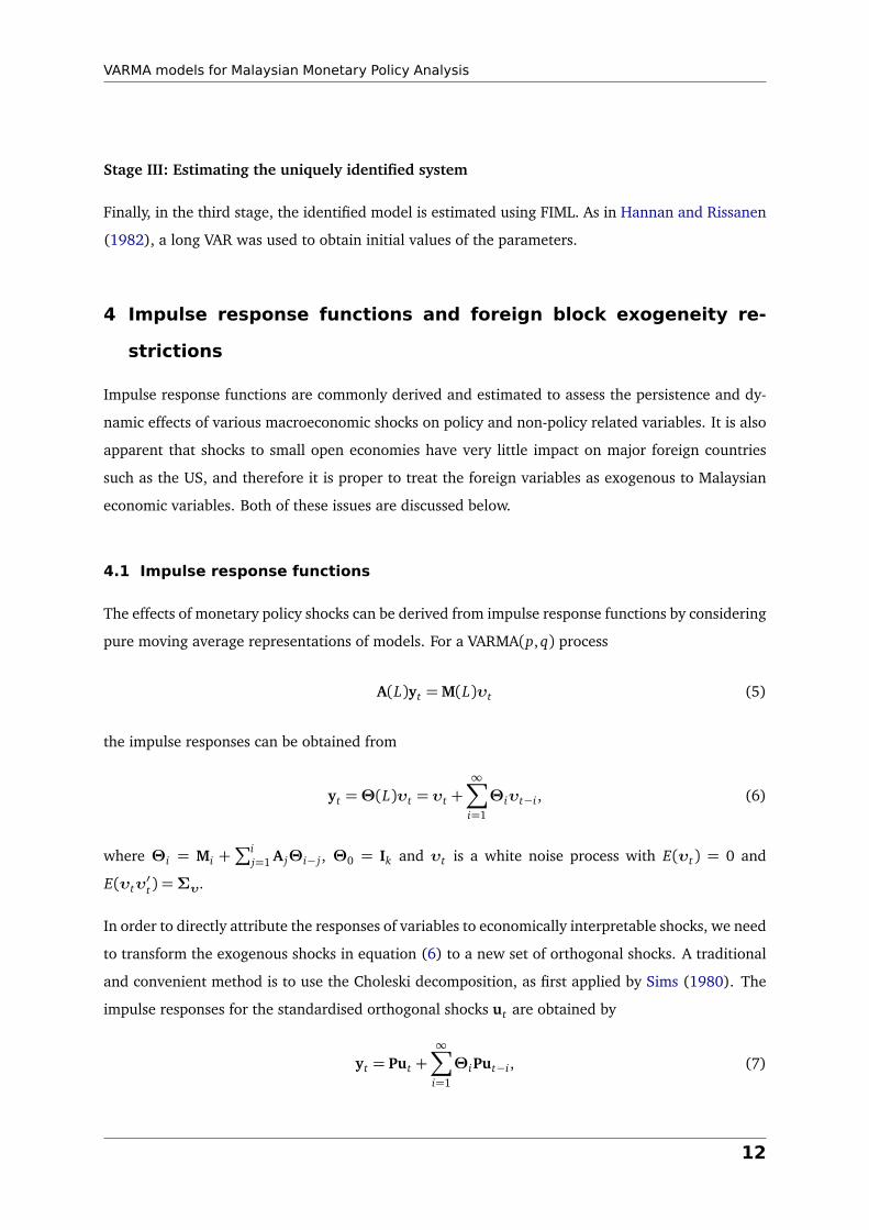
Stage III: Estimating the uniquely identified system

Finally, in the third stage, the identified model is estimated using FIML. As in Hannan and Rissanen

(1982), a long VAR was used to obtain initial values of the parameters.

4 Impulse response functions and foreign block exogeneity re-

strictions

Impulse response functions are commonly derived and estimated to assess the persistence and dy-

namic effects of various macroeconomic shocks on policy and non-policy related variables. It is also

apparent that shocks to small open economies have very little impact on major foreign countries

such as the US, and therefore it is proper to treat the foreign variables as exogenous to Malaysian

economic variables. Both of these issues are discussed below.

4.1 Impulse response functions

The effects of monetary policy shocks can be derived from impulse response functions by considering

pure moving average representations of models. For a VARMA(p, q) process

A(L)yt =M(L)υt (5)

the impulse responses can be obtained from

yt =Θ(L)υt = υt +∞∑

i=1

Θiυt−i , (6)

where Θi = Mi +∑i

j=1 A jΘi− j , Θ0 = Ik and υt is a white noise process with E(υt) = 0 and

E(υtυ′t) =Συ.

In order to directly attribute the responses of variables to economically interpretable shocks, we need

to transform the exogenous shocks in equation (6) to a new set of orthogonal shocks. A traditional

and convenient method is to use the Choleski decomposition, as first applied by Sims (1980). The

impulse responses for the standardised orthogonal shocks ut are obtained by

yt = Put +∞∑

i=1

ΘiPut−i , (7)

12


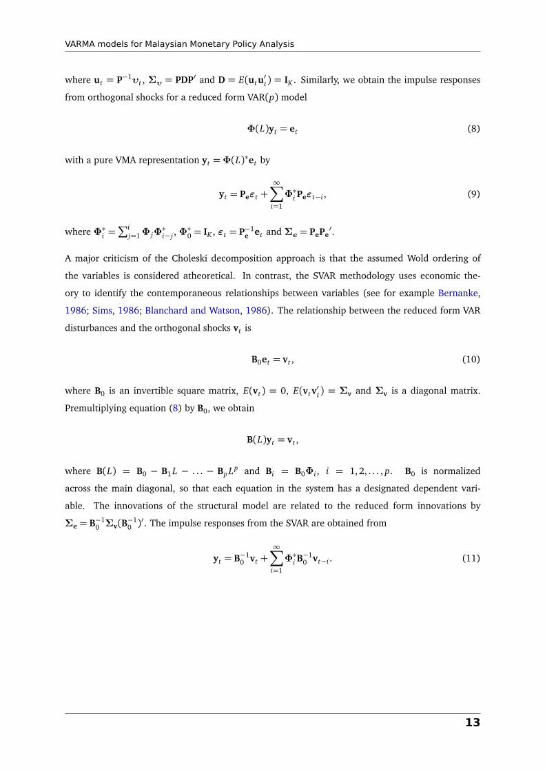
where ut = P−1υt , Συ = PDP′ and D = E(utu′t) = IK . Similarly, we obtain the impulse responses

from orthogonal shocks for a reduced form VAR(p) model

Φ(L)yt = et (8)

with a pure VMA representation yt =Φ(L)∗et by

yt = Peεt +∞∑

i=1

Φ∗i Peεt−i , (9)

where Φ∗i =∑i

j=1 Φ jΦ∗i− j , Φ∗0 = IK , εt = P−1

e et and Σe = PePe′.

A major criticism of the Choleski decomposition approach is that the assumed Wold ordering of

the variables is considered atheoretical. In contrast, the SVAR methodology uses economic the-

ory to identify the contemporaneous relationships between variables (see for example Bernanke,

1986; Sims, 1986; Blanchard and Watson, 1986). The relationship between the reduced form VAR

disturbances and the orthogonal shocks vt is

B0et = vt , (10)

where B0 is an invertible square matrix, E(vt) = 0, E(vtv′t) = Σv and Σv is a diagonal matrix.

Premultiplying equation (8) by B0, we obtain

B(L)yt = vt ,

where B(L) = B0 − B1 L − . . . − Bp Lp and Bi = B0Φi , i = 1,2, . . . , p. B0 is normalized

across the main diagonal, so that each equation in the system has a designated dependent vari-

able. The innovations of the structural model are related to the reduced form innovations by

Σe = B−10 Σv(B

−10 )′. The impulse responses from the SVAR are obtained from

yt = B−10 vt +

∞∑

i=1

Φ∗i B−10 vt−i . (11)

13


Similar to Kim and Roubini (2000) and Brischetto and Voss (1999), we use a non-recursive identifi-

cation structure on the contemporaneous matrix B0. We define

B0 =

1 0 0 0 0 0 0

b021 1 0 0 0 0 0

b031 0 1 0 0 0 0

b041 0 b0

43 1 0 0 0

0 0 b053 b0

54 1 b056 0

b061 b0

62 0 0 b065 1 0

b071 b0

72 b073 b0

74 b075 b0

76 1

(12)

with the variables ordered as in Table 1. Our model differs slightly from Kim and Roubini’s model,

as we allow for the US interest rate to have a contemporaneous impact on domestic monetary policy

by not setting b062 = 0.

4.2 Foreign block exogeneity restrictions

It is sensible to assume that the foreign variables in the Malaysian VARMA, SVAR and VAR systems

are predetermined, and that the domestic variables do not Granger cause the foreign variables

(see for example Cushman and Zha, 1997; Dungey and Pagan, 2000). To impose foreign block

exogeneity, we divide the variables into foreign and domestic blocks, i.e.,

yt = (y1,t ,y2,t)′, (13)

where y1,t = (OPIt , RU ,t) and y2,t = (I Pt , C PIt , M1t , RM ,t , ERt). In all three models, we restrict all

parameters of the domestic variables that enter into the equations of the foreign variables either

contemporaneously or as lagged values to zero. For example, in the VARMA model we set

A(L) =

A11(L) 0

A21(L) A22(L)

and M(L) =

M11(L) 0

M21(L) M22(L).

(14)

Beside the foreign block exogeneity restrictions, no further restrictions are imposed on the lag struc-

tures of the VAR and SVAR models. On the other hand, due to the identification issues discussed

in Section (3), further restrictions are imposed for the VARMA model in order to identify a unique

VARMA process.

14


5 Empirical results

In this section, we apply the complete VARMA methodology outlined in Section (3) to the Malaysian

monetary model of seven variables. The impulse responses generated from the identified VARMA,

VAR and SVAR models for Malaysian monetary policy are then used to assess the effects of various

monetary shocks.

5.1 Specifying VARMA, VAR and SVAR models

In Stage 1, we identify the overall order of the VARMA process and the orders of embedded SCMs

in the data for the pre- and post-crisis periods. In Panel A of Table 2 we report the results of all

canonical correlations test statistics, divided by their χ2 critical values, for the pre-crisis period.

This table is known as the “Criterion Table”. If the entry in the�

m, j�th cell is less than one, this

shows that there are seven SCMs of order�

m, j�

or lower in this system.

From Panel A in Table 2, we infer that the overall order of the system is VARMA(1, 1). Conditional

on this overall order, the canonical correlation tests are employed to identify the individual orders

of embedded SCMs. The number of insignificant canonical correlations identified are tabulated in

Panel B of Table 2, which is referred to as the “Root Table”. In the Root Table, the bold entries show

that one scalar component of order (1,0) is initially identified in position�

m, j�

= (1, 0). Then, there

are seven SCMs of order (1,1) at position�

m, j�

= (1, 1). From these seven, one is carried through

from the previous one (1, 0) scalar component, and the remaining six are new scalar components of

order (1, 1). Hence, the identified VARMA(1, 1) consists of one SCM(1, 0) and six SCM(1,1)s.

Using the identification rules described in Section (3), a canonical SCM representation of the iden-

tified VARMA(1,1) of the Malaysian monetary model for the pre-crisis period is given below, where

yt = (OPI t , RU ,t , I Pt , C PIt , M1t , RM ,t , ERt)′.

Table 2: Stage I of the identification process of a VARMA model for the Malaysian Monetary System forthe pre-crisis period

PANEL A: Criterion Table PANEL B: Root Tablej j

m 0 1 2 3 4 m 0 1 2 3 40 66.41a 6.79 3.51 2.30 1.68 0 0 0 0 1 21 4.33 0.87 0.77 0.91 1.00 1 1 7 7 7 82 1.07 1.11 1.00 0.85 0.92 2 6 9 14 14 143 0.91 0.97 0.96 1.03 0.89 3 7 13 16 20 214 1.15 1.09 0.99 0.98 1.03 4 6 12 20 23 26aThe statistics are normalized by the corresponding 5% χ2critical values

15


1 0 0 0 0 0 0

0 1 0 0 0 0 0

0 0 1 0 0 0 0

0 0 0 1 0 0 0

0 0 0 0 1 0 0

0 0 0 0 0 1 0

0 0 0 0 0 0 1

yt = c+

ψ(1)11 ψ

(1)12 0 0 0 0 0

ψ(1)21 ψ

(1)22 0 0 0 0 0

ψ(1)31 ψ

(1)32 ψ

(1)33 ψ

(1)34 ψ

(1)35 ψ

(1)36 ψ

(1)37

ψ(1)41 ψ

(1)42 ψ

(1)43 ψ

(1)44 ψ

(1)45 ψ

(1)46 ψ

(1)47

ψ(1)51 ψ

(1)52 ψ

(1)53 ψ

(1)54 ψ

(1)55 ψ

(1)56 ψ

(1)57

ψ(1)61 ψ

(1)62 ψ

(1)63 ψ

(1)64 ψ

(1)65 ψ

(1)66 ψ

(1)67

ψ(1)71 ψ

(1)72 ψ

(1)73 ψ

(1)74 ψ

(1)75 ψ

(1)76 ψ

(1)77

yt−1

+ut −

µ(1)11 µ

(1)12 0 0 0 0 0

µ(1)21 µ

(1)22 0 0 0 0 0

µ(1)31 µ

(1)32 µ

(1)33 µ

(1)34 µ

(1)35 µ

(1)36 µ

(1)37

0 0 0 0 0 0 0

µ(1)51 µ

(1)52 µ

(1)53 µ

(1)54 µ

(1)55 µ

(1)56 µ

(1)57

µ(1)61 µ

(1)62 µ

(1)63 µ

(1)64 µ

(1)65 µ

(1)66 µ

(1)67

0µ(1)71 µ(1)72 µ

(1)73 µ

(1)74 µ

(1)75 µ

(1)76 µ

(1)77

ut−1.

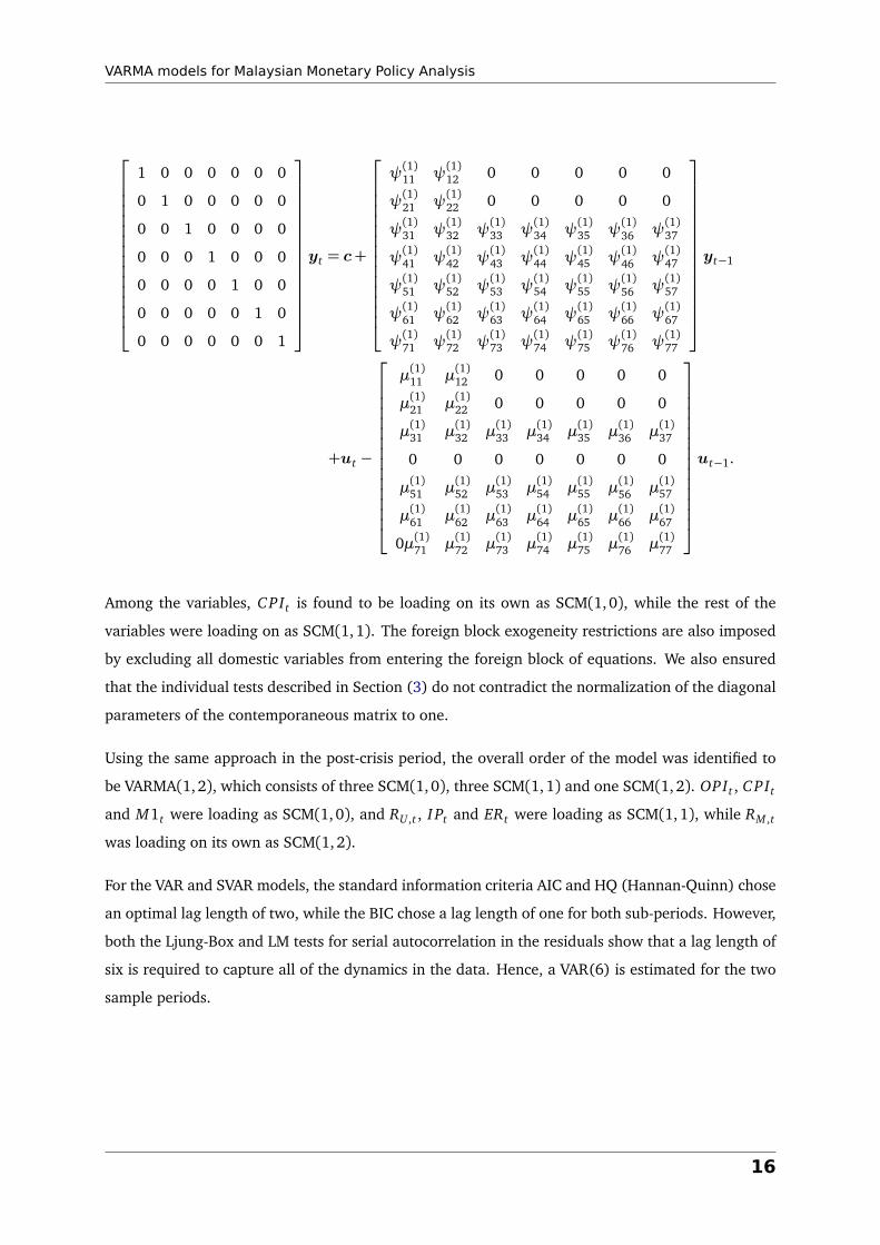
Among the variables, C PIt is found to be loading on its own as SCM(1,0), while the rest of the

variables were loading on as SCM(1, 1). The foreign block exogeneity restrictions are also imposed

by excluding all domestic variables from entering the foreign block of equations. We also ensured

that the individual tests described in Section (3) do not contradict the normalization of the diagonal

parameters of the contemporaneous matrix to one.

Using the same approach in the post-crisis period, the overall order of the model was identified to

be VARMA(1,2), which consists of three SCM(1,0), three SCM(1,1) and one SCM(1, 2). OPIt , C PIt

and M1t were loading as SCM(1,0), and RU ,t , I Pt and ERt were loading as SCM(1,1), while RM ,t

was loading on its own as SCM(1, 2).

For the VAR and SVAR models, the standard information criteria AIC and HQ (Hannan-Quinn) chose

an optimal lag length of two, while the BIC chose a lag length of one for both sub-periods. However,

both the Ljung-Box and LM tests for serial autocorrelation in the residuals show that a lag length of

six is required to capture all of the dynamics in the data. Hence, a VAR(6) is estimated for the two

sample periods.

16


5.2 Responses of domestic variables to various policy shocks

The key impulse response functions of domestic variables to independent shocks, derived from

VARMA, VAR and SVAR specifications, are revealed in Figures 1 to 4 and are discussed in this

section. The sizes of the shocks are measured by one-standard deviation of the orthogonal errors

of the respective models. Broadly speaking, a comparison of the results of the three alternative

models for the pre- and post-crisis periods indicates the benefits of using the VARMA model over its

VAR/SVAR counterparts. Furthermore, the VARMA model performs much better than the other two

models in cases that matters to policymakers, particularly in the post-crisis period. Therefore, we

say at the outset that the discussions that follow are based largely on VARMA models.

Responses to a foreign monetary policy shock

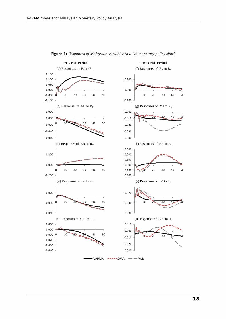
The responses of domestic variables to a RU shock are shown in Figure 1 for the pre- and post-1997

crisis periods, and we first discuss the results for the pre-crisis period: an increase in RM , as expected

under a controlled exchange rate system with unrestricted capital flows - a regime Malaysia pursued

over this period. This positive response of RM caused a decline in M1. Furthermore, the Ringgit

(ER) depreciated mildly as both a direct response to the RU shock and an opposite reaction to the

increase in RM , which is only revealed by the VARMA model. This is also partly due to an attempt

to lean against the nominal exchange rate depreciation, especially under a managed exchange

rate regime. The combined effects of an increase in RM and a largely insensitive exchange rate

subsequently triggered a decline in both I P and C PI nearly a year later. For the post-crisis period,

on the other hand, the responses of RM , M1, I P and C PI to a RU shock are the same as those for the

pre-crisis period, although the changes are all less prominent. Moreover, as indicated only by the

VARMA model, the Ringgit has slightly appreciated. While Malaysia has pegged its currency to the

US dollar and introduced capital control measures in an effort to regain its monetary independence,

the rise in RM and the fall in M1 are indications that the country has not experienced absolute

monetary autonomy under the fixed exchange rate regime. However, it is apparent from the mild

effects on I P and C PI that the stringent capital control measures that Malaysia imposed have

helped to insulate the economy to some extent from foreign monetary shocks.

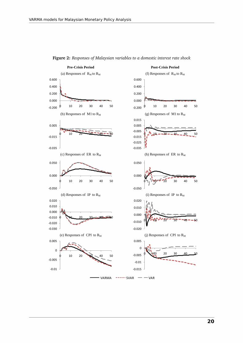
Responses to a domestic monetary policy shock

Shocks to RM are treated as changes to monetary policy. The responses of the domestic variables

to a RM shock are shown in Figure 2: a short-run increase in RM , itself lasting for a year. In the

pre-crisis period, M1 declined – with the effect accentuated by the VARMA model – ER appreciated,

as influenced by market forces, and I P and C PI contracted. The sluggish response of C PI signals

17


Figure 1: Responses of Malaysian variables to a US monetary policy shock

Pre-Crisis Period Post-Crisis Period

(a) Responses of RM to RU (f) Responses of RM to RU

(b) Responses of M1 to RU (g) Responses of M1 to RU

(c) Responses of ER to RU (h) Responses of ER to RU

(d) Responses of IP to RU (i) Responses of IP to RU

(e) Responses of CPI to RU (j) Responses of CPI to RU

-0.100

-0.050

0.000

0.050

0.100

0.150

0 10 20 30 40 50

-0.100

0.000

0.100

0 10 20 30 40 50

-0.060

-0.040

-0.020

0.000

0.020

0 10 20 30 40 50

-0.040

-0.030

-0.020

-0.010

0.000

0 10 20 30 40 50

-0.200

0.000

0.200

0 10 20 30 40 50

-0.200

-0.100

0.000

0.100

0.200

0.300

0 10 20 30 40 50

-0.080

-0.030

0.020

0 10 20 30 40 50

-0.080

-0.030

0.020

0 10 20 30 40 50

-0.040

-0.030

-0.020

-0.010

0.000

0.010

0 10 20 30 40 50

-0.030

-0.020

-0.010

0.000

0.010

0 10 20 30 40 50

-0.06

-0.04

-0.02

0

0.02

0.04

0.06

1 11 21 31 41 51

VARMA SVAR VAR

18


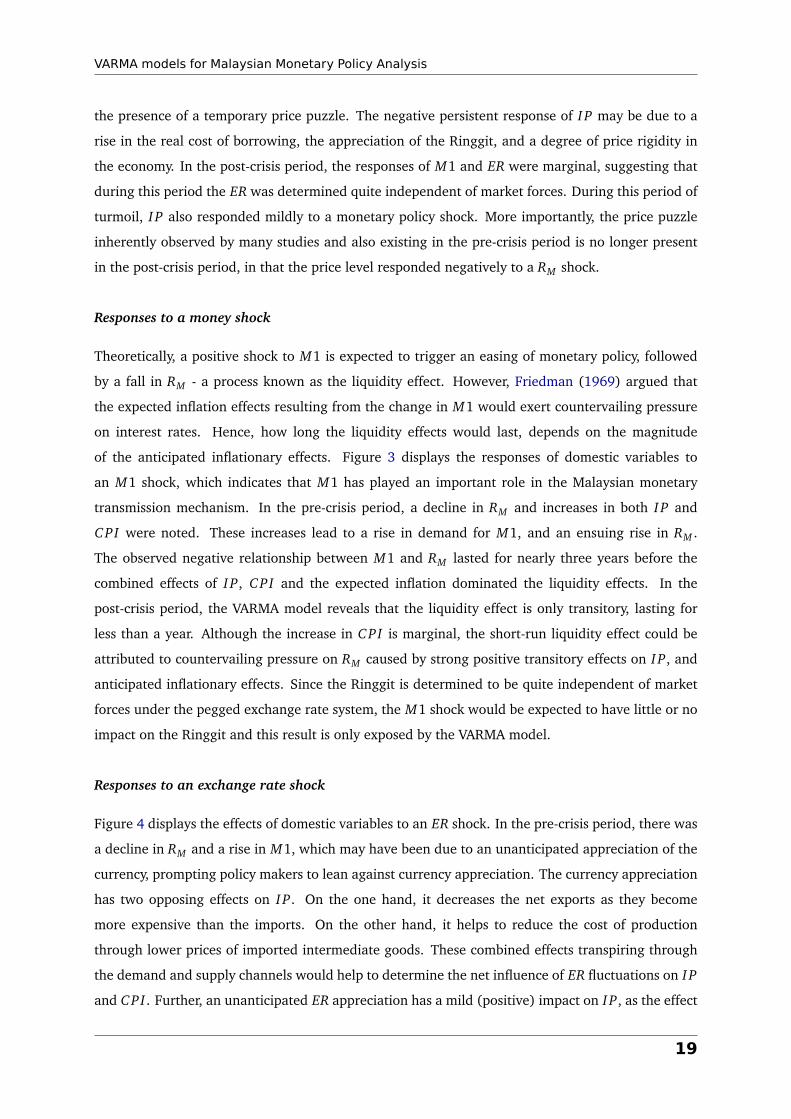
the presence of a temporary price puzzle. The negative persistent response of I P may be due to a

rise in the real cost of borrowing, the appreciation of the Ringgit, and a degree of price rigidity in

the economy. In the post-crisis period, the responses of M1 and ER were marginal, suggesting that

during this period the ER was determined quite independent of market forces. During this period of

turmoil, I P also responded mildly to a monetary policy shock. More importantly, the price puzzle

inherently observed by many studies and also existing in the pre-crisis period is no longer present

in the post-crisis period, in that the price level responded negatively to a RM shock.

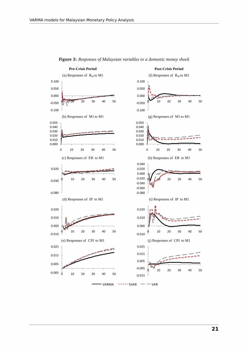
Responses to a money shock

Theoretically, a positive shock to M1 is expected to trigger an easing of monetary policy, followed

by a fall in RM - a process known as the liquidity effect. However, Friedman (1969) argued that

the expected inflation effects resulting from the change in M1 would exert countervailing pressure

on interest rates. Hence, how long the liquidity effects would last, depends on the magnitude

of the anticipated inflationary effects. Figure 3 displays the responses of domestic variables to

an M1 shock, which indicates that M1 has played an important role in the Malaysian monetary

transmission mechanism. In the pre-crisis period, a decline in RM and increases in both I P and

C PI were noted. These increases lead to a rise in demand for M1, and an ensuing rise in RM .

The observed negative relationship between M1 and RM lasted for nearly three years before the

combined effects of I P, C PI and the expected inflation dominated the liquidity effects. In the

post-crisis period, the VARMA model reveals that the liquidity effect is only transitory, lasting for

less than a year. Although the increase in C PI is marginal, the short-run liquidity effect could be

attributed to countervailing pressure on RM caused by strong positive transitory effects on I P, and

anticipated inflationary effects. Since the Ringgit is determined to be quite independent of market

forces under the pegged exchange rate system, the M1 shock would be expected to have little or no

impact on the Ringgit and this result is only exposed by the VARMA model.

Responses to an exchange rate shock

Figure 4 displays the effects of domestic variables to an ER shock. In the pre-crisis period, there was

a decline in RM and a rise in M1, which may have been due to an unanticipated appreciation of the

currency, prompting policy makers to lean against currency appreciation. The currency appreciation

has two opposing effects on I P. On the one hand, it decreases the net exports as they become

more expensive than the imports. On the other hand, it helps to reduce the cost of production

through lower prices of imported intermediate goods. These combined effects transpiring through

the demand and supply channels would help to determine the net influence of ER fluctuations on I P

and C PI . Further, an unanticipated ER appreciation has a mild (positive) impact on I P, as the effect

19


Figure 2: Responses of Malaysian variables to a domestic interest rate shock


(a) Responses of RM to RM (f) Responses of RM to RM

(b) Responses of M1 to RM (g) Responses of M1 to RM

(c) Responses of ER to RM (h) Responses of ER to RM

(d) Responses of IP to RM (i) Responses of IP to RM

(e) Responses of CPI to RM (j) Responses of CPI to RM

-0.200

0.000

0.200

0.400

0.600

0 10 20 30 40 50-0.200

0.000

0.200

0.400

0.600

0 10 20 30 40 50

-0.035

-0.015

0.005

0 10 20 30 40 50

-0.035

-0.025

-0.015

-0.005

0.005

0.015

0 10 20 30 40 50

-0.050

0.000

0.050

0 10 20 30 40 50

-0.050

0.000

0.050

0 10 20 30 40 50

-0.030

-0.020

-0.010

0.000

0.010

0.020

0 10 20 30 40 50

-0.020

-0.010

0.000

0.010

0.020

0 10 20 30 40 50

-0.01

-0.005

0

0.005

0 10 20 30 40 50

-0.015

-0.01

-0.005

0

0.005

0 10 20 30 40 50

-0.06

-0.04

-0.02

0

0.02

0.04

0.06

1 11 21 31 41 51

VARMA SVAR VAR

20


Figure 3: Responses of Malaysian variables to a domestic money shock


(a) Responses of RM to M1 (f) Responses of RM to M1

(b) Responses of M1 to M1 (g) Responses of M1 to M1

(c) Responses of ER to M1 (h) Responses of ER to M1

(d) Responses of IP to M1 (i) Responses of IP to M1

(e) Responses of CPI to M1 (j) Responses of CPI to M1

-0.100

-0.050

0.000

0.050

0.100

0 10 20 30 40 50

-0.100

-0.050

0.000

0.050

0.100

0 10 20 30 40 50

0.000

0.010

0.020

0.030

0.040

0.050

0 10 20 30 40 50

0.000

0.010

0.020

0.030

0.040

0.050

0 10 20 30 40 50

-0.080

-0.030

0.020

0 10 20 30 40 50

-0.080

-0.060

-0.040

-0.020

0.000

0.020

0.040

0 10 20 30 40 50

-0.010

0.000

0.010

0.020

0 10 20 30 40 50-0.010

0.000

0.010

0.020

0 10 20 30 40 50

-0.005

0.005

0.015

0.025

0 10 20 30 40 50 -0.015

-0.005

0.005

0.015

0.025

0 10 20 30 40 50

-0.06

-0.04

-0.02

0

0.02

0.04

0.06

1 11 21 31 41 51

VARMA SVAR VAR

21


of a fall in production costs may be offset by the fall in net exports, while at the same time it has

a negative effect on C PI , which could be attributed to both the decline in production costs and the

prices of imported goods. In the post-crisis period, RM declined, but the size of the fall was smaller

than for the pre-crisis period. I P also declined, implying that the fall in net exports outweighed the

benefits of the reduced production costs during this period. Overall, in the post-crisis period, we find

that the VARMA model has uncovered more consistent results than its VAR or SVAR counterparts as

to the way in which domestic variables respond dynamically to ER shocks.

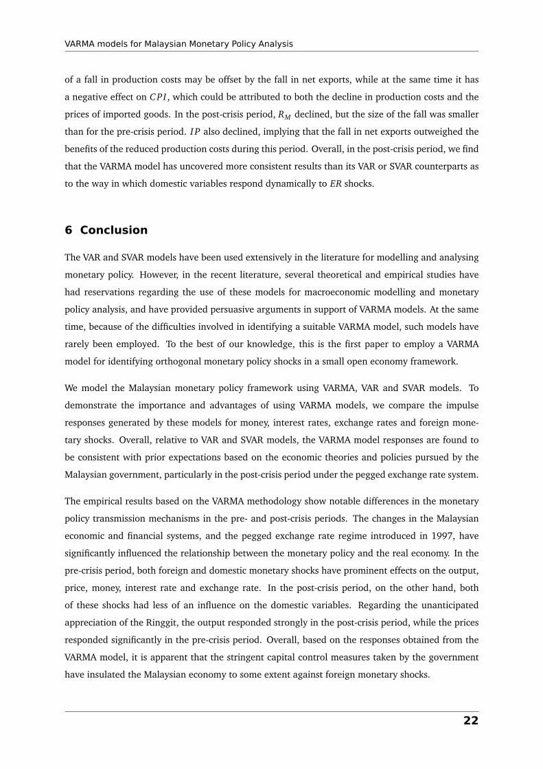
6 Conclusion

The VAR and SVAR models have been used extensively in the literature for modelling and analysing

monetary policy. However, in the recent literature, several theoretical and empirical studies have

had reservations regarding the use of these models for macroeconomic modelling and monetary

policy analysis, and have provided persuasive arguments in support of VARMA models. At the same

time, because of the difficulties involved in identifying a suitable VARMA model, such models have

rarely been employed. To the best of our knowledge, this is the first paper to employ a VARMA

model for identifying orthogonal monetary policy shocks in a small open economy framework.

We model the Malaysian monetary policy framework using VARMA, VAR and SVAR models. To

demonstrate the importance and advantages of using VARMA models, we compare the impulse

responses generated by these models for money, interest rates, exchange rates and foreign mone-

tary shocks. Overall, relative to VAR and SVAR models, the VARMA model responses are found to

be consistent with prior expectations based on the economic theories and policies pursued by the

Malaysian government, particularly in the post-crisis period under the pegged exchange rate system.

The empirical results based on the VARMA methodology show notable differences in the monetary

policy transmission mechanisms in the pre- and post-crisis periods. The changes in the Malaysian

economic and financial systems, and the pegged exchange rate regime introduced in 1997, have

significantly influenced the relationship between the monetary policy and the real economy. In the

pre-crisis period, both foreign and domestic monetary shocks have prominent effects on the output,

price, money, interest rate and exchange rate. In the post-crisis period, on the other hand, both

of these shocks had less of an influence on the domestic variables. Regarding the unanticipated

appreciation of the Ringgit, the output responded strongly in the post-crisis period, while the prices

responded significantly in the pre-crisis period. Overall, based on the responses obtained from the

VARMA model, it is apparent that the stringent capital control measures taken by the government

have insulated the Malaysian economy to some extent against foreign monetary shocks.

22


Figure 4: Responses of Malaysian variables to a domestic exchange rate shock


(a) Responses of RM to ER (f) Responses of RM to ER

(b) Responses of M1 to ER (g) Responses of M1 to ER

(c) Responses of ER to ER (h) Responses of ER to ER

(d) Responses of IP to ER (i) Responses of IP to ER

(e) Responses of CPI to ER (j) Responses of CPI to ER

-0.080

-0.030

0.020

0 10 20 30 40 50

-0.080

-0.030

0.020

0 10 20 30 40 50

-0.002

0

0.002

0.004

0.006

0.008

0.01

0 10 20 30 40 50 -0.015

-0.01

-0.005

0

0.005

0 10 20 30 40 50

0.000

0.050

0.100

0.150

0.200

0.250

0 10 20 30 40 50 -0.050

0.000

0.050

0.100

0.150

0.200

0.250

0 10 20 30 40 50

-0.030

-0.020

-0.010

0.000

0 10 20 30 40 50

-0.030

-0.020

-0.010

0.000

0 20 40 60

-0.01

-0.005

2E-17

0.005

0.01

0.015

0 10 20 30 40 50

-0.01

-0.005

0

0.005

0.01

0.015

0 10 20 30 40 50

-0.06

-0.04

-0.02

0

0.02

0.04

0.06

1 11 21 31 41 51

VARMA SVAR VAR

23


Considering some disparities in the effects of monetary policy on the Malaysian economy during the

pre- and post-crisis periods, it is indispensable for policymakers to understand how the economic

transformation, the openness of the economy and the growing integration with external economies

affect the nature of the monetary transmission mechanism. This study investigates these features

of the Malaysian economy and uncovers the key issues that have implications for the conduct of

monetary policy. In addition, uncovering how various transmission channels work, can help BNM to

steer the economy in the right direction with an appropriate pressure, so that monetary policy can

still remain an effective policy measure in achieving sustainable economic growth and price stability.

Notes

1Economic puzzles are referred to as liquidity puzzles (an unanticipated increase in money supply causes interest rates

to rise instead of falling), price puzzles (an unanticipated tightening of monetary policy causes prices to increase instead

of falling), and exchange rates puzzles (an unanticipated increase in interest rates causes exchange rates to depreciate

instead of appreciating).

2The choice between a VAR in levels (unrestricted VAR) and a VECM (restricted VAR) depends on the economic

interpretation attached to impulse response functions from the two specifications (see Ramaswamy and Sloke, 1997, for

details). The impulse response functions generated from VECM models tend to imply that the impact of monetary shocks

is permanent, while the unrestricted VAR allows the data series to decide whether the effects of the monetary shocks are

permanent or temporary. It is also common in the monetary literature to estimate the unrestricted VAR model in levels

(see for example Sims, 1992; Cushman and Zha, 1997; Bernanke and Mihov, 1998).

References

Athanasopoulos, G. (2007) Essays on alternative methods of identification and estimation of vector

autoregressive moving average models, Ph.D. thesis, Department of Econometrics and Business

Statistics, Monash University, Australia.

Athanasopoulos, G., D. S. Poskitt and F. Vahid (2007) Two canonical VARMA forms: Scalar compo-

nent models vis-à-vis the Echelon form, Working Paper 10-07, Monash University, Australia.

Athanasopoulos, G. and F. Vahid (2008a) A complete VARMA modelling methodology based on

scalar components, Journal of Time Series Analysis, 29, 533–554.

Athanasopoulos, G. and F. Vahid (2008b) VARMA versus VAR for macroeconomic forecasting, Jour-

nal of Business and Economic Statistics, 26, 2.

Athukorala, P. C. (2001) Crisis and recovery in Malaysia: The role of capital controls, Cheltenham:

24


Edward Elgar.

Awang, A. H., T. H. Ng and A. Razi (1992) Financial liberalisation and interest rate determination

in Malaysia, Bank Negara Malaysia.

Azali, M. (2003) Transmission mechanism in a developing economy: Does money or credit matter?,

Second Ed, UPM, Press.

Bernanke, B. S. (1986) Alternative explanations of the money-income correlations, Carnegie-

Rochester Conference Series on Public Policy, 25, 49–99.

Bernanke, B. S. and I. Mihov (1998) Measuring monetary policy, The Quarterly Journal of Economics,

113 (3), 869–902.

Blanchard, O. J. and M. W. Watson (1986) Are business cycles all alike?, in R. Gordon (ed.) The

American Business Cycle: Continuity and Change, pp. 123–156, University of Chicago Press.

Brischetto, A. and G. Voss (1999) A structural vector autoregression model of monetary policy in

Australia, Research Discussion Paper, Reserve Bank of Australia.

Chari, V. V., P. J. Kehoe and E. R. McGrattan (2007) Are structural VARs with long-run restrictions

useful in developing business cycle theory?, Federal Reserve Bank of Minneapolis, Research Depart-

ment Staff Report 364.

Cheong, L. M. (2004) Globalisation and the operation of monetary policy in Malaysia, BIS Papers

No. 23, Bank of International Settlements, 23, 209–215.

Christiano, L. J., M. Eichenbaum and C. L. Evans (1999) Monetary policy shocks: What have we

learned and to what end, chap. 2, Elsevier Science, Amsterdam.

Cooley, T. and M. Dwyer (1998) Business cycle analysis without much theory. A look at structural

VARs, Journal of Econometrics, 83, 57–88.

Cushman, D. O. and T. A. Zha (1997) Identifying monetary policy in a small open economy under

flexible exchange rates, Journal of Monetary Economics, 39, 433–448.

Dekle, R. and M. Pradhan (1997) Financial liberalization and money demand in ASEAN countries:

Implications for monetary policy, IMF Working Paper, WP/97/36.

Domac, I. (1999) The distributional consequences of monetary policy: Evidence from Malaysia,

World Bank Policy Research Working Papers 2170.

Dungey, M. and A. Pagan (2000) A structural VAR model of the Australian economy, The Economic

Record, 76 (235), 321–342.

25


Durbin, J. (1963) Maximum likelihood estimation of the parameters of a system of simultaneous

regression equations, Paper presented to the Copenhagen Meeting of the Econometric Society,

reprinted in Econometric Theory, 4 , 159-170, 1988.

Fernández-Villaverde, J., J. F. Rubio-Ramírez and T. J. Sargent (2005) A,B,C’s (and D’s) for under-

standing VARs, NBER Technical Report 308.

Friedman, M. (1969) Factors affecting the level of interest rates, Proceedings of the 1969 Conference

on Savings and Residential Financing, pp. 11–27.

Fry, R. and A. Pagan (2005) Some issues in using VARs for macroeconometric research, CAMA

Working Paper Series 19/2005, Australian National University.

Granger, C. W. J. and M. J. Morris (1976) Time series modelling interpretation, Journal of the Royal

Statistical Society, 139 (2), 246–257.

Hannan, E. J. and M. Deistler (1988) The statistical theory of linear systems, John Wiley & Sons, New

York.

Hannan, E. J. and J. Rissanen (1982) Recursive estimation of autoregressive-moving average order,

Biometrica, 69, 81–94.

Ibrahim, M. (2005) Sectoral effects on monetary policy: Evidence from Malaysia, Asian Economic

Journal, 19, 83–102.

Kapetanios, G., A. Pagan and A. Scott (2007) Making a match: combining theory and evidence in

policy-oriented macroeconomic modelling, Journal of Econometrics, 136, 565–594.

Kim, S. and N. Roubini (2000) Exchange rate anomalies in the industrial countries: A solution with

a structural VAR approach, Journal of Monetary Economics, 45, 561–586.

Leeper, E. M., C. A. Sims and T. Zha (1996) What does monetary policy do?, Brookings Papers on

Economic Activity 2 ABI/INFORM Global, Federal Reserve Bank of Atlanta.

Lütkepohl, H. (2005) The new introduction to multiple time series analysis, Springer-Verlag, Berlin.

Maravall, A. (1993) Stochastic linear trends: Models and estimators, Journal of Econometrics, 56,

5–37.

McCauley, R. N. (2006) Understanding monetary policy in Malaysia and Thailand: Objectives, in-

struments and independence, BIS Papers No. 31, Bank of International Settlements, pp. 172–198.

Mehrotra, A. (2005) Exchange and interest rate channels during a deflationary era – evidence from

Japan, Hong Kong and China, Discussion Paper (BOFIT).

26


Ooi, S. (2008) The monetary transmission mechanism in Malaysia: Current developments and is-

sues, Bank of International Settlement.

Ramaswamy, R. and T. Sloke (1997) The real effects of monetary policy in the European Union:

What are the differences?, IMF Working Paper, WP/97/160.

Reinsel, G. C. (1997) Elements of multivariate time series, New York: Springer-Verlag, 2nd ed.

Sims, C. A. (1980) Macroeconomics and reality, Econometrica, 48, 1–48.

Sims, C. A. (1986) Are forecasting models useful for policy analysis?

Sims, C. A. (1992) Interpreting the macroeconomic time series facts: The effects of monetary policy,

European Economic Review, 36, 975–1000.

Singh, S., A. Razi, N. Endut and H. Ramlee (2008) Impact of financial market developments on the

monetary transmission mechanism, Bank of International Settlement, 39, 49–99.

Tang, H. C. (2006) The relative importance of monetary policy transmission channels in Malaysia,

CAMA Working Paper Series 23/2006, Australian National University.

Tiao, G. C. and R. S. Tsay (1989) Model specification in multivariate time series, Journal of Royal

Statistical Society, Series B (Methodological), 51 (2), 157–213.

Tseng, W. and R. Corker (1991) Financial liberalization, money demand, monetary policy in Asian

countries, Occasional Paper No. 84, International Monetary Fund.

Umezaki, S. (2006) Monetary and exchange rate policy in Malaysia before the Asian crisis, Discussion

Paper No. 79, Institute of Developing Economies.

Wallis, K. F. (1977) Multiple time series and the final form of econometric models, Econometrica, 45,

1481–1497.

Wold, H. (1938) A study in the analysis of stationary time series, Stockholm: Almqvist and Wiksell.

Zellner, A. and F. Palm (1974) Time series analysis and simultaneous equation econometric models,

Journal of Econometrics, 2, 17–54.

27

Documents

VARMA models for Malaysian Monetary Policy Analysis