Embed Size (px)
Citation preview

Versuchsanstalt für WasserbauHydrologie und Glaziologie
der EidgenössischenTechnischen Hochschule Zürich
Mitteilungen 183
Zürich, 2004
Herausgeber: Prof. Dr.-Ing. H.-E. Minor
Kristian Kramer
Development of Aerated Chute Flow

Herausgeber:Prof. Dr.--Ing. Hans--Erwin Minor
Im Eigenverlag derVersuchsanstalt für Wasserbau,Hydrologie und GlaziologieETH--ZentrumCH--8092 Zürich
Tel.: +41 -- 1 -- 632 4091Fax: +41 -- 1 -- 632 1192e--mail: [email protected]
Zürich, 2004
ISSN 0374--0056

Development of Aerated Chute Flow
i
PREFACE
It has been known for decades that spillway chutes or tailrace channels of
bottom outlets may suffer from cavitation damage if flow velocities are high or
if abrupt changes in flow direction occur. With flow velocities above 30 m/s,
small unavoidable surface imperfections are sufficient to trigger such damage.
The technically most simple and most economic method to avoid cavitation
damage in such conditions is air supply at the contact surface between the
concrete and the water flow. In 1953, Peterka demonstrated with simple tests
that the mass carried away from a test surface is reduced considerably, if 5 % –
8 % air is added to the water. His indications are based on average air
concentration values.
It took until the early eighties of the last century and it needed the large
damage of the spillway chute of the 200 m high Karun arch dam in Iran until
bottom aerators were systematically developed for highly charged spillways.
VAW of ETH Zürich was one of the institutes to develop the design criteria. In
the Western world the focus was air entrainment. Bottom aerators were
optimised to entrain as much air as possible into the high-speed flow.
Concerning air detrainment, everybody relied on poorly documented
publications (which had a lot to do with the language) of Russian authors who
stated that the average air concentration is reduced by 0.4 % – 0.5 % per meter
chute length, due to the air bubble rise. The projects built on the basis of this
assumption, e.g. Foz do Areia in Brazil or Alicura in Argentina, showed that
more air was present in the spillway chute than anticipated. For some projects,
aeration devices were partly closed on purpose, therefore.
Simple analyses of average air concentration along prototype chutes led to
an air detrainment of 0.15 % – 0.20 % per meter chute length. The influences of
parameters like the Froude number or the bottom slope remained unknown.
Here, Kristian Kramer started with his work: He studied the development of
air concentration distribution over the water depth in a straight model flume. Its
slope was adjustable between 0 % and 50 % and, therefore, allowed to study the
influence of the bottom slope. These detailed studies were possible mainly
because novel measuring techniques were available. Kristian Kramer used the

ii
fiber optic measuring system that was previously employed for investigations
on stepped spillways. This system allows measuring the local air concentration,
the flow velocity, and the bubble size.
Kristian Kramer presents some astonishing results. The air entrainment at
the lower side of the jet downstream of a deflector was large, however, shortly
downstream of its point of impact most of the entrained air detrains. The
measured air concentrations at the chute bottom were much lower than those
stated by Peterka. But still we know that in these cases, no cavitation damage
occurred. Kristian Kramer shows also that the air entrainement mechanism
influences the detrainment process. Using his results fairly accurate estimates
can be made on the average air transport in a chute flow. The design procedure
is illustrated with an example.
The research project was funded to a large extent by the Swiss National
Science Foundation for which I am grateful. Furthermore, I owe thanks to
Prof. Dr. W.H. Hager who was guiding the work as co-examiner, as well as
Prof. Dr. H. Kobus, University of Stuttgart, who served as the external
co-examiner.
Zurich, March 2004 Prof. Dr.-Ing. H.-E. Minor

Development of Aerated Chute Flow
iii
ACKNOWLEDGMENTS
This work was carried out during my time as a PhD student and assistant at the
Laboratory of Hydraulics, Hydrology and Glaciology (VAW), ETH Zürich. I
would like to thank all persons who supported me at VAW and contributed in
any form to my thesis, in particular:
Thank you to Prof. Dr.-Ing. H.-E. Minor, for supervising this project, for his
enormous interest and contribution using his wide practical experience. He
enabled this thesis and provided an excellent research environment.
My deepest thanks to Prof. Dr. W.H. Hager who initiated this project and
supported me during my time at VAW. I very much appreciated his advice and
corrections, far exceeding the self-evident.
I would also like to thank Prof. Dr. H. Kobus for thoroughly reviewing this
thesis and being the external co-examiner.
Further, I would like to thank my office companions and colleagues for
giving me a good time at VAW. Thank you for the motivation, support and
discussions in hydraulics and other fields of interest.
I am grateful to the VAW workshop, the electronics workshop, the drawers,
the photographer, the secretaries and my diploma students for supporting me
with all their means.
This thesis profited from suggestions and discussions with Dr.-
Ing. H. Falvey and Prof. Dr. A. Ervine.
Thank you to Silviana and Michael for reading the draft. This research
project was supported by the Swiss National Science Foundation (Project No.
2100-057081.99/1) and the Swiss Committee on Dams.
Very many thanks to my family and friends for their support, considerations
and patience during my time being a PhD student.

iv

Development of Aerated Chute Flow
v
CONTENTS
Acknowledgments . . . . . . . . . . . . . . . . . . . . . . . . . . . . . . . . . . . . . . . . . . . . . . . . . . . iii
Contents . . . . . . . . . . . . . . . . . . . . . . . . . . . . . . . . . . . . . . . . . . . . . . . . . . . . . . . . . . . . v
Abstract . . . . . . . . . . . . . . . . . . . . . . . . . . . . . . . . . . . . . . . . . . . . . . . . . . . . . . . . . . . ix
Kurzfassung . . . . . . . . . . . . . . . . . . . . . . . . . . . . . . . . . . . . . . . . . . . . . . . . . . . . . . . . xi
Chapter 1 Introduction 1
1.1 Problem outline . . . . . . . . . . . . . . . . . . . . . . . . . . . . . . . . . . . . . . . . . . . . . . 11.2 Purpose and aim of present studies . . . . . . . . . . . . . . . . . . . . . . . . . . . . . . . 31.3 Overview . . . . . . . . . . . . . . . . . . . . . . . . . . . . . . . . . . . . . . . . . . . . . . . . . . . 4
Chapter 2 L iterature review 5
2.1 Introduction . . . . . . . . . . . . . . . . . . . . . . . . . . . . . . . . . . . . . . . . . . . . . . . . . 52.2 Cavitation on chutes . . . . . . . . . . . . . . . . . . . . . . . . . . . . . . . . . . . . . . . . . . 5
2.2.1 Cavitation formation . . . . . . . . . . . . . . . . . . . . . . . . . . . . . . . . . . . . . . . . 52.2.2 Cavitation damage . . . . . . . . . . . . . . . . . . . . . . . . . . . . . . . . . . . . . . . . . . 6
2.3 Methods to reduce cavitation damage . . . . . . . . . . . . . . . . . . . . . . . . . . . . 102.3.1 General methods . . . . . . . . . . . . . . . . . . . . . . . . . . . . . . . . . . . . . . . . . . 102.3.2 Effect of air content . . . . . . . . . . . . . . . . . . . . . . . . . . . . . . . . . . . . . . . . 11
2.4 Air entrainment on chutes . . . . . . . . . . . . . . . . . . . . . . . . . . . . . . . . . . . . . 152.4.1 Introduction . . . . . . . . . . . . . . . . . . . . . . . . . . . . . . . . . . . . . . . . . . . . . . 152.4.2 Free surface aeration . . . . . . . . . . . . . . . . . . . . . . . . . . . . . . . . . . . . . . . 162.4.3 Local aeration – chute aerator . . . . . . . . . . . . . . . . . . . . . . . . . . . . . . . . 22
2.5 Air detrainment process . . . . . . . . . . . . . . . . . . . . . . . . . . . . . . . . . . . . . . . 262.5.1 Single bubble in stagnant water . . . . . . . . . . . . . . . . . . . . . . . . . . . . . . . 262.5.2 Single bubble in turbulent flow . . . . . . . . . . . . . . . . . . . . . . . . . . . . . . . 29
2.6 Air detrainment from chute flow . . . . . . . . . . . . . . . . . . . . . . . . . . . . . . . . 312.6.1 Detrainment zones . . . . . . . . . . . . . . . . . . . . . . . . . . . . . . . . . . . . . . . . . 312.6.2 Aerator spacing . . . . . . . . . . . . . . . . . . . . . . . . . . . . . . . . . . . . . . . . . . . 32
2.7 Focus of the present project . . . . . . . . . . . . . . . . . . . . . . . . . . . . . . . . . . . . 372.7.1 Summary of previous studies . . . . . . . . . . . . . . . . . . . . . . . . . . . . . . . . . 372.7.2 Research gaps . . . . . . . . . . . . . . . . . . . . . . . . . . . . . . . . . . . . . . . . . . . . 382.7.3 Focus of the present research study . . . . . . . . . . . . . . . . . . . . . . . . . . . . 38
Chapter 3 Physical model 39
3.1 Introduction . . . . . . . . . . . . . . . . . . . . . . . . . . . . . . . . . . . . . . . . . . . . . . . . 393.2 Experimental set-up . . . . . . . . . . . . . . . . . . . . . . . . . . . . . . . . . . . . . . . . . . 39

vi
3.2.1 Water discharge . . . . . . . . . . . . . . . . . . . . . . . . . . . . . . . . . . . . . . . . . . . 413.2.2 Aeration device . . . . . . . . . . . . . . . . . . . . . . . . . . . . . . . . . . . . . . . . . . . 423.2.3 Automated data collection . . . . . . . . . . . . . . . . . . . . . . . . . . . . . . . . . . . 43
3.3 Two-phase flow instrumentation . . . . . . . . . . . . . . . . . . . . . . . . . . . . . . . 443.3.1 Air concentration measuring systems for two-phase flows . . . . . . . . . 443.3.2 Probe used in the present project . . . . . . . . . . . . . . . . . . . . . . . . . . . . . . 48
3.4 Preliminary investigations . . . . . . . . . . . . . . . . . . . . . . . . . . . . . . . . . . . . . 503.4.1 Air supply system and velocity measurements . . . . . . . . . . . . . . . . . . . 513.4.2 RBI fiber-optical measuring system . . . . . . . . . . . . . . . . . . . . . . . . . . . 513.4.3 Channel roughness . . . . . . . . . . . . . . . . . . . . . . . . . . . . . . . . . . . . . . . . 55
3.5 Dimensional analysis . . . . . . . . . . . . . . . . . . . . . . . . . . . . . . . . . . . . . . . . 563.5.1 Dimensional quantities . . . . . . . . . . . . . . . . . . . . . . . . . . . . . . . . . . . . . 563.5.2 Scaling . . . . . . . . . . . . . . . . . . . . . . . . . . . . . . . . . . . . . . . . . . . . . . . . . . 59
Chapter 4 Exper imental observations 63
4.1 Introduction . . . . . . . . . . . . . . . . . . . . . . . . . . . . . . . . . . . . . . . . . . . . . . . . 634.2 Definitions and methodology . . . . . . . . . . . . . . . . . . . . . . . . . . . . . . . . . . 634.3 Two-phase flow parameter . . . . . . . . . . . . . . . . . . . . . . . . . . . . . . . . . . . . 66
4.3.1 Air concentration profiles . . . . . . . . . . . . . . . . . . . . . . . . . . . . . . . . . . . 674.3.2 Air concentration contours and gradients . . . . . . . . . . . . . . . . . . . . . . . 694.3.3 Streamwise flow depth and Froude number . . . . . . . . . . . . . . . . . . . . . 704.3.4 Streamwise average and bottom air concentrations . . . . . . . . . . . . . . . 724.3.5 Velocity profiles . . . . . . . . . . . . . . . . . . . . . . . . . . . . . . . . . . . . . . . . . . 744.3.6 Bubble size distribution . . . . . . . . . . . . . . . . . . . . . . . . . . . . . . . . . . . . . 75
Chapter 5 Pre-aerated flow 77
5.1 Introduction . . . . . . . . . . . . . . . . . . . . . . . . . . . . . . . . . . . . . . . . . . . . . . . . 775.2 Average air concentration . . . . . . . . . . . . . . . . . . . . . . . . . . . . . . . . . . . . . 77
5.2.1 Typical air concentration development . . . . . . . . . . . . . . . . . . . . . . . . . 775.2.2 Effect of Froude number . . . . . . . . . . . . . . . . . . . . . . . . . . . . . . . . . . . . 785.2.3 Air detrainment region . . . . . . . . . . . . . . . . . . . . . . . . . . . . . . . . . . . . . 795.2.4 Effect of chute slope . . . . . . . . . . . . . . . . . . . . . . . . . . . . . . . . . . . . . . . 805.2.5 Air detrainment per chute distance . . . . . . . . . . . . . . . . . . . . . . . . . . . . 815.2.6 Minimum average air concentration . . . . . . . . . . . . . . . . . . . . . . . . . . . 855.2.7 Effect of inflow depth . . . . . . . . . . . . . . . . . . . . . . . . . . . . . . . . . . . . . . 865.2.8 Effect of inflow air concentration . . . . . . . . . . . . . . . . . . . . . . . . . . . . . 875.2.9 Air entrainment region . . . . . . . . . . . . . . . . . . . . . . . . . . . . . . . . . . . . . 88
5.3 Bottom air concentration . . . . . . . . . . . . . . . . . . . . . . . . . . . . . . . . . . . . . . 935.3.1 Effect of Froude number . . . . . . . . . . . . . . . . . . . . . . . . . . . . . . . . . . . . 935.3.2 Air detrainment region . . . . . . . . . . . . . . . . . . . . . . . . . . . . . . . . . . . . . 955.3.3 Effect of chute slope . . . . . . . . . . . . . . . . . . . . . . . . . . . . . . . . . . . . . . . 975.3.4 Minimum bottom air concentration . . . . . . . . . . . . . . . . . . . . . . . . . . . . 99
5.4 Development of air concentration isoline . . . . . . . . . . . . . . . . . . . . . . . . 1015.4.1 Effect of Froude number . . . . . . . . . . . . . . . . . . . . . . . . . . . . . . . . . . . 1015.4.2 Effect of chute slope . . . . . . . . . . . . . . . . . . . . . . . . . . . . . . . . . . . . . . 103
5.5 Bubble rise velocity . . . . . . . . . . . . . . . . . . . . . . . . . . . . . . . . . . . . . . . . 106

Development of Aerated Chute Flow
vii
Chapter 6 Aerator flow 113
6.1 Introduction . . . . . . . . . . . . . . . . . . . . . . . . . . . . . . . . . . . . . . . . . . . . . . . 1136.2 Average air concentration . . . . . . . . . . . . . . . . . . . . . . . . . . . . . . . . . . . . 113
6.2.1 Aerator flow . . . . . . . . . . . . . . . . . . . . . . . . . . . . . . . . . . . . . . . . . . . . . 1136.2.2 Effect of Froude number on air detrainment . . . . . . . . . . . . . . . . . . . . 1156.2.3 Air detrainment region . . . . . . . . . . . . . . . . . . . . . . . . . . . . . . . . . . . . . 1166.2.4 Effect of chute slope . . . . . . . . . . . . . . . . . . . . . . . . . . . . . . . . . . . . . . 1176.2.5 Air detrainment per chute distance . . . . . . . . . . . . . . . . . . . . . . . . . . . 1186.2.6 Minimum air concentration . . . . . . . . . . . . . . . . . . . . . . . . . . . . . . . . . 1206.2.7 Effect of inflow depth . . . . . . . . . . . . . . . . . . . . . . . . . . . . . . . . . . . . . 1216.2.8 Air entrainment region . . . . . . . . . . . . . . . . . . . . . . . . . . . . . . . . . . . . . 122
6.3 Bottom air concentration . . . . . . . . . . . . . . . . . . . . . . . . . . . . . . . . . . . . . 1256.3.1 Effect of Froude number . . . . . . . . . . . . . . . . . . . . . . . . . . . . . . . . . . . 1256.3.2 Air detrainment region . . . . . . . . . . . . . . . . . . . . . . . . . . . . . . . . . . . . . 1276.3.3 Effect of chute slope . . . . . . . . . . . . . . . . . . . . . . . . . . . . . . . . . . . . . . 1296.3.4 Minimum bottom air concentration . . . . . . . . . . . . . . . . . . . . . . . . . . . 130
6.4 Air detrainment gradient . . . . . . . . . . . . . . . . . . . . . . . . . . . . . . . . . . . . . 1326.4.1 Effect of Froude number . . . . . . . . . . . . . . . . . . . . . . . . . . . . . . . . . . . 1326.4.2 Effect of chute slope . . . . . . . . . . . . . . . . . . . . . . . . . . . . . . . . . . . . . . 134
6.5 Bubble rise velocity . . . . . . . . . . . . . . . . . . . . . . . . . . . . . . . . . . . . . . . . . 136
Chapter 7 Discussion of results 141
7.1 Introduction . . . . . . . . . . . . . . . . . . . . . . . . . . . . . . . . . . . . . . . . . . . . . . . 1417.2 Limitations . . . . . . . . . . . . . . . . . . . . . . . . . . . . . . . . . . . . . . . . . . . . . . . . 141
7.2.1 Hydraulic model . . . . . . . . . . . . . . . . . . . . . . . . . . . . . . . . . . . . . . . . . 1417.2.2 Critical cavitation number . . . . . . . . . . . . . . . . . . . . . . . . . . . . . . . . . . 1427.2.3 Amount of air needed for cavitation protection . . . . . . . . . . . . . . . . . . 143
7.3 Verification of results . . . . . . . . . . . . . . . . . . . . . . . . . . . . . . . . . . . . . . . 1437.4 Summary of results . . . . . . . . . . . . . . . . . . . . . . . . . . . . . . . . . . . . . . . . . 1447.5 Discussion . . . . . . . . . . . . . . . . . . . . . . . . . . . . . . . . . . . . . . . . . . . . . . . . 1477.6 Design example . . . . . . . . . . . . . . . . . . . . . . . . . . . . . . . . . . . . . . . . . . . . 148
7.6.1 General comment . . . . . . . . . . . . . . . . . . . . . . . . . . . . . . . . . . . . . . . . . 1487.6.2 Design procedure – an example . . . . . . . . . . . . . . . . . . . . . . . . . . . . . . 150
Chapter 8 Conclusions 157
8.1 Limitations and results . . . . . . . . . . . . . . . . . . . . . . . . . . . . . . . . . . . . . . . 1578.2 Outlook . . . . . . . . . . . . . . . . . . . . . . . . . . . . . . . . . . . . . . . . . . . . . . . . . . 160
161
Notation . . . . . . . . . . . . . . . . . . . . . . . . . . . . . . . . . . . . . . . . . . . . . . . . . . . . . . . . . . 161
References . . . . . . . . . . . . . . . . . . . . . . . . . . . . . . . . . . . . . . . . . . . . . . . . . . . . . . . . 167 1
Appendix A Air flow meter . . . . . . . . . . . . . . . . . . . . . . . . . . . . . . . . . . . . . . . . . A – 1
Appendix B Velocity tests – Pitot tube versus propeller . . . . . . . . . . . . . . . . . . B – 1

viii
Appendix C RBI – probe quality . . . . . . . . . . . . . . . . . . . . . . . . . . . . . . . . . . . . C – 1 C.1 Influence of threshold . . . . . . . . . . . . . . . . . . . . . . . . . . . . . . . . . . . . . . . – 1 C.2 Influence of acquisition time . . . . . . . . . . . . . . . . . . . . . . . . . . . . . . . . . . – 2 C.3 Influence of channel width . . . . . . . . . . . . . . . . . . . . . . . . . . . . . . . . . . . – 5 C.4 Discharge measurements . . . . . . . . . . . . . . . . . . . . . . . . . . . . . . . . . . . . . – 7
Appendix D Channel roughness . . . . . . . . . . . . . . . . . . . . . . . . . . . . . . . . . . . . . D – 1
Appendix E Air detrainment gradient . . . . . . . . . . . . . . . . . . . . . . . . . . . . . . . . . E – 1 E.1 Pre-aerated flow . . . . . . . . . . . . . . . . . . . . . . . . . . . . . . . . . . . . . . . . . . . – 1 E.2 Aerator flow . . . . . . . . . . . . . . . . . . . . . . . . . . . . . . . . . . . . . . . . . . . . . . – 3
Appendix F Summary of measurements . . . . . . . . . . . . . . . . . . . . . . . . . . . . . . . F – 1 F.1 Overview . . . . . . . . . . . . . . . . . . . . . . . . . . . . . . . . . . . . . . . . . . . . . . . . . – 1 F.2 Data CD . . . . . . . . . . . . . . . . . . . . . . . . . . . . . . . . . . . . . . . . . . . . . . . . . . – 5
Appendix G Curr iculum vitae . . . . . . . . . . . . . . . . . . . . . . . . . . . . . . . . . . . . . . G – 1

Development of Aerated Chute Flow
ix
ABSTRACT
To protect hydraulic structures like spillways, chutes and bottom outlets against
cavitation damage, air is normally added close to the bottom by means of
aerators in regions where the cavitation number falls below a critical value.
Although aerators have been investigated for more than 30 years the current
design methods for aerator spacing are not reliable. Until today, the detrainment
process has not been investigated in detail because of limited laboratory
instrumentation. However, there is a fundamental requirement to understand
this process for flow conditions where cavitation damage may occur. If too
many aerators are arranged, uneconomically high sidewalls and increasing flow
velocity result due to reduced friction. An improved and physically confirmed
design guideline for aerator spacing is thus required.
This research presents new model investigations for a hydraulic chute of
variable bottom slope. For the present model investigations an advanced
remote-controlled, fiber-optical instrumentation of RBI, Grenoble, was
employed. It enabled to investigate the air concentration contours, the velocity
contours, and the air bubble size along the 14 m model chute. This project
continues with previous research on aerators and thus adds to the research
carried out more than ten years ago. It accounts not only for the aeration process
at the aerator but considers also the detrainment and the free-surface air
entrainment further downstream.
The present project focuses on the streamwise development of average and
bottom air concentrations. The main hydraulic parameter such as the bottom
slope, the inflow Froude number, the inflow depth, and two distinctly different
air supply devices for air-water flow generation were employed: (1) A deflector
similar to a prototype aerator, and (2) Pre-aerated flow by adding air to the
supply pipe. Both set-ups were investigated separately to determine the effect of
the remaining hydraulic parameters and the influences caused by the aerator.
Results enable to predict the reduction of average air concentration,
depending only on the inflow air concentration and the chute slope. It is also
proven that the minimum air concentration is a function of the streamwise
Froude number and the flow depth only. This location collapses with the point
of air inception, downstream of this point an increasing air concentration from
the free surface was observed depending on the chute slope. It was shown that
the air entrainment process downstream of the point of air inception follows a

x
tangent hyperbolic function with the maximum air concentration in the uniform
mixture region. Furthermore, this work focuses the streamwise development of
bottom air concentration because this is the most significant factor for
cavitation protection of chutes. It is also demonstrated that the bottom air
concentration behaves similar to the average air concentration.
The air detrainment process was described with respect to the air
concentration applying a new technique. It was shown that the air detrainment
gradient depends mainly on a streamwise Froude number, that accounts for the
inflow conditions and those at the point of air inception. It was further proven
that the aeration device influences the air detrainment gradient significantly.
The bubble rise velocity was derived from the air detrainment gradient
downstream of the aeration device. The bubble rise velocity in high-turbulent
flow and stagnant water differ significantly due to fracturing processes and
turbulence, and additionally depends on the ambient air concentration.
Keywords
Air detrainment, Air entrainment, Bottom air concentration, Cavitation
protection, Chute model, Fiber-optical instrumentation, Free-surface aeration,
High-speed flow, Hydraulics, Two-phase flow

Development of Aerated Chute Flow
xi
KURZFASSUNG
Zur Vermeidung von Kavitationsschäden an Grundablässen und
Hochwasserentlastungsanlagen wird normalerweise Luft mit so genannten
Sohl-Belüftern in Bereiche mit Kavitationszahlen unter einem kritischen Wert
eingetragen. Obwohl diese Technik seit über 30 Jahren untersucht und
erfolgreich angewendet wird, sind die Entwurfsgrundlagen für den Abstand
zweier Belüfter bis heute nicht effizient. Der Luftaustrag stromabwärts eines
Belüfters wurde bisher inflolge mangelnder Messtechnik und somit detailierter
Laboruntersuchungen nicht genau betrachtet. Wichtig ist hierbei, dass eine zu
nahe Anordnung von Belüftern unökonomisch ist und Probleme in der
hydraulischen Bemessung nach sich ziehen kann, dass auf der anderen Seite bei
einer zu weiten Anordnung jedoch die verbleibende Luftmenge unter die
kritische Luftkonzentration fällt. Deshalb wird eine neue Entwurfsrichtlinie auf
der Basis von physikalischen Modellversuchen benötigt.
Dieses Projekt präsentiert neue Versuchsdaten von einem
Schussrinnenmodell mit variabler Sohlneigung. Dazu wurde ein
weiterentwickeltes faseroptisches Messsystem der Firma RBI, Grenoble,
eingesetzt, das die Luftkonzentration, die Fliessgeschwindigkeit und die
Blasengrösse bestimmt. Diese Arbeit schliesst an vergangene Projekte auf dem
Gebiet der Sohl-Belüfter an, die vor mehr als zehn Jahren durchgeführt worden
sind. Dabei wurde hier weniger der Lufteintrag an einem Belüfter betrachtet,
sondern der Lufteintrag und Luftaustrag von der freien Oberfläche her
untersucht. Der Schwerpunkt liegt allerdings auf dem Luftaustrag und der
Luftkonzentrationsentwicklung stromabwärts des Belüfters.
Die vorliegende Arbeit konzentriert sich auf die Entwicklung der mittleren
und der Sohl-Luftkonzentration entlang der Kanalachse. Dabei wurden die
verschiedensten hydraulischen Randbedingungen wie Sohlneigung,
Zufluss-Froudezahl, Zuflusstiefe mit zwei grundlegend verschiedene
Belüftungsmethoden untersucht: (1) Einen Sohl-Belüfter ähnlich wie er an
einem Prototyp verwendet wird und (2) Vorbelüftung mittels eines
Zuflussrohrs, um eine voll ausgebildete Zweiphasenströmung am Kanal Einlauf
zu erhalten. Beide Belüftungsarten wurden voneinander unabhängig geprüft,
um einerseits den Einfluss der einzelnen hydraulischen Randbedingungen
herauszustellen und andererseits den Einfluss des Sohlbelüfters zu separieren.

xii
Die Ergebnisse ermöglichen die Bestimmung des mittleren Luftaustrags, der
nur von der Zuflussluftkonzentration und der Sohlneigung abhängt. Darüber
hinaus wurde gezeigt, dass die minimale Luftkonzentration eine Funktion der
sich entwickelnden Froudezahl und der Abflusstiefe ist. Es wird dargelegt, wie
sich die Luftkonzentration stromabwärts vom Selbstbelüftungspunkt
entwickelt. Die Sohlluftkonzentration wurde wegen ihrer hohen Aussagekraft
über die Vermeidung von Kavitationsschäden genauer untersucht. Dabei wurde
ein ähnlicher Ansatz wie für die Entwicklung der mittleren Luftkonzentration
gefunden und für die Sohle erfolgreich angewendet.
Als ein wichtiger Punkt wurde eine neue Methode zur Beschreibung des
Luftaustrags entwickelt. Hierbei liess sich eine Abhängigkeit zwischen dem
Luftaustragsgradienten und der sich entwickelten Froudezahl fesstellen.
Basierend auf dem Luftaustragsgradienten konnte die
Blasenaufstiegsgeschwindigkeit für die verschiedenen Strömungszustände
bestimmt werden. Eine gegenüber ruhendem Wasser verlangsamte
Blasenaufstiegsgeschwindigkeit im hochturbulenten Abfluss wurde festgestellt.
Schlagworte
Faseroptisches Messsystem, Hochgeschwindigkeitsströmung, Hydraulische
Modellversuche, Luftaustrag, Lufteintrag, Oberflächenbelüftung,
Schussrinnenmodel, Schutz vor Kavitationsschäden, Sohlluftkonzentration,
Zweiphasenströmung

Development of Aerated Chute Flow
1
CHAPTER 1 INTRODUCTION
1.1 Problem outline
avoiding damages on chutes
Spillways, chutes and bottom outlets are important hydraulic structures for dam
safety. Due to the high velocities combined with low pressures, cavitation may
occur on the chute bottom and cause major damages or endanger the dam
stability. Major damages were observed e.g. on the Karun dam in Iran in 1977,
or the Glen Canyon dam in Colorado, USA in 1983 as shown in Figure 1.1.
Peterka (1953) evidenced that an average air concentration between C = 5 % to
8 % reduces the cavitation risk almost completely. The elastic properties of
water change dramatically with the presence of gas bubbles, hence the hydraulic
assumptions for the flow calculations. Even if the amount of air needed for
cavitation protection were questioned throughout the past 50 years, scientists
agreed that a small amount of air close to the chute bottom reduces the risk of
cavitation damage significantly (Kramer 2003).
air detrain-ment process
In super-critical open chute flow air is either entrained at the free surface or
added at the chute bottom with aerators. Currently there is no reliable design
guideline for the distance required between two aerators to produce sufficient
bottom air concentration, although aerators have been proposed as early as in
the 1970s. The current guidelines for aerator spacing are weak because no
detailed laboratory experiments focusing the air detrainment process have been
carried out up till now. Most standards used in practice are based on prototype
observations. First oberservations were done on Russian high head dams
(Gal’perin et al. 1979). Based on this investigations, Semenkov and
Lantyaev (1973) proposed an air detrainment of ∆C = 0.40 % to 0.80 % per
chute meter. Falvey (1990) summarised various investigations relating to air
detrainment downstream of an aerator as a function of chute distance. A simple
approach was proposed by Prusza (1983) with a linear decay for air detrainment
of ∆C = 0.15 % to 0.20 % per meter. These numbers were used on several
prototype spillways, e.g. Foz de Areia, to calculate the aerator spacing. It was
later found that too much air was entrained and thus several aerators had to be
eliminated (Pinto 1982). May (1987) introduced a model including the air
concentration downstream of an aerator and the point of air inception.
Chanson (1989) suggested a method taking into account the chute slope, the

Chapter 1 Introduction
2
specific discharge, the equilibrium air concentration, the average air
concentration, the inflow water depth and the bubble rise velocity. However,
cavitation protection by air added on chutes may be separated into several zones
involving, a zone influenced by the aerator where the air is detrained from the
flow, a zone with a minimum air concentration where a second aerator is
possibly needed, and a zone downstream of it effected by free surface aeration
due to stream turbulence.
equilib-rium flow conditions
For the zone downstream of the inception point several methods were
developed, including terms that contain the friction factor, a Boussinesq
number, an Eötvös number, and the chute slope as studied by Yevdjevich and
Levin (1953), Straub and Anderson (1958), Lakshmana Rao (1973),
Falvey (1980), Volkart (1985) and Hager and Blaser (1997). Due to limited
model data including all hydraulic parameters and limited instrumentation for
two-phase flows, additional model measurements on the behaviour of the
streamwise air detrainment downstream of aerators are required. During the
past 10 years or so, that topic has received only small research contribution.
Three generalized texts are available, namely of Wood (1991), Chanson (1997)
and Vischer and Hager (1998).
Figure 1.1 Glen Canyon dam. Left spillway tunnel Sept. 1983. The "big hole" in thespillway invert was 11 meters deep (Falvey 1990)

Development of Aerated Chute Flow
3
1.2 Purpose and aim of present studies
This study may be divided into physical modelling and into the analisis of the
measured data.
data collection
A chute model was required to collect information on the streamwise air
concentration, flow velocity and bubble size. A large number of measurements
were needed because almost none of these data were available before the
present project. A complete automation of the measuring probe and the data
analysis was necessary to cover a wide range of hydraulic chute conditions. The
aeration system was not the subject of this study, although two air supply
methods were investigated to separate hydraulic influences from effects caused
by the aeration system.
data analysis
Up until now only local air entrainment from an aerator and uniform air
concentration have been investigated, whereas the development of air
concentration between those two chute regions have not been investigated in
detail by means of model investigations. The streamwise development of air
concentration for chute flow conditions was derived in the present study from
the collected model data. Based on dimensional analysis, a basic knowledge of
detrainment in open chutes was thus needed. It was intended to contribute the
following points to the problem:
• Qualitative description of the basic behaviour of air-water flow
downstream of an aeration device.
• Examination of the effects of basic parameters such as chute slope,
inflow Froude number and inflow depth on the average air detrainment
process.
• Investigation of the bottom air concentration development over the
chute length, which is significant for cavitation protection.
• Description of the minimum air concentration and the flow conditions
where a second aeration device is required to inhibit cavitation
damage.
• Approaching the bubble rise velocity in high turbulent flow.

Chapter 1 Introduction
4
• Analysis of the air entrainment process downstream of the point of
inception.
1.3 Overview
structure of the project
This research is structured as follows: A research gap for the streamwise
development of the air-water flow downstream of an aerator is mentioned in the
literature review in Chapter 2. The physical model, including the measuring
system and the dimensional analysis, is detailed described in Chapter 3. Basic
definitions and methodology for the data analysis are outlined in Chapter 4.
Chapter 5 and Chapter 6 present the measurements for pre-aerated flow and
aerator flow, respectively. In these two chapters the data analysis is described
with a focus on the average air concentration, the bottom air concentration, the
air detrainment gradient, and the bubble rise velocity. Results are discussed in
Chapter 7 with a practical design guideline. A summary of the results and an
outlook conclude the work in Chapter 8. Finally the notation, the references and
the appendix are provided.

Development of Aerated Chute Flow
5
CHAPTER 2 LITERATURE REVIEW
2.1 Introduction
A key problem of high-velocity chute flows is the potential of cavitation damage along the
chute bottom and the side walls. Air added to high-speed water flows is known to reduce the
risk of cavitation damage, such that chute or spillway inverts are usually protected by
sufficient air close to the spillway floor with the aid of so-called chute aerators. They are
normally placed in regions where the cavitation number is small and natural free-surface
aeration has not yet reached the spillway floor, or where the air added has detrained. The
distance between aerators for optimum chute protection has not detailed been established
because the air detrainment process is currently not fully understood (Kramer 2002).
2.2 Cavitation on chutes
2.2.1 Cavitation formation
cavitation process
Cavitation is defined as the process of formation of local cavities in a liquid, due
to pressure reduction below the vapour pressure. These cavities are caused by
the presence of dissolved gas or evaporable liquids and form when the pressure
is less than the saturation pressure of the gas called gaseous cavitation, or the
vapour pressure of the liquid pv called vaporous cavitation (Totten et al. 2003).
The nuclei such as gas or air must be dissolved in the fluid. The most common
occurrence of cavitation is in hydraulic machinery and hydraulic structures.
Low pressures associated with high velocities occur typically along the
boundaries of hydraulic structures such as chutes, spillways and bottom outlets.
cavitation damage
When the pressure of the surrounding water rises downstream of the
cavitation-inducing region, the vapour bubbles implode. Implosions occur at
high frequency, and pressures from cavitation have been recorded to be as high
as 1500 Mpa (1500 N/mm2) (Lesleighter 1988). When the implosions take
place near a solid boundary, e.g. the concrete surface of a chute, the
instantaneous pressures created by the implosion can result in fatigue failure
and subsequent removal of small amounts of the surface material. Continued
removal of the surface material may cause significant damage to the structure
(Kells and Smith 1990). The real bubble dynamics and damage processes are
not yet fully understood, even if cavitation damage is an important field in
hydraulic systems and numerous literature is available.

Chapter 2 Literature review
6
shock waves versus micro jets
Falvey (1990) mentioned bubble implosion with two different collapse
dynamics: (1) A shock wave theory, where the cavitation bubble travels in
regions with higher pressure, the bubble diameter decreases, reaches a
minimum value, and then grows or rebounds. Assuming a swarm of bubbles,
the rebound results in a massive shock wave from cumulative rebounds of the
bubble swarm; and (2) A more often used approach where micro-jets are
formed by the asymmetrical collapse of a single bubble in the wall region. The
velocities of micro-jets are large enough to damage the surface material.
possible cavitation occurrence
Several ideas concerning possible cavitation occurrence have been
suggested. Most issues were based on practical observations including the flow
velocity only, ranging from 10 – 15 m/s when the bottom finish of the concrete
surface is poor (Jahnke1982) and up to 35 m/s where the finish is normal
(Vischer 1987). Oskolkov and Semenkov (1979) suggested a risk for cavitation
damage for operating heads on spillways exceeding 50 – 60 m. A more reliable
approach for the estimation of the risk of cavitation is related to the cavitation
number σ. This number is derived from Bernoulli’s equation and is also known
as the Thoma number, defined by
(2.1)
influence of surface irregulari-ties
where u is the average flow velocity, ρ is the density of water, pv is the vapour
pressure of water, and po = pA + pg the local pressure including the atmospheric
pressure pA and the piezometrical pressure pg which is mainly influenced by the
water depth, surface irregularities such as small steps in the concrete lining,
construction joints or curvature.
2.2.2 Cavitation damage
reason for cavitation damage
Cavitation damage occurring on hydraulic structures has been observed since
many years. According to Peterka (1953), the initial phase of the damage is
often caused by cavitation on a hydraulic structure but consequential damage
like the vibration of the reinforcement and elutriations overtake the process and
deepens the hole. However, because cavitation normally triggers the damage in
hydraulic engineering the entire process was called cavitation pitting and today
is referred to as cavitation damage.
σpo pv–
ρu2
2-----
----------------=

Development of Aerated Chute Flow
7
introduced energy causes the damage
Eisenhauer (1993) described the material loss caused by cavitation as a
function of energy introduced from the imploding bubbles into the wall region.
He mentioned an equation proposed by Jahnke (1980), where the rate of
introduced energy depends on the material, the shear strain and the
Poisson's ratio yield
. (2.2)
Where [Nm/s] rate of introduced energy per time step (dE/dt)
µ [–] Poisson's ratio of concrete
G [N/m2] modulus of rigidity
vs [m/s] speed of sound
r jet [m] diameter of micro jet
Re [m] collapse radius of cavitation bubble
Rmax [m] maximum radius of cavitation bubble
R [m] = 0.5(Rmax + Re) expectancy of mean bubble diameter
σd [m] =1/6(Rmax – Re) standard deviation
p∞ [N/m2] collapse pressure
L1,2 [m] distance between wall/bubbles
n [1/s] number of collapsing bubbles in swarm
The total damage rate was described as the lost volume V per time step
depending on the rate of introduced energy and the stability of the material
Ew which is a function of the stress-strain diagram to
(2.3)
with C2 = 0.1 to 0.3 is a reduction factor for concrete.
cavitation damage observa-tions
This is admittedly a very academical approach which may be used for
numerical or theoretical assumptions. The many unknown parameters render
equation (2.2) of limited practical use for predicting cavitation damage on
hydraulic structures. So far, a more successful solution for engineering purposes
E·i nt
E·i nt 0.97ρw
1 µ–( )G
-----------------vs2r j et
3
Re3
----------p∞n=
1.1
2L1–R i 3.5–( )σd+------------------------------------
1.1
2L2–R i 3.5–( )σd+------------------------------------
–R i 3.5–( )σd+( )4
L2 L1–-------------------------------------------e
i 3.5–( )– 2
2-------------------------
j i=
6
E·i nt
M·
E·i nt
M· dV
dt------
E·i nt
C2E·w
-------------= =

Chapter 2 Literature review
8
was found by simple damage observations. A summary of cavitation damage
observations on prototype spillways is given in Table 2.1. Most damages
observed are caused by small cavitation numbers concurrent with high flow
velocities and low pressures, but can also be traced back to poor concrete
surface finishing (Rutschmann 1988).
Table 2.1 Summary of cavitation damages on spillways and bottom outlets (ASCE/
USCOLD 1975, Chanson 1988, Falvey 1982, Kells and Smith 1991) and
additional projects
Year Project Damage
1935Madden dam,Panama Canal
Zone
First efforts being made toward studying the cavitation phenomenon after the dam failure
1941Boulder dam,
Colorado, USACavitation damage during small discharges due to negative spillway curvature
1941 – 1983Hoover dam,Arizona, USA
Initial cavitation damage in 1941, repaired and damaged again in 1983
1960Grand Coulee dam,
USACavitation damage in the outlets due to abrupt change of flow direction
1964Palisades dam,
Idaho, USACavitation damage downstream of intake gates
1966Aldea-Davila dam,
PortugalCavitation damage in the auxiliary tunnel spillway
1967Yellowtail dam,Montana, USA
Cavitation damage through the tunnel spillway lining into the foundation rock due to a small (3 mm) surface irregu-larity
1967Tuttle Creek dam,
Kansas, USACavitation in the concrete floor downstream of the seal plate
1970Blue Mesa dam,Colorado, USA
Cavitation damage in the outlet structure
1970Clear Creek dam,Colorado, USA
Cavitation damage of the concrete outlet conduit
1972Libby dam,
Montana, USACavitation damage at the centre sluice, coincided with prominent cracks across the invert
1977Tarbela dam,
PakistanCavitation damage in the spillway tunnel due to surface irregularities from a remaining wall

Development of Aerated Chute Flow
9
critical cavitation number
Various approaches have been developed including the critical (subscript c)
cavitation number σc with respect to roughness element heights hr, offsets,
chamfers, the equivalent sand grain roughness, the turbulent boundary layer,
and flow velocity (Colgate1976, Ball 1977, Jin et al. 1980, Hamilton 1983 and
1984, Wood et al. 1983, Elder 1986, Falvey 1990, among others). According to
Kells and Smith (1991), Arndt (1977) presented a general equation for σc
derived from studies on singular asperities as
(2.4)
where δ is the boundary layer thickness, u is the average flow velocity, v´ are the
turbulent velocity fluctuations, and the coefficient c and the exponents m and n
vary with the shape and type of the irregularity, the singular asperities or the
isolated roughness elements hr.
general guideline for cavita-tion
Based on prototype cavitation damage observations, Falvey (1983) provided
a general design guideline for spillways depending on the cavitation number
alone, as shown in Table 2.2.
Table 2.2 Criteria for preventing cavitation damage (Falvey 1983)
1977Karun dam,
Iran
Cavitation damage in the open channel spillway firstly induced by surface irregularities and due to the high velocities
1982Stampede dam,Nevada, USA
Concrete damage in the outlet structure
1983Glen Canyon dam,
Colorado, USALarge damage in the tunnel spillway induced by initial cavitation
Year Project Damage
σc chr
δ----
m uδv′------
n
=
Cavitation number σ
Design requirements
> 1.80 No cavitation protection is required
0.25 – 1.80The flow surface can be protected by flow surface treat-ment (e.g. smoothing all surface roughness)
0.17 – 0.25Modification of the design (e.g. increasing boundary curvature)
0.12 – 0.17 Protection by addition of aeration grooves or steps
< 0.12Surface cannot be protected and a different configuration is required (assumption)

Chapter 2 Literature review
10
smallest cavitation index
A fundamental point mentioned by Falvey (1990) stated that the maximum
discharge does not necessarily cause the minimum cavitation index. Therefore,
the smallest cavitation index has to be calculated for all relevant conditions.
2.3 Methods to reduce cavitation damage
2.3.1 General methods
To prevent cavitation damage in hydraulic structures several methods were
suggested:
avoiding a small cavi-tation index
• According to Hamilton (1983), the designer’s first choice is to avoid
small local pressures and high velocities and thus keep the incipient
cavitation index high. This is normally achieved by geometrcial
considerations, depending on the site conditions.
collapse in the fluid instead of the wall region
• Another possibility to prevent cavitation damage involves arranging
the structural shape in such a way that the cavities collapse within the
fluid flow away from the solid boundary. An adequate design is rather
difficult, thus, this consideration is of a more academic nature and not a
feasible solution for spillways or chutes.
surface roughness
• Among the geometrical considerations surface roughness and offsets
should be considered. Individual raised irregularities are more likely to
cause cavitation than roughness of equal height distributed uniformly
over a chute surface, as shown in chapter 2.2.2 (Grein 1974).
Minor (1987) mentioned that no cavitation damage was observed on
the Alicura bottom outlet where the concrete lining was designed joint
free.
increasing strength of the material
• It is desirable to increase the strength of the material against cavitation
damage or use cavitation-resistant material. Jahnke (1982) mentioned
that the strength of concrete can be increased 5 to 20 times and still
there is no complete protection against cavitation damage. He
suggested that this strength is sufficient for a velocity of 10 m/s to
15 m/s; above that limit, vapour concrete is not safe against cavitation
damage. Other materials such as steel, fibrous concrete, special
epoxies and polymerizing compounds in concrete were used for
example in the gate section of bottom outlets (Minor 1987). For large
structures the use of cavitation-resistant materials over large chute
surfaces is often uneconomical.

Development of Aerated Chute Flow
11
air supply• The present technically adapted solution to counter cavitation damage
is air supply to the region next to the channel bottom, so that cavitation
bubble implosion is cushioned by surrounding air bubbles (chapter
2.3.2).
allowing smaller cavitation damages
• The final option, which is sometimes inevitable from an economic
point of view, is to allow smaller cavitation damages in areas not
fundamental to the stability of the main structure.
Those methods are described in more detail by Elder (1986), Vischer (1988),
Kells and Smith (1991), Hamilton (1983), Falvey (1990), Grein (1974), among
various text books. Chute aeration is often the only economic and technically
sensible solution for hydraulic structures where low pressures and high flow
velocities cannot be avoided.
2.3.2 Effect of air content
first obser-vations
The first observations regarding chute aeration were made by the Austrian
engineer Rudolf Ehrenberger (Ehrenberger 1926). He observed that the
formation of white water was related to the development of the boundary layer.
Ehrenberger’s investigations concentrated on the surface velocity and on the
flow bulking which are necessary to adequately design the required freeboard
(Hager and Kramer 2003). The concept of reducing cavitation damage by using
entrained air was first mentioned by Bradley (1945) and Warnock (1947).
Although the positive effect of air addition to the reduction of cavitation
damage in hydraulic structures has been known for more than 60 years and
applied for more than 30 years, only few investigations focused on the amount
of air required for adequate chute protection. There are even fewer studies on
the effects of air content on cavitation damage than on cavitation inception and
performance effects carried out in fluid machinery. To investigate the effect of
air on cavitation damage a short summary of the present knowledge is given
below.
Peterka’s (1953) numbers between 5 % to 8 %
Based on early laboratory experiments, Peterka (1953) recommended the
still assumed numbers of between 5 % to 8 % mean air concentration to reduce
cavitation damage on concrete almost entirely. Before his research, only
qualitative information was available. Even today, those are the most frequently
mentioned numbers in the literature concerning this topic. It has to be
emphasised that Peterka used a Venturi-type cavitation element to produce
pitting on concrete test specimens. The air added was supplied to the inflow
pipe and thus only mean air concentration was measured.

Chapter 2 Literature review
12
Rasmus-sen’s (1956) numbers between 0.8 % to 1 %
Rasmussen (1956) conducted investigations on cavitation damage using
air-water mixtures with test pieces of different form and material. He employed
two sets of experimental methods, a high-speed rotating disc in water and a flow
apparatus similar as used by Peterka. Rasmussen found that in all cases
cavitation damage can almost be completely removed by the addition of about
0.8 % to 1 % air by volume distributed as small bubbles.
Hammitt’s (1972) results are shown in Figure 2.1
Hammitt (1972) reviewed the major studies on the effects of gas content on
cavitation up to 1972. He considered the following main topics: (1) Inception
cavitation number σc, (2) Flow regime, torque, power, head, efficiency, noise,
or vibration, for well-developed cavitation, and (3) Cavitation damage.
Hammitt considered the inception cavitation number as the most important
issue for hydraulic machinery because of the loss of efficiency, whereas the
cavitation damage seems to be more interesting in hydraulic engineering. The
concept for inception cavitation was based upon the fact that for very small gas
contents the tensile strength of the liquid is appreciable, and for very large gas
contents a larger number of cavitation bubbles occur. Figure 2.1a is based on
experimental and theoretical results and proposed a relation between the
saturated gas content αs relative to the actual gas content α and cavitation
damage. Hammitt (1980) concluded that no cavitation damage would occur for
very low gas content due to insufficient nuclei present. For a somewhat higher
gas content, the nuclei population would approach on optimum between
cavitation inception and cavitation damage. For large gas contents, the
cushioning effect on bubble collapse would become predominant over the
cavitation inception, and damage would decrease.
Semenkov and Lenti-aev (1973) mentioned 3 %
Semenkov and Lentiaev (1973) found that an air concentration of 3 % was
required to protect a 40 MPa concrete surface against a flow velocity of 22 m/s
and an air concentration of almost 10 % was needed to protect a 10 MPa
strength concrete surface.
An investigation of preventing cavitation damage in baffle piers on spillway
structures was introduced by Rozanov and Kaveshnikov (1973). The
measurements were conducted in a high-vacuum installation with an approach
flow velocity of 25.0 m/s. They found that if 1.25 % to 2.5 % of air was
supplied to the reduced pressure region (cavitation region), the damage
decreased by a factor of 2 to 2.5, and that for a percentage of air supplied
between 6 % to 7 %, the block did not undergo any damage for σ/σc = 0.4,
where σc is the critical cavitation number.

Development of Aerated Chute Flow
13
a) b)
Figure 2.1 a) Cavitation erosion rate against relative air concentration (hypotheticalexample) (Hammitt 1972)b) Test on a Venturi duct showing how cavitation damage on an aluminium testspecimen is influenced by air addition (Pylaev 1973)
Pylaev (1973) mentioned also 3 %
According to Grein (1974), Pylaev (1973) published similar results regarding
the influence of air supply on cavitation damage, based on Venturi-meter
investigations. Results shown in Figure 2.1b suggest that the same amount of air
as proposed by Semenkov and Lentiaev (1973) is needed to protect an
aluminium surface against cavitation damage.
Russell and Sheehan (1974) proposed a value of 2.8 %
Russell and Sheehan (1974) investigated the effect of air entrainment on
cavitation with a closed apparatus which was specially manufactured for this
purpose. The test specimens were made of concrete and, three bolts were used
to trigger cavitation. Compressed air was supplied upstream of the bolts. In their
experiments 2.8 % of air was sufficient to eliminate damage. However, they
concluded that the actual amount of air required in any given situation depends
on a number of factors, whose influence was not well understood. Just like the
studies mentioned above, Russell and Sheehan measured only mean air
concentration by volume, yet local air concentration in the damage region was
not recorded.

Chapter 2 Literature review
14
air protects the surface against cavitation damage
Even if the precise amount of air needed to prevent cavitation damage is not
yet known, all authors agree that a small amount of air reduces cavitation
damage in high-speed flows strongly. The true physical process is not
understood so far, although various explanations have been suggested.
Bradley (1945) and Rasmussen (1956), among others, assumed that the damage
is reduced due to the great compressibility of the air-water mixture buffering the
water hammer caused by the bubble implosion. Whereas Grein (1974) found
that the inception of cavitation is delayed because the tensile strength of the
water becomes particularly important, Russell and Sheehan (1974) suggested
that entrained air is effective because air bubbles present in the surrounding
fluid reduce both the shock wave celerity and the magnitude of the shock waves
on the material surface.
two theo-ries of the influence of air on cavi-tation
Following the suggestions of Falvey (1990), two current theories explain the
mitigating effects of aeration on cavitation damage. One theory is based on the
presence of non-condensable gas in the vapour pocket that cushion or retard the
collapse process. The second theory follows that suggested by Russell and
Sheehan (1974), based on the change in sonic velocity of the fluid surrounding
the collapsing vapour bubble due to the presence of undissolved air. Falvey
favoured the second theory and therefore presented Figure 2.2. This figure
shows that at atmospheric pressure Pabs = 101 kPa and an air concentration of
only 0.1 %, the sonic velocity of the mixture is equal to the sonic velocity in air.
For higher air concentrations, at atmospheric pressure, the sonic velocity is less
than the sonic velocity in air. Note that the absolute pressure Pabs may not vary
significantly from the atmospheric pressure in hydraulic engineering.
According to Grein and Minor (2002), the air concentration downstream of a
bottom outlet could be increased by the fact that dissolved gas in high head
reservoirs degases under atmospheric pressure in open channel flow conditions.
The amount of dissolved gas in the reservoir is higher than 1 % for a dam height
larger than 100 m. Thus, even without a chute aerator gas is present in the flow
of a bottom outlet.

Development of Aerated Chute Flow
15
Figure 2.2 Sonic velocity of air-water mixture (Falvey 1990)
Eisenhau-er (1993) showed that a rotating disc is not an adequate methode
Eisenhauer (1993) investigated the influence of air on the cavitation damage.
For this purpose a similar experimental setup was employed as by
Rasmussen (1956), using a rotating disc in water to investigate the cavitation
pitting on concrete specimens. After several tests with added air Eisenhauer
found that air pockets are captured in the vortices produced by the slow down
lamellae. He therefore concluded that this experimental set-up is not applicable
for these investigations and questioned Rasmussen’s (1956) results.
amount of air for cavitation protection
The reduction of cavitation damage due to air presence is, as shown above,
well known even if the process is not yet fully understood. The proposals for the
amount of air needed for cavitation protection range between 1 % to 2 %
(Rasmussen 1956) and 5 % to 8 % (Peterka1953) for average air concentration.
All scientists agree that a small amount of air close to the chute bottom reduces
the risk of cavitation damage significantly.
2.4 Air entrainment on chutes
2.4.1 Introduction
several ways of aeration
Air may be entrained in water flow in several ways such as free surface aeration
in high-speed flows, local aeration by impinging jets into a plunge pool,
entrainment into hydraulic jumps, free jet entrainment through the atmosphere,
aeration at transitions from free-surface to conduit flow, or local air supply by

Chapter 2 Literature review
16
so-called aerators (Kobus 1991). On a steep chute only free surface aeration or
aerator-devices normally entrain air into water flow over the entire chute width.
The process of air entrainment is subject to several limiting conditions, such as
an inception limit, entrainment limit, air supply limit and transport limit.
2.4.2 Free surface aeration
specifying the air-water mixture
Free surface air entrainment on steep chutes was investigated for more than
70 years (Ehrenberger 1926). However, the ongoing discussion focuses on three
characteristics, specifying the air-water mixture on chutes: (1) Air entrainment
mechanism, (2) Location of the point of inception, and (3) Air concentration
distribution in the uniform flow region.
Air entrainment mechanism
turbulence overcomes the surface tension
The turbulence number Tu = v´/u is described as the standard deviation of the
square root velocities over a total time step v´ and the average velocity in the
same time step u. Figure 2.3 shows the air entrainment from the free surface by
droplets being projected from fast flowing water. Note the turbulent structure
below the ejected air bubbles.
Figure 2.3 Air entrainment process from the free surface including turbulent structures(Courtesy of Mr. G. Möller)
Ervine and Falvey (1987) explained that the turbulence intensity Tu is the most
important factor for the air entrainment mechanism. The free surface diffuses
laterally at a rate proportional to the turbulence intensity. When water particles

Development of Aerated Chute Flow
17
move perpendicular to the main flow direction, they must have an adequate
kinetic energy to overcome the restraining surface tension to be ejected out of
the flow. Volkart (1980) described the general method with droplets being
projected above the water surface and than falling back, thereby entraining air
bubbles into the flow.
Point of inception
turbulent boundary layer
A flow is considered fully turbulent if boundary layer thickness along the chute
is equal to the flow depth. Equations for the streamwise boundary layer
development have been suggested by Bauer (1954)
, (2.5)
and Wood et al. (1983)
(2.6)
where δ is the thickness of the boundary layer, xs the longitudinal coordinate
measured from the spillway crest, ks the equivalent roughness height according
to Nikuradse, and Hs the difference of water elevations between the inception
point and the reservoir level.
direct method
These equations are independent of the spillway shape and thus represent
only empirical relations. Hager and Blaser (1997) proposed a direct method to
determine the point of inception, depending on the spillway angle α, as
(2.7)
where xi is located where the local flow depth is equal to the thickness of
boundary layer and hc is the critical flow depth.
point of inception is located further down-stream
Volkart (1978) argued that flow aeration occurs not at the point where the
boundary layer thickness is equal to the flow depth but at a distance xσdownstream from xi. This point is located where the turbulent energy transforms
the flow surface in such a way that the lateral motion overcomes the surface
tension (Bormann 1968). However, the point of inception can be quite
accurately calculated using laboratory experiments and practical experience.
δxs---- 0.0447
xs
ks----
0.154–=
δxs---- 0.0212
xs
Hs------
0.11 ks
xs----
0.10=
xi
hc----- 16 αsin( ) 0.60– ks
hc-----
0.08–=

Chapter 2 Literature review
18
Air concentration distribution
uniform air concentra-tion
There is little information available concerning the distribution of the air-water
mixture perpendicular to the bottom in the uniform flow region. Even less data
has been recorded concerning the air concentration in the developing flow
region, i.e. between the point of inception and equilibrium flow. Interestingly,
the air-water flow behaviour on stepped chutes and cascades has recently
received more attention than smooth chutes (Wahrheit-Lensing 1996,
Boes 2000a, Minor and Hager 2000, André et al. 2001, Chanson and
Toombes2002, among others). The average air concentration on smooth chutes
was mostly observed on prototype chutes by means of the mixture flow-depth
as an indicator of the air volume captured in the flow (e.g. Keller 1972,
Gal’perin et al. 1979, Cain 1987, Minor 1987). Volkart (1978) determined the
streamwise development of air in the flow direction and perpendicular to it for
pipe flow in the laboratory. The classical data set for two-phase flow in the
uniform flow region was recorded by Straub and Anderson (1958),
Anderson (1965), and Gangadharaiah et al. (1970) expanded it with additional
data. Later recommendations and design guidelines referred often to these data,
e.g. Wood (1985), Chanson (1989) or Hager (1991). A short summary of the
most important equations for the uniform mean air concentration Cu is
presented below.
Straub and Anderson’s (1958) classical data set
Straub and Anderson (1958) and Anderson (1965) investigated a smooth
channel surface made of painted steel and an artificially roughened surface with
granular particles, of size 0.07 cm (0.028 inches) with a mean spacing of 0.1 cm
(0.039 inches). The chute was 15 m (50 ft) long, 0.45 m (1.5 ft) wide and could
be adjusted to any slope from horizontal to nearly vertical. Anderson (1965)
defined the average air concentration C as
(2.8)
with h99 as the upper limit reached by water droplets, defined where the air
concentration is C = 99 %. Hence, this will be called C99u with the subscript u
for uniform flow.
C1
h99------- C zd
0
h99
=

Development of Aerated Chute Flow
19
mean air concentra-tion increases with the bottom slope
Anderson (1965) mentioned that for a given discharge the average air
concentration increases very appreciably with increasing slope. He than
concluded that C99u decreases with increasing discharge and that in the smooth
channel C99u decreases more rapidly with discharge than in the rough channel.
He suggested two equations for a rough and for a smooth channel surface
a) b) (2.9)
where So = sinα with α as the chute angle and q is the unit discharge in [cfs/ft].
measure-ments by Gangad-haraiah (1970)
Gangadharaiah et al. (1970) presented new laboratory data with a similar
experimental set-up as used by Straub and Anderson (1958). They investigated
a wide range of discharges using the same two channel roughnesses.
Lakshmana Rao and Gangadharaiah (1973) presented the following relationship
between the water discharge Qw and the water depth hw as the non-aerated
Froude number F = Qw/(gb2hw3)1/2 and the average air concentration C99u
(2.10)
where Ω is a constant depending on the shape and roughness of the channel.
The constant Ω was found to vary linearly with Manning’s n for aerated flow
conditions, with Ω = 1.35n for a rectangular and Ω = 2.16n for a trapezoidal
channel. The value of Manning’s n was computed similar to the Chezy’s
coefficient. Note that n is dimensional, thus equation (2.10) is dimensionally
inconsistant.
Falvey (1980) proposed
(2.11)
Falvey (1980) with new proto-type obser-vations
accounting for surface tension by the Weber number W = u/(σt/(ρdbu))1/2 and
the Froude number F using the relation for normal water depth without aeration,
with σt as the interfacial surface tension between air and water, ρ the density of
water, and dbu the bubble diameter. The equation includes Straub and
Anderson’s (1958) data as well as prototype observations conducted by Michels
and Lovely (1953), and Thorsky et al. (1969). Falvey also mentioned that in
absence of any better information, these curves can also be used to estimate the
C99uSo
q1 5⁄----------= C99u
So
q2 3⁄----------=
1 C99u–1
ΩF3 2⁄+1
-----------------------=
C99u 0.05F α( )1 2⁄ Wsin63F
------------------------------–= 0 C99u 0.6≤ ≤

Chapter 2 Literature review
20
mean air concentration in developing flow. It seems that equation (2.11) does
not always result in good correlation and was extensively discussed in recent
years, therefore.
reinterpret-ing of the available data
Wood (1983) reinterpreted the classical data of Straub and Anderson (1958)
and added data taken by Cain (1987). He mentioned the striking similarity
between those data-sets. Wood plotted the equilibrium air concentration
distribution in non-dimensional form (Figure 2.4a) and proposed for the shape
of these distributions
(2.12)
with β and γcosα as functions of C90u (Figure 2.4a).
Wood also showed that the average air concentration in the equilibrium flow
region does not depend on the discharge but on the bottom slope only (Figure
2.4b). Note that Wood defined the mean air concentration C90u over the depth
z90, where the air concentration is C = 90 %. Finally, he provided evidence that
not all of Straub and Anderson’s results were in the equilibrium flow region.
a) b)
Figure 2.4 a) Air concentration distribution over the non-dimensional flow depth z/z90 inthe uniform flow region for various chute angles α (Wood 1985), and b) averageair concentration for uniform flow defined as a function of chute slope(Wood 1983)
C z( ) β
β eγ αZ90
2cos–+
-----------------------------------=

Development of Aerated Chute Flow
21
equilibri-um mean air concen-tration in pipes
Using his laboratory investigations on steep pipes with diameters from
110 to 900 mm and slopes up to 100 %, Volkart (1982) proposed
(2.13)
with the Boussinesq number B = u/(gRh)1/2 = f(F, geometry), where Rh = A/lu is
the hydraulic radius, A is the cross-sectional area of the flow, lu is the wetted
perimeter. This formula allows to determine the air content of flows in a
partially-filled pipe with a straight axis. According to Volkart C = Qa/(Qa + Qw)
agrees fairly well with C99u.
C90u is depending on the chute slope only
Hager (1991) demonstrated that the cross-sectional average air
concentration is a function of the bottom slope only, applying the definition
proposed by Wood (1983). A further explicit approximation for the average air
concentration led to
. (2.14)
Chanson (1997) studied the amount of air entrained for equilibrium flow
conditions by means of the mean air concentration. His equation was based on
Straub and Anderson’s (1958) data, independent of discharge and bottom
roughness
. (2.15)
chutes with α >20° are safe from cavitation damage
He furthermore analysed from this data set that an average air concentration of
30 % must be provided to obtain a bottom air concentration of about 5 %. This
would be sufficient to protect the spillway surface against cavitation damage.
He also assumed that on a steep spillway with α ≥ 20 ° the air concentration
distribution tends to equilibrium conditions where C90u is high enough for
cavitation protection, e.g. C90u = 0.9sin20° = 31 %. Note that this concept
disagrees to the approach that 5 % to 8 % average air concentration is sufficient
for cavitation protection.
For a collection of various projects of mountain rivers and irregular channels
with not further specified roughness, Chanson (1997) proved that the quantity
of air entrained could be estimated with
. (2.16)
C99u 11
0.02 B 6.0–( )1.51+
------------------------------------------------–= B 6≥
C90u 0.75 αsin( )0.75=
C90u 0.9 αsin= α 50°≤
C99u 1.44 αsin 0.08–=
Chapter 2 Literature review
22
2.4.3 Local aeration – chute aerator
aerator devices
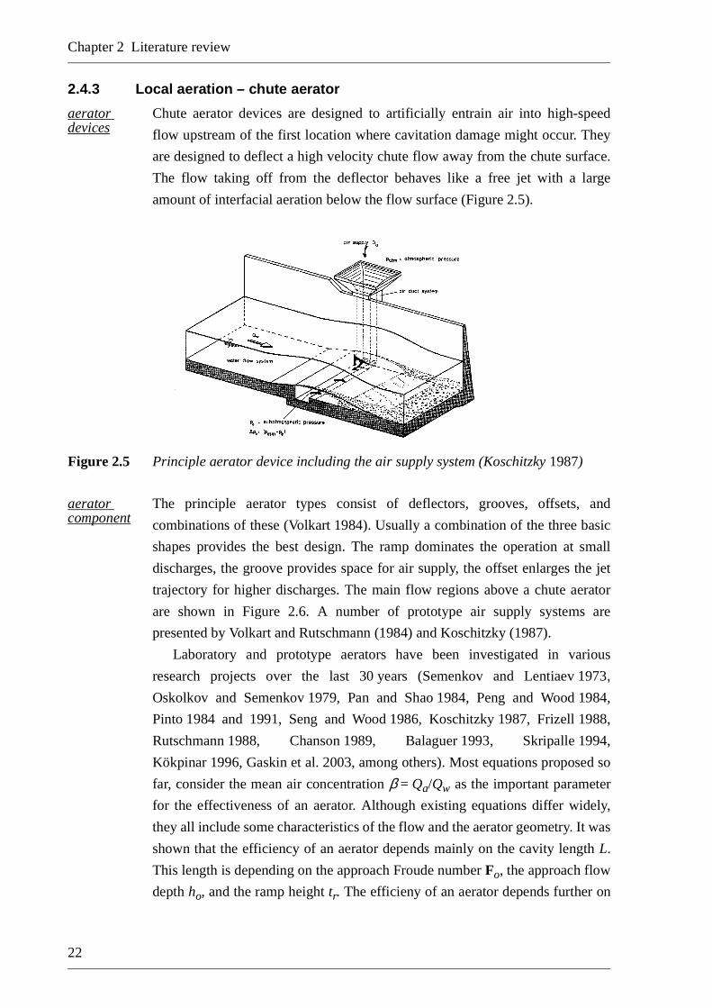
Chute aerator devices are designed to artificially entrain air into high-speed
flow upstream of the first location where cavitation damage might occur. They
are designed to deflect a high velocity chute flow away from the chute surface.
The flow taking off from the deflector behaves like a free jet with a large
amount of interfacial aeration below the flow surface (Figure 2.5).
Figure 2.5 Principle aerator device including the air supply system (Koschitzky 1987)
aerator component
The principle aerator types consist of deflectors, grooves, offsets, and
combinations of these (Volkart 1984). Usually a combination of the three basic
shapes provides the best design. The ramp dominates the operation at small
discharges, the groove provides space for air supply, the offset enlarges the jet
trajectory for higher discharges. The main flow regions above a chute aerator
are shown in Figure 2.6. A number of prototype air supply systems are
presented by Volkart and Rutschmann (1984) and Koschitzky (1987).
Laboratory and prototype aerators have been investigated in various
research projects over the last 30 years (Semenkov and Lentiaev 1973,
Oskolkov and Semenkov 1979, Pan and Shao 1984, Peng and Wood 1984,
Pinto 1984 and 1991, Seng and Wood 1986, Koschitzky 1987, Frizell 1988,
Rutschmann 1988, Chanson 1989, Balaguer 1993, Skripalle1994,
Kökpinar 1996, Gaskin et al. 2003, among others). Most equations proposed so
far, consider the mean air concentration β = Qa/Qw as the important parameter
for the effectiveness of an aerator. Although existing equations differ widely,
they all include some characteristics of the flow and the aerator geometry. It was
shown that the efficiency of an aerator depends mainly on the cavity length L.
This length is depending on the approach Froude number Fo, the approach flow
depth ho, and the ramp height tr. The efficieny of an aerator depends further on

Development of Aerated Chute Flow
23
the cavity subpressure ∆p and the turbulence number Tu. In the context of the
present project only a short summary is given, more detailed information may
be found in Kells and Smith (1991) and Skripalle (1994).
Figure 2.6 Air entrainment mechanism by an air slot including the bottom pressure po andthe bottom air concentration Cb (Volkart and Rutschmann 1984)
classical approach
Hamilton 1984, Pinto and Neidert 1983, Bruschin 1987, among others,
suggested a classical approach derived from two–dimensional aerator
investigations. Hamilton 1984 proposed
(2.17)
where qa is the specific air entrainment per meter chute width, K is a constant, u
the average approach flow velocity, and L is the jet trajectory length. He
proposed for air entrainment into the lower surface a coefficient
0.01 K 0.04 found from model and prototype measurements. Kells and
Smith (1991) proposed a relation for the air-water discharge ratio after
substituting the specific water discharge qw = uhw in equation (2.17) as
. (2.18)
qa KuL=
β KLhw------ =

Chapter 2 Literature review
24
Rutschmann (1988) presented an equation where the pressure gradient ∆p = 0
below the nappe and the atmosphere is neglected
, (2.19)
and a general equation including the approach Froude number
(2.20)
trajectory length and Froude number
where air entrainment is described as a function of the jet trajectory length,
water depth and Froude number, as deducted from model studies. Equation
(2.19) was analysed by Pfister (2002) and applied on his model investigations
with a scale of λ = 12.9. The aerator was located downstream of a spillway crest
and upstream of a stepped cascade. He proposed β = 0.006L/hw – 0.002 and
thus less air entrainment compared to Rutschmann (1988).
pressure coefficient
Koschitzky (1987) based his investigations on an approach presented by
Wood (1984) including a non-dimensional pressure coefficient ∆p/(ρwgh). He
employed a two-dimensional aerator model of variable aerator geometries,
pressure below the nappe and variable Froude numbers and obtained the
equation
(2.21)
with 0.0205 ≤ C1 ≤ 0.0253, 0.0001 ≤ C2 ≤ 1.4447, C3 ≈ 1.5 and 3.5 ≤ Fc ≤ 4.2,
where Fc is the critical Froude number for inception of air entrainment.
bottom roughness and turbu-lence
Based on Koschitzky’s equation, Balaguer (1992) included the influence of
bottom roughness and thus turbulence in the bottom region. He found that
bottom roughness has a major effect on the air entrainment below an aerator
device, which he proved using an adapted linear constant C1 in equation (2.21).
Bretschneider (1989) questioned the approaches containing a constant term C1
and the critical Froude number Fc (e.g. Koschitzky 1987, Balaguer 1992) and
initiated the dissertation of Skripalle (1994). The finding of this project was
(2.22)
β 0.0372Lhw------ 0.2660–= ∆p 0=
β 0.0493Lhw------ 0.0061Fo
2– 0.0859–=
β C1 Fo Fc–( )C3 1 C2
∆pρwgh-------------–
=
β 0.91
hw2
--------cf'
2----- δL tr L∆p 0= L–( )–[ ]≈

Development of Aerated Chute Flow
25
provided W > 170 and L/hw < 540W/R5/8 with W as the Weber number and R
as the Reynolds number. Equation (2.22) includes the ramp height tr, local
losses of the aeration device cf ’ , and the turbulent boundary layer thickness δ at
the aerator.
air detrain-ment down-stream of an aerator
Chanson (1988) studied the air entrainment and aeration devices of a
spillway model. Using the data of Peng and Wood (1984), and Seng and
Wood (1986), he concluded that air entrainment is strongly related to the jet
trajectory length and the subpressure below the nappe. Furthermore, he
mentioned that the experimental results suggest a strong de-aeration process
occurring in the impact region, but, that at this time, the measurements
instrumentation was not able to investigate local details.
air concen-tration measure-ments
All equations mentioned are based on air entrainment from below an aerator
device. Only average air concentrations have thus been investigated. Seng and
Wood (1986) and Balaguer (1993) measured air concentration profiles
downstream of an aerator, as shown in Figure 2.7, where tr is the deflector
height. At the downstream aerator end (x = 0) 100 % air prevails in the air
cavity up to z= 60 mm (Figure 2.7a) and tr/z = 0.2 (Figure 2.7b), followed by
practical 100 % water between 60 ≤ z ≤ 110 mm and 0.2 ≤ tr/z ≤ 1.25,
respectively. Close to the flow surface the air concentration varies within a short
reach from black water (C = 0) to pure air (C = 1). At L ≅ 1300 mm (Figure
2.7a) and xi/z ≅ 9 (Figure 2.7b), the lower jet nappe impinges on the chute
bottom with the bottom pressure equal to pb = 0. More downstream, the air
concentration reduces drastically in the bottom region, whereas it increases in
the middle region. Note the maximum bottom pressure pb at location xi/
z= 14.85 which was used by Rutschmann (1988) to define the length of the jet
trajectory (Figure 2.7b).
a)

Chapter 2 Literature review
26
b)
Figure 2.7 Air concentration contours downstream of an aerator fora) F = 10.7 (Seng and Wood 1986), and b) F = 8.0 (Balaguer 1993)
facit It can from this section be concluded that local aeration or aerators on chutes
have been investigated in several projects. Most of these research focused on
the amount of air entrained below the jet trajectory, depending on the aerator
geometry and hydraulic boundary conditions. The flow regime downstream of
the aeration device was investigated in two projects but not further analysed.
More research is thus needed to understand the effect of the aerator to the flow.
2.5 Air detrainment process
2.5.1 Single bubble in stagnant water
bubble rise velocity in stagnant water
The transport process of a single air bubble in water is the basis for air
detrainment on chutes. According to Falvey and Ervine (1988), it is influenced
by four main forces, namely: (1) Inertial, (2) Drag, (3) Buoyancy, and (4)
Turbulent eddy transport forces. Additionally, Rutschmann et al. (1986) found a
dependency of the non-hydrostatic pressure gradient on the bubble rise velocity,
whereas Kobus (1991) mentioned an influence of bubble clouds on the single
bubble transport process. Figure 2.8 shows the various forces acting on an air
bubble in a chute flow. The transport process of a single air bubble in stagnant
water is reviewed in this section.
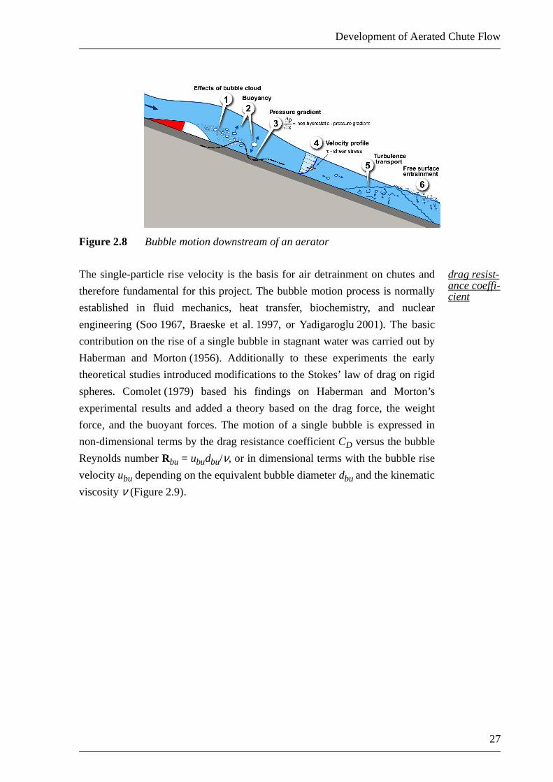
Development of Aerated Chute Flow
27
Figure 2.8 Bubble motion downstream of an aerator
drag resist-ance coeffi-cient
The single-particle rise velocity is the basis for air detrainment on chutes and
therefore fundamental for this project. The bubble motion process is normally
established in fluid mechanics, heat transfer, biochemistry, and nuclear
engineering (Soo 1967, Braeske et al. 1997, or Yadigaroglu 2001). The basic
contribution on the rise of a single bubble in stagnant water was carried out by
Haberman and Morton (1956). Additionally to these experiments the early
theoretical studies introduced modifications to the Stokes’ law of drag on rigid
spheres. Comolet (1979) based his findings on Haberman and Morton’s
experimental results and added a theory based on the drag force, the weight
force, and the buoyant forces. The motion of a single bubble is expressed in
non-dimensional terms by the drag resistance coefficient CD versus the bubble
Reynolds number Rbu = ubudbu/ν, or in dimensional terms with the bubble rise
velocity ubu depending on the equivalent bubble diameter dbu and the kinematic
viscosity ν (Figure 2.9).

Chapter 2 Literature review
28
Figure 2.9 Bubble rise velocity in still water as a function of bubble size (Haberman andMorton 1956)
equations describing the experi-mental data
The equations for the dimensional rise velocity based on Haberman and
Morton’s experimental data are plotted in Figure 2.9. Starting from a small rigid
sphere bubble, surface tension determines the transport process. The bubble rise
velocity for small air bubbles dbu < 0.068 mm can be written according to
Stokes as (Falvey 1980)
. (2.23)
For slightly larger air bubbles, say 0.068 < dbu < 0.80 mm, the bubble rise
velocity follows
. (2.24)
changing of bubble shape
With increasing bubble size, the bubble shape changes from spherical to oblate
spheroid with the bubbles rising along an irregular or spiral trajectory
(Kobus 1991).
(2.25)
(2.24)
(2.23)
ubu29---
dbu2
g
νw----------- 1
ρa
ρw------–
=
ubu118------
dbu2
g
νw----------- 1
ρa
ρw------–
=

Development of Aerated Chute Flow
29
Comolet (1979) observed that both surface tension and buoyant forces are
important, and suggested therefore
(2.25)
large bubbles
for bubbles 0.8 < dbu < 10 mm. For bubbles exceeding dbu > 10 mm surface
tension effects can be neglected and the rise velocity follows simply
(Falvey 1980)
. (2.26)
2.5.2 Single bubble in turbulent flow
Turbulence
shear stress fractures the bubbles
The following points have been mentioned to describe the bubble rise velocity
in turbulent flows. Flow turbulence introduces shear which tends to fracture a
bubble into smaller bubbles. Falvey (1980) proposed a procedure to estimate
the critical bubble size dbu(95) from the loss of energy as shown by
Hinze (1975). He therefore included an equation suggested by Rouse (1970) for
the loss of energy by the slope of energy SE to calculate the critical bubble size
as
(2.27)
with dbu(95) as the bubble diameter for which 95 % of the air is contained in
bubbles of this diameter or smaller.
The effect of turbulence reduces the terminal bubble rise velocity. If ubu is the
terminal rise velocity of bubbles in still water, then ubut is the terminal rise
velocity in turbulent flow. Their relation can be expressed as ubut = a ubu where
a is an empirically determined variable according to Figure 2.10. Note that the
variable a is always positive consequently this relation includes only rising
bubbles, the entraining part due to the turbulence downstream of the point of
inception is not considered here.
ubu 0.52gdbu 2.14σt
ρwdbu--------------+=
ubu gdbu=
dbu 95( ) 0.725σt
ρw------
3 1
gSEu------------
215---
=

Chapter 2 Literature review
30
Figure 2.10 Terminal rise velocity of bubbles in turbulent flow (Falvey 1980)
bubble break-up
Chanson and Toombes (2002) supported Falvey’s idea with new model tests.
They concluded that the presence of finer bubbles was a result of bubble
break-up by turbulent shear.
Bubble clouds
bubble clouds
A bubble cloud in stagnant water moves with a considerably larger mean
velocity than a single bubble due to the fact that the bubble swarm induces an
upward water flow. If the water has a horizontal velocity component, this effect
is counteracted in the same order of magnitude by the fact that the bubbles are
displaced laterally along their path and hence the induced vertical water flow is
less pronounced (Kobus 1991).
loss of kinetic energy
Volkart (1985) explained the reduced rise velocity in his laboratory
investigations by the fact that a large number of bubbles result in mutual contact
and interference. The result will be collisions, deformations, collapse of bubbles
and coalescence and thus a loss of kinetic energy and higher drag of air bubbles.
Non-hydrostatic conditions
non-hydro-static pres-sure gradient
Rutschmann et al. (1986) found that the bubble rise velocity in the impact zone
of jets onto the chute bottom is effected by a non-hydrostatic pressure gradient.
They further mentioned an equation showing strong dependence on the vertical
pressure gradient dp/dz on the bubble’s rise velocity, because the balance
between the upward turbulent diffusion and the downward pressure gradient

Development of Aerated Chute Flow
31
affects bubble motion. Their equation proposed was dimensional inconsistant
but gives an idea of the influence of the non-hydrostatic pressure gradient on the
bubble rise velocity.
bubbles are captured in the flow for negative pressure gradients
Wood (1988) mentioned a similar equation to predict the bubble rise
velocity in non-hydrostatic pressure conditions. He linked results of
Rutschmann et al. (1986) and Chanson (1988) and described that in the impact
zone the pressure reaches a maximum several times greater than normal
hydrostatic pressure. This much larger pressure leads to steep pressure gradients
and large quantities of air detrained from along the flow in the impact region.
Chanson (1997) found that the non-hydrostatic pressure gradient is also
jointly responsible for the bubble rise velocity. He mentioned a simplified
method to approximate the bubble rise velocity as
(2.28)
where ubu is estimated from the bubble rise velocity in stagnant water using
equation (2.23)
The bubble transport direction depends on the algebraic sign of the pressure
gradient, thus bubbles rise towards the free surface for dp/dz > 0, and bubbles
are captured in the flow if dp/dz < 0. Figure 2.8 shows air bubbles downstream
of an aerator subjected of the above outlined influences.
2.6 Air detrainment from chute flow
2.6.1 Detrainment zones
detrain-ment process
The air bubble motion is affected by a number of complicated and poorly
investigated processes. Therefore, direct experimental investigation of the
detrainment process was used rather than investigations on single bubbles. For
flows discussed in this project unlimited air escape and supply to and from the
atmosphere was considered, as suggested by Kobus (1991). Before approaching
the overall air detrainment process, the chute flow has to be divided into zones,
as shown in Figure 2.6. Furthermore, combining the de-aeration zone
downstream of the aerator with the development of self-aerated flow as shown
in Figure 2.11, the following classification may be proposed: (1) Approach
zone, (2) Transition zone, (3) Aeration zone, (4.1) Detrainment zone in
combination with developing partially aerated flow, (4.2) Detrainment zone in
combination with developing, fully aerated flow, and (5) Fully developed,
aerated equilibrium flow (Falvey 1980).
ubut2
ubu1
ρwg---------
dpdz------=

Chapter 2 Literature review
32
Figure 2.11 Air entrainment flow regimes in open channel flow (Falvey 1980)
If the transport capacity of the flow is low, the entrained air escapes rather
quickly, whereas the air is captured in the flow with large transport capacity
(Wood 1985). Furthermore, the air detrainment process is directly linked to the
free-surface entrainment since the air concentration reaches an equilibrium state
at a point where the air entrained by turbulence is equal to the air detrained (see
2.4.2).
2.6.2 Aerator spacing
location of aerators
The first aerator is located upstream of the first point of cavitation inception
(see 2.2.2). The distance to the second aerator depends on: (1) The air
detrainment rate downstream of the first aerator, and (2) The natural aeration
from the free surface. Normally, free surface aeration does not reach the chute
bottom in regions where the first aerator should be placed (Volkart and

Development of Aerated Chute Flow
33
Rutschmann 1984), whereas Chanson (1989) affirmed that no further aerator is
required for spillway slopes in excess of α > 20 °. Figure 2.12 shows the
principle alignment of aerators on chutes including the streamwise
developments of the critical cavitation number, the air duct aeration, the air
detrainment and the free surface aeration. Recommended design guidelines
published in the literature are presented below. It has to be emphasised that
aerators are not always placed according to current design guidelines but are
often located at gates or transitions between straight and negative curvatures to
simplify the design or to accommodate other features of the chute. Up to now
there has been a trend towards designing more aerators on prototypes than
necessary to stay on the safe side.
Figure 2.12 Alignment of aerators and two-phase flow hydraulics (Koschitzky 1987)
To predict the reduction of air concentration as a function of distance, the
following approaches have been proposed.
Linear air detrainment on chutes
air detrain-ment found on Russian prototypes
First rough approximations for the air detrainment process downstream of a
chute aerator were derived from investigations carried out in the 1970’s on
Russian’s high head dams (Gal’perin et al. 1979). Oskolov and
Semenkov (1979) noted a maximum average air concentration of 45 % because

Chapter 2 Literature review
34
a higher concentration would result in significant spray. Based on this
assumption, Semenkov and Lantyaev (1973) proposed for the reduction of air
concentration in straight sections
∆C = 0.40 – 0.80 %/m. (2.29)
higher loss rate in the bottom layer
They also noted a loss rate in a 1 cm thick bottom layer 1.5 to 2.0 times higher
than the average loss rate. Prusza (1983) mentioned the linear air reduction rate
∆C per meter, depending on the cross-sectional shape of the chute
∆C = 0.15 – 0.20 %/m for straight sections,
∆C = 0.50 – 0.60 %/m for concave sections (buckets),
∆C = 0.15 – 0.20 %/m for convex sections. (2.30)
Minor (2000) derived a smaller reduction of detrained air from video records of
the Restitucion spillway in Peru over the entire length as
∆C = 0.10 – 0.15 %/m. (2.31)
aerator distance depending on the bottom air concentra-tion
Vernet et al. (1988) measured the air concentration in the centreline of the
operating Alicura dam spillway. Four aerators are distributed over the b = 39 m
wide, So = 35 % steep, straight spillway with a streamwise aerator spacing of
63 m. They mentioned that the bottom air detrainment Cb,det between aerators 1
and 2 was larger than between aerators 3 and 4. However, even if some
discrepancies in the measuring system calibration are admitted, the following
numbers for bottom air detrainment per meter chute length were proposed
∆Cb,det = 0.45 %/m bottom air detrainment, aerators 1 and 2,
∆Cb,det = 0.26 %/m bottom air detrainment over the chute. (2.32)
Distance between aerators
On the basis of model tests, Lesleighter and Chang (1981) proposed for the
requried aerator spacing the length
∆L = 40 m. (2.33)
direct aerator spacing method
Pinto et al. (1982) summarised experience of several prototype spillways
including the aerator spacing. They found that some of the designed aerators
had to be eliminated because of too much air entrained, such as for Bratsk,
Nurek, Foz do Areia, Emborcacão, and Guri spillways. They concluded that a
well designed aerator should protect a chute lenght of about
∆x = 50 – 100 m. (2.34)

Development of Aerated Chute Flow
35
With equation (2.29), a maximum air concentration of 45 %, 8 % minimum air
concentration for damage protection, and a decay rate of 0.4 – 0.8 % per meter
chute length, the required spacing would result in (Kells and Smith 1991)
∆x = 46.3 – 92.5 m maximum spacing, and
∆x = 23.1 – 46.3 m minimum spacing. (2.35)
Aerator spacing depending on flow properties
flow prop-erties – responsi-ble for aerator spacing
Vischer et al. (1982) presented an approach for the distance ∆x required
between two aerator slots depending directly on the average flow velocity um.
Kells and Smith (1991) derived from data presented by Volkart and
Chervet (1983) the aerator spacing relationship
∆x = 1.1 um. (2.36)
Equation (2.36) was derived from a dimensionally inconsistent figure. Nokes
suggested in a discussion with Wood (1984) a cavitation free chute length of
∆xf = 12 hw, (2.37)
and markedly reduced one
∆xr = 50 hw, (2.38)
depending on the flow depth hw.
hydraulic conditions influence bottom air concentra-tion
Volkart and Rutschmann (1984) presented air bottom concentration
measurements downstream of a model aerator taken 10 cm above the chute
bottom (Figure 2.13). They mentioned that the air distribution depends mainly
on the distance to the side wall and the local Froude number. However, no
design guideline was derived from those measurements. Whereas
Volkart (1985) compared bubble rise velocities in turbulent flow ubut with the
measured value in still water ubu which can be deducted from Figure 2.9, and
found that the bubbles actually rise 10 times slower under turbulent conditions
. (2.39)
He therefore concluded that flow bubbles rise slower in turbulent flow than in
still water.
ubut
ubu
10-------=

Chapter 2 Literature review
36
Figure 2.13 Air concentration profiles along chute bottom (Volkart and Rutschmann 1984)
Self aeration and equilibrium flow conditions
exponen-tial aera-tor distance including the amount of air
According to Falvey (1990), May (1987) suggested an exponential approach to
describe the air detrainment process instead of a linear. He included the average
air concentration Co upstream of the aerator and the point of inception xi
downstream of the aerator. Because downstream flow of an aerator is influenced
by Co and xi, the air detrainment process was approximated with
(2.40)
with xa as the streamwise distance measured from the aerator end.
Falvey (1990) proposed to include the free surface-aeration of the flow (see
2.4.2) and therefore generalized equation (2.40) to
(2.41)
where the uniform air concentration Cu may be calculated using equation (2.13)
or (2.14).
equilibri-um condi-tions influence the aerator location
The air concentration downstream of an aerator has been analysed by
Chanson (1989) by comparing model and prototype investigations on the
Aviemore and Clyde dam spillways. He mentioned that the air concentration
distribution in the downstream flow region tends to the equilibrium distribution.
Chanson therefore concluded with respect to Straub and Anderson’s (1958)
data, that an equilibrium average air concentration Cu > 30 % would be
sufficient to obtain 5 % bottom air concentration for spillway protection and
thus proposed only one aerator on spillways exceeding α > 20 ° bottom slope.
Although that he proposed two equations for uniform air concentration Cu and
specified the bubble rise velocity with ubu = 0.16 m/s for hydraulic models, and
ubu = 0.40 m/s for prototype chutes, both Cu and ubu seem rather uncertain.
C x( ) Coe0.0– 17 xa xi–( )
=
C x( ) Co Cu–( )e0.0– 17 xa xi–( )
=

Development of Aerated Chute Flow
37
Vischer and Hager (1998) simplified an approach for the local change of air
concentration by Chanson (1989) including equilibrium air concentration and
the bubble rise velocity to
. (2.42)
2.7 Focus of the present project
2.7.1 Summary of previous studies
from cavi-tation damage to aerator spacing
This chapter is a literature review based on cavitation formation due to low
pressures and high velocities on chutes and demonstrated that aeration seems to
be an adequate and technically feasible method to prevent cavitation damage on
dam spillways. Furthermore, two typical aeration methods were analysed,
namely: (1) Free surface aeration and (2) Aerator devices. The boundary
conditions for free surface aeration and the efficiency of aerators were cited.
The review started with the single bubble rise velocity in still water and was
linked to air detrainment in supercritical, high turbulent flow conditions. The
effects of non-hydrostatic pressure gradient, bubble clouds and turbulence were
included.
reduced bubble rise velocity due to turbulence
Air detrainment in chute flows is much slower than air bubbles of the same
size rise in stagnant water. This may be explained by two approaches: (1) The
air bubbles are fractured into smaller size due to shear stress, and (2) The
turbulence captures the air bubbles in the flow. Theory (2) has dominated up to
present times and is considered responsible for the air detrainment process
without further evidence. Difficulties to measure turbulence in two-phase flows
can be traced back to the lack of appropriate measuring instrumentation.
developing region
The fact that one aerator is sufficient in the fully developed flow region was
often mentioned, but there has no attempt been made for solving the problem in
the developing region. The current design criteria for aerator spacing were
summarised, starting from a simple linear approach to more complex including
flow velocity, flow depth, spillway slope, surface tension and free surface
aeration. It was stated that all theories are currently based on prototype
observations or limited laboratory tests. The current design criteria are
conservative and entail too much air in the flow, which was proven on prototype
spillways where aerator devices were closed due to over-aeration and
super-saturation of the flow.
dqa
dx-------- C Cu–( )ubu αcos=

Chapter 2 Literature review
38
2.7.2 Research gaps
unspeci-fied quanti-ties of air for protec-tion needed
1. There is little knowledge of the physical effect of air on cavitation
damage. The numbers of 5 % to 8 % air required, established for
different conditions, to protect a concrete surface are still used today
after more than 50 years. Further research is needed to confirm these
numbers and to expand the theory to find the amount of air needed for
appropriate cavitation protection in chute boundary region.
new model data need-ed for the air detrain-ment proc-ess
2. For aerator spacing simple approaches are still common due to the lack
of fundamental knowledge. The development of air concentration in
pre-aerated chute flow has not been undergone systematical attention.
The free-surface aeration is an important part which was often
neglected so far. It has been emphasized that more laboratory data in
the downstream area of an aerator are needed to understand the
features of detrainment and entrainment in such hydraulic structures.
2.7.3 Focus of the present research study
Point (1) mentioned above is important for cavitation protection and must be
investigated in future. Point (2) is also an urgent topic to investigate because
even fewer knowledge is available for it. The present study focuses on the
second point therefore, to explain the essentials of the streamwise behaviour of
two-phase flow downstream of an aerator.

Development of Aerated Chute Flow
39
CHAPTER 3 PHYSICAL MODEL
3.1 Introduction
For a complex hydraulic problem experimental investigations are still the most convenient
solution. The 14 m long chute model used for the two-phase investigations had a variable
bottom slope, a variable inflow depth and a frequency-regulated pump. The automatically
driven measuring system was based on a fiber-optical probe manufactured by RBI, Grenoble.
The large data sets were collected and analysed automatically with a graphical user interface
based on Matlab. Preliminary investigations were conducted to verify the accuracy of the
measurements. Finally a dimensional analysis was carried out to determine the relevant scales
of the hydraulic parameters.
3.2 Experimental set-up
basic channel set-up
The experiments were conducted in a prismatic rectangular channel, located in
the Laboratory of Hydraulics, Hydrology and Glaciology (VAW), ETH Zurich.
The model was primarily built by Lauber (1997) to investigate dam break
waves. All devices are described in detail in his thesis; therefore, only relevant
and modified components are presented in this chapter. All model elements
involving the measuring technique applied are shown in Figure 3.1 and Table
3.1.
model details
The hydraulic model was built in a chute, of width b = 0.50 m, length
l = 14 m and with a variable bottom slope 0 % So 50 %. The channel floor
was PVC made with an assumed equivalent sand roughness ks = 0.01 mm. The
sand roughness obtained from measurements under uniform flow conditions
was calculated to a roughness height of ks = 0.00023 mm, using the
Darcy-Weisbach equation (see 3.4.3). To investigate the roughness influence on
the air-detrainment and air-entrainment processes, an artificial roughness was
installed on the channel bed. The material used had a thickness of ks = 2.50 mm.
Measurements with the roughened surface were carried out early in the present
project, and are mentioned in the according chapters.

Chapter 3 Physical model
40
data collection
All quantities, namely: (1) Water discharge Qw, (2) Air discharge Qa, (3)
Positioning in the x- and z directions, and (4) automised data collection, were
controlled by a LabView based program designed at VAW. Automatic data
acquisition, i.e. air concentration profiles, velocity field and characteristic
mixture flow depth h90, was performed by a program based on Matlab.
Figure 3.1 Physical model including the measuring system
Table 3.1 Instrumentation used for the two-phase flow investigations
No. instrumentation quantity unit range accuracy controlunit
input / output
frequency controlled pump
water discharge
Qw
m3/s 0–0.250 ± 2 % PC 4–20 mA
gate valve manual
swing type check valve
automatic
inductive flow meter (IDM)
water discharge
Qw
m3/s 0–0.30 ± 1 % PC 4–20 mA
pressure valveair pressure
pabar 0–16 manual
1
2
3
4
5

Development of Aerated Chute Flow
41
3.2.1 Water discharge
water flowWater discharge Qw up to 250 l/s was provided with a frequency-regulated
pump KSB ETA-R-250-300 , and controlled by a frequency converter
produced by H.P. Rey AG. The water discharge was measured to ± 1.0 % by an
Inductive Discharge Meter (IDM) RHEOMETRON AG , and conducted
through a jetbox built at VAW, as described by Schwalt and Hager (1992).
The jetbox allowed independent variation of the inflow depth ho and thus the
inflow Froude number
. (3.1)
air flow meterair discharge
Qam3/h 0–300 ± 5 % PC 4–20 mA
air pressure gaugeair pressure
pabar 0–16 manual
jetboxinflow depth
hom 0–0.12 ± 0.1 mm manual
thermoelectricanemometer
air velocityua
m/s 0.15–5.0 ± 1.5 % PC 4–20 mA
chute
aerator ramp tr mm 15
remote controlled travelling system
positioningx / z
m0–14.00–0.50
± 1 mm PC
fiber-optical probe
air concentra-tion C
[–] 0–100± 5 %
(see 3.4)PC
digital signal
fiber-optical probe
mixture flow velocity um
m/s 0–15± 5 %
(see 3.4)PC
digital signal
fiber-optical probe
bubble size dbu
mm
back flow to the closed circuit
lab computer and analogue/digital
converter
No. instrumentation quantity unit range accuracy controlunit
input / output
6
7
8
9
10
11
12
13a
13a
13a
14a
15a
1
4
8
Fo
Qw Qa+
b gho3
--------------------=

Chapter 3 Physical model
42
Energy was dissipated in a plunge pool at the end of the chute before closing the
circuit back to the pump sump below the channel .
3.2.2 Aeration device
air supply Three different set-ups for air addition to the water flow were employed,
namely: (1) Pre-aerated discharge supply to obtain a well-defined upstream
cross-section of the air-water mixture, (2) Chute aerator as used on prototypes,
and (3) Free-surface aeration where air was entrained from the turbulent surface
boundary layer with no additional forced aeration. For pre-aerated air discharge
Qa was added to the supply pipe (Figure 3.1 and Figure 3.2 a), whereas the
air was entrained into the aerator for chute aerator flow (Figure 3.2 b and Figure
3.3). The air added was supplied from a compressed air system, the pressure
was adjusted to ± 2 % by an air pressure valve (Figure 3.1 and Figure 3.2 a).
The air discharge Qa was limited to 55 l/s, measured by an air flow meter
equipped with an electronic transmitter WISAG Typ 250 (Figure 3.1 and
Figure 3.2 a).
a) b)
Figure 3.2 a) Air discharge meter, pressure valve, and Inductive Discharge Meter (IDM),b) Air supply system (air duct) for atmospheric pressure and thermoelectricanemometer
air distribu-tion below the aerator
The chute aerator was a tr = 15 mm high and lr = 150 mm long step made of
PVC in the early stage of the project; aluminium was used for better stability
later (Figure 3.3). The air was supplied through an air duct on the left side wall
into the deflector (Figure 3.1 and Figure 3.2 b). The air velocity in the duct
14
7
5
6
9

Development of Aerated Chute Flow
43
was measured with a thermoelectric anemometer Schiltknecht ThermoAir64 dir
and multiplied with a distribution coefficient to obtain the cross-sectional air
discharge Qa with a accuray of ± 5 % (Pfister 2002). The distribution
coefficient was based on the logarithmic velocity distribution for fully turbulent
flow. The thermoelectric anemometer and the air flow meter were connected to
the PC, which enabled permanent monitoring of the air and water discharges.
An air supply system causes internal frictional head losses, as discussed by
Haerter (1961), Koschitzky (1988), and Rutschmann and Volkart (1988). There
is a lower pressure at the inflow aerator side due to the higher velocity; thus the
air distribution rate is not uniform over the aerator width. Losses were
compensated by external substitution from the compressed air system and the
distribution was improved by air contribution through various holes in flow
direction. The holes were arranged such that the distribution was symmetric and
almost two-dimensional (Figure 3.3).
Figure 3.3 Model chute aerator
3.2.3 Automated data collection
remote controlled positioning system
The remote controlled positioning system Phoenix Mecano AG mainly carried
and positioned the fiber-optical measuring probe (Figure 3.4). The positioning
was controlled by the PC and enabled measurements to be taken for any
coordinates in the x- and z-directions along the channel axis. The accuracy of
the longitudinal position x and the vertical position z perpendicular to the chute
bottom was ± 1 mm. Normally 19 streamwise increasing cross sections were
taken along the channel with 35 perpendicular measurements. Thus, 665
readings of local air concentration, local velocity, and bubble size are the frame
of data for later evaluation.
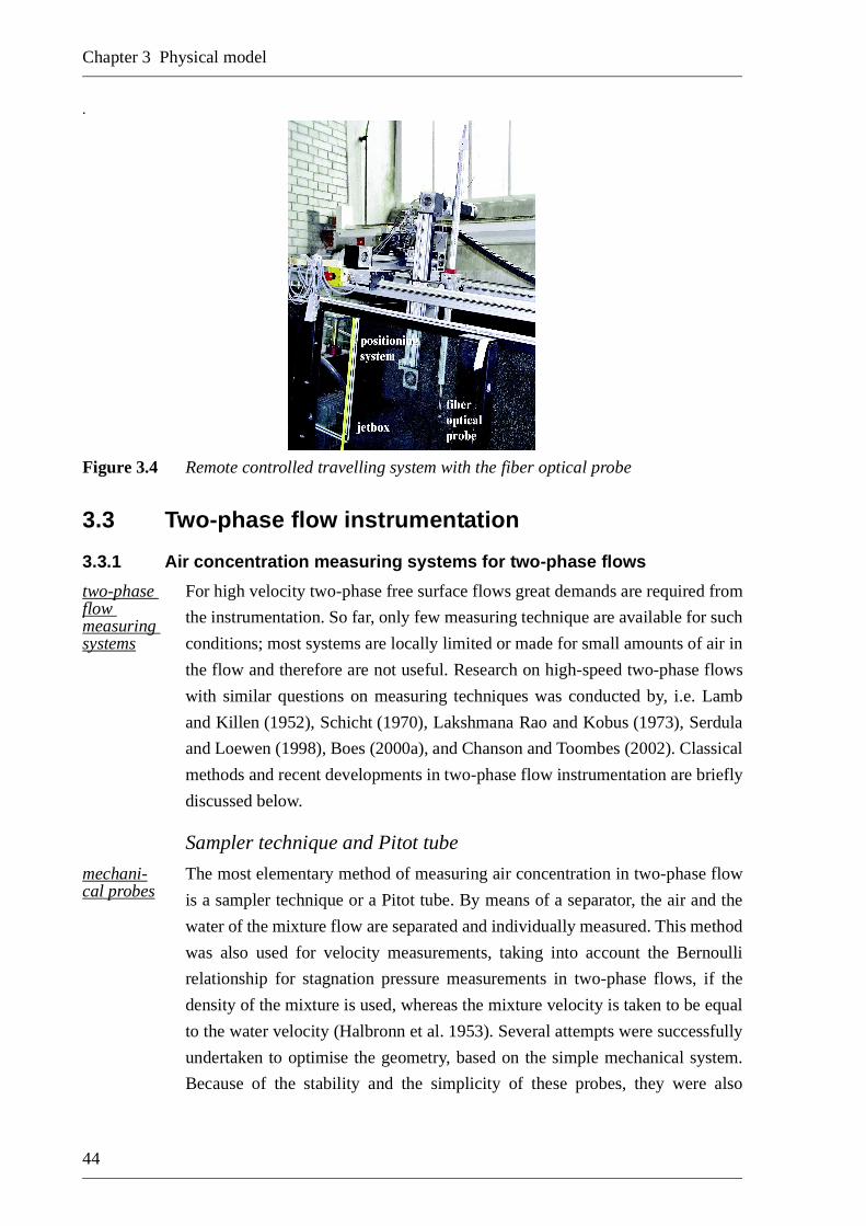
Chapter 3 Physical model
44
Figure 3.4 Remote controlled travelling system with the fiber optical probe
3.3 Two-phase flow instrumentation
3.3.1 Air concentration measuring systems for two-phase flows
two-phase flow measuring systems
For high velocity two-phase free surface flows great demands are required from
the instrumentation. So far, only few measuring technique are available for such
conditions; most systems are locally limited or made for small amounts of air in
the flow and therefore are not useful. Research on high-speed two-phase flows
with similar questions on measuring techniques was conducted by, i.e. Lamb
and Killen (1952), Schicht (1970), Lakshmana Rao and Kobus (1973), Serdula
and Loewen (1998), Boes (2000a), and Chanson and Toombes (2002). Classical
methods and recent developments in two-phase flow instrumentation are briefly
discussed below.
Sampler technique and Pitot tube
mechani-cal probes
The most elementary method of measuring air concentration in two-phase flow
is a sampler technique or a Pitot tube. By means of a separator, the air and the
water of the mixture flow are separated and individually measured. This method
was also used for velocity measurements, taking into account the Bernoulli
relationship for stagnation pressure measurements in two-phase flows, if the
density of the mixture is used, whereas the mixture velocity is taken to be equal
to the water velocity (Halbronn et al. 1953). Several attempts were successfully
undertaken to optimise the geometry, based on the simple mechanical system.
Because of the stability and the simplicity of these probes, they were also

Development of Aerated Chute Flow
45
employed on prototype spillways, i.e. Hall (1943), Keller (1972), and Drewes
and Aksoy (1992). Disadvantages of those probes are the examination time, the
length of the shaft for higher velocities, the inaccuracy for high void fractions
(C > 80 %) and manual reading.
PIV – optical instrumentation
PIVThe most convenient optical method is the Partial Image Velocimetry (PIV), a
technique which uses multiple images of flow tracing particles (air bubbles in
water) in a light sheet to measure the two in-plane velocity components in an
area of interest. The optical methods are often used for tracer concentration in
chemical engineering and various applications in hydraulic modelling. This
technique enables the velocity in-plane direction to be measured as well as the
turbulence and the air concentration. It is, however, difficult or even impossible
to see optically into a highly loaded air-water mixture flow as for the present
application, thus only the wall region could be investigated for flow conditions
occurring on chutes and spillway models. Another disadvantage is that PIV is
usually limited to small areas of investigation. It is not practical to investigate a
long channel by PIV, therefore.
LDA / PDA technique
optical instrumen-tation
The plane Laser-Doppler Anemometer (LVA) measures two simultaneous
components of velocity and turbulence intensity. It is based on two independent
laser signals which define a control volume. A flowing particle (air bubble,
tracer particle etc.) in the control volume refracts, breaks and disperses the light
such that the receiver identifies the three-dimensional velocity through the
phase shift (Eigenberger 1997). Azzopardi (1999) found that measurements
made with the same equipment on single-phase gas flow showed profiles of
mean velocity and turbulence intensity similar to two-phase data. According to
Braeske et al. (1997) the Phase-Doppler Anemometer (PDA), a further
development of LDA, enables two particles with different shifting mechanisms
to be distinguished and is thus a well established non-intrusive technique for
two-phase flow with small void fractions.
X-Ray method
X-rayCommon optical methods fail, as mentioned, in bubble flows that have large
void fractions because of the different refraction indices of the liquid and
gaseous phase. X-rays penetrate a gas/liquid flow in straight lines, thus enabling
measurements of three-dimensional velocity (Seeger et al. 2001). The X-ray
method is non-intrusive but enables recording of only axial mean air

Chapter 3 Physical model
46
concentration and is thus influenced by the wall boundary layer. Additionally,
handling X-rays has a high danger potential and needs a costly safety
precaution.
ADV – Acoustic Doppler Velocimeter
acoustic systems
The Acoustic Doppler Velocimeter (ADV) has one transmitter and three
receivers. The receivers are aligned to intersect with the transmit beam at a
small sampling volume. The leading edge of the sampling volume can be placed
in flow direction such that the controlled volume is not influenced by the probe.
The ADV technique is normally not made for two-phase flows. Nevertheless,
Liu et al. (2002) mentioned that the relative error for the investigated ADV
system is a linear function of air concentration for situations with average
bubble size of about 2.5 ~ 4 mm and air concentration of up to 2.2 %. It is,
however, not useful for higher air concentrations as in the present project.
Hot film technique
hot film measuring system
The hot-film technique for measurements in air-water flows enables the
achievement of the local air concentration, the mean flow velocity and the
turbulence intensity. Its principle is based on the period of contact between one
phase and the probe being converted into electrical signals. Since the hot-film
probes are not free of inertial effects and because they have a finite time
constant, this instrumentation is no more popular in hydraulic engineering
(Lakshmana Rao and Kobus 1973).
Conductivity probes
conductiv-ity probes
An often used two-phase flow measuring system in hydraulic engineering are
conductivity probes of various designs, with one or two tips. The method was
introduced in hydraulic engineering by Lamb and Killen (1952). It is designed
to obtain air concentration measurements, which involves the determination of
the electrical resistance of the filament of fluid mixture bounded by two small
electrodes. The resistance of water is one thousand times lower than the
resistance of air bubbles, therefore each air bubble in the flow, impinging the tip
instantly increases the resistance across the probe and thus the voltage
difference across the probe will be lowered. Lamb and Killen (1952) used their
instrumentation to measure the local values of air concentration and velocity in
small increments of cross-sectional areas of the flows in the experimental
flume. Based on this conductivity system, various improvements were achieved

Development of Aerated Chute Flow
47
in the last 50 years by Lakshmana Rao et al. (1970), Cain (1978),
Volkart (1978), Bachmeier (1988), Matos and Frizell (1997), and Chanson and
Toombes (2002), among others.
double tip probes
The instrumentation is also built as a combined probe to measure both
stagnation pressure using a Pitot tube and air concentration, to improve the
accuracy of velocity predictions. Several researchers used double-tip
conductivity probes to measure air-water velocities based on a cross-correlation
technique between two identical tips aligned in the direction of the flow.
Chanson (1997) concluded that conductivity probes provide simple means for
air content and mean velocity measurements for high-velocity air-water
free-surface flows. The accuracy is reasonable, typically ∆C/C < 2 % and ∆u/
u ≈ 5 to 10 %. The operating range of conductivity probes is large for air
contents between 3 to 95 % and average velocities from 0.2 to 40 m/s.
Fiber optical probe
fiber optical probes
Fiber optical probes are sensitive to the change in the refractive index of the
surrounding medium. Emitted light hitting the sensitive tip surface is refracted
when liquid surrounds the tip, and reflected when gas is present. Consequently,
bubbles and droplets can be detected at a given point in the flow. Among other
information, the optical probe permits measurements of local void fraction and
arrival frequency of bubbles and droplets. Using two sensors and
cross-correlation, information is obtained on mixture velocity (RBI 2000). With
its double-tip principle, velocity measurements can be achieved similarly to the
conductivity probes system.
perform-ance and accuracy
Various investigations were performed concerning the accuracy of
fiber-optical probes. Cartellier and Achard (1991) reviewed the performance of
various techniques for measuring void fraction. They found that fiber optical
probes, Photonetics, Inc, produce a relative error ranging in the worse from –
56 % to +11 % depending on the void fraction. They therefore stated that the
use of fiber-optic probes to measure very small void fractions is not
recommended because of the large errors that may be anticipated. Serdula and
Loewen (1998) disagreed after placing the same probe perpendicular to the
flow, and concluded that the technique can be used to make reasonably accurate
measurements of the void fraction even in a dispersed regime (Liu et al. 2002).
Boes (2000a) stated that after several pre-measurements with his fiber optical
probe RBI, Grenoble, the system measures void fraction and flow velocity with
an error of smaller than ± 5 %. The main disadvantage of this instrumentation is

Chapter 3 Physical model
48
the lack of supplementary flow information, i.e., velocity fluctuation and
turbulence information; others are the probe intrusiveness, the highly fragile
probe tips and the one dimensionality of flow information.
3.3.2 Probe used in the present project
fiber optical probe RBI-Grenoble
A fiber-optical probe manufactured by RBI, Grenoble, introduced by Boes and
Hager (1998) and Boes(2000a) was used in this project to measure the
following quantities: (1) Local air concentration C, (2) Mixture flow velocity
um, and (3) Bubble diameter dbu, besides various other statistical parameters.
The basic principle of the fiber-optical instrumentation is described by
Boes (2000a) and the RBI (2000) users Guide for VIN 2.0; therefore, only the
significant software modifications implemented for this project are described
here. Figure 3.5 shows a) the fiber-optical probe and b) the opto-electronic
amplification module, which transforms the analog signal obtained from the
probe into a digital Transistor-Transistor-Logic (TTL) signal which is stored on
the PC’s RAM memory. The software for the acquisition system was adapted to
the remote controlled positioning mechanism. The novel software enabled data
collection and data acquisition to handle the large data sets. The measurement
points were taken depending on the flow characteristics, e.g. flow depth, aerator
flow, pre-aeration or free surface aeration. The number of measurements were
adjusted to the air concentration gradients dC/dx and dC/dz with a streamwise
increasing spacing.
RBI – data output and processing
software altering for VIN 2.0
Figure 3.6a shows a typical data output file from the new software based on
VIN 2.0. It may be observed that the output contains more information than
mentioned above. Beside others, the main improvements to the VIN 1.0
software used by Boes(2000a) are the new software for detection of 200.000
instead of 4.000 signals (air bubbles) and the reduced computing time to handle
the large data sets. Therefore, even in regions with a high bubble frequency the
time criterion (typically 20 seconds) intercepted the measurement and not the
number of bubbles. A complete set of data was thus obtained for all
measurements.

Development of Aerated Chute Flow
49
a) b)
Figure 3.5 a) fiber-optical probe in air water mixture,b) opto-electronic amplification module and oscilloscope for thresholdadjustment
turbulenceVarious attempts were made to implement turbulence intensity to the RBI
instrumentation. So far it is not possible to follow the turbulent fluctuations. It
was tried to implement the Reynolds turbulence term, by substituting the
instantaneous velocity with the average mixture flow velocity um plus a
fluctuation term va’ . For the fluctuation term an instantaneous bubble velocity
va’ was separated from the mean mixture velocity, assuming that the bubble size
is constant, thus, u = um+ va’ . The attempt failed because of the temporally
changing bubble size. The turbulent boundary layer was finally calculated by
standard equations (e.g. Bormann 1968, Schlichting and Gersten 1996).
data processing
The data processing was executed from a Matlab-based Graphical User
Interface (GUI) (Figure 3.6b). Matlab opens the RBI data, exposes the data of
interest and compiles matrices for the two-phase flow field. All graphical plots,
evaluations and data fittings were performed from this interface.
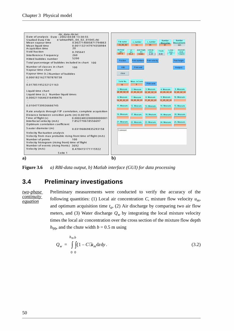
Chapter 3 Physical model
50
a) b)
Figure 3.6 a) RBI-data output, b) Matlab interface (GUI) for data processing
3.4 Preliminary investigations
two-phase continuity equation
Preliminary measurements were conducted to verify the accuracy of the
following quantities: (1) Local air concentration C, mixture flow velocity um,
and optimum acquisition time ta, (2) Air discharge by comparing two air flow
meters, and (3) Water discharge Qw by integrating the local mixture velocity
times the local air concentration over the cross section of the mixture flow depth
h99, and the chute width b = 0.5 m using
. (3.2)
rbi_data.rbi.txtDate of analysis Date : 2002:04:08 13:30:55Studied Data File e:\aktuell\05_04_02_01045.rbiMean vapour time 0.002714005871794863Mean liquid time 0.001132147974358984Acquisition time 20Void fraction 0.705641Interference Frequency 260
Hitted bubbles number 5200
Total purcentage of bubbles included in chart 100
Number of classes in chart 100Vapour time chart
Vapour time (s.)Number of bubbles
0.0001821627787878738..0.01785195232121163
Liquid time chart
Liquid time (s.) Number liquid times0.0002116646316498476..
0.01047739926666745
Rate analysis through FIP correlation, complete acquisition
Distance between sensitive parts (m) 0.00195Time of flight (s) 0.0002483200000000001Interfacial velocity (m/s) 7.852770618556697Optimum correlation coefficient
Sauter diameter (m) 0.03196869835293158
Velocity fluctuation analysisVelocity from max probable rising front time of flight (m/s)Number of points 100Velocity histogram (rising front) time of flight Number of events (rising fronts) 3692Velocity (m/s) 8.478415171115922
Seite 1
File name x_number z_numberNumber
MeasuringNumber
Measuements
discharge[l/s]
air[l/s]
water height[m]
velocity[m/s]
Froude y_data[cm]
threshold[Volt]
23_05_02 19 35 01 665
207.6 55.3 0.065 6.39 8.00 25 1.5/2.5
Position Print numbers Print velocity Print height
AnalysisRBI Print void
close
Print serieSerie No. Meas. in Serie
1. Measure.
13. Measure.12. Measure.11. Measure.
10. Measure.9. Measure.8. Measure.7. Measure.6. Measure.
5. Measure.4. Measure.2. Measure.
20. Measure.19. Measure.18. Measure.17. Measure.16. Measure.
15. Measure.14. Measure.
3. Measure.
24. Measure.23. Measure.22. Measure.21. Measure. 25. Measure.
18 9
20_05_02_01 21_05_02_01 22_05_02_01 23_05_02_01 13_05_02_01
14_05_02_01 10_05_02_01 11_05_02_01 12_05_02_01
Comment
Qw 1 C–( )um zd yd
0
b
0
h99
=

Development of Aerated Chute Flow
51
3.4.1 Air supply system and velocity measurements
Air discharge measurements
air flow meter
The exact amount of added air is of major interest to provide clear two-phase
inflow conditions. It was assumed that the water discharge is measured accurate
to ± 1 % from the IDM, whereas the air discharge measuring system was
checked by comparing two system manufactured by Krohne (H 250) and Wisag
(Typ 250). Appendix A shows a good agreement between the two
air-flow-meters in the measured range. For all later measurements the Wisag
instrument was used because of the electronic connection to the PC. The
accuracy of the air flow measuring system is, according to Appendix A,
assumed to be ± 5 %.
Velocity test by Pitot tube and propeller
Pitot tube and propeller
The mixture velocity was compared with readings of both a propeller meter and
a Pitot tube in Appendix B. The Pitot tube showed 25 % lower velocities as
compared to the fiber-optical system, with a standard deviation of σd = 0.070
and the propeller resulted in about 20 % lower velocities with a standard
deviation of σd = 0.150. The standard deviation for the Pitot tube and the
propeller measurements is defined by
. (3.3)
The differences between these measurements can be explained by the smaller
inertia of the air-water mixture (Halbronn et al. 1953). Those measurements
demonstrate the difficulty of measuring two-phase flow with mechanical
probes, as mentioned. Because of the inaccuracy of the mechanical probes the
RBI instrumentation was later checked by means of the continuity equation
(3.2).
3.4.2 RBI fiber-optical measuring system
Several influences affect a fiber-optical probe accuracy which are investigated
below. In regions where the air concentration was smaller than about 0.01 %, or
larger than 98 %, the fiber-optical system resulted in poor records caused by the
lack of sufficient optical signals (Kramer et al. 2002). The test for the RBI probe
were carried on a So = 10 % chute slope.
σd1
n 1–------------
uRBI
uPi tot/propel ler---------------------------------
uRBI
uPi tot/propel ler
---------------------------------–
n 1–
n
2
=

Chapter 3 Physical model
52
Influence of the threshold
influence of the threshold
Boes (2000a) investigated the optimum threshold value of the RBI
instrumentation. He determined the best agreement for the lower threshold
voltage of Ulow = 1.0 V and the upper threshold to Uup = 2.5 V. Several
pre-measurements were undertaken in the present project to adjust these values
to the actual conditions.
Figure C.1 (Appendix C) shows the dependence of average air concentration
C90, average mixture velocity um, and the water discharge qw for the lower and
upper threshold values. All measurements responded to the variation of the
threshold voltage, Appendix C demonstrates an error for the average air
concentration C(dif) < 5 %, the average mixture velocity um(dif) < 10 %, and the
water discharge qw(dif) < 5 %. It can therefore be concluded that the influence of
the threshold values on those three flow parameters is rather small. It was found
that the threshold values Ulow = 1.5 V and Uup = 2.5 V give the most accurate
results. Therefore, all further measurements were performed with those
optimised thresholds values.
Influence of acquisition time
acquisition time
Tests were carried out to optimise the acquisition time (Appendix C.2). In order
to determine the error for the acquisition time, 15 vertical measurements were
taken for four streamwise cross-sections. The water discharge Qw = 150 l/s was
kept constant, whereas the acquisition time was varied between 20 ta 60 s.
The evaluation was done by comparing the concentration profiles C, the
average air concentration C90, and the mean mixture velocity um. It was found
that neither the air concentration nor the mixture velocity are influenced by
acquisition times ta ≥ 20 s; therefore, ta = 20 s was used for all readings in this
project.
Influence of channel width and channel symmetry
channel width measure-ments
The channel width b = 0.50 m was chosen so that for the investigated flow
conditions, side wall effects due to growth of the wall boundary layer and air
entrainment along the sides were avoided in the central portion of the cross
section. The origin of the coordinate system was located at the bottom of the left
side wall at the jetbox. The chute width was found adequate to assume a
two-dimensional chute flow in its centre line, as demonstrated in Appendix C.3,
Figure C.5 to Figure C.7 by means of air concentration profiles and velocity
profiles. These results are confirmed by measurements of Straub and
Lamb (1953) who concluded for a channel having a similar width of b = 0.45 m

Development of Aerated Chute Flow
53
and similar flow conditions that the flume was sufficiently large as compared to
the flow depths used to preserve a two-dimensional region along the flume
centerline. The remaining data presented herein were thus collected
execlusively in the chute centerline.
Air concentration and velocity measurements
continuity measure-ments
To investigate the absolute, and not only the relative error as shown above, the
measured air-water mixture had to be compared to the water discharge Qw from
IDM, employing the two-phase flow continuity equation (3.2). This equation
has the two quantities C and um measured from the RBI system, which had to be
varified. Thus, a second known quantity was required, which was the air
discharge Qa from the air-flow meter. The air concentration C can be verified by
using
(3.4)
air concentra-tion test
immediately downstream of the deflector where the air has not yet reached the
free surface and the free surface aeration has no influences on the air discharge.
The integration depth hi was specified from chute bottom such that the ambient
air has no influences. The integration boundary is taken in the central flow
region where the air concentration is equal to zero (Figure 3.7) and the air mass
below this region has to correspond to the value supplied from the air flow
meter. After preliminary tests with identical fiber-optical instrumentation,
Pfister (2002) found a mean error of 3.2 % and 1.3 %, respectively, between the
measured air from the air flow meter and the output from the RBI probe, using
equation (3.4).
instrumen-tation accuracy
In the present project the air-water mixture was of major interest.
Preliminary measurements were carried out similarly to the above shown
method downstream of the jetbox. The absolute accuracy of the measurement
system was evaluated with 25 readings in the z-direction and for 5 profiles over
the chute width at two and four consecutive locationsx. The integration for each
cross section was thus based on 125 data points. All measurements are shown in
Figure C.8 and Figure C.9. Results are summarised in Table 3.2, whereby
measurements at x =1.2 m and x = 1.7 m are not stated because of the lack of air
bubbles; however, the water discharge can be calculated within an accuracy of
± 5 % in regions with sufficient air concentration 0.0001 < C < 0.98. Those
results demonstrate again the accuracy of the system selected.
Qa Cum zd yd
0
b
0
hi
=

Chapter 3 Physical model
54
Figure 3.7 Integration area for air discharge evaluation downstream of an aerator(Pfister 2002)
According to Table 3.2, the average error of the system used is smaller
± 4%. These results demonstrate that the fiber-optical system may be
considered adequate for accurate two-phase flow experimentation.
Table 3.2 Error estimation of intrumentation used in present project – summary
air
flow
met
ers pa
[N/mm2]
Qa [l/s]
meanQA(Krohne)/QA(Wisag)
standard deviation
σd
0–1.7 2.0–55.5 0.98 5.2 % Table A.1
Pit
ot t
ube
and
prop
elle
r
Qw (IDM)[l/s]
Qa [l/s]
average relative deviationuRBI/uPitot
standard deviation
σd
80–230 17–18 1.25 7.0 % Table B.1
Qw (IDM)[l/s]
Qa [l/s]
average relative deviation
uRBI/upropeller
standard deviation
σd
150 26 1.20 15.0 % Table B.2

Development of Aerated Chute Flow
55
3.4.3 Channel roughness
equivalent sand roughness height
The channel bottom was made of PVC, as mentioned. One side wall was of
PVC and the other of glass. The pure PVC equivalent sand roughness height
according to Nikuradse was assumed to be ks = 0.01 mm. Although the channel
bottom was built as accurately as possible, small irregularities, joints and wall
effects require the recalculation of the equivalent sand roughness. From the
transposed Darcy-Weisbach equation the friction coefficient was estimated to
. (3.5)
mea
n ve
loci
ty Qw (IDM)[l/s]
Qa [l/s]
average relativedeviationu/uRBI
standard deviation
σd
80–230 26 1.01 0.041 Table B.3
infl
uenc
e of
thre
shol
d
Ulow[V]
Uup[V]
maximumdeviation
0.50–4.0 1.0–4.5
C90 [–] C90(min) = 0.298 C90(max) = 0.261 12.42 % Figure C.1 a
um [m/s] um(min) = 3.63 um(max) = 3.76 3.85 % Figure C.1 b
Qw [l/s] Qw(min) = 149.8 Qw(max) = 158.2 5.61 % Figure C.1 c
infl
uenc
e of
acqu
isit
ion
tim
e ta[s]
mean deviation
C[–]
20–60 2.2 % Figure C.4 a
um
[m/s]20–60 0.3 % Figure C.4 b
wat
er d
isch
arge Qw (IDM)
[l/s]
Qw (calculated
using C and um measurements)
[l/s]
Qw (calculated using C and um measure-
ments)
[l/s]
meandeviation
x = 0.2 m x = 0.7 m
150.0 149.5 146.6 1.3 % Figure C.9 a
200.0 200.7 202.5 0.8 % Figure C.9 b
f8gSo bhu( )3
Qw2
b 2h+ u( )-------------------------------=

Chapter 3 Physical model
56
uniform flow conditions
Only measurements for uniform flow conditions were considered to calculate
the channel roughness. The criterion for the selection was that the gradient dh/
dx = So – SE = 0 for the three downstream measuring points with So as the chute
slope and SE as the energy slope. Such conditions were reached for most of the
10 %, but only for three 30 % and just for one 50 % bottom slope tests. Taking
the universal formula for the friction coefficient
(3.6)
friction reduction due to presence of air
the channel roughness height ks may be calculated explicitly. The roughness
height calculated from the flow behaviour resulted in ks = 0.00023 mm
(Appendix D). This roughness height underestimates the model roughness
compared to a prototype chute by far, assuming a typical concrete roughness of
0.5 mm to 1.0 mm for a typical scale length between model and prototype of 1:5
to 1:20. The effect of surface roughness on the air detrainment process was,
however, not purpose of this project. Furthermore, the presence of air is known
to increase the mixture velocity as compared to non-aerated flow (Straub and
Anderson 1958, Lakshmana Rao and Kobus1973, Minor 1987,
Koschitzky 1988, Wood 1991, Chanson 1994). Friction reduction due to air
presence has not been considered in the above calculations and might occur on a
prototypes as well.
3.5 Dimensional analysis
3.5.1 Dimensional quantities
basic dimensions - mass, length and time
Dimensional analysis is a particularly valuable tool whose applicability extends
over all branches of physics. It is especially helpful to determine the relevant
scales of a problem, correlating experimental data and extrapolating
measurements of scale models to prototypes. Fluid flow problems without
thermic reactions, electromagnetic forces and chemical reactions involve only
mechanical variables. The dimensions of all these variables can be expressed in
terms of three basic dimensions – mass [M], length [L], and time [T], see e.g.
Kobus (1974), Ivicsics (1975), Schlichting and Gersten (1996), Wilcox (1997),
or Kundu and Cohen (2002). Here dimensional analysis is applied to two-phase
flow providing unlimited air escape and air supply from the atmosphere. The
dependent variables describing the air detrainment process are shown in Figure
1
f----- 2
2.51
R f----------
ks
3.7 4Rhy⋅------------------------+
log–=

Development of Aerated Chute Flow
57
3.8. It must be emphasised that the present dimensional analysis employs the
knowledge of earlier research projects concerned with two-phase flow
modelling.
Figure 3.8 Dependent and independent dimensional quantities for two-phase chute flow
independent parameters
b m [L] channel width
dbu m [L] bubble size
g m/s2 [LT–2] gravitational acceleration
hw m [L] water flow depth
ks m [L] equivalent sand roughness height
So [–] chute slope
ρa, ρw kg/m3 [ML–3] density (air, water)
σt N/m [MT–2]interfacial surface tension between air and
water
νa, νw m2/s [L2T–1] kinematic viscosity ν = µ/ρ
τw kg/(ms2) [ML–1T–2] wall shear stress

Chapter 3 Physical model
58
The relation between the independent physical parameters and the dependent
variables can be written as
C, u, ubu, Tu = f(b, dbu, g, hw, ks, So, ρw, ρa, σt, νa,νw , τo). (3.7)
thirteen non-dimension. parameter
For a two-dimensional model the width b is large compared to the water
depth hw. Equation (3.7) involves 16 physical parameters with 3 basic
dimensions. These can be reduced to 16 – 3 = 13 non-dimensional parameters,
therefore. A classical dimensional analysis according to Ivicsics (1975) may be
performed, employing the Π–Theorem of Buckingham. Equation (3.7) is then
expressed by the following non-dimensional relation
C, ubu/u, Tu = f(So, ρw/ρa, νa/νw, dbu/hw, ks/hw, b/hw, F = u/(g•hw)0.5,
R = u•hw/νw, W = u/(σt/(ρw•dbu))0.5, P = τw/(u2•ρw) (3.8)
or
C, ubu/u, Tu = f(So, ρw/ρa, dbu/hw, ks/hw, b/hw, F, R, W, P). (3.9)
neglecting irrelevant non-dimension. terms
Equation (3.9) represents 13 non-dimensional quantities. The relationship
between all these variables is practically impossible. However, the problem can
be simplified for practical purposes by neglecting those independent variables
which have either a small range for the present problem or a negligible effect on
the physical process. If we consider geometrical similarity between model and
prototype, all lengths may be scaled with a geometry scaling length hw, whereby
the channel width b can be neglected in a two-dimensional model and the
channel roughness ks was kept constant in this project and was also neglected.
Air and water are assumed at equal temperature and at atmospheric pressure, the
air and water fluid properties ρw/ρa are constant and will thus also be dropped.
Following Kobus (1985) an alternative to the Weber number with the relative
dependent parameters
C [–] local air concentration
u m/s [LT–1] average water flow velocity u = Qw/(hwb)
ubu m/s [LT–1] bubble rise velocity
Tu [–] turbulence intensity
Tu
1n--- ui
2
i 1=
n
u
-----------------------------v'
u---= =

Development of Aerated Chute Flow
59
importance of inertial and surface tension forces by means of the liquid
parameter Z = gµw4/ρwσt
3 may be considered. He concluded that Z remains
practically constant under the above mentioned assumptions.
the turbulence term Tu
For turbulent smooth chute flow the dynamic forces normally predominate
the viscous forces. Kobus (1985), or Pinto et al. (1982) suggested that the
non-dimensional terms involving viscosity are not significant relative to the
other terms. The turbulence intensity Tu has a major effect on the air
entrainment process, according to Ervine and Falvey (1987) or Balaguer (1993).
However, it is difficult to measure the velocity fluctuations v’ in two-phase
flows. For practical dimensional considerations it may be anticipated that the
turbulent term is indirectly accounted for by the Froude number, according to
Rutschmann and Volkart (1988). Equation (3.9) can therefore be reduced to
C, ubu/u = f(dbu/hw, So, F) (3.10)
dominant parameters ubu; So; F
Equation (3.10) shows that the air concentrattion development and the bubble
rise velocity in two-phase chute flows depend mainly on the bottom slope So
and the Froude number F. In analogy to most research done in this field, the
Froude law was used to scale the model to the prototype, therefore. However,
scale effects in air-water flows due to viscosity and surface tension cannot fully
be avoided, and thus need carefull consideration.
3.5.2 Scaling
Froude scale considera-tions
For geometrically-similar models, not all dimensional numbers can be satisfied
with one small scale hydraulic model, especially for two-phase flow where
scaling has to meet water and air similarity. Air bubbles in a hydraulic model
are known to significantly exceed the scaling length λ. According to
Chanson (1997) only full-scale experimental studies can provide correct results.
This chapter attempts to show that the scaling of two-phase flows is possible
with the Froude scale following suggestions from other authors with the
following consideration: (1) The model scale should be large enough to supress
dominant viscous effects, (2) Turbulence intensity v’ in the model must have
adequate kinetic energy to overcome the restraining surface tension and bubble
uplift forces. Ervine and Falvey (1987) described the criterion for the turbulent
jet spreading with
. (3.11)v'8σ
ρwdb------------=

Chapter 3 Physical model
60
bubble-diameter in the model exceed the scaling length
Falvey and Ervine (1988) mentioned later in their prototype model scaling
considerations that a model based on the Froude scale always entrains less air
than prototype structures. They explained this by the fact that turbulence energy
scaling is difficult because the ratio dbu/hw plays a significant role in the air
bubble transport. For all practical purposes, model and prototype bubble
diameters are almost identical. Thus, the velocity vector of the bubble will be
different in the model and in the prototype (Figure 3.9). Air bubbles are
detrained relatively quicker in the model than in the prototype. Falvey and
Ervine concluded that the transport and detrainment processes within the flow
are a function of buoyancy and turbulence intensity.
Figure 3.9 Relative velocity vector of bubbles, with R as the resulting between bubble risevelocity ubu and flow velocity u; subscripts p and m mean prototype and model(Falvey and Ervine 1988)
turbulence independ-ence
Kobus (1984) mentioned that the turbulent macro-scale structure becomes
independent of the Reynolds number for fully turbulent flow conditions. For
model investigations those conditions would normally be met for
(3.12)
with Rt is the minimum Reynolds number for fully turbulent flow. He derived
for Froude models the required boundary length scale
. (3.13)
boundary length scale
Kobus mentioned that for a given flow configuration (3.13) enables an
estimation of the model dimensions required for fully turbulent flow.
Pan and Shao (1984) found that scale effects may be neglected if
R > 3.5•106 in the model or when model velocity u > 6 to 7 m/s. If those
requirements are met the model can be scaled to the prototype according to the
Froude law. Otherwise scale effects would increase with decreasing R and u.
model
um
ubu,m
Rm
dbu
up
ubu,p
Rp
dbu
prototype
Rmodel Rt≥ 1•105≈
leRt
F-----
µw ρ⁄ w
g-----------------
23---
≥

Development of Aerated Chute Flow
61
Boes (2000b) concluded after employing model families on a stepped chute that
the results from small-scale models can be scaled up to prototype dimensions by
the Froude law with negligible scale effects, provided the Reynolds and Weber
numbers are at least R ≈ 1•105 and W ≈ 100, respectively. He suggested for
two-phase flows on stepped chutes a minimum scale of 1:10 to 1:15. Those
assumptions were previously stated by Vischer et al. (1982) who found for air
entrainment in air-slots the air demand in the prototype is higher than according
to the Froude analogy for a model scale smaller than about 1:10 or 1:15. They
concluded additionally that for scales smaller than 1:4, surface air entrainment
is more developed in the prototype than in the model. According to Volkart and
Rutschmann (1991) this is due to the fact that even if the correct model
discharges and depths are produced upstream of the ramp, the model velocity
gradient next to the spillway floor may not be correct. Also roughness and
hence the local boundary layer turbulence are difficult to scale. In the prototype
more air will thus be found in the near bottom zone than in the model.
minimum Reynolds and Weber numbers
Bretschneider (1989) concluded from his model families for air entrainment
into an air-slot that influences of roughness and surface tension can be
neglected providing R ≈ 4.22•104 and W ≈ 1.22•103. He suggested a model
scale λ > 10 for air entrainment modelling. Weber numbers W > 100 were
suggested by Pinto et al. (1982). Pinto (1984) introduced a minimum size model
of 1:10 to 1:15 to overcome surface tension and turbulent effect, even if a
complete modelling of most structures becomes practically impossible for those
scales due to the larger water discharges needed in the model.
scaling conclusions
This section introduced the complexities of modelling air-water flows and
the large number of relevant parameters. Many ideas have been put forward to
demonstrate that surface tension and turbulence effects may normally be
neglected. The large discrepancy of the suggested non-dimensional numbers
demonstrates the uncertainty in this field of hydraulic modelling.
All measurements in the current project were carried out for fully turbulent
flow conditions. Inflow Reynolds numbers for all measurements were between
5.8•105 ≤ Ro ≤ 2.3•106 and inflow Weber numbers between 88 ≤ Wo ≤ 210
whereby measurements with Wo < 100 were not used for the data analysis.
Accordingly, most of the above mentioned limits were met in the present
project. It can therefore be concluded that scale effects can be neglected in this
project.

Chapter 3 Physical model
62

Development of Aerated Chute Flow
63
CHAPTER 4 EXPERIMENTAL OBSERVATIONS
4.1 Introduction
Local measurements of air concentration, flow velocity and bubble size, were illustrated by
means of interpolated contour lines and air concentration profiles. A new method was applied
to describe the air detrainment gradient refering directly to the air concentration contour lines.
The mixture flow depth and average air concentration was calculated with respect to the air
concentration in the top region, e.g. where the air concentration is C = 90 %. Streamwise
Froude numbers refer to either the mixture flow depth or pure water conditions. Furthermore,
basic definitions for the average air concentration and bottom air concentration are outlined in
this chapter.
4.2 Definitions and methodology
fluid properties for clear water andair-water mixture
Pure water flows in hydraulics are defined by fluid properties like the density ρor the viscosity ν, by geometrical properties like the flow depth h, or by
dynamic properties like the spatial velocity components u, v and w. Flow
properties and the free-surface in air-water mixture flows are not as clearly
defined as in pure water flow and depend on the amount of air in the flow, in
addition, as shown in Figure 4.1.
Figure 4.1 Definition sketch for high-speed, free-surface, air-water flow

Chapter 4 Experimental observations
64
An accurate definition required for the free-surface in air-water mixtures is the
visual free surface at h90 where the iso-air concentration line is C = 90 %.
Figure 4.1 shows that the bulk of the flow is limited at about h90 where the air
concentration contour line has a bend, above this flow depth the air-water
mixture mainly result in spray. The air concentration is defined as
. (4.1)
C = 90 % was established by Wood (1991)
The free surface could also be identified with flow depths h95 or h99 where
C = 95 % or 99 %, respectively, the 90 % air concentration was established by
Wood (1991) and will mostly be considered in the present project. Neglecting
the slip between air and water particles, the air and water moves with identical
velocity, i.e. the so-called mixture (subscript m) flow velocity um. To neglect the
slip is a common simplification which is required because of the measuring
technique. It seems that this assumption does not influence the results. The
characteristic water discharge Qw may be calculated using equation (3.2). The
characteristic water flow depth hw in a rectangular channel is
(4.2)
coordinate system
where h99 is the equivalent mixture flow depth in the z-direction. The
coordinate system is originated at the bottom of the left side wall, at the jetbox
for pre-aerated flow measurements and at the deflector for aerator flow. Figure
3.1 shows the direction of the streamwise coordinate x, the cross sectional
coordinate y and the coordinate perpendicular to the chute bottom z. The
average or mean air concentration C90 defines the amount of air present in the
flow as
. (4.3)
The average water velocity thus is
(4.4)
thereby satisfying the continuity equation using the water discharge Qw, the
channel width b = 0.50 m and the characteristic water depth hw.
CQa
Qa Qw+--------------------=
hw 1 C z( )–( ) zd
0
h99
=
C901
h90------- C z( ) zd
0
h90
=
uwQw
bhw---------=

Development of Aerated Chute Flow
65
subscriptsThe inflow and uniform flow conditions are important with respect to
non-dimensional numbers. The following subscripts were used in this project to
define specific locations at the channel.
Table 4.1 Subscripts in the present project
non-dimension. numbers
Note that the flow conditions u at the chute end are often close to uniform and
identical to the computed dr numbers. Flow conditions in the equilibrium flow
region are considered a routine for designers, whereas the measured air-water
flow parameters located at the downstream end of the model require a
drawdown curve (Hager and Blaser 1997). To calculate e.g. the uniform mixture
flow depth h90u two quantities are needed: (1) The uniform pure water depth
hdru calculated by the Darcy-Weisbach equation, and (2) The average uniform
air concentration C90u according to equation (5.13). However, for practical
applications pure water conditions may be used for simplification.
Local quantities are used disregarding a subscript for streamwise
identification, e.g. h90 = h90(x). The following non-dimensional parameters are
used for descriptions of the coordinates in the x and z-directions.
Table 4.2 Non-dimensional parameters
b bottom
det detrainment
dr computed value for uniform flow, using the
Darcy-Weisbach equation for pure water flow
ent entrainment
min, max minimum and maximum
o inflow conditions
umeasured flow parameter at the downstream chute
end
Xo = x/ho Zo = z/ho
X90u = x/h90u Z90u = z/h90u
Xwu = x/hwu Zwu = z/hwu
Xdru = x/hdru Zdru = z/hdru
U90 = u/u90 Z90 = z/h90

Chapter 4 Experimental observations
66
4.3 Two-phase flow parameter
varying flow conditions
Inflow properties were varied as: (1) Inflow Froude numbers 3 Fo 14, (2)
Inflow depths 0.03 ho 0.11 m, (3) Inflow air content 0.0 β 0.30 with
β = Qa/Qw, (4) Bottom slope So = 0 %, 10 %, 30 % and 50 %, and (5) Air
supply either as a pre-aerated flow (Chapter 5) or with a chute aerator (Chapter
6). Local measurements of air concentration, flow velocity, and air bubble size
were taken axially at 35 vertical positions in z direction, along 19 horizontal
cross-sections with a streamwise adjusted distance to the flow conditions.
typical two-phase flow pictures on a chute model
Figure 4.2a shows a typical chute flow over a chute aerator, with the view
towards the jetbox against the flow direction. The aerator is located 2 m
downstream of the jetbox where the flow changes from black to white water.
The white streaks in the figure show surface roll waves, where the air is
captured in the wave front. Figure 4.2b shows a typical photograph of the air
bubble distribution in such two-phase flows from the right side (flow direction
from left to right). The figure shows a small amount of air bubbles in the lower
region and a large amount in the upper region. A typical air concentration
profile for such a flow is shown in Figure 4.1.
a) b)
Figure 4.2 Typical chute flow over an aerator a) view towards the jetbox against flowdirection b) typical air bubble flow distribution (Möller 2003)

Development of Aerated Chute Flow
67
4.3.1 Air concentration profiles
develop-ment of air concentra-tion profiles
Figure 4.3a shows the streamwise development of air concentration profiles
C(X90u) over the flow depth Z90 downstream of the jetbox for a typical pre-
aerated flow. The significant first profile at X90u = 0.4 (x = 0.022 m) was
influence by the jetbox. All profiles further downstream are subject to
continuous air detrainment with increasing distance. Beyond the profile at
X90u = 47.0 the air concentration profiles remain practically constant indicating
conditions close to uniform mixture flow. Figure 4.3b is the equivalent to Figure
4.3a for aerator flow. For the first profile at the downstream aerator end at
X90u = 0.3 (x = 0.019 m), almost 100 % air prevails up to Z90 = 0.2, followed by
practically pure water for 0.20 ≤ Z90 ≤ 0.85. At the top region black water forms
a sharp boundary to the free surface. For the region above Z90 = 1 the air
concentration is between 0.9 ≤ C ≤ 1.0. At X90u ≅ 9.6 (x = 0.614 m), the lower
jet nappe impinges on the chute bottom. Further downstream, the air
concentration reduces drastically in the bottom region to attain almost zero air
concentration at X90u ≅ 15.8. In parallel the air concentration increases in the
centre region between 0.20 ≤ Z90 ≤ 0.80. In the top layer, the profiles develop
into the fluid body with detrainment being observed further downstream.
representa-tive examples only
Those two representative examples show the principle behaviour of air
entrainment in water flow by means of air concentration profiles downstream of
pre-aerated, and aerator flow, respectively. Apart from the differences between
the two types of aeration, such profiles may be used to find errors in the data set.
From more than 150 experiments conducted in this project, only selected
measurements are shown herein to present the principle flow behaviour. All
runs and data are available in Appendix F.

Chapter 4 Experimental observations
68
a)
b)
Figure 4.3 Air concentration profiles C(X90u) against Z90 for: Fo = 8, β = 0.21, So = 10 %a) pre-aerated flow with ho = 0.05 m, and h90u = 0.054 mb) aerator flow with ho = 0.06 m, and h90u = 0.064 m
9.719.028.437.747.056.365.775.084.393.6
112.3131.0149.6168.3186.9205.6224.2237.3
0 0.5 1
0.50
1
C(X90u
)
Z90
X90u
0.75
0.25
0.4
0.31.9 3.46.59.6
12.715.823.631.439.146.954.762.470.278.093.5
109.0140.1171.1
0 0.5 1
0.50
1
C(X90u
)
Z90
X90u
0.75
0.25

Development of Aerated Chute Flow
69
4.3.2 Air concentration contours and gradients
coloured contour plot downstr. of the aerator
Figure 4.4 shows air concentration profiles based on Figure 4.3b in the
downstream aerator region consecutively in the flow direction (red lines). The
colours indicate the linearly interpolated air concentration contours between the
observational grid. The streamwise x- and the vertical z- axis are defined along
and perpendicular to the chute, the bottom air concentration Cb is the closest
possible measurement to the chute bottom between 3 mm ≤ z ≤ 5 mm. The
measured uniform flow depth h90u was taken at the end of the chute. The figure
shows the amount of air in the streamwise chute direction for X90u 50. The
air develops, from the cavity downstream of the aerator, upwards to the free
surface while it is carried with the main flow. The red colour stand for a high
amount of air, whereas the dark blue areas indicate regions with small air
concentrations. Low air concentration can be observed in the lower regions
further downstream where the air has been detrained and at the inflow where no
air was yet entrained from the aerator.
Figure 4.4 Air contour plot for aerator flow for Fo = 8, ho = 0.06 m, β = 0.21, So = 10 %,h90u = 0.064 m
from a colour plot to contour lines
The transitions between the colours in Figure 4.4 can be interpreted as equal air
concentration lines or so-called contour lines, as shown in Figure 4.5. A new
method to approach the air detrainment may be defined as a gradient dz/dx,
assuming that air bubbles do not rise with a steady velocity ubu but depend on
the local air concentration and turbulence in the flow. The analysed contour
lines refer to C = 5 %, 1 % and 0.1 % air concentration, respectively. They rise
steadily until they level off at a significant bend marked by a point P(C) which
was determined for each run visibly. The detrainment gradient
(4.5)
0 10 20 30 40 500
0.5
1
1.5 Z90u
X90u
0 0.1 0.2 0.3 0.4 0.5 0.6 0.7 0.8 0.9 1
ho
h90u
cavityaerator
h90
uw
det C( )dZ90u C( )dX90u C( )-----------------------=

Chapter 4 Experimental observations
70
is defined from the lower starting point of the contour line up to point P(C) with
respect to the selected air concentration.
Figure 4.5 Contour lines for typical aerator flow. Run as in Figure 4.4
smaller bubble cause smaller detrain-ment
Small air concentrations C = 1 % and 0.1 % are correlated with small bubble
rise velocities or detrainment gradients, and may be explained with small air
concentrations linked to smaller air bubble diameters dbu (see also Figure 4.12).
4.3.3 Streamwise flow depth and Froude number
water depth calculation using several methods
The free surface in an air-water mixture is, as mentioned, difficult to define. The
flow depth in air-water flow may be defined as both: (1) The air concentration
in the top region h(C), e.g. where C = 90 %, 95 % or 99 %, and (2) The pure
water flow depth hw at the downstream end of the chute as defined in equation
(4.2). The uniform drawdown flow depth hdru can be calculated according to the
implicit Darcy-Weisbach equation (3.5) and (3.6). For regions where hwu = hdru,
uniform flow is reached at the downstream end of the chute, whereas the flow is
still developing for hw > hdru. The equation of the drawdown curve is
(4.6)
where χ = x/(hc3/(hdru
2sinα)), with hc as the critical flow depth, as proposed by
Hager and Blaser (1997). This theoretical approach accounts only for pure
water conditions, the reduction of the friction by the presence of air is not
included. It is, however, a good basis for a relation between the various flow
depths. The streamwise development of the various flow depths h90, h95, h99,
hw and hdr is shown in Figure 4.6. The different length-scale between Figure
4.6a and b result from the shorter investigated distance for the two principle set-
ups, because the aerator is located 2 m downstream of the jetbox. Scatter in h99
0 50 100 1500
0.5
1
1.5
0.990.95
0.950.9
0.9 0.90.5 0.5
0.10.05 0.01
0.001
0.5
0.1
0.00
1
Z90u
X90u
h90
det0.001 = 0.29 %det 0.01 = 1.0 %
Cb
P0.01P0.001
P0.05
det 0.05 = 2.2 %
hdr1
1 0.843e10/3χ–
–( )-------------------------------------------hdru=

Development of Aerated Chute Flow
71
indicate that the flow depth with C = 99 % is too inaccurate, whereas h90
appears more stable in terms of experimental determination. For aerator flow
the deflector height tr lifts the jet from the bottom, which increases the mixture
flow surface by the heigth of the cavity downstream of it. This is avoided for the
pure water depth hw, where the air in the cavity is subtracted from the flow
depth. Beside the mentioned deviations, all curves except hdr run reasonable
parallel with an increasing spacing depending on the referring air concentration.
The variation between the pure water depth hw and h90 is about 20 %, between
hw and h95 about 25 % and between hw and h99 almost 50 %, for this flow
conditions. Note that for steeper slopes more air is entrained, resulting in larger
deviations.
a) b)
Figure 4.6 Streamwise development of flow depths h90, h95, h99, hw and hdr, for So = 10 %, a) pre-aerated flow with for Fo = 10.03, β = 0.21, ho = 0.05 m, andhdru = 0.044 m,b) aerator flow with for Fo = 8, β = 0.21, ho = 0.06 m, and hdru = 0.052 m
scatter in Froude numbers
Scatter in Figure 4.6a between 60 X90u 90 can be related to a flow highly
susceptible to shock wave generation. Shock waves furthermore entail varying
Froude numbers, defined for a rectangular chute as
(4.7)
where h90 is used for F90, and hw is used for Fw.
Figure 4.7 shows water bubbles ejected from the main flow, indicating that
the visual free surface is difficult to define. Scatter in the free surface height
defined with h99 is inevitable, therefore.
0
Zdru
200 X90u
h90
h95
h99
hw
hdr
100
0.5
1.0
1.5
2.0
0
Zdru
200 X90u
h90
h95
h99
hw
hdr
100
0.5
1.0
1.5
2.0
F C( )Qw
b gh C( )3
-----------------------=

Chapter 4 Experimental observations
72
Figure 4.7 Air bubbles ejected from the main flow (Möller 2003)
4.3.4 Streamwise average and bottom air concentrations
develop-ment of average air concentra-tion
The average air concentration C(C) as defined in equation (4.3), refers to flow
depths where C = 90 %, 95 % or 99 %. The average streamwise air
concentration development C(C) as a function of relative distance X90u is shown
in Figure 4.8, by integrating to a flow depth of h90, h95 and h99, respectively.
The region X90u < 5 is influenced by the jetbox; further downstream the air
concentration decreases almost linearly with distance X90u for 5 X90u 60.
The air concentration Cmax = C90max is defined as the maximum air
concentration not effected by inflow conditions, i.e. the jetbox and the aerator
effects being neglected. The minimum air concentration Cmin = C90,min is
defined as the minimum obtained in a measurement. For small chute slopes
So < 10 % the minimum air appears at the end of the channel, for steeper chute
slopes the minimum air concentration is obtained just at the point of inception.
At the point of inception air was entrained for slopes So ≥ 10 % resulting in
uniform air concentration exceeding the minimum air concentration
C90,min < C90u (see 5.2.9).
scatter in C = 99 %
The decay of the average air concentration C(X90u) in the transition zone
between X90u = 60 and uniform flow is: (1) Smooth for pre-aerated flow, but (2)
Sharp-bent for aerator flow. Data scatter in Figure 4.8a for C99 beyond
X90u = 60 results in single water droplets influencing the air concentration
definition strongly. Although C90 and C95 run practical parallel, the C = 90 %
integration boundary was used in the present project in analogy to most recent
air-water projects.

Development of Aerated Chute Flow
73
a) b)
Figure 4.8 Streamwise development of average air concentration curves referring toC = 90 %, 95 % and 99 % for So = 10 % for a) pre-aerated flow withFo = 10.03, ho = 0.06 m, β = 0.21, h90u = 0.054 m, b) aerator flow withFo = 8.00, ho = 0.06 m, β = 0.21, h90u = 0.064 m
bottom air concentra-tion
For cavitation protection the bottom air concentration is relevant. Furthermore,
the bottom air concentration is almost not influenced by shock waves as the
average air concentration. Figure 4.9 shows the streamwise development of the
bottom air concentration for the runs considered previously. The location
∆Xb(1 %) is defined as the point measured from the jetbox or the aerator,
respectively, where the bottom air concentration falls below 1 %. According to
2.3.2, the 1 % boundary was selected for adequate cavitation protection in the
present project, due to the lack of better information or inconsistent statements.
a) b)
Figure 4.9 Streamwise development of bottom air concentration. Run as in Figure 4.6 for a) pre-aerated flow, b) aerator flow
Influencedby aerator
Cmax
Cmin
0 200 X90u100
0.2
0.4
0.6C C
90C
95C
99
C90u
= 0.135
5 60
Influencedby jetbox
Cmax
Cmin
0 200 X90u100
0.2
0.4
0.6C
C90u
= 0.167
C90
C95
C99
5 60
0 100 20010-4
10-3
10-2
10-1
1C
b
X90u
∆Xb(1 %)
C = 1 %
Cavity downstreamof aerator
∆Xb(1 %)
0 100 20010-4
10-3
10-2
10-1
1C
b
X90u
C = 1 %

Chapter 4 Experimental observations
74
The present experiments focus mainly on concentration curves as shown in
Figure 4.8 and Figure 4.9, to investigate the streamwise development of both
average and bottom air concentrations, among other quantities of engineering
interest.
4.3.5 Velocity profiles
velocity profiles follow a power law U90 =
aZ901/n
Velocity profiles along the non-dimensional x-axis X90u are shown, again as an
example, in Figure 4.10. The vertical non-dimensional coordinate Z90 is plotted
as for air concentration profiles in Figure 4.3. The local mixture velocity um is
scaled with u90 such that the non-dimensional velocity is U90 = um/u90, with u90
as the characteristic mixture velocity located at the mixture flow depth h90.
Figure 4.10 shows typical velocity profiles for pre-aerated and aerator flow
conditions. For the measurements located above Z90 ≥ 1 the air concentration
increases higher than C = 90 %, thus spray and bubble velocities are measured
in this region. No velocity information was available at the downstream end of
the chute for pre-aerated flow, and in the cavity region for aerator flow, due to
the lack of sufficient air bubbles. The fully developed velocity profiles follow
the power law
. (4.8)
with a and n as empirical constants. The fully developed velocity profile is
reached much faster for aerator flow (Figure 4.10b) than for pre-aerated flow
(Figure 4.10a). Accordingly the deflector acts as a turbulence generator, as
mentioned by Ervine and Falvey (1987).
boundary layer develop-ment is much steeper
The best fit for the velocity profiles presented for the two representative
measurements in Figure 4.10 was n = 16 and a = 1. The number n = 16 is
exceptionally high as compared to, e.g. Cain (1978) who proposed n = 6.3 for
prototype investigations, or Boes (2003) for a stepped spillway model who
mentioned n = 4.3 and a = 1.05 for 0.004 ≤ Z90 ≤ 0.8. However, parameters for
n = 10 have been observed for R ≥ 2•106 (Schlichting 1996), but n = 16 must be
explained by the air presence in the bottom region, reducing the wall friction in
the boundary layer. Figure 4.11a shows a comparison between the fully
developed velocity profile in the present project and data by Cain (1978) and
Boes (2003) for both a linear and a double-logarithmic plot (Figure 4.11b).
U90 aZ90
1n---
=

Development of Aerated Chute Flow
75
a) b)
Figure 4.10 Velocity profiles U(X90u) against Z90 for So = 50 %, ( ) no velocityinformations due to lack of sufficient air bubbles for a) pre-aerated flow withFo = 10.03, ho = 0.06 m, β = 0.21, h90u = 0.051 m, b) aerator flow with Fo = 8,ho = 0.06 m, β = 0.21, h90u = 0.052 m
a) b)
Figure 4.11 Fully developed velocity profiles follow equation (4.8), (–––) present project, (---) data by Cain (1978) and (...) Boes (2003) for a) linear, and b)double-logarithmic representation
4.3.6 Bubble size distribution
bubble size distribution
The bubble size dbu [mm] (subscript bu for bubble) is of major interest for the
air detrainment process, as shown in 2.5.2. The fiber-optical measuring system
detected the local bubble size by means of the flow velocity, the frequency and
the time-averaged air concentration, using a statistic algorithm. The statistical
method rely on all three informations, but in flow regions with insufficient air
influenceby jetbox
X90u
0 0.5 1
0.5
1
U90
Z900.42.48.312.216.220.130.039.949.859.669.579.489.299.1118.9138.6168.2207.7247.2
influenceby aerator
X90u
0.5 10
0.5
1X
90u
U90
Z900.42.34.28.011.915.719.529.138.748.357.967.477.086.696.2115.3134.5172.8211.1
0 0.5 1
0.4
1
U90
Z90
10-0.4 1
10-1
1
U90
Z90
10-2
10-0.2
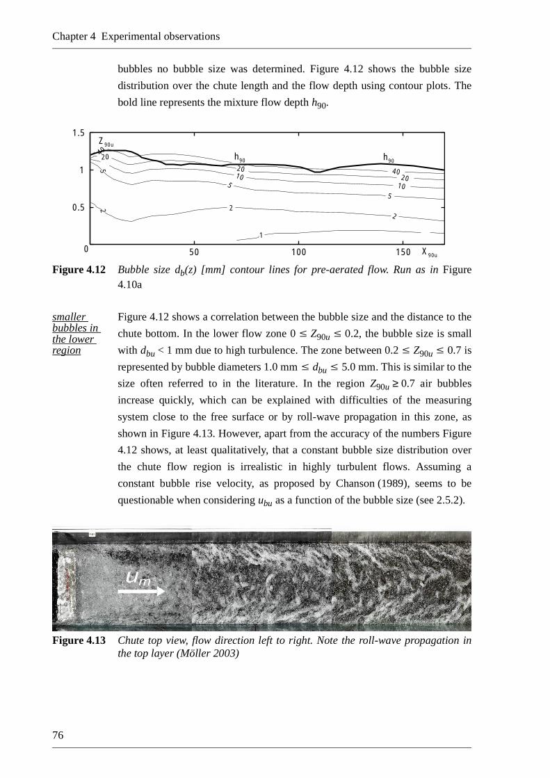
Chapter 4 Experimental observations
76
bubbles no bubble size was determined. Figure 4.12 shows the bubble size
distribution over the chute length and the flow depth using contour plots. The
bold line represents the mixture flow depth h90.
Figure 4.12 Bubble size db(z) [mm] contour lines for pre-aerated flow. Run as in Figure4.10a
smaller bubbles in the lower region
Figure 4.12 shows a correlation between the bubble size and the distance to the
chute bottom. In the lower flow zone 0 Z90u 0.2, the bubble size is small
with dbu < 1 mm due to high turbulence. The zone between 0.2 Z90u 0.7 is
represented by bubble diameters 1.0 mm dbu 5.0 mm. This is similar to the
size often referred to in the literature. In the region Z90u ≥ 0.7 air bubbles
increase quickly, which can be explained with difficulties of the measuring
system close to the free surface or by roll-wave propagation in this zone, as
shown in Figure 4.13. However, apart from the accuracy of the numbers Figure
4.12 shows, at least qualitatively, that a constant bubble size distribution over
the chute flow region is irrealistic in highly turbulent flows. Assuming a
constant bubble rise velocity, as proposed by Chanson (1989), seems to be
questionable when considering ubu as a function of the bubble size (see 2.5.2).
Figure 4.13 Chute top view, flow direction left to right. Note the roll-wave propagation inthe top layer (Möller 2003)
50 100 1500
0.5
1
1.5
1
2 22
5
5
5
1010
20
2020
40
40
X90u
Z90u
h90h90

Development of Aerated Chute Flow
77
CHAPTER 5 PRE-AERATED FLOW
5.1 Introduction
In the present project more than 150 experimental runs were conducted in the chute model.
This chapter presents the pre-aerated flow measurements where the air was added in the supply
pipe to obtain a hydraulically well defined two-phase flow at the jetbox. For systematical
investigations of the development of the average air concentration, the bottom air
concentration and the air detrainment gradient, the inflow Froude number, the chute slope, the
inflow depth, and the inflow air concentration was varied. It is further shown that the bubble
rise velocity depends on the air concentration. The streamwise development of average air
concentration can be divided into an air detrainment region, a minimum air concentration
region, an air entrainment region and an uniform flow region. The development depends on
hydraulic parameters such as streamwise Froude number, flow depth and chute slope.
5.2 Average air concentration
5.2.1 Typical air concentration development
streamwise average air concentra-tion C90 develop-ment
Hydraulic model tests were made to analyse the effect of hydraulic
parameters to the air-water flow field by a systematic variation of relevant flow
parameters. Figure 5.1 shows the typical average air concentration C90 defined
by equation (2.8) as a function of non-dimensional location X90u. The
streamwise average air concentration C90 decreases, starting from the inflow air
concentration Co, to a minimum Cmin. The average inflow air concentration Co
is influenced by the jetbox arrangement. The point of air inception X90u = Xi
was demonstrated to collapse with the point of minimum air concentration Cmin.
It is located where the local flow depth h = h(x) is equal to the thickness of
turbulent boundary layer δ = δ(x) (Vischer and Hager 1998).
inflow, minimum and uniform air concentra-tion
In the region downstream of Cmin air is entrained from the free surface
resulting in an increasing air concentration C90 up to an uniform average air
concentration C90u depending on the bottom slope only. All measurements
obeserved in the present project follow this typical development of average air
concentration. This section analyses the hydraulic influences on the curve
C90(X90u) by dividing it into several parts, namely: (1) Inflow air concentration

Chapter 5 Pre-aerated flow
78
region Co, (2) Air detrainment region C90,det, (3) Minimum air concentration
region Cmin, (4) Air entrainment region C90,ent, and (5) Uniform air
concentration region C90u (Kramer et al. 2004).
Figure 5.1 Typical average air concentration development C90 as a function ofnon-dimensional distance X90u
5.2.2 Effect of Froude number
average air concentra-tion curves
The effect of the Froude number was analysed using average air concentration
curves C90 for variable chute slopes, constant inflow depth and constant inflow
air concentration. Figure 5.2 shows the streamwise average air concentration
curves C90 as a function of non-dimensional location X90u for the four bottom
slopes So = 0 %, 10 %, 30 % and 50 %. All curves decrease first, starting at the
inflow air concentration Co to a minimum Cmin, as previously outlined. The
average minimum air concentration Cmin for steeper slopes So = 30 % and 50 %
is better defined than for So = 0 % and 10 %. On flat chutes, the minimum air
concentration in this study is defined at the break between the steep detrainment
curve and the downstream flow region where the air concentration curves
slightly decreases to attain the uniform average air concentration C90u. The
uniform average air concentration C90u at the downstream end of the channel as
shown in Figure 5.2 (a and b) depends on the water discharge Qw and the chute
slope So. It seems that for steeper slopes an equilibrium state is reached
depending on So only. Wood (1991) mentioned similar findings after
reinterpreting Straub and Anderson’s (1958) data. The region downstream of
the minimum air concentration is discussed in 5.2.9.
0 100 200
0.2
0.4
C90u
Cmin
C90Co
X90u
C90,det C90,ent
Xi
0.1
0.3

Development of Aerated Chute Flow
79
a) b)
c) d)
Figure 5.2 Average air concentration C90 as a function of non-dimensional distance X90u
for various slopes for a) So = 0 %, b) So = 10 %, c) So = 30 %, d) So = 50 %
5.2.3 Air detrainment region
average air concentra-tion reduces linearly
Figure 5.3 shows the same data as in Figure 5.2, where each measurement is
shifted from its first point at X90u = 0 in the x-direction on a generalized air
detrainment curve C90,det described by equation (5.2). The shifted distance
between the first point and the intersection with C90,det is
, (5.1)
depending on the inflow air concentration Co and the variable a. The average air
detrainment C90,det defines the reduction of the average air concentration C90
per chute length, e.g. X90u. Its best fit for the data in Figure 5.3 is
(5.2)
5.14 7.6910.0312.8013.62
0 100 200
0.2
0.4
C90u
Cmin
C90
Fo
Co
X90u
0.1
0.3
Fo
X90u
Cmin
C90u
Co
0 100 200
0.2
0.4C90
12.3813.6314.43
0.1
0.3
0 100 200
0.2
0.4
C90u
Cmin
C90
Fo
Co
X90u
5.11 7.7110.2811.5314.12
0.1
0.3
Fo 5.11
7.7110.2811.5314.12
C90u
Cmin
Co
Fo
0 100 200
0.2
0.4
X90u
C90
0.1
0.3
Xshi ftCo 0.40–( )
a---------------------------=
C90 det, aX90u c+=

Chapter 5 Pre-aerated flow
80
where a = f(So) < 0 and c = 0.40 is a constant. The parameter a varies between
-0.003 ≤ a ≤ -0.0017 for the four chute slopes investigated.
a) b)
c) d)
Figure 5.3 Average air detrainment C90,det as a function of non-dimensional distance X90u
for various slopes for data as in Figure 5.2, (---) equation (5.2), a) So = 0.0 %, a = –0.003, b) So = 10 %, a = –0.0028,c) So = 30 %, a = –0.0022, and d) So = 50 %, a = –0.0017
5.2.4 Effect of chute slope
air detrain-ment – a function of chute slope only
According to Figure 5.3 the average air detrainment is not only a function of the
inflow Froude number but of chute slope as well. Equation (5.2) involves
parameter a as a function of the chute angle α = arctanSo, with the sine defined
as sinα = So/(1+So2)1/2. Figure 5.4 shows this parameter as a function of chute
angle with the best fit (R2 = 0.98)
. (5.3)
Fo
X90u
Cmin
0 100 200
0.2
0.4C90,det
Xshift
5.14 7.6910.0312.8013.62
0.1
0.3
Fo
X90u
Cmin
0 100 200
0.2
0.4
12.3813.6314.43
C90,det
Xshift
0.1
0.3
Fo
X90u
Cmin
0 100 200
0.2
0.4C90,det
Xshift
5.11 7.7110.2811.5314.12
0.1
0.3
Fo
X90u
Cmin
0 100 200
0.2
0.4C90,det
Xshift
5.11 7.7110.2811.5314.12
0.1
0.3
a 0.003 α 1–sin( )=
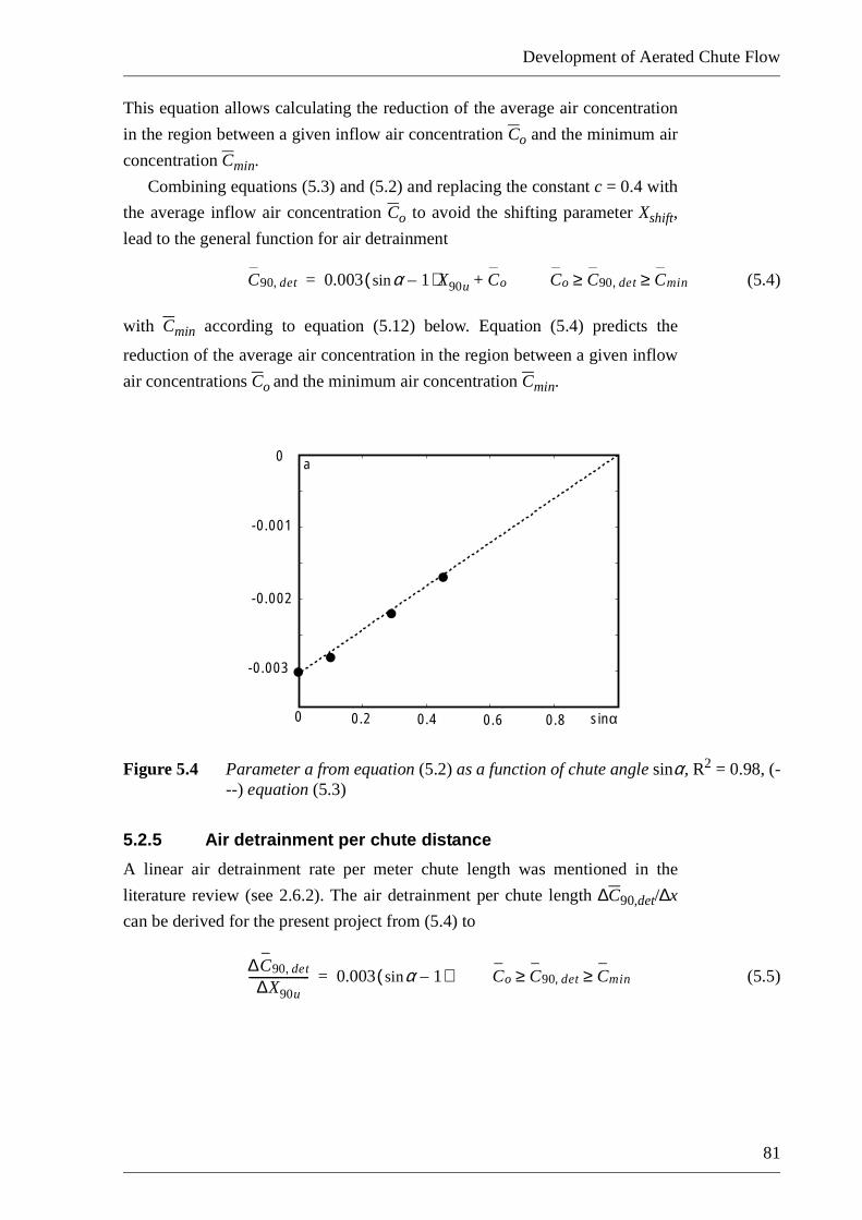
Development of Aerated Chute Flow
81
This equation allows calculating the reduction of the average air concentration
in the region between a given inflow air concentration Co and the minimum air
concentration Cmin.
Combining equations (5.3) and (5.2) and replacing the constant c = 0.4 with
the average inflow air concentration Co to avoid the shifting parameter Xshift,
lead to the general function for air detrainment
(5.4)
with Cmin according to equation (5.12) below. Equation (5.4) predicts the
reduction of the average air concentration in the region between a given inflow
air concentrations Co and the minimum air concentration Cmin.
Figure 5.4 Parameter a from equation (5.2) as a function of chute angle sinα, R2 = 0.98, (---) equation (5.3)
5.2.5 Air detrainment per chute distance
A linear air detrainment rate per meter chute length was mentioned in the
literature review (see 2.6.2). The air detrainment per chute length ∆C90,det/∆x
can be derived for the present project from (5.4) to
(5.5)
C90 det, 0.003 αsin 1–( )X90u Co+= Co C90 det, Cmin≥ ≥
0
sinα0.2 0.4 0.6 0.8
0
-0.001
-0.002
-0.003
a
∆C90 det,∆X90u
--------------------- 0.003 α 1–sin( )= Co C90 det, Cmin≥ ≥

Chapter 5 Pre-aerated flow
82
and thus to
. (5.6)
Example 5.1Problem: Consider a typical chute for various chute slopes So = 10 %, 20 %, 30 %, 40 % and
50 %, for a water discharge Qw = 3000 m3/s, a chute width b = 40 m, and a surfaceroughness height kst = 90 m1/3/s. Assume a wide chute for which Rh ≈ hw, and calculatethe flow field for pure water only. Find a) the uniform flow depths h90u ≈ hw, and b) theair detrainment ∆C90,det per chute meter ∆x = 1 m.
Solution: The uniform flow depth can be calculated using the Manning-Strickler equation forwide rectangular chutes h90u = hw = [Qw
2/(sinαkst2b2)]3/10 according to equation (5.7).
Equation (5.6) gives ∆C90,det.Answer: Table 5.1 shows the solution. Note that ∆C90,det is only applicable for
Co ≥ C90,det ≥ Cmin! There is a surprising agreement between the results in Table 5.1,with –0.15 %/m ≤ ∆C90,det/m ≤ –0.17 %/m, and the results found on prototypespillways between –0.10 %/m ≤ ∆C90,det/m ≤ –0.20 %/m (Prusza 1983, andMinor 2000).
Table 5.1 Air detrainment ∆C90,det per meter chute length
Air detrainment per meter
air detrain-ment per chute meter
Equation (5.6) is a function of the chutes angle sinα and the uniform mixture
flow depth h90u which depends on the chute angle too. The uniform flow depth
in equation (5.6) may be substituted by the Manning-Strickler equation
v = kst2RhSo
1/2. The Manning-Strickler formula is based on the Chezy formula
substituting the Chezy number C with the empirical kst number. The original
Chezy formula, used for the equilibrium of forces, was based on the chute angle
sinα instead of the tanα. Due to simplifications the tanα was used for the
Manning-Strickler formula, which is acceptable for small chute slopes. For
So= atanα 10 % 20 % 30 % 40 % 50 %
sinα 0.10 0.20 0.29 0.37 0.45
h90u = hw 1.79 m 1.45 m 1.29 m 1.18 m 1.10 m
∆C90,det/∆x –0.151 %/m –0.166 %/m –0.166 %/m –0.160 %/m –0.150 %/m
∆C90 det,∆x
---------------------0.003 α 1–sin( )
h90u--------------------------------------= Co C90 det, Cmin≥ ≥

Development of Aerated Chute Flow
83
steeper slopes, one must substitute the chute slope So = tanα with the sine of the
chute angle sinα. Furthermore, assuming a wide channel wiht Rh ≈ hw and a
flow velocity v = Qw/(b•hw), the transposed Manning-Strickler leads to
(5.7)
substituting (5.7) to equation (5.6) leads to
(5.8)
with the specific discharge qw = Qw/b. A classical curve sketching shows that
equation (5.8) has two zeros for sinα = 0 and 1 meaning that no air detrains for
horizontal and vertical chute slopes. Note that the horizontal slope is a rather
academic example because the specific discharge would entail an infinite
uniform flow depth. Further, the function has a minimum for
(5.9)
where the air detrainment is maximal. According to Figure 5.5, the maximum
air detrainment, is in the region where the curve has its minimum. This
minimum may be defined for the region between 0.09 ≤ sinα ≤ 0.45. The
maximum air detrainment per chute meter depends on kst and qw only, when a
constant detrainment rate is assumed of
. (5.10)
h90u
Qw2
αsin kst2
b2
------------------------
310------
=
∆C90 det,∆x
--------------------- 0.003kst
qw------
35---
αsin( )310------
αsin 1–( )=
αsin313------ 0.23 α 13.3°= = =
∆C90 det,∆x
---------------------
max0.00– 15
kst
qw------
35---
= 0.09 αsin 0.45≤ ≤

Chapter 5 Pre-aerated flow
84
Figure 5.5 Air detrainment ∆C90,det per chute distance ∆x, as a function of chute angle α,(–––) equation (5.8), almost constant maximum detrainment zone
Example 5.2Problem: Consider the spillway again (Example 5.1). Find the maximum air detrainment rates
per chute meter for specific discharges 40 m2/s≤ qw ≤ 140 m2/s with (∆C90,det/∆x)max = –0.0015(kst/qw)3/5, for a chute of slope So = 40 % and kst = 90 m1/3/s.
Solution: The maximum air detrainment rate can be calculated using ∆C90,det/∆x = –0.0015(kst/qw)3/5 according to equation (5.10).
Answer: Table 5.2 shows that this solution may be applied on chutes with 0.09 ≤ sinα ≤ 0.45(0.09 ≤ So ≤ 0.50).
Table 5.2 Maximum air detrainment per meter (∆C90,det/m)max depending on the specific
discharge qw
Table 5.2 recommends that the average air detainment per chute meter
decreases with a higher specific discharge qw. This is due to the relative
reduction of the surface roughness ks with increasing flow depth. Hence,
turbulent effects lessen relatively with higher discharges, causing a somewhat
smaller influence to the air bubble motion.
qw 40 m2/s 60 m2/s 80 m2/s 100 m2/s 120 m2/s 140 m2/s
(∆C90,det/∆x)max
–0.24 %/m –0.19 %/m –0.16 %/m –0.14 %/m –0.13 %/m –0.12 %/m
0
sinα0.2 0.4 0.6 0.8
0
-0.0005
-0.0010
-0.0015
∆C90,det
∆x(ks/qw)3/5

Development of Aerated Chute Flow
85
5.2.6 Minimum average air concentration
minimum air concentra-tion – a function of Froude number and flow depth
The minimum average air concentration Cmin is an important parameter for
protection of chutes against cavitation damage. It was found to be a function of
chute bottom slope, mixture flow depth and streamwise Froude number. The
streamwise Froude number development depends directly on the flow depth
which again depends on the bottom slope; the unknown function may thus be
expressed as Cmin = f(F(x)). It was found that the overall flow development is
more important than inflow or uniform conditions.
the turbulent boundary layer influences the minimum air concentra-tion
The turbulent boundary is assumed to reach the free surface where the
thickness of the boundary layer is equal to the inception flow depth δ = hi, it is a
function of the surface roughness height ks, the difference of water elevation
between the inception point and the reservoir level Hs, the critical flow depth hc
and the chute slope So, as mentioned in 2.4.2. The streamwise development of
the thickness of the boundary layer is independent of the flow depth, thus larger
hi entail larger xi. Minimum air concentration is consequently reached further
downstream for larger then for smaller flow depths (see 5.2.7).
The best feasable description of the general flow development for the
minimum air concentration was found to be the arithmetic average of the inflow
Froude number Fo and the Froude number at the inception point F(Cmin) to be
. (5.11)
Figure 5.6a shows the minimum air concentration plotted against the average
streamwise Froude number Fo-min for all measurements with So ≥ 10 %. The
best fit was found to
. (5.12)
the upstream develop-ment is found to be the important factor
The correlation yields R2 = 0.56 which is poor due to the data with small inflow
Froude numbers. For inflow Froude numbers Fo ≥ 7 and bottom slopes
So ≥ 10 % the correlation increases to R2 = 0.85 (Figure 5.6b). For small bottom
slopes no free surface air entrainment occurs and the air concentration falls
finally to zero. For Froude numbers Fo-min ≥ 10, the average minimum air
concentration never fell below Cmin = 0.15.
Fo min–
Fo F Cmin( )+
2--------------------------------=
Cmin 0.015Fo m– i n=

Chapter 5 Pre-aerated flow
86
a) b)
Figure 5.6 Minimum air concentration Cmin against streamwise Froude number Fo-min for
So ≥ 10 %; a) all data, correlation R2 = 0.56, b) data for Fo ≥ 7, correlation
R2 = 0.85
5.2.7 Effect of inflow depth
the average air detrain-ment is not influenced by the inflow depth
The inflow flow depth ho was varied between 0.03 m ≤ ho ≤ 0.11 m. The
Froude number was computed using the water discharge which was limited to
Qw = 250 l/s, and the air discharge limited to Qa = 55 l/s. Figure 5.7 shows, as
an example, the effect of the inflow depth on the air detrainment of the average
air concentration C90 for the chute slope So = 30 %. The air concentration
reduces, similarly to the measurement shown in Figure 5.3c with a constant
flow depth ho = 0.06 m, except for ho = 0.11 m which corresponds to Fo = 3.91.
It was found that Froude numbers below Fo ≤ 4 result in poor correlation again
and are therefore not shown. For the horizontal chute Fo ≤ 6 data were not
representative due to limited air presence. Because cavitation occurs for high
flow velocities associated with high Froude numbers, small Froude numbers
below Fo ≤ 4 were considered insignificant for all further evaluations. The
remaining measurements shown in Figure 5.7 follow the same trend as in Figure
5.3. Hence, measurements with a constant inflow depth for inflow Froude
numbers exceeding ho = 0.05 m and Fo = 4 are adequate for the data analysis.
5.14 0.05 0.10 7.69 0.05 0.1010.03 0.05 0.1012.80 0.05 0.1013.62 0.05 0.10 8.60 0.06 0.1010.41 0.06 0.1011.68 0.06 0.10 9.41 0.06 0.1011.34 0.06 0.10 5.11 0.06 0.30 7.71 0.06 0.3010.28 0.06 0.3011.53 0.06 0.3014.15 0.05 0.30 5.14 0.10 0.30 7.60 0.08 0.3010.19 0.07 0.30 5.11 0.06 0.50 7.71 0.06 0.5010.28 0.06 0.5011.53 0.06 0.5014.12 0.05 0.50 5.14 0.10 0.50 7.60 0.08 0.50
Fo ho SoCmin
10 200
0.1
0.2
0.3
Fo-min
7.69 0.05 0.1010.03 0.05 0.1012.80 0.05 0.1013.62 0.05 0.10 8.60 0.06 0.1010.41 0.06 0.1011.43 0.06 0.10 9.41 0.06 0.1011.34 0.06 0.10 7.71 0.06 0.3010.28 0.06 0.3011.53 0.06 0.3014.15 0.05 0.30 7.60 0.08 0.3010.19 0.06 0.30 7.71 0.06 0.5010.28 0.06 0.5011.53 0.06 0.5014.12 0.05 0.50 7.60 0.08 0.5010.28 0.06 0.50
Fo ho So
Cmin
10 200
0.1
0.2
0.3
Fo-min

Development of Aerated Chute Flow
87
Figure 5.7 Average air detrainment C90 as a function of non-dimensional distance X90u forvarious flow depths 0.05 m ≤ ho ≤ 0.11 m, 0.18 ≤ β ≤ 0.22, and So = 30 % (---)equation (5.2)
5.2.8 Effect of inflow air concentration
inflow air concentra-tion β has no meaningful influence on the distance protected
The variation of the inflow air concentration β was considered important for the
distance to be protected against cavitation damage by air addition. Most design
guidelines (see 2.6.2) are based on the inflow air concentration. However,
Oskolov and Semenkov (1979) demonstrated that a maximum average air
concentration above 45 % result in over-saturation of the flow because a higher
concentration would produce mainly spray. Figure 5.8a shows that the average
inflow air concentration Co varies with the amount of added air Qa. For Co ≥ 0.4
the air detrains rather quickly. The inflow air concentration appears to be not the
determining factor for the distance to be protected by air because all
measurements result in about the same minimum air concentration Cmin at
X90u ≈ 50. The air supplied detrains immediately if the amount of air exceeds
the transport capacity of the flow. Whereas Figure 5.8b shows that the
measurements are almost parallel for Co ≤ 0.4 and can thus be calculated by
equation (5.1). It can therefore be concluded that the flow transport capacity is
more important for the streamwise air concentration capacity than the absolute
amount of air supplied.
X90u
Cmin
0 100 200
0.2
0.4C90
Xshift
Fo ho
3.91 0.110 5.14 0.100 7.60 0.08010.19 0.06511.53 0.06014.12 0.050
0.1
0.3

Chapter 5 Pre-aerated flow
88
a) b)
Figure 5.8 Average air concentration C90 as a function of non-dimensional distance X90u
for various chute slopes, a) So = 0.0 %, 0.19 ≤ β ≤ 0.28, b) So = 10 %,0.20 ≤ β ≤ 0.30
Example 5.3
Problem: Consider a chute model of chute slope So = 30 %, water discharge Qw = 198 l/s, inflowair concentration Co = 0.30, inflow depth ho = 0.07 m, and flow depth at the point ofinception h(Cmin) = 0.05 m. a) Find the average minimum air concentration Cmin andthe corresponding location X90u of Cmin. b) Determine the distance between the airsupply and the minimum air concentration.
Solution: Calculating Fo = 0.198/(9.81•0.52•0.073)0.5 = 6.83 and F(Cmin) = 0.198/(0.52•9.81•0.053)0.5 = 11.31 by equation (3.1), the streamwise average Froude numberis Fo-min = (6.83 + 11.31)/2 = 9.07 using equation (5.11). According to equation (5.12)and Figure 5.6, Cmin = 0.015•9.07 = 0.14 = 14 %. Using equation (5.3) or Figure 5.4gives a = 0.003(0.29 – 1) = –0.0021. Arranging equation (5.2) for X90u, withC90,det = Cmin = 0.14, results in X90u = 119.0, or with Figure 5.3, equation (5.1) resultsin Xshift = –47.6 with respect to the inflow air concentration.
Answer: a) The minimum average air concentration is Cmin = 0.14 = 14 %, b) the distance fromthe air supply to the minimum air concentration is X90u = X90u + Xshift = 71.7 (Figure5.3c). Equation (5.4) may also be used for calculating the streamwise reduction of theair concentration.
5.2.9 Air entrainment region
air detrain-ment, minimum air concentra-tion and air entrain-ment
Two important effects for the average air concentration C90 where described in
the previously chapters, namely: (1) The average air detrainment curve depends
on the inflow air concentration Co and the bottom slope So, and (2) The
minimum air concentration Cmin depends on a combination of the inflow
Froude number Fo and the local Froude number at the point of inception
F(Cmin). For cavitation protection of a chute the distance to the next aerator
8.60 0.30 9.41 0.2610.41 0.2311.34 0.2111.68 0.20
X90u
Cmin
C90u
Co
0 100 200
0.2
0.4C90
Fo βo
0.1
0.3
7.40 0.28 9.94 0.2312.38 0.1913.63 0.1914.43 0.19
X90u
Cmin
C90u
Co
0 100 200
0.2
0.4C90
Fo βo
0.1
0.3
Development of Aerated Chute Flow
89
results from the above proposed equations (5.12) and (5.4), provided the
minimum average air concentration required for spillway protection is known
(Example 5.3).
Ehrenberger (1926) established that air in high-speed chute flows is
entrained by free surface aeration. The free surface aeration is an important
feature for aerator spacing because downstream of the inception point no
additional aerator is normally needed. The average air concentration in uniform
mixture flow was considered by, e.g. Hager (1991) who stated that C90u
depends on the chute slope only, based on Straub and Anderson’s (1958)
classical data set. The streamwise development of average air concentration for
chute flows was investigated by Kramer et al. (2003). Figure 5.9a shows, as an
example, the effect of free surface aeration by means of air contour lines. Here,
the air contour lines C(x) show a steep gradient between the free surface C = 1
and black water C = 0 at the jetbox for X90u = 0, which means almost pure water
flow at this point. The jetbox has, however, a somewhat roughening effect to the
flow surface. The air concentration contours C(x) dowstream of the jetbox show
a fan-shaped behaviour where the C = 0.001 impinges the chute bottom at
X90u ≈ 200.
comparing pre-aerated and non-aerated flow
Figure 5.9b shows the streamwise development of average air concentration
C90 for two otherwise identical experiments, for pre-aerated jetbox flow with
β = 21 %, and for non-aerated inflow with β = 0 %, respectively. Note the
linear increase of the average air concentration for non-aerated inflow which
proves that surface air entrainment is important. Note also the almost identical
uniform air concentrations at the downstream side of the two respective plots.
general air entrain-ment function
The curve for the pre-aerated measurement in Figure 5.9b increases
significantly shortly downstream of the jetbox X90u ≤ 10 to the inflow air
concentration of Co = 0.27, and then decreases, as previously explained.
Additionally, Figure 5.9b shows that the air entrainment for pre-aerated flow
downstream of the minimum air concentration Cmin increases more gently
compared to non-aerated flow, but finally reaches about the same uniform air
concentration C90u = 0.29 as can be shown later (Figure 5.10c and d).

Chapter 5 Pre-aerated flow
90
a) b)
Figure 5.9 a) Contour plot for non-aerated flow Fo = 7.71, So = 50 %, shock wave,b) Average air concentration C90 as a function of non-dimensional distanceX90u for pre-aerated flow with β = 21 % and non-aerated inflow,respectively, (-.-.-) uniform air concentration. Run as in a)
the general equation depends on the uniform air concentra-tion only
The process of air entrainment was analysed for the region between the average
minimum air concentration Cmin and the uniform air concentration C90u. Figure
5.10a-c show the air entrainment downstream of the point of minimum air
concentration for various chute slopes. For the horizontal chute So = 0 no air
entrainment at all was observed. The measurements were shifted in the same
way as explained in 5.2.3 on equation (5.13) based on the minimum air
concentration. This method enables to compare the air entrainment for different
measurements independent of the minimum air concentration. The best analytic
fit for the average air entrainment was found to be the hyperbolic tangent
function
(5.13)
with C90u = f(So) (Figure 5.10) and d = 0.004 for pre-aerated, and d = 0.006 for
non-aerated inflow conditions. The general form of this equation with d = 0.004
depends on the uniform air concentration C90u only. Two outliers are notable in
Figure 5.10c and one in Figure 5.10d relating to the data sets with the smallest
discharges. Both data sets appear to deviate from the general trend at their ends,
because of a sudden increase of C90. These data points are affected from model
limitations. For flow depths reducing below hw ≈ 2 cm the single measuring
steps between two points in vertical direction ∆z ≈ 0.20 mm are to large to
define a clear boundary. Additionally, minute shock waves have relatively
C90u
X90u0 100 200
0.2
0.4C90
Cmin
Co 1
2
10
0.1
0.3
0 100 200
0.5
1
1.5
0.001
0.001
0.01
0.05 0.1
0.5
0.90.95
0.990.99
0.50.1
Z90u
X90u
free surface aeration
C90 ent, C90utanh d X90u⋅( )=

Development of Aerated Chute Flow
91
larger influences to these observations. However, these three data points seem
not to have an influence on the general trend line and are specially marked in
Figure 5.10c and d, respectively.
a) b)
c) d)
Figure 5.10 (–––) Average air entrainment C90,ent for jetbox flow according to equation(5.13) as a function of non-dimensional distance X90u for various chute slopesfor a) So = 10 %, C90u = 0.20, b) So = 30 %, C90u = 0.23, c) So = 50 %,C90u = 0.29, and d) for non-aerated jetbox flow with So = 50 %, C90u = 0.29
comparing the present data to that in the literature
Equation (5.13) describes a general form of the air entrainment function
depending on the average air concentration in the equilibrium state. It was
shown by Hager (1991), who mentioned C90u = 0.75(sinα)0.75 (equation
(2.14)), and Chanson (1997), who stated C90u = 0.90sinα (equations (2.15)), in
2.4.2 that the uniform air concentration C90u varies with the bottom slope only.
Both statements are based on Straub and Anderson’s (1953) results. It was
attempted to confirm the two equations even if the chute roughness differed
3.99 5.14 7.60 7.7110.1910.2811.5314.12
X90u
Cmin
C90u
(30%)=0.23
0 200 400
0.2
0.4C90,ent
Fo
0.1
0.3
8.60 9.4110.4111.3411.6812.8013.62
X90u
Cmin
C90u
(10%)=0.20
0 200 400
0.2
0.4C90,ent
Fo
0.1
0.3
4.006.008.009.3211.00
X90u
Cmin
C90u
(50%)=0.29
0 200 400
0.2
0.4C90,ent
Fo
scale effect
0.1
0.3
5.11 5.11 7.60 7.7110.1910.2811.5314.12
X90u
Cmin
C90u
(50%)=0.29
0 200 400
0.2
0.4C90,ent
Fo
scale effect
0.1
0.3
Chapter 5 Pre-aerated flow
92
strongly from the present roughness. Figure 5.11a shows the air entrainment
concentration C90,ent as a function of X90u for the four investigated chute slopes
So, based on Figure 5.10 and equation (5.13), respetively. The influence of the
bottom slope on the uniform air concentration is obvious, with higher uniform
average air concentration for steeper slopes.
lower air concentra-tions in the present project
Figure 5.11b compares C90u from the present project with proposals by
Hager and Chanson applying Straub and Anderson’s data. The equilibrium or
uniform flow region was not focused in the present project due to the limited
chute length of l = 14 m, for chute slopes So ≤ 50% and constant roughness
ks = 0.00023 mm (see 3.4.3). Anderson (1965) added smooth channel
measurements but did not publish the entire data set. Therefore, only uniform
average air concentrations integrated over the flow depth h99 instead of the h90
standard are available. Anderson (1965) mentioned that further experimentation
in this area is necessary to delineate the transition from the air-water mixture in
the smooth to the rough chute. Lakshmana Rao and Kobus (1973) added data
for C99u but did not publish detailed measurements. The large deviations
between those from the present data sets can be traced back to the effect of
surface roughness. Whereas Straub and Anderson used an artificially roughened
surface, the present project was based on a practically smooth boundary surface.
This effect needs additional attention in the future.
air entrain-ment function
A limited amount of average air concentration data in the uniform region is
available in the present project, of which best fit is (Figure 5.11b)
(5.14)
with a correlation coefficient of R2 = 0.98. Combining equations (5.13) and
(5.14) thus gives
(5.15)
with d = 0.004 for 0 ≤ So ≤ 50% and hydraulic smooth, pre-aerated inflow
conditions. The effect of bottom slope is relatively small for So ≥ 10 %, whereas
air entrainment increases significantly for C90 ≤ 2/3C90u.
C90u13--- αsin( )0.25
= 0 αsin 0.5≤ ≤
C90 ent,13--- αsin( )0.25
tanh d X90u⋅( )=

Development of Aerated Chute Flow
93
a) b)
Figure 5.11 a) Streamwise average air entrainment C90,ent for various bottom slopes, (–––)equation (5.13), b) uniform air concentration C90u as a function of bottom slope
sinα = So/(1 + So)0.5, (–––) equation (5.14) with R2 = 0.98, (---) equation(2.14) by Hager (1991), and (-.-.-) equation (2.15) by Chanson (1997)
Example 5.4
Problem: Consider the flow given by Example 5.3. Calculate the streamwise behaviour of theaverage air concentration downstream of the point of inception C90,ent (point ofminimum air concentration).
Solution: According to equation (5.14), the uniform air concentration is C90u = 1/3(0.29)0.25 = 0.24.
Answer: The streamwise development of the air entrainment downstream of the point ofinception can be described as: C90,ent = 0.24tanh(0.004X90u) using equation (5.13) or(5.15) or Figure 5.11.
5.3 Bottom air concentration
5.3.1 Effect of Froude number
bottom air concentra-tion
The bottom (subscript b) air concentration Cb is relevant for chute cavitation
protection, even if there is still an ongoing discussion on the amount of air
required for adequate chute surface protection (see 2.3.2). The bottom air
concentration Cb is examined in a similar way as was the average air
concentration C90.
Figure 5.12 shows streamwise bottom air concentration Cb as a function of
X90u in a semi-logarithmic plot for four different bottom slopes So = 0 %, 10 %,
30 % and 50 %, and Froude numbers 4.5 ≤ Fo ≤ 14.4. Close to the jetbox
X90u ≈ 0 air concentrations were close to Cbo ≈ 5 %. This is a characteristic
value of bottom air concentration generated by the jetbox for pre-aerated flow
conditions independent of Co. Compared to the average air concentration where
X90u
C90u
(50%)=0.29
0 200 400
0.2
0.4C90,ent
C90u
(30%)=0.23
C90u
(10%)=0.20
C90u
(0%)=0.0
0.1
0.3
sinα0 0.4 0.8
0.2
0.6
0.4
C90u
C90u
=0.33(sinα)0.25
C90u
=0.75(sinα)0.75
C90u
=0.9sinα

Chapter 5 Pre-aerated flow
94
the jetbox entrains air similar to a bottom outlet gate, the bottom air
concentrations is not influenced from the opening. No air concentration
information can be deduced with the fiber-optical measuring system for
concentrations falling below Cb = 0.0001 (see 3.4.2), but this occurs mainly for
flows with small Froude numbers far downstream of the chute.
the same three regions as for average air concentra-tion
The data of Figure 5.12 can be classified in the same three regions as for the
average air concentration, namely: (1) Air concentration decay in the near flow
field, (2) Minimum value region, and (3) Increasing air concentration region. It
is assumed that the air entrained from the free surface has not reached the
bottom sustainable to obtain equilibrium conditions due to limited channel
length. The inflow Froude number Fo is the major factor for the streamwise
development of the bottom air concentration. All curves start at the
characteristic value of bottom air concentration at the inflow Cbo, decrease
fan-shaped in the semi-logarithmic plot, depending on the inflow Froude
number. The bottom slope has two effects: (1) The gradient of the decreasing
curves Cb,det depends on the bottom slope, and (2) The kink in the detrainment
curves (Figure 5.12c and d) between the steep and the flatter decay regions is
better defined for steep than for flat slopes, whereas the air concentration
reduces to zero further downstream for almost horizontal chutes.
a) b)100 200
X90u100 200
Cb Fo 8.3810.3812.3813.6314.43
Cb = 1 %
10-4
10-3
10-2
10-1
1
Cbo
0
X90u100 200
Cb
Cb = 1 %
10-4
10-3
10-2
10-1
1 5.14 7.6910.0312.8013.62
Fo
Cbo
0

Development of Aerated Chute Flow
95
c) d)
Figure 5.12 Bottom air concentration Cb as a function of non-dimensional distance X90u forvarious slopes a) So = 0 %, b) So = 10 %, c) So = 30 %, and d) So = 50 %
5.3.2 Air detrainment region
bottom air concentra-tion reduces semi-logarithmic
Figure 5.13 shows the identical data as in Figure 5.12 for the air detrainment
portion. The semi-logarithmic, fan-shaped form is exposed by lines following
the detraining trend. The gradient of each line depends on the inflow Froude
number Fo as
(5.16)
where Cbo is the upstream bottom air concentration.
a) b)
X90u100 200
Cb Fo
Cb = 1 %
10-4
10-3
10-2
10-1
1 5.11 7.7110.2811.5314.12Cbo
0
X90u100 200
CbFo
Cb = 1 %
10-4
10-3
10-2
10-1
1 5.11 7.7110.2811.5314.12Cbo
0
Cb det, Cboem– X90u=
100 200
X90u100 200
Cb,det Fo m 8.38, 0.08010.38, 0.03612.38, 0.02513.63, 0.01814.43, 0.015
Cb = 1 %
10-4
10-3
10-2
10-1
1
Cbo
m
X90u100 200
Cb,det
Cb = 1 %
10-4
10-3
10-2
10-1
1
Cbo
7.69, 0.06610.03, 0.03112.80, 0.016
Fo m 5.14, 0.163
13.62, 0.013

Chapter 5 Pre-aerated flow
96
c) d)
Figure 5.13 Bottom air concentration Cb,det in the detrainment region as a function of non-dimensional distance X90u for various bottom slopes a) So = 0 %, b) So = 10 %,c) So = 30 %, and d) So = 50 %, (–––) slope m for (5.16)
The best fit for the air detrainment gradient m= f(Fo) as a function of the inflow
Froude number is
(5.17)
Cb,det depends on the Fo
with n = f(So). Equation (5.17) implies that the bottom air detrainment gradient
can be approximated with a power function where the inflow Froude number
dominates. Figure 5.14 shows that n in equation (5.17) depends exclusively on
the chute bottom slope with n ranging between 7.18 ≤ n ≤ 14.42.
a) b)
X90u100 200
Cb,det
Cb = 1 %
10-4
10-3
10-2
10-1
1
Cbo
7.71, 0.03710.28, 0.02311.53, 0.021
Fo m 5.11, 0.155
14.12, 0.012
X90u100 200
Cb,det
Cb = 1 %
10-4
10-3
10-2
10-1
1
Cbo
7.71, 0.04410.28, 0.01811.53, 0.015
Fo m 5.11, 0.122
14.12, 0.012
m nFo2.50–
=
0 5 10
0.2
0.4
Fo
mm = 14.42Fo
-2.50
0 5 10
0.2
0.4
Fo
mm = 9.88Fo
-2.50

Development of Aerated Chute Flow
97
c) d)
Figure 5.14 Bottom air detrainment gradient m as a function of inflow Froude number Fo
for
a) So = 0 %, n = 14.42, R2 = 0.99, b) So = 10 %, n = 9.88, R2 = 0.99,
c) So = 30 %, n = 8.79, R2 = 0.97, and d) So = 50 %, n = 7.18, R2 = 0.99,(–––) according to equation (5.17)
5.3.3 Effect of chute slope
bottom air detrain-ment – a function of bottom slope and inflow Froude number
Equation (5.17) suggests a method to calculate the bottom air detrainment
gradient by means of a power function. The equation was derived for constant
chute slopes with variable inflow Froude numbers including a variable n as a
function of chute slope. Figure 5.15a shows all corresponding curves m = f(Fo)
developed from Figure 5.14. A large detrainment gradient for Froude numbers
Fo ≤ 5 was observed for all bottom slopes, whereas the bottom slope has no
major influence on the detrainment gradient for Fo ≥ 12. According to Figure
5.15b n ranges between 7.18 ≤ n ≤ 14.42 for chute slopes So ≤ 50 %. The
variable n varies as n = f(Fo, So), therefore. The best fit for the variable n as a
function of chutes slope is (R2 = 0.94)
. (5.18)
A combination of equations (5.16), (5.17) and (5.18) results in the general
equation for the bottom air detrainment
. (5.19)
0 5 10
0.1
0.2
Fo
m = 8.79Fo
-2.50
m
0 5 10
0.1
0.2
Fo
mm = 7.18Fo
-2.50
n 7.2 0.006So 6.6+⋅=
Cb det, Cboe7.2 0.006
So 6.6+⋅( )– Fo2.50– X90u= Cbo Cb det, Cb min,≥ ≥

Chapter 5 Pre-aerated flow
98
a) b)
Figure 5.15 a) Superposition of curves m = f(Fo) from Figure 5.14 for all bottom slopes,
b) parameter n from Figure 5.15a as a function of chute slope So, R2 = 0.94
high quality of equation (5.19)
Equation (5.19) predicts the detrainment of the bottom air concentration Cb,det
of pre-aerated jetbox flow between the inflow bottom air concentration Cbo and
the minimum bottom air concentration Cb,min. The quality of equation (5.19) is
shown in Figure 5.16 where the trend lines are compared to the original data
from Figure 5.13. In Figure 5.16, the continuous lines are the predicted bottom
air concentration according to equation (5.19), up to the minimum Cb,min where
the continuous line changes to a dashed line. The thin dotted lines represent the
trend lines from Figure 5.13 which were taken to be the best fit for the bottom
air detrainment measurements. Note the small deviations between the
continuous lines and the dotted lines.
a) b)
0
n = 7.2•0.006So + 6.6
So0.4 0.8
30 n
15
So = 0.0 %
So = 10 %
So = 30 %
So = 50 %
0 5 10
0.2
0.4
Fo
mm = nFo
-2.50
X90u100 200
Cb,det Fo 8.3810.3812.3813.6314.43
Cb = 1 %
10-4
10-3
10-2
10-1
1
X90u100 200
Cb,det
Cb = 1 %
10-4
10-3
10-2
10-1
1 5.14 7.6910.0312.8013.62
Fo
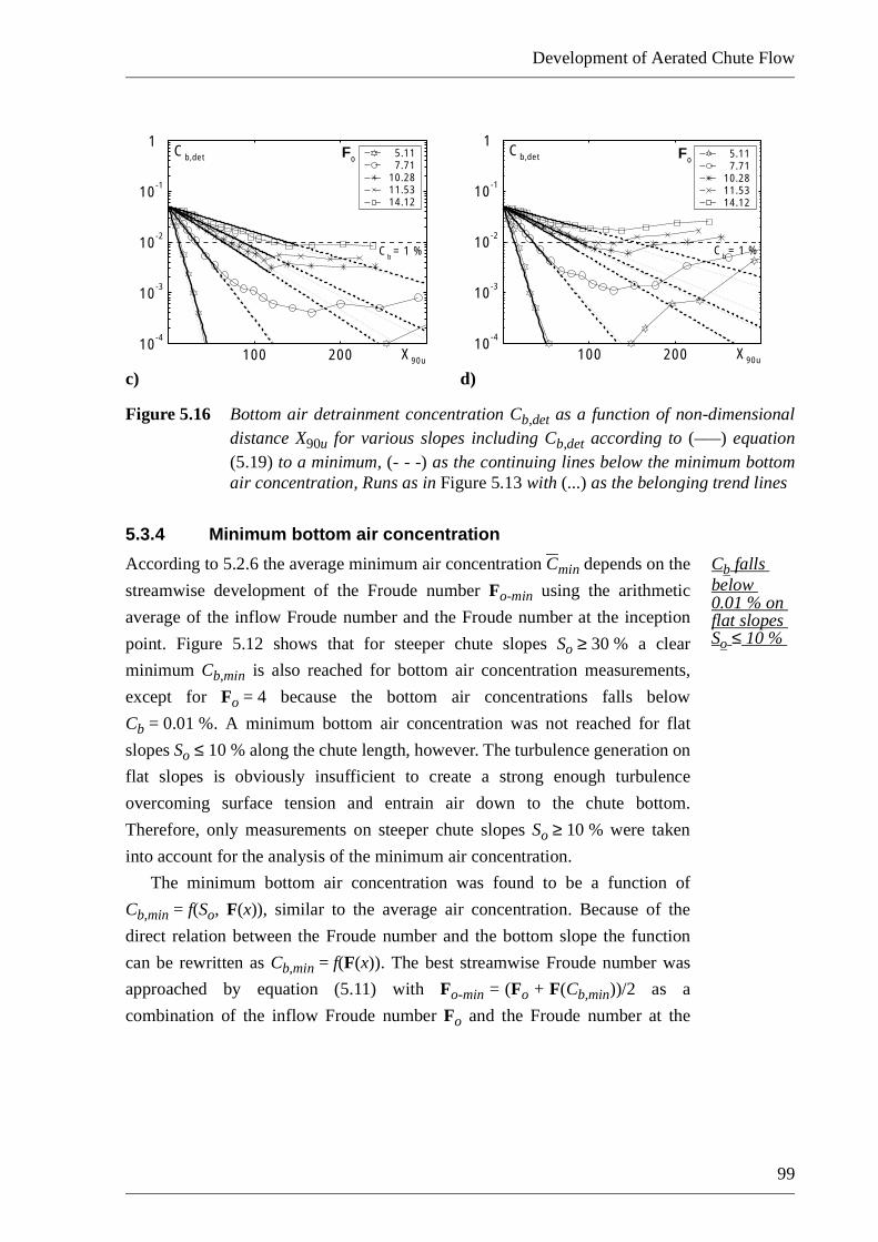
Development of Aerated Chute Flow
99
c) d)
Figure 5.16 Bottom air detrainment concentration Cb,det as a function of non-dimensionaldistance X90u for various slopes including Cb,det according to (–––) equation(5.19) to a minimum, (- - -) as the continuing lines below the minimum bottomair concentration, Runs as in Figure 5.13 with (...) as the belonging trend lines
5.3.4 Minimum bottom air concentration
Cb falls below 0.01 % on flat slopes So ≤ 10 %
According to 5.2.6 the average minimum air concentration Cmin depends on the
streamwise development of the Froude number Fo-min using the arithmetic
average of the inflow Froude number and the Froude number at the inception
point. Figure 5.12 shows that for steeper chute slopes So ≥ 30 % a clear
minimum Cb,min is also reached for bottom air concentration measurements,
except for Fo = 4 because the bottom air concentrations falls below
Cb = 0.01 %. A minimum bottom air concentration was not reached for flat
slopes So ≤ 10 % along the chute length, however. The turbulence generation on
flat slopes is obviously insufficient to create a strong enough turbulence
overcoming surface tension and entrain air down to the chute bottom.
Therefore, only measurements on steeper chute slopes So ≥ 10 % were taken
into account for the analysis of the minimum air concentration.
The minimum bottom air concentration was found to be a function of
Cb,min = f(So, F(x)), similar to the average air concentration. Because of the
direct relation between the Froude number and the bottom slope the function
can be rewritten as Cb,min = f(F(x)). The best streamwise Froude number was
approached by equation (5.11) with Fo-min = (Fo + F(Cb,min))/2 as a
combination of the inflow Froude number Fo and the Froude number at the
X90u100 200
Cb,det
Cb = 1 %
10-4
10-3
10-2
10-1
1Fo 5.11
7.7110.2811.5314.12
X90u100 200
Cb,det
Cb = 1 %
10-4
10-3
10-2
10-1
1Fo
5.11 7.7110.2811.5314.12

Chapter 5 Pre-aerated flow
100
location of the minimum air concentration F(Cb,min), defined as the point of
inception. Figure 5.17 shows the minimum bottom air concentration as a
function of Fo-min with the best fit (R2 = 0.85)
. (5.20)
for Fo-min ≥ 14.6 the bottom air will not fall below 1 %
Equation (5.20) was limited to Fo ≥ 7 and bottom slopes So ≥ 10 %, as
previously outlined, and furthermore limited to Fo-min ≥ 11 because for smaller
streamwise Froude numbers the bottom air concentration falls below
Cb ≤ 0.01 %. The equation depends indirectly on the chute slope So because it
influences the drawdown curve and the point of inception, and thus the Froude
number at the point of minimum air concentration F(Cmin). For a streamwise
Froude number Fo-min ≥ 14.6 the bottom air concentration will not fall below
Cb = 1 % at any point of the chute, following equation (5.20).
Figure 5.17 Minimum bottom air concentration Cb,min as a function of the combined Froude
number Fo-min for So ≥ 10 %, Fo ≥ 7, R2 = 0.85
Air entrainment region
no air entrain-ment into the bottom region
In contrast to the average air concentration C90,ent, only a small effect of the free
surface air entrainment on the bottom air concentration Cb was observed (see
5.2.9). Although Figure 5.12 shows that the bottom air concentration levels off
for So = 30 %, or even increases for So = 50 %, this effect was marginal. Two
explanations are offered: (1) The chute length of l = 14 m was insufficient to
develop equilibrium flow, and (2) The maximum chute slope of So = 50 %
combined with a chute surface roughness of ks = 0.00023 mm do not produce
enough turbulence to overcome the buoyancy of the bubbles down to the chute
Cb min, 3.6 107–⋅ e
0.70Fo m– i n= Fo 7 So 10%≥;≥
Cb,min
Cb = 1 %
10-4
10-3
10-2
10-1
1
10 20 Fo-min
Cb,min
= 3.6•10-7e
0.70Fo,min
0 14.6
7.69 0.05 0.1010.03 0.05 0.1012.80 0.05 0.1013.62 0.05 0.10 8.60 0.06 0.1010.41 0.06 0.1011.43 0.06 0.10 9.41 0.06 0.1011.34 0.06 0.10 7.71 0.06 0.3010.28 0.06 0.3011.53 0.06 0.3014.15 0.05 0.30 7.60 0.08 0.3010.19 0.06 0.30 7.71 0.06 0.5010.28 0.06 0.5011.53 0.06 0.5014.12 0.05 0.50 7.60 0.08 0.5010.28 0.06 0.50
Fo ho So

Development of Aerated Chute Flow
101
bottom. Straub and Anderson’s (1958) findings were contrary to (2) because
they observed bottom air entrainment for slopes below So = 50 %. However,
their chute surface was artificially roughened with ks = 0.7 mm. Option (1) was
considered to be significant for steeper slopes So ≥ 30 % because equilibrium
flow conditions were not always obtained, option (2) for smaller slopes
So ≤ 10 % since not enough turbulent energy is produced here to overcome
bubble rise forces.
Example 5.5
Problem: Consider an inflow Froude number of Fo = 9.3, a Froude number at the point ofinception of F(Cmin) = 13.5 and a chute slope of So = 0.45. Find the minimum bottomair concentration Cb,min and the streamwise behaviour of Cb,det for an inflow bottom airconcentration Cbo = 0.04.
Solution: Fo-min = (9.3 + 13.5)/2 = 11.4. According to equation (5.20) or Figure 5.17b, theminimum bottom air concentration is Cb,min = 3.6•10–7e0.70•11.4 = 0.0011 = 0.11 %.The variables are n = 7.2•0.0060.45 + 6.6 = 6.63 (equation (5.18) and Figure 5.15b),and m = 6.63•9.3–2.5 = 0.025 according to equation (5.17).
Answer: The streamwise development of the bottom air detrainment downstream of the airsupply can be described as: Cb,det = 0.04e–0.025X90u using equations (5.16) or (5.18), orFigure 5.16.
5.4 Development of air concentration isoline
5.4.1 Effect of Froude number
air detrain-ment gradients
The increase of the air concentration isoline is defined as the air detrainment
gradient det(C) = dZ90u(C)/dX90u(C) by equation (4.5), and a typical example is
shown in Figure 4.5. Detrainment gradients were taken for all measurements
individually, with a summary in Appendix E. Air detrainment gradients det(C)
are influenced by the local air concentration C proofing that the air bubble rise
velocity ubu varies corresponding to air concentration. Small air bubble rise
velocities can be traced back to the fact that these regions have small air bubbles
dbu ≤ 2 mm, as shown in Figure 4.12. In the following, the variation of the air
detrainment gradients det(C) with the inflow Froude number Fo is analysed.
relation between det(C) and hydraulic boundary conditions
Figure 5.18 shows air detrainment gradients det(C) against the inflow Froude
number Fo for the four investigated chute slopes So = 0 %, 10 %, 30 % and
50 %, relative to C = 5 %, 1 % and 0.1 %. The linear trend lines correlate with
the gradients det(0.05), det(0.01) and det(0.001). The data scatter indicated
difficulties in the qualitative data analysis of the air detrainment gradients. The
trend of det(0.05) is weak, although a larger air concentration seems to detrain
with smaller gradients for high Froude numbers whereas the detrainment results
in steeper gradients for smaller Froude numbers. Despite the scatter in Figure
Chapter 5 Pre-aerated flow
102
5.18 an explicit relation between the inflow Froude number Fo and the air
detrainment gradient det(C) was established for the C = 1 % and the C = 0.1 %
contour lines. The det(0.001) trend line is steeper than det(0.01) indicating that
small air concentrations may remain longer in the flow.
air concentra-tion does not fall below C ≤ 1 % for defined conditions
For gradients det(0.01) and det(0.001) equal to zero, the according air
concentration C = 1 % or C = 0.1 % was not measured along the entire channel,
this means that the air concentration never falls below these numbers. The air
concentration never falls below C = 0.1 % for Fo ≥ 14.5 on a horizontal chute
So = 0 % (Figure 5.18a) and Fo ≥ 8.3 for So = 50 % (Figure 5.18d). Likewise the
air concentration falls below C = 1 % for all investigated runs for So = 0 %
(Figure 5.18a) but is not below this number for Fo ≥ 10.7 for So = 50 % (Figure
5.18d). Measurements for chute slopes 10 % ≤ So ≤ 30 % are intermediate to the
behaviour of the two slopes mentioned. In general, both the Froude number and
the chute slope influence the air detrainment gradients. It was thus attempted to
develop an explicit function for the influence of the Froude number on the air
detrainment gradient (see 5.4.2).

Development of Aerated Chute Flow
103
a) b)
c) d)
Figure 5.18 Air detrainment gradient det(C) as a function of inflow Froude number Fo withlinear trend lines det(0.05) (–––), det(0.01) (---) and det(0.001) (-·-·-·) for a)So = 0.0 % b) So = 10 %, c) So = 30 %, and d) So = 50 %
5.4.2 Effect of chute slope
steeper chutes result in smaller air detrain-ment gradients
Figure 5.18 shows the air detrainment gradients det(C) for the four investigated
chute slopes. In Figure 5.19 all trend lines referring to C = 1 % and C = 0.1%
were superimposed, whereas the trend lines for det(0.05) were dropped because
of the large data scatter and the irrelevance in engineering practice.
det(C)
10 146
0.01
0.02
Fo
0
det(0.05)
det(0.01)
det(0.001)
det(C)
0.01
0.02
0
det(0.05)
det(0.01)
det(0.001)
10 146 Fo
det(C)
0.01
0.02
Fo
0
det(0.05)
det(0.01)
det(0.001)
10 146
det(C)
0.01
0.02
Fo
0
det(0.05)
det(0.01)
det(0.001)
10 146

Chapter 5 Pre-aerated flow
104
a) b)
Figure 5.19 Air detrainment gradients det(C) as a function of Froude number Fo forSo = 0.0 % (–––), So = 10 % (···), So = 30 % (-·-·-·), So = 50 % (- - -), a) det(0.01), and b)det(0.001)
Figure 5.19 shows that the trend line for the horizontal chute So = 0.0 % (–––)
is at the top with the largest detrainment gradients for det(0.01) and det(0.001),
respectively. For steeper chute slopes the trend lines steepen, indicating smaller
air detrainment gradients for a given inflow Froude number. The air detrainment
gradient is thus a function of the inflow Froude number and the chute slope
det(C) = f(Fo, So)
(5.21)
with e= f(So). The common point r = eFr(C) + detr(C) depends on the air
concentration C, where Fr(C) is the inflow Froude number Fo at the point r and
detr(C) is the detrainment gradient det(C) at this point. Equation (5.21) may thus
be expressed as
(5.22)
where the two parameters Fr(C) and detr(C) are specified in Table 5.3.
det(0.01)
0.01
0.02
Fo
0
r
Fo10 146
det(0.001)
0.01
0.02
Fo
0
r
Fo10 146
det C( ) e– Fo r+=
det C( ) e– Fo Fr C( )–( ) detr C( )+=

Development of Aerated Chute Flow
105
Table 5.3 Constant parameter Fr(C) and detr(C) for the detrainment gradients at the point
r in equation (5.22)
The variable e is shown in Figure 5.20 for the four chute slopes and for det(0.01)
and det(0.001). Note that e is almost independent of the air concentration. The air
concentration influences the location of the point r in Figure 5.19, but the slope
e is a function of chute slope only. The best fit for e is (Figure 5.20)
. (5.23)
Combining equations (5.22) and (5.23) yields
(5.24)
with the constants detr(C) and Fr(C) according to Table 5.3.
Figure 5.20 Variable e as a function of the sine of chute angle α, (–––) equation (5.23)
Example 5.6Problem: Determine the air detrainment gradient det(C) for a chute model of slope So = 30 % and
an inflow Froude number Fo = 7.5!Solution: The variable is computed to e= 7.2•10–4tan(2.7•0.29) + 1.4•10–3 = 0.0021 using
equation (5.23) or Figure 5.20.Answer: The air detainment gradients are det(0.01) = –0.0021(7.5–6.9) + 0.015 = 0.014 (Figure
5.19a) and det(0.001) = 0.008 (Figure 5.19b) or by equation (5.22) using Table 5.3 forthe constants. Equation (5.24) can also be applied for a direct approach.
detr(C) Fr(C)
C = 1.0 % 0.015 6.9
C = 0.1 % 0.012 5.8
e 7.2 10⋅ 4–2.7 αsin( ) 1.4 10
3–⋅+tan= 0 α 0.5≤sin≤
det C( ) 7.2 104–⋅ 2.7 αsin( ) 1.4 10
3–⋅+tan( )– Fo Fr C( )–( ) detr C( )+⋅=
e
det(0.01)
det(0.001)
sinα0 0.2 0.4
2•10-3
4•10-3
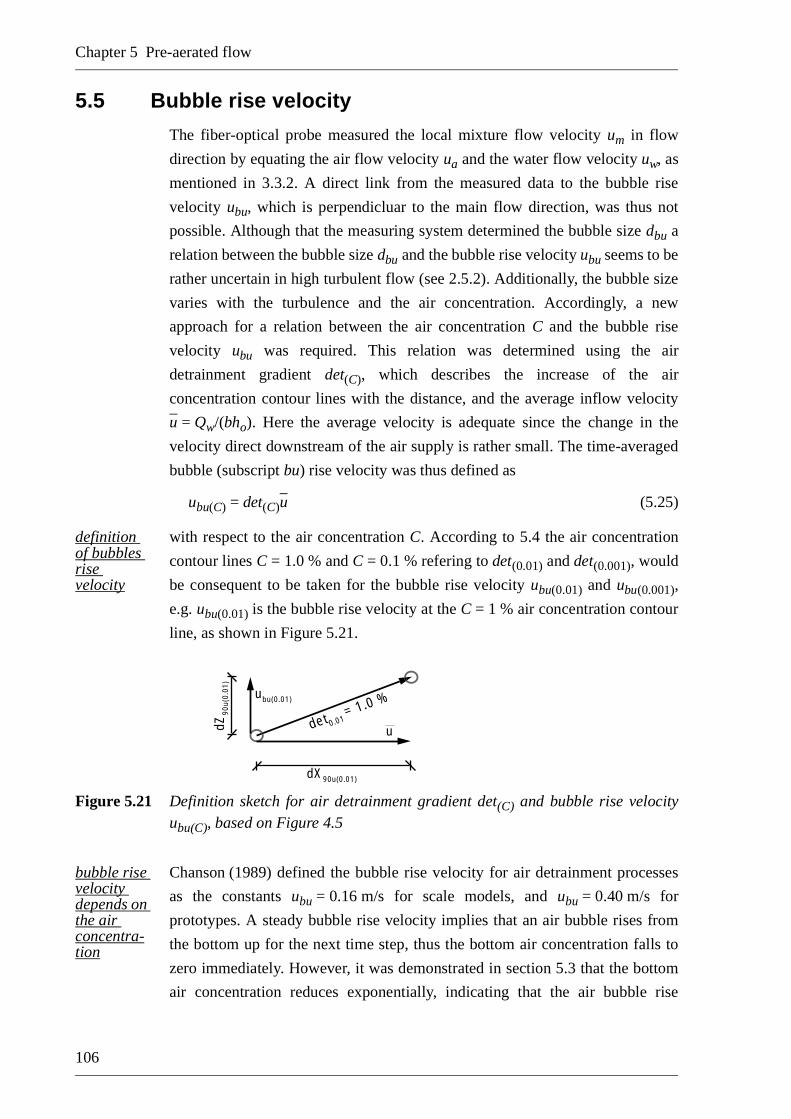
Chapter 5 Pre-aerated flow
106
5.5 Bubble rise velocity
The fiber-optical probe measured the local mixture flow velocity um in flow
direction by equating the air flow velocity ua and the water flow velocity uw, as
mentioned in 3.3.2. A direct link from the measured data to the bubble rise
velocity ubu, which is perpendicluar to the main flow direction, was thus not
possible. Although that the measuring system determined the bubble size dbu a
relation between the bubble size dbu and the bubble rise velocity ubu seems to be
rather uncertain in high turbulent flow (see 2.5.2). Additionally, the bubble size
varies with the turbulence and the air concentration. Accordingly, a new
approach for a relation between the air concentration C and the bubble rise
velocity ubu was required. This relation was determined using the air
detrainment gradient det(C), which describes the increase of the air
concentration contour lines with the distance, and the average inflow velocity
u = Qw/(bho). Here the average velocity is adequate since the change in the
velocity direct downstream of the air supply is rather small. The time-averaged
bubble (subscript bu) rise velocity was thus defined as
ubu(C) = det(C)u (5.25)
definition of bubbles rise velocity
with respect to the air concentration C. According to 5.4 the air concentration
contour lines C = 1.0 % and C = 0.1 % refering to det(0.01) and det(0.001), would
be consequent to be taken for the bubble rise velocity ubu(0.01) and ubu(0.001),
e.g. ubu(0.01) is the bubble rise velocity at the C = 1 % air concentration contour
line, as shown in Figure 5.21.
Figure 5.21 Definition sketch for air detrainment gradient det(C) and bubble rise velocityubu(C), based on Figure 4.5
bubble rise velocity depends on the air concentra-tion
Chanson (1989) defined the bubble rise velocity for air detrainment processes
as the constants ubu = 0.16 m/s for scale models, and ubu = 0.40 m/s for
prototypes. A steady bubble rise velocity implies that an air bubble rises from
the bottom up for the next time step, thus the bottom air concentration falls to
zero immediately. However, it was demonstrated in section 5.3 that the bottom
air concentration reduces exponentially, indicating that the air bubble rise
det 0.01 = 1.0 %
dX90u(0.01)
dZ90
u(0.
01)
ubu(0.01)
u

Development of Aerated Chute Flow
107
velocity depends on the local air concentration, in contrast to a linear
detrainment approach. Figure 5.18 shows that air concentration contours related
to small air concentrations decay slower than those connected to larger air
concentrations. This can be explained by: (1) Small air concentration contours
refer to small air bubbles whose rise velocity is reduced according to Figure 2.9,
or (2) Turbulent and diffusive effects act as a random generator and distribute
air bubbles in regions with smaller air concentration. This section aims to
present bubble rise velocities depending on the air concentration using equation
(5.25).
Figure 5.22 shows non-dimensional bubble rise velocities
(5.26)
non-dimens. bubble rise velocity depends on the streamwise Froude number
related to a concentration of C = 1 % as a function of the streamwise Froude
number Fo-min according to equation (5.11). The measurements refer to the four
investigated chute slopes So = 0 %, 10 %, 30 % and 50 %. Although the scatter
of data in Figure 5.22 a reduction of Ubu with Fo-min is noted. The data in the
brackets (♦) in Figure 5.22b and d result from small inflow Froude numbers
Fo ≤ 4 and are thus excluded from the analysis. Furthermore, the bubble rise
velocity falls to zero for Fo-min ≥ 13.8, indicating that air bubbles associated
with C = 1 % were kept at the chute bottom for large streamwise Froude
numbers. The slope of the function can be described as (Figure 5.22)
(5.27)
where F0 is the Froude number where Ubu = 0. The slope of the trend line
t = 0.029 is constant in Figure 5.22 and Figure 5.23. The constant F0 depends on
the relating air concentration contour line C in the same two figures (Table 5.4).
Equation (5.27) must be limited to Fo-min ≥ 7.5 and to Ubu ≤ 0.15 for C = 1.0 %
and to Ubu ≤ 0.10 for C = 0.1 % because these were the highest
non-dimensional bubble rise velocities observed.
Ubu
ubu C( )
gho
--------------=
Ubu t– Fo min– F0–( )= Fo min– 7.5≥

Chapter 5 Pre-aerated flow
108
a) b)
d) d)
Figure 5.22 Non-dimensional bubble rise velocity Ubu (5.26) for C = 1 % as a function ofstreamwise Froude number Fo-min according to (5.11), (–––) trend line witht = 0.029 (5.27) for a) So = 0 %, b) So = 10 %, c) So = 30 %, and d) So = 50 %,
region of data scatter
the streamwise Froude number Fo-min tends to overesti-mate Fo
From a physical point of view, the non-dimensional bubble rise velocity reduces
for steeper chute slopes due to the increasing turbulence. It would therefore be
evident if the slopes t of the trend lines in Figure 5.22 would increase for steeper
chute slopes. They are constant instead because the streamwise Froude number
Fo-min includes the chute slope already. The parameter Fo-min accounts in a
simple way for the cross flow features with a reducing flow depth h(x). It must
be emphasised that this analysis is based on a simply approach to describe the
bubble rise velocity in turbulent flow. The significant data scatter in Figure 5.22
allow only a qualitative description of the non-dimensional bubble rise velocity
Ubu
8 124
0.05
0.10
Fo-min
0
0.15
F0
Ubu
8 124
0.05
0.10
Fo-min
0
0.15
( )
F0
Ubu
8 124
0.05
0.10
Fo-min
0
0.15
F0
Ubu
8 124
0.05
0.10
Fo-min
0
0.15
( )
F0

Development of Aerated Chute Flow
109
which is approached by equation (5.27). However, this is the first attempt to
describe the behaviour of single bubble under such conditions and might be
improved in future.
bubble rise velocity related to C = 0.1 %
Figure 5.23 shows the same measurement as Figure 5.22 but refers to the
C = 0.1 % air concentration. A similar trend of the non-dimensional bubble rise
velocity Ubu can be noted except that the trend lines intersect the x-axis at
F0 = 10.5; the bubble rise velocity is thus zero for a higher streamwise Froude
number. The constant slope t of the trend line was again determined to t = 0.029.
The data point in brackets (Figure 5.23b) refers to a small inflow Froude
number and is therefore also excluded from the data analysis.
a) b)
c) d)
Figure 5.23 Non-dimensional bubble rise velocity Ubu (5.26) for C = 0.1 % as a function ofstreamwise Froude number Fo-min (5.11), (–––) trend line with t = 0.029 inequation (5.27) for a) So = 0 %, b) So = 10 %, c) So = 30 %, and d) So = 50 %,
region of data scatter
Ubu
8 124
0.05
0.10
Fo-min
0
0.15
F0
Ubu
8 124
0.05
0.10
Fo-min
0
0.15
( )
F0
Ubu
8 124
0.05
0.10
Fo-min
0
0.15
F0
Ubu
8 124
0.05
0.10
Fo-min
0
0.15
F0

Chapter 5 Pre-aerated flow
110
Table 5.4 Constants t and F0 for the bubble rise velocity refering to the air concentration
contour lines C from Figure 5.22 and Figure 5.23 in equation (5.27)
Example 5.7Problem: Find the bubble rise velocity ubu for a chute model of slope So = 30 %, water discharge
Qw = 198 l/s, inflow depth ho = 0.08 m, and flow depth at the point of inceptionh(Cmin) = 0.05 m.
Solution: With Fo = 0.198/(9.81•0.52•0.0083)0.5 = 5.59 and F(Cmin) = 0.198/(9.81•0.52•0.0053)0.5 = 11.31 from equation (3.1), the streamwise Froude number isFo-min = (5.59 + 11.31)/2 = 8.45 using equation (5.11). From equation (5.27), thenon-dimensional bubble rise velocity can be calculated to Ubu = –0.029(8.45 –13.8) = 0.155 for C = 1 % and Ubu = –0.029(8.45 – 11.5) = 0.088 for C = 0.1 %using the corresponding constants of Table 5.4.
Answer: The dimensional bubble rise velocity is ubu = 0.11•(9.81•0.08)0.5 = 0.014 m/s forC = 1 % and ubu = 0.06•(9.81•0.08)0.5 = 0.078 m/s for C = 0.1 % according to equation(5.26). Note the data scatter for this approach, thus this result claims only to be aqualitatively.
Figure 5.24 a) Trend line from Figure 5.22 and Figure 5.23 following equation (5.27), for (–––) C = 1.0 % and (---) C = 0.1 %
to find a bubble rise velocity for prototypes is rather uncertain
The non-dimensional bubbble rise velocity Ubu depends exclusively on the
streamwise Froude number Fo-min. Figure 5.25 shows a summary of all
dimensional bubble rise velocities ubu in [m/s] according to equation (5.25) for
all investigated chute slopes against the inflow Froude number Fo. This figure
aims to show the range of ubu observed in this project. Typically, one notes
0.02 ≤ ubu ≤ 0.12 m/s in Figure 5.25a, and for 0.0 ≤ ubu ≤ 0.08 m/s in Figure
t F0 max. scatter± Fo-min
C = 1.0 % 0.029 13.7 2.5
C = 0.1 % 0.029 11.8 2.0
Ubu-o
8 124
0.05
0.10
Fo-min
0
0.15

Development of Aerated Chute Flow
111
5.25b. This observation suggests that a bubble rise velocity under such flow
conditions in a Froude model is in the order of ubu ≈ 0.08 m/s for the
investigated air concentrations.
a) b)
Figure 5.25 Dimensional bubble rise velocity ubu [m/s] against inflow air concentration Fo a) C = 1.0 %, and b) C = 0.1 %
ubu [m/s]
105
0.05
0.10
Fo0
0.15ubu [m/s]
105
0.05
0.10
Fo0
0.15

Chapter 5 Pre-aerated flow
112

Development of Aerated Chute Flow
113
CHAPTER 6 AERATOR FLOW
6.1 Introduction
This chapter aims to present data of air concentration contours downstream of an aerator in
high-speed chute flows. The measurements were conducted similarly to the pre-aerated data
presented in Chapter 5 but the air was added by a 1:10 chute aerator of height tr = 15 mm, and
length lr = 150 mm. The air discharge Qa was supplied from the compressed air system
mentioned in the previous chapter. The aerator was located 2.0 m downstream of the jetbox to
obtain a hydraulically well defined upstream flow, as described in 3.2.2. In principle the same
experiments were conducted as for the pre-aerated flow, with the differences between the
streamwise air concentration development for both aeration systems being outlined in this
chapter. Although the flow features resulting from an air supply system were not the primary
objective of the present project, the detrainment process along a chute depends on the aeration
system and cannot be neglected, therefore.
6.2 Average air concentration
6.2.1 Aerator flow
air concentra-tion develop-ment
The principle development of air concentration profiles for aerator flow is, as
expected, similar to the pre-aerated measurements shown in 5.2.1. The average
air concentration C90 is the integral between the chute bottom and the mixture
flow depth h90 where the air concentration is C = 90 %, defined by equation
(4.3). The typical behaviour of the average air concentration is shown Figure
5.1, it was classified in: (1) Inflow air concentration Co, (2) Air detrainment
region C90,det between Co, and (3) Minimum air concentration C90,min, (4) Air
entrainment region C90,ent between C90,min, and (5) Uniform air concentration
C90u. Figure 6.1 shows an aerator and the downstream flow region. The air is
entrained from: (1) The bottom cavity due to the jet deflection, (2) The free
surface in the centre region by turbulence effects.

Chapter 6 Aerator flow
114
a) b)
Figure 6.1 Aerator and downstream flow region a) streamwise view, b) top view
jet trajectory
The region between the lower jet nappe and the chute bottom directly
downstream of the aerator is called the air cavity, with an air concentration
C = 100 %. The free surface air entrainment direct at the aerator must be
considered with special attention. The pressure field changes from a reasonable
hydrostatic profile phyd upstream of the aerator to negative pressure p < 0 in the
cavity immediately downstream of the deflector before it impinges with a high
bottom pressure p > phyd at the point of inception. This highly non-hydrostatic
pressure field causes turbulence which leads to an air entrainment from both,
the cavity and the free surface, direct at the aerator. This behaviour is
qualitatively shown in Figure 6.2. The air entrainment in this region is highly
developing and therefore not considered for the present data analysis.
a) b)
Figure 6.2 Qualitative pressure field at an aerator
u
phyd
p < 0
p > phyd
aerator
cavity
point ofimpact
recirculationzone
free surface aeration
pA

Development of Aerated Chute Flow
115
The data analysis starts at the point of jet impact, where the lower jet
trajectory impinges the chute bottom. This point collapses with the point of
maximum average air concentration Cmax. The jet trajectory length depends on
the spillway slope α, the ramp (deflector) angle θ, the pressure gradient ∆p
between the cavity pressure and the atmospheric pressure, and the upstream
Froude number Fo (Rutschmann and Hager 1990).
6.2.2 Effect of Froude number on air detrainment
average air concentra-tion curves
The effect of Froude number was analysed in Chapter 5 for pre-aerated flow
using average air concentration curves C90 for varying chute slopes So, constant
inflow depth ho and constant inflow air concentration β. Figure 6.3 shows the
streamwise average air concentration curves C90 for aerator flow as a function
of non-dimensional location X90u for the four bottom slopes So = 0 %, 10 %,
30 % and 50 %. More scatter are notable for aerator than for pre-aerated flow,
both at the inflow and the minimum air concentration regions, compared to
Figure 5.2. The uniform air concentration C90u for the aerator measurements in
Figure 6.3 seems to be roughly the same as for pre-aeration, details for the air
entrainment and uniform region are addressed in 6.2.8. The inflow air
concentration Co is more spread and larger for aerator than for pre-aerated flow
because the aerator produces significant spray, especially for high Froude
numbers.
a) b)
0.1
0 100 200
0.2
0.4
C90u = 0.10
Cmin
C90
Fo
Co
X90u
6.008.0010.0011.65
0.3
0 100 200
0.2
0.4
Cmin
C90 Fo
Co
X90u
4.006.008.009.7410.00
0.1
C90u = 0.14
0.3

Chapter 6 Aerator flow
116
c) d)
Figure 6.3 Average air concentration C90 for aerator flow as a function of non-dimensional distance X90u for various slopes, runs as in Figure 5.2, (---)uniform air concentration C90u, for a) So = 0 %, b) So = 10 %, c) So = 30 %,and d) So = 50 %
6.2.3 Air detrainment region
average air concentra-tion follows the same equation for aerator flow
The average air detrainment C90,det = a•X90u + Co for pre-aerated flow was
described by equation (5.2). The variable a describes the slope of the reducing
average air concentration with the distance varied between –0.003 ≤ a ≤ –
0.0017 for pre-aeration, depending on the chute slope So. Figure 6.4 shows the
same data as in Figure 5.3 for aerator flow. The air detrainment for aerator flow
(–––) follows the same linear trend as for pre-aerated (---) flow conditions. Note
the difference in the slope of the trend lines between the two air supply systems.
The average air concentration downstream of the aerator decreases faster for
aerator flow than for pre-aeration. The slope a of the trend line for aerator flow
was found to be a = –0.009 for So = 0 %, a = –0.0075 for So = 10 %, a = –
0.0065 for So = 30 % and a = –0.0050 for So = 50 %.
more air is detrained for aerator flow
The larger air detrainment downstream of an aerator for small bottom slope
can be explained by the non-hydrostatic pressure gradient in the impact zone
leading to a larger air detrainment (see 2.5.2). The air detrainment gradients
depend on the exact aerator geometry and the upstream flow conditions. The
aerator design needs more attention in future.
0 100 200
0.2
0.4
Cmin
C90
Fo
Co
X90u
4.006.008.009.4311.00
0.1
C90u = 0.20
0.3
4.00 0.0606.00 0.0608.00 0.0609.43 0.06011.00 0.050
0 100 200
0.2
0.4
Cmin
C90
Fo
Co
X90u
4.006.008.009.4311.00
0.1
C90u = 0.27
0.3

Development of Aerated Chute Flow
117
a) b)
c) d)
Figure 6.4 Average air detrainment C90,det as a function of non-dimensional distance X90u
for various chute slopes, data as in Figure 6.3, (–––) equation (5.2) for aeratorflow, (---) trend lines for pre-aerated measurements (Figure 5.3), for a)So = 0.0 %, a = –0.009, b) So = 10 %, a = –0.0075, c) So = 30 %, a = –0.0065 d) So = 50 %, a = –0.005
6.2.4 Effect of chute slope
Figure 6.5 shows thw parameters a for aerator flow as a function of the sine of
the chute angle α, with the best fit (R2 = 0.90)
. (6.1)
reduced pressure gradient in the point of impact for steep chutes
Also plotted is the corresponding curve according to equation (5.3) for
pre-aerated flow. Both equations (5.3) and (6.1) have the common point
a(α = 90°) = 0. Note the steeper gradient a for aerator flow which is almost
trippled for flat slopes, indicating that more air under otherwise identical
conditions is detrained for this flow condition. Figure 6.5 shows furthermore
6.00 0.0508.00 0.05010.00 0.05011.65 0.050
0 100 200
0.2
0.4
Cmin
C90,det
Fo
X90u
6.008.0010.0011.65
0 100 200
0.2
0.4
Cmin
C90,det
Fo
Co
X90u
4.006.008.009.7410.00
0 100 200
0.2
0.4
Cmin
C90,det
Fo
X90u
4.006.008.009.4311.00
4.00 0.0606.00 0.0608.09.0609.43 0.06011.00 0.050
0 100 200
0.2
0.4
Cmin
C90,det
Fo
X90u
4.006.008.009.4311.00
a 0.0085 α 1–sin( )=

Chapter 6 Aerator flow
118
that the two lines are getting closer for steep chute angles α because the
pressure gradient in the point of jet impact for aerator flow reduces for steeper
chute slopes with the sine of chute angle.
Inserting equation (6.1) in equation (5.2) allows to present a general relation
for air detrainment for aerator flow
, (6.2)
with Co as the average inflow air concentration, and Cmin as the average
minimum air concentration from equation (5.12).
Figure 6.5 Parameter a from equation (6.1) as a function of the sine of the chute angle sinαfor
(––) aerator flow, R2 = 0.90, and (---) pre-aerated flow by equation (5.3)
6.2.5 Air detrainment per chute distance
The interest to determine the average air detrainment per chute distance
∆C90,det/∆x for practical application was outlined in 5.2.4. Following that
procedure, equation (6.2) can be written as
, (6.3)
C90 det, 0.0085 α 1–sin( )X90u Co+= Co C90det Cmin≥ ≥
0
sinα0.2 0.4 0.6 0.8
0
-0.005
-0.010
a
∆C90 det,∆x
---------------------0.0085 α 1–sin( )
h90u-----------------------------------------= Co C90 det, Cmin≥ ≥

Development of Aerated Chute Flow
119
and in terms of specific discharge qw = Qw/b and surface roughness kst as
(6.4)
with the corresponding minimum at sinα = 3/13. Figure 6.6 shows air
detrainment per chute meter for aerator flow (–––) and pre-aerated flow (---),
with a maximum of
. (6.5)
Figure 6.6 Air detrainment ∆C90,det per chute meter ∆x = 1 m as a function of the sine ofchute angel α, for aerator flow (–––) equation (6.4), and pre-aerated flow (---)equation (5.8)
Example 6.1
Problem: Consider the same spillway as in Example 5.1 and Example 5.2 again. Assume anaerator dimensionally similar to the deflector used for the present chute model. Keepall other quantities identical i.e. kst = 90 m1/3/s, So = 10 %, 20 %, 30 %, 40 % and50 %, and 40 m2/s ≤ qw ≤ 140 m2/s. Compare a) air detrainment ∆C90,det per chutemeter ∆x = 1 m for aerator flow and pre-aerated flow conditions, and b) the maximumair detrainment rates with (∆C90,det/m)max = –0.0043(kst/qw)3/5 (equation (6.5)).
Solution: See Example 5.1 and Example 5.2Answer: See Table 6.1 and Table 6.2. Note that air detrainment is almost tripled for aerator as
compared to pre-aerated flow conditions.
∆C90 det,∆x
--------------------- 0.0085kst
qw------
35---
αsin( )310------
αsin 1–( )=
∆C90 det,∆x
---------------------
max0.00– 43
kst
qw------
35---
= 0.09 αsin 0.45≤ ≤
0
sinα0.2 0.4 0.6 0.8
0
-0.0015
-0.0030
-0.0045
∆C90,det
∆x(ks/qw)3/5

Chapter 6 Aerator flow
120
Table 6.1 Air detrainment ∆C90,det per meter chute length for pre-aeration compared to
aerator flow
Table 6.2 Maximum air detrainment per meter (∆C90,det/m)max depending on specific
discharge qw for pre-aeration, compared to aerator flow
6.2.6 Minimum air concentration
minimum air concentra-tion follows the same equation for aerator flow
The minimum air concentration Cmin is a function of the streamwise Froude
number Fo-min as described for pre-aerated flow in 5.2.6 by equation (5.12).
Figure 6.7 shows the minimum average air concentration Cmin against the
streamwise inflow Froude number Fo-min for all chute slopes So, for aerator
flow with the measurements limited to Fo ≥ 4. The best fit for the minimum
average air concentration for aerator flow was found to (R2 = 0.83)
. (6.6)
Although the average air concentration detrains much quicker for aerator flow
than for pre-aeration, the minimum air concentration seems similar to
pre-aerated flow conditions. This can be traced back to the fact that the
minimum average air concentration depends only on the air transport capacity
at the point of inception xi, and not on the air supply device. In other words, the
flow at xi has ´forgotten´ the air supply device.
So 10 % 20 % 30 % 40 % 50 %
h90u = hwu 1.79 m 1.45 m 1.29 m 1.18 m 1.10 m
Pre-aeration, ∆C90,det/m–0.151 %/
m–0.166 %/
m–0.166 %/
m–0.160 %/
m–0.150 %/
m
Aerator, ∆C90,det/m–0.438 %/
m–0.470 %/
m–0.471 %/
m–0.453 %/
m–0.426 %/
m
qw 40 m2/s 60 m2/s 80 m2/s 100 m2/s 120 m2/s 140 m2/s
Pre-aeration,(∆C90,det/
m)max
–0.244 %/m
–0.191 %/m
–0.161 %/m
–0.141 %/m
–0.126 %/m
–0.115 %/m
Aerator, (∆C90,det/
m)max
–0.699 %/m
–0.548 %/m
–0.461 %/m
–0.404 %/m
–0.362 %/m
–0.330 %/m
Cmin 0.015Fo m– i n=

Development of Aerated Chute Flow
121
Figure 6.7 Minimum air concentration Cmin against streamwise Froude number Fo-min foraerator flow for all chute slopes, Fo ≥ 4, (–––) equation (6.6), correlation
R2 = 0.83
6.2.7 Effect of inflow depth
the average air detrain-ment is also not influence by the inflow depth
It was demonstrated in 5.2.7 that the inflow depth ho has no influence on the air
detrainment process relating to the average air concentration C90,det. The
constant aerator ramp height tr = 15 mm affects the air detrainment process for
aerator flow as shown in 6.2.3. It may be assumed that one aerator geometry,
which varies relative to the flow depth h(x), changes the detrainment behaviour.
Figure 6.8 shows, as a typical example, the effect of the inflow depth ho on the
average air detrainment C90 for the chute slope So = 30 %. The figure shows
that all air concentrations C90 reduce similarly to the measurements shown in
Figure 6.4c, and a variable inflow depth between 0.05 m ≤ ho ≤ 0.11 m has no
effect on the detrainment gradient, therefore. Nevertheless that no affect was
found in this section, a influence from the uniform flow depth h90u to the air
detrainment gradient ∆C90,det/∆x was proved by equation (6.3). This can be
explained by the limitation range of the jetbox opening up to ho = 0.12 m and
the water discharge up to Qw = 250 l/s. Further investigations would be
desirable.
Fo ho SoCmin
10 200
0.1
0.2
0.3
Fo-min
6.00 0.05 0.008.00 0.05 0.0010.00 0.05 0.0011.65 0.05 0.0013.00 0.05 0.004.00 0.05 0.106.00 0.06 0.107.00 0.06 0.108.00 0.06 0.109.00 0.06 0.109.74 0.06 0.1010.00 0.05 0.104.00 0.06 0.306.00 0.06 0.308.00 0.06 0.309.43 0.06 0.3011.00 0.05 0.304.00 0.10 0.506.00 0.08 0.508.00 0.06 0.504.00 0.06 0.506.00 0.06 0.508.00 0.06 0.509.43 0.06 0.5011.00 0.05 0.50

Chapter 6 Aerator flow
122
Figure 6.8 Average air detrainment C90,det as a function of non-dimensional distance X90u
for various flow depths 0.05 m ≤ ho ≤ 0.11 m, for the chute slope So = 30 %,(–––) equation (5.2) a = –0.0065, (---) trend line for pre-aerated measurements(Figure 5.7)
6.2.8 Air entrainment region
the aerator effects the air concentra-tion contour lines in the near flow field
The streamwise average air entrainment concentration C90,ent downstream of
the point of inception xi was considered in 5.2.9 for pre-aerated flow. The point
of inception for the pre-aerated measurements and non-aerated deflector flow
was defined at the point where the average air concentration reached its
minimum at Cmin. For non-aerated jetbox flow measurements, the air
entrainment started at the jetbox. Figure 6.9a shows the effect of free surface
aeration by means of air concentration contour lines for non-aerated jetbox flow
and for deflector flow, both with and without upstream air supply. Whereas air
concentrations increase almost linearly in this typical fan-shaped behaviour
with origin at the point of inception for jetbox flow as in Figure 5.9 (---), a chute
deflector entrains air locally and thus increases significantly the air
concentration shortly downstream from the deflector between 0 ≤ X90u ≤ 100
(––––). Further downstream, an air entrainment pattern similar to the jetbox
flow develops. Note the almost identical contour gradients of the two respective
air supply systems at the downstream end of Figure 6.9a. They are in
agreement, except for the C = 99 % contour line, which may be due to the
generation of shock waves along the chute and their influence on the flow close
to the free surface. Accordingly the effect of the aerator is large in its near flow
field, but appears to have practically no effect on the far flow field. Otherwise
expressed, chute flow far away from an air supply device has forgotten its
history, and only local effects are retained (Kramer et al. 2003).
0 100 200
0.2
0.4
Cmin
C90,det
X90u
3.00 0.1104.00 0.1006.00 0.0808.00 0.0659.04 0.06011.00 0.050
Fo ho

Development of Aerated Chute Flow
123
average air concentra-tion comparing pre-aerated and non-aerated flow
The average cross-sectional air concentration development C90 as a function
of relative distance X90u is shown in Figure 6.9b for pre-aerated jetbox flow
with β = 21 %, non-aerated jetbox flow with β = 0 %, pre-aerated aerator
flow with β = 21 %, and non-aerated deflector flow with β = 0 %. For non-
aerated jetbox flow , C90 increases almost linearly with distance, in contrast
to non-aerated deflector flow involving a local maximum beyond the chute
deflector, then drops and practically runs parallel to curve for larger
distances. The pre-aerated jetbox flow differs only in the detrainment region
from pre-aerated deflector flow , as outlined in 6.2.3. Downstream of the
point of inception at xi = 100 all curves run parallel up to uniform average air
concentration C90u = 0.24 at X90u = 230.
a) b)
Figure 6.9 a) Contour plot for non-aerated flow Fo = 6.0, So = 50 %, shock wave, for (–––) non-aerated deflector flow, (---) non-aerated jetbox flow. Runs as inFigure 5.9; b) Average air concentration C90 as a function of non-dimensionaldistance X90u, for pre-aerated jetbox flow with β = 21 %, non-aerated jetboxflow with β = 0 %, pre-aerated deflector flow with β = 21 %, andnon-aerated deflector flow with β = 0 %, respectively. (-.-.-) uniform airconcentration C90u
air entrain-ment function for aerator flow
Figure 6.9b shows that each air supply device has its particular features
resulting in a specific near-field flow pattern. The turbulence level of chute
flows is relatively high, thus local characteristics are diffused beyond
X90u ≈ 100. The air-water mixture flow features of the far-field depend
exclusively on the chute characteristics. For a prismatic rectangular chute, these
are boundary roughness and chute slope. For both jetbox and deflector flows,
the local entrainment effect has to be separated from the far-flow field,
therefore.
0 100 200
0.5
1
1.5
Z90u
X90u
free surface aeration
point ofinception
0.99
0.950.9
0.5
0.10.05
0.01
0.001
0.01
0.001
0.5
0.95
C90u
X90u0 100 200
0.2
0.4C90
Cmin
Co
1
24
3
point ofinception

Chapter 6 Aerator flow
124
near and far flow field
It was stipulated that average air concentration in the far field does
continuously increase, from a boundary value to equilibrium, as proposed in
5.2.9. This trend was checked for jetbox flow, with Figure 6.10 showing data for
aerator flow shifted on C90,ent = C90utanh(d•X90u) as described by equation
(5.13). The variable d in the tangent hyperbolic function describes the curve
slope in the origin. For jetbox flow conditions two different variables were
found to describe the air entrainment, depending on the air supply. For
non-aerated jetbox flow the air entrainment from the free surface was found to
follow the above mentioned equation with d = 0.006 whereas for pre-aerated
jetbox flow d = 0.004. Deflector flow conditions showed a different behaviour,
both variables were found to be d = 0.004 independent of the air supply. This
can be explained with the above mentioned approach. The deflector acts like a
turbulence generator which entrains, in fact, air locally to a certain amount, but
the far flow field is not influenced. The transition zone between the local
deflector region and the uniform region is similar to conditions where air was
supplied to the inflow, whereas the initial air entrainment was nonexistent for
non-aerated jetbox flow. Two feats are notable in Figure 6.10 (c and d), relating
to the data sets with the smallest upstream Froude numbers Fo and thus the
smallest discharges. Both data sets appear to deviate at their end reaches from
the general trend. It is therefore presumed that scale effects and minute shock
waves have effected these data points, but that the general trend is not
influenced, as discussed in 5.2.9.
a) b)
4.006.006.007.008.008.008.009.009.74
X90u
Cmin
C90u
(10%)=0.15
0 200 400
0.2
0.4C90,ent
Fo
X90u
Cmin
C90u
(30%)=0.23
0 200 400
0.2
0.4C90,ent
Fo3.004.004.006.006.008.008.009.4311.00

Development of Aerated Chute Flow
125
c) d)
Figure 6.10 (–––) Average air entrainment C90,ent according to equation (5.13) as afunction of non-dimensional distance X90u for aerator flow, and a) So = 10 %,b) So = 30 %, c) So = 50 %, and d) non-aerated deflector flow, So = 50 %. Withthe uniform air concentration a) C90u = 0.15 (pre-aerated flow C90u = 0.20),b) C90u = 0.23, c) C90u = 0.29, and d) non-aerated deflector flow C90u = 0.29
uniform air concentra-tion
The uniform air concentration C90u shown in Figure 6.10 for aerator flow is
identical to the pre-aerated measurements shown in Figure 5.10, except for the
measurements on the flattest chute So = 10 %. This bottom slope is too flat to
produce sufficient turbulence to entrain significant amounts of air. Figure 6.10a
shows that air is entrained downstream of the point of inception at Xi = 200 up
to C90u = 0.15, whereas air was entrained up to C90u = 0.20 for pre-aerated flow
in Figure 5.10a at Xi = 270. The uniform air concentration is thus between
0.15 ≤ C90u(10 %) ≤ 0.20 for So = 10 %. However, the overall trend is not
effected from this slight deviation, and equations C90u = 0.33(sinα)0.25 (5.14),
and C90,ent = 0.33(sinα)0.25tanh(d•X90u) (5.15) are also valid for chute aerators.
6.3 Bottom air concentration
6.3.1 Effect of Froude number
the bottom air detrains exponen-tially, down-stream of the cavity
The bottom air concentration Cb gives the most meaningful information about
the potential of chute cavitation protection. Figure 6.11 shows streamwise
bottom air concentration curves Cb for aerator flow as a function of X90u in a
semi-logarithmic plot, similarly to the pre-aerated flow measurements shown in
Figure 5.12. The bottom air concentration for the two air supply systems vary
mainly in the near flow field close to the aerator. The bottom air concentration
X90u
Cmin
C90u
(50%)=0.29
0 200 400
0.2
0.4C90,ent
Fo4.004.006.006.008.008.009.4311.00
scale effect
X90u
Cmin
C90u
(50%)=0.29
0 200 400
0.2
0.4C90,ent
Fo
scale effect
3.004.004.006.006.008.008.009.3811.00

Chapter 6 Aerator flow
126
in the cavity immediately downstream of the aerator is Cbo = 100 % at X90u ≤ 5,
whereas a characteristic value of Cbo ≈ 5 % was observed for jetbox flow at
X90u ≈ 0 (Figure 5.12).
a) b)
c) d)
Figure 6.11 Bottom air concentration Cb for aerator flow as a function of non-dimensionaldistance X90u for various slopes a) So = 0 %, b) So = 10 %, c) So = 30 %, andd) So = 50 %
four instead of three regions as for pre- aeration
The data for pre-aerated flow were classified into three regions, namely: (1) Air
detrainment region, (2) Minimum air region, and (3) Increasing air
concentration region. Figure 6.11 shows that region (1) must be split into two
portions for aerator flow: (1.1) A region with a large detrainment which is
directly influenced by the aerator, and (1.2) A transition zone downstream of the
kink in the detrainment curve where exponential detrainment establishes,
similar to observations for pre-aeration. Accordingly, four flow zones were
defined for aerator flow. Yet, the flow zone directly influenced by the aerator
was not subject of this project. The detrainment zone (1.2) not directly
X90u100 200
Cb Fo6.008.0010.0011.65
Cb = 1 %
10-4
10-3
10-2
10-1
1
X90u100 200
Cb
Cb = 1 %
10-4
10-3
10-2
10-1
14.006.008.008.0010.00
Fo
X90u100 200
CbFo
Cb = 1 %
10-4
10-3
10-2
10-1
14.006.008.009.4311.00
X90u100 200
Cb
Cb = 1 %
10-4
10-3
10-2
10-1
1Fo 4.00
6.008.009.4311.00

Development of Aerated Chute Flow
127
influenced by the deflector shows a similar fan-shaped behaviour as pre-aerated
flow for the streamwise development of the bottom air concentration in a
semi-logarithmic plot. It can also be observed that the inflow Froude number Fo
determines the detrainment slope.
6.3.2 Air detrainment region
steeper bottom air detrain-ment gradients for aerator flow
Figure 6.12 shows the corresponding data as Figure 6.11 for the bottom air
detrainment portion. The bottom air detrainment in the semi-logarithmic plot
follows Cb,det = Cboe-mX90u as in equation (5.16). The variable m is the slope of
the trend lines, it depends on the inflow Froude number Fo and the inflow
bottom air concentration Cbo determined at the kink of the detrainment lines,
downstream of region (1.1) influenced by the deflector. The detrainment region
for aerator flow was thus defined between Cbo and the minimum air
concentration Cb,min.
higher bottom air detrain-ment for small slopes
The bottom air detrainment slope m for pre-aerated flow was demonstrated
to be m= nFo–2.50 according to equation (5.17). Figure 6.12 shows that the
bottom air detrainment slope for aerator flow depends also on the inflow Froude
number Fo. Therefore equation (5.17) for aerator flow was applied, using the
variable n to account for chute slope. Figure 6.13 shows the variable m as a
function of the inflow Froude number Fo for the four investigated chute slopes
for aerator flow, in comparison to pre-aerated flow. Smaller deviations for the
chute slopes So = 0 % and 10 % were observed, whereas the slope m differ to
pre-aerated measurements for So = 30 % and 50 %. The deviations can be
explained by higher pressure gradients in the impact zone for flat chute slopes.
Therefore, the variable n in equation (5.17) depends exclusively on the chute
slope, ranging between 2.22 ≤ n ≤ 30.30 for aerator flow.
a) b)0 5 10
0.2
0.4
Fo
mm = 30.30Fo
-2.50
m = 14.42Fo
-2.50
0 5 10
0.2
0.4
Fo
mm = 18.80Fo
-2.50
m = 9.88Fo
-2.50
X90u100 200
Cb,det
Cb = 1 %
10-4
10-3
10-2
10-1
1 Fo m6.00, 0.3908.00, 0.11010.00, 0.05111.65, 0.037
m
X90u100 200
Cb,det
Cb = 1 %
10-4
10-3
10-2
10-1
1 Fo m4.00, 0.5746.00, 0.2318.00, 0.15210.65, 0.035

Chapter 6 Aerator flow
128
c) d)
Figure 6.12 Bottom air concentration in the detrainment region Cb,det as a function of non-dimensional distance X90u for various bottom slopes a) So = 0 %, b) So = 10 %,c) So = 30 %, and d) So = 50 %, (–––) equation (5.16), (-·-·-) kink-linedownstream of region (1.1) directly influenced by the aerator
a) b)
0 5 10
0.2
0.4
Fo
mm = 2.54Fo
-2.50
m = 8.79Fo
-2.50
0 5 10
0.2
0.4
Fo
mm = 2.22Fo
-2.50
m = 7.18Fo
-2.50
X90u100 200
Cb,det
Cb = 1 %
10-4
10-3
10-2
10-1
1
6.00, 0.0478.00, 0.0249.43, 0.019
Fo m4.00, 0.069
11.00, 0.015
X90u100 200
Cb,det
Cb = 1 %
10-4
10-3
10-2
10-1
1
6.00, 0.0318.00, 0.0249.43, 0.017
Fo m4.00, 0.064
11.00, 0.014
0 5 10
0.2
0.4
Fo
mm = 30.30Fo
-2.50
m = 14.42Fo
-2.50
0 5 10
0.2
0.4
Fo
mm = 18.80Fo
-2.50
m = 9.88Fo
-2.50

Development of Aerated Chute Flow
129
c) d)
Figure 6.13 Bottom air detrainment gradient m as a function of inflow Froude number Fo
for a) So = 0 %, n = 30.30, R2 = 0.89, b) So = 10 %, n = 18.80, R2 = 0.97,
c) So = 30 %, n = 2.54, R2 = 0.66, and d) So = 50 %, n = 2.22, R2 = 0.78,(–––)equation (5.17) for aerator flow and (---) pre-aerated flow from Figure 5.14
6.3.3 Effect of chute slope
bottom air detrain-ment for aerator flow
The effect of chute slope on the bottom air detrainment Cb,det for pre-aerated
flow was derived in 5.3.3 by equation (5.19) and Figure 5.15. Figure 6.14a
shows the same effect for aerator flow in relation to pre-aerated measurements.
All curves follow a power law as proposed by equation (5.17) with a variable n,
depending on the chute slope and the air supply system. A large detrainment
gradient for Froude numbers Fo ≤ 4 was found, whereas the bottom slope has no
major influence on the detrainment gradient for Fo ≥ 12. The variable n for
pre-aeration ranged between 7.18 ≤ n ≤ 14.42, the correlation between n and the
chute slope So was described by equation (5.18) (Figure 6.14b). The bottom air
detrainment parameter n for aerator flow had a wider range between
2.22 ≤ n ≤ 30.30 and can be described by (R2 = 0.89)
. (6.7)
0 5 10
0.2
0.4
Fo
mm = 2.54Fo
-2.50
m = 8.79Fo
-2.50
0 5 10
0.2
0.4
Fo
mm = 2.22Fo
-2.50
m = 7.18Fo
-2.50
n 30 0.006So⋅=

Chapter 6 Aerator flow
130
a) b)
Figure 6.14 a) Superposition of curves m as a function of inflow Froude number Fo fromFigure 6.13 for all bottom slopes, b) (–––) parameter n from Figure 6.13 as a
function of chute slope So, R2 = 0.89 for aerator flow equation (6.7), (---)equation (5.18) for pre-aerated flow
The general equation for the bottom air detrainment for aerator flow can be
described as
. (6.8)
no influence of the deflector for steeper chute slope
This section demonstrates that a deflector influences the behaviour of the air in
the near flow field downstream of the air supply such that the bottom air
detrainment for smaller chute slopes So is the multiple of that for pre-aerated
flow. For chute slopes So ≥ 30 % the deflector has a small influence to Cb,det,
however. This again can be explained by a higher pressure peaks in the impact
zone for flat chute slopes, which presses the air away from the bottom.
6.3.4 Minimum bottom air concentration
minimum bottom air concentra-tion is similar to pre-aeration
The minimum bottom air concentration Cb,min for pre-aerated flow was
described in 5.3.4. Figure 6.15 shows the minimum bottom air concentration
Cb,min as a function of streamwise Froude number Fo-min = (Fo+ F(Cb,min))/2
according to equation (5.11) for aerator flow. The same trend as for pre-aerated
flow results in
. (6.9)
So = 10 %
So = 50 %
So = 30 %
So = 10 %
So = 0 %
So = 50 %
So = 30 %
So = 0 %
0 5 10
0.2
0.4
Fo
m
m = nFo
-2.50
aerator
pre- aeration
0
n = 30•0.006So
So0.4 0.8
30 n
15
n = 7.2•0.006So + 6.6
Cb det, Cboe30 0.006
So⋅– Fo2.50– X90u= Cb min, Cb det, Cbo≤ ≤
Cb min, 3.6 107–⋅ e
0.78Fo m– i n=
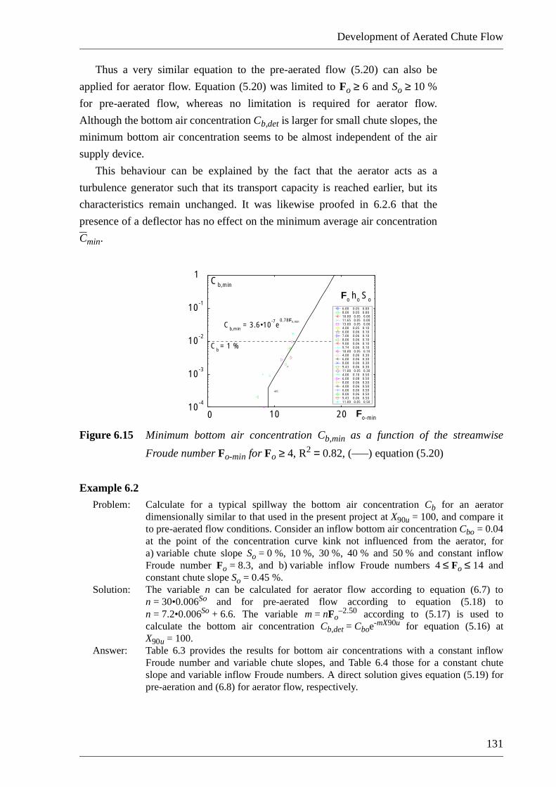
Development of Aerated Chute Flow
131
Thus a very similar equation to the pre-aerated flow (5.20) can also be
applied for aerator flow. Equation (5.20) was limited to Fo ≥ 6 and So ≥ 10 %
for pre-aerated flow, whereas no limitation is required for aerator flow.
Although the bottom air concentration Cb,det is larger for small chute slopes, the
minimum bottom air concentration seems to be almost independent of the air
supply device.
This behaviour can be explained by the fact that the aerator acts as a
turbulence generator such that its transport capacity is reached earlier, but its
characteristics remain unchanged. It was likewise proofed in 6.2.6 that the
presence of a deflector has no effect on the minimum average air concentration
Cmin.
Figure 6.15 Minimum bottom air concentration Cb,min as a function of the streamwise
Froude number Fo-min for Fo ≥ 4, R2 = 0.82, (–––) equation (5.20)
Example 6.2
Problem: Calculate for a typical spillway the bottom air concentration Cb for an aeratordimensionally similar to that used in the present project at X90u = 100, and compare itto pre-aerated flow conditions. Consider an inflow bottom air concentration Cbo = 0.04at the point of the concentration curve kink not influenced from the aerator, fora) variable chute slope So = 0 %, 10 %, 30 %, 40 % and 50 % and constant inflowFroude number Fo = 8.3, and b) variable inflow Froude numbers 4 ≤ Fo ≤ 14 andconstant chute slope So = 0.45 %.
Solution: The variable n can be calculated for aerator flow according to equation (6.7) ton = 30•0.006So and for pre-aerated flow according to equation (5.18) ton = 7.2•0.006So + 6.6. The variable m= nFo
–2.50 according to (5.17) is used tocalculate the bottom air concentration Cb,det = Cboe
-mX90u for equation (5.16) atX90u = 100.
Answer: Table 6.3 provides the results for bottom air concentrations with a constant inflowFroude number and variable chute slopes, and Table 6.4 those for a constant chuteslope and variable inflow Froude numbers. A direct solution gives equation (5.19) forpre-aeration and (6.8) for aerator flow, respectively.
6.00 0.05 0.00
8.00 0.05 0.0010.00 0.05 0.0011.65 0.05 0.0013.00 0.05 0.004.00 0.05 0.106.00 0.06 0.107.00 0.06 0.108.00 0.06 0.109.00 0.06 0.109.74 0.06 0.1010.00 0.05 0.104.00 0.06 0.306.00 0.06 0.308.00 0.06 0.309.43 0.06 0.3011.00 0.05 0.304.00 0.10 0.506.00 0.08 0.508.00 0.06 0.504.00 0.06 0.506.00 0.06 0.508.00 0.06 0.509.43 0.06 0.5011.00 0.05 0.50
Cb,min
Cb = 1 %
10-4
10-3
10-2
10-1
1
10 20
Fo ho So
Fo-min
Cb,min
= 3.6•10-7e
0.78Fo,min
0

Chapter 6 Aerator flow
132
Table 6.3 Bottom air concentration Cb in %, depending on the chute slope So for Fo = 8.3
and Cbo = 0.04, at X90u = 100 (Example 6.2a)
Table 6.4 Bottom air concentration Cb in %, depending on the inflow Froude number Fo
with So = 0.45, and Cbo = 0.04, at X90u = 100 (Example 6.2b)
6.4 Air detrainment gradient
6.4.1 Effect of Froude number
air detrain-ment gradients are steeper for aerator flow
The principle of the air detrainment gradient det(C) is defined by equation (4.5),
and a typical example is shown in Figure 4.5. The detrainment gradients for
pre-aeration are considered in 5.4. This section aims to compare these data to
aerator flow. A summary for all detrainment gradients det(C) and bubble rise
velocities ubu(C) = det(C)u as defined in (5.25), is given in Appendix E. Figure
6.16 is the equivalent to Figure 5.18 for pre-aerated flow, it shows air
detrainment gradients det(C) for aerator flow against the inflow Froude number
Fo for the four investigated chute slopes So = 0 %, 10 %, 30 % and 50 %,
referring to C = 5 %, 1 % and 0.1 %. The linear trend lines correlate with the
So 0 % 10 % 20 % 30 % 40 % 50 %
n, pre-aeration 13.80 10.91 9.19 8.15 7.53 7.16
n, aerator 30.00 17.99 10.78 6.46 3.88 2.23
m, pre-aeration 0.070 0.055 0.046 0.041 0.038 0.036
m, aerator 0.151 0.091 0.054 0.033 0.200 0.012
Cb(X90u = 100) in %, pre-aeration
0.003 0.016 0.040 0.066 0.089 0.110
Cb(X90u = 100) in %, aerator
0 0.001 0.018 0.154 0.567 1.240
Fo 4 6 8 10 12 14
n, pre-aeration 7.32 7.32 7.32 7.32 7.32 7.32
n, aerator 3.00 3.00 3.00 3.00 3.00 3.00
m, pre-aeration 0.228 0.083 0.040 0.023 0.014 0.010
m, aerator 0.094 0.034 0.017 0.090 0.060 0.040
Cb(X90u = 100) in %, pre-aeration
0 0.001 0.073 0.401 0.986 1.472
Cb(X90u = 100) in %, aerator
0 0.133 0.762 1.548 2.191 2.657

Development of Aerated Chute Flow
133
gradients det(0.05), det(0.01) and det(0.001). Again, the trend of det(0.05) is weak
and no defined trend was observed. Note that the scale of the vertical axis varies
between 0 ≤ det(C) ≤ 0.08 as compared to 0 ≤ det(C) ≤ 0.02 for pre-aerated flow
in Figure 5.18. This proofs that the overall detrainment gradient for aerator flow
is much larger than for pre-aerated flow.
the inflow Froude number and chute slope influence the detrain-ment gradient
It was demonstrated for the pre-aerated measurements that both, the inflow
Froude number Fo and the chute slope So influence the air detrainment gradients
det(0.01) and det(0.001). The air detrainment gradients det(0.01) and det(0.001) for
aerator flow show a similar behaviour, apart from the higher values.
Furthermore, Figure 6.16 shows that the trend lines for aerator flow run more
parallel as those for pre-aerated flow.
a) b)
c) d)
Figure 6.16 Air detrainment gradient det(C) for aerator flow as a function of inflow Froudenumber Fo with linear trend lines det(0.05) (–––), det(0.01) (---) and det(0.001) (-·-·-·) for a) So = 0.0 % b) So = 10 %, c) So = 30 %, and d) So = 50 %
det(C)
105
0.04
0.08
Fo
0
det(0.05)
det(0.01)
det(0.001)
det(C)
105
0.04
0.08
Fo
0
det(0.05)
det(0.01)
det(0.001)
det(C)
105
0.04
0.08
Fo
0
det(0.05)
det(0.01)
det(0.001)
det(C)
105
0.04
0.08
Fo
0
det(0.05)
det(0.01)
det(0.001)

Chapter 6 Aerator flow
134
6.4.2 Effect of chute slope
detrain-ment gradients are almost parallel
Figure 6.16 shows the air detrainment gradients det(C) for the four investigated
chute slopes for aerator flow. In Figure 6.17 the trend lines det(0.01) and
det(0.001) were superimposed (thick lines) as for pre-aeration from Figure 5.18
(thin lines). The trend lines for pre-aeration have a common point r, as specified
in Table 5.3, depending on the air concentration C, and a variable slope
depending on the chute slope So, whereas the trend lines for aerator flow are
almost parallel. The largest detrainment gradients result for the chute slope
So = 0 % for both det(0.01) and det(0.001), respectively. For chute slopes So > 0 %
the trend lines are lower indicating smaller air detrainment for a given inflow
Froude number. The air detrainment gradient for aerator flow can be described
as
(6.10)
with a = f(C) describing the slope of the trend lines and b depending on the
chute slope. The constant a is the average of the fairly parallel trends line for
aerator flow shown in Figure 6.17 and b is the intersection at Fo = 0 (Table 6.5).
a) b)
Figure 6.17 Air detrainment gradients det(C) as a function of Froude number Fo asdescribed by equation (6.10) for So = 0.0 % (–––), So = 10 % (···), So = 30 % (-·-·-·), So = 50 % (- - -), a) det(0.01), and b) det(0.001). Thick lines refer toaerator flow and thin lines to pre-aeration
det C( ) a– Fo b+=
det(0.01)
105
0.04
0.08
Fo
0r
det(0.001)
105
0.04
0.08
Fo
0
r

Development of Aerated Chute Flow
135
The variable b is shown in Figure 6.18 for the four chute slopes, and det(0.01)
and det(0.001). The best fit for b is (R2 = 0.97 and R2 = 0.96, respectively)
(6.11)
with c as a variable depending on the air concentration contour C (Table 6.5).
Table 6.5 Variable a for the detrainment gradients, the variable b for the influence of
chute slope in equation (6.10) and variable c for the influence of air
concentration C according to equation (6.11)
Figure 6.18 Variable b as a function of the sine of the chute angle α, (–––) equation (6.11)
with c = 0.060 for C = 1 % (R2 = 0.97), and (---) c = 0.054 for C = 0.1 %
(R2 = 0.96)
Combining equations (6.10) and (6.11) yields for aerator flow
(6.12)
with the constants a and c according to Table 6.5.
Example 6.3Problem: Consider Example 5.6 and compare the air detrainment gradient det(0.001) for a chute
model of slope So = 30 % and an inflow Froude number Fo = 6.5 for both pre-aeratedflow and aerator flow!
b 0.04 αsin– c+= 0 α 0.50≤sin≤
ab
(So = 0 %)b
(So = 10 %)b
(So = 30 %)b
(So = 50 %) c
C = 1.0 % 0.0039 0.058 0.050 0.038 0.032 0.060
C = 0.1 % 0.0050 0.052 0.042 0.031 0.029 0.054
b
det(0.01)
det(0.001)
sinα0 0.2 0.4
0.03
0.06
det C( ) a– Fo 0.04 αsin– c+= 0 α 0.5≤sin≤

Chapter 6 Aerator flow
136
Solution: The variable b is computed to b = –0.04(sinα)0.5 + 0.054 = 0.032 using equation (6.11)or Figure 6.18.
Answer: The air detrainment gradient for pre-aerated flow is det(0.001) = 0.0080 (see Example5.6), and det(0.001) = –0.005•6.5 + 0.032 = 0.0004 (Figure 6.17b) or by equation (6.10)using Table 6.5 for the constants a and c. Equation (6.12) can also be applied for adirect approach.
6.5 Bubble rise velocity
similar non-dimens. bubble rise velocity for aerator and pre-aerated flow
The time-averaged bubble rise velocity ubu(C) = det(C)u is defined by equation
(5.25), and a typical example was shown in Figure 5.21. This section aims to
present bubble rise velocities ubu for aerator flow and compares it to pre-aerated
flow conditions. The non-dimensional bubble rise velocity Ubu = ubu/(gho)0.5
was introduced in equation (5.26). Figure 6.19 shows Ubu for aerator flow as a
function of the streamwise Froude number Fo-min for the four investigated chute
slopes So and compares it to the pre-aerated data. Note that the scale of the
vertical axis varies between 0 ≤ det(C) ≤ 0.25 whereas the scale for pre-aerated
flow is 0 ≤ det(C) ≤ 0.15 in Figure 5.25. This proofs a larger overall bubble rise
velocity than for pre-aerated flow conditions.
the same equation can be used for aerator flow
Figure 6.19 shows that aerator and jetbox flows have similar
non-dimensional bubble rise velocities. The scatter in Ubu was already
discussed for pre-aerated flow, the scatter for aerator flow is in the same range.
The trend lines in Figure 6.19 indicate a similar behaviour for the two air supply
systems. Larger deviations may be observed in Figure 6.19b for So = 10 %,
where the non-dimensional bubble rise velocity is tripled for aerator flow in the
small Fo-min domain. Overall, Ubu = –t(Fo-min – F0) according to equation
(5.27) can therefore be used for aerator flow to estimate the non-dimensional
bubble rise velocity with a constant t = 0.029, with F0 = 12.2 for C = 1.0 % and
F0 = 12.2 for C = 0.1 % (Table 5.4).

Development of Aerated Chute Flow
137
a) b)
d) d)
Figure 6.19 Non-dimensional bubble rise velocity Ubu according to equation (5.26) forC = 1 % as a function of streamwise Froude number Fo-min according to (5.11),(–––) trend line with the constant t = 0.029 in equation (5.27) for aerator flowdata ( ), and (---) pre-aerated flow data ( ) for a) So = 0 %, b) So = 10 %, c)So = 30 %, and d) So = 50 %, region of data scatter
bubble rise velocity related to C = 0.1 %
Figure 6.20 refers to the C = 0.1 % air concentration. A similar trend for aerator
flow as for pre-aerated flow can be noted, except for the horizontal chute
(Figure 6.20a). The constant for the trend line was also t = 0.029. It can
therefore be concluded that the non-dimensional bubble rise velocity Ubu is
depending on the streamwise Froude number Fo-min, independend of the air
supply system. This, however, seems to be true for the reduction between Ubu
and Fo-min and not for the dimension of the non-dimensional bubble rise
velocity. The dimension increases in the same way as the detrainment gradient
det(C) with the different ais supply systems.
Ubu
8 124
0.10
Fo-min
0
0.20
F0
Ubu
8 124
0.10
Fo-min
0
0.20
F0
Ubu
8 124
0.10
Fo-min
0
0.20
F0
8 124
0.10
Fo-min
0
0.20
F0
Ubu

Chapter 6 Aerator flow
138
a) b)
c) d)
Figure 6.20 Non-dimensional bubble rise velocity Ubu (5.26) for C = 0.1 % as a function ofstreamwise Froude number Fo-min according to equation (5.11), (–––) trend linewith t = 0.029 (5.27) for aerator flow data ( ), and (---) pre-aerated flow data( ) for a) So = 0 %, b) So = 10 %, c) So = 30 %, and d) So = 50 %, region ofdata scatter
dimensions of bubble rise velocity are in the same range for both air supply devices
Figure 6.21 shows all dimensional bubble rise velocities ubu in [m/s] for all
investigated chute slopes against the inflow Froude number Fo. The range of
ubu for aerator flow is slightly larger for pre-aerated flow due to the increased
pressure gradient. However, the bubble rise velocity typically does not exceed
ubu = 0.15 m/s for C = 1.0 % air concentration in Figure 6.21a, and
ubu = 0.11 m/s for C = 0.1 % air concentration in Figure 6.21b.
0.
Ubu
8 124
0.10
Fo-min
0
0.20
F06
Ubu
8 124
0.10
Fo-min
0
0.20
F0
F0
Ubu
8 124
0.10
Fo-min
0
0.20
Ubu
8 124
0.10
Fo-min
0
0.20
F0

Development of Aerated Chute Flow
139
a) b)
Figure 6.21 Dimensional bubble rise velocity ubu [m/s] against inflow air concentration Fo
for aerator flow data ( , ), and pre-aerated flow data ( , ) with a) C = 1.0 %,and b) C = 0.1 %
effectThis section presented a new developed approach to describe the bubble rise
velocity in chute flow depending on the air detrainment gradient. Although the
bubble rise velocity was not measured directly, the order of magnitude seems to
be plausible. This approximation may not be practical for direct calculations of
air bubble motion downstream of an air supply device, but it is one step for
further understanding of air bubbles moving in high turbulent flow.
105
0.05
0.10
Fo0
0.15ubu [m/s] ubu [m/s]
105
0.05
0.10
Fo0
0.15

Chapter 6 Aerator flow
140
Development of Aerated Chute Flow
141
CHAPTER 7 DISCUSSION OF RESULTS
7.1 Introduction
The last two chapters provided a detailed summary and evaluation of the data in the present
project. The streamwise behaviour of the average air concentration, the bottom air
concentration, the air concentration gradient and the bubble rise velocity was analysed and
discussed. This chapter presents limitations and practical recomendations, based on the model
results. It contains furthermore a summary of the substantial findings, suggests a general
design procedure and an explicit practical example.
7.2 Limitations
7.2.1 Hydraulic model
limitations of the physical model
The results of the project were entirely based on hydraulic model data
conducted in a straight prismatic chute of, width b = 0.50 m, length l = 14 m
and variable bottom slope 0 % ≤ So ≤ 50 %. The water discharge was limited to
Qw = 250 l/s corresponding to a specific discharge qw = 500 l/(s•m), the inflow
depth was continuously varied up to ho = 0.12 m; scale effects were observed
for inflow depth smaller than ho = 0.05 m. The range of inflow Froude numbers
was thus between 3 ≤ Fo ≤ 14. The fiber optical measuring system allowed local
air concentration measurements between 0.0001 ≤ C ≤ 0.98 with a standard
deviation of σd ≤ 5 %. All analysed measurements were conducted in a chute
model with a smooth PVC bottom.
limitations of definitions and methodol-ogy
The local air concentration was integrated from the chute bottom up to the
mixture flow depth h90 to obtain the average air concentration measurements
C90. The integration to a flow depth h95 or h99 as proposed in earlier projects
was found to be too susceptible relative to shock wave generation and water
droplets ejected out of the flow. The bottom air concentration was defined as the
closest measurement to the chute bottom, located at z = 3.0 mm to 5.0 mm. A
new method was found to describe the rise of the air concentration contour lines
by means of the air detrainment gradient det(C), which refered to the C = 1.0 %
and C = 0.1 % contour line. The uncertainty of the amount of air needed to
protect the concrete surface from cavitation was outlined.

Chapter 7 Discussion of results
142
limitation due to the model scale
It was discussed in 3.5.2 that two-phase flow scaling needs particular
attention. The experiments used for data analysis were entirely carried out for
scales exceeding the proposed limitations. It was also mentioned that two-phase
flow models are always prone to scale effects due to relatively large bubbles,
this point can therefore not totally be excluded. Assuming relatively larger
bubbles in the Froude model and thus higher bubble rise velocities ubu the
proposed design guidelines are on the safe side.
moot questions
The largest uncertainties for cavitation protection in high-speed chute flows
are: (1) The amount of air needed to protect a concrete surface from cavitation
damage, and (2) The critical cavitation number σc for prototype chutes where
cavitation damage occurs.
7.2.2 Critical cavitation number
rewriting the cavitation number
Cavitation occurs when the local pressure po falls below the vapour pressure of
water pv. Pracitcal experience showed that cavitation also occurs when the
average velocity u increases such that the cavitation number σ = (po – pv)/(ρu2/
2) described by equation (2.1), falls below a critical number σc. Here the total
local pressure po = pA + pg includes the atmospheric pressure pA and the
piezometrical pressure pg. The cavitation number can be expressed in terms of
absolute pressures as above or in terms of local pressure heights ho = hA + hg
with the atmospheric pressure height hA [m] and the piezometrical pressure
height hg [m] as
. (7.1)
The substitution of hA – hv = (pA – pv)/ρg = 10.0 m in equation (7.1), assuming
a typical atmospheric pressure of pA = 1000 hPa = 0.100 N/mm2 and a constant
vapour pressure of pv = 16.0 hPa= 0.0016 N/mm2 for water of 14°C, yields
. (7.2)
sensitivity to the cavitation number
Figure 7.1 shows the critical (subscript c) average velocity uc for various flow
depths against the piezometrical depth hg for five critical cavitation numbers
0.1 ≤ σc ≤ 0.3 according to equation (7.2). For a flow depth of hg = 3.0 m and a
critical cavitation number of σc = 0.2, cavitation occurs for uc ≥ 35.8 m/s.
Furthermore, Figure 7.1 shows that the flow depth hg has a rather small effect
on the critical flow velocity, whereas the critical cavitation number σc has more
σhg hA hv–+( )
u2
2g( )⁄---------------------------------=
σhg 10.0+
u2
2g( )⁄-----------------------=
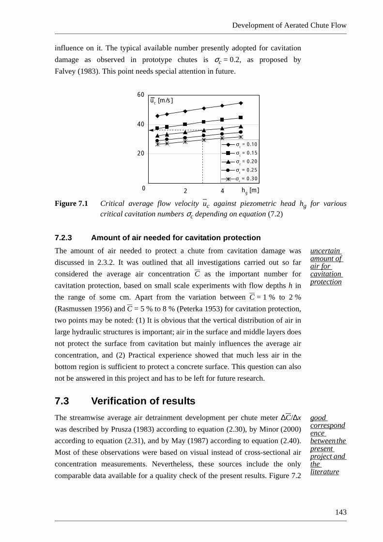
Development of Aerated Chute Flow
143
influence on it. The typical available number presently adopted for cavitation
damage as observed in prototype chutes is σc = 0.2, as proposed by
Falvey (1983). This point needs special attention in future.
Figure 7.1 Critical average flow velocity uc against piezometric head hg for variouscritical cavitation numbers σc depending on equation (7.2)
7.2.3 Amount of air needed for cavitation protection
uncertain amount of air for cavitation protection
The amount of air needed to protect a chute from cavitation damage was
discussed in 2.3.2. It was outlined that all investigations carried out so far
considered the average air concentration C as the important number for
cavitation protection, based on small scale experiments with flow depths h in
the range of some cm. Apart from the variation between C = 1 % to 2 %
(Rasmussen 1956) and C = 5 % to 8 % (Peterka1953) for cavitation protection,
two points may be noted: (1) It is obvious that the vertical distribution of air in
large hydraulic structures is important; air in the surface and middle layers does
not protect the surface from cavitation but mainly influences the average air
concentration, and (2) Practical experience showed that much less air in the
bottom region is sufficient to protect a concrete surface. This question can also
not be answered in this project and has to be left for future research.
7.3 Verification of results
good correspondence between the present project and the literature
The streamwise average air detrainment development per chute meter ∆C/∆x
was described by Prusza (1983) according to equation (2.30), by Minor (2000)
according to equation (2.31), and by May (1987) according to equation (2.40).
Most of these observations were based on visual instead of cross-sectional air
concentration measurements. Nevertheless, these sources include the only
comparable data available for a quality check of the present results. Figure 7.2
20
40
60
0 2 4
σc = 0.10
σc = 0.15
σc = 0.20
σc = 0.25
hg [m]
uc [m/s]
σc = 0.30

Chapter 7 Discussion of results
144
shows streamwise average air detrainment for a typical prototype chute for
pre-aerated flow according to equation (5.8), and aerator flow according to
equation (6.4) in comparison with the guidelines proposed by Prusza (1983),
∆C = 0.175 %/m, May (1987), ∆C(x) = Coe–0.017(xa – xi), and Minor (2000),
∆C = 0.125%/m (notation see 2.6.2). A typical straight chute was assumed with
an average inflow air concentration Co = 30 %, a specific water discharge
qw = 100 m2/s, a chute angle of α = 12.7°, and a surface roughness kst = 90 m1/
3/s. It was outlined that the aerator influences the air detrainment process by a
factor of almost three. However, the two equations for the detrainment process
from this project spans a region between aerator and pre-aeration where the
prototype observations of Prusza and May are in between and the observation of
Minor is close to it.
Figure 7.2 Average air detrainment ∆C [%] against chute distance x [m] according toequation (5.8) for pre-aerated flow () and to equation (6.4) for aerator flow(•) in comparison with literature proposals, ( ) range between aerator devicesin the present project
7.4 Summary of results
classifica-tion of the flow field
It was demonstrated in Chapter 5 and Chapter 6 that the development of air
concentration downstream of an aerator device can be classified as: (1) Inflow
with air concentrations Co and Cbo, (2) Air detrainment region C90,det and Cb,det
(3) Minimum air concentration C90,min and Cb,min, (4) Air entrainment region
C90,ent, and (5) Uniform air concentration region with C90u (Figure 5.1).
Furthermore, the air detrainment gradient det(C) describes the increase of the air
concentration contour lines C, and a bubble rise velocity ubu was derived
depending on the detrainment gradient. Table 7.1 presents the substantial results
for the mentioned quantities developed in the present project.
10
20
30
0 100 200
Prusza (1983)
May (1987)
Kramer, pre-aeration
Kramer, aerator
C [%]
x [m]
Minor (2000)

Development of Aerated Chute Flow
145
Table 7.1 Summary of the substantial results
item equation limits number
Average airdetrainment,
jetbox(5.4)
Average airdetrainment,
aerator(6.2)
Average airdetrainment per chute length ∆x,
jetbox
(5.8)
Average airdetrainment per chute length ∆x,
aerator
(6.4)
Average minimum air concentra-
tion, jetbox or aerator
Fo ≥ 6, So ≥ 10 % (5.12)
Average air entrainment, jetbox and
aerator
X90(Cmin) ≤ X90u (5.13)
Uniform air concentration
0 ≤ sinα ≤ 0.5 (5.14)
Bottom airdetrainment,
jetbox(5.19)
Bottom airdetrainment,
aerator(6.8)
C90 det, 0.0030 αsin 1–( )X90u Co+= Co C90 det, Cmin≥ ≥
C90 det, 0.0085 αsin 1–( )X90u Co+= Co C90 det, Cmin≥ ≥
∆C90 det,∆x
--------------------- 0.0030kst
qw------
35---
αsin( )310------
αsin 1–( )= Co C90 det, Cmin≥ ≥
∆C90 det,∆x
--------------------- 0.0085kst
qw------
35---
αsin( )310------
αsin 1–( )= Co C90 det, Cmin≥ ≥
Cmin 0.015Fo m– i n=
C90 ent, C90utanh d X⋅ 90u( )=
C90u13--- αsin( )0.25
=
Cb det, Cboe7.2 0.006
So 6.6+⋅( )– Fo2.50– X90u= Cbo Cb det, Cb min,≥ ≥
Cb det, Cboe30 0.006⋅
So– Fo2.50– X90u= Cbo Cb det, Cb min,≥ ≥

Chapter 7 Discussion of results
146
Table 7.2 Summary of parameters for Table 7.1
Minimum bottom air concentra-
tion, jetbox or aerator
(5.20)
Air detrain-ment gradient
(5.24)
Non-dimen-sional bubble rise velocity
(5.27)
item name meaning number
X90unon-dimensional longitudinal coordinate
X90u = x/h90u Table 4.2
h90uuniform mixture flow depth where C = 90 %
h90u = hw assumption for practical applications
Co average inflow air concentration 5.2.1
Fo-min streamwise Froude number (5.11)
F(Cmin) Froude number at inception point
Cbo inflow bottom air concentration 5.3.1
Fr(C)Froude number at the point of interception r (see Figure 5.19)
Table 5.3
detr(C)
detrainment gradient at the point of interception r (see Figure 5.19)
Table 5.3
tslope of trend line for non-dimensional bubble rise velocity
t = 0.029 Table 5.4
F0 Froude number for Ubu = 0 Table 5.4
ubu(C)
dimensional bubble rise velocity depending on the air concentra-tion
(5.26)
item equation limits number
Cb min, 3.6 107–⋅ e
0.70Fo m– i n= Fo 6 So 10%≥;≥
det C( ) 7.2 104–⋅ 2.7 αsin( )tan +( )–=
1.4 103– )⋅+ Fo Fr C( )–( ) detr C( )+⋅
Ubu o– t– Fo min– F0–( )= Fo min– 6≥
Fo min–
Fo F Cmin( )+
2--------------------------------=
ubu C( ) Ubu gho=

Development of Aerated Chute Flow
147
7.5 Discussion
amount of entrained air is not meaningful
This project investigates the behaviour of the air-water mixture flow along a
chute for several experimental set-ups. The developments of the average air
concentration C90 and the bottom air concentration Cb in streamwise direction
were shown for (1) Pre-aeration, (2) Aerator flow, and (3) Self-aeration from the
free surface. For the average air concentration and the bottom air concentration
two different effects were found. It was shown that the average air concentration
detrains quicker as the bottom air concentration and that small amounts of air
remain for a longer distance. This finding poses the question of the amount of
air actually needed to protect a chute from cavitation damage. This question
could not be answered in this project, however, it seems to be proven that the air
in the bottom region is more important than the average air concentration. Most
projects conducted up till now concentrated on the development of the average
air concentration and on the design of the aeration device and thus on the
amount of entrained air Co. The results for the average air concentration
developed in the present project were comparable to that found on prototypes. It
was furthermore shown that the amount of air is not meaningful for the total
chute reach to be protected. The aerator geometry seems to influence the air
detrainment behaviour strongly by a factor of almost three. This can be
explained by a non-hydrostatic pressure gradient in the impact zone, which
presses the air out of the flow and leads to a larger air detrainment. However,
only one aerator geometry was examined in addition to jetbox flow. Therefore,
more research is needed in this near aerator field.
equilib-rium flow conditions
The knowledge of the uniform flow characteristics of air-water flows may
seem to be of academic character, given that usual chutes have a length of some
hundreds of meters (e.g. x = 300 m). With a assumed uniform flow depth of 1 m
to 5 m, the relative length thus amounts between Xu = 300/5 = 60 to Xu = x/
hu = 300/1 = 300. Considering Figure 5.1 for instance, such relative lengths
were observed also during the present project. In practice, one would
furthermore argue that chutes have hardly a constant bottom slope, given the
topographical site conditions. The concept of uniform flow in hydraulics is of
limited immediate interest. However, it corresponds to the flow situation by
which most flow conditions are scaled because it can be calculated exactly
(Kramer et al. 2003).
expansion of the present knowledge
Today, the knowledge on the equilibrium flow conditions for chutes is
limited. The basic data sets available include those of Straub and
Anderson (1960) for a non-specified roughness, the data of Anderson (1965) for

Chapter 7 Discussion of results
148
a practically smooth chute boundary which was also not specified, and some
additional data of the Indian research program basically carried out by
Gangadharaiah et al. (1970). Wood (1991), for instance, was unable to specify
these conditions, although he had directed a considerable number of research
projects in that domain. It must therefore be stated that we do actually not know
the effects of boundary roughness on the uniform two-phase flow conditions on
chutes. The air entrainment observed for the present boundary conditions
particularly for the chute roughness of ks = 0.00023 mm was hardly sufficient to
protect a chute surface from cavitation damage. Although a large quantity of air
was entrained from the free surface and influenced the average air concentration
substantially, the bottom air concentration was almost not effected.
Accordingly, research programs have to be directed to that delicate hydraulic
problem.
a first step in the right direction
Nevertheless open questions relating to the critical cavitation number σc for
initial cavitation damage, and the critical amount of air needed to protect a chute
from cavitation damage Ccrit must be answered. The present research may be
considered a first step in that direction.
7.6 Design example
7.6.1 General comment
hydraulic on a prototype chute
This section aims to demonstrate a design procedure for a chute in order to
explain the application of the developed equations for practice. This project
concentrated on the air detrainment part downstream of an aerator, therefore,
the procedure is linked to a project regarding the air entrainment of an aerator.
Due to limited space the hydraulic part of the chute system is kept short and
only one discharge is considered here. It was already outlined that the design
engineer must find the critical flow conditions and thus has to consider a
number of typical discharge cases.
The first steps follow the well known design procedure for aerator design on
a chute as mentioned, e.g. by Rutschmann (1988) or Falvey (1990).
design the chute
1. Consider the topography, the dam structure and the maximum
discharge Qmax to design the auxiliary structures such as the chute, the
bottom outlet, the energy dissipator, etc.
critical points
2. Find the critical points in the chute system such as negative curvature,
surface irregularities, concrete joints, etc.

Development of Aerated Chute Flow
149
cavitation number
3. Study the cavitation characteristics of the structure to find the critical
conditions by means of the cavitation number σ (2.1). In lack of better
information follow the guidelines proposed by Falvey (1990) for
surface offset tolerances as a function of the minimum cavitation
number σ.
critical cavitation number
4. For critical cavitation numbers σc ≤ 0.2 investigate the effect of
changes to the chute geometry on the cavitation number. If low values
of the cavitation number cannot be modified, an aerator devices must
be located at the point where the cavitation number falls below the
critical value σ ≤ σc = 0.2.
point of inception
5. Calculate the location of the inception point xi using one of the
equations (2.5), (2.6), or (2.7), respectively. Determine the average air
entrainment C90,ent downstream of xi according to (5.15); downstream
of the point C90,ent = Ccrit ≈ 25 % it is supposed that the bottom air
concentration exceeds its minimum number Cb,min ≥ Cb,crit ≈ 1.0 %
and thus no aerator is needed. Note that for far smaller average air
concentrations the chute might also be protected. This, however, is an
assumption which has to be clarified (see also 2.4.2).
design of an aerator device
6. Follow one of the proposed design procedures for aerator devices, e.g.
Koschitzky (1987), Chanson (1988), Rutschmann (1988),
Falvey (1990), Balaguer (1992), or Skripalle (1994). Note that the
optimum aerator design for the chute to be protected must not
necessarily be the aerator associated with the highest amount of inflow
air Co but the aerator with the minimum shock waves and pressure
peaks in the impact zone.
minimum air concentra-tion
7. Find the Froude number Fo at the aerator device and the Froude
number F(Cmin) at the point of inception xi. Determine the streamwise
Froude number Fo-min according to equation (5.11). Use equation
(5.12) for the average minimum air concentration Cmin and equation
(5.20) for the minimum bottom air concentration Cb,min. For
Cmin ≥ Ccrit ≈ 5 % and Cb,min ≥ Cb,crit ≈ 1.0 %, respectively, no
additional aerator is needed provided the chute slope So is constant.
air detrain-ment downstr. of the aerator device
8. The streamwise average air detrainment C90,det can be calculated
according to equation (5.4) for conditions similar to jetbox flow
indicating an optimum air concentration distribution over the flow
depth. Because the aeration device was not subject of this project, the

Chapter 7 Discussion of results
150
air detrainment downstream of an aerator similar to that used in the
present project can be determined according to equation (6.2).
However, since no general design guideline was proposed for various
aerator devices, this question is left to future reserach. The air
detrainment downstream of an aerator will behave in fact somewhat
between jetbox and aerator flow. If the average air concentration falls
below Cmin = Ccrit ≈ 5 % a second aerator is required if the bottom air
concentration falls below the critical value (see below).
bottom air concentra-tion
9. Compute the bottom air detrainment Cb,det according to equation (5.4).
For a bottom air concentration Cb,min ≤ Cb,crit ≈ 1.0 % a second aerator
must be added.
loop 10. Repeat steps 5 through 9 until all aerators are located and designed.
7.6.2 Design procedure – an example
Details
chute hydraulics and flow details
The design procedure is performed for an example proposed by
Koschitzky (1987) who concentrated on the aeration and aerator device. Figure
7.3 shows details of the chute with a maximum discharge capacity
Qmax = 3300 m3/s. The bottom slope is So = 30 % with a concrete made chute
surface of surface roughness kst = 80 m1/3/s. Hydraulic calculations of the most
important parameters, flow depth h(x), flow velocity uw(x), Froude number
F(x), and cavitation number σ(x) are shown in Figure 7.3. Koschitzky suggested
to locate two aerators at x = 125 m where the critical cavitation number is
σc = 0.25, and at x = 175 m with the spacing calculated according to equation
(2.30) with the average air detrainment ∆C = 0.2 % per meter (Prusza1983).
Note that a critical cavitation number of σc = 0.20 should be safe enough. For
better comparison between Koschitzky’s and this example, the first aerator is
also placed at x = 125 m.
Problem
determine the aerator spacing!
Calculate the behaviour of the air-water flow downstream of the first aerator,
based on the hydraulic calculations of Koschitzky (1987). Determine whether a
second aerator is needed and the aerator spacing of a second aerator at the point.
Consider a critical average air concentration below Ccrit = 5 % and a critical
bottom air concentration below Cb,crit = 1.0 %. Both demands must be meet.

Development of Aerated Chute Flow
151
a)
b)
Figure 7.3 Computational example a) Sketch of chute including main dimensions, andb) streamwise black water profile h(x), average flow velocity u(x), Froudenumber F(x), and cavitation number σ(x) (Koschitzky 1987)

Chapter 7 Discussion of results
152
Solution
general design
• Points 1. to 4. from the general design procedure are shown in Figure
7.3.
point of inception
• The point of air inception is at xi = 143.2 m where the thickness of the
turbulent boundary layer is equal to the flow depth with δ = hi = 2.4 m,
according to the iterative equation (2.6) δ/xi = 0.0212•0.290.11(80/
xi)0.10 (Wood et al. 1983). Note that other equations for the point of
inception may yield other results.
air entrain-ment
• The air entrainment downstream of the point of inception can be
described according to equation (5.15) with
C90,ent = 0.33•0.290.25tanh(0.004•107/2.2) = 4.6 % at x = 250 m with
hu = 2.2 m and d = 0.004 for pre-aerated flow conditions. This result
indicates that the air concentration downstream of the inception point
will not be sufficient for the minimum required number
C90u = 4.6 % ≤ Ccrit ≈ 5 %.
minimum air concentra-tion
• The streamwise Froude number is Fo-min = (6.1 + 6.5)/2 = 6.3
according to equation (5.11). With equation (5.12) the average
minimum air concentration yields Cmin = 0.015•6.3 = 0.11 = 11 %
which is above the critical value Cmin = 11.5 % ≥ Ccrit ≈ 5 %. The
minimum bottom air concentration Cb,min = 3.6•10–7e0.70•6.3 =
4.9•10–5 according to equation (5.20) is much smaller than
Cb,min = 4.9•10–5 ≤ Cb,crit ≈ 1.0 %, therefore a second aerator is
required.
average air detrain-ment
• The streamwise average air detrainment is C90,det = 0.0085(0.29 –
1)(x – 125)/2.2 + 0.09 = –0.0027(x – 125) + 0.09 according equation
(6.2). With C90,det = Ccrit = 5 % at the distance x = (0.05 – 0.09)/(–
0.0027) + 125 = 139 m a second aerator is needed, if the bottom air
concentration reduces also below its critical value.
bottom air detrain-ment
• The bottom air concentration can be calculated according to equation
(6.8) to Cb,det = 0.05e–(30•0.006^0.3)•6.1^–2.50•(x – 21.0 – 125)/2.2 = 0.05e–
0.032(x – 21.0 – 125). In this equation the two assumptions are added, a
trajectory length of lt = 21.0 m as proposed by Koschitzky and a
characteristic bottom air concentration of Cbo = 0.05 at the point of jet
impact. The equation can be solved to obtain the distance to the second

Development of Aerated Chute Flow
153
aerator at x = –ln(0.01/0.05)/0.032 + 125 + 21.0 = 196.0 m where the
bottom air concentration falls below Cb,crit = 1.0 %. This is the
distance downsteam of the inflow at x = 0, the distance downstream of
the aerator protected by air is x = 196 - 125 = 71 m.
• The behaviour of the air concentration downstream of the second
aerator can be calculated as above. However, no third aerator is needed
over the remaining chute reach of ∆x = 250 – 196 = 54 m.
• Note that the above example involves calculations with respect to
aerator measurements, deviations may occur for pre-aerated flow
calculations, as outlined. Since only one aerator geometry was
investigated, it is supposed that a better geometry can extend the
protected chute distance. The truth for an optimum aerator will be
somewhere between pre-aeration and aerator measurements.
extended aerator spacing
This general example shows that the aerator spacing can be extended from
∆x = 42 m (Koschitzky 1987) to ∆x = 71 m for the flow conditions adopted.
Note that the average air concentration falls below the critical value Ccrit ≈ 5 %
after only 35 m downstream of the aerator because of the small air entrainment
from the aerator of only Co = 9 %, as determined by Koschitzky. Furthermore,
the average air entrainment from the free surface C90,ent = 4.7 % is insignificant
for cavitation protection at the end of the chute of (250 – xi) = 107 m
downstream of the point of inception xi. This is an interesting point, because the
self entrainment seems not to protect a chute within a common chute length for
the considered chute slope of So = 30 %. Figure 7.4 shows the streamwise
development of the average air detrainment C90, the surface air entrainment
C90,ent, and the bottom air concentration Cb. The average air concentration is
shown linearly up C90 = 15 % in Figure 7.4a and the bottom air concentration
semi-logarithmically between 0.01 % ≤ Cb ≤ 1.0 in Figure 7.4b. The average
and the bottom air concentrations rise at x = 125 m within a trajectory length of
lt = 21.0 m to C90 = 9.0 % and to Cb = 100 %, respectively. Downstream from
this location the air detrains as calculated above, before air is entrained again
from the second aerator at x = 196 m. The average air concentration reduces to
C90 = 0 at x = 180 m disregarding the minimum value for such flows.
Furthermore, free surface entrainment can be observed starting from xi = 143 m
Figure 7.4c. The free surface entrainment follows a tangent hyperbolic function
although it appears to be linear. The sum of the air entrained from the aerator

Chapter 7 Discussion of results
154
and the free surface provides the absolute amount of average air concentration.
The bottom concentration falls from Cb = 100 % in the cavity to Cb = 5 %
immediately downstream of it, due to pressure peaks in this region. The
remaining bottom air concentration reduces to Cb = 1 % at x = 196 m where the
second aerator was located. The same process repeats again.
a)
b)
0.05
0.10
0.15
0100 200
trajectorytrajectory
aerator 1x = 125.0 m
aerator 2x = 196.0 m
aver
age
air
conc
entr
atio
n
C90
x [m]
C90,det
C90,det
Ccrit
100 200
10-4
10-3
10-2
10-1
1
Cb,min = 1 %
trajectoryCb
botto
m a
ir co
ncen
trat
ion
aerator 1x = 125.0 m aerator 2
x = 196.0 m
x [m]
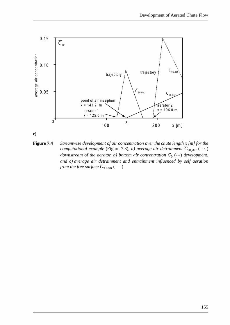
Development of Aerated Chute Flow
155
c)
Figure 7.4 Streamwise development of air concentration over the chute length x [m] for thecomputational example (Figure 7.3), a) average air detrainment C90,det (-·-·-)downstream of the aerator, b) bottom air concentration Cb (---) development,and c) average air detrainment and entrainment influenced by self aerationfrom the free surface C90,ent (–––)
0.05
0.10
0.15
0100 200
trajectory trajectory
aerator 1x = 125.0 m
aerator 2x = 196.0 m
xi
point of air inceptionx = 143.2 m
aver
age
air
conc
entr
atio
n
C90
x [m]
C90,det
C90,det
C90,ent

Chapter 7 Discussion of results
156

Development of Aerated Chute Flow
157
CHAPTER 8 CONCLUSIONS
8.1 Limitations and results
The behaviour of air-water flow was investigated on a chute model with two
distinctly different air supply devices for air-water flow generation. The
limitations and results of the experimental investigations and the theoretical
developments can be summarised as:
Limitations
altered parameters
• The inflow Froude number was varied between 3 ≤ Fo ≤ 14, the inflow
depth between 0.05 m ≤ ho ≤ 0.12 m, the chute slope between
0 % ≤ So ≤ 50 %, and the inflow air concentration between
0 ≤ Co ≤ 30 %. All quantities were varied for two distinctly different
air supply devices: (1) Aerator flow, similar to a prototype, and (2)
Pre-aeration by adding air to the supply pipe.
physical model and data accuracy
• A remote controlled positioning system was successfully applied
carrying the automated fiber-optical instrumentation. A large number
of measurements was conducted to cover a wide range of streamwise
two-phase chute flow conditions along the 14 m chute model of
variable bottom slope, variable inflow depth, and variable discharge.
The data collection grid for one run was based on 665 local points with
an increasing spacing in the streamwise direction. The accuracy of the
air concentration measurements was found to be in a tolerance of
± 5 %.
non-dimensional parameter
• The following non-dimensional quantities for a 2D-model were
considered relevant: The Froude number F = Qw/(gb2h3)1/2 for mixture
(subscript m) and pure water (subscript w) flow depth, the streamwise
averaged Froude number Fo-min = (Fo + F(Cmin))/2, the non-
dimensional streamwise coordinate X90u = x/h90u, the non-dimensional
transverse coordinate Z90u = z/h90u, the air detrainment gradient
det(C) = dX90u/dZ90u, and the non-dimensional bubble rise velocity
Ubu = ubu/(gh)1/2.

Chapter 8 Conclusions
158
Results
gap in the present knowledge
• Three problems were outlined in the literature review for cavitation
protection on chutes: (1) Unspecified quantities of air and its vertical
distribution needed for cavitation protection on a chute, (2) The critical
cavitation number for cavitation inception, and (3) The behaviour of
the air downstream of an air supply device which is not yet understood.
Point three was investigated in this project.
qualitative description of the flow field
• This project presents the first systematical measurements of air
concentration in high-speed chute flows. Five typical regions describe
the air-water flow qualitatively: (1) Inflow region, (2) Air detrainment
region, (3) Minimum air concentration region, (4) Air entrainment
region, and (5) Uniform mixture flow region. These findings disagree
with earlier statements where the inflow air concentration was assumed
to pass directly in the uniform region.
average air detrain-ment
• Average air detrainment in the region between a given inflow and the
minimum air concentration can be calculated for pre-aerated flow
according to equation (5.4) and for aerator flow according to equation
(6.2). The air detrains linearly depending on the chute angle and the
inflow air concentration. A three times larger detrainment gradient was
found for aerator flow compared to pre-aeration, wich was explained
by the highly non-hydrostatic pressure gradient in the point of impact.
Based on this finding two equation were derived to describe the air
reduction per distance ∆x. Here the specific discharge and the
roughness coefficient kst was found to be the important quantities. It
was demonstrated that the average air detrainment per chute meter
follows also a linear function including the chute slope and have the
same range of air detrainment as observations made on prototypes.
aerator design must reduce pressure peaks
• The quantity of air supplied by air ducts is not always an important
design parameter in terms of aerator efficiency. The aerator geometry
has to be optimised to reduce high pressure gradients in the impact
zone, rather than focusing on the quantity of air supplied into the flow.
average minimum air concentra-tion
• The average minimum air concentration for both pre-aerated and
aerator flow was found to be a function of the streamwise development
of the Froude number. It was shown that for certain flow conditions the
average minimum air concentration never falls below a critical value,
thus one aerator is sufficient to protect a chute from cavitation damage.

Development of Aerated Chute Flow
159
air entrain-ment
• Downstream of the point of inception the average air concentration
develops following a tangent hyperbolic function. A typical fan-shaped
behaviour of the air concentration contour lines downstream of the
inception point was shown. It was thus proven that a full cavitation
protection by air from the free surface begins far downstream of the air
inception point.
uniform air concentra-tion
• The uniform air concentration in the present project was described by a
power function depending on the chute angle only. This finding was
similar to that in the literature, based on Straub and Anderson’s (1958)
classical data set.
bottom air detrain-ment
• The bottom air concentration was found to be the most meaningful
quantity for cavitation protection on chutes. The air detrainment
process follows for both air supply methods an exponential trend
depending on the inflow Froude number, the chute slope, and the
inflow bottom air concentration. The bottom air concentration for
pre-aerated flow reduces exponentially between the inflow and the
minimum locations, whereas the air detrainment for aerator flow must
be separated in the near and the far flow field in which the first is
affected from the aerator.
minimum bottom air concentra-tion
• It was mentioned that the bottom air concentration does not fall below
a minimum value for certain flow conditions. The exponential function
of the minimum air concentration is mainly influenced by the
streamwise averaged Froude number.
air detrain-ment gradient
• A new method was developed to describe the air detrainment with
respect to the increasing air concentration contour lines C = 1.0 % and
C = 0.1 %. The air detrainment gradient is a function of various
parameters primarily depending the chute angle.
bubble rise velocity
• The bubble rise velocity was derived from the air detrainment
gradients. This indirect method gives an order of magnitude of air
bubble rise in high-turbulent flow conditions.
influence of the air supply system
• The air detrainment for the two air supply systems, namely: (1) Aerator
flow, and (2) Pre-aeration, varied by a factor of almost three. This is
due to the difference in the pressure gradient at the point of jet impact
in aerator flow. Further research was proposed in this field.
practical calcula-tions
• Practical examples demonstrated that the present results can be used to
calculate the streamwise behaviour of the average and the bottom air
concentrations, provided the inflow conditions are specified and the
limitations mentioned in the equations are respected.

Chapter 8 Conclusions
160
8.2 Outlook
two open questions
This project analysed the streamwise air concentration development on a chute
model. There are still two open questions: (1) The minimum amount of air
needed for cavitation protection, and (2) The critical cavitation number σc.
Furthermore, more research is needed to find an optimum aerator design. Here,
attention should be paid to minimise the pressure in the impact zone rather than
concentrate on the absolute amount of entrained air.
extend the chute slope, discharge, and channel roughness
Data for steeper slopes may be desirable especially to investigate the free
surface entrainment and the uniform mixture flow region. A higher discharge or
prototype investigations are always preferable to reduce scale effects. This may
be achieved by halving the chute width, yet, air entrainment from the boundary
wall and shock waves then may influence the measurements. The effect of chute
roughness was not included in this study. A higher air concentration is expected
for a rougher channel surface, similarly to the results provided by Straub and
Anderson (1958).

Development of Aerated Chute Flow
161
NOTATION
A m2 cross-sectional area of the flow
b m chute width
B – Boussinesq number B = u/(gRh)1/2
= f(F, geometry)
c m/s sonic velocity
C – local air concentration by volume
Cb – bottom air concentration
Cbo – upstream bottom air concentration
Cmin – average minimum air concentration at
the point of inception
Co – average inflow air concentration
C90 – average air concentration
C90u – average uniform air concentration
dbu mm bubble diameter
det(C) – air detrainment gradient det(C) = dZ90u/dX90u
F – Froude number F = Qw/(gb2hw3)1/2
Fc – critical Froude number for beginning
air entrainment
Fo – inflow Froude number Fo = Qw/(gb2ho3)1/2
Fo-min – streamwise Froude number Fo-min = (Fo + F(Cmin))/2
g m/s2 Gravity acceleration g = 9.81 m/s2
h m flow depth
hc m critical flow depth
hg m piezometrical pressure height
ho m inflow depth at the jetbox
hi m flow depth at the point of inception
hu m uniform flow depth
C901
h90------- C z( ) zd
0
h90
=

Chapter 8 Conclusions
162
hw m water depth
h90 m mixture flow depth where C = 90 %
h95 m mixture flow depth where C = 95 %
h99 m upper flow depth reached by water
droplets
h90u m uniform mixture flow depth, if no
better information are available
h90u = hwu
Hs m difference of water surface elevations
between inception point and reservoir
level
ks mm equivalent sand roughness height
according to Nikuradse
kst m1/3/s roughness coefficient
L m length of the trajectory of the
impigning jet
l m chute length b = 14 m
lr m aerator length lr = 150 m
lu m wetted perimeter
m – bottom air detrainment gradient
P – Prandtl number R = τw/(u2•ρw)
pa N/mm2 local air pressure
po N/mm2 local pressure po = pA + pg
pA N/mm2 Atmospheric pressure po ≈ 1014 hPa
= 0.1014 N/mm2
pg N/mm2 gauge pressure 1N/mm2
102 m water column
pv N/mm2 vapour pressure of liquid pv = 16.0 hPA
= 0.0016 N/mm2 (14°C)
qw m3/s specific water discharge
Qa m3/s air discharge
Qw m3/s water discharge
R – Reynolds number R = uhw/νw
hw 1 C z( )–( ) zd
0
h90
=
=

Development of Aerated Chute Flow
163
R2 – statistic correlation
parameter
R-square
Rh m hydraulic radius Rh = A/lu
So – chute slope (tanα) 0 % ≤ So ≤ 50 %
SE – slope of energy
ta – acquisition time
tr mm aerator height tr = 15 mm
Tu – turbulence intensity
u m/s local flow velocity
u m/s average flow velocity u = Q/(bh)
ua m/s air velocity
ubu m/s bubble rise velocity
Ubu – non-dimensional bubble rise velocity Ubu =ubu/(gho)0.5
Ulow V lower treshold
Uup V upper treshold
u90 m/s flow velocity where C = 90 %
U90 – non-dimensional flow velocity U90 = u/u90
v’ m/s turbulent velocity fluctuations
W – Weber number W = uw/(σt/(ρdbu))1/2
x m coordinate originate at the jetbox
xi m distance from the spillway crest to the
point of inception
xs m distance from the spillway crest
Xo – non-dimensional inflow distance Xo = x/ho
Xshift – the parameter shifts the curve on the
inflow air concentration
Xshift = (Co – 0.40)/a
X90u – non-dimensional flow distance X90u = x/h90u
y m coordinate originate at the left side
wall
z m vertical coordinate perpendicular to
the chute bottom
Zo – non-dimensional inflow depth Zo = z/ho
Tu
1n--- ui
2
i 1=
n
u
-----------------------------v'
u---= =

Chapter 8 Conclusions
164
Z90u – non-dimensional uniform flow depth Z90u = z/h90u
Greek symbols
α ° spillway slope (arctanSo)
β – ratio of volumetric aerator inflow rate β = Qa/Qw
δ m turbulent boundary layer thickness
λ – scaling length
ρ kg/m3 density of water ρ = 1000 kg/m3 (4°C)
ν m2/s kinematic viscosity
σ – cavitation number σ = (po – pv)/(ρu2/2)
σc – critical cavitation number
σd – standard deviation
σt N/m interfacial surface tension between air
and water
τo kg/(ms2) wall shear stress
µ kg/(ms) dynamic viscosity
Subscr ipt
a air
b bottom
bu bubble
c critical
det detrainment
dr computed value for equilibrium flow,
using Manning’s equation for pure
water
ent entrainment
g gauge pressure
i at point of inception
m mixture
min,
max
minimum and maximum
o inflow conditions

Development of Aerated Chute Flow
165
u uniform flow conditions equivalent to
the measured flow parameter at the
downstream end of the chute
w water
90 C = 90 %
95 C = 95 %
99 C = 99 %

Chapter 8 Conclusions
166

Development of Aerated Chute Flow
167
REFERENCES
Anderson, A.G. (1965). Influences of channel roughness on the aeration of high-velocity, open-
channel flow. 11. IAHR Congress, Leningrad 1.37: 1-13.
André, S., Boillat, J.-L. and Schleiss, A. (2001). High velocity two-phase turbulent flow over
macro-roughness stepped chutes: Focus on dynamic pressures. 3 International Symposium
on Environmental Hydraulics, Tempe, Arizona, CD-Rom.
Arndt, R.E.A. (1977). Cavitation from surface irregularities in high velocity flow. Journal of
the Hydraulics Division, ASCE, 103(HY4): 469-472.
ASCE/USCOLD. (1975). Lessons from dam incidents, USA. The Committee on Failures and
Accidents to Large Dams. ASCE, New York.
Azzopardi, B.J. (1999). Turbulence modification in annular gas/liquid flow. International
Journal of Multiphase Flow 25: 945 - 955.
Bachmeier, G. (1988). Aufbau, Eichung und Einsatz einer Messsonde zur Bestimmung der
Luftblasenkonzentration in einer Schussrinne. Diploma Thesis, Institut für
Hydromechanik, Technische Universität, Karlsruhe (in German, unpublished).
Ball, J.W. (1977). Cavitation from surface irregularities in high velocity. Journal of the
Hydraulics Division, ASCE, 102(HY9): 1283-1297.
Balaguer, G. (1993). Sohlenbelüfter in Schussrinnen ergänzende Untersuchungen zur
Bemessung. Institut für Wasserbau und Kulturtechnik, Universität Fridericiana, Karlsruhe
(in German).
Bauer, W.J. (1954).Turbulent boundary layer on steep slopes. Trans. ASCE 119: 1212-1242.
Boes, R. (2000a). Zweiphasenströmung und Energieumsetzung an Grosskaskaden. VAW
Mitteilung 166. Versuchsanstalt für Wasserbau, Hydrologie und Glaziologie. ETH, Zürich
(in German).
Boes, R. (2000b). Scale effects in modelling two-phase stepped spillway flow. Hydraulics of
stepped spillways 53-67, H.-E.Minor and W.H. Hager, eds. Balkema, Rotterdam.

Chapter 8 Conclusions
168
Boes, R. and Hager, W.H. (1998). Fiber-optical experimentation in two-phase cascade flow.
Intl. RCC Dams Seminar, Denver, CD-Rom.
Boes, R. and Hager, W.H. (2003). Two-phase flow characteristics of stepped spillways.
Journal of Hydraulic Engineering 129(9): 661-670.
Bormann, K. (1968). Der Abfluss in Schussrinnen unter Berücksichtigung der Luftaufnahme.
Bericht 13. Versuchsanstalt für Wasserbau. Technische Universität, München (in German).
Bradley, J.N. (1945). Study of air injection into the flow in the Boulder dam spillway tunnels -
Boulder Canyon Project. Report HYD-186, Bureau of Reclamation, Denver.
Braeske, H., Domnick, J. and Brenn, G. (1997). Experimentelle Grundlagenuntersuchungen
zur Strömungsmechanik in Blasensäulen. Report LSTM 552/E97. Lehrstuhl für
Strömungsmechanik, Technische Fakultät der Friedrich-Alexander-Universität, Erlangen-
Nürnberg (in German).
Bretschneider, H. (1989). Der Beginn des Lufteintrages bei Sohlennischen mit Rampe.
Wasserwirtschaft 79(4): 180-185 (in German).
Bruschin, J. (1987). Forced aeration of high velocity flows. Journal of Hydraulic Research
25(1): 5-14.
Cain, P. (1978). Measurements within self-aerated flow on a large spillway. Report 78-18.
University of Canterbury, Christchurch.
Cartellier, A. and Achard, J.L. (1991). Local phase detection probes in fluid/fluid two-phase
flows. Rev. Sci. Instrum. 62(2): 279-303.
Chanson, H. (1988). Study of air entrainment and aeration devices on spillway model. Report
88-8. University of Canterbury, Christchurch.
Chanson, H. (1989). Flow downstream of an aerator - aerator spacing. Journal of Hydraulic
Research 27(4): 519-536.
Chanson, H. (1994). Drag reduction in open channel flow by aeration and suspended load.
Journal of Hydraulic Research 32(1): 87-101.
Chanson, H. (1997). Air bubble entrainment in free-surface turbulent shear flows. Academic
Press, Brisbane.
Chanson, H. and Toombes, L. (2002). Air-water flows down stepped chutes: Turbulence and
flow structure observations. International Journal of Multiphase Flow 28: 1737-1761.

Development of Aerated Chute Flow
169
Colgate, D. (1976). Hydraulic model studies of Amaluza dam spillway. Report GR-25-76 65.
Bureau of Reclamation, Denver.
Comolet, R. (1979). Sur le mouvement d'une bulle de gaz dans un liquide. La Houille Blanche
35(1): 31-42.
Drewes, U. and Aksoy, S. (1992). Prototype measurements at an aerator of the Randenigala
spillway chute, Sri Lanka. International Symposium on Cavitation and Erosion in
Hydraulic Structures and Machinery, Nanjing, 126-136.
Ehrenberger, R. (1926). Wasserbewegung in steilen Rinnen (Schusstennen) mit besonderer
Berücksichtigung der Selbstbelüftung. Zeitschrift des Österreichischen Ingenieur- und
Architekten-Vereins 78(15/16): 155-160; 78(17/18): 175-179 (in German).
Eigenberger, G. (1997). Experimentelle Untersuchung von Gas-Flüssigkeits-Reaktoren mit
Blasenauftriebsströmung. Report EI 131/9-3. Institut für Chemische Verfahrenstechnik,
Technische Universität, Stuttgart (in German).
Eisenhauer, N. (1993). Der Einfluss der Belüftung auf die Kavitationserosion. Mitteilung 183.
Institut für Wasserbau und Kulturtechnik, Universität Fridericiana, Karlsruhe (in German).
Eisenhauer, N. (1995). Die Reduzierung der Kavitationserosion durch Belüfter.
Wasserwirtschaft 85: 80-84 (in German).
Elder, R.A. (1986). Advances in hydraulic engineering practice: The last four decades and
beyond. Journal of Hydraulic Engineering 112(2): 74-89.
Ervine, D.A. and Falvey, H.T. (1987). Behaviour of turbulent water jets in the atmosphere and
in plunge pools. Proc. Instn. Civ. Engineers 33(2): 295 - 314.
Ervine, D.A., Falvey, H.T. and Kahn, A.R. (1995). Turbulent flow structure and air uptake at
aerators. Hydropower & Dams 2(4), 89-96.
Falvey, H.T. (1980). Air-water flow in hydraulic structures. Engineering Monograph 41,
Bureau of Reclamation, Denver.
Falvey, H.T. (1983). Prevention of cavitation on chutes and spillways. Frontiers in hydraulic
engineering 432-437, H.T. Shen, ed. Massachusetts Institute of Technology, Cambridge.
Falvey, H.T. (1990). Cavitation in chutes and spillways. Engineering Monograph 42, Bureau
of Reclamation, Denver.
Falvey, H.T. and Ervine, D.A. (1988). Aeration in jets and high velocity flows. Model-
Prototype Correlation of Hydraulic Structures, Colorado Springs, Colorado, 25-55.

Chapter 8 Conclusions
170
Frizell, K.W. (1988). Chute spillway aerators - McPhee dam model/prototype comparison.
Model-Prototype Correlation of Hydraulic Structures, Colorado Springs, Colorado, 129-
137.
Gal'perin, R.S., Oskolov, A.G., Semenkov, V.M. and Tsedrov, G.N. (1979). Cavitation in
hydraulic structures. Report UDC 627.8: 532.528. Energiya, Moscow.
Gangadharaiah, T., Lakshmana Rao, N.S. and Seetharamiah, K. (1970). Inception and
entrainment in self-aerated flows. Journal of the Hydraulics Division, ASCE 96(HY7):
1549-1565.
Gaskin, S., Aubel, T. and Holder, G. (2003). Air demand for a ramp-offset aerator as a function
of spillway slope, ramp angle and Froude number. 30 IAHR Congress, Thessaloniki,
Theme D: 719-724.
Grein, H. (1974). Cavitation - An overview. Technische Rundschau SULZER, Escher Wyss,
Zürich
Grein, H. and Minor, H.-E. (2002). Reduktion von Kavitation durch Luft. – Personal
communication.
Haberman, W.L. and Morton, R.K. (1956). An experimental study of bubbles moving in
liquids. Trans. ASCE 121: 227-252.
Haerter, A. (1961). Theoretische und experimentelle Untersuchungen über die
Lüftungsanlagen von Strassentunneln. PhD Thesis 3024, Institut für Aerodynamik. ETH,
Zürich (in German).
Hager, W.H. (1988). Abflussformeln für turbulente Strömungen. Wasserwirtschaft 78(2): 79-
84 (in German).
Hager, W.H. (1991). Uniform aerated chute flow. Journal of Hydraulic Engineering 117(4):
528-533.
Hager, W.H. (1992). Spillways shock waves and air entrainment. ICOLD Bulletin 81,
Committee on Hydraulics for Dams, ICOLD, Paris.
Hager, W.H. and Blaser, F. (1997). Drawdown curve and incipient aeration for chute flow.
Canadian Journal of Civil Engineering 25: 467-473.
Hager, W.H. and Kramer, K. (2003). Historical development of free surface chute aeration. 30
IAHR Congress, Thessaloniki, Theme E: 389-396.

Development of Aerated Chute Flow
171
Halbronn, G., Durand, R. and Cohen De Lara, G. (1953). Air entrainment in steeply sloping
flumes. 5th IAHR Congress, Minnesota, Minneapolis, 455-466.
Hall, L.S. (1943). Open channel flow at high velocities. Trans. ASCE 108: 1393-1434; 108:
1494-1516.
Hamilton, W.S. (1983). Preventing cavitation damage to hydraulic structures. Water Power &
Dam Construction 35(11): 40-43; 35(12): 48-53.
Hamilton, W.S. (1984). Preventing cavitation damage to hydraulic structures. Water Power &
Dam Construction 36(1): 42-45.
Hammitt, F.G. (1972). Effects of gas content upon cavitation inception, performance, and
damage. Journal of Hydraulic Research 10(3): 259-290.
Hammitt, F.G. (1980). Cavitation and multiphase flow phenomena. McGraw-Hill, New York.
Hinze, J.O. (1975). Turbulence. McGraw-Hill, New York.
Ivicsics, L. (1975). Hydraulics models. Dr. Stelczer Károly, Budapest.
Jahnke, H. (1982). Die Kavitationserosion des Betons. Wasserwirtschaft-Wassertechnik, 32(7):
242-245.
Jin, T., Liu, C. and Liu, X. (1980). Cavitation inception of gate slots. Scientific Report.
Department of Hydraulics, Water Conservancy and Hydro-Electric Power, Beijing.
Keller, R.J. (1972). Field measurements of self-aerated high speed open channel flow. PhD
Thesis. University of Canterbury, Christchurch.
Kells, J.A. and Smith, C.D. (1991). Reduction of cavitation on spillways by induced air
entrainment. Canadian Journal of Civil Engineering 18: 358-377.
Kobus, H. (1974). Anwendung der Dimensionsanalyse in der experimentellen Forschung des
Bauingenieurwesens. Die Bautechnik 51(3): 88-94 (in German).
Kobus, H. (1984). Local air entrainment and detrainment. Symposium on Scale Effects in
Modelling Hydraulic Structures 4.10: 1-10, H. Kobus, ed. Esslingen am Neckar.
Kobus, H. (1985). An introduction to air-water flows in hydraulics. Mitteilung 61. Institut für
Wasserbau, Technische Universität, Stuttgart.
Kobus, H. (1991). Introduction to air-water flows. IAHR Hydraulic Structures Design Manual
4, Air entrainment in free-surface flows 1-28, I.R.Wood, ed. Balkema, Rotterdam.

Chapter 8 Conclusions
172
Kobus, H. and Koschitzky, H.-P. (1991). Local surface aeration at hydraulic structures. IAHR
Hydraulic Structures Design Manual 4, Air entrainment in free-surface flows 29-54, I.R.
Wood, ed. Balkema, Rotterdam.
Kökpinar, M.A. (1996). Air-entrainment in high speed free surface flows. PhD Thesis.
Department of Civil Engineering, Middle East Technical University, Ankara.
Koschitzky, H.-P. (1987). Dimensionierungskonzept für Sohlenbelüfter in Schussrinnen zur
Vermeidung von Kavitationsschäden. Mitteilung 65. Institut für Wasserbau, Technische
Universität, Stuttgart (in German).
Koschitzky, H.-P. (1988). Dimensionierung von Schussrinnenbelüftern. Wasserwirtschaft
78(5): 220-228 (in German).
Kramer, K. (2002). Entlüftung von Hochgeschwindigkeitsabflüssen. Moderne Methoden und
Konzepte im Wasserbau, Mitteilung 174 365-372. Versuchsanstalt für Wasserbau,
Hydrologie und Glaziologie. ETH, Zürich (in German).
Kramer, K., Hager, W.H. and Minor, H.-E. (2002). Air detrainment in high-speed chute flows.
Hydraulic Measurement & Experimental Methods, Estes Park, Colorado, CD-Rom.
Kramer, K. (2003). Bottom air concentration of aerated chutes. 30 IAHR Congress,
Thessaloniki, J.F. Kennedy student paper competition: 17-24.
Kramer, K., Hager, W.H. and Minor, H.-E. (2003). Development of mean air concentration on
chute flow. 30 IAHR Congress, Thessaloniki, Theme D: 687-694.
Kramer, K., Hager, W.H. and Minor, H.-E. (2004). New model investigations on two-phase
chute flow. International Conference on Hydraulics of Dams & River Structures, Tehran,
accepted.
Kundu, P.K. and Cohen, I.M. (2002). Fluid mechanics, Academic Press, Orlando, Florida.
Lakshmana Rao, N.S., Seetharamiah, K. and Gangadharaiah, T. (1970). Characteristics of self-
aerated flows. Journal of the Hydraulics Division, ASCE 96(HY2): 331-355.
Lakshmana Rao, N.S. and Gangadharaiah, T. (1973). Air-entrainment characteristics. Water
and Waste Water, Current Research and Practice – 10, Characteristics of self-aerated flow
89-118, N.S. Lakshmana Rao and H. Kobus, eds., Erich Schmidt Verlag, Berlin.
Lakshmana Rao, N.S. and Kobus, H. (1973). Characteristics of self-aerated free-surface flows,
Water and Waste Water, Current Research and Practice – 10, Erich Schmidt Verlag, Berlin.

Development of Aerated Chute Flow
173
Lamb, O.P. and Killen, J.M. (1952). An electrical method for measuring air concentration in
flowing air-water mixtures. Technical Paper 2, Series B. University of Minnesota, St.
Anthony Falls Hydraulic Laboratory, Minnesota.
Lesleighter, E.J. and Chang, H.T. (1981). Experience on flow aeration to prevent cavitation
erosion in spillway chutes. Conference on Hydraulics in Civil Engineering, Sydney, 128-
132.
Lesleighter, E.J. (1988). Cavitation in hydraulic structures. Prototype Correlation of Hydraulic
Structures, Colorado Springs, Colorado, 74-94.
Liu, M., Zhu, D.Z. and Rajaratnam, N. (2002). Evaluation of ADV measurements in bubbly
two-phase flows. Hydraulic Measurements & Experimental Methods, Estes Park,
Colorado, CD-Rom.
Matos, J. and Frizell, K.H. (1997). Air concentration measurements in highly turbulent aerated
flow. 27. IAHR Congress, San Francisco, California 1: 149-154.
May, R.W.P. (1987). Cavitation in hydraulic structures: Occurrence and prevention. Hydraulic
Research Report SR 79, Wallingford.
Michels, V. and Lovely, M. (1953). Some prototype observations of air entrained flow. IAHR -
ASCE Joint Conference, Minnesota, Minneapolis, 403-407.
Minor, H.-E. (1987). Erfahrungen mit Schussrinnenbelüftung. Wasserwirtschaft 77(6): 292-
295 (in German).
Minor, H.-E. (2000). Vermeidung von Kavitationsschäden am Grundablass in Alicura. –
Personal communication.
Minor, H.-E. and Hager, W.H. (2000). Hydraulics of stepped spillways. Balkema, Rotterdam.
Möller, G. (2003). Wasser – Luftgemisch an einer Hochwasserentlastungsanlage. Diploma
Thesis, supervised by H.-E. Minor. Versuchsanstalt für Wasserbau, Hydrologie und
Glaziologie. ETH, Zürich (in German, unpublished).
Oskolkov, A.G. and Semenkov, V.M. (1979). Experience in designing and maintenance of
spillway structures on large rivers in the USSR. 13 ICOLD Congress, New Delhi, Q. 50, R.
46, 789-801.
Pan, S. and Shao, Y. (1984). Scale effects in modelling air demand by a ramp slot. Symposium
on Scale Effects in Modelling Hydraulic Structures, 4.7: 1-4, H. Kobus, ed. Esslingen am
Neckar.

Chapter 8 Conclusions
174
Peng, T.T. and Wood, I.R. (1984). Model studies of aerators on spillways. Research Report 84-
6, Department of Civil Engineering, University of Canterbury, Christchurch.
Peterka, A.J. (1953). The effect of entrained air on cavitation pitting. IAHR - ASCE Joint
Conference, Minnesota, Minneapolis, 507-518.
Pfister, M. (2002). Kaskadenbelüfter. Diploma Thesis, supervised by H.-E. Minor.
Versuchsanstalt für Wasserbau, Hydrologie und Glaziologie. ETH, Zürich (in German,
unpublished).
Pinto, d.S.N.L., Neidert, S.H. and Ota, J.J. (1982). Aeration at high velocity flows. Water
Power & Dam Construction 34(2): 34-38; 34(3): 42-44.
Pinto, d.S.N.L. and Neidert, S.H. (1983). Evaluating entrained air flow through aerators. Water
Power & Dam Construction 35(8): 40-42.
Pinto, d.S.N.L. (1984). Model evaluation of aerators in shooting flow. Symposium on Scale
Effects in Modelling Hydraulic Structures 4.2: 1-6, H. Kobus, ed. Esslingen am Neckar.
Pinto, d.S.N.L. (1991). Prototype aerator measurements. IAHR Hydraulic Structures Design
Manual 4, Air entrainment in free-surface flows 115-130, I.R. Wood, ed. Balkema,
Rotterdam.
Prusza, V. (1983). Remedial measures against spillway cavitation. 20. IAHR Congress,
Moscow 3: 468-476.
Pylaev, N.I. (1973). Investigation into the effectiveness of air admission as a means to reduce
cavitation-erosion. Energomasinostroenie (7): (in Russian).
Rasmussen, R.E.H. (1956). Some experiments on cavitation erosion in water mixed with air. 1
Int. Symposium on Cavitation in Hydrodynamics 20: 1-25, National Physical Laboratory,
London.
RBI. (2000). Equipment for two-phase flow local measurements. Users’ guide, Grenoble.
Rouse, H. (1950). Engineering Hydraulics. John Wiley & Sons, New York.
Rozanov, N.P. and Kaveshnikov, A.T. (1973). Investigation of cavitation damage to baffle
piers and flow splitters. Gidrotekhnicheskoe Stroitel'stvo 43(1): 29-32 (in Russian);
Hydrotechnical Constructions 7(7): 44-48 (ASCE translation).
Russell, S.O. and Sheehan, G.J. (1974). Effect of entrained air on cavitation damage. Canadian
Journal of Civil Engineering 1: 97-107.

Development of Aerated Chute Flow
175
Rutschmann, P., Volkart, P. and Wood, I.R. (1986). Air entrainment at spillway aerators. 9.
Australasian Fluid Mechanics Conference, Auckland, 350-353.
Rutschmann, P. (1988). Belüftungseinbauten in Schussrinnen. VAW Mitteilung 97,
Versuchsanstalt für Wasserbau, Hydrologie und Glaziologie. ETH, Zürich (in German).
Rutschmann, P. and Volkart, P. (1988). Spillway chute aeration. Water Power & Dam
Construction 40(1): 10-15.
Rutschmann, P. and Hager, W.H. (1990). Air entrainment by spillway aerators. Journal of
Hydraulic Engineering 116(6): 765-782.
Schicht, H.H. (1970). Experimentelle Untersuchungen an der adiabaten Zweiphasenströmung
Wasser/Luft in einem horizontalen Rohr: Strömungsformen, Schwallströmung,
Anlaufeffekte. PhD Thesis 4547. ETH, Zürich (in German).
Schlichting, H. and Gersten, K. (1996). Grenzschicht-Theorie. Springer, Berlin (in German).
Schwalt, M. and Hager, W.H. (1992). Die Strahbox. Schweizer Ingenieur und Architekt,
110(27/28): 547-549 (in German).
Seeger, A., Affeld, K., Goubergrits, L., Kertzscher, U. and Wellnhofer, E. (2001). X-ray-based
assessment of the three-dimensional velocity of the liquid phase in a bubble column.
Experiments in Fluids. 31: 193-201.
Semenkov, V.M. and Lentiaev, L.D. (1973). Spillway with nappe aeration. Gidrotekhnicheskoe
Stroitel'stvo 43(5): 16-20 (in Russian); Hydrotechnical Construction 7: 437-441 (ASCE
translation).
Seng, L.H. and Wood, I.R. (1986). Model studies of Clyde dam spillway aerators. Report 86-6,
Department of Civil Engineering, University of Canterbury, Christchurch.
Serdula, C.D. and Loewen, M.R. (1998). Experiments investigating the use of fiber-optic
probes for measuring bubble-size distributions. Journal of Ocean Engineering 23: 385-
399.
Skripalle, J. (1994). Zwangsbelüftung von Hochgeschwindigkeitsströmung an
zurückspringenden Stufen im Wasserbau, Mitteilung 124. Institut für Wasserbau und
Wasserwirtschaft. Technische Universität, Berlin (in German).
Soo, S.L. (1967). Fluid dynamics of multiphase systems. Blaisdell Publishing Company,
Massachusetts.

Chapter 8 Conclusions
176
Straub, L.G. and Lamb, O.P. (1953). Experimental studies of air entrainment in open channel
flow. 5 IAHR Conference, Minneapolis, Minnessota, 425-437.
Straub, L.G. and Anderson, A.G. (1958). Experiments on self-aerated flow in open channels.
Journal of the Hydraulics Division, ASCE 84(HY7), Paper 1890: 1-35.
Thorsky, G.N., Tilp, P.J. and Haggman, P.C. (1967). Slug flow in steep chutes. Report CB-2,
Bureau of Reclamation, Denver.
Totten, G. E., Sun, Y. H. and Bishop, R. J. (2003). Hydraulic system cavitation: A review.
Internet resources, http://www.getottenassociates.com/pdf_files/
hydraulic_system_wear_by_cavitation.pdf
Vernet, G.F., Angelaccio, C.M. and Chividini, M.F. (1988). Model-prototype comparison in the
Alicura chute spillway air system. Model-Prototype Correlation of Hydraulic Structures,
Colorado Springs, Colorado, 111-117.
Vischer, D.L., Volkart, P. and Siegenthaler, A. (1982). Hydraulic modelling of air slots in open
chute spillways. International Conference on Hydraulic Modelling of Civil Engineering
Structures, Coventry, 239-252.
Vischer, D.L. (1987). Kavitation an Schussrinnen. Wasserwirtschaft 77(6): 288-291 (in
German).
Vischer, D.L. (1988). Recent developments in spillway design. Water Power & Dam
Construction 40(1): 8-9.
Vischer, D.L. and Hager, W.H. (1998). Dam hydraulics. John Wiley & Sons, Chichester.
Volkart, P. (1978). Hydraulische Bemessung steiler Kanalisationsleitungen unter
Berücksichtigung der Luftaufnahme. Mitteilung 30. Versuchsanstalt für Wasserbau,
Hydrologie und Glaziologie. ETH, Zürich (in German).
Volkart, P. (1980). The mechanism of air bubble entrainment in self-aerated flow. International
Journal of Multiphase Flow 6: 411-423.
Volkart, P. (1982). Self-aerated flow in steep, partially filled pipes. Journal of the Hydraulics
Division, ASCE 108(9): 1029-1046.
Volkart, P. and Chervet, A. (1983). Air slots for flow aeration. Mitteilung 66. Versuchsanstalt
für Wasserbau, Hydrologie und Glaziologie, ETH Zürich.
Volkart, P. (1984). Sohlenbelüftung gegen Kavitationserosion in Schussrinnen.
Wasserwirtschaft, 74(9): 431-435 (in German).

Development of Aerated Chute Flow
177
Volkart, P. and Rutschmann, P. (1984). Air entrainment devices (air slots). Mitteilung 72,
Versuchsanstalt für Wasserbau, Hydrologie und Glaziologie, ETH Zürich.
Volkart, P. (1985). Transition from aerated supercritical to subcritical flow and associated
bubble de-aeration. 21. IAHR Congress, Melbourne 5: 2-6.
Volkart, P. and Rutschmann, P. (1991). Aerators on spillways. IAHR Hydraulic Structures
Design Manual 4, Air entrainment in free-surface flows 85-113, I.R. Wood, ed. Balkema,
Rotterdam.
Wahrheit-Lensing, A. (1996). Selbstbelüftung und Energieumwandlung beim Abfluss über
treppenförmige Entlastungsanlagen, Institut für Hydromechanik, Technische Universität,
Karlsruhe (in German).
Warnock, J.E. (1947). Cavitation in hydraulic structures: Experiences of the Bureau of
Reclamation. Trans. ASCE 112: 43-58.
Wilcox, D.C. (1997). Basic fluid mechanics. DCW Industrie, Anaheim, CA.
Wood, I.R. (1983). Uniform region of self-aerated flow. Journal of Hydraulic Engineering
109(3): 447-461.
Wood, I.R. (1984). Air entrainment in high speed flows. Symposium on Scale Effects in
Modelling Hydraulic Structures 4.1: 1-7, H. Kobus, ed. Esslingen am Neckar.
Wood, I.R. (1985). Air water flows. 21 IAHR Congress, Melbourne, Australia 6: 18-29.
Wood, I.R. (1988). Aerators - The interaction of nappe and duct air entrainment. International
Symposium on Hydraulics for High Dams, Beijing, 611-618.
Wood, I.R. (1991). Free surface air entrainment on spillways. IAHR Hydraulic Structures
Design Manual 4, Air entrainment in free-surface flows 55-84, I.R. Wood, ed. Balkema,
Rotterdam.
Wood, I.R., Ackers, P. and Loveless, J. (1983). General method for critical point on spillways.
Journal of the Hydraulic Division, ASCE, 109(2): 308-312.
Yadigaroglu, G. (2001). Modelling and computation of multiphase flows. Short courses of
modelling computation of multiphase flows. ETH, Zürich (unpublished).
Yevdjevich, V. and Levin, L. (1953). Entrainment of air in flowing water and technical
problems connected with it. 5 IAHR Congress, Minneapolis, Minnessota, 439-454.

Chapter 8 Conclusions
178

Development of Aerated Chute Flow
Appendix A – 1
APPENDIX A AIR FLOW METER
Table A.1 Comparison between two air-flow meters
pa
air pressure[N/mm2]
Qa (Krohne)
[l/s]
Qa (Wisag)
[l/s]
Qa(Krohne)/Qa(Wisag) relative deviation
[%]
0.0 2.23 2.03 1.10
0.2 4.88 4.76 1.03
0.0 6.94 7.64 0.91
0.0 6.94 7.13 0.97
0.0 6.94 7.38 0.94
0.4 10.53 11.69 0.90
0.2 13.89 13.74 1.01
0.2 13.89 14.76 0.94
0.2 13.89 15.27 0.91
0.9 18.38 18.57 0.99
0.4 27.78 27.49 1.01
0.4 27.78 29.02 0.96
0.4 27.78 30.00 0.93
1.7 29.19 28.58 1.02
0.9 41.67 42.25 0.99
0.9 41.67 42.25 0.99
0.9 41.67 45.00 0.93
1.7 55.56 53.45 1.04
average relativedeviation
QA(Krohne)/QA(Wisag)
0.980
standard deviationσd
0.052

Appendix A
Appendix A – 2
Figure A.1 Comparison between two air-flow meters
0
10
20
30
40
50
60
0 5 10 15 20
[pa ]
[l/s]
Krohne
Wisag

Development of Aerated Chute Flow
Appendix B – 1
APPENDIX B VELOCITY TESTS – PITOT TUBE
VERSUS PROPELLER
Table B.1 Velocity measurements using Pitot tube and RBI Probe
Table B.2 Velocity measurements with propeller meter at y = 0.15 m and RBI-Probe
Qw
(IDM)[l/s]
Qa
[l/s]
hPitot
[m]
H =hPitot – ho
[m]
uPitot =
(2gH)0.5
[m/s]
uRBI
[m/s]
uRBI/uPitot
relativedeviation
80 17 0.415 0.350 2.62 3.14 1.20
120 17 0.715 0.650 3.57 4.11 1.15
160 18 1.105 1.040 4.51 5.11 1.13
200 18 1.190 1.125 4.70 6.31 1.40
200 18 1.270 1.205 4.86 6.24 1.28
200 18 1.270 1.205 4.86 6.27 1.29
230 18 1.61 1.545 5.50 7.09 1.29
160 18 0.93 0.865 4.12 5.1 1.23
average relative devia-
tionuRBI/uPitot
1.25
standard deviation
σd
0.07
Qw
(IDM)[l/s]
Qa
[l/s]
z
[m]
x
[m]
upropeller
[m/s]
uRBI
[m/s]
uRBI/upropeller relative
deviation
150 26 0.083 0.0 2.60 4.08 1.57
150 26 0.078 0.0 3.20 4.12 1.29
150 26 0.073 0.0 3.50 4.11 1.17
150 26 0.069 0.0 3.60 4.15 1.15
150 26 0.064 0.0 3.70 4.23 1.14
150 26 0.060 0.0 3.75 4.27 1.14

Appendix B
Appendix B – 2
150 26 0.083 0.0 3.80 4.31 1.13
150 26 0.048 0.0 3.83 4.31 1.12
150 26 0.043 0.0 3.85 4.31 1.12
150 26 0.039 0.0 3.90 4.33 1.10
150 26 0.034 0.0 3.90 4.35 1.12
150 26 0.029 0.0 3.92 5.47 1.40
150 26 0.025 0.0 3.90 5.79 1.48
150 26 0.020 0.0 3.85 4.31 1.12
150 26 0.015 0.0 4.05 4.31 1.06
150 26 0.083 0.5 2.60 4.37 1.68
150 26 0.078 0.5 3.00 4.33 1.44
150 26 0.073 0.5 3.45 4.31 1.25
150 26 0.069 0.5 3.65 4.29 1.18
150 26 0.064 0.5 3.70 4.27 1.15
150 26 0.060 0.5 3.75 4.25 1.33
150 26 0.083 0.5 3.80 4.27 1.12
150 26 0.048 0.5 3.80 4.29 1.13
150 26 0.043 0.5 3.83 4.31 1.13
150 26 0.039 0.5 3.85 4.33 1.12
150 26 0.034 0.5 3.90 4.37 1.12
150 26 0.029 0.5 3.90 4.35 1.12
150 26 0.025 0.5 3.85 4.35 1.13
150 26 0.020 0.5 3.85 4.35 1.13
150 26 0.015 0.5 4.05 4.31 1.06
average relative
deviationuRBI/upropeller
1.20
standard deviation
σd
0.15
Qw
(IDM)[l/s]
Qa
[l/s]
z
[m]
x
[m]
upropeller
[m/s]
uRBI
[m/s]
uRBI/upropeller relative
deviation

Development of Aerated Chute Flow
Appendix B – 3
Table B.3 Measurements located at z = 1/3 ho; y = 0.1 m
The velocity measured with the Pitot tube uPitot is about 24 % lower than the
velocity determined by the RBI probe uRBI, with a standard deviation
σd = 0.070 according to equation (3.3) (Table B.1). The propeller showed a
similar tendency with a 20 % lower local velocity than RBI instrumentation,
with a standard deviation σd = 0.150 (Table B.2). These differences can be
traced back to the lower inertia in two-phase flows for the mechanical probes
(Halbronn 1953). Table B.3 proposes that the point of average velocity u in the
channel is located at y = 0.1 m and z≈ 1/3 ho.
Qw (IDM)[l/s]
Qa
[l/s]
ho
[m]
z
[m]
u =Qw/(ho•b)
[m/s]
uRBI
[m/s]
u/uRBI
relativedeviation
80 26 0.08 0.027 2.65 2.91 0.911
120 26 0.08 0.027 3.65 3.76 0.971
160 26 0.08 0.027 4.65 4.74 0.981
200 26 0.08 0.027 5.65 5.66 0.998
230 26 0.08 0.027 6.40 6.29 1.017
80 26 0.06 0.020 3.53 3.40 1.039
120 26 0.06 0.020 4.87 4.69 1.038
160 26 0.06 0.020 6.20 5.97 1.039
200 26 0.06 0.020 7.53 7.21 1.045
220 26 0.06 0.020 8.20 7.89 1.039
average relative devia-
tionu/uRBI
1.01
standard deviation
σd0.04

Appendix B
Appendix B – 4

Development of Aerated Chute Flow
Appendix C – 1
APPENDIX C RBI – PROBE QUALITY
C.1 Influence of threshold
a) b)
c)
Figure C.1 Influence of lower and upper threshold values Ulow and Uup for a) average air
concentration C90, b) average velocity measurements um, and c) specific water
discharge qw = Qw/0.5 with Qw = 150 l/s, ho = 0.12 m
3.4
3.5
3.6
3.7
3.8
0 1 2 3 4 5
Uup [V]
um [m /s ]
Ulow = 0.5 V Ulow = 1.0 V
Ulow = 1.5 V Ulow = 2.0 V
Ulow = 2.5 V Ulow = 3.0 V
Ulow = 3.5 V Ulow = 4.0 V
0.25
0.26
0.27
0.28
0.29
0.30
0 1 2 3 4 5
Uup [V]
C90 [%]
Ulow = 0.5 V Ulow = 1.0 V
Ulow = 1.5 V Ulow = 2.0 V
Ulow = 2.5 V Ulow = 3.0 V
Ulow = 3.5 V Ulow = 4.0 V
280
290
300
310
320
0 1 2 3 4 5
Uup [V]
qW [l/s ]
Ulow = 0.5 V Ulow = 1.0 V
Ulow = 1.5 V Ulow = 2.0 V
Ulow = 2.5 V Ulow = 3.0 V
Ulow = 3.5 V Ulow = 4.0 V

Appendix C
Appendix C – 2
Figure C.1a shows the variation of the average air concentration C90 with the
lower and upper threshold Ulow and Uup. The close-by curves demonstrate a
small influence of the lower threshold Ulow whereas C90 decreases more than
10 % for larger upper thresholds Uup.
Figure C.1b shows the influence of the treshold to the measured average
mixture velocity um, depending on the lower and upper tresholds. Note that the
upper treshold has a small influence whereas the lower treshold Ulow result in
higher velocities with a 3.9 % maximum deviation.
Figure C.1c shows a relation between the tresholds and the specific water
discharge qw according to equation (3.2) for a chute width b = 1 m. Similar to
Figure C.1a, the upper treshold has more influence as the lower one. It can
therefore be concluded that the integrated water discharge is more susceptible to
the variation in the air concentration than to the velocity (chapter C.4).
However, it has to be mentioned that the difference between the average air
concentration C90(max)/C90(min) < 13 %, for average mixture velocity um(max)/
um(min) < 4 % and for specific water discharge qw(max)/qw(min) < 6 %. Thus, the
influence of the treshold is rather small. The treshold Ulow = 1.5 V and
Uup = 2.5 V result in the most accurate results compared and will further be
used.
C.2 Influence of acquisition time
a) b)
0
10
20
30
40
50
60
70
80
0 0.2 0.4 0.6 0.8 1
C
Z [mm]
ta = 20sec
ta = 40sec
ta = 60sec
0
10
20
30
40
50
60
70
80
0 0.2 0.4 0.6 0.8 1
C
Z [mm]
ta = 20sec
ta = 40sec
ta = 60sec

Development of Aerated Chute Flow
Appendix C – 3
c) d)
Figure C.2 Influence of the acquisition time ta to the air concentration profiles C for four
different cross sections with Qw = 150 l/s for a) x = 0.2 m, b) x = 0.7 m,
c) x = 1.2 m, and d) x = 1.7 m
a) b)
0
10
20
30
40
50
60
70
80
0 0.2 0.4 0.6 0.8 1 1.2
C
Z [mm]
ta = 20sec
ta = 40sec
ta = 60sec
0
10
20
30
40
50
60
70
80
0 0.2 0.4 0.6 0.8 1 1.2
C
Z [mm]
ta = 20sec
ta = 40sec
ta = 60sec
0
10
20
30
40
50
60
70
80
3.5 4 4.5 5
um [m/s]
Z [mm]
ta = 20sec
ta = 40sec
ta = 60sec
0
10
20
30
40
50
60
70
80
3.5 4 4.5 5
um [m/s]
Z [mm]
ta = 20sec
ta = 40sec
ta = 60sec
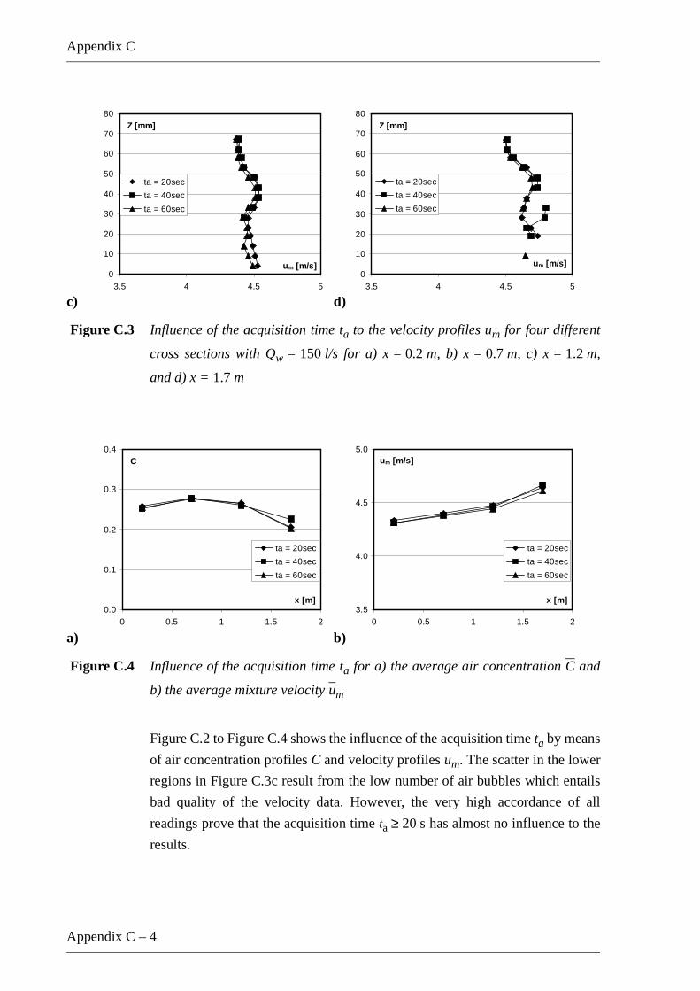
Appendix C
Appendix C – 4
c) d)
Figure C.3 Influence of the acquisition time ta to the velocity profiles um for four different
cross sections with Qw = 150 l/s for a) x = 0.2 m, b) x = 0.7 m, c) x = 1.2 m,
and d) x = 1.7 m
a) b)
Figure C.4 Influence of the acquisition time ta for a) the average air concentration C and
b) the average mixture velocity um
Figure C.2 to Figure C.4 shows the influence of the acquisition time ta by means
of air concentration profiles C and velocity profiles um. The scatter in the lower
regions in Figure C.3c result from the low number of air bubbles which entails
bad quality of the velocity data. However, the very high accordance of all
readings prove that the acquisition time ta ≥ 20 s has almost no influence to the
results.
0
10
20
30
40
50
60
70
80
3.5 4 4.5 5
um [m/s]
Z [mm]
ta = 20sec
ta = 40sec
ta = 60sec
0
10
20
30
40
50
60
70
80
3.5 4 4.5 5
um [m/s]
Z [mm]
ta = 20sec
ta = 40sec
ta = 60sec
0.0
0.1
0.2
0.3
0.4
0 0.5 1 1.5 2
x [m]
C
ta = 20sec
ta = 40sec
ta = 60sec
3.5
4.0
4.5
5.0
0 0.5 1 1.5 2
x [m]
um [m/s]
ta = 20sec
ta = 40sec
ta = 60sec

Development of Aerated Chute Flow
Appendix C – 5
C.3 Influence of channel width
a) b)
c) d)
Figure C.5 Influence of the channel width to the air concentration profiles for four cross
sections with Qw = 150 l/s for a) x = 0.2 m, b) x = 0.7 m, c) x = 1.2 m, and
d) x = 1.7 m
0
10
20
30
40
50
60
70
80
0.0 0.2 0.4 0.6 0.8 1.0
C
Z [mm]
y = 5.0 cm
y = 11.5 cm
y =20.0 cm
y = 30.0 cm
y = 38.5 cm
y = 45.0 cm
0
10
20
30
40
50
60
70
80
0.0 0.2 0.4 0.6 0.8 1.0
C
Z [mm]
y = 5.0 cm
y = 11.5 cm
y =20.0 cm
y = 30.0 cm
y = 38.5 cm
y = 45.0 cm
0
10
20
30
40
50
60
70
80
0.0 0.2 0.4 0.6 0.8 1.0
C
Z [mm]
y = 5.0 cm
y = 11.5 cm
y =20.0 cm
y = 30.0 cm
y = 38.5 cm
y = 45.0 cm
0
10
20
30
40
50
60
70
80
0.0 0.2 0.4 0.6 0.8 1.0
C
Z [mm]
y = 5.0 cm
y = 11.5 cm
y =20.0 cm
y = 30.0 cm
y = 38.5 cm
y = 45.0 cm

Appendix C
Appendix C – 6
a) b)
c) d)
Figure C.6 Influence of the channel width y to the velocity profiles um for four cross
sections with Qw = 150 l/s for a) x = 0.2 m, b) x = 0.7 m, c) x = 1.2 m,
d) x = 1.7 m
0
10
20
30
40
50
60
70
80
0.0 1.0 2.0 3.0 4.0 5.0 6.0
um [m/s]
Z [mm]
y = 5.0 cm
y = 11.5 cm
y =20.0 cm
y = 30.0 cm
y = 38.5 cm
y = 45.0 cm0
10
20
30
40
50
60
70
80
0.0 1.0 2.0 3.0 4.0 5.0 6.0
um [m/s]
Z [mm]
y = 5.0 cm
y = 11.5 cm
y =20.0 cm
y = 30.0 cm
y = 38.5 cm
y = 45.0 cm
0
10
20
30
40
50
60
70
80
0.0 1.0 2.0 3.0 4.0 5.0 6.0
um [m/s]
Z [mm]
y = 5.0 cm
y = 11.5 cm
y =20.0 cm
y = 30.0 cm
y = 38.5 cm
y = 45.0 cm0
10
20
30
40
50
60
70
80
0.0 1.0 2.0 3.0 4.0 5.0 6.0
um [m/s]
Z [mm]
y = 5.0 cm
y = 11.5 cm
y =20.0 cm
y = 30.0 cm
y = 38.5 cm
y = 45.0 cm

Development of Aerated Chute Flow
Appendix C – 7
a) b)
Figure C.7 Influence of the channel width for a) the average air concentration C90, and
b) the average mixture velocity um
Figure C.5 to Figure C.7 show measurements taken over the channel width y by
means of air concentration and velocity profiles. Note that the air concentration
profiles show a higher air concentration on the left side wall (y = 5 cm)
compared to the right side wall (y = 45 cm). This difference can be explained by
the inflow conditions effected by the inflow pipe and the jetbox which level of
after x = 1.7 m due to the high turbulence as shown in Figure C.5d. The velocity
profiles in Figure C.6 show a normal velocity distribution in high turbulent open
channel flow. The channel centre line was not influenced by shock waves from
the side walls.
C.4 Discharge measurements
a) b)
0.0
1.0
2.0
3.0
4.0
5.0
6.0
0 0.5 1 1.5 2
x [m]
um [m/s]
y = 5.0 cm
y = 11.5 cm
y = 20 cm
y = 30 cm
y = 38.5 cm
y = 45.0 cm0.0
0.1
0.2
0.3
0.4
0 0.5 1 1.5 2
x [m]
C90
y = 5.0 cm y = 11.5 cm
y = 20 cm y = 30 cmy = 38.5 cm y = 45.0 cm
0.0
10.0
20.0
30.0
40.0
50.0
60.0
70.0
80.0
0.0 2.0 4.0 6.0
uW [m/s]
Z [mm]
y = 5.0 cm
y =15.0 cm
y = 25.0 cm
y = 35.0 cm
y = 45.0 cm
Mean0.0
10.0
20.0
30.0
40.0
50.0
60.0
70.0
80.0
0.0 2.0 4.0 6.0
uW [m/s]
Z [mm]
y = 5.0 cm
y =15.0 cm
y = 25.0 cm
y = 35.0 cm
y = 45.0 cm
Mean

Appendix C
Appendix C – 8
c) d)
e) f)
Figure C.8 Influence of the channel width y to the water velocity for six measurements with
a) Qw = 150 l/s, x = 0.2 m, b) Qw = 150 l/s, x = 0.7 m,
c) Qw = 200 l/s, x = 0.2 m, c) Qw = 200 l/s, x = 0.7 m,
e) Qw = 200 l/s, x = 1.2 m, and f) Qw = 200 l/s, x = 1.7 m
0.0
10.0
20.0
30.0
40.0
50.0
60.0
70.0
80.0
90.0
0.0 2.0 4.0 6.0 8.0
uW [m/s]
Z [mm]
y = 5.0 cm
y =15.0 cm
y = 25.0 cm
y = 35.0 cm
y = 45.0 cm
Mean0.0
10.0
20.0
30.0
40.0
50.0
60.0
70.0
80.0
90.0
0.0 2.0 4.0 6.0 8.0
uW [m/s]
Z [mm]
y = 5.0 cm
y =15.0 cm
y = 25.0 cm
y = 35.0 cm
y = 45.0 cm
Mean
0.0
10.0
20.0
30.0
40.0
50.0
60.0
70.0
80.0
90.0
0.0 2.0 4.0 6.0 8.0
uW [m/s]
Z [mm]
y = 5.0 cm
y =15.0 cm
y = 25.0 cm
y = 35.0 cm
y = 45.0 cm
Mean0.0
10.0
20.0
30.0
40.0
50.0
60.0
70.0
80.0
90.0
0.0 2.0 4.0 6.0 8.0
uW [m/s]
Z [mm]
y = 5.0 cm
y =15.0 cm
y = 25.0 cm
y = 35.0 cm
y = 45.0 cm
Mean

Development of Aerated Chute Flow
Appendix C – 9
Figure C.9 Error estimation for water discharge from the measuring system
a) measured discharge Qw with Qw(IDM) = 150 l/s,
b) measured discharge Qw with Qw(IDM) = 200 l/s
Figure C.8 shows the pure water velocity distribution for 5 measurements over
the channel width and the mean velocity at various x-positions for two
discharges Qw = 150 l/s and Qw = 200 l/s for the So = 10 % chute slope.
Integrating the velocity distributions according to equation (3.2) over the flow
depth h and the channel width b, the discharge should result in the discharge
measured from the IDM. Frictional wall effects may be noted in Figure C.8 by
lower velocities for y = 5cm and y = 45 cm compared to the mean velocity.
Figure C.9 shows the deviation between the IDM discharge and the measured
water discharge for a) Qw = 150 l/, and b) Qw = 200 l/s, respectively, wall
effects can also be noted.
0.0
50.0
100.0
150.0
200.0
0 0.25 0.5 0.75 1
x [m]
QW [l/s]
y = 5.0 cm y = 15.0 cm
y = 25.0 cm y = 35.0 cm
y = 45.0 cm mean0.0
50.0
100.0
150.0
200.0
250.0
0 0.5 1 1.5 2
x [m]
Qw [l/s]
y = 5.0 cm y = 15.0 cm
y = 25.0 cm y = 35.0 cm
y = 45.0 cm mean

Appendix C
Appendix C – 10

Development of Aerated Chute Flow
Appendix D – 1
APPENDIX D CHANNEL ROUGHNESS
Table D.1 Calculation of the friction coefficient f and the equilibrium sand roughness
height ks according to the Darcy-Weissbach equation and the universal formula
Table D.1 shows a summary of selected measurements for the channel
roughness calculations according to equations (3.5) and (3.6).
Qw
[l/s]So hucosα
[m]f ks
[mm]
138.1 0.1 0.044 0.0118 0.000062
184.1 0.1 0.053 0.0113 0.000105
215.0 0.1 0.058 0.0111 0.000503
161.1 0.1 0.048 0.0115 0.000304
207.1 0.1 0.057 0.0111 0.000083
70.0 0.1 0.028 0.0131 0.000044
105.1 0.1 0.038 0.0123 0.000145
140.1 0.1 0.044 0.0117 0.000036
175.1 0.1 0.051 0.0113 0.000046
192.6 0.1 0.052 0.0113 0.000695
207.6 0.3 0.044 0.0116 0.000508
208.0 0.3 0.044 0.0111 0.000527
192.6 0.3 0.041 0.0111 0.000115
192.6 0.5 0.034 0.0117 0.000095
average deviation
0.0115 0.000231

Appendix D
Appendix D – 2
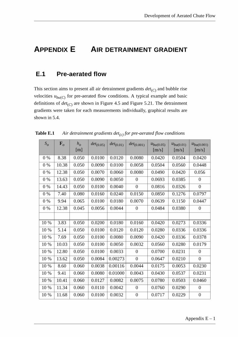
Development of Aerated Chute Flow
Appendix E – 1
APPENDIX E AIR DETRAINMENT GRADIENT
E.1 Pre-aerated flow
This section aims to present all air detrainment gradients det(C) and bubble rise
velocities ubu(C) for pre-aerated flow conditions. A typical example and basic
definitions of det(C) are shown in Figure 4.5 and Figure 5.21. The detrainment
gradients were taken for each measurements individually, graphical results are
shown in 5.4.
Table E.1 Air detrainment gradients det(c) for pre-aerated flow conditions
So Fo ho
[m]det(0.05) det(0.01) det(0.001) ubu(0.05)
[m/s]ubu(0.01)
[m/s]ubu(0.001)
[m/s]
0 % 8.38 0.050 0.0100 0.0120 0.0080 0.0420 0.0504 0.0420
0 % 10.38 0.050 0.0090 0.0100 0.0058 0.0504 0.0560 0.0448
0 % 12.38 0.050 0.0070 0.0060 0.0080 0.0490 0.0420 0.056
0 % 13.63 0.050 0.0090 0.0050 0 0.0693 0.0385 0
0 % 14.43 0.050 0.0100 0.0040 0 0.0816 0.0326 0
0 % 7.40 0.080 0.0160 0.0240 0.0150 0.0850 0.1276 0.0797
0 % 9.94 0.065 0.0100 0.0180 0.0070 0.0639 0.1150 0.0447
0 % 12.38 0.045 0.0056 0.0044 0 0.0484 0.0380 0
10 % 3.83 0.050 0.0200 0.0180 0.0160 0.0420 0.0273 0.0336
10 % 5.14 0.050 0.0100 0.0120 0.0120 0.0280 0.0336 0.0336
10 % 7.69 0.050 0.0100 0.0080 0.0090 0.0420 0.0336 0.0378
10 % 10.03 0.050 0.0100 0.0050 0.0032 0.0560 0.0280 0.0179
10 % 12.80 0.050 0.0100 0.0033 0 0.0700 0.0231 0
10 % 13.62 0.050 0.0084 0.00273 0 0.0647 0.0210 0
10 % 8.60 0.060 0.0038 0.00116 0.0044 0.0175 0.0053 0.0230
10 % 9.41 0.060 0.0080 0.01000 0.0043 0.0430 0.0537 0.0231
10 % 10.41 0.060 0.0127 0.0082 0.0075 0.0780 0.0503 0.0460
10 % 11.34 0.060 0.0110 0.0042 0 0.0760 0.0290 0
10 % 11.68 0.060 0.0100 0.0032 0 0.0717 0.0229 0

Appendix E
Appendix E – 2
10 % 6.50 0.080 0.0160 0.0140 0.0014 0.0720 0.0630 0.0063
10 % 6.50 0.060 0.0133 0.0130 0.0168 0.0518 0.0507 0.0065
10 % 6.50 0.050 0.0100 0.0888 0.0136 0.0356 0.0316 0.0484
10 % 6.50 0.040 0.0110 0.0098 0.0100 0.0318 0.0306 0.0318
10 % 6.50 0.030 0.0250 0.0024 0.0024 0.06889 0.0066 0.0066
30 % 5.11 0.060 0.0074 0.0155 0.0143 0.0227 0.0476 0.0500
30 % 7.71 0.060 0.0120 0.0180 0.0060 0.0552 0.0829 0.0276
30 % 10.28 0.060 0.0088 0.0066 0 0.0540 0.0405 0
30 % 11.53 0.060 0.0091 0.0074 0 0.0698 0.0568 0
30 % 14.12 0.050 0.0046 0 0 0.0354 0 0
30 % 3.99 0.110 0.0130 0.0160 0.0250 0.0405 0.0530 0.0779
30 % 5.14 0.100 0.0130 0.0116 0.0192 0.0515 0.0640 0.0761
30 % 7.60 0.800 0.0120 0.0170 0 0.0638 0.0904 0
30 % 10.19 0.065 0.0100 0.0083 0 0.0639 0.0530 0
50 % 5.11 0.060 0.0078 0.00160 0.0212 0.0239 0.0491 0.0384
50 % 7.71 0.060 0.0100 0.0116 0 0.0460 0.0534 0
50 % 10.28 0.060 0.0087 0.0037 0 0.0534 0.0227 0
50 % 11.53 0.060 0.0085 0 0 0.0575 0 0
50 % 14.12 0.050 0.0039 0 0 0.0300 0 0
50 % 3.93 0.110 0.0012 0.0010 0.0212 0.0362 0.0312 0.0661
50 % 5.14 0.100 0.0140 0.0138 0.0074 0.0555 0.0547 0.0293
50 % 7.60 0.080 0.0120 0.0040 0 0.0638 0.0957 0
50 % 10.19 0.065 0.0095 0.0068 0 0.0607 0.0434 0
So Fo ho
[m]det(0.05) det(0.01) det(0.001) ubu(0.05)
[m/s]ubu(0.01)
[m/s]ubu(0.001)
[m/s]

Development of Aerated Chute Flow
Appendix E – 3
E.2 Aerator flow
This section aims to present all air detrainment gradients det(C) and bubble rise
velocities ubu(C) for aerator flow.
Table E.2 Air detrainment gradients det(c) for aerator flow conditions
So Fo ho
[m]det(0.05) det(0.01) det(0.001) ubu(0.05)
[m/s]ubu(0.01)
[m/s]ubu(0.001)
[m/s]
0 % 6 0.050 0.0450 0.0400 0.0260 0.1891 0.1681 0.1093
0 % 8 0.050 0.0600 0.0150 0.0180 0.3362 0.0840 0.1009
0 % 9.9 0.050 0.0600 0.0100 0.0100 0.4202 0.0700 0.0700
0 % 11 0.050 0.0700 0.0085 0.0120 0.5393 0.0655 0.0924
0 % 11.65 0.050 0.0870 0.0070 0.0020 0.7098 0.0571 0.0163
0 % 6 0.080 0.0800 0.0250 0.0180 0.4252 0.1329 0.0957
0 % 8 0.065 0.0800 0.0180 0.0140 0.5111 0.1150 0.0894
0 % 13 0.045 0.0100 0.0070 0.0030 0.0864 0.0605 0.0259
10 % 4 0.050 0.0650 0.0300 0.0240 0.1821 0.0840 0.0672
10 % 6 0.050 0.0650 0.0420 0.0170 0.2731 0.1765 0.0714
10 % 8 0.070 0.0323 0.0158 0.0167 0.2141 0.1047 0.1107
10 % 8 0.050 0.0400 0.0160 0.0025 0.2241 0.0896 0.0140
10 % 9.7 0.050 0.0400 0.0130 0.0030 0.2801 0.0910 0.0210
10 % 11 0.050 0.0220 0.0095 0.0068 0.1516 0.0655 0.0469
10 % 6 0.060 0.0500 0.0270 0.0170 0.2302 0.1243 0.0783
10 % 7 0.060 0.0560 0.0270 0.0140 0.3007 0.1450 0.0752
10 % 8 0.060 0.0290 0.0110 0.0093 0.01780 0.0675 0.0571
10 % 9 0.060 0.0260 0.0100 0.0088 0.1795 0.0690 0.0608
10 % 9.74 0.060 0.0367 0.0100 0 0.2742 0.0747 0
30 % 4 0.060 0.0200 0.0136 0.0166 0.0675 0.0417 0.0509
30 % 6 0.060 0.0272 0.0124 0.0040 0.1252 0.0571 0.0184
30 % 8 0.060 0.02802 0.110 0 0.1719 0.0675 0
30 % 9.43 0.060 0.0400 0.0062 0 0.2894 0.0449 0
30 % 11 0.050 0.0300 0.0041 0 0.2311 0.0316 0
30 % 3 0.110 0.0610 0.0330 0.0150 0.1901 0.1028 0.0467
30 % 4 0.100 0.332 0.0214 0.0110 0.1315 0.0848 0.0436
30 % 6 0.800 0.0430 0.0160 0.0030 0.2286 0.0850 0.0159

Appendix E
Appendix E – 4
30 % 8 0.065 0.0380 0.0087 0 0.2428 0.0556 0
50 % 4 0.060 0.0228 0.0168 0.0011 0.0700 0.516 0.0035
50 % 6 0.060 0.0370 0.0137 0 0.1703 0.0631 0
50 % 8 0.060 0.0260 0.0040 0 0.1596 0.0246 0
50 % 9.04 0.060 0.0350 0.0010 0 0.2427 0.0069 0
50 % 11 0.050 0.0168 0 0 0.1294 0 0
50 % 3 0.110 0.0390 0.0190 0.0190 0.1215 0.0592 0.0592
50 % 4 0.100 0.0320 0.0180 0.0010 0.1268 0.0713 0.0040
50 % 6 0.080 0.0410 0.0170 0 0.2286 0.0948 0
50 % 8 0.065 0.0038 0.0010 0 0.0243 0.0064 0
So Fo ho
[m]det(0.05) det(0.01) det(0.001) ubu(0.05)
[m/s]ubu(0.01)
[m/s]ubu(0.001)
[m/s]

Development of Aerated Chute Flow
Appendix F – 1
APPENDIX F SUMMARY OF MEASUREMENTS
F.1 Overview
All measurements conducted in this project are summarised in Table F.1 and
Table F.2.
Table F.1 Summary of the pre-aerated measurements
So Fo ho
[m]air supply
systemQw
[l/s]Qa
[l/s]comment
0 % 8.38 0.050 pre-aeration 105.1 41.6 variing inflow
Froude number Fo
with constant inflow
depth ho
0 % 10.38 0.050 pre-aeration 140.1 41.6
0 % 12.38 0.050 pre-aeration 175.1 41.6
0 % 13.63 0.050 pre-aeration 192.6 46.1
0 % 14.43 0.050 pre-aeration 204.0 48.6
0 % 7.40 0.080 pre-aeration 212.6 43.3 variing inflow
Froude number Fo
and variing inflow
depth ho
0 % 9.94 0.065 pre-aeration 207.6 50.4
0 % 16.13 0.045 pre-aeration 194.4 46.8
0 % 14.38 0.045 no air supply 215.0 0
10 % 3.83 0.050 pre-aeration 52.5 14.5 variing inflow
Froude number Fo
with constant inflow
depth ho
10 % 5.14 0.050 pre-aeration 70.0 20.0
10 % 7.69 0.050 pre-aeration 105.1 29.5
10 % 10.03 0.050 pre-aeration 140.1 38.6
10 % 12.80 0.050 pre-aeration 175.1 49.1
10 % 13.62 0.050 pre-aeration 192.6 45.8
10 % 8.60 0.060 pre-aeration 138.1 59.9 variing inflow
Froude number Fo
with constant inflow
depth ho
10 % 9.41 0.060 pre-aeration 161.1 55.5
10 % 10.41 0.060 pre-aeration 184.1 55.51
10 % 11.34 0.060 pre-aeration 207.1 53.9
10 % 11.68 0.060 pre-aeration 215.0 53.9

Appendix F
Appendix F – 2
10 % 6.50 0.080 pre-aeration 180.0 49.4 model families to
investigate the
critical scaling flow
depth
10 % 6.50 0.060 pre-aeration 116.9 33.5
10 % 6.50 0.050 pre-aeration 88.9 24.5
10 % 6.50 0.040 pre-aeration 63.6 17.8
10 % 6.50 0.030 pre-aeration 41.3 11.7
30 % 5.11 0.060 pre-aeration 92.1 25.4 variing inflow
Froude number Fo
with constant inflow
depth ho
30 % 7.71 0.060 pre-aeration 138.1 39.3
30 % 10.28 0.060 pre-aeration 184.1 52.4
30 % 11.53 0.060 pre-aeration 208.0 57.3
30 % 14.12 0.050 pre-aeration 192.6 54.7
30 % 3.99 0.110 pre-aeration 171.4 56.7 variing inflow
Froude number Fo
and variing inflow
depth ho
30 % 5.14 0.100 pre-aeration 198.1 56.7
30 % 7.60 0.800 pre-aeration 212.6 56.8
30 % 10.19 0.065 pre-aeration 207.6 56.8
50 % 5.11 0.060 pre-aeration 92.1 25.4 variing inflow
Froude number Fo
with constant inflow
depth ho
50 % 7.71 0.060 pre-aeration 138.1 39.2
50 % 10.28 0.060 pre-aeration 184.1 52.4
50 % 11.53 0.060 pre-aeration 203.1 56.0
50 % 14.12 0.050 pre-aeration 192.6 54.9
50 % 3.93 0.110 pre-aeration 171.4 57.1 variing inflow
Froude number Fo
and variing inflow
depth ho
50 % 5.14 0.100 pre-aeration 198.1 57.1
50 % 7.60 0.080 pre-aeration 212.6 56.4
50 % 10.19 0.065 pre-aeration 207.6 56.3
50 % 4.00 0.060 no air supply 92.1 0 variing inflow
Froude number Fo
with constant inflow
depth ho
50 % 6.00 0.060 no air supply 138.1 0
50 % 8.00 0.060 no air supply 184.1 0
50 % 9.32 0.060 no air supply 214.5 0
50 % 11.00 0.050 no air supply 192.6 0
So Fo ho
[m]air supply
systemQw
[l/s]Qa
[l/s]comment

Development of Aerated Chute Flow
Appendix F – 3
Table F.2 Summary of the aerator measurements
50 % 3.00 0.110 no air supply 171.4 0 variing inflow
Froude number Fo
and variing inflow
depth ho
50 % 4.00 0.100 no air supply 198.1 0
50 % 6.00 0.080 no air supply 212.6 0
50 % 8.00 0.065 no air supply 207.6 0
So Fo ho
[m]air supply
systemQw
[l/s]Qa
[l/s]comment
0 % 6.00 0.050 aerator 105.1 21.5 variing inflow
Froude number Fo
with constant inflow
depth ho
0 % 8.00 0.050 aerator 140.1 28.9
0 % 10.00 0.050 aerator 175.1 35.5
0 % 11.00 0.050 aerator 192.6 39.2
0 % 11.65 0.050 aerator 204.0 42.2
0 % 6.00 0.080 aerator 212.6 43.3 variing inflow
Froude number Fo
and variing inflow
depth ho
0 % 8.00 0.065 aerator 207.6 42.46
0 % 11.65 0.050 aerator 204.0 42.30
0 % 13.00 0.045 aerator 194.4 41.15
0 % 11.65 0.050 aerator 212.6 43.3 no additional air
supply
10 % 3.00 0.050 aerator 52.5 14.4 variing inflow
Froude number Fo
with constant inflow
depth ho
10 % 4.00 0.050 aerator 70.0 20.0
10 % 6.00 0.050 aerator 105.1 29.7
10 % 8.00 0.050 aerator 140.1 38.8
10 % 8.00 0.070 aerator 232.0 48.15
10 % 10.00 0.050 aerator 175.1 19.4
10 % 6.00 0.060 aerator 138.1 49.62 variing inflow
Froude number Fo
with constant inflow
depth ho
10 % 7.00 0.060 aerator 161.1 49.89
10 % 8.00 0.060 aerator 184.1 49.6
10 % 9.00 0.060 aerator 207.1 49.6
10 % 9.74 0.050 aerator 224.2 49.6
So Fo ho
[m]air supply
systemQw
[l/s]Qa
[l/s]comment

Appendix F
Appendix F – 4
30 % 4.00 0.060 aerator 92.1 25.2 variing inflow
Froude number Fo
with constant inflow
depth ho
30 % 6.00 0.060 aerator 138.1 38.6
30 % 8.00 0.060 aerator 184.1 49.3
30 % 9.43 0.060 aerator 217.0 48.5
30 % 11.00 0.050 aerator 192.6 49.5
30 % 3.00 0.110 aerator 171.4 47.7 variing inflow
Froude number Fo
and variing inflow
depth ho
30 % 4.00 0.100 aerator 198.1 47.8
30 % 7.60 0.800 aerator 212.6 48.0
30 % 8.00 0.065 aerator 207.6 48.0
30 % 6.00 0.060 aerator 138.1 0.40 no additional air
supply30 % 8.00 0.060 aerator 184.1 0.53
30 % 9.47 0.060 aerator 218.0 0.63
50 % 4.00 0.060 aerator 92.1 25.7 variing inflow
Froude number Fo
with constant inflow
depth ho
50 % 6.00 0.060 aerator 138.1 39.7
50 % 8.00 0.060 aerator 184.1 47.6
50 % 9.43 0.060 aerator 217.0 49.6
50 % 11.00 0.050 aerator 192.6 50.5
50 % 3.00 0.110 aerator 171.4 49.0 variing inflow
Froude number Fo
and variing inflow
depth ho
50 % 4.00 0.100 aerator 198.1 50.5
50 % 6.00 0.080 aerator 212.6 49.3
50 % 8.00 0.065 aerator 207.6 47.4
50 % 4.00 0.060 no air supply 92.1 0 variing inflow
Froude number Fo
with constant inflow
depth ho
50 % 6.00 0.060 no air supply 138.1 0
50 % 8.00 0.060 no air supply 184.1 0
50 % 9.38 0.060 no air supply 216.0 0
50 % 11.00 0.050 no air supply 192.6 0
50 % 3.00 0.110 no air supply 171.4 0 variing inflow
Froude number Fo
and variing inflow
depth ho
50 % 4.00 0.100 no air supply 198.1 0
50 % 6.00 0.080 no air supply 212.6 0
50 % 8.00 0.065 no air supply 207.6 0
So Fo ho
[m]air supply
systemQw
[l/s]Qa
[l/s]comment

Development of Aerated Chute Flow
Appendix F – 5
F.2 Data CD
All conducted data are separated for each measurement. They are structured on
the Data CD into the four chute slopes So, the air supply system (aerator or
pre-aeration) and the inflow Froude number Fo, further in:
inflow[1•1]
local[19•35]
streamwise[19•1]
uniform[1•1]
inflow height
ho [m]
local air concentra-
tion C
average air concentration
C90
average uniform air concentration
C90u
inflow air discharge Qa [l/s]
streamwise coordinate
x [m]
bottom air concentration
Cb
uniform mixture flow depthh90u [m]
inflow water dischargeQw [l/s]
vertical coordinate
z [m]
mixture flow depth
h90 [m]
inflow Reynolds number
Ro
water depthhw [m]
inflow Weber number
Wo

Appendix F
Appendix F – 6
The Data CD is available on request at
Email: [email protected]
URL: http://www.vaw.ethz.ch/