Department of Electronic Systems Antennas Propagation and Radio Networking

Mobile Communication

Fredrik Bajers Vej 7A1 · Aalborg University · DK - 9220 Aalborg · Denmark

Title : “Small antennas on dielectric materials for 4G applications”

Project period:

10th Semester

Student : Lorenzo Maccarrone

Supervisors: Samantha Caporal Del BarrioMauro PelosiGert F. Pedersen

Number of pages:Delivered: June,1st 2011

1

Abstract:

Nowadays, antenna size reduction

represents a crucial point in the design of a

mobile device. Until now, several works has

been done with a focus on different

techniques that face this challenge.

Specifically, the effect of a high-permittivity

ceramic dielectric substrate on the antenna

size was analyzed. In order to investigate

this aspect and to design the antenna in the

UMTS band, simulations was done using the

FDTD method. In this thesis it has been

shown, that at a fixed resonant frequency,

the antenna size and its bandwidth depend on

the value of permittivity dielectric substrate.

Using the higher dielectric substrate, it is

possible to reduce the radiator size but, it is

accompanied by a reduction in bandwidth.

Then, the antenna is smaller and narrowband

for high permittivity values. The antenna

behavior is described in terms of bandwidth,

quality factor, efficiency and mismatch loss.

2

The content of this report is freely available, but publication (with reference source) may only be pursued due toagreement with the respective authors

Preface

This report has been written as a project for the 10t h semester final master thesis within the ambit of

Erasmus study project between University of Catania and Aalborg University, specifically between

Department of Telecommunication at Catania University and Department of Electronic Systems

at Aalborg University , during the period February2011 – June 2011

A correct interpretation of the following report is possible referring to a list of literature references,

that are marked in square brackets , a list of equations, that are marked in brackets, and also all

chapters are numerated, as shown in table of contents.

Report Structure

This report is about “ Small antennas on the dielectric materials for 4G applications”.

This is divided in the following parts:

- Five numbered chapters, with a description of the project arguments.

-The appendices which are arranged alphabetically.

3

Table of contents

Abstract……………………………………………………………………………………………1

Preface……………………………………………………………………………………………..3

Report structure…………………………………………………………………………………..3

Table of Contents…………………………………………………………………………………4

List of Symbols……………………………………………………………………………………6

Chapter 1:Introduction

1.1 - Evolution of Mobile System Standards…………………………………………..…9

1.2 - LTE systems…………………………………………………………………….…..11

1.3 - MIMO systems……………………………………………………………….……..12

1.4 - Problem Definition………………………………………………………………….14

1.5 - Simulation environment……………………………………………………………14

Chapter 2 : Technical Background

2.1 - Main Antennas Parameters …………………………………………………………15

2.2 - Field regions………………………………………………………………………….15

2.3 – Radiation Patterns…………………………………………………….……………16

2.4 - Radiation Power density…………………………………………….………………..17

2.5 - Radiation intensity…………………………………………………….……………18

2.6 – Directivity…………………………………………………………….…………….18

2.7 - Antenna impedance and reflection coefficient…………………….……………….19

4

2.8 - Accepted power and mismatch loss…………………………………………………21

2.9 - Antenna radiation efficiency………………………………………………………..22

2.10 – Gain…………………………………………………………………………………..22

2.11 – Bandwidth…………………………………………………………………………..23

2.12 - Quality factor………………………………………………………….……………24

Chapter 3 : Small antennas for handset

3.1 - Planar inverted folded antenna (PIFA)……………………………..…………….25

3.1.1- PIFA with meandering. Design and simulation results………………..29

3.1.2- PIFA dual band. Design and simulation results………………………..31

3.2 – FICA. . Design and simulation results ………………………………..…………32

Chapter 4 : Small antennas with ceramic material

4.1 - State of the art ceramics…………………………………………………………..34

4.2 - High dielectric substrate…………………………………………………….…….35

4.3 - Small antenna with dielectric substrate…………………………………………..36

4.4 - Reduction size……………………………………………………………………..37

4.5 - Simulation and results…………………………………………………..………..38

4.6 - Quality factor……………………………………………………………………..42

Chapter 5 : Conclusions

5.1Conclusions…………………………………………………………………………46

Reference………………………………………………………………..……………………47

5

Appendix A : Matlab scripts……………………………………………………………..49

List of symbols

ε electric permittivity

ε r electric relative permittivity

ε 0 permeability in free space

σ electric conductivity

μ magnetic permeability

μ0 permeability in free space

ρ density

Г voltage reflection coefficient

ω angular frequency

λ wavelength

k free space wave number

c speed of light in free space

β bandwidth

Δx x-directed space increment

Δy y-directed space increment

Δz z-directed space increment

Δt unit time step

E⃗ electric field

6

H⃗ magnetic field

D⃗ electric flux density

B⃗ magnetic flux density

J⃗ electric current density

M⃗ magnetic current density

D directivity

A⃗ , F⃗ potential vectors

e0 antenna efficiency

ed dielectric efficiency

er reflection efficiency

ecd radiation efficiency

f frequency

f r resonant frequency

G gain

G|¿|¿ absolute gain

PA accepted power

Pavailable total available power from the source

Ploss power consumed in the load or the imperfect conductor

Prad total radiated power

Q quality factor

Qlb low band quality factor

RA antenna resistance

7

Rr radiation resistance

Rg generator resistance

Rl loss resistance

S11 return loss

U radiation intensity

vp numerical phase velocity

L1 length of the antenna patch

L2 width of the antenna patch

H height between the ground plane and antenna radiating element

W width of the short cut element of antenna

X A antenna reactance

X g generator reactance

ZA antenna inpedance

Z¿ input impedance

Z0 characteristic impedance

8

Chapter 1: Introduction

The 4 Generation Mobile Communication systems are projected to provide a wide variety of

new services, like high quality voice, high definition video, high data rate wireless channels. It

include also several types of broadband wireless access communication systems. It support mobile

service and fixed wireless networks.

The goal of 4G systems might be synthesized with the word - Integration.

The following part of this chapter is an overview of evolution of mobile systems, highlighting the

aspects and characteristics of the LTE systems, and the benefits of MIMO technology.

1.1-Evolution of Mobile System Standards To reach the current 4G mobile systems has been a long process. The history and evolution

of mobile service from 1Genaration to 4 Generation are mentioned briefly in this section. The

earliest service were implemented in 1970s, based on basic cellular structure of mobile

communication and analog technology. In the beginning, the phones adopted analog radio channels

(frequencies around 450 MHz), used for voice calls only, and their signals transmitted by the

method of frequency modulation (FM). This kind of phones had some disadvantages, such as a poor

security due to the lack of encryption. Furthermore, numerous incompatible analog systems were

placed in service around the world during the 1980s.

The most prominent 1G systems was Advanced Mobile Phone System (AMPS), that was the

first 1G system to start operating in the USA (in July 1978), Nordic Mobile Telephone (NMT),

and Total Access Communication System (TACS).

With the 2-Generation systems, instead, networks radio signals were digital encrypted technology.

Moreover, 2G used digital multiple access technology, such as TDMA and FDMA, were

significantly more efficient over their predecessors.

These 2G systems was provided circuit-switched data communication services at a low speed and

SMS text messages services.

The continuous evolution of design and implement digital systems led to a variety of different

standards such as GSM, Cordless Telephone, DECT, and PACS.

9

During the 1990s, 3G mobile system was defined and was relatively to be adopted, with the aim to

eliminate previous incompatibilities and become a really global system.

I this way, the 3G systems had higher quality voice channels, as well as broadband data capabilities,

up to 2 Mbps. Unfortunately, their differences could not reconciled, with the consequent adoption

of two mobile standards for 3G. The 2.5G was an interim step between 2G and 3G. It was basically

an enhancement of the two major 2G technologies to provide increased capacity on the 2G radio

frequency channels and to introduce higher throughput for data service, up to 384 kbps. A very

important aspect of 2.5G was that the data channels were optimized for packet data, with

consequently introducing access to the Internet from mobile devices, whether telephone, Personal

Digital Assistant (PDA), or Laptop. This generation ,still used in some country, offers extended

features, it has additional capacity on the 2G systems, such as GPRS, EDGE, HSCSD. Furthermore,

it offers wireless multimedia IP-based services and applications.

The protocol used in 3G systems support high speeds and are targeted for other applications apart

from voice, such as motion video, mp3, video conferencing and fast Internet access.

UMTS system is one of the 3G mobile telecommunications systems. There are many radio

spectrum frequencies designated for the operation of the UMTS. In this project, we consider only

the frequencies for band I, II, V, XIV, which are showed in the following table.

Operating Band

Frequency Band

Commond name

Uplink Downlink Region

I 2100 IMT 1920-1980 2110-2170 Europe, Asia, Korea, Japan, New Zealand , Brazil

II 1900 PCS 1850-1910 1930-1990 North America

V 850 CLR 824-849 869-894 North America, Australia, New Zealand, Brazil

XIV 700 SMH 788-798 758-768 America (future)

Table1. UMTS Bands

10

1.2 - LTE Systems

LTE (Long Term Evolution) or 3G Long Term Evolution is the evolution of mobile cellular

communications technology towards broadband IP network. The aim of the 3GPP project is to

further develop the Universal Mobile Telecommunications System (UMTS) standard and moreover

provide an enhanced and simplified technology on mobile broadband. The main keys of the 4G

infrastructures are accessing information anywhere, anytime, with a seamless connection to a wide

range of information and services, and receiving a large volume of information, data, video,

pictures.

With 4G, a range of new services and models are available to provide a comprehensive and secure

all IP solution to laptop, smart phones and other handset devices. The requirements for this

standards are peek speed at 100 Mbit/s for high mobility and 1Gbit/s for low mobility [1] .

The 4G infrastructures consist of a set of various networks using IP (Internet protocol) as a common

protocol so that users are in control because they are able to choose every application and

environment. Based on the developing trends of mobile wireless communication, 4G has broader

bandwidth, higher data rate, and smoother and quicker handoff, all that to ensure service across a

multitude of wireless systems and networks.

The performance of radio communications depends on an antenna system, termed smart or

intelligent antenna. Recently, multiple antenna technologies are emerging to achieve the goal of 4G

systems. In this sense, the spatial multiplexing technology and the MIMO technology gained

importance for its bandwidth conservation and power efficiency. In fact, spatial multiplexing

involves deploying multiple antennas at the transmitter side and at the receiver side. Independent

streams can then be transmitted simultaneously from all the antennas. The usage of the MIMO

technology multiplies the base data rate by the number of transmit antennas or the number of

receive antennas. Apart from this, the reliability in transmitting high speed data in the fading

channel, with the TX – RX diversity, can be improved by using more antennas at the transmitter or

at the receiver. Both transmit-receive diversity and transmit spatial multiplexing are categorized

into the space-time coding techniques, which does not necessarily require the channel knowledge at

11

the transmitter. The other category is closed-loop multiple antenna technologies, which require

channel knowledge at the transmitter.

1.3 - MIMO SystemsMIMO is an acronym that means Multiple-Input Multiple-Output [2]. In fact, several

transmitters and receivers can be used at each end of the radio link in order to achieve a high

capacity. The signal multiplexing is used for MIMO between multiple transmitting antennas (space

multiplex) and frequency or time. This technology uses the OFDM for the channel access. The

signal transmitted by m antennas is received by n antennas. Processing of the received signals may

deliver several performance improvements in terms of range, quality of received signal and

spectrum efficiency. In principle, MIMO is more efficient when many multiple path signals are

received, as shown the 802.11n standard, the theoretical speed upper than 600 Mbit/s. However, the

performance in cellular deployments is still subject to research and simulations. Moreover, it is

generally admitted that the gain in spectrum efficiency is directly related to the minimum number of

antennas in the link.

Figure 1 shown various MIMO configurations [3] , for example:

Figure1. Radio access channel, variations of MIMO

12

MIMO: Several antennas are placed at the transmitter and receiver.

MISO: Several antennas are placed in the transmitter but only one in the receiver.

SIMO: Only one antenna is placed in the transmitter and several are located in the receiver.

SISO: Only one antenna is placed in both the transmitter and the receiver.

The main requirement for MIMO systems is that the antennas must be able to receive different

signals, even though if they are closely spaced. The different signal paths should be uncorrelated

to ensure a good diversity gain and the mutual coupling has to be as less as possible to avoid

the energy transfer between antennas and therefore, the increase of the correlation.

Due to this requirements, implement MIMO systems in mobile phone is nowadays still a challenge,

because it is difficult to add multiple antennas on something so small and pretend to have

a good isolation. Another feature is that the performance of the antenna will be degraded by the

effects of inter-antenna coupling, envelope cross-correlation and coupling to biological tissues in

the user’s hands.

Some advantage of MIMO technology [3] are :

- Array gain, that increase in received SNR (Signal Noise Rate), like a results from a coherent

combining effect of the wireless signals at a receiver. The coherent combining could be

realized through spatial processing at the receive antenna and/or spatial pre-processing at the

transmit antenna.

- Spatial diversity gain, that mitigates fading and it is realized by providing the receiver with

multiple transmitted signals in space, frequency or time. With an increasing number of

independent multiple copies of the same signal, the probability that at least one of the copies

is not experiencing a deep fade increases, then improving the quality and reliability of

reception.

- Spatial multiplexing gain, that offers a linear increasing in data rate, transmitting multiple and

independent data streams within the bandwidth of operation. Moreover, the spatial

multiplexing gain increases the capacity of a wireless network.

- Interference reduction, that in general results from multiple users sharing time and frequency

resources. This kind of interference may be mitigated by exploiting the spatial dimension to

increase the separation between users. Furthermore, the spatial dimension can be leveraged 13

for the purposes of interference avoidance minimizing interference to other users.

Interference reduction and avoidance improve range and coverage of a wireless network.

In general, it may not be possible to reach simultaneously all the benefits described because

to conflicting demands on the spatial degrees of freedom. Nevertheless, the usage of some

combination of this across a wireless network could be to improve capacity, reliability , and

coverage.

1.3 – Problem definition

The antenna size reduction of a mobile device is nowadays a crucial point of a designer. Until now,

studies are largely focused on different techniques able to doing this. However, it has been shown

the effects of a high-permittivity ceramic dielectric substrate on the size of an antenna.

This thesis focuses on the design of an antenna in UMTS band, using the FDTD method. The size

of that is reduced depending on the value of permittivity and keeping the same resonant frequency.

It is shown the bandwidth is also reduced and therefore, the antenna is narrowband. The antenna

behavior is described in terms of bandwidth, quality factor, efficiency, losses and mismatch loss.

1.4 - Simulation Enviorement

It was used the AAU3 software to make all the simulations of this thesis. The code was

written in Matlab high-level. This software allows to design antenna and to generate, using the

FDTD method, the main output parameters in electro- magnetic, for example the radiation

patterns, smith chart, impedance, radiation, efficiency. There are two types of running the

simulations: either by Matlab kernel or by Fortran FDTD kernel, which is fastercompared in the

compilation duration.

The finite difference time domain (FDTD) computational algorithm is used to give a solution of

the Maxwell’s equations, it is based on the Yee’s algorithm. Contrary to Moment Method, this

method gives a straightforward solution of the six-coupled field components of the Maxwell’s

curl equations. The electric and the magnetic field components are computed [17] “by

discretizing the Maxwell’s curl equations both in time and space, and then solving the

discretized equations in a time marching sequence by alternatively calculating the electric and

magnetic fields in the computational domain”.

14

Chapter 2: Technical Background

2.1 - Main antennas parameters

To describe how antennas irradiate energy and build them to optimize its performance, it is

necessary to introduce the following parameters and the most important electrical properties.

The performance of an antenna can be evaluated through the input impedance, the gain, the

mismatch and absorption [4] .

2.2 - Field regions

It is usually to subdivide the space surrounding an antenna into three regions [4] :

- the reactive near field, that is the region immediately surrounding the antenna;

- the Fresnel region, or radiating near field zone, that is between the other two regions

- the Fraunhofer region ,or far field zone, that it is calculated according the Rayleigh

condition.

Figure shown the three different zone, note that they depend on the distance R from the

antenna surface, the largest dimension D of an antenna and the wavelength λ.

15

Figure 2.1 : field zone of an antenna

2.3 – Radiation Patterns

An antenna pattern is defined in as [4] : “a mathematical function or a graphical

representation of radiation properties of the antenna as a function of space coordinates.

In most case, the radiation pattern is described in the far-field region and is represented

as a function of the directional coordinates. Radiation properties include power flux

density, field intensity, radiation intensity, field strength directivity, polarization or

phase ”.

16

Figure 2.2: (a) radiation lobes of an antenna pattern. (b) linear plot of power pattern.

In general, it is a good instrument to evaluate the behavior of an antenna, specifically the

radiation lobes and power pattern.

2.4 - Radiation Power density

An electromagnetic field is used to transport information through a communication

medium, wireless or guiding structure, from one point to the other. Energy and power

are associated with electromagnetic wave. In this sense, the Poynting vector, that is a

power density, is defined as [4]:

W⃗ = E⃗*H⃗

17

with :

W⃗ is the instantaneous Poynting vector (W/m2)

E⃗ is the instantaneous electric field intensity (V/m)

H⃗ , instantaneous magnetic field intensity (A/m)

However, the instantaneous total power P (W) crossing a closed surface may be

obtained by integrating the normal component, over the entire surface, of the

Poynting vector. That in equation form is :

P⃗ =∮W⃗ ·ds⃗

However, the time average Poynting vector may be calculated using the equation [4] :

W av= 12 Re(E⃗ · H⃗ ¿)

Where:

W av = average power density (W/m2)

The average power radiated is defined as:

Pav = Prad= ∮W⃗ rad·ds⃗ = = 12∮ℜ( E⃗ · H⃗ ¿)·ds⃗

Therefore, the power pattern of an antenna is defined as a function of direction, of

average power density radiated.

2.5 - Radiation intensity

The Radiation intensity in a given direction is defined as: “ power radiated from an

antenna per unit solid angle” [4] and is calculated [4] as:

U = r2 W rad

Where:

18

U is the radiation intensity (W/unit solid angle)

W rad is the radiation density (W/m2)

2.6 – Directivity

The directivity is defined [4] as: “the ratio of the radiation intensity in a given

direction from the antenna to the radiation intensity averaged over all directions. The

average radiation intensity is equal to the total power radiated by the antenna divided

4 π ”, and it is calculated [4] as:

D = UU 0

=4 πUP rad

Where :

U is the radiation intensity

U 0 is the radiation intensity of isotropic source

both evaluated in (W/ unit solid angle)

Prad is the total radiated power (W)

Therefore, the radiation intensity for maximum directivity is:

Dmax= D0 = Umax

U 0 =

4 π Umax

Prad

Where :

D is the directivity

D0 is the maximum directivity

Umax is the maximum radiation intensity

19

U 0 is the radiation intensity of isotropic source

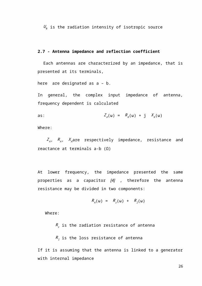
2.7 - Antenna impedance and reflection coefficient

Each antennas are characterized by an impedance, that is presented at its terminals,

here are designated as a – b.

In general, the complex input impedance of antenna, frequency dependent is calculated

as: ZA(ω) = RA(ω) + j X A(ω)

Where:

ZA, RA, X Aare respectively impedance, resistance and reactance at terminals a-b (Ω)

At lower frequency, the impedance presented the same properties as a capacitor [4] ,

therefore the antenna resistance may be divided in two components:

RA(ω) = Rr(ω) + Rl(ω)

Where:

Rr is the radiation resistance of antenna

Rl is the loss resistance of antenna

If it is assuming that the antenna is linked to a generator with internal impedance

ZG(ω) = Rg(ω) + j X g(ω)

Where:

Zg is generator internal impedance (Ω)

Rg is resistance of generator impedance (Ω)

X g is reactance of generator impedance (Ω)

Consequently, the maximum power delivered to the antenna are presented when :

20

Rr+ Rl = Rg

X A=−Xg

The following figure shown an antenna coupled to the generator, in terms of equivalent

circuit, when the transmission mode is used :

Figure 2.3 (a)Antenna model , (b) (c) equivalent circuit

Note: for this part, it is assuming that quarter wave antenna exhibits a nominal 50 ohm

characteristic impedance.

Instead, the reflection coefficient of the antenna is [bal]:

Г = Z¿−Z0

Z¿+Z0

21

Where :

Z¿ is the input impedance of the antenna;

Z0 is the characteristic impedance of the source and the feedline,

according that the feedline is matched to the source ;

2.8 - Accepted power and mismatch loss

Considering that the accepted power (AP) is defined as the power delivered to the

antenna terminal from source, its depends by reflection coefficient:

AP = (1 - ׀ Г ׀ 2)P¿

Where :

AP is the accepted power

P¿ is the input power

Instead, the corresponding mismatch loss to the accepted power is defined as:

APP¿

׀ – 1 = Г ׀ 2

And the mismatch in dB is:

ML(dB) = -10 log(1 – ׀ Г ׀ 2)

2.9 - Antenna radiation efficiency

There are in literature several methods to calculate the radiation efficiency, for

example the pattern integration method, Q- factor method and Wheller method, such as

is illustrated in [D], some of these making the calculation easier.

22

The radiation efficiency erad is the amount of power that propagates far field from the

power delivered to the terminals of antenna. Can be written as [4] :

erad = P rad

AP = AP - Pdiss

Pdiss is the dissipated power in the antenna;

Generally, all the possible losses can be taken into account through total efficiency e t,

that may be written as [5] or [4]:

e t= er ec ed = P rad

P¿

Where the quantity are dimension-less:

er is the reflection (mismatch)efficiency,

ec is the conduction efficiency

ed is the dielectric efficiency

In this way it is possible to consider the losses due to reflection, conduction and

dielectric losses;

2.10 - Gain

The gain describes an important way to evaluate the performance of an antenna. It is

function of the efficiency and the directional capability. A gain definition is given in [4]

as : ” the ratio of the intensity, in a given direction, to the radiation intensity that would

be obtained if the power accepted by the antenna were radiated isotropically. The

radiation intensity corresponding to the isotropically radiated power is equal to the

power accepted by the antenna divided 4𝜋 ”. That corresponds as:

Gain = 4 𝜋 UP¿

Where :23

U is the radiation intensity

Furthermore, when the antenna is perfectly matched, that means Z¿ = ZC,

The gain may be related to the total efficiency and the directivity in the following way:

Gain = e t· D

Where D is the directivity.

2.11 - Bandwidth

The bandwidth , noted as BW, is defined as [4] : “the range of frequencies within

which the performance of the antenna, with respect to some characteristic, conforms to

a specified standard”.

In general, for a mobile handset antenna, the objective is a bandwidth that covering the

operative frequency bands. Using this parameter it is possible to evaluate if an antenna is

broadband or narrowband, This dimensions often depends the antenna size and

mismatch effect . In this work, it is considered for a handset antenna that the limit is S11

= -6 dB at the border of the frequency band , that corresponds to a power reflection of

25 %, as explained in [6] .

2.12 - Quality factor

The quality factor is described in function of small antennas property and of

bandwidth. There are some method to define the quality factor, some of these are

considered following. It represents a parameter giving a well indication on the

bandwidth. Indeed, it is evaluate for a tuned antenna at the resonating frequency f 0 .

According to [4] , is defined :” the tuned antenna is one whose feed point reactance is

tuned to zero at a frequency f 0 using a single, lossless, series tuning element having a

reactance X s(ω0) = −X A (ω0) “.

A way to define the quality factor is:

Q(ω0) = ω0 W (ω0)

P¿(ω0)

24

Where:

ω0is the tuned frequency;

W (ω0) is the internal energy;

P¿(ω0) is the power accepted;

It is possible to approximate the exact value of the quality factor as:

Q ¿) ≈ Q z¿) = ω0

2 RA (ω0) √RA' ( ω0 )2+(X A

' (ω0 )+⃒ X A (ω0) ⃒

ω0) ²

It is possible to define a relation for bandwidth and quality factor that is suitable for all

frequency range. As is written in [4] : “The definition of bandwidth suitable for this

purpose is fractional matched VSWR bandwidth, FBRW V (ω0 ) ,where the VSWR of the

tuned antenna is determined using a characteristic impedance, equal to the antenna’s

feed point resistance”.

The fractional matched VSWR bandwidth is defined as [7] :

FBW V (ω0 )=ωH−ωL

ω0 = Δf

f 0 ∝ 1

Q

Moreover, It is possible to relate the Fractional matched VSWR bandwidth and Q as [7]:

Q (ω0 )≈ Q z¿) = 2√β

FBW V ( ω0 ) , √ β = s−12√ s

≤1

Or more simply, the Q factor may be written in according to [8] :

Q ¿) = ω2 RA (ω)

dX A (ω )dω

Chapter 3 : Small antennas for handset

25

In general, the antennas are designed and measured in well-defined environments,

on both ground planes of infinite or large. However, in a small electrical device such as handset

communication terminals, the antenna will undergo a distortion of its radiation characteristics.

Therefore, it is therefore important to emphasize that the integration of an antenna in a terminal is

very complex, therefore the design of a portable antenna is not an easy task and certainly will affect

the actual behavior with regard to both the input and radiation characteristics [1, 2].

However, this type of antenna is subject to very strict specifications [3]. Small, compact, light

weight, low profile, strength and flexibility are the main considerations taken into account in

conventional small antenna design [4]. To this we must add, as new mobile devices are required to

operate to different standards, their antennas are expected to grab as much spectrum as possible, so

they can cover multi-band and broadband [5].

Although the development in microelectronics led to a more significant reduction in the size of the

terminal, the size of the antenna cannot be so simply reduced, due to physical factors. Indeed, this

could bring restrictions on the polarization, the radiation efficiency and bandwidth, and also

increases the sensitivity to manufacturing tolerances. In the past, some compromises have been

taken in relation to performance the antenna, and the deterioration in some of its performance

characteristics has been accepted, whether the objectives of integration and cost were achieved.

However, in recent years the trend is changing, and network operators wishing to obtain terminals

even more efficient.

The highly efficient proposed 4G technologies will certainly make use of MIMO technologies to

further reduce interference and provide for extra capacity require in future applications. However,

this require multiple antennas at ends of downlink and uplink. The current trend on the reduction of

volume of mobile devices leads to a consequent reduction in the size of the antenna, but at the same

time be able to operate on a larger number of frequency bands, corresponding to its number of

diverse wireless systems a portable device. Miniaturization, integration, multi-band operation, and

the final performances were instrumental in choosing the design of initial models.

Considering that an antenna that covers continuously without tuning a wide spread of frequency

bands is a single-band but also wideband antenna. But, today’s wireless terminology, an antenna

that operates double bands frequencies, like GSM 900 and GSM1800 frequencies is considered a

multi-band antennas.

Tree different antenna models are shown in this chapter. The first two are a PIFA model and the last

one is a FICA model, which exhibit respectively single and multiband behavior. 26

3.1 - Planar Inverted Folded Antenna

This section provide a description of the characteristics of the planar inverted –F antenna , that is a

more popular antenna for portable wireless devices because of its low profile, small size, and built-

in structure [9].

The other major advantages are easy fabrication, low manufacturing cost, and simple structure [10].

Also, PIFA’s inherent bandwidth is higher than the bandwidth of the conventional patch antenna,

because since a thick air substrate is used.

The basic PIFA, with a grounded patch antenna at λ/4 and patch length instead of λ/2, formed by a

top element of a radiating patch , a ground plane which is fed from a transmission line between a

DC shorting plate .Moreover, are considered some variations of dual-band or multi-band PIFAs

suitable for application in mobile units reported recently [11],[12],[13],[14].

In the Figure 3.1 it shows the geometry of a conventional single band PIFA element. Modifying

these ones, leaves the possibility to design well adapted antennas following different handset

bandwidth [10].

Figure 3.1 : PIFA model

A major advantage concerning the PIFA is that the dimension of the patch can be reduced,

introducing the short circuit element between the feed and the ground plane. In addition, using a

shorting element of a smaller dimension than that of the patch, the effective inductance of the

antenna increases and the resonant frequency becomes lower. In fact, to have a PIFA resonating at a

low band frequency, the current distribution effective length has to be as long as possible. To take

27

advantage of the longest length of the patch, the ratio between the length (L1) and the width (L2) of

the patch, has to be as high as possible, with a shorting element small behind the dimension of the

edge [15].

In other terms,

L₁L₂

≥ 1 ,W ≪ L₁

The fundamental step that has to be done when designing a new PIFA is the calculation of the patch

dimension to make the antenna resonate at the right frequency. At first, the formula relying on the

plate dimensions with the wavelength was the following:

L₁+L₂ =λ4 ❑

⇔f r =

c4 (L₁+L ₂)

Nevertheless, it does not consider the presence of the shorting plate, which gives :

L₁+H =λ4 ❑

⇔f r₁ =

c4 (L₁+H ) , for

WL₁=1

or

L₁+L₂+H =λ4 ❑

⇔f r₂ =

c4 (L₁+L ₂+H) , for W=0

and

L₁+L₂+H - W=λ4

⇔

f r2 =

c4 (L1+L2+H −W ) , for 0<

WL₁<1

Where:

f r: Resonance frequency [Hz]

c: Vacuum light speed 3·108,

L₁: Length of the PIFA antenna[m]

L₂: Width of the PIFA antenna [m]

H: height between the ground plane and the patch

28

W : the width of the shorting element

Consequently, it is understandable that the resonant frequency is increasing with the width of the

plate because of the negative sign at the denominator before W. As it is explained in [15], the

resonant frequency , when 0 < WL₁< 1, can be approximated thanks to the following equations :

fr= r·f1+(1-r)·f2, for L1L2 > 1

And

fr =rk ·f1+(1-rk), forL1L2>1

with r = WL₁ and K= L1

L2 .

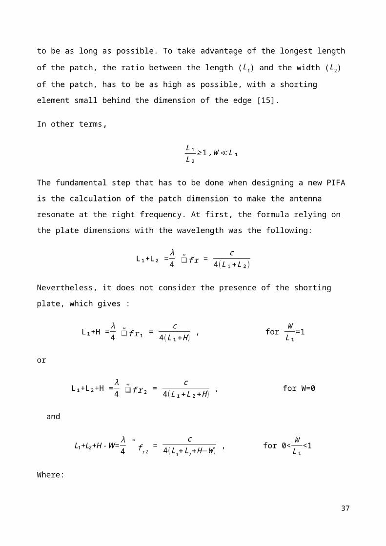
The mismatch loss is rising with the growth of the L₁/L ₂ ratio whereas; the bandwidth is going

down linearly.

Figure 3.2 (a) Bandwidth of the PIFA when short circuit plate width is equal L1[15]

29

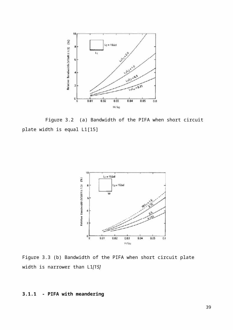
Figure 3.3 (b) Bandwidth of the PIFA when short circuit plate width is narrower than L1[15]

3.1.1 - PIFA with meandering

The first model investigated was a single band PIFA antenna. The design is showed in Figure 3.4.

The geometry of the proposed structure along with definition of its dimensions. The antenna design

proposed is showing the matching property at 796 MHz . The dimensions of the plate is fixed at

40x20 mm .The width of the ground plane is kept fixed at 40 x 100 mm to cover the whole part of

the patch. The meandering are long 210 mm and width is 1 mm. The distance between patch and

ground plan is 5 mm. The distance between source and short is 4 mm.

Figure 3.4 PIFA design1

30

During the simulation, it shown that changing the distance between source and short, can give

mismatch of coupling and gain loss. Such as, the bandwidth is increasing when the patch and the

ground plane are getting closer each other. Moving the short away from the feeding source shows

that both the bandwidth and frequency resonance are modified. Indeed, the most far is the short

away from the source, and the higher is the resonant frequency.

As shown in Figure 3.5, the maximum return loss is -31.28 dB at 796 MHz. The upper and lower

band frequencies are 778 MHz and 813 MHz, respectively, giving the absolute bandwidth of 35

MHz. Therefore, the bandwidth obtained for the proposed PIFA is 4.4%.

Figure 3.5 PIFA design1. S11 parameter

Figure 3.6 shows the smith chart, and describes the matching obtained in the simulation, where the

colored part is interest frequency range.

Figure 3.6: Smith chart

31

3.1.2– PIFA Dual band

This PIFA model exhibits two resonant mode, obtained on the same patch volume. The geometry of

the proposed structure is shown in Fig. 3.7 ( note: the ground plane is not showed ) along with

definition of its dimensions. The original conception of this kind if antenna is showed in [19].The

antenna design proposed is showing the matching property both at 772 MHz and 1942 MHz . The

dimensions of the plate is fixed at 40x24 mm .The width of the ground plane is kept fixed at 40 x

100 mm to cover the whole part of the patch. The distance between patch and ground plan is h=5

mm.

Figure 3. PIFA design2

This design of antenna exhibits two resonating in UMTS band. The first is in band XIV, its

presents the S11 equal to -21.93 dB at 774 MHz and the bandwidth is narrowband, only 15 MHz.

The second frequency range is in band I, that presents the S11 equal to -14,94 at 1942 MHz, and

bandwidth is 70 MHz .A great matching is achieved with the between source and short equal to d =

3 mm.

Figure 3.8 S11 parameters

3.2 - FICA32

According to [18], the Folded Inverted Conformal Antenna is a kind of antennas that exhibits three

resonating modes, which operate by sharing the same antenna volume. The geometry of the

proposed structure is shown in Fig. 3.9 along with definition of its dimensions. The dimensions of

the plate is fixed at 40x24 mm .The width of the ground plane is kept fixed at 40 x 100 mm to cover

the whole part of the patch. The distance between patch and ground plan in this case is different, it

is equal to h = 5 mm.

Figure 3.9 FICA antenna

How shown in the following figure 3.10, this design exhibits the I - II - V UMTS bands

Figure3.10 FICA. S11 parameters

33

It is shown in the Smith chart, that the antenna has greater matching property at 850 MHz

Figure 3.11 FICA Smith chart

Moreover, it is possible to allow a spreading of the reactive electromagnetic energy in all the

antenna volume with this configuration [19]. In this way, the antenna exhibits a lower Q factor and

produces a wider radiating bandwidth.

34

Chapter 4

Small antennas with ceramic material

4.1 - State of the art ceramics

The demand for smaller, cheaper antennas are increased because of higher integration with the

packaging structures of mobile device systems. Many methods have been proposed and explored in

achieving miniaturization of antennas.[22-28]. For example, a shorting wall has been used to

decrease the size by a factor two[22]. Orting posts near the feed have taken this a step

further[23,24]. Another approach for antenna size reduction is to employ substrate[25].

The use of ceramic materials, that presents high dielectric constant and low loss, it is a new

approach to reducing the antenna size. This types of antenna are called Ceramic chip antenna, made

by a ceramic substrate block and metal patterns printed on it. Some studies done on antenna types

have shown that it is possible to use high constant ceramic substrate allowing a good antenna

reduction size.

For instance, using a substrate with constant of 20, resulting an area of only 25%, compared to

using an FR4 substrate. Otherwise, an antenna on ceramic with two different permittivity dielectric

value, the fist one is the Barium - Titanate with a dielectric constant of 37 and the second ones is

neodymium-titanate substrates with a dielectric constant of 85. In the first case, the operating

frequency was 1,5 GHz, used a BaTiO3 substrate with ε r =37, the area of the antenna was 333 mm.

The second case was with a Neodymium -Titanate substrate withε r =85,the area of the antenna area

was 105,16 mm, with a possible reduction size of more than 85% over a conventional antenna on

FR4 substrate. It is considered a thickness equal to 2.54 and, in the best case, the bandwidth was

only 2.5 MHz . According to [34], to get a reasonable small antenna on a 2 mm thick substrate, with

high dielectric constant 38, the antenna reduction dimension is significantly smaller then 1/10 of the

wavelength, and the bandwidth is only 4,72 MHz .

4.1 - High dielectric ceramics substrate

A number of works in the literature have reported or calculated results on the effects of high

permittivity [33].There are several types of ceramic materials, each of these having different

thermal stables properties, that depends on the frequency use[32]. What emerges from state of the

35

art , most of the materials using a higher permittivity, i.e greater than 80, are mixed with low other

dielectric material on texture[35], combining both the its benefits. In addition, synthetic dielectric

can be produced by mixing materials of two or more different dielectric constants. This types of

substrate lead to texture substrate. These types of substrates lead to textured substrates, which

provide for additional design control, useful in impedance matching. Combining all of these

characteristics with a broadband (bowtie) antenna design, it is possible to improve upon past

benchmarks of efficiency and bandwidth while maintaining significant miniaturization. As is well

known, increasing the dielectric constant of the antenna substrate (while reducing the dimensions of

the device) results in narrower bandwidths [20].

With the use a dielectric substrate with large permittivity and overall size reduction at fixed

operating frequency, the impedance bandwidth of antenna is usually decreased. Figure shows the

effect of substrate thickness on impedance bandwidth and efficiency for two values of dielectric

constants [24]. While the bandwidth increases monotonically with thickness, a decrease in the value

ε rvalue increases the bandwidth.

Figure4.1 Effect of substrate thickness on impedance

bandwidth and efficiency for two dielectric constants

36

4.3 - Small antenna with dielectric substrate

Because the Fyrkat didn't work for several days in the last month, now it is possible to present in

this project only results on the FICA antenna model, choice due because of its lower quality factor

and broadband characteristics.

As a result of the sensitivity analysis, all of simulations in this section are settled as follows:

Fc[MHz] Fs[MHz] Time[s] PML thickness

[cells]

Number of time steps

Cella size Energy computed

[step]1500 2300 1x10−9 8 100000 0,0005 100

Figure 4.2 the FDTD parameters used in the simulations

In this section, all the antenna model are designed to resonate around at a theoretical frequency of

850 MHz .

Figure4.3 FICA model reduced. ε r = 20

37

According to the commercial furniture of the ceramic substrate and the appropriate value of their

tangent loss value, the conductivity values have been calculate for different frequency values. It was

used the following formulas:

σ= ε 0 εrωtgd

frequency Tang loss εr=1 εr=4 εr=16 εr=20

845 Mhz 0,001 4.65*10^-5 1.86*10^-4 7.44*10^-4 9.3*10^-4

0,005 2.32*10^-4 9.4*10^-4 3.76*10^-3 4,7*10^-30,01 4.65*10^-4 1.86*10^-3 7.44*10^-3 9.3*10^-3

0.02 9.3*10^-4 3.76*10^-3 1.5*10^-2 1.18*10^-2795 Mhz 0,01 4.41*10^-4 1.76*10^-3 7.05*10^-3 8.82*10^-3

1950 Mhz 0,01 1.08*10^-3 4.34*10^-3 1.735*10^-2 2.17*10^-2

Figure 4.4 Conductivity values

4.4 - Reduction size

The antenna design with a high dielectric value allows a reduction antenna size

Antenna_Type

Frequency Substrate [ε r]

Area[mm²]

Miniaturization by a factor size

Bandwidth [MHz]

Q efficiency

FICA 845 air 960 - 118 7.1 1.00

847 4 377 2,54 17,12 49.47

0.98

852 16 155 6,19 9.17 92 0.74845 20 135 7,1 7.6 110 0.60

Figure 4.5 Reduction size

38

4.5 - Simulation and results

It is shown a result loss comparison between different permittivity value.

Figure 4.6 Return loss comparison between different value of ε r, band I -V

Figure Return loss comparison between different value of ε r, band V

Increasing the permittivity value, the antenna became narrowband.

39

Figure4.7 Return loss comparison between different

value of tangent loss. ε r =4

Figure 4.8 Return loss comparison between different value of

tangent loss. Band V ε r =4

40

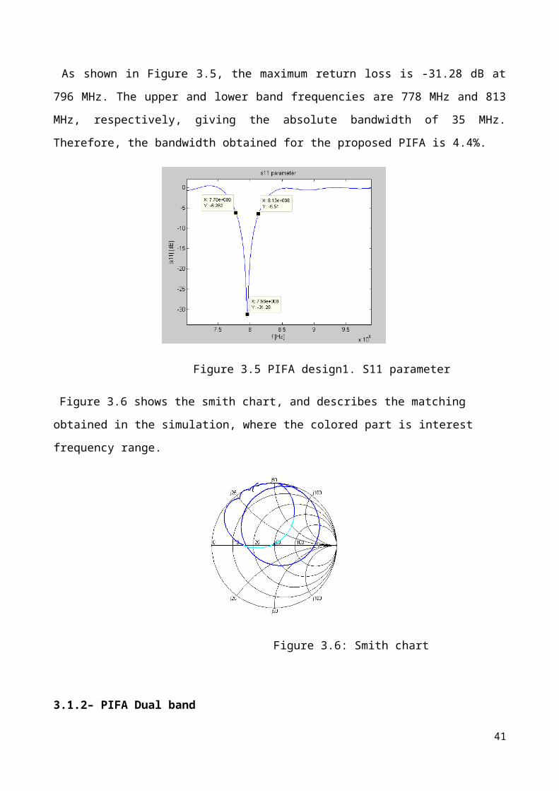
Figure 4.9 S11dB BI, BV. ε r =16

Figure 4.10 Return loss comparison between different value of

tangent loss. Band V. ε r =16

41

Figure 4.11 Return loss comparison between different value of

tangent loss. Bands I-V ε r =20

Figure 4.12 Return loss comparison between different value of

tangent loss BV. ε r =20

42

4.6 - Quality factor

It is possible to evaluate the quality factor of an multiband antenna according to [37]

Figure 4.13 FICA model. Comparison of exact Quality factor

Figure 4.14 FICA ε r =4. Comparison of exact Quality factor

43

Figure 4.15 FICA ε r =4. Comparison of the quality factor

for different values of tangent loss

This figure showed that increasing the tangent loss value, the quality is reduced.

Figure 4.16 FICA ε r =16. Comparison of exact Quality factor

44

Figure 4.17 FICA ε r =20. Comparison of exact Quality factor

Figure 4.18 FICA ε r =4 . Mismatch loss for different values of tangent loss

45

Figure 4.19 FICA ε r =16 . Mismatch loss for different values of tangent loss

Figure 4.20 FICA ε r = 20. Mismatch loss for different values of tangent loss

This means that the mismatch loss is increased when the tangent loss value is increased

46

Chapter 5 Conclusion

The goal of this project has been achieved partially. In effect, a resize of a antenna FICA has been

done, using high permittivity value of 20 has been achieved a reduction factor of 20 with only 7.6

MHZ of bandwidth . Instead, a minimal bandwidth of 20 MHz has been almost possible using

dielectric constant of 4 and a miniaturization by a factor size of 2,4. It has shown that the bandwidth

is inversely proportional to the quality factor.

Therefore, the optimal choice of an antenna that has a low quality factor is critical for this type of

investigation.

Moreover, as said to increase the bandwidth could change the thickness of the substrate.

More simulations have been done about the FICA antenna design, for example has been increased

the thickness of the substrate, but that choice has made it difficult to strictly design of all antennas

at different values of permittivity.

Also, it will be possible evaluate the performances of ceramic antennas when

when other components are placed in close proximity.

Furthermore, it will be important investigate the human hand influence on the small antenna

performance

47

Reference[1] ITU global standard for international mobile telecommunications ´IMT-Advanced´

[2] http://www.ieee.li/pdf/viewgraphs/wireless_mimo.pdf

[3] A. Constantinides A. Goldsmith A. PaulRaj H. Vincent Poor E. Biglieri, R. Calderbank.

MIMO Wireless Communications. Cambridge University Press, 2007

[4] C. Balanis : “Antenna Theory - Analysis and Design, Third Edition”

[5]. Kazuhiro Hirasawa, Misao Haneishi. “Analysis, Design, and Measurement of Small and Low-Profile Antennas”.

1992.

[6]. F. Gustrau, D. Manteuffel. “EM Modeling of Antennas and RF Components for Wireless Communication Systems”.

2006.

[7]. Impedance, Bandwidth, and Q of Antennas. Best, Arthur D. Yaghjian and Steven R. 2005.

[8]. Antennas, from Theory to Practice. Yi Huang, Kevin Boyle. 2008.

[9]F. Wang, Z. Du, Q. Wang and K. Gong, “Enhanced-bandwidth PIFA with T-shaped ground plane”, Electronic Letters,

vol. 40, no. 23, pp. 1504 – 1505, Nov. 2004.

[10 ]B. Kim, J. Hoon and H. Choi, “Small wideband PIFA for mobile phones at 1800 MHz,” Vehicular Technology

Conference, vol.-1, pp. 27-29, May 2004.

[11] Z. D. Liu, P. S. Hall, and D. Wake, “Dual-frequency planar F antenna,” IEEE Trans. Antennas Propagation., vol. 45,

pp. 1451-1458, Oct. 1997.

[12] C. R. Rowell and R. D. Murch, “A compact PIFA suitable for dual-frequency 900/1800-MHz operation,” IEEE Trans.

Antennas Fropagat., vol. 46, pp. 596-598, April 1998.

[13] S. Tarvas and A. Isohatala, “An internal dual-band mobile phone antenna,” in 2000 IEEE Antennas Propagat.

Soc. mt. Symp. Dig., pp. 266-269.

[14] C. T. P. Song, P. S. Hall, H. Ghafouri-Shiraz, and D. Wake, “Triple band planar inverted F antennas for

handheld devices,” Electron. Lett., vol. 36, pp. 112-1 14, Jan. 20, 2000.

[15] Kazuhiro Hirasawa, Misao Haneishi. “Analysis, Design, and Measurement of Small and Low-Profile Antennas”.

1992.

[15] Mittra, R., and S. Dey, “Challenges in PCS Antenna Design,” IEEE Antennas and

Propagation Society International Symposium Digest, 1999, pp. 544–547.

[16] D. M. Pozar and D. H. Schaubert, Microstrip Antennas:,the Analysis and Design of Microstrip Antennas and Arrays, New York: IEEE Press, 1995.

48

[17] A. Taflove, “Computational electrodynamics: the finite-difference time-domain method”Artech House 1995 first edition

[18] C. Di Nallo, A. Faraone, “Multiband internal antennas for mobile phones”. Electronics letters vol41.

[19] Vainikainen,P.,:” Resonator-based]analysis of the combination of mobile handset antenna and chassis”, IEEE

Trans. Antenna Propag. 2002,50(10),pp.1433-1444.

[20] “ Multiband Antenna for GSM and 3G Mobile System”. ABDURAHMAN M M OWAG. 2006

[21] B. Lee and F.J. Harackiewiez, “Miniature Microstrip Antenna with a Partially filled High Permittivity Substrate”, IEEE Transactions on Antenna and Propagation, AP-50, August 2002 pp 1160-1162[22]. S. Pinhas and S. Shtrikman, "Comparison Between Computed and Measured Bandwidth of Quarter-

Wave Microstrip Radiators," IEEE Transactions on Antennas and Propagation, AP-36, November

1988, pp. 1615-1616.

[23]. R. B. Waterhouse, "Small Microstrip Patch Antenna," Electronics Letters, 31, April 1995, pp. 604-605.

[24]. Y. J. Wang, C. K. Lee, W. J. Koh, and Y. B. Gan, "Design of Small and Broad-Band Internal Antennas for IMT-

2000 Mobile Handsets," IEEE Transactions on Microwave Theory Techniques, MTT-49, August 200 1, pp. 1398-1403.

[25]. T. K. Lo, C.-O. Ho, Y. Hwang, E. K. W. Lam, and B. Lee, "Miniature Aperture-Coupled Microstrip Antenna of

Very High Permnittivity," Electronics Letters, 33, January 1997, pp. 9-10.

[26]. K.-L. Wong and K.-P. Yang, "Small Dual-Frequency Microstrip Antenna with a Cross Slot," Electronics

Letters, 33, November 1997, pp. 1916-1917.

[27]. K.-L. Wong and K.-P. Yang, "Modified Planar Inverted F Antenna," Electronics Letters, 34, January 1998, pp. 7-8.

[28]. B. Lee and F. J. Harackiewicz, "Miniature Microstrip Antenna with a Partially Filled High-Permittivity

Substrate," IEEE Transactions on Antennas and Propagation, AP-50, August 2002, pp. 1160-1162.

[29]. D. R. Jackson and N. G. Alexopoulos, "Simple Approximate Formulas for Input Resistance, Bandwidth, and

Efficiency of a Resonant Rectangular Patch IEEE Transactions on Antennas and Propagation, AP-39, March 199 1,

pp. 407-410.

[30]. E. Chang, S. A. Long, and W. F. Richards, "An Experimental Investigation of Electrically Thick Rectangular

Microstrip Antennas," IEEE Transactions on Antennas and Propagation, AP-34, June 1986, pp. 767-772.

[31].Ahmad Hoorfar and Alessandro Perrotta”An Experimental Study of Microstrip Antennas on Very High

Permittivity Ceramic Substrates and Very Small Ground Planes

[32]. G. Kiziltas, D. Psychoudakis, J. L. Volakis, and N. Kikuchi, "Topology Design Optimization of Dielectric

Substrates for Bandwidth Improvement of a Patch Antenna," IEEE Transactions on Antennas and

Propagation, AP-51, October 2003, pp. 2732- 2743.

[33] D. H. Schaubert and K. S. Yngvesson, “Experimental study of a microstrip array on high permittivity substrate,”

IEEE Trans. Antennas Propagat., vol. AP-34, pp. 92–97, Jan. 1986.

[34] Hans Add, Rainer Wansch and Christoph Schmidt “Antennas for a Body Area Network”

[35] KuW’, D. Pryehoudaltir’, C-C. Ched, L. Vola, H. Halloran, ’ Patch Antenna Miniaturization Using Thick Truncated

Textured Ceramic Substrate

49

[36] D. M. Pozar and D. H. Schaubert, Microstrip Antennas: the Analysis and Design of Micrtostrip Antennas and

Arrays, New York: IEEE Press, 1995.

[37] Arthur D. Yaghjian, Fellow, IEEE, and Steven R. Best, Senior Member, IEEE ,Impedance, Bandwidth,

and Q of Antennas

Appendix A

Matlab scripts

- QUALITY FACTOR

clear all;close all;load prova1_20_002;load prova2_16_002;Rs=50;f0=845;Df=1e6;figure;%in relazione alla formula (81) di pag 1308 del paper:" Impedance, Bandwidth, and Q of Antennas". Qf=abs(((imZ(2:end)'-imZ(1:end-1)').*f_axis(2:end)')/(4.*Df.*Rs)); % imZ, f_axis portati sotto forma di vettore riga plot(f_axis(600:1000),Qf(600:1000));%plot(f_axis,Qf);q=Qf(f0);BW=f0/q;save Q_er20tg002 Qf;

- QUALITY FACTOR L-MATCH

clear all;close all;load prova10_20;load prova1_20;f0=845;Rs=50;ZL=Z_disp(f0);X12=lmatch(Rs,ZL,'r');X12(1,2);X12(2,2);Z1=X12(1,1);if abs(X12(1,2))>abs(X12(2,2)) Z2=j*X12(2,2);else Z2=j*X12(1,2);end X2=(X12(1,2)); X1=(X12(2,2)); if X12(1,2)>0 & X12(2,2)<0

50

C=1/j*2*pi*f_axis*X2; L=X1/j*2*pi*f_axis; %Zin=real(Z_disp)+(j*2*pi*f_axis*L)+(1./(j*2*pi*f_axis*C));else L=X2/j*2*pi*f_axis; C=1/j*2*pi*f_axis*X2; %Zin=real(Z_disp)+(j*2*pi*f_axis*L)+(1./(j*2*pi*f_axis*C));end%Q=50*square(C/L);%Zin= real(Z_disp)+(j*2*pi*C)+1./(j*2*pi*L);Zin=((Z1*(Z2+real(Z_disp)))./(Z1+Z2+real(Z_disp)));gamma=abs((Zin-real(Z_disp))./(Zin+real(Z_disp)));%fprintf('\nBW equal %g MHz,QF equal %g at fr %d MHz\n',BW,Q,f0);plot(f_axis(650:1200),Zin(650:1200),'r')qu20=abs(Zin(f0))load Q_er20 ;hold onplot(f_axis(650:1200),Qf(650:1200),'b')BW20=f0./qu20save BW_20 BW20;save qu_20 qu20

- TWO METHODS QUALITY FACTOR

clear all;close all;load prova10_20;load prova1_20;f0=845;Rs=50;ZL=Z_disp(f0);X12=lmatch(Rs,ZL,'r');X12(1,2);X12(2,2);Z1=X12(1,1);if abs(X12(1,2))>abs(X12(2,2)) Z2=j*X12(2,2);else Z2=j*X12(1,2);end X2=(X12(1,2)); X1=(X12(2,2)); if X12(1,2)>0 & X12(2,2)<0 C=1/j*2*pi*f_axis*X2; L=X1/j*2*pi*f_axis; %Zin=real(Z_disp)+(j*2*pi*f_axis*L)+(1./(j*2*pi*f_axis*C));else L=X2/j*2*pi*f_axis; C=1/j*2*pi*f_axis*X2; %Zin=real(Z_disp)+(j*2*pi*f_axis*L)+(1./(j*2*pi*f_axis*C));end%Q=50*square(C/L);%Zin= real(Z_disp)+(j*2*pi*C)+1./(j*2*pi*L);Zin=((Z1*(Z2+real(Z_disp)))./(Z1+Z2+real(Z_disp)));gamma=abs((Zin-real(Z_disp))./(Zin+real(Z_disp)));%fprintf('\nBW equal %g MHz,QF equal %g at fr %d MHz\n',BW,Q,f0);plot(f_axis(650:1200),Zin(650:1200),'r')qu20=abs(Zin(f0))load Q_er20 ;hold onplot(f_axis(650:1200),Qf(650:1200),'b')BW20=f0./qu20

51

save BW_20 BW20;save qu_20 qu20

-FIND F0 AND BANDWIDTH

clear all;close all;load prova3;load prova1; A=s11db;A=logical(A<-7);B=diff(A);C=find(B>0);%start;D=find(B<0);%endf1=C(1);f2=D(1);f3=C(2);f4=D(2);f5=C(3);f6=D(3); n=size(s11db);i=0; % index of array ekementsv=s11db;% find minmin=v(1);posmin=1;for i=2:nif(v(i)<min)min=v(i);posmin=i;f01=posmin;endendQ1=f01./(f2-f1)fprintf('\nS11db equal %g, at frequency %d MHz\n',min,posmin);

-RESIZE HAND

clear all;close all;%A=rand(5,4,2);load hand6;A=VolArray;%[I,J]=size(A);%[I,J,K]=size(A);[I,J,K]=size(A); %AA=double(zeros(I*2,J*2));AA=double(zeros(I+2,J*2,K*2)); for i=1:I; for j=1:J; for k=1:K; %AA(2*i-1, 2*j-1) =A(i,j); AA(2*i-1, 2*j-1, 2*k-1)=A(i,j,k); endend

52

end for i=1:I; % AA(2*i,:)=AA(2*i-1,:); AA(2*i,:,:)=AA(2*i-1,:,:); end for j=1:J; %AA(:,2*j)=AA(:,2*j-1); AA(:,2*j,:)=AA(:,2*j-1,:); end for k=1:K; AA(:,:,2*k)=AA(:,:,2*k-1); end VolArray=AA;clear A;clear AA;clear I;clear J;clear K;clear i;clear j;clear k;save hand6

- DOUBLE HAND

clear all;close all;%A=rand(5,4,2);load hand1;A=VolArray;%[I,J]=size(A);%[I,J,K]=size(A);[I,J,K]=size(A); %AA=double(zeros(I*2,J*2));AA=double(zeros(I+2,J*2,K*2)); for i=1:I; for j=1:J; for k=1:K; %AA(2*i-1, 2*j-1) =A(i,j); AA(2*i-1, 2*j-1, 2*k-1)=A(i,j,k); endendend for i=1:I; % AA(2*i,:)=AA(2*i-1,:); AA(2*i,:,:)=AA(2*i-1,:,:); end for j=1:J; %AA(:,2*j)=AA(:,2*j-1); AA(:,2*j,:)=AA(:,2*j-1,:); end for k=1:K; AA(:,:,2*k)=AA(:,:,2*k-1); end VolArray=AA;clear A;clear AA;clear I;clear J;clear K;clear i;clear j;

53

clear k;save hand1

54