Embed Size (px)
Citation preview
Comments?E-mail your comments about Synopsys documentation to [email protected]
VCS® MXUser GuideVCS MX X-2005.06August 2005
ii
Copyright Notice and Proprietary InformationCopyright © 2004 Synopsys, Inc. All rights reserved. This software and documentation contain confidential and proprietary information that is the property of Synopsys, Inc. The software and documentation are furnished under a license agreement and may be used or copied only in accordance with the terms of the license agreement. No part of the software and documentation may be reproduced, transmitted, or translated, in any form or by any means, electronic, mechanical, manual, optical, or otherwise, without prior written permission of Synopsys, Inc., or as expressly provided by the license agreement.
Right to Copy DocumentationThe license agreement with Synopsys permits licensee to make copies of the documentation for its internal use only. Each copy shall include all copyrights, trademarks, service marks, and proprietary rights notices, if any. Licensee must assign sequential numbers to all copies. These copies shall contain the following legend on the cover page:
“This document is duplicated with the permission of Synopsys, Inc., for the exclusive use of __________________________________________ and its employees. This is copy number __________.”
Destination Control StatementAll technical data contained in this publication is subject to the export control laws of the United States of America. Disclosure to nationals of other countries contrary to United States law is prohibited. It is the reader’s responsibility to determine the applicable regulations and to comply with them.
DisclaimerSYNOPSYS, INC., AND ITS LICENSORS MAKE NO WARRANTY OF ANY KIND, EXPRESS OR IMPLIED, WITH REGARD TO THIS MATERIAL, INCLUDING, BUT NOT LIMITED TO, THE IMPLIED WARRANTIES OF MERCHANTABILITY AND FITNESS FOR A PARTICULAR PURPOSE.
Registered Trademarks, Trademarks, and Service Marks of Synopsys, Inc.
Registered Trademarks (®)Synopsys, AMPS, Arcadia, C Level Design, C2HDL, C2V, C2VHDL, CoCentric, COSSAP, CSim, DelayMill, DesignPower, DesignSource, DesignWare, Eaglei, EPIC, Formality, in-Sync, LEDA, ModelAccess, ModelTools, PathBlazer, PathMill, PowerArc, PowerMill, PrimeTime, RailMill, RapidScript, SmartLogic, SNUG, Solv-It, SolvNet, Stream Driven Simulator, Superlog, System Compiler, TestBench Manager, TetraMAX, TimeMill, VCS, and VERA are registered trademarks of Synopsys, Inc.
Trademarks (™)BCView, Behavioral Compiler, BOA, BRT, Cedar, ClockTree Compiler, DC Expert, DC Expert Plus, DC Professional, DC Ultra, DC Ultra Plus, Design Advisor, Design Analyzer, Design Compiler, DesignTime, DFT Compiler SoCBIST, Direct RTL, Direct Silicon Access, DW8051, DWPCI, ECL Compiler, ECO Compiler, ExpressModel, Floorplan Manager, FormalVera, FoundryModel, FPGA Compiler II, FPGA Express, Frame Compiler, HDL Advisor, HDL Compiler, Integrator, Interactive Waveform Viewer, JVXtreme, Liberty, Library Compiler, ModelSource, Module Compiler, MS-3200, MS-3400, NanoSim, OpenVera, Physical Compiler, Power Compiler, PowerCODE, PowerGate, ProFPGA, Protocol Compiler, RoadRunner, Route Compiler, RTL Analyzer, Schematic Compiler, Scirocco, Scirocco-i, Shadow Debugger, SmartLicense, SmartModel Library, Source-Level Design, SWIFT, Synopsys EagleV, Test Compiler, TestGen, TetraMAX TenX, TimeTracker, Timing Annotator, Trace-On-Demand, TymeWare, , VCS Express, VCSi, VHDL Compiler, VHDL System Simulator, VirSim, and VMC are trademarks of Synopsys, Inc.
Service Marks (SM)DesignSphere, SVP Café, and TAP-in are service marks of Synopsys, Inc.
SystemCTM is a trademark of Open SystemC Initiative and is used under license. All other product or company names may be trademarks of their respective owners.
Printed in the U.S.A
Document Order Number: 36543-000 SBVCS MX User Guide, X-2005.06
i
Contents
About This Manual
Audience . . . . . . . . . . . . . . . . . . . . . . . . . . . . . . . . . . . . . . . . . . . . . xviii
Related Manuals . . . . . . . . . . . . . . . . . . . . . . . . . . . . . . . . . . . . . . . xviii
SolvNet . . . . . . . . . . . . . . . . . . . . . . . . . . . . . . . . . . . . . . . . . . . . . . xix
Customer Support . . . . . . . . . . . . . . . . . . . . . . . . . . . . . . . . . . . . . . xxi
Conventions . . . . . . . . . . . . . . . . . . . . . . . . . . . . . . . . . . . . . . . . . . xxii
1. Overview
What VCS MX Supports . . . . . . . . . . . . . . . . . . . . . . . . . . . . . . . . . 1-2
Setting up VCS MX . . . . . . . . . . . . . . . . . . . . . . . . . . . . . . . . . . . . . 1-3Setting Up Your Environment. . . . . . . . . . . . . . . . . . . . . . . . . . . 1-3Creating the Setup File . . . . . . . . . . . . . . . . . . . . . . . . . . . . . . . 1-4
Global Setup File . . . . . . . . . . . . . . . . . . . . . . . . . . . . . . . . . 1-6Library Name Mapping . . . . . . . . . . . . . . . . . . . . . . . . . . . . 1-6
Using VCS MX . . . . . . . . . . . . . . . . . . . . . . . . . . . . . . . . . . . . . . . . 1-8Analyzing Your Design. . . . . . . . . . . . . . . . . . . . . . . . . . . . . . . . 1-8
ii
Compiling Your Design . . . . . . . . . . . . . . . . . . . . . . . . . . . . . . . 1-9Simulating Your Design . . . . . . . . . . . . . . . . . . . . . . . . . . . . . . . 1-10
2. VCS MX Reference Flows
Mixed-HDL Simulation Basics . . . . . . . . . . . . . . . . . . . . . . . . . . . . . 2-2RTL/Behavioral Level Simulation. . . . . . . . . . . . . . . . . . . . . . . . 2-4Gate-Level Simulation . . . . . . . . . . . . . . . . . . . . . . . . . . . . . . . . 2-5Restrictions . . . . . . . . . . . . . . . . . . . . . . . . . . . . . . . . . . . . . . . . 2-5
VHDL-Only Flow Overview . . . . . . . . . . . . . . . . . . . . . . . . . . . . . . . 2-6
Verilog-Only Flow Overview . . . . . . . . . . . . . . . . . . . . . . . . . . . . . . 2-9
VHDL-Top Flow Overview . . . . . . . . . . . . . . . . . . . . . . . . . . . . . . . . 2-11
Verilog-Top Flow Overview . . . . . . . . . . . . . . . . . . . . . . . . . . . . . . . 2-14
3. Instantiating Verilog or VHDL in Your Design
Instantiating a Verilog Design in a VHDL Design . . . . . . . . . . . . . . 3-2Signed and Unsigned Type Support . . . . . . . . . . . . . . . . . . . . . 3-4Mapping Verilog Parameters to VHDL Generics . . . . . . . . . . . . 3-6Generic Path Service for MX at Elaboration Time . . . . . . . . . . . 3-7Mapping Verilog Ports to VHDL Ports . . . . . . . . . . . . . . . . . . . . 3-8Instantiating a Verilog Module with Parameterized Ports. . . . . . 3-8Using a Configuration Specification to Resolve Verilog
Instances . . . . . . . . . . . . . . . . . . . . . . . . . . . . . . . . . . . . . . . 3-10Names and Identifiers . . . . . . . . . . . . . . . . . . . . . . . . . . . . . . . . 3-10Using Extended Identifiers . . . . . . . . . . . . . . . . . . . . . . . . . . . . . 3-11Module Header Port List Restrictions . . . . . . . . . . . . . . . . . . . . 3-11
iii
Instantiating a VHDL Design within a Verilog Design . . . . . . . . . . . 3-12Instantiating By Entity Name . . . . . . . . . . . . . . . . . . . . . . . . . . . 3-13Instantiating By Configuration Name . . . . . . . . . . . . . . . . . . . . . 3-14Passing Parameter Values to VHDL Generics. . . . . . . . . . . . . . 3-15Connecting Verilog Signals to VHDL Ports . . . . . . . . . . . . . . . . 3-16
Instantiating A VHDL Design Entity with a Variable Port Width . . . . . . . . . . . . . . . . . . . . . . . . . . . . . 3-17
Instantiating a Signed or Unsigned VHDL Design Entity . . . 3-18Binding the Instance to a Specific VHDL Design Unit . . . . . . . . 3-20Instantiating Verilog in a VHDL Design within Verilog . . . . . . . . 3-21
Editing The Architecture . . . . . . . . . . . . . . . . . . . . . . . . . . . . 3-21
4. Analyzing Your Design
Introduction to Analysis . . . . . . . . . . . . . . . . . . . . . . . . . . . . . . . . . . 4-2
Creating a Design Library . . . . . . . . . . . . . . . . . . . . . . . . . . . . . . . . 4-2
Analyzing The VHDL Portion Of A Design . . . . . . . . . . . . . . . . . . . 4-3Using vhdlan . . . . . . . . . . . . . . . . . . . . . . . . . . . . . . . . . . . . . . . 4-3Maintaining VHDL Designs . . . . . . . . . . . . . . . . . . . . . . . . . . . . 4-4Creating a Dependency List File . . . . . . . . . . . . . . . . . . . . . . . . 4-5
Using simdepends . . . . . . . . . . . . . . . . . . . . . . . . . . . . . . . . 4-6Invoking simdepends . . . . . . . . . . . . . . . . . . . . . . . . . . . . . . 4-8simdepends Example . . . . . . . . . . . . . . . . . . . . . . . . . . . . . . 4-9Reanalyzing VHDL Source Files . . . . . . . . . . . . . . . . . . . . . 4-11
Determining Analyzer Options . . . . . . . . . . . . . . . . . . . . . . . . . . 4-12Invoking simcompiled . . . . . . . . . . . . . . . . . . . . . . . . . . . . . . 4-12simcompiled Example . . . . . . . . . . . . . . . . . . . . . . . . . . . . . 4-13simcompiled Utility . . . . . . . . . . . . . . . . . . . . . . . . . . . . . . . . 4-14
iv
Common vhdlan Analysis Options . . . . . . . . . . . . . . . . . . . . . . . . . 4-15Analyzing for Simulation Technology . . . . . . . . . . . . . . . . . . . . . 4-15Modifying Compiled Event Simulation Analysis . . . . . . . . . . . . . 4-17
Optimizing Compiled Code. . . . . . . . . . . . . . . . . . . . . . . . . . 4-17Passing Options to the C Compiler . . . . . . . . . . . . . . . . . . . 4-18
Specifying a Design Library . . . . . . . . . . . . . . . . . . . . . . . . . . . . 4-19Checking Synthesis Policy. . . . . . . . . . . . . . . . . . . . . . . . . . . . . 4-20Creating a List File . . . . . . . . . . . . . . . . . . . . . . . . . . . . . . . . . . . 4-22Analyzing for Functional VITAL Simulation Mode . . . . . . . . . . . 4-26Smart Analysis . . . . . . . . . . . . . . . . . . . . . . . . . . . . . . . . . . . . . . 4-28
Using Smart Analysis . . . . . . . . . . . . . . . . . . . . . . . . . . . . . . 4-29
Analyzing The Verilog Portion Of A Design. . . . . . . . . . . . . . . . . . . 4-29Understanding Library Directories and Library
Files in Specifying Verilog Source Files . . . . . . . . . . . . . . . . 4-30Using vlogan . . . . . . . . . . . . . . . . . . . . . . . . . . . . . . . . . . . . . . . 4-32Resolving References . . . . . . . . . . . . . . . . . . . . . . . . . . . . . . . . 4-36
5. Compiling and Elaborating Your Design
Understanding the VCS MX Compilation Process . . . . . . . . . . . . . 5-2
Using the scs Command . . . . . . . . . . . . . . . . . . . . . . . . . . . . . . . . . 5-3Common scs Compilation Options. . . . . . . . . . . . . . . . . . . . . . . 5-4Compiling for Simulation Mode . . . . . . . . . . . . . . . . . . . . . . . . . 5-4
Event-Driven Simulation. . . . . . . . . . . . . . . . . . . . . . . . . . . . 5-5Mixed Event and Cycle-based Simulation . . . . . . . . . . . . . . 5-6Full Cycle-based Simulation. . . . . . . . . . . . . . . . . . . . . . . . . 5-8Creating a Partition File . . . . . . . . . . . . . . . . . . . . . . . . . . . . 5-9
Modifying Cycle Simulation Compilation . . . . . . . . . . . . . . . . . . 5-16
v
Compiling for 2-State Simulation . . . . . . . . . . . . . . . . . . . . . 5-17Compiling for Performance or Debugging . . . . . . . . . . . . . . 5-18Selecting a C Compiler. . . . . . . . . . . . . . . . . . . . . . . . . . . . . 5-21Passing Options to the C Compiler . . . . . . . . . . . . . . . . . . . 5-21Generating Static Elaboration Reports . . . . . . . . . . . . . . . . . 5-22
Overriding Generics Values . . . . . . . . . . . . . . . . . . . . . . . . . . . . 5-22Changing the Generic Parameter Default Value . . . . . . . . . 5-23Assigning Generic Values from a Command File. . . . . . . . . 5-23
Creating Multiple Simulation Executables . . . . . . . . . . . . . . . . . 5-26Setting Time Base and Time Resolution . . . . . . . . . . . . . . . . . . 5-27
Using Time Resolution . . . . . . . . . . . . . . . . . . . . . . . . . . . . . 5-29Event + Cycle + Verilog Elaboration . . . . . . . . . . . . . . . . . . . . . 5-32Static Cycle Elaboration Reports . . . . . . . . . . . . . . . . . . . . . . . . 5-33
Reading Summary Information. . . . . . . . . . . . . . . . . . . . . . . 5-34Reading Triggers Information. . . . . . . . . . . . . . . . . . . . . . . . 5-38Reading Perf_data Information . . . . . . . . . . . . . . . . . . . . . . 5-42Examples of Various Trigger Types . . . . . . . . . . . . . . . . . . . 5-45Sensitivity List Trigger . . . . . . . . . . . . . . . . . . . . . . . . . . . . . 5-47
Using the vcs Command . . . . . . . . . . . . . . . . . . . . . . . . . . . . . . . . . 5-50Specifying The VHDL Logical Library . . . . . . . . . . . . . . . . . . . . 5-52Using a Partition File . . . . . . . . . . . . . . . . . . . . . . . . . . . . . . . . . 5-54Compiling To Use VirSim Interactively . . . . . . . . . . . . . . . . . . . . 5-58Common Verilog Compilation Tasks . . . . . . . . . . . . . . . . . . . . . 5-59
Save and Restart . . . . . . . . . . . . . . . . . . . . . . . . . . . . . . . . . 5-59Save and Restart File I/O . . . . . . . . . . . . . . . . . . . . . . . . . . . 5-61Save and Restart with Runtime Options . . . . . . . . . . . . . . . 5-62
Restarting at The CLI Prompt . . . . . . . . . . . . . . . . . . . . . . . . . . 5-63Specifying A Very Long Time Before Stopping Simulation. . . . . 5-64
vi
Passing Values From The Runtime Command Line . . . . . . . . . 5-66Performance Considerations . . . . . . . . . . . . . . . . . . . . . . . . . . . 5-67Profiling the Simulation . . . . . . . . . . . . . . . . . . . . . . . . . . . . . . . 5-68
The Top Level View . . . . . . . . . . . . . . . . . . . . . . . . . . . . . . . 5-68The Module View . . . . . . . . . . . . . . . . . . . . . . . . . . . . . . . . . 5-69The Instance View . . . . . . . . . . . . . . . . . . . . . . . . . . . . . . . . 5-71The Module to Construct Mapping View . . . . . . . . . . . . . . . 5-72The Top Level Construct View . . . . . . . . . . . . . . . . . . . . . . . 5-75The Construct View Across Design . . . . . . . . . . . . . . . . . . . 5-75
How VCS Prevents Time 0 Race Conditions. . . . . . . . . . . . . . . 5-76Compiling and Elaborating Verilog in a Mixed-HDL Design. . . . 5-78Resolving References . . . . . . . . . . . . . . . . . . . . . . . . . . . . . . . . 5-79
6. VCS MX Flow Examples
VHDL-Top Mixed Language Flow Example. . . . . . . . . . . . . . . . . . . 6-2Design Hierarchy . . . . . . . . . . . . . . . . . . . . . . . . . . . . . . . . . 6-2Setup File . . . . . . . . . . . . . . . . . . . . . . . . . . . . . . . . . . . . . . . 6-3Analyze. . . . . . . . . . . . . . . . . . . . . . . . . . . . . . . . . . . . . . . . . 6-3Elaboration/Compilation . . . . . . . . . . . . . . . . . . . . . . . . . . . . 6-6Simulation. . . . . . . . . . . . . . . . . . . . . . . . . . . . . . . . . . . . . . . 6-7
Verilog-Top Mixed Language Flow Example . . . . . . . . . . . . . . . . . . 6-8Design Hierarchy . . . . . . . . . . . . . . . . . . . . . . . . . . . . . . . . . 6-8Setup File . . . . . . . . . . . . . . . . . . . . . . . . . . . . . . . . . . . . . . . 6-9Analyze. . . . . . . . . . . . . . . . . . . . . . . . . . . . . . . . . . . . . . . . . 6-9Elaboration/Compilation . . . . . . . . . . . . . . . . . . . . . . . . . . . . 6-10Simulation. . . . . . . . . . . . . . . . . . . . . . . . . . . . . . . . . . . . . . . 6-10
VCS MX Flows at a Glance. . . . . . . . . . . . . . . . . . . . . . . . . . . . . . . 6-11
vii
7. Simulating Your Design
Running and Controlling a Simulation Using the scsim Executable 7-2Invoking a Simulation at the Command Line . . . . . . . . . . . . . . . 7-2Invoking a Simulation From the VCS MX GUI . . . . . . . . . . . . . . 7-3Common scsim Simulation Options. . . . . . . . . . . . . . . . . . . . . . 7-4
Functional VITAL Simulation . . . . . . . . . . . . . . . . . . . . . . . . 7-5Switching a Simulation to Full Debug Mode. . . . . . . . . . . . . 7-7Profiling the Simulation. . . . . . . . . . . . . . . . . . . . . . . . . . . . . 7-7Simulating with SDF Backannotation . . . . . . . . . . . . . . . . . . 7-8License Queueing . . . . . . . . . . . . . . . . . . . . . . . . . . . . . . . . 7-9Relaxing VHDL LRM Conformance Checking . . . . . . . . . . . 7-11
Using the VCS MX Control Lanaguage Commands . . . . . . . . . 7-12Running the Simulator . . . . . . . . . . . . . . . . . . . . . . . . . . . . . 7-13Interrupting the Simulator . . . . . . . . . . . . . . . . . . . . . . . . . . . 7-13Restarting the Simulator. . . . . . . . . . . . . . . . . . . . . . . . . . . . 7-14Quitting the Simulator. . . . . . . . . . . . . . . . . . . . . . . . . . . . . . 7-15
Reading Simulation Profiler Results . . . . . . . . . . . . . . . . . . . . . 7-15Simulation Phases Table . . . . . . . . . . . . . . . . . . . . . . . . . . . 7-16Event-based Processes Table . . . . . . . . . . . . . . . . . . . . . . . 7-20Cycle-based Trigger and Testbench Processes Table . . . . . 7-22Cycle-based Combinational Processes Table . . . . . . . . . . . 7-25
Comparing Simulation Results. . . . . . . . . . . . . . . . . . . . . . . . . . 7-28Event Mode Simulation Profile Report . . . . . . . . . . . . . . . . . 7-29
Invoking the Graphical User Interface. . . . . . . . . . . . . . . . . . . . 7-38Starting VirSim GUI for Interactive Simulation . . . . . . . . . . . 7-39Starting the VirSim GUI for Post-Processing. . . . . . . . . . . . 7-39Starting the GUI with the Project Browser Window . . . . . . . 7-40The scirocco Command . . . . . . . . . . . . . . . . . . . . . . . . . . . . 7-40
viii
Running and Controlling a Simulation Using the simv Executable . 7-41Running a Mixed-HDL Simulation . . . . . . . . . . . . . . . . . . . . . . . 7-42Common simv Runtime Options . . . . . . . . . . . . . . . . . . . . . . . . 7-43Common simv Tasks . . . . . . . . . . . . . . . . . . . . . . . . . . . . . . . . . 7-58
Saving and Restarting . . . . . . . . . . . . . . . . . . . . . . . . . . . . . 7-59Saving and Restarting File I/O . . . . . . . . . . . . . . . . . . . . . . . 7-61Saving and Restarting with Runtime Options. . . . . . . . . . . . 7-62Restarting at The CLI Prompt. . . . . . . . . . . . . . . . . . . . . . . . 7-63Specifying A Very Long Time Before Stopping Simulation . . 7-64Passing Values From the Runtime Command Line . . . . . . . 7-66Improving Performance . . . . . . . . . . . . . . . . . . . . . . . . . . . . 7-67Profiling the Simulation. . . . . . . . . . . . . . . . . . . . . . . . . . . . . 7-68
How VCS Prevents Time 0 Race Conditions. . . . . . . . . . . . . . . 7-76Making a Verilog Model Protected and Portable . . . . . . . . . . . . 7-77Re-Invoking a Simulation With VirSim . . . . . . . . . . . . . . . . . . . . 7-78Using Interactive Commands. . . . . . . . . . . . . . . . . . . . . . . . . . . 7-79
Special Rules For Interactive Commands . . . . . . . . . . . . . . 7-80CLI Changes Caused By The TCL Shell Environment. . . . . 7-81Switching Command Languages . . . . . . . . . . . . . . . . . . . . . 7-82Hierarchical Name Syntax . . . . . . . . . . . . . . . . . . . . . . . . . . 7-83
8. Debugging and Post-Processing
Interactive Debugging Using the Command Line . . . . . . . . . . . . . . 8-2Changing Between Command Languages . . . . . . . . . . . . . . . . 8-2Hierarchical Name Syntax . . . . . . . . . . . . . . . . . . . . . . . . . . . . . 8-3After Changing to VCS MX Verilog CLI . . . . . . . . . . . . . . . . . . . 8-4
Interactive Simulation using the GUI . . . . . . . . . . . . . . . . . . . . . . . . 8-6
ix
Post-Processing for VHDL-Only and VHDL-Top Flows. . . . . . . . . . 8-7VPD . . . . . . . . . . . . . . . . . . . . . . . . . . . . . . . . . . . . . . . . . . . . . . 8-7
Delta Dumping Supported in VPD Files . . . . . . . . . . . . . . . . 8-8eVCD . . . . . . . . . . . . . . . . . . . . . . . . . . . . . . . . . . . . . . . . . . . . . 8-8Line Tracing . . . . . . . . . . . . . . . . . . . . . . . . . . . . . . . . . . . . . . . . 8-9Delta Cycle. . . . . . . . . . . . . . . . . . . . . . . . . . . . . . . . . . . . . . . . . 8-9Viewing the Simulation Results . . . . . . . . . . . . . . . . . . . . . . . . . 8-9
Post-Processing for Verilog-Only and Verilog-Top Flows . . . . . . . . 8-10Generating EVCD Files . . . . . . . . . . . . . . . . . . . . . . . . . . . . . . . 8-11
VCS MX VHDL Timebase and Time Precision Resolution. . . . . . . 8-11
Cross Module Referencing Between Verilog Hierarchies . . . . . . . . 8-12
Mixed Language XMRs ($hdl_xmr). . . . . . . . . . . . . . . . . . . . . . . . . 8-12Verilog Referencing VHDL. . . . . . . . . . . . . . . . . . . . . . . . . . . . . 8-13VHDL Referencing Verilog or VHDL . . . . . . . . . . . . . . . . . . . . . 8-14
Comparing VCS CLI and VCS MX VHDL SCL Commands . . . . . . 8-15
9. Discovery Visual Environment
Primary DVE Components . . . . . . . . . . . . . . . . . . . . . . . . . . . . . . . 9-2Top Level Window . . . . . . . . . . . . . . . . . . . . . . . . . . . . . . . . . . . 9-2
Source Window . . . . . . . . . . . . . . . . . . . . . . . . . . . . . . . . . . 9-6Assertion Window. . . . . . . . . . . . . . . . . . . . . . . . . . . . . . . . . 9-7Wave Window . . . . . . . . . . . . . . . . . . . . . . . . . . . . . . . . . . . 9-8List Window . . . . . . . . . . . . . . . . . . . . . . . . . . . . . . . . . . . . . 9-11Schematic Window. . . . . . . . . . . . . . . . . . . . . . . . . . . . . . . . 9-12
x
10. Using OpenVera Assertions
Introducing OpenVera Assertions . . . . . . . . . . . . . . . . . . . . . . . . . . 10-2Built-in Test Facilities and Functions . . . . . . . . . . . . . . . . . . . . . 10-3
Creating a Temporal Assertion File . . . . . . . . . . . . . . . . . . . . . . . . . 10-3
Compiling Temporal Assertions Files . . . . . . . . . . . . . . . . . . . . . . . 10-6
OVA Runtime Options . . . . . . . . . . . . . . . . . . . . . . . . . . . . . . . . . . . 10-8
Using OVA with VHDL-Only and Mixed-HDL Designs . . . . . . . . . . 10-9
Viewing OVA Simulation Results. . . . . . . . . . . . . . . . . . . . . . . . . . . 10-11Viewing Results with the Report File . . . . . . . . . . . . . . . . . . . . . 10-12Viewing Results with Functional Coverage . . . . . . . . . . . . . . . . 10-13
Inlining OVA in Verilog . . . . . . . . . . . . . . . . . . . . . . . . . . . . . . . . . . . 10-19Specifying Pragmas in Verilog . . . . . . . . . . . . . . . . . . . . . . . . . . 10-20Methods for Inlining OVA . . . . . . . . . . . . . . . . . . . . . . . . . . . . . . 10-21
Unit Instantiation Using the Unit-Based Checker Library . . . 10-23Instantiating Context-Independent Full Custom OVA. . . . . . 10-24Template Instantiation Using the Template-Based
Checker Library . . . . . . . . . . . . . . . . . . . . . . . . . . . . . . . 10-26Inlining Context-Dependent Full Custom OVA . . . . . . . . . . . 10-28
General Inlined OVA Coding Guidelines . . . . . . . . . . . . . . . . . . 10-29
11. Using SystemVerilog Assertions
Using SVA in a VHDL-Top Design. . . . . . . . . . . . . . . . . . . . . . . . . . 11-2
Using SVA in a Verilog-Top Design . . . . . . . . . . . . . . . . . . . . . . . . . 11-4
Using the $hdl_xmr System Task . . . . . . . . . . . . . . . . . . . . . . . . . . 11-5
xi
Using Standard SVA Checkers . . . . . . . . . . . . . . . . . . . . . . . . . . . . 11-6
12. Using the VCS MX / SystemC Co-Simulation Interface
Usage Scenario Overview. . . . . . . . . . . . . . . . . . . . . . . . . . . . . . . . 12-3Supported Port Data Types . . . . . . . . . . . . . . . . . . . . . . . . . . . . 12-5
Verilog/VHDL Modules and SystemC Leaf Modules in a Verilog Design . . . . . . . . . . . . . . . . . . . . . . . . . . . . . . . . . . . . . . 12-6Input Files Required. . . . . . . . . . . . . . . . . . . . . . . . . . . . . . . . . . 12-7Generating the Wrapper for SystemC Modules . . . . . . . . . . . . 12-8Instantiating the Wrapper and Coding Style. . . . . . . . . . . . . . . . 12-11Controlling Time Scale and Resolution in a
SystemC Module Contained in a Verilog Design . . . . . . . . . 12-13Analyzing Other MX Modules . . . . . . . . . . . . . . . . . . . . . . . . . . 12-14Compiling a Verilog Design Containing MX and
SystemC Modules . . . . . . . . . . . . . . . . . . . . . . . . . . . . . . . . 12-14Using GNU Compilers on Sun Solaris . . . . . . . . . . . . . . . . . 12-15Using GNU Compilers on Linux . . . . . . . . . . . . . . . . . . . . . . 12-16Compiling on HPUX . . . . . . . . . . . . . . . . . . . . . . . . . . . . . . . 12-16
Verilog and VHDL Modules in a SystemC Design. . . . . . . . . . . . . . 12-16Input Files Required. . . . . . . . . . . . . . . . . . . . . . . . . . . . . . . . . . 12-17Generating the Wrapper . . . . . . . . . . . . . . . . . . . . . . . . . . . . . . 12-18
Generating the Wrapper for Verilog Modules . . . . . . . . . . . . 12-18Instantiating the Wrapper. . . . . . . . . . . . . . . . . . . . . . . . . . . . . . 12-22Analyzing Other MX Modules . . . . . . . . . . . . . . . . . . . . . . . . . . 12-24Compiling a SystemC Design Containing MX modules . . . . . . . 12-24Specifying Run-Time Options to the SystemC Simulation . . . . . 12-25
Using GNU Compilers on SUN Solaris . . . . . . . . . . . . . . . . 12-26
xii
Using GNU Compilers on Linux . . . . . . . . . . . . . . . . . . . . . . 12-27Compiling on HPUX . . . . . . . . . . . . . . . . . . . . . . . . . . . . . . . 12-27
Verilog/VHDL Modules and SystemC Leaf Modules in a VHDL Design . . . . . . . . . . . . . . . . . . . . . . . . . . . . . . . . . . . . . . . 12-27Required Input Files. . . . . . . . . . . . . . . . . . . . . . . . . . . . . . . . . . 12-27Generating the Wrapper for SystemC Modules . . . . . . . . . . . . . 12-28Instantiating the Wrapper and Coding Style. . . . . . . . . . . . . . . . 12-29Analyzing Other MX Modules . . . . . . . . . . . . . . . . . . . . . . . . . . 12-30Compiling a VHDL Design Containing MX and
SystemC Modules . . . . . . . . . . . . . . . . . . . . . . . . . . . . . . . . 12-31Using GNU Compilers on SUN Solaris . . . . . . . . . . . . . . . . . . . 12-31
Using GNU Compilers on Linux . . . . . . . . . . . . . . . . . . . . . . 12-32Compiling on HPUX . . . . . . . . . . . . . . . . . . . . . . . . . . . . . . . 12-32
Using a Port Mapping File . . . . . . . . . . . . . . . . . . . . . . . . . . . . . . . . 12-32
Using a Data Type Mapping File . . . . . . . . . . . . . . . . . . . . . . . . . . . 12-35
Debugging a Mixed Simulation . . . . . . . . . . . . . . . . . . . . . . . . . . . . 12-36
Using the Built-in SystemC Simulator . . . . . . . . . . . . . . . . . . . . . . . 12-38
Using a Customized SystemC Installation. . . . . . . . . . . . . . . . . . . . 12-39
13. Using Synopsys Models
SmartModel Interface . . . . . . . . . . . . . . . . . . . . . . . . . . . . . . . . . . . 13-2Before You Start . . . . . . . . . . . . . . . . . . . . . . . . . . . . . . . . . . . . . 13-2Setting Up the Environment for SmartModels . . . . . . . . . . . . . . 13-3
Setting the Environment Variables . . . . . . . . . . . . . . . . . . . . 13-3Creating the SmartModel VHDL Library. . . . . . . . . . . . . . . . 13-4Modifying the SmartModel Library Name Mapping . . . . . . . 13-10
xiii
Using SmartModels in VHDL Source Files . . . . . . . . . . . . . . . . 13-11Specifying the SmartModel Library. . . . . . . . . . . . . . . . . . . . 13-12Instantiating SmartModel Components . . . . . . . . . . . . . . . . 13-12
SmartModel Windows . . . . . . . . . . . . . . . . . . . . . . . . . . . . . . . . 13-13Using VCS MX Commands on Windows . . . . . . . . . . . . . . . 13-14SmartModel Window Example . . . . . . . . . . . . . . . . . . . . . . . 13-15SmartModel Window Precautions . . . . . . . . . . . . . . . . . . . . 13-18
Error Messages . . . . . . . . . . . . . . . . . . . . . . . . . . . . . . . . . . . . . 13-18Modifying the Timing Files . . . . . . . . . . . . . . . . . . . . . . . . . . . . . 13-19
LM-Family Hardware Modeler Interface . . . . . . . . . . . . . . . . . . . . . 13-19Before You Start . . . . . . . . . . . . . . . . . . . . . . . . . . . . . . . . . . . . . 13-20
Interface Benefits . . . . . . . . . . . . . . . . . . . . . . . . . . . . . . . . . 13-20Documentation for Operating the Modeler . . . . . . . . . . . . . . 13-21Logic Types Requirement. . . . . . . . . . . . . . . . . . . . . . . . . . . 13-23LM-Family Utilities . . . . . . . . . . . . . . . . . . . . . . . . . . . . . . . . 13-23
Setting up the Environment . . . . . . . . . . . . . . . . . . . . . . . . . . . . 13-24Creating VHDL Model Support Files . . . . . . . . . . . . . . . . . . . . . 13-25
Entity Declaration . . . . . . . . . . . . . . . . . . . . . . . . . . . . . . . . . 13-25Architecture Declaration . . . . . . . . . . . . . . . . . . . . . . . . . . . . 13-33Model Package. . . . . . . . . . . . . . . . . . . . . . . . . . . . . . . . . . . 13-34Input Stimulus and Component Instantiation . . . . . . . . . . . . 13-36Processes. . . . . . . . . . . . . . . . . . . . . . . . . . . . . . . . . . . . . . . 13-37
Modifying LM-Family Shell Software Files . . . . . . . . . . . . . . . . . 13-38Shell Software File Restrictions . . . . . . . . . . . . . . . . . . . . . . 13-40
Analyzing and Linking the Design . . . . . . . . . . . . . . . . . . . . . . . 13-50Compiling the Design. . . . . . . . . . . . . . . . . . . . . . . . . . . . . . . . . 13-50Simulating the Design . . . . . . . . . . . . . . . . . . . . . . . . . . . . . . . . 13-51
$LMSI Variable . . . . . . . . . . . . . . . . . . . . . . . . . . . . . . . . . . . 13-51
xiv
Simulator and LM-Family Modeler Interaction . . . . . . . . . . . . . . 13-51Initialization. . . . . . . . . . . . . . . . . . . . . . . . . . . . . . . . . . . . . . 13-52Instantiation . . . . . . . . . . . . . . . . . . . . . . . . . . . . . . . . . . . . . 13-53Evaluation. . . . . . . . . . . . . . . . . . . . . . . . . . . . . . . . . . . . . . . 13-53Release of Resources . . . . . . . . . . . . . . . . . . . . . . . . . . . . . 13-54
Error Messages . . . . . . . . . . . . . . . . . . . . . . . . . . . . . . . . . . . . . 13-54LM-Family Modeler Example . . . . . . . . . . . . . . . . . . . . . . . . . . . 13-56
VHDL Model Support Files. . . . . . . . . . . . . . . . . . . . . . . . . . 13-58Entity and Architecture Declarations . . . . . . . . . . . . . . . . . . 13-59LM-Family Shell Software Files . . . . . . . . . . . . . . . . . . . . . . 13-72Verifying the Modeler Connection and Shell Software . . . . . 13-73Analyzing the VHDL Support Files . . . . . . . . . . . . . . . . . . . . 13-75Compiling the MC68020 Logic Model . . . . . . . . . . . . . . . . . 13-75Simulating the MC68020 Logic Model . . . . . . . . . . . . . . . . . 13-76
Appendix A. Backannotating with SDF Files
Specifying the SDF Files . . . . . . . . . . . . . . . . . . . . . . . . . . . . . . . . . A-2Invoking with scsim . . . . . . . . . . . . . . . . . . . . . . . . . . . . . . . . . . A-3
SDF Options. . . . . . . . . . . . . . . . . . . . . . . . . . . . . . . . . . . . . A-3Invoking with the Simulator include Command . . . . . . . . . . . . . A-5
SDF Options. . . . . . . . . . . . . . . . . . . . . . . . . . . . . . . . . . . . . A-5
Examining SDF Header Information . . . . . . . . . . . . . . . . . . . . . . . . A-7
Matching SDF Timing Parameters to VHDL Generics . . . . . . . . . . A-8Understanding Naming Conventions . . . . . . . . . . . . . . . . . . . . . A-8Changing the Naming Convention. . . . . . . . . . . . . . . . . . . . . . . A-10
Understanding the DEVICE Construct . . . . . . . . . . . . . . . . . . . . . . A-11
Handling Backannotation to I/O Ports . . . . . . . . . . . . . . . . . . . . . . . A-13
xv
Using the INTERCONNECT Construct . . . . . . . . . . . . . . . . . . . A-14
Multiple Backannotations to Same Delay Site. . . . . . . . . . . . . . . . . A-14
Annotating Single Bits . . . . . . . . . . . . . . . . . . . . . . . . . . . . . . . . . . . A-17
Back-Annotation Restrictions . . . . . . . . . . . . . . . . . . . . . . . . . . . . . A-18
Ignored SDF Constructs . . . . . . . . . . . . . . . . . . . . . . . . . . . . . . . . . A-19
Back-Annotating Structural Library Cells . . . . . . . . . . . . . . . . . . . . . A-20
SDF Back-Annotation for Gate-Level Timing Simulation. . . . . . . . . A-22
Appendix B. Using VITAL Models and Netlists
Validating and Optimizing a VITAL Model . . . . . . . . . . . . . . . . . . . . B-2Validating the Model for VITAL Conformance . . . . . . . . . . . . . . B-2Verifying the Model for Functionality . . . . . . . . . . . . . . . . . . . . . B-2Optimizing the Model for Performance and Capacity . . . . . . . . B-3Re-Verifying the Model for Functionality . . . . . . . . . . . . . . . . . . B-5Understanding Error and Warning Messages . . . . . . . . . . . . . . B-5Distributing a VITAL Model . . . . . . . . . . . . . . . . . . . . . . . . . . . . B-6
Simulating a VITAL Netlist . . . . . . . . . . . . . . . . . . . . . . . . . . . . . . . . B-7Applying Stimulus . . . . . . . . . . . . . . . . . . . . . . . . . . . . . . . . . . . B-7Overriding Generic Parameter Values . . . . . . . . . . . . . . . . . . . . B-7Understanding VCS MX Error Messages . . . . . . . . . . . . . . . . . B-9
System Errors. . . . . . . . . . . . . . . . . . . . . . . . . . . . . . . . . . . . B-9Model and Netlist Errors. . . . . . . . . . . . . . . . . . . . . . . . . . . . B-9
Viewing VITAL Subprograms . . . . . . . . . . . . . . . . . . . . . . . . . . . B-10Timing Back-annotation . . . . . . . . . . . . . . . . . . . . . . . . . . . . . . . B-10VCS MX Naming Styles . . . . . . . . . . . . . . . . . . . . . . . . . . . . . . . B-11

xvi
Negative Constraints Calculation (NCC) . . . . . . . . . . . . . . . . . . B-11
Understanding VITAL Timing Delays and Error Messages . . . . . . . B-13
SDF Back-Annotation . . . . . . . . . . . . . . . . . . . . . . . . . . . . . . . . . . . B-13Mixed Versions of SDF Files . . . . . . . . . . . . . . . . . . . . . . . . . . . B-14
Naming Styles for Delay Generics . . . . . . . . . . . . . . . . . . . . B-14DEVICE Delay . . . . . . . . . . . . . . . . . . . . . . . . . . . . . . . . . . . B-15
Multiple SDF Files . . . . . . . . . . . . . . . . . . . . . . . . . . . . . . . . . . . B-16SDF Restrictions . . . . . . . . . . . . . . . . . . . . . . . . . . . . . . . . . . . . B-17
SDF Port Names Not Checked . . . . . . . . . . . . . . . . . . . . . . B-17Back-Annotation at Elaboration Time. . . . . . . . . . . . . . . . . . B-17
Negative Constraint Calculation (NCC). . . . . . . . . . . . . . . . . . . . . . B-18
Conformance Checks . . . . . . . . . . . . . . . . . . . . . . . . . . . . . . . . . . . B-18Type Checks . . . . . . . . . . . . . . . . . . . . . . . . . . . . . . . . . . . . . . . B-18Syntactic and Semantic Checks . . . . . . . . . . . . . . . . . . . . . . . . B-20
Error Messages . . . . . . . . . . . . . . . . . . . . . . . . . . . . . . . . . . . . . . . . B-21
Appendix C. SAIF Support
Using SAIF files with VCS MX. . . . . . . . . . . . . . . . . . . . . . . . . . . . . C-1
SAIF Calls that can be Used on Verilog or Verilog-Top Designs . . . C-2
SAIF Calls that can be Used on VHDL or VHDL-Top Designs . . . . C-5
Typical Flow to Dump the Backward SAIF File in a Verilog or Verilog-Top Design. . . . . . . . . . . . . . . . . . . . . . . . . . . . . . . . . . . C-6
Criteria for Choosing Signals for SAIF Dumping . . . . . . . . . . . . . . . C-8
TCL File for MTI Users to Convert Existing SAIF UI Commands . . C-9
xvii
Appendix D. Using VCS MX ESI Adapter
Type Support . . . . . . . . . . . . . . . . . . . . . . . . . . . . . . . . . . . . . . . . . . D-2
Usage Flow . . . . . . . . . . . . . . . . . . . . . . . . . . . . . . . . . . . . . . . . . . . D-3Setting Up to Run Specman with VCS MX . . . . . . . . . . . . . . . . D-3VHDL Only Flow . . . . . . . . . . . . . . . . . . . . . . . . . . . . . . . . . . . . D-5VHDL-Top Flows . . . . . . . . . . . . . . . . . . . . . . . . . . . . . . . . . . . . D-6
MX Flow When e Code Accesses Only VHDL. . . . . . . . . . . D-6MX Flow When e Code Accesses Both VHDL and Verilog . D-7
Verilog-Top Flows . . . . . . . . . . . . . . . . . . . . . . . . . . . . . . . . . . . D-10MX Flow When e Code Accesses Only Verilog . . . . . . . . . . D-10MX Flow When e Code Accesses Both Verilog and VHDL . D-11
Displaying Specman Elite Objects in VCS MX VirSim Waveform Viewer . . . . . . . . . . . . . . . . . . . . . . . . . . . . . . D-12Using Specman Elite with Waveform Viewers . . . . . . . . . . . . . . D-13Using Specman Elite with the VirSim Waveform Viewer . . . . . . D-14
Setting up the VirSim Waveform Viewer . . . . . . . . . . . . . . . D-14Invoking Specman Elite with the VirSim Viewer . . . . . . . . . . D-16Adding a Specman Elite Object to the VirSim Viewer . . . . . D-18
Using Specman Elite with VirSim Waveform Viewer Examples. D-19Mixed HDL Design with Verilog-Top Testbench Example. . . D-19Mixed HDL Design with VHDL-Top Testbench . . . . . . . . . . . D-25
Appendix E. Using Extended SystemVerilog Datatypes on MX Boundary
Integer Types. . . . . . . . . . . . . . . . . . . . . . . . . . . . . . . . . . . . . . . . . . E-2
Enummerated Types . . . . . . . . . . . . . . . . . . . . . . . . . . . . . . . . . . . . E-4
Structures/ Records. . . . . . . . . . . . . . . . . . . . . . . . . . . . . . . . . . . . . E-6

xviii
Arrays . . . . . . . . . . . . . . . . . . . . . . . . . . . . . . . . . . . . . . . . . . . . . . . E-7
Index
xvii
About This Manual
This manual contains basic concepts, commands, and usage information about the VCS MX simulator.
This chapter includes the following sections:
• Audience
• Related Manuals
• SolvNet
• Customer Support
• Conventions
xviii
Audience
This manual is for Synopsys RTL simulation users who want to use fast functional verification at the RT level.
Users of this manual must be familiar with ASIC design, high-level design methods, IEEE Standard VHDL1076-1993, and the UNIX operating system.
Related Manuals
For additional information about VCS MX, see the online documentation, which is included with the software at
<installation_directory>/doc/online/sim/sc_home.pdf
or Documentation on the Web, which is available through SolvNet on the Synopsys Web page at
http://www.synopsys.com
The following manuals contain related information about VCS MX:
• VCS MX Reference GuideA manual that provides reference information for VCS MX, and is intended to be used in conjunction with the VCS MX User Guide.
• VCS MX Quick ReferenceA small booklet that helps you locate reference information quickly and easily. It contains a summary of the VCS MX invocation and control commands, and the VirSim GUI commands.
xix
• VCS / VCX MX Coverage Metrics User GuideA manual that describes how VCS and VCS MX can monitor and evaluate the coverage metrics of Verilog, VHDL, and mixed HDL designs during simulation to determine which portions of the design have not been tested. The results of the analysis are reported in a number of ways that allow you to see the shortcomings in your testbench and improve the tests to obtain complete coverage.
• VHDL Simulation Coding and Modeling Style GuideA style guide that contains rules and guidelines for coding your RTL design.
• VCS MX C Language Interface Reference GuideA manual that describes the C language interface of VCS MX. The interface lets you interact, control, and communicate with the simulation environment and pass information to and from the internal data structures of the simulator.
• VCSTM/VCSiTM User GuideA manual that describes how to use the VCS Verilog simulator.
• VirSim Reference Manual A manual that contains detailed information about the VirSim graphical user interface. This manual is available from the Help menu in the main VirSim window.
SolvNet
SolvNet is the Synopsys electronic knowledge base. It contains information about Synopsys and its tools and is updated daily. You can access SolvNet through e-mail or through the World Wide Web.
For information about SolvNet, send an e-mail message to

xxi
Customer Support
If you have problems, questions, or suggestions, contact the Synopsys Technical Support Center in one of the following ways:
• Send e-mail to
• Call (800) 245-8005 from within the continental United States or call (650) 584-4200 from outside the continental United States, from 7:00 a.m. to 5:30 p.m. Pacific time, Monday through Friday.
• Send a fax to (650) 584-2539.
xxii
Conventions
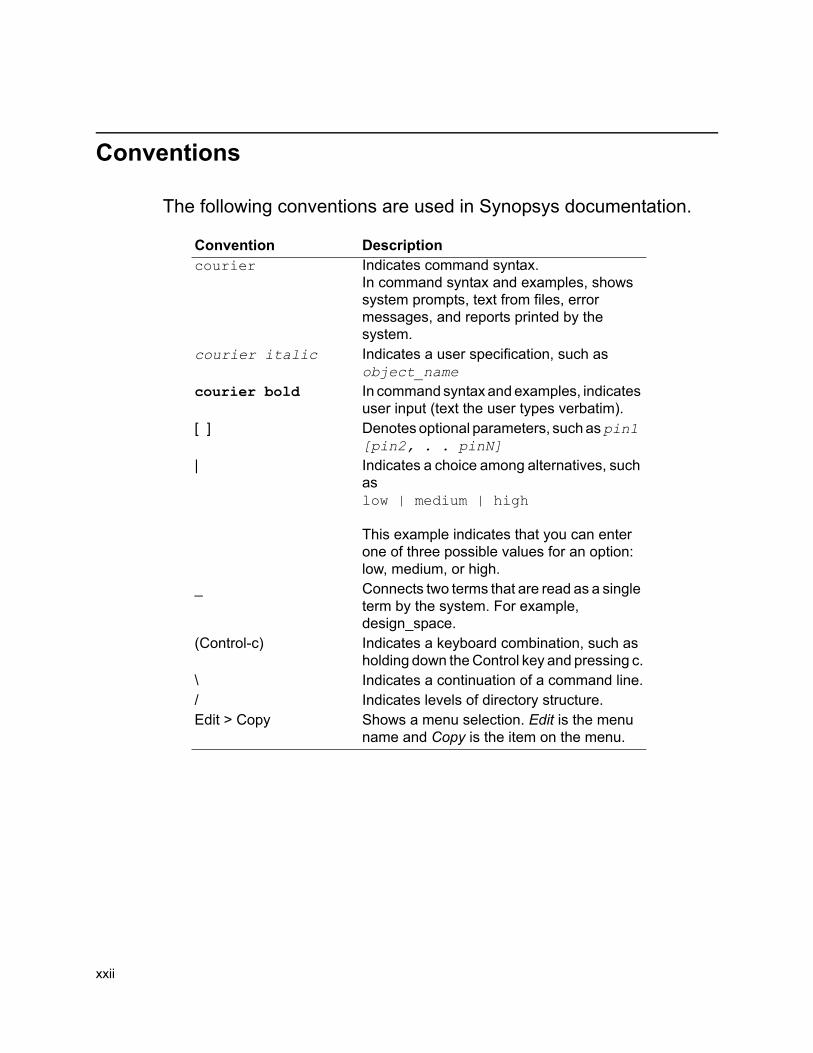
The following conventions are used in Synopsys documentation.
Convention Descriptioncourier Indicates command syntax.
In command syntax and examples, shows system prompts, text from files, error messages, and reports printed by the system.
courier italic Indicates a user specification, such as object_name
courier bold In command syntax and examples, indicates user input (text the user types verbatim).
[ ] Denotes optional parameters, such as pin1 [pin2, . . pinN]
| Indicates a choice among alternatives, such as low | medium | high
This example indicates that you can enter one of three possible values for an option: low, medium, or high.
_ Connects two terms that are read as a single term by the system. For example, design_space.
(Control-c) Indicates a keyboard combination, such as holding down the Control key and pressing c.
\ Indicates a continuation of a command line./ Indicates levels of directory structure.Edit > Copy Shows a menu selection. Edit is the menu
name and Copy is the item on the menu.
1-1
Getting Started
1Overview 1
VCS MX enables you to analyze, compile, and simulate Verilog, VHDL, and mixed-HDL design descriptions, and provides a set of simulation and debugging features to validate your design. These features provide capabilities for source-level debugging and simulation result viewing. VCS MX supports all levels of design descriptions, but is optimized for the behavioral and register transfer levels.
VCS MX accelerates complete system verification by delivering the fastest and highest capacity Verilog, VHDL, and Mixed-HDL simulation for RTL functional verification. The unique technology of VCS MX leverages cycle-based techniques with the flexibility of event-driven simulation to deliver its best performance for designs optimized for synthesis. The seamless support for mixed language simulation of VCS MX provides a high performance solution to your IP integration problems and gate level simulation.
1-2
Getting Started
In addition, VCS MX supports various Synopsys models and tools, like Synopsys DesignWare Models (SmartModels and LM-family hardware Modeler), DesignWare Foundation Library, VMC and VhMC Models, Telecom Workbench Models, MemPro Models, and VERA Testbench tool.
VCS MX is also integrated with other third-party tools via VHPI (for VHDL), PLI (for Verilog), and C language interface for VCS MX. The integration efforts include: testbench tools, memory models generation tools, acceleration and emulation systems, graphical user interfaces, and code coverage.
This chapter covers the following topics:
• What VCS MX Supports
• Setting up VCS MX
• Using VCS MX
What VCS MX Supports
VCS MX provides fully featured implementations of the following:
• The Verilog language as defined in the IEEE Standard Hardware Description Language Based on the Verilog Hardware Description Language (IEEE Std 1364-1995) and the Standard Verilog Hardware Description Language (IEEE Std 1364-2001).
• The VHDL Language as defined in the Standard VHDL Hardware Description Language (IEEE VHDL 1076-1993).
• The SystemVerilog 3.1a language (with some exceptions) as defined in SystemVerilog 3.1a Accellera’s Extensions to Verilog.
1-3
Getting Started
Setting up VCS MX
You must perfom the following tasks to set up your VCS MX environment. These tasks need to be performed only once.
• Setting Up Your Environment
• Creating the Setup File
Setting Up Your Environment
This section explains how to set up your VCS MX environment, including setting your VCS_HOME environment variable, your path to the simulation executables, and your VCS MX license environment.
To set up your environment, do the following:
1. Set your VCS_HOME environment variable by entering the following at the command line:
% setenv VCS_HOME VCS_MX_installation_directory
2. Set the path to your simulation executables by entering the following:
% setenv PATH .:${VCS_HOME}/bin:${PATH}
3. Set your VCS MX license environment by entering the following:
% setenv SNPSLMD_LICENSE_FILE Location_of_License_File
Note: A single VCS MX license (under Synopsys’ Common Licensing Program) enables you to run Verilog-only, VHDL-only, or mixed-HDL simulations.
1-4
Getting Started
For additional information on environment variables, see “VCS MX Environment Variables” in Chapter 2 in the VCS MX Reference Guide.
Creating the Setup File
VCS MX uses several setup files named SYNOPSYS_SIM.SETUP to set up and configure its environment for VHDL and mixed-HDL designs. These files map VHDL design library names to specific host directories, set search paths, and assign values to simulation control variables.
When you invoke VCS MX, it looks for the SYNOPSYS_SIM.SETUP files in the following three directories:
• Master setup directory
The SYNOPSYS_SIM.SETUP file in the /bin directory of the VCS MX installation directory contains default settings for your entire installation. VCS MX reads this file first.
• Your home directory
VCS MX reads the setup file in your home directory second, if present. The settings in this file override those in the master setup directory.
• Your design directory
VCS MX reads the setup file in your design directory last. The settings in this file override all others. You can use this file to customize the environment for a particular design. This is the directory you invoke and run VCS MX from; it is not the directory where you store or generate your design files.
1-5
Getting Started
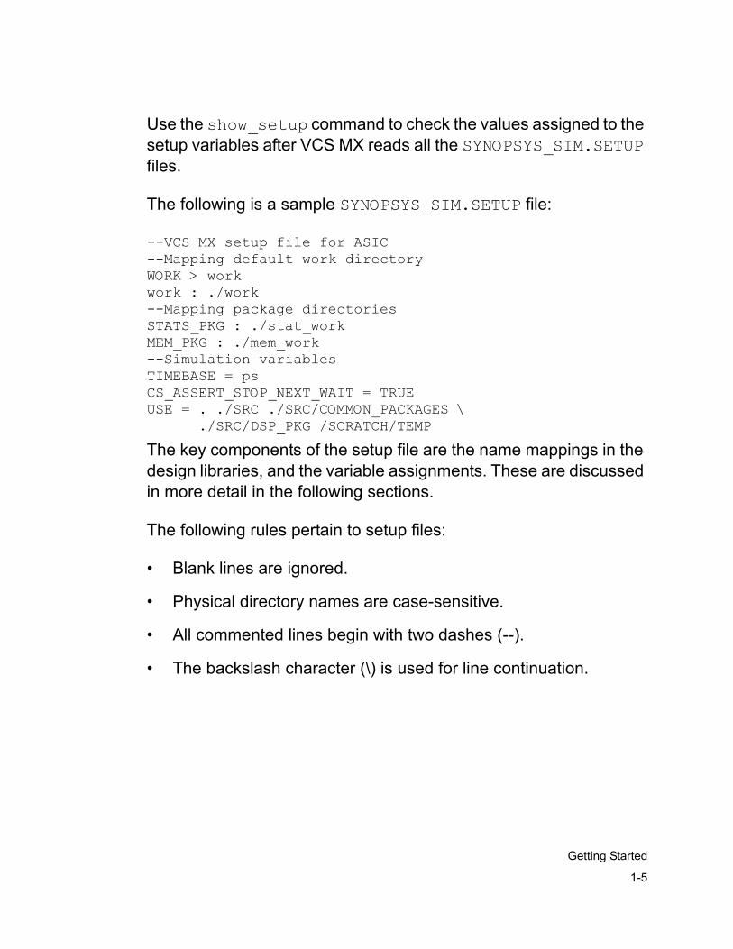
Use the show_setup command to check the values assigned to the setup variables after VCS MX reads all the SYNOPSYS_SIM.SETUP files.
The following is a sample SYNOPSYS_SIM.SETUP file:
--VCS MX setup file for ASIC--Mapping default work directoryWORK > workwork : ./work--Mapping package directoriesSTATS_PKG : ./stat_workMEM_PKG : ./mem_work--Simulation variablesTIMEBASE = psCS_ASSERT_STOP_NEXT_WAIT = TRUEUSE = . ./SRC ./SRC/COMMON_PACKAGES \ ./SRC/DSP_PKG /SCRATCH/TEMP
The key components of the setup file are the name mappings in the design libraries, and the variable assignments. These are discussed in more detail in the following sections.
The following rules pertain to setup files:
• Blank lines are ignored.
• Physical directory names are case-sensitive.
• All commented lines begin with two dashes (--).
• The backslash character (\) is used for line continuation.
1-6
Getting Started
Global Setup File
You can also specify a global setup file to define VCS MX setup variables. To do this, specify the file you want to use as the global setup file in the environment variable SYNOPSYS_SIM_SETUP. This global setup file may have any name, and doesn't have to be SYNOPSYS_SIM.SETUP or SYNOPSYS_VSS.SETUP. This file takes precedence over any regular setup file in the current directory, home directory, or installation directory, and is also searched during simulation, with the same restrictions as a setup file in the current directory. If the file name you specify in the SYNOPSYS_SIM_SETUP variable cannot be opened, VCS MX issues an error message.
Also, within a setup file, a line of the following form may exist:
OTHERS = <filename>
This includes and processes the named file. No environment substitution is done on this file. If the file cannot be opened, VCS MX issues an error message and stops, as the simulation may not run correctly.
Files included in this manner can be nested, with a limit of 8 levels of nesting.
Library Name Mapping
To use a VHDL design library with VCS MX, you must first map the VHDL identifier that designates the design library name (logical name) to the location of the library in the UNIX file system (physical name). You specify this mapping in the SYNOPSYS_SIM.SETUP file.
1-7
Getting Started
For greater flexibility in library naming, VCS MX provides two-stage mapping. You can first map the design library (logical name) to an intermediate name. You can then map the intermediate name to the physical name (a UNIX path name). This feature allows you to select different design units by simply changing the logical-to-intermediate mapping. The syntax is as follows:
logical_name > intermediate_nameintermediate_name : physical_name
For example, consider a case where you want to select between an 8-bit or a 16-bit ALU. You can pre-analyze the VHDL file for each component into a different physical directory. Then, by changing the mapping in the SYNOPSYS_SIM.SETUP file, you can choose which component you want to include in your design. As the following example illustrates, the design library (logical name) mapping uses the 8-bit adder instead of the 16-bit adder. The logical-to-intermediate name mapping is optional. If you specify only an intermediate-to-physical mapping, VCS MX assumes that the design library (logical) and intermediate names are identical.
ALU > ALU8ALU8 : ./alu_8bitALU16 : ./alu_16bit
The VCS MX built-in standard libraries have the following default name mappings:
IEEE : $VCS_HOME/$ARCH/packages/IEEE/libSYNOPSYS : $VCS_HOME/$ARCH/packages/synopsys/lib
In these default mappings, $ARCH is either sparcOS5, hpux10, or linux.
1-8
Getting Started
Use these built-in libraries in your design, whenever possible, to get maximum performance from the simulator.
Using VCS MX
This section provides an overview of the basic tasks you will need to do to run VCS MX. The following tasks are covered:
• Analyzing Your Design
• Compiling Your Design
• Simulating Your Design
Note: For information on coverage features, see the VCS /VCS MX Coverage Metrics User Guide.
Analyzing Your Design
If your design contains VHDL source code, it will need to be analyzed using the vhdlan utility. This process analyzes VHDL source files, produces intermediate files for elaboration, and saves these files into a library directory.
If your VHDL design instantiates a Verilog design within it, you will need to use the vlogan command.
For details on how to analyze your design, see “Analyzing Your Design” in Chapter 4.
1-9
Getting Started
Compiling Your Design
The compilation phase compiles your source code into a single simulation executable. Depending on the components of your design, there are two different methods you can use for compilation:
• If you are running a simulation containing only VHDL code (referred to throughout this manual as a "VHDL-only" simulation) or a mixed-HDL simulation by instantiating Verilog code with VHDL (referred to throughout this manual as "VHDL-top"), you will use the scs command to compile your design. The scs command elaborates your design, performs code generation, C compilation, and static linking of all objects to generate an executable binary file (called scsim) for running the simulation. For a detailed description of how to instantiate Verilog into VHDL, see the “Instantiating Verilog in a VHDL Design within Verilog” on page 3-21.
• If you are running a simulation containing only Verilog code (referred to throughout this manual as "Verilog-only") or a mixed-HDL simulation by instantiating VHDL code within Verilog (referred to throughout this manual as "Verilog-top"), you will use the vcs command to compile your design and create a simulation executable named simv. The vcs command compiles your code on a module by module basis, which enables incremental compilation. For a detailed description of how to instantiate VHDL into Verilog, see “Instantiating a VHDL Design within a Verilog Design” on page 3-12.
For details on the various options you can run at the command line during compilation, see “Compilation Options” in Chapter 4 of the VCS MX Reference Guide.
1-10
Getting Started
Simulating Your Design
In the simulation phase, at the command line you enter the simulation executable produced by the complilation phase:
• For VHDL-only or VHDL-top: scsim
• For Verilog-only or Verilog-top: simv.
You can also add various simulation run-time options. For details, see “Simulation Executables and Options” in Chapter 5 of the VCS MX Reference Guide.
For details on simulating your design, see “Simulating Your Design” in Chapter 7.
Discovery Visual Environment (DVE) software is a graphical verification environment that supports debugging for VCS MX simulations. DVE allows you to work in post-processing and interactive mode. We would encourage you to use DVE as a default GUI for debugging, to view simulations and more. For more details on DVE, see “Discovery Visual Environment” in Chapter 9
2-1
VCS MX Reference Flows
2VCS MX Reference Flows 1
Depending on the contents of your design, VCS MX offers a variety of simulation flows. This section covers the following topics:
• Mixed-HDL Simulation Basics
• VHDL-Only Flow Overview
• Verilog-Only Flow Overview
• VHDL-Top Flow Overview
• Verilog-Top Flow Overview
2-2
VCS MX Reference Flows
Mixed-HDL Simulation Basics
The VCS MX engine can simulate mixed language designs from within the VCS MX environment, while retaining all existing VHDL and Verilog tool links and flows.
This section provides a brief overview of the basic flows you can use in VCS MX, along with information on RTL/Bbehaviorial simulation, gate-level simulation, and general restrictions.
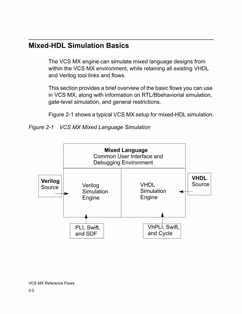
Figure 2-1 shows a typical VCS MX setup for mixed-HDL simulation.
Figure 2-1 VCS MX Mixed Language Simulation
Mixed LanguageCommon User Interface andDebugging Environment
VerilogSimulationEngine
VHDLSimulationEngine
PLI, Swift,and SDF
VhPLI, Swift,and Cycle
VerilogSource
VHDLSource
2-3
VCS MX Reference Flows
In general, you can use the following flows for performing to perform simulations in VCS MX:
• "VHDL-Only" Flow
In this flow, you use a VHDL testbench and VHDL source code. You will analyze your design using the vhdlan utility, compile your design using the scs executable, and simulate your design using the scsim executable. This flow is referred to throughout this manual as the "VHDL-only" flow. For more information on this flow, see “VHDL-Only Flow Overview” on page 2-6.
• "Verilog-Only" Flow
In this flow, you use a Verilog testbench and Verilog source code. You will compile your design using the vcs executable, and simulate your design using the simv executable. This flow is referred to throughout this manual as the "Verilog-Oonly" flow. For more information, see “Verilog-Only Flow Overview” on page 2-9.
• "VHDL-Top" Flow
In this flow, you use a VHDL testbench, with your VHDL and Verilog code instantiated in lower levels of hierarchy. You analyze your VHDL code using the vhdlan utility and your Verilog code using the vlogan utility, compile your code using the scs executable and -mhdl command line option, and simulate your design using the scsim executable. This flow is referred to throughout this manual as the "VHDL-Ttop" flow. For more information on this flow, see “VHDL-Top Flow Overview” on page 2-11.
2-4
VCS MX Reference Flows
• "Verilog-Top" Flow
In this flow, you use a Verilog testbench, with your Verilog and VHDL code instantiated in lower levels of hierarchy. You analyze the VHDL portion of your code using the using the vhdlan utility and the Verilog portion of your design (if itsit is instantiated within VHDL) using the vlogan utility, compile your code using the vcs executable and -mhdl command line option, and simulate your design using the simv executable. This flow is referred to throughout this manual as the "Verilog-Ttop" flow. For more information on this flow, see “Verilog-Top Flow Overview” on page 2-14.
Note:Note that i In VCS MX, the simulation environments needed for mixed language simulation are the same as those used for Verilog and VHDL are needed for mixed language simulation. This eliminates the need for learning a new environment, and you do not need to generate, modify, compile/analyze, or maintain additional shells. Instantiation of Verilog design units in VHDL, and vice versa is seamless.
RTL/Behavioral Level Simulation
In all VCS MX flows, the VHDL and Verilog portions parts of your designs can be behavioral, RTL, or a mix of both. Both VHDL and Verilog code can run in event mode, cycle mode, or mixed event and cycle mode. You can specify various optimizations and code-generation switches for both VHDL and Verilog portions parts of the design.
2-5
VCS MX Reference Flows
Performance is improved improves when you use VCS MX RTL event and cycle simulation for the VHDL part of the design portion and RTL simulation capabilities for the Verilog part of the design portions. The VHDL portion part can be run in event mode or mixed event and cycle mode, depending on how much of itportion is cycle compliant. For more information on s cycle simulation, see “Compiling and Elaborating Your Design” in Chapter 5.
Gate-Level Simulation
For VHDL gate-level simulation, VCS MX supports VHDL netlist simulation using VHDL initiative toward ASIC libraries (VITAL). However, there is always a performance penalty when using using VITAL, either (with or without Standard Delay Format (SDF) DF back-annotation). So, in order to obtain the highest performance, it is recommended you you should use a VHDL testbench and Verilog netlist when peforming mixed language simulation. Full timing simulation with SDF back-annotation is supported for Verilog netlist.
The following section describes the basics of VCS MX simulator for users who might not be are not familiar with the either simulator engine.
Restrictions
In the Verilog-only and Verilog-top flows, the following restrictions apply:
• VCS MX does not cannot handle 64-bit compilation and 64-32 bit cross-compilation.
2-6
VCS MX Reference Flows
• The Debussy interface only works interactively only on the Verilog part of the design,. but However, Debussy supports post processing with fsdb files in both the Verilog and VHDL parts of the design using the latest Debussy release.
• There are limitations on the data types of the ports and generics in the top-level VHDL design entity that you instantiate into the Verilog design,. For details, see See “Instantiating a VHDL Design within a Verilog Design” in Chapter 3.
• You can’t use the VirSim Logic Browser or Event Origin feature in the VHDL part of the design.
• You can generate profile reports for both the Verilog and VHDL parts of the design during the same simulation, generating two separate reports. However, VCS MX writes the : one report for the Verilog part written by VCS MX in text format, and the otherreport for the VHDL part, written by VCS MX in HTML format.
• PLI applications only work only with the Verilog part of a mixed HDL design.
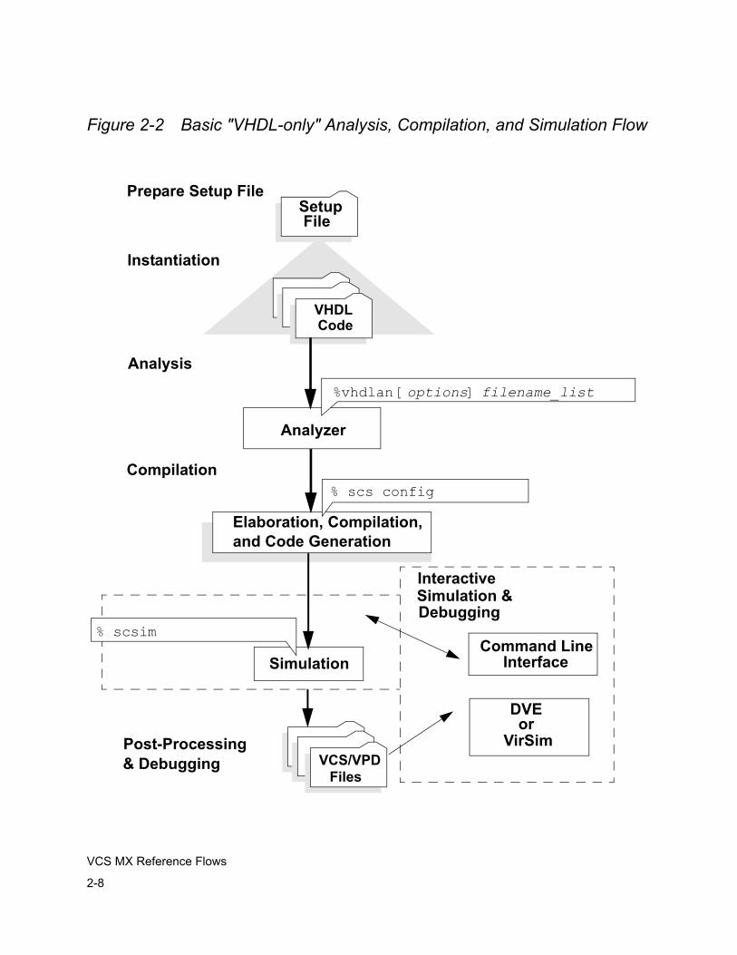
VHDL-Only Flow Overview
This section explains the VCS MX verification flow that applies if your design contains only VHDL code.
The basic steps for performing a VHDL-only simulation are as follows:
1. Set up your environment. For details, see “Setting Up Your Environment” on page 1-3.
2. Create the setup file for VHDL simulation. For details, see “Creating the Setup File” on page 1-4
2-7
VCS MX Reference Flows
3. Analyze your design. For details, see “Analyzing Your Design” in Chapter 4.
4. Compile and Eelaborate the entire design. For details, see “Compiling and Elaborating Your Design” in Chapter 5.
5. Simulate the design. For details, see “Simulating Your Design” in Chapter 7.
6. Use DVE or VirSim to control and view simulation events interactively during simulation, or post-process the results using the simulation history file. Post-process the results using DVE or VirSim. You can also use DVE or VirSim interactively
See Figure 2-2 below for a VHDL-only flow chart.
2-8
VCS MX Reference Flows
Figure 2-2 Basic "VHDL-only" Analysis, Compilation, and Simulation Flow
Simulation
Compilation% scs config
VCS/VPDFiles
% scsimCommand Line
Interface
Debugging
VHDLCode
Prepare Setup File
Simulation &
SetupFile
Interactive
Post-Processing& Debugging
Analysis
Analyzer
%vhdlan [options] filename_list
Instantiation
Elaboration, Compilation, and Code Generation
or VirSim
DVE
2-9
VCS MX Reference Flows
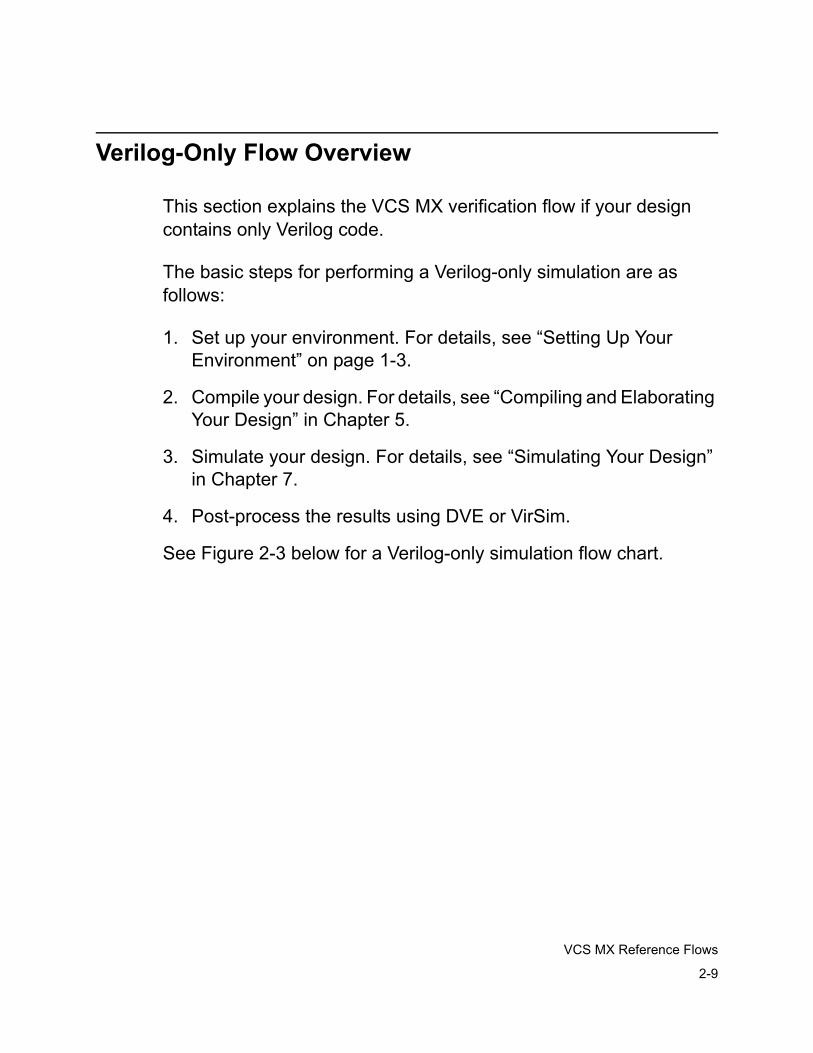
Verilog-Only Flow Overview
This section explains the VCS MX verification flow if your design contains only Verilog code.
The basic steps for performing a Verilog-only simulation are as follows:
1. Set up your environment. For details, see “Setting Up Your Environment” on page 1-3.
2. Compile your design. For details, see “Compiling and Elaborating Your Design” in Chapter 5.
3. Simulate your design. For details, see “Simulating Your Design” in Chapter 7.
4. Post-process the results using DVE or VirSim.
See Figure 2-3 below for a Verilog-only simulation flow chart.
2-10
VCS MX Reference Flows
Figure 2-3 Basic Verilog-only Compilation and Simulation Flow
Compilation
% vcs mem.v cpu.v
VerilogCode
(mem.v, cpu.v)
VCD/VPDFiles
Simulation
% simvCommand Line
Interface
Interactive Debugging
Post-Processing/Debugging
or VirSim
DVE
2-11
VCS MX Reference Flows
VHDL-Top Flow Overview
This section explains the VCS MX verification flow that applies if your design contains mixed-HDL code with Verilog code instantiated within VHDL code. You can, in turn, instantiate a VHDL design in the instantiated Verilog design.
This flow generates a VCD+ simulation history file that enables you to use DVE or VirSim after simulation to view the simulation results from of both the VHDL and Verilog parts of the design. You can also use DVE or VirSim to interactively simulate and debug this flow.
The basic steps in the VHDL-top flow are as follows:
1. Set up your environment. For details, see “Setting Up Your Environment” on page 1-3.
2. Create the setup file for VHDL simulation. For details, see “Creating the Setup File” on page 1-4.
3. Instantiate the Verilog modules in the VHDL design using component declarations and component instantiations. For details, see “Instantiating a Verilog Design in a VHDL Design” on page 3-2.
4. Analyze Verilog and VHDL modules and design units. This includes including their dependencies. See “Analyzing Your Design” in Chapter 4 for information on running vhdlan to analyze your VHDL code.
5. Compile and Eelaborate the entire design using the scs command and -mhdl flag. For details, see “Compiling and Elaborating Your Design” in Chapter 5.
2-12
VCS MX Reference Flows
6. Simulate the design using the simv executable. For details, see “Simulating Your Design” in Chapter 7.
7. Use DVE or VirSim to control and view simulation events interactively during simulation, or post-process the results using the simulation history file. Post-process the results using DVE or VirSim. You can also use DVE or VirSim interactively.
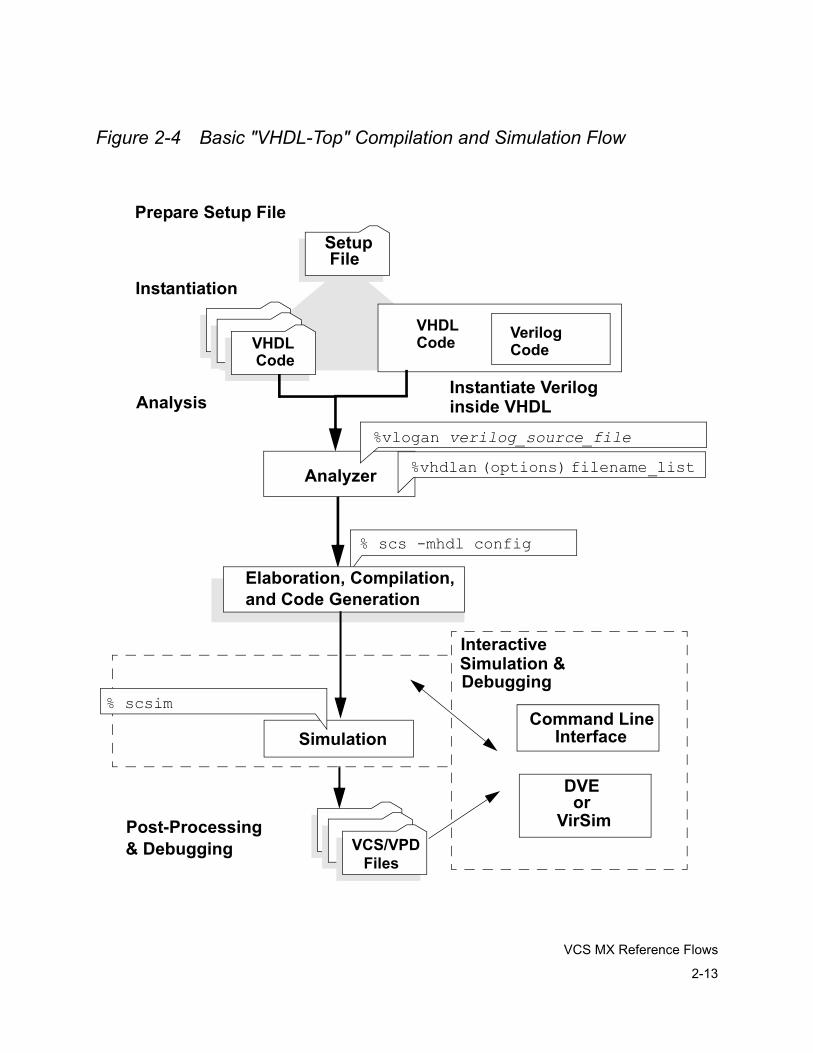
See Figure 2-4 below for a graphic that explains the VHDL-top simulation flow chartflow.
2-13
VCS MX Reference Flows
Figure 2-4 Basic "VHDL-Top" Compilation and Simulation Flow
VCS/VPDFiles
Simulation
% scsim Command Line
Interface
Debugging
VHDLCode
VHDLCode Verilog
Code
Prepare Setup File
Simulation &
SetupFile
Interactive
Post-Processing& Debugging
AnalysisInstantiate Veriloginside VHDL
Analyzer
Instantiation
% scs -mhdl config
%vlogan verilog_source_file
Elaboration, Compilation, and Code Generation
%vhdlan (options) filename_list
or VirSim
DVE
2-14
VCS MX Reference Flows
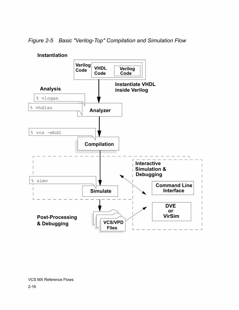
Verilog-Top Flow Overview
This section explains the VCS MX verification flow that applies if your design contains mixed-HDL code with VHDL code instantiated within Verilog code. You can, in turn, instantiate a Verilog design in the instantiated VHDL design.
This flow generates a VCD+ simulation history file that enables you to use DVE or VirSim after simulation to view the simulation results of from both the VHDL and Verilog parts of the design. You can also use DVE or VirSim to interactively simulate and debug this flow.
The steps in the Verilog-top flow are as follows:
1. Set up your environment. For details, see “Setting Up Your Environment” on page 1-3.
2. Create the setup file for VHDL simulation, see “Creating the Setup File” on page 1-4.
3. Analyze the VHDL code in the VHDL design that you need to instantiate in a Verilog design using the vhdlan utility, and analyze Verilog code instantiated within VHDL using the vlogan utility. This includes the dependencies. See “Analyzing Your Design” in Chapter 4 for information on running vhdlan to analyze your VHDL code.
4. Instantiate the VHDL design entity into a Verilog module definition.This is done with using a module instantiation statement.
5. If you need it, iInstantiate a Verilog module into a VHDL architecture if you need to do so. This is done with You can do this using a component declaration and component instantiation statement.
2-15
VCS MX Reference Flows
6. Compile the Verilog part of the design, and compile and elaborate the VHDL part of the design, using the vcs command line and-mhdl option. For details, see “Compiling and Elaborating Your Design” in Chapter 5.
7. Run the simulation using a simv command line (see “Simulating Your Design” in Chapter 7). Steps 6 and 7 can be combined into a single step with the -R or -RI option.
8. Use DVE or VirSim to control and view simulation events interactively during simulation, or post-process the results using the simulation history file. Post-process the results using DVE or VirSim. You can also use DVE or VirSim interactively.
See Figure 2-5 below for a graphic that explains the flow. for a graphic that explains the Verilog-Top simulation flow chartflow.
2-16
VCS MX Reference Flows
Figure 2-5 Basic "Verilog-Top" Compilation and Simulation Flow
Simulate
Compilation
% vcs -mhdl
VCS/VPDFiles
% simv Command Line
Interface
Debugging
VerilogCode VHDL
Code
Simulation &Interactive
Post-Processing& Debugging
AnalysisInstantiate VHDLinside Verilog
Analyzer% vhdlan
CodeVerilog
Instantiation
% vlogan
or VirSim
DVE
3-1
Instantiating Verilog or VHDL in Your Design
3Instantiating Verilog or VHDL in Your Design 2
This chapter describes the following instantiation processes:
• Instantiating a Verilog Design in a VHDL Design
• Instantiating a VHDL Design within a Verilog Design
Note that both of these processes are closely connected to the analysis process described “Analyzing Your Design” in Chapter 3. The analysis and instantiation processes overlap in many situations discussed in the chapter.
3-2
Instantiating Verilog or VHDL in Your Design
Instantiating a Verilog Design in a VHDL Design
You can instantiate a module of a Verilog design into a VHDL design the same way you instantiate a VHDL component — by using a component declaration and a component instantiation statement.
Although the port order in the component declaration can be the same or different than the port declaration order in the corresponding Verilog module definition, it is highly recommended that you keep it the same.
Parameters in Verilog modules can be declared as VHDL generics in corresponding VHDL component declaration (this is suggested but it is not a required). You can pass actual values to those generics during actual component instantiation. In case of no mapping, default values will be used for simulation.
You can use the following data types to specify ports in the component declaration:
• bit
• std_logic
• std_ulogic
• bit_vector
• std_logic_vector
• std_ulogic_vector
• std_logic_arith
• boolean
3-3
Instantiating Verilog or VHDL in Your Design
• buffer
buffer type is actually supported only when a Verilog module instanciates a VHDL component.
• User-defined types and subtypes, as long as the basic type of the element type is in std_nlogic bit and boolean.
• Unconstrained vector VHDL port.
• Function call at VHDL port size expression.
• VHDL signed/unsigned to Verilog wire signed.
You can use vector data types for vector ports in the Verilog module. VCS MX includes built-in data type conversion for these VHDL data types to Verilog data types.
In addition, you can instantiate a Verilog module having port of type signed can be instantiated in a VHDL design unit (architecture). See “Signed and Unsigned Type Support” on page 2-4.
If the module definition contains parameter declarations, the corresponding component declaration specifies generics that match the parameter names as shown in the next example.
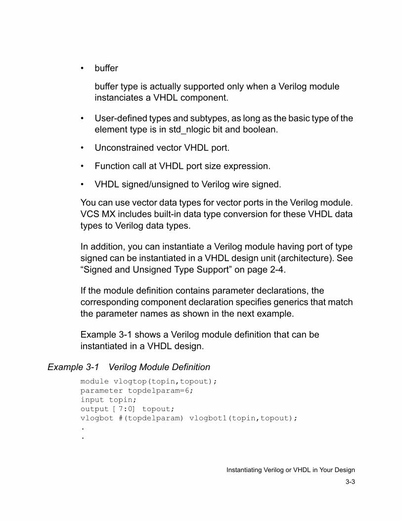
Example 3-1 shows a Verilog module definition that can be instantiated in a VHDL design.
Example 3-1 Verilog Module Definitionmodule vlogtop(topin,topout);parameter topdelparam=6;input topin;output [7:0] topout;vlogbot #(topdelparam) vlogbot1(topin,topout);..
3-4
Instantiating Verilog or VHDL in Your Design
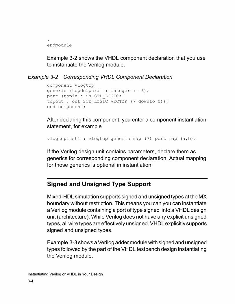
.endmodule
Example 3-2 shows the VHDL component declaration that you use to instantiate the Verilog module.
Example 3-2 Corresponding VHDL Component Declarationcomponent vlogtopgeneric (topdelparam : integer := 6);port (topin : in STD_LOGIC;topout : out STD_LOGIC_VECTOR (7 downto 0));end component;
After declaring this component, you enter a component instantiation statement, for example
vlogtopinst1 : vlogtop generic map (7) port map (a,b);
If the Verilog design unit contains parameters, declare them as generics for corresponding component declaration. Actual mapping for those generics is optional in instantiation.
Signed and Unsigned Type Support
Mixed-HDL simulation supports signed and unsigned types at the MX boundary without restriction. This means you can you can instantiate a Verilog module containing a port of type signed into a VHDL design unit (architecture). While Verilog does not have any explicit unsigned types, all wire types are effectively unsigned. VHDL explicitly supports signed and unsigned types.
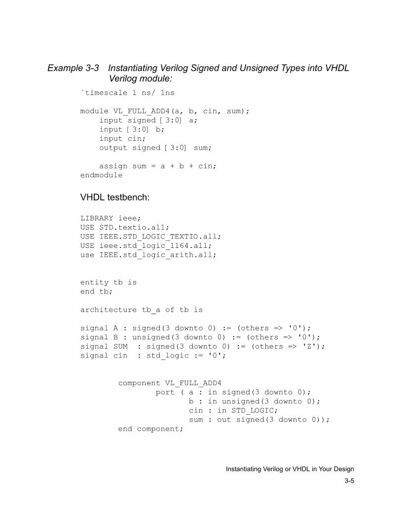
Example 3-3 shows a Verilog adder module with signed and unsigned types followed by the part of the VHDL testbench design instantiating the Verilog module.
3-5
Instantiating Verilog or VHDL in Your Design
Example 3-3 Instantiating Verilog Signed and Unsigned Types into VHDL Verilog module:
`timescale 1 ns/ 1ns
module VL_FULL_ADD4(a, b, cin, sum); input signed [3:0] a; input [3:0] b; input cin; output signed [3:0] sum;
assign sum = a + b + cin;endmodule
VHDL testbench:
LIBRARY ieee;USE STD.textio.all;USE IEEE.STD_LOGIC_TEXTIO.all;USE ieee.std_logic_1164.all;use IEEE.std_logic_arith.all;
entity tb isend tb; architecture tb_a of tb is signal A : signed(3 downto 0) := (others => '0');signal B : unsigned(3 downto 0) := (others => '0');signal SUM : signed(3 downto 0) := (others => 'Z');signal cin : std_logic := '0';
component VL_FULL_ADD4 port ( a : in signed(3 downto 0); b : in unsigned(3 downto 0); cin : in STD_LOGIC; sum : out signed(3 downto 0)); end component;
3-6
Instantiating Verilog or VHDL in Your Design
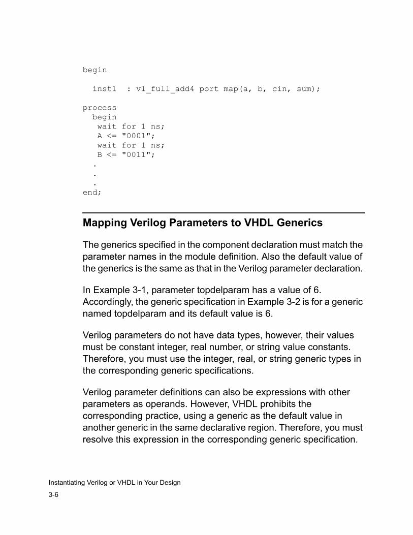
begin inst1 : vl_full_add4 port map(a, b, cin, sum); process begin wait for 1 ns; A <= "0001"; wait for 1 ns; B <= "0011"; . . .end;
Mapping Verilog Parameters to VHDL Generics
The generics specified in the component declaration must match the parameter names in the module definition. Also the default value of the generics is the same as that in the Verilog parameter declaration.
In Example 3-1, parameter topdelparam has a value of 6. Accordingly, the generic specification in Example 3-2 is for a generic named topdelparam and its default value is 6.
Verilog parameters do not have data types, however, their values must be constant integer, real number, or string value constants. Therefore, you must use the integer, real, or string generic types in the corresponding generic specifications.
Verilog parameter definitions can also be expressions with other parameters as operands. However, VHDL prohibits the corresponding practice, using a generic as the default value in another generic in the same declarative region. Therefore, you must resolve this expression in the corresponding generic specification.
3-7
Instantiating Verilog or VHDL in Your Design
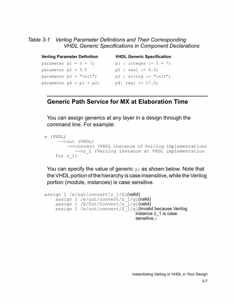
Table 3-1 Verilog Parameter Definitions and Their Corresponding VHDL Generic Specifications in Component Declarations
Generic Path Service for MX at Elaboration Time
You can assign generics at any layer in a design through the command line. For example:
e (VHDL) -->uut (VHDL) -->convert (VHDL instance of Verilog implementation) -->z_1 (Verilog instance at VHDL implementation for z_1)
You can specify the value of generic g1 as shown below. Note that the VHDL portion of the hierarchy is case insensitive, while the Verilog portion (module, instances) is case sensitive.
assign 1 /e/uut/convert/z_1/G1(valid)assign 1 /e/uut/convert/z_1/g1(valid)assign 1 /E/Uut/Convert/z_1/g1(valid)assign 1 /e/uut/convert/Z_1/g1(Invalid because Verilog instance z_1 is case
sensitive.)
Verilog Parameter Definition VHDL Generic Specificationparameter p1 = 5 + 7; p1 : integer := 5 + 7;
parameter p2 = 5.5 p2 : real := 5.5;
parameter p3 = "init"; p3 : string := "init";
parameter p4 = p1 + p2; p4: real := 17.5;
3-8
Instantiating Verilog or VHDL in Your Design
Mapping Verilog Ports to VHDL Ports
The port names in the VHDL component declaration must match the port names in the Verilog module definition.
The mode or direction of the in, out, or inout ports in the VHDL component declaration must match the type of input, output, or inout port declaration in the Verilog module definition.
The size or bit-width and the bit values used to specify the bit-width, of the ports in the VHDL component declaration must match the bit-width and bit values in the port declarations in the Verilog module definition.
In Example 3-1, port topin is a scalar input port and in Example 3-2, port topin is also a scalar port of mode in with a scalar data type. In Example 3-1, port topout is an eight bit vector output port with the bits numbered from 7 to 0 and in Example 3-2, port topout is also an eight bit vector port of mode out with the bits numbered from 7 downto 0.
In Example 3-2 port topin has the STD_LOGIC data type because this is a valid data type for converting values from VHDL to Verilog and port topin is a scalar port. Also in Example 3-2 port topout has the STD_LOGIC_VECTOR data type because this also is a valid data type for converting values from Verilog to VHDL and port topout is a vector port.
Instantiating a Verilog Module with Parameterized Ports
In Verilog, a port can be parameterized so that its bit-width is specified using a parameter. This allows you to use parameter passing into an instance of the module for the bit-width that enables a port to have different bit-widths in different instances of the same module.
3-9
Instantiating Verilog or VHDL in Your Design
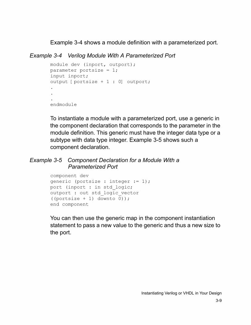
Example 3-4 shows a module definition with a parameterized port.
Example 3-4 Verilog Module With A Parameterized Portmodule dev (inport, outport);parameter portsize = 1;input inport;output [portsize + 1 : 0] outport;...endmodule
To instantiate a module with a parameterized port, use a generic in the component declaration that corresponds to the parameter in the module definition. This generic must have the integer data type or a subtype with data type integer. Example 3-5 shows such a component declaration.
Example 3-5 Component Declaration for a Module With a Parameterized Port
component devgeneric (portsize : integer := 1);port (inport : in std_logic;outport : out std_logic_vector((portsize + 1) downto 0));end component
You can then use the generic map in the component instantiation statement to pass a new value to the generic and thus a new size to the port.
3-10
Instantiating Verilog or VHDL in Your Design
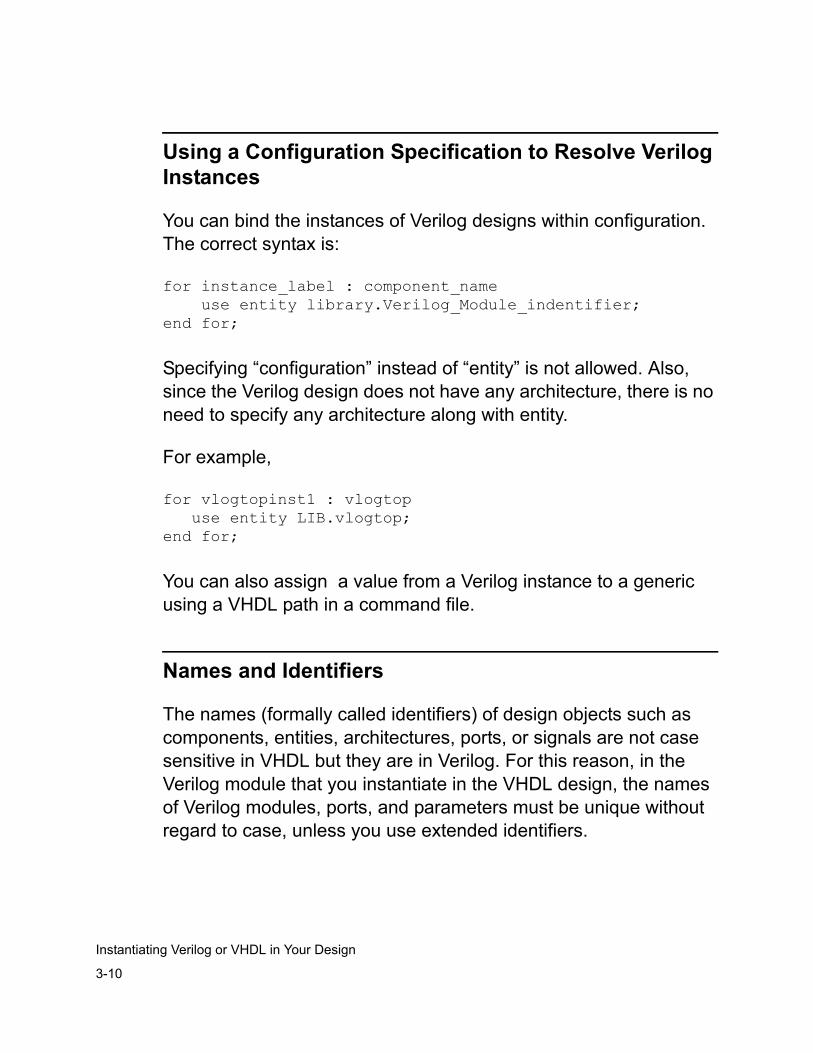
Using a Configuration Specification to Resolve Verilog Instances
You can bind the instances of Verilog designs within configuration. The correct syntax is:
for instance_label : component_name use entity library.Verilog_Module_indentifier;end for;
Specifying “configuration” instead of “entity” is not allowed. Also, since the Verilog design does not have any architecture, there is no need to specify any architecture along with entity.
For example,
for vlogtopinst1 : vlogtop use entity LIB.vlogtop;end for;
You can also assign a value from a Verilog instance to a generic using a VHDL path in a command file.
Names and Identifiers
The names (formally called identifiers) of design objects such as components, entities, architectures, ports, or signals are not case sensitive in VHDL but they are in Verilog. For this reason, in the Verilog module that you instantiate in the VHDL design, the names of Verilog modules, ports, and parameters must be unique without regard to case, unless you use extended identifiers.
3-11
Instantiating Verilog or VHDL in Your Design
For example, in Verilog you can specify the following two input port names: in1 and IN1, but not in VHDL. Therefore, you must change one of the port names if the port is in the top-level module of the Verilog design that you are instantiating in your VHDL design. You cannot use VHDL keywords as the names of modules, ports, or parameters in the top-level module, unless you use extended identifiers.
You must follow the rules for VHDL identifiers in the names of modules, ports, or parameters in the top-level module. Valid VHDL identifiers consist of upper or lower case letters, numbers, and the underscore, the first character must be a letter, and the last character cannot be the underscore character (_), unless you use extended identifiers.
Using Extended Identifiers
You can use extended identifiers (similar to Verilog escaped identifiers) to fulfill the rules for VHDL identifiers, for example,
• You can specify ports \in1\ and \IN1\ in the component declaration.
• You can specify an entity named \component\.
• You can begin a name with a number and end with an underscore, such as an architecture named \1comparch_\.
Module Header Port List Restrictions
The port list in the module header for the instantiated module cannot contain either of the following:
• Unconnected ports
3-12
Instantiating Verilog or VHDL in Your Design
• Jumpered ports
An unconnected port is an empty space between commas in the port connection list, for example,
module vlogtop (portia, , portib);
A jumpered port is a port that appears more than once in the port list, for example,
module vlogtop (portia, portia);
Instantiating a VHDL Design within a Verilog Design
You can instantiate the top-level design entity (entity and architecture) of a VHDL design within a Verilog design the same way that you instantiate a Verilog module: with a module instantiation statement.
In the module instantiation statement you can specify the following:
• The entity name of the top level design entity, see Example 3-1 and Example 3-2.
You don’t specify the architecture when you specify the entity. During elaboration, the scs compiler uses the most recently compiled architecture for the entity. VCS MX’s VHDL elaboration happens when you compile the Verilog part of the design.
• The configuration name of the configuration that specifies the entity and architecture of the top-level design entity, see Example 3-3 and Example 3-4.
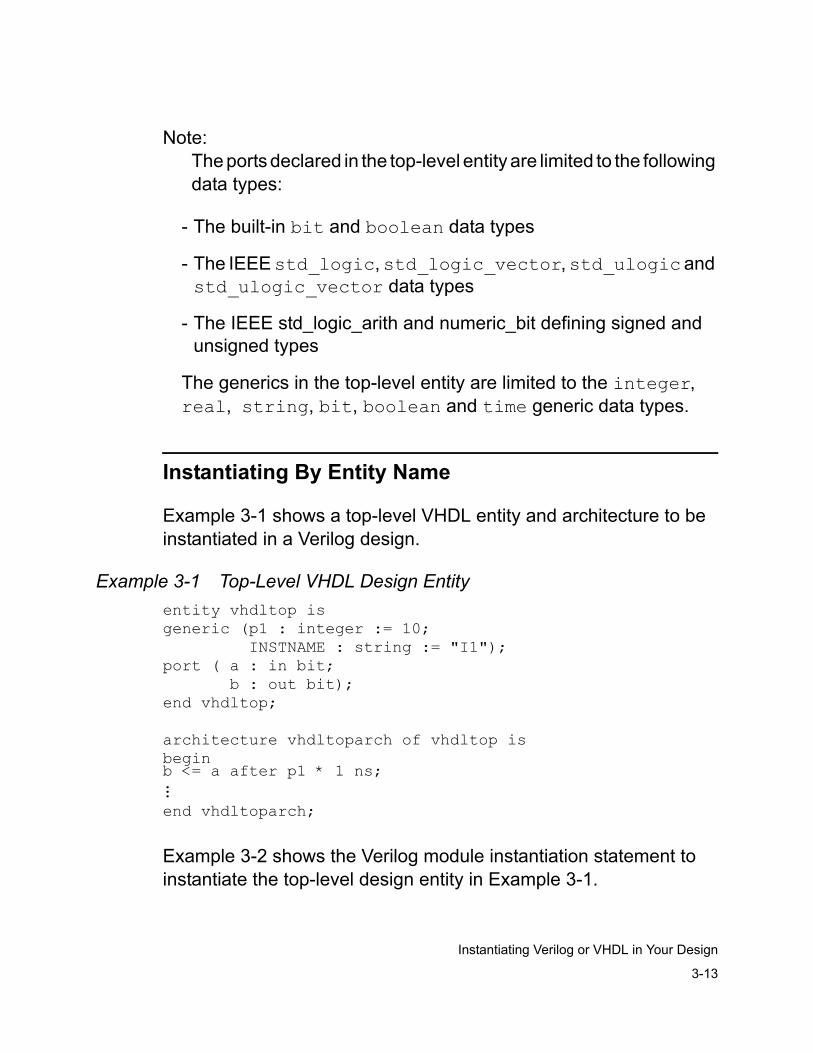
3-13
Instantiating Verilog or VHDL in Your Design
Note:The ports declared in the top-level entity are limited to the following data types:
- The built-in bit and boolean data types
- The IEEE std_logic, std_logic_vector, std_ulogic and std_ulogic_vector data types
- The IEEE std_logic_arith and numeric_bit defining signed and unsigned types
The generics in the top-level entity are limited to the integer, real, string, bit, boolean and time generic data types.
Instantiating By Entity Name
Example 3-1 shows a top-level VHDL entity and architecture to be instantiated in a Verilog design.
Example 3-1 Top-Level VHDL Design Entityentity vhdltop isgeneric (p1 : integer := 10; INSTNAME : string := "I1");port ( a : in bit; b : out bit);end vhdltop;
architecture vhdltoparch of vhdltop isbeginb <= a after p1 * 1 ns;...end vhdltoparch;
Example 3-2 shows the Verilog module instantiation statement to instantiate the top-level design entity in Example 3-1.

3-14
Instantiating Verilog or VHDL in Your Design
Example 3-2 The Verilog Module Instantiation Statement For The Entityvhdltop #(15,"myInst") vhdltopinst (rega,wireb);
In Example 3-2 the module identifier vhdltop matched the entity name of the top-level entity in Example 3-1 and the parameter passing assignment part passes new values, the integer 15 and the string “myInst”, to the generics in Example 3-1. Verilog reg rega and wire wireb attach to the VHDL ports a and b.
Instantiating By Configuration Name
Example 3-3 Configuration For The Top-Level VHDL Design Entityconfiguration vhdltop_cfg of vhdltop is for vhdltoparch . . . end for;end configuration;
This configuration is for the entity and architecture in Example 3-1. Example 3-4 shows the Verilog module instantiation statement to instantiate this configuration.
Example 3-4 The Verilog Module Instantiation Statement For The Configuration
vhdltop_cfg #(15,"myInst") vhdltopinst (rega,wireb);
Similar to Example 3-2, in Example 3-4 the module identifier vhdltop_cfg matched the name of the configuration in Example 3-3. VCS instantiates the design entity specified by this configuration.
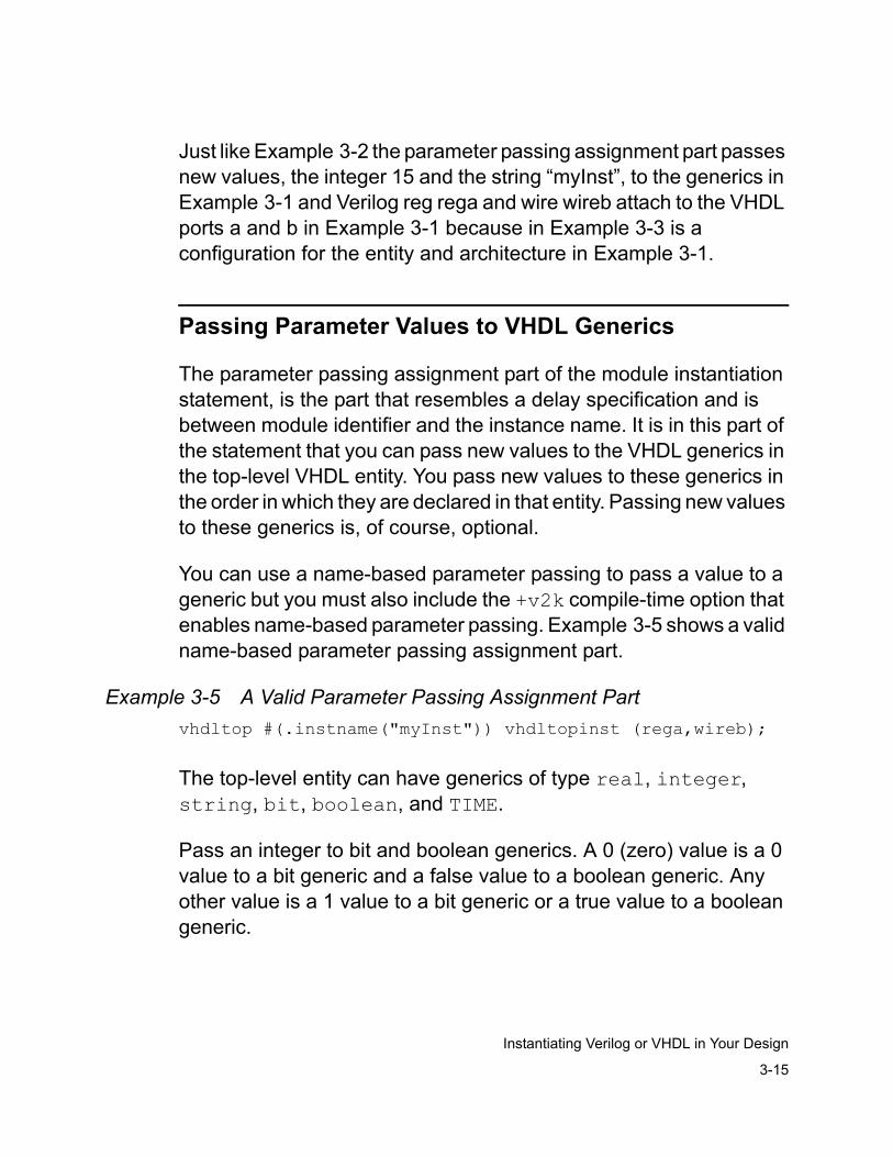
3-15
Instantiating Verilog or VHDL in Your Design
Just like Example 3-2 the parameter passing assignment part passes new values, the integer 15 and the string “myInst”, to the generics in Example 3-1 and Verilog reg rega and wire wireb attach to the VHDL ports a and b in Example 3-1 because in Example 3-3 is a configuration for the entity and architecture in Example 3-1.
Passing Parameter Values to VHDL Generics
The parameter passing assignment part of the module instantiation statement, is the part that resembles a delay specification and is between module identifier and the instance name. It is in this part of the statement that you can pass new values to the VHDL generics in the top-level VHDL entity. You pass new values to these generics in the order in which they are declared in that entity. Passing new values to these generics is, of course, optional.
You can use a name-based parameter passing to pass a value to a generic but you must also include the +v2k compile-time option that enables name-based parameter passing. Example 3-5 shows a valid name-based parameter passing assignment part.
Example 3-5 A Valid Parameter Passing Assignment Partvhdltop #(.instname("myInst")) vhdltopinst (rega,wireb);
The top-level entity can have generics of type real, integer, string, bit, boolean, and TIME.
Pass an integer to bit and boolean generics. A 0 (zero) value is a 0 value to a bit generic and a false value to a boolean generic. Any other value is a 1 value to a bit generic or a true value to a boolean generic.
3-16
Instantiating Verilog or VHDL in Your Design
Pass a Verilog string to a TIME generic. The TIME type has both a value and a unit so include both in the string, for example:
vhdltop #(.myTIME("10 ns")) vhdltopinst (rega,wireb);
You can use integer and real generic types to pass delay values to the VHDL design. The VHDL design multiplies the integer or real value with a time value. In Example 3-1 generic p1, of the integer type with the default value of 10, is used as delay value for a concurrent signal assignment statement. In the parameter passing assignment part of the module instantiation statement in Example 3-2, a new value of 15 is passed to generic p1.
IMPORTANT: You cannot use a Verilog defparam statement to pass values to a VHDL generic.
Connecting Verilog Signals to VHDL Ports
You can use name-based or order-based syntax for connecting signals to the instance of the VHDL design entity. If you used the order-based syntax, you list the signals that connect to the ports in the VHDL top-level entity in the order that the ports are declared in the entity just like you would do to instantiate a Verilog module using an order based connection list.
If you used the name-based syntax you can connect the Verilog signals to the VHDL ports in any order.
Example 3-6 shows valid order based and name based connection lists.
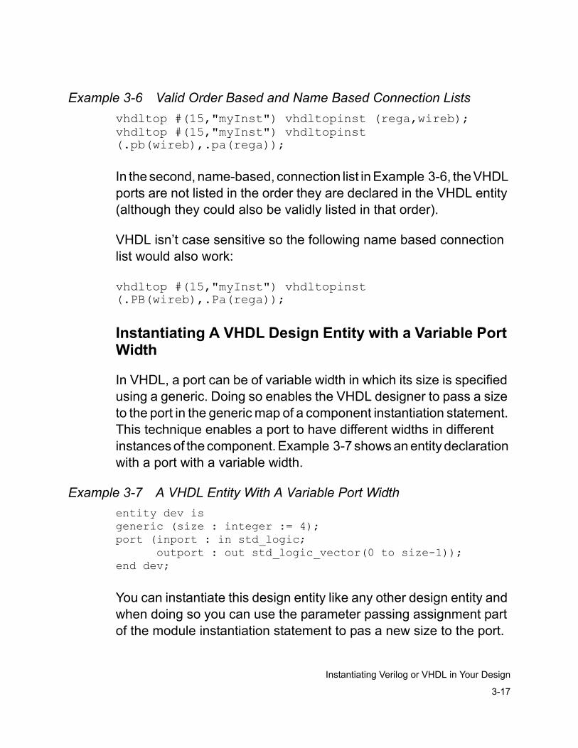
3-17
Instantiating Verilog or VHDL in Your Design
Example 3-6 Valid Order Based and Name Based Connection Listsvhdltop #(15,"myInst") vhdltopinst (rega,wireb);vhdltop #(15,"myInst") vhdltopinst (.pb(wireb),.pa(rega));
In the second, name-based, connection list in Example 3-6, the VHDL ports are not listed in the order they are declared in the VHDL entity (although they could also be validly listed in that order).
VHDL isn’t case sensitive so the following name based connection list would also work:
vhdltop #(15,"myInst") vhdltopinst (.PB(wireb),.Pa(rega));
Instantiating A VHDL Design Entity with a Variable Port Width
In VHDL, a port can be of variable width in which its size is specified using a generic. Doing so enables the VHDL designer to pass a size to the port in the generic map of a component instantiation statement. This technique enables a port to have different widths in different instances of the component. Example 3-7 shows an entity declaration with a port with a variable width.
Example 3-7 A VHDL Entity With A Variable Port Widthentity dev isgeneric (size : integer := 4);port (inport : in std_logic; outport : out std_logic_vector(0 to size-1));end dev;
You can instantiate this design entity like any other design entity and when doing so you can use the parameter passing assignment part of the module instantiation statement to pas a new size to the port.
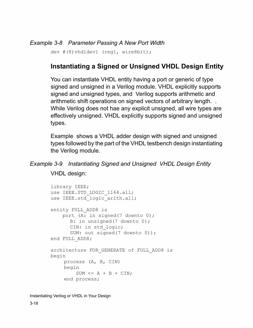
3-18
Instantiating Verilog or VHDL in Your Design
Example 3-8 Parameter Passing A New Port Widthdev #(8)vhdldev1 (reg1, wire8bit);
Instantiating a Signed or Unsigned VHDL Design Entity
You can instantiate VHDL entity having a port or generic of type signed and unsigned in a Verilog module. VHDL explicitly supports signed and unsigned types, and Verilog supports arithmetic and arithmetic shift operations on signed vectors of arbitrary length. . While Verilog does not hae any explicit unsigned, all wire types are effectively unsigned. VHDL explicitly supports signed and unsigned types.
Example shows a VHDL adder design with signed and unsigned types followed by the part of the VHDL testbench design instantiating the Verilog module.
Example 3-9 Instantiating Signed and Unsigned VHDL Design Entity
VHDL design:
library IEEE;use IEEE.STD_LOGIC_1164.all;use IEEE.std_logic_arith.all;
entity FULL_ADD8 is port (A: in signed(7 downto 0);
B: in unsigned(7 downto 0); CIN: in std_logic; SUM: out signed(7 downto 0));
end FULL_ADD8;
architecture FOR_GENERATE of FULL_ADD8 isbegin
process (A, B, CIN)begin SUM <= A + B + CIN;end process;
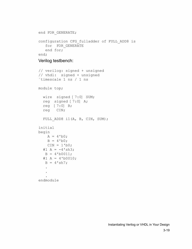
3-19
Instantiating Verilog or VHDL in Your Design
end FOR_GENERATE;
configuration CFG_fulladder of FULL_ADD8 is for FOR_GENERATE end for;end;
Verilog testbench:
// verilog: signed + unsigned// vhdl: signed + unsigned`timescale 1 ns / 1 ns
module top;
wire signed [7:0] SUM; reg signed [7:0] A; reg [7:0] B; reg CIN;
FULL_ADD8 i1(A, B, CIN, SUM);
initialbegin A = 4'b0; B = 4'b0; CIN = 1'b0; #1 A = -4'sh3; B = 4'b0011; #1 A = 4'b0010; B = 4'sh7; . . .endmodule
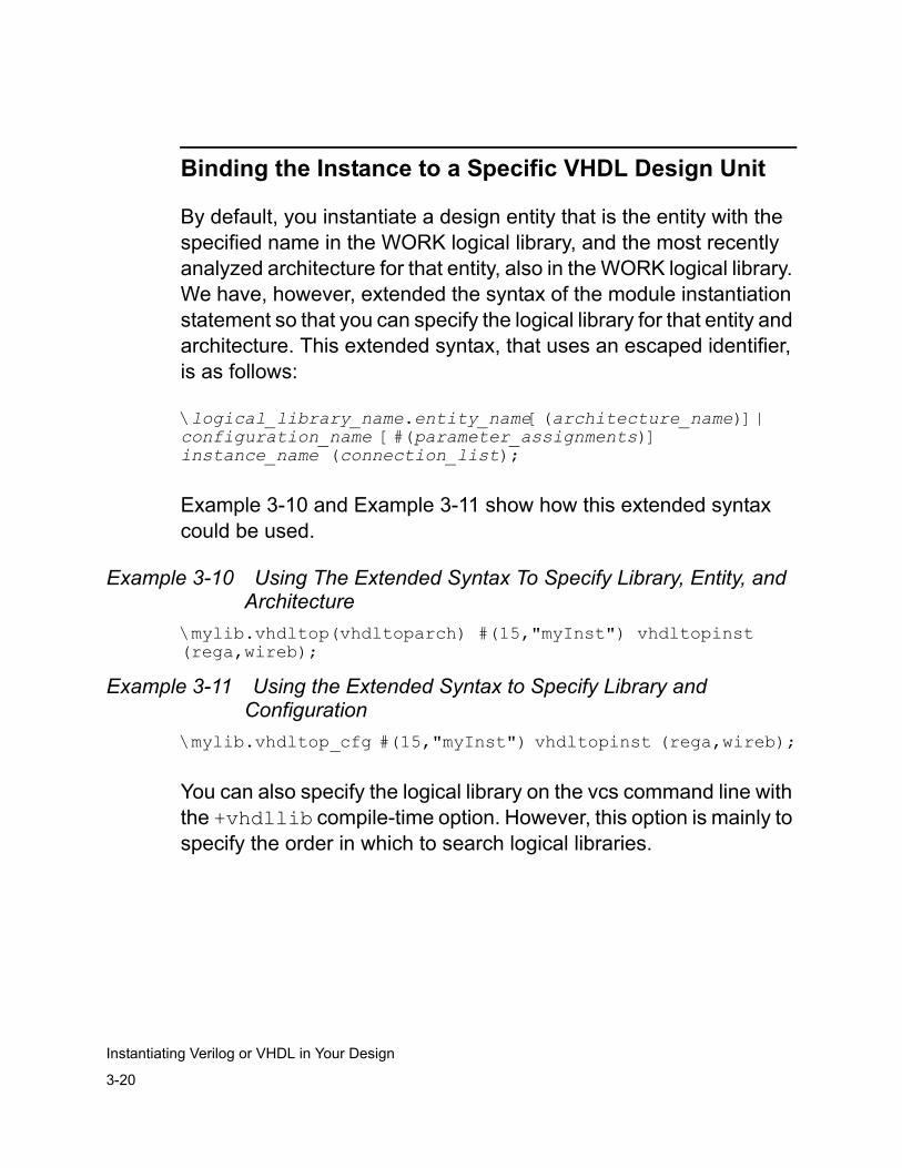
3-20
Instantiating Verilog or VHDL in Your Design
Binding the Instance to a Specific VHDL Design Unit
By default, you instantiate a design entity that is the entity with the specified name in the WORK logical library, and the most recently analyzed architecture for that entity, also in the WORK logical library. We have, however, extended the syntax of the module instantiation statement so that you can specify the logical library for that entity and architecture. This extended syntax, that uses an escaped identifier, is as follows:
\logical_library_name.entity_name[(architecture_name)]| configuration_name [#(parameter_assignments)] instance_name (connection_list);
Example 3-10 and Example 3-11 show how this extended syntax could be used.
Example 3-10 Using The Extended Syntax To Specify Library, Entity, and Architecture
\mylib.vhdltop(vhdltoparch) #(15,"myInst") vhdltopinst (rega,wireb);
Example 3-11 Using the Extended Syntax to Specify Library and Configuration
\mylib.vhdltop_cfg #(15,"myInst") vhdltopinst (rega,wireb);
You can also specify the logical library on the vcs command line with the +vhdllib compile-time option. However, this option is mainly to specify the order in which to search logical libraries.
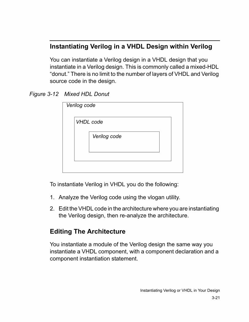
3-21
Instantiating Verilog or VHDL in Your Design
Instantiating Verilog in a VHDL Design within Verilog
You can instantiate a Verilog design in a VHDL design that you instantiate in a Verilog design. This is commonly called a mixed-HDL “donut.” There is no limit to the number of layers of VHDL and Verilog source code in the design.
Figure 3-12 Mixed HDL Donut
To instantiate Verilog in VHDL you do the following:
1. Analyze the Verilog code using the vlogan utility.
2. Edit the VHDL code in the architecture where you are instantiating the Verilog design, then re-analyze the architecture.
Editing The Architecture
You instantiate a module of the Verilog design the same way you instantiate a VHDL component, with a component declaration and a component instantiation statement.
Verilog code
VHDL code
Verilog code
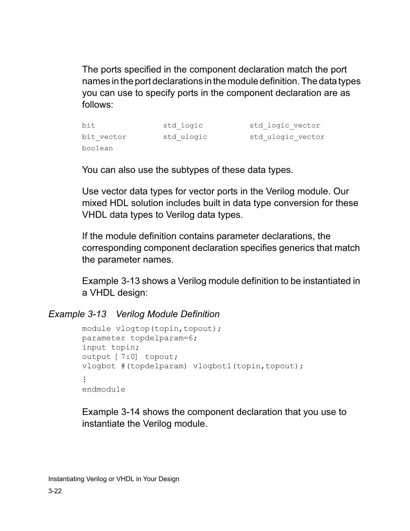
3-22
Instantiating Verilog or VHDL in Your Design
The ports specified in the component declaration match the port names in the port declarations in the module definition. The data types you can use to specify ports in the component declaration are as follows:
You can also use the subtypes of these data types.
Use vector data types for vector ports in the Verilog module. Our mixed HDL solution includes built in data type conversion for these VHDL data types to Verilog data types.
If the module definition contains parameter declarations, the corresponding component declaration specifies generics that match the parameter names.
Example 3-13 shows a Verilog module definition to be instantiated in a VHDL design:
Example 3-13 Verilog Module Definitionmodule vlogtop(topin,topout);parameter topdelparam=6;input topin;output [7:0] topout;vlogbot #(topdelparam) vlogbot1(topin,topout);...endmodule
Example 3-14 shows the component declaration that you use to instantiate the Verilog module.
bit std_logic std_logic_vector
bit_vector std_ulogic std_ulogic_vector
boolean
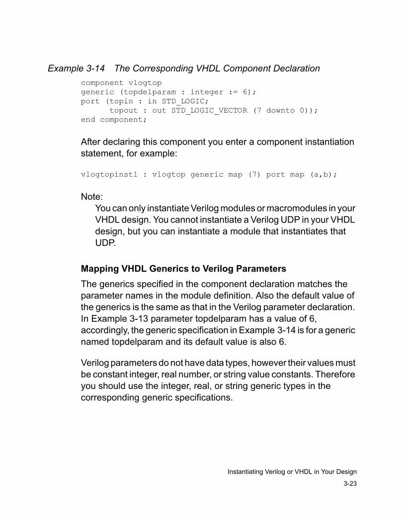
3-23
Instantiating Verilog or VHDL in Your Design
Example 3-14 The Corresponding VHDL Component Declarationcomponent vlogtopgeneric (topdelparam : integer := 6);port (topin : in STD_LOGIC; topout : out STD_LOGIC_VECTOR (7 downto 0));end component;
After declaring this component you enter a component instantiation statement, for example:
vlogtopinst1 : vlogtop generic map (7) port map (a,b);
Note: You can only instantiate Verilog modules or macromodules in your VHDL design. You cannot instantiate a Verilog UDP in your VHDL design, but you can instantiate a module that instantiates that UDP.
Mapping VHDL Generics to Verilog ParametersThe generics specified in the component declaration matches the parameter names in the module definition. Also the default value of the generics is the same as that in the Verilog parameter declaration. In Example 3-13 parameter topdelparam has a value of 6, accordingly, the generic specification in Example 3-14 is for a generic named topdelparam and its default value is also 6.
Verilog parameters do not have data types, however their values must be constant integer, real number, or string value constants. Therefore you should use the integer, real, or string generic types in the corresponding generic specifications.
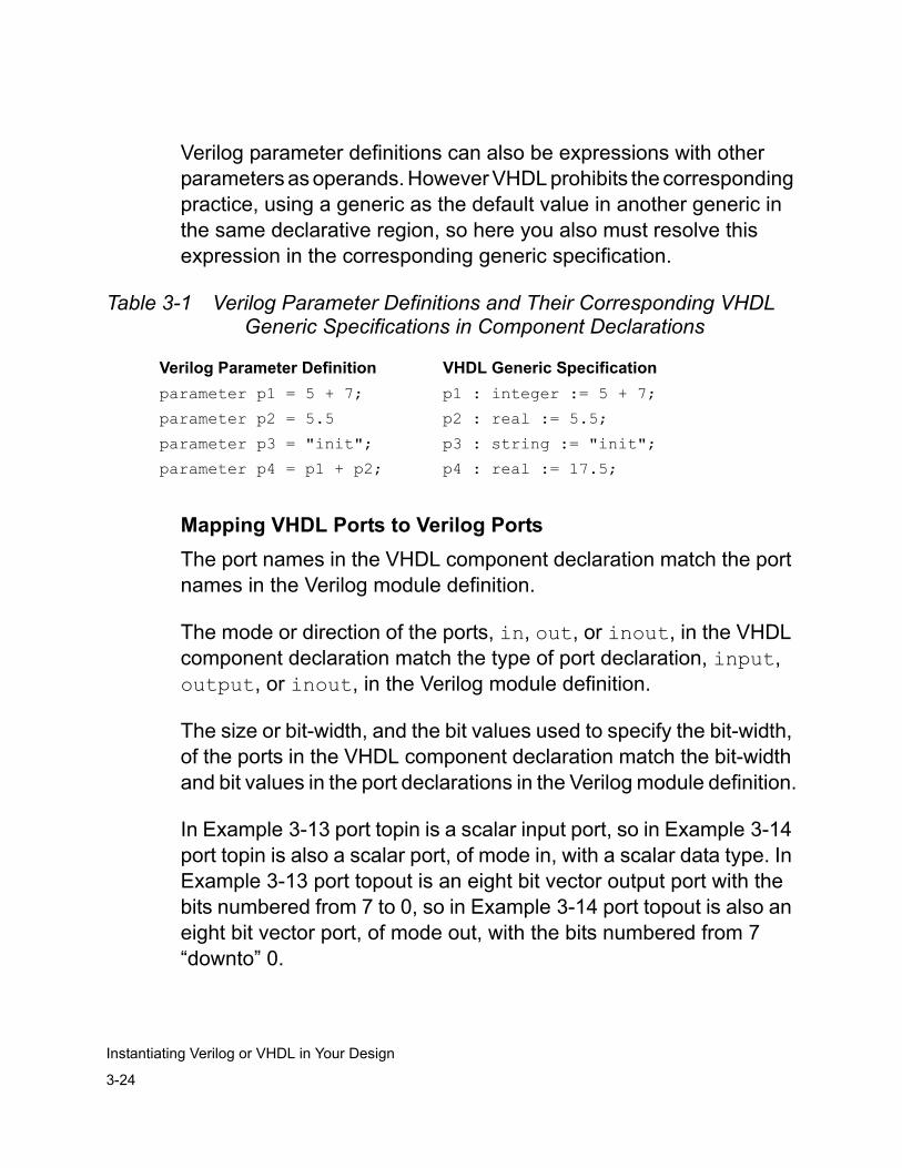
3-24
Instantiating Verilog or VHDL in Your Design
Verilog parameter definitions can also be expressions with other parameters as operands. However VHDL prohibits the corresponding practice, using a generic as the default value in another generic in the same declarative region, so here you also must resolve this expression in the corresponding generic specification.
Table 3-1 Verilog Parameter Definitions and Their Corresponding VHDL Generic Specifications in Component Declarations
Mapping VHDL Ports to Verilog PortsThe port names in the VHDL component declaration match the port names in the Verilog module definition.
The mode or direction of the ports, in, out, or inout, in the VHDL component declaration match the type of port declaration, input, output, or inout, in the Verilog module definition.
The size or bit-width, and the bit values used to specify the bit-width, of the ports in the VHDL component declaration match the bit-width and bit values in the port declarations in the Verilog module definition.
In Example 3-13 port topin is a scalar input port, so in Example 3-14 port topin is also a scalar port, of mode in, with a scalar data type. In Example 3-13 port topout is an eight bit vector output port with the bits numbered from 7 to 0, so in Example 3-14 port topout is also an eight bit vector port, of mode out, with the bits numbered from 7 “downto” 0.
Verilog Parameter Definition VHDL Generic Specificationparameter p1 = 5 + 7; p1 : integer := 5 + 7;
parameter p2 = 5.5 p2 : real := 5.5;
parameter p3 = "init"; p3 : string := "init";
parameter p4 = p1 + p2; p4 : real := 17.5;
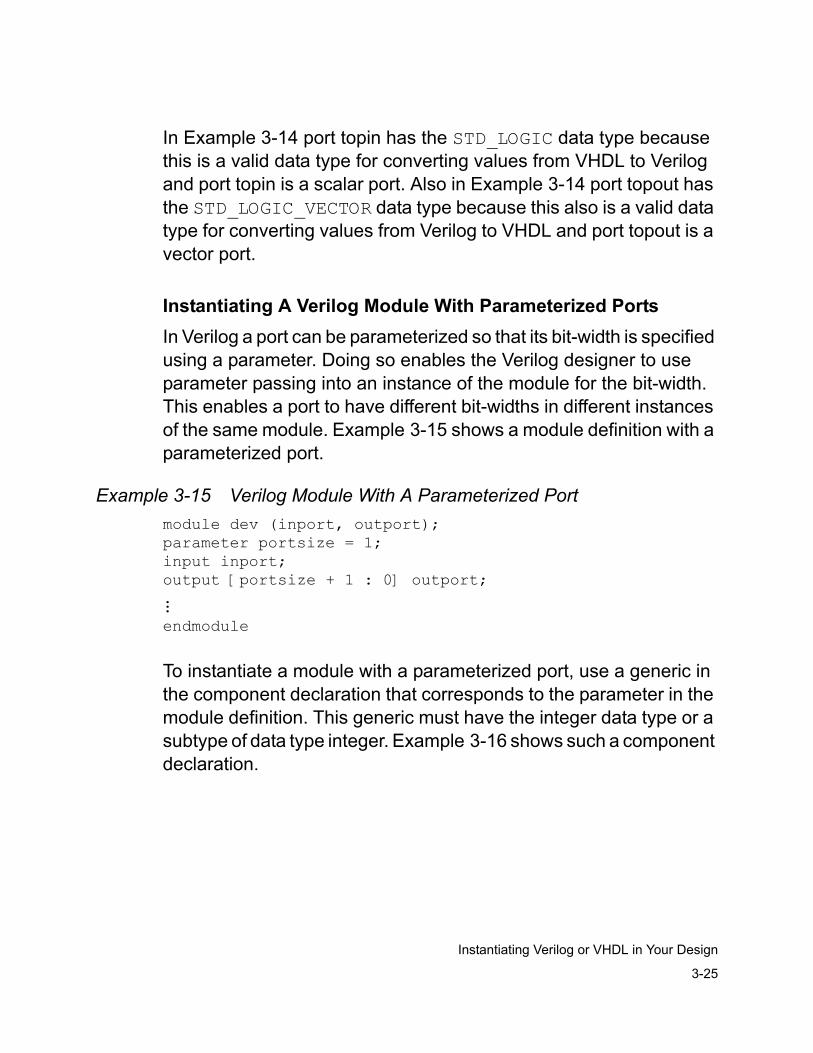
3-25
Instantiating Verilog or VHDL in Your Design
In Example 3-14 port topin has the STD_LOGIC data type because this is a valid data type for converting values from VHDL to Verilog and port topin is a scalar port. Also in Example 3-14 port topout has the STD_LOGIC_VECTOR data type because this also is a valid data type for converting values from Verilog to VHDL and port topout is a vector port.
Instantiating A Verilog Module With Parameterized PortsIn Verilog a port can be parameterized so that its bit-width is specified using a parameter. Doing so enables the Verilog designer to use parameter passing into an instance of the module for the bit-width. This enables a port to have different bit-widths in different instances of the same module. Example 3-15 shows a module definition with a parameterized port.
Example 3-15 Verilog Module With A Parameterized Portmodule dev (inport, outport);parameter portsize = 1;input inport;output [portsize + 1 : 0] outport;...endmodule
To instantiate a module with a parameterized port, use a generic in the component declaration that corresponds to the parameter in the module definition. This generic must have the integer data type or a subtype of data type integer. Example 3-16 shows such a component declaration.
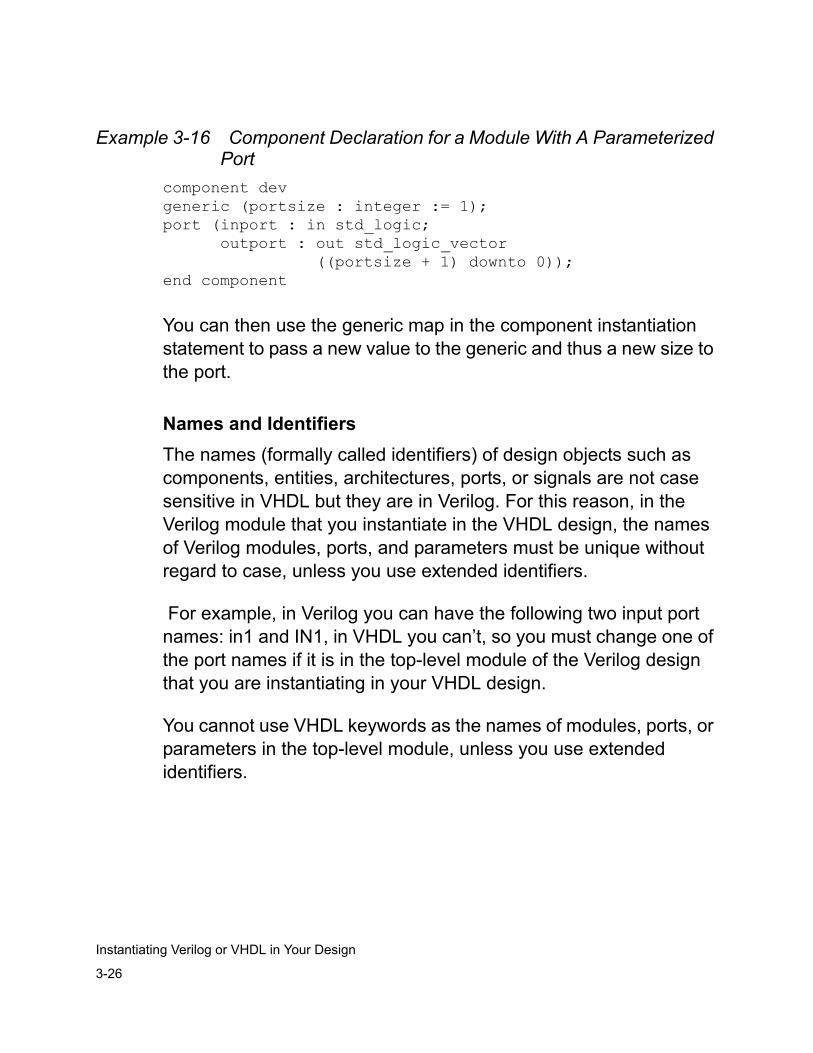
3-26
Instantiating Verilog or VHDL in Your Design
Example 3-16 Component Declaration for a Module With A Parameterized Port
component devgeneric (portsize : integer := 1);port (inport : in std_logic; outport : out std_logic_vector ((portsize + 1) downto 0));end component
You can then use the generic map in the component instantiation statement to pass a new value to the generic and thus a new size to the port.
Names and IdentifiersThe names (formally called identifiers) of design objects such as components, entities, architectures, ports, or signals are not case sensitive in VHDL but they are in Verilog. For this reason, in the Verilog module that you instantiate in the VHDL design, the names of Verilog modules, ports, and parameters must be unique without regard to case, unless you use extended identifiers.
For example, in Verilog you can have the following two input port names: in1 and IN1, in VHDL you can’t, so you must change one of the port names if it is in the top-level module of the Verilog design that you are instantiating in your VHDL design.
You cannot use VHDL keywords as the names of modules, ports, or parameters in the top-level module, unless you use extended identifiers.
3-27
Instantiating Verilog or VHDL in Your Design
You must follow the rules for VHDL identifiers in the names of modules, ports, or parameters in the top-level module. Valid VHDL identifiers consist of upper or lower case letters, numbers, and the underscore, the first character must be a letter, and the last character cannot be the underscore _, unless you use extended identifiers.
Using Extended IdentifiersYou can use extended identifiers (similar to Verilog escaped identifiers) to circumvent the rules for VHDL identifiers, for example:
• You can have ports \in1\ and \IN1\ in the component declaration.
• You can have an entity named \component\.
• You can begin a name with a number and end with an underscore, such as an architecture named \1comparch_\.
Module Header Port List RestrictionsThe port list in the module header for the instantiated module cannot contain either of the following:
•Unconnected ports
An unconnected port is an empty space between commas in the port connection list, for example:
module vlogtop (portia, ,portib);
•Jumpered ports
A jumpered port is a port that appears more than once in the port list, for example:
module vlogtop (portia, portia);

3-28
Instantiating Verilog or VHDL in Your Design
4-1
Analyzing Your Design
4Analyzing Your Design 3
This chapter describes the analysis phase of mixed-HDL simulation.
It is important to note that the analysis phase can be affected if you are instantiating either Verilog in a VHDL design, or VHDL code in a Verilog design. If this is the case, you should also refer to “Instantiating Verilog or VHDL in Your Design” in Chapter 3.This chapter contains the following sections:
• "Introduction to Analysis" on page 4-2
• "Analyzing The VHDL Portion Of A Design" on page 4-3
• "Common vhdlan Analysis Options" on page 4-15
• "Analyzing The Verilog Portion Of A Design" on page 4-29
4-2
Analyzing Your Design
Introduction to Analysis
The VCS MX Analyzer analyzes source files, produces intermediate files for elaboration and saves these files in the design library.
VCS MX uses the vhdlan utility to analyze VHDL-only designs, and the VHDL portion of VHDL-top or Verilog-top designs. Similarly, VCS MX uses the vlogan utility to analyze Verilog-only designs, and the Verilog portion of Verilog-top or VHDL-top designs.
The recommended flow for a mixed language design is to first analyze all of your Verilog source code using the vlogan command and then analyze all of your VHDL source code using vhdlan.
For details on the analysis process as it applies to a Verilog design instantiated within a VHDL design, see “Instantiating a Verilog Design in a VHDL Design” on page 4-2. For details on the analysis process as it applies to a VHDL design instantiated within a Verilog design, see “Instantiating a VHDL Design within a Verilog Design” on page 4-12.
Creating a Design Library
In the SYNOPSYS_SIM.SETUP file, you can create entries that map the library logical name WORK to a design library name, and the design library name to a host system directory. The VCS MX Analyzer checks the entries in the setup file to determine where to place the analyzed design library units.
4-3
Analyzing Your Design
For more information about design library mapping in the setup file, see “Creating the Setup File” on page 1-4. You can use the -work option with the vhdlan command or vlogan command to analyze VHDL or Verilog code into different logical libraries. For more information on using the -work option with the vhdlan command’ see "Specifying a Design Library" on page 4-19.
During analysis, the VCS MX Analyzer places output files in the physical directory, which is mapped to the logical library. The specific set of output files that the Analyzer creates, depends on the settings in the setup file, and the switches you use for analysis.
Analyzing The VHDL Portion Of A Design
For analyzing VHDL source files in a VHDL or mixed-HDL design, you need to use the vhdlan utility. This utility can be used with different options to analyze the source files for different types of simulation. For more information about different vhdlan options, see “Common vhdlan Analysis Options” on page 4-15. You can also use utilities such as simdepends and simcompiled to track dependencies on a source file and determine the list of options that were used to analyze a module. For more information about these utilities, see “Maintaining VHDL Designs” on page 4-4.
Using vhdlan
The vhdlan utility performs the analysis process for VHDL-only designs, and the VHDL portion of VHDL-top designs or Verilog-top designs. The syntax for the vhdlan command is as follows:
vhdlan [options] filename_list
4-4
Analyzing Your Design
Use filename_list to list the names of one or more files you want to analyze. A file extension is optional; if none is given, VHDL Analyzer assumes it to be .vhd.
For example, to analyze the mux.vhd file, enter the following:
% vhdlan mux.vhd
Note:The maximum identifier name length is 250 for package, package body and configuration names. The combined length of an entity name plus architecture name must not exceed 250 characters as well. All other VHDL identifier names and string literals do not have a length limitation.
For complete syntax details on the vhdlan command, see “vhdlan Utility” on page 3-2 of the VCS MX Reference Guide.
Maintaining VHDL Designs
When you modify the VHDL source code for a design unit, you must analyze the source file again so that the intermediate (.sim, .o, and .mra) files used by the simulator reflect the current information in the source files. You must also reanalyze any VHDL source files that contain design units that instantiate the modified design unit.
In a large design, these source file dependencies can become difficult to track manually. VCS MX provides utilities to help you do the following:
• Create a file that contains a list of target dependencies for a design unit.
• Reanalyze a source file, and automatically reanalyze the source files for all design units that are affected by that source file.
4-5
Analyzing Your Design
• Determine the options you used when you analyzed a module for simulation.
When maintaining your design, you cannot run a simulation using a design library created with a version of VHDL Analyzer that does not match the version of the simulator you are using. The binary format of the intermediate files can change from one software release to another. Therefore, you need to reanalyze all your design library files after you install a new release of the simulation software.
Creating a Dependency List File
Use the simdepends utility to create a file (makefile) that simplifies the task of reanalyzing your source files. The simdepends utility has the following functions:
• Identifies intermediate files for design units that refer to the modified design unit.
• Creates a list of target dependencies for source files that must be reanalyzed when you edit a source file. You can then use this list as input to the UNIX make utility to reanalyze all the files that must be reanalyzed.
• Records the options you used when you analyzed your source files. When you reanalyze a source file with the make utility, VHDL Analyzer uses the same options as it did the last time it analyzed that file.
4-6
Analyzing Your Design
Using simdepends
Figure 4-1 illustrates how to use the simdepends utility. The process involves the following steps:
1. Analyze your design files with vhdlan.
2. Run simdepends to create a list of dependencies. Redirect the output to a file (makefile).
3. Compile your design with scs.
4. Simulate and debug your design with VCS MX.
5. Edit your VHDL source files.
6. Use the UNIX make utility to reanalyze the edited VHDL source files and all VHDL source files that depend on them.
You have to run simdepends again only if you add new design units or library units to the simulation or if you change a path to these units.
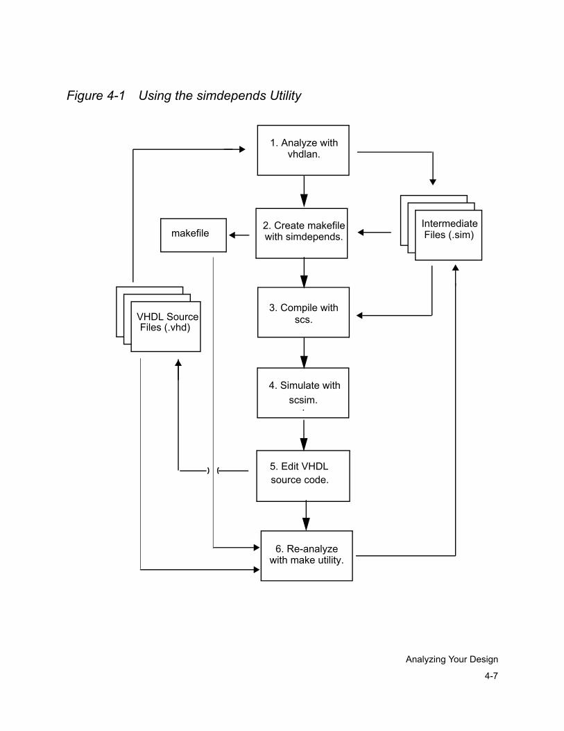
4-7
Analyzing Your Design
Figure 4-1 Using the simdepends Utility
VHDL SourceFiles (.vhd)
IntermediateFiles (.sim)
vhdlan.
2. Create makefilewith simdepends.makefile
4. Simulate with
.
5. Edit VHDL source code.
6. Re-analyzewith make utility.
1. Analyze with
scsim.
3. Compile withscs.
4-8
Analyzing Your Design
Invoking simdepends
Run simdepends immediately after analyzing the new design source files.
To create a dependency list for a single design unit, use the following syntax:
% simdepends [options] design_unit
To create a dependency list for more than one design unit, use the -u option to specify additional design units.
% simdepends [options] design_unit -u design_unit
You can use more than one instance of -u design_unit.
Specifying the Design UnitThe design unit you specify must be the name of the top-level design unit for the simulation, for example, the testbench configuration name. If you do this, simdepends enters all the intermediate files for the simulation as target dependencies.
The design unit can be an entity, package, or configuration. To specify an entity, use the following syntax:
[libname.]entity__archname
libname and archname are optional. libname is a library logical name that is mapped to a design library in the setup file. If you do not provide libname, simdepends uses the library mapped to the WORK variable. If you do not provide archname, simdepends uses the most recently analyzed architecture.
4-9
Analyzing Your Design
If the design_unit is a package or configuration, do not use archname.
Specifying an Output FileInvoke simdepends with the -o filename option to send the output to a file. The output file can have any name; however, it is most convenient to use the name makefile, the default name for the make utility. For example, to write the dependency list for the design unit comparator to the file makefile, enter the following:
% simdepends -o makefile comparator
The -o filename option is the most commonly used simdepends option.
For complete syntax information on the simdepends utility, see “simdepends Utility” on page 3-17 of the VCS MX Reference Guide.
simdepends Example
The following example shows the source files for a simple design used for analysis, the output files produced for mixed event and cycle simulation, and the use of the simdepends utility to create a makefile.
Source FilesThis example uses the following VHDL source files, residing in a single directory:
• The x.vhd file, which contains
package P is end P;
• The y.vhd file, which contains
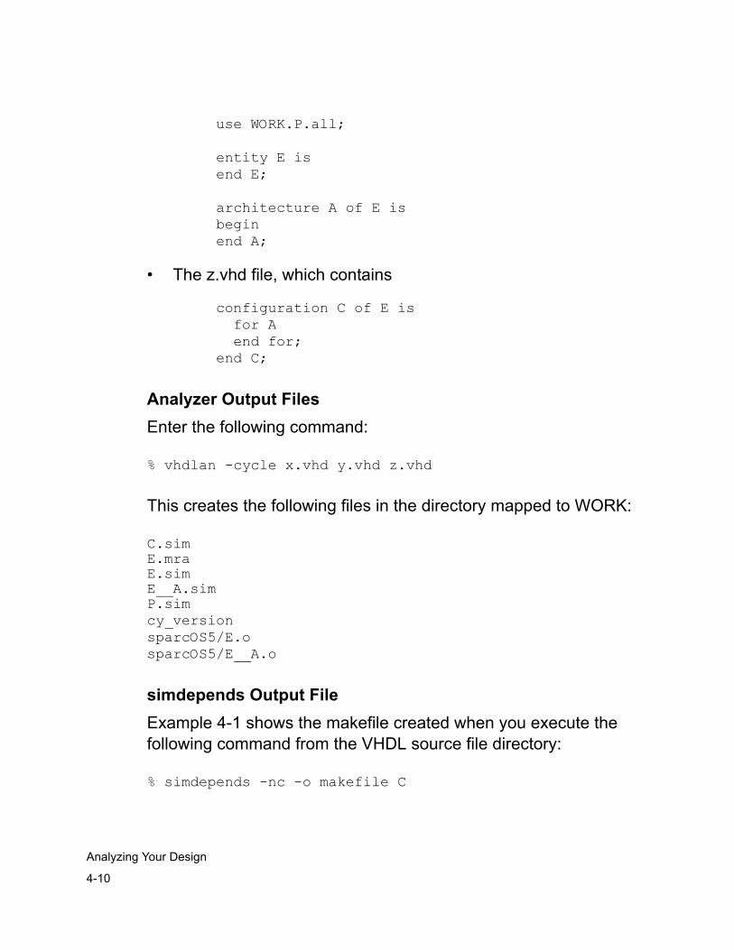
4-10
Analyzing Your Design
use WORK.P.all;
entity E is end E;
architecture A of E is begin end A;
• The z.vhd file, which contains
configuration C of E is for A end for; end C;
Analyzer Output FilesEnter the following command:
% vhdlan -cycle x.vhd y.vhd z.vhd
This creates the following files in the directory mapped to WORK:
C.simE.mraE.sim E__A.simP.simcy_versionsparcOS5/E.osparcOS5/E__A.o
simdepends Output FileExample 4-1 shows the makefile created when you execute the following command from the VHDL source file directory:
% simdepends -nc -o makefile C
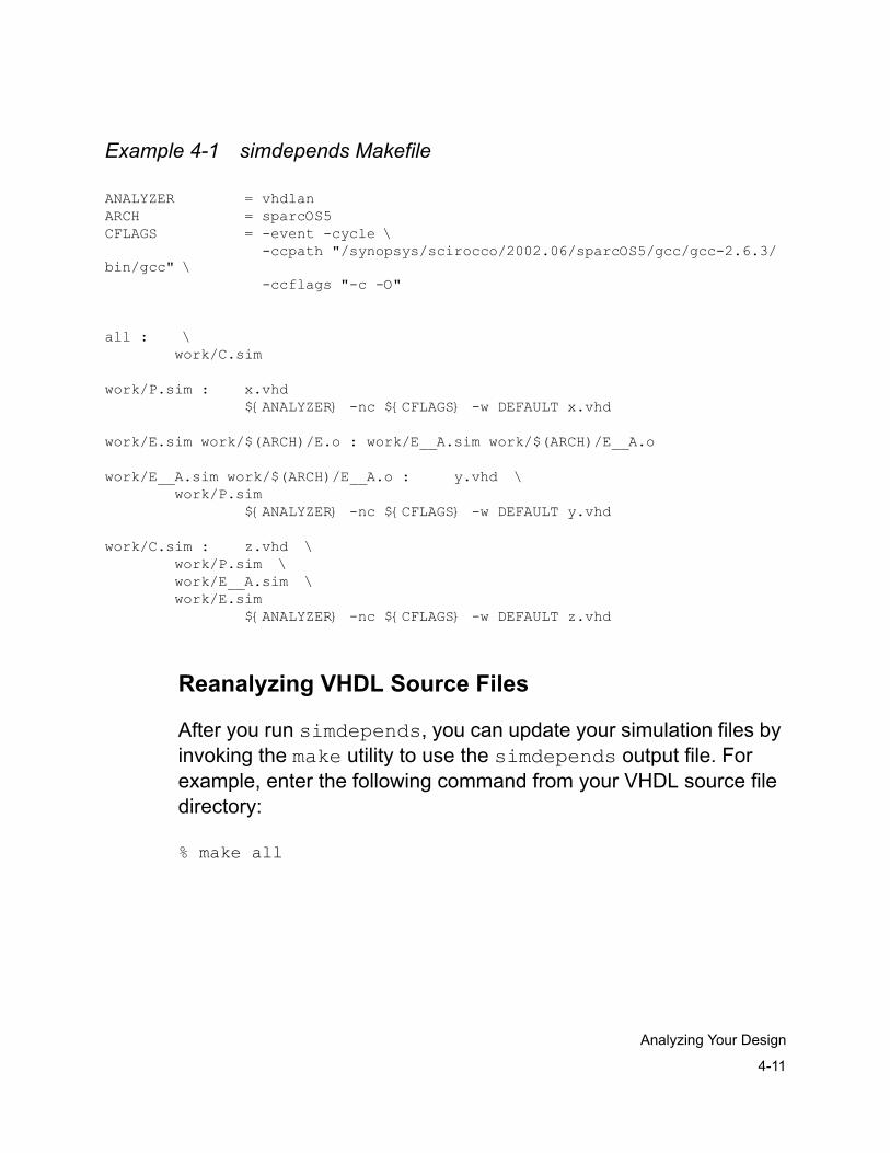
4-11
Analyzing Your Design
Example 4-1 simdepends Makefile
ANALYZER = vhdlanARCH = sparcOS5CFLAGS = -event -cycle \ -ccpath "/synopsys/scirocco/2002.06/sparcOS5/gcc/gcc-2.6.3/bin/gcc" \ -ccflags "-c -O" all : \ work/C.sim work/P.sim : x.vhd ${ANALYZER} -nc ${CFLAGS} -w DEFAULT x.vhd work/E.sim work/$(ARCH)/E.o : work/E__A.sim work/$(ARCH)/E__A.o work/E__A.sim work/$(ARCH)/E__A.o : y.vhd \ work/P.sim ${ANALYZER} -nc ${CFLAGS} -w DEFAULT y.vhd work/C.sim : z.vhd \ work/P.sim \ work/E__A.sim \ work/E.sim ${ANALYZER} -nc ${CFLAGS} -w DEFAULT z.vhd
Reanalyzing VHDL Source Files
After you run simdepends, you can update your simulation files by invoking the make utility to use the simdepends output file. For example, enter the following command from your VHDL source file directory:
% make all
4-12
Analyzing Your Design
If a design unit intermediate file is out of date, make automatically reanalyzes the source file and the source files for all design units that refer to that design unit. When make finishes, all intermediate files used in the simulation are up to date, and the new simulation is ready to run.
Determining Analyzer Options
The simcompiled utility provides compiled simulation information for a design unit. If you analyze a design unit for simulation and later want to know which analyzer options you used, invoke simcompiled on the design unit.
Invoking simcompiled
The simcompiled command syntax is:
% simcompiled [options] design_unit [-u design_unit]
You specify the design unit the same way you do for the simdepends utility (see the “Specifying the Design Unit” section). A second design unit can be specified by using the -u option.
To redirect the simcompiled output to a file, use the -o makefile option. For example, enter the command:
% simcompiled -o compfile comparator
This generates a list of options used for compilation of the design unit comparator and writes it to the file compfile.
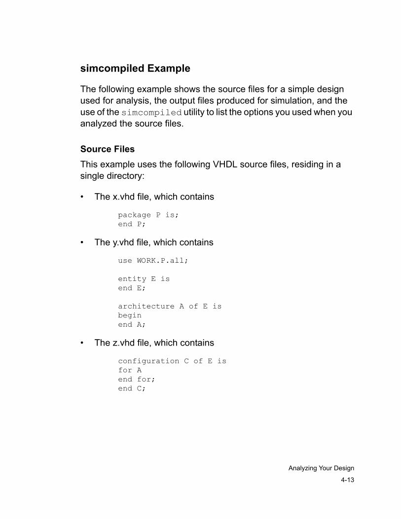
4-13
Analyzing Your Design
simcompiled Example
The following example shows the source files for a simple design used for analysis, the output files produced for simulation, and the use of the simcompiled utility to list the options you used when you analyzed the source files.
Source FilesThis example uses the following VHDL source files, residing in a single directory:
• The x.vhd file, which contains
package P is; end P;
• The y.vhd file, which contains
use WORK.P.all;
entity E is end E;
architecture A of E is begin end A;
• The z.vhd file, which contains
configuration C of E is for A end for; end C;

4-14
Analyzing Your Design
Analyzer Output FilesEnter the following command:
vhdlan -cycle x.vhd y.vhd z.vhd
This generates debuggable and compiled event code and cycle code, and creates the following files in the directory mapped to WORK:
C.simE.mraE.simE__A.simP.simcy_versionsparcOS5/E.osparcOS5/E__A.o
simcompiled Output FileExample 4-2 shows the output file created when you execute the following command from the VHDL source file directory:
% simcompiled -nc -o compfile C
Example 4-2 simcompiled Output FileFlags common to ALL design units: -event -cycle -ccpath "/synopsys/scirocco/2002.06/sparcOS5/gcc/gcc-2.6.3/bin/gcc" -ccflags "-c -O"
simcompiled Utility
For complete details on the syntax for the simcompiled utility, see “simcompiled Utility” on page 3-19 of the VCS MX Reference Guide.
4-15
Analyzing Your Design
Common vhdlan Analysis Options
Some of the more commonly used vhdlan options enable the following:
• "Analyzing for Simulation Technology" on page 4-15
• "Modifying Compiled Event Simulation Analysis" on page 4-17
• "Specifying a Design Library" on page 4-19
• "Checking Synthesis Policy" on page 4-20
• "Creating a List File" on page 4-22
• "The analyzer names the list file filename.lis and places it in the same directory as the VHDL source file. Relaxing VHDL LRM Conformance" on page 4-23
• "Analyzing for Functional VITAL Simulation Mode" on page 4-26
• "Smart Analysis" on page 4-28
Analyzing for Simulation Technology
You can analyze your files for debuggable event-driven, compiled event-driven, or compiled cycle-based simulation. Table 4-1 summarizes the various codes the analyzer generates based on the options you specify, either on the command line with the vhdlan command or with the DEFAULT_ANALYZE_MODE setup variable.
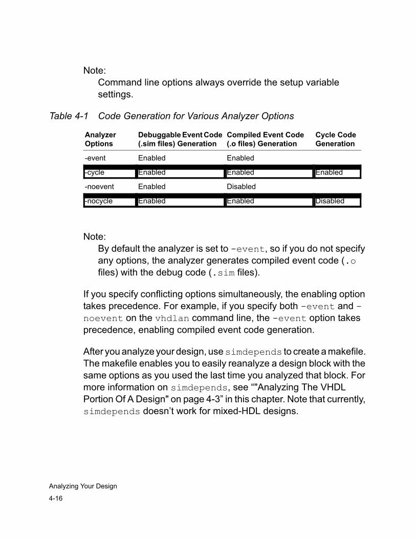
4-16
Analyzing Your Design
Note:Command line options always override the setup variable settings.
Table 4-1 Code Generation for Various Analyzer Options
Note:By default the analyzer is set to -event, so if you do not specify any options, the analyzer generates compiled event code (.o files) with the debug code (.sim files).
If you specify conflicting options simultaneously, the enabling option takes precedence. For example, if you specify both -event and -noevent on the vhdlan command line, the -event option takes precedence, enabling compiled event code generation.
After you analyze your design, use simdepends to create a makefile. The makefile enables you to easily reanalyze a design block with the same options as you used the last time you analyzed that block. For more information on simdepends, see “"Analyzing The VHDL Portion Of A Design" on page 4-3” in this chapter. Note that currently, simdepends doesn’t work for mixed-HDL designs.
Analyzer Options
Debuggable Event Code (.sim files) Generation
Compiled Event Code (.o files) Generation
Cycle Code Generation
-event Enabled Enabled
-cycle Enabled Enabled Enabled
-noevent Enabled Disabled
-nocycle Enabled Enabled Disabled
4-17
Analyzing Your Design
Analyzing for Compiled Cycle-based SimulationFor mixed event, cycle mode and full cycle mode simulation, you need to invoke VHDL Analyzer with the -cycle option to perform additional checks for cycle based policy violations when it analyzes your VHDL design files. It checks the VHDL design file against the VHDL cycle-based subset. If a violation is found, an error is generated. For information about the VHDL cycle based subset, see the VHDL Simulation Coding and Modeling Style Guide.
Modifying Compiled Event Simulation Analysis
If you are analyzing a design block for compiled event simulation, you can use vhdlan command line modifiers to:
• Optimize compiled code
• Pass options to the compiler
Optimizing Compiled Code
By default, VCS MX Analyzer generates optimized compiled code for running the event simulation. This optimized compiled code enhances VCS MX performance.
Typically when you are developing your design and are still in the debugging phase, you want to enforce more checks on the VHDL source of your design. VHDL Analyzer can perform additional VHDL checks for:
• Arithmetic overflow
• Constraint checks
• Array size compatibility at assignment
4-18
Analyzing Your Design
• Subscripts out of bounds
• Negative exponents to integer
To switch off optimizations, and make these checks available to you, use the following option:
-no_optGenerates updated code which contains embedded run-time options.
Caution!You should run your design at least once with the checks enabled, by using -no_opt. Otherwise, if a VHDL error occurs, and you have disabled checking, you can get erroneous results or cause the simulator to fail in an unpredictable way.
Passing Options to the C Compiler
You can use the -ccflags "option_string" to pass options to the C compiler. Table 4-2 shows the default option string and optimize option for each platform.
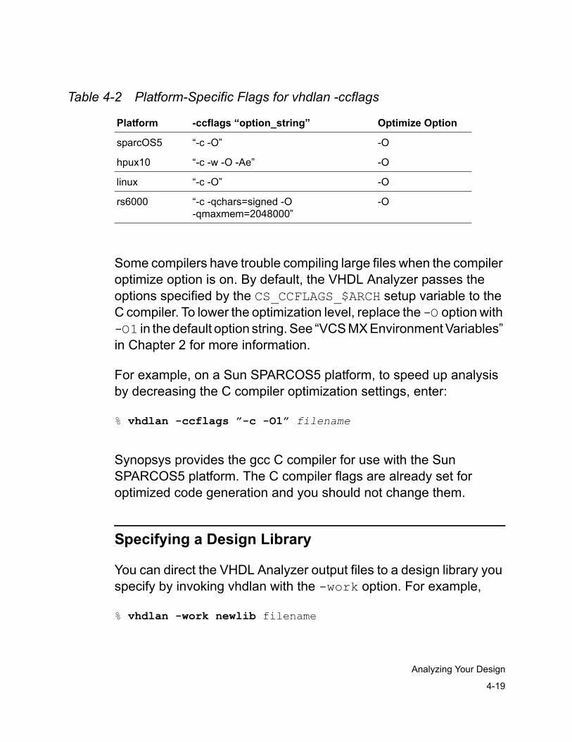
4-19
Analyzing Your Design
Table 4-2 Platform-Specific Flags for vhdlan -ccflags
Some compilers have trouble compiling large files when the compiler optimize option is on. By default, the VHDL Analyzer passes the options specified by the CS_CCFLAGS_$ARCH setup variable to the C compiler. To lower the optimization level, replace the -O option with -O1 in the default option string. See “VCS MX Environment Variables” in Chapter 2 for more information.
For example, on a Sun SPARCOS5 platform, to speed up analysis by decreasing the C compiler optimization settings, enter:
% vhdlan -ccflags ”-c -O1” filename
Synopsys provides the gcc C compiler for use with the Sun SPARCOS5 platform. The C compiler flags are already set for optimized code generation and you should not change them.
Specifying a Design Library
You can direct the VHDL Analyzer output files to a design library you specify by invoking vhdlan with the -work option. For example,
% vhdlan -work newlib filename
Platform -ccflags “option_string” Optimize Option
sparcOS5 “-c -O” -O
hpux10 “-c -w -O -Ae” -O
linux “-c -O” -O
rs6000 “-c -qchars=signed -O -qmaxmem=2048000”
-O
4-20
Analyzing Your Design
This directs the output files to the newlib design library.
The SYNOPSYS_SIM.SETUP file must contain an entry that maps the design library name to a host system directory. For example,
newlib : /home/joe/lib2
Note: Using the -work newlib option has the same result as the WORK > newlib entry in the SYNOPSYS_SIM.SETUP file.
You can also specify the physical path name of the logical design library with the -work option of vhdlan. For example, if the library mapping in SYNOPSYS_SIM.SETUP file is as follows:
LIB1 = /abc/def/ghi/work
To analyze a file.vhd into logical library LIB1, you can use the following command:
% vhdlan -work LIB1 file.vhd
With the mapping in SYNOPSYS_SIM.SETUP, it is clear that the logical library is LIB1. So any source that has "library LIB1; use LIB1.all;" statements for instantiated components (which were compiled in /abc/def/ghi/work) gets analyzed without errors.
Checking Synthesis Policy
You can invoke VHDL Analyzer to perform synthesis policy checking (SPC) when it analyzes your VHDL design files. SPC checks the VHDL design file against the VHDL subset supported by Synopsys synthesis tools.
4-21
Analyzing Your Design
Additionally, the -spc option creates post analysis synthesis files with a .syn suffix. Therefore, you only need to analyze your files once for both synthesis and simulation as long as you use the same version for both. You must use the -spc option to analyze all the design files on which the file you are analyzing depends.
The following example shows how to use the -spc option:
% vhdlan -spc filename
Note: You need have a Synopsys Design Compiler installation and license to use the -spc option.

4-22
Analyzing Your Design
Creating a List File
An Analyzer list file contains the following details about all the source files that it analyzes:
• Name of the source file
• Time that the .lis file was created
• VHDL source listing
• Names of the analyzed units
• Warning or error messages generated during the analysis
Use the -list option to create an Analyzer list file. For example, the command:
% vhdlan -list filename
Creates the following list file:
-- Synopsys 1076 VHDL Analyzer Version 2002.06 -- Apr 14, 2002---- Copyright (c) 1990-2000 by Synopsys, Inc.-- ALL RIGHTS RESERVED-- This program is proprietary and confidential information-- of Synopsys, Inc. and may be used and disclosed only as-- authorized in a license agreement controlling such use-- and disclosure.---- Source File: zero.vhd-- Sat Apr 15 21:28:23 2001
1 library IEEE; 2 use IEEE.std_logic_1164.all; 3 use IEEE.std_logic_arith.all; 4 5 entity ZERO is
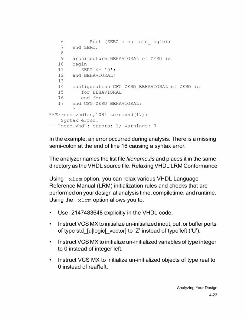
4-23
Analyzing Your Design
6 Port (ZERO : out std_logic); 7 end ZERO; 8 9 architecture BEHAVIORAL of ZERO is 10 begin 11 ZERO <= '0'; 12 end BEHAVIORAL; 13 14 configuration CFG_ZERO_BEHAVIORAL of ZERO is 15 for BEHAVIORAL 16 end for 17 end CFG_ZERO_BEHAVIORAL; ^**Error: vhdlan,1081 zero.vhd(17): Syntax error.-- "zero.vhd": errors: 1; warnings: 0.
In the example, an error occurred during analysis. There is a missing semi-colon at the end of line 16 causing a syntax error.
The analyzer names the list file filename.lis and places it in the same directory as the VHDL source file. Relaxing VHDL LRM Conformance
Using -xlrm option, you can relax various VHDL Language Reference Manual (LRM) initialization rules and checks that are performed on your design at analysis time, compiletime, and runtime. Using the -xlrm option allows you to:
• Use -2147483648 explicitly in the VHDL code.
• Instruct VCS MX to initialize un-initialized inout, out, or buffer ports of type std_[u]logic[_vector] to ‘Z’ instead of type’left (‘U’).
• Instruct VCS MX to initialize un-initialized variables of type integer to 0 instead of integer’left.
• Instruct VCS MX to initialize un-initialized objects of type real to 0 instead of real'left.
4-24
Analyzing Your Design
• Instruct VCS MX to initialize un-initialized objects of type time to 0 instead of time'left.
• Read signals during static elaboration.
The following two examples show where you might need this:
....signal S0 : std_logic := '1'; signal S1 : std_logic : S0;....
signal preloadfile : string(1 to 6) := “sim.in”;file INIT_FILE : text is in preloadfile;....
Use -xlrm for scs and scsim for this kind of case, in addition to using the option with vhdlan.
• Reference a record type field in an array index definition.
This is the case when you reference a record field directly through the name of the record type. For example:
TYPE RecOne IS RECORD MCRS: STD_LOGIC_VECTOR (31-1 DOWNTO 0);END RECORD;
PROCEDURE modify_trdy_delays ( TempCmdReg: OUT STD_LOGIC_VECTOR (RecOne.MCRS'RANGE)); ....
This code is clearly illegal according to the LRM. You can only reference the field if the prefix to the selected name is a record-type object or value (see section 6.3 of the LRM). However, to relax the LRM compliance and use this VHDL code, use -xlrm for vhdlan.
• Use deferred constants as locally static within a package.
4-25
Analyzing Your Design
This case is better explained by the following example:
PACKAGE MY_PACK IS CONSTANT token_size : NATURAL := 5; CONSTANT set_cmd : STRING(1 TO token_size); CONSTANT read_cmd : STRING(1 TO token_size); ...END MY_PACK;
PACKAGE body MY_PACK IS CONSTANT set_cmd: STRING(1 TO token_size):=”SET “; CONSTANT read_cmd: STRING(1 TO token_size):=”READ “; .... PROCEDURE proc_1 ( token : IN string (1 to token_size); .... begin case token is WHEN set_cmd => ..... END proc_1;
END MY_PACK;
According to section 7.4.1 of the LRM, deferred constants are not locally static.
According to section 7.3.2.2, a named association of an array aggregate can have a choice that is not locally static only if the aggregate includes a single element association and this element association has a single choice.
According to section 8.8, the simple expression and discrete ranges given as choices in a case statement must be locally static.
Based on these clauses in the LRM, the VHDL code is not LRM compliant. However, to relax the LRM compliance and use this VHDL code, use -xlrm for vhdlan.
4-26
Analyzing Your Design
• Relax conformance checking for implicit IN mode.
If the subprogram header has an IN mode parameter declared as:
function foo (A : integer) return integer;
And the subprogram body redeclares it as:
function foo (A : IN integer) return integer is ...
Analyzing for Functional VITAL Simulation Mode
By default, vhdlan generates code that provides the flexibility of choosing functional or regular VITAL simulation when simulation is run. When -novitaltiming option is specified at runtime, you get functional VITAL simulation; otherwise, you get regular, full timing VITAL simulation.
By specifying -functional_vital for vhdlan, you get the equivalent of using the -novitaltiming option at runtime.
By specifying -no_functional_vital for vhdlan, you get full timing VITAL simulation without the ability to use functional VITAL at runtime.
Choosing the VITAL simulation mode at analysis time delivers a better performance than choosing the mode at runtime because it eliminates the runtime check for the functional VITAL simulation mode. The trade-off is that you must reanalyze your VITAL sources if you want to switch between functional and timing simulation. Therefore, you should add the appropriate option to the vhdlan command line after you determine which simulation mode gives the best performance while preserving correct simulation results.
4-27
Analyzing Your Design
Using the -novitaltiming runtime option eliminates all timing-related aspects from the simulation of VITAL components. Timing-related aspects that are eliminated include Wire Delays, Path Delays, and Timing Checks. All outputs are assigned with 0-delay. The elimination of timing from the simulation of the VITAL components significantly improves the performance of event simulations.
But if your design depends on one or more of the timing-related aspects, you can try reanalyzing the VITAL source files with one or more of the following options, depending on the timing-related or functional capabilities that need to be preserved:
-keep_vital_ifs
This option turns off some of the aggressive novitaltiming optimizations related to if statements in Level 0 VITAL cells.
-keep_vital_path_delay
This option preserves the calls to VitalPathDelay. You would use this switch if non-zero assignments to the outputs are required to preserve correct functionality.
-keep_vital_wire_delay
This option preserves the calls to VitalWireDelay. You would use this switch if delays on the inputs are required to preserve correct functionality.
-keep_vital_signal_delay
This option preserves the calls to VitalSignalDelay. You would use this switch if delays on signals are required to preserve correct functionality.
4-28
Analyzing Your Design
-keep_vital_timing_checks
This option preserves the timing checks within the VITAL cell.
-keep_vital_primitives
This option preserves calls to VITAL primitive subprograms.
Smart Analysis
Smart Analysis provides a looser coupling between VHDL design units, which enables you to modify and reanalyze selected pieces of a design. LRM rules are retained throughout this process so that coupling between certain design units and the analysis order are unaffected.
By following the rules of the LRM, Smart Analysis provides the following benefits when you create decoupled designs:
• The ordering of analysis invocations is less strict, which allows you to specify a set of analysis calls leading up to elaboration.
• Fewer files need to be reanalyzed when you make modifications to architecture design units that are not explicitly named by parent design units. For an N-level design change, there are N-1 fewer analysis steps.
• VCS MX requires shorter elaboration time because there are fewer C code generate/compile steps. For an N-level design change, there are N-1 fewer generate/compile steps.
• Analysis time is potentially shorter because architectural library units are bound during elaboration rather than during analysis.
For example
4-29
Analyzing Your Design
mymon : entity mon;
The previous example takes advantage of the loose binding between the entity and the architecture. Since the architecture isn't explicitly specified, the most recently analyzed files (*.mra) for the entity is bound at elaboration time. Without Smart Analysis, these files for the entity are bound at analysis time.
Using Smart Analysis
Smart Analysis is not enabled by default. To enable this feature, do one of the following:
• In the SYNOPSYS_SIM.SETUP file, set the SMART_ANALYSIS variable to TRUE.
• Pass the -smart_analysis option on the command line to all analysis and elaboration invocations for the design units required in the design.
Analyzing The Verilog Portion Of A Design
For analyzing Verilog source files in a mixed-HDL design, you need to use the vlogan utility. This utility specifies all the correct library files and library directories in order to pick up the correct source code for lower level (instantiated) Verilog modules.
You can make use of “library files” and “library directories” for specifying the Verilog source code needed to resolve the Verilog references. The following sub-section describes the basics of Verilog “library files” and “library directories”. If you are already aware of the usage, you can skip the following sub-section and go to the “Using vlogan" sub-section.
4-30
Analyzing Your Design
Understanding Library Directories and Library Files in Specifying Verilog Source Files
Verilog libraries contain the source code for all the Verilog modules that are needed for simulation. VCS MX requires you to specify—in a particular syntax—the library containing the source code for each of the modules to be simulated.
Often, ASIC vendors supply these Verilog libraries, to provide Verilog models for the components they sell. Verilog libraries also often act as depositories for reused Verilog source code.
Verilog has two types of libraries: library directories and library files.
In library directories, there are usually several Verilog source files. When you instantiate a Verilog module that is defined in a Verilog library directory, VCS MX looks in the library directory for a Verilog source file whose name matches the module name in the module instantiation statement. Once it finds the matching file name, VCS MX looks for the corresponding module definition in that Verilog source file. Note that Verilog is case-sensitive and therefore all these names are case-sensitive.
For example, if the module instantiation statement is as follows:
dff dff_1 (sig1, sig2, sig3);
4-31
Analyzing Your Design
The module name is dff (the instance name is dff_1, but the instance name is not used to resolve the instance). You can tell VCS MX that one of the places to look for the module definition for this module instance is a Verilog library directory. You can also tell VCS MX to parse only those source files in the library directory that have either certain filename extensions or no extension at all. For example, you can specify that it should parse only those source files in the directory that have the .v extension.
If you do, given the example module instantiation statement, VCS MX looks in the Verilog library directory for a source file named dff.v. VCS MX then parses the dff.v file looking for a module definition named dff, for example:
module dff (in1,in2,out);input [31:0] in1,in2;output [31:0] out;
In Verilog-only simulation, a typical library directory specification (during Verilog source code compilation) is:
% vcs design_file.v -y lib_dir1 +libext+.v -y lib_dir2 +libext+.V++
Note the following:
• Verilog source file names have to match the name of the module definition. All names are case-sensitive.
• Extensions of Verilog source files must be specified with correct syntax.
• All extensions must be specified using +libext+ext
• Multiple extensions can be specified with “+” space between them. For example,

4-32
Analyzing Your Design
+libext+v+.V+vb
The concept of library files is similar to library directories. The only difference is that instead of a library “directory” that contains all the source files, there is a library “file” (single file) that contains the source code for many Verilog modules. The library file can have any extension. VCS MX searches the library file for the module definition that has the same name as the instantiated module. All these names are case-sensitive.
In Verilog-only simulation, a typical way of specifying the library files (during Verilog source code compilation) is:
% vcs design_files.v -v library_files.v
The concept of library files and directories helps to specify correct options at the vlogan command line for searching and resolving all the Verilog modules referenced in the design.
Using vlogan
The vlogan command parses the Verilog source code and resolves any references in the Verilog modules. By default, references to VHDL design units are not resolved.
Note:vlogan does not actually generate code; so in case you provide code-generation options with vlogan, VCS MX will ignore the options and issue a warning message that the options are being ignored.
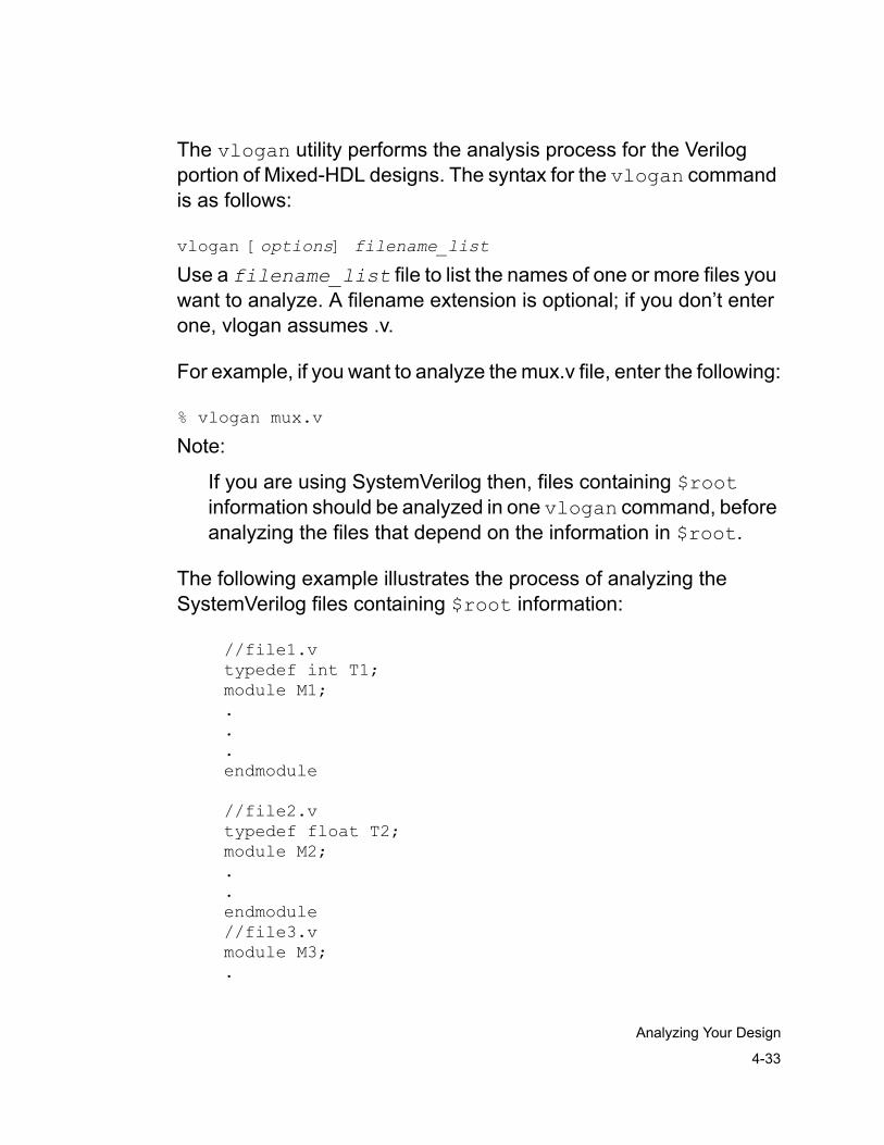
4-33
Analyzing Your Design
The vlogan utility performs the analysis process for the Verilog portion of Mixed-HDL designs. The syntax for the vlogan command is as follows:
vlogan [options] filename_list
Use a filename_list file to list the names of one or more files you want to analyze. A filename extension is optional; if you don’t enter one, vlogan assumes .v.
For example, if you want to analyze the mux.v file, enter the following:
% vlogan mux.v
Note:
If you are using SystemVerilog then, files containing $root information should be analyzed in one vlogan command, before analyzing the files that depend on the information in $root.
The following example illustrates the process of analyzing the SystemVerilog files containing $root information:
//file1.vtypedef int T1;module M1;...endmodule
//file2.vtypedef float T2;module M2;..endmodule//file3.vmodule M3;.
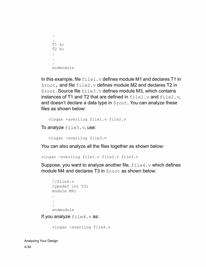
4-34
Analyzing Your Design
.
.T1 a;T2 b;...endmodule
In this example, file file1.v defines module M1 and declares T1 in $root, and file file2.v defines module M2 and declares T2 in $root. Source file file3.v defines module M3, which contains instances of T1 and T2 that are defined in file1.v and file2.v, and doesn’t declare a data type in $root. You can analyze these files as shown below:
vlogan -sverilog file1.v file2.v
To analyze file3.v, use:
vlogan -sverilog file3.v
You can also analyze all the files together as shown below:
vlogan -sverilog file1.v file2.v file3.v
Suppose, you want to analyze another file, file4.v which defines module M4 and declares T3 in $root as shown below:
//file4.vtypedef int T3;module M4;...endmodule
If you analyze file4.v as:
vlogan -sverilog file4.v
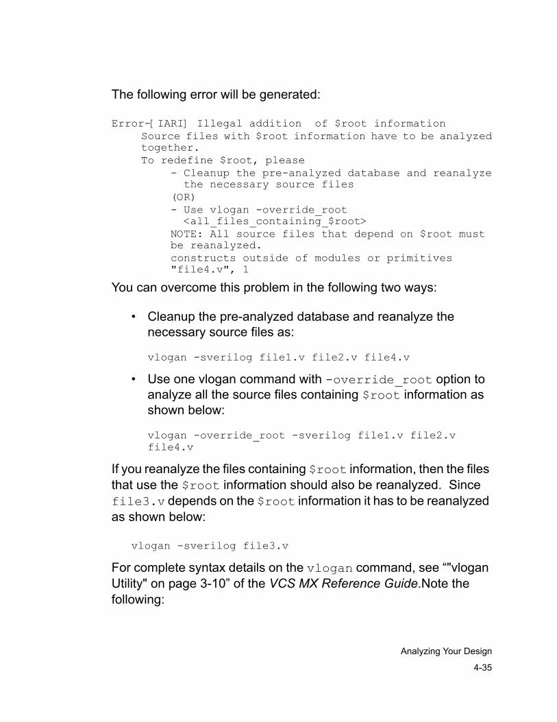
4-35
Analyzing Your Design
The following error will be generated:
Error-[IARI] Illegal addition of $root informationSource files with $root information have to be analyzedtogether.To redefine $root, please
- Cleanup the pre-analyzed database and reanalyzethe necessary source files
(OR)- Use vlogan -override_root<all_files_containing_$root>
NOTE: All source files that depend on $root mustbe reanalyzed.constructs outside of modules or primitives"file4.v", 1
You can overcome this problem in the following two ways:
• Cleanup the pre-analyzed database and reanalyze the necessary source files as:
vlogan -sverilog file1.v file2.v file4.v
• Use one vlogan command with -override_root option to analyze all the source files containing $root information as shown below:
vlogan -override_root -sverilog file1.v file2.v file4.v
If you reanalyze the files containing $root information, then the files that use the $root information should also be reanalyzed. Since file3.v depends on the $root information it has to be reanalyzed as shown below:
vlogan -sverilog file3.v
For complete syntax details on the vlogan command, see “"vlogan Utility" on page 3-10” of the VCS MX Reference Guide.Note the following:
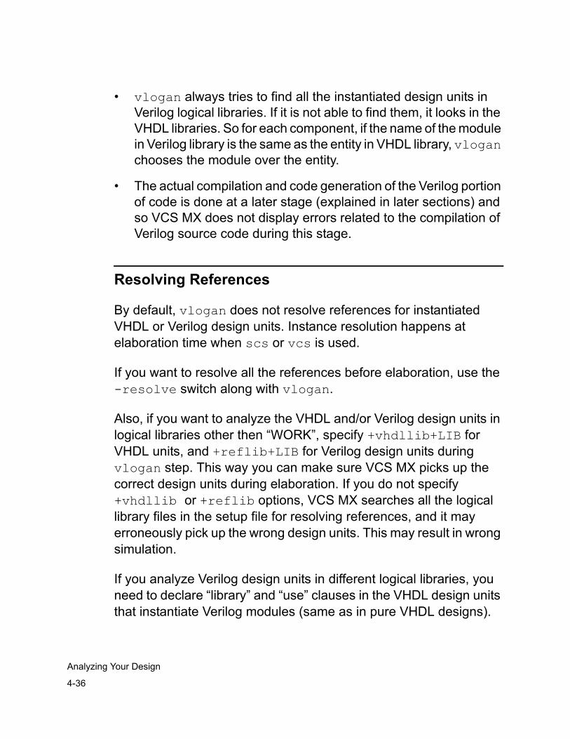
4-36
Analyzing Your Design
• vlogan always tries to find all the instantiated design units in Verilog logical libraries. If it is not able to find them, it looks in the VHDL libraries. So for each component, if the name of the module in Verilog library is the same as the entity in VHDL library, vlogan chooses the module over the entity.
• The actual compilation and code generation of the Verilog portion of code is done at a later stage (explained in later sections) and so VCS MX does not display errors related to the compilation of Verilog source code during this stage.
Resolving References
By default, vlogan does not resolve references for instantiated VHDL or Verilog design units. Instance resolution happens at elaboration time when scs or vcs is used.
If you want to resolve all the references before elaboration, use the -resolve switch along with vlogan.
Also, if you want to analyze the VHDL and/or Verilog design units in logical libraries other then “WORK”, specify +vhdllib+LIB for VHDL units, and +reflib+LIB for Verilog design units during vlogan step. This way you can make sure VCS MX picks up the correct design units during elaboration. If you do not specify +vhdllib or +reflib options, VCS MX searches all the logical library files in the setup file for resolving references, and it may erroneously pick up the wrong design units. This may result in wrong simulation.
If you analyze Verilog design units in different logical libraries, you need to declare “library” and “use” clauses in the VHDL design units that instantiate Verilog modules (same as in pure VHDL designs).
5-1
Compiling Your Design
5Compiling and Elaborating Your Design 4
The VCS MX compiler compiles and elaborates your design. It can be run using two different commands:
• For the VHDL-only and VHDL-top flows, the scs command elaborates your design, generates code,compiles C code, and statically linkins all objects in order to generate executable binary file, called scsim, for running the simulation.
• For Verilog-only and Verilog-top flow, the vcs command generates an executable binary, called simv, for running the simulation.
Note:The word “compilation” is used throughout this chapter to mean elaborate and compile the design.
5-2
Compiling Your Design
This chapter contains the following sections:
• Understanding the VCS MX Compilation Process
• Using the scs Command
• Using the vcs Command
Understanding the VCS MX Compilation Process
The VCS MX compilation process takes place after you’ve analyzed any VHDL or Verilog source in your mixed-HDL design. If your design contains only Verilog code, then this is the first step of the simulation process.
The VCS MX Compiler expands the design hierarchy given a design root, and produces the executable binary file for simulation.
Either of the following executables are used during the compilation step:
• For VHDL-only or VHDL-top designs, use the scs executable. Note that when running VHDL-top, you must also include the -mhdl flag. Note also that you can pass any Verilog compile-time options by specifying the -Verilogcomp option and the appropriate option inside double-quotes.
• For Verilog-only or Verilog-top designs, use the vcs executable. Note that when running Verilog-top, you must also include the -mhdl flag. Note also that you can pass any VHDL compile-time options by specifying the -vhdlelab option and the apppropriate option inside double-quotes.
5-3
Compiling Your Design
Both the scs and vcs executables are discussed in detail throughout this chapter:
• For details on scs, see “Using the scs Command,” in the next seciton.
• For detials on vcs, see the “Using the vcs Command” on page 4-50.
Using the scs Command
This section describes the process for using the scs command for compiling and elaborating your design.
The syntax for the scs command is the following:
scs [options] design_root
For example, to compile the entity CPU with the configuration CPU_cfg, enter the following:
% scs CPU_cfg
To compile the entity MUX using the architecture behavioral, enter the following:
% scs mux behavioral
To compile the entity E, enter the following:
% scs E

5-4
Compiling Your Design
In the example, since no architecture is specified, the most recently analyzed architecture for this entity is used.
For VHDL-top designs, both the VHDL top entity/configuration, as well as dangling Verilog-top modules are supported.
You can specify as many as dangling Verilog top modules at the scs command line as needed. For example:
scs -mhdl cfg -vltop <dangling verilog top> -vltop <dangling verilog top> -verilogcomp " ... "
Common scs Compilation Options
Some of the more commonly used scs options enable the following:
• Compiling for Simulation Mode
• Modifying Cycle Simulation Compilation
• Overriding Generics Values
• Creating Multiple Simulation Executables
• Setting Time Base and Time Resolution
For a complete description of all scs options, see the “scs Command and Options” section in Chapter 4, "Compilation Options" of the VCS MX Reference Guide.
Compiling for Simulation Mode
After analyzing a design with the proper options, the design can be partitioned into event and cycle blocks, compiled, and then the design is ready for simulation.
5-5
Compiling Your Design
VCS MX is highly optimized to deliver the fastest simulation results possible for most designs. To obtain the fastest simulation with VCS MX, use the following guidelines:
• Simulate the entire design and testbench in cycle mode.
• In some cases, it might not be possible to simulate everything in cycle mode. Typically, this is due to a more behavioral style in the testbench which does not meet the cycle style requirements (see the VHDL Simulation Coding and Modeling Style Guide). In this case, the fastest simulation results can be obtained by partitioning the design between event and cycle simulation modes.
In general, you can compile your design to simulate in one of the following simulation modes
• Event-Driven Simulation
• Mixed Event and Cycle-based Simulation
• Full Cycle-based Simulation
Event-Driven Simulation
Typically, you use debug mode and compiled mode event simulation in the early stages of the design when you are making frequent changes to your VHDL source code. Debug mode event simulation provides you full access to your code enabling you to do source-line debugging. Compiled mode event simulation still allows full visibility into the design and offers you better performance than debuggable event mode.
For example to compile the CPU design for event simulation, the command
% scs -nc CPU_TOP
5-6
Compiling Your Design
creates the executable binary file named scsim that you then run to start the simulation. Note that the -nc option is used to suppress printing the copyright banner.
Mixed Event and Cycle-based Simulation
VCS MX combines the flexibility of event-driven simulation with performance of cycle-based simulation. As portions of your design become stable, you can start to run in compiled event or mixed event and cycle mode, increasing the simulation speed of those blocks. Mixed mode simulation provides the maximum performance while compiled event simulation supports the full VHDL language.
To run a mixed mode simulation, you must create a partition file to identify the design subtrees or blocks to run in cycle mode. See the “Creating a Partition File” section in this chapter for information about how to create this file.

5-7
Compiling Your Design
Figure 5-1 Design example
Consider the example design in Figure 5-1. To simulate the design in mixed event and cycle mode, where sub1 and sub2 blocks are partitioned to run in cycle and the rest of the design to run in event, a partition file with the partition information is created (part.file). The top-level of the design, TB_TOP_CFG, is analyzed into the library work. The command to compile the design is
% scs -partition part.file work.tb_top_cfg
TB_TOP_CFG
design_top
sub1 sub2
leaf1 leaf2 leaf3 leaf4
5-8
Compiling Your Design
Multi-Layers of Event and Cycle PartitionsThis is also know as event and cycle “donuts”. By default, all design units are run in event mode. Once a design block is specified to run in cycle, that entire design block simulates in cycle mode. If there is a sub-block of behavioral IP or some non-cycle VHDL code in that design cycle region, you can specify an event partition (event donut) for that design unit in the partition file. Event partitions are similar to cycle partitions in that once a design block is identified to run in event, all design units below that will be in event mode. In general, you can have multiple layers of event and cycle partitions, but the best simulation performance is achieved when the whole testbench and design are running in cycle, or when the design is running in cycle while the testbench is running in event.
Full Cycle-based Simulation
If the entire design and testbench comply with the cycle modeling and coding style guidelines and they are compiled for cycle simulation, the entire simulation can be performed in cycle mode.
Due to the high levels of optimizations performed for cycle simulation, use this mode only with relatively stable designs as the debugging capabilities are limited compared to debug event mode.
For a full cycle simulation, a partition file with a single cycle statement is required to enable full cycle simulation. The top level configuration for the simulation is identified in the partition file’s cycle statement (this is the same configuration identified on the scs command line). See the “Creating a Partition File” section in this chapter for more information on how to create the partition file.
5-9
Compiling Your Design
Creating a Partition File
The partition file contains all the necessary information to divide a design into event and cycle blocks. A partition file must be created to perform mixed event and cycle simulation or full cycle-based simulation.
When creating a partition file, consider the following guidelines:
1. For each design block that is to run in cycle mode, you must specify a partition statement in the partition file for the block’s root design unit, otherwise the entire block runs in event mode.
2. If an error is detected in the partition file, scs quits with an error.
3. To add a comment to the partition file, begin the line with # character.
4. Line continuation is not allowed.
5. The partition file is case sensitive and all options must be specified in lower case. The names of the specified library and design unit are not case sensitive, following VHDL semantics.
6. If the root design unit of a cycle block is specified in the partition file multiple times, the options of the last occurrence of the root design unit in the partition file are the one used.
7. In your partition file, you can specify your event or cycle block(s) as an entity or a configuration. If you have declared a VHDL configuration for the root design unit of the cycle block and want to use it when instantiating the block, you must include a "use configuration" clause in the VHDL configuration of the design unit that instantiates the partitioned design unit. Be sure to analyze the configuration VHDL source (and all source that comprises the cycle block) so that they run in the correct simulation mode.
5-10
Compiling Your Design
With a VHDL configuration declared and "use configuration" clause in place, VCS MX uses this configuration regardless of whether you specify an entity or a configuration for the root design unit of the cycle block in the partition file.
8. If the configuration name of the root of the cycle block is specified in the partition statement and no use clause is found for that configuration in the VHDL, VCS MX issues an error and quits.
9. If you have not declared a configuration for the root design unit of the cycle block, you must specify the entity for that root design unit in the partition file. If you specify a configuration that is not declared, VCS MX issues an error and quits.
10. If you have multiple architectures for the root design unit of the cycle block, a configuration must be specified in the partition file to allow the determination of the correct architecture (along with specifying the “use configuration” clause in the VHDL source).
11. If an entity/arch pair is specified in the partition file, an error occurs.
5-11
Compiling Your Design
Partition Statement SyntaxCycle Partitioncycle [-2state | -4state] [-perf | -noperf]
[-latch_transparency] [-latch_style style] [-tbl] [libname.]design_unit
Event Partitionevent [libname.]design_unit
Options
-2state
Creates 2-state (0,1) executable code. 2-state code allows Z values for bus signals. 2-state code is faster than 4-state code. The -2state option and the -4state option are mutually exclusive.
-4state
Creates 4-state (0, 1, X, Z) code. The -4state option and the -2state option are mutually exclusive. 4-state code is the default code generated.
-perf
Creates a version of executable code that is fully optimized and less observable (limited debugging). This option is on by default. Code generated using -perf is faster than code generated with -noperf. The -perf and -noperf options are mutually exclusive.
-noperf
Creates a version of executable code that is more observable than with the -perf. Simulating the cycle portion of your design in debug mode is equivalent to specifying every signal and variable in the cycle block as read mode in a monsigs file. The -noperf option and the -perf option are mutually exclusive.
5-12
Compiling Your Design
-latch_transparency
Makes all latch based processes use their sensitivity list as the trigger instead of the enable. This is a dangerous option, use it only in flip-flop based designs containing few latches. This option causes a significant performance degradation.
-latch_style style
Specifies the type of edge to be used as the trigger edge. The possible choices for style are leading, trailing, or event (which triggers on both the leading and trailing edge).
-tbl
Enables VCS MX table optimization for the cycle portions of the design. To enable table optimization and specify how you want VCS MX to evaluate the tables, you can use the cycle command-line options listed in Table 5-1.
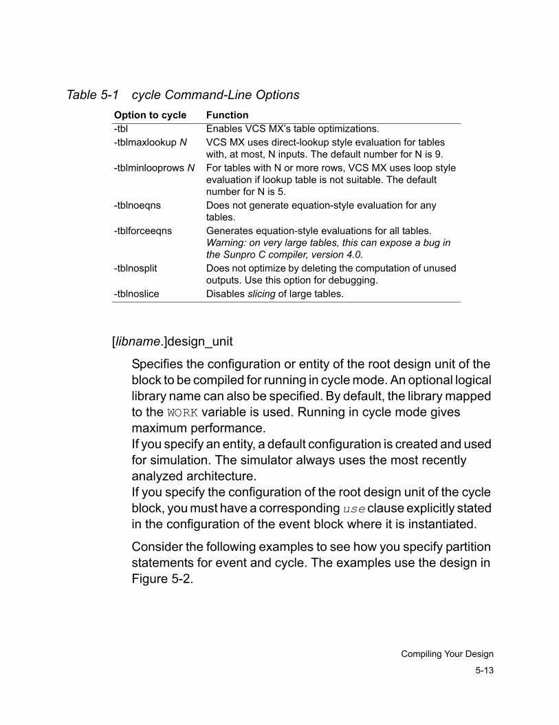
5-13
Compiling Your Design
Table 5-1 cycle Command-Line Options
[libname.]design_unit
Specifies the configuration or entity of the root design unit of the block to be compiled for running in cycle mode. An optional logical library name can also be specified. By default, the library mapped to the WORK variable is used. Running in cycle mode gives maximum performance.If you specify an entity, a default configuration is created and used for simulation. The simulator always uses the most recently analyzed architecture.If you specify the configuration of the root design unit of the cycle block, you must have a corresponding use clause explicitly stated in the configuration of the event block where it is instantiated.
Consider the following examples to see how you specify partition statements for event and cycle. The examples use the design in Figure 5-2.
Option to cycle Function-tbl Enables VCS MX’s table optimizations.-tblmaxlookup N VCS MX uses direct-lookup style evaluation for tables
with, at most, N inputs. The default number for N is 9.-tblminlooprows N For tables with N or more rows, VCS MX uses loop style
evaluation if lookup table is not suitable. The default number for N is 5.
-tblnoeqns Does not generate equation-style evaluation for any tables.
-tblforceeqns Generates equation-style evaluations for all tables. Warning: on very large tables, this can expose a bug in the Sunpro C compiler, version 4.0.
-tblnosplit Does not optimize by deleting the computation of unused outputs. Use this option for debugging.
-tblnoslice Disables slicing of large tables.
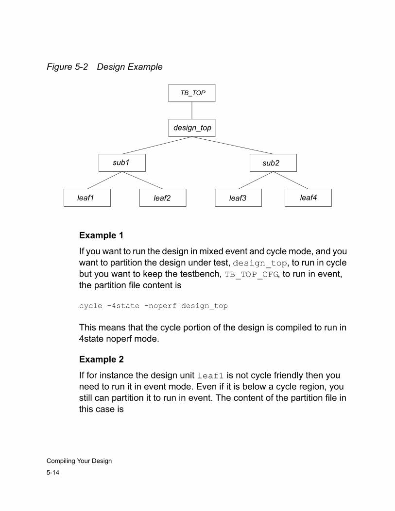
5-14
Compiling Your Design
Figure 5-2 Design Example
Example 1
If you want to run the design in mixed event and cycle mode, and you want to partition the design under test, design_top, to run in cycle but you want to keep the testbench, TB_TOP_CFG, to run in event, the partition file content is
cycle -4state -noperf design_top
This means that the cycle portion of the design is compiled to run in 4state noperf mode.
Example 2
If for instance the design unit leaf1 is not cycle friendly then you need to run it in event mode. Even if it is below a cycle region, you still can partition it to run in event. The content of the partition file in this case is
TB_TOP
design_top
sub1 sub2
leaf1 leaf2 leaf3 leaf4
5-15
Compiling Your Design
cycle -4state -noperf design_top_cfgevent leaf1
Note that the partition statement uses the configuration name of the design under test, design_top_cfg. In this case, the TB_TOP_CFG configuration must specify to use the configuration of design_top explicitly.
configuration TB_TOP_CFG of TB_TOP is for A for DUT : design_top
-- Explicit use clause to specify the cycle -- configuration use configuration WORK.design_top_cfg; end for; end for;end TB_TOP_CFG;
Example 3
If a partition file has multiple partition statements that apply to the same configuration, the bottom line overrides the previous one.
cycle -2state -noperf design_top_cfgcycle design_top_cfg
The cycle block is compiled in 4state perf mode (the default), and not in 2state noperf mode.
Example 4
Consider the partition below
5-16
Compiling Your Design
event sub2cycle -latch_style leading sub1
Again, multiple partitions are specified. The first partition compiles the entity sub2 in event. This partition is not necessary unless the design region above design_root is being simulated in cycle mode. The second partition compiles the design block under sub1 in cycle. The -latch_style option is used to tell VCS MX compiler to create a trigger on the positive edge of any latches instead of on the default negative edge.
Example 5
Consider the partition below
cycle design_topevent sub2cycle leaf4
Multiple partitions are specified. The first partition specifies to compile the design top-level design_top in cycle. The second partition specifies to compile the design sub-block sub2, which is under design_top, in event (an event donut). The final partition specifies to compile the entity leaf4 in cycle.
Modifying Cycle Simulation Compilation
When you compile your design for mixed event and cycle mode or full cycle-based mode, you can use scs command line modifiers to
• Compile for 2-state simulation
• Compile for performance or debugging
• Select a compiler
5-17
Compiling Your Design
• Pass options to the compiler
• Generating static elaboration reports
Compiling for 2-State Simulation
The -2state option tells the compiler to create code that simulates in <0,1> (2-state) mode for the cycle blocks. 2-state code is faster than 4-state code.
You cannot use the 2-state mode if the VHDL code contains explicit ‘X’s. This produces an error. You must then use the default, <0,1,X> (4-state) mode. The 4-state mode allows unknown values to be propagated through logic gates.
The Z state is available in both modes. In cycle simulation, Z is treated as a metavalue associated with the outputs of 3-state devices and buses (resolved bidirectional ports and the nets associated with them).
For example,
% scs -2state -partition part.file design_cfg
Note:Using the -2state option on the scs command line will change the default code generation to 2-state for all cycle design partitions. Explicitly using the -4state option in the partition file overrides this setting.
5-18
Compiling Your Design
Compiling for Performance or Debugging
One of the ways cycle simulation improves performance is by optimizing away internal variables and signals. VCS MX Compiler can generate code at two different levels of optimization for cycle mode, providing a trade-off of runtime performance against ease of debugging. In the fully optimized -perf (performance) mode, observability is limited to ports and states (registers). In -noperf (debug) mode, all objects in the cycle blocks are observable.
To achieve maximum performance, the default optimization level is the performance mode. You can override this setting by specifying the -noperf on the scs command line, or in the partition file for each cycle block.
Creating a Monsigs FileUsing the -noperf option makes all objects in the cycle blocks observable, but it slows the simulation down. But if you are interested only in few internal objects and you do not want to compromise the overall performance, you can use the -monsigs option to keep only those objects visible and still run in performance mode.
Moreover, using the -monsigs option allows you to specify whether you want to trace and/or assign (write) values to the specified signals and variables in the monsigs file.
You specify the -monsigs option on the scs command line along with the -partition option, for example,
% scs -perf -monsigs mon.file -partition part.file design_cfg
When creating a monsigs file, consider the following guidelines:
5-19
Compiling Your Design
1. To add a comment to the monsigs file, begin the line with # character.
2. Line continuation is not allowed.
3. Wildcarding is not allowed.
4. The monsigs file is not case sensitive.
5. Any additional white space is ignored.
Syntax[r] [t] [w] : /top_level_design_entity/full_name
Statement Optionsr
Keeps the specified signal or variable values visible for reading and unoptimized tracing. If you plan to trace some specific signals or variables, use the t option of monsigs for those objects. Using the r option on all signals and variables in a cycle block of your design is equivalent to using the -noperf option for partitioning the block.
t
Keeps the specified signal or variable values visible for reading and optimized tracing. Using this option to specify signals or variables to be traced within a cycle region, yields faster simulation performance than if they are specified with the r option or the -noperf option for partitioning the block. See the See “dump” on page 6-62 of the VCS MX Reference Guide for information about how to automatically generate a monsigs file.
5-20
Compiling Your Design
w
Keeps the specified signal or variable values visible for reading, unoptimized tracing, and writing. This option lets you assign and hold values in a cycle region. Specifying w is equivalent to specifying r and w. Note that this option slows the simulation performance. Do not use it on a large number of signals. The -noperf option does not provide write permissions for signals and variables.
top_level_design_entity
Specifies the name of the top-level entity of the design.
full_name
Specifies the full name of the VHDL signal or variable you want to remain visible. The full pathname to the object from the top-level design entity must be specified. If only a path is specified, all signals and variables in the specified design region remain visible.
Examples# keep Data_bus readable and traceabler t : /TB/DUT/U0/Data_bus
# keep Addr_bus readable, writable, and traceablew t : /TB/DUT/U0/Addr_bus
# keep reset_sig readable and writablew : /TB/DUT/reset_sig
# keep all objects in U1 instance readable and traceablet : /TB/DUT/U1
5-21
Compiling Your Design
Selecting a C Compiler
The default compiler used by VCS MX Compiler is defined by the platform-specific CS_CCPATH_$ARCH setup variable. To select a different compiler, use the -ccpath "compiler" modifier, for example,
% scs -ccpath “compiler” -partition part.file design_cfg
Note:It is recommended that you use the same C compiler for both event and cycle C compilation. Otherwise, problems may occur during static linking of the simulation executable binary file.
Passing Options to the C Compiler
Use the -ccflags "option_string" to pass options to the C compiler. For example, some compilers have trouble compiling large files when the compiler optimize option is on. To lower the optimization level, replace the -O option with -O1 in the default option string. By default, VCS MX Compiler passes the options specified by the CS_CCFLAGS_$ARCH setup variable.
For example, on a Sun SPARCOS5 platform, to speed up compilation by decreasing the C compiler optimization settings, enter
% scs -ccflags ”-c -O1” -partition part.file design_cfg
Synopsys provides the gcc C compiler for use with the Sun SPARCOS5 platform. The C compiler flags are already set for optimized code generation and we do not recommend that you change them.
Table 5-2 shows the optimize option for each platform.

5-22
Compiling Your Design
Table 5-2 Platform-Specific Flags for scs -ccflags
Generating Static Elaboration Reports
You can generate static elaboration report for the cycle block by using the following option on your scs command line
% scs -perf_data report.txt -partition part.file design_cfg
This report shows detailed information about the optimizations made to the cycle design block during compilation. See the “Static Cycle Elaboration Reports” section for more information about how to read the report.
Overriding Generics Values
A generic can be declared anywhere in the design hierarchy. The following list shows how you can assign a value to a generic in your design. It is listed in order of precedence for conflicting assignments:
1. From a command file
2. In the VHDL source code
Platform -ccflags “option_string” Optimize Option
sparcOS5 “-c -O” -O
hpux10 “-c -w -O -Ae” -O
linux “-c -O” -O
rs6000 “-c -qchars=signed -O -qmaxmem=2048000”
-O
5-23
Compiling Your Design
An assignment to a generic value from a command file overrides the assignment from the value defined in the VHDL source code. These generic assignments must be know by compilation time in order to correctly determine any variable object sized determined by generic values.
Changing the Generic Parameter Default Value
You can change the default value of a generic by modifying the design’s VHDL source file. To apply this value, you must reanalyze the source file. The next method avoids the necessity of reanalyzing the file.
Assigning Generic Values from a Command File
After analyzing your design, you can override the default value for any generic by using a command file specified on the scs command line, as follows:
% scs -generics cmdfile design_cfg
cmdfile is an include file that contains only simulator assign commands targeting design generics. The absolute hierarchical path for the generic whose value is to be reassigned must be provided in the generics file.
Before compiling the design, scs reads, displays, and applies the assignments in cmdfile.
Example 1
If you have a top-level generic in the entity TB to define a clock period declared as
5-24
Compiling Your Design
generic (PERIOD : time := 1000 ns);
We can double the clock speed by cutting the period in half to 500 ns. The command file to assign the new value to PERIOD looks like
assign (500 ns) /TB/PERIOD
Note:Note the usage of parenthesis for physical units.
To invoke scs using this command file, type
% scs -generics generics.input design_cfg
generics.input is the command file containing the assign statement.
The resulting output from scs is
GENERIC ASSIGNMENTS FROM FILE "generics_file":assign (500 ns) /TB/PERIOD
The value of PERIOD is changed to 500 ns.
For top-level generics, generics declared at the top-level in the design hierarchy, the absolute hierarchical path to the generic is not needed although providing the absolute path is still recommended. For the example above, we could have specified simply the generic name like
assign (500 ns) PERIOD
and still have correct results. If PERIOD is not declared in the top-level design unit, an elaboration error would occur.
5-25
Compiling Your Design
Example 2
You can assign same value to multiple generic targets with one assign command in the generics file.
assign ‘0’ /TB/TOP/U1/STOP_FLAG /TB/TOP/U2/READY_FLAG
Note that in mixed langauge simulation, the above command needs to be specified differently to accomodate the mixed language environment.
assign {“0”} /TB/TOP/U1/STOP_FLAG /TB/TOP/U2/READY_FLAG
Example 3
You can assign same value to multiple generic targets (with same name) with one assign commands in the generics file without having to specify the path for each of them.
assign (20 ns) tpdassign (10 ns) /top/u1/tpd
Here all tpd generics will have 20 ns with the exception of /top/u1/tpd which will have 10 ns since second more specific assign command will overwrite the more general first assign command.
The order of assign commands is important!
assign FALSE TimingChecksOnassign TRUE u2/TimingChecksOn
Here all TimingCheckOn will be FALSE with the exception of all TimingChecksOn under all components named u2 which are TRUE.
Note that with the above example, you can now control turning on/off timing checks for VITAL components selectively or for all
5-26
Compiling Your Design
components. This is another way to turn timing checks off in addition to the already supported way via the variables in the synopsys_sim.setup file.
LimitationYou cannot use the above method to override the default values for lower level Verilog parameters.
Example 4You can assign a value from a Verilog instance to a generic using a VHDL path in a command file. For the hierarchy:
e (VHDL) -->uut (VHDL) -->convert (VHDL instance of Verilog implementation) -->z_1 (Verilog instance at VHDL implementation for z_1)
You can specify the value of generic g1 as shown below. Note that the VHDL portion of the hierarchy is case insensitive, while the Verilog portion (module, instances) is case sensitive.
assign 1 /e/uut/convert/z_1/G1(valid)assign 1 /e/uut/convert/z_1/g1(valid)assign 1 /E/Uut/Convert/z_1/g1(valid)assign 1 /e/uut/convert/Z_1/g1(Invalid because Verilog instance z_1 is case
sensitive.)
Creating Multiple Simulation Executables
You can use the -executable option to name the generated simulation executable binary. Default name for the simulation executable is scsim.
5-27
Compiling Your Design
For example, to name the simulation executable mysim instead of the default scsim, type
% scs -executable mysim design_cfg
By default, each generated executable has an associated database directory (by default scsim.db.dir) that is used to store all necessary information for that executable to run simulation. The simulator has no dependencies on any of the VHDL work libraries that the design VHDL files are analyzed to. This enables you to
• Create multiple executables where each is compiled with different scs options. For example, one for debug simulation, another for compiled event simulation, and a third for cycle simulation.
• Relocate running the simulation to another directory as long as you move both the executable and its database directory together, and also any other input files needed for running the simulation.
Note:If you want to rename a simulation executable after it is created, you must ensure to rename both the simulation executable and its database directory.
Setting Time Base and Time Resolution
You can use the -time option to set the time base for the simulation. This option overrides the default TIMEBASE variable value in the setup file. -time option takes argument, base_time, valid values for base_time are as follows:
• fs femtoseconds
• ps picoseconds
5-28
Compiling Your Design
• ns nanoseconds
• us microseconds
• ms milliseconds
• sec seconds
The default value for base_time is ns.
For example, to set the simulation time base to ps instead of the default ns, type
% scs -time ps design_cfg
In addition to setting the time base, you can also specify the simulator time resolution with the -time_resolution option. Setting the time resolution basically sets the precision or the number of simulation ticks per base time unit. The format for using -time_resolution is as follows:
-time_res[olution] [1 | 10 | 100] [fs | ps | ns | us | ms | sec]
If a value beside 1, 10, or 100 is provided, a warning during scs will be issued and a default setting of 1 <unit> will be used (where unit is the specified time unit (fs, ps, etc.)).
Note:Time resolution value cannot be higher than the time base value. An error will be issued if this happens.
If no numeric value (1, 10, or 100) is provided, then the default value is 1. For example:
% scs -nc -time_res ps design_cfg
5-29
Compiling Your Design
To set the simulation time resolution to 10ps instead of the default 1ns, type
% scs -nc -time ns -time_res 10ps design_cfg
The -time_resolution option to the scs command overrides the TIME_RESOLUTION value in the setup file.
Using Time Resolution
When you specify a time resolution for a simulation, pay attention to its effect on the values of time objects and delays in the VHDL source, the simulation user interface (UI), Mixed HDL simulation, and VHPI.
wait for or after statements in the VHDL SourceIf the VHDL source contains time delays (using wait for or after statements) that are smaller than the time resolution value, then the delays will be rounded up or down to the next closest unit specified for the time resolution. If time resolution is not set, then time delays will be compared with time base value.
For example, if the resolution is set to 1 ns, and in the VHDL source contains:
wait for 1.4 ns;
The delay will be rounded down to 1 ns (equivalent to wait for 1 ns;). And if the VHDL source contains:
wait for 1.5 ns;
The delay will be rounded up to 2 ns (equivalent to wait for 2 ns;)
5-30
Compiling Your Design
Assertion statementsTime in VHDL assertions will be printed in units of the time resolution.
VCS MX User Interface (TCL/UI)Values of type time are displayed in VCS MX UI in terms of time resolution units. This includes displaying the $now simulator variable.
Note:Displaying $now simulator variable in the UI is changed. The value is now displayed as a value with a time unit. For example,
# echo $now100 PS
This is different from previous VCS MX releases. If you have TCL scripts or procedures that operate/use $now, you may want to make note of this. If you want to keep the old way of displaying $now, then you need to set off a variable so you can keep the backward compatibility. The TCL variable name is display_now_unit. For backward compatibility, type at the simulation prompt
# set display_now_unit FALSE
Any specified time unit in the TCL UI that is given without a timebase (fs, ns, etc) will use units of TIMEBASE. Examples (with TIMEBASE = NS and TIME_RESOLUTION = 10 PS)
# run 1
Will run for 1 NS (advances the simulation by 1000 PS).
# run 1.1 ns

5-31
Compiling Your Design
Will run for 1.1 NS (advances the simulation by 1100 PS).
# run 5 ps
Will truncates the time to 0 PS and advances the simulation by 0 PS.
# run 102 ps
Will truncates the time to 100 PS and advances the simulation by 100 PS.
# run 1.005 ns
Will truncate the time to 1.000 NS (advances the simulation by 1000 PS).
Mixed HDL SimulationFor Mixed HDL, the simulator precision is set to the highest resolution needed in either the VHDL or the Verilog. The definition for time unit and precision for each language is the following:
• For Verilog
`timescale unit/precision
`timescale 1ns/10ps - 1ns is the unit, 10ps is the precision
• For VHDL:
TIME_RESOLUTION = precision
TIMEBASE = unit
TIME_RESOLUTION = 10ps - this is the time precision
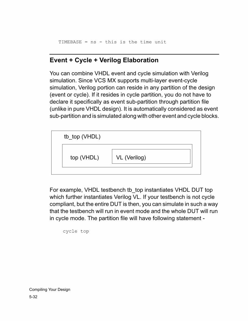
5-32
Compiling Your Design
TIMEBASE = ns - this is the time unit
Event + Cycle + Verilog Elaboration
You can combine VHDL event and cycle simulation with Verilog simulation. Since VCS MX supports multi-layer event-cycle simulation, Verilog portion can reside in any partition of the design (event or cycle). If it resides in cycle partition, you do not have to declare it specifically as event sub-partition through partition file (unlike in pure VHDL design). It is automatically considered as event sub-partition and is simulated along with other event and cycle blocks.
For example, VHDL testbench tb_top instantiates VHDL DUT top which further instantiates Verilog VL. If your testbench is not cycle compliant, but the entire DUT is then, you can simulate in such a way that the testbench will run in event mode and the whole DUT will run in cycle mode. The partition file will have following statement -
cycle top
tb_top (VHDL)
top (VHDL) VL (Verilog)
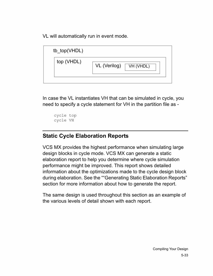
5-33
Compiling Your Design
VL will automatically run in event mode.
In case the VL instantiates VH that can be simulated in cycle, you need to specify a cycle statement for VH in the partition file as -
cycle topcycle VH
Static Cycle Elaboration Reports
VCS MX provides the highest performance when simulating large design blocks in cycle mode. VCS MX can generate a static elaboration report to help you determine where cycle simulation performance might be improved. This report shows detailed information about the optimizations made to the cycle design block during elaboration. See the ““Generating Static Elaboration Reports” section for more information about how to generate the report.
The same design is used throughout this section as an example of the various levels of detail shown with each report.
top (VHDL)VH (VHDL)VL (Verilog)
tb_top(VHDL)
5-34
Compiling Your Design
Reading Summary Information
The most basic data in the cycle static elaboration report is a summary that contains basic optimization information for the cycle design unit. The summary shows basic details on various aspects of the cycle design unit.
The following information are shown in the summary:
• Number of combinational signals
The number of combinational signals in the cycle design unit. A combinational signal does not have a latched value.
• Number of sequential signals
The number of sequential signals in the cycle design unit. A sequential signal has a value that is being latched in the design.
• Number of bus signals
The number of bused signals in the cycle design unit. A bused signal is a signal that has multiple drivers for it.
• Number of seq processes (post-split)
The number of processes in the cycle design unit with state information. This number is calculated after various optimizations are done to split synchronous and asynchronous design regions.
• Number of combinational processes
The number of processes in the cycle design unit that do not contain state information.
5-35
Compiling Your Design
• Number of testbench processes
The number of processes in the cycle design unit that cannot be optimized or must execute at a specific point in time, usually do to a ‘wait for time’ statement. Cycle optimizations are not applied to these processes.
• Number of concurrent assignments
The number of concurrent signal assignments in the cycle design unit.
• Number of testbench functions (tbf)
The number of testbench functions (tbf) created by VCS MX for the cycle design unit. A testbench function is created for simulating any testbench processes. Fewer numbers of testbench functions results in better simulation performance.
• Number of triggers (tgf)
The number of trigger functions (tgf) created by VCS MX. Tgfs are used to execute the sequential processes in the cycle design unit. Multiple sequential processes can be executed by a common tgf. The ratio of the number of tgfs to the number of sequential processes is a good indication of the amount of cycle optimizations occurring. Fewer trigger functions controlling large numbers of sequential processes result in better simulation performance.
5-36
Compiling Your Design
• Number of combinational functions (cbf)
The number of combinational logic functions (cbf) created by VCS MX. Cbfs are optimized functions containing all the combinational processes and concurrent assignments in the cycle design unit. The ratio of the number cbfs to the number of combinational processes is a good indication of the amount of cycle optimizations occurring. Fewer combinational functions controlling large numbers of combinational processes result in better simulation performance.
• Maximum combinational level depth
The maximum depth of the combinational functions. VCS MX flattens and levelizes combinational logic to improve simulation performance. Because levelization occurs, delta cycles are not needed for cycle simulation. The lower the number of combinational levels, the faster the simulation speed.
• Number of feedback loops
The number of combinatorial feedback loops detected inside the cycle design unit. Combinatorial feedback loops are broken by the simulator to perform cycle optimizations and negatively affect simulation performance.
• Size of data memory
The amount of memory needed (in kilobytes) to store the data for simulating the cycle design unit.
• Size of code memory
The amount of memory needed (in kilobytes) to store the executable code needed to simulate the cycle design unit.

5-37
Compiling Your Design
Adding the data memory and code memory sizes gives a good approximation of the system memory needed to simulation the cycle design unit.
An example of the elaboration summary data is shown in Example 5-1. The design unit TOP__SCHEMATIC is small, requiring only 32.3 Kb of memory to simulate. This design unit contains 15 sequential and 26 combinational signals, 9 sequential processes, 8 combinatorial processes, and 12 concurrent assignment statements. Based on the coding style, VCS MX was able to optimize this into 3 trigger functions (tgfs) and 20 combinatorial functions (cbfs).
Example 5-1 Static Elaboration Summary Output
CYCLE ELABORATION SUMMARY OF 'TOP__SCHEMATIC' ------------------------------------------------ ================== Elaboration Summary ===============
Number of combinational signals = 26 Number of sequential signals = 15 Number of bus signals = 0 Number of seq processes (post-split) = 9 Number of combinational processes = 8 Number of testbench processes = 0 Number of concurrent assignments = 12 Number of testbench functions (tbf) = 0 Number of triggers (tgf) = 3 Number of combinational functions (cbf) = 20 Maximum combinational level depth = 2 Number of feedback loops = 0
Size of data memory = 1.05 KB Size of code memory = 30.08 KB
===== End of CYCLE ELABORATION Summary for this Design ======
5-38
Compiling Your Design
Reading Triggers Information
Following the summary in the cycle static elaboration report is a table containing detailed information describing each trigger function (tgf). Optimizing tgfs is typically the best way to improve simulation performance of a cycle design unit. Summary Information for each trigger is presented in columns in the elaboration report, listing the following information:
No.
The number associated with the trigger. Triggers are listed in order by the cause of the trigger and how much code they control. Triggers that are expensive to execute are typically listed first, followed by triggers that control large numbers of sequential processes. When trying to improve simulation performance, these triggers must be investigated first.
id
The identification number associated with the tgf. This identification number can be used in conjunction with the -perf_data report to find out which VHDL processes are being controlled by the tgf.
SeqPr
The number of sequential processes being controlled by the tgf. The ratio of the number of tgfs to the number of sequential processes is a good indication of the amount of cycle optimizations occurring. Fewer trigger functions controlling large numbers of sequential processes result in better simulation performance.
Cbf
The number of combinatorial functions (cbfs) that are driven by the tgf.
5-39
Compiling Your Design
CombPr
The number of combinational processes driven by the trigger function. These combinational processes are optimized into the listed cbfs. If a large percentage of the combinatorial processes are driven by a single trigger, improving the performance of the tgf has a greater impact on the overall simulation performance because it is driving most of the design block.
Lev
The maximum levels of the cbfs. A value of -1 means that no cbfs are being driven by the trigger function.
why
The cause of the trigger function. The following are the four different types of triggers:
normal triggersNormal triggers are ones that are recognized by VCS MX cycle templates and are fully optimized. A typical normal trigger usually consists of a clock and a reset signal.
sensitivity triggerSensitivity triggers are ones that use the sensitivity list of a process as the trigger for the process. Sensitivity triggers usually occur when the process is too complex to infer a normal trigger for. This reduces the number of sequential processes that can be merged into a single trigger reducing simulation performance.
5-40
Compiling Your Design
latch triggerLatch triggers are a special kind of sensitivity trigger created when VCS MX infers latches in the VHDL source that are not recognized as one of the VCS MX cycle latch templates. These typically result from a signal that is not fully assigned in a conditional statement (such as a case or an if statement). See the VHDL Simulation Coding and Modeling Style Guide for more information on recognized latch templates.
loop triggersLoop triggers are created by the existence of combinational feedback loops detected in the VHDL code. These triggers are very expensive and must be removed if possible.
Examples of each of these types of triggers is shown in the ““Examples of Various Trigger Types” section.
trigger_conditions
The conditions on which the trigger function is executed. The following notation is used:
pe(signal)pe means simulation of the tgf is executed on the positive or rising edge of the specified signal.
ne(signal)ne means the simulation of the tgf is executed on the negative or falling edge of the specified signal.
~0(signal)~0 specifies the execution of the tgf when the specified signal is not 0. This usually occurs for asynchronous active-low reset signals or latched signals.
5-41
Compiling Your Design
~1(signal)~1 specifies the execution of the tgf when the specified signal is not 1. This usually occurs for asynchronous active-high reset signals or latched signals.
A typical trigger condition consists of a combination of these conditions. For example, a common trigger condition is
~0(reset) pe(clk)
meaning the specified tgf fires when the reset signal is not equal to zero and there is a rising edge on the clock signal.
The list of triggers is various statistical information helps you determine the level of simulation performance to expect from your design.
An example of the triggers data is shown in Example 5-2. This information is from the same design as the summary information. Since all the triggers are normal triggers activated by a simple clock and reset signals, we can expect good simulation performance from this design.
Example 5-2 Static Elaboration Triggers Output
===================== Trigger Summary ==================
SeqPr = sequential processes the trigger controlsCbf = combinational functions (cbf) the trigger drivesCombPr = total number of combinational processes in CbfsLev = maximum levels of the Cbfs (-1 means no cbfs)loop = trigger due to combinational feedback loopsensi = trigger due to sensitivity list normal = regular trigger
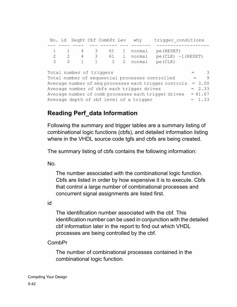
5-42
Compiling Your Design
No. id SeqPr Cbf CombPr Lev why trigger_conditions --- ---- ---- --- ------ --- ------- ------------------- 1 1 4 3 61 1 normal pe(RESET) 2 2 4 3 61 1 normal pe(CLK) ~1(RESET) 3 0 1 1 3 2 normal pe(CLK)
Total number of triggers = 3Total number of sequential processes controlled = 9Average number of seq processes each trigger controls = 3.00Average number of cbfs each trigger drives = 2.33Average number of comb processes each trigger drives = 41.67Average depth of cbf level of a trigger = 1.33
Reading Perf_data Information
Following the summary and trigger tables are a summary listing of combinational logic functions (cbfs), and detailed information listing where in the VHDL source code tgfs and cbfs are being created.
The summary listing of cbfs contains the following information:
No.
The number associated with the combinational logic function. Cbfs are listed in order by how expensive it is to execute. Cbfs that control a large number of combinational processes and concurrent signal assignments are listed first.
id
The identification number associated with the cbf. This identification number can be used in conjunction with the detailed cbf information later in the report to find out which VHDL processes are being controlled by the cbf.
CombPr
The number of combinational processes contained in the combinational logic function.
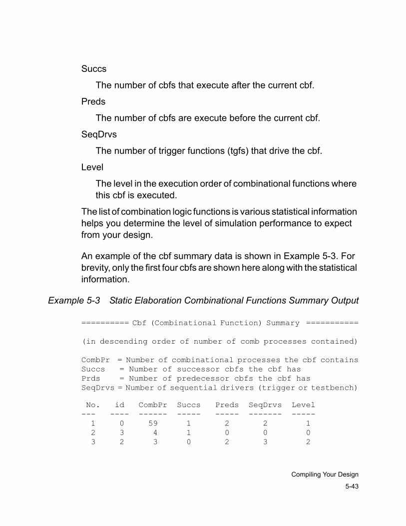
5-43
Compiling Your Design
Succs
The number of cbfs that execute after the current cbf.
Preds
The number of cbfs are execute before the current cbf.
SeqDrvs
The number of trigger functions (tgfs) that drive the cbf.
Level
The level in the execution order of combinational functions where this cbf is executed.
The list of combination logic functions is various statistical information helps you determine the level of simulation performance to expect from your design.
An example of the cbf summary data is shown in Example 5-3. For brevity, only the first four cbfs are shown here along with the statistical information.
Example 5-3 Static Elaboration Combinational Functions Summary Output
========== Cbf (Combinational Function) Summary ===========
(in descending order of number of comb processes contained)
CombPr = Number of combinational processes the cbf containsSuccs = Number of successor cbfs the cbf hasPrds = Number of predecessor cbfs the cbf hasSeqDrvs = Number of sequential drivers (trigger or testbench)
No. id CombPr Succs Preds SeqDrvs Level--- ---- ------ ----- ----- ------- ----- 1 0 59 1 2 2 1 2 3 4 1 0 0 0 3 2 3 0 2 3 2

5-44
Compiling Your Design
4 9 3 0 0 0 0...Total number of combinational functions (cbfs) = 20Total number of combinational processes contained = 97Average number of comb processes each cbf contains = 4.85Average number of successors each cbf drives = 0.50
After the cbf summary listing, detailed information is provided on all the tgfs, cbfs, and testbench functions (tbfs) in the design. This lists all the tgfs, cbfs, and tbfs in the design block and shows detailed information on the VHDL processes contained within each function, and in what source file and line the process occurs.
An example for a tgf is shown in Example 5-4. The Tgf_id is the same id listed in the triggers summary report, and the trigger conditions are relisted. The sequential processes controlled by the tgf are listed, including the full path from the top-level cycle entity where the design unit was partitioned. In this example, the process TIME_INC is controlled by this tgf and is located in the file alarm_counter.vhd on line 21.
Example 5-4 Static Elaboration Detailed Tgf Information
Tgf_id = 2: conditions [ pe(CLK) ~1(RESET) ] {1 event(s)}
Tgf_name [ TOP__SCHEMATIC_0_tgf_2 ]
Controls 4 sequential process(es):
/TOP/T_BLOCK/TSM/SYNCH$Seq[5] [time_state_machine.vhd:64]
/TOP/A_BLOCK/ASM/SYNCH$Seq[11] [alarm_state_machine.vhd:58]
/TOP/A_BLOCK/ACOUNT/TIME_INC$Seq[8] [alarm_counter.vhd:21]
/TOP/T_BLOCK/TCOUNT/_P0$Seq[2] [time_counter.vhd:23]
Triggers total of 3 Cbf(s):
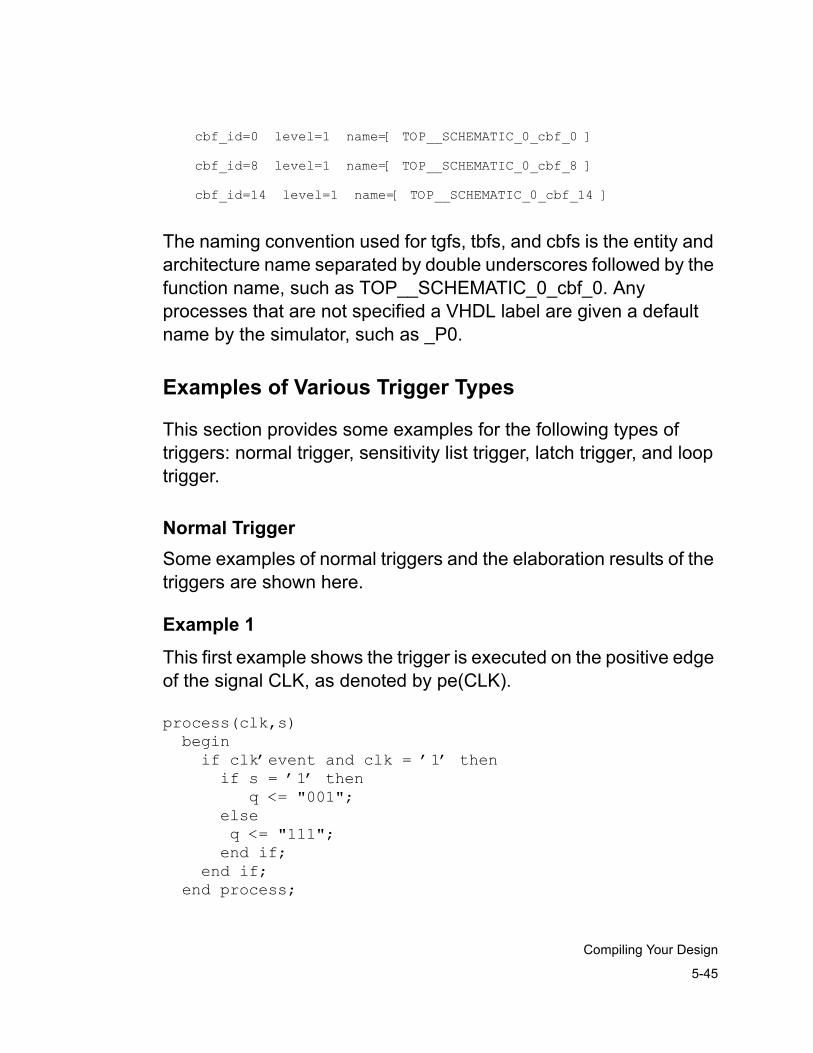
5-45
Compiling Your Design
cbf_id=0 level=1 name=[ TOP__SCHEMATIC_0_cbf_0 ]
cbf_id=8 level=1 name=[ TOP__SCHEMATIC_0_cbf_8 ]
cbf_id=14 level=1 name=[ TOP__SCHEMATIC_0_cbf_14 ]
The naming convention used for tgfs, tbfs, and cbfs is the entity and architecture name separated by double underscores followed by the function name, such as TOP__SCHEMATIC_0_cbf_0. Any processes that are not specified a VHDL label are given a default name by the simulator, such as _P0.
Examples of Various Trigger Types
This section provides some examples for the following types of triggers: normal trigger, sensitivity list trigger, latch trigger, and loop trigger.
Normal TriggerSome examples of normal triggers and the elaboration results of the triggers are shown here.
Example 1
This first example shows the trigger is executed on the positive edge of the signal CLK, as denoted by pe(CLK).
process(clk,s) begin if clk’event and clk = ’1’ then if s = ’1’ then q <= "001"; else q <= "111"; end if; end if; end process;
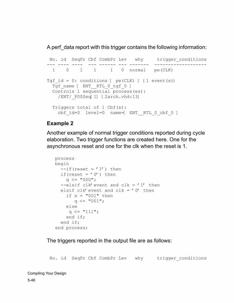
5-46
Compiling Your Design
A perf_data report with this trigger contains the following information:
No. id SeqPr Cbf CombPr Lev why trigger_conditions--- ---- ---- --- ------ --- ------- ------------------- 1 0 1 1 1 0 normal pe(CLK)
Tgf_id = 0: conditions [ pe(CLK) ] {1 event(s)} Tgf_name [ ENT__RTL_0_tgf_0 ] Controls 1 sequential process(es): /ENT/_P0$Seq[1] [2arch.vhd:13]
Triggers total of 1 Cbf(s): cbf_id=0 level=0 name=[ ENT__RTL_0_cbf_0 ]
Example 2
Another example of normal trigger conditions reported during cycle elaboration. Two trigger functions are created here. One for the asynchronous reset and one for the clk when the reset is 1.
process begin --if(reset = ’1’) then if(reset = ’0’) then q <= "000"; --elsif clk’event and clk = ’1’ then elsif clk’event and clk = ’0’ then if s = "001" then q <= "001"; else q <= "111"; end if; end if; end process;
The triggers reported in the output file are as follows:
No. id SeqPr Cbf CombPr Lev why trigger_conditions
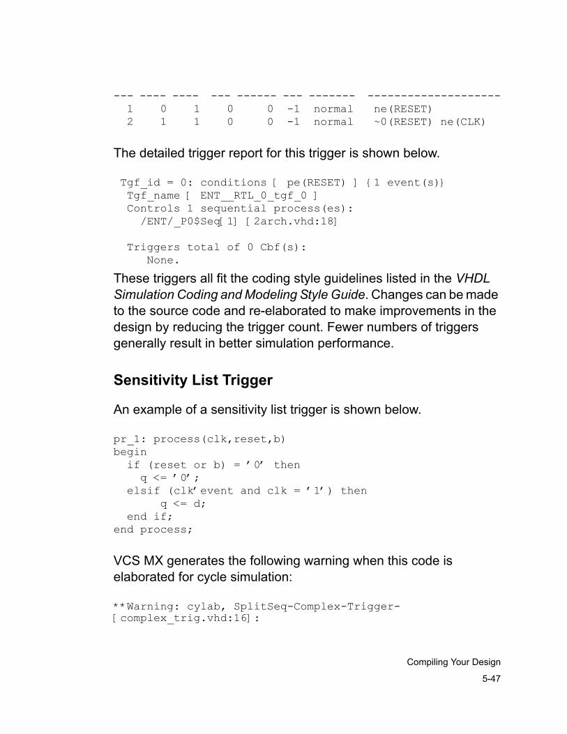
5-47
Compiling Your Design
--- ---- ---- --- ------ --- ------- -------------------- 1 0 1 0 0 -1 normal ne(RESET) 2 1 1 0 0 -1 normal ~0(RESET) ne(CLK)
The detailed trigger report for this trigger is shown below.
Tgf_id = 0: conditions [ pe(RESET) ] {1 event(s)} Tgf_name [ ENT__RTL_0_tgf_0 ] Controls 1 sequential process(es): /ENT/_P0$Seq[1] [2arch.vhd:18]
Triggers total of 0 Cbf(s): None.
These triggers all fit the coding style guidelines listed in the VHDL Simulation Coding and Modeling Style Guide. Changes can be made to the source code and re-elaborated to make improvements in the design by reducing the trigger count. Fewer numbers of triggers generally result in better simulation performance.
Sensitivity List Trigger
An example of a sensitivity list trigger is shown below.
pr_1: process(clk,reset,b)begin if (reset or b) = ’0’ then q <= ’0’; elsif (clk’event and clk = ’1’) then q <= d; end if;end process;
VCS MX generates the following warning when this code is elaborated for cycle simulation:
**Warning: cylab, SplitSeq-Complex-Trigger-[complex_trig.vhd:16]:
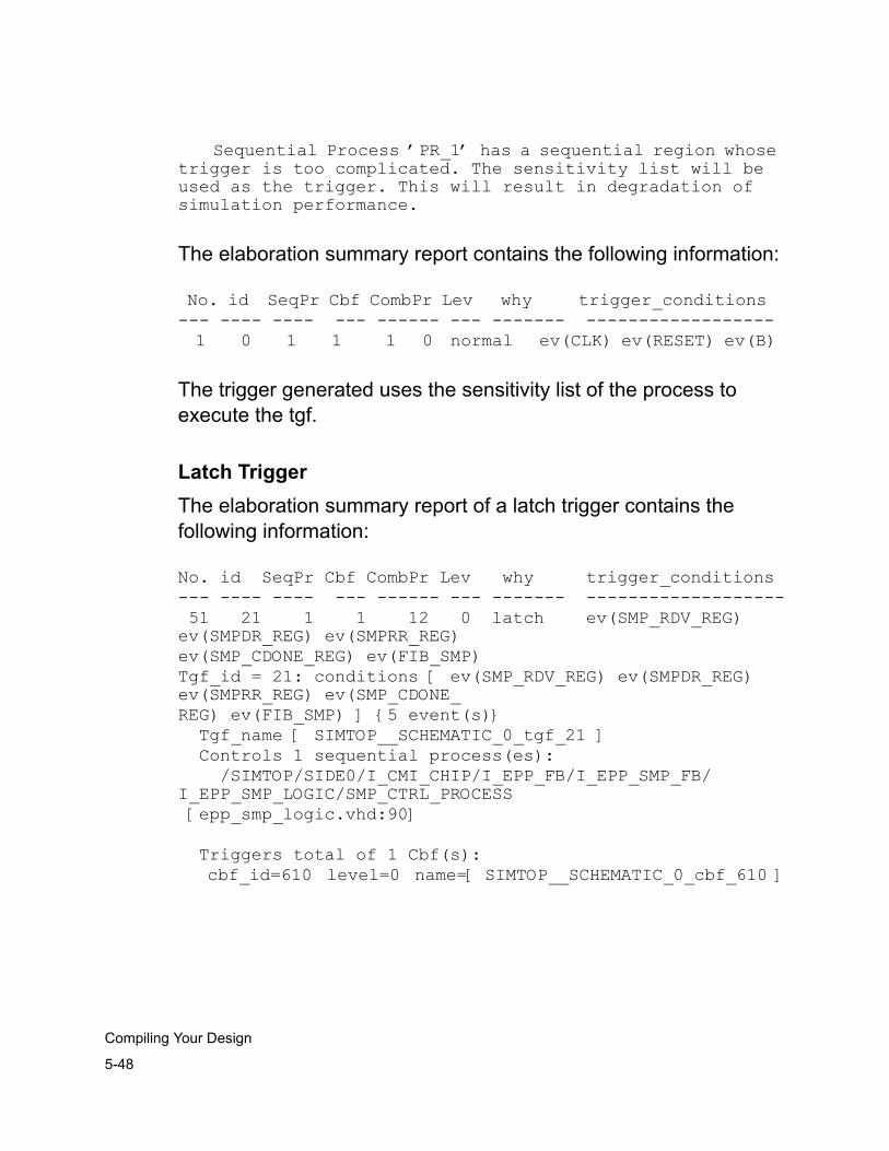
5-48
Compiling Your Design
Sequential Process ’PR_1’ has a sequential region whose trigger is too complicated. The sensitivity list will be used as the trigger. This will result in degradation of simulation performance.
The elaboration summary report contains the following information:
No. id SeqPr Cbf CombPr Lev why trigger_conditions --- ---- ---- --- ------ --- ------- ------------------ 1 0 1 1 1 0 normal ev(CLK) ev(RESET) ev(B)
The trigger generated uses the sensitivity list of the process to execute the tgf.
Latch TriggerThe elaboration summary report of a latch trigger contains the following information:
No. id SeqPr Cbf CombPr Lev why trigger_conditions--- ---- ---- --- ------ --- ------- ------------------- 51 21 1 1 12 0 latch ev(SMP_RDV_REG) ev(SMPDR_REG) ev(SMPRR_REG)ev(SMP_CDONE_REG) ev(FIB_SMP)Tgf_id = 21: conditions [ ev(SMP_RDV_REG) ev(SMPDR_REG) ev(SMPRR_REG) ev(SMP_CDONE_REG) ev(FIB_SMP) ] {5 event(s)} Tgf_name [ SIMTOP__SCHEMATIC_0_tgf_21 ] Controls 1 sequential process(es): /SIMTOP/SIDE0/I_CMI_CHIP/I_EPP_FB/I_EPP_SMP_FB/I_EPP_SMP_LOGIC/SMP_CTRL_PROCESS [epp_smp_logic.vhd:90]
Triggers total of 1 Cbf(s): cbf_id=610 level=0 name=[ SIMTOP__SCHEMATIC_0_cbf_610 ]
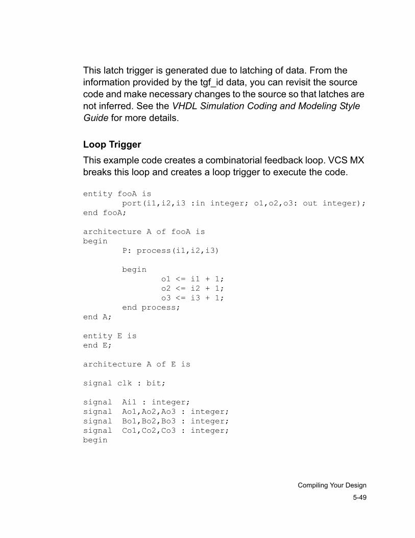
5-49
Compiling Your Design
This latch trigger is generated due to latching of data. From the information provided by the tgf_id data, you can revisit the source code and make necessary changes to the source so that latches are not inferred. See the VHDL Simulation Coding and Modeling Style Guide for more details.
Loop Trigger This example code creates a combinatorial feedback loop. VCS MX breaks this loop and creates a loop trigger to execute the code.
entity fooA is port(i1,i2,i3 :in integer; o1,o2,o3: out integer);end fooA;
architecture A of fooA isbegin P: process(i1,i2,i3)
begin o1 <= i1 + 1; o2 <= i2 + 1; o3 <= i3 + 1; end process;end A;
entity E isend E;
architecture A of E is
signal clk : bit;
signal Ai1 : integer;signal Ao1,Ao2,Ao3 : integer;signal Bo1,Bo2,Bo3 : integer;signal Co1,Co2,Co3 : integer;begin
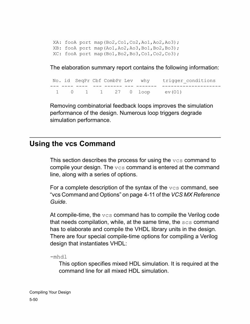
5-50
Compiling Your Design
XA: fooA port map(Bo2,Co1,Co2,Ao1,Ao2,Ao3); XB: fooA port map(Ao1,Ao2,Ao3,Bo1,Bo2,Bo3); XC: fooA port map(Bo1,Bo2,Bo3,Co1,Co2,Co3);
The elaboration summary report contains the following information:
No. id SeqPr Cbf CombPr Lev why trigger_conditions --- ---- ---- --- ------ --- ------- -------------------- 1 0 1 1 27 0 loop ev(O1)
Removing combinatorial feedback loops improves the simulation performance of the design. Numerous loop triggers degrade simulation performance.
Using the vcs Command
This section describes the process for using the vcs command to compile your design. The vcs command is entered at the command line, along with a series of options.
For a complete description of the syntax of the vcs command, see “vcs Command and Options” on page 4-11 of the VCS MX Reference Guide.
At compile-time, the vcs command has to compile the Verilog code that needs compilation, while, at the same time, the scs command has to elaborate and compile the VHDL library units in the design. There are four special compile-time options for compiling a Verilog design that instantiates VHDL:
-mhdlThis option specifies mixed HDL simulation. It is required at the command line for all mixed HDL simulation.
5-51
Compiling Your Design
+vhdllib+logical_libnameThis option specifies the VHDL logical library to use for VHDL design entity instances that you instantiate in your Verilog design. See “Specifying The VHDL Logical Library” on page 4-52.
-vhdlelab "elaboration and compilation command line options"Specifies VCS MX elaboration and compilation options for scs, the VCS MX compiler. In VCS MX VHDL simulation there are three separate steps: analysis, elaboration and compilation (in one step), and simulation. Elaboration and compilation must happen before simulation so VCS starts the scs during Verilog compilation.
+reflib+libSpecifies which logical library to use to resolve Verilog instances instantiated in the VHDL code. By default VCS MX uses all logical libraries with a VERILOG directory in them.
For mixed HDL simulation, you can include all compile-time options on the vcs command line, such as -Mupdate for incremental compilation or -f for specifying a file listing the Verilog source file names for your Verilog design and other compile-time options.
You can include the -R option to begin simulation right after compilation instead of as a separate step, however doing so restricts your ability to specify, through command line options on the simv command line, how to simulate the VHDL part of the design.
Note that multiple Verilog top modules are supported.
5-52
Compiling Your Design
IMPORTANT: For post-processing your design, using DVE or VirSim to view the simulation results, you include the -PP compile-time option. Including the -line compile time option enables line tracing and source debugging. You can also include the +vpdfile+filename compile-time option for specifying the name of the output VCD+ file that DVE or VirSim uses for post-processing.
You can include the -RI option to run VirSim interactively. See “Compiling To Use VirSim Interactively” on page 4-58.
The following is an example of using the -mhdl option with the vcs command:
vcs design.v -Mupdate -line -PP +cli+1 -mhdl
This example contains VCS compile time options: -Mupdate for specifying incremental compilation, -line for enabling stepping through the Verilog code and setting breakpoint in the Verilog code, -PP to compile for post-processing, +cli+1 to see the values of signals, and -mhdl to create a simv executable that can communicate with VCS MX.
Specifying The VHDL Logical Library
You can use the +vhdllib compile-time option to specify the VHDL logical libraries for the VHDL design entity instances that you instantiate in your Verilog design. You use this option if the VHDL logical library isn’t WORK. The format for this options is as follows:
+vhdllib+logical_library_name[+logical_library_name]
5-53
Compiling Your Design
If you are instantiating more than one VHDL design entity and these design entities are from different VHDL logical libraries, you can specify searching both logical libraries, and the order in which to search, to resolve these instances by entering this option more than once.
The following is an example of the use of the +vhdllib option:
vcs design.v -Mupdate -line -PP +cli+1 -mhdl +vhdllib+mylib1 +vhdllib+mylib2
This example specifies resolving VHDL design entity instances by searching VHDL logical libraries mylib1 and mylib2. You can specify the same thing with the following example:
vcs design.v -Mupdate -line -PP +cli+1 -mhdl +vhdllib+mylib1+mylib2
Note: Multiple entries of this option, or specifying multiple logic libraries with this option, also specifies a search order of the logical libraries. If there are design units with the same name in different logical libraries, and you instantiate these design units in your Verilog design and specify the different logical libraries with multiple entries of the +vhdllib compile-time option, these instances are resolved by the first logical library specified with this option.
If you specify the VHDL logical library in the module instantiation statement, this option does not override the logical library specified in the statement.
5-54
Compiling Your Design
Using a Partition File
When you analyzed the source code, you had the option of analyzing the design units in some or all of the source files to enable them to be compiled for cycle-based mode (with the -cycle vhdlan command line option). If you did you can now have these design units compiled for cycle-based mode.You do this with a partition file.
In the partition file you specify design entities either by their entity name or their configuration and whether all instances of them, and unless otherwise specified all design entities hierarchically under the specified design entities, simulate in cycle-based mode instead of the default event-driven mode.
If you want some design entities that are instantiated lower in the hierarchy to simulate in event-driven mode (for debugging) you can specify that all instances of these design entities, and all those hierarchically under them, simulate in event-driven mode with similar entries in the partition file.
The format of a line in the partition file is as follows:
cycle | event entity_name | configuration_name
Consider the example in Figure 5-17:
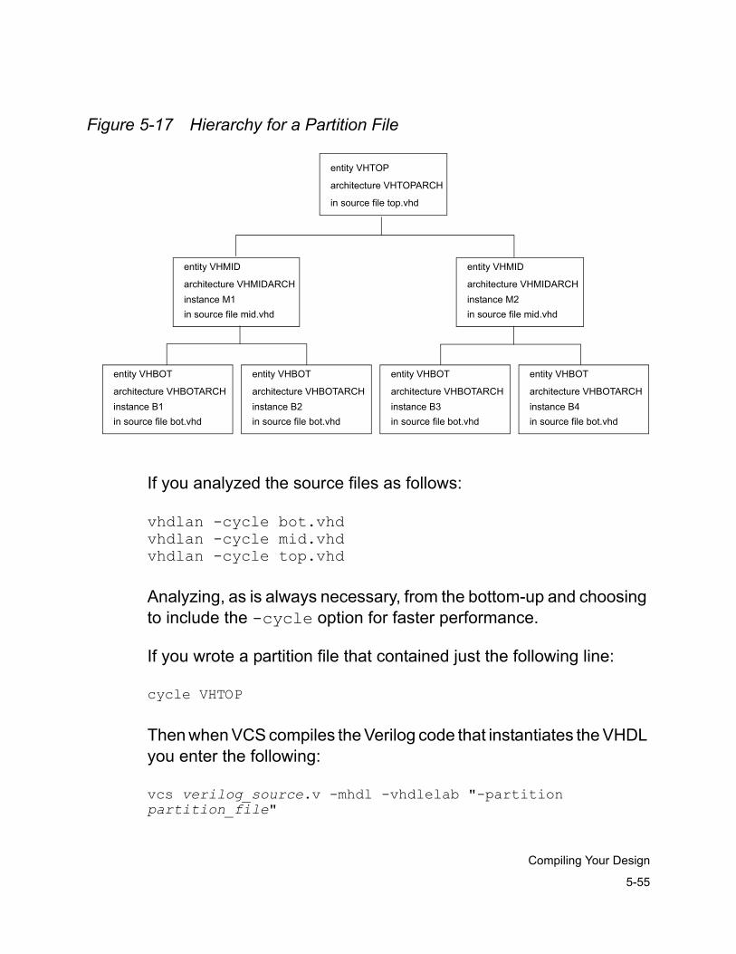
5-55
Compiling Your Design
Figure 5-17 Hierarchy for a Partition File
If you analyzed the source files as follows:
vhdlan -cycle bot.vhdvhdlan -cycle mid.vhdvhdlan -cycle top.vhd
Analyzing, as is always necessary, from the bottom-up and choosing to include the -cycle option for faster performance.
If you wrote a partition file that contained just the following line:
cycle VHTOP
Then when VCS compiles the Verilog code that instantiates the VHDL you enter the following:
vcs verilog_source.v -mhdl -vhdlelab "-partition partition_file"
entity VHTOP
architecture VHTOPARCH
in source file top.vhd
entity VHMID
architecture VHMIDARCH
in source file mid.vhdinstance M1
entity VHMID
architecture VHMIDARCH
in source file mid.vhdinstance M2
entity VHBOT
architecture VHBOTARCH
in source file bot.vhdinstance B1
entity VHBOT
architecture VHBOTARCH
in source file bot.vhdinstance B2
entity VHBOT
architecture VHBOTARCH
in source file bot.vhdinstance B3
entity VHBOT
architecture VHBOTARCH
in source file bot.vhdinstance B4
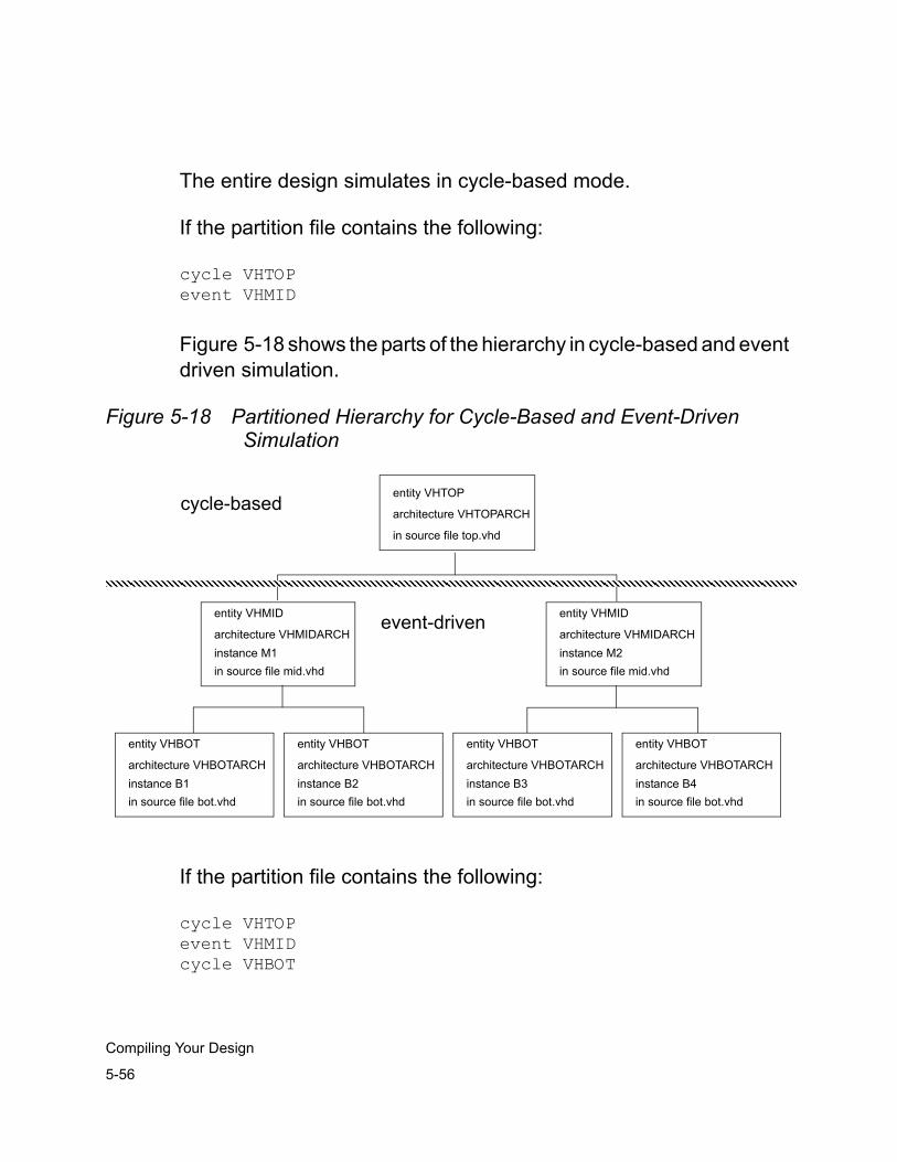
5-56
Compiling Your Design
The entire design simulates in cycle-based mode.
If the partition file contains the following:
cycle VHTOPevent VHMID
Figure 5-18 shows the parts of the hierarchy in cycle-based and event driven simulation.
Figure 5-18 Partitioned Hierarchy for Cycle-Based and Event-Driven Simulation
If the partition file contains the following:
cycle VHTOPevent VHMIDcycle VHBOT
entity VHTOP
architecture VHTOPARCH
in source file top.vhd
entity VHMID
architecture VHMIDARCH
in source file mid.vhdinstance M1
entity VHMID
architecture VHMIDARCH
in source file mid.vhdinstance M2
entity VHBOT
architecture VHBOTARCH
in source file bot.vhdinstance B1
entity VHBOT
architecture VHBOTARCH
in source file bot.vhdinstance B2
entity VHBOT
architecture VHBOTARCH
in source file bot.vhdinstance B3
entity VHBOT
architecture VHBOTARCH
in source file bot.vhdinstance B4
cycle-based
event-driven
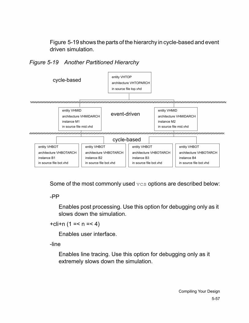
5-57
Compiling Your Design
Figure 5-19 shows the parts of the hierarchy in cycle-based and event driven simulation.
Figure 5-19 Another Partitioned Hierarchy
Some of the most commonly used vcs options are described below:
-PP
Enables post processing. Use this option for debugging only as it slows down the simulation.
+cli+n (1 =< n =< 4)
Enables user interface.
-line
Enables line tracing. Use this option for debugging only as it extremely slows down the simulation.
entity VHTOP
architecture VHTOPARCH
in source file top.vhd
entity VHMID
architecture VHMIDARCH
in source file mid.vhdinstance M1
entity VHMID
architecture VHMIDARCH
in source file mid.vhdinstance M2
entity VHBOT
architecture VHBOTARCH
in source file bot.vhdinstance B1
entity VHBOT
architecture VHBOTARCH
in source file bot.vhdinstance B2
entity VHBOT
architecture VHBOTARCH
in source file bot.vhdinstance B3
entity VHBOT
architecture VHBOTARCH
in source file bot.vhdinstance B4
cycle-based
event-driven
cycle-based
5-58
Compiling Your Design
+vcsd
Enables the Direct PLI interface.
+rad
Enables Radiant optimizations
+race
Enables “race” report generation
+notimingchecks
Specifies no timing simulation (used for parsing only)
+nospecify
Specifies no path delays (used for parsing only)
Compiling To Use VirSim Interactively
You can use VirSim interactively to debug the entire mixed HDL design.
To use VirSim for interactive debugging include the -RI option on the vcs command line just like you would for an entirely Verilog design. This option starts the simulation and VirSim right after compilation. There is however the following restriction: Do not include the -PP or -I option to enable post-processing.
IMPORTANT:
• When you start VirSim for interactive simulation There is no way that you can enter scsim command line options to tell VCS MX how to simulate the VHDL part of the design.
• You can enter these commands on the simv command line but you can’t start VirSim with an option on the simv command line.
5-59
Compiling Your Design
• If you need to both interactively simulate with VirSim and also enter scsim command line options, you will need to interactively simulate your design twice.
When simulation starts the VirSim windows will display both the Verilog and VHDL parts of the design. You can enter CLI commands in the Command field of the Interactive window that apply to both the Verilog and VHDL part of the design.
Common Verilog Compilation Tasks
This section outlines some of the common tasks performed by the vcs command.
Save and Restart
VCS provides a save and restart feature that allows checkpoints of the simulation to be saved at arbitrary times. The resulting checkpoint files can be executed at a later time, causing simulation to resume at the point immediately following the save.
Note: Save and restart is not supported on Windows.
Benefits of save and restart include:
• Regular checkpoints for interactively debugging problems found during long batch runs
• Use of plusargs to start action such as $dumpvars on restart
• Executes common simulation system tasks such as $reset just once in a regression
Restrictions of save and restart include:
5-60
Compiling Your Design
• Requires extra Verilog code to manage the save and restart
• Must duplicate start-up code if handling plusargs on restart
• File I/O suspend and resume in PLI applications must be given special consideration
Save and Restart ExampleA simple example of save and restart is given below to demonstrate the basic functionality.
The $save call does not execute a save immediately, but schedules the checkpoint save at the end of the current simulation time just before events scheduled with #0 are processed. Therefore, events delayed with #0 are the first to be processed upon restart.
% cat test.vmodule simple_restart;initial begin
#10$display("one");$save("test.chk");$display("two");#0 // make the following occur at restart$display("three");#10$display("four");
endendmodule
Now to compile the example Source file:
vcs -Mupdate test.v
Now run the simulation:
simv
5-61
Compiling Your Design
VCS displays the following:
onetwo$save: Creating test.chk from current state of simv...threefour
Now to restart the simulation from the state saved in the check file, enter:
test.chk
VCS displays the following:
Restart of a saved simulationthreefour
Save and Restart File I/O
VCS MX remembers the files you opened via $fopen and reopens them when you restart the simulation. If no file exists having the old filename, VCS MX opens a new file with the old filename. If a file exists having the same name and length at time of save as the old file, then VCS MX appends further output to that file. Otherwise, VCS attempts to open a file with filename equal to the old filename plus the suffix .N. If a file with this name exists, VCS exits with an error.
If your simulation contains PLI routines that do file I/O, the routines must detect both the save and restart events, closing and reopening files as needed. You can detect save and restart calls using misctf callbacks with reasons reason_save and reason_restart.
5-62
Compiling Your Design
When running the saved checkpoint file, be sure to rename it so that further $save calls do not overwrite the binary you are running. There is no way from within the Verilog source code to determine if you are in a previously saved and restarted simulation, so you cannot suppress the $save calls in a restarted binary.
Save and Restart with Runtime Options
If your simulation behavior depends on the existence of run-time plusargs or any other run-time action (such as reading a vector file), be aware that the restarted simulation uses the values from the original run unless you add special code to process run-time events after the restart action. Depending on the complexity of your environment and your usage of the save and restart feature, this can be a significant task.
For example, if you load a memory image with $loadmemb at the beginning of the simulation and want to be able to restart from a checkpoint with a different memory image, you must add Verilog code to load the memory image after every $save call. This ensures that at the beginning of any restart the correct memory image is loaded before simulation begins. A reasonable way to manage this is to create a task to handle processing arguments, and call this task at the start of execution, and after each save.
A more detailed example follows to illustrate this. The first run optimizes simulation speed by omitting the +dump flag. If a bug is found, the latest checkpoint file is run with the +dump flag to enable signal dumping.
// file test.vmodule dumpvars();task processargs;
beginif ($test$plusargs("dump")) begin
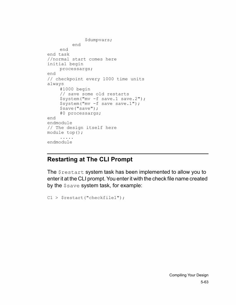
5-63
Compiling Your Design
$dumpvars;end
endend task//normal start comes hereinitial begin
processargs;end// checkpoint every 1000 time units always
#1000 begin// save some old restarts$system("mv -f save.1 save.2");$system("mv -f save save.1");$save("save");#0 processargs;
endendmodule// The design itself heremodule top();
.....endmodule
Restarting at The CLI Prompt
The $restart system task has been implemented to allow you to enter it at the CLI prompt. You enter it with the check file name created by the $save system task, for example:
C1 > $restart("checkfile1");
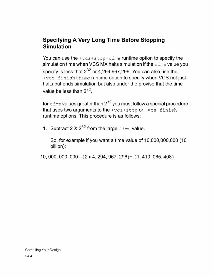
5-64
Compiling Your Design
Specifying A Very Long Time Before Stopping Simulation
You can use the +vcs+stop+time runtime option to specify the simulation time when VCS MX halts simulation if the time value you specify is less that 232 or 4,294,967,296. You can also use the +vcs+finish+time runtime option to specify when VCS not just halts but ends simulation but also under the proviso that the time value be less than 232.
for time values greater than 232 you must follow a special procedure that uses two arguments to the +vcs+stop or +vcs+finish runtime options. This procedure is as follows:
1. Subtract 2 X 232 from the large time value.
So, for example if you want a time value of 10,000,000,000 (10 billion):
10 000 000 000, , , 2 4 294 967 296, , ,•( ) 1 410 065 408, , ,( )=–
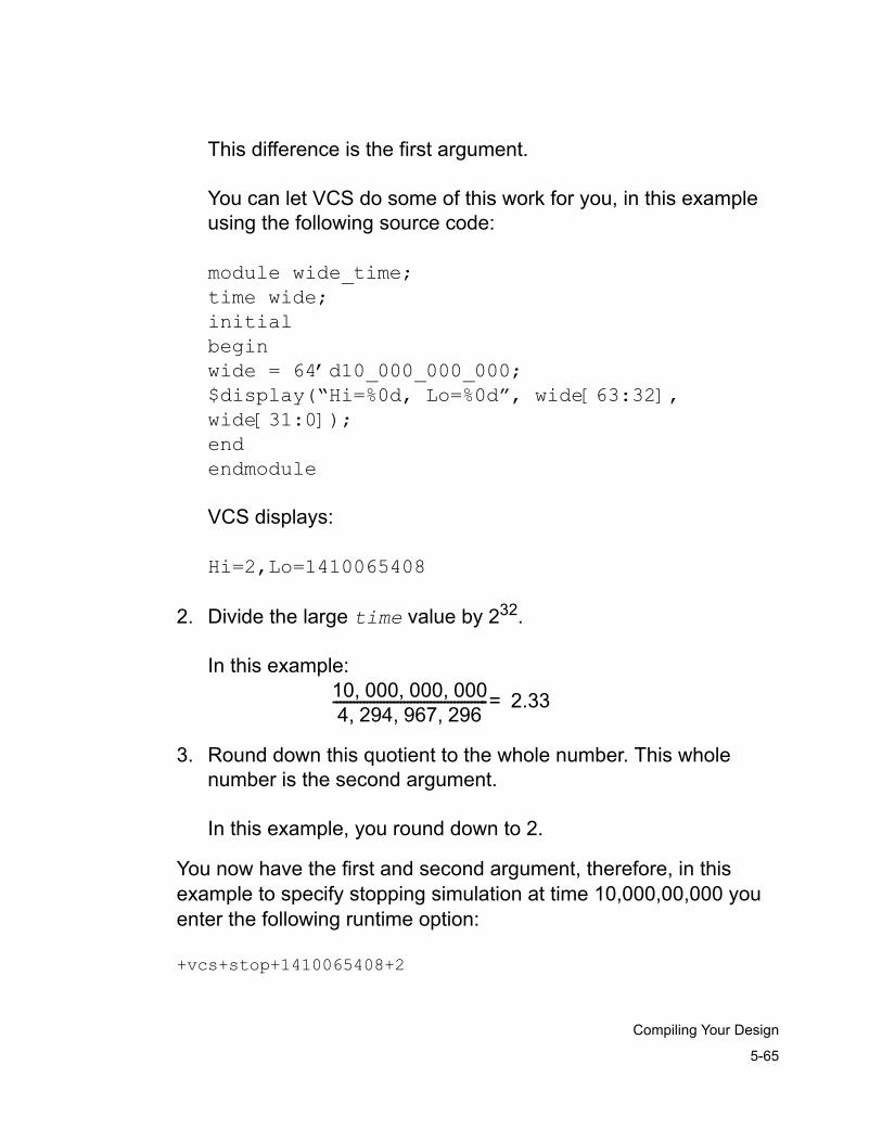
5-65
Compiling Your Design
This difference is the first argument.
You can let VCS do some of this work for you, in this example using the following source code:
module wide_time;time wide;initialbeginwide = 64’d10_000_000_000;$display(“Hi=%0d, Lo=%0d”, wide[63:32], wide[31:0]);endendmodule
VCS displays:
Hi=2,Lo=1410065408
2. Divide the large time value by 232.
In this example:
3. Round down this quotient to the whole number. This whole number is the second argument.
In this example, you round down to 2.
You now have the first and second argument, therefore, in this example to specify stopping simulation at time 10,000,00,000 you enter the following runtime option:
+vcs+stop+1410065408+2
10 000 000 000, , ,4 294 967 296, , ,---------------------------------------------- 2.33=
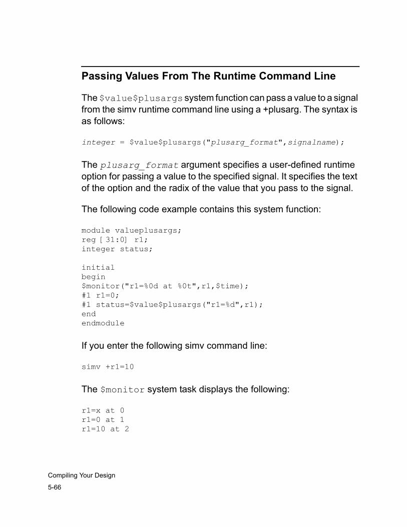
5-66
Compiling Your Design
Passing Values From The Runtime Command Line
The $value$plusargs system function can pass a value to a signal from the simv runtime command line using a +plusarg. The syntax is as follows:
integer = $value$plusargs("plusarg_format",signalname);
The plusarg_format argument specifies a user-defined runtime option for passing a value to the specified signal. It specifies the text of the option and the radix of the value that you pass to the signal.
The following code example contains this system function:
module valueplusargs;reg [31:0] r1;integer status;
initialbegin$monitor("r1=%0d at %0t",r1,$time);#1 r1=0;#1 status=$value$plusargs("r1=%d",r1);endendmodule
If you enter the following simv command line:
simv +r1=10
The $monitor system task displays the following:
r1=x at 0r1=0 at 1r1=10 at 2
5-67
Compiling Your Design
Performance Considerations
When you simulate your design you can look for ways to improve the simulation performance. There are run-time options that enable VCS to simulate faster or slower. There is also a technique called profiling that tells you which modules in your design take the most CPU time.
Runtime Options that Accelerate or Impede Simulation
Some runtime options enable VCS MX to simulate your design faster because they allow VCS MX to skip certain operations. You should consider using these run-time options. These runtime options are as follows:
+vcs+dumpvarsoff Suppress $dumpvars system tasks.
+vcs+ignorestop Tells VCS to ignore the $stop system tasks in your source code.
+notimingcheck Disables timing check system tasks. Using this option at compile-time results in even faster simulation than using it at runtime.
The run-time options that specify writing to a file that slow down simulation. These run-time options are as follows:
-a filename All output of simulation is appended to filename as well as sent to the standard output.
-l filename All output of simulation is written to filename as well as to the standard output.
Other run-time options that specify operations other than the default operations also slow down simulation to some extent.
5-68
Compiling Your Design
Profiling the Simulation
If you include the +prof compile-time option when you compile your design, VCS MX generates the vcs.prof file during simulation. This file contains a profile of the simulation. It reports the following:
• The module instances in the hierarchy that use the most CPU time
• The module definitions whose instances use the most CPU time
• The Verilog constructs in those instances that use the most CPU time
You can use this information to see where in your design you might be able to modify your code for faster simulation performance.
The profile data in the vcs.prof file is organized into a number of “views” of the simulation. They are as follows:
• Top Level View
• Module View
• Instance View
• Module Construct Mapping View
• Top Level Construct View
• Construct View Across Design
The Top Level View
This view shows you how much CPU time was used by:
• Any PLI application that executes along with VCS
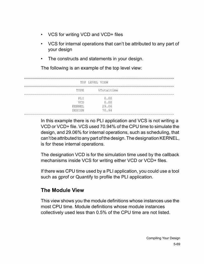
5-69
Compiling Your Design
• VCS for writing VCD and VCD+ files
• VCS for internal operations that can’t be attributed to any part of your design
• The constructs and statements in your design.
The following is an example of the top level view:
=========================================================================== TOP LEVEL VIEW =========================================================================== TYPE %Totaltime--------------------------------------------------------------------------- PLI 0.00 VCD 0.00 KERNEL 29.06 DESIGN 70.94---------------------------------------------------------------------------
In this example there is no PLI application and VCS is not writing a VCD or VCD+ file. VCS used 70.94% of the CPU time to simulate the design, and 29.06% for internal operations, such as scheduling, that can’t be attributed to any part of the design. The designation KERNEL, is for these internal operations.
The designation VCD is for the simulation time used by the callback mechanisms inside VCS for writing either VCD or VCD+ files.
If there was CPU time used by a PLI application, you could use a tool such as gprof or Quantify to profile the PLI application.
The Module View
This view shows you the module definitions whose instances use the most CPU time. Module definitions whose module instances collectively used less than 0.5% of the CPU time are not listed.
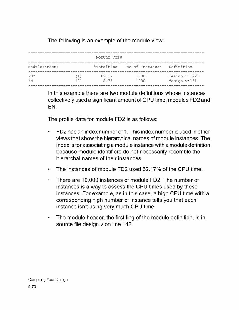
5-70
Compiling Your Design
The following is an example of the module view:
=========================================================================== MODULE VIEW===========================================================================Module(index) %Totaltime No of Instances Definition---------------------------------------------------------------------------FD2 (1) 62.17 10000 design.v:142.EN (2) 8.73 1000 design.v:131.---------------------------------------------------------------------------
In this example there are two module definitions whose instances collectively used a significant amount of CPU time, modules FD2 and EN.
The profile data for module FD2 is as follows:
• FD2 has an index number of 1. This index number is used in other views that show the hierarchical names of module instances. The index is for associating a module instance with a module definition because module identifiers do not necessarily resemble the hierarchal names of their instances.
• The instances of module FD2 used 62.17% of the CPU time.
• There are 10,000 instances of module FD2. The number of instances is a way to assess the CPU times used by these instances. For example, as in this case, a high CPU time with a corresponding high number of instance tells you that each instance isn’t using very much CPU time.
• The module header, the first ling of the module definition, is in source file design.v on line 142.

5-71
Compiling Your Design
The Instance View
This view shows you the module instances that use the most CPU time. An instance must use more than 0.5% of the CPU time to be entered in this view.
The following is an example of the instance view:
=========================================================================== INSTANCE VIEW===========================================================================Instance %Totaltime---------------------------------------------------------------------------test.lfsr1000_1.lfsr100_1.lfsr10_1.lfsr_1.en_1 ( 2 ) 0.73
---------------------------------------------------------------------------
In this example there is only one instance that uses more that 0.5% of the CPU time.
This instance’s hierarchical name is test.lfsr1000_1.lfsr100_1.lfsr10_1.lfsr_1.en_1. Long hierarchical names wrap to the next line.
The instance’s index number is 2, indication that it is an instance of module EN, which had an index of 2 in the module view.
This instance used 0.73% of the CPU time.
No instance of module FD2 is listed here so no individual instance of FD2 used more that 0.5% of the CPU time.
Note: It is very common for no instances to appear in the instance view. This happens when many instances use some of the simulation time but none use more than 0.5% of the total simulation time.
5-72
Compiling Your Design
The Module to Construct Mapping View
This view shows you the CPU time used by different types of Verilog constructs in each module definition in the module view. There are the following types of Verilog constructs:
• always constructs (commonly called always blocks)
• initial constructs (commonly called initial blocks)
• module path delays in specify blocks
• timing check system tasks in specify blocks
• combinational logic including gates or built-in primitives and continuous assignment statements
• user-defined tasks
• user-defined functions
• module instance ports
• user-defined primitives (UDPs)
• Any Verilog code protected by encryption
Ports use simulation time particularly when there are expressions in port connection lists such as bit or part selects and concatenation operators.
This view has separate sections for the Verilog constructs for each module definition in the module view.
The following is an example of a module to construct mapping view:
=========================================================================== MODULE TO CONSTRUCT MAPPING===========================================================================
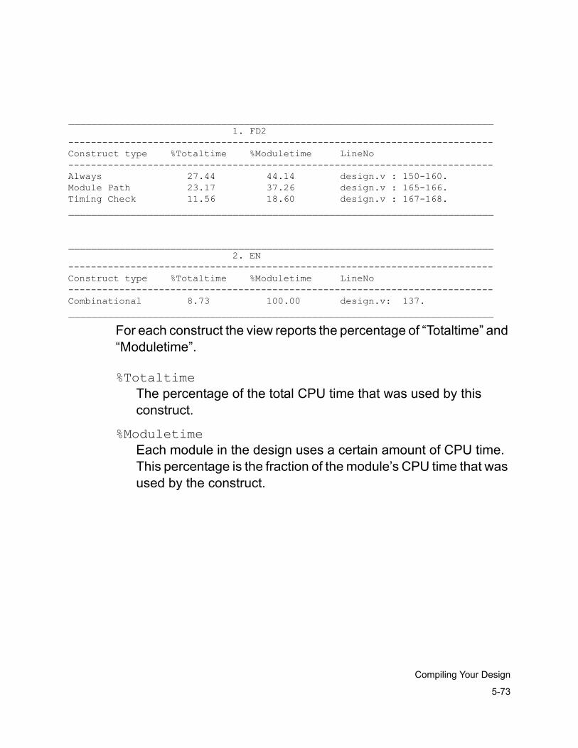
5-73
Compiling Your Design
___________________________________________________________________________ 1. FD2---------------------------------------------------------------------------Construct type %Totaltime %Moduletime LineNo---------------------------------------------------------------------------Always 27.44 44.14 design.v : 150-160.Module Path 23.17 37.26 design.v : 165-166.Timing Check 11.56 18.60 design.v : 167-168.___________________________________________________________________________
___________________________________________________________________________ 2. EN---------------------------------------------------------------------------Construct type %Totaltime %Moduletime LineNo---------------------------------------------------------------------------Combinational 8.73 100.00 design.v: 137.___________________________________________________________________________
For each construct the view reports the percentage of “Totaltime” and “Moduletime”.
%TotaltimeThe percentage of the total CPU time that was used by this construct.
%ModuletimeEach module in the design uses a certain amount of CPU time. This percentage is the fraction of the module’s CPU time that was used by the construct.
5-74
Compiling Your Design
In the section for module FD2:
• An always block in this module definition used 27.44% of the TOTAL CPU time. Of all the CPU time consumed by all instances of the FD2 module, 44.14% is spent on this construct (44.14% of 62.17% = 27.44%). The always block is in source file design.v between lines 150 and 160.
If there were another always block in module FD2 that used more than 0.5% of the CPU time, there would be another line in this section for it, beginning with the always keyword.
• The module path delays in this module used 23.17% of the TOTAL CPU time. Of all the CPU time consumed by all instances of the FD2 module, 37.26% is spent on this construct. These module path delays can be found on lines 165-166 of the design.v source file.
• The timing check system tasks in this module used 11.56% of the TOTAL CPU time. Of all the CPU time consumed by all instances of the FD2 module, 18.60% is spent on this construct. These timing check system tasks can be found on lines 167-167 of the design.v source file.
In the section for module EN, a construct classified as Combinational used 8.73 of the total CPU time. 100% of the CPU time used by all instances of EN were used for this combinational construct.
No initial blocks, user-defined functions, or user-defined tasks, ports, UDPs, or encrypted code in the design used more than 0.5% of the CPU time. If there were, there would be a separate line for each of these types of constructs.
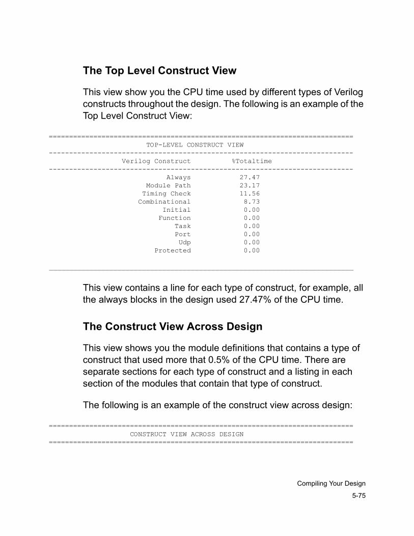
5-75
Compiling Your Design
The Top Level Construct View
This view show you the CPU time used by different types of Verilog constructs throughout the design. The following is an example of the Top Level Construct View:
=========================================================================== TOP-LEVEL CONSTRUCT VIEW--------------------------------------------------------------------------- Verilog Construct %Totaltime--------------------------------------------------------------------------- Always 27.47 Module Path 23.17 Timing Check 11.56 Combinational 8.73 Initial 0.00 Function 0.00 Task 0.00 Port 0.00 Udp 0.00 Protected 0.00
___________________________________________________________________________
This view contains a line for each type of construct, for example, all the always blocks in the design used 27.47% of the CPU time.
The Construct View Across Design
This view shows you the module definitions that contains a type of construct that used more that 0.5% of the CPU time. There are separate sections for each type of construct and a listing in each section of the modules that contain that type of construct.
The following is an example of the construct view across design:
=========================================================================== CONSTRUCT VIEW ACROSS DESIGN===========================================================================
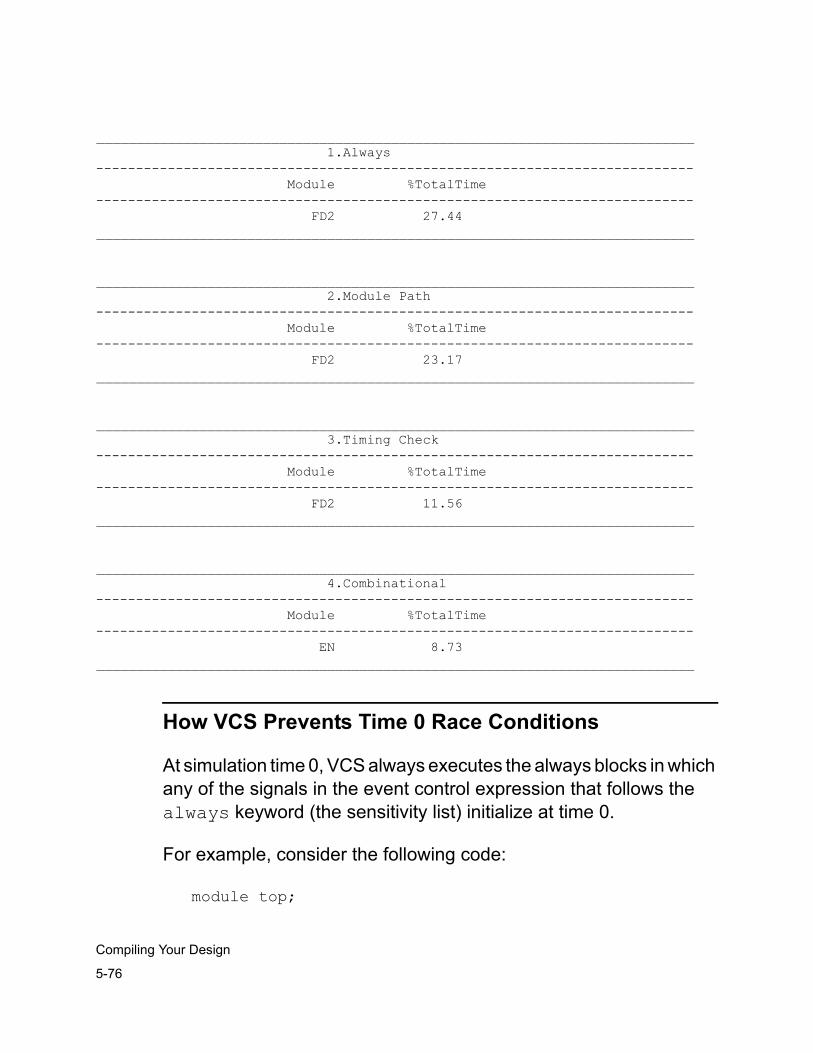
5-76
Compiling Your Design
___________________________________________________________________________ 1.Always--------------------------------------------------------------------------- Module %TotalTime--------------------------------------------------------------------------- FD2 27.44___________________________________________________________________________
___________________________________________________________________________ 2.Module Path--------------------------------------------------------------------------- Module %TotalTime--------------------------------------------------------------------------- FD2 23.17___________________________________________________________________________
___________________________________________________________________________ 3.Timing Check--------------------------------------------------------------------------- Module %TotalTime--------------------------------------------------------------------------- FD2 11.56___________________________________________________________________________
___________________________________________________________________________ 4.Combinational--------------------------------------------------------------------------- Module %TotalTime--------------------------------------------------------------------------- EN 8.73___________________________________________________________________________
How VCS Prevents Time 0 Race Conditions
At simulation time 0, VCS always executes the always blocks in which any of the signals in the event control expression that follows the always keyword (the sensitivity list) initialize at time 0.
For example, consider the following code:
module top;
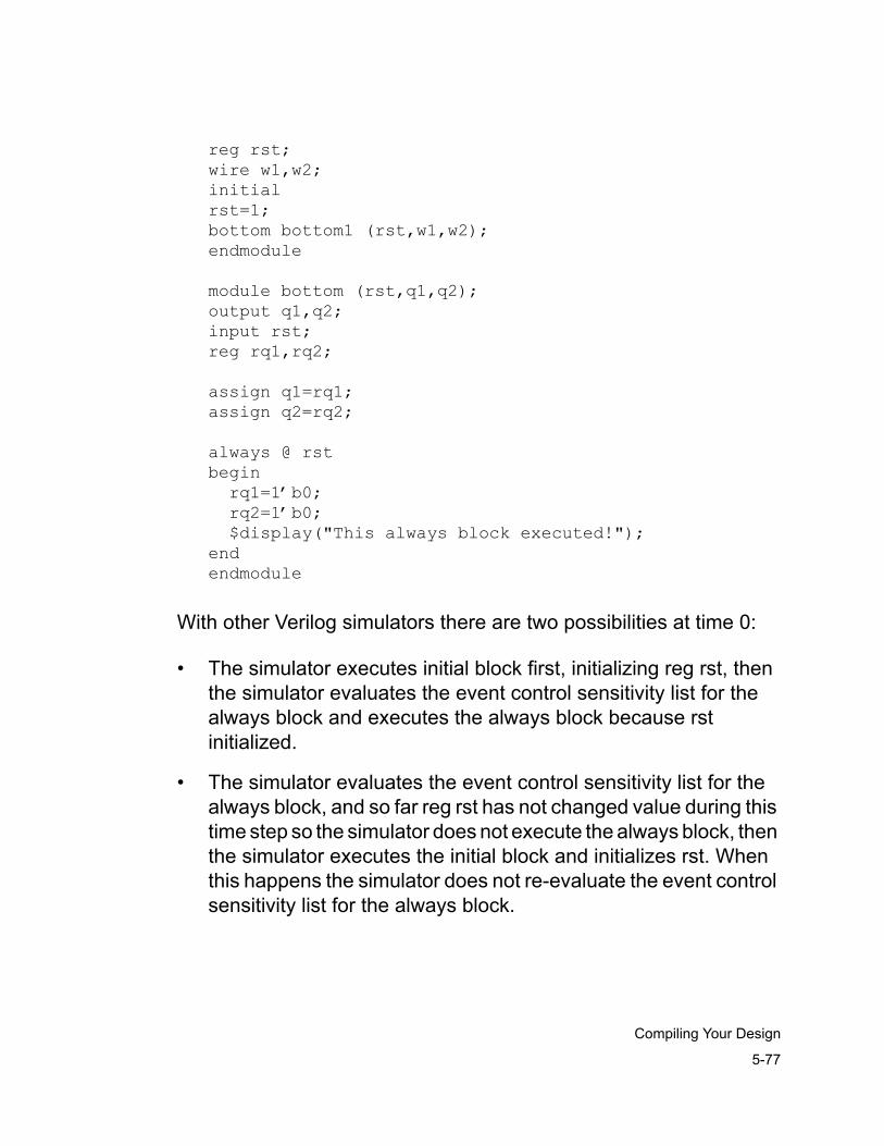
5-77
Compiling Your Design
reg rst;wire w1,w2;initialrst=1;bottom bottom1 (rst,w1,w2);endmodule
module bottom (rst,q1,q2);output q1,q2;input rst;reg rq1,rq2;
assign q1=rq1;assign q2=rq2;
always @ rstbegin rq1=1’b0; rq2=1’b0; $display("This always block executed!");endendmodule
With other Verilog simulators there are two possibilities at time 0:
• The simulator executes initial block first, initializing reg rst, then the simulator evaluates the event control sensitivity list for the always block and executes the always block because rst initialized.
• The simulator evaluates the event control sensitivity list for the always block, and so far reg rst has not changed value during this time step so the simulator does not execute the always block, then the simulator executes the initial block and initializes rst. When this happens the simulator does not re-evaluate the event control sensitivity list for the always block.

5-78
Compiling Your Design
Compiling and Elaborating Verilog in a Mixed-HDL Design
VCS MX supports VCS compilation options for controlling the compilation Verilog portion of a mixed-HDL design. For default compilation of Verilog portion (default performance, no debugging or post-processing capabilities), you can use -mhdl switch at the scs command line instead of -verilogcomp “ “.
In case you wish to get more performance or enable interactive or post-processing debug capabilities, you need to specify additional Verilog compilation/code generation options. You can specify all of them through the -verilogcomp option. You can specify one or multiple options between quotation marks. The syntax is -
% scs LIB.cfg -mhdl
Or
% scs LIB.cfg -verilogcomp “VCS_code-gen_options”
More examples,
% scs lib.cfg_design -mhdl % scs lib.cfg_design -verilogcomp “+rad”% scs lib.cfg_design -verilogcomp “-PP”
In this step, Verilog portion of the design is compiled and the full design is elaborated. Errors in Verilog compilation and full design elaboration are reported. You must fix the errors in case they occur.
By default, eight language layers of VHDL/Verilog are supported. In case your design has more language layers than eight, use -maxLayers option to increase the language layers. For example -
5-79
Compiling Your Design
% scs LIB.cfg -maxLayers 10 -mhdl
Note:Ideally, you should not use any Verilog parsing or reference resolving options and Verilog source files through -verilogcomp. But, if you are an advanced mixed language simulation user, and in case you want to provide all the Verilog source files during actual code-generation time, you can pass them within -verilogcomp option. This will have higher precedence over the already parsed Verilog source files. We do not encourage using this feature in normal circumstances as there is a probability of wrong modules getting picked up resulting in incorrect simulation,
Resolving References
By default, elaboration will look into WORK library for resolving VHDL and Verilog references within Verilog modules.
Elaboration also automatically searches all the logical libraries in the order they are specified in the synopsys_sim.setup file to resolve references.
Note:This may sometimes result into wrong design units getting picked up automatically from wrong libraries. If you suspect that you are running into this case, consider using the options +vhdllib+LIB and +reflib+LIB either during vlogan (along with -resolve) or within -verilogcomp.

5-80
Compiling Your Design
6-1
Getting Started
6VCS MX Flow Examples 1
This chapter provides the following:
• VHDL-Top Mixed Language Flow Example
• Verilog-Top Mixed Language Flow Example
• VCS MX Flows at a Glance
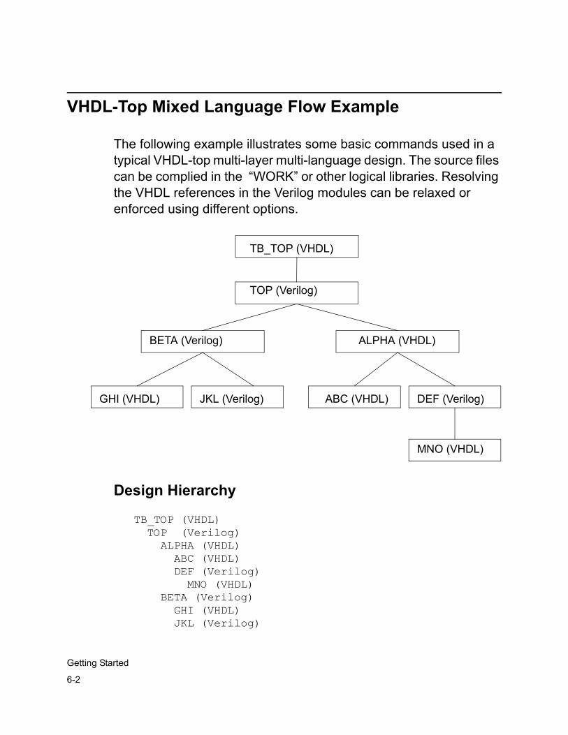
6-2
Getting Started
VHDL-Top Mixed Language Flow Example
The following example illustrates some basic commands used in a typical VHDL-top multi-layer multi-language design. The source files can be complied in the “WORK” or other logical libraries. Resolving the VHDL references in the Verilog modules can be relaxed or enforced using different options.
Design Hierarchy
TB_TOP (VHDL) TOP (Verilog) ALPHA (VHDL) ABC (VHDL) DEF (Verilog) MNO (VHDL) BETA (Verilog) GHI (VHDL) JKL (Verilog)
TB_TOP (VHDL)
TOP (Verilog)
ALPHA (VHDL)
ABC (VHDL) DEF (Verilog)
MNO (VHDL)
BETA (Verilog)
GHI (VHDL) JKL (Verilog)
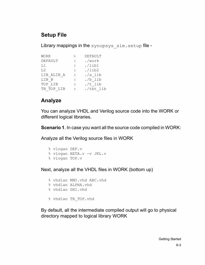
6-3
Getting Started
Setup File
Library mappings in the synopsys_sim.setup file -
WORK > DEFAULTDEFAULT : ./workL1 : ./lib1L2 : ./lib2LIB_ALIB_A : ./a_libLIB_B : ./b_libTOP_LIB : ./t_libTB_TOP_LIB : ./tbt_lib
Analyze
You can analyze VHDL and Verilog source code into the WORK or different logical libraries.
Scenario 1. In case you want all the source code compiled in WORK:
Analyze all the Verilog source files in WORK
% vlogan DEF.v% vlogan BETA.v -v JKL.v% vlogan TOP.v
Next, analyze all the VHDL files in WORK (bottom up)
% vhdlan MNO.vhd ABC.vhd% vhdlan ALPHA.vhd% vhdlan GHI.vhd
% vhdlan TB_TOP.vhd
By default, all the intermediate compiled output will go to physical directory mapped to logical library WORK
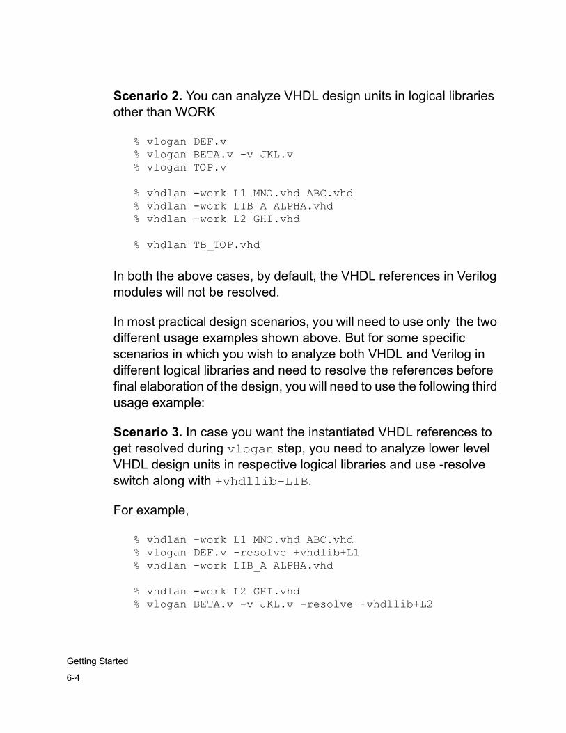
6-4
Getting Started
Scenario 2. You can analyze VHDL design units in logical libraries other than WORK
% vlogan DEF.v% vlogan BETA.v -v JKL.v% vlogan TOP.v
% vhdlan -work L1 MNO.vhd ABC.vhd% vhdlan -work LIB_A ALPHA.vhd% vhdlan -work L2 GHI.vhd
% vhdlan TB_TOP.vhd
In both the above cases, by default, the VHDL references in Verilog modules will not be resolved.
In most practical design scenarios, you will need to use only the two different usage examples shown above. But for some specific scenarios in which you wish to analyze both VHDL and Verilog in different logical libraries and need to resolve the references before final elaboration of the design, you will need to use the following third usage example:
Scenario 3. In case you want the instantiated VHDL references to get resolved during vlogan step, you need to analyze lower level VHDL design units in respective logical libraries and use -resolve switch along with +vhdllib+LIB.
For example,
% vhdlan -work L1 MNO.vhd ABC.vhd% vlogan DEF.v -resolve +vhdlib+L1% vhdlan -work LIB_A ALPHA.vhd
% vhdlan -work L2 GHI.vhd% vlogan BETA.v -v JKL.v -resolve +vhdllib+L2
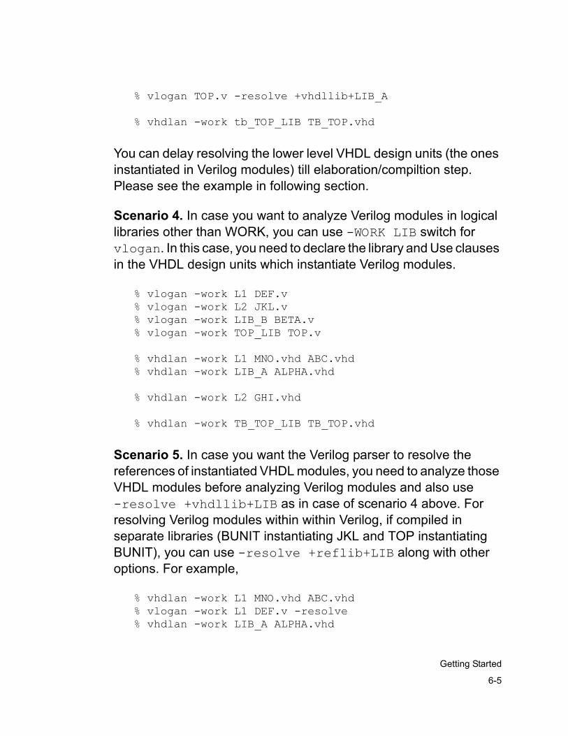
6-5
Getting Started
% vlogan TOP.v -resolve +vhdllib+LIB_A
% vhdlan -work tb_TOP_LIB TB_TOP.vhd
You can delay resolving the lower level VHDL design units (the ones instantiated in Verilog modules) till elaboration/compiltion step. Please see the example in following section.
Scenario 4. In case you want to analyze Verilog modules in logical libraries other than WORK, you can use -WORK LIB switch for vlogan. In this case, you need to declare the library and Use clauses in the VHDL design units which instantiate Verilog modules.
% vlogan -work L1 DEF.v% vlogan -work L2 JKL.v% vlogan -work LIB_B BETA.v% vlogan -work TOP_LIB TOP.v
% vhdlan -work L1 MNO.vhd ABC.vhd% vhdlan -work LIB_A ALPHA.vhd
% vhdlan -work L2 GHI.vhd
% vhdlan -work TB_TOP_LIB TB_TOP.vhd
Scenario 5. In case you want the Verilog parser to resolve the references of instantiated VHDL modules, you need to analyze those VHDL modules before analyzing Verilog modules and also use -resolve +vhdllib+LIB as in case of scenario 4 above. For resolving Verilog modules within within Verilog, if compiled in separate libraries (BUNIT instantiating JKL and TOP instantiating BUNIT), you can use -resolve +reflib+LIB along with other options. For example,
% vhdlan -work L1 MNO.vhd ABC.vhd% vlogan -work L1 DEF.v -resolve% vhdlan -work LIB_A ALPHA.vhd
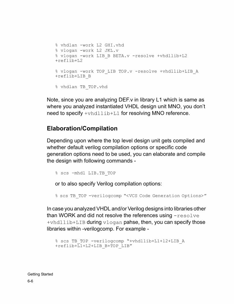
6-6
Getting Started
% vhdlan -work L2 GHI.vhd% vlogan -work L2 JKL.v% vlogan -work LIB_B BETA.v -resolve +vhdllib+L2 +reflib+L2
% vlogan -work TOP_LIB TOP.v -resolve +vhdllib+LIB_A +reflib+LIB_B
% vhdlan TB_TOP.vhd
Note, since you are analyzing DEF.v in library L1 which is same as where you analyzed instantiated VHDL design unit MNO, you don’t need to specify +vhdllib+L1 for resolving MNO reference.
Elaboration/Compilation
Depending upon where the top level design unit gets compiled and whether default verilog compilation options or specific code generation options need to be used, you can elaborate and compile the design with following commands -
% scs -mhdl LIB.TB_TOP
or to also specify Verilog compilation options:
% scs TB_TOP -verilogcomp “<VCS Code Generation Options>”
In case you analyzed VHDL and/or Verilog designs into libraries other than WORK and did not resolve the references using -resolve +vhdllib+LIB during vlogan pahse, then, you can specify those libraries within -verilogcomp. For example -
% scs TB_TOP -verilogcomp “+vhdllib+L1+l2+LIB_A +reflib+L1+L2+LIB_B+TOP_LIB”
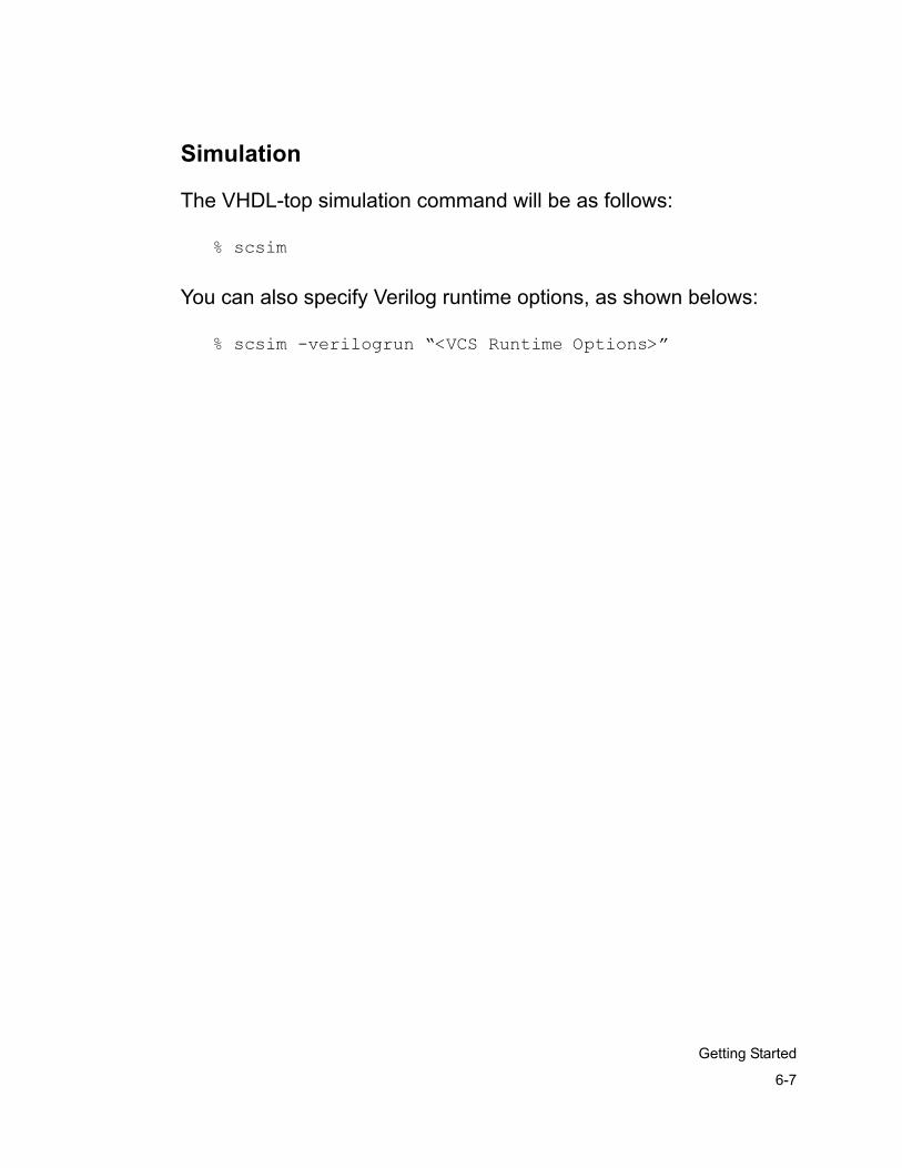
6-7
Getting Started
Simulation
The VHDL-top simulation command will be as follows:
% scsim
You can also specify Verilog runtime options, as shown belows:
% scsim -verilogrun “<VCS Runtime Options>”

6-8
Getting Started
Verilog-Top Mixed Language Flow Example
The following example illustrates some basic command sequences used in a typical Verilog-top multi-layer mixed-HDL design. The source files can be complied in the “WORK” or other logical libraries. Resolving the VHDL references in the Verilog modules can be relaxed or enforced using different options.
Design Hierarchy
TB_TOP (Verilog) TOP (VHDL) ALPHA (VHDL) ABC (VHDL) DEF (Verilog) MNO (VHDL) BETA (Verilog) GHI (VHDL) JKL (Verilog)
TB_TOP (Verilog)
TOP (VHDL)
AUNIT (VHDL)
ABC (VHDL) DEF (Verilog)
MNO (VHDL)
BUNIT (Verilog)
GHI (VHDL) JKL (Verilog)
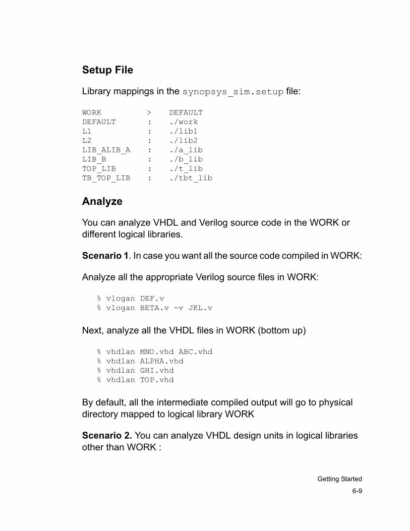
6-9
Getting Started
Setup File
Library mappings in the synopsys_sim.setup file:
WORK > DEFAULTDEFAULT : ./workL1 : ./lib1L2 : ./lib2LIB_ALIB_A : ./a_libLIB_B : ./b_libTOP_LIB : ./t_libTB_TOP_LIB : ./tbt_lib
Analyze
You can analyze VHDL and Verilog source code in the WORK or different logical libraries.
Scenario 1. In case you want all the source code compiled in WORK:
Analyze all the appropriate Verilog source files in WORK:
% vlogan DEF.v% vlogan BETA.v -v JKL.v
Next, analyze all the VHDL files in WORK (bottom up)
% vhdlan MNO.vhd ABC.vhd% vhdlan ALPHA.vhd% vhdlan GHI.vhd% vhdlan TOP.vhd
By default, all the intermediate compiled output will go to physical directory mapped to logical library WORK
Scenario 2. You can analyze VHDL design units in logical libraries other than WORK :
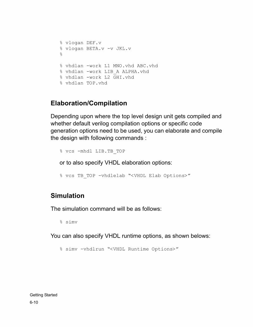
6-10
Getting Started
% vlogan DEF.v% vlogan BETA.v -v JKL.v%
% vhdlan -work L1 MNO.vhd ABC.vhd% vhdlan -work LIB_A ALPHA.vhd% vhdlan -work L2 GHI.vhd% vhdlan TOP.vhd
Elaboration/Compilation
Depending upon where the top level design unit gets compiled and whether default verilog compilation options or specific code generation options need to be used, you can elaborate and compile the design with following commands :
% vcs -mhdl LIB.TB_TOP
or to also specify VHDL elaboration options:
% vcs TB_TOP -vhdlelab “<VHDL Elab Options>”
Simulation
The simulation command will be as follows:
% simv
You can also specify VHDL runtime options, as shown belows:
% simv -vhdlrun “<VHDL Runtime Options>”
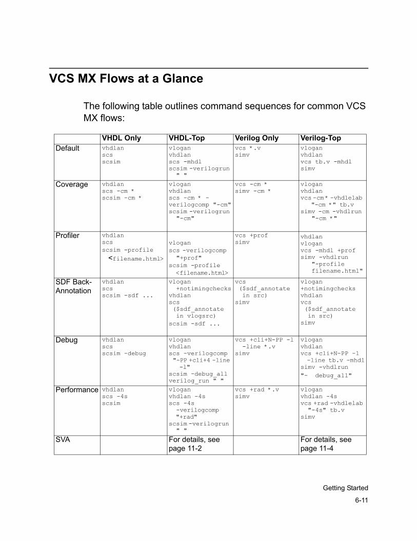
6-11
Getting Started
VCS MX Flows at a Glance
The following table outlines command sequences for common VCS MX flows:
VHDL Only VHDL-Top Verilog Only Verilog-TopDefault vhdlan
scsscsim
vloganvhdlanscs -mhdlscsim -verilogrun " "
vcs *.vsimv
vloganvhdlanvcs tb.v -mhdlsimv
Coverage vhdlanscs -cm *scsim -cm *
vloganvhdlanscs -cm * -verilogcomp "-cm"scsim -verilogrun "-cm"
vcs -cm *simv -cm *
vloganvhdlanvcs -cm * -vhdlelab
"-cm *" tb.vsimv -cm -vhdlrun
"-cm *"
Profiler vhdlanscs scsim -profile
<filename.html>
vloganscs -verilogcomp "+prof"
scsim -profile <filename.html>
vcs +profsimv
vhdlanvloganvcs -mhdl +profsimv -vhdlrun
"-profile filename.html"
SDF Back-Annotation
vhdlanscs scsim -sdf ...
vlogan +notimingchecks
vhdlanscs ($sdf_annotate in vlogsrc)
scsim -sdf ...
vcs ($sdf_annotate in src)
simv
vlogan +notimingchecksvhdlanvcs ($sdf_annotate in src)
simv
Debug vhdlanscs scsim -debug
vloganvhdlanscs -verilogcomp "-PP +cli+4 -line
-l"scsim -debug_all verilog_run " "
vcs +cli+N-PP -l -line *.vsimv
vloganvhdlanvcs +cli+N-PP -l -line tb.v -mhdlsimv -vhdlrun "- debug_all"
Performance vhdlanscs -4sscsim
vloganvhdlan -4sscs -4s -verilogcomp "+rad"
scsim -verilogrun " "
vcs +rad *.vsimv
vloganvhdlan -4svcs +rad -vhdlelab "-4s" tb.v
simv
SVA For details, see page 11-2
For details, see page 11-4
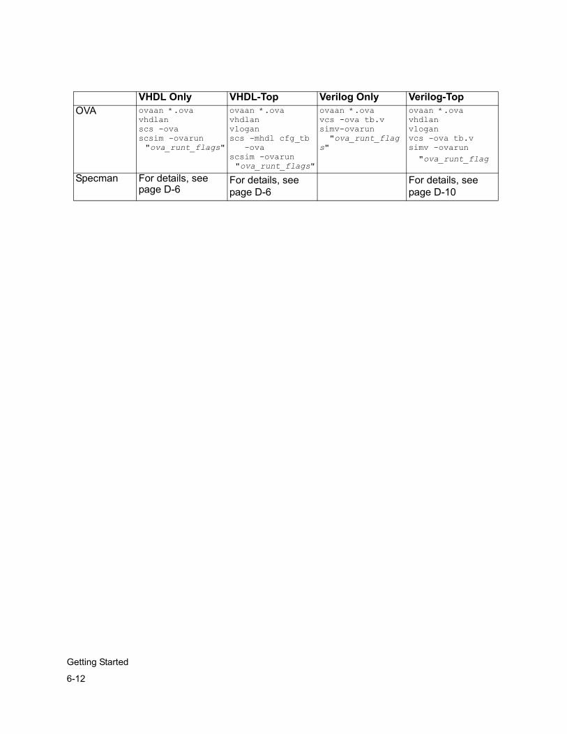
6-12
Getting Started
OVA ovaan *.ovavhdlanscs -ovascsim -ovarun "ova_runt_flags"
ovaan *.ovavhdlanvloganscs -mhdl cfg_tb -ovascsim -ovarun "ova_runt_flags"
ovaan *.ovavcs -ova tb.vsimv-ovarun "ova_runt_flag
s"
ovaan *.ovavhdlanvloganvcs -ova tb.vsimv -ovarun "ova_runt_flag
Specman For details, see page D-6
For details, see page D-6
For details, see page D-10
VHDL Only VHDL-Top Verilog Only Verilog-Top
7-1
Using scsim to Simulate Your Design
7Simulating Your Design 2
There are two basic methods you can use to simulate your MX design:
• If you analyzed and compiled your design as VHDL-only or VHDL-top, you will run a simulation using the scsim executable. For details on this process, see “Running and Controlling a Simulation Using the scsim Executable” on page 7-2.
• If you compiled your design as Verilog-only, or Verilog-top, you will run a simulation using the simv executable. For details on this process, see “Running and Controlling a Simulation Using the simv Executable” on page 7-41.
7-2
Using scsim to Simulate Your Design
Running and Controlling a Simulation Using the scsim Executable
This section explains how to run and control a simulation using the scsm executable from either the command line or the Graphical User Interface (GUI). The following topics are covered:
• Invoking a Simulation at the Command Line
• Invoking a Simulation From the VCS MX GUI
• Common scsim Simulation Options
• Using the VCS MX Control Lanaguage Commands
• Reading Simulation Profiler Results
• Invoking the Graphical User Interface
Invoking a Simulation at the Command Line
To invoke scsim, enter the following at the command line:
% scsim [options]
The options are one or more scsim options that enable you to control how VCS MX executes the simulation. For a complete list of scsim options, see the “To find the VHDL processes that are combined to create this function, cross-reference the combinational function name in the static elaboration report as we did earlier with the trigger function. section in this chapter.
7-3
Using scsim to SimulateYour Design
After entering scsim, a simulation prompt will appear at the command line. You control and monitor the simulation by entering VCS MX VHDL Command Language (SCL) commands at the simulation prompt (#). Detailed descriptions of these commands are available in the VCS MX Reference Guide.
Invoking a Simulation From the VCS MX GUI
To start the VCS MX GUI, type the following at the command line
% scirocco &
To invoke the simulator, do the following:
1. Click on Interactive menu button.
The Simulator Invocation Dialog window appears, as shown in the following figure.
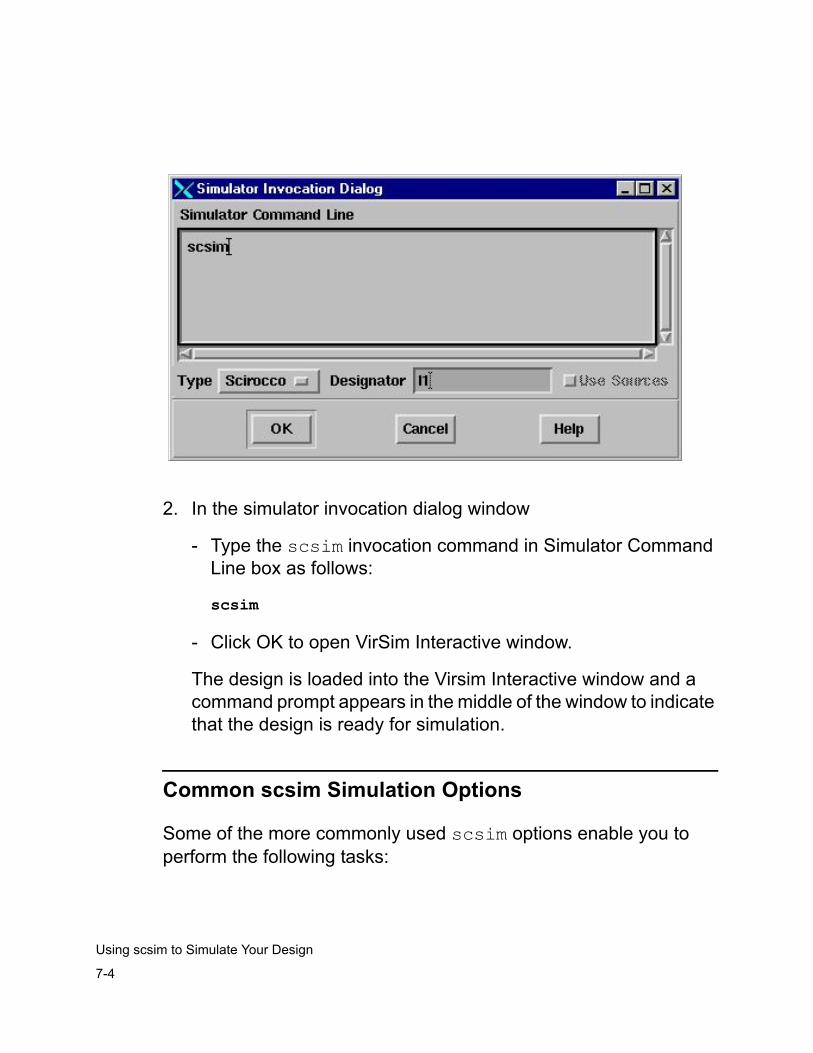
7-4
Using scsim to Simulate Your Design
2. In the simulator invocation dialog window
- Type the scsim invocation command in Simulator Command Line box as follows:
scsim
- Click OK to open VirSim Interactive window.
The design is loaded into the Virsim Interactive window and a command prompt appears in the middle of the window to indicate that the design is ready for simulation.
Common scsim Simulation Options
Some of the more commonly used scsim options enable you to perform the following tasks:
7-5
Using scsim to SimulateYour Design
• Simulate in functional VITAL mode
• Switch simulation to full debug mode
• Profile the simulation
• Simulate with SDF backannotation
• Queue simulation licenses
• Relax VHDL LRM conformance checking
Functional VITAL Simulation
When simulation your design in event mode, use -novitaltiming option to enable functional VITAL simulation mode. Using this option eliminates all timing-related aspects from the simulation of VITAL components. Timing-related aspects that are eliminated include Wire Delays, Path Delays, and Timing Checks. All outputs are assigned with 0-delay. The elimination of timing from the simulation of the VITAL components significantly improves performance of event simulations.
To enable functional VITAL for a scsim compiled for event simulation, type
% scsim -novitaltiming
For cycle mode simulations, VITAL components that are instantiated in the cycle partitions are automatically simulated using functional VITAL, there is no need to specify -novitaltiming option.
Note:Full-timing simulation of VITAL components cannot be performed using cycle mode simulation.
7-6
Using scsim to Simulate Your Design
Functional VITAL simulation applies to Level 1 compliant components. When using VITAL Level 0 compliant models, ensure that the coding style of the architecture closely follows that required for Level 1 compliant models in any of the timing areas (Wire Delay, Path Delay, and Timing Checks) that the model includes.
Because there are no rules and guidelines for the architecture's coding style in a Level 0 compliant model, VCS MX might not correctly ignore and only ignore the timing aspects of a Level 0 model. It is recommended that Level 0 architectures follow, as closely as possible, the style of Level 1 architectures to ensure that VCS MX correctly identifies the timing aspects of the model.
If you encounter problems in simulating Level 0 compliant VITAL models in functional VITAL or cycle mode, contact the Synopsys Technical Support Center for help on the coding style.
Note:Because all VITAL Level 1 compliant models are also Level 0 compliant, it is important to note that this guideline applies only to those models which are only Level 0 compliant and not Level 1 compliant.
Because functional VITAL discards all timing accuracy, this capability results in all SDF information being ignored. As a result, simulation results may not be correct if the simulation depends on timing accuracy.
7-7
Using scsim to SimulateYour Design
Switching a Simulation to Full Debug Mode
When you compile your design to run in compiled event mode, mixed event and cycle mode, or full cycle-based mode, you can switch running the simulation to full debug mode where source line stepping is enabled and you have full visibility to all design objects. This most useful when you run simulation and you hit a bug in the design that you decide to debug. You do not have to re-compile the design for debug mode, just use the -debug_all option. Using this option enables debug mode on the entire design, but simulation performance is greatly impacted.
If you want to enable debugging for only one or few design units but not the entire design, use the -debug_unit option. For example,
% scsim -debug_unit lib.ent_name
Profiling the Simulation
To generate the simulation profile report, use the -profile option on the scsim command line. For example,
% scsim -profile prof_out.html
The -profile option produces a formatted HTML report. This report is divided into four major sections that contain related information about the various phases of simulation, event simulation processes, cycle trigger and testbench functions, and cycle combinational processes. See “Reading Simulation Profiler Results” section for more information about how to read the profile.
See the “To find the VHDL processes that are combined to create this function, cross-reference the combinational function name in the static elaboration report as we did earlier with the trigger function.” section for more information about using this option.
7-8
Using scsim to Simulate Your Design
Simulating with SDF Backannotation
You can backannotate timing information from files in Standard Delay File (SDF) format into your design before simulation. SDF format is commonly used to communicate timing information among different simulators, synthesis tools, and layout tools.
To use SDF backannotation in VCS MX, use the -sdf option with scsim. The syntax to use SDF is
% scsim -sdf [min:|typ:|max:][region:] sdf_file]]
The SDF options allow you to indicate whether to use the minimum, typical, or maximum SDF values for backannotation. If you do not specify a value, VCS MX uses the typical timing values. The region indicates the portion of the design to backannotate using timing values from the sdf_file.
You can specify one or more SDF files to annotate the entire VHDL design or any portion of the hierarchy. For example, the following uses timing data from two different SDF files to annotate two different portions of a design:
% scsim -sdf /E/UUT/DESIGN1:myfile1.sdf \ -sdf max:/E/UUT/DESIGN2:myfile2.sdf
The above command
• Backannotates the VHDL design, starting from /E/UUT/DESIGN1, with typical timing values (the default) from the SDF file myfile1.sdf.
• Backannotates the VHDL design starting from /E/UUT/DESIGN2 with the maximum timing values from the SDF file myfile2.sdf.
7-9
Using scsim to SimulateYour Design
The following example shows how to use two SDF files to backannotate the same portion of a VHDL design:
% scsim -sdf min:/E/UUT/DESIGN:myfile1.sdf -sdf myfile2.sdf
The above command backannotates the VHDL design starting from /E/UUT/DESIGN using the minimum timing values from both myfile1.sdf and myfile2.sdf.
For information about using SDF version 3.0, see “SDF Version 3.0” in Appendix A of the VCS MX Reference Guide.
License Queueing
License queueing provides you with an effective way to make use of your purchased licenses. It is a much needed feature for situations such as mixedHDL and/or a simulation farm environment.
With license queueing, a "Ctrl-Z" or "Ctrl-C" will release the license immediately, enabling another job to check out the license instead of terminating. When resuming a job that is suspended by "Ctrl-Z," the job will re-acquire any available licenses or wait for the next available license (up until the timeout time specified). In addition, ^C and ^Z sent through VHPI is also supported by the license queueing feature. License queueing also works in cases where checkpoint/restore is used.

7-10
Using scsim to Simulate Your Design
With license queueing enabled, the job(s) can wait for the time specified by you in hours before timing out. This enables you to queue up more simultaneous jobs than your total number of licenses, and be confident that all the jobs will run. You will need to specify a timeout time long enough for all the jobs to run. This feature is extremely beneficial in the simulation farm environment. Also, mixedHDL simulation supports license queueing since both VCS and VCS MX have support for this feature.
Enabling License QueueingThere are two ways to enable the license queueing feature:
1. To enable license queueing for VCS MX at runtime, use with scsim the -licwait option along with a timeout time in hours, which will be the time the simulator will wait until finally giving up. The timeout time should be an integer greater than zero; any decimal part of the number will be ignored.
For example, to let the simulation job wait up to 4 hours before giving up, use
% scsim -licwait 4 -include cmd.input
7-11
Using scsim to SimulateYour Design
2. The second way to turn this feature on is to specify the LICENSE_WAIT_TIME variable in the synopsys_sim.setup file and assign it to the ultimate timeout time. If the variable is not present in the setup file, or if the variable is assigned an integer less than or equal to zero, license queueing will be off. Once again, any decimal places will be ignored. Below is the line you would add to the setup file to enable license queueing.
LICENSE_WAIT_TIME = 4
With the LICENSE_WAIT_TIME variable in the setup file set to an integer, you do not have to specify the -licwait option as a runtime option. However, if you do specify the -licwait option at runtime, this will override the setting in the setup file.
Relaxing VHDL LRM Conformance Checking
You can relax various VHDL Language Reference Manual (LRM) checks performed on your design. These checks include
• Integer to natural connections
To turn on relaxed checking to allow mapping ports of type integer to ports of type natural, use the scsim -xlrm option. It is to be noted that an illegal value could be passed from the integer to the natural number, resulting in a potential error in your simulation run.
• Driving a slice of a resolved composite signal
Use the scsim -xlrm to allow a process to drive just a slice or subset of a resolved composite signal. Simulation proceeds by creating drivers for the undriven subset and initializing them with the initial value of the subset of the corresponding target signal. Previously, an error was issued in this situation per the LRM.
7-12
Using scsim to Simulate Your Design
Using the VCS MX Control Lanaguage Commands
You can use basic VCS MX Control Language commands to perform the following tasks:
• Run the simulator
• Interrupt the simulator
• Restart the simulator
• Quit the simulator
You can also use more advanced programming constructs to control simulation flow. For information about using command procedures and programming with simulator commands, see “VCS MX Control Language” in Chapter 6 of the VCS MX Reference Guide.
The Unified Command-line Interface (UCLI) is for an interactive simulation or for a post-processing simulation using the UCLI interactive command language common to and consistent over multiple Synopsys verification technologies. We would encourage you to use UCLI as a default VCS MX control language for debugging, for interactive and post-processing simulations, and more. For more details on UCLI, see “Unified Command-line Interface” document available under VCS MX installation directory.
7-13
Using scsim to SimulateYour Design
Running the Simulator
When you run the simulator, you can specify the number of simulation timebase units you want the simulation to run. The simulation timebase unit is defined by
• The TIMEBASE variable value in the synopsys_sim.setup file.
• The value specified by the -t base_time option to the scs command.
To run the simulation for a specific amount of time, enter
# run time [timeunit]
If timeunit is not specified, the command runs the simulation for time (in simulation base_time units) and stops.
You can also run the simulation until the end of simulation time by entering either:
# run
Or
scsim -R
Interrupting the Simulator
Interrupting the simulator halts simulator execution immediately. You can interrupt the simulator by entering Control-c at the simulator prompt.
To interrupt the simulator from the simulator prompt, use the Control-c key sequence. The interrupt character Control-c is terminal-dependent.
7-14
Using scsim to Simulate Your Design
If you are running a compiled simulation, VCS MX displays the following prompt:
Interrupt detected in compiled code.Continue until next wait (y), or stop simulation immediately (n)? [y/n]:
Enter y to stop the simulation at the next wait statement. You can continue the simulation by entering the run command.
Enter n to stop the simulation immediately. VCS MX displays the following message:
You will not be able to rerun the simulation.Are you sure you want to stop immediately? [y/n]:
If you enter y, the simulation terminates and you cannot continue. To restart the simulation, use the VCS MX restart command, or quit the simulator and restart the simulator with scsim.
If you enter n, the simulation stops at the next wait statement. You can continue the simulation by entering the run command.
Restarting the Simulator
Restarting the simulator returns the simulation to time zero.
To restart the simulation from the simulator prompt, enter
# restart
7-15
Using scsim to SimulateYour Design
Quitting the Simulator
Quitting the simulator stops the simulation and returns you to the operating system. To quit the simulator from the simulator prompt, enter
# quit
Reading Simulation Profiler Results
VCS MX’s static profiler reports provide detailed information about cycle elaboration. In addition to the static reports, VCS MX can generate dynamic simulation profile reports.
The dynamic simulation profiler reports show you all the runtime statistics necessary to detect any simulation bottlenecks. The dynamic profiler reports list simulation time spent in each VHDL process as well as in each phase of simulation and points you to the line in the source code where the process is located. Additional information is provided for cycle regions, such as detailed listings of cycle optimized trigger functions and cycle optimized combinational functions along with the amount of simulation time spent in each.
The dynamic simulation profiler lets you make changes in your VHDL source code to yield the most improvement. The dynamic profile reports in conjunction with the static elaboration reports help to provide the maximum simulation performance with the least amount of effort.
See the “Profiling the Simulation” on page 2-7 for more information about how to generate the profile reports.
7-16
Using scsim to Simulate Your Design
The -profile option produces a formatted HTML report. This report is divided into four major sections that contain related information about the various phases of simulation, event simulation processes, cycle trigger and testbench functions, and cycle combinational processes.
The first two tables are always present in the report. The last two tables, related to cycle simulation, are only present if there are cycle regions simulated in the design.
Simulation Phases Table
The first table in the report lists summary information for major stages of the simulation executable. The following columns of information are shown:
• Simulation Phases
Shows the amount of time spent in each stage of compilation and simulation. The different phases are as follows:
- main programThe amount of time spent invoking the simulator executable.
- reading “.sim” filesThe amount of time spent in reading all the analysis information (.sim files).
- vhdl event elaborationThe amount of time the simulator spends performing elaboration of the event design regions.

7-17
Using scsim to SimulateYour Design
- vhdl cycle elaboration The amount of time the simulator spends performing elaboration of the cycle design regions. You need to perform this step only once. After elaboration is performed, you can reuse the object files created for multiple simulations.
- verilog compilationThe amount of time the simulator spends performing compilation of any verilog design regions.
- simulationThe total amount of time the simulator spends performing actual simulation of the design. The following regions all combine to form this total simulation time:
- vhdl signal network updateThe amount of time the simulator spends updating signal values in the design and propagating these values through the design interconnect. The time spent here is measured in real time only.
- monitor evaluationThe amount of time the simulator spends checking values and conditions for tracing, breakpoints, and monitors. It also includes the time for all VhPLI interactions. The time spent here is measured in real time only.
- vhdl debug evaluationThe amount of time spent simulating all design regions running in debuggable event mode. Any region simulating in this mode severely slows down the simulation performance. The time spent here is measured in real time only.
- vhdl event evaluationThe amount of time spent simulating all design regions running in compiled event mode. The time spent here is measured in real time only.
7-18
Using scsim to Simulate Your Design
- vhdl cycle evaluation The amount of time spent simulating all design regions running in cycle simulation mode. The time spent here is measured in real time only.
- vhdl event runtimeIt consists of all times in the event kernel other than process execution (event and debug), signal update and monitor evaluation. It’s the time spent in any SWIFT model or any time spent in cycle functions used to propogate event values through the cycle region for layered E-C-E (up & down the tree). The time spent here is measured in real time only.
- vhdl cycle runtime The small overhead cost of simulating in cycle mode. If the time spent in this stage of simulation exceeds that of the time spent in vhdl cycle evaluation, than the cycle regions are too small. The time spent here is measured in real time only.
- verilog evaluationThe amount of time spent simulating Verilog design regions in the design. The time spent here is measured in real time only.
- TOTALThe total time spent in the simulation executable. This is the time used to calculate all real time percentages in the profiler report.
• Real time
Shows the total elapsed time in seconds spent inside the simulation executable followed by the percentage of the total elapsed time spent in each phase of the simulator.
For simulation phases, VCS MX uses macro-measurement of the system clock to measure real time.
7-19
Using scsim to SimulateYour Design
These measurements are subject to quantization error for short or infrequent measurements.
Note:Real time is the measure of time of a UNIX process executed on a particular machine. You must be the only user of the machine to make accurate measurements.
• Delta cycle profile
Delta cycle activity is sampled to construct a histogram of the first nine delta cycles per timepoint. These histograms show whether a function is executed more than once per timepoint, which can be the result of feedback or reconvergent fanout.
A dot (.) means no activity in that delta cycle. An asterisk (*) means 100% of the simulation activity was spent in that delta cycle. The simulation activity in that delta cycle is reported as a number n, where n is between 0 and 9, and the simulation activity of that delta cycle is between n*10 to n*10+9 percent. For example, a value of 0 means between 0% to 9% of the simulation time was spent in that particular delta cycle, a value of 8 means between 80% and 89% percent of the simulation activity was spent in that particular delta cycle. The ninth delta cycle includes all activity for circuits with ten or more delta cycles.
......... no delta cycle activity occurred
.*....... all activity in the first delta cycle
.8..2.... 80-89% activity in the first delta cycle; 20-29% activity in the fourth delta cycle
Note that cycle regions collapse multiple event delta cycles into a single delta cycle.
7-20
Using scsim to Simulate Your Design
• Calls
Lists the number of times a function is called. Only available for the various simulation phases, and cycle-based trigger and combinational functions.
• User time
Time spent executing user code (seconds).
• System time
Time spent executing system code (seconds).
• User+Sys time
Sum of user time and system time. This time is independent of the system load and must be nominally equal to real time when the system is not loaded.
• Memory
Total memory (megabytes) allocated during a given simulation phase.
Event-based Processes Table
The second table in the dynamic profiler report lists information for event processes. The following columns of information are shown:
• Event-based Processes
Event-based processes are listed in the order of highest activity. The processes are named using the following syntax:
entity_name__architecture_name__process_name
7-21
Using scsim to SimulateYour Design
Only processes that take more than 0.1% of the total time are displayed.
• Real time
Shows the total elapsed time in seconds spent simulating the process followed by the percentage of the total elapsed time spent in each event process.
For event process activity and cycle trigger function and cycle combinatorial function activity, VCS MX uses micro-measurements of statistical sampling to measure real time.
These measurements are subject to quantization error for short or infrequent measurements.
Note:Real time is the measure of time of a UNIX process executed on a particular machine. You must be the only user of the machine to make accurate measurements.
• Delta cycle profile
Delta cycle activity is sampled to construct a histogram of the first nine delta cycles per timepoint. These histograms show whether the process is executed more than once per timepoint, which can be the result of feedback or reconvergent fanout.
7-22
Using scsim to Simulate Your Design
A dot (.) means no activity in that delta cycle. An asterisk (*) means 100% of the simulation activity was spent in that delta cycle. The simulation activity in that delta cycle is reported as a number n, where n is between 0 and 9, and the simulation activity of that delta cycle is between n*10 to n*10+9 percent. For example, a value of 0 means between 0% to 9% of the simulation time was spent in that particular delta cycle, a value of 8 means between 80% and 89% percent of the simulation activity was spent in that particular delta cycle. The ninth delta cycle includes all activity for circuits with ten or more delta cycles.
......... no delta cycle activity occurred
.*....... all activity in the first delta cycle
.8..2.... 80-89% activity in the first delta cycle; 20-29% activity in the fourth delta cycle
• Process type
Shows the simulation mode the process is running in, debug or event representing debuggable event simulation or compiled event simulation, respectively.
• Source file
Shows the name of the VHDL source file and the line in the file where the event process is located. For convenience, this field provides an HTML link to the file.
Cycle-based Trigger and Testbench Processes Table
The third table in the dynamic profiler report lists information about cycle simulation trigger and testbench functions. This table is present only if there are cycle regions being simulated in the design. The following columns of information are shown:
7-23
Using scsim to SimulateYour Design
• Cycle-based Trigger and Testbench Processes
Cycle simulation trigger and testbench functions are listed in the order of highest activity. The functions are named using the following syntax:
entity_name__architecture_name_tgf/tbf_ID
Only trigger and testbench functions that use more than 0.1% of the total time are displayed.
• Real time
Shows the total elapsed time in seconds spent simulating the function followed by the percentage of the total elapsed time spent in each function.
For event process activity and cycle trigger function and cycle combinatorial function activity, VCS MX-i uses micro-measurements of statistical sampling to measure real time.
These measurements are subject to quantization error for short or infrequent measurements.
Note:Real time is the measure of time of a UNIX process executed on a particular machine. You must be the only user of the machine to make accurate measurements.
• Delta cycle profile
Delta cycle activity is sampled to construct a histogram of the first nine delta cycles per timepoint. These histograms show whether the process is executed more than once per timepoint, which can be the result of feedback or reconvergent fanout.
7-24
Using scsim to Simulate Your Design
A dot (.) means no activity in that delta cycle. An asterisk (*) means 100% of the simulation activity was spent in that delta cycle. The simulation activity in that delta cycle is reported as a number n, where n is between 0 and 9, and the simulation activity of that delta cycle is between n*10 to n*10+9 percent. For example, a value of 0 means between 0% to 9% of the simulation time was spent in that particular delta cycle, a value of 8 means between 80% and 89% percent of the simulation activity was spent in that particular delta cycle. The ninth delta cycle includes all activity for circuits with ten or more delta cycles.
......... no delta cycle activity occurred
.*....... all activity in the first delta cycle
.8..2.... 80-89% activity in the first delta cycle; 20-29% activity in the fourth delta cycle
Note that cycle regions collapse multiple event delta cycles into a single delta cycle.
• Calls
Lists the number of calls made to the function during the simulation run.
• Size
Size of the executable code of the cycle function (number of instruction words). Generally, larger sized tgfs take longer to execute.
• Instructions per call
Average number of instructions executed per function call (ipc = real time * mips / calls). This metric is useful for measuring code improvements, however, quantization errors might result in inflated values.
7-25
Using scsim to SimulateYour Design
• Source processes
Number of sequential VHDL processes that are combined to create the specified cycle trigger or testbench function.
• Trigger Conditions
The conditions on which the trigger function is executed. For more information about trigger conditions and how to interpret the notation used, see “Static Cycle Elaboration Reports” on page 4-33.
Cycle-based Combinational Processes Table
The fourth table in the dynamic profiler report lists information about cycle simulation combinational functions. This table is present only if there are cycle regions being simulated in the design. The following columns of information are shown:
• Cycle-based Combinational Processes
Cycle simulation combinational functions are listed in the order of highest activity. See “Static Cycle Elaboration Reports” on page 4-33 for more information about cycle simulation combinational functions. The functions are named using the following syntax:
entity_name__architecture_name_cgf_ID
Only combinational functions that take more than 0.1% of the total time are displayed.
7-26
Using scsim to Simulate Your Design
• Real time
This total elapsed time in seconds spent simulating the function followed by the percentage of the total elapsed time spent in each function.
For event process activity and cycle trigger function and cycle combinatorial function activity, VCS MX VHDL uses micro-measurements of statistical sampling to measure real time.
These measurements are subject to quantization error for short or infrequent measurements.
Note:Real time is the measure of time of a UNIX process executed on a particular machine. You must be the only user of the machine to make accurate measurements.
• Delta cycle profile
Delta cycle activity is sampled to construct a histogram of the first nine delta cycles per timepoint. These histograms show whether the process is executed more than once per timepoint, which can be the result of feedback or reconvergent fanout.
A dot (.) means no activity in that delta cycle. An asterisk (*) means 100% of the simulation activity was spent in that delta cycle. The simulation activity in that delta cycle is reported as a number n, where n is between 0 and 9, and the simulation activity of that delta cycle is between n*10 to n*10+9 percent. For example, a value of 0 means between 0% to 9% of the simulation time was spent in that particular delta cycle, a value of 8 means between 80% and 89% percent of the simulation activity was spent in that particular delta cycle. The ninth delta cycle includes all activity for circuits with ten or more delta cycles.
7-27
Using scsim to SimulateYour Design
......... no delta cycle activity occurred
.*....... all activity in the first delta cycle
.8..2.... 80-89% activity in the first delta cycle; 20-29% activity in the fourth delta cycle
Note that cycle regions collapse multiple event delta cycles into a single delta cycle.
• Calls
Lists the number of calls made to the function during the simulation run.
• Size
Size of the executable code of the cycle function (number of instruction words). Generally, larger sized tgfs take longer to execute.
• Instructions per call
Average number of instructions executed per function call (ipc = real time * mips / calls). This metric is useful for measuring code improvements, however, quantization errors might result in inflated values.
• Source processes
Number of combinational VHDL processes that are combined to create the specified combinational function.
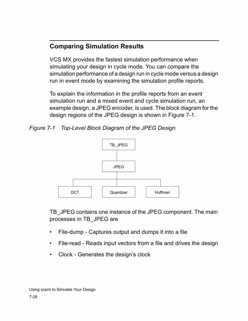
7-28
Using scsim to Simulate Your Design
Comparing Simulation Results
VCS MX provides the fastest simulation performance when simulating your design in cycle mode. You can compare the simulation performance of a design run in cycle mode versus a design run in event mode by examining the simulation profile reports.
To explain the information in the profile reports from an event simulation run and a mixed event and cycle simulation run, an example design, a JPEG encoder, is used. The block diagram for the design regions of the JPEG design is shown in Figure 7-1.
Figure 7-1 Top-Level Block Diagram of the JPEG Design
TB_JPEG contains one instance of the JPEG component. The main processes in TB_JPEG are
• File-dump - Captures output and dumps it into a file
• File-read - Reads input vectors from a file and drives the design
• Clock - Generates the design’s clock
TB_JPEG
JPEG
QuantizerDCT Huffman
7-29
Using scsim to SimulateYour Design
Event Mode Simulation Profile Report
To generate the runtime profile report for event mode simulation, use the following commands:
% scs TB_JPEG_CFG% scsim -profile profile_event.htm
The generated profile report is shown in Figure 7-2.
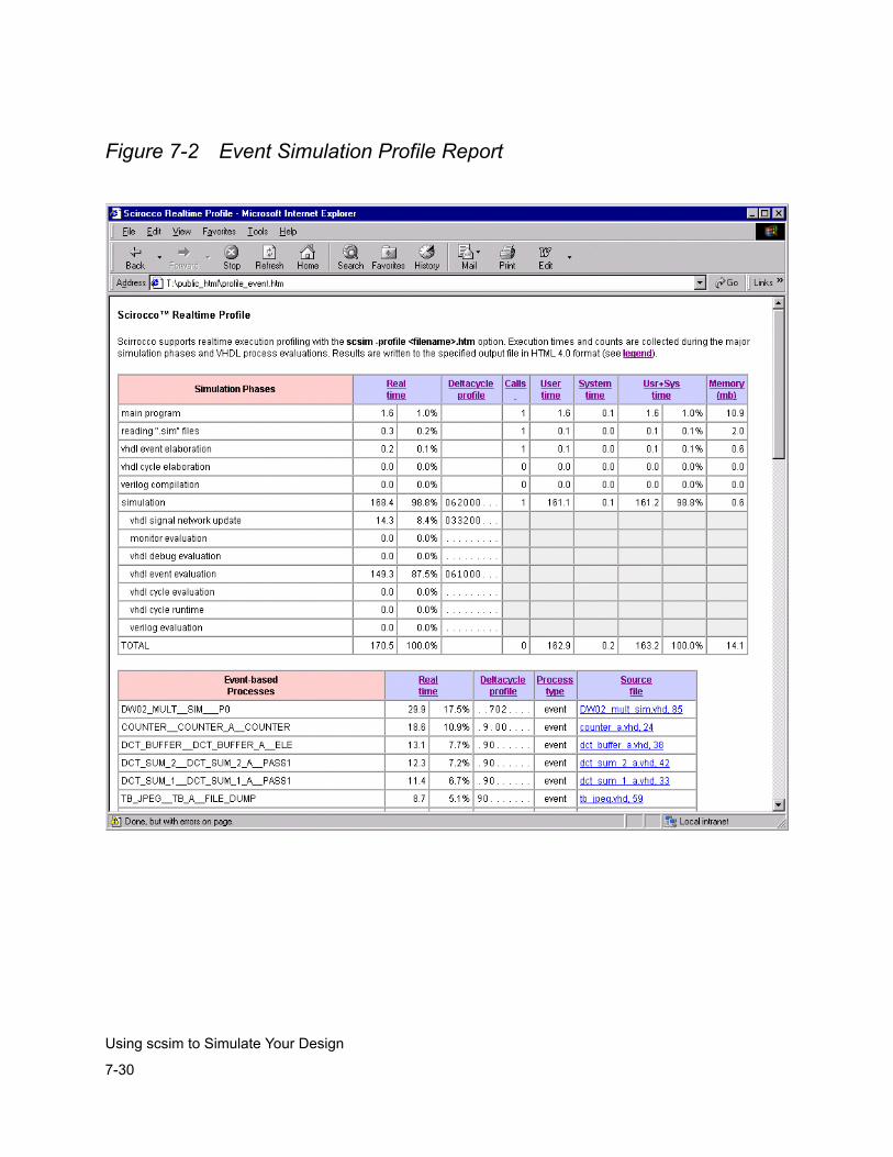
7-30
Using scsim to Simulate Your Design
Figure 7-2 Event Simulation Profile Report
7-31
Using scsim to SimulateYour Design
Reading Simulation Phases• TOTAL, the total time spent in the simulator, used 170.5 seconds
real time, and 163.2 seconds user+sys time. The real time and user+sys times are close, signifying a low machine load when the simulation was run. Whenever comparing the total times for two designs, use the total user+sys time as it does not vary based on machine load.
• simulation, the time spent actually running the design, used 168.4 seconds real time, or 98.8% of the TOTAL time spent in the executable. The total user+sys time was 161.2 seconds, or 98.8% of the total user+sys time.
• vhdl signal network update used 14.3 seconds real time or 8.4% of the TOTAL time.
• vhdl event evaluation used 149.3 seconds real time or 87.5% of the TOTAL time.
• vhdl cycle evaluation and vhdl cycle runtime used 0 seconds, which is correct since this is design was run in pure event mode.
Reading Event-based Processes
The processes are sorted from the most to the least amount of simulation time used.
• Process DW02_MULT__SIM__PO, starting at line 85 in the VHDL source file DWO2_mult_sim.vhd, ran for 29.9 seconds or 17.5% of the TOTAL time. This event process took the largest amount of simulation time.
• Process DCT_BUFFER__DCT_BUFFER_A_ELE, starting at line 38 in the VHDL source file dct_buffer_a.vhd, ran for 13.1 seconds or 7.7% of the TOTAL time.
7-32
Using scsim to Simulate Your Design
• Process TB_JPEG__TB_A__FILE_DUMP, starting at line 59 in the VHDL source file tb_jpeg.vhd, ran for 8.7 seconds or 5.1% of the TOTAL time.
• Process TB_JPEG__TB_A__FILE_READ, starting at line 108 in the VHDL source file tb_jpeg.vhd, ran for 1.9 seconds or 1.1% of the TOTAL time.
This information suggests that you examine the VHDL code for all processes running for a high percentage of the TOTAL time and if possible, try to improve the code for better simulation performance. See the VHDL Simulation Coding and Modeling Style Guide for more information about how to improve code for better simulation performance.
The Cycle-based Trigger and Testbench Processes and Cycle-based Combinational Processes tables are not present in the report as this design was run in pure event mode.
Mixed Event and Cycle Simulation Profile ReportFor mixed event and cycle mode simulation, the design has to be partitioned. Since the JPEG design is synthesizeable, the entire design can be accelerated by cycle optimizations and therefore is partitioned entirely into cycle. Only the testbench is run in event. The content of the partition file is
cycle -2state -perf JPEG_CFG
For more information about generating the partition file, see section “Creating a Partition File” on page 4-9.

7-33
Using scsim to SimulateYour Design
To elaborate the design and prepare for simulation, use the following command:
scs -partition part.file -perf_data static_elab.out TB_JPEG_CFG
To generate the runtime profile report for mixed event and cycle mode simulation, the following command is used:
scsim -profile profile_cycle.htm
The generated profile report is shown in Figure 7-3.
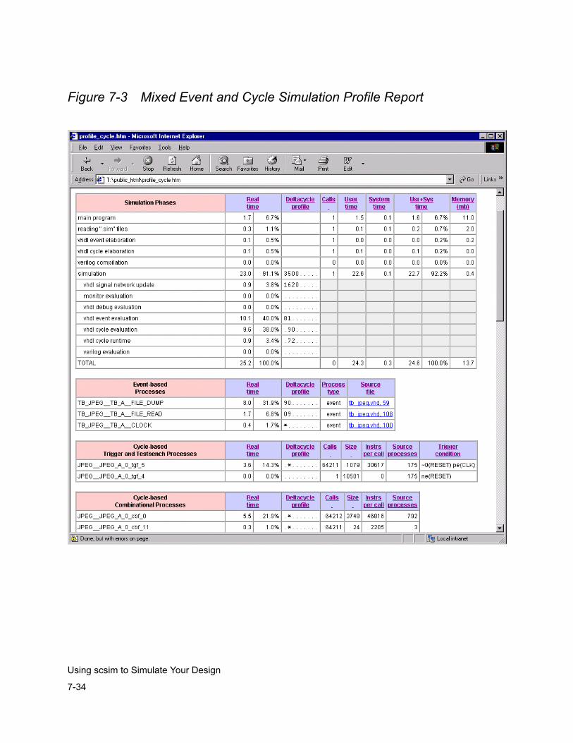
7-34
Using scsim to Simulate Your Design
Figure 7-3 Mixed Event and Cycle Simulation Profile Report
7-35
Using scsim to SimulateYour Design
Reading Simulation Phases• TOTAL used 25.2 seconds real time and 24.4 seconds user+sys
time.
• simulation used 23.0 seconds real time or 91.1% of the TOTAL time spent in the executable. The total user+sys time was 22.7 seconds, or 92.2% of the total user+sys time.
• vhdl signal network update used 0.9 seconds real time or 8.4% of the TOTAL time.
• vhdl event evaluation used 10.1 seconds real time or 40.0% of the TOTAL time.
• vhdl cycle evaluation used 9.6 seconds real time or 38.0% of the TOTAL time.
• vhdl cycle runtime used 0.9 seconds real time or 3.4% of the TOTAL time. This number is much smaller than the time spent in vhdl cycle evaluation indicating suitable cycle partitioning.
To find the gain in simulation performance from running mixed event-cycle mode over running pure event mode, compare the TOTAL user+sys times from each reports:
Event TOTAL / mixed TOTAL = speedup
163.2 / 24.6 = 6.6 X
Mixed event-cycle simulation is 6.6 times faster than event. In this example Real time values also provide similar numbers, but User+Sys time values are more accurate.
7-36
Using scsim to Simulate Your Design
Reading Event-based Processes
With the design partitioned, only the testbench processes are running in event mode. the other processes reported in the event simulation profile report are now being simulated in cycle mode.
• Process TB_JPEG__TB_A_FILE_DUMP, starting at line 59 in the VHDL source file tb_jpeg.vhd, ran for 8.0 seconds or 31.9% of the TOTAL time.
• Process TB_JPEG__TB_A_FILE_READ, starting at line 108 in the VHDL source file tb_jpeg.vhd, ran for 1.7 seconds or 6.8% of the TOTAL time.
Notice the total simulation times for each event process is similar between the pure event and the mixed event-cycle simulation run. However, since the mixed simulation runs so much faster, these processes now comprise a much larger percentage of the total simulation time (31.9% and 6.8% for mixed event-cycle simulation versus 5.1% and 1.1% respectively.)
Reading Cycle-based Trigger and Testbench Processes
The profile information for the cycle-based processes are reported in a different way from the event-based process. Cycle-based process information is reported with respect to the cycle trigger and testbench functions that are generated during cycle elaboration.
• Trigger function (tgf) JPEG__JPEG_A_0_tgf_5 runs for 3.6 seconds or 14.3% of the TOTAL time. This function controls the evaluation of 175 sequential processes in the design. This trigger function is called 64211 times during the simulation and executes 30617 machine instructions per call.
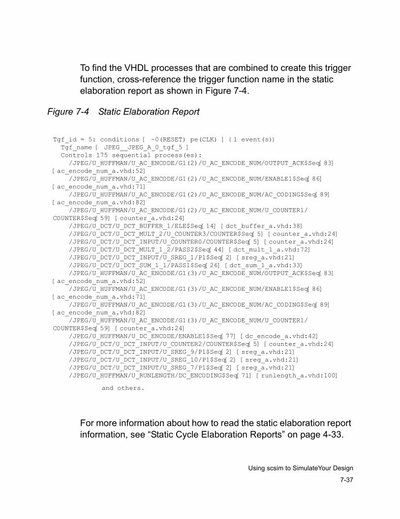
7-37
Using scsim to SimulateYour Design
To find the VHDL processes that are combined to create this trigger function, cross-reference the trigger function name in the static elaboration report as shown in Figure 7-4.
Figure 7-4 Static Elaboration Report
For more information about how to read the static elaboration report information, see “Static Cycle Elaboration Reports” on page 4-33.
Tgf_id = 5: conditions [ ~0(RESET) pe(CLK) ] {1 event(s)} Tgf_name [ JPEG__JPEG_A_0_tgf_5 ] Controls 175 sequential process(es): /JPEG/U_HUFFMAN/U_AC_ENCODE/G1(2)/U_AC_ENCODE_NUM/OUTPUT_ACK$Seq[83] [ac_encode_num_a.vhd:52] /JPEG/U_HUFFMAN/U_AC_ENCODE/G1(2)/U_AC_ENCODE_NUM/ENABLE1$Seq[86] [ac_encode_num_a.vhd:71] /JPEG/U_HUFFMAN/U_AC_ENCODE/G1(2)/U_AC_ENCODE_NUM/AC_CODING$Seq[89] [ac_encode_num_a.vhd:82] /JPEG/U_HUFFMAN/U_AC_ENCODE/G1(2)/U_AC_ENCODE_NUM/U_COUNTER1/COUNTER$Seq[59] [counter_a.vhd:24] /JPEG/U_DCT/U_DCT_BUFFER_1/ELE$Seq[14] [dct_buffer_a.vhd:38] /JPEG/U_DCT/U_DCT_MULT_2/U_COUNTER3/COUNTER$Seq[5] [counter_a.vhd:24] /JPEG/U_DCT/U_DCT_INPUT/U_COUNTER0/COUNTER$Seq[5] [counter_a.vhd:24] /JPEG/U_DCT/U_DCT_MULT_1_2/PASS2$Seq[44] [dct_mult_1_a.vhd:72] /JPEG/U_DCT/U_DCT_INPUT/U_SREG_1/P1$Seq[2] [sreg_a.vhd:21] /JPEG/U_DCT/U_DCT_SUM_1_1/PASS1$Seq[26] [dct_sum_1_a.vhd:33] /JPEG/U_HUFFMAN/U_AC_ENCODE/G1(3)/U_AC_ENCODE_NUM/OUTPUT_ACK$Seq[83] [ac_encode_num_a.vhd:52] /JPEG/U_HUFFMAN/U_AC_ENCODE/G1(3)/U_AC_ENCODE_NUM/ENABLE1$Seq[86] [ac_encode_num_a.vhd:71] /JPEG/U_HUFFMAN/U_AC_ENCODE/G1(3)/U_AC_ENCODE_NUM/AC_CODING$Seq[89] [ac_encode_num_a.vhd:82] /JPEG/U_HUFFMAN/U_AC_ENCODE/G1(3)/U_AC_ENCODE_NUM/U_COUNTER1/COUNTER$Seq[59] [counter_a.vhd:24] /JPEG/U_HUFFMAN/U_DC_ENCODE/ENABLE1$Seq[77] [dc_encode_a.vhd:42] /JPEG/U_DCT/U_DCT_INPUT/U_COUNTER2/COUNTER$Seq[5] [counter_a.vhd:24] /JPEG/U_DCT/U_DCT_INPUT/U_SREG_9/P1$Seq[2] [sreg_a.vhd:21] /JPEG/U_DCT/U_DCT_INPUT/U_SREG_10/P1$Seq[2] [sreg_a.vhd:21] /JPEG/U_DCT/U_DCT_INPUT/U_SREG_7/P1$Seq[2] [sreg_a.vhd:21] /JPEG/U_HUFFMAN/U_RUNLENGTH/DC_ENCODING$Seq[71] [runlength_a.vhd:100]
and others.
7-38
Using scsim to Simulate Your Design
Reading Cycle-based Combinational Process
Cycle-based Combinational Process information is reported with respect to the cycle combinational functions that are generated during cycle elaboration. For more information, see “Static Cycle Elaboration Reports” on page 4-33.
• Combinational function (cgf) JPEG__JPEG_A_0_cbf_0 runs for 5.5 seconds or 21.9% of the TOTAL time. This function controls the evaluation of 792 combinational logic processes in the design. This combinational function is called 64212 times during the simulation and executes 46816 machine instructions per call.
To find the VHDL processes that are combined to create this function, cross-reference the combinational function name in the static elaboration report as we did earlier with the trigger function.
Invoking the Graphical User Interface
VCS MX uses the DVE or VirSim Graphical User Interface. This GUI provides a complete suite of tools allowing you complete access to your design along with a project management tool to make simulation easier.
For more information on DVE, see "Discovery Visual Environment" Chapter 9,
The main elements of this graphical interface are as follows:
- Project Browser and Management Tool
- Interactive Window
- Hierarchy Browser
7-39
Using scsim to SimulateYour Design
- Waveform Window
- Source Window
- Register Window
The VirSim GUI lets you run simulations interactively or perform post processing of your simulation. For complete documentation of the VirSim GUI, see the VirSim Reference Manual.
Starting VirSim GUI for Interactive Simulation
To use the VCS MX GUI for interactive simulation, start the GUI with the command line options you want to pass to the simulator. For example,
% scirocco -nc -i cmd.in &
The command opens the Interactive text box. The scsim command and all the options you passed to VirSim appear in the Simulator Invocation Dialog.
Enter any other scsim options you want to use in the Simulator Command Line window and click on the OK button.
For more information about starting an interactive simulation, see the “Invoking the Interactive Window” section in the “Interactive Window” chapter of the VirSim Reference Manual.
Starting the VirSim GUI for Post-Processing
To use the VCS MX GUI for post-processing mode, start the GUI with -pp command line option.
% scirocco -pp &
7-40
Using scsim to Simulate Your Design
The command opens the Hierarchy window. From the pull-down menus, select File -> Open or press Ctrl-O. An Open File Dialog appears. From the Selection window, specify the name of the VCD+ file you want to load.
For more information about opening a file for post-processing, see “Opening and Closing History Files” section in the “Starting Virsim” chapter of the VirSim Reference Manual.
Starting the GUI with the Project Browser Window
To bring up the Project Browser window, start the GUI with -pb command line option.
% scirocco -pb &
The command opens the Project Browser window. For more information about using the Project Browser, see VirSim Reference Manual.
The scirocco Command
Syntaxscirocco [options]
Command Options
You can use all valid scsim options in the GUI Interactive Window. For example, to invoke interactive full debugging session, use
% scirocco -nc -debug_all &
Or it you want to invoke interactive session but debug few design units from the design, use
7-41
Using scsim to SimulateYour Design
% scirocco -nc -debug_unit \”unit1 unit2 unit2\” &
Note:For those command line options that require the arguments to be given in a quote (such as in the second example above), you need to proceed each quotation mark (“) with a backslash (\) while invoking scirocco.
Running and Controlling a Simulation Using the simv Executable
If you compiled your design as Verilog-only, or Verilog-top, then will run a simulation using the simv executable.
This chapter covers the following topics:
• Running a Mixed-HDL Simulation
• Common simv Runtime Options
• Common simv Tasks
• How VCS Prevents Time 0 Race Conditions
• Making a Verilog Model Protected and Portable
• Re-Invoking a Simulation With VirSim
• Using Interactive Commands
7-42
Using scsim to Simulate Your Design
Running a Mixed-HDL Simulation
You start simulating a mixed HDL design using the simv command line and VCS runtime options. However, you can also include two runtime options specific to mixed-HDL simulation:
-vhdlrun "VHDL command line options"For specifying scsim command line options that tell VCS MX how to simulate the VHDL part of the design.
+vcs+novhdldump For telling VCS MX not to record VHDL value changes in the VCD+ file for post-processing.
You can use the -vhdlrun runtime option on the simv command line.
The most commonly used options are as follows:
-debug_allSpecifies the slower simulating debugging mode.
-profile filename.htmlGenerates an HTML profile report, with the specified name, about how VCS MX simulates the VHDL part of the design.
The following is an example of using the -vhdlrun option:
simv -vhdlrun "-profile prof.html"
7-43
Using scsim to SimulateYour Design
Common simv Runtime Options
The runtime options discussed in this section are typically entered at the simv command line, but some of them can be compiled into the simv executable at compile-time.
Viewing the Compile-Time Options Used To Create The Executable-E program
Starts the program that displays the compile-time options that were on the vcs command line when you created the simv (or simv.exe) executable file. For example: simv -E echosimv -E echo > simvE.logYou cannot use any other runtime options with the -E option.
Simulating OpenVera Assertions
The following are runtime options for simulation OpenVEra Assertions:
-ova_quiet [1]Disables printing results on screen. The report file is not affected. With the 1 argument, only a summary is printed on screen.
-ova_report [filename]Generates a report file in addition to printing results on screen. Specifying the full path name of the report file overrides the default report name and location.
-ova_verboseAdds more information to the end of the report including assertions that never triggered and attempts that did not finish, and a summary with the number of assertions present, attempted, and failed.
7-44
Using scsim to Simulate Your Design
-ova_name name | pathnameSpecifies an alternative name or location and name for the ./simv.vdb/scov/results.db and ./simv.vdb/reports/ova.report files. You use this option if you want data and reports from a series of simulation runs. It is a way of keeping VCS MX from overwriting these files from a previous simulation. If you just specify a name the alternatively named files will be in the default directories. If you specify a pathname, with an argument containing the slash character /, you specify a different location and name for these files, for example:
-ova_name /net/design1/ova/run2
This example tells VCS MX to write run2.db and run2.report in the /net/design1/ova directory.
Runtime options for controlling how VCS MX writes its report on OpenVera Assertions. You can use them only if you compiled with the -ova_enable_diag compile-time option.
-ova_filterBlocks reporting of trivial if-then successes. These happen when an if-then construct registers a success only because the if portion is false (and so the then portion is not checked). With this option, reporting only shows successes in which the whole expression matched.
-ova_max_fail NLimits the number of failures for each assertion to N. When the limit is reached, the assertion is disabled. N must be supplied, otherwise no limit is set.
7-45
Using scsim to SimulateYour Design
-ova_max_success NLimits the total number of reported successes to N. N must be supplied, otherwise no limit is set. The monitoring of assertions continues, even after the limit is reached.
-ova_simend_max_fail NTerminates the simulation if the number of failures for any assertion reaches N. N must be supplied, otherwise no limit is set.
-ova_successEnables reporting of successful matches in addition to failures. The default is to report only failures.
Runtime options for functional coverage(enabled by the -ova_cov compile-time option):
-ova_covEnables functional coverage reporting.
-ova_cov_name filenameSpecifies the file name or the full path name of the functional coverage report file.
-ova_cov_db filenameSpecifies the path name of the initial coverage file. The initial coverage file is needed to set up the database.
CLI Command File Options-i filename
Specifies a file containing CLI commands that VCS MX executes when simulation starts. After VCS MX reaches the end of that file it takes commands from the standard input. Normally used along with the -s runtime option and a +cli+number compile-time option. A typical file for this option is the vcs.key file.
7-46
Using scsim to Simulate Your Design
-k filename | offSpecifies an alternative name or location for the vcs.key file into which VCS MX writes the CLI and VirSim interactive commands that you enter during simulation. The off argument tells VCS MX not to write this file.
+cliechoSpecifies that VCS MX display the CLI commands in a file that you specify with the -i option as VCS MX executes these CLI commands.
Stopping a Simulation-s
Stops simulation just as it begins, and enters interactive mode.Use with the +cli+number option.
Specifying VERA Object Files+vera_load=filename.vro
Specifies the VERA object file.
+vera_mload=filenameSpecifies a text file that contains a list of VERA object files.
Coverage Metrics Options-cm line|cond|fsm|tgl|obc|path
Specifies monitoring for the specified type or types of coverage. The arguments specifies the types of coverage:
lineMonitor for line or statement coverage.
condMonitor for condition coverage.
fsmMonitor for FSM coverage.
tglMonitor for toggle coverage.
7-47
Using scsim to SimulateYour Design
obcMonitor for observed coverage.
pathMonitor for path coverage.
If you want VCS MX to monitor for more than one type of coverage, use the plus (+) character as a delimiter between arguments, for example:
simv -cm line+cond+fsm+tgl+path
Don’t monitor for any other type of coverave when you monitor for observed coverage.
The -cm option is also a compile-time option and an option on the cmView command line.
-cm_dir directory_path_nameSpecifies and alternative name and location for the simv.cm directory. The -cm_dir option is also a compile-time option and a cmView command line option.
-cm_glitch periodSpecifies a glitch period during which VCS MX does not monitor for coverage caused by value changes. The period is an interval of simulation time specified with a non-negative integer.
-cm_log filenameAs a compile-time or runtime option, specifies a log file for monitoring for coverage during simulation. As a cmView command line option, specifies a log file for writing reports.
-cm_name filenameAs a compile-time or runtime option, specifies the name of the intermediate data files. On the cmView command line, specifies the name of the report files.
7-48
Using scsim to Simulate Your Design
-cm_tglfile filenameSpecifies displaying at runtime a total toggle count for one or more subhierarchies specified by the top-level module instance entered in the file. This option is also a compile-time option.
-cm_zipRequired when using the SWIFT interface to VMC models or SmartModels or when Undertow dumping is enabled.
Recording Where ACC Capabilities are Used+vcs+learn+pli
ACC capabilities enable debugging operations but they have a performance cost so you only want to enable them where you need them. This option keeps track of where you use them for debugging operations so that you can recompile your design and in the next simulation enable them only where you need them.When you use this option VCS MX writes the pli_learn.tab secondary PLI table file. You input this file when you recompile your design with the +applylearn compile-time option.
Suppressing the $stop System Task+vcs+ignorestop
Tells VCS MX to ignore the $stop system tasks in your source code.
Enabling and Disabling Specify Blocks+no_notifier
Suppresses the toggling of notifier registers that are optional arguments of system timing checks. The reporting of timing check violations is not affected. This is also a compile-time option.
+no_tchk_msgDisables the display of timing violations but does not disable the toggling of notifier registers in timing checks. This is also a compile-time option.
7-49
Using scsim to SimulateYour Design
+notimingcheckDisables timing check system tasks in your design. Using this option at runtime can improve the simulation performance of your design, depending on the number of timing checks that this option disables.You can also use this option at compile-time. Using this option at compile-time tells VCS MX to ignore timing checks when it compiles your design so the timing checks are not compiled into the executable and this results in a faster simulating executable than one that includes timing checks that are disabled by this option at runtime.If you need the delayed versions of the signals in negative timing checks but want faster performance, include this option at runtime. The delayed versions are not available if you use this option at compile-time. .VCS MX recognizes +notimingchecks to be the same as +notimingcheck when you enter it on the vcs or simv command line.
Specifying When Simulation Stops+vcs+stop+time
Stop simulation at the time value specified. The time value must be less than 232 or 4,294,967,296.
+vcs+finish+timeEnds simulation at the time value specified.The time value must be also less than 232.
For both of these options there is a special procedure for specifying time values larger than 232, see “Specifying A Very Long Time Before Stopping Simulation” on page 2-64.
7-50
Using scsim to Simulate Your Design
User-Defined Plusarg Options+plus-options
User-defined run-time options, which can be checked for by the $test$plusargs system task to perform some operation when the option is on the simv command line.
Recording Output-a filename
Specifies appending all messages from simulation to the bottom of the text in the specified file as well as displaying these messages in the standard output.
-l filenameSpecifies writing all messages from simulation to the specified file as well as displaying these messages in the standard output. Usage is letter "l" (lowercase "L") for log file.
Controlling Messages-q
Quiet mode. Suppress printing of VCS MX header and summary information.Suppresses proprietary message at beginningSuppresses VCS MX Simulation Report at the end (time, CPU time, data structure size, and date)
-VVerbose mode. Prints VCS MX version and extended summary information.Prints VCS MX compile and run-time version numbers, and copyright information, at start of simulation.
7-51
Using scsim to SimulateYour Design
+no_pulse_msgSuppresses pulse error messages, but not the generation of StE values at module path outputs when a pulse error condition occurs. You can enter this run-time option on the vcs command line.You cannot enter this option in the file you use with the -f compile-time option.
+sdfverboseBy default VCS MX displays no more than ten warning and ten error messages about back annotating delay information from SDF files. This option enables the display of all back annotation warning and error messages.This default limitation on back annotation messages applies only to messages displayed on the screen and written in the simulation log file. If you specify an SDF log file in the $sdf_annotate system task, this log file receives all messages.
+vcs+nostdoutDisables all text output from VCS MX including messages and text from $monitor and $display and other system tasks. VCS MX still writes this output to the log file if you include the -l option.
VCD+ Files
VCD+ files are simulation history files that VCS MX writes during simulation and DVE or VirSim reads after simulation to show you the simulation results. These are the runtime options that specify the size and contents of the VCD+. You specify these runtime options on the vcs command line.
7-52
Using scsim to Simulate Your Design
+vpdbufsize+number_of_megabytes To gain efficiency, VCD+ uses an internal buffer to store value changes before saving them on disk. This option modifies the size of that internal buffer. The minimum size allowed is what is required to share two value changes per signal. The default size is the size required to store 15 value changes for each signal but not less than 2 megabytes.
Note: The buffer size automatically is increased as needed to comply with the above limit.
+vpdfile+filenameSpecifies the name of the output VCD+ file (default is vcdplus.vpd). You must include the full file name with the .vpd extension.
+vpdfilesize +number_of_megabytesCreates a VCD+ file, which has a moving window in time while never exceeding a specified file size number_of_megabytes. When the VCD+ file size limit is reached, VCD+ will continue saving simulation history by overwriting older history. File size is a direct result of circuit size, circuit activity, and the data being saved. Test cases show that VCD+ file sizes will likely run from a few megabytes to a few hundred megabytes. Many users can share the same VCD+ history file, which may be a reason for saving all time value changes when you do simulation. You can save one history file for a design and overwrite it on each subsequent run.
7-53
Using scsim to SimulateYour Design
+vpdignoreTells VCS MX to ignore any $vcdplusxx system tasks and license checking. By default, VCS MX checks out a VCD+ PLI license if there is a $vcdplusxx system task in the Verilog source. In some cases, this statement is never executed and VCD+ PLI license checkout should be suppressed. The +vpdignore option performs the license suppression.
+vpddriversBy default, VCD+ records value changes only for the resolved value for each net. To also report value changes for all its drivers when there are more than one driver, use the +vdpdrivers option when simulating. The driver values, for example, enable the Logic Browser to identify which drivers produce an undesired X on the resolved net. This option affects performance and memory usage for larger designs or longer runs.
+vpdportsBy default, VCD+ does not store the port type for each signal, and the Hierarchy Browser views all signals as internal and not connected to a port. The +vpdports option causes VCD+ to store port information, which is then used by the Hierarchy Browser to show whether a signal is a port and if so its direction. This option to some extent affects simulation initialization time and memory usage for larger designs.
+vpdnocompressBy default, VCD+ compresses data as it is written to the VCD+ file. The user may disable this feature by supplying the +vpdnocompress command line option.
7-54
Using scsim to Simulate Your Design
+vpdnostrengthsBy default, VCD+ stores strength information on value changes to the VCD+ file. Use of this option may lead to slight improvements in simulator performance.
Controlling $gr_waves System Task Operations-grw filename
Sets the name of the $gr_waves output file to the specified filename.Default filename is grw.dump.
+vcs+grwavesoffSuppress $gr_waves system tasks.
VCD Files Options-vcd filename
Set name of $dumpvars output file to filename.The default filename is verilog.dump. A $dumpfile system task in the Verilog source code will override this option.
+vcs+dumpoff+t+htTurn off value change dumping ($dumpvars) at time t. ht is the high 32 bits of a time value greater than 32 bits.
+vcs+dumpon+t+htSuppress $dumpvars system task until time t. ht is the high 32 bits of a time value greater than 32 bits.
+vcs+dumpvarsoffSuppress $dumpvars system tasks.
7-55
Using scsim to SimulateYour Design
Specifying Min:Typ:Max Delays in Your Verilog Code and SDF Files+maxdelays
Specifies using the maximum delays in min:typ:max delay triplets in module path delays and timing check if you compiled your design with the +allmtm compile-time option. Also specifies using the maximum timing delays in min:typ:max delay triplets in an uncompiled SDF file. If you compiled the SDF file with the +allmtm compile-time option, the +maxdelays option specifies using the compiled SDF file with the maximum delays. Another use for this runtime option is to specify timing for SWIFT VMC and SmartModels and Synopsys hardware models when you also include the +override_model_delays runtime option.
+mindelaysSpecifies using the minimum delays in min:typ:max delay triplets in module path delays and timing check if you compiled your design with the +allmtm compile-time option. Also specifies using the minimum timing delays in min:typ:max delay triplets in an uncompiled SDF file. If you compiled the SDF file with the +allmtm compile-time option, the +mindelays option specifies using the compiled SDF file with the minimum delays. Another use for this runtime option is to specify timing for SWIFT VMC and SmartModels and Synopsys hardware models when you also include the +override_model_delays runtime option.
7-56
Using scsim to Simulate Your Design
+typdelaysSpecifies using the typical delays in min:typ:max delay triplets in module path delays and timing check if you compiled your design with the +allmtm compile-time option.Also specifies using the typical timing delays in min:typ:max delay triplets in an uncompiled SDF file. If you compiled the SDF file with the +allmtm compile-time option, the +typdelays option specifies using the compiled SDF file with the typical delays. This is a default option. By default VCS MX uses the typical delay in min:typ:max delay triplets your source code and in uncompiled SDF files (unless you specify otherwise with the mtm_spec argument to the $sdf_annotate system task,), and also by default VCS MX uses the compiled SDF file with typical values. Another use for this runtime option is to specify timing for SWIFT VMC and SmartModels and Synopsys hardware models when you also include the +override_model_delays runtime option.
Flushing Certain Output Text File Buffers
When VCS MX creates a log file, VCD file, or a text file specified with the $fopen system function, VCS MX writes the data for the file in a buffer and periodically dumps the data from the buffer to the file on disk. The frequency of these dumps varies depending on many factors including the amount of data that VCS MX has to write to the buffer as simulation or compilation progresses. If you need to see or use the latest information in these files more frequently than the rate at which VCS MX normally dumps this data, these options tell VCS MX to dump the data more frequently. How much more frequently also depends on many factors but the increased frequency will always be significant.
7-57
Using scsim to SimulateYour Design
+vcs+flush+log Increases the frequency of dumping both the compilation and simulation log files.
+vcs+flush+dumpIncreases the frequency of dumping all VCD files.
+vcs+flush+fopenIncreases the frequency of dumping all files opened by the $fopen system function
+vcs+flush+allIncreases the frequency of dumping all log files, VCD files, and all files opened by the $fopen system function
These options do not increase the frequency of dumping other text files including the VCDE files specified by the $dumpports system task or the simulation history file for LSI certification specified by the $lsi_dumpports system task.
These options can also be entered at compile-time. There is no particular advantage to entering them at compile-time.
Licensing Options+vcs+lic+vcsi
Checks out three VCSi licenses to run VCS.
+vcsi+lic+vcsChecks out three VCS licenses to run VCSi.
+vcs+lic+waitWait for network license if none is available when the job starts. Not supported on Windows.
7-58
Using scsim to Simulate Your Design
Enabling Overriding the Timing of a SWIFT SmartModel+override_model_delays
Enables the +mindelays, +typdelays, and +maxdelays runtime options to specify the timing used by SWIFT SmartModels instead of using the DelayRange parameter definition on the template file.
Option for the acc_handle_simulated_net PLI routine and MIPD annotation +vcs+mipd+noalias
For the PLI routine acc_handle_simulated_net, aliasing of a loconn net and a hiconn net across the port connection is disabled if MIPD delay annotation happens for the port. If you specify acc capability: mip or mipb in the pli.tab file, such aliasing is disabled only when actual MIPD annotation happens.
If during a simulation run, acc_handle_simulated_net is called before MIPD annotation happens, a warning message is issued. When this happens you can use this option to disable such aliasing for all ports whenever mip, mipb capabilities have been specified. This option works for reading an ASCII SDF file during simulation and not for compiled SDF files.
acc_handle_simulated_net is defined on IEEE Std 1364-1995 page 366.
Common simv Tasks
This section covers some of the common tasks you might want to perform using the simv executable. These tasks include the following:
• Saving and Restarting
• Saving and Restarting File I/O
7-59
Using scsim to SimulateYour Design
• Saving and Restarting with Runtime Options
• Restarting at The CLI Prompt
• Specifying A Very Long Time Before Stopping Simulation
• Passing Values From the Runtime Command Line
• Improving Performance
• Profiling the Simulation
Saving and Restarting
VCS MX provides a save and restart feature that allows checkpoints of the simulation to be saved at arbitrary times. The resulting checkpoint files can be executed at a later time, causing simulation to resume at the point immediately following the save.
Note: Save and restart is not supported on Windows.
Benefits of save and restart include:
• Regular checkpoints for interactively debugging problems found during long batch runs
• Use of plusargs to start action such as $dumpvars on restart
• Executes common simulation system tasks such as $reset just once in a regression
Restrictions of save and restart include:
• Requires extra Verilog code to manage the save and restart
• Must duplicate start-up code if handling plusargs on restart
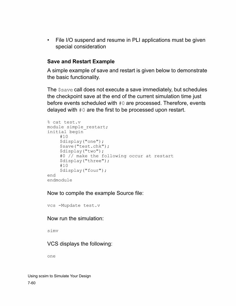
7-60
Using scsim to Simulate Your Design
• File I/O suspend and resume in PLI applications must be given special consideration
Save and Restart ExampleA simple example of save and restart is given below to demonstrate the basic functionality.
The $save call does not execute a save immediately, but schedules the checkpoint save at the end of the current simulation time just before events scheduled with #0 are processed. Therefore, events delayed with #0 are the first to be processed upon restart.
% cat test.vmodule simple_restart;initial begin
#10$display("one");$save("test.chk");$display("two");#0 // make the following occur at restart$display("three");#10$display("four");
endendmodule
Now to compile the example Source file:
vcs -Mupdate test.v
Now run the simulation:
simv
VCS displays the following:
one
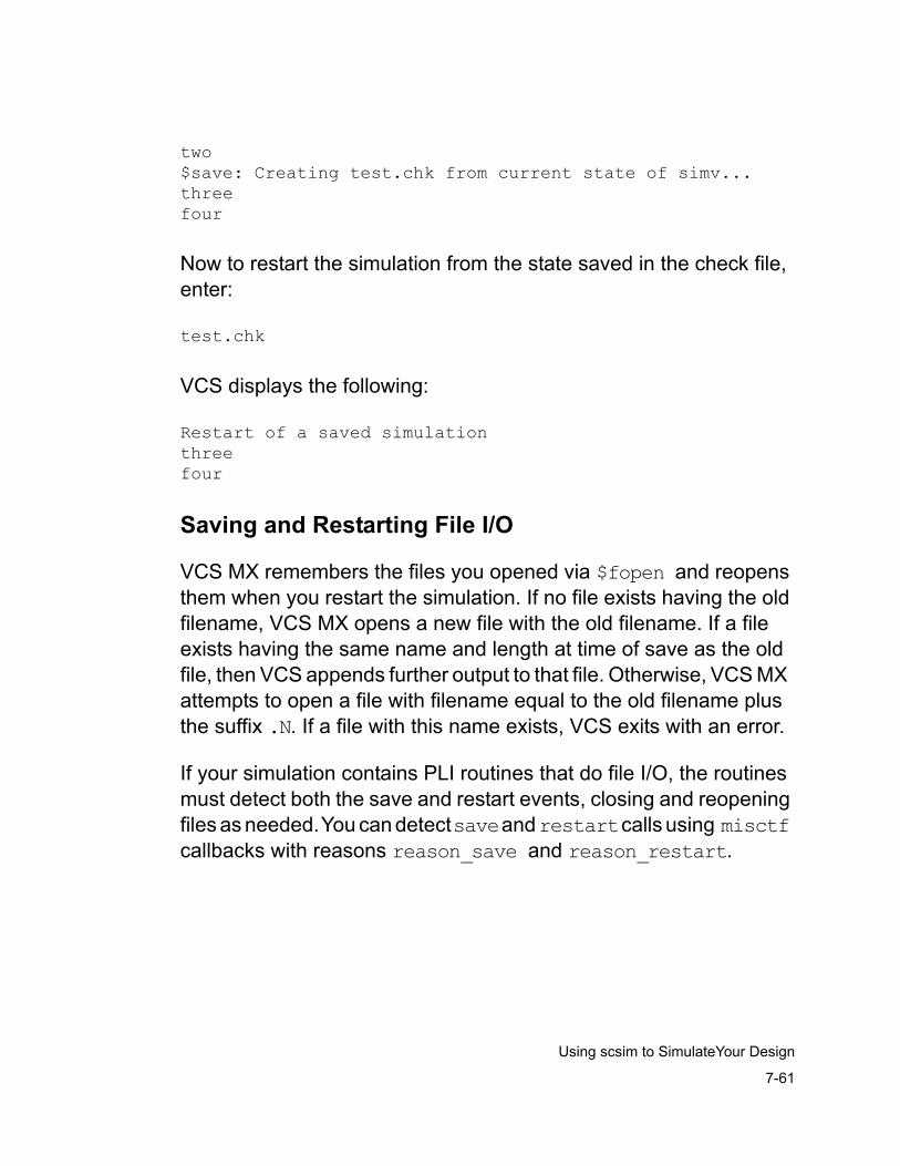
7-61
Using scsim to SimulateYour Design
two$save: Creating test.chk from current state of simv...threefour
Now to restart the simulation from the state saved in the check file, enter:
test.chk
VCS displays the following:
Restart of a saved simulationthreefour
Saving and Restarting File I/O
VCS MX remembers the files you opened via $fopen and reopens them when you restart the simulation. If no file exists having the old filename, VCS MX opens a new file with the old filename. If a file exists having the same name and length at time of save as the old file, then VCS appends further output to that file. Otherwise, VCS MX attempts to open a file with filename equal to the old filename plus the suffix .N. If a file with this name exists, VCS exits with an error.
If your simulation contains PLI routines that do file I/O, the routines must detect both the save and restart events, closing and reopening files as needed. You can detect save and restart calls using misctf callbacks with reasons reason_save and reason_restart.
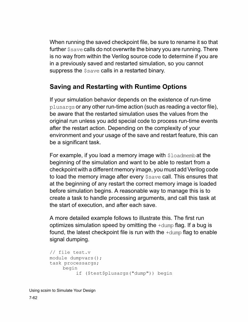
7-62
Using scsim to Simulate Your Design
When running the saved checkpoint file, be sure to rename it so that further $save calls do not overwrite the binary you are running. There is no way from within the Verilog source code to determine if you are in a previously saved and restarted simulation, so you cannot suppress the $save calls in a restarted binary.
Saving and Restarting with Runtime Options
If your simulation behavior depends on the existence of run-time plusargs or any other run-time action (such as reading a vector file), be aware that the restarted simulation uses the values from the original run unless you add special code to process run-time events after the restart action. Depending on the complexity of your environment and your usage of the save and restart feature, this can be a significant task.
For example, if you load a memory image with $loadmemb at the beginning of the simulation and want to be able to restart from a checkpoint with a different memory image, you must add Verilog code to load the memory image after every $save call. This ensures that at the beginning of any restart the correct memory image is loaded before simulation begins. A reasonable way to manage this is to create a task to handle processing arguments, and call this task at the start of execution, and after each save.
A more detailed example follows to illustrate this. The first run optimizes simulation speed by omitting the +dump flag. If a bug is found, the latest checkpoint file is run with the +dump flag to enable signal dumping.
// file test.vmodule dumpvars();task processargs;
beginif ($test$plusargs("dump")) begin
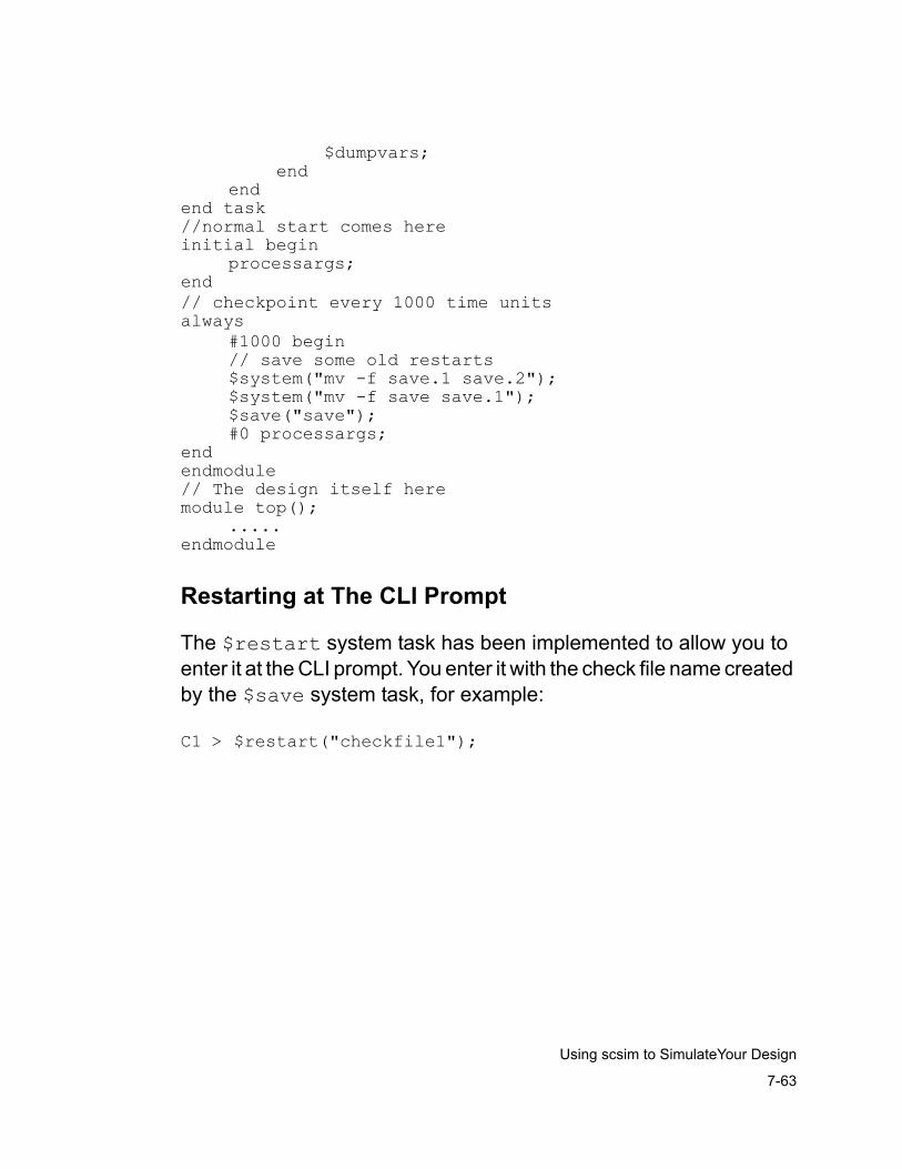
7-63
Using scsim to SimulateYour Design
$dumpvars;end
endend task//normal start comes hereinitial begin
processargs;end// checkpoint every 1000 time units always
#1000 begin// save some old restarts$system("mv -f save.1 save.2");$system("mv -f save save.1");$save("save");#0 processargs;
endendmodule// The design itself heremodule top();
.....endmodule
Restarting at The CLI Prompt
The $restart system task has been implemented to allow you to enter it at the CLI prompt. You enter it with the check file name created by the $save system task, for example:
C1 > $restart("checkfile1");
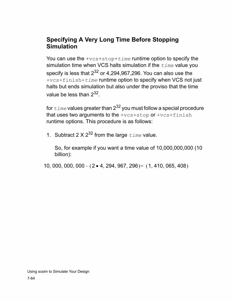
7-64
Using scsim to Simulate Your Design
Specifying A Very Long Time Before Stopping Simulation
You can use the +vcs+stop+time runtime option to specify the simulation time when VCS halts simulation if the time value you specify is less that 232 or 4,294,967,296. You can also use the +vcs+finish+time runtime option to specify when VCS not just halts but ends simulation but also under the proviso that the time value be less than 232.
for time values greater than 232 you must follow a special procedure that uses two arguments to the +vcs+stop or +vcs+finish runtime options. This procedure is as follows:
1. Subtract 2 X 232 from the large time value.
So, for example if you want a time value of 10,000,000,000 (10 billion):
10 000 000 000, , , 2 4 294 967 296, , ,•( ) 1 410 065 408, , ,( )=–
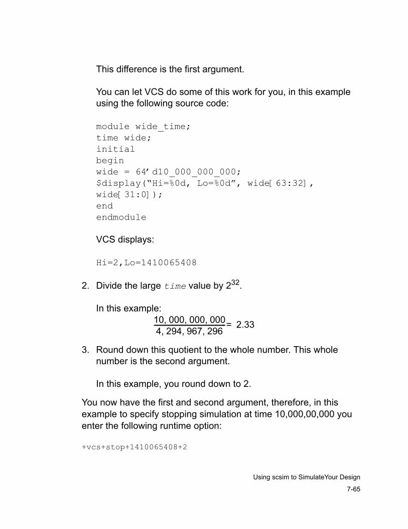
7-65
Using scsim to SimulateYour Design
This difference is the first argument.
You can let VCS do some of this work for you, in this example using the following source code:
module wide_time;time wide;initialbeginwide = 64’d10_000_000_000;$display(“Hi=%0d, Lo=%0d”, wide[63:32], wide[31:0]);endendmodule
VCS displays:
Hi=2,Lo=1410065408
2. Divide the large time value by 232.
In this example:
3. Round down this quotient to the whole number. This whole number is the second argument.
In this example, you round down to 2.
You now have the first and second argument, therefore, in this example to specify stopping simulation at time 10,000,00,000 you enter the following runtime option:
+vcs+stop+1410065408+2
10 000 000 000, , ,4 294 967 296, , ,---------------------------------------------- 2.33=
7-66
Using scsim to Simulate Your Design
Passing Values From the Runtime Command Line
The $value$plusargs system function can pass a value to a signal from the simv runtime command line using a +plusarg. The syntax is as follows:
integer = $value$plusargs("plusarg_format",signalname);
The plusarg_format argument specifies a user-defined runtime option for passing a value to the specified signal. It specifies the text of the option and the radix of the value that you pass to the signal.
The following code example contains this system function:
module valueplusargs;reg [31:0] r1;integer status;
initialbegin$monitor("r1=%0d at %0t",r1,$time);#1 r1=0;#1 status=$value$plusargs("r1=%d",r1);endendmodule
If you enter the following simv command line:
simv +r1=10
The $monitor system task displays the following:
r1=x at 0r1=0 at 1r1=10 at 2
7-67
Using scsim to SimulateYour Design
Improving Performance
When you simulate your design you can look for ways to improve the simulation performance. There are run-time options that enable VCS to simulate faster or slower. There is also a technique called profiling that tells you which modules in your design take the most CPU time.
Runtime Options that Accelerate or Impede Simulation
Some runtime options enable VCS to simulate your design faster because they allow VCS to skip certain operations. You should consider using these run-time options. These runtime options are as follows:
+vcs+dumpvarsoff Suppress $dumpvars system tasks.
+vcs+ignorestop Tells VCS to ignore the $stop system tasks in your source code.
+notimingcheck Disables timing check system tasks. Using this option at compile-time results in even faster simulation than using it at runtime.
The run-time options that specify writing to a file that slow down simulation. These run-time options are as follows:
-a filename All output of simulation is appended to filename as well as sent to the standard output.
-l filename All output of simulation is written to filename as well as to the standard output.
Other run-time options that specify operations other than the default operations also slow down simulation to some extent.
7-68
Using scsim to Simulate Your Design
Profiling the Simulation
If you include the +prof compile-time option when you compile your design, VCS MX generates the vcs.prof file during simulation. This file contains a profile of the simulation. It reports the following:
• The module instances in the hierarchy that use the most CPU time
• The module definitions whose instances use the most CPU time
• The Verilog constructs in those instances that use the most CPU time
You can use this information to see where in your design you might be able to modify your code for faster simulation performance.
The profile data in the vcs.prof file is organized into a number of “views” of the simulation. They are as follows:
• Top Level View
• Module View
• Instance View
• Module Construct Mapping View
• Top Level Construct View
• Construct View Across Design
Top Level ViewThis view shows you how much CPU time was used by:
• Any PLI application that executes along with VCS MX
• VCS MX for writing VCD and VCD+ files
7-69
Using scsim to SimulateYour Design
• VCS for internal operations that can’t be attributed to any part of your design
• The constructs and statements in your design.
The following is an example of the top level view:
=========================================================================== TOP LEVEL VIEW =========================================================================== TYPE %Totaltime--------------------------------------------------------------------------- PLI 0.00 VCD 0.00 KERNEL 29.06 DESIGN 70.94---------------------------------------------------------------------------
In this example there is no PLI application and VCS is not writing a VCD or VCD+ file. VCS used 70.94% of the CPU time to simulate the design, and 29.06% for internal operations, such as scheduling, that can’t be attributed to any part of the design. The designation KERNEL, is for these internal operations.
The designation VCD is for the simulation time used by the callback mechanisms inside VCS for writing either VCD or VCD+ files.
If there was CPU time used by a PLI application, you could use a tool such as gprof or Quantify to profile the PLI application.
Module ViewThis view shows you the module definitions whose instances use the most CPU time. Module definitions whose module instances collectively used less than 0.5% of the CPU time are not listed.
The following is an example of the module view:
=========================================================================== MODULE VIEW
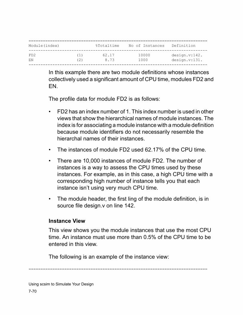
7-70
Using scsim to Simulate Your Design
===========================================================================Module(index) %Totaltime No of Instances Definition---------------------------------------------------------------------------FD2 (1) 62.17 10000 design.v:142.EN (2) 8.73 1000 design.v:131.---------------------------------------------------------------------------
In this example there are two module definitions whose instances collectively used a significant amount of CPU time, modules FD2 and EN.
The profile data for module FD2 is as follows:
• FD2 has an index number of 1. This index number is used in other views that show the hierarchical names of module instances. The index is for associating a module instance with a module definition because module identifiers do not necessarily resemble the hierarchal names of their instances.
• The instances of module FD2 used 62.17% of the CPU time.
• There are 10,000 instances of module FD2. The number of instances is a way to assess the CPU times used by these instances. For example, as in this case, a high CPU time with a corresponding high number of instance tells you that each instance isn’t using very much CPU time.
• The module header, the first ling of the module definition, is in source file design.v on line 142.
Instance ViewThis view shows you the module instances that use the most CPU time. An instance must use more than 0.5% of the CPU time to be entered in this view.
The following is an example of the instance view:
===========================================================================
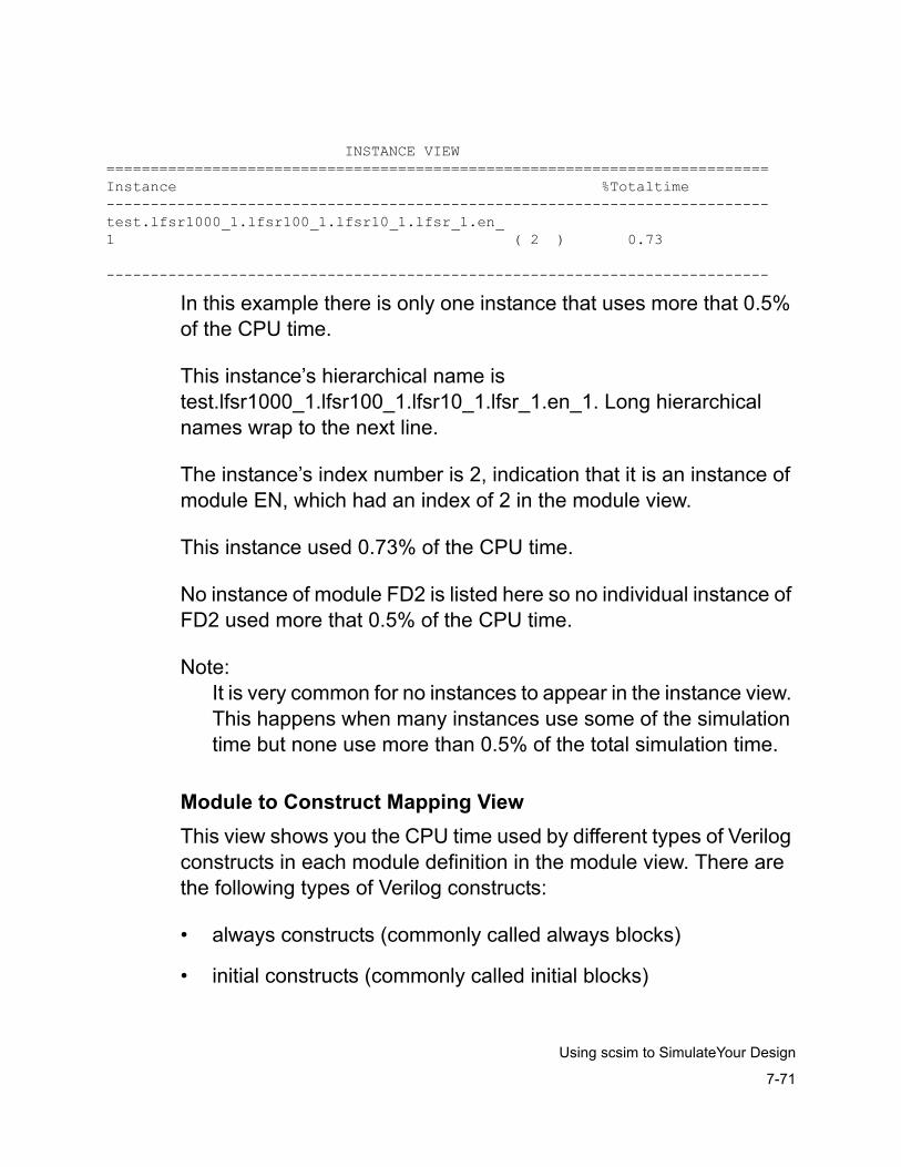
7-71
Using scsim to SimulateYour Design
INSTANCE VIEW===========================================================================Instance %Totaltime---------------------------------------------------------------------------test.lfsr1000_1.lfsr100_1.lfsr10_1.lfsr_1.en_1 ( 2 ) 0.73
---------------------------------------------------------------------------
In this example there is only one instance that uses more that 0.5% of the CPU time.
This instance’s hierarchical name is test.lfsr1000_1.lfsr100_1.lfsr10_1.lfsr_1.en_1. Long hierarchical names wrap to the next line.
The instance’s index number is 2, indication that it is an instance of module EN, which had an index of 2 in the module view.
This instance used 0.73% of the CPU time.
No instance of module FD2 is listed here so no individual instance of FD2 used more that 0.5% of the CPU time.
Note: It is very common for no instances to appear in the instance view. This happens when many instances use some of the simulation time but none use more than 0.5% of the total simulation time.
Module to Construct Mapping ViewThis view shows you the CPU time used by different types of Verilog constructs in each module definition in the module view. There are the following types of Verilog constructs:
• always constructs (commonly called always blocks)
• initial constructs (commonly called initial blocks)
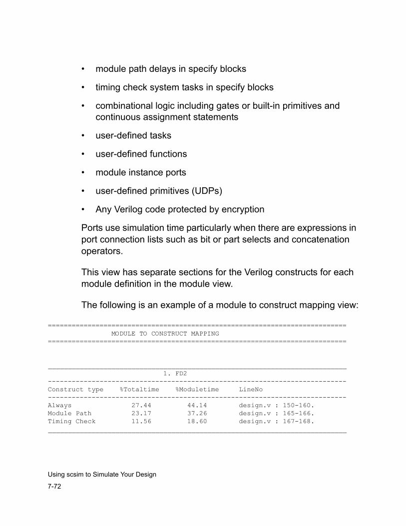
7-72
Using scsim to Simulate Your Design
• module path delays in specify blocks
• timing check system tasks in specify blocks
• combinational logic including gates or built-in primitives and continuous assignment statements
• user-defined tasks
• user-defined functions
• module instance ports
• user-defined primitives (UDPs)
• Any Verilog code protected by encryption
Ports use simulation time particularly when there are expressions in port connection lists such as bit or part selects and concatenation operators.
This view has separate sections for the Verilog constructs for each module definition in the module view.
The following is an example of a module to construct mapping view:
=========================================================================== MODULE TO CONSTRUCT MAPPING===========================================================================
___________________________________________________________________________ 1. FD2---------------------------------------------------------------------------Construct type %Totaltime %Moduletime LineNo---------------------------------------------------------------------------Always 27.44 44.14 design.v : 150-160.Module Path 23.17 37.26 design.v : 165-166.Timing Check 11.56 18.60 design.v : 167-168.___________________________________________________________________________
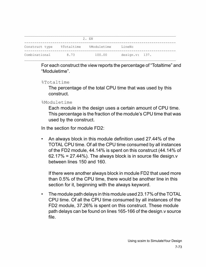
7-73
Using scsim to SimulateYour Design
___________________________________________________________________________ 2. EN---------------------------------------------------------------------------Construct type %Totaltime %Moduletime LineNo---------------------------------------------------------------------------Combinational 8.73 100.00 design.v: 137.___________________________________________________________________________
For each construct the view reports the percentage of “Totaltime” and “Moduletime”.
%TotaltimeThe percentage of the total CPU time that was used by this construct.
%ModuletimeEach module in the design uses a certain amount of CPU time. This percentage is the fraction of the module’s CPU time that was used by the construct.
In the section for module FD2:
• An always block in this module definition used 27.44% of the TOTAL CPU time. Of all the CPU time consumed by all instances of the FD2 module, 44.14% is spent on this construct (44.14% of 62.17% = 27.44%). The always block is in source file design.v between lines 150 and 160.
If there were another always block in module FD2 that used more than 0.5% of the CPU time, there would be another line in this section for it, beginning with the always keyword.
• The module path delays in this module used 23.17% of the TOTAL CPU time. Of all the CPU time consumed by all instances of the FD2 module, 37.26% is spent on this construct. These module path delays can be found on lines 165-166 of the design.v source file.
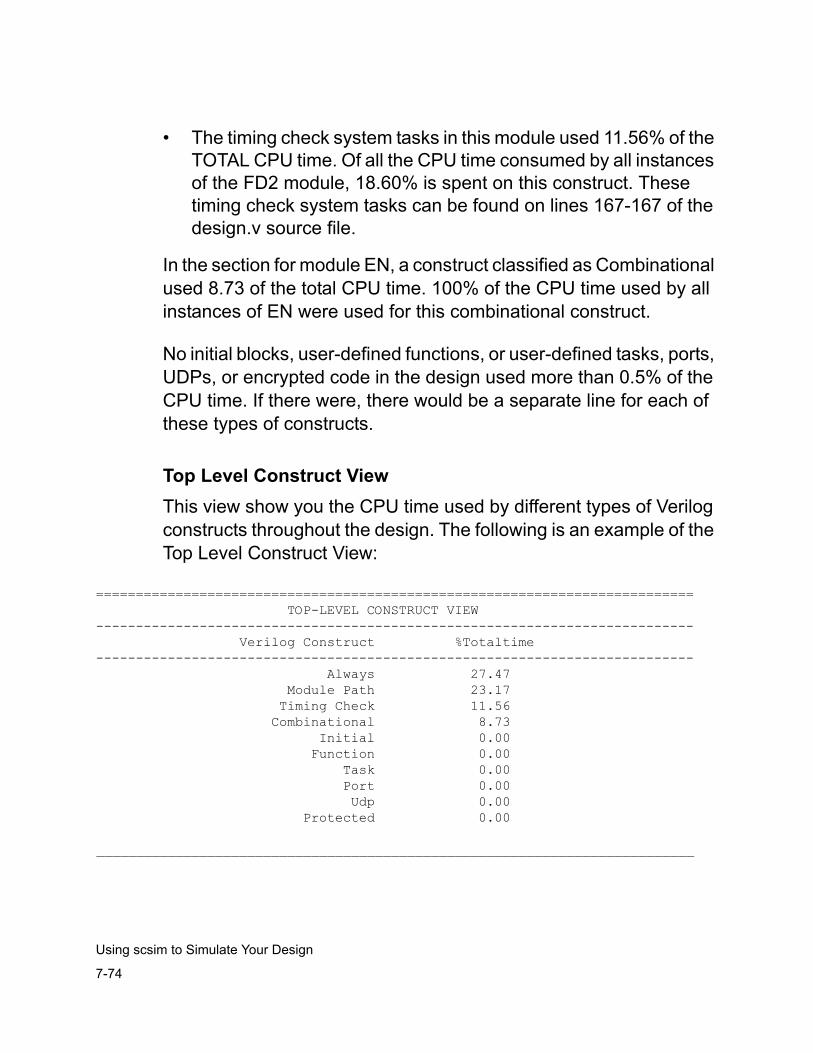
7-74
Using scsim to Simulate Your Design
• The timing check system tasks in this module used 11.56% of the TOTAL CPU time. Of all the CPU time consumed by all instances of the FD2 module, 18.60% is spent on this construct. These timing check system tasks can be found on lines 167-167 of the design.v source file.
In the section for module EN, a construct classified as Combinational used 8.73 of the total CPU time. 100% of the CPU time used by all instances of EN were used for this combinational construct.
No initial blocks, user-defined functions, or user-defined tasks, ports, UDPs, or encrypted code in the design used more than 0.5% of the CPU time. If there were, there would be a separate line for each of these types of constructs.
Top Level Construct ViewThis view show you the CPU time used by different types of Verilog constructs throughout the design. The following is an example of the Top Level Construct View:
=========================================================================== TOP-LEVEL CONSTRUCT VIEW--------------------------------------------------------------------------- Verilog Construct %Totaltime--------------------------------------------------------------------------- Always 27.47 Module Path 23.17 Timing Check 11.56 Combinational 8.73 Initial 0.00 Function 0.00 Task 0.00 Port 0.00 Udp 0.00 Protected 0.00
___________________________________________________________________________
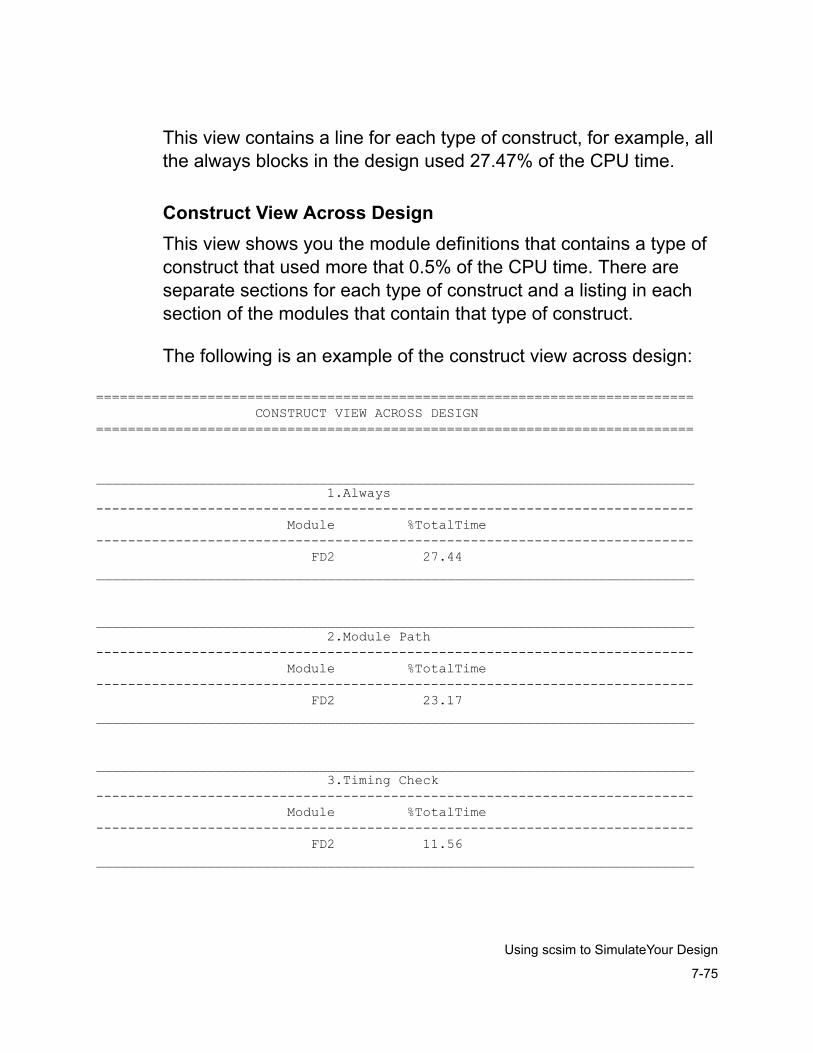
7-75
Using scsim to SimulateYour Design
This view contains a line for each type of construct, for example, all the always blocks in the design used 27.47% of the CPU time.
Construct View Across DesignThis view shows you the module definitions that contains a type of construct that used more that 0.5% of the CPU time. There are separate sections for each type of construct and a listing in each section of the modules that contain that type of construct.
The following is an example of the construct view across design:
=========================================================================== CONSTRUCT VIEW ACROSS DESIGN===========================================================================
___________________________________________________________________________ 1.Always--------------------------------------------------------------------------- Module %TotalTime--------------------------------------------------------------------------- FD2 27.44___________________________________________________________________________
___________________________________________________________________________ 2.Module Path--------------------------------------------------------------------------- Module %TotalTime--------------------------------------------------------------------------- FD2 23.17___________________________________________________________________________
___________________________________________________________________________ 3.Timing Check--------------------------------------------------------------------------- Module %TotalTime--------------------------------------------------------------------------- FD2 11.56___________________________________________________________________________
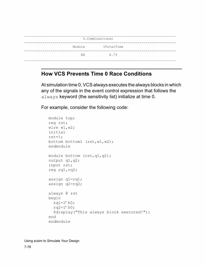
7-76
Using scsim to Simulate Your Design
___________________________________________________________________________ 4.Combinational--------------------------------------------------------------------------- Module %TotalTime--------------------------------------------------------------------------- EN 8.73___________________________________________________________________________
How VCS Prevents Time 0 Race Conditions
At simulation time 0, VCS always executes the always blocks in which any of the signals in the event control expression that follows the always keyword (the sensitivity list) initialize at time 0.
For example, consider the following code:
module top;reg rst;wire w1,w2;initialrst=1;bottom bottom1 (rst,w1,w2);endmodule
module bottom (rst,q1,q2);output q1,q2;input rst;reg rq1,rq2;
assign q1=rq1;assign q2=rq2;
always @ rstbegin rq1=1’b0; rq2=1’b0; $display("This always block executed!");endendmodule
7-77
Using scsim to SimulateYour Design
With other Verilog simulators there are two possibilities at time 0:
• The simulator executes initial block first, initializing reg rst, then the simulator evaluates the event control sensitivity list for the always block and executes the always block because rst initialized.
• The simulator evaluates the event control sensitivity list for the always block, and so far reg rst has not changed value during this time step so the simulator does not execute the always block, then the simulator executes the initial block and initializes rst. When this happens the simulator does not re-evaluate the event control sensitivity list for the always block.
Making a Verilog Model Protected and Portable
After a design is successfully verified using VCS, there is a separate tool available for those who want to make the design portable and protected. This tool, Verilog Model Compiler (VMC), enables you to secure your design and distribute it to your partners and internal or external customers without an NDA.
VMC is a model development tool used to generate portable models, starting with Verilog source and producing compiled SWIFT models. SWIFT is a language- and simulator-independent interface that allows your model to run with any SWIFT-compatible simulators; more than thirty simulators are now available.
VMC models contain no Verilog source code, so they are able to protect the intellectual property of the underlying design. This enables model developers to distribute their models without revealing the contents, because the models are secure. More importantly, the models are functionally exact because they are derived from the original Verilog description of the model
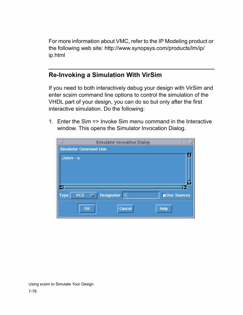
7-78
Using scsim to Simulate Your Design
For more information about VMC, refer to the IP Modeling product or the following web site: http://www.synopsys.com/products/lm/ip/ip.html
Re-Invoking a Simulation With VirSim
If you need to both interactively debug your design with VirSim and enter scsim command line options to control the simulation of the VHDL part of your design, you can do so but only after the first interactive simulation. Do the following:
1. Enter the Sim => Invoke Sim menu command in the Interactive window. This opens the Simulator Invocation Dialog.
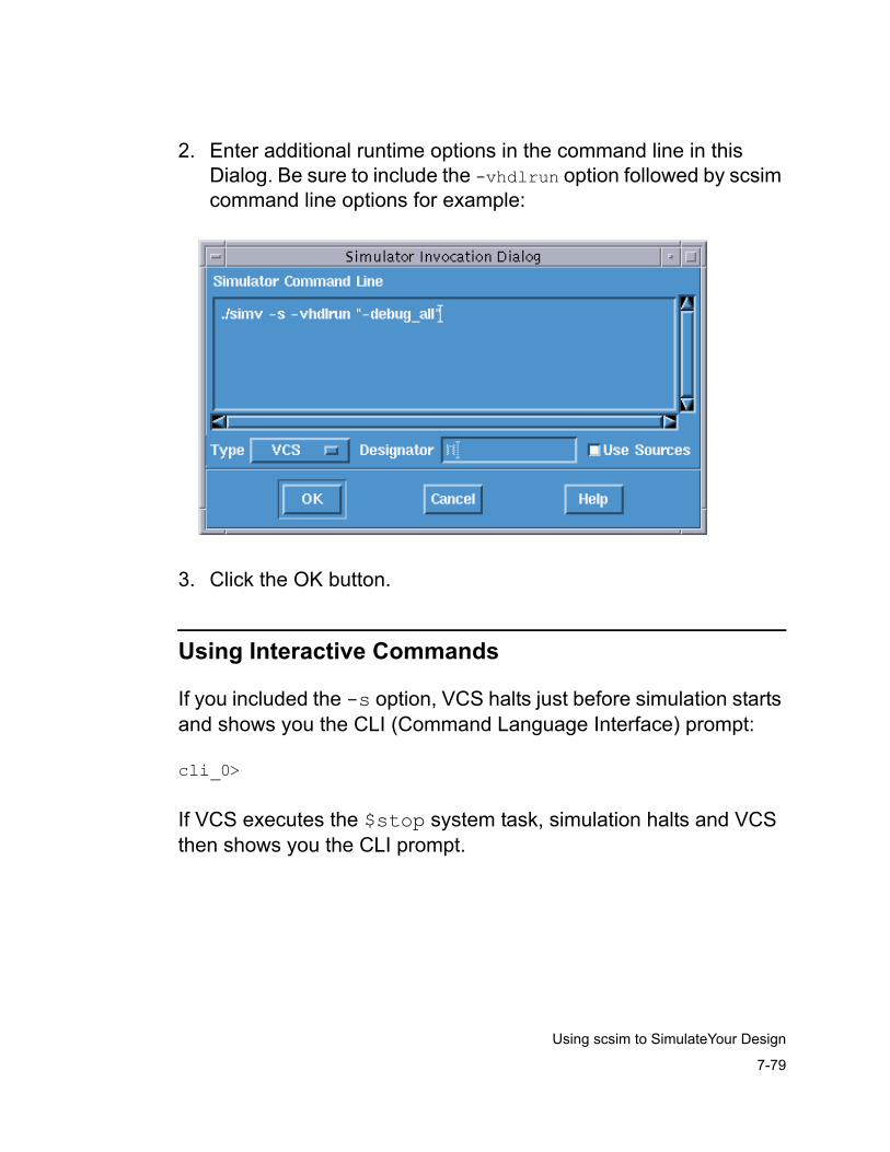
7-79
Using scsim to SimulateYour Design
2. Enter additional runtime options in the command line in this Dialog. Be sure to include the -vhdlrun option followed by scsim command line options for example:
3. Click the OK button.
Using Interactive Commands
If you included the -s option, VCS halts just before simulation starts and shows you the CLI (Command Language Interface) prompt:
cli_0>
If VCS executes the $stop system task, simulation halts and VCS then shows you the CLI prompt.
7-80
Using scsim to Simulate Your Design
This prompt is for entering CLI debugging commands. These commands allow you to display the values of signals in the current scope in the hierarchy, change scope, assign values to signals, apply breakpoints, and other debugging commands. These commands are described in the VCS User’s Guide.
You can enter CLI commands for both the Verilog and VHDL parts of your design.
The “Command” field in the VirSim Interactive window is also a prompt for CLI commands. Button commands in the “User Defined Buttons” area of the Interactive window are really CLI commands entered by VirSim.
If you are using VirSim to interactively debug your design, you can enter CLI commands for both the Verilog and VHDL parts of your design.
Special Rules For Interactive Commands
For mixed HDL simulation there are these special rules to keep in mind when entering interactive commands:
• When entering CLI commands to perform and operation on a signal or to specify a part of the hierarchy, in both the VHDL and Verilog part of a design, always use the “.” period character as the delimiter between instance names and before the signal name in hierarchical names.
• When entering commands for VHDL signals, part selects or slices are not supported.
• Commands that display drivers or loads do not do so across the VHDL/Verilog boundary of a mixed HDL design.
7-81
Using scsim to SimulateYour Design
• The oformat CLI command can specify 13 formats (%b|c|t|f|e|g|d|h|x|m|o|s|v), however only the binary (b)octal (o), hexadecimal (h or x) are valid in the VHDL part of the design, so if you set a format that is not b, o, h, or x, VCS displays a warning message and the previous format is retained for displaying VHDL values.
CLI Changes Caused By The TCL Shell Environment
A TCL shell environment enables you to use the both the VCS CLI and the VCS MX Command Language in both the VCS flow and VCS MX flow for mixed HDL simulation. This TCL shell environment, however has required a number of changes to the VCS CLI for mixed HDL simulation.
TCL treats the following as special characters: ’ ‘ " $ space, newline, and tab. To prevent TCL from attaching special meaning to these characters, enclose commands and arguments that contain them in curly braces { }. This section describes some of the instances when you should use these braces.
If you enter the scope CLI command to change scope to a Verilog instance names with an escaped identifier, you must enclose the escaped identifier with curly braces, and include the blank space that terminates the escaped identifier name inside the curly braces, for example:
scope {\_scope1.scope2 }
There is a different syntax for entering system tasks at the CLI prompt, you can’t simply enter the system task, but must include the system task as an argument, enclosed in curly braces, to the new call command. The syntax is as follows:
7-82
Using scsim to Simulate Your Design
call { $system_task(arg1,arg2,...)}
For example:
call { $vcdpluson(0,vlogdes1)}
Be sure to leave out the semicolon (;) at the end of the system task.
IMPORTANT: You can only enter system tasks when your current scope is in the Verilog part of the design.
The tick character ’ that is used for specifying a radix in some Verilog values, should be enclosed in curly braces, for example:
assign reg1 = {4’hf}
TCL also interprets certain CLI commands differently and therefore these commands are renamed.The renamed commands and their new names are as follows:
• The set command, for assigning values to a signal, is now the assign command.
• The info command, for displaying time and scope information, is now the vinfo command.
• The continue command, for resuming simulation, is now the vcontinue command.
Switching Command Languages
In mixed HDL simulation, VCS MX understands both the VCS Command Language Interface (CLI) and the VCS MX Control Language so during simulation you can switch from one to the other and back again. The command to make this switch and its options are as follows:
7-83
Using scsim to SimulateYour Design
changemode [-query | -verilog | -vhdl]
The -query option clarifies whether you currently have enabled the VCS MX Control Language or the VCS CLI.
The -verilog option specifies switching to the VCS CLI.
The -vhdl option species switching to the VCS MX Control Language.
Entering the changemode command without options toggles the command language from the current one to the other one.
If you switch to the VCS MX Control Language the special rules described above for interactive commands also hold true for VHDL part selects, or slices, and displaying drivers and loads across the VHDL/Verilog boundary. With the VCS MX Control Language use the “/” slash character as the delimiter in hierarchical names.
Note: If you are running VirSim for interactive debugging, you cannot enter the changemode command. The changemode command is for the text based interface for the VCS MX Command Language and the VCS CLI.
Hierarchical Name Syntax
Hierarchical name syntax in both the VCS MX Control Language and the VCS CLI is different depending on whether VHDL or Verilog is on top of the design hierarchy of a mixed HDL design.
7-84
Using scsim to Simulate Your Design
Here in the VCS flow, where Verilog is at the top of the hierarchy:
Hierarchical names do not begin with the delimiter.In The VCS MX Control Language a hierarchical name could be: top/U1/T1In the VCS CLI a hierarchical name could be: top.U1.T1
In the mixed HDL flow, where VHDL is at the top of the hierarchy:
Hierarchical names begin with the delimiter.In The VCS MX Control Language a hierarchical name could be: /top/U1/T1In the VCS CLI a hierarchical name could be: .top.U1.T1
8-1
Debugging and Post-Processing
8Debugging and Post-Processing 3
This chapter covers the following debugging and post-processing topics:
• Interactive Debugging Using the Command Line
• Interactive Simulation using the GUI
• Post-Processing for VHDL-Only and VHDL-Top Flows
• Post-Processing for Verilog-Only and Verilog-Top Flows
• VCS MX VHDL Timebase and Time Precision Resolution
• Comparing VCS CLI and VCS MX VHDL SCL Commands
8-2
Debugging and Post-Processing
Interactive Debugging Using the Command Line
When a VHDL-only or VHDL-top simulation starts, you are at the VCS MX command line prompt “#”. You can use almost all the VCS MX control langauge (SCL) commands used for pure VHDL simulation in mixed language simulation.
When entering commands to perform an operation on a signal or to specify a part of the hierarchy, in both the VHDL signal and Verilog part of a design, always use the / slash character as the delimiter between instance names and before the signal name in hierarchical names.
For more information about VCS MX control language, see “VCS MX Control Language” in Chapter 6 of the VCS MX Reference Guide.
Changing Between Command Languages
In mixed HDL simulation, you can use both the VCS Command Language Interface (CLI) and the VCS MX Control Language. This capability lets you change from one command interface to the other and back again during simulation.
You use the changemode command and its options to go back and forth between the interfaces. The command syntax and its options are as follows:
changemode [-query | -verilog | -vhdl]
-query
Displays the currently enable interface.
8-3
Debugging and Post-Processing
-verilog
Enables the VCS CLI.
-vhdl
Enables the VCS MX Control Language.
Using the changemode command without options toggles the command language from the current one to the other one.
If you change to CLI, the special rules described above for interactive commands also hold true for VHDL part selects, or slices, and displaying drivers and loads across the VHDL/Verilog boundary. With CLI use the ( . ) period character as the delimiter in hierarchical names.
Hierarchical Name Syntax
The hierarchical name syntax you use in VCS MX Control Language and VCS MX Verilog CLI is different depending on whether VHDL or Verilog is on top of the design hierarchy of a mixed HDL design.
In the VCS MX mixed-HDL flow, where VHDL is at the top of the hierarchy:
• Hierarchical names begin with the delimiter.
• In VCS MX Control Language a hierarchical name can be /TOP/U1/T1.
• If you change the mode to VCS MX Verilog CLI, then the hierarchical name will be .TOP.U1.T1
8-4
Debugging and Post-Processing
After Changing to VCS MX Verilog CLI
When you change to VCS MX Verilog CLI, a Tcl shell environment in VCS MX lets you enter most CLI commands. You enter the commands as if you are running a Verilog simulation with VCS MX, however there are a few differences in the Tcl environment. These differences are described here.
Special Characters
Tcl treats the following as special characters: ’ ‘ " $space, newline, and tab. To prevent Tcl from attaching special meaning to these characters, enclose commands and arguments that contain the special characters in curly braces { }.
Use the braces in the following cases:
• If you enter the scope CLI command to change scope to a Verilog instance names with an escaped identifier, you must enclose the escaped identifier with curly braces and include the blank space that terminates the escaped identifier name inside the curly braces, for example:
scope {\_scope1.scope2 }
• When you change to CLI, the syntax for entering system tasks at the CLI prompt is different. You can not simply enter the system task, but must include the system task as an argument, enclosed in curly braces, to the new call command. The syntax is as follows:
call { $ system_task( arg1, arg2,...)}
For example,
call { $vcdpluson(0,vlogdes1)}
8-5
Debugging and Post-Processing
Remember not to add the semicolon (;) at the end of the system task.
Important:You can only enter system tasks when your current scope is in the Verilog part of the design.
• The tick character ’ used for specifying a radix in some Verilog values, must be enclosed in curly braces, for example
assign reg1 = {4’hf}
Renamed Commands
Tcl interprets certain CLI commands differently, therefore they are renamed.The renamed commands and their new names are as follows:
• The set command, for assigning values to a signal, is now the assign command.
• The info command, for displaying time and scope information, is now the vinfo command.
• The continue command, for resuming simulation, is now the vcontinue command.
Special Syntax/Requirements
The syntax for assign and hold commands is a little different than the one in pure VHDL design. Examnple -
assign {“1”} /VHDL_objecthold {“1”} /VHDL_objectassign {1‘b1} /Verilog_objecthold {1’b0} /Verilog_object
8-6
Debugging and Post-Processing
In order to assign and hold Verilog objects, you need to use +cli+2/3/4 through -verilogcomp depending upon the type (nets/reg etc.).
Special Requirement for assigning a Verilog net
To be able to use the assign command to write a Verilog net, you need to use +cli+3 and a tab file. The content of the tab file should be
acc=wn:*
Interactive Simulation using the GUI
The interactive simulation is supported for the entire design (including both VHDL and Verilog portions) without any restriction. You can use all windows for debugging purposes except the Logic browser. The steps for invoking and using the GUI for simulating mixed language designs interactively are the same as for pure VHDL interactive simulation using GUI.
Although you can change to full debug mode for VHDL portion of the design (using -debug_all at scsim command line) at run-time, you must enable the interactive GUI simulation capabilities for Verilog portion of the design during Verilog compilation and code generation stage by using -I option through -verilogcomp.
For example,
% scs lib.cfg_design -verilogcomp “-I”
For enabling line tracing, you can use -line switch as -
% scs lib.cfg_design -verilogcomp “-I -line”

8-7
Debugging and Post-Processing
Note:Use interactive simulation through the GUI only for debugging purposes as it greatly slows the simulation performance.
Post-Processing for VHDL-Only and VHDL-Top Flows
You can generate a post-processing file in three different formats: VPD (VCD+), VCD, or eVCD. To generate these files, use the dump command (with various options) during simulation.
Use of the following variables in the setup file is highly recommended for specifying the post-processing data output file name.
VPD_OUTFILE = filename.vpdVCD_OUTFILE = filename.vcdEVCD_OUTFILE = filename.evcd
See Appendix 6, “VCS MX Control Language” of the VCS MX Reference Guide for more information about using the dump command and VCS User Guide for $vcdpluson, $dumpvars, $dumpports/$lsi_dumpports and post-processing options.
VPD
You can create a single VPD (VCD+) file for the entire design (VHDL plus Verilog) using VCS MX’s dump command. To enable the post-processing in Verilog portion of the design, use “-PP” switch for Verilog compilation (through -verilogcomp).
To dump the objects in the entire design excluding Verilog portion, use the -no_verilog option along with “dump -deep” command.

8-8
Debugging and Post-Processing
Delta Dumping Supported in VPD Files
VCS MX supports delta dumping in VPD files for post-processing using the $vcdplusdeltacycleon system task.
Syntax:
$vcdplusevent(net_or_reg,"event_name", "<E|W|I><S|T|D>");
This task displays, in VirSim, a symbol on the signal’s waveform and in the Logic Browser. The event_name argument appears in the status bar when you click on the symbol. E|W|I specifies severity. E for error, displays a red symbol, W for warning, displays a yellow symbol, I for information, displays a green symbol.
eVCD
You can create single eVCD file for the entire design using dump -evcd command in VCS MX UI.
The -deep option of the dump command is not supported. So in order to dump various objects at various hierarchy levels, you need to specify them at the command line.
For example,
dump -evcd -all /tbdump -evcd /tb/dut/abcdump -evcd /tb/dut/mod/*
If you wish to dump eVCD data for Verilog portion, you need to use “+cli+2” option in -verilogcomp.
8-9
Debugging and Post-Processing
You can also use $dumpports or $lsi_dumpports in Verilog source code in which case, you don’t need to provide “-PP +cli+2” etc. options through -verilogcomp.
Line Tracing
You can enable line tracing for the entire design (VHDL and Verilog). For VHDL portion, you need to simulate the design using -debug_all run-time option and use dump command (dump -line). You need to use -debug_all run-time option while running scsim. This greatly degrades the simulation performance and therefore use it only for debugging.
For Verilog portion, you need to provide “-PP -line” options through -verilogcomp.
Delta Cycle
Delta Cycle recording for the entire mixed language design is not supported. It will work on respective portions of the design. You can get Delta Cycle data using -vpddeltacapture switch for scsim at run-time.
Viewing the Simulation Results
Once post-processing data is generated, you can use VCS MX GUI for analysis. VCS MX GUI lets you display the simulation results saved in the VCD or VPD file.
The steps for invoking and using the GUI for post-processing are the same as the steps for pure VHDL designs.
8-10
Debugging and Post-Processing
Post-Processing for Verilog-Only and Verilog-Top Flows
In the Verilog-only and Verilog-top flows, you can generate simulation history files for viewing the results after simulation using DVE or VirSim or a third party viewer. This section describes the simulation history file formats and how you generate them.
VCD+ files (VCD “plus” or VPD files) are generated when VCS executes the $vcdpluson system task, see the VirSim User Guide. If you enable it, the VCD+ file can contain simulation results from both the Verilog and VHDL parts of the design.The $vcdplustraceon system task specifies recording in the VCD+ file the order in which the source code lines are executed so that you can see the order in post processing. If you did not enter these system tasks in your Verilog source code you can enter them at the CLI prompt using a different syntax. The default name of the generated VCD+ file is vcdplus.vpd.
You can generate two ASCII text VCD (Value Change Dump) files. One for the Verilog part of the design with the $dumpvars system task, and one for the VHDL part with the dump -vcd VCS MX VHDL control language command.
Post-processing the VHDL part of the design using VCD or VCD+ files requires that signal values be available for recording in the file. Therefore post-processing the VHDL part is enabled with the -vhdlrun "-debug_all" runtime option (this option also enables stepping through the code in VCD+ file post-processing).
You can generate an EVCD file using the $dumpports or $lsi_dumports system tasks or using the VCS MX VHDL Control Language (SCL), see the following section.
8-11
Debugging and Post-Processing
Generating EVCD Files
You can use $dumpports or $lsi_dumports system tasks to generate EVCD files. Using system tasks you can generate multiple EVCD files for various module instances of the Verilog part of the design. You can’t use these system tasks for the VHDL part of the design.
You can use the SCL dump -evcd command and option to specify recording data in an EVCD file for ports in both the Verilog and VHDL parts of the design, for example:
VCS MX VHDL Timebase and Time Precision Resolution
If the shortest Verilog timescale time precision specification is shorter than the VHDL timebase you must reset the VHDL timebase so that it is the same or a higher resolution.
For example if the shortest Verilog time precision specification was the following:
`timescale 1ns/1ps
The time precision specification is 1 ps so we must set the VCS MX VHDL timebase to ps. There are two ways to do this:
• Make the following entry in the synopsys_sim.setup file:
TIMEBASE ps
• Enter the -time = ps scs command line option using the -vhdlelab compile-time option:
8-12
Debugging and Post-Processing
-vhdlelab "-time ps"
Note:By default the VCS MX VHDL time base is set to ns.
The VCS MX VHDL timebase is not quite the same as a Verilog time precision argument to the ‘timescale compiler directive, you can’t set it to multiples of a time unit, for example 10 ps. If there is a mismatch between them the simulators attempt to adjust to the higher resolution but Synopsys recommends that you avoid this situation.
For example, change ‘timescale 1ns/10ps to ‘timescale 1ns/1ps.
Cross Module Referencing Between Verilog Hierarchies
In the VCS MX design flow, you can instantiate more than one Verilog design or more than one Verilog hierarchy in a VHDL design. If you do, you can use regular Verilog cross module references between different Verilog designs or Verilog hierarchies — the same as if your design is pure Verilog.
Mixed Language XMRs ($hdl_xmr)
You can access/assign objects (signals in VHDL, registers in Verilog) across the language boundary using the HDL Cross Module Reference mechanism or the $hdl_xmr system task.
The following two sections explain how to use $hdl_xmr system task in VHDL and in Verilog.
8-13
Debugging and Post-Processing
Verilog Referencing VHDL
If you want to make cross module references between different Verilog modules or Verilog hierarchies, use regular Verilog XMR. But if you want to reference VHDL objects from Verilog modules, use $hdl_xmr system task.
The procedure to use the $hdl_xmr system task in Verilog is as follows:
1. Use the $hdl_xmr system task in an initial block in the Verilog source.
$hdl_xmr("source_object" , "destination_object");
You need an absolute or relative path for the source and destination objects. For example:
initial begin $hdl_xmr("vl_tb:vh_top:clk", “vl_tb:vclk”); $hdl_xmr("vl_tb:vh_top:reset_n", “vl_tb:vreset_n”); $hdl_xmr("vl_tb:vh_top:state[3:0]",“vl_tb:state”);end
Note:- The source and destination objects need to be of same type and size.
As a result of specifying the the $hdl_xmr system task, each time an event occurs in the source object, the destination object will be assigned the new value of the source object. It is important to note that if the destination object has other sources, like an assignment statement, the last event value (from $hdl_xmr or the assignment statement) will be assigned to the destination object, thus overwriting the previous value.
8-14
Debugging and Post-Processing
2. Analyze the VHDL/Verilog sources with vhdlan/vlogan
3. Compile the design with vcs with +cli+2 and a hdl_xmr tab file
% vcs -mhdl +cli+2 vl_top.v \-P $VCS_HOME/lib/hdl_xmr.tab \$SYNOPSYS_SIM/$ARCH/sim/lib/libhdlxmr.so
4. Run simulation with simv.
VHDL Referencing Verilog or VHDL
You can use the $hdl_xmr system taks in VHDL to reference Verilog objects and also VHDL objects.
You need to make sure that the types and bounds of the objects from both the languages are compatible else you will get an error at run time.
The procedure to use the $hdl_xmr system task in VHDL is as follows:
1. Include the XMR package in your VHDL source code
Library Synopsys;Use Synopsys.hdl_xmr_pkg.all;
2. Call the procedure concurrently or within a process, with no sensitivity list and a wait at the end of the process. This is similar to initial block in Verilog. Note that the procedure call has the exact same effect as $hdl_xmr in Verilog (it overwrites the values of different sources).
hdl_xmr ("source_object" , "destination_object");
You need an absolute path for the source and destination objects. For example:
8-15
Debugging and Post-Processing
hdl_xmr(":vh_tb:vl_top:cout0",":vh_tb:coutin_xmr");orhdl_xmr("/vh_tb/vl_top/cout0","/vh_tb/coutin_xmr");
Note:- The source and destination objects need to be of same type and size
3. Make sure LD_LIBRARY_PATH is set to include the path to the libhdlxmr shared library object that is available from
$SYNOPSYS_SIM/{ARCH}/sim/lib/libhdlxmr.so
4. Analyze the VHDL/Verilog sources with vhdlan/vlogan
5. Compile the design with scs with +cli+2 option in -verilogcomp option
% scs -nc vh_tb -verilogcomp " +cli+2"
6. Run simulation with scsim.
Comparing VCS CLI and VCS MX VHDL SCL Commands
Many VCS CLI and VCS MX VHDL Control Language commands perform the same function and can be used interchangeably. This section shows you the commands and their equivalent in the other command language, organized by tables for functional categories.
Table 8-1 Commands for Browsing and Displaying ValuesVHDL Mode Verilog Mode
pwd (current scope) vinfo - displays current scope and timescope - displays current scope
cd [region]cd /e/uut
scope (absolute or relative name)
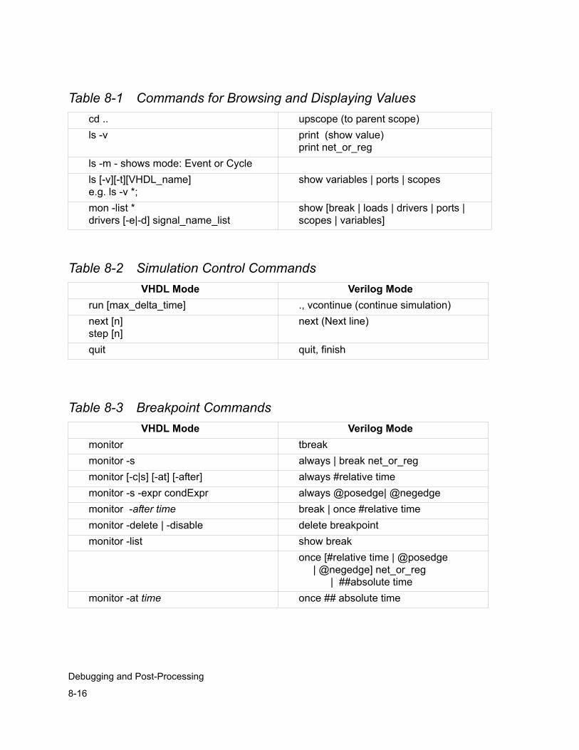
8-16
Debugging and Post-Processing
cd .. upscope (to parent scope)ls -v print (show value)
print net_or_regls -m - shows mode: Event or Cyclels [-v][-t][VHDL_name]e.g. ls -v *;
show variables | ports | scopes
mon -list *drivers [-e|-d] signal_name_list
show [break | loads | drivers | ports | scopes | variables]
Table 8-2 Simulation Control CommandsVHDL Mode Verilog Mode
run [max_delta_time] ., vcontinue (continue simulation)next [n]step [n]
next (Next line)
quit quit, finish
Table 8-3 Breakpoint CommandsVHDL Mode Verilog Mode
monitor tbreakmonitor -s always | break net_or_regmonitor [-c|s] [-at] [-after] always #relative time monitor -s -expr condExpr always @posedge| @negedgemonitor -after time break | once #relative timemonitor -delete | -disable delete breakpointmonitor -list show break
once [#relative time | @posedge | @negedge] net_or_reg | ##absolute time
monitor -at time once ## absolute time
Table 8-1 Commands for Browsing and Displaying Values
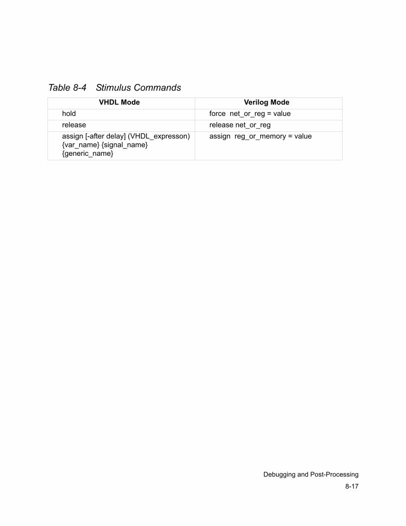
8-17
Debugging and Post-Processing
Table 8-4 Stimulus CommandsVHDL Mode Verilog Mode
hold force net_or_reg = valuerelease release net_or_regassign [-after delay] (VHDL_expresson){var_name} {signal_name} {generic_name}
assign reg_or_memory = value
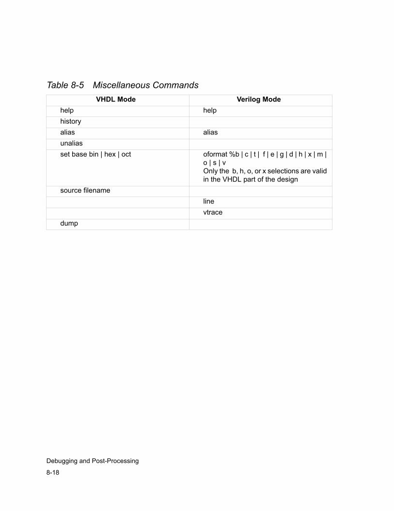
8-18
Debugging and Post-Processing
Table 8-5 Miscellaneous CommandsVHDL Mode Verilog Mode
help helphistoryalias aliasunaliasset base bin | hex | oct oformat %b | c | t | f | e | g | d | h | x | m |
o | s | vOnly the b, h, o, or x selections are valid in the VHDL part of the design
source filenamelinevtrace
dump
9-1
Discovery Visual Environment
9 Discovery Visual Environment 4
Discovery Visual Environment (DVE) software is a graphical verification environment that supports debugging for VCS MX simulations. DVE allows you to work in post-processing and interactive mode.
For information on using DVE, see the Discovery Visual Environment User Guide.
Using DVE, you can perform the following tasks:
• Hierarchically expand and view HDL scope information.
• Debug assertions.
• View log, history, and error/warning information related to your analysis.
9-2
Discovery Visual Environment
• Perform TCL tasks by executing scripts from the DVE graphical user interface or executing TCL commands or sourcing scripts through the command-line interface.
Primary DVE Components
This section provides an overview of the following core components of DVE:
• Top Level Window
• Source Window
• Assertion Window
• Wave Window
• List Window
• Schematic Window
Top Level Window
The Top Level Window is a frame that can contain the other windows. A Top Level Window has menus, toolbars and statusbar. From the Top Level Window, you can:
• Use the Menu bar, Toolbar, and Status Bar to run and interact with a simulation or open, view, navigate, edit, and close a design database and set the target for new panes and windows containing source code, waveforms, schematics, and ASCII data. You can specify analysis and search parameters, invoke TCL scripts, run examples, and access Help.
9-3
Discovery Visual Environment
• Use the Hierarchy Browser to view, expand, and select scopes of interest for display in a Waveform Window.
• View and filter signal information. Double click a signal of interest to view source code or drag and drop it into another DVE pane or window. Dragging and dropping is supported in the Data Pane, Source, Wave, List, and Assertion windows.
• View HDL or Assertion source code in the Source Window or in multiple Source Windows.
• View assertion failures and history.
• Perform TCL tasks by executing scripts from the DVE graphical user interface or executing TCL commands or sourcing scripts through the command-line interface.
• Activate any open DVE window or pane regardless of where it is in the desktop window stack.
• Access DVE windows, such as the Waveform Window and List Window, to debug your design.
Figure 9-1 shows an example of the Top Level Window.
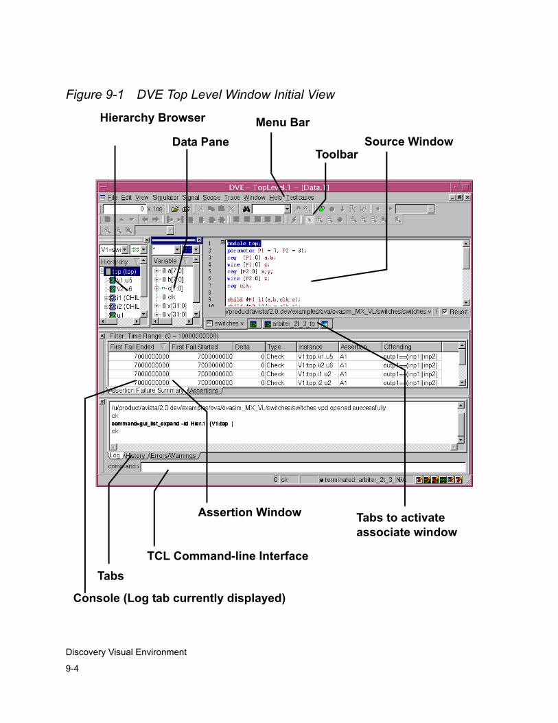
9-4
Discovery Visual Environment
Figure 9-1 DVE Top Level Window Initial View
Menu Bar
Toolbar
Hierarchy Browser
Source Window
Tabs
Console (Log tab currently displayed)
TCL Command-line Interface
Data Pane
Tabs to activate associate window
Assertion Window
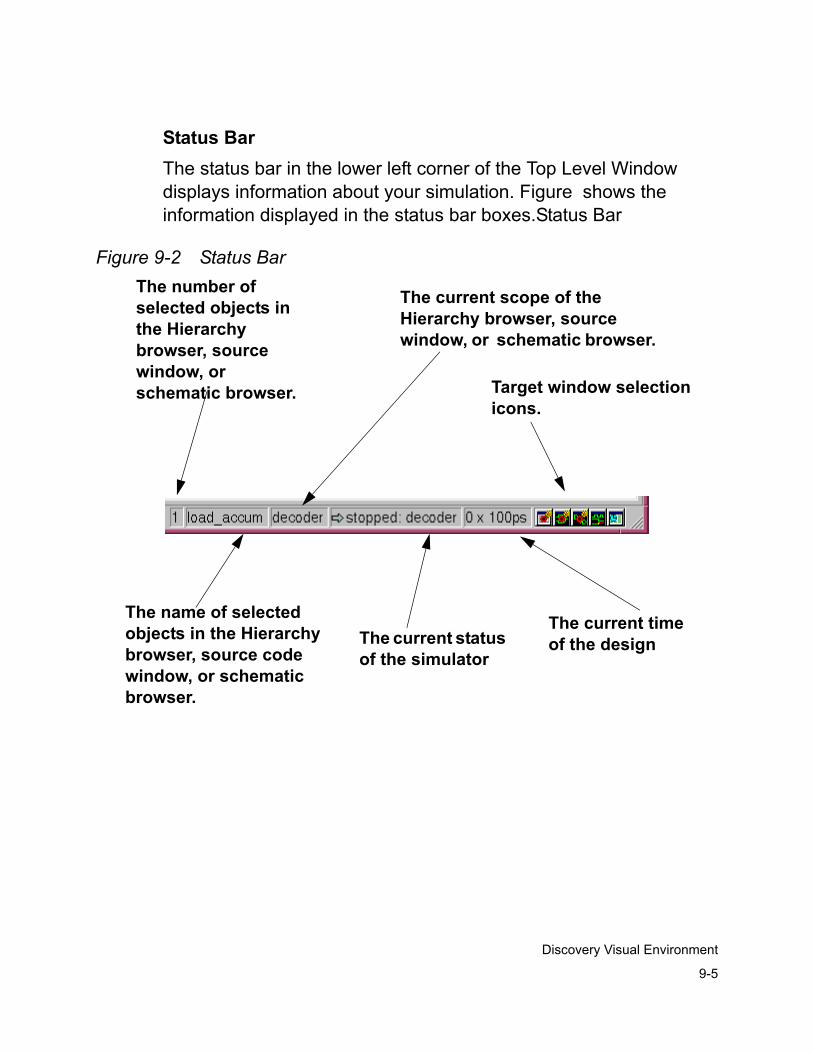
9-5
Discovery Visual Environment
Status BarThe status bar in the lower left corner of the Top Level Window displays information about your simulation. Figure shows the information displayed in the status bar boxes.Status Bar
Figure 9-2 Status BarThe number of selected objects in the Hierarchy browser, source window, or schematic browser.
The name of selected objects in the Hierarchy browser, source code window, or schematic browser.
The current scope of the Hierarchy browser, source window, or schematic browser.
The current time of the design The current status
of the simulator
Target window selection icons.
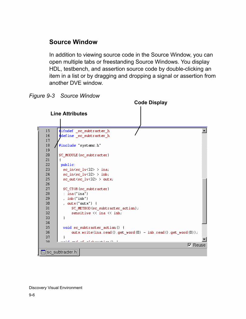
9-6
Discovery Visual Environment
Source Window
In addition to viewing source code in the Source Window, you can open multiple tabs or freestanding Source Windows. You display HDL, testbench, and assertion source code by double-clicking an item in a list or by dragging and dropping a signal or assertion from another DVE window.
Figure 9-3 Source Window
Line Attributes
Code Display
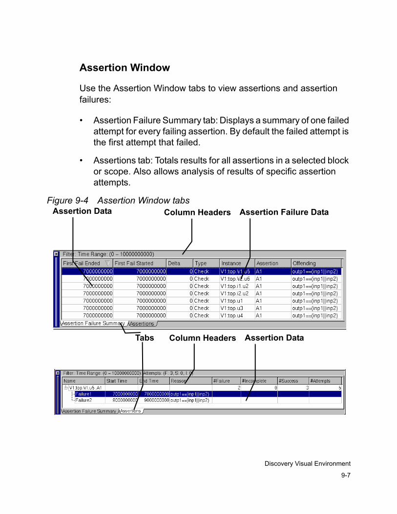
9-7
Discovery Visual Environment
Assertion Window
Use the Assertion Window tabs to view assertions and assertion failures:
• Assertion Failure Summary tab: Displays a summary of one failed attempt for every failing assertion. By default the failed attempt is the first attempt that failed.
• Assertions tab: Totals results for all assertions in a selected block or scope. Also allows analysis of results of specific assertion attempts.
Figure 9-4 Assertion Window tabsAssertion Data Assertion Failure DataColumn Headers
Assertion DataColumn HeadersTabs
9-8
Discovery Visual Environment
Wave Window
The Wave Window displays
• Waveforms of selected signals in your design.
• Trace information for a particular assertion, along with a waveform of the signals and expressions associated with the assertion.
Displaying Signals in the Wave WindowUse the Wave Window to view and highlight signals of interest, advance to various simulation times, and view simulation time deltas.
To view signals in the Waveform Window, you can double click an an assertion summary item or an attempt, drag and drop an item in a list or select an item and select Add to Waves from the menu.
Figure 9-5 shows an example of the Waveform Window displaying signals. Cursor 1 (C1) indicates current time.
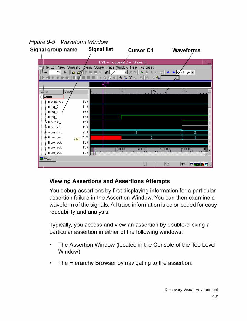
9-9
Discovery Visual Environment
Figure 9-5 Waveform Window
Viewing Assertions and Assertions AttemptsYou debug assertions by first displaying information for a particular assertion failure in the Assertion Window, You can then examine a waveform of the signals. All trace information is color-coded for easy readability and analysis.
Typically, you access and view an assertion by double-clicking a particular assertion in either of the following windows:
• The Assertion Window (located in the Console of the Top Level Window)
• The Hierarchy Browser by navigating to the assertion.
Signal list Cursor C1 Waveforms Signal group name
9-10
Discovery Visual Environment
Or you can drag and drop an OVA assertion unit from the Hierarchy Browser or an OVA or SVA assertion from the Data Window into the the Wave Window (double click to display the source code in the Source Window).
You can then view a trace of a failed assertion by double clicking a failed attempt (a red up arrow) in the Wave Window.
Figure 9-6 shows an example of the Waveform Window. displaying a trace of a failed assertion attempt. The cursors mark the start and end times of the failure and the background color is also different to indicate the assertion time region. This lighter color persists if the cursors are moved to make it easy to identify the assertion region.

9-11
Discovery Visual Environment
Figure 9-6 Waveform Window displaying a trace of a failed assertion attempt
List Window
Use the List Window to generate ASCII simulation results. The List Window displays simulation data as shown in the Wave Window but in tabular format. It is a scrollable window, showing simulation time on the left.
Start time ofassertion failure
End time ofassertion failure
Assertion and related signals
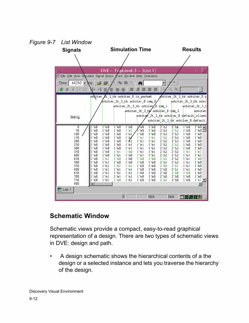
9-12
Discovery Visual Environment
Figure 9-7 List Window
Schematic Window
Schematic views provide a compact, easy-to-read graphical representation of a design. There are two types of schematic views in DVE: design and path.
• A design schematic shows the hierarchical contents of a the design or a selected instance and lets you traverse the hierarchy of the design.
Signals Simulation Time Results
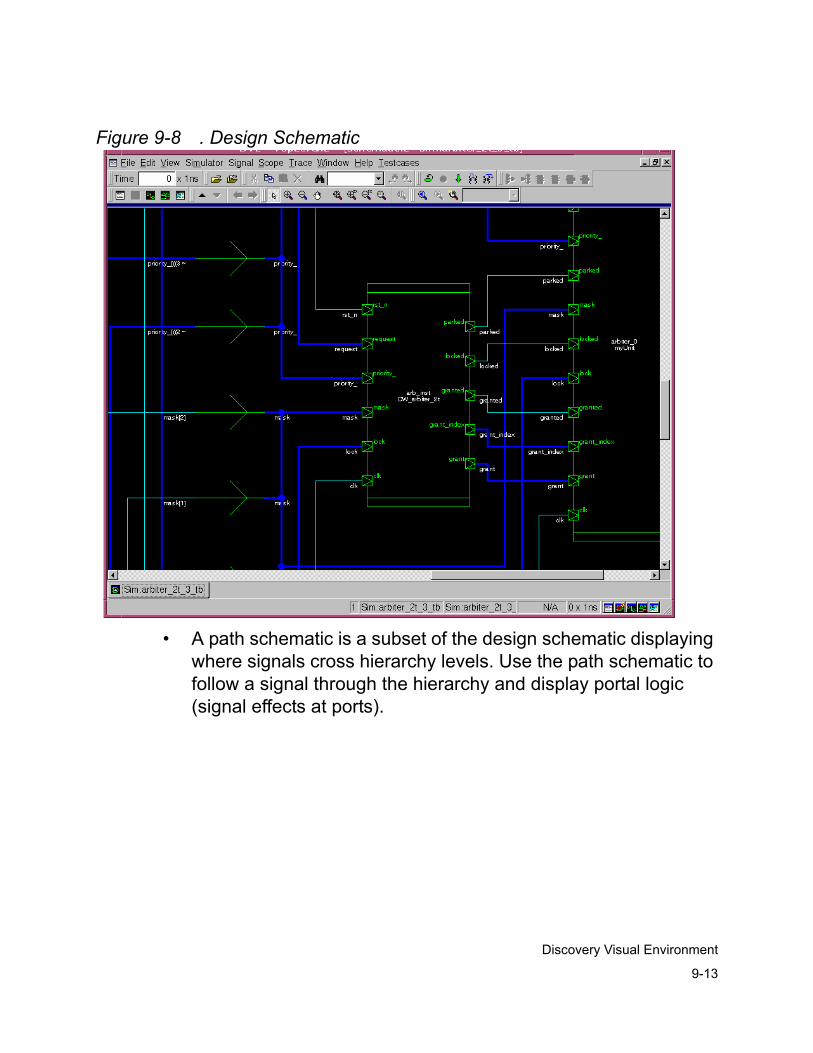
9-13
Discovery Visual Environment
Figure 9-8 . Design Schematic
• A path schematic is a subset of the design schematic displaying where signals cross hierarchy levels. Use the path schematic to follow a signal through the hierarchy and display portal logic (signal effects at ports).
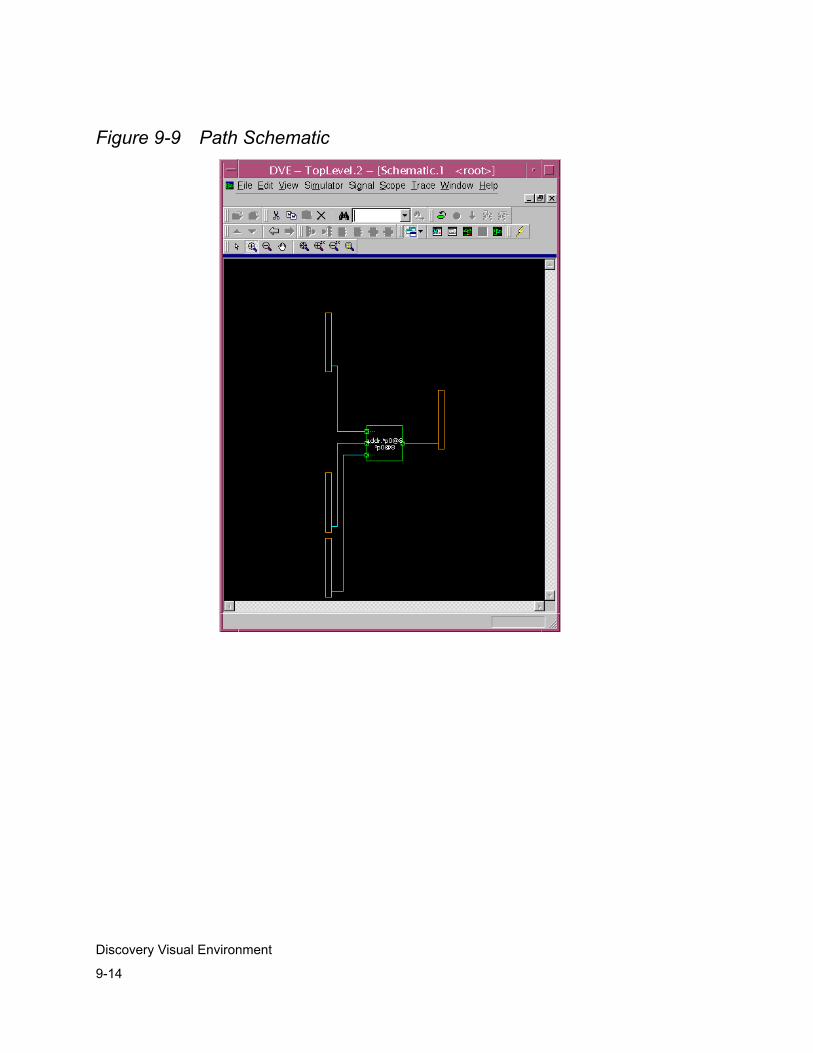
9-14
Discovery Visual Environment
Figure 9-9 Path Schematic
10-1
Using OpenVera Assertions
10Using OpenVera Assertions 5
This chapter introduces OpenVera Assertions, and explains how to compile and run OpenVera Assertions within the various VCS MX flows.
This chapter cover the following topics:
• Introducing OpenVera Assertions
• Creating a Temporal Assertion File
• Compiling Temporal Assertions Files
• OVA Runtime Options
• Using OVA with VHDL-Only and Mixed-HDL Designs
• Viewing OVA Simulation Results
10-2
Using OpenVera Assertions
Introducing OpenVera Assertions
OpenVera Assertions (OVA) provides a clear, easy way to describe sequences of events and facilities to test for their occurrence. With clear definitions and less code, testbench design is faster and easier. And you can be confident that you are testing the right sequences in the right way.
OVA is a clear, easy way to describe sequences of events and facilities to test for their occurrence. With clear definitions and less code, testbench design is faster and easier, and you can be confident that you are testing the right sequences in the right way.
As a declarative method, OVA is much more concise and easier to read than the procedural descriptions provided by hardware description languages such as Verilog. With OVA:
• Descriptions can range from the most simple to the most complex logical and conditional combinations.
• Sequences can specify precise timing or a range of times.
• Descriptions can be associated with specified modules and module instances.
• Descriptions can be grouped as a library for repeated use. OVA includes a Checker Library of commonly used descriptions.
10-3
Using OpenVera Assertions
Built-in Test Facilities and Functions
OVA has built-in test facilities to minimize the amount of code that you need to write. In addition, OVA works seamlessly with other Synopsys tools to form a complete verification environment. OVA performs the following tasks:
• Tests Verilog, VHDL, and mixed-HDL designs using VCS-MX.
• Automatically tests and reports results on all defined sequences. You just write the definitions.
• Produces results that can be viewed with DVE or VirSim.
• Can be monitored and controlled as part of a Vera testbench.
For more information on OVA, see the OpenVera Language Reference Manual: Assertions.
Creating a Temporal Assertion File
Testing starts with a temporal assertion file, which contains the descriptions of the sequences and instructions for how they should be tested.
A typical temporal assertion file consists mostly of temporal expressions, which are the descriptions of the event sequences.
The basic instruction for testing is a temporal assertion. Assertions specify an expression or combination of expressions to be tested. Assertions come in two forms: check, which succeeds when the simulation matches the expression, and forbid, which succeeds when the simulation does not match.
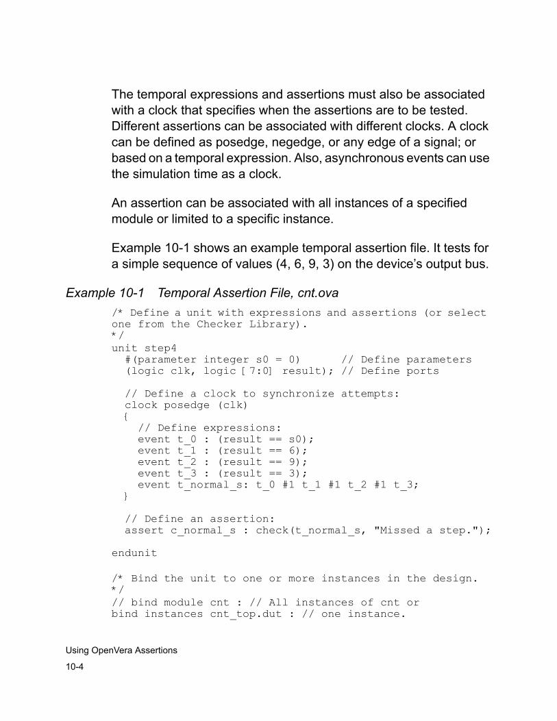
10-4
Using OpenVera Assertions
The temporal expressions and assertions must also be associated with a clock that specifies when the assertions are to be tested. Different assertions can be associated with different clocks. A clock can be defined as posedge, negedge, or any edge of a signal; or based on a temporal expression. Also, asynchronous events can use the simulation time as a clock.
An assertion can be associated with all instances of a specified module or limited to a specific instance.
Example 10-1 shows an example temporal assertion file. It tests for a simple sequence of values (4, 6, 9, 3) on the device’s output bus.
Example 10-1 Temporal Assertion File, cnt.ova/* Define a unit with expressions and assertions (or select one from the Checker Library).*/unit step4
#(parameter integer s0 = 0) // Define parameters(logic clk, logic [7:0] result); // Define ports
// Define a clock to synchronize attempts: clock posedge (clk)
{ // Define expressions: event t_0 : (result == s0); event t_1 : (result == 6); event t_2 : (result == 9); event t_3 : (result == 3); event t_normal_s: t_0 #1 t_1 #1 t_2 #1 t_3; }
// Define an assertion: assert c_normal_s : check(t_normal_s, "Missed a step.");
endunit
/* Bind the unit to one or more instances in the design.*/// bind module cnt : // All instances of cnt orbind instances cnt_top.dut : // one instance.
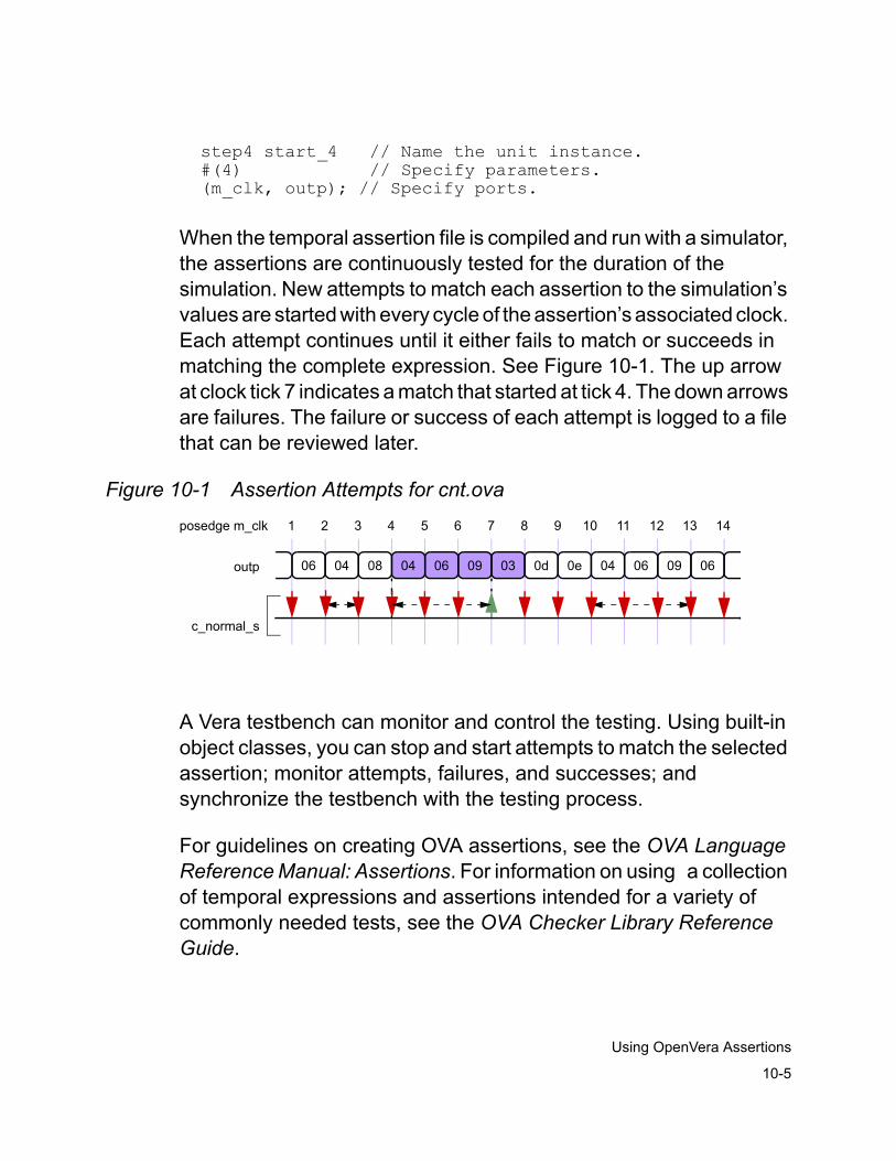
10-5
Using OpenVera Assertions
step4 start_4 // Name the unit instance.#(4) // Specify parameters.(m_clk, outp); // Specify ports.
When the temporal assertion file is compiled and run with a simulator, the assertions are continuously tested for the duration of the simulation. New attempts to match each assertion to the simulation’s values are started with every cycle of the assertion’s associated clock. Each attempt continues until it either fails to match or succeeds in matching the complete expression. See Figure 10-1. The up arrow at clock tick 7 indicates a match that started at tick 4. The down arrows are failures. The failure or success of each attempt is logged to a file that can be reviewed later.
Figure 10-1 Assertion Attempts for cnt.ova
A Vera testbench can monitor and control the testing. Using built-in object classes, you can stop and start attempts to match the selected assertion; monitor attempts, failures, and successes; and synchronize the testbench with the testing process.
For guidelines on creating OVA assertions, see the OVA Language Reference Manual: Assertions. For information on using a collection of temporal expressions and assertions intended for a variety of commonly needed tests, see the OVA Checker Library Reference Guide.
1 2 3 4 5 6 7 8 9 10 11 12 13 14posedge m_clk
outp
c_normal_s
06 04 0408 06 09 03 0d 0e 04 06 09 06
10-6
Using OpenVera Assertions
Compiling Temporal Assertions Files
Temporal assertions files are compiled concurrently with Verilog source files. You can use a set of OVA-specific compile-time options to control how VCS compiles the temporal assertions files.
Note:When you use the OVA compile-time options, VCS creates a Verification Database directory in your current directory (by default named simv.vdb). VCS writes intermediate files and reports about OpenVera Assertions in subdirectories within in this directory.
The following compile-time options are for OVA:
-ova_covEnables viewing results with functional coverage.
-ova_cov_eventsEnables coverage reporting of expressions.
-ova_cov_hier filenameLimits functional coverage to the module instances specified in filename. Specify the instances using the same format as VCS coverage metrics. If this option is not used, coverage is implemented on the whole design.
-ova_debug | -ova_debug_vpdRequired to view results with DVE or VirSim.
10-7
Using OpenVera Assertions
-ova_dir pathnameSpecifies an alternative name and location for the Verification Database directory. There is no need to specify the name and location of the new Verification Database directory at runtime, the simv executable contains this information.
If you move or rename this directory after you create the simv executable, you include this option at runtime to tell VCS its new name or location.
-ova_file filenameIdentifies filename as an assertion file. Not required if the file name ends with .ova. For multiple assertion files, repeat this option with each file.
-ova_enable_diagEnables further control of result reporting with runtime options.
-ova_inlineEnables compiling of OVA code that is written inline with a Verilog design.
Note:You can also use the VCS -f option to specify a file containing a list of all absolute pathnames for Verilog source files and compile-time option. You can pass all OVA compile-time options through this file, except -ova_debug.
10-8
Using OpenVera Assertions
OVA Runtime Options
The following runtime options are available for use with OVA:
-ova_quiet [1]Disables printing results on screen. The report file is not affected. With the 1 argument, only a summary is printed on screen.
-ova_report [filename]Generates a report file in addition to printing results on screen. Specifying the full path name of the report file overrides the default report name and location.
-ova_verboseAdds more information to the end of the report including assertions that never triggered and attempts that did not finish, and a summary with the number of assertions present, attempted, and failed.
A set of runtime options are also available for controlling how VCS writes its report on OpenVera Assertions. You can use these options only if you compiled with the -ova_enable_diag compile-time option.
-ova_filterBlocks reporting of trivial if-then successes. These happen when an if-then construct registers a success only because the if portion is false (and so the then portion is not checked). With this option, reporting only shows successes in which the whole expression matched.
ova_filter_pastIgnores assertion subsequences containing past operators that have not yet eclipsed the history threshold.
10-9
Using OpenVera Assertions
-ova_max_fail NLimits the number of failures for each assertion to N. When the limit is reached, the assertion is disabled. N must be supplied, otherwise no limit is set.
-ova_max_success NLimits the total number of reported successes to N. N must be supplied, otherwise no limit is set. The monitoring of assertions continues, even after the limit is reached.
-ova_simend_max_fail NTerminates the simulation if the number of failures for any assertion reaches N. N must be supplied, otherwise no limit is set.
-ova_successEnables reporting of successful matches in addition to failures. The default is to report only failures.
Using OVA with VHDL-Only and Mixed-HDL Designs
This section shows you how to run OVA with VHDL-Only and Mixed-HDL designs. For details on running OVA with Verilog-Only designs, see the VCS User Guide.
1. In addition to setting up your normal environment, (see “Setting Up Your Environment” on page 1-3), set the LD_LIBRARY_PATH environment variable:
setenv LD_LIBRARY_PATH $VCS_HOME/<platform>/lib:$LD_LIBRARY_PATH
Note: For HP configurations, set SHLIB_PATH instead of LD_LIBRARY_PATH.
2. Make sure you’ve already created an OVA temporal assertons file or files (see “Creating a Temporal Assertion File” on page 5-3).
10-10
Using OpenVera Assertions
3. Compile the OVA code using the ovaan utility:
ovaan chk_clkgen.ova
Note the following:
- All OVA files must be specified at the same command line.
- For details on the ovaan utility, see “ovaan Utility” on page 3-15 of the VCS MX Reference Guide.
4. Analyze the HDL source code using either the vhdlan utility (for VHDL) or vlogan utility (for Verilog):
vhdlan design.vhd other_compile_files_and_options
vlogan design.v other_compile_files_and_options
For details on the vhdlan utility, see “vhdlan Utility” on page 3-2 of the VCS MX Reference Guide. For details on the vlogan utility, see “vlogan Utility” on page 3-10 of the VCS MX Reference Guide.
5. Compile the design and OVA code:
- For VHDL-Only designs, use the scs command and -ova option.
scs cfg_tb -ova
- For VHDL-Top designs, use the scs command and -mhdl and -ova options.
scs -mhdl cfg_tb -ova
For details on the scs command, please see “scs Command and Options” on page 4-2 of the VCS MX Reference Guide.
10-11
Using OpenVera Assertions
- For Verilog-Top, use the vcs command and -mhdl and -ova options.
vcs -mhdl -ova tb.v
For details on the vcs command, see “vcs Command and Options” on page 4-11 of the VCS MX Reference Guide.
6. Run your simulation using the scsim executable and -ovarun flag for VHDL-Only and VHDL-Top, or the simv executable and -ovarun for Verilog-Top.
scsim -ovarun "ova_runtime_flags"
simv -ovarun "ova_runtime_flags"
For details on the scsim executable, see “scsim Executable and Options” on page 5-1 of the VCS MX Reference Guide. For details on the simv executable, see “simv Executable and Options” on page 5-11 of the VCS MX Reference Guide.
7. In addition to the simulation’s usual output, you will get a report of the OVA results. For details on these reports, see “Viewing OVA Simulation Results” on page 5-11.
Viewing OVA Simulation Results
You can view OVA simulations results in different ways based on the options you used with the ovaan utility or -ovarun.
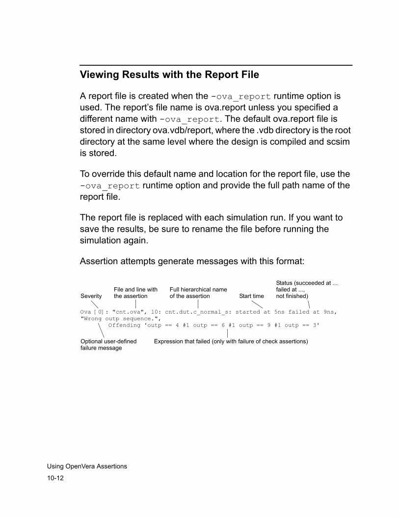
10-12
Using OpenVera Assertions
Viewing Results with the Report File
A report file is created when the -ova_report runtime option is used. The report’s file name is ova.report unless you specified a different name with -ova_report. The default ova.report file is stored in directory ova.vdb/report, where the .vdb directory is the root directory at the same level where the design is compiled and scsim is stored.
To override this default name and location for the report file, use the -ova_report runtime option and provide the full path name of the report file.
The report file is replaced with each simulation run. If you want to save the results, be sure to rename the file before running the simulation again.
Assertion attempts generate messages with this format:
Ova [0]: "cnt.ova", 10: cnt.dut.c_normal_s: started at 5ns failed at 9ns,
File and line withthe assertion
Full hierarchical nameof the assertion
Status (succeeded at ...,failed at ...,not finished)
Optional user-definedfailure message
Expression that failed (only with failure of check assertions)
"Wrong outp sequence.",Offending 'outp == 4 #1 outp == 6 #1 outp == 9 #1 outp == 3'
Start timeSeverity
10-13
Using OpenVera Assertions
Viewing Results with Functional Coverage
After running simulations, you can generate a report summarizing the coverage of the assertions and expressions. With this report you can quickly see if all assertions were attempted, how often they were successful, and how often they failed. Potential problem areas can be easily identified. The report can cover one test or merge the results of a test suite. The report is presented in HTML and you can customize it with a TCL script.
The default report shows the number of assertions and expressions that:
• were attempted
• had successes
• had failures
Coverage is broken down by module and instance, showing for each assertion and expression, the number of attempts, failures, and successes. Because if-then constructs register a success anytime the if portion is false (and so the then portion is not checked), the report also shows the number of real successes in which the whole expression matched. This works with nested if statements too.
Functional coverage can also grade the effectiveness of tests, producing a list of the minimum set of tests that meet the coverage target. Tests can be graded on any of these metrics:
• number of successful assertion attempts versus number of assertions (metric = SN)
• number of failed assertion attempts versus number of assertions (metric = FN)
10-14
Using OpenVera Assertions
• number of assertion attempts versus number of assertions (metric = AN)
• number of successful assertion attempts versus number of assertion attempts (metric = SA)
• number of failed assertion attempts versus number of assertion attempts (metric = FA)
To generate a report run the following command:
fcovReport [options]
For a description of the command options, see Table 10-1.
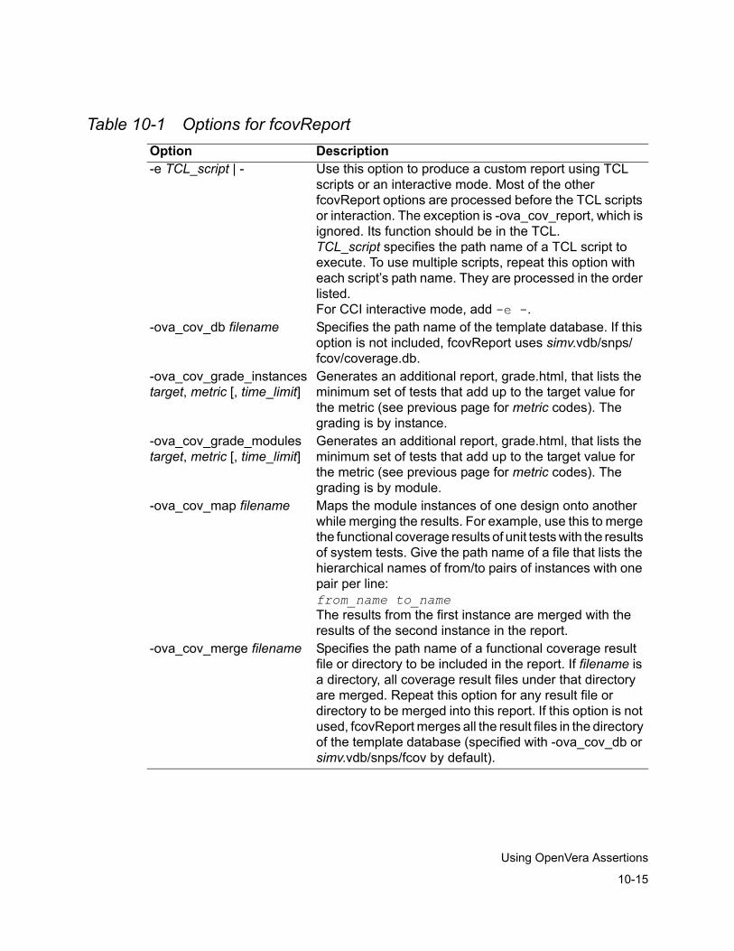
10-15
Using OpenVera Assertions
Table 10-1 Options for fcovReportOption Description-e TCL_script | - Use this option to produce a custom report using TCL
scripts or an interactive mode. Most of the other fcovReport options are processed before the TCL scripts or interaction. The exception is -ova_cov_report, which is ignored. Its function should be in the TCL.TCL_script specifies the path name of a TCL script to execute. To use multiple scripts, repeat this option with each script’s path name. They are processed in the order listed.For CCI interactive mode, add -e -.
-ova_cov_db filename Specifies the path name of the template database. If this option is not included, fcovReport uses simv.vdb/snps/fcov/coverage.db.
-ova_cov_grade_instances target, metric [, time_limit]
Generates an additional report, grade.html, that lists the minimum set of tests that add up to the target value for the metric (see previous page for metric codes). The grading is by instance.
-ova_cov_grade_modules target, metric [, time_limit]
Generates an additional report, grade.html, that lists the minimum set of tests that add up to the target value for the metric (see previous page for metric codes). The grading is by module.
-ova_cov_map filename Maps the module instances of one design onto another while merging the results. For example, use this to merge the functional coverage results of unit tests with the results of system tests. Give the path name of a file that lists the hierarchical names of from/to pairs of instances with one pair per line:from_name to_nameThe results from the first instance are merged with the results of the second instance in the report.
-ova_cov_merge filename Specifies the path name of a functional coverage result file or directory to be included in the report. If filename is a directory, all coverage result files under that directory are merged. Repeat this option for any result file or directory to be merged into this report. If this option is not used, fcovReport merges all the result files in the directory of the template database (specified with -ova_cov_db or simv.vdb/snps/fcov by default).

10-16
Using OpenVera Assertions
You can produce a custom report with TCL. See Table 10-2 for extra TCL commands for functional coverage.
-ova_cov_report name | path/name
Specifies the base name for the report.The fcovReport command creates an HTML index file at simv.vdb/reports/name.fcov-index.html and stores the other report files under simv.vdb/reports/name.fcov.If you give a path name, the last component of the path is used as the base name. So the report files are stored under path/name and the index file is at path/name.fcov-index.html.If this option is not included, the report files are stored under simv.vdb/reports/report.fcov and the index file is named report.fcov-index.html.
Option Description
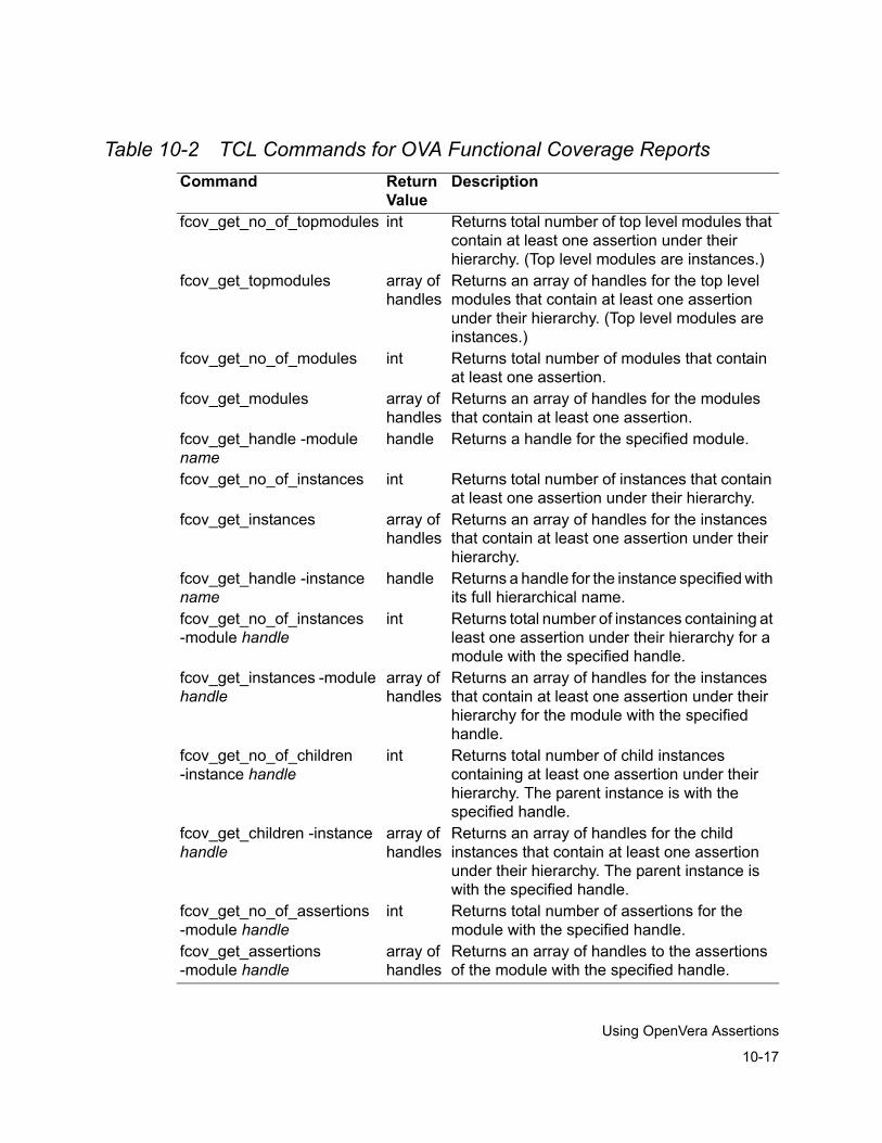
10-17
Using OpenVera Assertions
Table 10-2 TCL Commands for OVA Functional Coverage ReportsCommand Return
ValueDescription
fcov_get_no_of_topmodules int Returns total number of top level modules that contain at least one assertion under their hierarchy. (Top level modules are instances.)
fcov_get_topmodules array of handles
Returns an array of handles for the top level modules that contain at least one assertion under their hierarchy. (Top level modules are instances.)
fcov_get_no_of_modules int Returns total number of modules that contain at least one assertion.
fcov_get_modules array of handles
Returns an array of handles for the modules that contain at least one assertion.
fcov_get_handle -module name
handle Returns a handle for the specified module.
fcov_get_no_of_instances int Returns total number of instances that contain at least one assertion under their hierarchy.
fcov_get_instances array of handles
Returns an array of handles for the instances that contain at least one assertion under their hierarchy.
fcov_get_handle -instance name
handle Returns a handle for the instance specified with its full hierarchical name.
fcov_get_no_of_instances -module handle
int Returns total number of instances containing at least one assertion under their hierarchy for a module with the specified handle.
fcov_get_instances -module handle
array of handles
Returns an array of handles for the instances that contain at least one assertion under their hierarchy for the module with the specified handle.
fcov_get_no_of_children -instance handle
int Returns total number of child instances containing at least one assertion under their hierarchy. The parent instance is with the specified handle.
fcov_get_children -instance handle
array of handles
Returns an array of handles for the child instances that contain at least one assertion under their hierarchy. The parent instance is with the specified handle.
fcov_get_no_of_assertions -module handle
int Returns total number of assertions for the module with the specified handle.
fcov_get_assertions -module handle
array of handles
Returns an array of handles to the assertions of the module with the specified handle.
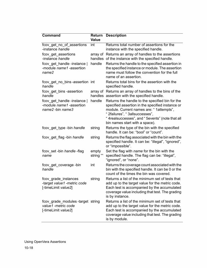
10-18
Using OpenVera Assertions
fcov_get_no_of_assertions -instance handle
int Returns total number of assertions for the instance with the specified handle.
fcov_get_assertions -instance handle
array of handles
Returns an array of handles to the assertions of the instance with the specified handle.
fcov_get_handle -instance | -module name1 -assertion name2
handle Returns the handle to the specified assertion in the specified instance or module. The assertion name must follow the convention for the full name of an assertion.
fcov_get_no_bins -assertion handle
int Returns total bins for the assertion with the specified handle.
fcov_get_bins -assertion handle
array of handles
Returns an array of handles to the bins of the assertion with the specified handle.
fcov_get_handle -instance | -module name1 -assertion name2 -bin name3
handle Returns the handle to the specified bin for the specified assertion in the specified instance or module. Current names are: “ 1attempts”, “ 2failures”, “ 3allsuccesses”, “ 4realsuccesses”, and “ 5events” (note that all bin names start with a space).
fcov_get_type -bin handle string Returns the type of the bin with the specified handle. It can be: “bool” or “count”.
fcov_get_flag -bin handle string Returns the flag associated with the bin with the specified handle. It can be: “illegal”, “ignored”, or “impossible”.
fcov_set -bin handle -flag name
empty string ““
Set the flag with name for the bin with the specified handle. The flag can be: “illegal”, “ignored”, or “none”.
fcov_get_coverage -bin handle
int Returns the coverage count associated with the bin with the specified handle. It can be 0 or the count of the times the bin was covered.
fcov_grade_instances -target value1 -metric code [-timeLimit value2]
string Returns a list of the minimum set of tests that add up to the target value for the metric code. Each test is accompanied by the accumulated coverage value including that test. The grading is by instance.
fcov_grade_modules -target value1 -metric code [-timeLimit value2]
string Returns a list of the minimum set of tests that add up to the target value for the metric code. Each test is accompanied by the accumulated coverage value including that test. The grading is by module.
Command Return Value
Description
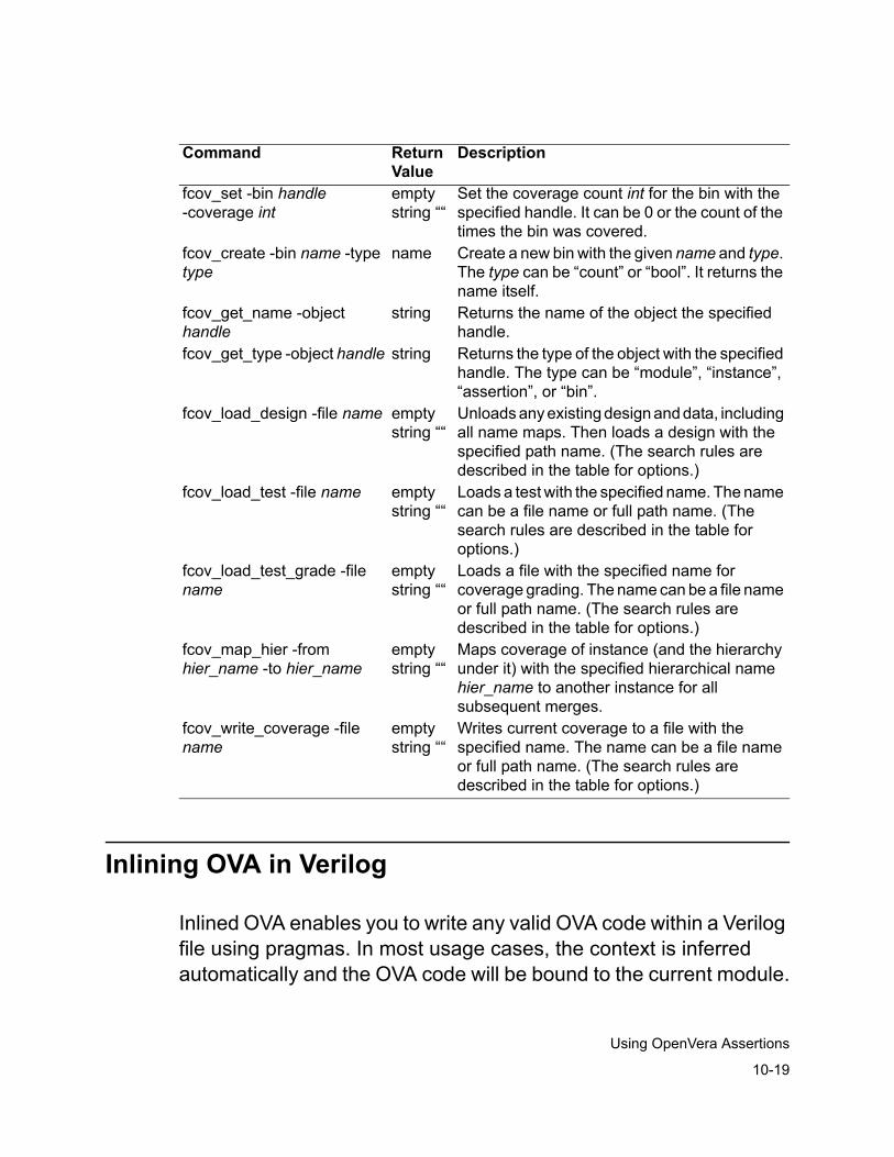
10-19
Using OpenVera Assertions
Inlining OVA in Verilog
Inlined OVA enables you to write any valid OVA code within a Verilog file using pragmas. In most usage cases, the context is inferred automatically and the OVA code will be bound to the current module.
fcov_set -bin handle -coverage int
empty string ““
Set the coverage count int for the bin with the specified handle. It can be 0 or the count of the times the bin was covered.
fcov_create -bin name -type type
name Create a new bin with the given name and type. The type can be “count” or “bool”. It returns the name itself.
fcov_get_name -object handle
string Returns the name of the object the specified handle.
fcov_get_type -object handle string Returns the type of the object with the specified handle. The type can be “module”, “instance”, “assertion”, or “bin”.
fcov_load_design -file name empty string ““
Unloads any existing design and data, including all name maps. Then loads a design with the specified path name. (The search rules are described in the table for options.)
fcov_load_test -file name empty string ““
Loads a test with the specified name. The name can be a file name or full path name. (The search rules are described in the table for options.)
fcov_load_test_grade -file name
empty string ““
Loads a file with the specified name for coverage grading. The name can be a file name or full path name. (The search rules are described in the table for options.)
fcov_map_hier -from hier_name -to hier_name
empty string ““
Maps coverage of instance (and the hierarchy under it) with the specified hierarchical name hier_name to another instance for all subsequent merges.
fcov_write_coverage -file name
empty string ““
Writes current coverage to a file with the specified name. The name can be a file name or full path name. (The search rules are described in the table for options.)
Command Return Value
Description
10-20
Using OpenVera Assertions
You can use this process with or without regular OVA files. The results for both inlined and regular (OVA) assertions are reported together.
All Verilog files containing inlined OVAs are passed to the ovaan utility using the -ova_inline command line switch.
This section covers the following topics:
• “Specifying Pragmas in Verilog
• “Methods for Inlining OVA
• “General Inlined OVA Coding Guidelines
Specifying Pragmas in VerilogInlined OVA is specified in Verilog code using pragmas. Several different forms are accepted, including C and C++ style comments, and modified C++ multi-line comments.
The general C++ style form is as follows:
/* ova first_part_of_pragma...last_part_of_pragma*/
You can also use the following modified C++ approach:
//ova_begin// pragma_statement//...//ova_end
10-21
Using OpenVera Assertions
For a single-line pragma, you can use the following C form:
// ova pragma_statement;
Assertions can be placed anywhere in a Verilog module and they use predefined units, including those in the Checker Library.
Note that the following OVA pragmas are not supported
• // ova parallel_case on;
• // ova full_case on;
• // ova inherit_clock;
Methods for Inlining OVA
There are four basic methods you can use to inline OVA within Verilog:
• Unit Instantiation Using the Unit-based Checker Library (recommended for using Synopsys-developed OVA checkers)
• Context-Independent Full Custom OVA (uses custom-developed OVA code that resides in a Verilog file)
• Template Instantiation Using the Template-Based Checker Library
• Context-Dependent Full Custom OVA
These methods are described in detail throughout this section. The graphic in Figure 10-2 provides an overview of these methods.
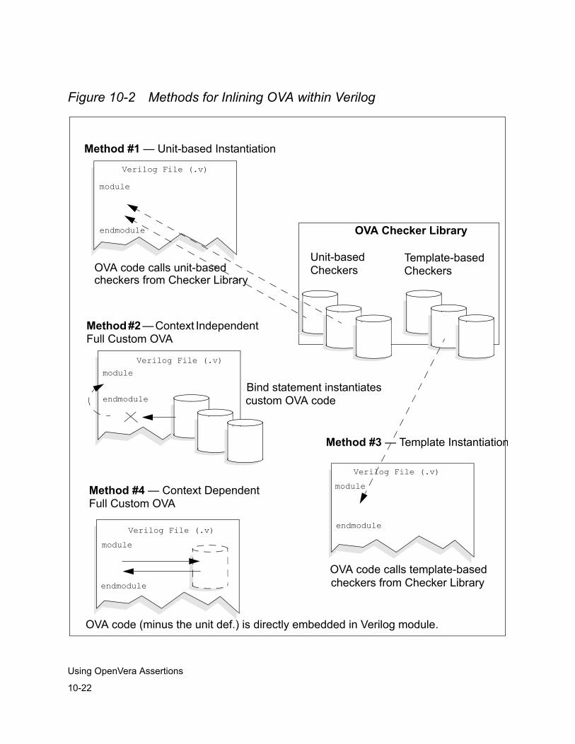
10-22
Using OpenVera Assertions
Figure 10-2 Methods for Inlining OVA within Verilog
OVA Checker Library
Method #1 — Unit-based Instantiation
Method #2 — Context Independent Full Custom OVA
Method #3 — Template Instantiation
Method #4 — Context Dependent Full Custom OVA
Unit-basedCheckers
Template-basedCheckersOVA code calls unit-based
Bind statement instantiatescustom OVA code
checkers from Checker Library
OVA code calls template-based checkers from Checker Library
OVA code (minus the unit def.) is directly embedded in Verilog module.
Verilog File (.v)
Verilog File (.v)
Verilog File (.v)
Verilog File (.v)
module
endmodule
module
endmodule
module
endmodule
module
endmodule
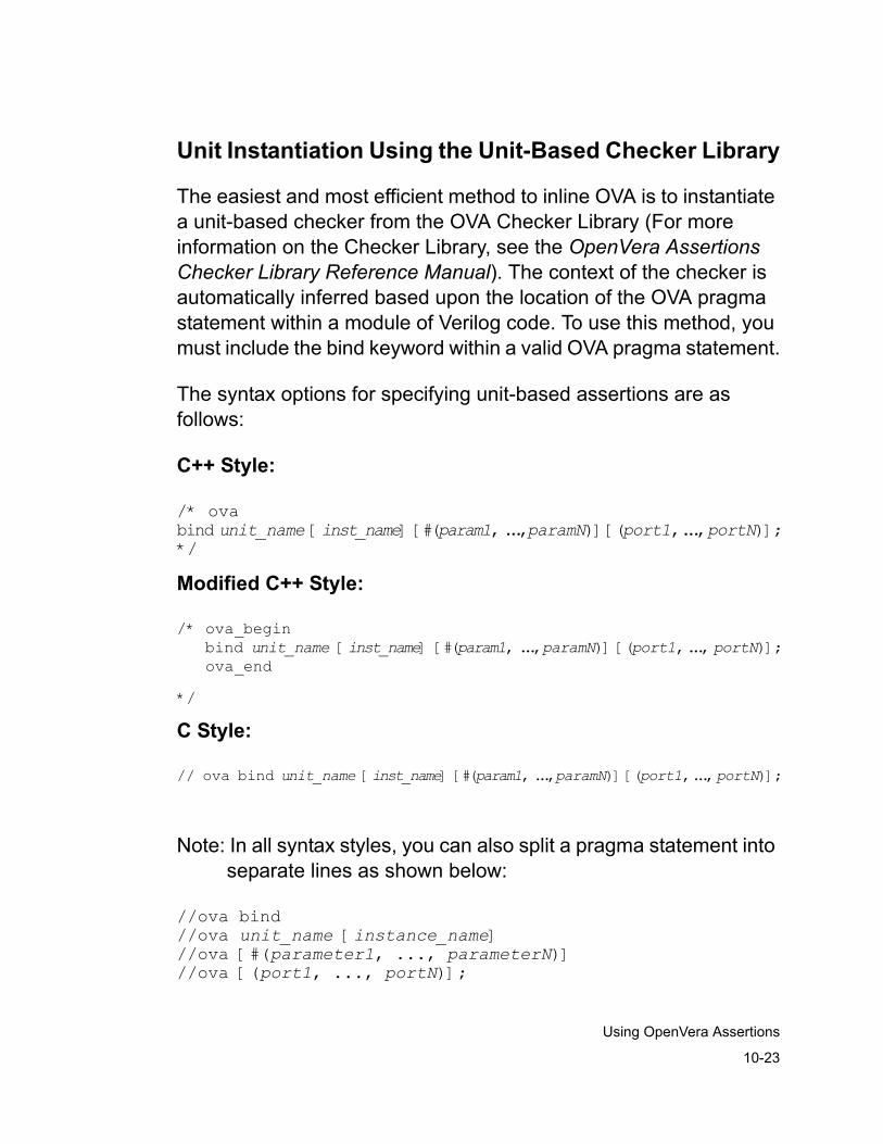
10-23
Using OpenVera Assertions
Unit Instantiation Using the Unit-Based Checker Library
The easiest and most efficient method to inline OVA is to instantiate a unit-based checker from the OVA Checker Library (For more information on the Checker Library, see the OpenVera Assertions Checker Library Reference Manual). The context of the checker is automatically inferred based upon the location of the OVA pragma statement within a module of Verilog code. To use this method, you must include the bind keyword within a valid OVA pragma statement.
The syntax options for specifying unit-based assertions are as follows:
C++ Style:
/* ova bind unit_name [inst_name] [#(param1, ..., paramN)] [(port1, ..., portN)];*/
Modified C++ Style:
/* ova_begin bind unit_name [inst_name] [#(param1, ..., paramN)] [(port1, ..., portN)]; ova_end
*/
C Style:
// ova bind unit_name [inst_name] [#(param1, ..., paramN)] [(port1, ..., portN)];
Note: In all syntax styles, you can also split a pragma statement into separate lines as shown below:
//ova bind//ova unit_name [instance_name]//ova [#(parameter1, ..., parameterN)]//ova [(port1, ..., portN)];
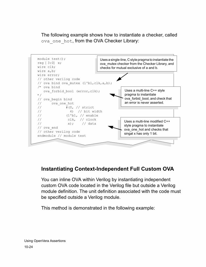
10-24
Using OpenVera Assertions
The following example shows how to instantiate a checker, called ova_one_hot, from the OVA Checker Library:
Instantiating Context-Independent Full Custom OVA
You can inline OVA within Verilog by instantiating independent custom OVA code located in the Verilog file but outside a Verilog module definition. The unit definition associated with the code must be specified outside a Verilog module.
This method is demonstrated in the following example:
module test();reg [3:0] x; wire clk; wire a,b; wire error; // other verilog code// ova bind ova_mutex (1'b1,clk,a,b); /* ova bind ova_forbid_bool (error,clk); */// ova_begin bind// ova_one_hot // #(0, // strict// 4) // bit width// (1'b1, // enable// clk, // clock // x); // data// ova_end// other verilog codeendmodule // module test
Uses a single-line, C style pragma to instantiate the ova_mutex checker from the Checker Library, and checks for mutual exclusive of a and b.
Uses a multi-line C++ style pragma to instantiate ova_forbid_bool, and check that an error is never asserted.
Uses a multi-line modified C++ style pragma to instantiate ova_one_hot and checks that singal x has only 1 bit.
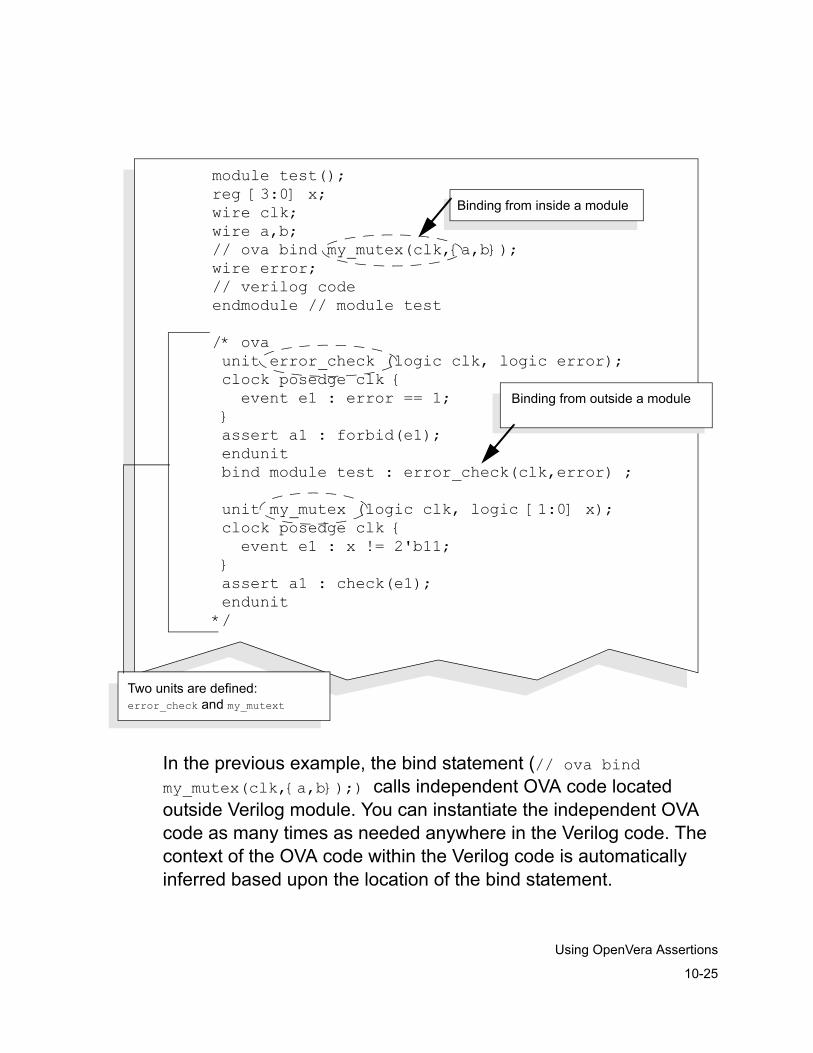
10-25
Using OpenVera Assertions
In the previous example, the bind statement (// ova bind my_mutex(clk,{a,b});) calls independent OVA code located outside Verilog module. You can instantiate the independent OVA code as many times as needed anywhere in the Verilog code. The context of the OVA code within the Verilog code is automatically inferred based upon the location of the bind statement.
module test();reg [3:0] x;wire clk;wire a,b;// ova bind my_mutex(clk,{a,b});wire error;// verilog codeendmodule // module test
/* ova unit error_check (logic clk, logic error); clock posedge clk { event e1 : error == 1; } assert a1 : forbid(e1); endunit bind module test : error_check(clk,error) ;
unit my_mutex (logic clk, logic [1:0] x); clock posedge clk { event e1 : x != 2'b11; } assert a1 : check(e1); endunit*/
Two units are defined: error_check and my_mutext
Binding from outside a module
Binding from inside a module

10-26
Using OpenVera Assertions
Template Instantiation Using the Template-Based Checker Library
You can instantiate any template-based checker from the Checker Library in your Verilog code. The context of the checker is automatically inferred based on the location of the call from within Verilog.
Note the following construct usages and limitations in Template Instantiation:
• Clocks must use edge expressions (unit-based checkers use Verilog style ports)
• You can specify the default clock in conjunction with the check_bool and forbid_bool checkers, however, it does not work with other templates or units. The following example shows a supported default clock:
//ova clock posedge clk;
Note that each sequence or boolean expression is associated with a clock. The clock determines the sampling times for variable values.
• Both for loops and nested for loops are supported, as shown below:
for (name=expr;name op1 expr;name=name op2 expr)
{for loop body}
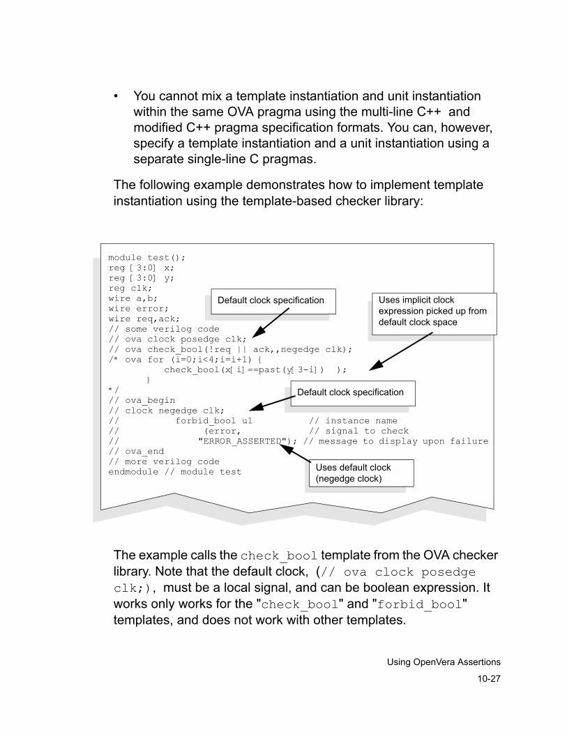
10-27
Using OpenVera Assertions
• You cannot mix a template instantiation and unit instantiation within the same OVA pragma using the multi-line C++ and modified C++ pragma specification formats. You can, however, specify a template instantiation and a unit instantiation using a separate single-line C pragmas.
The following example demonstrates how to implement template instantiation using the template-based checker library:
The example calls the check_bool template from the OVA checker library. Note that the default clock, (// ova clock posedge clk;), must be a local signal, and can be boolean expression. It works only works for the "check_bool" and "forbid_bool" templates, and does not work with other templates.
module test();reg [3:0] x;reg [3:0] y;reg clk;wire a,b;wire error;wire req,ack;// some verilog code// ova clock posedge clk;// ova check_bool(!req || ack,,negedge clk);/* ova for (i=0;i<4;i=i+1) { check_bool(x[i]==past(y[3-i]) ); }*/// ova_begin// clock negedge clk;// forbid_bool u1 // instance name// (error, // signal to check// "ERROR_ASSERTED"); // message to display upon failure// ova_end// more verilog codeendmodule // module test
Default clock specification Uses implicit clock expression picked up from default clock space
Default clock specification
Uses default clock (negedge clock)
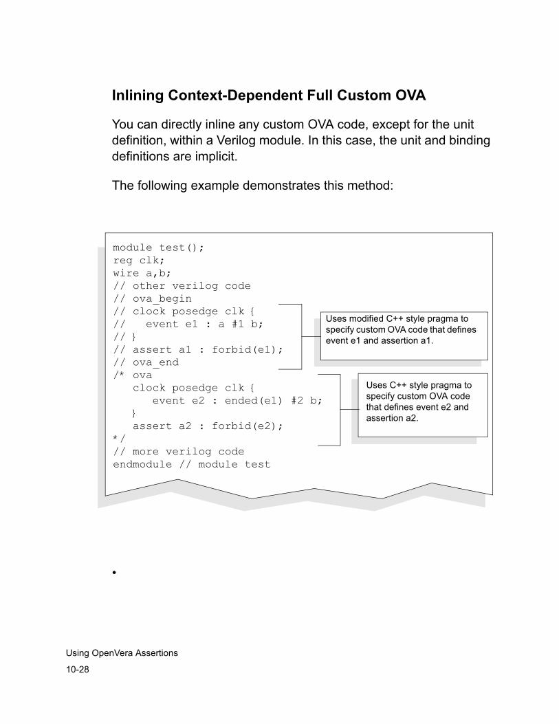
10-28
Using OpenVera Assertions
Inlining Context-Dependent Full Custom OVA
You can directly inline any custom OVA code, except for the unit definition, within a Verilog module. In this case, the unit and binding definitions are implicit.
The following example demonstrates this method:
•
module test();reg clk; wire a,b; // other verilog code// ova_begin// clock posedge clk {// event e1 : a #1 b; // } // assert a1 : forbid(e1); // ova_end/* ova clock posedge clk { event e2 : ended(e1) #2 b; } assert a2 : forbid(e2);*/ // more verilog codeendmodule // module test
Uses modified C++ style pragma to specify custom OVA code that defines event e1 and assertion a1.
Uses C++ style pragma to specify custom OVA code that defines event e2 and assertion a2.
10-29
Using OpenVera Assertions
General Inlined OVA Coding GuidelinesNote the following guidelines when coding Inlined OVA:
• Since OVA pragmas are declarative in nature, they do not need to placed within procedural code — for example, within tasks, functions, and always/initial/forever blocks.
• Cross-module References (XMRs) are not allowed to concurrently reside within a custom OVA description.
• Template instantiation will be treated as an OVA description (the XMR restriction also applies).
• Unit binding is allowed inside ‘module endmodule’, but the keyword ‘bind’ needs to be specifed in order to distinguish it from template instantiation. Unit binding (with the keyword ‘bind’) can have XMRs in its connections; however, using XMRs in connections without the bind keyword will cause a warning statement. Inlined bindings have the same requirements and limits as bindings created in an OVA source file.
• XMRs to signals are not supported except in 'bind's for inlined OVAs.
• Inlined OVA cannot be read directly by third-party simulators. You can, however, use VCS to produce output files that can be read by third-party simulators.
• Each instance must be terminated by a “;” (semi-colon).
• Both positional and named (explicit) association of actual arguments are supported. However, the two styles cannot be used simultaneously in an instance.

10-30
Using OpenVera Assertions
11-1
Using SystemVerilog Assertions
11Using SystemVerilog Assertions 1
This chapter explains the following SystemVerilog Assertions-related topics:
• Using SVA in a VHDL-Top Design
• Using SVA in a Verilog-Top Design
• Using the $hdl_xmr System Task
• Using Standard SVA Checkers
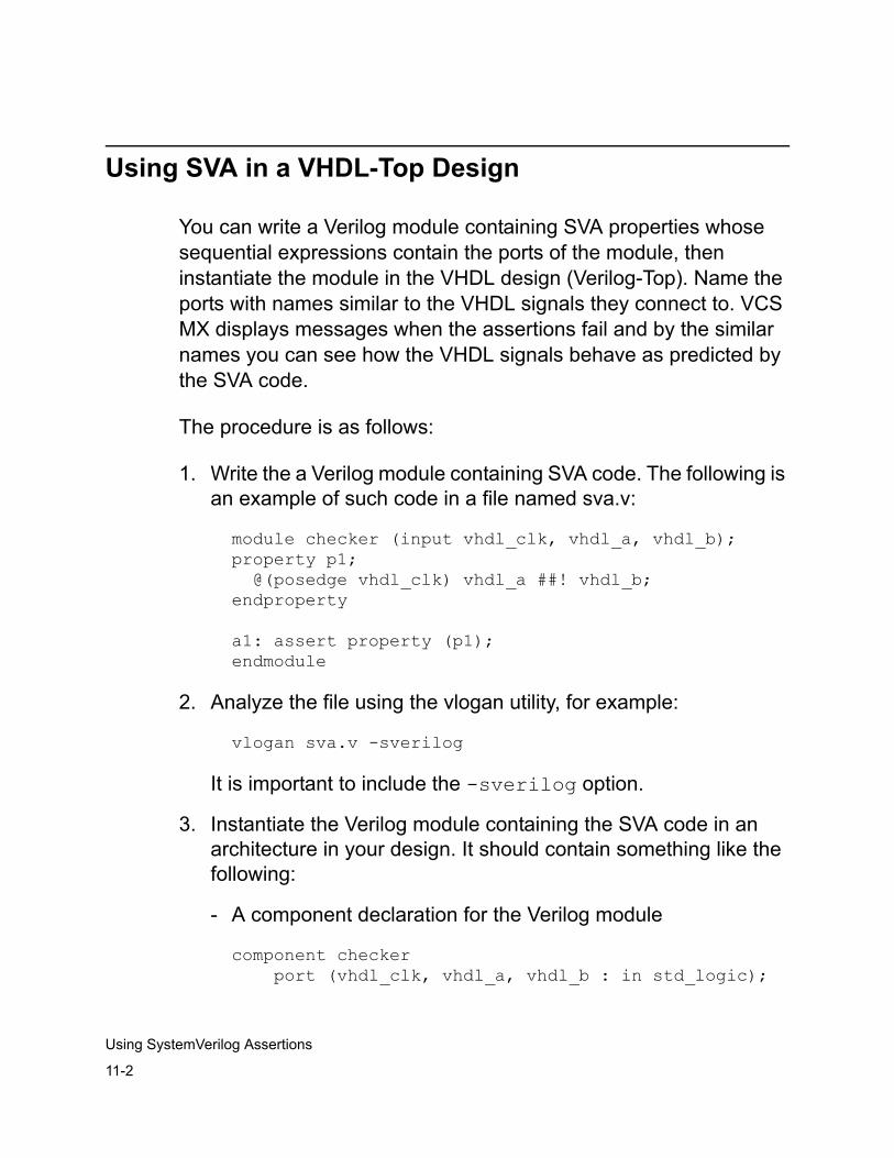
11-2
Using SystemVerilog Assertions
Using SVA in a VHDL-Top Design
You can write a Verilog module containing SVA properties whose sequential expressions contain the ports of the module, then instantiate the module in the VHDL design (Verilog-Top). Name the ports with names similar to the VHDL signals they connect to. VCS MX displays messages when the assertions fail and by the similar names you can see how the VHDL signals behave as predicted by the SVA code.
The procedure is as follows:
1. Write the a Verilog module containing SVA code. The following is an example of such code in a file named sva.v:
module checker (input vhdl_clk, vhdl_a, vhdl_b);property p1; @(posedge vhdl_clk) vhdl_a ##! vhdl_b;endproperty
a1: assert property (p1);endmodule
2. Analyze the file using the vlogan utility, for example:
vlogan sva.v -sverilog
It is important to include the -sverilog option.
3. Instantiate the Verilog module containing the SVA code in an architecture in your design. It should contain something like the following:
- A component declaration for the Verilog module
component checker port (vhdl_clk, vhdl_a, vhdl_b : in std_logic);
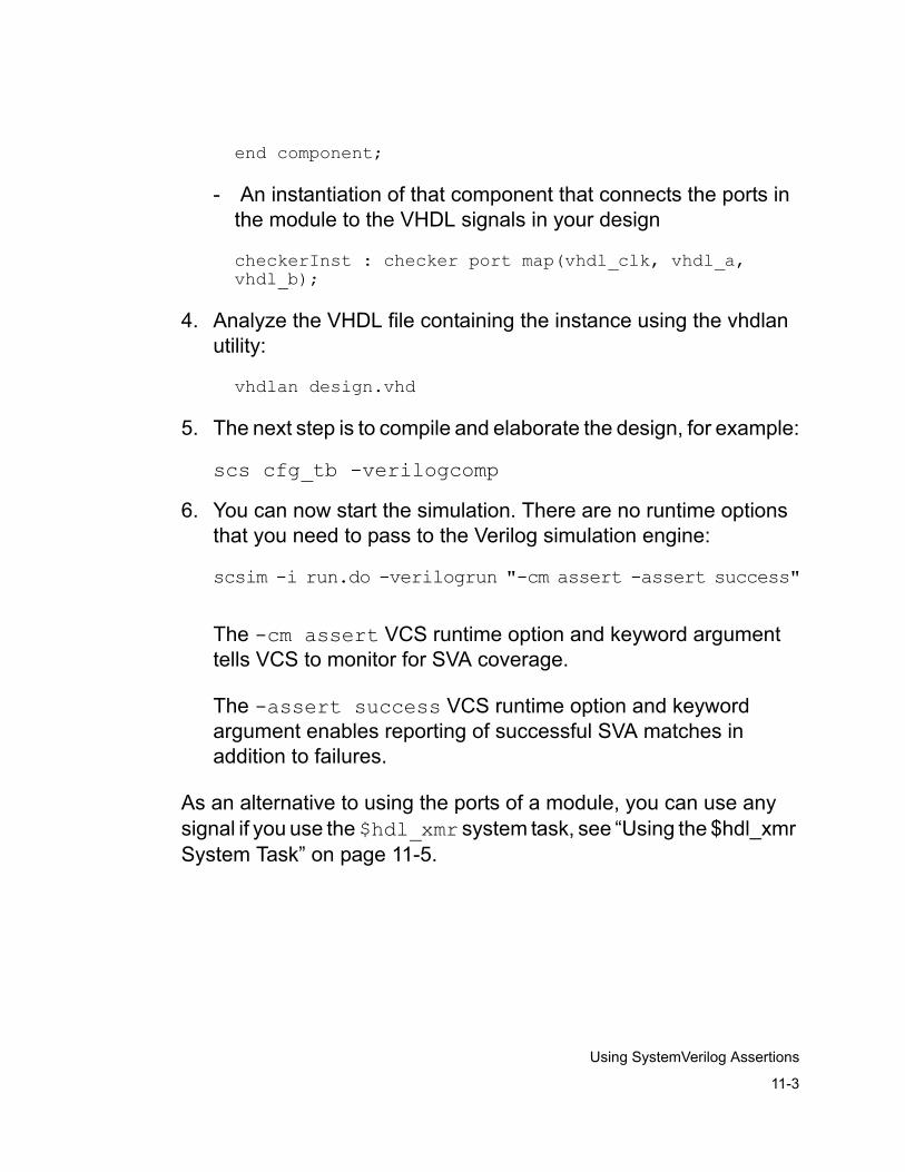
11-3
Using SystemVerilog Assertions
end component;
- An instantiation of that component that connects the ports in the module to the VHDL signals in your design
checkerInst : checker port map(vhdl_clk, vhdl_a, vhdl_b);
4. Analyze the VHDL file containing the instance using the vhdlan utility:
vhdlan design.vhd
5. The next step is to compile and elaborate the design, for example:
scs cfg_tb -verilogcomp
6. You can now start the simulation. There are no runtime options that you need to pass to the Verilog simulation engine:
scsim -i run.do -verilogrun "-cm assert -assert success"
The -cm assert VCS runtime option and keyword argument tells VCS to monitor for SVA coverage.
The -assert success VCS runtime option and keyword argument enables reporting of successful SVA matches in addition to failures.
As an alternative to using the ports of a module, you can use any signal if you use the $hdl_xmr system task, see “Using the $hdl_xmr System Task” on page 11-5.
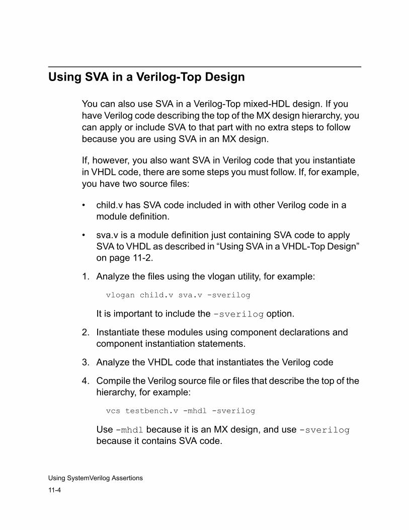
11-4
Using SystemVerilog Assertions
Using SVA in a Verilog-Top Design
You can also use SVA in a Verilog-Top mixed-HDL design. If you have Verilog code describing the top of the MX design hierarchy, you can apply or include SVA to that part with no extra steps to follow because you are using SVA in an MX design.
If, however, you also want SVA in Verilog code that you instantiate in VHDL code, there are some steps you must follow. If, for example, you have two source files:
• child.v has SVA code included in with other Verilog code in a module definition.
• sva.v is a module definition just containing SVA code to apply SVA to VHDL as described in “Using SVA in a VHDL-Top Design” on page 11-2.
1. Analyze the files using the vlogan utility, for example:
vlogan child.v sva.v -sverilog
It is important to include the -sverilog option.
2. Instantiate these modules using component declarations and component instantiation statements.
3. Analyze the VHDL code that instantiates the Verilog code
4. Compile the Verilog source file or files that describe the top of the hierarchy, for example:
vcs testbench.v -mhdl -sverilog
Use -mhdl because it is an MX design, and use -sverilog because it contains SVA code.
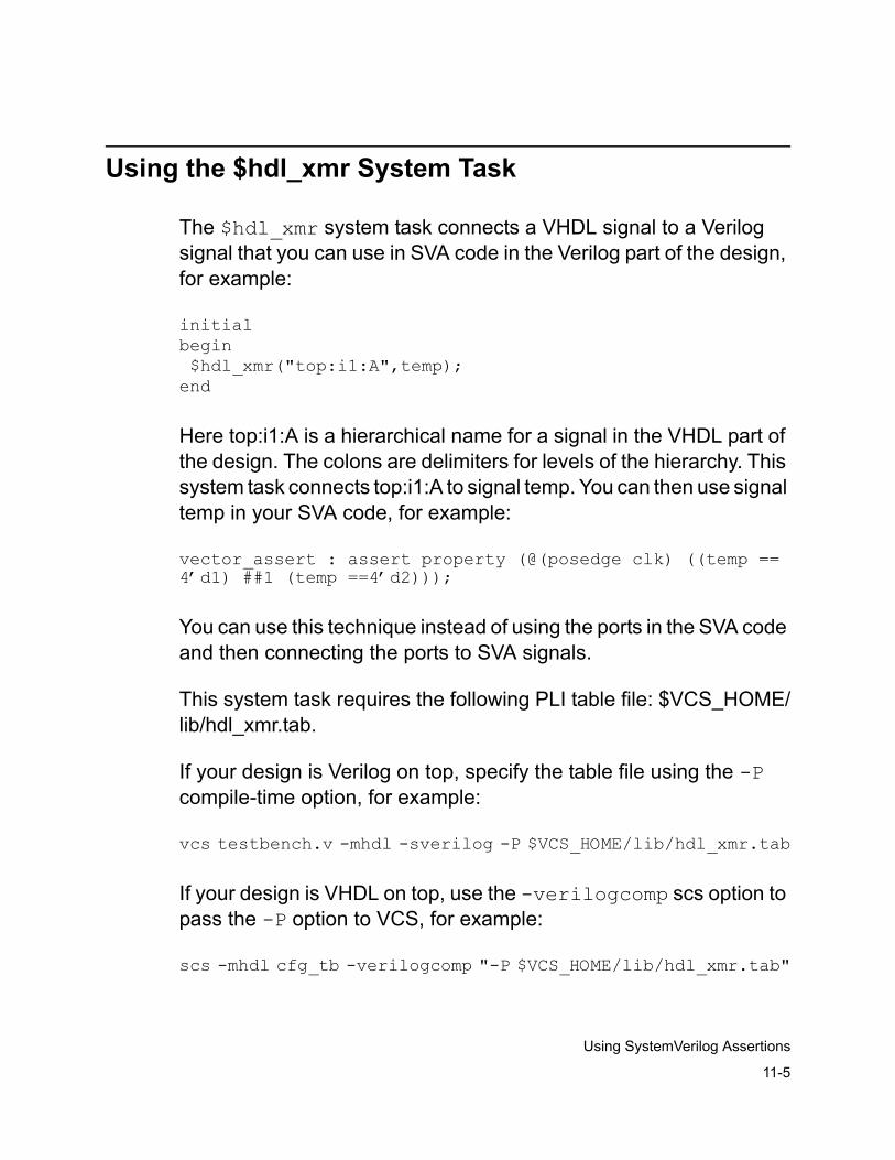
11-5
Using SystemVerilog Assertions
Using the $hdl_xmr System Task
The $hdl_xmr system task connects a VHDL signal to a Verilog signal that you can use in SVA code in the Verilog part of the design, for example:
initialbegin $hdl_xmr("top:i1:A",temp);end
Here top:i1:A is a hierarchical name for a signal in the VHDL part of the design. The colons are delimiters for levels of the hierarchy. This system task connects top:i1:A to signal temp. You can then use signal temp in your SVA code, for example:
vector_assert : assert property (@(posedge clk) ((temp == 4’d1) ##1 (temp ==4’d2)));
You can use this technique instead of using the ports in the SVA code and then connecting the ports to SVA signals.
This system task requires the following PLI table file: $VCS_HOME/lib/hdl_xmr.tab.
If your design is Verilog on top, specify the table file using the -P compile-time option, for example:
vcs testbench.v -mhdl -sverilog -P $VCS_HOME/lib/hdl_xmr.tab
If your design is VHDL on top, use the -verilogcomp scs option to pass the -P option to VCS, for example:
scs -mhdl cfg_tb -verilogcomp "-P $VCS_HOME/lib/hdl_xmr.tab"
11-6
Using SystemVerilog Assertions
Using Standard SVA Checkers
An SVA checker is SVA code provided by Synopsys that you can use in a Verilog on top MX design. Descriptions of these checkers are in the SystemVerilog Assertions (SVA) Checker Library Reference Manual. This manual contains an example of using a checker in an MX design.
You instantiate the checker components like you would any VHDL entity.
The checkers are in the $VCS_HOME/packages/sva directory.
12-1
Using the VCS MX / SystemC Co-Simulation Interface
12Using the VCS MX / SystemC Co-Simulation Interface 1
The VCS MX / SystemC Co-simulation Interface enables VCS MX and the SystemC modeling environment to work together when simulating a system described in the Verilog, VHDL, and SystemC languages.
VCS MX contains a built-in SystemC simulator that is compatible with OSCI SystemC 2.0.1. By default, when you use the interface VCS runs its own SystemC simulator. No setup is necessary.
You also have the option of installing the OSCI SystemC simulator and have VCS run it to cosimulate using the interface. See “Using a Customized SystemC Installation” on page 12-39.
12-2
Using the VCS MX / SystemC Co-Simulation Interface
With the interface you can use the most appropriate modeling language for each part of the system, and verify the correctness of the design. For example, the VCS MX / SystemC Co-simulation Interface allows you to:
• Use a SystemC module as a reference model for the VHDL or Verilog RTL design under test in your testbench.
• Verify a Verilog or VHDL netlist after synthesis with the original SystemC testbench
• Write testbenches in SystemC to check the correctness of Verilog and VHDL designs
• Import legacy VHDL or Verilog IP into a SystemC description
• Import third-party VHDL or Verilog IP into a SystemC description
• Export SystemC IP into a Verilog or VHDL environment when only a few of the design blocks are implemented in SystemC
• Use systemC to provide stimulus to your design.
The VCS MX / SystemC Co-simulation Interface creates the necessary infrastructure to co-simulate SystemC models with Verilog or VHDL models. The infrastructure consists of the required build files and any generated wrapper or stimulus code. VCS MX writes these files in subdirectories in the ./csrc directory. To use the interface, you don’t need to do anything to these files.
During co-simulation, the VCS MX / SystemC Co-simulation Interface is responsible for:
• Synchronizing the SystemC kernel and VCS MX
• Exchanging data between the two environments
12-3
Using the VCS MX / SystemC Co-Simulation Interface
The usage models for the VCS MX / SystemC Co-simulation Interface, depending on the type of cosimulation you want to perform, are the following:
• Verilog/VHDL Modules and SystemC Leaf Modules in a Verilog Design
• Verilog and VHDL Modules in a SystemC Design
• Verilog/VHDL Modules and SystemC Leaf Modules in a VHDL Design
Notes:
• There are examples of Verilog instantiated in SystemC and SystemC instantiated in Verilog in the $VCS_HOME/doc/examples/osci_dki directory.
• The interface supports the following compilers:
Linux: you can use the gnu 3.2.1 or 2.96 compilers.
Solaris: SC 6.2, gcc 2.95.2, gcc 3.2.2
HP: aCC 3.35
Usage Scenario Overview
This section contains a brief overview of the steps involved to create a simulation for each of the following design scenarios:
• Verilog designs containing SystemC and MX modules
• SystemC designs containing MX modules
• VHDL designs containing SystemC and MX modules
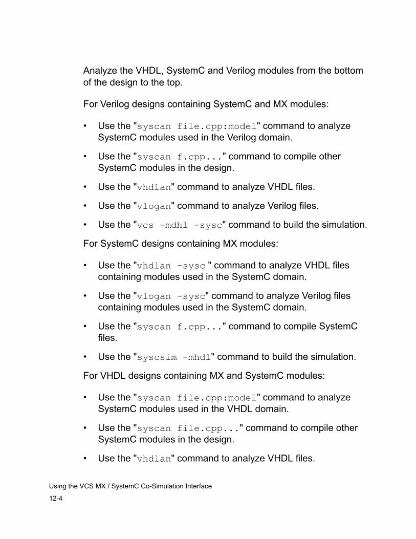
12-4
Using the VCS MX / SystemC Co-Simulation Interface
Analyze the VHDL, SystemC and Verilog modules from the bottom of the design to the top.
For Verilog designs containing SystemC and MX modules:
• Use the "syscan file.cpp:model" command to analyze SystemC modules used in the Verilog domain.
• Use the "syscan f.cpp..." command to compile other SystemC modules in the design.
• Use the "vhdlan" command to analyze VHDL files.
• Use the "vlogan" command to analyze Verilog files.
• Use the "vcs -mdhl -sysc" command to build the simulation.
For SystemC designs containing MX modules:
• Use the "vhdlan -sysc " command to analyze VHDL files containing modules used in the SystemC domain.
• Use the "vlogan -sysc" command to analyze Verilog files containing modules used in the SystemC domain.
• Use the "syscan f.cpp..." command to compile SystemC files.
• Use the "syscsim -mhdl" command to build the simulation.
For VHDL designs containing MX and SystemC modules:
• Use the "syscan file.cpp:model" command to analyze SystemC modules used in the VHDL domain.
• Use the "syscan file.cpp..." command to compile other SystemC modules in the design.
• Use the "vhdlan" command to analyze VHDL files.
12-5
Using the VCS MX / SystemC Co-Simulation Interface
• Use the "vlogan" command to analyze Verilog files.
• Use the "scs -mdhl -sysc" command to build the simulation.
Supported Port Data Types
SystemC types are restricted to the sc_clock, sc_bit, sc_bv, sc_logic, sc_lv, sc_int, sc_uint, sc_bigint, and sc_biguint data types. Native C/C++ types are restricted to the uint, uchar, ushort, int, bool, short, char, long and ulong types.
Verilog ports are restricted to bit, bit vector and signed bit vector types.
VHDL ports are restricted to bit, bit vector, standard logic, standard logic vector, signed and unsigned types.
Inout ports that cross the cosimulation boundary between SystemC and Verilog must observe the following restrictions:
• SystemC port types must be sc_inout_rv<> or sc_inout_resolved and must be connected to signals of type sc_signal_rv<> or sc_signal_resolved.
• Verilog port types must be bit_vector or bit.
• VHDL port types must be std_logic_vector or std_logic.
• You need to create a port mapping file, as described in “Using a Port Mapping File” on page 12-32, to specify the SystemC port data types as sc_lv (for a vector port) or sc_logic (for a scalar port).
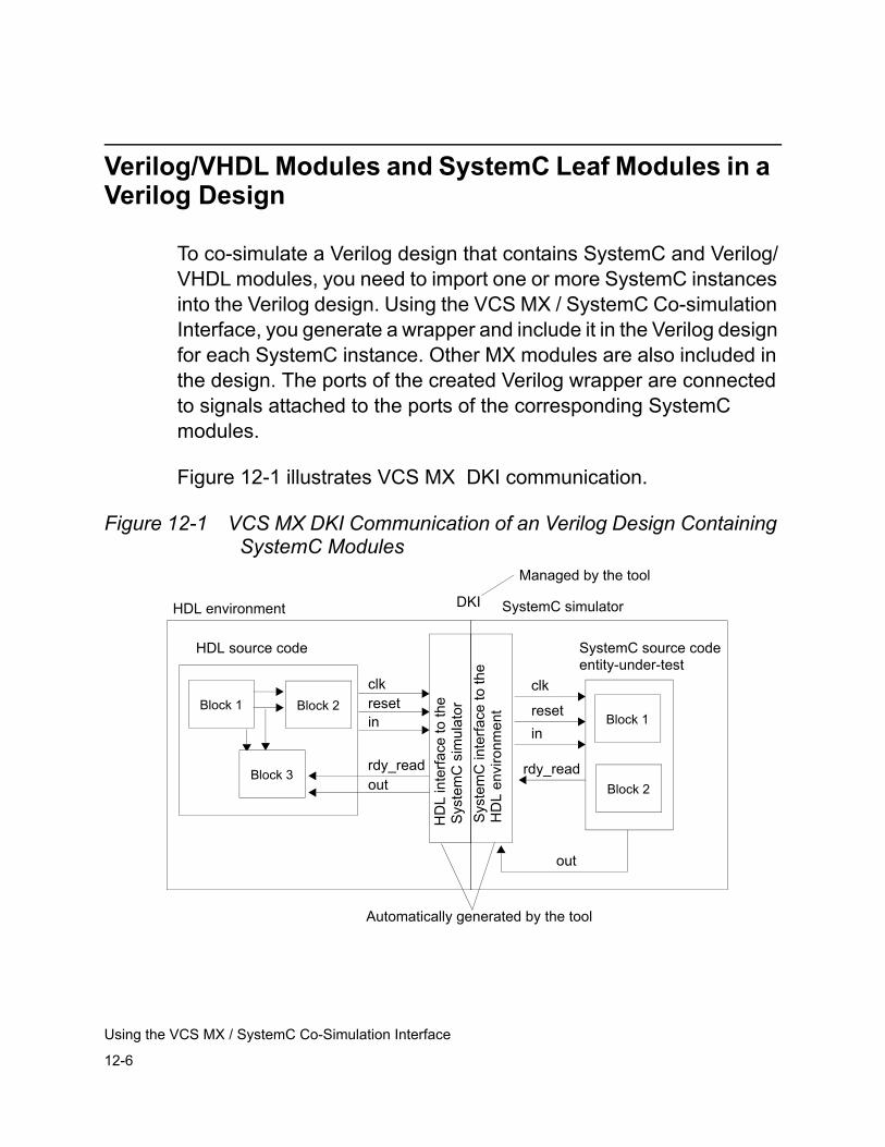
12-6
Using the VCS MX / SystemC Co-Simulation Interface
Verilog/VHDL Modules and SystemC Leaf Modules in a Verilog Design
To co-simulate a Verilog design that contains SystemC and Verilog/VHDL modules, you need to import one or more SystemC instances into the Verilog design. Using the VCS MX / SystemC Co-simulation Interface, you generate a wrapper and include it in the Verilog design for each SystemC instance. Other MX modules are also included in the design. The ports of the created Verilog wrapper are connected to signals attached to the ports of the corresponding SystemC modules.
Figure 12-1 illustrates VCS MX DKI communication.
Figure 12-1 VCS MX DKI Communication of an Verilog Design Containing SystemC Modules
DKI
clk
resetin
out
rdy_read
SystemC simulatorHDL environment
clkresetin
outrdy_read
HD
L in
terfa
ce to
the
Sys
tem
C s
imul
ator
Sys
tem
C in
terfa
ce to
the
HD
L en
viro
nmen
t
Automatically generated by the tool
Managed by the tool
Block 2
Block 1 Block 2
Block 3
Block 1
SystemC source codeentity-under-test
HDL source code
12-7
Using the VCS MX / SystemC Co-Simulation Interface
Input Files Required
To run a co-simulation with a Verilog design containing SystemC and MX instances, you need to provide the following files:
• SystemC source code
- You can directly write the entity-under-test source code or generate it with other tools.
- Any other C or C++ code for the design
• Verilog or VHDL source code (.v, .vhd, .vhdl extensions) including:
- A Verilog or VHDL top-level simulation that instantiates the interface wrapper and other Verilog/VHDL modules.These wrapper files are generated by a utility and you don’t need to do anything to these files (see “Generating the Wrapper for SystemC Modules” on page 12-8 and “Instantiating the Wrapper and Coding Style” on page 12-11).
- Any other Verilog or VHDL source files for the design
• An optional port mapping file. If you do not provide this file, the interface uses the default port mapping definition. For details of the port mapping file, see “Using a Port Mapping File” on page 12-32.
• An optional data type mapping file. If you don’t write a data type mapping file, the interface uses the default one in the VCS installation. For details of the data type mapping files, see “Using a Data Type Mapping File” on page 12-35.
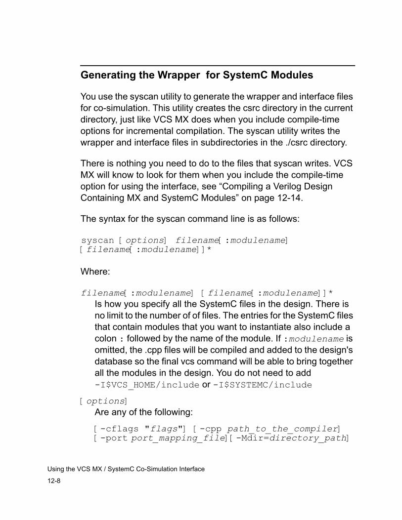
12-8
Using the VCS MX / SystemC Co-Simulation Interface
Generating the Wrapper for SystemC Modules
You use the syscan utility to generate the wrapper and interface files for co-simulation. This utility creates the csrc directory in the current directory, just like VCS MX does when you include compile-time options for incremental compilation. The syscan utility writes the wrapper and interface files in subdirectories in the ./csrc directory.
There is nothing you need to do to the files that syscan writes. VCS MX will know to look for them when you include the compile-time option for using the interface, see “Compiling a Verilog Design Containing MX and SystemC Modules” on page 12-14.
The syntax for the syscan command line is as follows:
syscan [options] filename[:modulename] [filename[:modulename]]*
Where:
filename[:modulename] [filename[:modulename]]*Is how you specify all the SystemC files in the design. There is no limit to the number of of files. The entries for the SystemC files that contain modules that you want to instantiate also include a colon : followed by the name of the module. If :modulename is omitted, the .cpp files will be compiled and added to the design's database so the final vcs command will be able to bring together all the modules in the design. You do not need to add -I$VCS_HOME/include or -I$SYSTEMC/include
[options]Are any of the following:
[-cflags "flags"] [-cpp path_to_the_compiler] [-port port_mapping_file][-Mdir=directory_path]
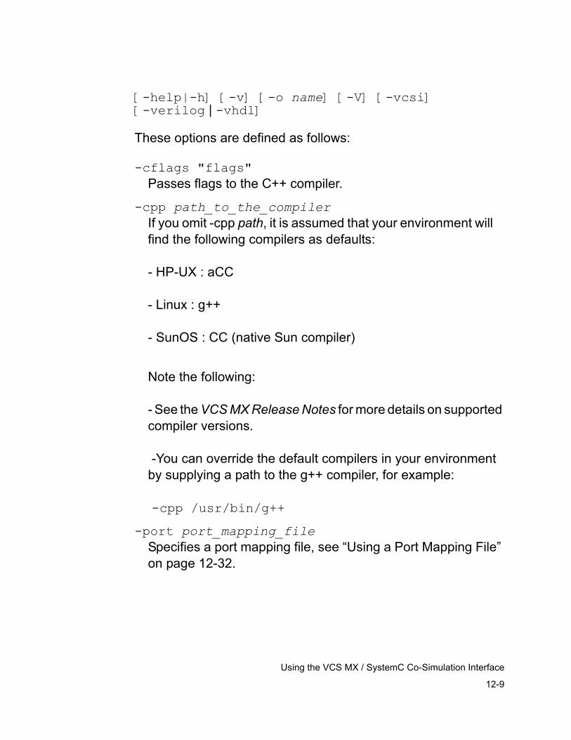
12-9
Using the VCS MX / SystemC Co-Simulation Interface
[-help|-h] [-v] [-o name] [-V] [-vcsi] [-verilog | -vhdl]
These options are defined as follows:
-cflags "flags" Passes flags to the C++ compiler.
-cpp path_to_the_compilerIf you omit -cpp path, it is assumed that your environment will find the following compilers as defaults:
- HP-UX : aCC
- Linux : g++
- SunOS : CC (native Sun compiler)
Note the following:
- See the VCS MX Release Notes for more details on supported compiler versions.
-You can override the default compilers in your environment by supplying a path to the g++ compiler, for example:
-cpp /usr/bin/g++
-port port_mapping_file Specifies a port mapping file, see “Using a Port Mapping File” on page 12-32.
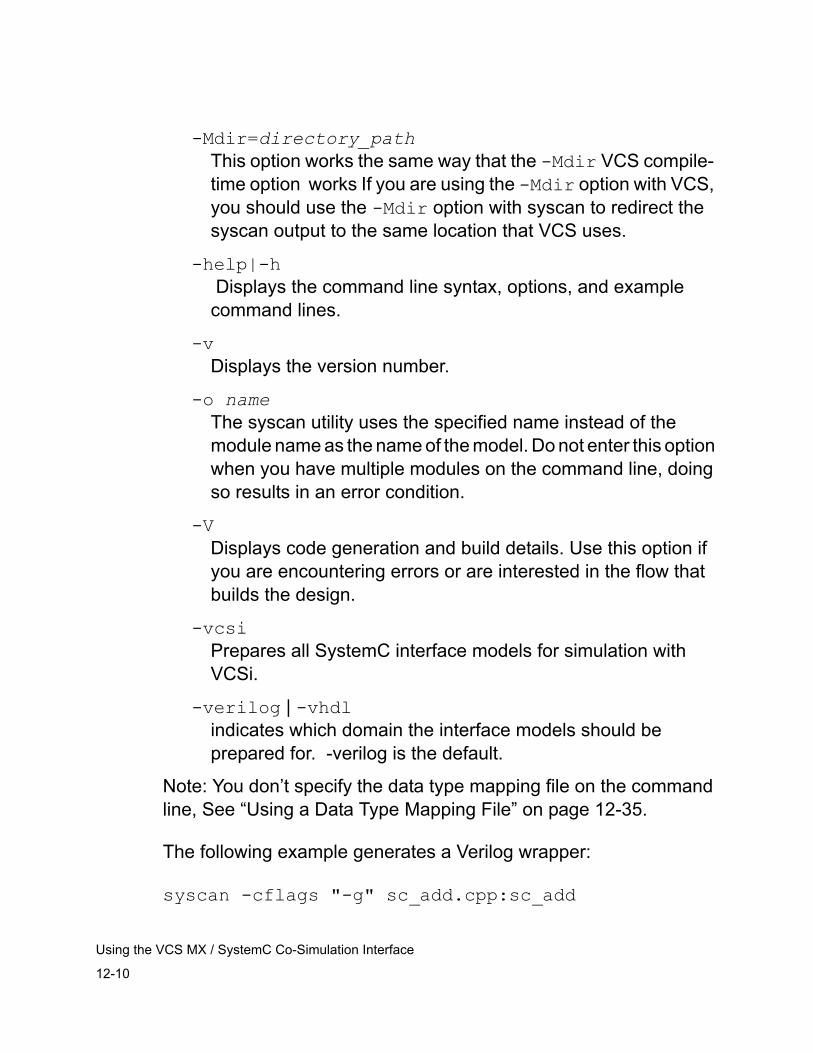
12-10
Using the VCS MX / SystemC Co-Simulation Interface
-Mdir=directory_pathThis option works the same way that the -Mdir VCS compile- time option works If you are using the -Mdir option with VCS, you should use the -Mdir option with syscan to redirect the syscan output to the same location that VCS uses.
-help|-h Displays the command line syntax, options, and example command lines.
-vDisplays the version number.
-o nameThe syscan utility uses the specified name instead of the module name as the name of the model. Do not enter this option when you have multiple modules on the command line, doing so results in an error condition.
-VDisplays code generation and build details. Use this option if you are encountering errors or are interested in the flow that builds the design.
-vcsiPrepares all SystemC interface models for simulation with VCSi.
-verilog | -vhdlindicates which domain the interface models should be prepared for. -verilog is the default.
Note: You don’t specify the data type mapping file on the command line, See “Using a Data Type Mapping File” on page 12-35.
The following example generates a Verilog wrapper:
syscan -cflags "-g" sc_add.cpp:sc_add
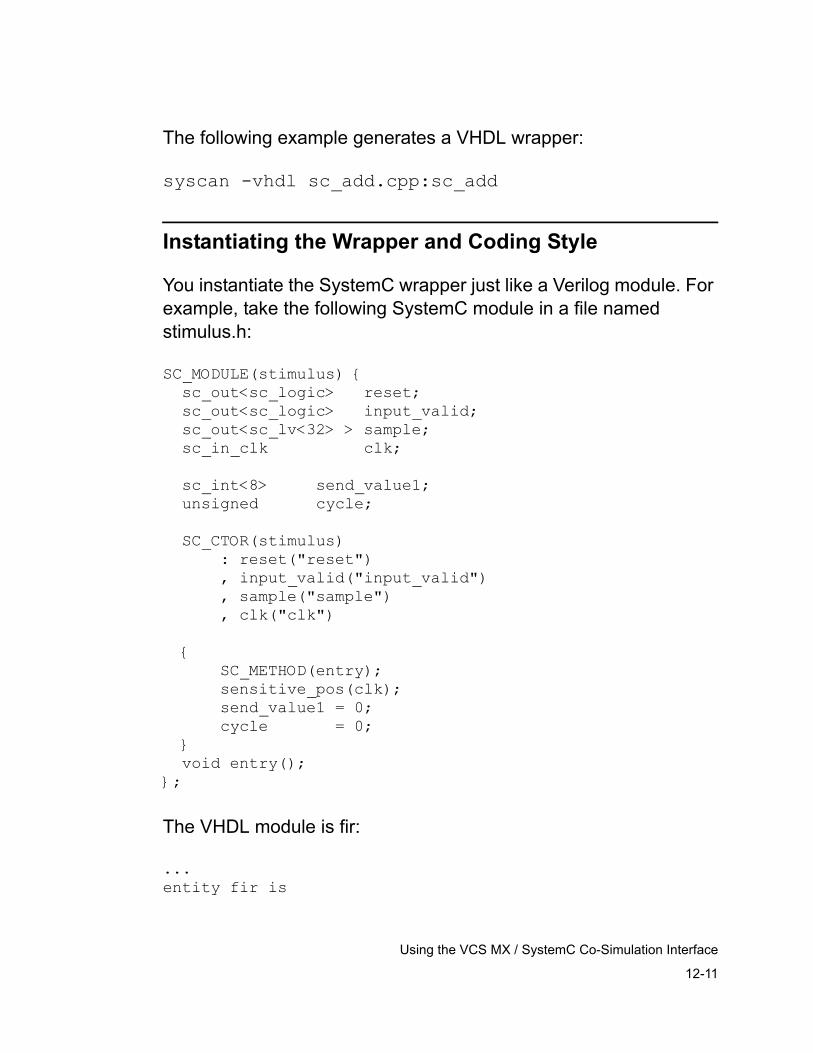
12-11
Using the VCS MX / SystemC Co-Simulation Interface
The following example generates a VHDL wrapper:
syscan -vhdl sc_add.cpp:sc_add
Instantiating the Wrapper and Coding Style
You instantiate the SystemC wrapper just like a Verilog module. For example, take the following SystemC module in a file named stimulus.h:
SC_MODULE(stimulus) { sc_out<sc_logic> reset; sc_out<sc_logic> input_valid; sc_out<sc_lv<32> > sample; sc_in_clk clk;
sc_int<8> send_value1; unsigned cycle;
SC_CTOR(stimulus) : reset("reset") , input_valid("input_valid") , sample("sample") , clk("clk")
{ SC_METHOD(entry); sensitive_pos(clk); send_value1 = 0; cycle = 0; } void entry();};
The VHDL module is fir:
...entity fir is
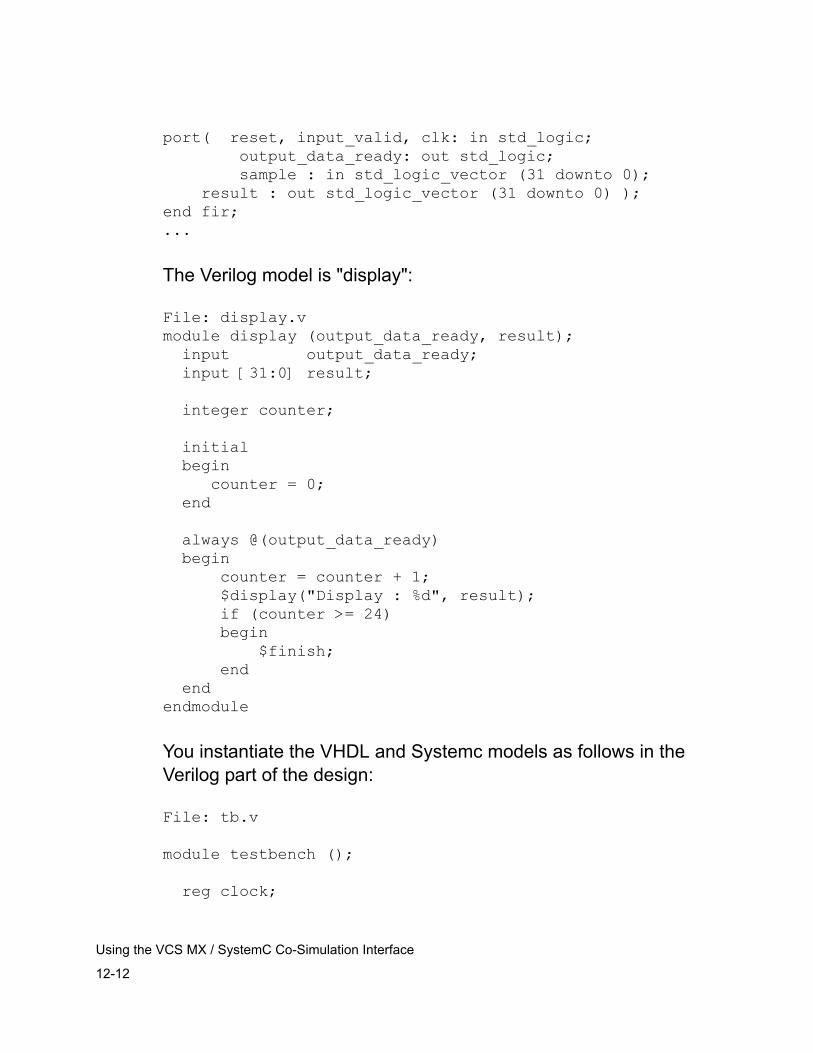
12-12
Using the VCS MX / SystemC Co-Simulation Interface
port( reset, input_valid, clk: in std_logic; output_data_ready: out std_logic; sample : in std_logic_vector (31 downto 0); result : out std_logic_vector (31 downto 0) );end fir;...
The Verilog model is "display":
File: display.vmodule display (output_data_ready, result); input output_data_ready; input [31:0] result;
integer counter;
initial begin counter = 0; end
always @(output_data_ready) begin counter = counter + 1; $display("Display : %d", result); if (counter >= 24) begin $finish; end endendmodule
You instantiate the VHDL and Systemc models as follows in the Verilog part of the design:
File: tb.v
module testbench ();
reg clock;
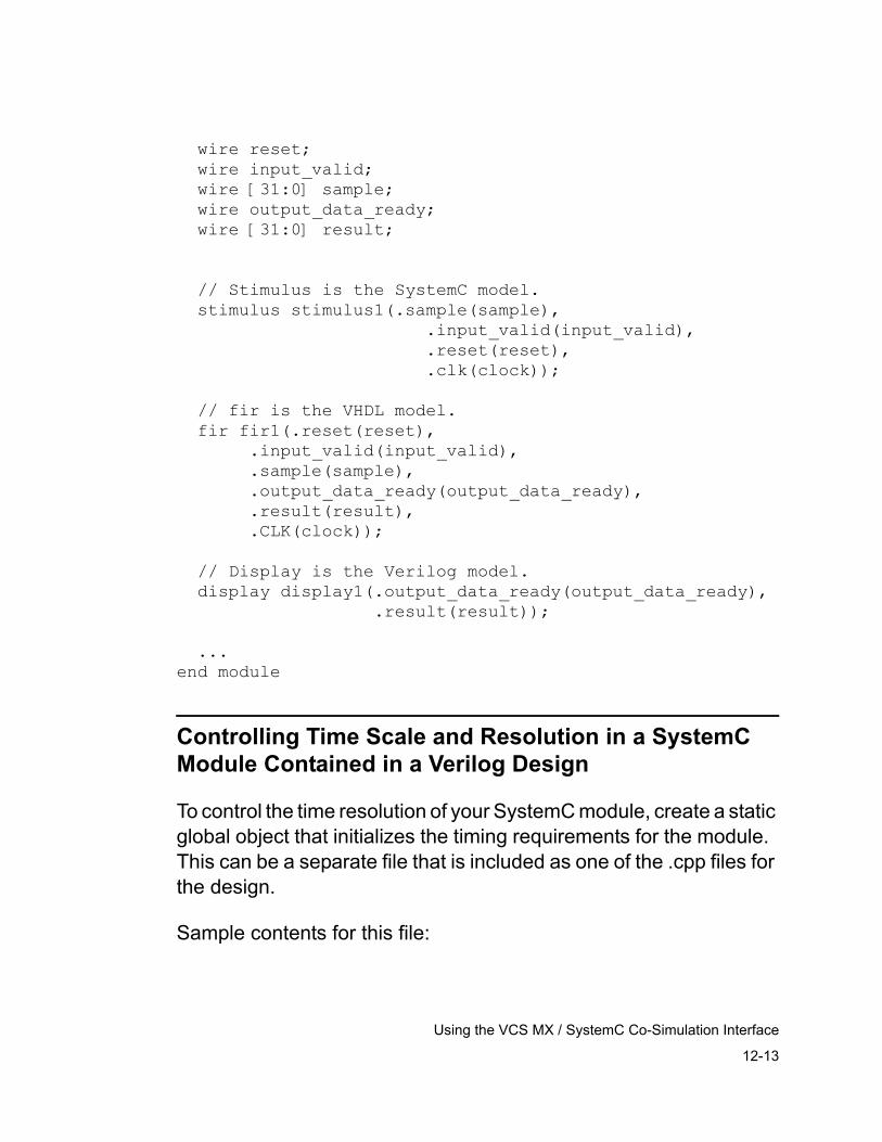
12-13
Using the VCS MX / SystemC Co-Simulation Interface
wire reset; wire input_valid; wire [31:0] sample; wire output_data_ready; wire [31:0] result;
// Stimulus is the SystemC model. stimulus stimulus1(.sample(sample), .input_valid(input_valid), .reset(reset), .clk(clock));
// fir is the VHDL model. fir fir1(.reset(reset), .input_valid(input_valid), .sample(sample), .output_data_ready(output_data_ready), .result(result), .CLK(clock));
// Display is the Verilog model. display display1(.output_data_ready(output_data_ready), .result(result));
...end module
Controlling Time Scale and Resolution in a SystemC Module Contained in a Verilog Design
To control the time resolution of your SystemC module, create a static global object that initializes the timing requirements for the module. This can be a separate file that is included as one of the .cpp files for the design.
Sample contents for this file:

12-14
Using the VCS MX / SystemC Co-Simulation Interface
#include <systemc.h>
class set_time_resolution{public: set_time_resolution() { sc_set_time_resolution(10, SC_PS); sc_set_default_time_unit(100, SC_PS); }};
static int SetTimeResolution(){ new set_time_resolution(); return 42;}
static int time_resolution_is_set = SetTimeResolution();
Analyzing Other MX Modules
Note the following when analyzing other MX Modules:
• Use vhdlan to analyze other VHDL modules.
• Use vlogan to analyze other Verilog modules.
Compiling a Verilog Design Containing MX and SystemC Modules
To compile your MX design, include the -sysc and -mhdl compile-time options, for example:
vcs -sysc -mhdl tb.v display.v
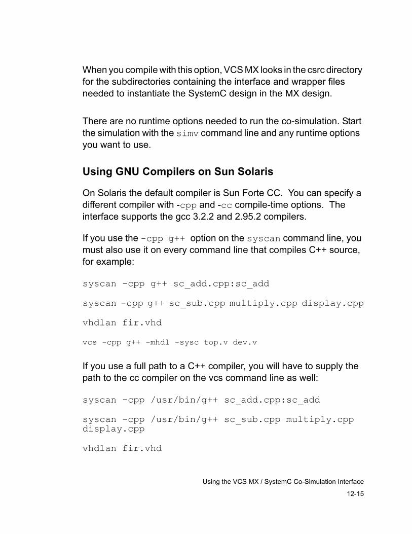
12-15
Using the VCS MX / SystemC Co-Simulation Interface
When you compile with this option, VCS MX looks in the csrc directory for the subdirectories containing the interface and wrapper files needed to instantiate the SystemC design in the MX design.
There are no runtime options needed to run the co-simulation. Start the simulation with the simv command line and any runtime options you want to use.
Using GNU Compilers on Sun Solaris
On Solaris the default compiler is Sun Forte CC. You can specify a different compiler with -cpp and -cc compile-time options. The interface supports the gcc 3.2.2 and 2.95.2 compilers.
If you use the -cpp g++ option on the syscan command line, you must also use it on every command line that compiles C++ source, for example:
syscan -cpp g++ sc_add.cpp:sc_add
syscan -cpp g++ sc_sub.cpp multiply.cpp display.cpp
vhdlan fir.vhd
vcs -cpp g++ -mhdl -sysc top.v dev.v
If you use a full path to a C++ compiler, you will have to supply the path to the cc compiler on the vcs command line as well:
syscan -cpp /usr/bin/g++ sc_add.cpp:sc_add
syscan -cpp /usr/bin/g++ sc_sub.cpp multiply.cpp display.cpp
vhdlan fir.vhd
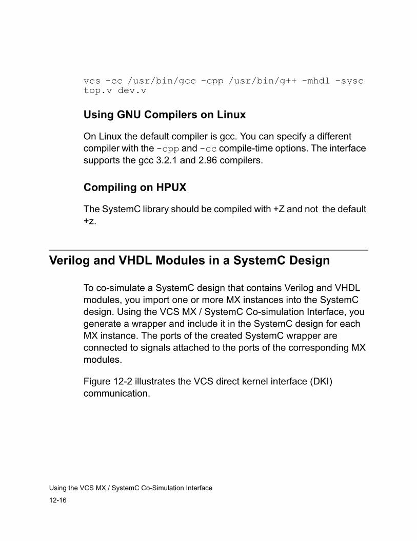
12-16
Using the VCS MX / SystemC Co-Simulation Interface
vcs -cc /usr/bin/gcc -cpp /usr/bin/g++ -mhdl -sysc top.v dev.v
Using GNU Compilers on Linux
On Linux the default compiler is gcc. You can specify a different compiler with the -cpp and -cc compile-time options. The interface supports the gcc 3.2.1 and 2.96 compilers.
Compiling on HPUX
The SystemC library should be compiled with +Z and not the default +z.
Verilog and VHDL Modules in a SystemC Design
To co-simulate a SystemC design that contains Verilog and VHDL modules, you import one or more MX instances into the SystemC design. Using the VCS MX / SystemC Co-simulation Interface, you generate a wrapper and include it in the SystemC design for each MX instance. The ports of the created SystemC wrapper are connected to signals attached to the ports of the corresponding MX modules.
Figure 12-2 illustrates the VCS direct kernel interface (DKI) communication.
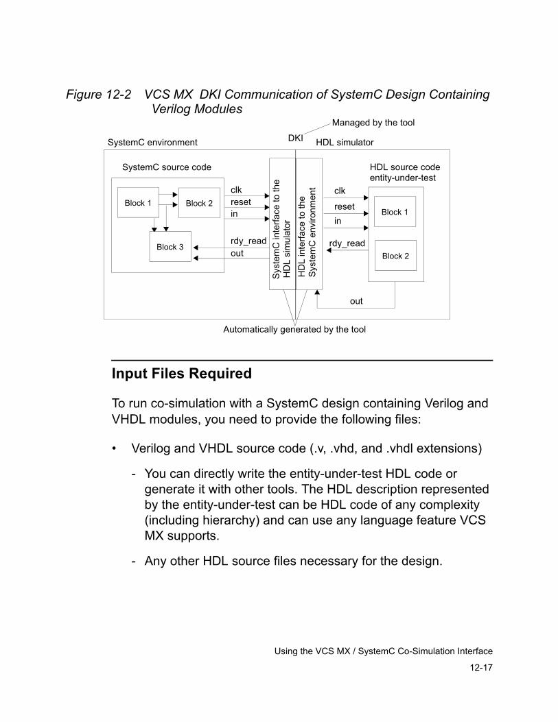
12-17
Using the VCS MX / SystemC Co-Simulation Interface
Figure 12-2 VCS MX DKI Communication of SystemC Design Containing Verilog Modules
Input Files Required
To run co-simulation with a SystemC design containing Verilog and VHDL modules, you need to provide the following files:
• Verilog and VHDL source code (.v, .vhd, and .vhdl extensions)
- You can directly write the entity-under-test HDL code or generate it with other tools. The HDL description represented by the entity-under-test can be HDL code of any complexity (including hierarchy) and can use any language feature VCS MX supports.
- Any other HDL source files necessary for the design.
DKI
clk
resetin
out
rdy_read
HDL simulatorSystemC environment
clkresetin
outrdy_read
Sys
tem
C in
terfa
ce to
the
HD
L si
mul
ator
HD
L in
terfa
ce to
the
Sys
tem
C e
nviro
nmen
t
Automatically generated by the tool
Managed by the tool
Block 2
Block 1 Block 2
Block 3
Block 1
HDL source codeentity-under-test
SystemC source code
12-18
Using the VCS MX / SystemC Co-Simulation Interface
• SystemC source code including:
- A SystemC top-level simulation (sc_main) that instantiates the interface wrappers and other SystemC modules.
- Any other SystemC source files for the design.
• An optional port mapping file. If you do not provide this file, the interface uses the default port mapping definition. For details of the port mapping file, see “Using a Port Mapping File” on page 12-32.
• An optional data type mapping file. If you don’t write a data type mapping file, the interface uses the default file in the VCS MX installation. For details of the data type mapping files, see “Using a Data Type Mapping File” on page 12-35.
Generating the Wrapper
The process for generating the wrapper depends on whether you are using Verilog or VHDL modules.
Generating the Wrapper for Verilog Modules
You use the vlogan utility with the -sysc option to generate and build the wrapper and interface files for Verilog modules for co-simulation. This utility creates the ./csrc directory in the current directory, just like VCS does when you include compile-time options for incremental compilation. The vlogan utility writes the wrapper and interface files in subdirectories in the ./csrc directory.
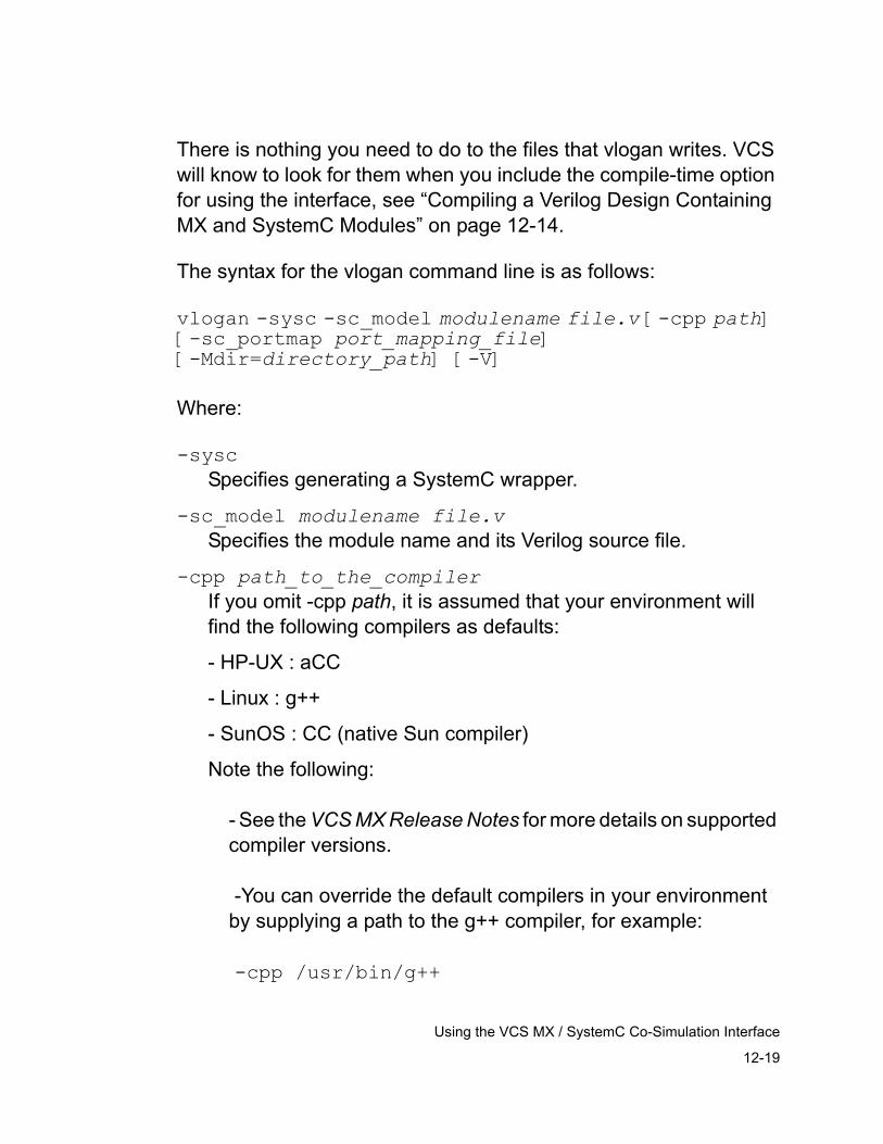
12-19
Using the VCS MX / SystemC Co-Simulation Interface
There is nothing you need to do to the files that vlogan writes. VCS will know to look for them when you include the compile-time option for using the interface, see “Compiling a Verilog Design Containing MX and SystemC Modules” on page 12-14.
The syntax for the vlogan command line is as follows:
vlogan -sysc -sc_model modulename file.v [-cpp path] [-sc_portmap port_mapping_file] [-Mdir=directory_path] [-V]
Where:
-syscSpecifies generating a SystemC wrapper.
-sc_model modulename file.vSpecifies the module name and its Verilog source file.
-cpp path_to_the_compilerIf you omit -cpp path, it is assumed that your environment will find the following compilers as defaults:
- HP-UX : aCC
- Linux : g++
- SunOS : CC (native Sun compiler)
Note the following:
- See the VCS MX Release Notes for more details on supported compiler versions.
-You can override the default compilers in your environment by supplying a path to the g++ compiler, for example:
-cpp /usr/bin/g++
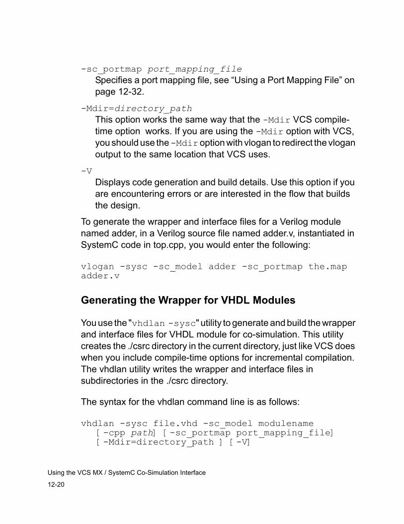
12-20
Using the VCS MX / SystemC Co-Simulation Interface
-sc_portmap port_mapping_fileSpecifies a port mapping file, see “Using a Port Mapping File” on page 12-32.
-Mdir=directory_pathThis option works the same way that the -Mdir VCS compile-time option works. If you are using the -Mdir option with VCS, you should use the -Mdir option with vlogan to redirect the vlogan output to the same location that VCS uses.
-VDisplays code generation and build details. Use this option if you are encountering errors or are interested in the flow that builds the design.
To generate the wrapper and interface files for a Verilog module named adder, in a Verilog source file named adder.v, instantiated in SystemC code in top.cpp, you would enter the following:
vlogan -sysc -sc_model adder -sc_portmap the.map adder.v
Generating the Wrapper for VHDL Modules
You use the "vhdlan -sysc" utility to generate and build the wrapper and interface files for VHDL module for co-simulation. This utility creates the ./csrc directory in the current directory, just like VCS does when you include compile-time options for incremental compilation. The vhdlan utility writes the wrapper and interface files in subdirectories in the ./csrc directory.
The syntax for the vhdlan command line is as follows:
vhdlan -sysc file.vhd -sc_model modulename [-cpp path] [-sc_portmap port_mapping_file] [-Mdir=directory_path ] [-V]
12-21
Using the VCS MX / SystemC Co-Simulation Interface
Where:
-syscSpecifies generating a SystemC wrapper.
file.vhdSpecifies the VHDL source file.
-sc_model modulename file.vSpecifies the module name and its Verilog source file.
-cpp pathIf you omit -cpp path, it is assumed that your environment will find the following compilers as defaults:
- HP-UX : aCC
- Linux : g++
- SunOS : CC (native Sun compiler)
Note the following:
- See the VCS MX Release Notes for more details on supported compiler versions.
- You can override the default compilers in your environment by supplying a path to the g++ compiler, e.g. -cpp /usr/bin/g++
-sc_portmap port_mapping_fileSpecifies a port mapping file, see “Using a Port Mapping File” on page 12-32.
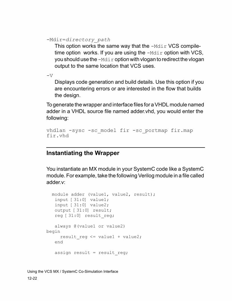
12-22
Using the VCS MX / SystemC Co-Simulation Interface
-Mdir=directory_pathThis option works the same way that the -Mdir VCS compile-time option works. If you are using the -Mdir option with VCS, you should use the -Mdir option with vlogan to redirect the vlogan output to the same location that VCS uses.
-VDisplays code generation and build details. Use this option if you are encountering errors or are interested in the flow that builds the design.
To generate the wrapper and interface files for a VHDL module named adder in a VHDL source file named adder.vhd, you would enter the following:
vhdlan -sysc -sc_model fir -sc_portmap fir.map fir.vhd
Instantiating the Wrapper
You instantiate an MX module in your SystemC code like a SystemC module. For example, take the following Verilog module in a file called adder.v:
module adder (value1, value2, result); input [31:0] value1; input [31:0] value2; output [31:0] result; reg [31:0] result_reg;
always @(value1 or value2) begin result_reg <= value1 + value2; end
assign result = result_reg;
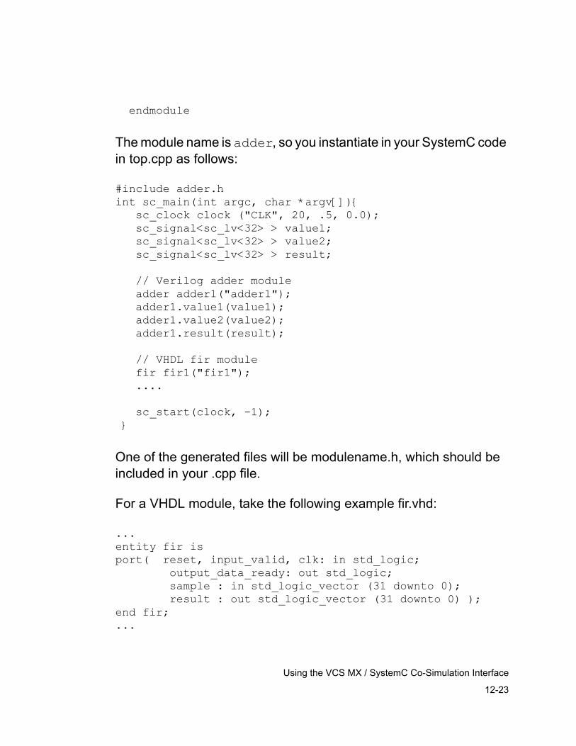
12-23
Using the VCS MX / SystemC Co-Simulation Interface
endmodule
The module name is adder, so you instantiate in your SystemC code in top.cpp as follows:
#include adder.h int sc_main(int argc, char *argv[]){ sc_clock clock ("CLK", 20, .5, 0.0); sc_signal<sc_lv<32> > value1; sc_signal<sc_lv<32> > value2; sc_signal<sc_lv<32> > result; // Verilog adder module adder adder1("adder1"); adder1.value1(value1); adder1.value2(value2); adder1.result(result);
// VHDL fir module fir fir1("fir1"); ....
sc_start(clock, -1); }
One of the generated files will be modulename.h, which should be included in your .cpp file.
For a VHDL module, take the following example fir.vhd:
...entity fir isport( reset, input_valid, clk: in std_logic; output_data_ready: out std_logic; sample : in std_logic_vector (31 downto 0); result : out std_logic_vector (31 downto 0) );end fir;...
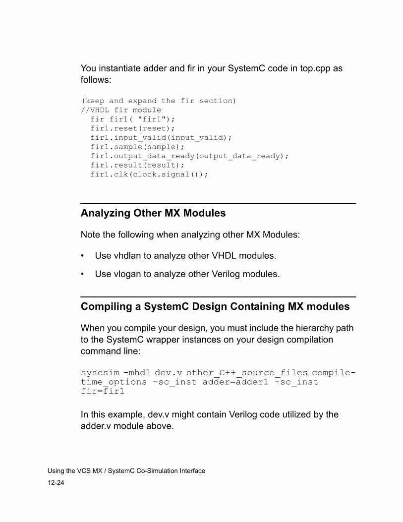
12-24
Using the VCS MX / SystemC Co-Simulation Interface
You instantiate adder and fir in your SystemC code in top.cpp as follows:
(keep and expand the fir section)//VHDL fir module fir fir1( "fir1"); fir1.reset(reset); fir1.input_valid(input_valid); fir1.sample(sample); fir1.output_data_ready(output_data_ready); fir1.result(result); fir1.clk(clock.signal());
Analyzing Other MX Modules
Note the following when analyzing other MX Modules:
• Use vhdlan to analyze other VHDL modules.
• Use vlogan to analyze other Verilog modules.
Compiling a SystemC Design Containing MX modules
When you compile your design, you must include the hierarchy path to the SystemC wrapper instances on your design compilation command line:
syscsim -mhdl dev.v other_C++_source_files compile-time_options -sc_inst adder=adder1 -sc_inst fir=fir1
In this example, dev.v might contain Verilog code utilized by the adder.v module above.
12-25
Using the VCS MX / SystemC Co-Simulation Interface
When you compile with this option, VCS MX looks in the ./csrc directory for the subdirectories containing the interface and wrapper files needed to connect the Verilog and SystemC parts of the design.
There are no runtime options for SystemC cosimulation. Start the simulation with a simv command line and any runtime options that you want to use.
Specifying Run-Time Options to the SystemC Simulation
You start a simulation with the simv command line. You enter SystemC parameters or arguments (analogous to Verilog runtime options), to control the simulation of the SystemC part of the design, on the simv command line, for example:
simv scarg1 scarg2
If you also want to enter a VHDL runtime option, to control the simulation of the VHDL part of the design, you can do so by preceding it with the -vhdlrun option on the simv command line, for example:
simv scarg1 -vhdlrun -verb
If you want to enter both Verilog and VHDL run-time options to control the simulationof the Verilog and VHDL parts of the design, you can use the -verilogrun and -vhdlrun options, for example:
simv scarg1 -verilogrun -q -vhdlrun "-prof prof.html"
12-26
Using the VCS MX / SystemC Co-Simulation Interface
Using GNU Compilers on SUN Solaris
On Solaris the default compiler is Sun Forte CC. You can specify a different compiler with -cpp and -cc compile-time options. The interface supports the gcc 3.2.2 and 2.95.2 compilers.
If you use the -cpp g++ option on the interface analysis command line, you must also use it on every command line that compiles C++ source:
vhdlan -sysc -cpp g++ fir.vhd -sc_model fir
vlogan -sysc -cpp g++ display.v -sc_model display
syscsim -cpp g++ -mhdl -sysc main.cpp a.cpp -sc_inst display=display1 -sc_inst fir=fir1
If you use a full path to a C++ compiler, you will have to supply the path to the cc compiler on the command line that builds the simulation as well:
vhdlan -sysc -cpp /usr/bin/g++ fir.vhd -sc_model fir
vlogan -sysc -cpp /usr/bin/g++ display.v -sc_model display
syscsim -cc /usr/bin/gcc -cpp /usr/bin/g++ -mhdl -sysc main.cpp a.cpptop.v dev.v
12-27
Using the VCS MX / SystemC Co-Simulation Interface
Using GNU Compilers on Linux
On Linux the default compiler is gcc. You can specify a different compiler with the -cpp and -cc compile-time options. The interface supports the gcc 3.2.1 and 2.96 compilers.
Compiling on HPUX
The SystemC library should be compiled with +Z and not the default +z.
Verilog/VHDL Modules and SystemC Leaf Modules in a VHDL Design
To co-simulate a VHDL design that contains SystemC leaf modules and Verilog/VHDL modules, you import one or more SystemC instances into the VHDL design. Using the VCS MX / SystemC Co-simulation Interface, you generate a wrapper and include it in the VHDL design for each SystemC instance.
Other MX modules are also included in the design. The ports of the created VHDL wrapper are connected to signals attached to the ports of the corresponding SystemC modules.
Figure 12-1 on page 12-6 illustrates VCS MX communication.
Required Input Files
To run co-simulation with a VHDL design containing SystemC, Verilog and VHDL modules, you need to provide the following files:
12-28
Using the VCS MX / SystemC Co-Simulation Interface
• SystemC source code
- You can directly write the entity-under-test source code or generate it with other tools.
- Any other C or C++ code for the design.
• HDL source code (.v, .vhd or .vhdl extension) including:
- A Verilog or VHDL module definition that instantiates the interface wrapper and other MX modules. These wrapper files are generated by a utility and you don’ t need to do anything to these files (see “Generating the Wrapper for SystemC Modules” on page 12-28
• Any other VHDL source files for the design
• An optional port mapping file. If you do not provide this file, the interface uses the default port mapping definition. For details of the port mapping file, see “Using a Port Mapping File” on page 12-32.
• An optional data type mapping file. If you don’t write a data type mapping file, the interface uses the default one in the VCS installation. For details of the data type mapping files, see “Using a Data Type Mapping File” on page 12-35.
Generating the Wrapper for SystemC Modules
You use the syscan utility to generate the wrapper and interface files for cosimulation. This utility creates the csrc directory in the current directory, just like VCS does when you include compile-time options for incremental compilation. The syscan utility writes the wrapper and interface files in subdirectories in the ./csrc directory.
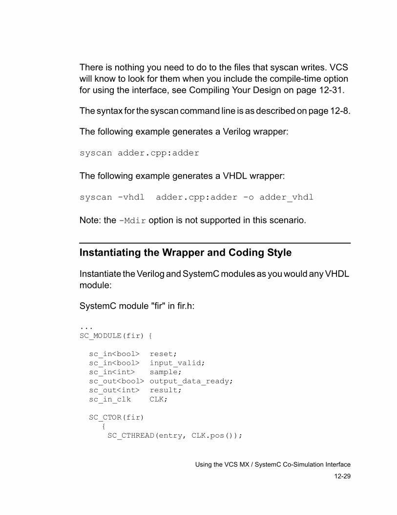
12-29
Using the VCS MX / SystemC Co-Simulation Interface
There is nothing you need to do to the files that syscan writes. VCS will know to look for them when you include the compile-time option for using the interface, see Compiling Your Design on page 12-31.
The syntax for the syscan command line is as described on page 12-8.
The following example generates a Verilog wrapper:
syscan adder.cpp:adder
The following example generates a VHDL wrapper:
syscan -vhdl adder.cpp:adder -o adder_vhdl
Note: the -Mdir option is not supported in this scenario.
Instantiating the Wrapper and Coding Style
Instantiate the Verilog and SystemC modules as you would any VHDL module:
SystemC module "fir" in fir.h:
...SC_MODULE(fir) {
sc_in<bool> reset; sc_in<bool> input_valid; sc_in<int> sample; sc_out<bool> output_data_ready; sc_out<int> result; sc_in_clk CLK;
SC_CTOR(fir) { SC_CTHREAD(entry, CLK.pos());
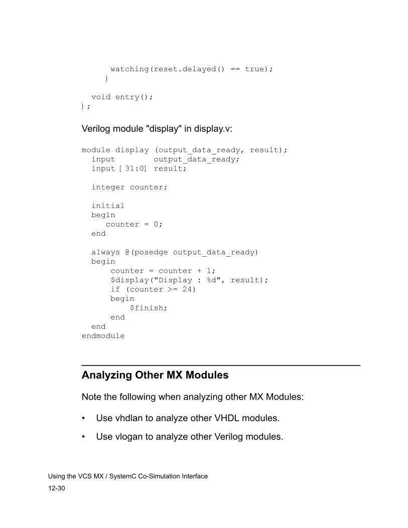
12-30
Using the VCS MX / SystemC Co-Simulation Interface
watching(reset.delayed() == true); }
void entry();};
Verilog module "display" in display.v:
module display (output_data_ready, result); input output_data_ready; input [31:0] result;
integer counter;
initial begin counter = 0; end
always @(posedge output_data_ready) begin counter = counter + 1; $display("Display : %d", result); if (counter >= 24) begin $finish; end endendmodule
Analyzing Other MX Modules
Note the following when analyzing other MX Modules:
• Use vhdlan to analyze other VHDL modules.
• Use vlogan to analyze other Verilog modules.
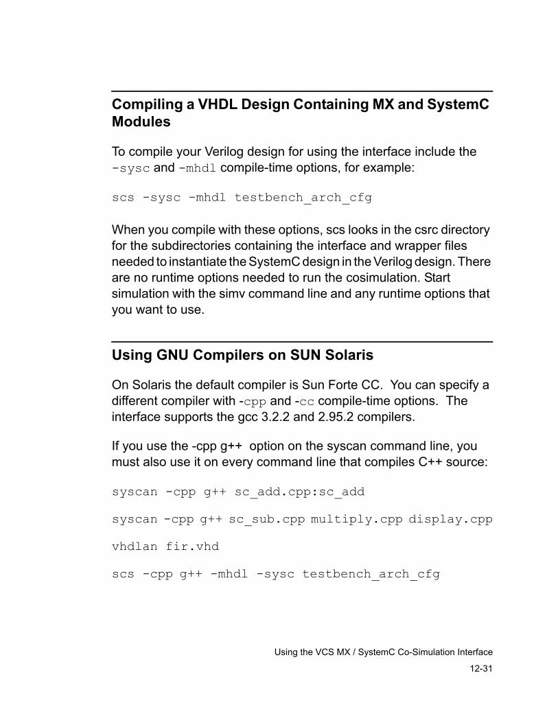
12-31
Using the VCS MX / SystemC Co-Simulation Interface
Compiling a VHDL Design Containing MX and SystemC Modules
To compile your Verilog design for using the interface include the -sysc and -mhdl compile-time options, for example:
scs -sysc -mhdl testbench_arch_cfg
When you compile with these options, scs looks in the csrc directory for the subdirectories containing the interface and wrapper files needed to instantiate the SystemC design in the Verilog design. There are no runtime options needed to run the cosimulation. Start simulation with the simv command line and any runtime options that you want to use.
Using GNU Compilers on SUN Solaris
On Solaris the default compiler is Sun Forte CC. You can specify a different compiler with -cpp and -cc compile-time options. The interface supports the gcc 3.2.2 and 2.95.2 compilers.
If you use the -cpp g++ option on the syscan command line, you must also use it on every command line that compiles C++ source:
syscan -cpp g++ sc_add.cpp:sc_add
syscan -cpp g++ sc_sub.cpp multiply.cpp display.cpp
vhdlan fir.vhd
scs -cpp g++ -mhdl -sysc testbench_arch_cfg
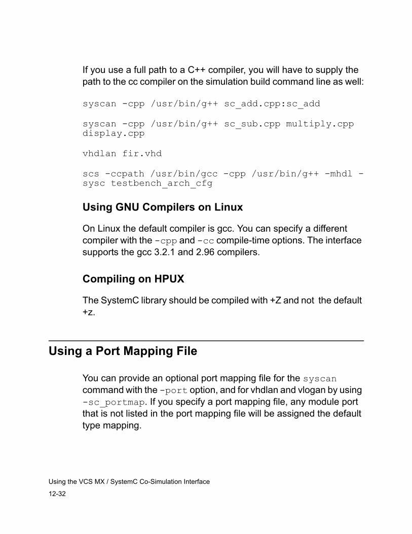
12-32
Using the VCS MX / SystemC Co-Simulation Interface
If you use a full path to a C++ compiler, you will have to supply the path to the cc compiler on the simulation build command line as well:
syscan -cpp /usr/bin/g++ sc_add.cpp:sc_add
syscan -cpp /usr/bin/g++ sc_sub.cpp multiply.cpp display.cpp
vhdlan fir.vhd
scs -ccpath /usr/bin/gcc -cpp /usr/bin/g++ -mhdl -sysc testbench_arch_cfg
Using GNU Compilers on Linux
On Linux the default compiler is gcc. You can specify a different compiler with the -cpp and -cc compile-time options. The interface supports the gcc 3.2.1 and 2.96 compilers.
Compiling on HPUX
The SystemC library should be compiled with +Z and not the default +z.
Using a Port Mapping File
You can provide an optional port mapping file for the syscan command with the -port option, and for vhdlan and vlogan by using -sc_portmap. If you specify a port mapping file, any module port that is not listed in the port mapping file will be assigned the default type mapping.
12-33
Using the VCS MX / SystemC Co-Simulation Interface
A SystemC port has a corresponding Verilog or VHDL port in the wrapper for instantiation. The syscan utility either uses the default method for determining the type of the HDL port it writes in the wrapper or uses the entry for the port in the port mapping file.
A port mapping file is an ASCII text file.Each line defines a port in the SystemC module, using the format in Example x and y. A line beginning with a pound sign (#) is a comment.
A port definition line begins with a port name, which must be the same name as that of a port in the HDL module or entity. Specify the number of bits, the HDL port type, and the SystemC port type on the same line, separated by white space. You can specify the port definition lines in any order. You must, however, provide the port definition parameters in this order: port name, bits, HDL type, and SystemC type.
The valid Verilog port types, which are case-insensitive, are as follows:
• bit — specifies a scalar (single bit) Verilog port.
• bit_vector — specifies a vector (multi-bit) unsigned Verilog port (bitvector is a valid alternative).
• signed — specifies a Verilog port that is also a reg or a net declared with the signed keyword and propagates a signed value.
The valid VHDL port types, which are case-insensitive, are:
• bit
• bitvector
• std_logic
• std_logic_vector
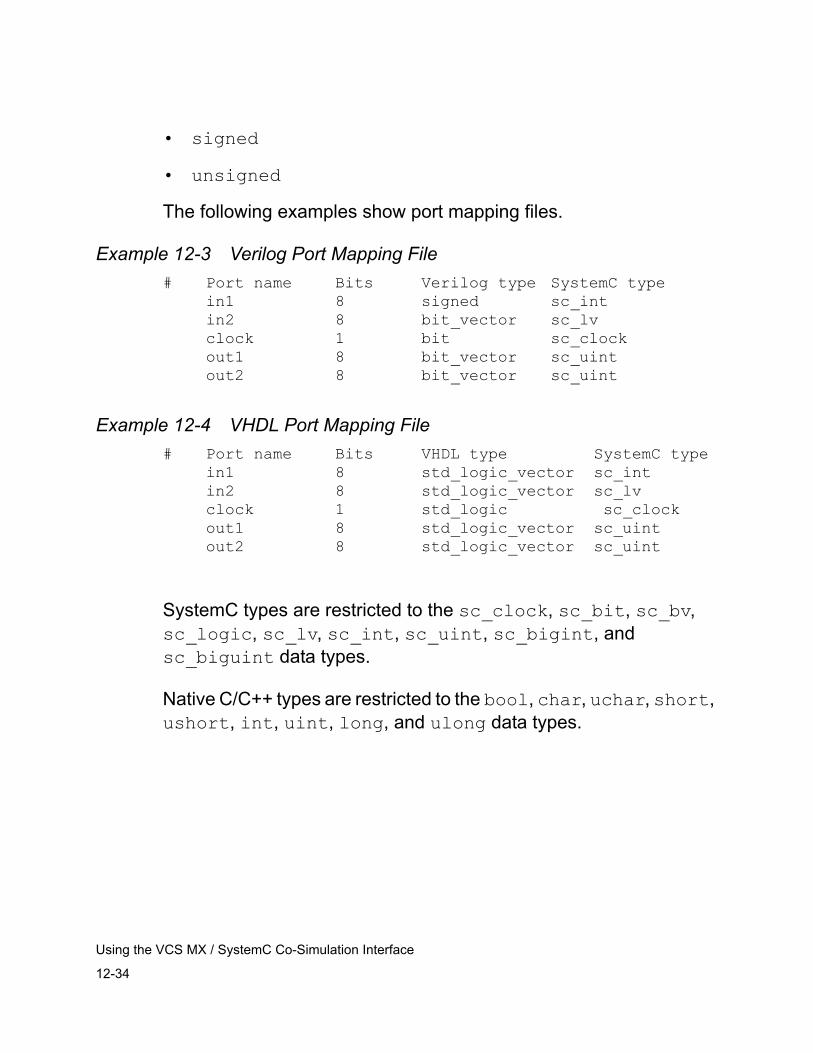
12-34
Using the VCS MX / SystemC Co-Simulation Interface
• signed
• unsigned
The following examples show port mapping files.
Example 12-3 Verilog Port Mapping File# Port name Bits Verilog type SystemC type
in1 8 signed sc_intin2 8 bit_vector sc_lvclock 1 bit sc_clockout1 8 bit_vector sc_uintout2 8 bit_vector sc_uint
Example 12-4 VHDL Port Mapping File# Port name Bits VHDL type SystemC type
in1 8 std_logic_vector sc_intin2 8 std_logic_vector sc_lvclock 1 std_logic sc_clockout1 8 std_logic_vector sc_uintout2 8 std_logic_vector sc_uint
SystemC types are restricted to the sc_clock, sc_bit, sc_bv, sc_logic, sc_lv, sc_int, sc_uint, sc_bigint, and sc_biguint data types.
Native C/C++ types are restricted to the bool, char, uchar, short, ushort, int, uint, long, and ulong data types.
12-35
Using the VCS MX / SystemC Co-Simulation Interface
Using a Data Type Mapping File
When running a VCS MX / SystemC simulation, the interface propagates data through the module ports from one language domain to another. This can require the interface to translate data from one data type representation to another. This translation is called mapping and is controlled by data type mapping files.
The datatype mapping mechanism is similar to that used for port mapping (see “Using a Port Mapping File” on page 12-32), but is more economical and requires less effort to create and maintain. Because the datatype mapping is independent of the ports, you can create one or more default mappings for a particular type that will be used for all ports, rather than having to create a port map for every port of each new HDL wrapper model.
Data type mapping files map types, so that ALL ports of that type on ALL instances will now be assigned the specified mapping.
The data type mapping file is named cosim_defaults.map. The interface looks for and reads the data mapping file in the following places and in the following order:
1. In $VCS_HOME/include/cosim
2. In your $HOME/.synopsys_ccss directory
3. In the current directory.
An entry in a later file overrules an entry in an earlier file.
Each entry for a SystemC type has the following:
1. It begins with the keyword Verilog or VHDL.
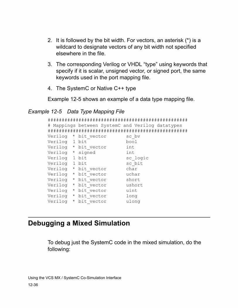
12-36
Using the VCS MX / SystemC Co-Simulation Interface
2. It is followed by the bit width. For vectors, an asterisk (*) is a wildcard to designate vectors of any bit width not specified elsewhere in the file.
3. The corresponding Verilog or VHDL “type” using keywords that specify if it is scalar, unsigned vector, or signed port, the same keywords used in the port mapping file.
4. The SystemC or Native C++ type
Example 12-5 shows an example of a data type mapping file.
Example 12-5 Data Type Mapping File################################################### Mappings between SystemC and Verilog datatypes##################################################Verilog * bit_vector sc_bvVerilog 1 bit boolVerilog * bit_vector intVerilog * signed intVerilog 1 bit sc_logicVerilog 1 bit sc_bitVerilog * bit_vector charVerilog * bit_vector ucharVerilog * bit_vector shortVerilog * bit_vector ushortVerilog * bit_vector uintVerilog * bit_vector longVerilog * bit_vector ulong
Debugging a Mixed Simulation
To debug just the SystemC code in the mixed simulation, do the following:
12-37
Using the VCS MX / SystemC Co-Simulation Interface
1. Run syscan with the -cflags "-g" option to build the SystemC source code for debugging.
2. Start the C++ debugger on the simv executable file.
If you are using the Sun Forte compiler:
dbx ./simv
If you are using the Gnu compiler on Solaris or Linux:
Run both syscan and VCS with the -cpp path option
gdb ./simv
If you are using the aCC compiler on the HP platform, you can use either the gdb or wdb debugger:
gdb ./simv wdb ./simv
You can now set and stop at breakpoints in your SystemC code.
To also debug the Verilog/VHDL portions of your design, follow the debug instructions in the VCS MX User's Guide under "Debugging and Post-Processing" for mixed designs to enable debugging in the VHDL and/or Verilog modules. With either the VCS or VCS MX debugger running, find the simv/scsim executable process id:
% ps -e | grep simv (or scsim)12216 pts/1 0:00 simv
Launch your SystemC debugger using the process ID to connect to the running simulations, for example:
12-38
Using the VCS MX / SystemC Co-Simulation Interface
% gdb ./simv 12216
Using the Built-in SystemC Simulator
VCS MX contains a built-in SystemC which it uses by default. No setup is necessary. Using this simulator does not require setting an environment variable (in earlier releases, the interface required the SYSTEMC environment variable).
Compatibility with OSCI SystemC 2.0.1
The built-in SystemC simulator is binary compatible to the OSCISystemC 2.0.1 simulator. That means that you can link into a simvexecutable objects files (*.{o,a,so}) compiled with the OSCI SystemC2.0.1 simulator.
Supported Compilers
The following compilers are supported:
• Linux: gcc 2.96 and gcc 3.2.1
• Solaris: SC 6.2, gcc 2.95.2, gcc 3.2.2
• HP: aCC 3.35
Compiling Source Files
If you need to compile source files that include systemc.h in your own environment and not with the syscan script, then addcompiler flag -I$VCS_HOME/include/systemc.
12-39
Using the VCS MX / SystemC Co-Simulation Interface
Using a Customized SystemC Installation
Important:This feature is not available in VCS 7.2 beta.
You can install the OSCI SystemC simulator and tell VCS MX to use it for Verilog/VHDL/SystemC cosimulation. To do so you set the SYSTEMC_OVVERRIDE environment variable to the directory where you installed it, for example:
setenv SYSTEMC_OVERRIDE /net/user/systemc-2.0.1
The OSCI SystemC simulator installation must have the usual OSCI structure of $SYSTEMC_OVERRIDE/include and $SYSTEMC_OVERRIDE/lib-<arch>/libsystemc.a.
The installation must contain the patches required for the cosimulation interface.
Compatibility with OSCI SystemC 2.0.1
The built-in SystemC simulator is binary compatible to the OSCI SystemC 2.0.1 simulator. That means that you can link into a simv executable objects files (*.{o,a,so}) compiled with the OSCI SystemC 2.0.1 simulator.
Supported Compilers
The following compilers are supported:
Linux: gcc 2.96 and gcc 3.2.1
Solaris: SC 6.2, gcc 2.95.2, gcc 3.2.2
HP: aCC 3.35
12-40
Using the VCS MX / SystemC Co-Simulation Interface
Compiling Source Files
If you need to compile the source files that include systemc.h in your own environment and not with the syscan script, then add compiler flag -I$VCS_HOME/include/systemc.
13-1
Using Synopsys Models
13Using Synopsys Models 2
The models from Synopsys that you can instantiate in your design include:
• SmartModels
• Hardware models
SmartModels are models from Synopsys that model devices from various vendors. See “SmartModel Interface” for more information.
You can also instantiate an actual device in your VHDL design using a Synopsys hardware modeler. See LM-Family Hardware Modeler Interface.
13-2
Using Synopsys Models
SmartModel Interface
The SmartModel interface enables you to use VCS MX and simulate VHDL designs that contain SmartModel components. The SmartModel library contains descriptions of industry standard components that you can use in VHDL simulations.
This section contains the following topics:
• Setting Up the Environment for SmartModels
• Using SmartModels in VHDL Source Files
• SmartModel Windows
• Error Messages
• Modifying the Timing Files
Before You Start
The SmartModel library provides models of over 9000 components with flexible timing constraints. The models are software descriptions of standard hardware components ranging from TTL parts to complex components such as microprocessors.
The SmartModel interface is an option for VCS MX. It does not require extensions to the VHDL language. You can use SmartModels concurrently with C-language models. SmartModels also work in simulations using the LM-family hardware modelers.

13-3
Using Synopsys Models
Setting Up the Environment for SmartModels
To use SmartModels, you must ensure that your host environment is properly set up. The setup involves
• Setting the environment variables
• Creating the SmartModel VHDL library
Setting the Environment Variables
You must set the following UNIX environment variables:
• LMC_HOME
• SNPSLMD_LICENSE_FILE or LM_LICENSE_FILE
• LD_LIBRARY_PATH
You can check the current setting of these variables by using the UNIX echo command. For example, to display the current setting of the LMC_HOME variable, type
% echo $LMC_HOME
LMC_HOME The LMC_HOME environment variable must point to the SmartModel installation directory that contains the templates and lib subdirectories. To set LMC_HOME, type
% setenv LMC_HOME /SmartModel_installation_directory_path
13-4
Using Synopsys Models
SNPSLMD_LICENSE_FILE or LM_LICENSE_FILEThe SNPSLMD_LICENSE_FILE or LM_LICENSE_FILE environment variables must point to the product authorization file. To set variables, type
% setenv SNPSLMD_LICENSE_FILE path_to_authorization_file% setenv LM_LICENSE_FILE path_to_authorization_file
LD_LIBRARY_PATH Before you change the LD_LIBRARY_PATH environment variable, perform the following steps:
1. Set the VCS_HOME environment variable
2. Source the $VCS_HOME/admin/setup/environ.csh file
3. Ensure that the LD_LIBRARY_PATH is set to the $VCS_HOME/<ARCH>/sim/lib variable
The LD_LIBRARY_PATH environment variable must point to the directory that contains the SmartModel shared object. For example, to set LD_LIBRARY_PATH on a SunSparc machine running the Solaris operating system, type
% setenv LD_LIBRARY_PATH $LMC_HOME/lib/sun4Solaris.lib:$LD_LIBRARY_PATH
Creating the SmartModel VHDL Library
After you set your environment variables, you can create and analyze the SmartModel VHDL library. Use the create_smartmodel_lib command to create, update, and analyze the SMARTMODEL library. Use this library as you would use any other VHDL resource library.

13-5
Using Synopsys Models
Note:You use the create_smartmodel_lib command only if you install a new version of a SmartModel library or a new version of VCS MX.
Using the create_smartmodel_lib UtilityTo use create_smartmodel_lib, you must make sure that the
• LMC_HOME, VCS_HOME, and LD_LIBRARY_PATH environment variables are set properly.
• SMARTMODEL library name mapping in the setup file points to the same directory when you invoke create_smartmodel_lib and when you simulate a design that instantiates SmartModel components. See “Modifying the SmartModel Library Name Mapping” later in this chapter for more information about the SMARTMODEL library name mapping.
The syntax of create_smartmodel_lib is
create_smartmodel_lib [--][-nc][-create][-srcdir dir] [-analyze][-nowarn] [-modelfile file] { -model modelname }
13-6
Using Synopsys Models
Command Options- -
Displays the usage and all the command line options of the utility.
-ncSuppresses the Synopsys copyright message.
-createCreates the VHDL source files (.vhd files) for the SMARTMODEL library and saves the source files in the $LMC_HOME/synopsys directory.
-srcdir dirLets you specify the location of the VHDL source files that you create. The default location is $LMC_HOME/synopsys.
-analyzeAnalyzes the SMARTMODEL library source files (.vhd files) by invoking vhdlan. The analyzed files (.sim and .mra files) are saved in the $LMC_HOME/synopsys/smartmodel directory. This directory is specified by SMARTMODEL logical name mapping in the setup file.
-nowarnSuppresses the warning messages. The warning messages notify you of any port name mappings. See “VHDL Reserved Port and Window Names” for more information about port name mappings.
-modelfile fileA list of SMARTMODEL component names is read from file. Names are separated by spaces. Only those component names specified are included in the SMARTMODEL component library.
-model modelnamemodelname is included in the resulting SMARTMODEL component library. Repeat this option to specify multiple models. Only those component names specified are included in the

13-7
Using Synopsys Models
SMARTMODEL component library.
If you specify neither the -create nor -analyze options, create_smartmodel_lib creates and analyzes the source files for the SMARTMODEL library.
Example 13-1 shows a sample SmartModel VHDL library source file (.vhd). This file is created by create_smartmodel_lib and contains the ttl00 and ttl04 models.
Example 13-1 Sample SmartModel VHDL Library Filelibrary SYNOPSYS,IEEE;use SYNOPSYS.TYPES.all;use IEEE.STD_LOGIC_1164.all;package COMPONENTS is
component ttl00-- Available timing versions:-- 54AC00-FAI -- 54AC11000 -- 54ACT11000 -- 54F00-FAI -- 54F00-SIG -- 74AC00-FAI -- 74AC11000 -- 74ACT11000 -- 74F00-FAI -- 74F00-SIG -- 74HC00-SIG -- 74HCT00-SIG -- CD54AC00 -- CD54ACT00 -- CD54HC00 -- CD54HCT00 -- CD74AC00 -- CD74AC00-EXT -- CD74ACT00 -- CD74ACT00-EXT -- CD74HC00 -- CD74HCT00
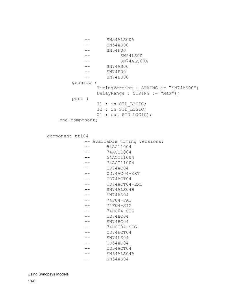
13-8
Using Synopsys Models
-- SN54ALS00A -- SN54AS00 -- SN54F00 -- SN54LS00 -- SN74ALS00A -- SN74AS00 -- SN74F00 -- SN74LS00
generic ( TimingVersion : STRING := “SN74AS00”;DelayRange : STRING := “Max”);
port (I1 : in STD_LOGIC;I2 : in STD_LOGIC;O1 : out STD_LOGIC);
end component;
component ttl04 -- Available timing versions:
-- 54AC11004 -- 74AC11004 -- 54ACT11004 -- 74ACT11004 -- CD74AC04 -- CD74AC04-EXT -- CD74ACT04 -- CD74ACT04-EXT -- SN74ALS04B -- SN74AS04 -- 74F04-FAI -- 74F04-SIG -- 74HC04-SIG -- CD74HC04 -- SN74HC04 -- 74HCT04-SIG -- CD74HCT04 -- SN74LS04 -- CD54AC04 -- CD54ACT04 -- SN54ALS04B -- SN54AS04
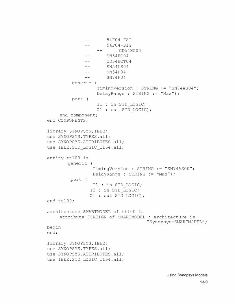
13-9
Using Synopsys Models
-- 54F04-FAI -- 54F04-SIG
-- CD54HC04 -- SN54HC04 -- CD54HCT04 -- SN54LS04 -- SN54F04 -- SN74F04
generic (TimingVersion : STRING := “SN74AS04”;DelayRange : STRING := “Max”);
port (I1 : in STD_LOGIC;O1 : out STD_LOGIC);
end component;end COMPONENTS;
library SYNOPSYS,IEEE;use SYNOPSYS.TYPES.all;use SYNOPSYS.ATTRIBUTES.all;use IEEE.STD_LOGIC_1164.all;
entity ttl00 is generic (
TimingVersion : STRING := “SN74AS00”; DelayRange : STRING := “Max”);
port ( I1 : in STD_LOGIC; I2 : in STD_LOGIC; O1 : out STD_LOGIC);
end ttl00;
architecture SMARTMODEL of ttl00 isattribute FOREIGN of SMARTMODEL : architecture is
“Synopsys:SMARTMODEL”;beginend;
library SYNOPSYS,IEEE;use SYNOPSYS.TYPES.all;use SYNOPSYS.ATTRIBUTES.all;use IEEE.STD_LOGIC_1164.all;
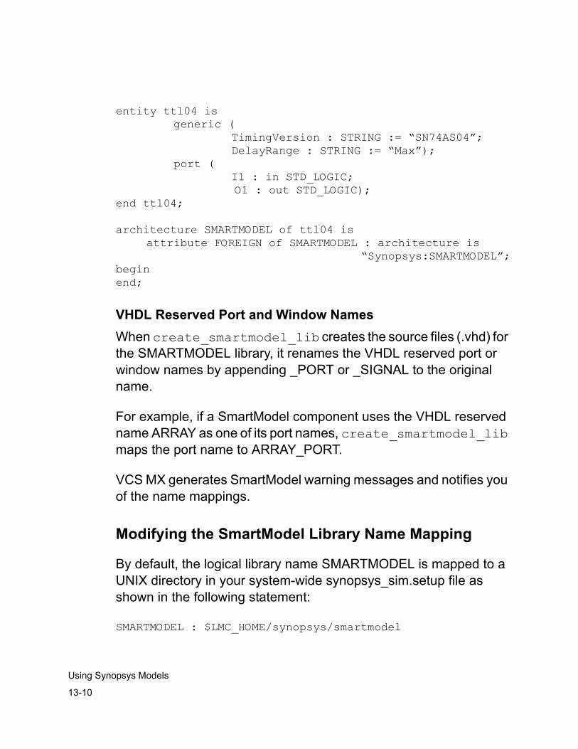
13-10
Using Synopsys Models
entity ttl04 is generic (
TimingVersion : STRING := “SN74AS04”; DelayRange : STRING := “Max”);
port ( I1 : in STD_LOGIC;
O1 : out STD_LOGIC);end ttl04;
architecture SMARTMODEL of ttl04 isattribute FOREIGN of SMARTMODEL : architecture is
“Synopsys:SMARTMODEL”;beginend;
VHDL Reserved Port and Window NamesWhen create_smartmodel_lib creates the source files (.vhd) for the SMARTMODEL library, it renames the VHDL reserved port or window names by appending _PORT or _SIGNAL to the original name.
For example, if a SmartModel component uses the VHDL reserved name ARRAY as one of its port names, create_smartmodel_lib maps the port name to ARRAY_PORT.
VCS MX generates SmartModel warning messages and notifies you of the name mappings.
Modifying the SmartModel Library Name Mapping
By default, the logical library name SMARTMODEL is mapped to a UNIX directory in your system-wide synopsys_sim.setup file as shown in the following statement:
SMARTMODEL : $LMC_HOME/synopsys/smartmodel
13-11
Using Synopsys Models
Synopsys recommends that you use the default SMARTMODEL library name mapping. The create_smartmodel_lib utility stores the analyzed source files in a directory as specified by the SMARTMODEL library name mapping.
If you change the default SMARTMODEL library name mapping, you must invoke the create_smartmodel_lib utility to reanalyze the source files. (See, the “Creating the SmartModel VHDL Library” section for more information about creating and analyzing SmartModel library source files.)
To change the default mapping, specify a different path in your local synopsys_sim.setup file. For example, you can add the following line to the synopsys_sim.setup file in your home directory:
SMARTMODEL : ~joe/smartmodel
To determine the current SMARTMODEL library mapping, type the following command at the prompt:
% show_setup -lib
Using SmartModels in VHDL Source Files
To use SmartModel components in the VHDL source file of your design, you must
• Specify the SMARTMODEL library in your VHDL design.
• Instantiate the SmartModel component.
After you use the SmartModel component in your source file, you can analyze and simulate your design.
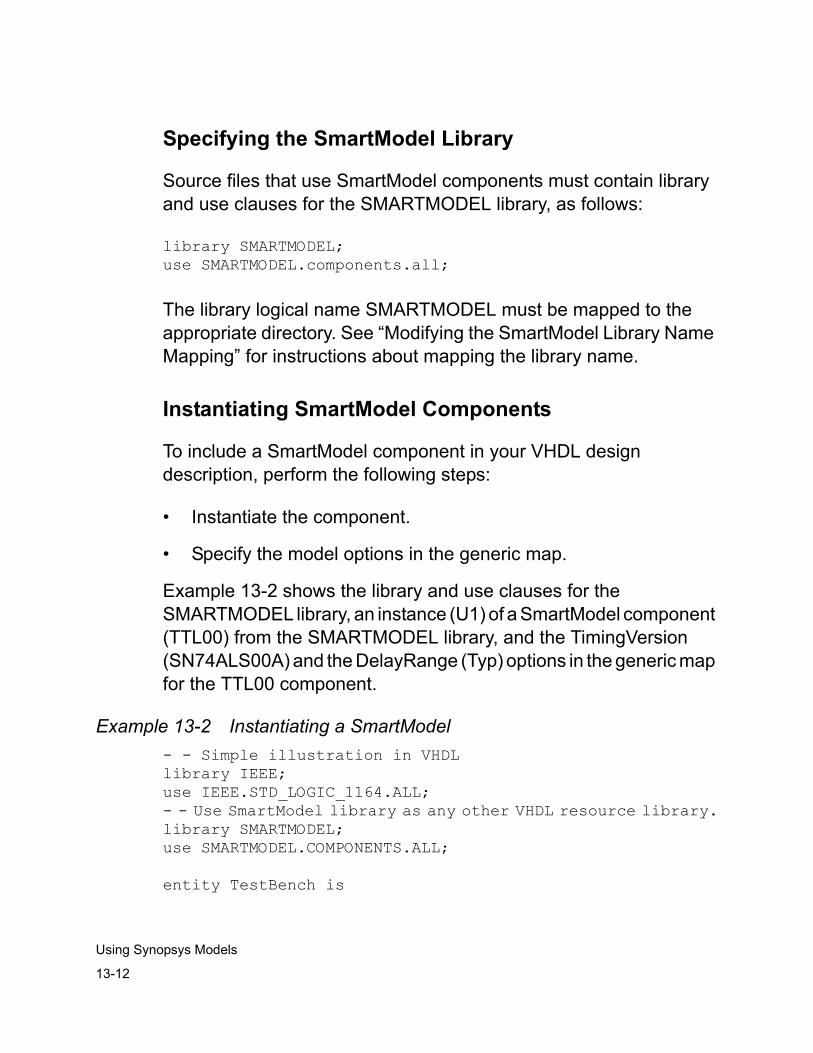
13-12
Using Synopsys Models
Specifying the SmartModel Library
Source files that use SmartModel components must contain library and use clauses for the SMARTMODEL library, as follows:
library SMARTMODEL;use SMARTMODEL.components.all;
The library logical name SMARTMODEL must be mapped to the appropriate directory. See “Modifying the SmartModel Library Name Mapping” for instructions about mapping the library name.
Instantiating SmartModel Components
To include a SmartModel component in your VHDL design description, perform the following steps:
• Instantiate the component.
• Specify the model options in the generic map.
Example 13-2 shows the library and use clauses for the SMARTMODEL library, an instance (U1) of a SmartModel component (TTL00) from the SMARTMODEL library, and the TimingVersion (SN74ALS00A) and the DelayRange (Typ) options in the generic map for the TTL00 component.
Example 13-2 Instantiating a SmartModel- - Simple illustration in VHDL library IEEE;use IEEE.STD_LOGIC_1164.ALL;- - Use SmartModel library as any other VHDL resource library.library SMARTMODEL;use SMARTMODEL.COMPONENTS.ALL;
entity TestBench is
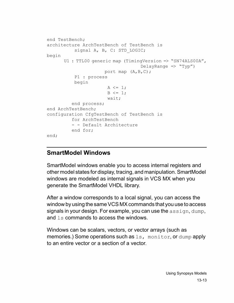
13-13
Using Synopsys Models
end TestBench;architecture ArchTestBench of TestBench is signal A, B, C: STD_LOGIC;begin U1 : TTL00 generic map (TimingVersion => “SN74ALS00A”, DelayRange => “Typ”) port map (A,B,C); P1 : process begin A <= 1; B <= 1; wait; end process;end ArchTestBench;configuration CfgTestBench of TestBench is for ArchTestBench - - Default Architecture end for;end;
SmartModel Windows
SmartModel windows enable you to access internal registers and other model states for display, tracing, and manipulation. SmartModel windows are modeled as internal signals in VCS MX when you generate the SmartModel VHDL library.
After a window corresponds to a local signal, you can access the window by using the same VCS MX commands that you use to access signals in your design. For example, you can use the assign, dump, and ls commands to access the windows.
Windows can be scalars, vectors, or vector arrays (such as memories.) Some operations such as ls, monitor, or dump apply to an entire vector or a section of a vector.
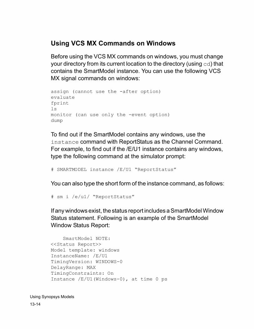
13-14
Using Synopsys Models
Using VCS MX Commands on Windows
Before using the VCS MX commands on windows, you must change your directory from its current location to the directory (using cd) that contains the SmartModel instance. You can use the following VCS MX signal commands on windows:
assign (cannot use the -after option)evaluatefprintlsmonitor (can use only the -event option)dump
To find out if the SmartModel contains any windows, use the instance command with ReportStatus as the Channel Command. For example, to find out if the /E/U1 instance contains any windows, type the following command at the simulator prompt:
# SMARTMODEL instance /E/U1 “ReportStatus”
You can also type the short form of the instance command, as follows:
# sm i /e/u1/ “ReportStatus”
If any windows exist, the status report includes a SmartModel Window Status statement. Following is an example of the SmartModel Window Status Report:
SmartModel NOTE:<<Status Report>>Model template: windowsInstanceName: /E/U1TimingVersion: WINDOWS-0DelayRange: MAXTimingConstraints: OnInstance /E/U1(Windows-0), at time 0 ps
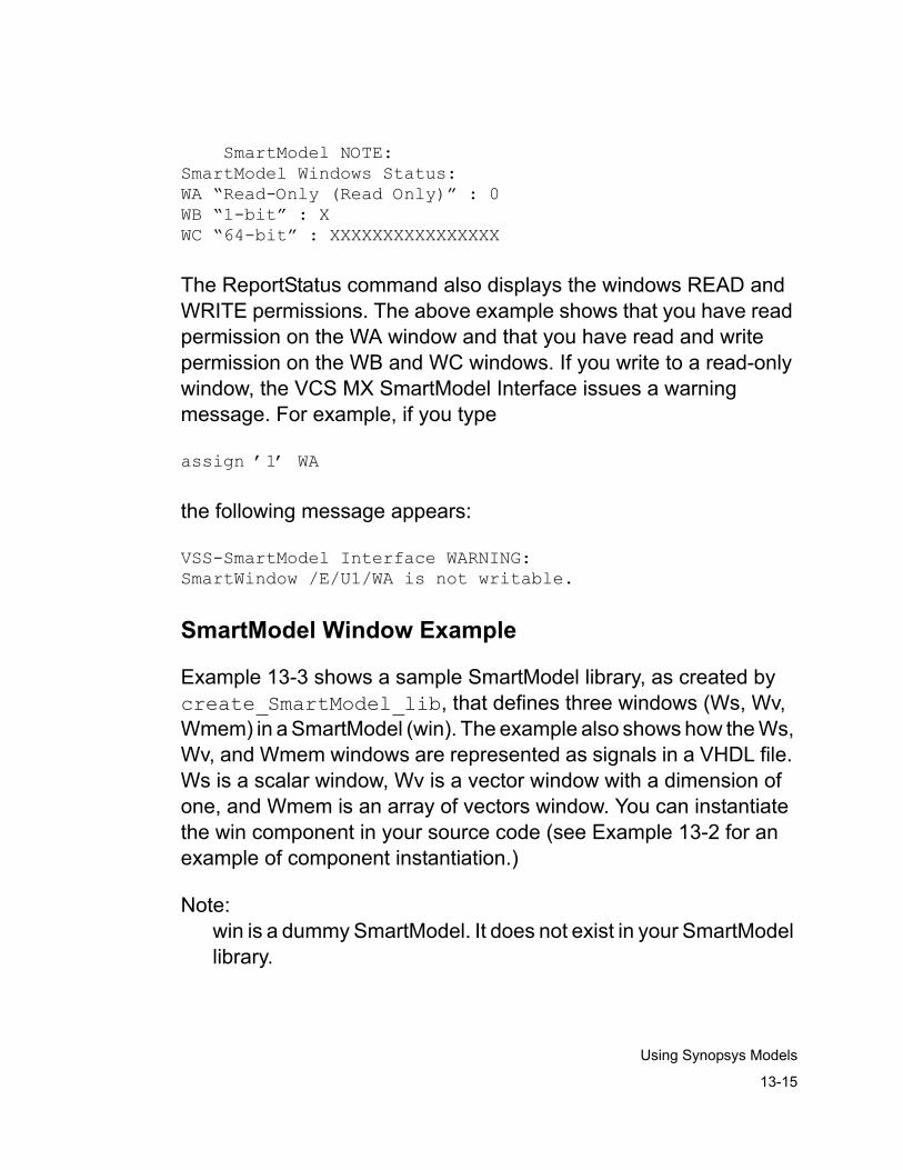
13-15
Using Synopsys Models
SmartModel NOTE:SmartModel Windows Status:WA “Read-Only (Read Only)” : 0WB “1-bit” : XWC “64-bit” : XXXXXXXXXXXXXXXX
The ReportStatus command also displays the windows READ and WRITE permissions. The above example shows that you have read permission on the WA window and that you have read and write permission on the WB and WC windows. If you write to a read-only window, the VCS MX SmartModel Interface issues a warning message. For example, if you type
assign ’1’ WA
the following message appears:
VSS-SmartModel Interface WARNING:SmartWindow /E/U1/WA is not writable.
SmartModel Window Example
Example 13-3 shows a sample SmartModel library, as created by create_SmartModel_lib, that defines three windows (Ws, Wv, Wmem) in a SmartModel (win). The example also shows how the Ws, Wv, and Wmem windows are represented as signals in a VHDL file. Ws is a scalar window, Wv is a vector window with a dimension of one, and Wmem is an array of vectors window. You can instantiate the win component in your source code (see Example 13-2 for an example of component instantiation.)
Note:win is a dummy SmartModel. It does not exist in your SmartModel library.
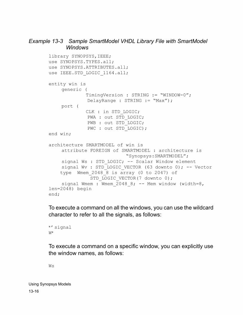
13-16
Using Synopsys Models
Example 13-3 Sample SmartModel VHDL Library File with SmartModel Windows
library SYNOPSYS,IEEE;use SYNOPSYS.TYPES.all;use SYNOPSYS.ATTRIBUTES.all;use IEEE.STD_LOGIC_1164.all;
entity win isgeneric (
TimingVersion : STRING := “WINDOW-0”;DelayRange : STRING := “Max”);
port ( CLK : in STD_LOGIC;
PWA : out STD_LOGIC;PWB : out STD_LOGIC;PWC : out STD_LOGIC);
end win;
architecture SMARTMODEL of win isattribute FOREIGN of SMARTMODEL : architecture is
“Synopsys:SMARTMODEL”;signal Ws : STD_LOGIC; -- Scalar Window elementsignal Wv : STD_LOGIC_VECTOR (63 downto 0); -- Vector
type Wmem_2048_8 is array (0 to 2047) of STD_LOGIC_VECTOR(7 downto 0);
signal Wmem : Wmem_2048_8; -- Mem window (width=8, len=2048) beginend;
To execute a command on all the windows, you can use the wildcard character to refer to all the signals, as follows:
*’signalW*
To execute a command on a specific window, you can explicitly use the window names, as follows:
Ws
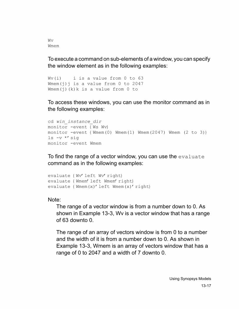
13-17
Using Synopsys Models
WvWmem
To execute a command on sub-elements of a window, you can specify the window element as in the following examples:
Wv(i) i is a value from 0 to 63Wmem(j)j is a value from 0 to 2047Wmem(j)(k)k is a value from 0 to
To access these windows, you can use the monitor command as in the following examples:
cd win_instance_dirmonitor -event {Ws Wv} monitor -event {Wmem(0) Wmem(1) Wmem(2047) Wmem (2 to 3)}ls -v *’sigmonitor -event Wmem
To find the range of a vector window, you can use the evaluate command as in the following examples:
evaluate {Wv’left Wv’right}evaluate {Wmem’left Wmem’right}evaluate {Wmem(x)’left Wmem(x)’right}
Note:The range of a vector window is from a number down to 0. As shown in Example 13-3, Wv is a vector window that has a range of 63 downto 0.
The range of an array of vectors window is from 0 to a number and the width of it is from a number down to 0. As shown in Example 13-3, Wmem is an array of vectors window that has a range of 0 to 2047 and a width of 7 downto 0.
13-18
Using Synopsys Models
SmartModel Window Precautions
Synopsys recommends that you do not use the monitor or dump commands on window sections that contain a large number of vectors. In general, the larger the number of vectors that you monitor, the slower the performance of the Simulator. Use the monitor or dump command on window sections containing a small numbers of vectors.
If you monitor or trace window sections greater than 64 vectors, the VCS MX SmartModel Interface issues a warning message informing you that the performance of the simulator is drastically affected.
The SmartModel Interface does not support windows created from SCF files. For more information about SCF files, refer to the SmartModel documentation.
Error Messages
SmartModel messages issued by VCS MX start with the following line:
VSS-SmartModel Interface
SmartModel messages issued by Synopsys SmartModels start with the following line:
SmartModel
There are four types of SmartModel messages from Synopsys SmartModels: Warning, Trace, Note, and Error.
Warning, Trace, and Note messages have the following format:
SmartModel Warning:
13-19
Using Synopsys Models
scsim,432:
SmartModel Trace:Trace is turned on. SmartModel Instance U1 (SCF-0), at time 200NS.
SmartModel Note:Reading configuration file: ’scf.1’.Instance E/UT (SCF-0), at time 0NS.
An Error message has the following format:
**Error: scsim,431:SmartModel FATAL ERROR:The LMC_HOME environment variable has not been set.
For information about specific messages, see SmartModel documentation.
Modifying the Timing Files
Normally, you use the default timing file for a SmartModel in your simulation. However, you can edit the values in the default file to use in your simulation.
For more information about editing the timing file and using it in your simulation, see the SmartModel documentation.
LM-Family Hardware Modeler Interface
The interface for using LM-family hardware modelers with VCS MX involves these primary concepts:
13-20
Using Synopsys Models
• Before You Start
• Setting Up the Environment
• Creating VHDL Model Support Files
• Modifying LM-family Shell Software Files
• Analyzing and Linking the Design
• Simulating the Design
• Error messages
• LM-family modeler example
Before You Start
The LM-family hardware modeler uses actual hardware devices to model their behavior during simulation. The modeler applies the inputs to the physical device, evaluates the device behavior, and returns the results to VCS MX through the interface.
Figure 13-1 shows the relationship of the LM-family modelers to VCS MX. When you invoke the Simulator (scsim), it accesses the LM-family Shell Software files and manages the Ethernet link communications with the modeler.
Interface Benefits
Following are the primary benefits of the Synopsys’ LM-family hardware modeler interface:
• Provides model-independence
13-21
Using Synopsys Models
The interface allows you to simulate different configurations without generating a different simulator for each hardware model.
With model-independence, you can also create your own hardware models to use with the Simulator. For example, you can simulate a proprietary microprocessor that is still in development.
• Uses standard VHDL code for hardware model support
Because the hardware modeler uses standard VHDL code for the interface, it is a straightforward task for you to modify a VHDL design to use LM-family hardware models.
Documentation for Operating the Modeler
Except for the Synopsys restrictions on Shell Software files, use Hardware Models documentation to install and operate the modeler.
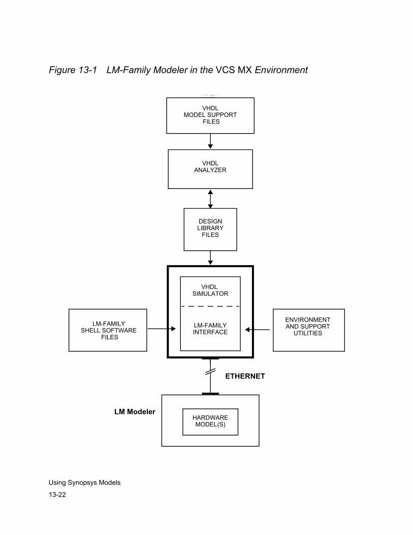
13-22
Using Synopsys Models
Figure 13-1 LM-Family Modeler in the VCS MX Environment
VHDL SIMULATOR
LM-FAMILYINTERFACE
VHDLANALYZER
DESIGNLIBRARY
FILES
DESIGNLIBRARY
FILES
DESIGNLIBRARY
FILES
VHDLSOURCE
FILES
VHDLSOURCE
FILES
VHDLMODEL SUPPORT
FILES
VHDLSOURCE
FILES
VHDLSOURCE
FILESVHDL
MODEL SUPPORT FILES
HARDWAREMODEL(S)
ETHERNET
LM Modeler
ENVIRONMENTAND SUPPORT
UTILITIES
VHDLSOURCE
FILES
VHDLSOURCE
FILES
LM-FAMILYSHELL SOFTWARE
FILES
13-23
Using Synopsys Models
Logic Types Requirement
VCS MX requires you to use std_logic defined types for LM-family models, unless you provide a map between std_logic and a user-defined enumeration type.
LM-Family Utilities
Synopsys provides two utilities, lm and lmdaemon, for you to use with the LM-family modeler.
lm UtilityThe lm utility is a menu-based program for creating and verifying models and for performing maintenance and diagnostic functions on the modeler. See the Hardware Models documentation for complete information.
lmdaemon UtilityThe lmdaemon utility runs as a system background process (daemon) and monitors activity on the LM-family hardware modeler. The lmdaemon utility has two functions:
• It deletes any instance information that has been idle in the hardware modeler for more than a user-specified time limit.
• It automatically reboots the modeler if the modeler crashes.
The use of lmdaemon is optional.
13-24
Using Synopsys Models
Setting up the Environment
The LM-family modeler must be installed before you set up the environment. For information on installing the LM-family modeler, see the Logic Modeling documentation.
Set up your environment by performing the following steps:
1. Set the LM_DIR and LM_LIB environment variables. You can set these variables manually from the UNIX prompt, or you can add the settings to your .cshrc file so that they are automatically set when you invoke a new shell.
unix% setenv LM_DIR pathname/lm_dirunix% setenv LM_LIB pathname/models:pathname/maps
Replace pathname with the LM software installation pathname.
2. Use the lm utility to verify that the hardware modeler is properly installed in the Ethernet network environment where you are using VCS MX. See the LM-family documentation for more information on the lm utility.
3. Ensure that you have the appropriate license in your license file for the LM-family hardware modeler.
13-25
Using Synopsys Models
Creating VHDL Model Support Files
For each LM-family model, you must provide
• A file containing an entity-architecture pair declaration, so that the VHDL design can reference it later in a component instantiation statement.
• A package for defining constants, declaring components, and instantiating components.
• A test bench or input stimulus file for exercising the model.
These can be in one file or in separate files. The input stimulus file also normally contains an instantiation of the model and can contain any processes necessary to simulate the support circuitry for the model (for example, clocks signals.)
Using the create_hwmodel_shell UtilityYou can use the utility create_hwmodel_shell to generate the entity-architecture pair declaration. This utility is a simple awk script that reads the model’s NAM file and produces the model’s VHDL shell.
The syntax of create_hwmodel_shell is
create_hwmodel_shell model.NAM outfile.vhd
Entity Declaration
Example 13-4 shows the basic format of an entity declaration for the LM-family modeler. Example 13-5 shows the actual entity declaration for the MC68020 model. Note that only some of the generic types are used in Example 13-5; the others will have their default values.
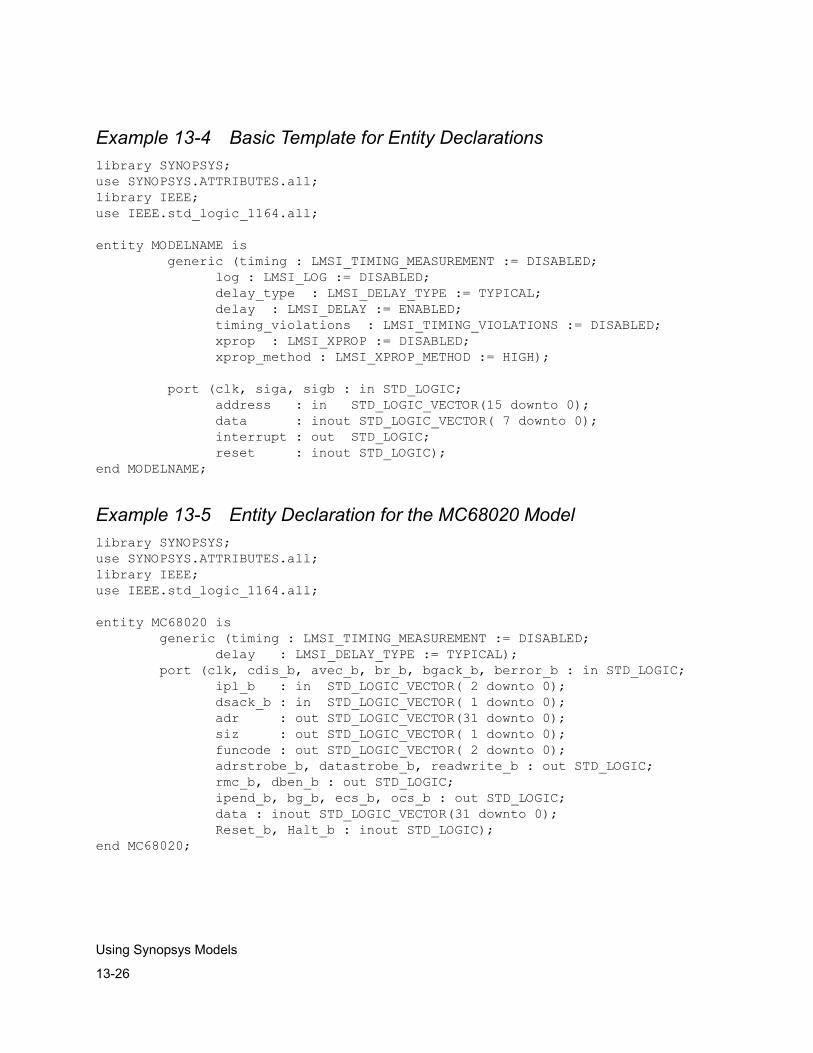
13-26
Using Synopsys Models
Example 13-4 Basic Template for Entity Declarationslibrary SYNOPSYS;use SYNOPSYS.ATTRIBUTES.all;library IEEE;use IEEE.std_logic_1164.all;
entity MODELNAME is generic (timing : LMSI_TIMING_MEASUREMENT := DISABLED; log : LMSI_LOG := DISABLED; delay_type : LMSI_DELAY_TYPE := TYPICAL; delay : LMSI_DELAY := ENABLED; timing_violations : LMSI_TIMING_VIOLATIONS := DISABLED; xprop : LMSI_XPROP := DISABLED; xprop_method : LMSI_XPROP_METHOD := HIGH);
port (clk, siga, sigb : in STD_LOGIC; address : in STD_LOGIC_VECTOR(15 downto 0); data : inout STD_LOGIC_VECTOR( 7 downto 0); interrupt : out STD_LOGIC; reset : inout STD_LOGIC);end MODELNAME;
Example 13-5 Entity Declaration for the MC68020 Modellibrary SYNOPSYS;use SYNOPSYS.ATTRIBUTES.all;library IEEE;use IEEE.std_logic_1164.all;
entity MC68020 is generic (timing : LMSI_TIMING_MEASUREMENT := DISABLED; delay : LMSI_DELAY_TYPE := TYPICAL); port (clk, cdis_b, avec_b, br_b, bgack_b, berror_b : in STD_LOGIC; ipl_b : in STD_LOGIC_VECTOR( 2 downto 0); dsack_b : in STD_LOGIC_VECTOR( 1 downto 0); adr : out STD_LOGIC_VECTOR(31 downto 0); siz : out STD_LOGIC_VECTOR( 1 downto 0); funcode : out STD_LOGIC_VECTOR( 2 downto 0); adrstrobe_b, datastrobe_b, readwrite_b : out STD_LOGIC; rmc_b, dben_b : out STD_LOGIC; ipend_b, bg_b, ecs_b, ocs_b : out STD_LOGIC; data : inout STD_LOGIC_VECTOR(31 downto 0); Reset_b, Halt_b : inout STD_LOGIC);end MC68020;
13-27
Using Synopsys Models
The VHDL library and use clauses at the top of the file allow you to access the types and attributes you plan to use in your VHDL code, so the Simulator can communicate with the modeler.
Entity Name RestrictionsThe entity name must meet the file naming restrictions of the OS that is running on your platform. VCS MX requires that the entity name match the device name.
Using GenericsYou can use the generic clause in an entity declaration to
• Specify the source of the timing values passed from the Modeler to the Simulator.
• Specify the delay type (minimum, typical, or maximum) the Simulator will use at evaluation time.
• Enable or disable the propagation of unknown (’X’) values during simulation.
• Determine the method used to propagate unknown (’X’) values.
• Enable or disable delay calculations, violation-reporting, and test-vector logging.
Use the LM-family Shell Software files to control other settings, such as the hostname of the target modeler.
The following sections describe the generics you can use with the LM-family hardware modeler. If you do not specify a value for a generic, the Simulator uses the default value. The Simulator reports an error if you attempt to assign values other than the ones explained below and defined in the SYNOPSYS.ATTRIBUTES package.
13-28
Using Synopsys Models
Specifying Timing SourceYou can choose two sources of timing values for your simulation session:
• Actual pin-to-pin timing measurements
• Timing measurements from a timing (.TMG) file
The following possible values of LMSI_TIMING_MEASUREMENT in the generic clause select the timing source:
ENABLEDModeler measures and records the actual pin-to-pin timing values and passes them to the Simulator.
DISABLEDModeler passes to the Simulator the pin-to-pin timing values from the .TMG file. DISABLED is the default value of LMSI_TIMING_MEASUREMENT.
Example 13-5 contains the following line:
generic (timing LMSI_TIMING_MEASUREMENT := DISABLED);
The actual identifier name (for example, timing) is not important. If two or more identifiers have type LMSI_TIMING_MEASUREMENT, the modeler issues a warning and uses the default value.
The MC68020 microprocessor example uses the pin-to-pin delay values defined in the MC68020.TMG file rather than the actual measured values.

13-29
Using Synopsys Models
Specifying Delay TypeAt evaluation time, the modeler returns each pin value with three delay values: minimum, typical, and maximum. The delay values can come from a record of actual device timing measurements or from a .TMG file, as explained in the previous section. By adding an identifier of type LMSI_DELAY_TYPE to the generic clause of your entity declaration, you can indicate which delay value the Simulator uses.
Table 13-1 lists the permitted values for the delay generic as defined in the SYNOPSYS.ATTRIBUTES package.
Table 13-1 Delay Generic Types
For example, Example 13-5 has the following lines:
generic (timing : LMSI_TIMING_MEASUREMENT := DISABLED; delay_type : LMSI_DELAY_TYPE := TYPICAL);
You select the actual identifier name (for example, delay_type). If two or more identifiers have type LMSI_DELAY_TYPE, the modeler issues a warning and uses the default value. Example 13-4 and Example 13-5 use the TYPICAL delay (which is the default).
Turning ’X’ Propagation On and OffYou can use generics to control the propagation of Unknown (’X’) values from input pins to output pins of LM-family hardware models.
Type Allowable Values
LMSI_DELAY_TYPE MINIMUM
TYPICAL (default)
MAXIMUM
13-30
Using Synopsys Models
A generic of type LMSI_XPROP in an entity declaration enables or disables ’X’ propagation for all instances of that entity. (To turn ’X’ propagation on and off for specific pins, use the simulator command lmsi xpropagation, described below.) By default, ’X’ propagation is turned off.
Note:An on_unknown statement in a Shell Software file overrides both command-line and generic ’X’ propagation settings.
The entity declaration in Example 13-4 contains the following line:
generic (xprop : LMSI_XPROP := DISABLED);
With this setting, all instances of MODELNAME will have ’X’ propagation turned off.
The possible values for a generic of type LMSI_XPROP are ENABLED and DISABLED.
The actual identifier you use to name the generic (in the example, xprop) is not important. If two or more identifiers have type LMSI_XPROP, the modeler issues a warning and uses the default value.
Specifying the Propagation MethodWhen you enable ’X’ propagation, you can specify any of the four methods used by LM-family modelers to propagate unknown values: PREVIOUS, HIGH, LOW, and FLOAT. The default method is PREVIOUS. See your modeler documentation for a description of the propagation methods.
13-31
Using Synopsys Models
A generic of type LMSI_XPROP_METHOD in an entity declaration determines the method of ’X’ propagation for all instances of that entity.
The entity declaration in Example 13-4 contains the following line:
generic (xprop_method : LMSI_XPROP_METHOD := HIGH);
With this setting, the modeler will use the HIGH method when propagating unknown values for all instances of MODELNAME.
The possible values for a generic of type LMSI_XPROP_METHOD are PREVIOUS, HIGH, LOW, and FLOAT.
The actual identifier you use to name the generic (in the example, xprop_method) is not important. If two or more identifiers have type LMSI_XPROP_METHOD, the modeler issues a warning and uses the default value.
Turning Delay Calculation On and OffYou can use generics to control whether the LM-family modeler performs delay calculations. Disabling the calculations increases simulation speed.
By default, delay calculation is enabled. When you turn delay calculation off for a given device, the simulator assumes a unit delay of one simulation time tick.
A generic of type LMSI_DELAY in an entity declaration determines whether or not delay calculations are performed for all instances of that entity. The entity declaration in Example 13-4 contains the following line:
generic (delay : LMSI_DELAY := ENABLED);
13-32
Using Synopsys Models
With this setting, all instances of MODELNAME will have delay calculation turned on.
The possible values for a generic of type LMSI_DELAY are ENABLED and DISABLED.
The actual identifier you use to name the generic (in the example, delay) is not important. If two or more identifiers have type LMSI_DELAY, the modeler issues a warning and uses the default value.
Turning Timing-Violation Reports On and OffYou can use generics to control whether the LM-family modeler reports timing violations. Disabling the reports increases simulation speed.
Note:A report timing_violation statement in a Shell Software file overrides both command-line and generic violation-reporting settings.
By default, violation-reporting is enabled. A generic of type LMSI_TIMING_VIOLATIONS in an entity declaration determines whether or not timing violations are reported for all instances of that entity. The entity declaration in Example 13-4 contains the following line:
generic (timing_violations : LMSI_TIMING_VIOLATIONS := DISABLED);
With this setting, all instances of MODELNAME will have violation reporting turned off.
13-33
Using Synopsys Models
The possible values for a generic of type LMSI_TIMING_VIOLATIONS are ENABLED and DISABLED.
The actual identifier you use to name the generic (in the example, timing_violations) is not important. If two or more identifiers have type LMSI_TIMING_VIOLATIONS, the modeler issues a warning and uses the default value.
Logging Test VectorsYou can use generics to control whether the LM-family modeler logs test vectors. By default, test-vector logging is off.
The entity declaration in Example 1-1 contains the following line:
generic (log : LMSI_LOG := DISABLED);
With this setting, all instances of MODELNAME will have test-vector logging turned off.
The possible values for a generic of type LMSI_LOG are ENABLED and DISABLED.
The actual identifier you use to name the generic (in the example, log) is not important. If two or more identifiers have type LMSI_LOG, the modeler issues a warning and uses the default value.
Architecture Declaration
The attribute FOREIGN in an architecture declaration indicates to the Analyzer (vhdlan) that the architecture is not fully described in VHDL. The value of FOREIGN indicates which interface (LM-family modeler, SmartModel, or VHPI) contains the complete architecture.

13-34
Using Synopsys Models
Example 13-6 shows the basic format of the architecture declaration for an architecture in the LM-family modeler. The architecture declaration is empty except for the attribute specification, which instructs the Simulator to use the LM-family modeler.
Example 13-6 Basic Template for Architecture Declarationsarchitecture architecture of entity_name is attribute FOREIGN of architecture: architecture is ”Synopsys:LMSI”;beginend;
You must use the attribute value "Synopsys:LMSI" for the LM-family modeler; the value is case-insensitive.
Example 13-7 shows the architecture declaration for an MC68020 model. It demonstrates the case insensitivity of the FOREIGN attribute value ”synopsys:lmsi”.
Example 13-7 Architecture Declaration for the MC68020 Modellibrary SYNOPSYS;use SYNOPSYS.ATTRIBUTES.all;
architecture LMSI of MC68020 is attribute FOREIGN of LMSI: architecture is ”synopsys:lmsi”;beginend;
Model Package
You can provide a package for defining constant values and declaring components. Example 13-8 shows a package for the MC68020 model example.
Example 13-8 Package Used with the MC68020 Modellibrary SYNOPSYS;use SYNOPSYS.ATTRIBUTES.all;library IEEE;
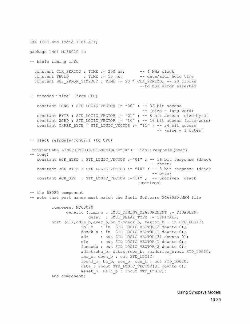
13-35
Using Synopsys Models
use IEEE.std_logic_1164.all;
package LMSI_MC68020 is
-- basic timing info
constant CLK_PERIOD : TIME := 250 ns; -- 4 MHz clock constant THOLD : TIME := 50 ns; -- data/addr hold time constant BUS_ERROR_TIMEOUT : TIME := 20 * CLK_PERIOD; -- 20 clocks --to bus error asserted
-- encoded ’size’ (from CPU)
constant LONG : STD_LOGIC_VECTOR := ”00” ; -- 32 bit access -- (size = long word) constant BYTE : STD_LOGIC_VECTOR := ”01” ; -- 8 bit access (size=byte) constant WORD : STD_LOGIC_VECTOR := ”10” ; -- 16 bit access (size=word) constant THREE_BYTE : STD_LOGIC_VECTOR := ”11” ; -- 24 bit access -- (size = 3 bytes)
-- dsack response/control (to CPU)
constant ACK_LONG : STD_LOGIC_VECTOR :=”00” ; -- 32 bit response (dsack -- long) constant ACK_WORD : STD_LOGIC_VECTOR :=”01” ; -- 16 bit response (dsack -- short) constant ACK_BYTE : STD_LOGIC_VECTOR := ”10” ; -- 8 bit response (dsack -- byte) constant ACK_OFF : STD_LOGIC_VECTOR :=”11” ; -- undriven (dsack
undriven)
-- the 68020 component-- note that port names must match the Shell Software MC68020.NAM file
component MC68020 generic (timing : LMSI_TIMING_MEASUREMENT := DISABLED; delay : LMSI_DELAY_TYPE := TYPICAL); port (clk,cdis_b,avec_b,br_b,bgack_b, berror_b : in STD_LOGIC; ipl_b : in STD_LOGIC_VECTOR(2 downto 0); dsack_b : in STD_LOGIC_VECTOR(1 downto 0); adr : out STD_LOGIC_VECTOR(31 downto 0); siz : out STD_LOGIC_VECTOR(1 downto 0); funcode : out STD_LOGIC_VECTOR(2 downto 0); adrstrobe_b, datastrobe_b, readwrite_b:out STD_LOGIC; rmc_b, dben_b : out STD_LOGIC; ipend_b, bg_b, ecs_b, ocs_b : out STD_LOGIC; data : inout STD_LOGIC_VECTOR(31 downto 0); Reset_b, Halt_b : inout STD_LOGIC); end component;

13-36
Using Synopsys Models
end LMSI_MC68020;
Input Stimulus and Component Instantiation
You must provide input stimulus to initialize the model. Normally you also include an instantiation of the component.
Example 13-9 shows declarations for input signals and their initial values, their output signals, and the instantiation of a component, U0, that uses these signals.
Example 13-9 Component Instantiation Used with the MC68020 Modellibrary SYNOPSYS;use SYNOPSYS.ATTRIBUTES.all;use SYNOPSYS.BV_ARITHMETIC.all;library IEEE;use IEEE.std_logic_1164.all; use IEEE.std_logic_arith.all;use WORK.LMSI_MC68020.all;
entity E isend E;
architecture A of E is
-- inputs signal clk : STD_LOGIC := ’0’ ; -- start off clock low signal reset : STD_LOGIC := ’L’ ; -- start off in reset mode signal halt : STD_LOGIC := ’H’ ; -- ... with reset on, no halt signal dsack : STD_LOGIC_VECTOR(1 downto 0) := ACK_OFF; -- data strobe --ack (start ’OFF’) signal data : STD_LOGIC_VECTOR(31 downto 0) := (others => ’Z’); -- data -- bus
-- outputs signal as : STD_LOGIC; -- address strobe signal ds : STD_LOGIC; -- data strobe signal rw : STD_LOGIC; -- read/write state (read = 1) signal addr : STD_LOGIC_VECTOR(31 downto 0); -- address bus signal size : STD_LOGIC_VECTOR(1 downto 0); -- cycle size
-- unused inputs
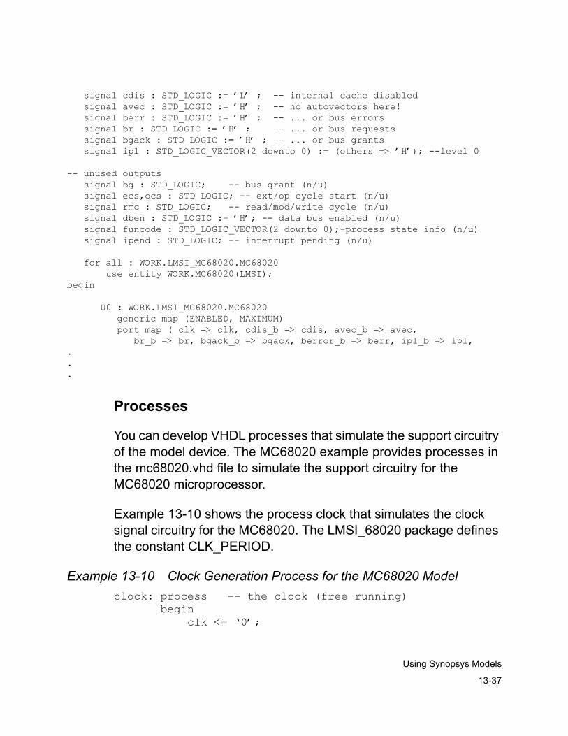
13-37
Using Synopsys Models
signal cdis : STD_LOGIC := ’L’ ; -- internal cache disabled signal avec : STD_LOGIC := ’H’ ; -- no autovectors here! signal berr : STD_LOGIC := ’H’ ; -- ... or bus errors signal br : STD_LOGIC := ’H’ ; -- ... or bus requests signal bgack : STD_LOGIC := ’H’ ; -- ... or bus grants signal ipl : STD_LOGIC_VECTOR(2 downto 0) := (others => ’H’); --level 0
-- unused outputs signal bg : STD_LOGIC; -- bus grant (n/u) signal ecs,ocs : STD_LOGIC; -- ext/op cycle start (n/u) signal rmc : STD_LOGIC; -- read/mod/write cycle (n/u) signal dben : STD_LOGIC := ’H’; -- data bus enabled (n/u) signal funcode : STD_LOGIC_VECTOR(2 downto 0);-process state info (n/u) signal ipend : STD_LOGIC; -- interrupt pending (n/u)
for all : WORK.LMSI_MC68020.MC68020 use entity WORK.MC68020(LMSI);begin
U0 : WORK.LMSI_MC68020.MC68020 generic map (ENABLED, MAXIMUM) port map ( clk => clk, cdis_b => cdis, avec_b => avec, br_b => br, bgack_b => bgack, berror_b => berr, ipl_b => ipl,...
Processes
You can develop VHDL processes that simulate the support circuitry of the model device. The MC68020 example provides processes in the mc68020.vhd file to simulate the support circuitry for the MC68020 microprocessor.
Example 13-10 shows the process clock that simulates the clock signal circuitry for the MC68020. The LMSI_68020 package defines the constant CLK_PERIOD.
Example 13-10 Clock Generation Process for the MC68020 Modelclock: process -- the clock (free running) begin clk <= ‘0’;
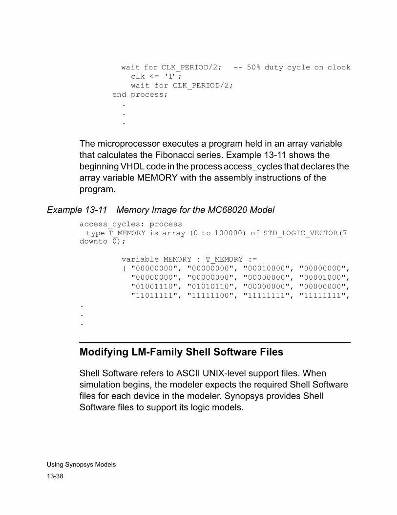
13-38
Using Synopsys Models
wait for CLK_PERIOD/2; -- 50% duty cycle on clock clk <= ‘1’; wait for CLK_PERIOD/2; end process;
.
.
.
The microprocessor executes a program held in an array variable that calculates the Fibonacci series. Example 13-11 shows the beginning VHDL code in the process access_cycles that declares the array variable MEMORY with the assembly instructions of the program.
Example 13-11 Memory Image for the MC68020 Modelaccess_cycles: process type T_MEMORY is array (0 to 100000) of STD_LOGIC_VECTOR(7 downto 0);
variable MEMORY : T_MEMORY := ( "00000000", "00000000", "00010000", "00000000", "00000000", "00000000", "00000000", "00001000", "01001110", "01010110", "00000000", "00000000", "11011111", "11111100", "11111111", "11111111",...
Modifying LM-Family Shell Software Files
Shell Software refers to ASCII UNIX-level support files. When simulation begins, the modeler expects the required Shell Software files for each device in the modeler. Synopsys provides Shell Software files to support its logic models.
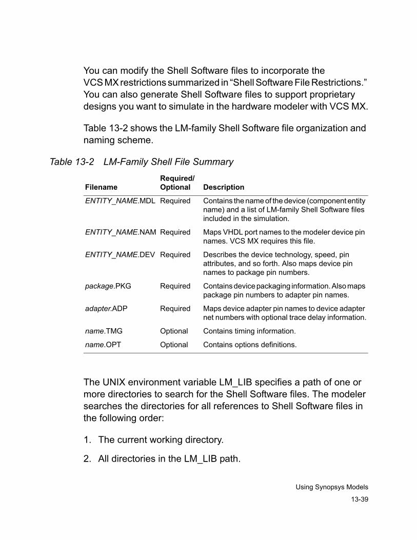
13-39
Using Synopsys Models
You can modify the Shell Software files to incorporate the VCS MX restrictions summarized in “Shell Software File Restrictions.” You can also generate Shell Software files to support proprietary designs you want to simulate in the hardware modeler with VCS MX.
Table 13-2 shows the LM-family Shell Software file organization and naming scheme.
Table 13-2 LM-Family Shell File Summary
The UNIX environment variable LM_LIB specifies a path of one or more directories to search for the Shell Software files. The modeler searches the directories for all references to Shell Software files in the following order:
1. The current working directory.
2. All directories in the LM_LIB path.
FilenameRequired/Optional Description
ENTITY_NAME.MDL Required Contains the name of the device (component entity name) and a list of LM-family Shell Software files included in the simulation.
ENTITY_NAME.NAM Required Maps VHDL port names to the modeler device pin names. VCS MX requires this file.
ENTITY_NAME.DEV Required Describes the device technology, speed, pin attributes, and so forth. Also maps device pin names to package pin numbers.
package.PKG Required Contains device packaging information. Also maps package pin numbers to adapter pin names.
adapter.ADP Required Maps device adapter pin names to device adapter net numbers with optional trace delay information.
name.TMG Optional Contains timing information.
name.OPT Optional Contains options definitions.
13-40
Using Synopsys Models
3. All immediate subdirectories of the directories in the LM_LIB path.
The environment variable LM_LIB is set when you source the $VCS_HOME/admin/setup/environ.* file during installation. You can modify LM_LIB to suite your environment. See the Hardware Models documentation for an explanation of the host-specific syntax for defining LM_LIB.
The following sections outline only the conventions and restrictions for the Shell Software files. See Hardware Models documentation for more information.
Shell Software File Restrictions
Synopsys imposes the following restrictions on the use of the LM-family Shell Software files:
• The .NAM file is required when using the LM-family interface.
At the last level of mapping device pins to names, you must map each pin name to a legal VHDL identifier.
The modeler can contain multiple mappings of names to a device pin. The .NAM file contains the topmost (last) level of mapping that you can use, and the .DEV file is one step of mapping below the .NAM file. At the last level mapping from either the .NAM or .DEV file, you must map each pin name to a legal VHDL identifier.
• At the last level of mapping, you must map the Shell Software-defined pin names to names of all uppercase letters.

13-41
Using Synopsys Models
All objects in the Shell Software files are case-sensitive, while in VHDL they are case-insensitive. Because VCS MX internally maps all object names to uppercase letters, Synopsys requires that all top level names be valid VHDL identifiers of all uppercase letters.
• The device name in the model (.MDL) file, the base name of the .MDL file, and the component entity name must be identical and in uppercase letters.
VCS MX gets the entity name from the base name of the .MDL file, not from the device_name parameter contained in the .MDL file.
The .MDL FileThe LM-family modeler requires an .MDL file for each device it models. Synopsys requires that the base name of this file, the component entity name, and the device name (device_name) contained in this file are identical. Additionally, use uppercase for all alphabetic characters in the filename.
The .MDL file serves as the header file for the Shell Software description of the device. It holds the name of the device and the names of all Shell Software files necessary for the simulation. The Simulator accesses all device-specific information such as names, timing, and technology through the .MDL file.
For example, the MC68020 entity declaration of Example 13-5 must have a corresponding file, MC68020.MDL, shown in Example 13-12.
Example 13-12 MC68020 Model .MDL File{********************************************************}{* Copyright (c) 1988-1989 by Logic Modeling Systems, Inc. *}{* All rights reserved. *}
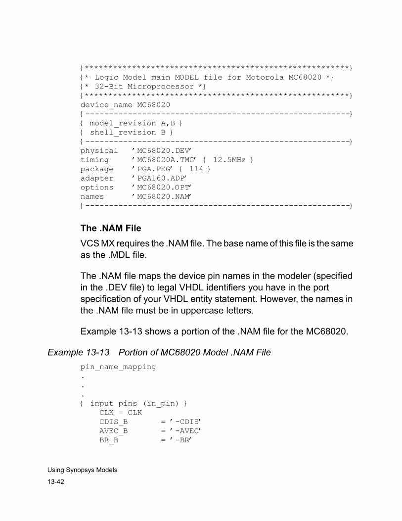
13-42
Using Synopsys Models
{********************************************************}{* Logic Model main MODEL file for Motorola MC68020 *}{* 32-Bit Microprocessor *}{********************************************************}device_name MC68020{--------------------------------------------------------}{ model_revision A,B }{ shell_revision B }{--------------------------------------------------------}physical ’MC68020.DEV’timing ’MC68020A.TMG’ { 12.5MHz }package ’PGA.PKG’ { 114 }adapter ’PGA160.ADP’options ’MC68020.OPT’names ’MC68020.NAM’{--------------------------------------------------------}
The .NAM FileVCS MX requires the .NAM file. The base name of this file is the same as the .MDL file.
The .NAM file maps the device pin names in the modeler (specified in the .DEV file) to legal VHDL identifiers you have in the port specification of your VHDL entity statement. However, the names in the .NAM file must be in uppercase letters.
Example 13-13 shows a portion of the .NAM file for the MC68020.
Example 13-13 Portion of MC68020 Model .NAM Filepin_name_mapping...{ input pins (in_pin) } CLK = CLK CDIS_B = ’-CDIS’ AVEC_B = ’-AVEC’ BR_B = ’-BR’
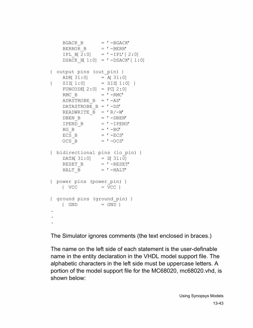
13-43
Using Synopsys Models
BGACK_B = ’-BGACK’ BERROR_B = ’-BERR’ IPL_B[2:0] = ’-IPL’[2:0] DSACK_B[1:0] = ’-DSACK’[1:0]
{ output pins (out_pin) } ADR[31:0] = A[31:0]{ SIZ[1:0] = SIZ[1:0] } FUNCODE[2:0] = FC[2:0] RMC_B = ’-RMC’ ADRSTROBE_B = ’-AS’ DATASTROBE_B = ’-DS’ READWRITE_B = ’R/-W’ DBEN_B = ’-DBEN’ IPEND_B = ’-IPEND’ BG_B = ’-BG’ ECS_B = ’-ECS’ OCS_B = ’-OCS’
{ bidirectional pins (io_pin) } DATA[31:0] = D[31:0] RESET_B = ’-RESET’ HALT_B = ’-HALT’
{ power pins (power_pin) } { VCC = VCC }
{ ground pins (ground_pin) } { GND = GND }...
The Simulator ignores comments (the text enclosed in braces.)
The name on the left side of each statement is the user-definable name in the entity declaration in the VHDL model support file. The alphabetic characters in the left side must be uppercase letters. A portion of the model support file for the MC68020, mc68020.vhd, is shown below:
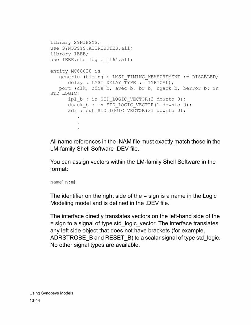
13-44
Using Synopsys Models
library SYNOPSYS;use SYNOPSYS.ATTRIBUTES.all;library IEEE;use IEEE.std_logic_1164.all;
entity MC68020 is generic (timing : LMSI_TIMING_MEASUREMENT := DISABLED; delay : LMSI_DELAY_TYPE := TYPICAL); port (clk, cdis_b, avec_b, br_b, bgack_b, berror_b: in STD_LOGIC; ipl_b : in STD_LOGIC_VECTOR(2 downto 0); dsack_b : in STD_LOGIC_VECTOR(1 downto 0); adr : out STD_LOGIC_VECTOR(31 downto 0);
.
.
.
All name references in the .NAM file must exactly match those in the LM-family Shell Software .DEV file.
You can assign vectors within the LM-family Shell Software in the format:
name[n:m]
The identifier on the right side of the = sign is a name in the Logic Modeling model and is defined in the .DEV file.
The interface directly translates vectors on the left-hand side of the = sign to a signal of type std_logic_vector. The interface translates any left side object that does not have brackets (for example, ADRSTROBE_B and RESET_B) to a scalar signal of type std_logic. No other signal types are available.
13-45
Using Synopsys Models
The order of the port names is not important; however, all pin names you define in the port specification of the VHDL support file must appear in the Shell Software files. Pin names must be in all uppercase letters in the Shell Software files.
The last line in the example mapping CLK to CLK is not required but is included here for clarity. If a name in the .DEV file does not require mapping to another name, it need not appear in the .NAM file.
The .DEV FileThe LM-family modeler requires the .DEV file. The base name of this file is the same as the .MDL file.
Consult the LM-family hardware modeler manual for a list of required and valid file statements. Logic Modeling provides this file with each hardware model so you do not have to modify this file. You do have to view the .DEV file to determine the pin names and pin numbers you must map to the pin names in your VHDL support file. Place this mapping in the .NAM file.
The .DEV file contains statements describing the following physical characteristics of a device:
• Fabrication technology (for example, NMOS)
• Device speed
• Pin I/O characteristics
• Mappings for pin numbers to pin names and device pin numbers to package pin numbers
Example 13-14 shows a portion of the .DEV file for the MC68020 model.
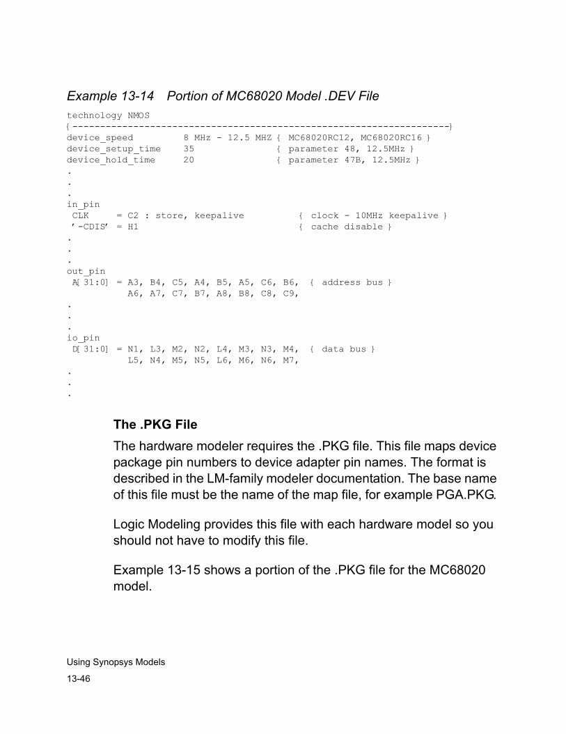
13-46
Using Synopsys Models
Example 13-14 Portion of MC68020 Model .DEV Filetechnology NMOS{--------------------------------------------------------------------}device_speed 8 MHz - 12.5 MHZ { MC68020RC12, MC68020RC16 }device_setup_time 35 { parameter 48, 12.5MHz }device_hold_time 20 { parameter 47B, 12.5MHz }...in_pin CLK = C2 : store, keepalive { clock - 10MHz keepalive } ’-CDIS’ = H1 { cache disable }...out_pin A[31:0] = A3, B4, C5, A4, B5, A5, C6, B6, { address bus } A6, A7, C7, B7, A8, B8, C8, C9,...io_pin D[31:0] = N1, L3, M2, N2, L4, M3, N3, M4, { data bus } L5, N4, M5, N5, L6, M6, N6, M7,...
The .PKG FileThe hardware modeler requires the .PKG file. This file maps device package pin numbers to device adapter pin names. The format is described in the LM-family modeler documentation. The base name of this file must be the name of the map file, for example PGA.PKG.
Logic Modeling provides this file with each hardware model so you should not have to modify this file.
Example 13-15 shows a portion of the .PKG file for the MC68020 model.
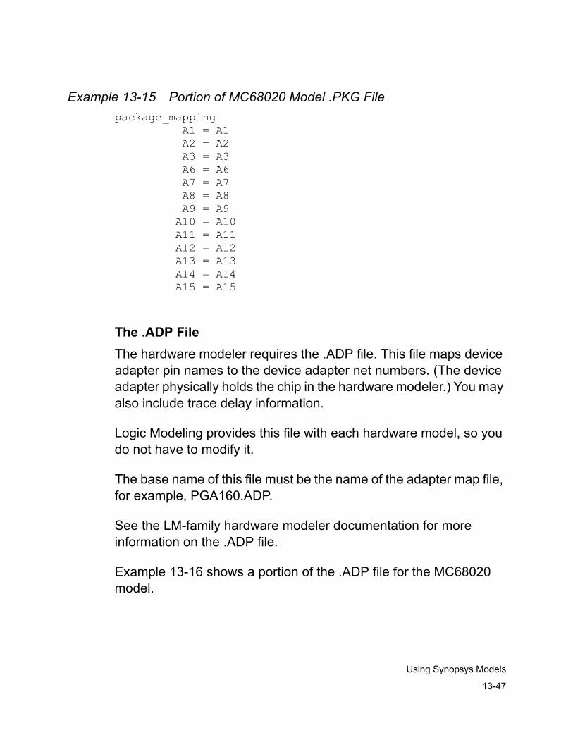
13-47
Using Synopsys Models
Example 13-15 Portion of MC68020 Model .PKG Filepackage_mapping A1 = A1 A2 = A2 A3 = A3 A6 = A6 A7 = A7 A8 = A8 A9 = A9 A10 = A10 A11 = A11 A12 = A12 A13 = A13 A14 = A14 A15 = A15
The .ADP FileThe hardware modeler requires the .ADP file. This file maps device adapter pin names to the device adapter net numbers. (The device adapter physically holds the chip in the hardware modeler.) You may also include trace delay information.
Logic Modeling provides this file with each hardware model, so you do not have to modify it.
The base name of this file must be the name of the adapter map file, for example, PGA160.ADP.
See the LM-family hardware modeler documentation for more information on the .ADP file.
Example 13-16 shows a portion of the .ADP file for the MC68020 model.
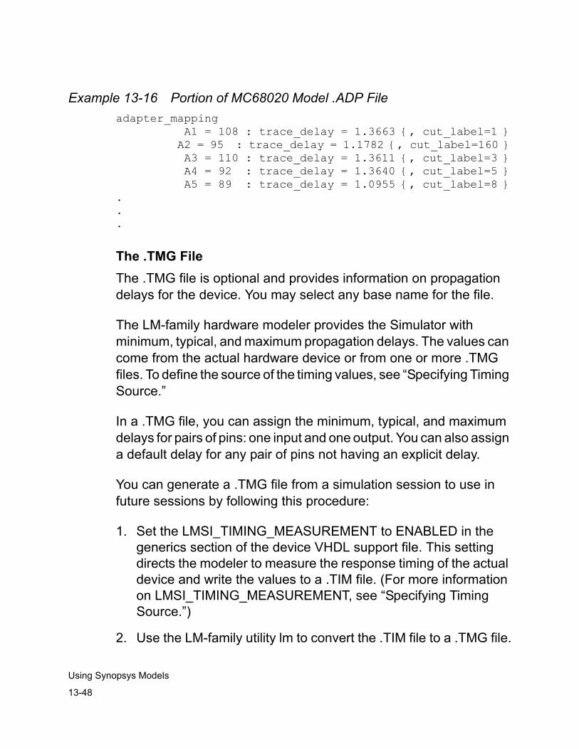
13-48
Using Synopsys Models
Example 13-16 Portion of MC68020 Model .ADP Fileadapter_mapping A1 = 108 : trace_delay = 1.3663 {, cut_label=1 } A2 = 95 : trace_delay = 1.1782 {, cut_label=160 } A3 = 110 : trace_delay = 1.3611 {, cut_label=3 } A4 = 92 : trace_delay = 1.3640 {, cut_label=5 } A5 = 89 : trace_delay = 1.0955 {, cut_label=8 }...
The .TMG FileThe .TMG file is optional and provides information on propagation delays for the device. You may select any base name for the file.
The LM-family hardware modeler provides the Simulator with minimum, typical, and maximum propagation delays. The values can come from the actual hardware device or from one or more .TMG files. To define the source of the timing values, see “Specifying Timing Source.”
In a .TMG file, you can assign the minimum, typical, and maximum delays for pairs of pins: one input and one output. You can also assign a default delay for any pair of pins not having an explicit delay.
You can generate a .TMG file from a simulation session to use in future sessions by following this procedure:
1. Set the LMSI_TIMING_MEASUREMENT to ENABLED in the generics section of the device VHDL support file. This setting directs the modeler to measure the response timing of the actual device and write the values to a .TIM file. (For more information on LMSI_TIMING_MEASUREMENT, see “Specifying Timing Source.”)
2. Use the LM-family utility lm to convert the .TIM file to a .TMG file.
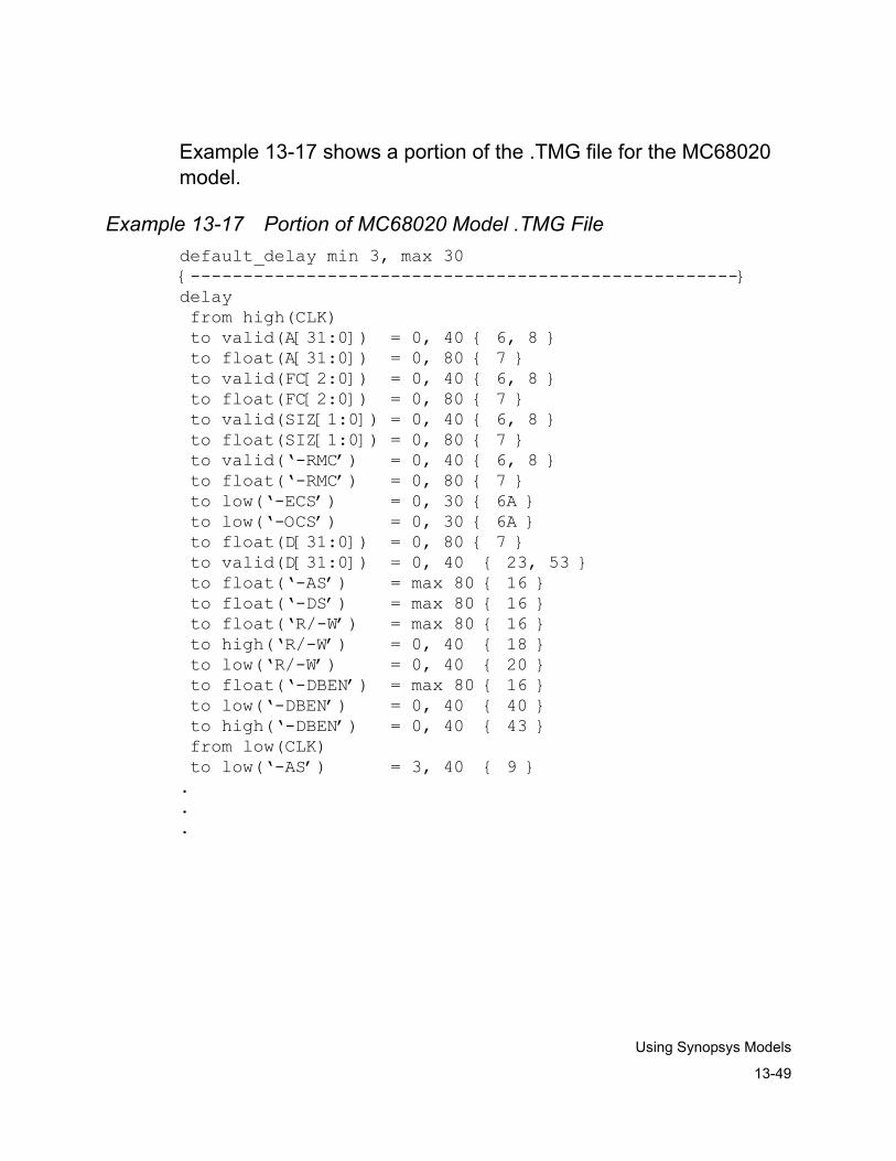
13-49
Using Synopsys Models
Example 13-17 shows a portion of the .TMG file for the MC68020 model.
Example 13-17 Portion of MC68020 Model .TMG Filedefault_delay min 3, max 30{----------------------------------------------------}delay from high(CLK) to valid(A[31:0]) = 0, 40 { 6, 8 } to float(A[31:0]) = 0, 80 { 7 } to valid(FC[2:0]) = 0, 40 { 6, 8 } to float(FC[2:0]) = 0, 80 { 7 } to valid(SIZ[1:0]) = 0, 40 { 6, 8 } to float(SIZ[1:0]) = 0, 80 { 7 } to valid(‘-RMC’) = 0, 40 { 6, 8 } to float(‘-RMC’) = 0, 80 { 7 } to low(‘-ECS’) = 0, 30 { 6A } to low(‘-OCS’) = 0, 30 { 6A } to float(D[31:0]) = 0, 80 { 7 } to valid(D[31:0]) = 0, 40 { 23, 53 } to float(‘-AS’) = max 80 { 16 } to float(‘-DS’) = max 80 { 16 } to float(‘R/-W’) = max 80 { 16 } to high(‘R/-W’) = 0, 40 { 18 } to low(‘R/-W’) = 0, 40 { 20 } to float(‘-DBEN’) = max 80 { 16 } to low(‘-DBEN’) = 0, 40 { 40 } to high(‘-DBEN’) = 0, 40 { 43 } from low(CLK) to low(‘-AS’) = 3, 40 { 9 }...
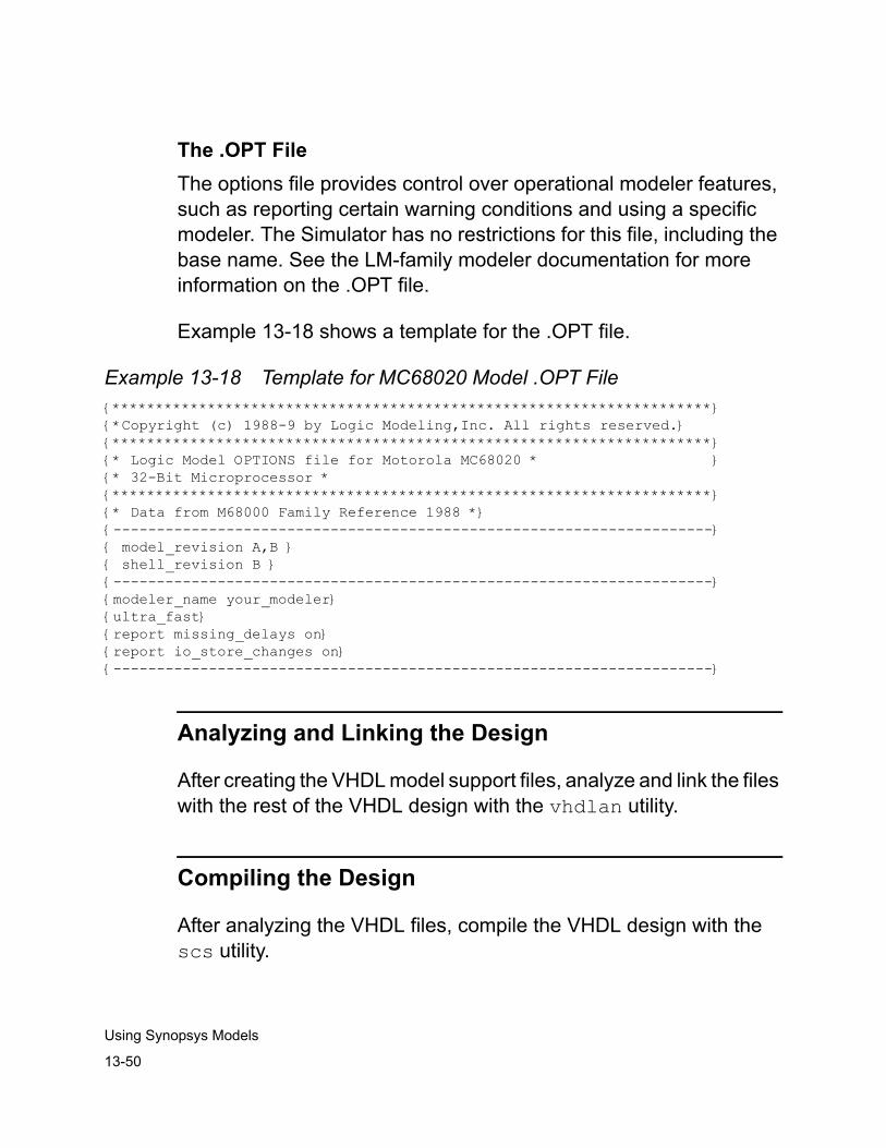
13-50
Using Synopsys Models
The .OPT FileThe options file provides control over operational modeler features, such as reporting certain warning conditions and using a specific modeler. The Simulator has no restrictions for this file, including the base name. See the LM-family modeler documentation for more information on the .OPT file.
Example 13-18 shows a template for the .OPT file.
Example 13-18 Template for MC68020 Model .OPT File{*********************************************************************}{*Copyright (c) 1988-9 by Logic Modeling,Inc. All rights reserved.}{*********************************************************************}{* Logic Model OPTIONS file for Motorola MC68020 * }{* 32-Bit Microprocessor *{*********************************************************************}{* Data from M68000 Family Reference 1988 *}{---------------------------------------------------------------------}{ model_revision A,B }{ shell_revision B }{---------------------------------------------------------------------}{modeler_name your_modeler}{ultra_fast}{report missing_delays on}{report io_store_changes on}{---------------------------------------------------------------------}
Analyzing and Linking the Design
After creating the VHDL model support files, analyze and link the files with the rest of the VHDL design with the vhdlan utility.
Compiling the Design
After analyzing the VHDL files, compile the VHDL design with the scs utility.
13-51
Using Synopsys Models
Simulating the Design
To simulate the design, invoke the Simulator (scsim).
When you simulate your design with the LM-family modeler, you can use all the VCS MX commands for the VHDL portion of the design.
$LMSI Variable
The predefined simulator variable $LMSI equals the number of LM-family modeler device instances in your design. For example, to determine the number of LM-family modeler device instances in the current design, at the Simulator prompt type
# echo $LMSI
Simulator and LM-Family Modeler Interaction
A simulation session with LM-family models has several steps:
• Initialization
• Instantiation
• Multiple evaluations
• Release of the hardware modeler
These steps are transparent to the user and are only provided here for you to understand how the VHDL Simulator and LM-family modeler operate together.
13-52
Using Synopsys Models
Initialization
The Simulator does not initialize an LM-family model until it needs to instantiate the device in the simulation. This avoids time-consuming interaction with the modeler.
The host system, Simulator, and modeler perform the following steps at initialization:
• The host system (for example, Sun) environment provides the hostname and username to initialize an LM-family model. If the host system environment does not provide hostname and username, the default value for both of these is vhdl.
• VCS MX provides the modeler with the base simulation time unit. The TIMEBASE setup variable in the synopsys_sim.setup file normally defines this value; the default value is NS (nanoseconds.) However, you can set the base simulation time unit on VCS MX compiler (scs) invocation command line with the -time option.
• The modeler converts all user-specified LM-family Shell Software delays to the equivalent number of simulation ticks. The modeler internally resolves all timing information to units of 1 picosecond.
• The Simulator performs the mapping between std_logic and the modeler logic values at initialization time. There are no weak-X, undefined, or don’t-care (‘W’, ‘U’, and ‘-’, respectively) equivalent to the IEEE 1164 values in the LM-family modeler. The Simulator maps these three logic values to ‘X’ in the STD_LOGIC value set.
13-53
Using Synopsys Models
Instantiation
During the Simulator (scsim) instantiation phase, the Simulator first defines then instantiates the device. Your design can contain multiple instantiations of a single physical hardware device. Instantiation requires that the host system environment provide the following information:
• Name of the modeler assigned to the modeling session if two or more modelers are on the network. The name is in the Shell Software files.
• Name of the device found in the .MDL Shell file that you use as the entity name in your VHDL design.
The LM-family modeler must physically contain the hardware model, or the instantiation fails.
Evaluation
When the Simulator (scsim) determines that it has changed an input to an instance of a device in the modeler, it begins the evaluation process with the modeler.
For each model evaluation, VCS MX
1. Transmits each pin number and its associated new value to the modeler.
2. Calls the modeler to get the value of each pin whose output has subsequently changed.
13-54
Using Synopsys Models
The modeler returns the information for each pin including pin type, value, and the minimum, typical, and maximum delay values. You can assign the delay value you want VCS MX to use in the generic entity declaration. For more information, see the “Specifying Timing Source and Delay Type” section.
Release of Resources
At the end of simulation, VCS MX releases all host and modeler resources and ends the modeling sessions. However, in the case of an abnormal end to the simulator (for example, the host machine crashes while VCS MX is running), the LM-family modeler does not clear out its instance data. In this case, use the LM-family utility lm to clear any invalid or old information. See the LM-family modeler documentation for a description of this utility.
Error Messages
The Simulator receives error messages from the LM-family modeler and formats them according to Synopsys’ standard error reporting syntax:
SEVERITY_LEVEL: scsim[,error_number]: From the Logic Modeling Logic Model Interface: LM_error_message
SEVERITY_LEVELErrors originating in the LM-family modeler or in associated files generate error messages with two levels of severity: error and warning. The two are described below:
**ErrorThe modeling session cannot continue, but the Simulator is still running.
Warning
13-55
Using Synopsys Models
The modeling session can continue, but an error could occur later in the simulation session.
[error_number]Internal error number.
LM_error_messageThis is the message generated by the modeler. These messages use four different formats that identify the source of the error:
filename, line: messageThe error is from the LM-family Software Shell.
message_onlyThe error is from the operation of the modeler.
internal simulator error: messageThe error is from internal communications.
internal error: messageThe error is from internal hardware or software.
The following example is an error message from VCS MX and the modeler:
**Error: scsim,131: From the Logic Modeling Logic Model Interface: unable to find file
The next example is a warning from VCS MX and the modeler:
Warning: scsim,130: From the Logic Modeling Logic Model Interface: Unable to open directory for reading: /usr/synopsys/sparcOS5/sim/lm1000/models
13-56
Using Synopsys Models
LM-Family Modeler Example
This example uses Synopsys’s LM-1000 modeler and MC68020 microprocessor Logic Model. In this simulation, the Motorola MC68020 microprocessor runs a compiled C program that generates the first numbers of the Fibonacci series.
To run the simulation, you need Synopsys’s Logic Model for the MC68020. If you do not have this model, you may still find it worthwhile to read through the example to understand the procedures used with the modeler.
You need two kinds of files to support the simulation by using the modeler:
• VHDL model support files.
A VHDL model support file for this example (which you usually provide) is in $VCS_HOME/doc/sim/examples/lmsi_if.
• LM-family Shell Software files.
Synopsys provides the LM-family Shell Software files with the LM-family Logic Model.
Figure 13-2 shows the MC68020 chip and its related processes. These processes, implemented in software on the Simulator, represent the supporting circuitry of the MC68020.
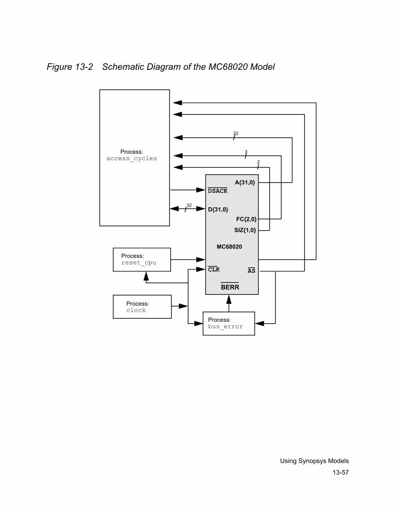
13-57
Using Synopsys Models
Figure 13-2 Schematic Diagram of the MC68020 Model
Process:clock
32/
3/
2/
Process:access_cycles
Process:bus_error
Process:reset_cpu
MC6802
32 /
A{31,0}DSACK
D{31,0} FC{2,0}
SIZ{1,0}
CLK
AS
BERR
MC68020
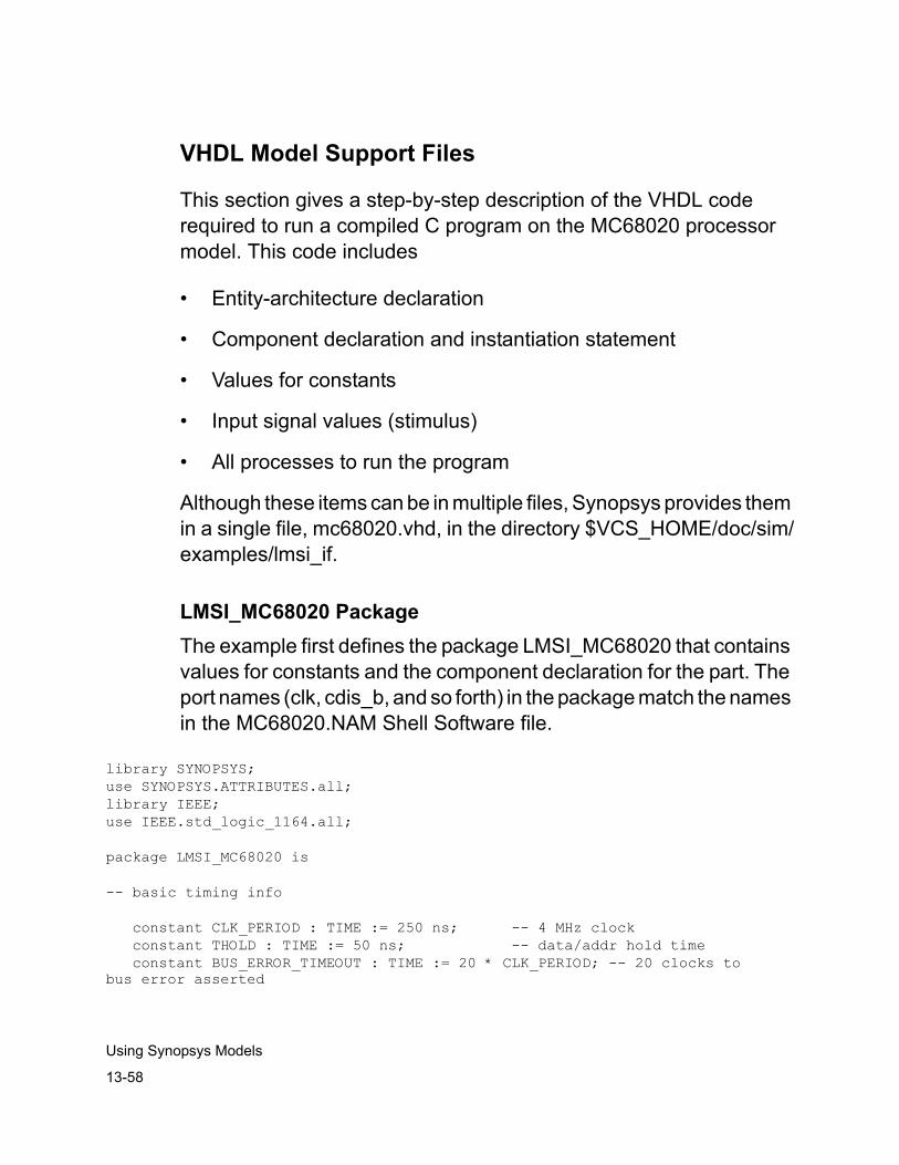
13-58
Using Synopsys Models
VHDL Model Support Files
This section gives a step-by-step description of the VHDL code required to run a compiled C program on the MC68020 processor model. This code includes
• Entity-architecture declaration
• Component declaration and instantiation statement
• Values for constants
• Input signal values (stimulus)
• All processes to run the program
Although these items can be in multiple files, Synopsys provides them in a single file, mc68020.vhd, in the directory $VCS_HOME/doc/sim/examples/lmsi_if.
LMSI_MC68020 PackageThe example first defines the package LMSI_MC68020 that contains values for constants and the component declaration for the part. The port names (clk, cdis_b, and so forth) in the package match the names in the MC68020.NAM Shell Software file.
library SYNOPSYS;use SYNOPSYS.ATTRIBUTES.all;library IEEE;use IEEE.std_logic_1164.all;
package LMSI_MC68020 is
-- basic timing info
constant CLK_PERIOD : TIME := 250 ns; -- 4 MHz clock constant THOLD : TIME := 50 ns; -- data/addr hold time constant BUS_ERROR_TIMEOUT : TIME := 20 * CLK_PERIOD; -- 20 clocks tobus error asserted
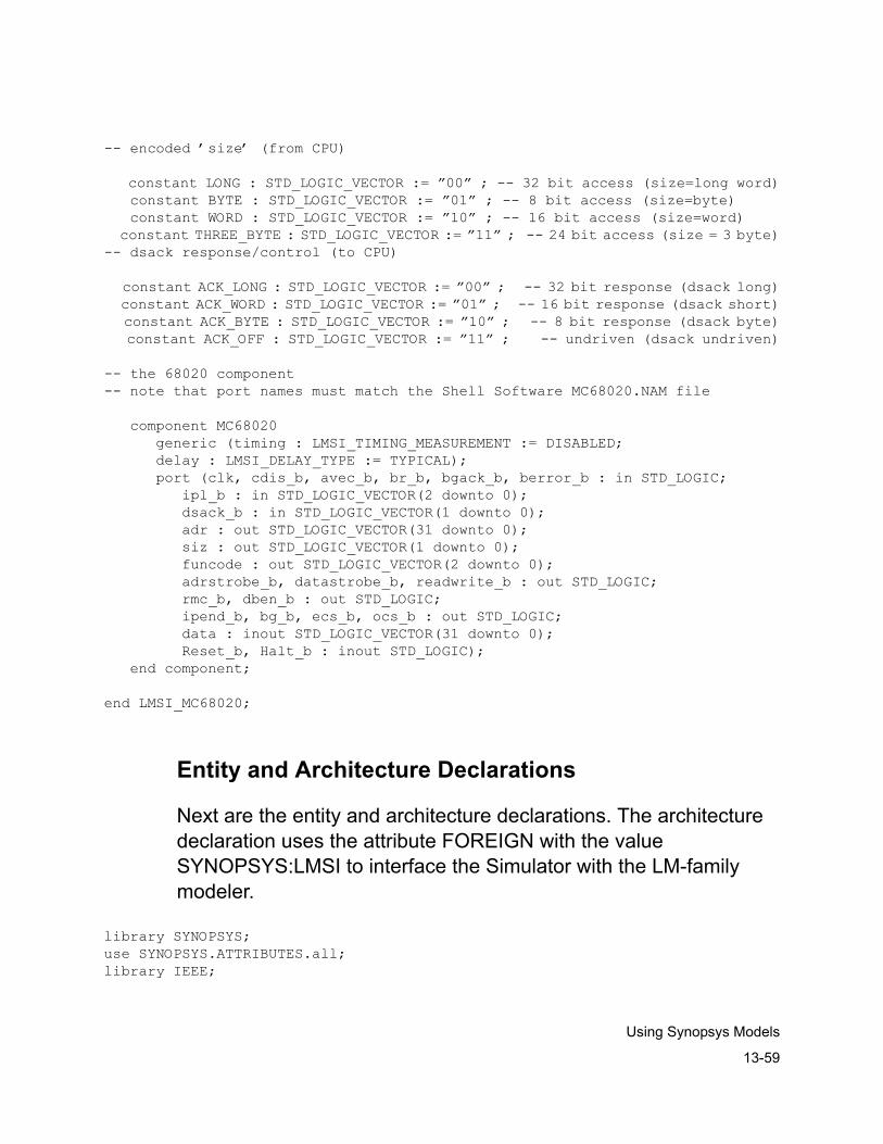
13-59
Using Synopsys Models
-- encoded ’size’ (from CPU)
constant LONG : STD_LOGIC_VECTOR := ”00” ; -- 32 bit access (size=long word) constant BYTE : STD_LOGIC_VECTOR := ”01” ; -- 8 bit access (size=byte) constant WORD : STD_LOGIC_VECTOR := ”10” ; -- 16 bit access (size=word) constant THREE_BYTE : STD_LOGIC_VECTOR := ”11” ; -- 24 bit access (size = 3 byte)-- dsack response/control (to CPU)
constant ACK_LONG : STD_LOGIC_VECTOR := ”00” ; -- 32 bit response (dsack long) constant ACK_WORD : STD_LOGIC_VECTOR := ”01” ; -- 16 bit response (dsack short) constant ACK_BYTE : STD_LOGIC_VECTOR := ”10” ; -- 8 bit response (dsack byte) constant ACK_OFF : STD_LOGIC_VECTOR := ”11” ; -- undriven (dsack undriven)
-- the 68020 component-- note that port names must match the Shell Software MC68020.NAM file
component MC68020 generic (timing : LMSI_TIMING_MEASUREMENT := DISABLED; delay : LMSI_DELAY_TYPE := TYPICAL); port (clk, cdis_b, avec_b, br_b, bgack_b, berror_b : in STD_LOGIC; ipl_b : in STD_LOGIC_VECTOR(2 downto 0); dsack_b : in STD_LOGIC_VECTOR(1 downto 0); adr : out STD_LOGIC_VECTOR(31 downto 0); siz : out STD_LOGIC_VECTOR(1 downto 0); funcode : out STD_LOGIC_VECTOR(2 downto 0); adrstrobe_b, datastrobe_b, readwrite_b : out STD_LOGIC; rmc_b, dben_b : out STD_LOGIC; ipend_b, bg_b, ecs_b, ocs_b : out STD_LOGIC; data : inout STD_LOGIC_VECTOR(31 downto 0); Reset_b, Halt_b : inout STD_LOGIC); end component;
end LMSI_MC68020;
Entity and Architecture Declarations
Next are the entity and architecture declarations. The architecture declaration uses the attribute FOREIGN with the value SYNOPSYS:LMSI to interface the Simulator with the LM-family modeler.
library SYNOPSYS;use SYNOPSYS.ATTRIBUTES.all;library IEEE;
13-60
Using Synopsys Models
use IEEE.std_logic_1164.all;
entity MC68020 is generic (timing : LMSI_TIMING_MEASUREMENT := DISABLED; delay : LMSI_DELAY_TYPE := TYPICAL); port (clk, cdis_b, avec_b, br_b, bgack_b, berror_b : in STD_LOGIC; ipl_b : in STD_LOGIC_VECTOR(2 downto 0); dsack_b : in STD_LOGIC_VECTOR(1 downto 0); adr : out STD_LOGIC_VECTOR(31 downto 0); siz : out STD_LOGIC_VECTOR(1 downto 0); funcode : out STD_LOGIC_VECTOR(2 downto 0); adrstrobe_b, datastrobe_b, readwrite_b : out STD_LOGIC; rmc_b, dben_b : out STD_LOGIC; ipend_b, bg_b, ecs_b, ocs_b : out STD_LOGIC; data : inout STD_LOGIC_VECTOR(31 downto 0); Reset_b, Halt_b : inout STD_LOGIC);end MC68020;
library SYNOPSYS;use SYNOPSYS.ATTRIBUTES.all;architecture LMSI of MC68020 is attribute FOREIGN of LMSI : architecture is “SYNOPSYS:LMSI”;beginend;
Component Instantiation and Input StimulusThe last code is the testbench. It instantiates the component U0 and declares its input signals with initial values and output signals. Processes provide the input stimulus that mimic the support circuitry of the microprocessor.
The top-level entity is empty. The first portion of the architecture defines the initial values of all the in and inout ports.
library SYNOPSYS;use SYNOPSYS.ATTRIBUTES.all;use SYNOPSYS.BV_ARITHMETIC.all;library IEEE;use IEEE.std_logic_1164.all;use IEEE.std_logic_arith.all;use WORK.LMSI_MC68020.all;
entity E isend E;
13-61
Using Synopsys Models
architecture A of E is
-- inputs signal clk : STD_LOGIC := ’0’ ; -- start off clock low signal reset : STD_LOGIC := ’L’ ; -- start off in reset mode signal halt : STD_LOGIC := ’H’ ; -- ... with reset on, no halt signal dsack : STD_LOGIC_VECTOR(1 downto 0) := ACK_OFF; -- data strobe ack (start ’OFF’) signal data : STD_LOGIC_VECTOR(31 downto 0):=(others => ’Z’);--data bus
-- outputs signal as : STD_LOGIC; -- address strobe signal ds : STD_LOGIC; -- data strobe signal rw : STD_LOGIC; -- read/write state (read = 1) signal addr : STD_LOGIC_VECTOR(31 downto 0); -- address bus signal size : STD_LOGIC_VECTOR(1 downto 0); -- cycle size
-- unused inputs signal cdis : STD_LOGIC := ’L’ ; -- internal cache disabled signal avec : STD_LOGIC := ’H’ ; -- no autovectors here! signal berr : STD_LOGIC := ’H’ ; -- ... or bus errors signal br : STD_LOGIC := ’H’ ; -- ... or bus requests signal bgack : STD_LOGIC := ’H’ ; -- ... or bus grants signal ipl : STD_LOGIC_VECTOR(2 downto 0) := (others => ’H’); --level 0
-- unused outputs signal bg : STD_LOGIC; -- bus grant (n/u) signal ecs,ocs : STD_LOGIC; -- ext/op cycle start (n/u) signal rmc : STD_LOGIC; -- read/mod/write cycle (n/u) signal dben : STD_LOGIC := ’H’; -- data bus enabled (n/u) signal funcode :STD_LOGIC_VECTOR(2 downto 0);--process state info (n/u) signal ipend : STD_LOGIC; -- interrupt pending (n/u)
for all : WORK.LMSI_MC68020.MC68020 use entity WORK.MC68020(LMSI); begin
U0 : WORK.LMSI_MC68020.MC68020 generic map (ENABLED, MAXIMUM) port map ( clk => clk, cdis_b => cdis, avec_b => avec, br_b => br, bgack_b => bgack, berror_b => berr, ipl_b => ipl, dsack_b => dsack, adr => addr, siz => size, funcode => funcode, rmc_b => rmc, adrstrobe_b => as, datastrobe_b => ds, readwrite_b => rw, dben_b => dben, ipend_b => ipend, bg_b => bg, ecs_b => ecs, ocs_b => ocs, data => data, reset_b => reset, halt_b => halt);
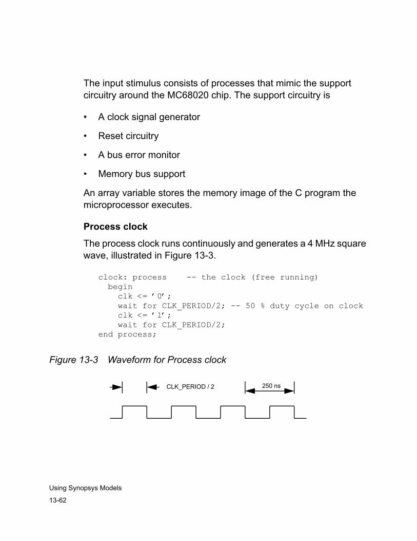
13-62
Using Synopsys Models
The input stimulus consists of processes that mimic the support circuitry around the MC68020 chip. The support circuitry is
• A clock signal generator
• Reset circuitry
• A bus error monitor
• Memory bus support
An array variable stores the memory image of the C program the microprocessor executes.
Process clock
The process clock runs continuously and generates a 4 MHz square wave, illustrated in Figure 13-3.
clock: process -- the clock (free running) begin clk <= ’0’; wait for CLK_PERIOD/2; -- 50 % duty cycle on clock clk <= ’1’; wait for CLK_PERIOD/2; end process;
Figure 13-3 Waveform for Process clock
CLK_PERIOD / 2 250 ns
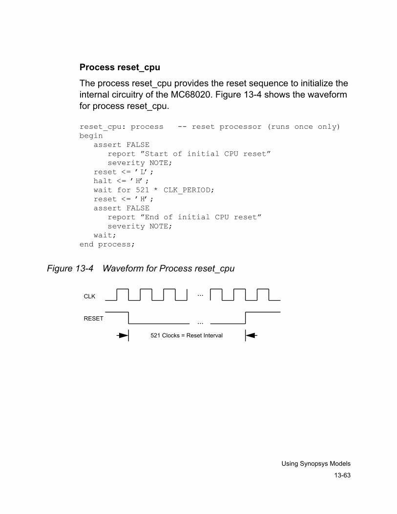
13-63
Using Synopsys Models
Process reset_cpu
The process reset_cpu provides the reset sequence to initialize the internal circuitry of the MC68020. Figure 13-4 shows the waveform for process reset_cpu.
reset_cpu: process -- reset processor (runs once only)begin assert FALSE report ”Start of initial CPU reset” severity NOTE; reset <= ’L’; halt <= ’H’; wait for 521 * CLK_PERIOD; reset <= ’H’; assert FALSE report ”End of initial CPU reset” severity NOTE; wait;end process;
Figure 13-4 Waveform for Process reset_cpu
CLK
RESET
521 Clocks = Reset Interval
...
...
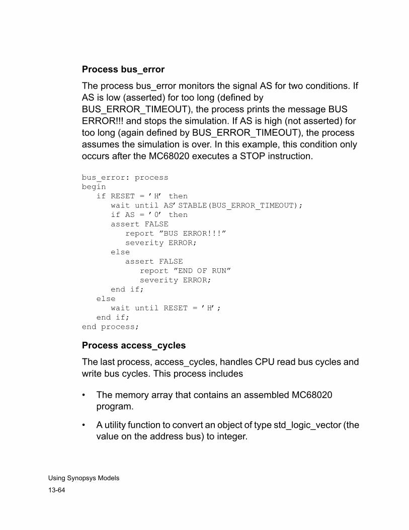
13-64
Using Synopsys Models
Process bus_error
The process bus_error monitors the signal AS for two conditions. If AS is low (asserted) for too long (defined by BUS_ERROR_TIMEOUT), the process prints the message BUS ERROR!!! and stops the simulation. If AS is high (not asserted) for too long (again defined by BUS_ERROR_TIMEOUT), the process assumes the simulation is over. In this example, this condition only occurs after the MC68020 executes a STOP instruction.
bus_error: processbegin if RESET = ’H’ then wait until AS’STABLE(BUS_ERROR_TIMEOUT); if AS = ’0’ then assert FALSE report ”BUS ERROR!!!” severity ERROR; else assert FALSE report ”END OF RUN” severity ERROR; end if; else wait until RESET = ’H’; end if;end process;
Process access_cycles
The last process, access_cycles, handles CPU read bus cycles and write bus cycles. This process includes
• The memory array that contains an assembled MC68020 program.
• A utility function to convert an object of type std_logic_vector (the value on the address bus) to integer.
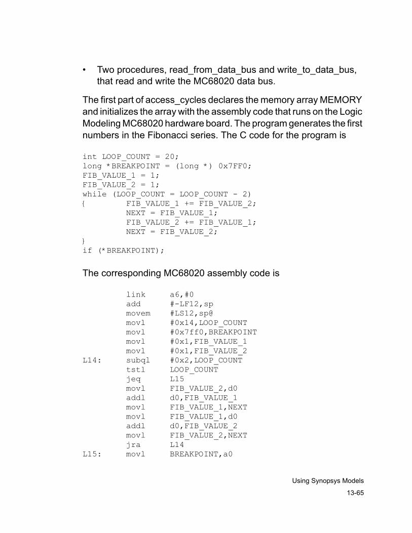
13-65
Using Synopsys Models
• Two procedures, read_from_data_bus and write_to_data_bus, that read and write the MC68020 data bus.
The first part of access_cycles declares the memory array MEMORY and initializes the array with the assembly code that runs on the Logic Modeling MC68020 hardware board. The program generates the first numbers in the Fibonacci series. The C code for the program is
int LOOP_COUNT = 20;long *BREAKPOINT = (long *) 0x7FF0;FIB_VALUE_1 = 1;FIB_VALUE_2 = 1;while (LOOP_COUNT = LOOP_COUNT - 2){ FIB_VALUE_1 += FIB_VALUE_2; NEXT = FIB_VALUE_1; FIB_VALUE_2 += FIB_VALUE_1; NEXT = FIB_VALUE_2;}if (*BREAKPOINT);
The corresponding MC68020 assembly code is
link a6,#0 add #-LF12,sp movem #LS12,sp@ movl #0x14,LOOP_COUNT movl #0x7ff0,BREAKPOINT movl #0x1,FIB_VALUE_1 movl #0x1,FIB_VALUE_2L14: subql #0x2,LOOP_COUNT tstl LOOP_COUNT jeq L15 movl FIB_VALUE_2,d0 addl d0,FIB_VALUE_1 movl FIB_VALUE_1,NEXT movl FIB_VALUE_1,d0 addl d0,FIB_VALUE_2 movl FIB_VALUE_2,NEXT jra L14L15: movl BREAKPOINT,a0
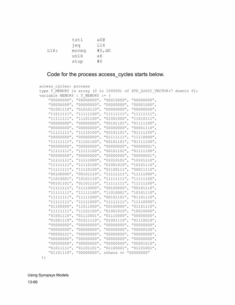
13-66
Using Synopsys Models
tstl a0@ jeq L16L16: moveq #0,d0 unlk a6 stop #0
Code for the process access_cycles starts below.
access_cycles: process type T_MEMORY is array (0 to 100000) of STD_LOGIC_VECTOR(7 downto 0); variable MEMORY : T_MEMORY := ( ”00000000”, ”00000000”, ”00010000”, ”00000000”, ”00000000”, ”00000000”, ”00000000”, ”00001000”, ”01001110”, ”01010110”, ”00000000”, ”00000000”, ”11011111”, ”11111100”, ”11111111”, ”11111111”, ”11111111”, ”11101100”, ”01001000”, ”11010111”, ”00000000”, ”00000000”, ”00101101”, ”01111100”, ”00000000”, ”00000000”, ”00000000”, ”00001110”, ”11111111”, ”11110100”, ”00101101”, ”01111100”, ”00000000”, ”00000000”, ”01111111”, ”11110000”, ”11111111”, ”11101100”, ”00101101”, ”01111100”, ”00000000”, ”00000000”, ”00000000”, ”00000001”, ”11111111”, ”11111100”, ”00101101”, ”01111100”, ”00000000”, ”00000000”, ”00000000”, ”00000001”, ”11111111”, ”11111000”, ”01010101”, ”10101110”, ”11111111”, ”11110100”, ”01001010”, ”10101110”, ”11111111”, ”11110100”, ”01100111”, ”00011110”, ”00100000”, ”00101110”, ”11111111”, ”11111000”, ”11010001”, ”10101110”, ”11111111”, ”11111100”, ”00101101”, ”01101110”, ”11111111”, ”11111100”, ”11111111”, ”11110000”, ”00100000”, ”00101110”, ”11111111”, ”11111100”, ”11010001”, ”10101110”, ”11111111”, ”11111000”, ”00101101”, ”01101110”, ”11111111”, ”11111000”, ”11111111”, ”11110000”, ”01100000”, ”11011000”, ”00100000”, ”01101110”, ”11111111”, ”11101100”, ”01001010”, ”10010000”, ”01001110”, ”01110001”, ”01110000”, ”00000000”, ”01001110”, ”01011110”, ”01001110”, ”01110010”, ”00000000”, ”00000000”, ”00000000”, ”00000000”, ”00000000”, ”00000000”, ”00000000”, ”00000100”, ”00000101”, ”00000000”, ”00000000”, ”00000000”, ”00000000”, ”00000000”, ”00000000”, ”00000000”, ”00000000”, ”00000000”, ”00000000”, ”00001010”, ”01011111”, ”01101101”, ”01100001”, ”01101001”, ”01101110”, ”00000000”, others => ”00000000” );
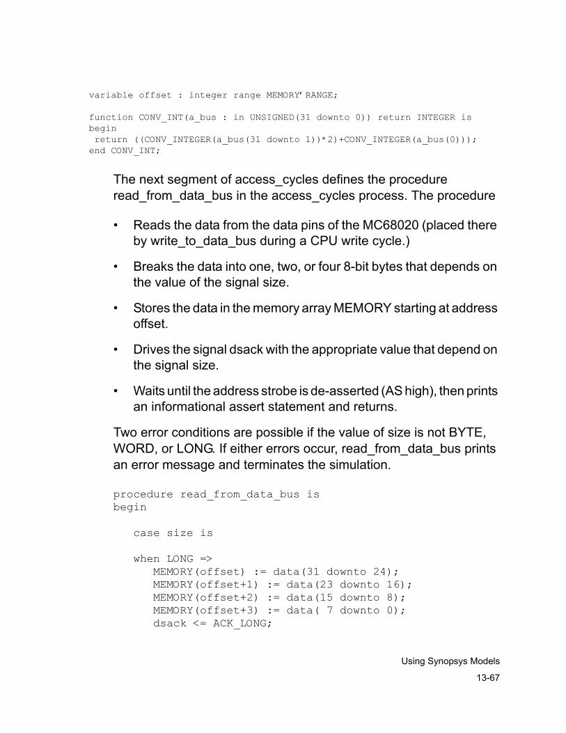
13-67
Using Synopsys Models
variable offset : integer range MEMORY’RANGE;
function CONV_INT(a_bus : in UNSIGNED(31 downto 0)) return INTEGER is begin return ((CONV_INTEGER(a_bus(31 downto 1))*2)+CONV_INTEGER(a_bus(0))); end CONV_INT;
The next segment of access_cycles defines the procedure read_from_data_bus in the access_cycles process. The procedure
• Reads the data from the data pins of the MC68020 (placed there by write_to_data_bus during a CPU write cycle.)
• Breaks the data into one, two, or four 8-bit bytes that depends on the value of the signal size.
• Stores the data in the memory array MEMORY starting at address offset.
• Drives the signal dsack with the appropriate value that depend on the signal size.
• Waits until the address strobe is de-asserted (AS high), then prints an informational assert statement and returns.
Two error conditions are possible if the value of size is not BYTE, WORD, or LONG. If either errors occur, read_from_data_bus prints an error message and terminates the simulation.
procedure read_from_data_bus isbegin
case size is
when LONG => MEMORY(offset) := data(31 downto 24); MEMORY(offset+1) := data(23 downto 16); MEMORY(offset+2) := data(15 downto 8); MEMORY(offset+3) := data( 7 downto 0); dsack <= ACK_LONG;
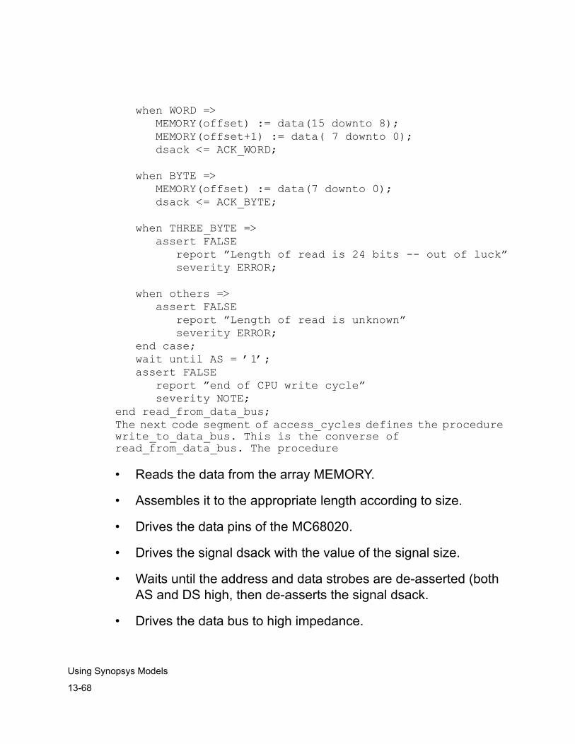
13-68
Using Synopsys Models
when WORD => MEMORY(offset) := data(15 downto 8); MEMORY(offset+1) := data( 7 downto 0); dsack <= ACK_WORD;
when BYTE => MEMORY(offset) := data(7 downto 0); dsack <= ACK_BYTE;
when THREE_BYTE => assert FALSE report ”Length of read is 24 bits -- out of luck” severity ERROR;
when others => assert FALSE report ”Length of read is unknown” severity ERROR; end case; wait until AS = ’1’; assert FALSE report ”end of CPU write cycle” severity NOTE;end read_from_data_bus;The next code segment of access_cycles defines the procedure write_to_data_bus. This is the converse of read_from_data_bus. The procedure
• Reads the data from the array MEMORY.
• Assembles it to the appropriate length according to size.
• Drives the data pins of the MC68020.
• Drives the signal dsack with the value of the signal size.
• Waits until the address and data strobes are de-asserted (both AS and DS high, then de-asserts the signal dsack.
• Drives the data bus to high impedance.
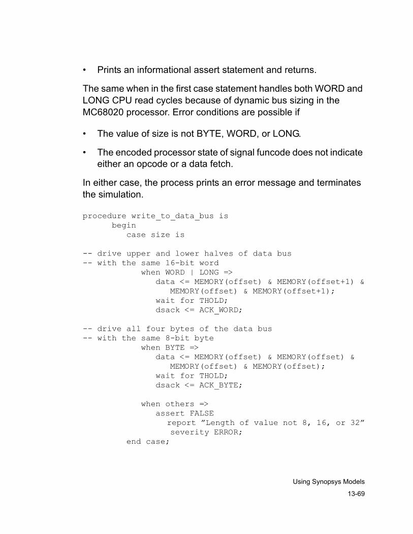
13-69
Using Synopsys Models
• Prints an informational assert statement and returns.
The same when in the first case statement handles both WORD and LONG CPU read cycles because of dynamic bus sizing in the MC68020 processor. Error conditions are possible if
• The value of size is not BYTE, WORD, or LONG.
• The encoded processor state of signal funcode does not indicate either an opcode or a data fetch.
In either case, the process prints an error message and terminates the simulation.
procedure write_to_data_bus is begin case size is
-- drive upper and lower halves of data bus-- with the same 16-bit word when WORD | LONG => data <= MEMORY(offset) & MEMORY(offset+1) & MEMORY(offset) & MEMORY(offset+1); wait for THOLD; dsack <= ACK_WORD;
-- drive all four bytes of the data bus-- with the same 8-bit byte when BYTE => data <= MEMORY(offset) & MEMORY(offset) & MEMORY(offset) & MEMORY(offset); wait for THOLD; dsack <= ACK_BYTE;
when others => assert FALSE report ”Length of value not 8, 16, or 32” severity ERROR; end case;
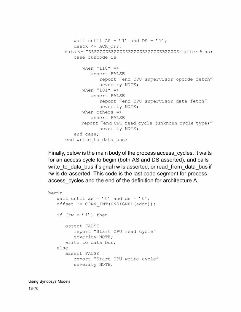
13-70
Using Synopsys Models
wait until AS = ’1’ and DS = ’1’; dsack <= ACK_OFF; data <= ”ZZZZZZZZZZZZZZZZZZZZZZZZZZZZZZZZ” after 5 ns; case funcode is
when ”110” => assert FALSE report ”end CPU supervisor opcode fetch” severity NOTE; when ”101” => assert FALSE report ”end CPU supervisor data fetch” severity NOTE; when others => assert FALSE report ”end CPU read cycle (unknown cycle type)” severity NOTE; end case; end write_to_data_bus;
Finally, below is the main body of the process access_cycles. It waits for an access cycle to begin (both AS and DS asserted), and calls write_to_data_bus if signal rw is asserted, or read_from_data_bus if rw is de-asserted. This code is the last code segment for process access_cycles and the end of the definition for architecture A.
begin wait until as = ’0’ and ds = ’0’; offset := CONV_INT(UNSIGNED(addr));
if (rw = ’1’) then
assert FALSE report ”Start CPU read cycle” severity NOTE; write_to_data_bus; else assert FALSE report ”Start CPU write cycle” severity NOTE;
13-71
Using Synopsys Models
read_from_data_bus; end if;
end process;end;
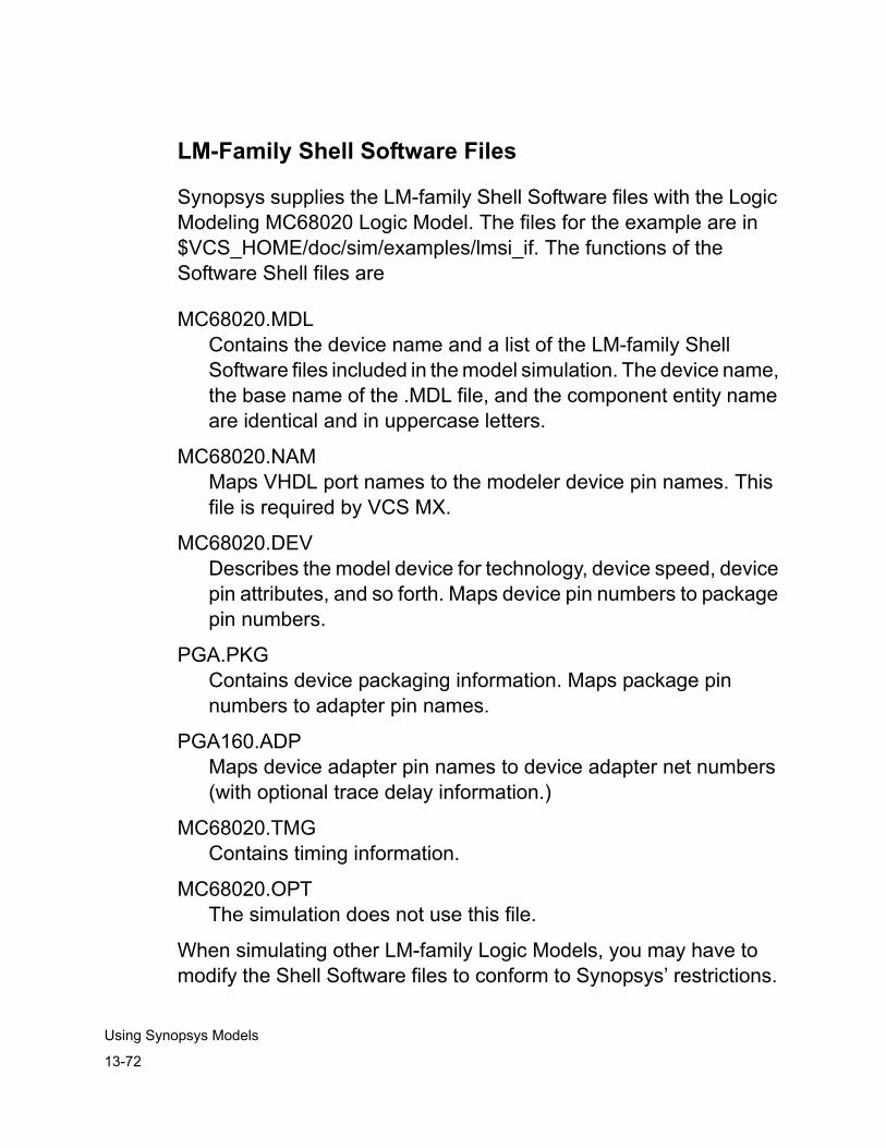
13-72
Using Synopsys Models
LM-Family Shell Software Files
Synopsys supplies the LM-family Shell Software files with the Logic Modeling MC68020 Logic Model. The files for the example are in $VCS_HOME/doc/sim/examples/lmsi_if. The functions of the Software Shell files are
MC68020.MDLContains the device name and a list of the LM-family Shell Software files included in the model simulation. The device name, the base name of the .MDL file, and the component entity name are identical and in uppercase letters.
MC68020.NAMMaps VHDL port names to the modeler device pin names. This file is required by VCS MX.
MC68020.DEVDescribes the model device for technology, device speed, device pin attributes, and so forth. Maps device pin numbers to package pin numbers.
PGA.PKGContains device packaging information. Maps package pin numbers to adapter pin names.
PGA160.ADPMaps device adapter pin names to device adapter net numbers (with optional trace delay information.)
MC68020.TMGContains timing information.
MC68020.OPTThe simulation does not use this file.
When simulating other LM-family Logic Models, you may have to modify the Shell Software files to conform to Synopsys’ restrictions.
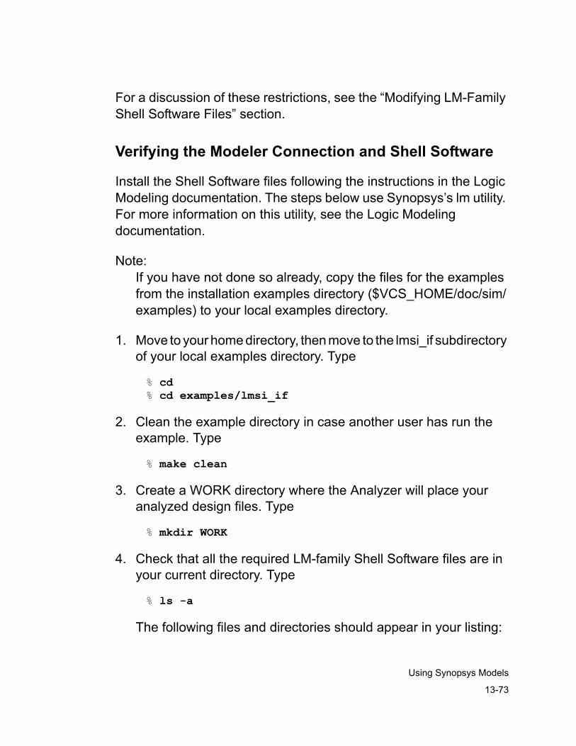
13-73
Using Synopsys Models
For a discussion of these restrictions, see the “Modifying LM-Family Shell Software Files” section.
Verifying the Modeler Connection and Shell Software
Install the Shell Software files following the instructions in the Logic Modeling documentation. The steps below use Synopsys’s lm utility. For more information on this utility, see the Logic Modeling documentation.
Note:If you have not done so already, copy the files for the examples from the installation examples directory ($VCS_HOME/doc/sim/examples) to your local examples directory.
1. Move to your home directory, then move to the lmsi_if subdirectory of your local examples directory. Type
% cd% cd examples/lmsi_if
2. Clean the example directory in case another user has run the example. Type
% make clean
3. Create a WORK directory where the Analyzer will place your analyzed design files. Type
% mkdir WORK
4. Check that all the required LM-family Shell Software files are in your current directory. Type
% ls -a
The following files and directories should appear in your listing:
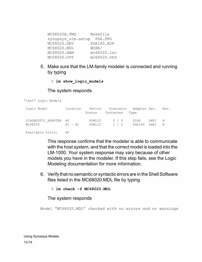
13-74
Using Synopsys Models
MC68020A.TMG Makefilesynopsys_sim.setup PGA.PKGMC68020.DEV PGA160.ADPMC68020.MDL WORK/MC68020.NAM mc68020.incMC68020.OPT mc68020.vhd
5. Make sure that the LM-family modeler is connected and running by typing
% lm show_logic_models
The system responds
”lmsi” Logic Models
Logic Model Location Device Simulator Adapter Dev. Rev. Status Instances Type
DIAGNOSTIC_ADAPTER A0 PUBLIC 0 / 0 DIAG LMSI A MC68020 A1 - B1 PUBLIC 1 / 0 PGA160 LMSI B
Available Slots: B0
This response confirms that the modeler is able to communicate with the host system, and that the correct model is loaded into the LM-1000. Your system response may vary because of other models you have in the modeler. If this step fails, see the Logic Modeling documentation for more information.
6. Verify that no semantic or syntactic errors are in the Shell Software files listed in the MC68020.MDL file by typing
% lm check -f MC68020.MDL
The system responds
Model ”MC68020.MDL” checked with no errors and no warnings
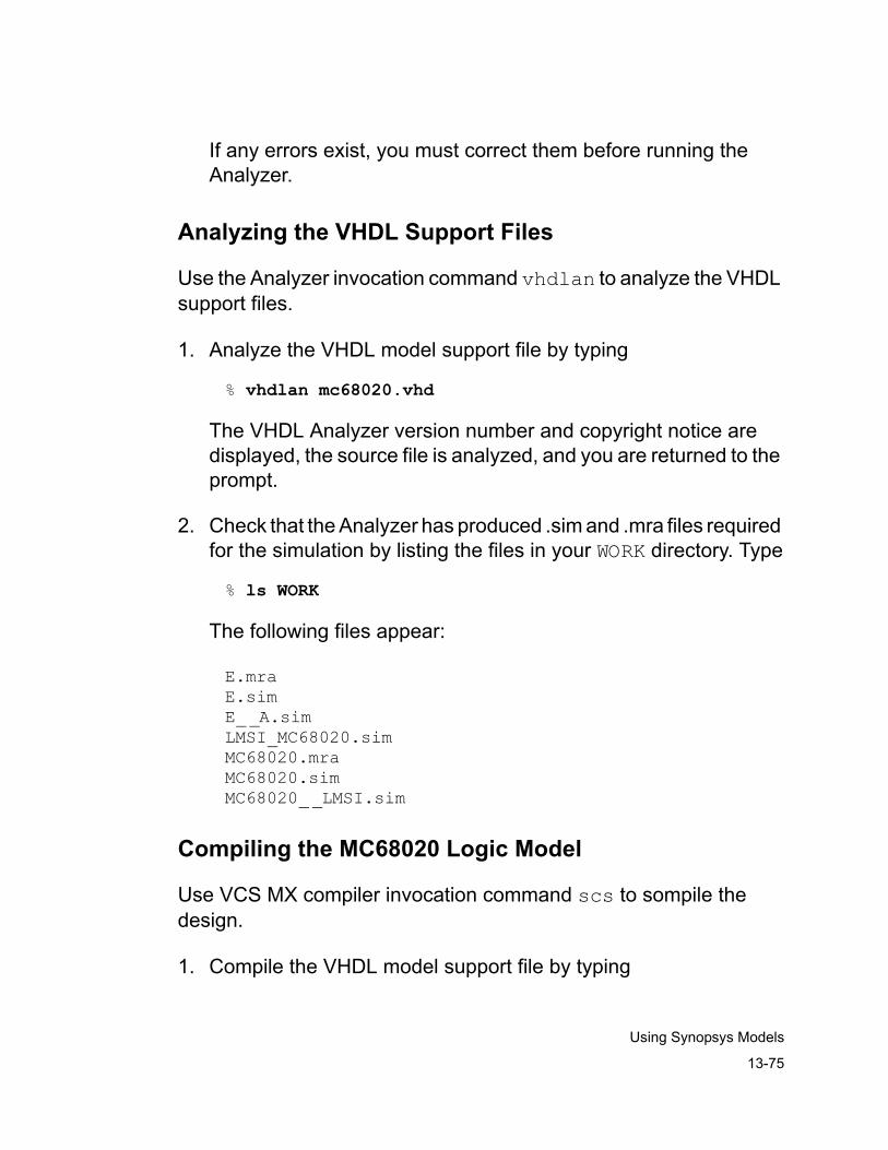
13-75
Using Synopsys Models
If any errors exist, you must correct them before running the Analyzer.
Analyzing the VHDL Support Files
Use the Analyzer invocation command vhdlan to analyze the VHDL support files.
1. Analyze the VHDL model support file by typing
% vhdlan mc68020.vhd
The VHDL Analyzer version number and copyright notice are displayed, the source file is analyzed, and you are returned to the prompt.
2. Check that the Analyzer has produced .sim and .mra files required for the simulation by listing the files in your WORK directory. Type
% ls WORK
The following files appear:
E.mraE.simE__A.simLMSI_MC68020.simMC68020.mraMC68020.simMC68020__LMSI.sim
Compiling the MC68020 Logic Model
Use VCS MX compiler invocation command scs to sompile the design.
1. Compile the VHDL model support file by typing

13-76
Using Synopsys Models
% scs -time NS E
The Compiler version number and copyright notice are displayed, the design is compiled, and you are returned to the prompt.
2. Check that the VCS MX compiler has produced scsim
Simulating the MC68020 Logic Model
You can use the make command to setup this exercise automatically. You then type run at the Simulator prompt to simulate the demonstration. However, to get a good understanding of the exercise, manually execute the steps in this section.
For the first part of the simulation (the reset cycle), the Simulator monitors all CPU signals except the clock. The reset cycle takes 130,250 ns (521 clock cycles.) The initial output (at 0 ns) is the initialization of the model. The output after 130,250 ns, is the deassertion of the reset line on the MC68020. After the reset, this example lists the first few MC68020 cycles.
1. Start up the Simulator by typing
% scsim
The system prints the copyright notice and a message similar to the following:
Warning: scsim,130: From the Logic Modeling Logic Model interface: device_name MC68020: store pins will be played at a maximum device_speed of 7.35 MHz (Message Number: 379)Warning: scsim,130: From the Logic Modeling Logic Model interface: device_name MC68020: Device being modeled with a pattern clock of 14.71 MHz to guarantee 35 ns setup time and 20 ns hold time; actual setup time 35 ns and hold time 20 ns (Message Number: 377)#
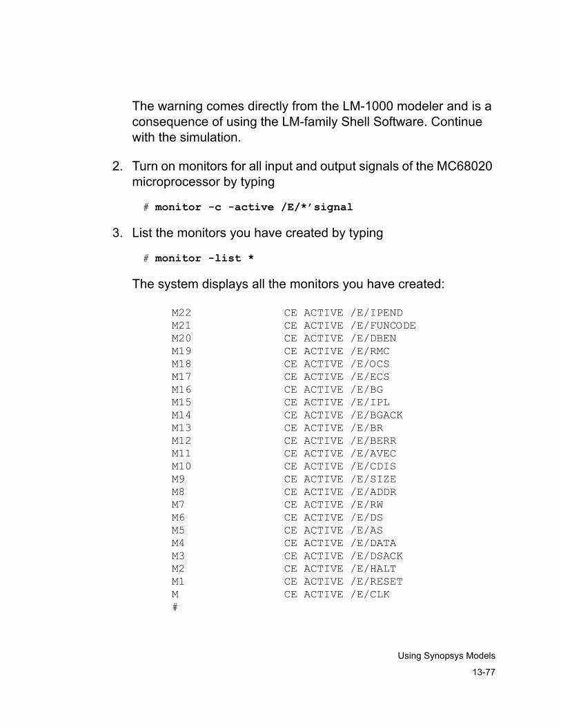
13-77
Using Synopsys Models
The warning comes directly from the LM-1000 modeler and is a consequence of using the LM-family Shell Software. Continue with the simulation.
2. Turn on monitors for all input and output signals of the MC68020 microprocessor by typing
# monitor -c -active /E/*’signal
3. List the monitors you have created by typing
# monitor -list *
The system displays all the monitors you have created:
M22 CE ACTIVE /E/IPENDM21 CE ACTIVE /E/FUNCODEM20 CE ACTIVE /E/DBENM19 CE ACTIVE /E/RMCM18 CE ACTIVE /E/OCSM17 CE ACTIVE /E/ECSM16 CE ACTIVE /E/BGM15 CE ACTIVE /E/IPLM14 CE ACTIVE /E/BGACKM13 CE ACTIVE /E/BRM12 CE ACTIVE /E/BERRM11 CE ACTIVE /E/AVECM10 CE ACTIVE /E/CDISM9 CE ACTIVE /E/SIZEM8 CE ACTIVE /E/ADDRM7 CE ACTIVE /E/RWM6 CE ACTIVE /E/DSM5 CE ACTIVE /E/ASM4 CE ACTIVE /E/DATAM3 CE ACTIVE /E/DSACKM2 CE ACTIVE /E/HALTM1 CE ACTIVE /E/RESETM CE ACTIVE /E/CLK#
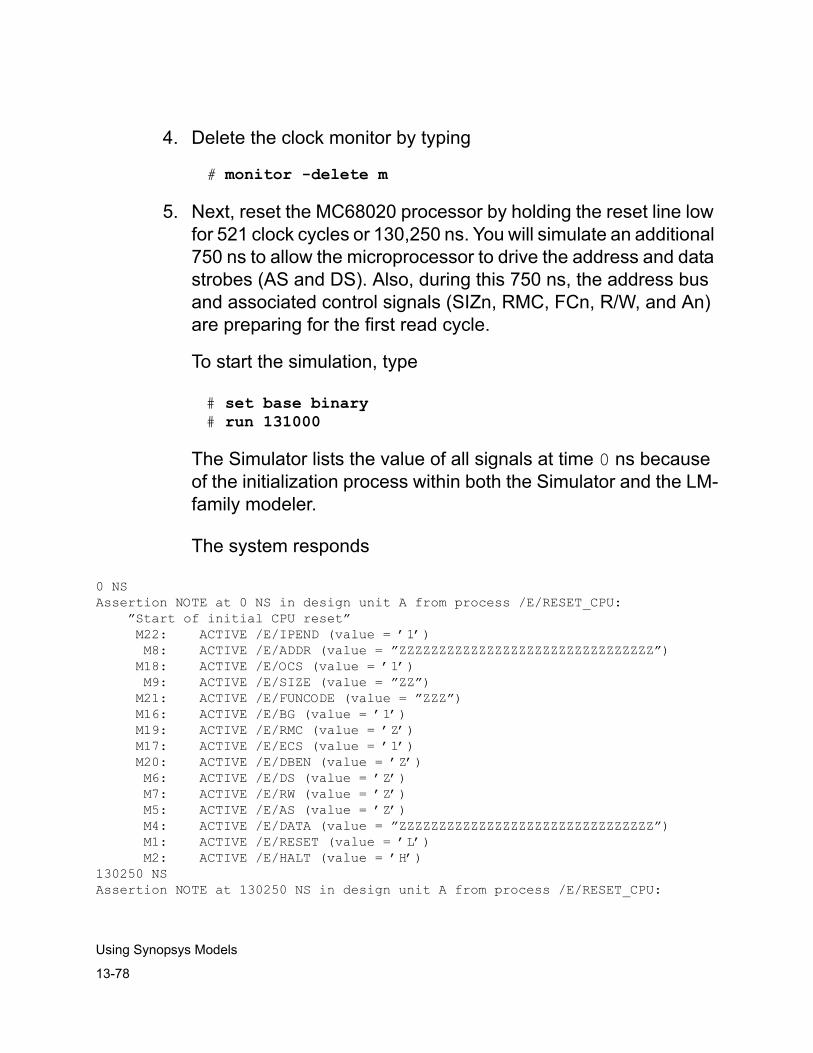
13-78
Using Synopsys Models
4. Delete the clock monitor by typing
# monitor -delete m
5. Next, reset the MC68020 processor by holding the reset line low for 521 clock cycles or 130,250 ns. You will simulate an additional 750 ns to allow the microprocessor to drive the address and data strobes (AS and DS). Also, during this 750 ns, the address bus and associated control signals (SIZn, RMC, FCn, R/W, and An) are preparing for the first read cycle.
To start the simulation, type
# set base binary# run 131000
The Simulator lists the value of all signals at time 0 ns because of the initialization process within both the Simulator and the LM-family modeler.
The system responds
0 NSAssertion NOTE at 0 NS in design unit A from process /E/RESET_CPU: ”Start of initial CPU reset” M22: ACTIVE /E/IPEND (value = ’1’) M8: ACTIVE /E/ADDR (value = ”ZZZZZZZZZZZZZZZZZZZZZZZZZZZZZZZZ”) M18: ACTIVE /E/OCS (value = ’1’) M9: ACTIVE /E/SIZE (value = ”ZZ”) M21: ACTIVE /E/FUNCODE (value = ”ZZZ”) M16: ACTIVE /E/BG (value = ’1’) M19: ACTIVE /E/RMC (value = ’Z’) M17: ACTIVE /E/ECS (value = ’1’) M20: ACTIVE /E/DBEN (value = ’Z’) M6: ACTIVE /E/DS (value = ’Z’) M7: ACTIVE /E/RW (value = ’Z’) M5: ACTIVE /E/AS (value = ’Z’) M4: ACTIVE /E/DATA (value = ”ZZZZZZZZZZZZZZZZZZZZZZZZZZZZZZZZ”) M1: ACTIVE /E/RESET (value = ’L’) M2: ACTIVE /E/HALT (value = ’H’)130250 NSAssertion NOTE at 130250 NS in design unit A from process /E/RESET_CPU:
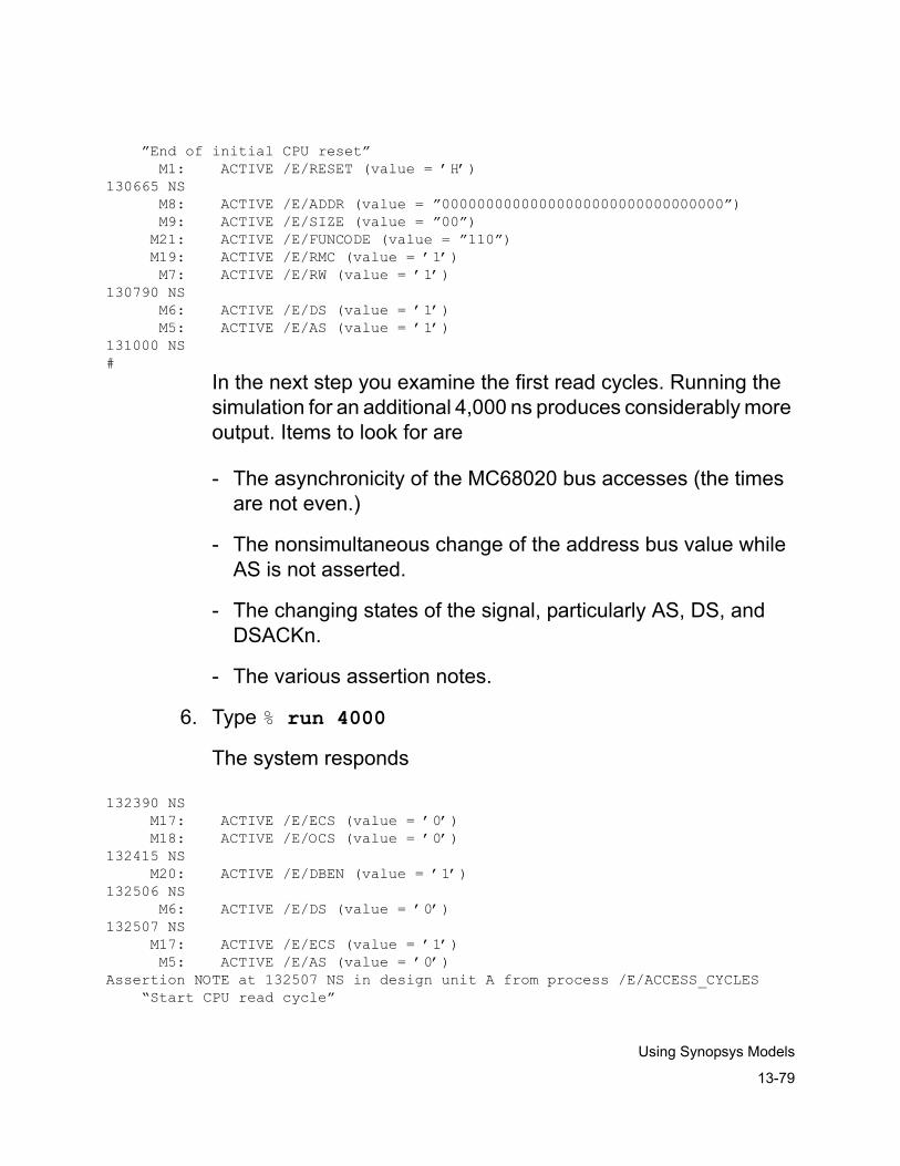
13-79
Using Synopsys Models
”End of initial CPU reset” M1: ACTIVE /E/RESET (value = ’H’)130665 NS M8: ACTIVE /E/ADDR (value = ”00000000000000000000000000000000”) M9: ACTIVE /E/SIZE (value = ”00”) M21: ACTIVE /E/FUNCODE (value = ”110”) M19: ACTIVE /E/RMC (value = ’1’) M7: ACTIVE /E/RW (value = ’1’)130790 NS M6: ACTIVE /E/DS (value = ’1’) M5: ACTIVE /E/AS (value = ’1’)131000 NS#
In the next step you examine the first read cycles. Running the simulation for an additional 4,000 ns produces considerably more output. Items to look for are
- The asynchronicity of the MC68020 bus accesses (the times are not even.)
- The nonsimultaneous change of the address bus value while AS is not asserted.
- The changing states of the signal, particularly AS, DS, and DSACKn.
- The various assertion notes.
6. Type % run 4000
The system responds
132390 NS M17: ACTIVE /E/ECS (value = ’0’) M18: ACTIVE /E/OCS (value = ’0’)132415 NS M20: ACTIVE /E/DBEN (value = ’1’)132506 NS M6: ACTIVE /E/DS (value = ’0’)132507 NS M17: ACTIVE /E/ECS (value = ’1’) M5: ACTIVE /E/AS (value = ’0’)Assertion NOTE at 132507 NS in design unit A from process /E/ACCESS_CYCLES “Start CPU read cycle”
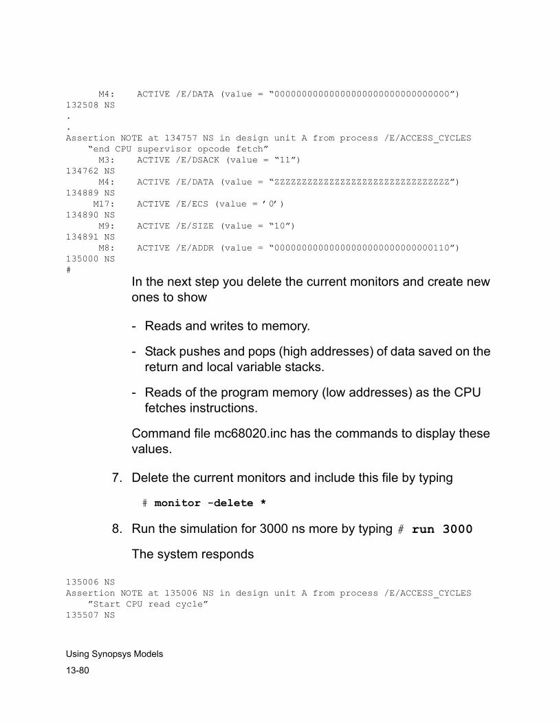
13-80
Using Synopsys Models
M4: ACTIVE /E/DATA (value = “00000000000000000000000000000000”)132508 NS..Assertion NOTE at 134757 NS in design unit A from process /E/ACCESS_CYCLES “end CPU supervisor opcode fetch” M3: ACTIVE /E/DSACK (value = “11”)134762 NS M4: ACTIVE /E/DATA (value = “ZZZZZZZZZZZZZZZZZZZZZZZZZZZZZZZZ”)134889 NS M17: ACTIVE /E/ECS (value = ’0’)134890 NS M9: ACTIVE /E/SIZE (value = “10”)134891 NS M8: ACTIVE /E/ADDR (value = “00000000000000000000000000000110”)135000 NS#
In the next step you delete the current monitors and create new ones to show
- Reads and writes to memory.
- Stack pushes and pops (high addresses) of data saved on the return and local variable stacks.
- Reads of the program memory (low addresses) as the CPU fetches instructions.
Command file mc68020.inc has the commands to display these values.
7. Delete the current monitors and include this file by typing
# monitor -delete *
8. Run the simulation for 3000 ns more by typing # run 3000
The system responds
135006 NSAssertion NOTE at 135006 NS in design unit A from process /E/ACCESS_CYCLES ”Start CPU read cycle”135507 NS
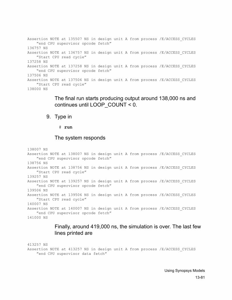
13-81
Using Synopsys Models
Assertion NOTE at 135507 NS in design unit A from process /E/ACCESS_CYCLES ”end CPU supervisor opcode fetch”136757 NSAssertion NOTE at 136757 NS in design unit A from process /E/ACCESS_CYCLES ”Start CPU read cycle”137258 NSAssertion NOTE at 137258 NS in design unit A from process /E/ACCESS_CYCLES “end CPU supervisor opcode fetch”137506 NSAssertion NOTE at 137506 NS in design unit A from process /E/ACCESS_CYCLES ”Start CPU read cycle”138000 NS
The final run starts producing output around 138,000 ns and continues until LOOP_COUNT < 0.
9. Type in
# run
The system responds
138007 NSAssertion NOTE at 138007 NS in design unit A from process /E/ACCESS_CYCLES ”end CPU supervisor opcode fetch”138756 NSAssertion NOTE at 138756 NS in design unit A from process /E/ACCESS_CYCLES ”Start CPU read cycle”139257 NSAssertion NOTE at 139257 NS in design unit A from process /E/ACCESS_CYCLES ”end CPU supervisor opcode fetch”139506 NSAssertion NOTE at 139506 NS in design unit A from process /E/ACCESS_CYCLES ”Start CPU read cycle”140007 NSAssertion NOTE at 140007 NS in design unit A from process /E/ACCESS_CYCLES ”end CPU supervisor opcode fetch”141000 NS
Finally, around 419,000 ns, the simulation is over. The last few lines printed are
413257 NSAssertion NOTE at 413257 NS in design unit A from process /E/ACCESS_CYCLES ”end CPU supervisor data fetch”
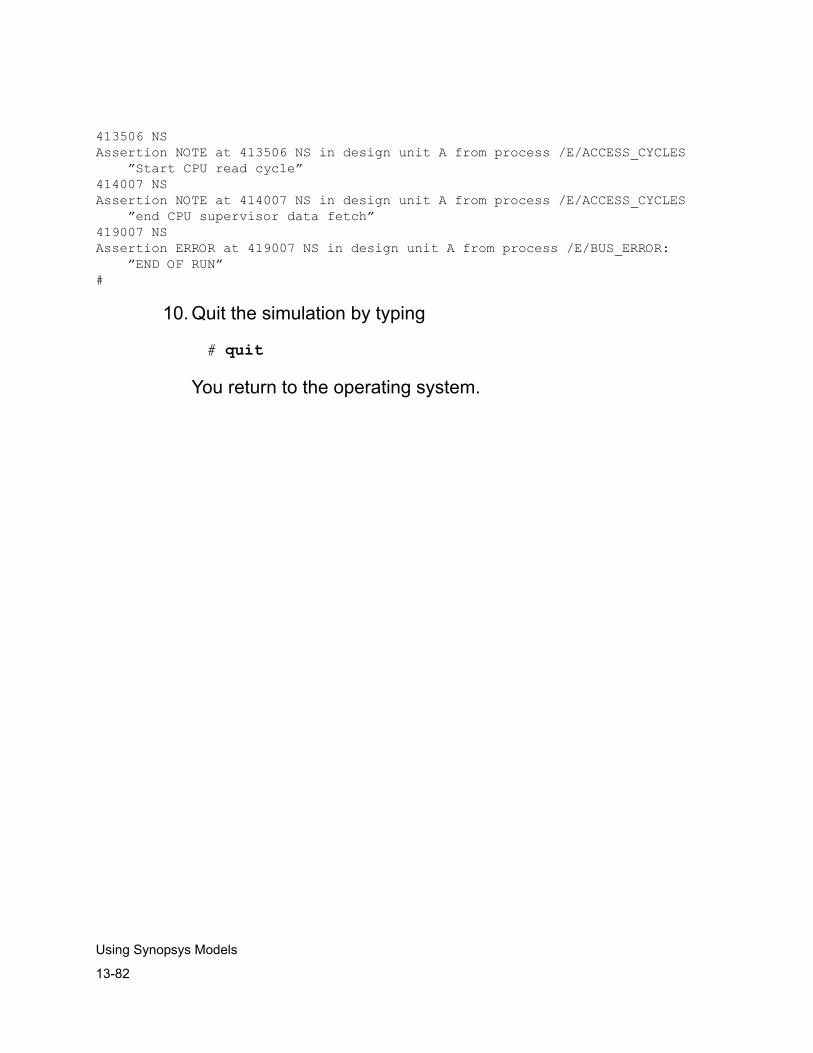
13-82
Using Synopsys Models
413506 NSAssertion NOTE at 413506 NS in design unit A from process /E/ACCESS_CYCLES ”Start CPU read cycle”414007 NSAssertion NOTE at 414007 NS in design unit A from process /E/ACCESS_CYCLES ”end CPU supervisor data fetch”419007 NSAssertion ERROR at 419007 NS in design unit A from process /E/BUS_ERROR: ”END OF RUN”#
10. Quit the simulation by typing
# quit
You return to the operating system.
A-1
Backannotating with SDF Files
ABackannotating with SDF Files A
You can backannotate timing information from files in Standard Delay File (SDF) format into your design before or during simulation. SDF format is commonly used to communicate timing information among different simulators, synthesis tools, and layout tools.
You can use SDF files obtained from your ASIC vendor, generate them using Synopsys Design Compiler or third-party tools, or write them yourself. See the OVI Standard Delay File (SDF) Format Specification published by Open Verilog International for instructions on writing an SDF file.
For information about using SDF version 3.0, see “SDF Version 3.0 in Appendix A”.

A-2
Backannotating with SDF Files
To backannotate your design with SDF timing data, you need to understand the following topics:
• Specifying the SDF files
• Examining SDF header information
• Matching SDF timing parameters to generic parameters
• Understanding device constructs
• Annotating single bits
• Backannotation restrictions
• Ignored SDF constructs
• Backannotating structural library cells
Specifying the SDF Files
There are two ways to indicate the SDF files for backannotation:
• With the scsim command
• With the simulator include command. This applies only to RTL or non-VITAL libraries.
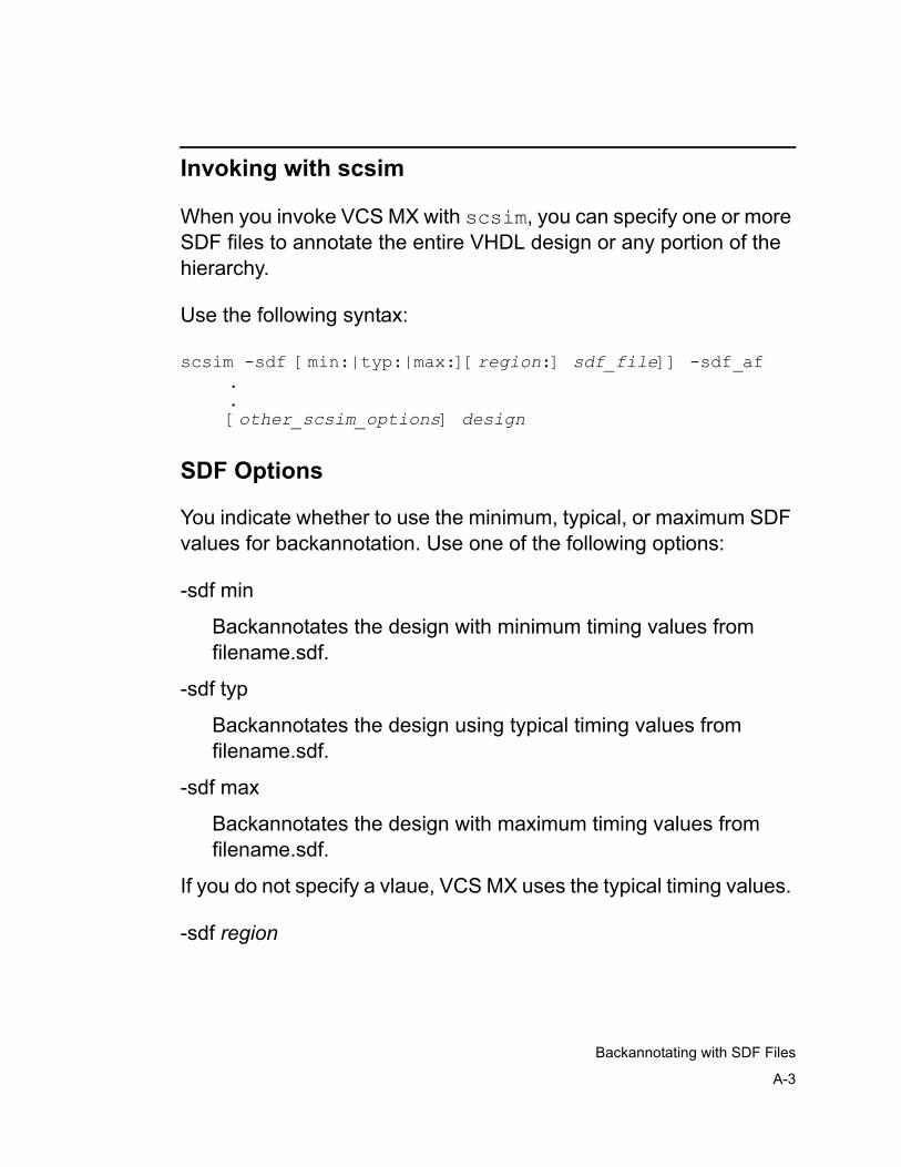
A-3
Backannotating with SDF Files
Invoking with scsim
When you invoke VCS MX with scsim, you can specify one or more SDF files to annotate the entire VHDL design or any portion of the hierarchy.
Use the following syntax:
scsim -sdf [min:|typ:|max:][region:] sdf_file]] -sdf_af..[other_scsim_options] design
SDF Options
You indicate whether to use the minimum, typical, or maximum SDF values for backannotation. Use one of the following options:
-sdf min
Backannotates the design with minimum timing values from filename.sdf.
-sdf typ
Backannotates the design using typical timing values from filename.sdf.
-sdf max
Backannotates the design with maximum timing values from filename.sdf.
If you do not specify a vlaue, VCS MX uses the typical timing values.
-sdf region

A-4
Backannotating with SDF Files
Backannotates the portion of the design below region, using timing values from sdf_file.sdf.
-sdf_af
Creates an assign file that contains generics and their values from filename.sdf. The assign file is called filename.inc. This file is useful only for debugging the SDF file.
Examples
The following example uses timing data from two different SDF files to annotate two different portions of a design:
% scsim -sdf /E/UUT/DESIGN1:myfile1.sdf \ -sdf max:/E/UUT/DESIGN2:myfile2.sdf
The above command
• Backannotates the VHDL design cfg, starting from /E/UUT/DESIGN1, with typical timing values (the default) from the SDF file myfile1.sdf.
• Backannotates the VHDL design cfg starting from /E/UUT/DESIGN2 with the maximum timing values from the SDF file myfile2.sdf.
The following example shows how to use two SDF files to backannotate the same portion of a VHDL design:
% scsim -sdf min:/E/UUT/DESIGN:myfile1.sdf -sdf myfile2.sdf
The above command backannotates the VHDL design cfg starting from /E/UUT/DESIGN using the minimum timing values from both myfile1.sdf and myfile2.sdf.
A-5
Backannotating with SDF Files
Invoking with the Simulator include Command
After you start VCS MX, you can specify the SDF file for RTL or non-VITAL libraries with the simulator include command, as follows:
include [sdf_value_option] [other_sdf_options]\ -sdf sdf_filename
SDF Options
sdf_value_option indicates whether to use the minimum, typical, or maximum SDF values for backannotation. Use one of the following options:
-sdf_min
Backannotates the design with minimum timing values from filename.sdf.
-sdf_typ
Backannotates the design using typical timing values from filename.sdf.
-sdf_max
Backannotates the design with maximum timing values from filename.sdf.
If you do not specify sdf_value_option, VCS MX uses the typical timing values. If you use the -sdf_top, -sdf_min, -sdf_max, or -sdf_typ options, you must place them before the -sdf filename to apply them to filename.
other_sdf_options is one of the following:
-sdf_top declarative_region
A-6
Backannotating with SDF Files
Backannotates the portion of the design below declarative_region, using timing values from filename.sdf.
-sdf_af
Creates an assign file that contains generics and their values from filename.sdf. The assign file is called filename.inc. This file is useful only for debugging the SDF file.
You must specify precisely where you want to annotate (sdf_top), how you want to annotate (min, typ, or max), and the filename. If you want to use more than one SDF file, you can repeat the include command, once for each additional SDF file.
For example, the commands
# include -sdf_top /e/b1 -sdf_min -sdf timing1.sdf# include -sdf_top /e/b2 -sdf_typ -sdf timing2.sdf
backannotate the design with the minimum timing values from the timing1.sdf file with the typical values from timing2.sdf.
The timing information in the SDF files can cover the whole VHDL design or any portion of the hierarchy. If more than one SDF file annotates the same instance, the last SDF file read overwrites all previous ones.
To use the wildcard (*) in SDF files, set the SDFWILDCARD setup variable to true. The default is false. To turn on wildcard capability, put the following entry in your synopsys_sim.setup file:
SDFWILDCARD = true
A-7
Backannotating with SDF Files
Note:Set this flag to TRUE only to use an SDF file that contains wildcard constructs. Setting this flag to TRUE can slow down elaboration and increase the amount of memory VCS MX uses.
Examining SDF Header Information
The header file contains information about conditions under which the SDF file was created. For example, the name of the program that generated the file, date of generation, ambient temperature, and so on.
If you want to examine the header information from the SDF file, use the following procedure:
1. Include the package header file, sdf_header.vhd, in your testbench VHDL file. To do this, add the following line at the beginning of your testbench file, before the first entity:
use synopsys.sdf_header.all;
The header file is located in the directory $VCS_HOME/packages/synopsys/src. This file is automatically updated when you read in the SDF file.
2. Invoke VCS MX (scsim) on your design.
3. Use the simulator ls command at the top level of your design.
# ls -v sdf_header
VCS MX displays the SDF header information.
A-8
Backannotating with SDF Files
Matching SDF Timing Parameters to VHDL Generics
During backannotation, VCS MX reads the values for SDF timing parameters from the SDF file, then assigns the values to the appropriate VHDL generic parameters in your design. This applies only for non-VITAL libraries.
Understanding Naming Conventions
The simulator matches the VHDL generic parameter names with SDF timing parameter names according to the convention shown in Table A-1. The table describes the default naming convention for all the timing parameters.
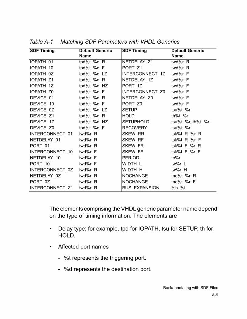
A-9
Backannotating with SDF Files
Table A-1 Matching SDF Parameters with VHDL Generics
The elements comprising the VHDL generic parameter name depend on the type of timing information. The elements are
• Delay type; for example, tpd for IOPATH, tsu for SETUP, th for HOLD.
• Affected port names
- %t represents the triggering port.
- %d represents the destination port.
SDF Timing Default Generic Name
SDF Timing Default Generic Name
IOPATH_01 tpd%t_%d_R NETDELAY_Z1 twd%r_RIOPATH_10 tpd%t_%d_F PORT_Z1 twd%r_RIOPATH_0Z tpd%t_%d_LZ INTERCONNECT_1Z twd%r_FIOPATH_Z1 tpd%t_%d_R NETDELAY_1Z twd%r_FIOPATH_1Z tpd%t_%d_HZ PORT_1Z twd%r_FIOPATH_Z0 tpd%t_%d_F INTERCONNECT_Z0 twd%r_FDEVICE_01 tpd%t_%d_R NETDELAY_Z0 twd%r_FDEVICE_10 tpd%t_%d_F PORT_Z0 twd%r_FDEVICE_0Z tpd%t_%d_LZ SETUP tsu%t_%rDEVICE_Z1 tpd%t_%d_R HOLD th%t_%rDEVICE_1Z tpd%t_%d_HZ SETUPHOLD tsu%t_%r, th%t_%rDEVICE_Z0 tpd%t_%d_F RECOVERY tsu%t_%rINTERCONNECT_01 twd%r_R SKEW_RR tsk%t_R_%r_RNETDELAY_01 twd%r_R SKEW_RF tsk%t_R_%r_FPORT_01 twd%r_R SKEW_FR tsk%t_F_%r_RINTERCONNECT_10 twd%r_F SKEW_FF tsk%t_F_%r_FNETDELAY_10 twd%r_F PERIOD tc%rPORT_10 twd%r_F WIDTH_L tw%r_LINTERCONNECT_0Z twd%r_R WIDTH_H tw%r_HNETDELAY_0Z twd%r_R NOCHANGE tnc%t_%r_RPORT_0Z twd%r_R NOCHANGE tnc%t_%r_FINTERCONNECT_Z1 twd%r_R BUS_EXPANSION %b_%i
A-10
Backannotating with SDF Files
- %r represents the reference port.
- %b represents the bus name.
- %i represents the index of the bus.
• %T represents either the null string or the string ”out”. This element is used in the generic names associated with interconnect delays.
The interconnect delay between an output (or bidirectional) port of an instance and an output (or bidirectional) port of a design requires special handling by the backannotation mechanism. For such delays, %T=”out”; for all other interconnect delays, %T is the null string.
Note:For interconnect delays with %T=”out”, the cell model must include an output wire buffer at the instance port, to serve as a delay site.
Changing the Naming Convention
You can change the naming convention of one or more of the SDF generics, or you can add new ones in a text file called sdf_naming_file.s. You identify the path to the sdf_naming_file.s file with the following entry in the synopsys_sim.setup file:
SDFNAMINGFILE = path/sdf_naming.s
path is the full pathname to the naming file.

A-11
Backannotating with SDF Files
You can create another naming convention for any or all SDF timing parameters listed in Table A-1. For example, your naming file may contain the following lines:
IOPATH_01 = %t_mytpd%r_01INTERCONNECT_Z1 = my_interconnect_Z1
Understanding the DEVICE Construct
The DEVICE construct specifies the intrinsic delay of a cell or gate. When VCS MX reads a DEVICE construct, it backannotates the pin-to-pin delay generics throughout the cell. How the simulator handles the DEVICE construct depends on whether or not the construct includes an output port name.
• If DEVICE includes an output port name (for example, (DEVICE Out1 (1:2:3)), VCS MX assigns the timing value only to those pin-to-pin delay generics in the cell with that output port name as their destination. For example, during backannotation of the device in Figure A-1, if the DEVICE construct is
DEVICE Out1 (1:2:3) (1:2:3)
VCS MX assigns the timing value only to the following generics:
tpdIn1_Out1_R, tpdIn1_Out1_F, tpdIn2_Out1_R, and tpdIn2_Out1_F
It ignores the generics such as tpdIn1_Out2_R, tpdIn1_Out2_F, tpdIn2_Out2_R, and tpdIn2_Out2_F.
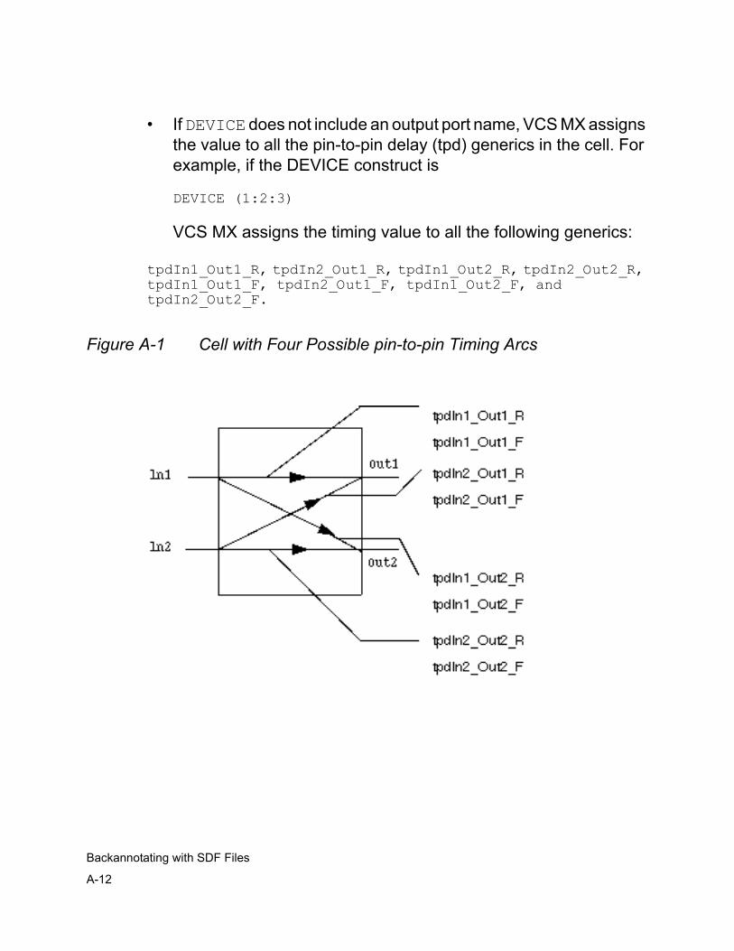
A-12
Backannotating with SDF Files
• If DEVICE does not include an output port name, VCS MX assigns the value to all the pin-to-pin delay (tpd) generics in the cell. For example, if the DEVICE construct is
DEVICE (1:2:3)
VCS MX assigns the timing value to all the following generics:
tpdIn1_Out1_R, tpdIn2_Out1_R, tpdIn1_Out2_R, tpdIn2_Out2_R, tpdIn1_Out1_F, tpdIn2_Out1_F, tpdIn1_Out2_F, and tpdIn2_Out2_F.
Figure A-1 Cell with Four Possible pin-to-pin Timing Arcs
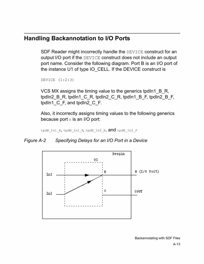
A-13
Backannotating with SDF Files
Handling Backannotation to I/O Ports
SDF Reader might incorrectly handle the DEVICE construct for an output I/O port if the DEVICE construct does not include an output port name. Consider the following diagram. Port B is an I/O port of the instance U1 of type IO_CELL. If the DEVICE construct is
DEVICE (1:2:3)
VCS MX assigns the timing value to the generics tpdIn1_B_R, tpdIn2_B_R, tpdIn1_C_R, tpdIn2_C_R, tpdIn1_B_F, tpdIn2_B_F, tpdIn1_C_F, and tpdIn2_C_F.
Also, it incorrectly assigns timing values to the following generics because port B is an I/O port:
tpdB_In1_R, tpdB_In1_F, tpdB_In2_R, and tpdB_In2_F
Figure A-2 Specifying Delays for an I/O Port in a Device
A-14
Backannotating with SDF Files
To handle I/O ports, use the INTERCONNECT construct instead of the DEVICE construct.
Using the INTERCONNECT Construct
The INTERCONNECT construct represents the actual or estimated delay in the wire between devices.
The following SDF specifies the loading for Figure A-2:
(INSTANCE CELLTYPE)(DELAY(ABSOLUTE(INTERCONNECT U1/B A (2:3:4))))
In the above statements, the interconnect must be reflected at the input of the next stage (which is actually the load or tester in this case). Since this is not available for simulation purposes, this interconnect is added to the output of the previous stage.
But the intent of the SDF entry was to backannotate to all generics that use B as an output port. In this case, the following SDF entry yields correct backannotation:
(DEVICE B (1:2:3))
Multiple Backannotations to Same Delay Site
VCS MX backannotates source to load delays onto the delay site associated with the load port. Therefore, there are multiple delay entries, from different source ports to the same load port. In such cases, you can specify the delay value that you want to backannotate.
A-15
Backannotating with SDF Files
The SDFPOLICY variable allows you to select the backannotation delay value. You can set this variable to MIN, MAX, or MINOMAX. The default value is MAX for backwards compatibility. If you specify a value other than MIN, MAX, or MINOMAX, VCS MX issues a warning and uses MAX as the default value.
For example, consider the generics tpdA_Y_R and tpdA_Y_F and the following SDF file:
(IOPATH A Y (1:2:3) (3:4:5))(IOPATH A Y (7:8:9) (1:2:3)(IOPATH A Y (3:4:5) (7:8:9))
Assume you run a typical simulation run. If the synopsys_sim.setup file includes the following entry:
SDFPOLICY = MIN
the backannotation retains the minimum values on the corresponding generics (seen by the ls -v command):
tpdA_Y_R 2 nstpdA_Y_F 2 ns
If the synopsys setup file had no SDFPOLICY entry or the entry was as follows:
SDFPOLICY = MAX
the backannotation retains the maximum values on the corresponding generics (seen by the ls -v command):
tpdA_Y_R 8 nstpdA_Y_F 8 ns
A-16
Backannotating with SDF Files
If the synopsys setup file includes the following entry:
SDFPOLICY = MINOMAX
the minimum of all possible values are selected during a minimum simulation run, and the maximum of all possible values are selected for typical and maximum simulation runs. Therefore, during a minimum simulation run (specified on the simulator command line via the -sdf_min flag), the backannotation retains the following values on the corresponding generics:
tpdA_Y_R 1 nstpdA_Y_F 1 ns
during a typical simulation run, the following values are retained:
tpdA_Y_R 8 nstpdA_Y_F 8 ns
Whereas in a maximum simulation run, the following values are retained:
tpdA_Y_R 9 nstpdA_Y_F 9 ns
If the synopsys setup file had an illegal value specified such as the following:
SDFPOLICY = illegal
VCS MX issues the following warning message:
Warning: scsim,180:Bad value specified for “SDFPOLICY”, using default: MAX.
A-17
Backannotating with SDF Files
and the backannotation retains the following maximum values on the corresponding generics (seen by the ls -v command) during a typical simulation run:
tpdA_Y_R 8 nstpdA_Y_F 8 ns
Annotating Single Bits
You can backannotate a single bit in any SDF construct where an SDF BIT_SPEC (bit specification) is valid. For example:
(IOPATH i[1] b[2] (1:2:3) (4:5:6))
However, you cannot annotate a range of bits. For example, VCS MX ignores the following construct:
(IOPATH I[1:2] B[2:3] (1:2:3:) (4:5:6))
The generic naming convention for a single bit is %b_%i, where
• %b is the name of the bus.
• %i is the element index in the bus.
For example, the SDF construct
(IOPATH I[1] B[2] (1:2:3) (4:5:6))
A-18
Backannotating with SDF Files
causes VCS MX to expect the following default generic parameters in the VHDL file:
• tpdI_1_B_2_R
• tpdI_1_B_2_F
If you want to change the default naming convention for single-bit backannotation, place the BUS_EXPANSION variable in your SDF naming file. Set the variable equal to your new naming convention. For example,
BUS_EXPANSION = %i_%b.
causes VCS MX to look for the generics tpd1_I_2_B_R and tpd1_I_2_B_F in the previous example.
Back-Annotation Restrictions
Keep in mind these important points when backannotating with SDF files:
• If there is one triplet in an IOPATH construct, VCS MX backannotates both the rise time and fall time for the path. The following example annotates both the rise and fall time of the path:
IOPATH CLK Q (1.109:1.445:2.335)
• If you want to only annotate the rise or fall time, you must use a null transition (empty set of parentheses) for the delay you do not want to annotate. The following example annotates only the rise time:
IOPATH CLK Q (1.204:1.535:2.478) ()
A-19
Backannotating with SDF Files
• If you use conditional statements in the SDF file, you must make sure that the conditional expression exactly matches the condition in the VHDL model, except for white spaces such as tabs or blanks.
For example, the following SDF statement:
COND ( B == 1’b0 ) (IOPATH A Q ...
does not match the condition in the VHDL model
attribute SDT_CONDITION of tpdA_Q_R: constant is“ B == 1’b0 , B == 1’b1”;
To make these two statements match, the extra parenthesis are removed from the SDF statement as follows:
COND B == 1’b0 (IOPATH A Q ...
Ignored SDF Constructs
VCS MX supports only those SDF constructs that are meaningful during VHDL simulation. It ignores the following SDF timing constructs:
PATHPULSE
Pulse rejection limit and the X limit.
GLOBALPATHPULSE
Pulse rejection limit and the X limit measured in percentage of cell path delay.
A-20
Backannotating with SDF Files
PATHCONSTRAINT
Time constraint for circuit paths in timing analysis applications.
SUM
Total of the individual delays associated with start-end port pair and its limit.
DIFF
Maximum difference in delay between two paths.
SKEWCONSTRAINT
Maximum skew delay associated with ports.
Edge Specifier
Positive edge and negative edge, except for the constructs WIDTH and NOCHANGE.
Back-Annotating Structural Library Cells
You can change the value of behavioral cell generic parameters after elaboration, because the value of the generic is read each time the cell is active. Structural cells, however, use the value of the cell level generic in the generic map of lower level structural instances.
VCS MX does not automatically propagate changes to generic values to the places where that generic is used. Therefore, when creating a structural library cell, you must identify the lower-level generic that must also be updated. You do this by assigning the PROPAGATE_VALUE attribute in the architecture declaration of the structural cell.
attribute PROPAGATE_VALUE of generic: constant is ”generic_name_list”;
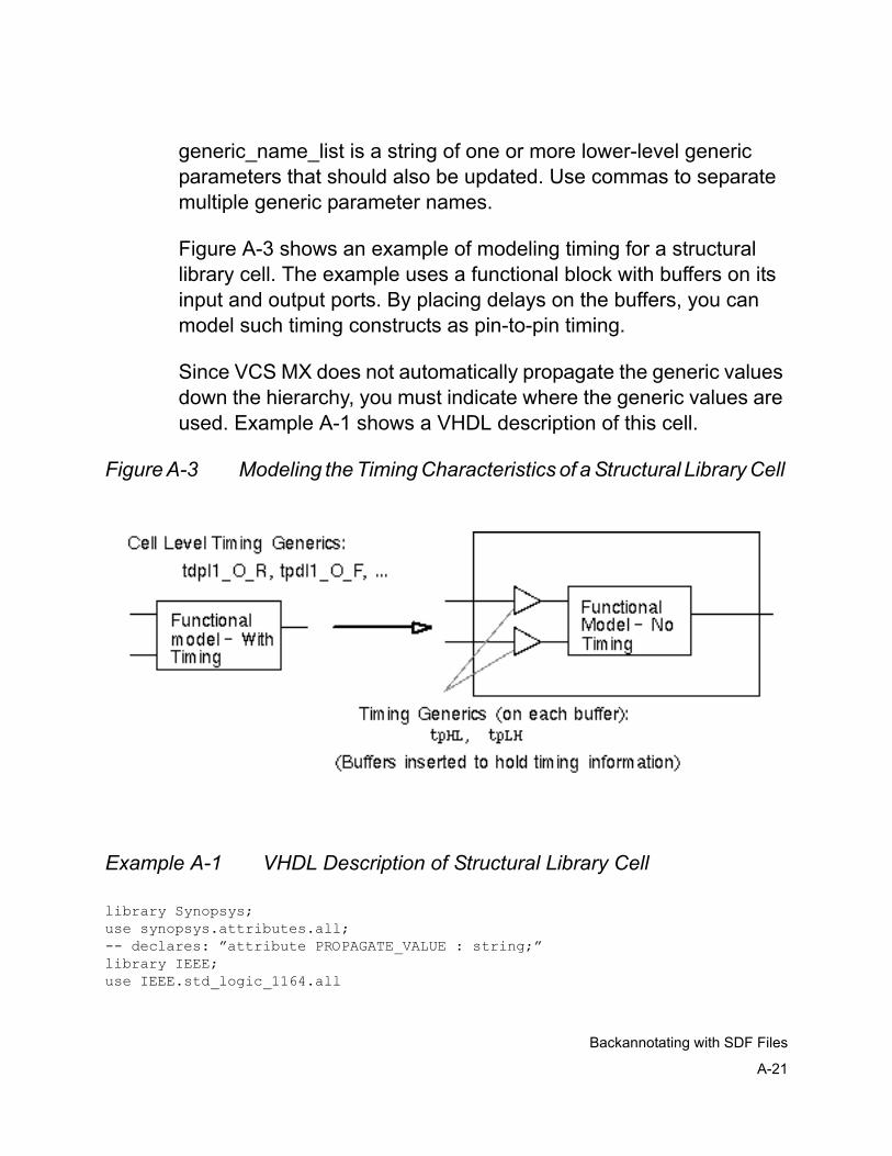
A-21
Backannotating with SDF Files
generic_name_list is a string of one or more lower-level generic parameters that should also be updated. Use commas to separate multiple generic parameter names.
Figure A-3 shows an example of modeling timing for a structural library cell. The example uses a functional block with buffers on its input and output ports. By placing delays on the buffers, you can model such timing constructs as pin-to-pin timing.
Since VCS MX does not automatically propagate the generic values down the hierarchy, you must indicate where the generic values are used. Example A-1 shows a VHDL description of this cell.
Figure A-3 Modeling the Timing Characteristics of a Structural Library Cell
Example A-1 VHDL Description of Structural Library Cell
library Synopsys;use synopsys.attributes.all; -- declares: ”attribute PROPAGATE_VALUE : string;”library IEEE;use IEEE.std_logic_1164.all
A-22
Backannotating with SDF Files
use IEEE.std_logic_components.all;
entity E isgeneric(tpdA_Z_R, tpdA_Z_F: time);port (A: in std_logic; Z: out std_logic);
end;
architecture A of E isattribute PROPAGATE_VALUE of tpdA_Z_R: constant is ”U1/tpHL”;attribute PROPAGATE_VALUE of tpdA_Z_F: constant is ”U1/tpHL”;attribute PROPAGATE_VALUE of tpdA_Z_F:
constant is ”U2/tpHL, U3/tpHL”;...
signal S: std_logic;begin
U1: BUFGATE -- Buffer to hold the timinggeneric map(tpLH => tpdA_Z_R, tpHL => tpdA_Z_F)port map(A, S);Z <= S;-- Functional block
.
.
.end A;
You can map several SDF timing values to either the same cell-level generics or the same lower-level generics. VCS MX applies the largest timing value to the generic.
SDF Back-Annotation for Gate-Level Timing Simulation
VHDL VITAL gate level simulation performance is very slow compared to Verilog gate level simulation. Synopsys recommends using the VCS MX flow with VHDL testbench environment and Verilog netlist.
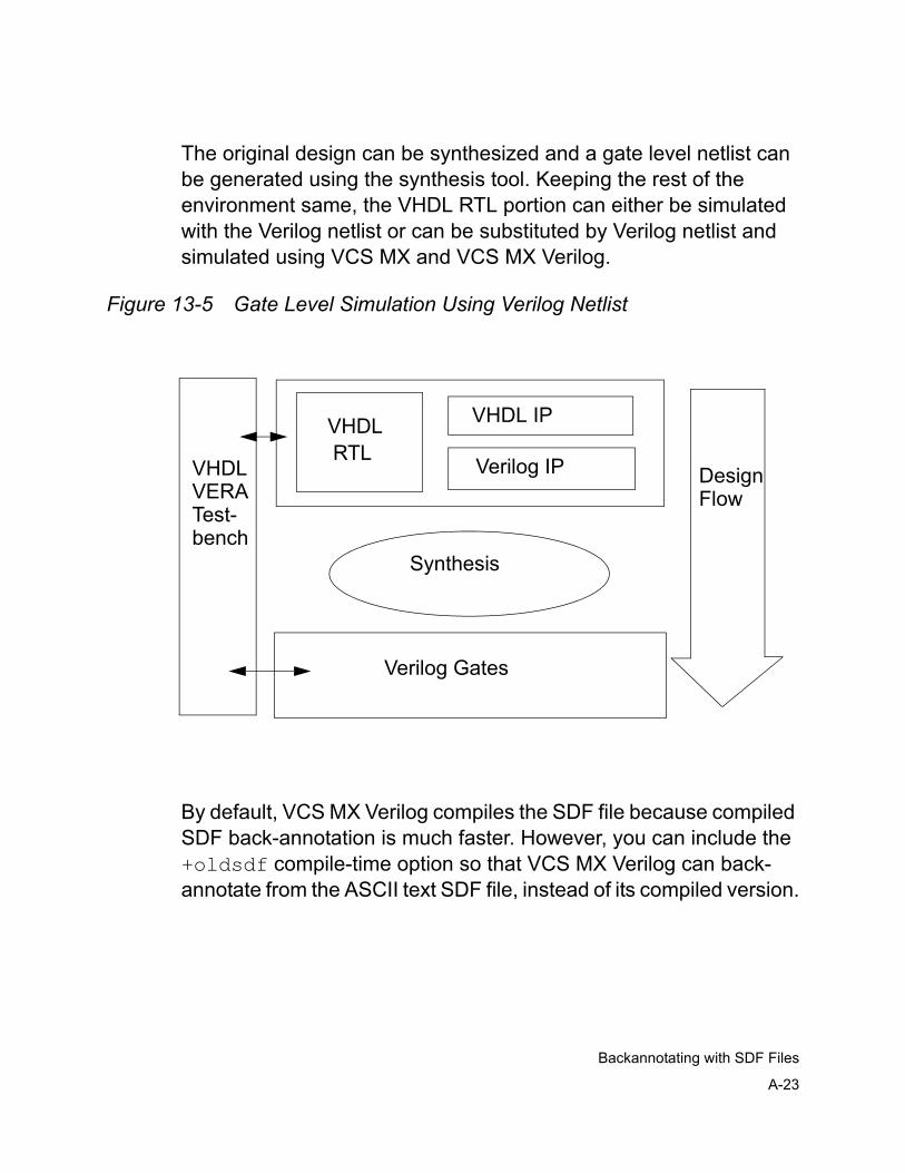
A-23
Backannotating with SDF Files
The original design can be synthesized and a gate level netlist can be generated using the synthesis tool. Keeping the rest of the environment same, the VHDL RTL portion can either be simulated with the Verilog netlist or can be substituted by Verilog netlist and simulated using VCS MX and VCS MX Verilog.
Figure 13-5 Gate Level Simulation Using Verilog Netlist
By default, VCS MX Verilog compiles the SDF file because compiled SDF back-annotation is much faster. However, you can include the +oldsdf compile-time option so that VCS MX Verilog can back-annotate from the ASCII text SDF file, instead of its compiled version.
DesignFlow
VHDLRTL
VHDL IP
Verilog IP
Synthesis
Verilog Gates
VHDLVERATest-bench
A-24
Backannotating with SDF Files
You can not back-annotate delay values through SDF back-annotation on the entire mixed language design simultaneously but you can always back-annotate delay values from an SDF file to the Verilog netlist. SDF file must have the same design name as the module name of the netlist which is instantiated in VHDL.
For simple Verilog netlist timing simulation using compiled SDF back-annotation, you must follow these steps:
1. Specify the $sdf_annotate system task in the Verilog netlist (top level module) with the netlist module name and SDF file. For example,
$sdf_annotate (“SDF_File”, Module_Name);
Specifying Module name is optional. By default, since the task is in the netlist module, the SDF back-annotation will be performed on the same netlist module.
If you specify a module_instance argument in the $sdf_annotate system task, you cannot enter an absolute hierarchical name for the module instance. You can only enter a relative hierarchical module name. An absolute hierarchical name begins with the name of a top-level module in the Verilog design that you instantiate in the VHDL design. Entering this hierarchical name is not absolute because the root of absolute hierarchical names in VCS MX flow is up in the VHDL part of the design. A relative hierarchical name begins with a module instance name of a module instance that is instantiated in the module definition that contains the $sdf_annotate system task.
For example, if TOP_GATE (netlist, Verilog) is instantiated in TB_TOP_GATE (VHDL) as VLOG_GATES (instance name, VHDL), the correct specification of $sdf_annotate task in Verilog netlist (TOP_GATE) is
A-25
Backannotating with SDF Files
$sdf_annotate(“SDF_FILE”, TOP_GATE);
and not
$sdf_annotate(“SDF_FILE”, VLOG_GATES);
Note :
a. You can not specify $sdf_annotate in a separate Verilog module.
b. Although specifying module instance name instead of module name is supported, because of complications in specifying the correct hierarchical path for the netlist instance, it is recommended not to use this method but instead use the method explained above.
2. Follow the steps mentioned in VCS MX flow.
- Instantiate the Verilog netlist module in VHDL design using component declaration and instantiation.
- Analyze Verilog netlist along with library modules.
% vlogan netlist.v \-v /design/syn/lib_file \-y /design/syn/lib_dir1 +libext+.v \+notimingchecks
You must specify all the required source files (with the netlist), library files, and directories needed for Verilog portion. All the rules mentioned earlier regarding library files and directories apply.
- Analyze VHDL design units including one which instantiates Verilog netlist.
A-26
Backannotating with SDF Files
- Elaborate VHDL design units and compile Verilog netlist using correct options for scs. For example,
% scs lib.cfg_tb_gate -verilogcomp “+rad+1”
- Simulate the entire design using scsim with correct usage of run-time options.
% scsim -verilogrun “+notimingchecks”

B-1
Using VITAL Models and Netlists
BUsing VITAL Models and Netlists B
You use VHDL Analyzer and VCS MX to validate and optimize a VHDL initiative toward ASIC libraries (VITAL) model and to simulate a VITAL-based netlist. Typically, the optimization of the VITAL model is done by library developers, and simulation of the VITAL-based netlist is done by designers.
The library developer uses a single ASIC cell from the system, verifies its correctness, and optimizes that single cell. The designer simulates large numbers of cells, organized in a netlist, by applying test vectors and timing information.
This chapter describes how the library developer can validate and optimize a VITAL model and how the designer can simulate a VITAL netlist.
B-2
Using VITAL Models and Netlists
Validating and Optimizing a VITAL Model
The library developer performs the following tasks:
• Validates the model for VITAL conformance
• Verifies the model for functionality
• Optimizes the model for performance and capacity
• Re-verifies the model for functionality
Validating the Model for VITAL Conformance
Library developers can validate the conformance of the VHDL design units to VITAL 95 IEEE specifications, according to level 0 or level 1 as specified in the model, by using vhdlan.
vhdlan checks the VITAL design units for conformance when you set the VITAL attribute on the entity (VITAL_Level0) and architecture (VITAL_Level1) to TRUE. vhdlan does not check the design unit for VITAL conformance if the attribute is set to FALSE.
Verifying the Model for Functionality
Library developers then verify the model’s functions by using scsim. The functional verification includes checking the following:
• Timing values for the cell, including hazard detection
• Correct operation of the timing constraints and violation detection
• Other behavioral aspects of the cell according to specifications
B-3
Using VITAL Models and Netlists
Optimizing the Model for Performance and Capacity
Library developers compile the VHDL design units to optimize the model for simulation by using vhdlan. vhdlan checks the design unit for VITAL conformance before performing any optimization.
To optimize the design units, perform the following steps:
1. Set the VITAL attribute on the entity (VITAL_Level0) and on the architecture (VITAL_Level1) to TRUE.
When you optimize architectures that have the VITAL_Level1 attribute set to TRUE, visibility into the cell is lost and the cell is marked as PRIVATE. Ports and generics remain visible.
2. Use either the OPTIMIZE variable in the setup file or -optimize option to the vhdlan command.
The command line option overrides the setting in the synopsys_sim.setup file.
a. Set the OPTIMIZE variable in the setup fileTable B-1 lists the legal values of the variable, the design unit type, and the results of each setting.
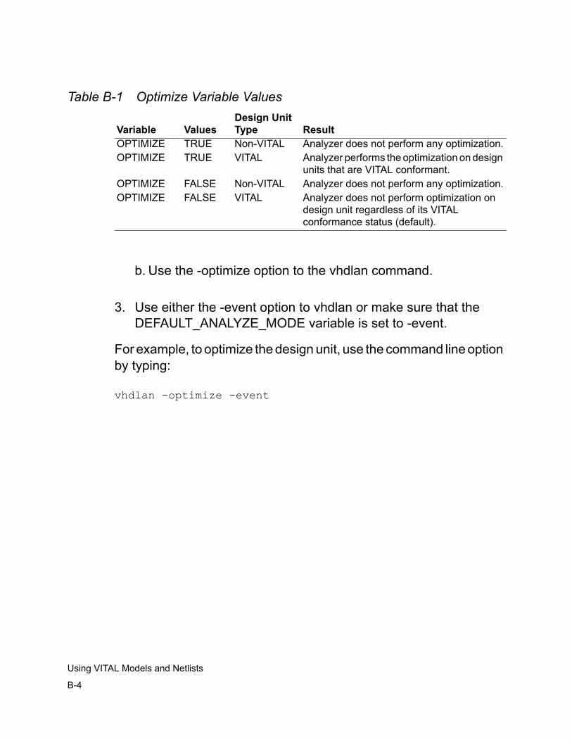
B-4
Using VITAL Models and Netlists
Table B-1 Optimize Variable Values
b. Use the -optimize option to the vhdlan command.
3. Use either the -event option to vhdlan or make sure that the DEFAULT_ANALYZE_MODE variable is set to -event.
For example, to optimize the design unit, use the command line option by typing:
vhdlan -optimize -event
Variable Values
Design Unit Type Result
OPTIMIZE TRUE Non-VITAL Analyzer does not perform any optimization.OPTIMIZE TRUE VITAL Analyzer performs the optimization on design
units that are VITAL conformant.OPTIMIZE FALSE Non-VITAL Analyzer does not perform any optimization.OPTIMIZE FALSE VITAL Analyzer does not perform optimization on
design unit regardless of its VITAL conformance status (default).
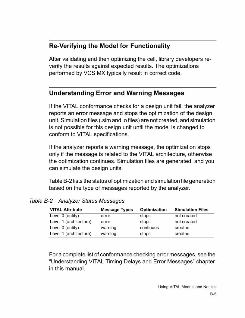
B-5
Using VITAL Models and Netlists
Re-Verifying the Model for Functionality
After validating and then optimizing the cell, library developers re-verify the results against expected results. The optimizations performed by VCS MX typically result in correct code.
Understanding Error and Warning Messages
If the VITAL conformance checks for a design unit fail, the analyzer reports an error message and stops the optimization of the design unit. Simulation files (.sim and .o files) are not created, and simulation is not possible for this design unit until the model is changed to conform to VITAL specifications.
If the analyzer reports a warning message, the optimization stops only if the message is related to the VITAL architecture, otherwise the optimization continues. Simulation files are generated, and you can simulate the design units.
Table B-2 lists the status of optimization and simulation file generation based on the type of messages reported by the analyzer.
Table B-2 Analyzer Status Messages
For a complete list of conformance checking error messages, see the “Understanding VITAL Timing Delays and Error Messages” chapter in this manual.
VITAL Attribute Message Types Optimization Simulation FilesLevel 0 (entity) error stops not createdLevel 1 (architecture) error stops not createdLevel 0 (entity) warning continues createdLevel 1 (architecture) warning stops created
B-6
Using VITAL Models and Netlists
Distributing a VITAL Model
VITAL library developers (usually, ASIC vendors) can distribute models (ASIC library) to designers in any of the following formats:
• A VHDL source file
After conformance checking and verification, you can distribute the cell library in source format. The library is unprotected, but it is portable.
• An encrypted VHDL source file
You can distribute the encrypted file similar to the VHDL source file. Because the encryption algorithms are generally not public and the code is protected, models are not portable to other simulators.
• Simulation files (the .sim and .o files)
The cell is analyzed and optimized by the ASIC vendor. The library is protected and is not portable to other simulators or simulator versions.
For the VHDL file and the encrypted VHDL source file formats, the designer can perform the final compilation to optimize the library object codes by using the -optimize and -event options. ASIC vendors can provide designers with a script specifying the correct compilation procedure.
B-7
Using VITAL Models and Netlists
Simulating a VITAL Netlist
A VITAL-based netlist consists of instances of VITAL cells. There are no VITAL specific or other restrictions on the location of such cells in the netlist, nor are there restrictions regarding the quantity or ratio of such cells in relation to other VHDL descriptions.
To simulate a VITAL netlist, simply invoke scsim.
Applying Stimulus
You apply the input stimulus for the VITAL netlist using the same method and format that you use to apply them for any other netlist, such as using WIF, text input/output, or a testbench.
Overriding Generic Parameter Values
The setup file contains the following three flags that you can use to control the simulation of a VITAL netlist:
• Force_TimingChecksOn_TO
This global flag affects all occurrences of the TimingChecksOn generic in a VITAL cell.
• Force_XOn_TO
This global flag affects all occurrences of the XOn generic in a VITAL cell.
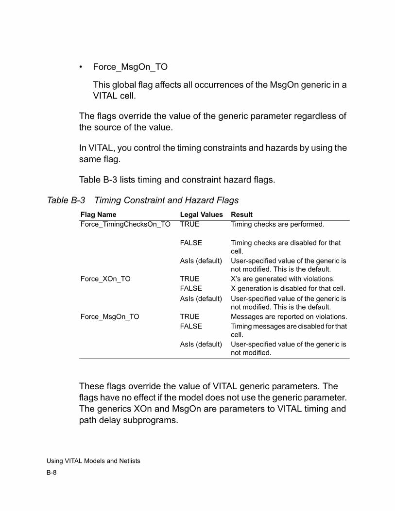
B-8
Using VITAL Models and Netlists
• Force_MsgOn_TO
This global flag affects all occurrences of the MsgOn generic in a VITAL cell.
The flags override the value of the generic parameter regardless of the source of the value.
In VITAL, you control the timing constraints and hazards by using the same flag.
Table B-3 lists timing and constraint hazard flags.
Table B-3 Timing Constraint and Hazard Flags
These flags override the value of VITAL generic parameters. The flags have no effect if the model does not use the generic parameter. The generics XOn and MsgOn are parameters to VITAL timing and path delay subprograms.
Flag Name Legal Values ResultForce_TimingChecksOn_TO TRUE Timing checks are performed.
FALSE Timing checks are disabled for that cell.
AsIs (default) User-specified value of the generic is not modified. This is the default.
Force_XOn_TO TRUE X’s are generated with violations.FALSE X generation is disabled for that cell.AsIs (default) User-specified value of the generic is
not modified. This is the default.Force_MsgOn_TO TRUE Messages are reported on violations.
FALSE Timing messages are disabled for that cell.
AsIs (default) User-specified value of the generic is not modified.
B-9
Using VITAL Models and Netlists
Understanding VCS MX Error Messages
VCS MX reports two types of errors: system errors and model/netlist errors.
System Errors
VCS MX reports a system error if any of the following conditions occur:
• If there are any negative timing values after all timing values are imported and negative constraint calculations (NCC) are performed.
All the adjusted timing values must be positive or zero (>=0) after all timing values are imported and NCC is performed. If an adjusted value is negative, NCC issues a warning message and uses zero instead.
Use the man vss-297 and man vss-298 command to get more information about NCC error messages.
• If you try to “look-into” the parts of the model that are invisible (using the SCL commands, such as ls or cd.)
This is because the visibility is limited in VITAL cells that have been optimized, and the cells are marked as PRIVATE.
Model and Netlist Errors
A VITAL model in a VITAL netlist generates several kinds of errors. The most important are hazard and constraint violations. Both are associated with a violation of the timing model. The format of such errors is defined by the VITAL standard (in VHDL packages.)
B-10
Using VITAL Models and Netlists
Viewing VITAL Subprograms
You cannot view or access VITAL subprograms. The VITAL packages are built-in. Any reference to a VITAL subprogram (functions or procedures) or any other item in the VITAL packages is converted by the analyzer to a built-in representation.
Timing Back-annotation
A VITAL netlist can import timing information from a VHDL configuration or an SDF file.
• A VHDL configuration
VHDL allows the use of a configuration block to override the values of generics specified in the entity declaration. This is done during analysis of the design.
• SDF file
VITAL netlist can import an SDF 2.1 version file. The VITAL standard defines the mapping for SDF 2.1 and the subset supported.
You can back-annotate different versions of SDF files.
- SDF 2.1 files: For VITAL entities with VITAL_Level0 attributes set to TRUE.
- SDF 1.0/ 2.1 files: For other cell type and for back-annotation.
Newly back-annotated values are visible at all times to let you know that back-annotation was successful.
B-11
Using VITAL Models and Netlists
Note:You cannot assign values to the generics of optimized VITAL cells using the assign command.
VCS MX Naming Styles
VCS MX automatically determines what naming style is used according to the cell:
• For conformance checked VITAL cells (that is, VITAL entities with the VITAL_Level0 attribute set to TRUE), VCS MX uses VITAL naming styles.
• For non-VITAL conformance checked cells, VCS MX uses the Synopsys naming style (or the style described in SDF naming file.)
Note:VCS MX ignores the SDFNAMINGSTYLE variable in the setup file when determining the naming style.
Negative Constraints Calculation (NCC)
Adjusting the cell timing values and converting the negative values follows the elaboration and back-annotation phases. VCS MX follows these steps to prepare the design units for simulation:
1. Elaborate design
Elaboration is a VHDL step, the design is created and is ready for the simulation run.
B-12
Using VITAL Models and Netlists
2. Back-annotate timing delay values
Timing values are imported, and the value of generic parameters are updated. VITAL models that support NCC accept backannotation information as in any other cell.
3. Convert the negative constraint values
The value of generic parameters is modified to conform to the NCC algorithm, and negative constraint values are converted to zero or positive.
VCS MX automatically performs NCC only when the VITAL_Level0 attribute is set to TRUE for the VITAL entity and the internal clock delay generic (ticd) or internal signal delay generic (tisd) is set.
VCS MX does not run NCC on design units that have a non-VITAL design type, but you can simulate them.
Note:VCS MX performs NCC after SDF annotation. If you don’t back-annotate the time delays using SDF, NCC is done after elaboration.
4. Run the simulation.
B-13
Using VITAL Models and Netlists
Understanding VITAL Timing Delays and Error Messages
This section describes how VCS MX annotates Standard Delay Format (SDF) data during simulation and how it calculates negative timing constraints during elaboration. This section also lists the error messages that VHDL Analyzer generates while checking design units for VITAL conformance.
This chapter contains the following sections:
• SDF Back-Annotation
• Negative Constraint Calculation (NCC)
• Conformance Checks
• Error Messages
SDF Back-Annotation
The SDF annotator in VCS MX supports the following for VITAL models:
• Mixed versions of SDF files
• Multiple SDF files
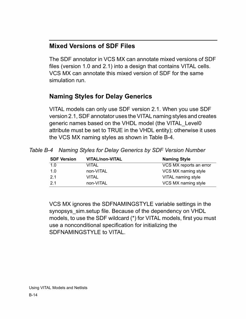
B-14
Using VITAL Models and Netlists
Mixed Versions of SDF Files
The SDF annotator in VCS MX can annotate mixed versions of SDF files (version 1.0 and 2.1) into a design that contains VITAL cells. VCS MX can annotate this mixed version of SDF for the same simulation run.
Naming Styles for Delay Generics
VITAL models can only use SDF version 2.1. When you use SDF version 2.1, SDF annotator uses the VITAL naming styles and creates generic names based on the VHDL model (the VITAL_Level0 attribute must be set to TRUE in the VHDL entity); otherwise it uses the VCS MX naming styles as shown in Table B-4.
Table B-4 Naming Styles for Delay Generics by SDF Version Number
VCS MX ignores the SDFNAMINGSTYLE variable settings in the synopsys_sim.setup file. Because of the dependency on VHDL models, to use the SDF wildcard (*) for VITAL models, first you must use a nonconditional specification for initializing the SDFNAMINGSTYLE to VITAL.
SDF Version VITAL/non-VITAL Naming Style1.0 VITAL VCS MX reports an error1.0 non-VITAL VCS MX naming style2.1 VITAL VITAL naming style2.1 non-VITAL VCS MX naming style

B-15
Using VITAL Models and Netlists
DEVICE Delay
Note:VCS MX supported VITAL version 3.0 timing generic rules beginning with version 3.4b of VCS MX and continues to support it.
The VITAL-SDF name mapping rule for the DEVICE delay is as follows:
tdevice_<InstanceName>[_<OutputPort>]
<InstanceName> is the label for a VITAL primitive concurrent procedure call, and _<OutputPort> is optional.
SDF annotator maps each DEVICE delay into one timing generic.
Example 1:
The SDF entry
(CELL (CELLTYPE ”AN2”)(INSTANCE Top.I1.P2)(DELAY (ABSOLUTE (DEVICE Y (3)(5))))
)
maps to the generic
tdevice_P2_Y
Example 2:
The SDF entry
(CELL (CELLTYPE ”AN2”)(INSTANCE Top.I1.P2)(DELAY (ABSOLUTE (DEVICE (3)(5))))
B-16
Using VITAL Models and Netlists
)
maps to the generic
tdevice_P2
Multiple SDF Files
When you specify multiple SDF files and their switches on the command line, SDF annotator uses the following sequence to apply the switches:
1. Reads and applies the command line switches.
2. Reads the synopsys_sim.setup file.
3. Uses the default values.
For example, if you specify the scsim command for SDF as
scsim -sdf min:/top/blockB/I1:f1.sdf -sdf f2.sdf
and if the synopsys_sim.setup file includes
SDF_TOP = /top/block1
and the default values are
SDF_TOP = NULLSDFINDEX = SDF_TYP
SDF annotator uses the region /top/blockB/I1 and the MIN switches only for the f1.sdf file, and it uses the settings from the synopsys_sim.setup file and the defaults for the f2.sdf file.
B-17
Using VITAL Models and Netlists
Therefore, SDF annotator uses /top/blockB/I1 as the top-level design name and MIN delay for the f1.sdf file. For f2.sdf, it uses /top/block1 as the top-level design name and TYP delay.
SDF Restrictions
When using SDF with VITAL, you must be aware of the following two restrictions:
• SDF port names are not checked.
• VCS MX cannot back-annotate SDF file at run time.
SDF Port Names Not Checked
VCS MX does not check SDF port names against VHDL port names, because VITAL does not require the use of PORT names as the suffix of VITAL generic names. Timing generic names are generated based on delay type and port specification from the SDF file.
Back-Annotation at Elaboration Time
You must back-annotate the SDF file during elaboration and not while you are running simulation. Therefore, you cannot use the include command to invoke the SDF parser for a design that has a VITAL component.
B-18
Using VITAL Models and Netlists
Negative Constraint Calculation (NCC)
VITAL defines the special generics ticd, tisd, tbpd, SignalDelay Block, and equations to adjust the negative setup and hold time and related IOPATH delays.
For VITAL models, NCC adjusts the timing generics for the ticd or tisd generic. The ticd delay is calculated based on SETUP and RECOVERY time. Therefore, NCC resets the original ticd delay in VITAL cells.
Conformance Checks
For VITAL conformance, the analyzer checks the design units that have the VITAL_Level0 or VITAL_Level1 attribute set to TRUE (if the attributes are set to FALSE, the analyzer reports a warning). The only result of the conformance checking from the analyzer is the error messages.
The analyzer performs the following checks:
• Type checking
• Syntactic and Semantic checks
Type Checks
The analyzer checks and verifies the type for generics, restricted variables, timing constraints, delays, and ports.
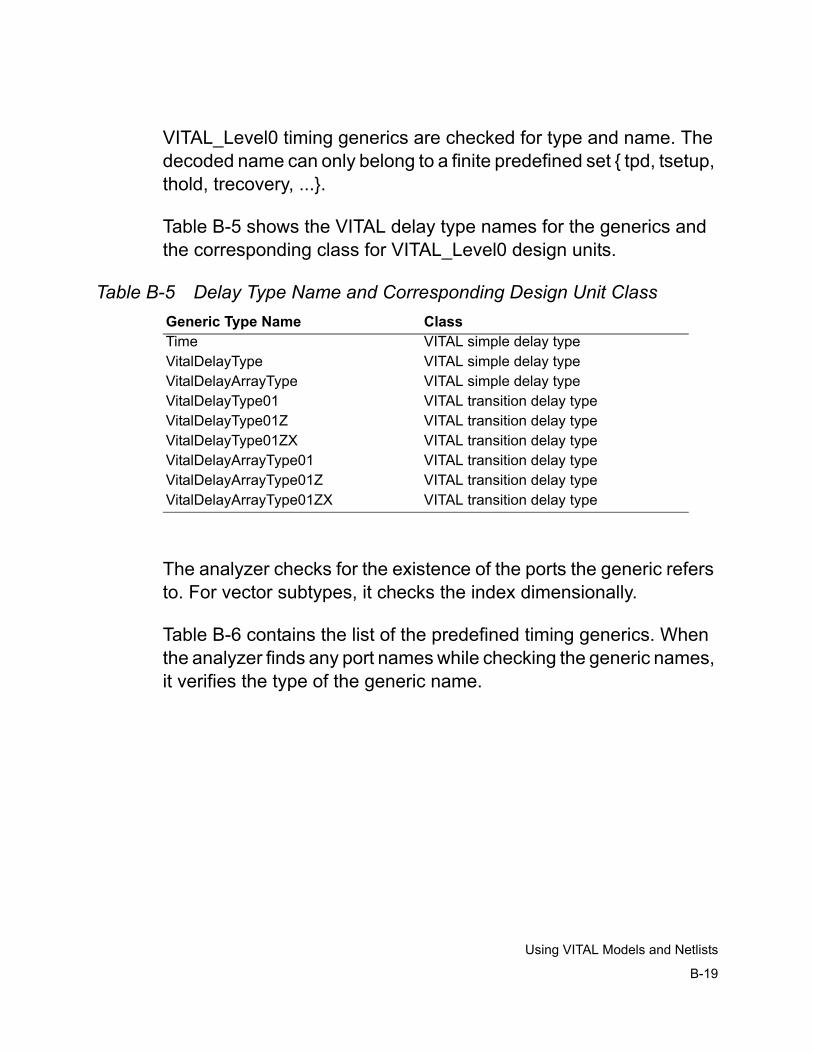
B-19
Using VITAL Models and Netlists
VITAL_Level0 timing generics are checked for type and name. The decoded name can only belong to a finite predefined set { tpd, tsetup, thold, trecovery, ...}.
Table B-5 shows the VITAL delay type names for the generics and the corresponding class for VITAL_Level0 design units.
Table B-5 Delay Type Name and Corresponding Design Unit Class
The analyzer checks for the existence of the ports the generic refers to. For vector subtypes, it checks the index dimensionally.
Table B-6 contains the list of the predefined timing generics. When the analyzer finds any port names while checking the generic names, it verifies the type of the generic name.
Generic Type Name ClassTime VITAL simple delay typeVitalDelayType VITAL simple delay typeVitalDelayArrayType VITAL simple delay typeVitalDelayType01 VITAL transition delay typeVitalDelayType01Z VITAL transition delay typeVitalDelayType01ZX VITAL transition delay typeVitalDelayArrayType01 VITAL transition delay typeVitalDelayArrayType01Z VITAL transition delay typeVitalDelayArrayType01ZX VITAL transition delay type
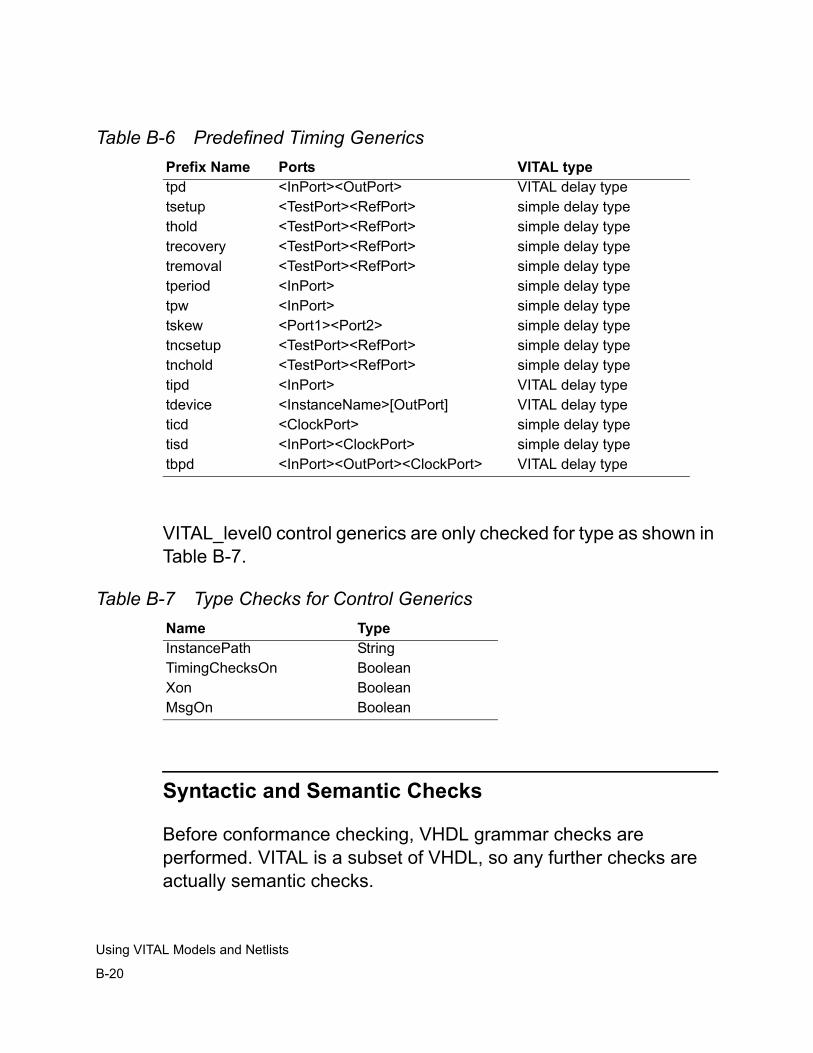
B-20
Using VITAL Models and Netlists
Table B-6 Predefined Timing Generics
VITAL_level0 control generics are only checked for type as shown in Table B-7.
Table B-7 Type Checks for Control Generics
Syntactic and Semantic Checks
Before conformance checking, VHDL grammar checks are performed. VITAL is a subset of VHDL, so any further checks are actually semantic checks.
Prefix Name Ports VITAL typetpd <InPort><OutPort> VITAL delay typetsetup <TestPort><RefPort> simple delay typethold <TestPort><RefPort> simple delay typetrecovery <TestPort><RefPort> simple delay typetremoval <TestPort><RefPort> simple delay typetperiod <InPort> simple delay typetpw <InPort> simple delay typetskew <Port1><Port2> simple delay typetncsetup <TestPort><RefPort> simple delay typetnchold <TestPort><RefPort> simple delay typetipd <InPort> VITAL delay typetdevice <InstanceName>[OutPort] VITAL delay typeticd <ClockPort> simple delay typetisd <InPort><ClockPort> simple delay typetbpd <InPort><OutPort><ClockPort> VITAL delay type
Name TypeInstancePath StringTimingChecksOn BooleanXon BooleanMsgOn Boolean
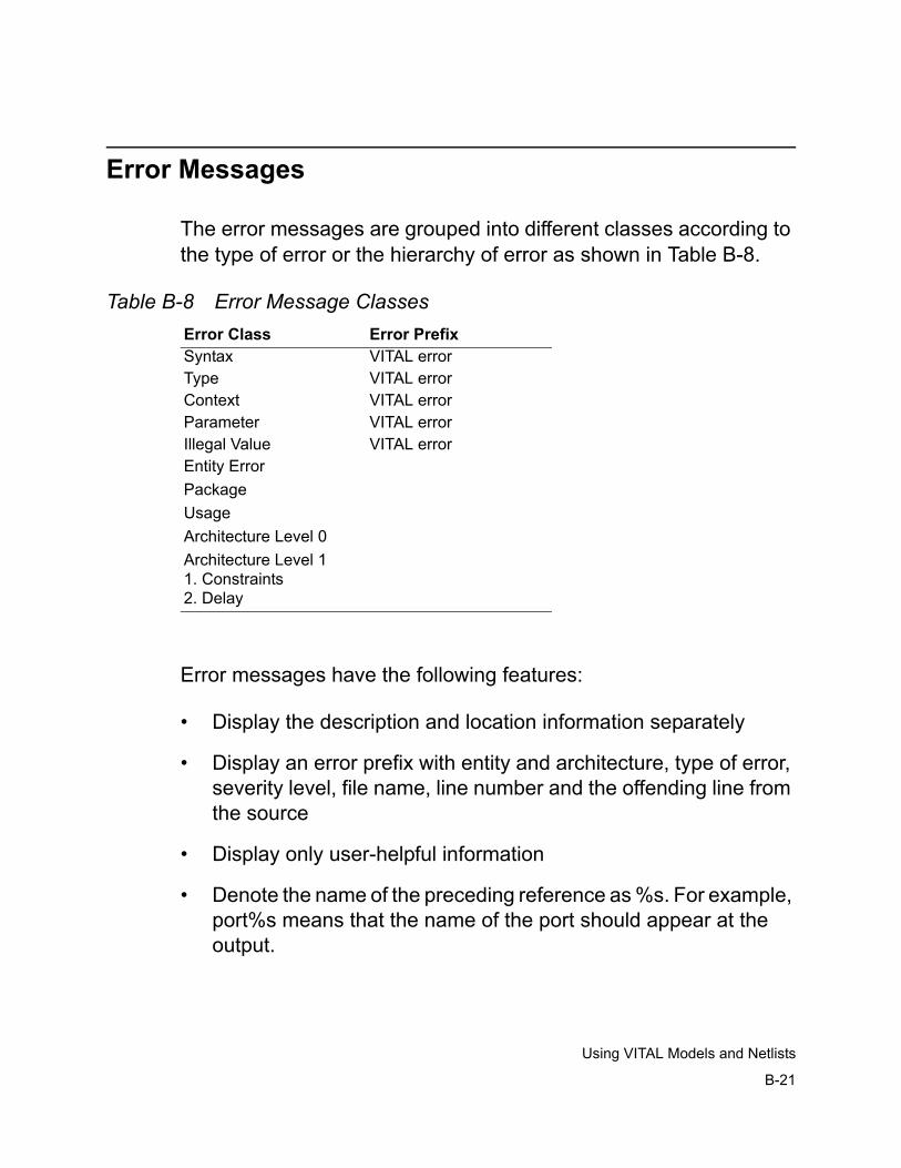
B-21
Using VITAL Models and Netlists
Error Messages
The error messages are grouped into different classes according to the type of error or the hierarchy of error as shown in Table B-8.
Table B-8 Error Message Classes
Error messages have the following features:
• Display the description and location information separately
• Display an error prefix with entity and architecture, type of error, severity level, file name, line number and the offending line from the source
• Display only user-helpful information
• Denote the name of the preceding reference as %s. For example, port%s means that the name of the port should appear at the output.
Error Class Error PrefixSyntax VITAL errorType VITAL errorContext VITAL errorParameter VITAL errorIllegal Value VITAL errorEntity ErrorPackageUsageArchitecture Level 0Architecture Level 11. Constraints2. Delay
B-22
Using VITAL Models and Netlists
• Are one-liners for grep/awk retrieval from the log file
• Are numbered as follows: E-VTL001, W-VTL002, ...
Table B-9 and Table B-10 list all the VITAL error messages. Every message is prefixed with an error class specific message and sufficient context for you to find the problem object. For example, if a port is the offending object, the name of the port and entity are provided. For type violation, the offending type is shown. When there is no indication of what was found, it means that the negation of the statement was found. For example, the error message “The actual part of ... MUST be static” indicates that the type found is not static.
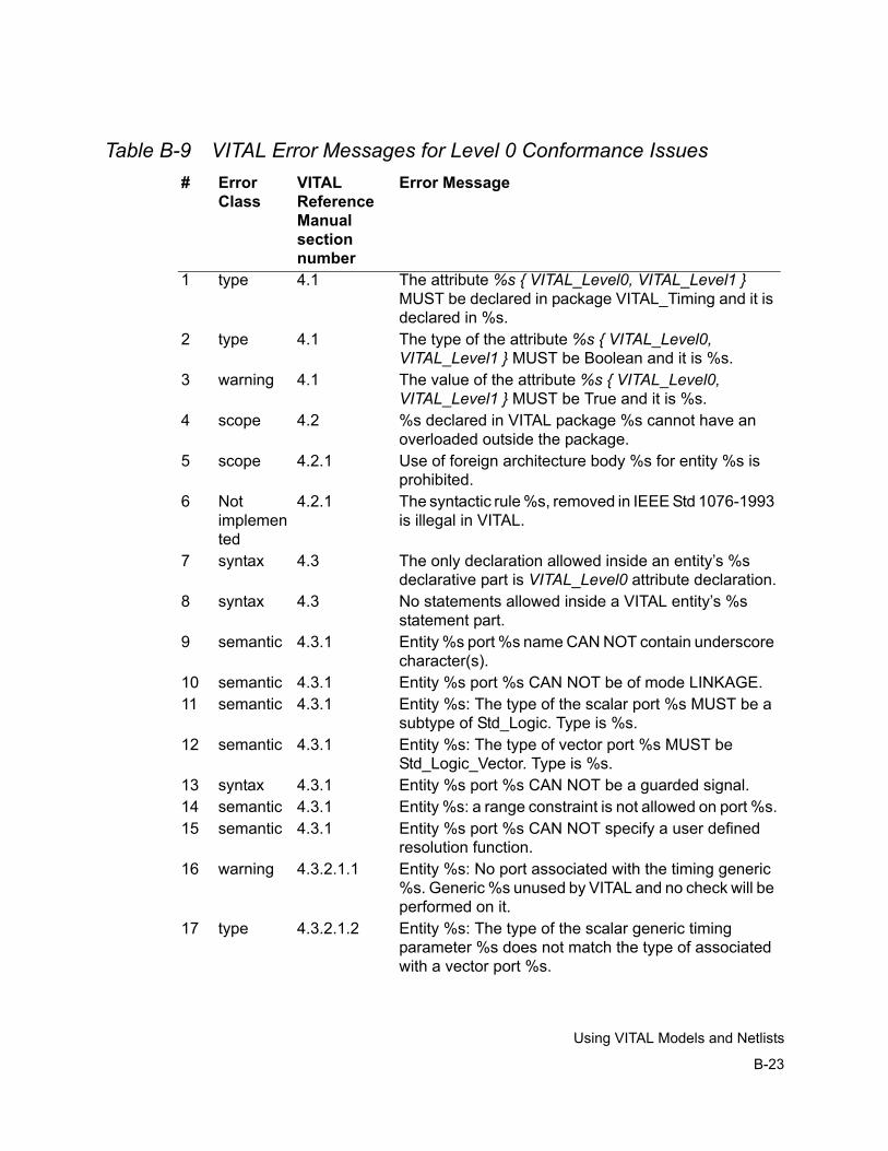
B-23
Using VITAL Models and Netlists
Table B-9 VITAL Error Messages for Level 0 Conformance Issues# Error
Class VITAL Reference Manual section number
Error Message
1 type 4.1 The attribute %s { VITAL_Level0, VITAL_Level1 } MUST be declared in package VITAL_Timing and it is declared in %s.
2 type 4.1 The type of the attribute %s { VITAL_Level0, VITAL_Level1 } MUST be Boolean and it is %s.
3 warning 4.1 The value of the attribute %s { VITAL_Level0, VITAL_Level1 } MUST be True and it is %s.
4 scope 4.2 %s declared in VITAL package %s cannot have an overloaded outside the package.
5 scope 4.2.1 Use of foreign architecture body %s for entity %s is prohibited.
6 Not implemented
4.2.1 The syntactic rule %s, removed in IEEE Std 1076-1993 is illegal in VITAL.
7 syntax 4.3 The only declaration allowed inside an entity’s %s declarative part is VITAL_Level0 attribute declaration.
8 syntax 4.3 No statements allowed inside a VITAL entity’s %s statement part.
9 semantic 4.3.1 Entity %s port %s name CAN NOT contain underscore character(s).
10 semantic 4.3.1 Entity %s port %s CAN NOT be of mode LINKAGE.11 semantic 4.3.1 Entity %s: The type of the scalar port %s MUST be a
subtype of Std_Logic. Type is %s.12 semantic 4.3.1 Entity %s: The type of vector port %s MUST be
Std_Logic_Vector. Type is %s.13 syntax 4.3.1 Entity %s port %s CAN NOT be a guarded signal.14 semantic 4.3.1 Entity %s: a range constraint is not allowed on port %s.15 semantic 4.3.1 Entity %s port %s CAN NOT specify a user defined
resolution function.16 warning 4.3.2.1.1 Entity %s: No port associated with the timing generic
%s. Generic %s unused by VITAL and no check will be performed on it.
17 type 4.3.2.1.2 Entity %s: The type of the scalar generic timing parameter %s does not match the type of associated with a vector port %s.
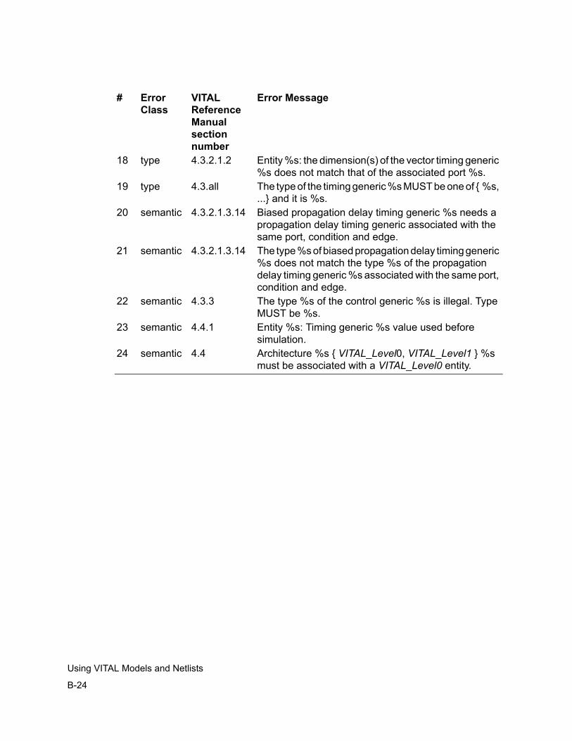
B-24
Using VITAL Models and Netlists
18 type 4.3.2.1.2 Entity %s: the dimension(s) of the vector timing generic %s does not match that of the associated port %s.
19 type 4.3.all The type of the timing generic %s MUST be one of { %s, ...} and it is %s.
20 semantic 4.3.2.1.3.14 Biased propagation delay timing generic %s needs a propagation delay timing generic associated with the same port, condition and edge.
21 semantic 4.3.2.1.3.14 The type %s of biased propagation delay timing generic %s does not match the type %s of the propagation delay timing generic %s associated with the same port, condition and edge.
22 semantic 4.3.3 The type %s of the control generic %s is illegal. Type MUST be %s.
23 semantic 4.4.1 Entity %s: Timing generic %s value used before simulation.
24 semantic 4.4 Architecture %s { VITAL_Level0, VITAL_Level1 } %s must be associated with a VITAL_Level0 entity.
# Error Class
VITAL Reference Manual section number
Error Message
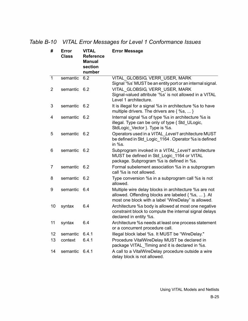
B-25
Using VITAL Models and Netlists
Table B-10 VITAL Error Messages for Level 1 Conformance Issues# Error
ClassVITAL Reference Manual section number
Error Message
1 semantic 6.2 VITAL_GLOBSIG, VERR_USER, MARKSignal ’%s’ MUST be an entity port or an internal signal.
2 semantic 6.2 VITAL_GLOBSIG, VERR_USER, MARKSignal-valued attribute ’%s’ is not allowed in a VITAL Level 1 architecture.
3 semantic 6.2 It is illegal for a signal %s in architecture %s to have multiple drivers. The drivers are { %s, ... }
4 semantic 6.2 Internal signal %s of type %s in architecture %s is illegal. Type can be only of type { Std_ULogic, StdLogic_Vector }. Type is %s.
5 semantic 6.2 Operators used in a VITAL_Level1 architecture MUST be defined in Std_Logic_1164 . Operator %s is defined in %s.
6 semantic 6.2 Subprogram invoked in a VITAL_Level1 architecture MUST be defined in Std_Logic_1164 or VITAL package. Subprogram %s is defined in %s.
7 semantic 6.2 Formal subelement association %s in a subprogram call %s is not allowed.
8 semantic 6.2 Type conversion %s in a subprogram call %s is not allowed.
9 semantic 6.4 Multiple wire delay blocks in architecture %s are not allowed. Offending blocks are labeled { %s, ... }. At most one block with a label “WireDelay” is allowed.
10 syntax 6.4 Architecture %s body is allowed at most one negative constraint block to compute the internal signal delays declared in entity %s.
11 syntax 6.4 Architecture %s needs at least one process statement or a concurrent procedure call.
12 semantic 6.4.1 Illegal block label %s. It MUST be “WireDelay."13 context 6.4.1 Procedure VitalWireDelay MUST be declared in
package VITAL_Timing and it is declared in %s.14 semantic 6.4.1 A call to a VitalWireDelay procedure outside a wire
delay block is not allowed.
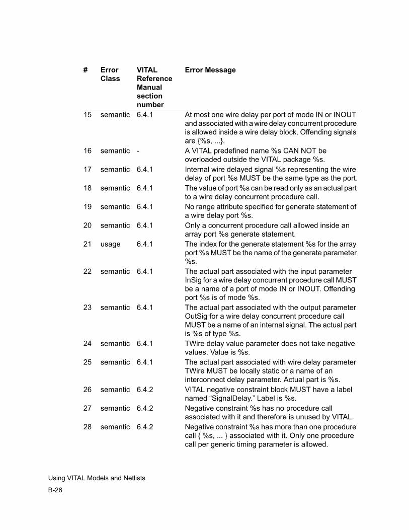
B-26
Using VITAL Models and Netlists
15 semantic 6.4.1 At most one wire delay per port of mode IN or INOUT and associated with a wire delay concurrent procedure is allowed inside a wire delay block. Offending signals are {%s, ...}.
16 semantic - A VITAL predefined name %s CAN NOT be overloaded outside the VITAL package %s.
17 semantic 6.4.1 Internal wire delayed signal %s representing the wire delay of port %s MUST be the same type as the port.
18 semantic 6.4.1 The value of port %s can be read only as an actual part to a wire delay concurrent procedure call.
19 semantic 6.4.1 No range attribute specified for generate statement of a wire delay port %s.
20 semantic 6.4.1 Only a concurrent procedure call allowed inside an array port %s generate statement.
21 usage 6.4.1 The index for the generate statement %s for the array port %s MUST be the name of the generate parameter %s.
22 semantic 6.4.1 The actual part associated with the input parameter InSig for a wire delay concurrent procedure call MUST be a name of a port of mode IN or INOUT. Offending port %s is of mode %s.
23 semantic 6.4.1 The actual part associated with the output parameter OutSig for a wire delay concurrent procedure call MUST be a name of an internal signal. The actual part is %s of type %s.
24 semantic 6.4.1 TWire delay value parameter does not take negative values. Value is %s.
25 semantic 6.4.1 The actual part associated with wire delay parameter TWire MUST be locally static or a name of an interconnect delay parameter. Actual part is %s.
26 semantic 6.4.2 VITAL negative constraint block MUST have a label named “SignalDelay.” Label is %s.
27 semantic 6.4.2 Negative constraint %s has no procedure call associated with it and therefore is unused by VITAL.
28 semantic 6.4.2 Negative constraint %s has more than one procedure call { %s, ... } associated with it. Only one procedure call per generic timing parameter is allowed.
# Error Class
VITAL Reference Manual section number
Error Message
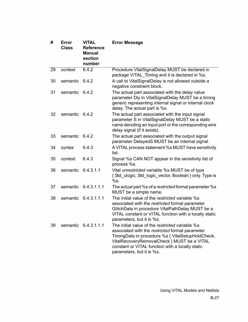
B-27
Using VITAL Models and Netlists
29 context 6.4.2 Procedure VitalSignalDelay MUST be declared in package VITAL_Timing and it is declared in %s.
30 semantic 6.4.2 A call to VitalSignalDelay is not allowed outside a negative constraint block.
31 semantic 6.4.2 The actual part associated with the delay value parameter Dly in VitalSignalDelay MUST be a timing generic representing internal signal or internal clock delay. The actual part is %s.
32 semantic 6.4.2 The actual part associated with the input signal parameter S in VitalSignalDelay MUST be a static name denoting an input port or the corresponding wire delay signal (if it exists).
33 semantic 6.4.2 The actual part associated with the output signal parameter DelayedS MUST be an internal signal.
34 syntax 6.4.3 A VITAL process statement %s MUST have sensitivity list.
35 context 6.4.3 Signal %s CAN NOT appear in the sensitivity list of process %s.
36 semantic 6.4.3.1.1 Vital unrestricted variable %s MUST be of type { Std_ulogic, Std_logic_vector, Boolean } only. Type is %s.
37 semantic 6.4.3.1.1.1 The actual part %s of a restricted formal parameter %s MUST be a simple name.
38 semantic 6.4.3.1.1.1 The initial value of the restricted variable %s associated with the restricted formal parameter GlitchData in procedure VitalPathDelay MUST be a VITAL constant or VITAL function with a locally static parameters, but it is %s.
39 semantic 6.4.3.1.1.1 The initial value of the restricted variable %s associated with the restricted formal parameter TimingData in procedure %s { VitalSetupHoldCheck, VitalRecoveryRemovalCheck } MUST be a VITAL constant or VITAL function with a locally static parameters, but it is %s.
# Error Class
VITAL Reference Manual section number
Error Message
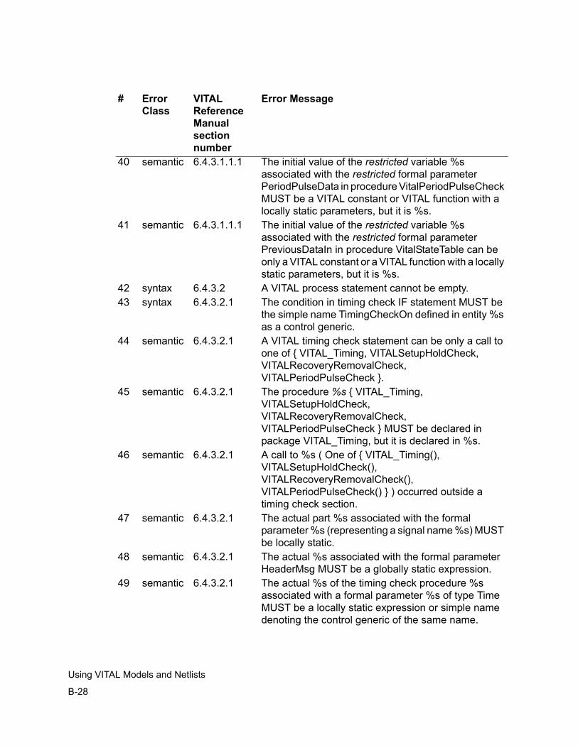
B-28
Using VITAL Models and Netlists
40 semantic 6.4.3.1.1.1 The initial value of the restricted variable %s associated with the restricted formal parameter PeriodPulseData in procedure VitalPeriodPulseCheck MUST be a VITAL constant or VITAL function with a locally static parameters, but it is %s.
41 semantic 6.4.3.1.1.1 The initial value of the restricted variable %s associated with the restricted formal parameter PreviousDataIn in procedure VitalStateTable can be only a VITAL constant or a VITAL function with a locally static parameters, but it is %s.
42 syntax 6.4.3.2 A VITAL process statement cannot be empty.43 syntax 6.4.3.2.1 The condition in timing check IF statement MUST be
the simple name TimingCheckOn defined in entity %s as a control generic.
44 semantic 6.4.3.2.1 A VITAL timing check statement can be only a call to one of { VITAL_Timing, VITALSetupHoldCheck, VITALRecoveryRemovalCheck, VITALPeriodPulseCheck }.
45 semantic 6.4.3.2.1 The procedure %s { VITAL_Timing, VITALSetupHoldCheck, VITALRecoveryRemovalCheck, VITALPeriodPulseCheck } MUST be declared in package VITAL_Timing, but it is declared in %s.
46 semantic 6.4.3.2.1 A call to %s ( One of { VITAL_Timing(), VITALSetupHoldCheck(), VITALRecoveryRemovalCheck(), VITALPeriodPulseCheck() } ) occurred outside a timing check section.
47 semantic 6.4.3.2.1 The actual part %s associated with the formal parameter %s (representing a signal name %s) MUST be locally static.
48 semantic 6.4.3.2.1 The actual %s associated with the formal parameter HeaderMsg MUST be a globally static expression.
49 semantic 6.4.3.2.1 The actual %s of the timing check procedure %s associated with a formal parameter %s of type Time MUST be a locally static expression or simple name denoting the control generic of the same name.
# Error Class
VITAL Reference Manual section number
Error Message

B-29
Using VITAL Models and Netlists
50 semantic 6.4.3.2.1 The actual %s associated with a formal parameter %s { XOn, MsgOn } MUST be a globally static expression.
51 semantic 6.4.3.2.1 A function %s call or an operator %s invocation in the actual part to a formal parameter %s MUST be a function/operator defined in one of packages { Standard, Std_logic_1164, VITAL_Timing }.
52 semantic 6.4.3.2.1 The actual %s associated with the formal parameter %s { TestSignalName } MUST be locally static expression.
53 context 6.4.3.2.1 variable %s associated with a timing check violation parameter %s could not be used in another timing check statement. It appears in timing check %s.
54 context 6.4.3.2.2 procedure VitalStateTable() MUST be declared in the package VITAL_Primitives, but it is declared in %s.
55 semantic 6.4.3.2.2 Only a call to the predefined procedure VitalStateTable() is allowed inside a VITAL functionality section.
56 semantic 6.4.3.2.2 The actual %s associated with the StateTable parameter to procedure VitalStateTable MUST be globally static expression.
57 semantic 6.4.3.2.2 The index constraint on the variable %s associated with the PreviousDataIn parameter MUST match the constraint on the actual associated with the DataIn parameter.
58 semantic 6.4.3.2.2 The target of a VITAL variable assignment MUST be unrestricted variable denoted by a locally static name, but it is %s.
59 type 6.4.3.2.2 The target of an assignment statement of a standard logic type inside a functionality section requires a primary on the right side to be one of the following:1. A globally static expression2. A name of a port or an internal signal3. A function call to a standard logic function, a VITAL primitive or VITALTruthTable()4. An aggregate or a qualified expression with an aggregate operand5. A parenthesized expression
# Error Class
VITAL Reference Manual section number
Error Message
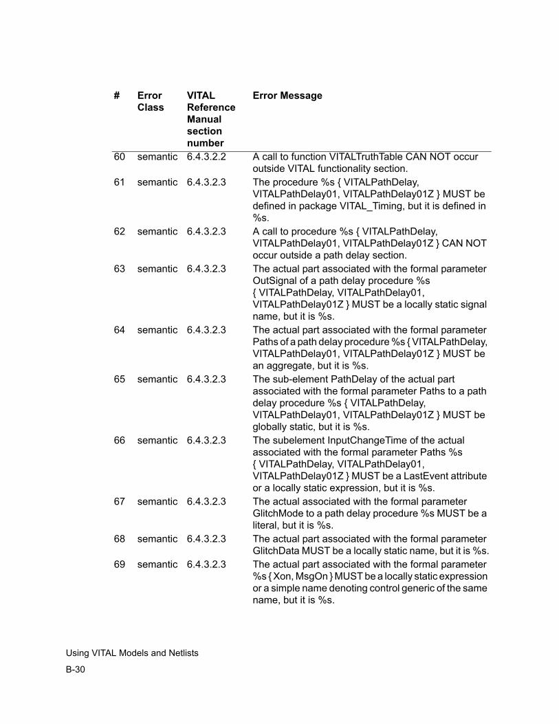
B-30
Using VITAL Models and Netlists
60 semantic 6.4.3.2.2 A call to function VITALTruthTable CAN NOT occur outside VITAL functionality section.
61 semantic 6.4.3.2.3 The procedure %s { VITALPathDelay, VITALPathDelay01, VITALPathDelay01Z } MUST be defined in package VITAL_Timing, but it is defined in %s.
62 semantic 6.4.3.2.3 A call to procedure %s { VITALPathDelay, VITALPathDelay01, VITALPathDelay01Z } CAN NOT occur outside a path delay section.
63 semantic 6.4.3.2.3 The actual part associated with the formal parameter OutSignal of a path delay procedure %s { VITALPathDelay, VITALPathDelay01, VITALPathDelay01Z } MUST be a locally static signal name, but it is %s.
64 semantic 6.4.3.2.3 The actual part associated with the formal parameter Paths of a path delay procedure %s { VITALPathDelay, VITALPathDelay01, VITALPathDelay01Z } MUST be an aggregate, but it is %s.
65 semantic 6.4.3.2.3 The sub-element PathDelay of the actual part associated with the formal parameter Paths to a path delay procedure %s { VITALPathDelay, VITALPathDelay01, VITALPathDelay01Z } MUST be globally static, but it is %s.
66 semantic 6.4.3.2.3 The subelement InputChangeTime of the actual associated with the formal parameter Paths %s { VITALPathDelay, VITALPathDelay01, VITALPathDelay01Z } MUST be a LastEvent attribute or a locally static expression, but it is %s.
67 semantic 6.4.3.2.3 The actual associated with the formal parameter GlitchMode to a path delay procedure %s MUST be a literal, but it is %s.
68 semantic 6.4.3.2.3 The actual part associated with the formal parameter GlitchData MUST be a locally static name, but it is %s.
69 semantic 6.4.3.2.3 The actual part associated with the formal parameter %s { Xon, MsgOn } MUST be a locally static expression or a simple name denoting control generic of the same name, but it is %s.
# Error Class
VITAL Reference Manual section number
Error Message

B-31
Using VITAL Models and Netlists
70 semantic 6.4.3.2.3 The actual part associated with the formal parameter %s { OutSignalName, DefaultDelay, OutputMap } MUST be a locally static expression.
71 No Check 6.4.3.2.3 Port of type %s { OUT, INOUT, BUFFER } has to be driven by a VITAL primitive procedure call or a path delay procedure, but the driver is %s.
72 semantic 6.4.4 The actual associated with the formal parameter %s of class VARIABLE or SIGNAL on VITAL primitive %s MUST be a static name, but it is %s.
73 semantic 6.4.4 The actual part associated with the formal parameter %s of class CONSTANT to a procedure call %s MUST be a locally static expression, but it is %s.
74 semantic 6.4.4 The actual part associated with the formal parameter ResultMap to a procedure call %s MUST be a locally static expression, but it is %s.
75 semantic 6.4.4 The actual part associated with the formal parameter %s { TruthTable, StateTable } on table primitive procedure call %s MUST be a constant whose value expression is an aggregate with fields that are locally static expressions.
76 No Check 7.1.1 VITAL logic primitive %s MUST be defined in package %s.
77 No Check 7.3.1 Symbol %s CAN NOT appear in Table %s.78 No Check 7.3.3.1 Wrong number of inputs to an object %s of type
VitalTruthTable. The number MUST equal to the value of the DataIn parameter VitalTruthTable.
79 No Check 7.3.3.1 Wrong dimensions for table %s of type %s { VitalTruthTable, VitalStateTable }.
80 Package 7.4.3.2.2 procedure VitalStateTable() MUST be declared in VitalPrimitives, but it is declared in %s.
81 Package 7.4.3.2.3 procedure %s { VITALPathDelay, VITALPathDelay01, VITALPathDelay01Z } MUST be defined in package VITAL_Timing, but it is defined in %s.
# Error Class
VITAL Reference Manual section number
Error Message

B-32
Using VITAL Models and Netlists
C-1
SAIF Support
CSAIF Support C
You can do power analysis and power optimization using the Synopsys Power Compiler by entering the power command from the simulator prompt. This command outputs Switching Activity Interchange Format (SAIF) files for your design.
Signals and ports are supported for monitoring as well as constructs such as generates, enumerated types, records, array of arrays, and integers.
Using SAIF files with VCS MX
Note the following when using SAIF files with VCS/VCS MX in the new flow:
• No additional switches are necessary for VCS/VCS MX.
• A Power Compiler specific tab file (and the corresponding library) does not need to be provided to VCS.
• No additional settings are needed for VCS/VCS MX.
C-2
SAIF Support
• Functionality is built-in to VCS and VCS MX.
If you want to switch to the old flow of dumping SAIF files with the PLI, you can continue to give "-P $VPOWER_TAB $VPOWER_LIB" to VCS, and the flow will not use the native support. So, just by removing the PLI-related SAIF arguments from VCS command line, you can switch to native SAIF support in VCS.
SAIF Calls that can be Used on Verilog or Verilog-Top Designs
This section describes SAIF calls that can be used at the Verilog or VCS-CLI prompt.
Note that mixedHdlScope in the following discussion can be one of the following:
• Verilog scope
• VHDL scope
• Mixed HDL scope
Note also that a design_object in the following discussion can be one of the following:
• Verilog scope or variable
• VHDL scope or variable
• Any MixedHDL scope or variable)
$set_toggle_region
Allows you to define an object or a scope region for which the switching activity needs to be reported.
Syntax:
$set_toggle_region(design_obj [, design_object]);
C-3
SAIF Support
$toggle_start
Instructs the simulator to start monitoring switching activity.
Syntax:
$toggle_start();
$toggle_stop
Instructs the simulator to stop monitoring switching activity.
Syntax
$toggle_stop();
$toggle_reset
This command sets the toggle counter to 0 for all the nets in the current toggle region.
Syntax:
$toggle_reset();
$toggle_report
Reports switching activity to an output file.
Syntax:
$toggle_report(<outputFile>, synthesisTimeUnit, <mixedHdlScope>);
This task has a slight change in native SAIF implementation compared to PLI-based implementation. Only the arguments specified here will be considered for processing. Other arguments have no meaning.
C-4
SAIF Support
$read_lib_saif
Allows you to read in a SDPD library forward SAIF file. It registers the state and path dependent information on the scope. It also turns on monitor on internal nets of the design.
Syntax:
$read_lib_saif(<inputFile>);
$read_rtl_saif
Allows the user to read in an RTL forward SAIF file. It registers synthesis invarient elements by reading forward SAIF file. By default, it doesn't register internal nets. If neither $read_lib_saif nor $read_rtl_saif is specified, then also all the internal nets will be monitored.
Syntax:
$read_rtl_saif(<inputFile>, [, testbench_path_name]);
$set_gate_level_monitoring
Allows the user to turn on/off the monitoring of nets in the design if both $read_lib_saif and $read_rtl_saif are present in the design.
Syntax:
$set_gate_level_monitoring("on" | "off" | "rtl_on");
"rtl_on": All reg type of objects are monitored for toggles. Net type of objects are monitored only if it is a cell highconn. This is the
default monitoring policy.
"off": net type of objects are not monitored.
"on": reg type of objects are monitored only if it is a cell hiconn.
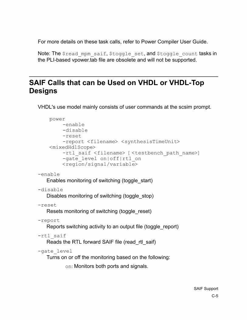
C-5
SAIF Support
For more details on these task calls, refer to Power Compiler User Guide.
Note: The $read_mpm_saif, $toggle_set, and $toggle_count tasks in the PLI-based vpower.tab file are obsolete and will not be supported.
SAIF Calls that can be Used on VHDL or VHDL-Top Designs
VHDL's use model mainly consists of user commands at the scsim prompt.
power-enable-disable-reset-report <filename> <synthesisTimeUnit>
<mixedHdlScope>-rtl_saif <filename> [<testbench_path_name>]-gate_level on|off|rtl_on<region/signal/variable>
-enableEnables monitoring of switching (toggle_start)
-disableDisables monitoring of switching (toggle_stop)
-resetResets monitoring of switching (toggle_reset)
-reportReports switching activity to an output file (toggle_report)
-rtl_saifReads the RTL forward SAIF file (read_rtl_saif)
-gate_levelTurns on or off the monitoring based on the following:
on: Monitors both ports and signals.
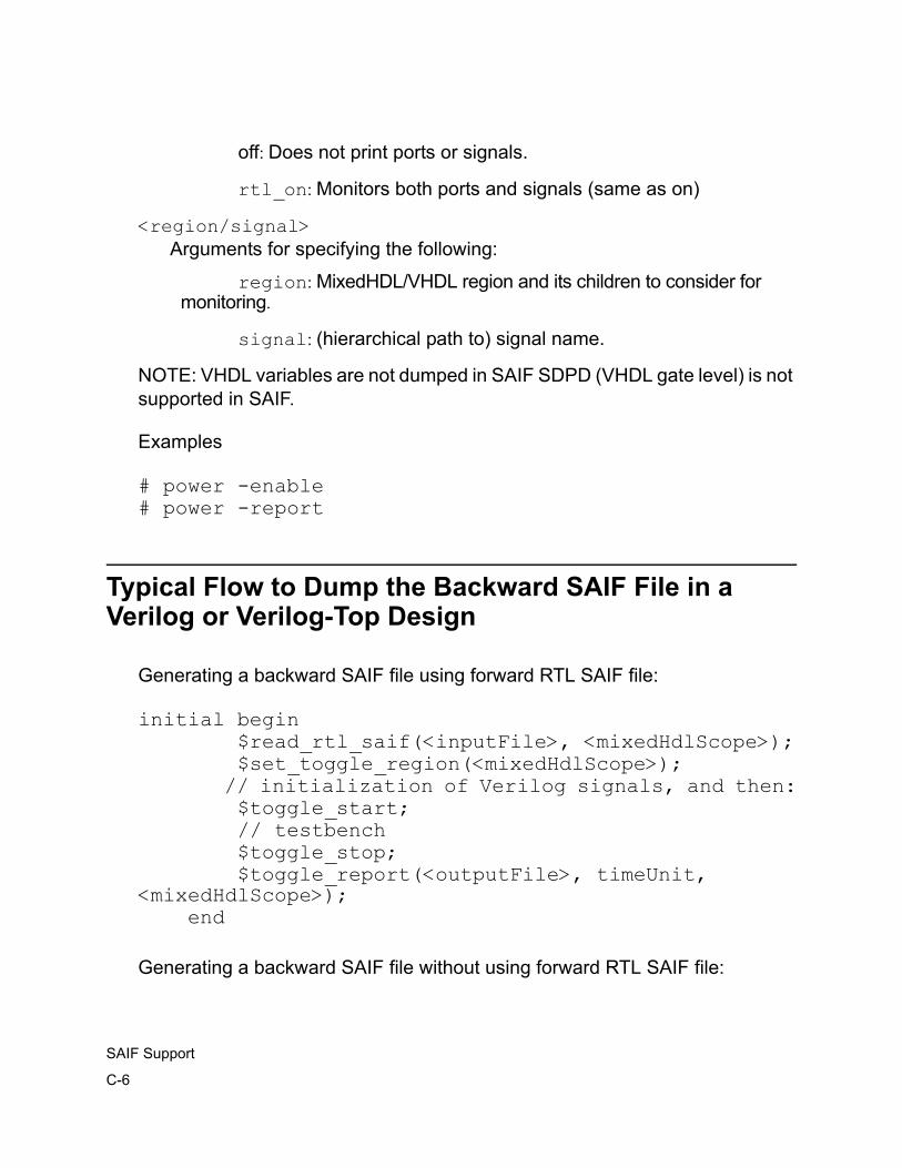
C-6
SAIF Support
off: Does not print ports or signals.
rtl_on: Monitors both ports and signals (same as on)
<region/signal>Arguments for specifying the following:
region: MixedHDL/VHDL region and its children to consider for monitoring.
signal: (hierarchical path to) signal name.
NOTE: VHDL variables are not dumped in SAIF SDPD (VHDL gate level) is not supported in SAIF.
Examples
# power -enable# power -report
Typical Flow to Dump the Backward SAIF File in a Verilog or Verilog-Top Design
Generating a backward SAIF file using forward RTL SAIF file:
initial begin $read_rtl_saif(<inputFile>, <mixedHdlScope>); $set_toggle_region(<mixedHdlScope>); // initialization of Verilog signals, and then: $toggle_start; // testbench $toggle_stop; $toggle_report(<outputFile>, timeUnit, <mixedHdlScope>); end
Generating a backward SAIF file without using forward RTL SAIF file:
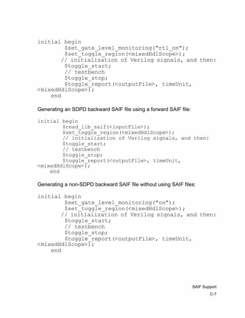
C-7
SAIF Support
initial begin $set_gate_level_monitoring("rtl_on"); $set_toggle_region(<mixedHdlScope>); // initialization of Verilog signals, and then: $toggle_start; // testbench $toggle_stop; $toggle_report(<outputFile>, timeUnit, <mixedHdlScope>); end
Generating an SDPD backward SAIF file using a forward SAIF file:
initial begin $read_lib_saif(<inputFile>); $set_toggle_region(<mixedHdlScope>); // initialization of Verilog signals, and then: $toggle_start; // testbench $toggle_stop; $toggle_report(<outputFile>, timeUnit, <mixedHdlScope>); end
Generating a non-SDPD backward SAIF file without using SAIF files:
initial begin $set_gate_level_monitoring("on"); $set_toggle_region(<mixedHdlScope>); // initialization of Verilog signals, and then: $toggle_start; // testbench $toggle_stop; $toggle_report(<outputFile>, timeUnit, <mixedHdlScope>); end
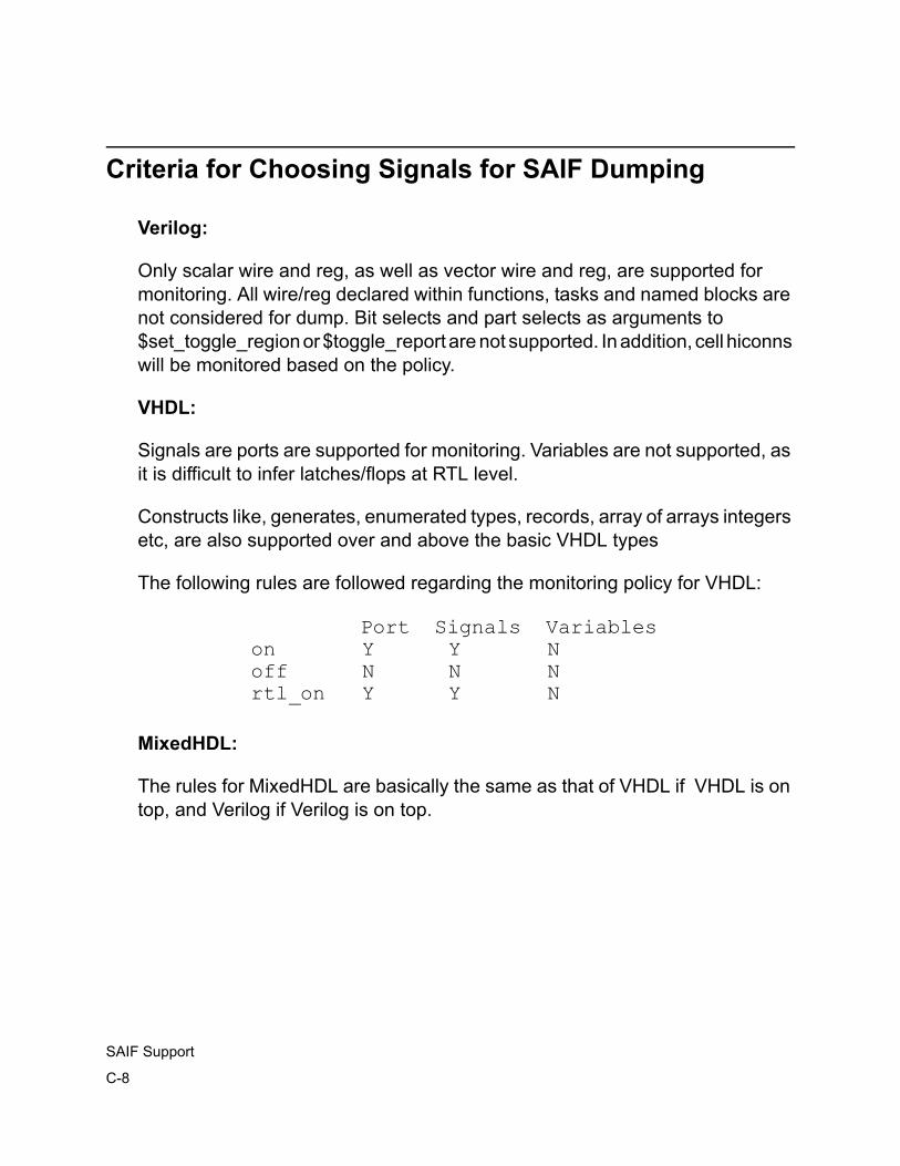
C-8
SAIF Support
Criteria for Choosing Signals for SAIF Dumping
Verilog:
Only scalar wire and reg, as well as vector wire and reg, are supported for monitoring. All wire/reg declared within functions, tasks and named blocks are not considered for dump. Bit selects and part selects as arguments to $set_toggle_region or $toggle_report are not supported. In addition, cell hiconns will be monitored based on the policy.
VHDL:
Signals are ports are supported for monitoring. Variables are not supported, as it is difficult to infer latches/flops at RTL level.
Constructs like, generates, enumerated types, records, array of arrays integers etc, are also supported over and above the basic VHDL types
The following rules are followed regarding the monitoring policy for VHDL:
Port Signals Variables on Y Y N off N N N rtl_on Y Y N
MixedHDL:
The rules for MixedHDL are basically the same as that of VHDL if VHDL is on top, and Verilog if Verilog is on top.
C-9
SAIF Support
TCL File for MTI Users to Convert Existing SAIF UI Commands
If you are an MTI user, you can source a TCL file so that you don't have to convert your existing SAIF UI commands to VCS MX "power" commands.
The script, named "cmdPower.tcl", is installed in the following location:
$VCS_HOME/etc/miscTo use this TCL file and have access to all MTI power commands, enter the following command at the scsim prompt:
source cmdPower.tcl

C-10
SAIF Support
D-1
Using VCS MX ESI Adapter
DUsing VCS MX ESI Adapter A
VCS MX ESI Adapter integrates VCS-MX with the Specman Elite Release 4.2.1 with the ESI interface. This appendix describes how to prepare a stand-alone VHDL design or mixed VHDL/ Verilog design for use with the ESI interface. Please refer to the Specman Elite User Guide for further information.
Note that Specman is implemented as a VHPI foreign architecture. So, a VHDL stub file called specman.vhd is provided as part of VCS MX release. It has to be instantiated in the DUT, and you will need to anlayze the file explicitly.
This appendix covers the following topics:
• Type Support
• Usage Flow
D-2
Using VCS MX ESI Adapter
Type Support
The VCS MX ESI adapter supports the following VHDL types:
• Predefined types
- bit
- boolean
- std_logic/std_ulogic
- character
• User-defined enum types
• in/out/inout/buffer ports
• Access to elements of the following composite types supported:
- Access to individual elements of any of the supported scalar types
- Predefined types based on any of the supported scalar types such as string, bit_vector, integer, etc.
The VCS MX ESI adapter supports the following Verilog Types • nets
• wires
• registers
• integers
• array of registers (verilog memory)
Using VCS MX ESI AdapterD-3
Other Verilog support:
• Verilog macros
• Verilog tasks
• Verilog functions
• Verilog events
• in/out/inout ports
Usage Flow
The Specman usage model for VCS MX depends upon whether e code can access both VHDL and Verilog, or just one language. If e code can access just one language, then you don't have to specify the unused part.
Setting Up to Run Specman with VCS MX
This section describes how to set up your enviornment to run Specman with VCS MX:
1. Set your VCS_HOME and SPECMAN_HOME environment variables:
$ setenv VCS_HOME <vcs mx installation> $ setenv SPECMAN_HOME <specman installation>
2. Source you env.csh file for Specman:
source ${SPECMAN_HOME}/env.csh

D-4
Using VCS MX ESI Adapter
3. Set your environment for the VCS MX Specman ESI adapter:
- In 7.0.x releases:
% setenv SPECMAN_VCSMX_VHDL_ADAPTER $VCS_HOME/$ARCH/sim/lib/libvhdl_sn_adapter.so
- In in 7.1.x releases:
$ setenv SPECMAN_VCSMX_VHDL_ADAPTER ${VCS_HOME}/${ARCH}/lib/libvhdl_sn_adapter.so
4. Set your environment to run e code in loaded mode (default mode):
$ setenv SPECMAN_DLIB ${SPECMAN_HOME}/`${SPECMAN_HOME}/bin/sn_arch.sh`/libspecman.so
or set your environment to run run e code in compiled mode:
% $SPECMAN_HOME/bin/sn_compile.sh -shlib xor_verify% setenv SPECMAN_DLIB `pwd`/libsn_<xor_verify>.so
Note that VCS MX Specman ESI adapter is implemented as a vhpi foreign architecture. So, a VHDL stub file called 'specman.vhd' is provided as part of VCS MX release. It has to be instantiated in DUT and user needs to anlayze the file explicitly. The file is located under your VCS MX installation ($VCS_HOME/packages/synopsys/src/specman.vhd)
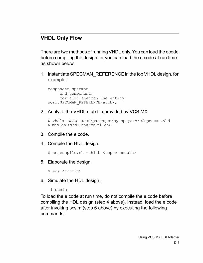
Using VCS MX ESI AdapterD-5
VHDL Only Flow
There are two methods of running VHDL only. You can load the ecode before compiling the design. or you can load the e code at run time. as shown below.
1. Instantiate SPECMAN_REFERENCE in the top VHDL design, for example:
component specman end component; for all: specman use entity work.SPECMAN_REFERENCE(arch);
2. Analyze the VHDL stub file provided by VCS MX.
$ vhdlan $VCS_HOME/packages/synopsys/src/specman.vhd$ vhdlan <vhdl source files>
3. Compile the e code.
4. Compile the HDL design.
$ sn_compile.sh -shlib <top e module>
5. Elaborate the design.
$ scs <config>
6. Simulate the HDL design.
$ scsim
To load the e code at run time, do not compile the e code before compiling the HDL design (step 4 above). Instead, load the e code after invoking scsim (step 6 above) by executing the following commands:
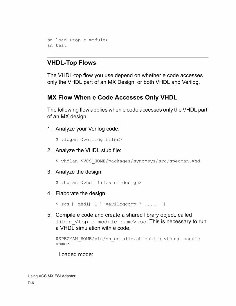
D-6
Using VCS MX ESI Adapter
sn load <top e module>sn test
VHDL-Top Flows
The VHDL-top flow you use depend on whether e code accesses only the VHDL part of an MX Design, or both VHDL and Verilog.
MX Flow When e Code Accesses Only VHDL
The following flow applies when e code accesses only the VHDL part of an MX design:
1. Analyze your Verilog code:
$ vlogan <verilog files>
2. Analyze the VHDL stub file:
$ vhdlan $VCS_HOME/packages/synopsys/src/specman.vhd
3. Analyze the design:
$ vhdlan <vhdl files of design>
4. Elaborate the design
$ scs [-mhdl] C [-verilogcomp " ..... "]
5. Compile e code and create a shared library object, called libsn_<top e module name>.so. This is necessary to run a VHDL simulation with e code.
$SPECMAN_HOME/bin/sn_compile.sh -shlib <top e module name>
Loaded mode:
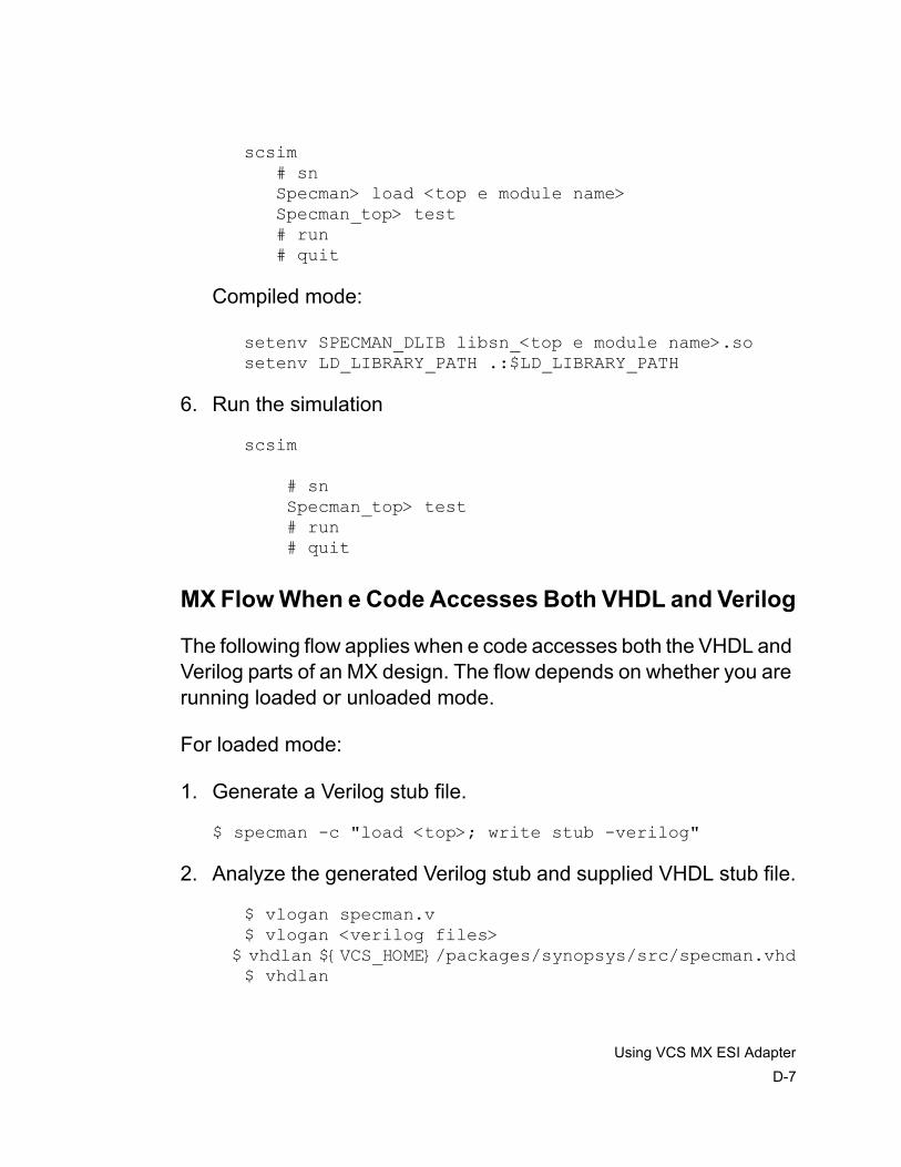
Using VCS MX ESI AdapterD-7
scsim # sn Specman> load <top e module name> Specman_top> test # run # quit
Compiled mode:
setenv SPECMAN_DLIB libsn_<top e module name>.so setenv LD_LIBRARY_PATH .:$LD_LIBRARY_PATH
6. Run the simulation
scsim
# sn Specman_top> test # run # quit
MX Flow When e Code Accesses Both VHDL and Verilog
The following flow applies when e code accesses both the VHDL and Verilog parts of an MX design. The flow depends on whether you are running loaded or unloaded mode.
For loaded mode:
1. Generate a Verilog stub file.
$ specman -c "load <top>; write stub -verilog"
2. Analyze the generated Verilog stub and supplied VHDL stub file.
$ vlogan specman.v $ vlogan <verilog files> $ vhdlan ${VCS_HOME}/packages/synopsys/src/specman.vhd $ vhdlan
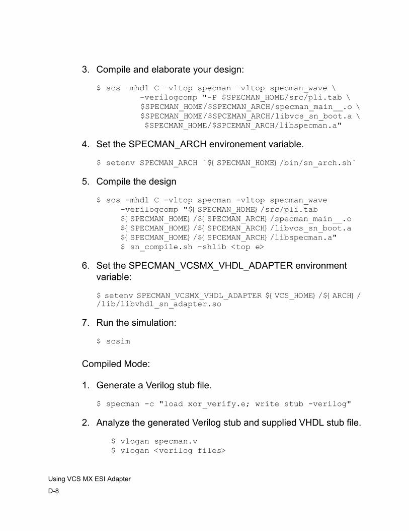
D-8
Using VCS MX ESI Adapter
3. Compile and elaborate your design:
$ scs -mhdl C -vltop specman -vltop specman_wave \ -verilogcomp "-P $SPECMAN_HOME/src/pli.tab \ $SPECMAN_HOME/$SPECMAN_ARCH/specman_main__.o \ $SPECMAN_HOME/$SPCEMAN_ARCH/libvcs_sn_boot.a \ $SPECMAN_HOME/$SPCEMAN_ARCH/libspecman.a"
4. Set the SPECMAN_ARCH environement variable.
$ setenv SPECMAN_ARCH `${SPECMAN_HOME}/bin/sn_arch.sh`
5. Compile the design
$ scs -mhdl C -vltop specman -vltop specman_wave -verilogcomp "${SPECMAN_HOME}/src/pli.tab ${SPECMAN_HOME}/${SPECMAN_ARCH}/specman_main__.o ${SPECMAN_HOME}/${SPCEMAN_ARCH}/libvcs_sn_boot.a ${SPECMAN_HOME}/${SPCEMAN_ARCH}/libspecman.a" $ sn_compile.sh -shlib <top e>
6. Set the SPECMAN_VCSMX_VHDL_ADAPTER environment variable:
$ setenv SPECMAN_VCSMX_VHDL_ADAPTER ${VCS_HOME}/${ARCH}//lib/libvhdl_sn_adapter.so
7. Run the simulation:
$ scsim
Compiled Mode:
1. Generate a Verilog stub file.
$ specman -c "load xor_verify.e; write stub -verilog"
2. Analyze the generated Verilog stub and supplied VHDL stub file.
$ vlogan specman.v $ vlogan <verilog files>
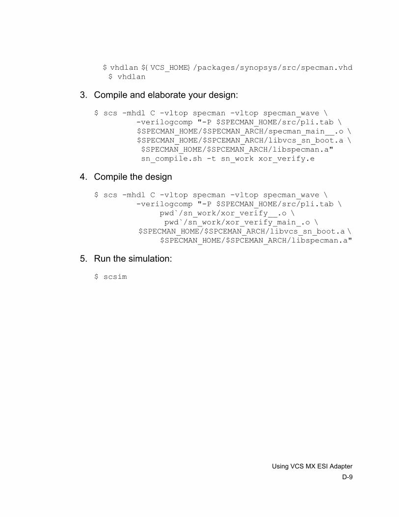
Using VCS MX ESI AdapterD-9
$ vhdlan ${VCS_HOME}/packages/synopsys/src/specman.vhd $ vhdlan
3. Compile and elaborate your design:
$ scs -mhdl C -vltop specman -vltop specman_wave \ -verilogcomp "-P $SPECMAN_HOME/src/pli.tab \ $SPECMAN_HOME/$SPECMAN_ARCH/specman_main__.o \ $SPECMAN_HOME/$SPCEMAN_ARCH/libvcs_sn_boot.a \ $SPECMAN_HOME/$SPCEMAN_ARCH/libspecman.a" sn_compile.sh -t sn_work xor_verify.e
4. Compile the design
$ scs -mhdl C -vltop specman -vltop specman_wave \ -verilogcomp "-P $SPECMAN_HOME/src/pli.tab \ pwd`/sn_work/xor_verify__.o \ pwd`/sn_work/xor_verify_main_.o \ $SPECMAN_HOME/$SPCEMAN_ARCH/libvcs_sn_boot.a \ $SPECMAN_HOME/$SPCEMAN_ARCH/libspecman.a"
5. Run the simulation:
$ scsim
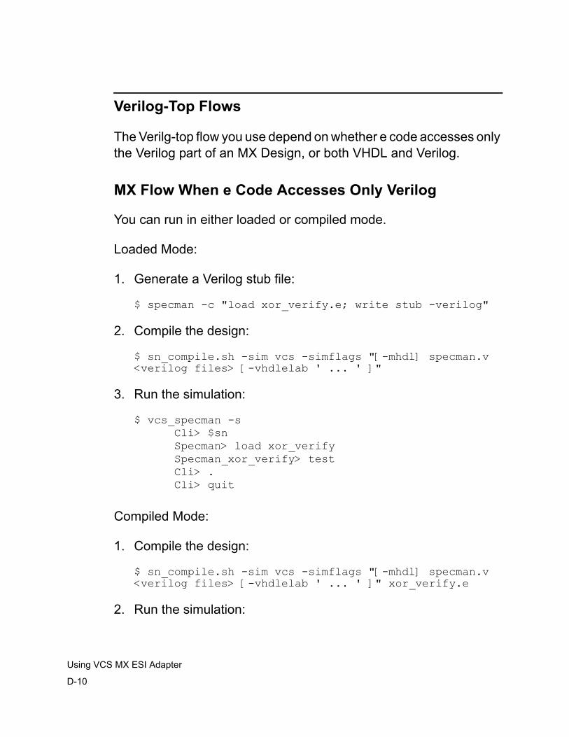
D-10
Using VCS MX ESI Adapter
Verilog-Top Flows
The Verilg-top flow you use depend on whether e code accesses only the Verilog part of an MX Design, or both VHDL and Verilog.
MX Flow When e Code Accesses Only Verilog
You can run in either loaded or compiled mode.
Loaded Mode:
1. Generate a Verilog stub file:
$ specman -c "load xor_verify.e; write stub -verilog"
2. Compile the design:
$ sn_compile.sh -sim vcs -simflags "[-mhdl] specman.v <verilog files> [-vhdlelab ' ... ' ]"
3. Run the simulation:
$ vcs_specman -s Cli> $sn Specman> load xor_verify Specman_xor_verify> test Cli> . Cli> quit
Compiled Mode:
1. Compile the design:
$ sn_compile.sh -sim vcs -simflags "[-mhdl] specman.v <verilog files> [-vhdlelab ' ... ' ]" xor_verify.e
2. Run the simulation:
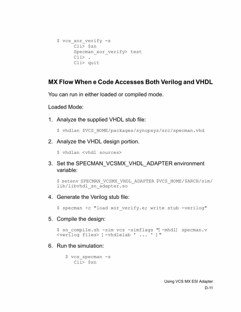
Using VCS MX ESI AdapterD-11
$ vcs_xor_verify -s Cli> $sn Specman_xor_verify> test Cli> . Cli> quit
MX Flow When e Code Accesses Both Verilog and VHDL
You can run in either loaded or compiled mode.
Loaded Mode:
1. Analyze the supplied VHDL stub file:
$ vhdlan $VCS_HOME/packages/synopsys/src/specman.vhd
2. Analyze the VHDL design portion.
$ vhdlan <vhdl sources>
3. Set the SPECMAN_VCSMX_VHDL_ADAPTER environment variable:
$ setenv SPECMAN_VCSMX_VHDL_ADAPTER $VCS_HOME/$ARCH/sim/lib/libvhdl_sn_adapter.so
4. Generate the Verilog stub file:
$ specman -c "load xor_verify.e; write stub -verilog"
5. Compile the design:
$ sn_compile.sh -sim vcs -simflags "[-mhdl] specman.v <verilog files> [-vhdlelab ' ... ' ]"
6. Run the simulation:
$ vcs_specman -s Cli> $sn
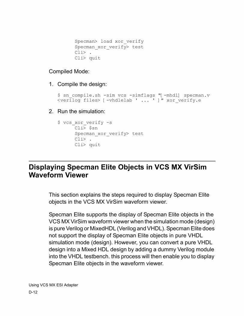
D-12
Using VCS MX ESI Adapter
Specman> load xor_verify Specman_xor_verify> test Cli> . Cli> quit
Compiled Mode:
1. Compile the design:
$ sn_compile.sh -sim vcs -simflags "[-mhdl] specman.v <verilog files> [-vhdlelab ' ... ' ]" xor_verify.e
2. Run the simulation:
$ vcs_xor_verify -s Cli> $sn Specman_xor_verify> test Cli> . Cli> quit
Displaying Specman Elite Objects in VCS MX VirSim Waveform Viewer
This section explains the steps required to display Specman Elite objects in the VCS MX VirSim waveform viewer.
Specman Elite supports the display of Specman Elite objects in the VCS MX VirSim waveform viewer when the simulation mode (design) is pure Verilog or MixedHDL (Verilog and VHDL). Specman Elite does not support the display of Specman Elite objects in pure VHDL simulation mode (design). However, you can convert a pure VHDL design into a Mixed HDL design by adding a dummy Verilog module into the VHDL testbench. this process will then enable you to display Specman Elite objects in the waveform viewer.

Using VCS MX ESI AdapterD-13
Using Specman Elite with Waveform Viewers
To display Specman Elite objects in a waveform viewer, Specman Elite creates a configuration file named wave_top-module-name.ext. This configuration file contains the definitions of all wave commands issued in the Specman Elite environment ,and is updated each time you enter a new wave command. The filename extension is determined by the waveform viewer and assigned automatically (.cfg for VirSim).
A Specman Elite configuration category, wave, has options you can specify to set up the waveform display. You use the configure wave command, or the set_config(wave, option, value) routine to set the options.
One of the wave configuration options is working_mode. Specman Elite has three working modes for waveform viewers:
• Off_line — used for batch operation, in this mode, Specman Elite only creates a top waveform configuration file, not command-specific configuration files.
• Manual — enables you to load the top waveform configuration file manually into the waveform viewer after you enter wave commands. If you enter a wave command after you load the top configuration file, you must manually load the command-specific configuration file.
• Interactive — enables you to add Specman Elite objects to the waveform viewer during the test run, using wave commands. The objects you add are traced and displayed in the viewer from that point on.
D-14
Using VCS MX ESI Adapter
Note that the VCS MX VirSim waveform viewer can be used only in off_line working mode. This is the post-processing mode for VirSim.
For a complete description of all wave configuration options, see the "Configure Wave" section in the Specman Elite Command Reference Guide of the Specman Elite distribution.
Using Specman Elite with the VirSim Waveform Viewer
To display Specman Elite objects in the VirSim viewer, you must perform several tasks in sequence. These tasks are described in the following sections:
• Setting up the VirSim Waveform Viewer
• Invoking Specman Elite with the VirSim Viewer
• Adding a Specman Elite Object to the VirSim Viewer
Setting up the VirSim Waveform Viewer
The following tasks enable you to set up the waveform viewer for Specman Elite:
• Setting waveform configuration options
• Creating the HDL stubs file
• Loading the specman_wave file
Note that setting configuration options is an optional task, but you must link Specman Elite with the VCS MX simulator, and you must create an HDL stubs file in order to enable waveform integration.
Using VCS MX ESI AdapterD-15
Setting Waveform Configuration Options for VirSimThere are several types of waveform configuration options:
• Options that affect the number of objects you can display in the waveform viewer
• Options that affect the amount of information displayed for certain types of objects
• Options that affect the way you can work with the viewer
The options that affect the number of Specman Elite objects you can display in the viewer also affect the contents of the stubs file. The stubs file contains a specman_wave module that defines a default number of registers of various typesóoutput message, error message, string, integer, boolean, and, for Verilog simulators only, event types. If you use up all the registers of a particular type, you cannot add more objects of that type to the waveform display without rewriting the stubs file.
To avoid having to rewrite and recompile the new stubs file and then re-invoke the simulation run, it makes sense to consider what additional resources your verification environment normally requires and set those configuration options in the e code using the set_config(wave) routine.
The following example shows how to set wave configuration options from e code by extending the sys.wave_setup() method:
extend sys {wave_setup() is also {set_config(wave, stub_errors, 3);};};

D-16
Using VCS MX ESI Adapter
For a complete list of all wave configuration options that affect the stubs file, see the "Using a Waveform Viewer" chapter in the Specman Elite Usage and Concepts Guide in Specman Elite distribution.
Invoking Specman Elite with the VirSim Viewer
After setting the waveform options and creating the stubs file, as described above, you are ready to compile the HDL design and invoke Specman Elite with the VCS MX simulator.
The compile procedure is demonstrated in the examples in the following sections.
You can view Specman Elite objects in the VirSim viewer after a batch run has completed.
Invoking the VirSim Viewer after a Batch RunTo invoke Specman Elite in batch mode and collect waveform data for viewing later, you should invoke specsim, rather than specview, as shown in the following example:
specsim -p "@batch.ecom;load test1;test -seed=7593;" \./vcs_cpu_top -i batch.cmd -s -f vfiles.lst >& test1.log
This example assumes that you compiled all the e code into a shared library. This example also shows two command files: batch.cmd is a simulator command file, and batch.ecom is a Specman Elite command file.
The following example shows a sample Specman Elite batch.ecom command file appropriate for batch mode:
Using VCS MX ESI AdapterD-17
1 config run -exit_on=all;2 set check ERROR;3 set wave -mode=off_line virsim4 wave exp -fields sys.cpu.next_instr5 wave exp -events -threads sys.cpu6 wave out
A description of file is as follows:
• Lines 1-2 — These commands require Specman Elite to terminate the simulation run if a DUT error or a Specman Elite error occurs.
• Line 3 — This command specifies VirSim as the viewer and the mode as batch. Specman Elite creates a single, top-level configuration file that you can manually load into the viewer at any point after the simulation run. The name of the file has the format wave_top-module.cfg. For example, if the name of the top-level e module is cpu_top, the name of the configuration file is wave_cpu_top.cfg.
• Lines 4-6 — These commands specify the Specman Elite objects that you want to display in the waveform viewer.
Generating the verilog.dump fileSince the signal data is saved in a verilog.dump file, you must execute the dumpvars system call prior to, or, at the beginning of simulation. In VCS MX, add $dumpvars to some initial block in the Verilog code.
Viewing the Waveforms in VirSim from a Batch RunTo view the waveforms from a batch run, you must load the waveform configuration file into the VirSim viewer. The viewing procedure is demonstrated in the examples in the following sections.
D-18
Using VCS MX ESI Adapter
Adding a Specman Elite Object to the VirSim Viewer
The VirSim viewer can display only one signal group at a time. To see signals from multiple groups, you can manually merge groups and then load the merged group into the viewer, or you can use several synchronized viewers at once.
Also, group names cannot be specified in Specman Elite.
To add Specman Elite objects to the waveform display, use one of the following commands, depending on the type of object you want to display:
ï wave [exp]ï wave eventï wave out
You can execute these commands from a command file or at the Specman> prompt. You can execute additional wave commands at any point during a simulation run. To review the wave commands you have executed, use the show wave command.
In off_line mode, Specman Elite creates a single configuration file that you can use at a later point to load the waveform data into viewer.
For more information on using wave command, see the "Waveform Related Commands" chapter in the Specman Elite Command Reference Guide of the Specman Elite distribution.
Using VCS MX ESI AdapterD-19
Using Specman Elite with VirSim Waveform Viewer Examples
The following two examples explain in detail the procedure to use Specman Elite to display Specman Elite objects in the VirSim waveform viewer for two Mixed HDL scenarios: one with a Verilog-top testbench, and another with a VHDL-top testbench.
The same procedure of the Mixed HDL with Verilog -op testbench applies for a pure Verilog design, but with minor modification in the HDL compile step (remove the -mhdl VCS compile option).
Mixed HDL Design with Verilog-Top Testbench Example
The example used in this section is based on the xor example distributed as part of the Specman Elite distribution. The original xor example is modified to create a scenario that shows VCS MX simulation in Mixed HDL mode with a Verilog-top testbench. The e code in this example accesses only the Verilog code of the design.
The example has the following files:
• xor_verify.e — e code that tests the xor model
• verilog_code.e — Verilog code inserted from Specman to call $dumpvars
• vl_xor.v — Verilog code that models xor behavior
• vh_xor.vhd — VHDL code that models xor behavior
• xor_tb.v — Verilog code that represents the Verilog top testbench
• synopsys_sim.setup — VCS MX setup file
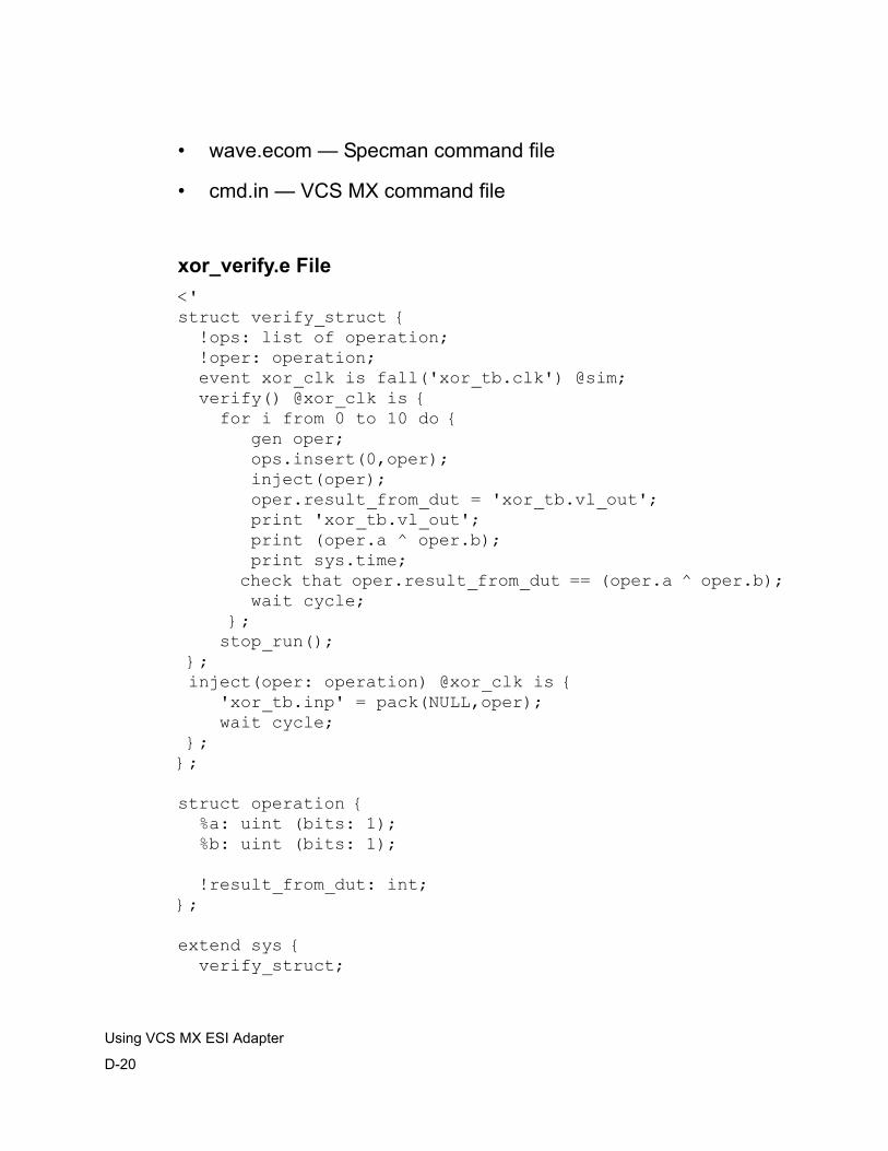
D-20
Using VCS MX ESI Adapter
• wave.ecom — Specman command file
• cmd.in — VCS MX command file
xor_verify.e File<'struct verify_struct { !ops: list of operation; !oper: operation; event xor_clk is fall('xor_tb.clk') @sim; verify() @xor_clk is { for i from 0 to 10 do { gen oper; ops.insert(0,oper); inject(oper); oper.result_from_dut = 'xor_tb.vl_out'; print 'xor_tb.vl_out'; print (oper.a ^ oper.b); print sys.time; check that oper.result_from_dut == (oper.a ̂ oper.b); wait cycle; }; stop_run(); }; inject(oper: operation) @xor_clk is { 'xor_tb.inp' = pack(NULL,oper); wait cycle; };};
struct operation { %a: uint (bits: 1); %b: uint (bits: 1);
!result_from_dut: int; };
extend sys { verify_struct;

Using VCS MX ESI AdapterD-21
run() is also { start verify_struct.verify(); };};'>
verilog_code.e<'verilog code { ""; " initial begin"; " $dumpvars;"; " end"; "";};'>
vl_xor.vmodule vl_xor (in1, in2, out1);input in1;input in2;output out1; assign out1 = in1 ^ in2;endmodule
vh_xor.vhdlibrary IEEE; use IEEE.std_logic_1164.all;
entity vh_xor is port (in1, in2: in std_logic; out1: out std_logic);end;
architecture A of vh_xor isbegin
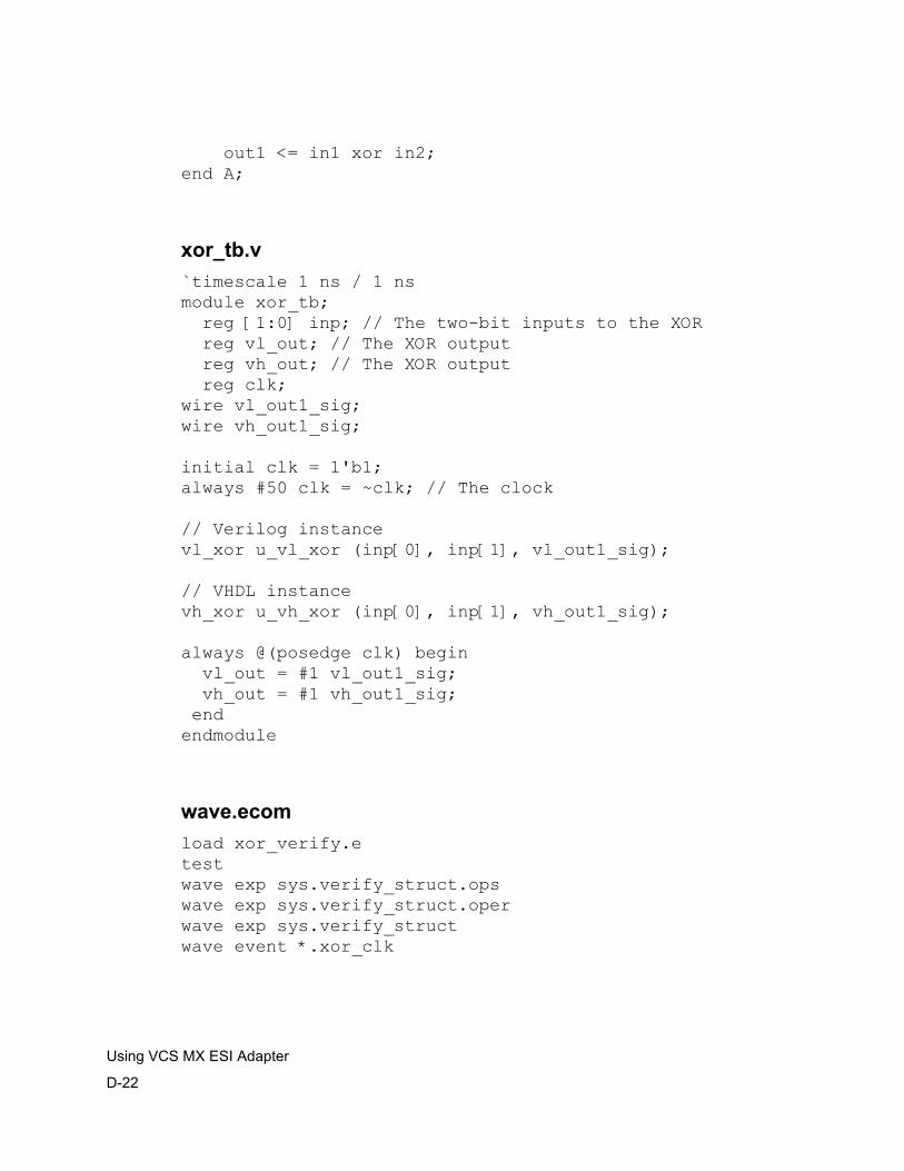
D-22
Using VCS MX ESI Adapter
out1 <= in1 xor in2;end A;
xor_tb.v`timescale 1 ns / 1 nsmodule xor_tb; reg [1:0] inp; // The two-bit inputs to the XOR reg vl_out; // The XOR output reg vh_out; // The XOR output reg clk;wire vl_out1_sig;wire vh_out1_sig;
initial clk = 1'b1;always #50 clk = ~clk; // The clock
// Verilog instancevl_xor u_vl_xor (inp[0], inp[1], vl_out1_sig);
// VHDL instancevh_xor u_vh_xor (inp[0], inp[1], vh_out1_sig);
always @(posedge clk) begin vl_out = #1 vl_out1_sig; vh_out = #1 vh_out1_sig; endendmodule
wave.ecomload xor_verify.etestwave exp sys.verify_struct.opswave exp sys.verify_struct.operwave exp sys.verify_structwave event *.xor_clk
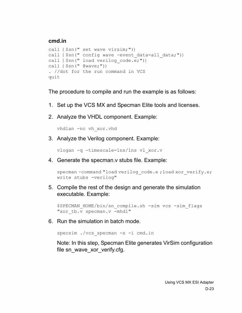
Using VCS MX ESI AdapterD-23
cmd.incall {$sn(" set wave virsim;")}call {$sn(" config wave -event_data=all_data;")}call {$sn(" load verilog_code.e;")}call {$sn(" @wave;")}. //dot for the run command in VCSquit
The procedure to compile and run the example is as follows:
1. Set up the VCS MX and Specman Elite tools and licenses.
2. Analyze the VHDL component. Example:
vhdlan -nc vh_xor.vhd
3. Analyze the Verilog component. Example:
vlogan -q -timescale=1ns/1ns vl_xor.v
4. Generate the specman.v stubs file. Example:
specman -command "load verilog_code.e ;load xor_verify.e; write stubs -verilog"
5. Compile the rest of the design and generate the simulation executable. Example:
$SPECMAN_HOME/bin/sn_compile.sh -sim vcs -sim_flags "xor_tb.v specman.v -mhdl"
6. Run the simulation in batch mode.
specsim ./vcs_specman -s -i cmd.in
Note: In this step, Specman Elite generates VirSim configuration file sn_wave_xor_verify.cfg.
D-24
Using VCS MX ESI Adapter
After the simulation is completed, do the following to see the traced Specman Elite objects in VirSim waveform viewer:
1. Invoke the VCS MX graphical user interface (VirSim) in post-processing mode.
vcs -RPP &
The hierarchy browser window will appear
2. From the hierarchy browser window, open the waveform viewer.
3. In the waveform viewer, select File > Open.
4. In the Open File dialog box, set the Type to VCD.
5. In the Open File dialog box, select the verilog.dump file.
6. Click OK in the Open File dialog box.
7. In the waveform viewer, select File > Load Configuration.
8. In the Load Configuration dialog box, turn on Incremental Load.
9. Select the top-level wave configuration file sn_wave_xor_verify.cfg and click OK.
The waveform viewer will disappear if Incremental Load was not selected. In this case, re-open the waveform viewer.
10. Select the group to be viewed (top left icon). Only one group at a time will be displayed.
The waveforms for the Specman Elite objects will appear in the waveform viewer.
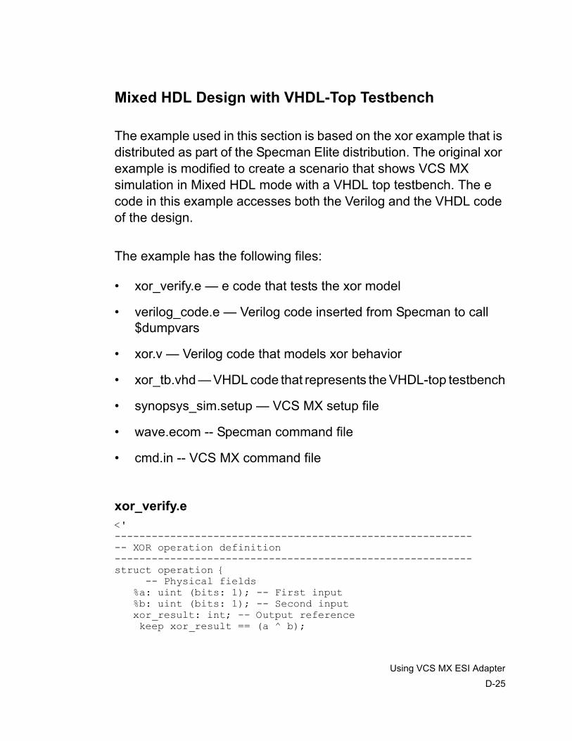
Using VCS MX ESI AdapterD-25
Mixed HDL Design with VHDL-Top Testbench
The example used in this section is based on the xor example that is distributed as part of the Specman Elite distribution. The original xor example is modified to create a scenario that shows VCS MX simulation in Mixed HDL mode with a VHDL top testbench. The e code in this example accesses both the Verilog and the VHDL code of the design.
The example has the following files:
• xor_verify.e — e code that tests the xor model
• verilog_code.e — Verilog code inserted from Specman to call $dumpvars
• xor.v — Verilog code that models xor behavior
• xor_tb.vhd — VHDL code that represents the VHDL-top testbench
• synopsys_sim.setup — VCS MX setup file
• wave.ecom -- Specman command file
• cmd.in -- VCS MX command file
xor_verify.e<'------------------------------------------------------------ XOR operation definition----------------------------------------------------------struct operation { -- Physical fields %a: uint (bits: 1); -- First input %b: uint (bits: 1); -- Second input xor_result: int; -- Output reference keep xor_result == (a ^ b);
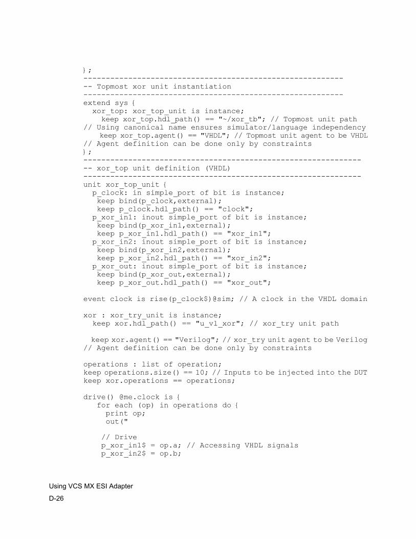
D-26
Using VCS MX ESI Adapter
};------------------------------------------------------------ Topmost xor unit instantiation----------------------------------------------------------extend sys { xor_top: xor_top_unit is instance; keep xor_top.hdl_path() == "~/xor_tb"; // Topmost unit path// Using canonical name ensures simulator/language independency keep xor_top.agent() == "VHDL"; // Topmost unit agent to be VHDL// Agent definition can be done only by constraints};---------------------------------------------------------------- xor_top unit definition (VHDL)--------------------------------------------------------------unit xor_top_unit { p_clock: in simple_port of bit is instance; keep bind(p_clock,external); keep p_clock.hdl_path() == "clock"; p_xor_in1: inout simple_port of bit is instance; keep bind(p_xor_in1,external); keep p_xor_in1.hdl_path() == "xor_in1"; p_xor_in2: inout simple_port of bit is instance; keep bind(p_xor_in2,external); keep p_xor_in2.hdl_path() == "xor_in2"; p_xor_out: inout simple_port of bit is instance; keep bind(p_xor_out,external); keep p_xor_out.hdl_path() == "xor_out";
event clock is rise(p_clock$)@sim; // A clock in the VHDL domain
xor : xor_try_unit is instance; keep xor.hdl_path() == "u_vl_xor"; // xor_try unit path
keep xor.agent() == "Verilog"; // xor_try unit agent to be Verilog// Agent definition can be done only by constraints
operations : list of operation;keep operations.size() == 10; // Inputs to be injected into the DUTkeep xor.operations == operations;
drive() @me.clock is { for each (op) in operations do { print op; out("
// Drive p_xor_in1$ = op.a; // Accessing VHDL signals p_xor_in2$ = op.b;
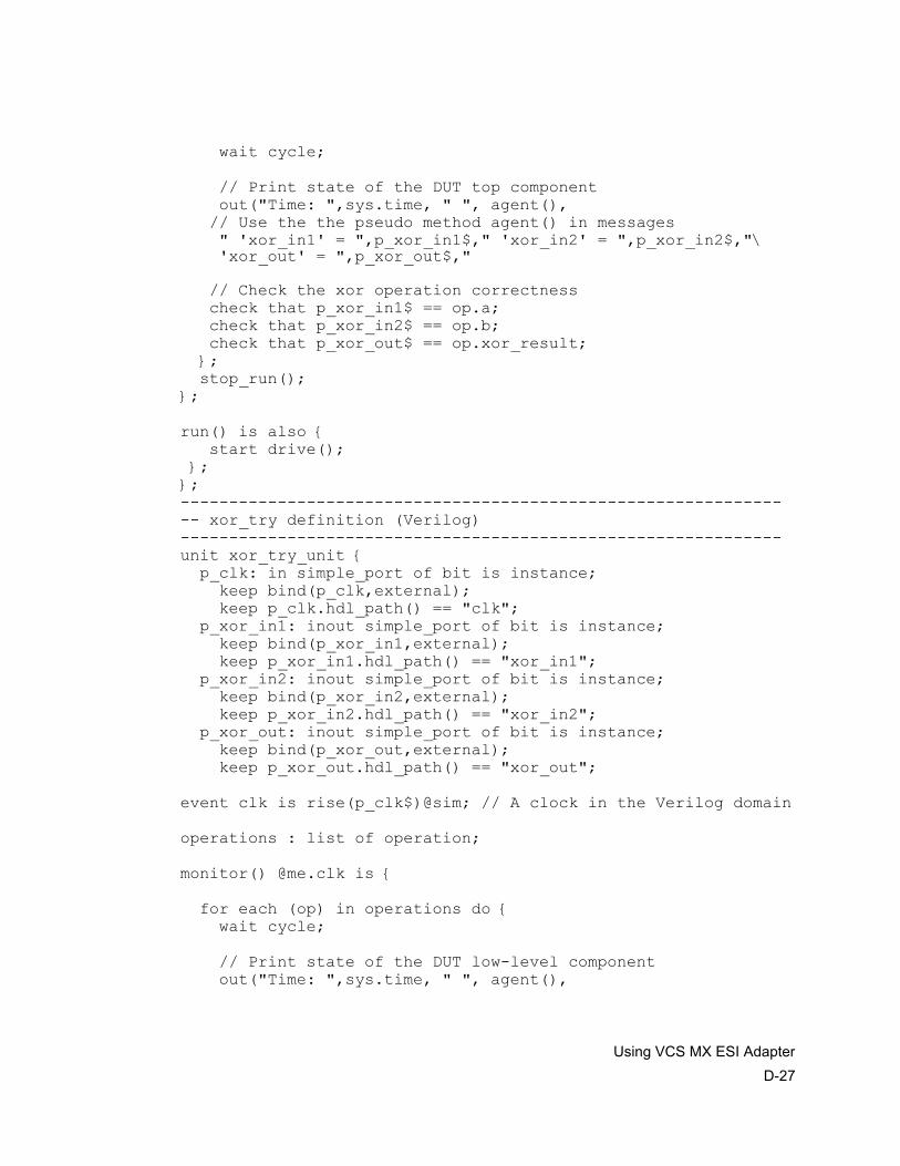
Using VCS MX ESI AdapterD-27
wait cycle;
// Print state of the DUT top component out("Time: ",sys.time, " ", agent(), // Use the the pseudo method agent() in messages " 'xor_in1' = ",p_xor_in1$," 'xor_in2' = ",p_xor_in2$,"\ 'xor_out' = ",p_xor_out$,"
// Check the xor operation correctness check that p_xor_in1$ == op.a; check that p_xor_in2$ == op.b; check that p_xor_out$ == op.xor_result; }; stop_run();};
run() is also { start drive(); };};---------------------------------------------------------------- xor_try definition (Verilog)--------------------------------------------------------------unit xor_try_unit { p_clk: in simple_port of bit is instance; keep bind(p_clk,external); keep p_clk.hdl_path() == "clk"; p_xor_in1: inout simple_port of bit is instance; keep bind(p_xor_in1,external); keep p_xor_in1.hdl_path() == "xor_in1"; p_xor_in2: inout simple_port of bit is instance; keep bind(p_xor_in2,external); keep p_xor_in2.hdl_path() == "xor_in2"; p_xor_out: inout simple_port of bit is instance; keep bind(p_xor_out,external); keep p_xor_out.hdl_path() == "xor_out";
event clk is rise(p_clk$)@sim; // A clock in the Verilog domain
operations : list of operation;
monitor() @me.clk is {
for each (op) in operations do { wait cycle;
// Print state of the DUT low-level component out("Time: ",sys.time, " ", agent(),
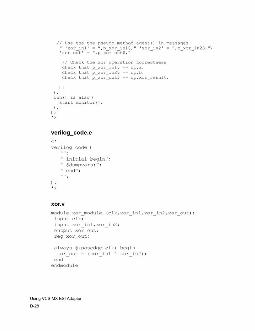
D-28
Using VCS MX ESI Adapter
// Use the the pseudo method agent() in messages " 'xor_in1' = ",p_xor_in1$," 'xor_in2' = ",p_xor_in2$,"\ 'xor_out' = ",p_xor_out$,"
// Check the xor operation correctness check that p_xor_in1$ == op.a; check that p_xor_in2$ == op.b; check that p_xor_out$ == op.xor_result;
}; }; run() is also { start monitor(); };};'>
verilog_code.e<'verilog code { ""; " initial begin"; " $dumpvars;"; " end"; "";};'>
xor.vmodule xor_module (clk,xor_in1,xor_in2,xor_out); input clk; input xor_in1,xor_in2; output xor_out; reg xor_out;
always @(posedge clk) begin xor_out = (xor_in1 ^ xor_in2); endendmodule
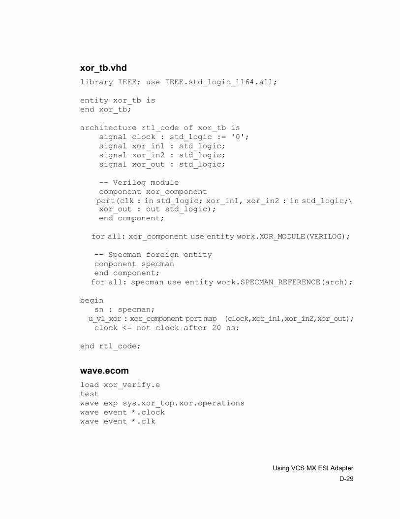
Using VCS MX ESI AdapterD-29
xor_tb.vhdlibrary IEEE; use IEEE.std_logic_1164.all;
entity xor_tb isend xor_tb;
architecture rtl_code of xor_tb is signal clock : std_logic := '0'; signal xor_in1 : std_logic; signal xor_in2 : std_logic; signal xor_out : std_logic;
-- Verilog module component xor_component port(clk : in std_logic; xor_in1, xor_in2 : in std_logic;\ xor_out : out std_logic); end component;
for all: xor_component use entity work.XOR_MODULE(VERILOG);
-- Specman foreign entity component specman end component; for all: specman use entity work.SPECMAN_REFERENCE(arch);
begin sn : specman; u_vl_xor : xor_component port map (clock,xor_in1,xor_in2,xor_out); clock <= not clock after 20 ns;
end rtl_code;
wave.ecomload xor_verify.etestwave exp sys.xor_top.xor.operationswave event *.clockwave event *.clk
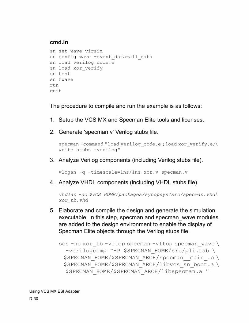
D-30
Using VCS MX ESI Adapter
cmd.insn set wave virsimsn config wave -event_data=all_datasn load verilog_code.esn load xor_verifysn testsn @waverunquit
The procedure to compile and run the example is as follows:
1. Setup the VCS MX and Specman Elite tools and licenses.
2. Generate 'specman.v' Verilog stubs file.
specman -command "load verilog_code.e ;load xor_verify.e;\ write stubs -verilog"
3. Analyze Verilog components (including Verilog stubs file).
vlogan -q -timescale=1ns/1ns xor.v specman.v
4. Analyze VHDL components (including VHDL stubs file).
vhdlan -nc $VCS_HOME/packages/synopsys/src/specman.vhd\ xor_tb.vhd
5. Elaborate and compile the design and generate the simulation executable. In this step, specman and specman_wave modules are added to the design environment to enable the display of Specman Elite objects through the Verilog stubs file.
scs -nc xor_tb -vltop specman -vltop specman_wave \ -verilogcomp "-P $SPECMAN_HOME/src/pli.tab \ $SPECMAN_HOME/$SPECMAN_ARCH/specman__main_.o \ $SPECMAN_HOME/$SPECMAN_ARCH/libvcs_sn_boot.a \ $SPECMAN_HOME/$SPECMAN_ARCH/libspecman.a "
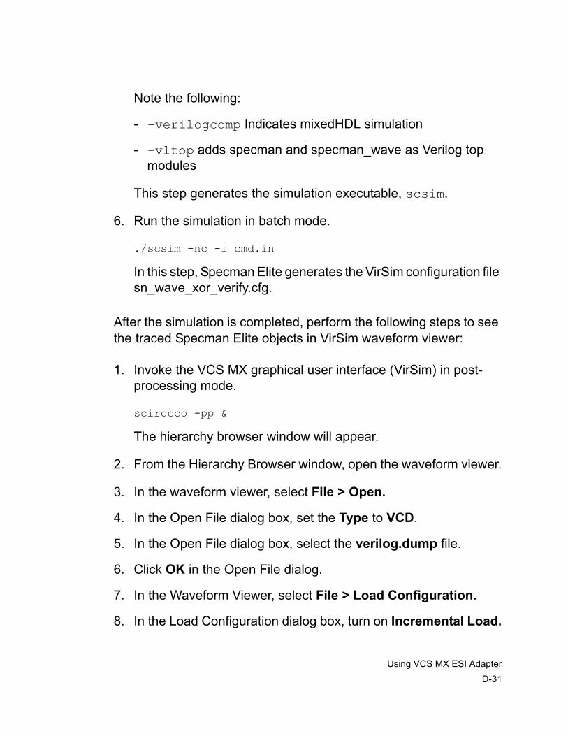
Using VCS MX ESI AdapterD-31
Note the following:
- -verilogcomp Indicates mixedHDL simulation
- -vltop adds specman and specman_wave as Verilog top modules
This step generates the simulation executable, scsim.
6. Run the simulation in batch mode.
./scsim -nc -i cmd.in
In this step, Specman Elite generates the VirSim configuration file sn_wave_xor_verify.cfg.
After the simulation is completed, perform the following steps to see the traced Specman Elite objects in VirSim waveform viewer:
1. Invoke the VCS MX graphical user interface (VirSim) in post-processing mode.
scirocco -pp &
The hierarchy browser window will appear.
2. From the Hierarchy Browser window, open the waveform viewer.
3. In the waveform viewer, select File > Open.
4. In the Open File dialog box, set the Type to VCD.
5. In the Open File dialog box, select the verilog.dump file.
6. Click OK in the Open File dialog.
7. In the Waveform Viewer, select File > Load Configuration.
8. In the Load Configuration dialog box, turn on Incremental Load.
D-32
Using VCS MX ESI Adapter
9. Select the top-level wave configuration file sn_wave_xor_verify.cfg and click OK.
The waveform viewer will disappear if Incremental Load was not selected. In this case re-open the waveform viewer.
10. Select the group to be viewed (top left icon). Only one group at a time will be displayed.
The waveforms for the Specman Elite objects will appear in the waveform viewer.
Note: The examples were verified using VCS MX version 7.1 and Specman Elite version 4.3.
E-1
Using Extended SystemVerilog Datatypes on MX Boundary
EUsing Extended SystemVerilog Datatypes on MX Boundary A
SystemVerilog supports a rich set of complex datatypes, and also allows the instantiation of ports with these new complex datatypes. This enables modules to exchange data between the complex types. VCS MX enables the exchange of the complex datatypes across the MX boundary.
The following datatypes are upported across the MX boundary layer:
• All SystemVerilog Basic 2- and 4-state Integer Types
• Enumerated Types
• Structures/Records
• Unpacked Arrays (partial support)
E2
Using Extended SystemVerilog Datatypes on MX Boundary
Integer Types
This section describes the supported SystemVerilog integer datatypes and the corresponding mapping required on the VHDL side.
The following SystemVerilog integer types are supported
• shortint : 2-state, 16 bit, signed integer
• int: 2-state, 32 bit, signed integer
• longint: 2-state, 64 bit, signed integer
• byte: 2-state, 8 bit, signed integer
• bit: 2-state, user-defined vector size
• logic: 4-state, user-defined vector size
• reg: 4-state, user-defined vector size
The following VHDL integer types are supported.
• integer: 2-state, 32 bit, signed integer
• bit and bit_vector: 2-state, user-defined vector size
• std_logic/std_ulogic/std_logic_vector/std_ulogic_vector : 9 -state, user-defined vector size
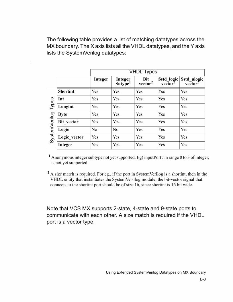
E-3
Using Extended SystemVerilog Datatypes on MX Boundary
The following table provides a list of matching datatypes across the MX boundary. The X axis lists all the VHDL datatypes, and the Y axis lists the SystemVerilog datatypes:
Note that VCS MX supports 2-state, 4-state and 9-state ports to communicate with each other. A size match is required if the VHDL port is a vector type.
.
Integer Integer Sutype1
Bit vector2
Sstd_logic vector2
Sstd_ulogic vector2
Shortint Yes Yes Yes Yes Yes
Int Yes Yes Yes Yes Yes
Longint Yes Yes Yes Yes Yes
Byte Yes Yes Yes Yes Yes
Bit_vector Yes Yes Yes Yes Yes
Logic No No Yes Yes Yes
Logic_vector Yes Yes Yes Yes Yes
Integer Yes Yes Yes Yes Yes
VHDL Types
Sys
tem
Veril
og T
ypes
1 Anonymous integer subtype not yet supported. Eg) inputPort : in range 0 to 3 of integer; is not yet supported
2 A size match is required. For eg., if the port in SystemVerilog is a shortint, then in the VHDL entity that instantiates the SystemVer-ilog module, the bit-vector signal that connects to the shortint port should be of size 16, since shortint is 16 bit wide.
E4
Using Extended SystemVerilog Datatypes on MX Boundary
Enummerated Types
SystemVerilog supports enumerated types across the ports. Three characteristics can be attributed to SystemVerilog enumerated types as given below.
• Base type of the enumerated type:
A SystemVerilog enumerated type can have a base type indicating that all the members are repre-sented using the base type.
For example:
typedef enum byte { red = 10, blue = 20, green = 30 } Colors;
In the above example, the enum's base type is byte. So all the enumerated members' (red, blue, green) value will be represented in terms of byte (8 bit integer type). However, VHDL does not have any such base type.
• User encoded values:
A SystemVerilog enumerated type can have user-defined values supplied to the enumerated mem-bers. In the example below, the member red is assigned a value 10.
For example:
typedef enum byte { red = 10, blue = 20, green = 30 } Colors;
Note that VHDL does not have any such user-defined encoding values for enumerated types.
• Number of members in the enumeration.
E-5
Using Extended SystemVerilog Datatypes on MX Boundary
This indicates what values a variable of the enumeration type can possibly take. In the example below, the enumerated type has 3 members. So a variable of type Colors can take only 3 values correspond-ing to red, blue and green.
For example:
typedef enum byte { red = 10, blue = 20, green = 30 } Colors;
Note that VCS MX supports enumerated types across the port boundary as long as they satisfy the following conditions:
- Enumerated types with user encoded values will not be supported
- Exact name match of the elements in the VHDL and SystemVerilog enumerated types is re-quired. However the enumerated type name itself need not match. In the example above the type name Colors need not match in SystemVerilog and VHDL but the members name red, blue and green should match. However, it is not case-sensitive match.
- The order of the enumerated members should be same on both SystemVerilog and VHDL.
- The number of enumerated members should be the same on both SystemVerilog and VHDL.
E6
Using Extended SystemVerilog Datatypes on MX Boundary
Structures/ Records
Structures / Records provide a useful mechanism for grouping related data together. SystemVerilog supports two kinds of structs:
• Packed — A struct whose members are all of packed types (prefixed with the packed key-word). It cannot contain fields of type unpacked arrays, real, time etc
For example:
typedef struct packed { logic [0:31] destAddress;int data;bit [0:3] parity;
} PayLoad;
• Unpacked — A struct whose members need not be of packed type.
For example:
) typedef struct { logic [0:31] destAddress; int data; bit [0:3] parity; time timestamp;
}PayLoad;
Note that the VHDL equivalent of a SystemVerilog struct is a record. VHDL does not have packed records.
The following rules apply for the exchange of SystemVerilog struct / VHDL records across the MX boundary.
E-7
Using Extended SystemVerilog Datatypes on MX Boundary
• Only SystemVerilog packed structs are supported
• Number of fields in the SystemVerilog struct and the VHDL record should be the same
• Each field of the struct should match the corresponding field of the VHDL record in size.
• The type of the field should be compatible (as indicated in the previous sections).
Arrays
SystemVerilog introduces the concept of unpacked arrays in addition to the Verilog packed arrays.
For example:
bit [3:0][7:0] joe [1:10][1:9];
The previous example defines an array of bits. The array contains 90 entries where each entry consists of 4 bytes. The dimensions [1:10][1:9] are called unpacked dimensions while [3:0][7:0] are called packed dimensions.
For supporting exchange of such arrays across VCS MX boundary, the following rules apply.
• If there is a packed dimension in SystemVerilog, the VHDL side should have a bit_vector or std_logic_vector. The length of the bit_vector or std_logic_vector in VHDL should match the combined packed dimensions in the SystemVerilog side.
E8
Using Extended SystemVerilog Datatypes on MX Boundary
• The unpacked dimensions correspond to the dimensions declared in the VHDL.
• The base type of the arrays should match.
• The number of dimensions should match.
• The size of each dimension should be the same on both sides.
• In this version of VCS MX, unpacked arrays with Verilog top is not yet supported. Only 2 levels with VHDL top is supported for multi-dimensional array ports across the VCS MX boundary.
IN-1
Index
Symbols-a filename 5-67, 7-50, 7-67-E program runtime option 7-43-grw 7-54-I 5-58-i filename 7-45-k 7-46-l filename 5-67, 7-50, 7-67-line 5-52-mhdl 5-50-Mupdate 5-51-ova_cov 7-45, 10-6-ova_cov_db 7-45-ova_cov_hier 10-6-ova_cov_name 7-45-ova_debug 10-6-ova_debug_vpd 10-6-ova_dir 10-7-ova_enable_diag 10-7-ova_file 10-7-ova_filter 7-44, 10-8-ova_filter_past 10-8-ova_inline 10-7-ova_max_fail 7-44, 10-9-ova_max_success 7-45, 10-9-ova_name 7-44-ova_quiet 7-43, 10-8
-ova_report 7-43, 10-8-ova_simend_max_fail 7-45, 10-9-ova_verbose 7-43, 10-8-PP 5-52, 5-58-q 7-50-R 5-51-RI 5-58-s 7-46-V 7-50-vcd filename 7-54-vhdlelab 5-51-vhdlrun 7-42$restart 5-63, 7-63$value$plusargs 5-66, 7-66+cliecho 7-46+maxdelays 7-55+mindelays 7-55+no_notifier 7-48+no_pulse_msg 7-51+no_tchk_msg 7-48+notimingcheck 5-67, 7-49, 7-67+override_model_delays 7-58+plus-options 7-50+sdfverbose 7-51+typdelays 7-56+v2k 3-15+vcs+dumpoff+t+ht 7-54+vcs+dumpon+t+ht 7-54
IN-2
+vcs+dumpvarsoff 5-67, 7-54, 7-67+vcs+finish 5-64, 7-49, 7-64+vcs+flush+all 7-57+vcs+flush+dump 7-57+vcs+flush+fopen 7-57+vcs+flush+log 7-57+vcs+grwavesoff 7-54+vcs+ignorestop 5-67, 7-48, 7-67+vcs+learn+pli 7-48+vcs+lic+vcsi 7-57+vcs+lic+wait 7-57+vcs+mipd+noalias 7-58+vcs+nostdout 7-51+vcs+novhdldump 7-42+vcs+stop 5-64, 7-49, 7-64+vcsi+lic+vcs 7-57+vera_load 7-46+vera_mload 7-46+vhdllib 5-51, 5-52+vpdfile 5-52
Numerics2-state code 5-114-state code 5-11
A-a filename 5-67, 7-50, 7-67acc_handle_simulated_net() PLI routine 7-58analysis
using make utility 4-11Analyzer
invoking for compiled simulationoptimizing compiled code 4-17passing options to the compiler 4-18, 5-21selecting a compiler 5-21
architecturesediting to instantiate Verilog 3-21
assertion files 10-3assertions 10-3
attributesFOREIGN
LM-family modeler 13-33
Bbackannotation
behavioral cells A-20naming conventions A-8restrictions A-18SDF files 7-8, A-1single bits A-17structural cells A-20
base time for simulation 5-27, 7-13base time unit
LM-family modeler 13-52synopsys_sim.setup 13-52
bit data type 3-22bit_vector data type 3-22boolean data type 3-22
Cchangemode
command to switch command languages 7-83
CLIspecial rules for mixed HDL simulation 7-80
+cliecho 7-46-cm 7-46-cm_dir 7-47-cm_glitch 7-47-cm_log 7-47-cm_name 7-47-cm_tglfile 7-48-cm_zip 7-48cnt.txp 10-4compiling to use interactively in mixed HDL simulation 5-58Control-c Simulator command 7-13create_smartmodel_lib command 13-5, 13-25CS_CCFLAGS_ARCH setup variable 4-19, 5-21
IN-3
CS_CCPATH_ARCH setup variable 5-21customer support -xxicycle command 5-11
example 5-14cycle elaboration reports 5-33
DData Type Mapping File
VCS/SystemC cosimulation interface 12-35data types
you can use when instantiating Verilog in VHDL 3-22
debug mode 5-18-debug option 5-11default naming convention A-8design entity
instantiating 3-12design libraries
version compatibility 4-5DEVICE SDF construct A-11DKI Communication 12-17DKI communication 12-6documentation -xviii
online -xix
E-E program 7-43editing VHDL to instantiate Verilog 3-21elaborator
Z state 5-17entity-architecture pair
LM-family modeler 13-25error messages
LM-family modeler 13-54SmartModel interface 13-18
exampletemporal assertion file 10-4
expressions 10-3
Ffacilities, test 10-3file, report 10-12files
SDF backannotation 7-8, A-1files, temporal assertion 10-3FOREIGN attribute
LM-family modeler interface 13-33
Ggcc C compiler 4-19, 5-21generic clause with LM-family modeler 13-27generic parameters
matching to SDF parameters A-8propagation A-20
genericsLMSI_DELAY_TYPE 13-29LMSI_TIMING_MEASUREMENT 13-28mapping to Verilog parameters 3-23
-grw 7-54
Hhelp -xixhotline, customer -xxiHTML report 7-7, 7-16
I-I 5-58-i filename 7-45IEEE default name mapping 1-7Ignoring Calls and License Checking 7-53Instatiating Verilog in VHDL 3-21–3-27
parameterized ports 3-25interrupting a simulation 7-13intrinsic timing delay backannotation A-11
IN-4
Jjumpered ports 3-27
K-k 7-46
L-l filename 5-67, 7-50, 7-67-latch_style option 5-12-latch_transparency option 5-12LD_LIBRARY_PATH environment variable 13-4libraries
VHDLspecifying 5-52
librarylogical name 1-6name mapping 1-6physical name 1-6
-line 5-52lm utility for LM-family modeler 13-23, 13-54LM_LIB environment variable 13-39, 13-40LMC_HOME environment variable 13-3LMC_SMARTLICENSE enviroment variable 13-4lmdaemon utility for LM-family modeler 13-23LM-family hardware modeler
architecture declaration 13-33entity declaration 13-25example 13-56FOREIGN attribute 13-33generics
LMSI_DELAY_TYPE 13-29LMSI_TIMING_MEASUREMENT 13-28
mapping pins 13-40messages
error 13-54warning 13-54
Shell Software.ADP adapter file 13-47.DEV device file 13-45
directory search order 13-39files 13-38.MDL model file 13-41.NAM name file 13-42.OPT option file 13-50.PKG package file 13-46specifying vectors in files 13-44Synopsys restrictions 13-40.TMG timing file 13-48
Simulator modeling session stepsevaluation 13-53initialization 13-52instantiation 13-36, 13-53release of resources 13-54
utilities 13-23lm utility 13-23, 13-54lmdaemon utility 13-23
VHDL model support files 13-25LMSI_DELAY_TYPE generic 13-29LMSI_TIMING_MEASUREMENT generic 13-28logical mapping 1-7
MMain Window
example 9-4overview 9-2
make utility 4-5, 4-12mapping, library name 1-6+maxdelays 7-55MemPro 1-2-mhdl 5-50+mindelays 7-55mixed event and cycle 5-9monsigs file
creating 5-18-Mupdate 5-51
Nnaming conventions
SDF timing parameters A-11
IN-5
+no_identifier 7-48+no_pulse_msg 7-51+no_tchk_msg 7-48+notimingcheck 5-67, 7-49, 7-67
Oonline documentation -xix
SOLD -xviiiOpenVera Assertions 10-1optimization levels
debug mode 5-18perf mode 5-18
output redirection 4-12simdepends command 4-9
OVAViewing Simulation Results 10-11
-ova_cov 7-45, 10-6-ova_cov_db 7-45-ova_cov_events 10-6-ova_cov_hier 10-6-ova_cov_name 7-45-ova_debug 10-6-ova_debug_vpd 10-6-ova_dir 10-7-ova_enable_diag 10-7-ova_file 10-7-ova_filter 7-44, 10-8-ova_filter_past 10-8-ova_inline 10-7-ova_max_fail 7-44, 10-9-ova_max_success 7-45, 10-9-ova_name 7-44-ova_quiet 7-43, 10-8-ova_report 7-43, 10-8-ova_simend_max_fail 7-45, 10-9-ova_success 7-45, 10-9-ova_verbose 7-43, 10-8+override_model_delays 7-58
Ppartition file
creating 5-9syntax 5-11VHDL
differentiating event-driven and cycle-based 5-54
perf mode 5-18-perf option 5-11physical mapping 1-7+plus-options 7-50Port Mapping File
VCS/SystemC cosimulation interface 12-32ports
jumpered 3-27-PP 5-52, 5-58PROPAGATE_VALUE VHDL attribute A-20propagation of generic parameters A-21
Q-q 7-50quit Simulator command 7-15quitting
Simulator 7-15
R-R 5-51reanalyzing source files 4-11report file 10-12$restart 5-63, 7-63restart Simulator command 7-14restarting a simulation 7-14results 10-12-RI 5-58run Simulator command
executing 7-13running a simulation 7-13
IN-6
S-s 7-46SDF backannotation
header file A-7ignored constructs A-19restrictions A-18single bits A-17
sdf_header.vhd package file A-7sdf_naming.s file A-10SDFNAMINGFILE setup variable A-10SDFPOLICY setup variable A-15+sdfverbose 7-51SDFWILDCARD setup variable A-6setup file 13-82setup files
synopsys_sim.setup 1-4setup variables
TIMEBASELM-family modeler 13-52
Shell Software.ADP adapter file 13-47.DEV device file 13-45directory search order 13-39files 13-38.MDL model file 13-41.NAM name file 13-42.OPT option file 13-50.PKG package file 13-46specifying vectors in files 13-44Synopsys restrictions 13-40.TMG timing file 13-48
simcompiled utility 4-12simdepends utility 4-5simulation
hardware models 1-2mixed event and cycle 5-6, 5-9
Simulatorinterrupting 7-13restarting 7-14running 7-13
simulator graphical user interface 7-3single bit backannotation A-17
SmartModelscomponents, instantiation 13-12environment setup 13-3error messages 13-18library clause 13-12port and window names 13-10use clause 13-12user-defined timing files 13-19warning messages 13-18windows 13-13
SolvNet -xixstd_logic data type 3-22std_logic_vector data type 3-22std_ulogic data type 3-22std_ulogic_vector data type 3-22structural cell back-annotation A-20summary report 5-34support, customer -xxiSynopsys setup file .synopsys_vss.setup
SmartModel requirements 13-10, 13-11TIMEBASE variable
LM-family modeler 13-52Synopsys web page -xxSYNOPSYS_SIM
default name mapping 1-7-sysc 12-14syscan utility 12-8–12-11SystemC
cosimulating with Verilog 12-1SYSTEMC_OVERRIDE environment variable 12-39
T-t option
vhdlsimLM-family modeler 13-52
technical support -xxiTelecom workbench 1-2temporal assertion files 10-3temporal assertions 10-3temporal expressions 10-3test facilities 10-3
IN-7
TIMEBASE setup variableLM-family modeler 13-52overriding 7-13
timebase variable 5-27top-level generics 5-22trigger report 5-38triggers, types of 5-45+typdelays 7-56
UUCLI 7-12unconnected ports 3-27
V-V 7-50+v2k 3-15$value$plusargs 5-66, 7-66-vcd filename 7-54VCD+
Command line optionsIgnore $vcdplus calls in code 7-53
+vcs+dumpoff+t+ht 7-54+vcs+dumpon+t+ht 7-54+vcs+dumpvarsoff 5-67, 7-54, 7-67+vcs+finish 5-64, 7-49, 7-64+vcs+flush+all 7-57+vcs+flush+dump 7-57+vcs+flush+fopen 7-57+vcs+flush+log 7-57+vcs+grwavesoff 7-54+vcs+ignorestop 5-67, 7-48, 7-67+vcs+learn+pli 7-48+vcs+lic+vcsi 7-57+vcs+lic+wait 7-57+vcs+mipd+noalias 7-58+vcs+nostdout 7-51+vcs+novhdldump 7-42+vcs+stop 5-64, 7-49, 7-64
VCS/SystemC cosimulation interface 12-1–12-40
compiling for using 12-14, 12-24supported port data types 12-8
+vcsi+lic+vcs 7-57+vera_load 7-46+vera_mload 7-46verify 10-12VHDL
circumventing rules for identifiers 3-27data types
you can use when instantiating Verilog 3-22
extended identifiers 3-27generics
mapping to Verilog parameters 3-23instantiating top-level design entity 3-12
binding the instance to a design unit 3-20connecting Verilog signals to VHDL ports
3-16instantiating by configuration name 3-14instantiating by entity name 3-13passing parameter values to generics 3-15with a variable port width 3-17
librariesspecifying 5-52
partition filedifferentiating event-driven and cycle-
based 5-54VHDL Analyzer
invoking with vhdlan 2-8vhdlan command
syntax 2-8-vhdlelab 5-51+vhdllib 5-51, 5-52-vhdlrun 7-42VhMC models 1-2VirSim 5-58
restarting for scsim options 7-78virsim
syntax 7-40VITAL models
error messages B-5VITAL netlist B-7
IN-8
backannotation B-8negative constraints calculation B-11
vlogan utility 12-18–12-20VMC 7-77+vpdfile 5-52
Wwarning messages
LM-family modeler 13-54SmartModel interface 13-18
Waveform Windowoverview 9-8, 9-9
web page, Synopsys -xxwildcards
SDF file A-6windows 13-13World Wide Web page, Synopsys -xxwrapper for VCS/SystemC cosimulation
instantiating in SystemC 12-22SystemC in Verilog 12-8Verilog in SystemC 12-18
ZZ state 5-17