Embed Size (px)
Citation preview
VEC Tutorial
Dean Fantazzini
Dipartimento di Economia Politica e Metodi Quantitativi
University of Pavia
Overview of the Lecture
1st A review of Johansen’s approach for cointegration
Advanced Time Series Econometrics
Dean Fantazzini 10 − 15 July 2006 2
Overview of the Lecture
1st A review of Johansen’s approach for cointegration
2nd An empirical example: the long run Phillips curve
Advanced Time Series Econometrics
Dean Fantazzini 10 − 15 July 2006 2-a
Overview of the Lecture
1st A review of Johansen’s approach for cointegration
2nd An empirical example: the long run Phillips curve
3rd An empirical example: Italian Treasury bills interest rates
Advanced Time Series Econometrics
Dean Fantazzini 10 − 15 July 2006 2-b
Overview of the Lecture
1st A review of Johansen’s approach for cointegration
2nd An empirical example: the long run Phillips curve
3rd An empirical example: Italian Treasury bills interest rates
4th An empirical example: A model for the Danish Economy
Advanced Time Series Econometrics
Dean Fantazzini 10 − 15 July 2006 2-c
A review of Johansen’s approach for cointegration
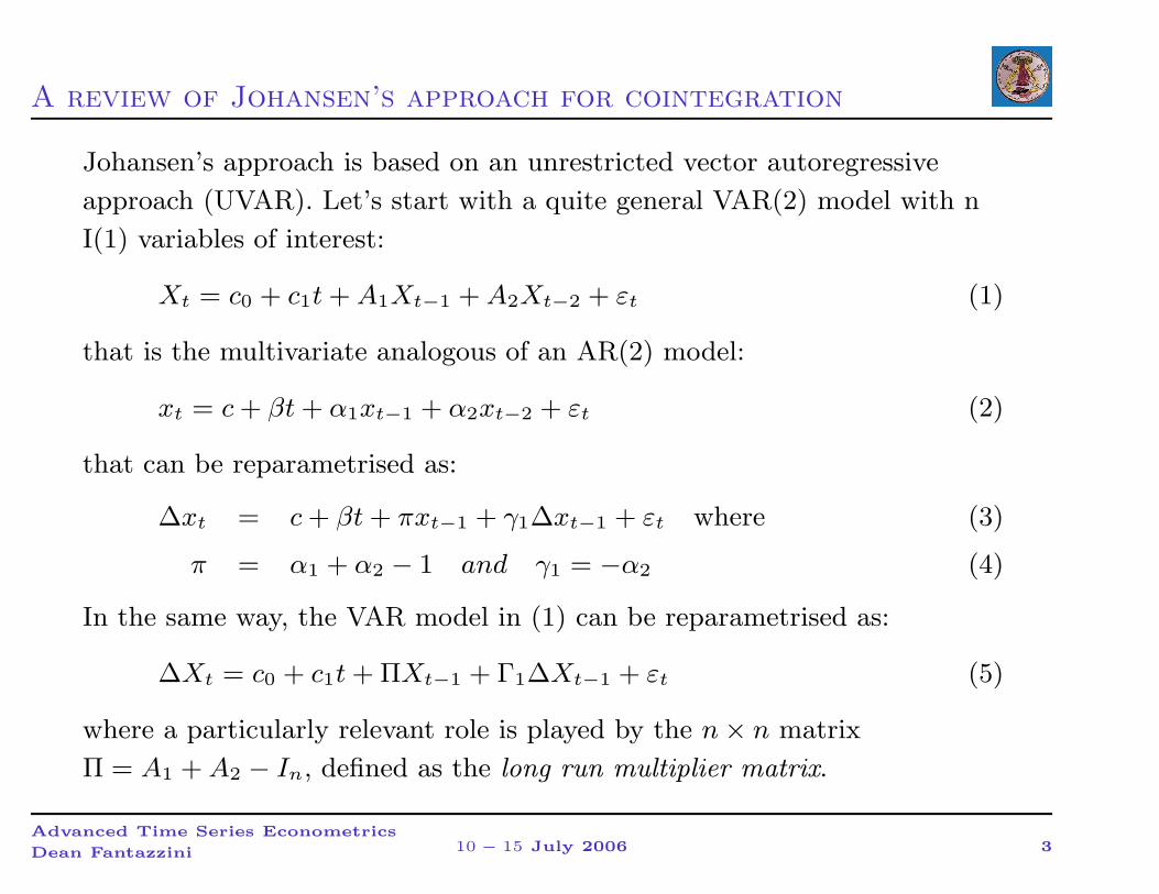
Johansen’s approach is based on an unrestricted vector autoregressive
approach (UVAR). Let’s start with a quite general VAR(2) model with n
I(1) variables of interest:
Xt = c0 + c1t + A1Xt−1 + A2Xt−2 + εt (1)
that is the multivariate analogous of an AR(2) model:
xt = c + βt + α1xt−1 + α2xt−2 + εt (2)
that can be reparametrised as:
∆xt = c + βt + πxt−1 + γ1∆xt−1 + εt where (3)
π = α1 + α2 − 1 and γ1 = −α2 (4)
In the same way, the VAR model in (1) can be reparametrised as:
∆Xt = c0 + c1t + ΠXt−1 + Γ1∆Xt−1 + εt (5)
where a particularly relevant role is played by the n × n matrix
Π = A1 + A2 − In, defined as the long run multiplier matrix.
Advanced Time Series Econometrics
Dean Fantazzini 10 − 15 July 2006 3
A review of Johansen’s approach for cointegration
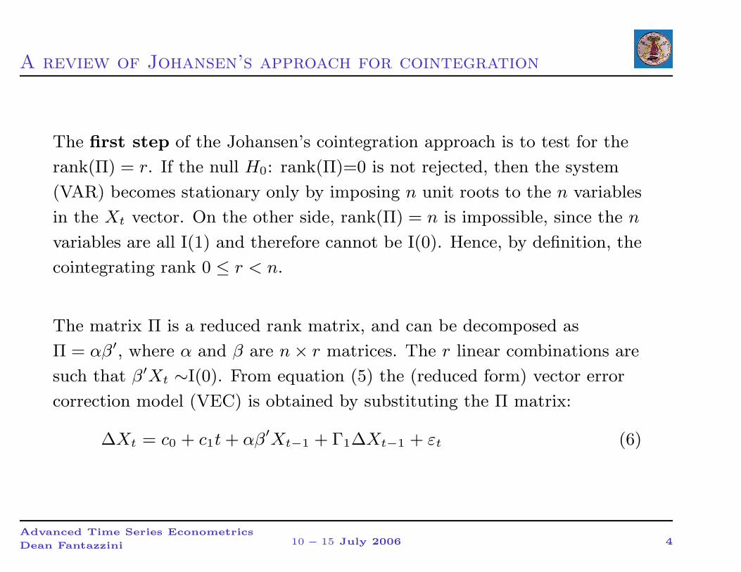
The first step of the Johansen’s cointegration approach is to test for the
rank(Π) = r. If the null H0: rank(Π)=0 is not rejected, then the system
(VAR) becomes stationary only by imposing n unit roots to the n variables
in the Xt vector. On the other side, rank(Π) = n is impossible, since the n
variables are all I(1) and therefore cannot be I(0). Hence, by definition, the
cointegrating rank 0 ≤ r < n.
The matrix Π is a reduced rank matrix, and can be decomposed as
Π = αβ′, where α and β are n × r matrices. The r linear combinations are
such that β′Xt ∼I(0). From equation (5) the (reduced form) vector error
correction model (VEC) is obtained by substituting the Π matrix:
∆Xt = c0 + c1t + αβ′
Xt−1 + Γ1∆Xt−1 + εt (6)
Advanced Time Series Econometrics
Dean Fantazzini 10 − 15 July 2006 4
A review of Johansen’s approach for cointegration
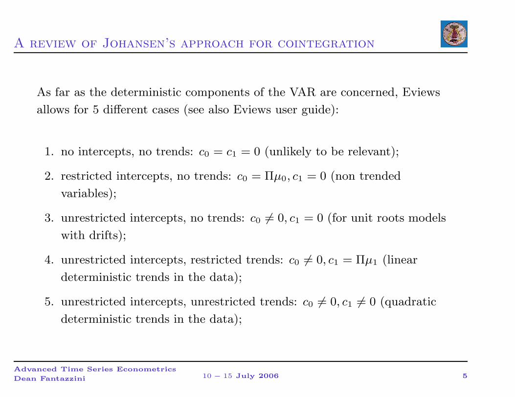
As far as the deterministic components of the VAR are concerned, Eviews
allows for 5 different cases (see also Eviews user guide):
1. no intercepts, no trends: c0 = c1 = 0 (unlikely to be relevant);
2. restricted intercepts, no trends: c0 = Πµ0, c1 = 0 (non trended
variables);
3. unrestricted intercepts, no trends: c0 6= 0, c1 = 0 (for unit roots models
with drifts);
4. unrestricted intercepts, restricted trends: c0 6= 0, c1 = Πµ1 (linear
deterministic trends in the data);
5. unrestricted intercepts, unrestricted trends: c0 6= 0, c1 6= 0 (quadratic
deterministic trends in the data);
Advanced Time Series Econometrics
Dean Fantazzini 10 − 15 July 2006 5
A review of Johansen’s approach for cointegration
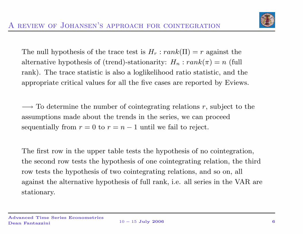
The null hypothesis of the trace test is Hr : rank(Π) = r against the
alternative hypothesis of (trend)-stationarity: Hn : rank(π) = n (full
rank). The trace statistic is also a loglikelihood ratio statistic, and the
appropriate critical values for all the five cases are reported by Eviews.
−→ To determine the number of cointegrating relations r, subject to the
assumptions made about the trends in the series, we can proceed
sequentially from r = 0 to r = n − 1 until we fail to reject.
The first row in the upper table tests the hypothesis of no cointegration,
the second row tests the hypothesis of one cointegrating relation, the third
row tests the hypothesis of two cointegrating relations, and so on, all
against the alternative hypothesis of full rank, i.e. all series in the VAR are
stationary.
Advanced Time Series Econometrics
Dean Fantazzini 10 − 15 July 2006 6
A review of Johansen’s approach for cointegration
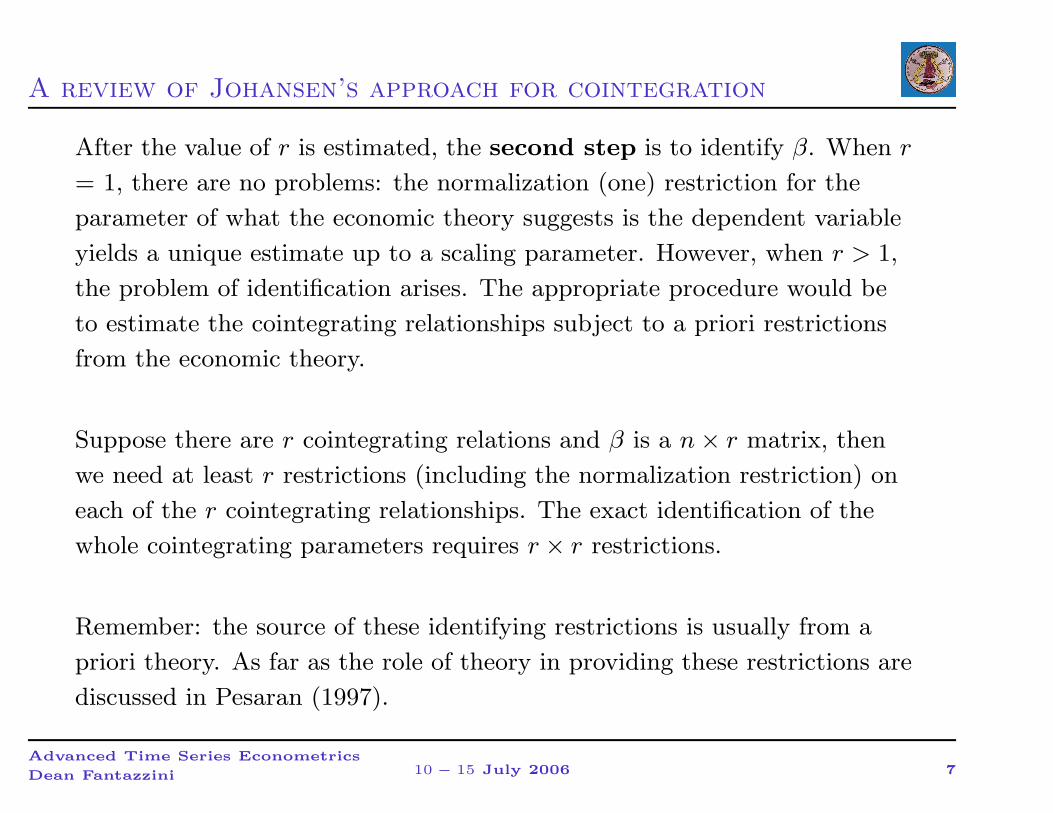
After the value of r is estimated, the second step is to identify β. When r
= 1, there are no problems: the normalization (one) restriction for the
parameter of what the economic theory suggests is the dependent variable
yields a unique estimate up to a scaling parameter. However, when r > 1,
the problem of identification arises. The appropriate procedure would be
to estimate the cointegrating relationships subject to a priori restrictions
from the economic theory.
Suppose there are r cointegrating relations and β is a n × r matrix, then
we need at least r restrictions (including the normalization restriction) on
each of the r cointegrating relationships. The exact identification of the
whole cointegrating parameters requires r × r restrictions.
Remember: the source of these identifying restrictions is usually from a
priori theory. As far as the role of theory in providing these restrictions are
discussed in Pesaran (1997).
Advanced Time Series Econometrics
Dean Fantazzini 10 − 15 July 2006 7
An empirical example: the long run Phillips curve
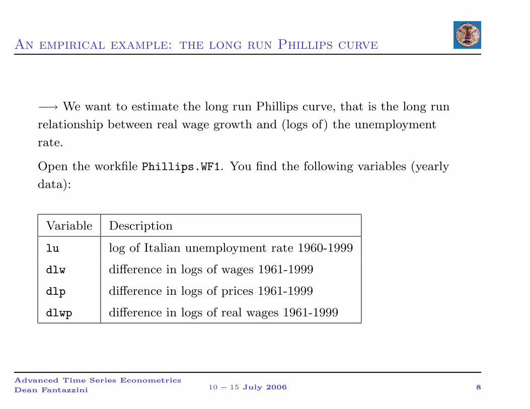
−→ We want to estimate the long run Phillips curve, that is the long run
relationship between real wage growth and (logs of) the unemployment
rate.
Open the workfile Phillips.WF1. You find the following variables (yearly
data):
Variable Description
lu log of Italian unemployment rate 1960-1999
dlw difference in logs of wages 1961-1999
dlp difference in logs of prices 1961-1999
dlwp difference in logs of real wages 1961-1999
Advanced Time Series Econometrics
Dean Fantazzini 10 − 15 July 2006 8
An empirical example: the long run Phillips curve
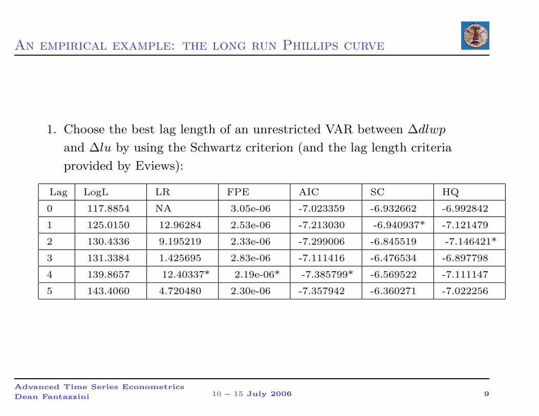
1. Choose the best lag length of an unrestricted VAR between ∆dlwp
and ∆lu by using the Schwartz criterion (and the lag length criteria
provided by Eviews):
Lag LogL LR FPE AIC SC HQ
0 117.8854 NA 3.05e-06 -7.023359 -6.932662 -6.992842
1 125.0150 12.96284 2.53e-06 -7.213030 -6.940937* -7.121479
2 130.4336 9.195219 2.33e-06 -7.299006 -6.845519 -7.146421*
3 131.3384 1.425695 2.83e-06 -7.111416 -6.476534 -6.897798
4 139.8657 12.40337* 2.19e-06* -7.385799* -6.569522 -7.111147
5 143.4060 4.720480 2.30e-06 -7.357942 -6.360271 -7.022256
Advanced Time Series Econometrics
Dean Fantazzini 10 − 15 July 2006 9
An empirical example: the long run Phillips curve
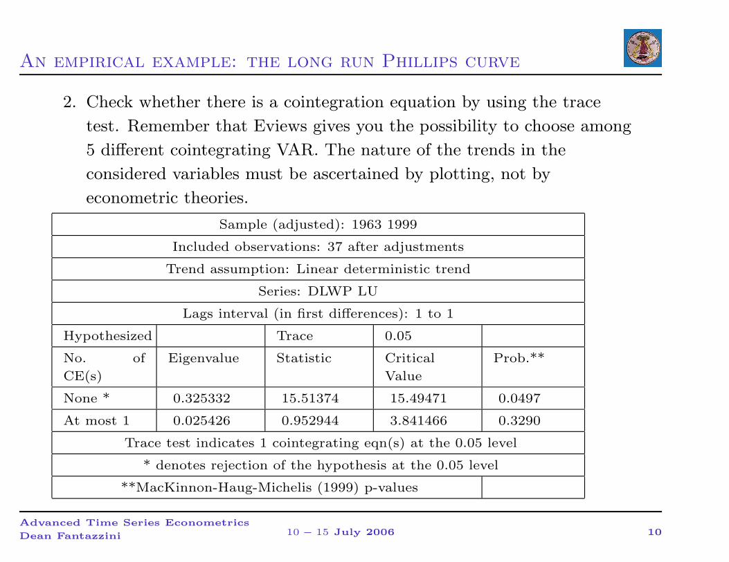
2. Check whether there is a cointegration equation by using the trace
test. Remember that Eviews gives you the possibility to choose among
5 different cointegrating VAR. The nature of the trends in the
considered variables must be ascertained by plotting, not by
econometric theories.
Sample (adjusted): 1963 1999
Included observations: 37 after adjustments
Trend assumption: Linear deterministic trend
Series: DLWP LU
Lags interval (in first differences): 1 to 1
Hypothesized Trace 0.05
No. of
CE(s)
Eigenvalue Statistic Critical
Value
Prob.**
None * 0.325332 15.51374 15.49471 0.0497
At most 1 0.025426 0.952944 3.841466 0.3290
Trace test indicates 1 cointegrating eqn(s) at the 0.05 level
* denotes rejection of the hypothesis at the 0.05 level
**MacKinnon-Haug-Michelis (1999) p-values
Advanced Time Series Econometrics
Dean Fantazzini 10 − 15 July 2006 10
An empirical example: the long run Phillips curve
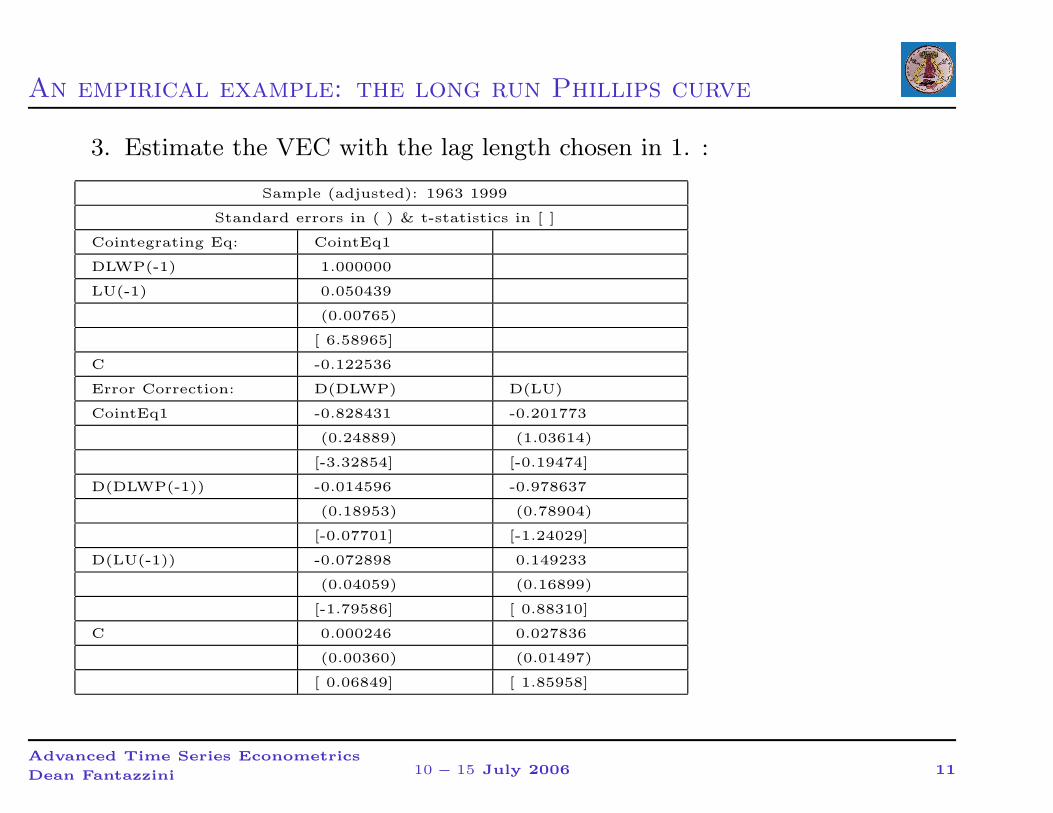
3. Estimate the VEC with the lag length chosen in 1. :
Sample (adjusted): 1963 1999
Standard errors in ( ) & t-statistics in [ ]
Cointegrating Eq: CointEq1
DLWP(-1) 1.000000
LU(-1) 0.050439
(0.00765)
[ 6.58965]
C -0.122536
Error Correction: D(DLWP) D(LU)
CointEq1 -0.828431 -0.201773
(0.24889) (1.03614)
[-3.32854] [-0.19474]
D(DLWP(-1)) -0.014596 -0.978637
(0.18953) (0.78904)
[-0.07701] [-1.24029]
D(LU(-1)) -0.072898 0.149233
(0.04059) (0.16899)
[-1.79586] [ 0.88310]
C 0.000246 0.027836
(0.00360) (0.01497)
[ 0.06849] [ 1.85958]
Advanced Time Series Econometrics
Dean Fantazzini 10 − 15 July 2006 11
An empirical example: the long run Phillips curve
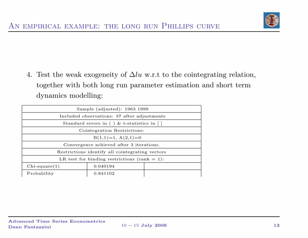
4. Test the weak exogeneity of ∆lu w.r.t to the cointegrating relation,
together with both long run parameter estimation and short term
dynamics modelling:
Sample (adjusted): 1963 1999
Included observations: 37 after adjustments
Standard errors in ( ) & t-statistics in [ ]
Cointegration Restrictions:
B(1,1)=1, A(2,1)=0
Convergence achieved after 3 iterations.
Restrictions identify all cointegrating vectors
LR test for binding restrictions (rank = 1):
Chi-square(1) 0.040194
Probability 0.841102
Advanced Time Series Econometrics
Dean Fantazzini 10 − 15 July 2006 12
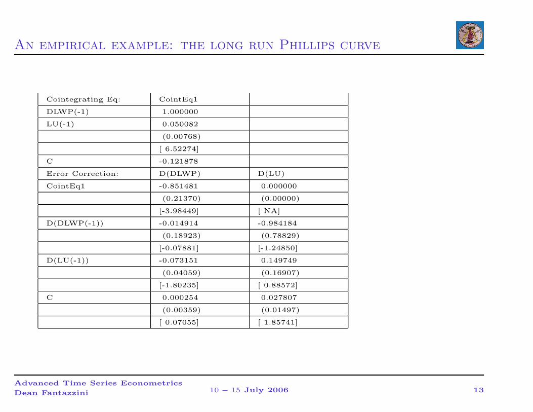
An empirical example: the long run Phillips curve
Cointegrating Eq: CointEq1
DLWP(-1) 1.000000
LU(-1) 0.050082
(0.00768)
[ 6.52274]
C -0.121878
Error Correction: D(DLWP) D(LU)
CointEq1 -0.851481 0.000000
(0.21370) (0.00000)
[-3.98449] [ NA]
D(DLWP(-1)) -0.014914 -0.984184
(0.18923) (0.78829)
[-0.07881] [-1.24850]
D(LU(-1)) -0.073151 0.149749
(0.04059) (0.16907)
[-1.80235] [ 0.88572]
C 0.000254 0.027807
(0.00359) (0.01497)
[ 0.07055] [ 1.85741]
Advanced Time Series Econometrics
Dean Fantazzini 10 − 15 July 2006 13
An empirical example: the long run Phillips curve
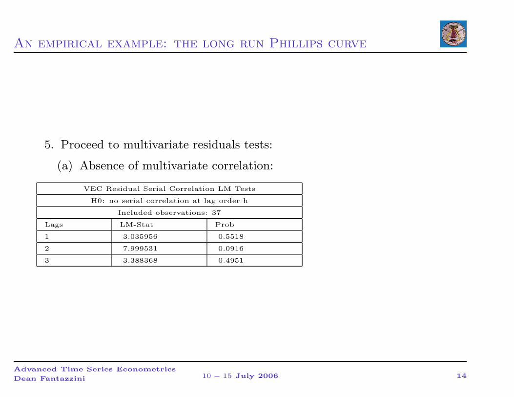
5. Proceed to multivariate residuals tests:
(a) Absence of multivariate correlation:
VEC Residual Serial Correlation LM Tests
H0: no serial correlation at lag order h
Included observations: 37
Lags LM-Stat Prob
1 3.035956 0.5518
2 7.999531 0.0916
3 3.388368 0.4951
Advanced Time Series Econometrics
Dean Fantazzini 10 − 15 July 2006 14
An empirical example: the long run Phillips curve
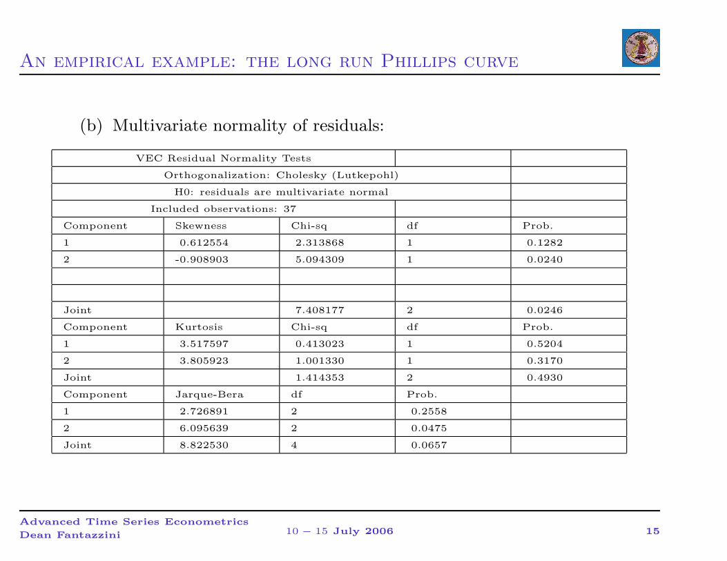
(b) Multivariate normality of residuals:
VEC Residual Normality Tests
Orthogonalization: Cholesky (Lutkepohl)
H0: residuals are multivariate normal
Included observations: 37
Component Skewness Chi-sq df Prob.
1 0.612554 2.313868 1 0.1282
2 -0.908903 5.094309 1 0.0240
Joint 7.408177 2 0.0246
Component Kurtosis Chi-sq df Prob.
1 3.517597 0.413023 1 0.5204
2 3.805923 1.001330 1 0.3170
Joint 1.414353 2 0.4930
Component Jarque-Bera df Prob.
1 2.726891 2 0.2558
2 6.095639 2 0.0475
Joint 8.822530 4 0.0657
Advanced Time Series Econometrics
Dean Fantazzini 10 − 15 July 2006 15
An empirical example: the long run Phillips curve
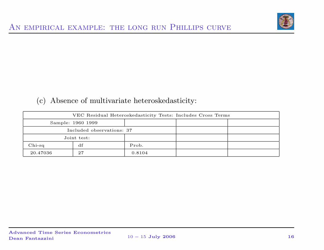
(c) Absence of multivariate heteroskedasticity:
VEC Residual Heteroskedasticity Tests: Includes Cross Terms
Sample: 1960 1999
Included observations: 37
Joint test:
Chi-sq df Prob.
20.47036 27 0.8104
Advanced Time Series Econometrics
Dean Fantazzini 10 − 15 July 2006 16
An empirical example: Italian Treasury bills interest rates
−→ Another example can be drawn from Italian Treasury bills interest
rates.
Open the file termine.wf1. We have 3, 6, 12 month bills. Repeat all the
steps you did with the Phillips curve example, remembering that there
should be 2 cointegration relationships: 1) Between the 3 and 12 months
Treasury bills; 2) Between the 6 and 12 months Treasury bills.
The 12 months Treasury bill should be weak exogenous.
Advanced Time Series Econometrics
Dean Fantazzini 10 − 15 July 2006 17
An empirical example: A model for the Danish Economy
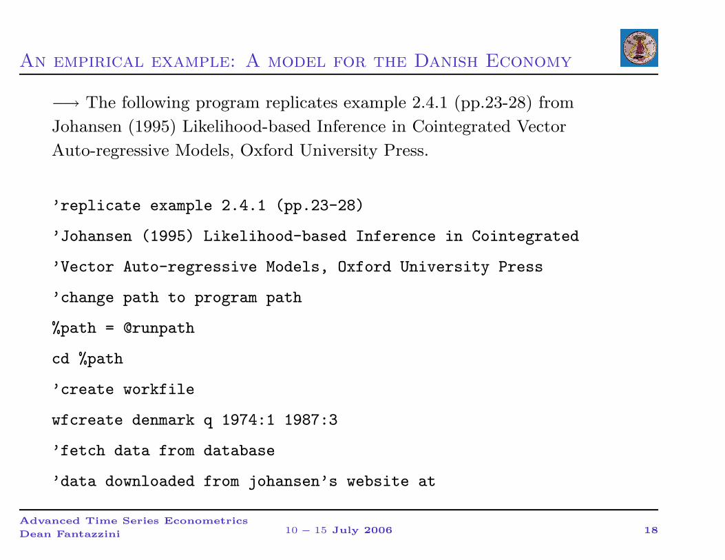
−→ The following program replicates example 2.4.1 (pp.23-28) from
Johansen (1995) Likelihood-based Inference in Cointegrated Vector
Auto-regressive Models, Oxford University Press.
’replicate example 2.4.1 (pp.23-28)
’Johansen (1995) Likelihood-based Inference in Cointegrated
’Vector Auto-regressive Models, Oxford University Press
’change path to program path
%path = @runpath
cd %path
’create workfile
wfcreate denmark q 1974:1 1987:3
’fetch data from database
’data downloaded from johansen’s website at
Advanced Time Series Econometrics
Dean Fantazzini 10 − 15 July 2006 18
An empirical example: A model for the Danish Economy
’http://www.math.ku.dk/ sjo/data/data.html
fetch(d=var dat) lrm lry ibo ide
’create centered seasonal dummies
for !i=1 to 3
series d!i = @seas(!i) - 0.25
next
’estimate unrestricted VAR
var var1.ls 1 2 lrm lry ibo ide @ c d1 d2 d3
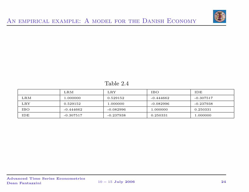
’replicate residual correlation matrix Table 2.4 (p.24)
freeze(tab24) var1.residcor
show tab24
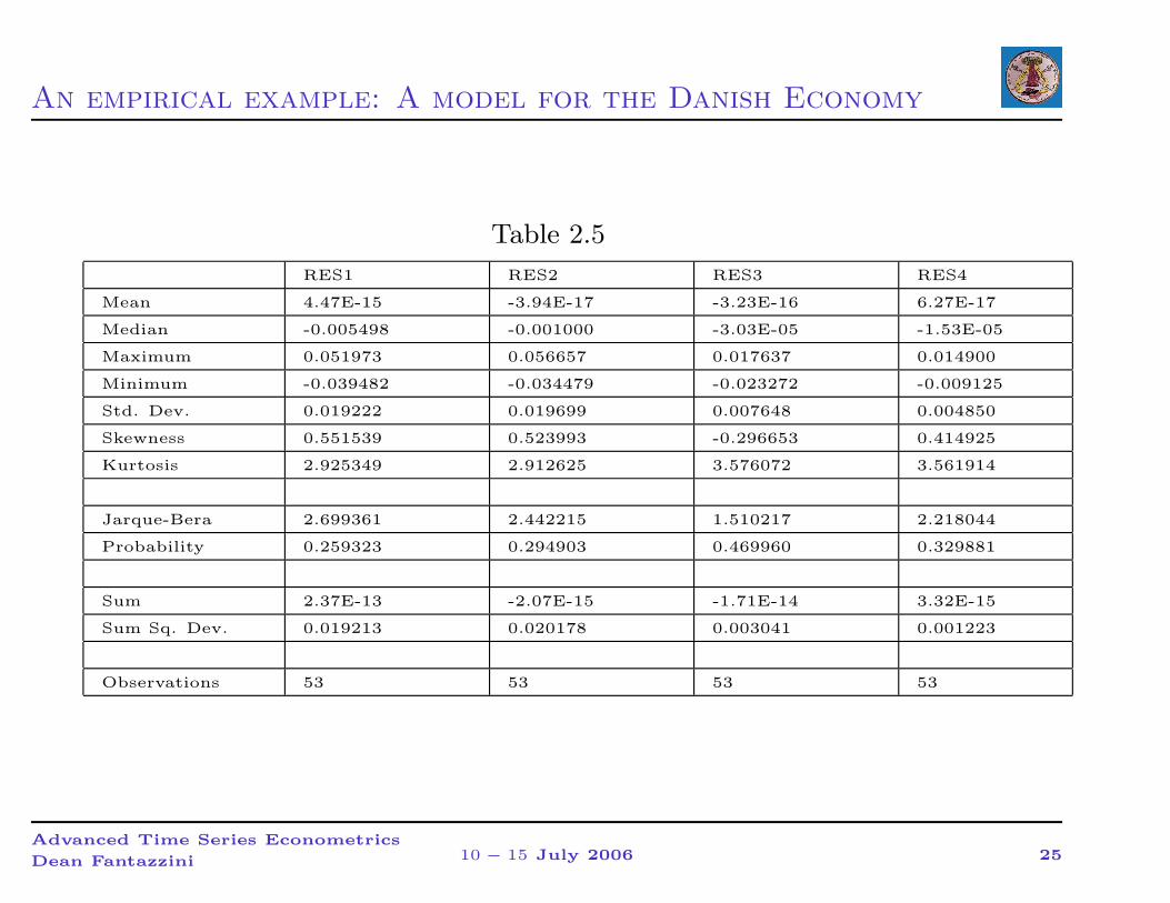
’replicate univariate residual diagnostics Table 2.5 (p.25)
’note that Johansen reports *excess* kurtosis relative to 3.0
Advanced Time Series Econometrics
Dean Fantazzini 10 − 15 July 2006 19
An empirical example: A model for the Danish Economy
’also JB statistic does not match; why?
var1.makeresid(name=gres) res1 res2 res3 res4
freeze(tab25) gres.stats
show tab25
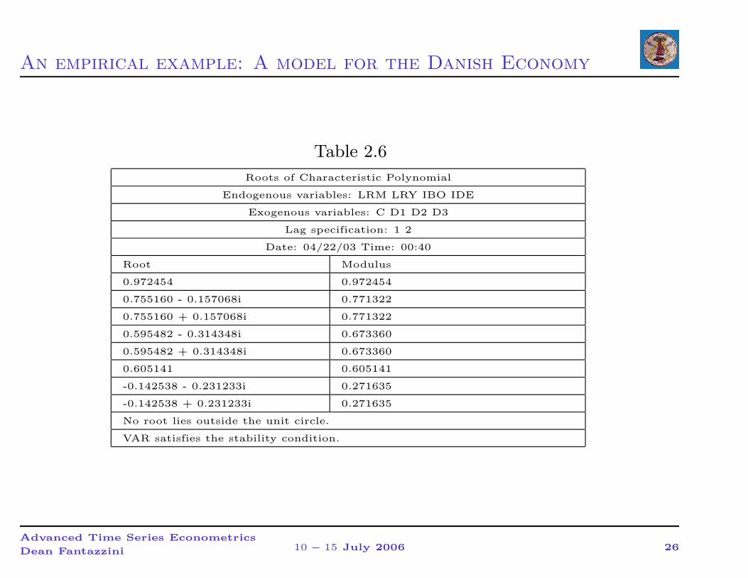
’replicate roots in Table 2.6 (p.25)
freeze(tab26) var1.arroots
show tab26
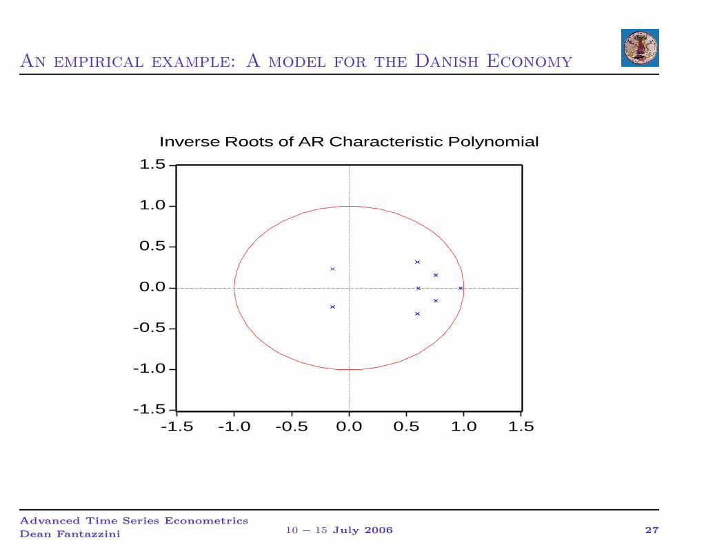
’show roots in unit circle
freeze(gra26) var1.arroots(graph)
show gra26
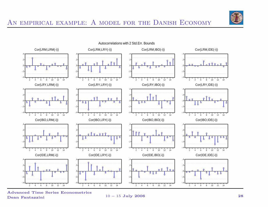
’replicate auto-correlation functions Fig 2.3 (p.28)
’note that eviews graph is transpose of Fig 2.3
freeze(fig23) var1.correl(15,graph)
Advanced Time Series Econometrics
Dean Fantazzini 10 − 15 July 2006 20
An empirical example: A model for the Danish Economy
fig23.options size(4,2)
fig23.align(4,1,1)
show fig23
−→ You should get these results:
Advanced Time Series Econometrics
Dean Fantazzini 10 − 15 July 2006 21
An empirical example: A model for the Danish Economy
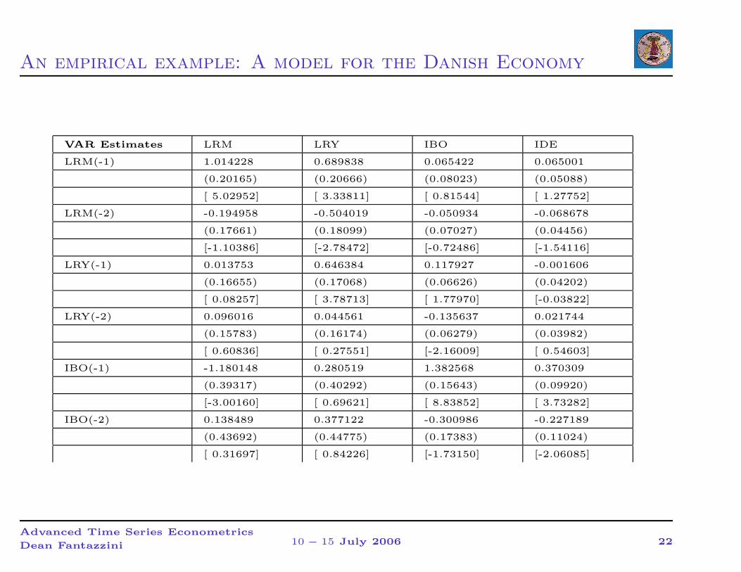
VAR Estimates LRM LRY IBO IDE
LRM(-1) 1.014228 0.689838 0.065422 0.065001
(0.20165) (0.20666) (0.08023) (0.05088)
[ 5.02952] [ 3.33811] [ 0.81544] [ 1.27752]
LRM(-2) -0.194958 -0.504019 -0.050934 -0.068678
(0.17661) (0.18099) (0.07027) (0.04456)
[-1.10386] [-2.78472] [-0.72486] [-1.54116]
LRY(-1) 0.013753 0.646384 0.117927 -0.001606
(0.16655) (0.17068) (0.06626) (0.04202)
[ 0.08257] [ 3.78713] [ 1.77970] [-0.03822]
LRY(-2) 0.096016 0.044561 -0.135637 0.021744
(0.15783) (0.16174) (0.06279) (0.03982)
[ 0.60836] [ 0.27551] [-2.16009] [ 0.54603]
IBO(-1) -1.180148 0.280519 1.382568 0.370309
(0.39317) (0.40292) (0.15643) (0.09920)
[-3.00160] [ 0.69621] [ 8.83852] [ 3.73282]
IBO(-2) 0.138489 0.377122 -0.300986 -0.227189
(0.43692) (0.44775) (0.17383) (0.11024)
[ 0.31697] [ 0.84226] [-1.73150] [-2.06085]
Advanced Time Series Econometrics
Dean Fantazzini 10 − 15 July 2006 22
An empirical example: A model for the Danish Economy
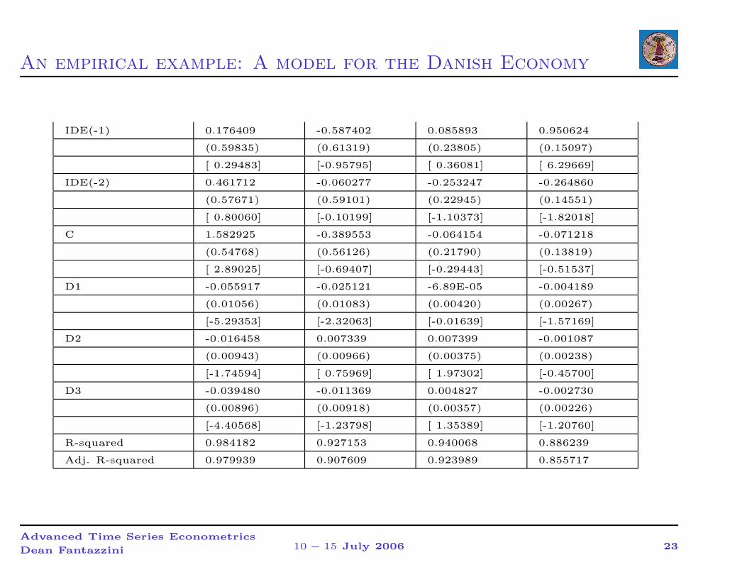
IDE(-1) 0.176409 -0.587402 0.085893 0.950624
(0.59835) (0.61319) (0.23805) (0.15097)
[ 0.29483] [-0.95795] [ 0.36081] [ 6.29669]
IDE(-2) 0.461712 -0.060277 -0.253247 -0.264860
(0.57671) (0.59101) (0.22945) (0.14551)
[ 0.80060] [-0.10199] [-1.10373] [-1.82018]
C 1.582925 -0.389553 -0.064154 -0.071218
(0.54768) (0.56126) (0.21790) (0.13819)
[ 2.89025] [-0.69407] [-0.29443] [-0.51537]
D1 -0.055917 -0.025121 -6.89E-05 -0.004189
(0.01056) (0.01083) (0.00420) (0.00267)
[-5.29353] [-2.32063] [-0.01639] [-1.57169]
D2 -0.016458 0.007339 0.007399 -0.001087
(0.00943) (0.00966) (0.00375) (0.00238)
[-1.74594] [ 0.75969] [ 1.97302] [-0.45700]
D3 -0.039480 -0.011369 0.004827 -0.002730
(0.00896) (0.00918) (0.00357) (0.00226)
[-4.40568] [-1.23798] [ 1.35389] [-1.20760]
R-squared 0.984182 0.927153 0.940068 0.886239
Adj. R-squared 0.979939 0.907609 0.923989 0.855717
Advanced Time Series Econometrics
Dean Fantazzini 10 − 15 July 2006 23
An empirical example: A model for the Danish Economy
Table 2.4
LRM LRY IBO IDE
LRM 1.000000 0.529152 -0.444662 -0.307517
LRY 0.529152 1.000000 -0.082996 -0.237938
IBO -0.444662 -0.082996 1.000000 0.250331
IDE -0.307517 -0.237938 0.250331 1.000000
Advanced Time Series Econometrics
Dean Fantazzini 10 − 15 July 2006 24
An empirical example: A model for the Danish Economy
Table 2.5
RES1 RES2 RES3 RES4
Mean 4.47E-15 -3.94E-17 -3.23E-16 6.27E-17
Median -0.005498 -0.001000 -3.03E-05 -1.53E-05
Maximum 0.051973 0.056657 0.017637 0.014900
Minimum -0.039482 -0.034479 -0.023272 -0.009125
Std. Dev. 0.019222 0.019699 0.007648 0.004850
Skewness 0.551539 0.523993 -0.296653 0.414925
Kurtosis 2.925349 2.912625 3.576072 3.561914
Jarque-Bera 2.699361 2.442215 1.510217 2.218044
Probability 0.259323 0.294903 0.469960 0.329881
Sum 2.37E-13 -2.07E-15 -1.71E-14 3.32E-15
Sum Sq. Dev. 0.019213 0.020178 0.003041 0.001223
Observations 53 53 53 53
Advanced Time Series Econometrics
Dean Fantazzini 10 − 15 July 2006 25
An empirical example: A model for the Danish Economy
Table 2.6
Roots of Characteristic Polynomial
Endogenous variables: LRM LRY IBO IDE
Exogenous variables: C D1 D2 D3
Lag specification: 1 2
Date: 04/22/03 Time: 00:40
Root Modulus
0.972454 0.972454
0.755160 - 0.157068i 0.771322
0.755160 + 0.157068i 0.771322
0.595482 - 0.314348i 0.673360
0.595482 + 0.314348i 0.673360
0.605141 0.605141
-0.142538 - 0.231233i 0.271635
-0.142538 + 0.231233i 0.271635
No root lies outside the unit circle.
VAR satisfies the stability condition.
Advanced Time Series Econometrics
Dean Fantazzini 10 − 15 July 2006 26
An empirical example: A model for the Danish Economy
-1.5
-1.0
-0.5
0.0
0.5
1.0
1.5
-1.5 -1.0 -0.5 0.0 0.5 1.0 1.5
Inverse Roots of AR Characteristic Polynomial
Advanced Time Series Econometrics
Dean Fantazzini 10 − 15 July 2006 27
An empirical example: A model for the Danish Economy
-.4
-.2
.0
.2
.4
2 4 6 8 10 12 14
Cor(LRM,LRM(-i))
-.4
-.2
.0
.2
.4
2 4 6 8 10 12 14
Cor(LRM,LRY(-i))
-.4
-.2
.0
.2
.4
2 4 6 8 10 12 14
Cor(LRM,IBO(-i))
-.4
-.2
.0
.2
.4
2 4 6 8 10 12 14
Cor(LRM,IDE(-i))
-.4
-.2
.0
.2
.4
2 4 6 8 10 12 14
Cor(LRY,LRM(-i))
-.4
-.2
.0
.2
.4
2 4 6 8 10 12 14
Cor(LRY,LRY(-i))
-.4
-.2
.0
.2
.4
2 4 6 8 10 12 14
Cor(LRY,IBO(-i))
-.4
-.2
.0
.2
.4
2 4 6 8 10 12 14
Cor(LRY,IDE(-i))
-.4
-.2
.0
.2
.4
2 4 6 8 10 12 14
Cor(IBO,LRM(-i))
-.4
-.2
.0
.2
.4
2 4 6 8 10 12 14
Cor(IBO,LRY(-i))
-.4
-.2
.0
.2
.4
2 4 6 8 10 12 14
Cor(IBO,IBO(-i))
-.4
-.2
.0
.2
.4
2 4 6 8 10 12 14
Cor(IBO,IDE(-i))
-.4
-.2
.0
.2
.4
2 4 6 8 10 12 14
Cor(IDE,LRM(-i))
-.4
-.2
.0
.2
.4
2 4 6 8 10 12 14
Cor(IDE,LRY(-i))
-.4
-.2
.0
.2
.4
2 4 6 8 10 12 14
Cor(IDE,IBO(-i))
-.4
-.2
.0
.2
.4
2 4 6 8 10 12 14
Cor(IDE,IDE(-i))
Autocorrelations with 2 Std.Err. Bounds
Advanced Time Series Econometrics
Dean Fantazzini 10 − 15 July 2006 28