Applied Physics Research; Vol. 10, No. 6; 2018 ISSN 1916-9639 E-ISSN 1916-9647

Published by Canadian Center of Science and Education

1

Vector Analysis and Optimal Control for the Voltage Regulation of a Weak Power System with Wind Energy and Power Electronics

Nick Schinas1

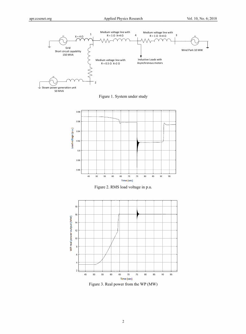
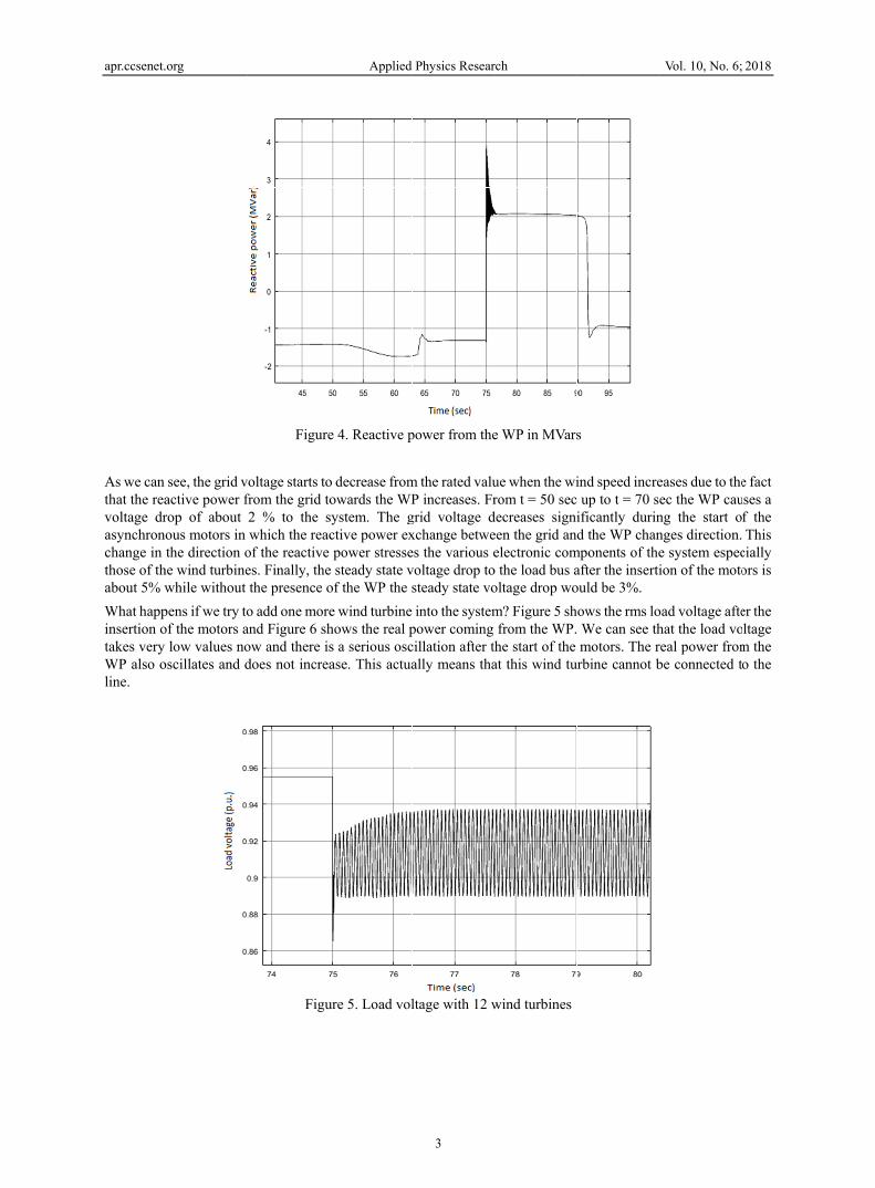
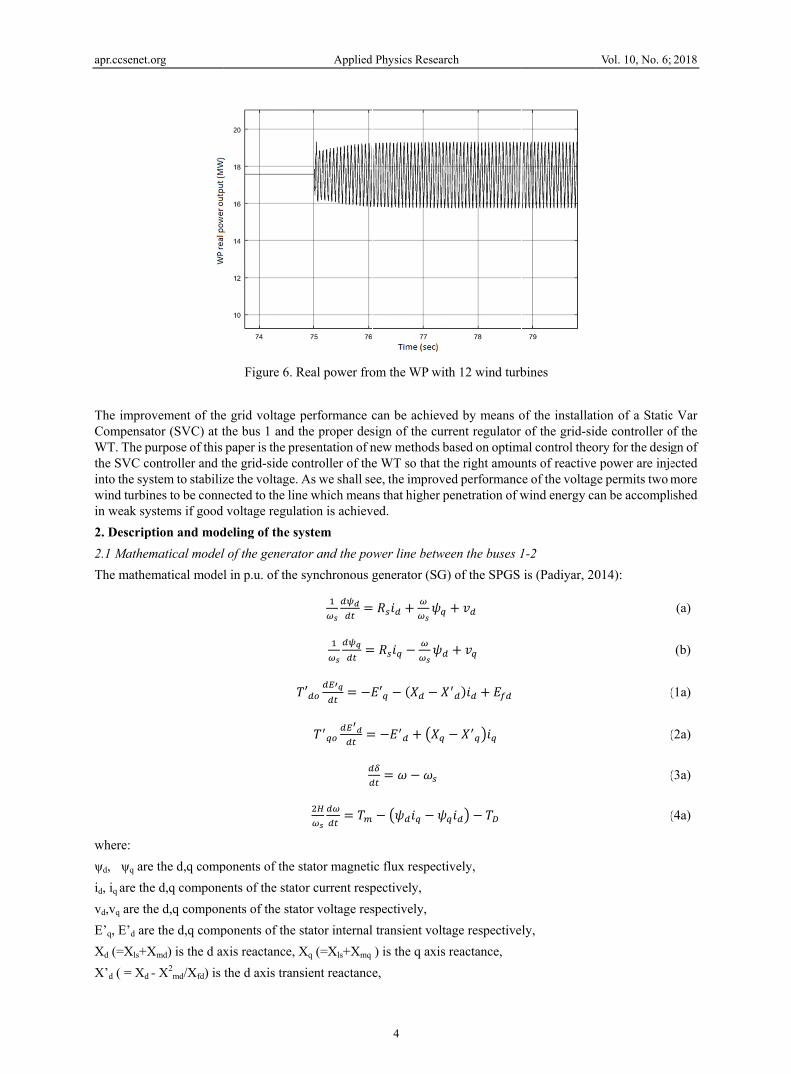
1 Technological Educational Institute of Western Greece, Patras, Greece Correspondence: Nick Schinas, Technological Educational Institute of Western Greece, Patras, Greece. E-mail: nickschinas@gmail.com, nschinas@teiwest.gr Received: September 14, 2018 Accepted: October 1, 2018 Online Published: November 30, 2018 doi:10.5539/apr.v10n6p1 URL: https://doi.org/10.5539/apr.v10n6p1 Abstract This paper deals with the voltage regulation in a weak system which contains large inductive loads and wind turbines using Doubly Fed Induction Generators (FDIGs). The DFIGs demand large amounts of reactive power from the grid and as a result, there is a voltage drop in the system which may be extra deteriorated if large inductive loads and motors are also present in the same line. The problem of the voltage regulation in these cases is treated with the installation of a Static Var Compensator (SVC) besides the capability of the DFIGs to partially regulate the voltage themselves. In this paper, new modeling procedures based on optimal control are developed for the design of the SVC controller and a novel strategy for the grid side converter of the DFIG is presented. The nonlinear system is simulated in the SIMULINK software so that the performance of the new controllers is validated. Keywords: wind turbine, voltage regulation, doubly fed induction generator, optimal control. 1. Introduction The increased need for wind energy development makes the installation of wind turbines in ‘weak’ ac grids necessary. On the other hand, many voltage instability incidents have taken place around the world the last years (Custem & Vournas, 1998; Berizzi, 2004). The distributed generation with wind power stations installed in weak distribution systems may enlarge this problem especially when large inductive loads are connected to the same line. So, voltage regulation has become a major research area in the field of power systems (Chondrogiannis, 2007; Ledesma, 2002; Kesraoui, 2016). This paper deals with the design of the necessary control loops so that good performance of the grid voltage can be attained in a very weak system which contains a wind park (WP) and large inductive loads. The WP consist of wind turbines with Doubly Fed Induction Generators (DFIGs). The DFIGs demand reactive power from the grid. These amounts of reactive power make the grid voltage very sensitive to load variations. The voltage performance can be improved by means of FACTS devices and better voltage controllers inside the DFIG. The system under study is shown in Figure 1. A medium voltage line is connected to the main grid at bus 1 with short circuit capability of 150 MVA. There is a steam power generation system (SPGS) at bus 2 with rated power of 50 MVA and a wind park at bus 3 connected to this line. This system can be a part of a local grid in an island to which wind parks are to be installed. The WP includes 11 wind turbines each with rated real power of 1.5 MW. At bus 4 there are inductive loads with rated power of 2 MVA and power factor 0.9 lagging. These loads also include three asynchronous motors each rated 300 kW. The nominal line voltage of the system is 25 kV. The variation of the reactive power demanded from the WP causes the load voltage at all buses to deviate from the rated values despite the presence of the SPGS in the system. At t = 50 sec there is an increase in the wind speed from 8 m/s to 14 m/s and at t = 75 sec the large induction motors start to operate. Figure 2 shows the rms value of the load voltage at bus 4. The real power produced from the WP is shown in Figure 3 and the reactive power from the WP is shown in Figure 4. The real power production of the SPGS is kept constant at 15 MW.

apr.ccsenet.

Stea

.org

AC

AC

am power generatio50 MVA

GridShort circuit

150 M

1

n unit

d capability

MVA

X = 4 Ω

Fig

Applied

Medium voltaR = 1 Ω

2

Medium voltage lR = 0.5 Ω X=

Figure 1. S

Figure 2. RM

gure 3. Real po

Physics Resear

2

age line withX=4 Ω 4

ine with2 Ω

InAs

System under s

MS load voltage

ower from the

rch

Medium voltage R = 1 Ω X=

nductive Loads withsynchronous motors

study

e in p.u.

WP (MW)

line with4 Ω 3

Win

s

Vol. 10, No. 6;

AC

nd Park 10 MW

2018

apr.ccsenet.

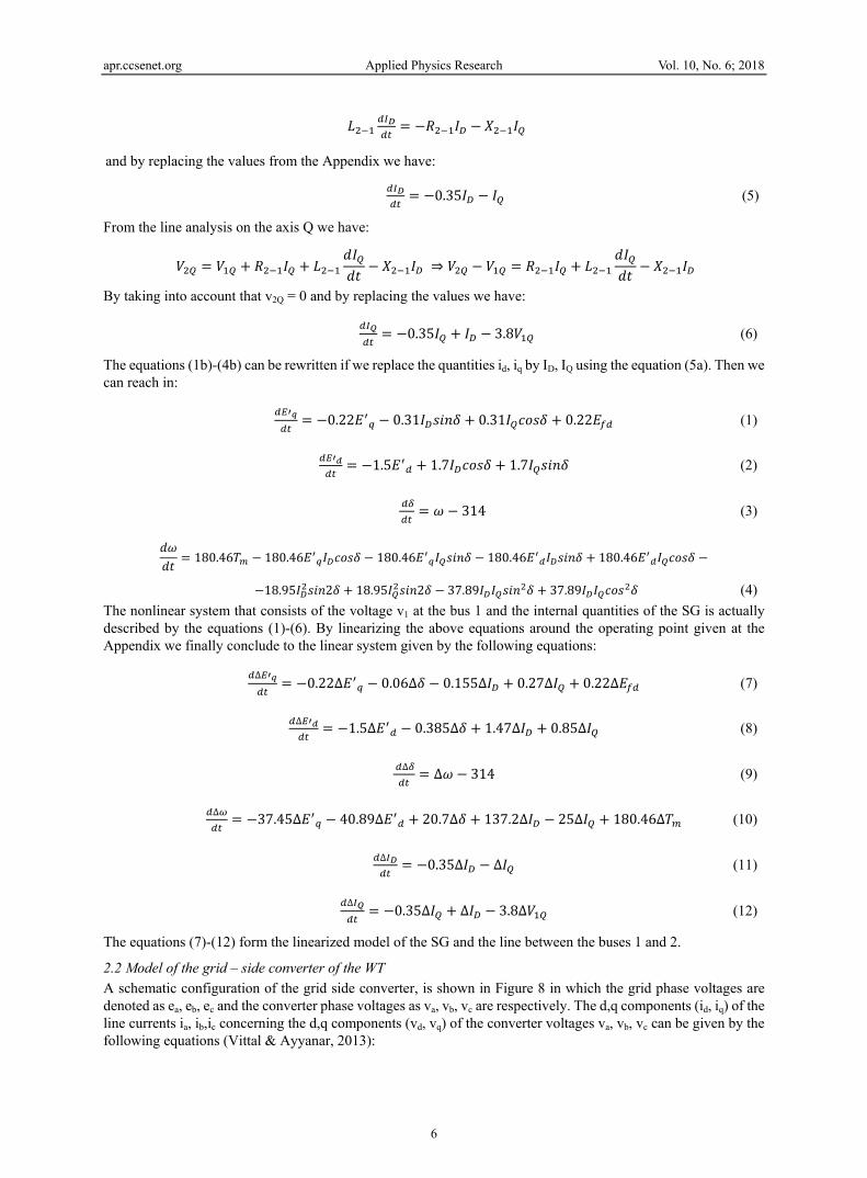
As we can that the reavoltage drasynchronchange in those of thabout 5% wWhat happinsertion otakes very WP also oline.

.org

see, the grid vactive power frop of about

nous motors in the direction o

he wind turbinewhile without pens if we try toof the motors ay low values nooscillates and d

Figure

voltage starts tofrom the grid to2 % to the swhich the reac

of the reactive es. Finally, thethe presence oo add one more

and Figure 6 show and there isdoes not increa

Figu

Applied

e 4. Reactive p

o decrease fromowards the WPsystem. The gctive power expower stresse

e steady state vof the WP the se wind turbine hows the real ps a serious oscase. This actua

ure 5. Load vol

Physics Resear

3

power from the

m the rated valuP increases. Fr

grid voltage dxchange betwees the various evoltage drop tosteady state vo into the systempower coming cillation after thally means tha

ltage with 12 w

rch

e WP in MVars

ue when the wirom t = 50 sec

decreases signieen the grid andelectronic com

o the load bus aoltage drop wom? Figure 5 shfrom the WP.he start of the at this wind tu

wind turbines

s

ind speed incre up to t = 70 sificantly durind the WP chan

mponents of theafter the insertiould be 3%. ows the rms lo We can see thmotors. The r

urbine cannot b

Vol. 10, No. 6;

eases due to theec the WP caung the start onges direction.e system especion of the moto

oad voltage aftehat the load voreal power frombe connected t

2018

e fact uses a f the This

cially ors is

er the oltage m the o the

apr.ccsenet.

The improCompensaWT. The pthe SVC cinto the sywind turbiin weak sy2. Descrip2.1 MathemThe mathe

where: ψd, ψq areid, iq are thvd,vq are thE’q, E’d arXd (=Xls+XX’d ( = Xd

.org

ovement of theator (SVC) at tpurpose of this ontroller and tstem to stabiliznes to be conn

ystems if good ption and modmatical model

ematical model

e the d,q comphe d,q componehe d,q compone the d,q compXmd) is the d ax- X2

md/Xfd) is

Figure 6. R

e grid voltage the bus 1 and paper is the pr

the grid-side coze the voltage.

nected to the linvoltage regula

deling of the sl of the general in p.u. of the

𝑇

ponents of the ents of the statnents of the staponents of the xis reactance, the d axis tran

Applied

Real power fro

performance cthe proper desresentation of nontroller of the As we shall sene which meanation is achievystem tor and the posynchronous g=

=𝑇′ = −𝐸

𝑇 = = 𝑇

stator magnetitor current respator voltage resstator internalXq (=Xls+Xmq

nsient reactance

Physics Resear

4

om the WP wit

can be achievesign of the curnew methods be WT so that thee, the improvens that higher pved.

wer line betwegenerator (SG)= 𝑅 𝑖 + 𝜓

= 𝑅 𝑖 − 𝜓𝐸′ − 𝑋 − 𝑋

= −𝐸 + 𝑋= 𝜔 − 𝜔

− 𝜓 𝑖 − 𝜓ic flux respectipectively, spectively, transient volta) is the q axis e,

rch

th 12 wind turb

ed by means orrent regulator based on optimhe right amouned performancpenetration of w

een the buses 1) of the SPGS + 𝑣 + 𝑣

𝑋 𝑖 + 𝐸 − 𝑋 𝑖

𝑖 − 𝑇

ively,

age respectivereactance,

bines

of the installatof the grid-sid

mal control theonts of reactivee of the voltagwind energy ca

1-2 is (Padiyar, 20

ly,

Vol. 10, No. 6;

tion of a Staticde controller oory for the desi power are inje

ge permits two an be accompli

014):

(

(

(

(

2018

c Var of the gn of ected more ished

(a)

(b)

(1a)

(2a)

(3a)

(4a)

apr.ccsenet.org Applied Physics Research Vol. 10, No. 6; 2018

5

X’q ( = Xq - X2mq/X1q) is the q axis transient reactance,

ω is the rotor electrical angular speed, 𝜔 is the electrical speed of the magnetic flux, δ is the power angle, H is the inertia constant, Tm is the mechanical torque, TD is the damping torque (being neglected from now on). Finally, T’do, T’qo are time constants on field and damper winding respectively (we consider the machine to have one damping winding on q axis) and Rs is the stator resistance. By neglecting the equations regarding the stator magnetic fluxes (equations (a) and (b) above) and replacing the relevant values from the Appendix we have:

= −0.22 𝐸′ − 0.31𝑖 + 0.22𝐸 (1b)

= −1.5 𝐸 + 1.7 𝑖 (2b)

= 𝜔 − 314 (3b)

It also is: 𝜓 = −𝑥 𝑖 + 𝐸 , 𝜓 = −𝑥 𝑖 − 𝐸′ By replacing to (4a) we finally reach in:

= 180.46 𝑇 − 180.46 𝐸 𝑖 − 180.46 𝐸 𝑖 + 37.89𝑖 𝑖 (4b)

As we have already seen, the SPGS is connected to the bus 2 and there is a small line up to the main bus 1. The Figure 7 depicts the vectors of the voltages at the buses. The voltage v2 at the bus 2 will be a little ahead of the voltage v1 at the bus 1 (approximately 3 degrees). We consider the main axes D, Q and the axes d, q internally in the synchronous generator to which the various quantities of the SG have been analyzed in the equations (1b)-(4b). We arbitrarily consider that the voltage v2 is lying on the D axis. The stator current i of the SG with its components id, iq onto the axes d, q is also the current I of the line between the buses 2 and 1 with the components ID, IQ onto the axes D, Q respectively. It is (Pai et al., 2014): 𝑖 = 𝐼 𝑠𝑖𝑛𝛿 − 𝐼 𝑐𝑜𝑠𝛿, 𝑖 = 𝐼 𝑐𝑜𝑠𝛿 + 𝐼 𝑠𝑖𝑛𝛿 (5a)

D

Q

V1

V2

q

d

δ

iq

id

ID

IQ

Figure 7. Vector analysis of the system

Applying the D-Q analysis on the line between the buses 2 and 1 we have firstly on the D axis: 𝑉 = 𝑉 + 𝑅 𝐼 + 𝐿 + 𝑋 𝐼 ⇒ 𝑉 − 𝑉 = 𝑅 𝐼 + 𝐿 + 𝑋 𝐼

Due to the small value of the angle between v1 and v2 it is approximately: 𝑉 − 𝑉 ≈ 0. So from the previous equation we conclude to:

apr.ccsenet.org Applied Physics Research Vol. 10, No. 6; 2018

6

𝐿 = −𝑅 𝐼 − 𝑋 𝐼

and by replacing the values from the Appendix we have:

= −0.35𝐼 − 𝐼 (5)

From the line analysis on the axis Q we have: 𝑉 = 𝑉 + 𝑅 𝐼 + 𝐿 𝑑𝐼𝑑𝑡 − 𝑋 𝐼 ⇒ 𝑉 − 𝑉 = 𝑅 𝐼 + 𝐿 𝑑𝐼𝑑𝑡 − 𝑋 𝐼

By taking into account that v2Q = 0 and by replacing the values we have:

= −0.35𝐼 + 𝐼 − 3.8𝑉 (6)

The equations (1b)-(4b) can be rewritten if we replace the quantities id, iq by ID, IQ using the equation (5a). Then we can reach in:

= −0.22𝐸 − 0.31𝐼 𝑠𝑖𝑛𝛿 + 0.31𝐼 𝑐𝑜𝑠𝛿 + 0.22𝐸 (1)

= −1.5𝐸 + 1.7𝐼 𝑐𝑜𝑠𝛿 + 1.7𝐼 𝑠𝑖𝑛𝛿 (2)

= 𝜔 − 314 (3) 𝑑𝜔𝑑𝑡 = 180.46𝑇 − 180.46𝐸 𝐼 𝑐𝑜𝑠𝛿 − 180.46𝐸 𝐼 𝑠𝑖𝑛𝛿 − 180.46𝐸 𝐼 𝑠𝑖𝑛𝛿 + 180.46𝐸 𝐼 𝑐𝑜𝑠𝛿 −

−18.95𝐼 𝑠𝑖𝑛2𝛿 + 18.95𝐼 𝑠𝑖𝑛2𝛿 − 37.89𝐼 𝐼 𝑠𝑖𝑛 𝛿 + 37.89𝐼 𝐼 𝑐𝑜𝑠 𝛿 (4) The nonlinear system that consists of the voltage v1 at the bus 1 and the internal quantities of the SG is actually described by the equations (1)-(6). By linearizing the above equations around the operating point given at the Appendix we finally conclude to the linear system given by the following equations:

∆ = −0.22∆𝐸 − 0.06∆𝛿 − 0.155∆𝐼 + 0.27∆𝐼 + 0.22∆𝐸 (7)

∆ = −1.5∆𝐸 − 0.385∆𝛿 + 1.47∆𝐼 + 0.85∆𝐼 (8)

∆ = ∆𝜔 − 314 (9)

∆ = −37.45∆𝐸 − 40.89∆𝐸 + 20.7∆𝛿 + 137.2∆𝐼 − 25∆𝐼 + 180.46∆𝑇 (10)

∆ = −0.35∆𝐼 − ∆𝐼 (11)

∆ = −0.35∆𝐼 + ∆𝐼 − 3.8∆𝑉 (12)

The equations (7)-(12) form the linearized model of the SG and the line between the buses 1 and 2.

2.2 Model of the grid – side converter of the WT A schematic configuration of the grid side converter, is shown in Figure 8 in which the grid phase voltages are denoted as ea, eb, ec and the converter phase voltages as va, vb, vc are respectively. The d,q components (id, iq) of the line currents ia, ib,ic concerning the d,q components (vd, vq) of the converter voltages va, vb, vc can be given by the following equations (Vittal & Ayyanar, 2013):

apr.ccsenet.

The modelchoice of treplacing t

As there ifrequency the paramesystem and

3. Control

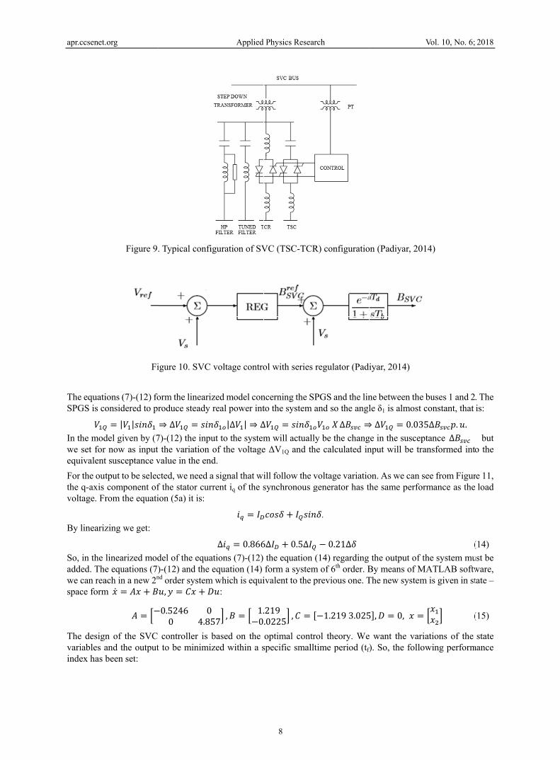
3.1 SVC CIn order foinstallationwhich fastThere is aregulates tinto the sysignals in There are voltage at

that is, the variation othe bus 1.

.org

Fi𝐿 𝑑𝑑ling of the convthe WT d,q, axthe p.u. values𝑑𝑖𝑑𝑡 =is the SPGS inis assumed to

eter ωs has beed not an input

∆l SYSTEM DE

Controller Desior the load voltn is proposed at power factor a main voltagethe right suscepystem. A blockthe decision ono such signathe bus 1 to ch

variation of thof the suscepta

igure 8. Grid s𝑑𝑖𝑑𝑡 = −𝑅 𝑖 +verter of the Wxes is arbitrarys from the App= −0.01𝑖 + 𝑖n our system be constant an

en set equal to and so the line= −0.01∆𝑖ESIGN

ign age to be kept at the bus 1 of timprovement e controller wptance being cok diagram of Sof the right susals in our studyhange. If only

he magnitude oance of the SVC

Applied

ide converter c+ 𝜔 𝐿 𝑖 + 𝑒WT and its conty. The grid volpendix we reac𝑖 + 6.67𝑒 −with installed

nd that it does n1. Besides, theearized model + ∆𝑖 − 6.67constant underthe system. Thcan be achiev

which accordinonnected to theSVC voltage csceptance (B) y. The connecthe fundament∆𝑉

of the voltage aC (ΔBsvc). X

Physics Resear

7

configuration (− 𝑣 , 𝐿 𝑑𝑖𝑑𝑡trol design hasltage e has bee

ch in the follow− 6.67𝑣 , 𝑑𝑖𝑑𝑡d capacity mucnot depend on te parameter ed for the control7∆𝑣 , ∆ =r reactive powhe SVC is actued. Figure 9 sh

ng to the deviae bus and so th

control is depicof the SVC co

cted susceptanctal component≅ 𝑋∆𝐵 ,

at the bus whereis the equivale

rch

(Vittal & Ayya= −𝑅 𝑖 − 𝜔 nothing to do en chosen to liwing equations

𝑡 = −0.01𝑖 −ch larger that the real power is considered tl design of the= −0.01∆𝑖 −

wer from the WPually a device whows a typicalation of the b

he right amouncted in Figure ontrol, like thece at the bus 1t of Vsvc is con

e the SVC is inent Thevenin re

anar, 2013) 𝜔 𝐿 𝑖 − 𝑣 with the rest o

ie on the d axis: − 𝑖 − 6.67𝑣

the rated outpcoming from tto be a disturba

e grid side conv∆𝑖 − 6.67∆𝑣P and the load

with variable sul SVC (TSC-Tbus voltage front of reactive po

10. There cane signals Vs sh1 will force thnsidered, we c

nstalled (i.e. buesistance of th

Vol. 10, No. 6;

of the system, sis and so eq = 0

put of the WPthe WP. As a reance for the coverter is given 𝑣 (

variations, an usceptance thr

TCR) configuraom the rated vower being insn be more auxihown in Figure magnitude o

can assume tha

us 1) depends ohe grid as seen

2018

so the 0. By

P, the esult,

ontrol by:

(13)

SVC rough ation. value erted iliary e 10.

of the at:

on the from

apr.ccsenet.

The equatiSPGS is co𝑉In the modwe set for equivalentFor the outthe q-axis voltage. Fr

By lineariz

So, in the added. Thewe can reaspace form

The designvariables aindex has b

.org

Figure 9.

Fi

ions (7)-(12) foonsidered to pr= |𝑉 |𝑠𝑖𝑛𝛿del given by (7r now as input t susceptance vtput to be seleccomponent ofrom the equati

zing we get:

linearized mode equations (7)ach in a new 2n

m 𝑥 = 𝐴𝑥 + 𝐵 𝐴 = −

n of the SVC and the outputbeen set:

. Typical confi

igure 10. SVC

orm the lineariroduce steady ⇒ Δ𝑉 = 𝑠𝑖𝑛

7)-(12) the inputhe variation

value in the encted, we need af the stator curion (5a) it is:

del of the equa)-(12) and the nd order system𝑢, 𝑦 = 𝐶𝑥 + 𝐷−0.5246 00 4.85

controller is t to be minimi

Applied

iguration of SV

voltage contro

zed model conreal power int𝑛𝛿 |Δ𝑉 | ⇒ Δut to the systemof the voltaged. a signal that wirrent iq of the s

𝑖 = 𝐼 Δ𝑖 = 0.866

ations (7)-(12) equation (14)

m which is equi𝐷𝑢: 057 , 𝐵 = 1.−0based on the

ized within a s

Physics Resear

8

VC (TSC-TCR

ol with series r

ncerning the SPto the system aΔ𝑉 = 𝑠𝑖𝑛𝛿m will actuallye ΔV1Q and the

ill follow the vsynchronous g

𝑐𝑜𝑠𝛿 + 𝐼 𝑠𝑖𝑛6Δ𝐼 + 0.5Δ𝐼

the equation (form a system

ivalent to the p

.219.0225 , 𝐶 =optimal contro

specific smallt

rch

R) configuratio

regulator (Padi

PGS and the linand so the angl𝑉 𝑋 Δ𝐵 ⇒y be the change calculated in

voltage variatiogenerator has th

𝛿.

− 0.21Δ𝛿 (14) regarding

m of 6th order. Bprevious one. T

−1.219 3.025ol theory. Wetime period (tf)

on (Padiyar, 20

iyar, 2014)

ne between thele δ1 is almost ⇒ Δ𝑉 = 0.03

ge in the suscepnput will be tr

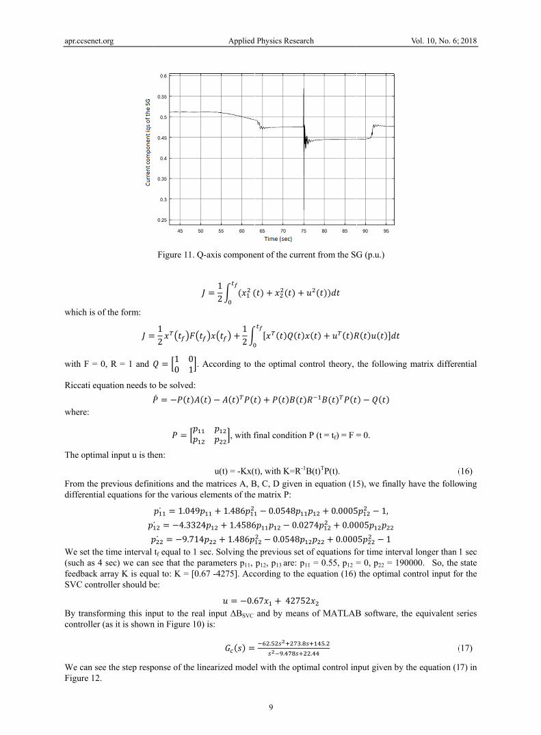
on. As we can she same perfo

the output of By means of MThe new system

5 , 𝐷 = 0, 𝑥 =e want the varf). So, the follo

Vol. 10, No. 6;

014)

e buses 1 and 2constant, that 35Δ𝐵 𝑝. 𝑢.

ptance Δ𝐵 ransformed int

see from Figurormance as the

(the system mu

MATLAB softwm is given in st

= 𝑥𝑥 (

riations of the owing perform

2018

. The is:

but o the

re 11, load

(14) ust be ware, tate –

(15)

state mance

apr.ccsenet.

which is o

with F = 0

Riccati equ

where:

The optim

From the pdifferentia

We set the(such as 4feedback aSVC contr

By transfocontroller

We can seFigure 12.

.org

f the form: 𝐽 =0, R = 1 and

uation needs to𝑃mal input u is th

previous definal equations for

𝑝𝑝e time interval 4 sec) we can sarray K is equroller should b

orming this inp(as it is shown

ee the step resp

Figure 11. Q-

𝐽= 12 𝑥 𝑡 𝐹 𝑡

𝑄 = 1 00 1 . A

o be solved: 𝑃 = −𝑃 𝑡 𝐴𝑃 = 𝑝𝑝

hen:

nitions and the r the various e𝑝 = 1.049𝑝= −4.3324𝑝 = −9.714tf equal to 1 se

see that the paal to: K = [0.6

be:

put to the realn in Figure 10)

ponse of the lin

Applied

-axis compone

𝐽 = 12 𝑥𝑥 𝑡 + 12

According to t

𝑡 − 𝐴 𝑡 𝑃 𝑡𝑝𝑝 , with f

u(t) = -Kx(tmatrices A, Blements of the𝑝 + 1.486𝑝4𝑝 + 1.4586𝑝 + 1.486𝑝ec. Solving thearameters p11, 67 -4275]. Acc

𝑢 = −0.6l input ΔΒSVC ) is:

𝐺 𝑠 =nearized mode

Physics Resear

9

ent of the curre

𝑡 + 𝑥 𝑡 +𝑥 𝑡 𝑄 𝑡 𝑥

the optimal co

𝑡 + 𝑃 𝑡 𝐵 𝑡final condition

t), with K=R-1

B, C, D given ie matrix P: − 0.0548𝑝6𝑝 𝑝 − 0.02− 0.0548𝑝e previous set p12, p13 are: p1

cording to the

67𝑥 + 4275and by means

. ..el with the opti

rch

ent from the SG

𝑢 𝑡 𝑑𝑡

𝑥 𝑡 + 𝑢 𝑡 𝑅ontrol theory,

𝑅 𝐵 𝑡 𝑃 𝑡n P (t = tf) = F =

B(t)TP(t). in equation (15

𝑝 + 0.0005274𝑝 + 0.00𝑝 + 0.000of equations f

11 = 0.55, p12 =equation (16)

2𝑥 s of MATLAB

..

imal control in

G (p.u.)

𝑅 𝑡 𝑢 𝑡 𝑑𝑡

the following

𝑡 − 𝑄 𝑡

= 0.

5), we finally

5𝑝 − 1, 005𝑝 𝑝 05𝑝 − 1 for time interva= 0, p22 = 190the optimal co

B software, th

nput given by t

Vol. 10, No. 6;

matrix differe

(have the follo

al longer than 0000. So, the ontrol input fo

he equivalent s

(

the equation (1

2018

ential

(16) wing

1 sec state

or the

series

(17)

17) in

apr.ccsenet.

We can se3.2 Grid siThe linear

Due to theconclude t

and we con

be equal to

We set the

𝐻In order to

By substitu𝐻 𝑥We solve t

Now let’s to be indep

.org

Fig

e that the systeide converter cized model is g

𝑥 =e nature of the to a controller

nsider the opti

o: 𝐽∗ = 𝑘𝑥 +e Hamiltonian

𝑥 𝑡 , 𝑢 𝑡 , 𝐽∗𝐻 𝑥 𝑡 , 𝑢 𝑡 , 𝐽o have optimiza

ution to the pr𝑡 , 𝑢 𝑡 , 𝐽∗ =𝐻 𝑥 𝑡the HJB equati

𝐻 𝑥 𝑡 , 𝑢 𝑡recall that x1 =pendent on the

gure 12. Step re

em output getscontrol designgiven by the e𝑥 = 𝑥𝑥 =−0.01𝑥 + 𝑥above equatiovery easily. W𝐽 = 𝑉imal performan

+ 𝑘𝑥 , then i

equation as:

= 𝑉 𝑥 𝑡 , 𝑢 𝑡𝐽𝑥∗ = 𝑥 + 𝑥ation there mu𝜕𝐻𝜕𝑢 = 0 ⇒evious we hav𝑥 + 𝑥 + 11.1𝑡 , 𝑢 𝑡 , 𝐽𝑥∗ =ion: 𝑡 , 𝐽𝑥∗ + 𝐽𝑡∗ = 0

= Δid, x2 = Δiq. e changes in th

Applied

esponse of the

s the desired va quations (13). = ∆𝑖∆ , 𝑢 =− 6.67𝑢 = 𝑓

ons we can woWe set the perfo𝑉 𝑥 𝑡 , 𝑢 𝑡 𝑑

nce index to

it is: 𝐽∗ = ∗∗

+ 𝐽∗ 𝑓𝑓 = 𝑥+ 𝑢 + 𝑢 −ust be: ⇒ 𝑢∗ = 3.335𝑘ve: 12𝑘 𝑥 + 11.121 − 11.12𝑘0 ⇒ 1 − 11.12We want the c

he q axis (whi

Physics Resear

10

linearized mo

alue in 0.1 sec

In state space 𝑢𝑢 = ∆𝑣∆𝑣 , 𝑓 , 𝑥 = −rk with the Ha

ormance index𝑑𝑡 = 𝑥 + 𝑥∗∗ = 𝑘𝑥𝑘𝑥 , 𝐽∗

𝑥 + 𝑥 + 𝑢 +0.01𝑘𝑥 − 6.6𝑘𝑥 , 𝜕𝐻𝜕𝑢 = 0 ⇒2𝑘 𝑥 − 0.01𝑘𝑥− 0.01𝑘 𝑥 +2𝑘 − 0.01𝑘 𝑥changes in the ch is responsib

rch

odel under opti

c.

form if we set

then we can w−0.01𝑥 − 𝑥 −amilton - Jacobx as: 𝑥 + 𝑢 + 𝑢∗ = ∗ = 0 .

𝑢 + 𝑘𝑥 𝑘𝑥67𝑘𝑥 𝑢 − 0.0⇒ 𝑢∗ = 3.335𝑥 − 0.01𝑘𝑥 −+ 1 − 11.12𝑘𝑥 + 1 − 11.d axis (which ble for the rea

imal control.

t

write: − 6.67𝑢 = 𝑓bi – Bellman (

𝑑𝑡

−0.01𝑥 + 𝑥−𝑥 − 0.01𝑥001𝑘𝑥 − 6.65𝑘𝑥 . − 22.24𝑘 𝑥 −𝑘 − 0.01𝑘 𝑥.12𝑘 − 0.01𝑘is responsible ctive power).

Vol. 10, No. 6;

(HJB) equation

− 6.67𝑢− 6.67𝑢 67𝑘𝑥 𝑢

22.24𝑘 𝑥 ⇒

𝑘 𝑥 = 0 (for the real poIn other words

2018

n and

(18) ower) s, the

apr.ccsenet.

input u mu(18) to be

We keep th

A very sim

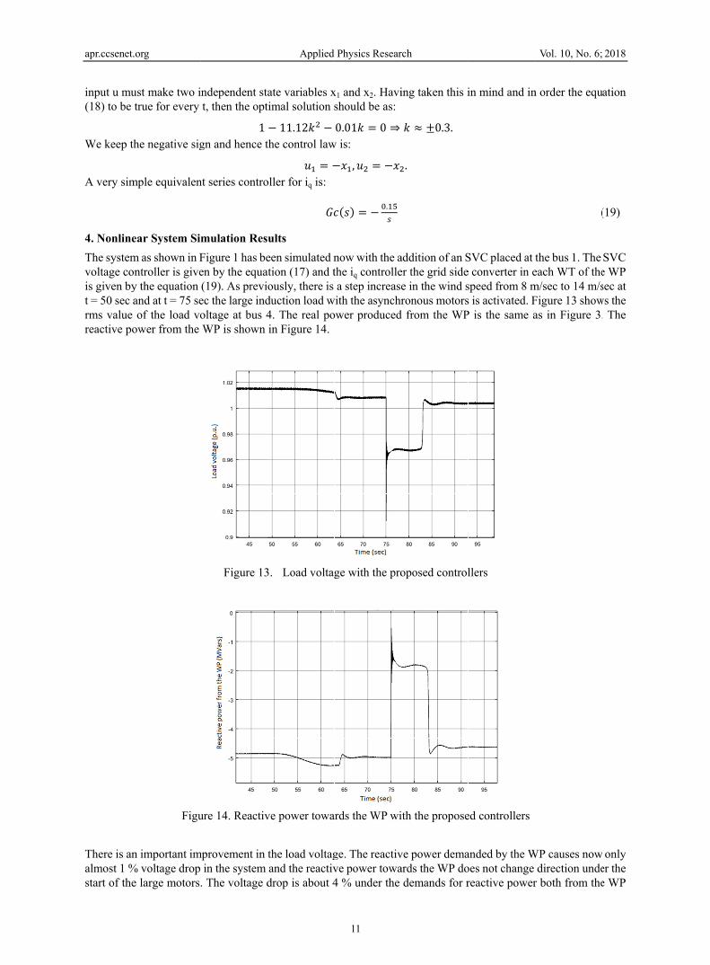
4. NonlineThe systemvoltage cois given byt = 50 sec arms value reactive po

There is analmost 1 %start of the

.org

ust make two itrue for every

he negative sig

mple equivalen

ear System Sim as shown in Fontroller is givey the equation and at t = 75 seof the load vo

ower from the

Figu

n important im% voltage drop e large motors

independent stat, then the opt1

gn and hence t

nt series contro

mulation ResFigure 1 has been by the equa(19). As previec the large indoltage at bus 4WP is shown

Figure 13

ure 14. Reactiv

mprovement in in the system

. The voltage d

Applied

ate variables xtimal solution s− 11.12𝑘 −the control law𝑢 = −oller for iq is: 𝐺𝑐ults een simulated nation (17) and tously, there is duction load w4. The real poin Figure 14.

3. Load voltag

ve power towa

the load voltagand the reactivdrop is about 4

Physics Resear

11

x1 and x2. Havishould be as: 0.01𝑘 = 0 ⇒

w is: −𝑥 , 𝑢 = −𝑥𝑐 𝑠 = − .

now with the athe iq controllea step increase

with the asynchrower produced

ge with the pro

ards the WP wi

ge. The reactivve power towa4 % under the

rch

ing taken this i

𝑘 ≈ 0.3. .

addition of an Ser the grid sidee in the wind sronous motors

d from the WP

oposed control

ith the propose

ve power demaards the WP dodemands for r

in mind and in

SVC placed at te converter in espeed from 8 ms is activated. FP is the same a

llers

ed controllers

anded by the Woes not change reactive power

Vol. 10, No. 6;

n order the equ

(

the bus 1. The each WT of them/sec to 14 m/sFigure 13 showas in Figure 3.

WP causes nowdirection unde

r both from the

2018

ation

(19)

SVC e WP sec at

ws the . The

only er the e WP

apr.ccsenet.

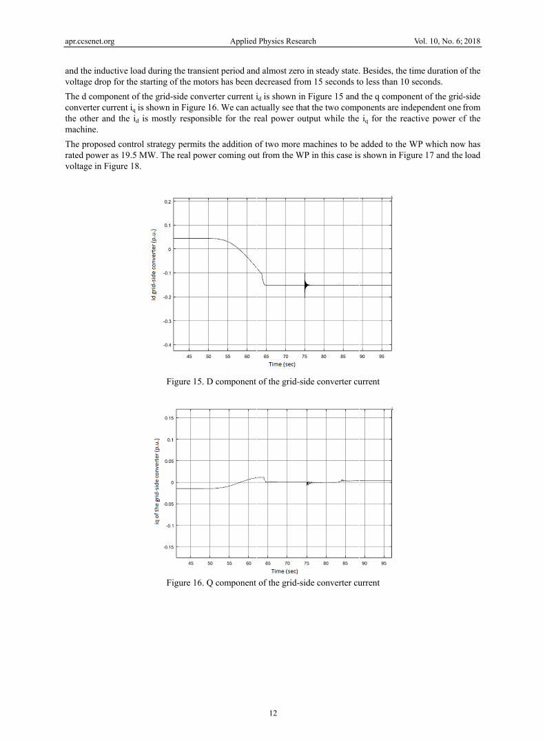
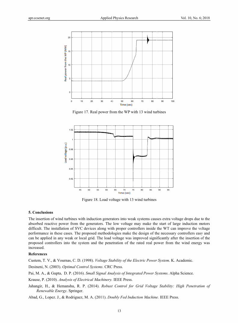
and the indvoltage droThe d comconverter cthe other amachine. The proporated powevoltage in

.org

ductive load duop for the start

mponent of the current iq is shand the id is m

osed control strer as 19.5 MWFigure 18.

uring the transting of the motgrid-side convown in Figure

mostly respons

rategy permitsW. The real pow

Figure 15.

Figure 16.

Applied

ient period andtors has been dverter current i16. We can ac

sible for the r

s the addition ower coming ou

D component

Q component

Physics Resear

12

d almost zero idecreased fromid is shown in Fctually see thatreal power out

of two more mut from the WP

of the grid-sid

of the grid-sid

rch

in steady state.m 15 seconds toFigure 15 and t the two comptput while the

machines to be P in this case is

de converter cu

de converter cu

. Besides, the to less than 10 the q compon

ponents are indiq for the rea

added to the Ws shown in Figu

urrent

urrent

Vol. 10, No. 6;

time duration oseconds.

nent of the griddependent one active power o

WP which nowure 17 and the

2018

of the

d-side from

of the

w has load

apr.ccsenet.

5. ConclusThe insertiabsorbed rdifficult. Tperformancan be appproposed increased. ReferenceCustem, TDesineni, NPai, M. A.Krause, P.Jahangir,

RenewAbad, G.,

.org

sions ion of wind tureactive poweThe installationnce in these caplied in any wcontrollers int

es T. V., & Vourn

N. (2003). Op, & Gupta, D. (2010). AnalyH., & Hemanwable Energy.Lopez. J., & R

Figure 17.

Figur

urbines with inder from the gen of SVC devses. The propo

weak or local gto the system

nas, C. D. (199timal Control . P. (2016). Smysis of Electricnshu, R. P. (2. Springer. Rodriguez, M.

Applied

Real power fr

re 18. Load vo

duction generaenerators. The vices along witosed methodol

grid. The load and the pene

8). Voltage StaSystems. CRC

mall Signal Anacal Machinery.2014). Robust

A. (2011). Do

Physics Resear

13

om the WP wi

oltage with 13

ators into weaklow voltage m

th proper contlogies make thvoltage was im

etration of the

ability of the EC Press. alysis of Integr IEEE Press.

t Control for

oubly Fed Indu

rch

ith 13 wind tur

wind turbines

k systems causmay make thetrollers inside the design of thmproved signie rated real po

Electric Power

rated Power Sy

Grid Voltage

uction Machine

rbines

ses extra voltae start of largethe WT can im

he necessary cificantly after tower from the

r System. K. Ac

Systems. Alpha

e Stability: Hi

e. IEEE Press.

Vol. 10, No. 6;

age drops due te induction mmprove the voontrollers easythe insertion o

e wind energy

cademic.

Science.

igh Penetratio

2018

to the motors oltage y and of the y was

on of

apr.ccsenet.org Applied Physics Research Vol. 10, No. 6; 2018

14

Robert, F. S. (1993). Optimal Control and Estimation. Dover publications. Vijay, V., & Raja, A. (2012). Grid Integration and Dynamic Impact of Wind Energy. Springer. Kesraoui, M., & Chaib, A. (2016). Grid voltage local regulation by a doubly fed induction generator-based wind

turbine. Wind Engineering, 41(1), 13-25. Rui, S., & Rui, X. (2015). The design and analysis of wind turbine based on differential speed regulation. Wind

Engineering, 230(2), 221-229. Yu, L., & Zhenlan, D. (2012). Improvement of the low-voltage ride-through capability of doubly fed Induction

Generator Wind Turbines. Wind Engineering, 36(5), 535-551. Appendix Table 1. WT parameters (Abad et al., 2011)

Nominal active power PN 1.5 MW Nominal electrical torque TelN or Tg 9555 Nm Stator voltage VSN 690 V Nominal generator speed ηgo 1800 rpm Speed range of generator 900-1850 rpm Pole pairs 4 Blades diameter d 60 m Nominal wind speed VwN 12 m/sec Maximum power coefficient Cp 0.44 Air density 1.125 kg/m3 Nominal turbine speed ηto 22.5 rpm Speed range of turbine speed 9-23 rpm TSR optimum 5.43 Grid side components (mΩ) Rg = 0.33 Xg = 31.4

Table 2. Medium voltage lines

Rated voltage VN 25 kV Inductive reactance Xo 0.4 Ω/km Resistance Ro 0.1 Ω/km Length between buses 1-2 5 km Length between buses 1-4 and 3-4 10 km

Table 3. Synchronous generator parameters (Pai et al., 2016)

Rated voltage VN 11 kV D axis open circuit time constant Tdo’ 4.5 sec Rated power SN 50 MVA Q axis open circuit time constant Tqo’ 0.67 sec Transient reactance on d axis Xd’ 0.25 p.u. Inertia constant H 0.87 sec Reactance on d axis Xd 1.65 p.u. Stator resistance Rs 0.0045 p.u. Transient reactance on q axis Xq’ 0.46 p.u. Power angle operating point δo =300 Reactance on q axis Xq 1.59 p.u. Bus 1 voltage operating point V1qo=-0.052 p.u. Subt. int.voltage on q axis Eq’ operating point E’qo=0.68 p.u. Line current on D axis operating point IDo=0.28 p.u. Subt. int.voltage on d axis Ed’ operating point E’do=0.22 p.u. Line current on Q axis operating point IQo=-0.1 p.u.

Copyrights Copyright for this article is retained by the author(s), with first publication rights granted to the journal. This is an open-access article distributed under the terms and conditions of the Creative Commons Attribution license (http://creativecommons.org/licenses/by/4.0/).