Embed Size (px)
Citation preview


PU,M
VECTOR ANALYSISAND THE
THEORY OF RELATIVITY
BY
FRANCIS D. MURNAGHAN, M.A. (N.U.I.), PH.D.
Associate Professor of Applied Mathematics, Johns Hopkins University.
546G58
BALTIMORE
THE JOHNS HOPKINS PRESS
1922

JL\\t ^jnuitay ~itinting Company
lETTEIPIESS AND OFFSET

One of the most striking effects of the publication of Ein-
stein's papers on generalized relativity and of the discussions
which arose in connection with the subsequent astronomical
observations was to make students of physics renew their study
of mathematics. At first they attempted to learn simply the
technique, but soon there was a demand to understand more;
real mathematical insight was sought. Unfortunately there
were no books available, not even papers.
Dr. Murnaghan's little book is a most successful attempt to
supply what is a definite need. Every physicist can read it with
profit. He will learn the meaning of a vector for the first time.
He will learn methods which are available for every field of
mathematical physics. He will see which of the processes used
by Einstein and others are strictly mathematical and which are
physical. Every chapter is illuminating, and the treatment of
the subject is that of a student of mathematics and is not de-
veloped ad hoc. The extension of surface and line integrals is
most interesting for physicists and the discussion of the space
relations in a four-dimensional geometry is one most needed.
This is specially true concerning the case of point-symmetrywhich forms the basis of Einstein's formulae for gravitation as
applied to the solar system.
I feel personally that I owe to this book a great debt. I have
read it with care and shall read it again. It has given me a
definiteness of understanding which I never had before, and a
vision of a field of knowledge which before was remote.
JOSEPH S. AMES.JOHNS HOPKINS UNIVERSITY,
June 1, 1921.
in


CONTENTSPAGE
Introduction 1
CHAPTER ONE
THE TENSOR CONCEPT
Spreads in Space of n Dimensions 4
Integral over a Spread of One Dimension 6
Integral over a Spread of Two or More Dimensions 7
Transformation of Coordinates 11
Covariant Tensors of Arbitrary Rank 15
Contravariant Tensors 16
Mixed Tensors 17
Invariants 18
CHAPTER TWOTHE ALGEBRA OF TENSORS
The Rule of Linear Combination 21
The Rule of Interchange of Order of Components 22
The Simple Tensor Product 24
The Outer Product of Two Tensors of Rank One 25
The Rule of Composition or Inner Multiplication 25
Converse of the Rule of Composition 27
Applications of the Four Rules 29
Stokes' Generalised Lemma 33
Examples 34
The Curl of a Covariant Tensor of Rank One 34
Integral of an "Exact Differential" 35
Maxwell's Electromagnetic Potential 37
Lorentz's Retarded Potential 38
v

VI CONTENTS
PAGE
CHAPTER THREE
THE METRICAL CONCEPT
The Metrical Idea in Geometry 40
The Reciprocal Quadratic Differential Form 41
The Transformation of the Determinant of the Form 43
The Invariant of Space-Content 46
The Divergence of a Contravariant Tensor of Rank One ... 47
The Magnitude of a Covariant Tensor of Rank One 48
The First and Second Differential Parameters 48
General Orthogonal Coordinates 49
The Special or Restricted Vector Analysis .' 50
Four-Vectors and Six-Vectors 51
Reciprocal Relationship between Alternating Tensors 52
Reciprocal Six-Vectors 53
CHAPTER FOUR
THE RESOLUTION or TENSORS
The Unit Direction Tensor 54
Angle between Two Curves 55
Coordinate Lines 56
Orthogonal Coordinates 57
Resolution of a Covariant Tensor of Rank One 57
Coordinate Spreads of n 1 Dimensions 58
The Normal Direction-Tensor to a Spread F_i 59
The Resolution of a Contravariant Tensor of Rank One ... 63
Application to General Orthogonal Coordinates 64
Oblique Cartesian Coordinates 65
Genesis of the Term "Tensor" 66
General Statement of Green's Fundamental Lemma 67
Normal and Directional Derivatives 68
The Direction of a Covariant Tensor of Rank One 68
The Invariant Element of Content of a Spread V^-i 70
The Mixed Differential Parameter . . 70

CONTENTS Vll
PAGE
Uniqueness Theorems in Mathematical Physics ........... 71
Application to Maxwell's Equations...................... 72
The Electromagnetic Covariant Tensor-Potential ......... 73
The Current Contravariant Tensor...................... 74
Maxwell's Equation in General Curvilinear Coordinates. ... 76
The Constitutive Relation B = pH...................... 77
CHAPTER FIVE
INTEGRAL INVARIANTS AND MOVING CIRCUITS
Definition of an Integral Invariant...................... 79
Relative Integral Invariants............................ 80
General Criterion of Invariance......................... 81
Faraday's Law for a Moving Circuit .................... 82
The Mechanical-Force Covariant Tensor................. 85
CHAPTER SIX
THE ABSOLUTE DIFFERENTIAL CALCULUS
The Calculus of Variations ............................. 86
Geodesies of a Metrical Space........................... 88
The Christoffel Three-Index Symbols.................... 89
Covariant Differentiation .............................. 90
Applications.......................................... 94
The Riemann Four-Index Symbols ...................... 95
Einstein's Covariant Gravitational Tensor ............... 95
Gaussian Curvature ................................... 95
Definition of Euclidean Space........................... 99
Riemann's Definition of Curvature...................... 100
The Differential Character of the Definitions............. 101
CHAPTER SEVEN
PROBLEMS IN RELATIVITY
The Einstein Concept of a Physical Space ................ 102
The Single Gravitating Center (Statical) ................. 103

Viu CONTENTS
PAGE
Hypotheses of Symmetry 105
The Einstein-Schwarzschild Metrical Form 109
Einstein's Law of Inertia 110
Modification of the Newtonian Law of Gravitation 113
The Motion of Mercury's Perihelion 118
The Law of Light-Propagation 118
Minimal Geodesies 119
The Fermat-Huyghens' Principle of Least Time 121
Deviation of a Ray of Light which Grazes the Sun 125

PREFACE.
This monograph is the outcome of a short course of lectures
delivered, during the summer of 1920, to members of the graduate
department of mathematics of The Johns Hopkins University.
Considerations of space have made it somewhat condensed in
form, but it is hoped that the mode of presentation is sufficiently
novel to avoid some of the difficulties of the subject. It is our
opinion that it is to the physicist, rather than to the mathe-
matician, that we must look for the conquest of the secrets of
nature and so it is to the physicist that this little book is
addressed. The progress in both subjects during the last half
century has been so remarkable that we cannot hope for investi-
gators like Kelvin and Helmholtz who are equally masters of
either. But this makes it, all the more, the pleasure and duty
of the mathematician to adapt his powerful methods to the
needs of the physicist and especially to explain these methods
in a manner intelligible to any one well grounded in Algebra
and Calculus.
The rapid increase in the number of text books in mathematics
has created a problem of selection. We have tried to confine
our references to a few good treatises which should be accessible
to every student of mathematics.
Ch. V should be omitted on a first reading. In fact it is
quite independent of the rest of the book and will be of interest
mainly to students of Hydrodynamics and Theoretical Elec-
tricity. There are several paragraphs in Ch. IV which may be
passed over by those interested mainly in the application of the
theory to the problems of relativity. For these we may be
permitted to suggest, before taking up the subject matter of
Chap. VII, a reference to an essay "The Quest of the Absolute"
IX

X PREFACE
which appeared in the Scientific American Monthly, March
(1921), and was reprinted in the book "Relativity and Gravita-
tion,"* Munn & Co. (1921). It may be useful to add the well-
known advice of the French physicist, Arago "When in
difficulty, read on."
The manuscript of the book was sent to the printer in June,
1921, and its delay in publication has been due to difficulties in
the printing business. In the meantime several important papers
bearing on the Theory of Relativity have appeared; it will be
sufficient to refer the reader to some significant notes by PainlevS
in the Comptes Rendus of this year (1922). We are under a
debt of gratitude to Dr. J. S. Ames for valuable advice and en-
livening interest. And, in conclusion, we must thank the officials
of The Johns Hopkins Press for their painstaking care in this
rather difficult piece of printing.F. D. M.
OMAGH, IRELAND.
June, 1922.
* Edited by J. Malcolm Bird.

VECTOR ANALYSIS AND THE THEORY OFRELATIVITY
INTRODUCTION
Vector Analysis owes its origin to the German mathematicians
Mobius* and Grassmann f and their contemporary Sir William
Hamilton.! Since its introduction it has had a rather checkered
career and it is only within comparatively recent times that it
has become an integral part of any course in Theoretical Physics.
It is well known that the subject was regarded with disfavor
by many able physicists, among whom Sir William Thomson,afterwards Lord Kelvin, was probably the most prominent.
The reason for this is, in our opinion, not hard to seek. Grass-
mann, who undoubtedly had a much clearer conception of the
generality and power of his methods than most of his followers,
expounded the subject in a very abstract manner in order not
to lose this generality. Naturally enough his writings attracted
little attention and when, some forty years later, Heaviside and
others were earnestly trying to popularize the method they
swung to the other extreme and, in attempting to give an
intuitive definition of what a vector is, failed to convey a clear
and comprehensive idea. Roughly speaking their definition was
*Mobius, A. F., Der barycentrische Calcul (1827). Werke, Bd. 1, Leipzig
(1885).
f Grassmann, H., Ausdehnungslehre (1844). Werke,- Bd. 1, Leipzig (1894).
Grassmann was particularly interested in the operations he could perform
upon his"vectors
" and not in the transformations of the components of
these which occur when a change of"basis
"or coordinate system is made.
In this respect the point of view of his work will be found very different from
that adopted here.
J Hamilton, W., Elements of Quaternions. Dublin Univ. Press (1899).
Heaviside, 0., Electromagnetic Theory, Vol. 1, Ch. 3. London (1893).
1

2 VECTOR ANALYSIS AND RELATIVITY
that"a vector is a quantity which, in addition to the quality
of having magnitude, has that of direction." The fault with
this definition is, of course, that it fails to explain just what is
meant by"having direction." That this idea requires ex-
planation is clear when we realize that the simple operation of
rotating a body around a definite line through a definite angle
which, a priori,"has direction
"in the same sense that an
angular velocity has is not a vector whilst an angular velocity
is. Then, again, endless trouble arises when vectors are intro-
duced in a manner making it difficult to see their"direction
"
and even today some of the better text-books on the subject
speak of"symbolic vectors
"such as gradient, curl, etc., as
if they are in any way different from other vectors. In 1901
Ricci and Levi-Civita* published an account of their investiga-
tions of"The Absolute Differential Calculus
"a kind of dif-
ferentiation of vectors. This paper was written in a very con-
densed form and did not at once attract the notice of students
of Theoretical Physics. It was only in 1916 when Einsteinf
called attention to the usefulness of the results in that paper
that it received adequate recognition. However it seems to be
the common opinion that the methods there dealt with (and
often referred to as the"mathematics of relativity ") are
extremely difficult. It is the purpose of this account to lessen
this difficulty by treating several points in a more elementary
and natural manner. For example, in an interesting introduc-
tion to their paper, Ricci and Levi-Civita point out, as an instance
of the power of their methods, that they can obtain easily,
by means of their absolute differentiation, the transformation
of Laplace's differential operator A2 which in Cartesian co-
ordinates takes the form
A ^l+^l + il~dx*'*' dy*^ dz*
*Ricd, 0., and Levi-Civita, T. M&hode* de Cdcul diff4rentiel absolu.
Math. Annalen, Bd. 54, p. 125 (1901).
] Einstein, A., Die Grundlage der allgemeinen Relativitdtstheorie. Annalen
der Physik, Bd. 49, p. 169 (1916).

VECTOR ANALYSIS AND RELATIVITY 3
into any curvilinear coordinates whatsoever. This trans-
formation was first obtained by Jacobi,* and, while expressing
admiration for the ingenuity of his method, they justly remark
that it is not perfectly satisfactory for the reason that it brings
in ideas those of the Calculus of Variations foreign to the
nature of the problem. Now by a method due to Beltramif it
happens that this very transformation can be obtained byVector Analysis without any knowledge of absolute differentia-
tion; the apparently fortuitous and happy disappearance from
the final result of the troublesome three index symbols of that
part of the subject is thus explained. In addition we hope to
make it clear that the methods of the"Mathematics of Rela-
tivity"are applicable to, and necessary for, Theoretical Physics
in general and will abide even if the Theory of Relativity has to
take its place with the rejected physical theories of the past.
*Jacobi, C. G., Werke, Bd. 2, p. 191. Berlin (1882).
t Beltrami, Ricerche di analisi applicata alia geometria. Giornale di mate-
matiche (1864), p. 365.

CHAPTER I
1. Every student of physics knows the important role played
by line, surface and volume integrals in that subject. For
example, the scalar magnitude work is the line integral of the
rector magnitude force and this will suggest a simple mode of
defining a vector. As, however, we shall wish to apply our
results in part to gravitational spaces it is desirable at the
outset to state as clearly as possible what we mean by the various
terms employed.
Space. By this term is meant a continuous* arrangement or
set of points; a point being merely a group of n ordered real
numbers. In our applications n is either 1, 2, 3, or 4 and the
space is said to be of one, two, three, or four dimensions respec-
tively. The ordered group of numbers we denote by z (1), z<2)
,
, z(n), and call the coordinates of the point they define.
Nothing need be said for the present as to what the coordinates
actually signify. A space defined in this way is a very abstract
mathematical idea and to distinguish it from a more concrete
idea of space in which, in addition to the above, we have a funda-
mental concept called length, we may, where necessary, call the
latter a metrical space and the former a non-metrical space.
We use the symbol Sn to indicate our space, metrical or not,
of n dimensions.
SPREADS IN S
It is possible to choose from the points of Sn an arrangementor set of points such that any one point is determined by the
value of a single variable.- Thus if, instead of being perfectly
independent, the n coordinates x(1\ , a;(n) are all functions
Continuity is assumed as an aid to mathematical treatment. In certain
modern theories preference is given to a discontinuous or discrete set of points.
4

THE TENSOR CONCEPT
of a single independent variable, or parameter, u\
(*= 1,2, ...,n)
the point x is said to trace a curve or spread of one dimension
as MI varies continuously from the value MI to MI (I). The points
corresponding to the values MI = MI and MI = MI (I) are called
the end points of the curve and if they coincide, i.e., if all cor-
responding coordinates are equal the curve is said to be closed.
A spread of two dimensions in Sn is similarly defined by
X = X \U\, Uz) \8=
1," *
*, Tl)
where MI and Uz are independent parameters. Here we have
two degrees of freedom because we can vary the point x by
varying either MI or M2 . It is necessary, however, that the func-
tions a;' (MI, Uz) should be distinct functions of the parameters
MI, Uz; the criterion for this being that not all the Jacobian
determinants
a (
d (MI,
du\
dx(t *>
i \
sz = 1, , n)
should vanish identically. If this were to happen, we would not
have two degrees of freedom but only one and the points would
lie on a curve and not on a proper spread of two dimensions.
Similarly by a spread of p dimensions in Sn (p ^ n) wemean the locus of points x with p degrees of freedom;
where not all the Jacobian determinants
=1, , n
s=

6 VECTOR ANALYSIS AND RELATIVITY
vanish identically. This we denote by Fp (the corresponding
French term being variete*) and we shall suppose all our Vv
to be" smooth "; by this we mean that all the partial deriva-
tives
\m=
are continuous. This restriction is not really necessary but is
made to avoid accessory difficulties.
INTEGRAL OVER A SPREAD OF ONE DIMENSION FI*
Consider an ordered set of n arbitrary continuous functions
Xi, ", Xn of the coordinates x(l\ , x(n)
. (For brevity sake
we shall hereafter use the phrase"functions of position. ")
The numerical value assigned to the label r in the symbol Xr
tells which one of the components Xi, , Xn , which are ordered
or arranged in this sequence, we are discussing. Now for anycurve FI given by
*<> =form the differentials
and then form the sum Xidx + X^dx ----h Xndx(n) which
is, by definition, identically the same as
If in each of the functions X, of position we replace the co-
ordinates xw , , x(n) by their values on the curve FI
Xt -z becomes a function of ui, F(UI) let us say, and we may
* Reference should be made to the classical paper by H. Poincart," Sur
les r6sidus des int^grales doubles," Acta Math. (9), p. 321 (1887).

THE TENSOR CONCEPT 7
evaluate the definite integral J^ (l
\F(ui)dui. This is called the
integral of the ordered set of n functions of position (X\, , Xn )
over the curve. If, now, we change the parameter u\ to some
other parameter i by means of the equation u\ = Ui(vi) the
points on the curve are given by a;(*) = a;
(8)(wi) = XM (VI) say
(*=
1, , n) and it is conceivable that the value of the integral
might depend not only on the curve but on the parameter used
in specifying the curve. However this is not the case since
/"l(1) /iO> f
F(i)rfia I
J,o Jujo I=i
and
7 / n \ *l U 1)] I / n I * 1 f}lL] 1
This independence, on the part of the integral, of the accidental
parameter used in describing the curve allows us to speak of the
integral as attached to the curve and the symbol J'^",=iX,,dx(^
is used since it contains no reference to the parameter u.
In what follows we shall adopt the convention that when a
literal label occurs twice in a term summation with respect to
that label over the values 1, , n is implied. Thus our line
integral may be conveniently written
/i = SX*dx"
Such a label has been called by Eddington a dummy label (or
symbol) of summation. We prefer to adopt the term"umbral
"
used by Sylvester in a similar connection; the word signifying
that the symbol has merely a shadow-like significance disappear-
ing, as it does, when the implied summation is performed.
2. INTEGRAL 72 OVER A SPREAD F2 OF TWO DIMENSIONS
Consider a set of n2 ordered functions of position (to indicate
which we use two labels si, Sz)
X8l , tt (ti t *2 = If *>)

8 VECTOR ANALYSIS AND RELATIVITY
The numerical values assigned to *i and *2 tell which one of the
set of n2 functions we wish to discuss. It is convenient to think
of the functions as arranged in a square or"checkerboard
"
with n rows and n columns; then Si may indicate the row and
*2 the column. K2 is specified by means of two parameters
u\, uz through the equations x(l) = x(t)(u\, Wj). Substitute these
expressions for the coordinates in the functions X^ and con-
sider the definite double integral
T r ( v dz(tl) dx<" > \ , , , u i i u i \72 = j { A,...---
J duidut (*i and $2 umbral labels)\ dui duz )
extended over the values of u\, ui which specify the points of F2 .
This integral will depend for its value not only on the spread F2
but on the parameters u\, iiz used to specify it unless the set
Xtl) ,f is alternating, i.e., Xtl , ,,
= XH , ,,which implies the
identical vanishing of the n functions ATi, \; Xn,n and the
arithmetical equality in pairs of the remaining n2 n so that
there are but n(n l)/2 distinct functions in the set. Grouping
together the functions of each pair we have
,
0(Ui, Uz)
where now the umbral symbols do not take independently all
values from 1 to n but only those for which the numerical value
of $1 is less than that of *2 . If a change of parameters is made bymeans of the equations
Ui = Ui(Vi, Vi)
where u\ and uz are distinct functions of v\ and r2 the coordinates
are given by equations
x(.) = x(.)(Ul> uj = f(.)(,,lf ) (,=
1,. .
., n)
and the value of 72 when the TI, r2 are used as parameters is

THE TENSOR CONCEPT
which, by the rule for multiplying Jacobians,
r [ v d(x*<> x(s*>) } d(ui,= f \
X,ltt ~b--r ^d(ui, uz) j dfa,
and this by the formula for the change of variables in a double
integral
__ fd(ui, uz)
Starting, then, with an alternating set of functions of position
XM we can form an integral, (over any F2), which depends in no
way on the parameters chosen to specify it. To avoid all refer-
ence to the accidental parameters we write 72 in the abbreviated
form f{Xtl . tld(x(ai\ z (
">)} (ft < $2). We adopt this in pref-
erence to the customary notation ^[X^dx^dx^} (si < 52)
since no product of differentials, such as will occur later when
we use quadratic differential forms, is implied.
In an exactly similar way an integral Ip over a spread Vp of
p dimensions (p ^ n) is defined.* By an alternating set of
functions Xtli ,, ..., Sp
of position we mean that a single inter-
change of two of the labels merely changes the sign of the func-
tion. If, then, two of these labels are the same the function
must be identically zero. Then
is a definite multiple integral of order p extended over the values
of MI, , Up which specify the points of Vp . We write
/*-.'/
where, in the summation with respect to the umbral symbols,
ft, sz , , sp , si < sz < - < Sp. To emphasize the fact that
* When p = n it is customary to use the phrase region of Sn in preference
to spread of n dimensions in Sn .

10 VECTOR ANALYSIS AND RELATIVITY
IP does not depend in any way on the parameters u\, , u
it will be written
IP = fXtl , -.., .fd(*(tl\
Examples, n = 4 x1 = x, x(2) =y, x(3) =
z, x(4) =
Zi = X, Xz= Y, etc.
<fy -f Zdz + r<&)
, z) + Z3 . id(z, x) + Xud(x, y) + Xl4d(x, t)
+ Xz<d(y, t) + W(z,utfL(x, y, z) + Xiud(x, y, + ^134^(2;, 2,
+ Xtud(y, 2,
i, z, 3. *d(x, y, z, t)
Here in 72 we may write Xs\d(z, x) instead of X\, *d(x, z) since
X3i= Xn and d(z, x) = d(x, z)
As a concrete example of 72 we may take the case of a movingcurve in ordinary Euclidean space of three dimensions, the curve
being allowed to change in a continuous manner as it moves.
Here x, y, z may be rectangular Cartesian coordinates and t
may denote the Newtonian time. u\ is any parameter which
serves to locate the points of the curve at any definite time
t = to and Uz may well be taken = t. Then the equations of
our Fa are
and the parameter curves u^ = constant are the various positions
of the moving curve, whilst the curves u\ = constant are the
paths of definite points on the initial position of the moving curve.
Denote dx/dt by x and we have
d(s, >) -
d(x, 3s - dmdi - .dujti, dui

THE TENSOR CONCEPT 11
(It may not be superfluous to point out that it is essential to the
argument that u\ and Uz should be independent variables. Thus
in the present example u\ could not stand for the arc distance
from an end point of the moving curve if the curve deforms as it
mows although it could conveniently stand for the initial arc
distance.) Our 72 may here be written
dz 1
-r- 0X34 +X&X X^y) \ duidtdui j
showing it in the form of a time integral of a certain line integral
taken over the moving curve. Before proceeding to define the
idea of vector quantities it is necessary to make one remark of a
physical nature. We have written expressions of the type
(s an umbral symbol)
and regarded the separate terms of these expressions Xidx(r>,
-
-,
etc., as mere numbers. To actually perform the indicated sum-
mations it is necessary, when we apply our methods to physics,
that the separate terms in a summation should be of the same
kind, i.e., have the same dimensions. Thus if the coordinates
#(1) . . . XM are ali of the same kind the coefficients
occurring in the various integrals must all have the same di-
mensions.
3. TRANSFORMATION OF COORDINATES
It has already been seen that if the various line integrals
under discussion are to have values independent of the choice of
parameters (MI, , up) care must be taken that the np functions
of position X^, .... 8pwhich form the coefficients of the Ip should
s

12 VECTOR ANALYSIS AND RELATIVITY
be alternating. Let us now see what happens to these coefficients
when we change, for some reason, the coordinates xw , ,x(n)
used to specify the points of the Vp . The formulae of transforma-
tion are given by n equations
the functions z(t)being supposed distinct so that the Jacobian of
the transformation
does not vanish identically. These equations may be regarded
in two ways. First the y(t) may each denote the same idea as
the corresponding a:(f) and then we have a correspondence set up
between a point y and some, in general different, point x.
Secondly the symbols y(t) may have a meaning quite distinct
from the symbols x(l) and then we have a correspondence
between one set of coordinates y(t) of a point and another set
of coordinates x(t) of the same paint. It is the second way of
looking at the matter that interests us and we speak then of a
transformation of coordinates. (From the first point of view we
would have a point correspondence.) Since the functions x(t) are
distinct we can, in general, solve the equations* and obtain
As an example take n = 3 and let z (1), z(2)
,x(3) be rectangular
Cartesian coordinates and (yw
, y(2)
, y(3)
) space polar coordinates
in ordinary Euclidean space of three dimensions.
j.d)2sin
(2)2
v '
_ Z(2)
y ~ **uff(i)
Cf. Gawtat-Hedrick, Mathematical Analysis, Vol. 1, Ch. 2, or Wilson,
E. B., Advanced Calculus.

THE TENSOR CONCEPT 13
In order to have a uniform transformation of coordinates so
that to a given set of numbers y(l)
, y\ y(3) there may correspond
but one set z (1), x(2)
,z(3) and conversely it is frequently neces-
sary to restrict the range of values of one or the other set. Thus in
the example chosen we puty(l) > 0; < y(2) <
TT;< y
(3)<2ir.
If now in
/i = J*Xadx(t)(s an umbral symbol)
we substitute
(s=
1, .-,)
dx(t)
Xs becomes X(yl, , y
n) say, and dx^ = du\ becomes
OUi
(Qx() Qy(r)
\
rr -I dui (r an umbral symbol)
oy(r> dui )
and so Ji becomes
(
dx(t) dy^r)\Xg -TT-.-*
) dui (r, s both umbral symbols)dy(r) duij
where Y is defined by the equation
Yr s X, (r=
1, , n; s umbral)
We shall from this on drop the bar notation above the X, which
indicates that the substitution xw = x(9)(y
(l\ , 2/(n)
) has been
carried out. It will always be clear when this is supposed done.
For an 72 we have
d(x^\ x('^ (si < *2) (si, s2 umbral)
(d(x91 x'1
) ]
^i* -^r r \du\dui (s\ < *2) by definition0(Ui, Uz) )
(dx( ' l) dx ( '2)
1
X*H T~ -\duiduzdui duz J
since the functions XSlSt form an alternating set.

14 VECTOR ANALYSIS AND RELATIVITY
NowdxM dx^ dyM1ST
; '
efzra^(ri umbral)
so that
dx(l*>__ dx(tl) dx(>*> dy(r*> dy(rt)
dui ditz dy(ri) dy(r*> dui duz
(ri and r2 both umbral symbols)
Hence if we define
, , n(Sl and *2 umbral)
72 takes the form
r fv dy^ayf \ YW -%I di dw
Nowdar(tl) dar^^
^. n = ^. ^^ ^5 (by definition)
dx(lt} dx(' l)
= X,t , ,, a~~?T) (^ a mere interchange of the letters
dy dy l
standing for the umbral symbols$1 and *2)
dx(tl) dx('*>(since Xtl , ,t is alternating by defi-
*li>
dyM dyfi) nition)
= Fr,. r, (by definition)
Accordingly the set of functions Yfl , r, of position, defined as
above, is also alternating and we may write
Generalizing we may write Ip in the form
(fit- -
, TP umbral) and r\ < r2 < < rp
where the coefficients 7r, ..... rpform an alternating set of np
functions of position defined by the equations
f(...,*, umbral symbols)

THE TENSOR CONCEPT 15
Accordingly, then, if an integral over a curve, or more generally
a spread of dimensions p, is to have a value independent of the
coordinates the coefficients are completely determined in every
system of coordinates once they are known in any particular
system of coordinates. The coefficients in a line integral form
as we shall see later a set of functions which"have direction
"
in Heaviside's sense and so might be called a vector. As, how-
ever, the term vector is derived from a geometrical interpretation
of the idea which loses to a great extent its significance when we
apply our ideas to spaces of arbitrary metrical character the
name has been changed and the coefficients of a line integral are
said to form, taken as a group, a Tensor of the first rank of which
the coefficients are the ordered components* To distinguish
between this definition and another of similar character this
Tensor is said to be covariant. More generally the coefficients
of an Ip, np in number, are said to form a covariant tensor of
rank p of which the separate coefficients X8l ..... 8p
are the ordered
components. Knowing the values of the components XSl ..... if
of a covariant tensor in any suitable system of coordinates x(t)
the components in any other set y(s) are furnished by the equa-
tions
Although not of such physical importance it is convenient to
extend the idea of Tensor to an arbitrary set of functions of
position XSlt ..., 8pwhich follow the same law of correspondence,
when a transformation of coordinates is made, as the alternating
set above. If we do this it is merely the alternating covariant
Tensors which arise as coefficients in integrals over geometric
figures. The reason for the correspondence between the com-
* The term Tensor was used by Gibbs in another sense in his lectures (see
his Vector Analysis, Chap. V, edited by Wilson, E. B.) and also with the same
meaning as that given here by Voigt, W.," Die fundamentalen Eigen-
schaften der Krystalle," Leipzig (1898). Cf. Ch. IV, 4, infra.

16 VECTOR ANALYSIS AND RELATIVITY
ponents in different systems of a Tensor in the general non-
alternating case would remain to be explained.
4. INTRODUCTION OF CONTRAVARIANT TENSORS
In the expression
h = SX.dxM = fW> (* umbral)
the quantities by which the components X, of the covariant
tensor of rank one are multiplied have a law of correspondence
defined by the equations
as
Similarly in the integral
/, - y
the factors X", Yrt which multiply the components Xrt, Yrt
respectively of the alternating covariant tensor of rank two
have a law of correspondence given by the equations
(bv definition)
' duidv* (T" " umbral symbol9)
(by definition)
and so in general for an integral over a spread of p dimensions
(p<
n). These factors, regarded as a whole, are said to form
a contravariant Tensor of the first, second, , pth rank as the
case may be. The sets introduced in this way are not, as in the
case of the covariant tensors, alternating. Even though the
correspondence between the two sets of functions of position

THE TENSOR CONCEPT 17
X' 1'* '" *' and y* 1"
may not arise in the above manner the
set is said to form a contravariant tensor of rank p if the corre-
spondence between the ordered components is defined by the
equations
(f ...,
The labels which serve to oHer the components are written
above in the case of contravariant and below in the case of co-
variant Tensors. The following remark may be useful in aiding
the beginner to remember easily the important equations defining
the correspondence. The umbral symbols are always attached
to the x coordinates on the right. When the labels are ,[
on the left the y coordinates are fow
\ on the right.
Thus
(si, Sz umbral)oyv "
oy^'*'
whilst
By an obvious and useful extension we can now introduce mixed
Tensors partly covariant and partly contravariant in nature.
Thus the set of n3 functions of position Xrr\Tt form a mixed
tensor of rank three, covariant of rank two and contravariant of
rank one, if the correspondence between the two sets of ordered
components is defined by the equations
Now when we recall that the x coordinates are perfectly
arbitrary as also are the y's it becomes apparent that it must be
possible to interchange the x and y coordinates in the equations

18 VECTOR ANALYSIS AND RELATIVITY
defining the correspondence. Thus, to give a concrete example,it must be possible to derive from the r? equations
rt=
which serve to define a covariant tensor of rank 2, the equations
(*i, 82 umbral)
In fact
all umbral)
is umbral) is = by the rule for
composite differentiation and this, on account of the mutual
independence of the x coordinates, is = unless t\= r\ in which
case it = ll
To conclude these definitions it will be sufficient to state that
a single function of position may be regarded as a tensor of rank
zero if its value (not its formal expression) is the same in all sets
of coordinates. No labels are here required to order the com-
ponents and the equation defining the correspondence is simply
Y=XSuch a function of position is also called an invariant or absolute
(or in the text-books on vector analysis a scalar) quantity. The
reason for regarding this as a tensor (of either kind) of rank zero
will become apparent from a study of the rules of operation with
tensors.
Example. Consider the formulae of transformation from rec-
tangular Cartesian to space polar coordinates ( 3).

THE TENSOR CONCEPT 19
Here
= sin y(2) cos y
(3);
- = + y(1) cos y
(2) cos !/(3)
;)
= (V sin /<2> sin
etc., and we obtain
,, daP>, Y ,
Yl = Xldy W
= (Xi sin y(2) cos y
(3) + X2 sin ?/(2> sin y
(3) + X3 cos 2/(2)
)
cos cos y z cos y sn y-
3 snC7v -rr C7*C -inr C7X
= yw
[ Xi sin i/(2) sin y
(3) + JJT2 sin y(z) cos
the X's on the right hand side being supposed expressed in terms
of the i/'s. If then we denote by R, 0, $ the resolved parts of
the vector X\, Xz, X3 (the theory of the resolution of tensors
will be dealt with later but we may anticipate here) along the
three polar coordinate directions at any point
r; 3 = 2/ sn s r sn
For a contravariant tensor of rank one we have
yd) = Vd) __i_ v(2) __L
sin y^ Cos i/<
3> + X sin <2> sin
4.
V(3) Vd) _L -F(2) __L V(3)^
cosy(3) + X cosy
(2> sin y<3> - Z<*> sin
fy

20 VECTOR ANALYSIS AND RELATIVITY
1
sn (- X1 sin 7/(3) + X* cos
where the Jf's on the right are supposed expressed in terms of the
y's. Call the resolved parts of (Xw , Z (2), Z(3)
) along the polar
coordinate directions R, 6, $ as before and we have
yd) == R. y(r
'
r sin
* A general result of which this is a special case is given in Chapter IV.

CHAPTER II
THE ALGEBRA OF TENSORS
1. ELEMENTARY RULES FOR DERIVING AND OPERATING WITH
TENSORS
(a) The Ride of Linear Combination
(n i \
)and
q= 0, 1, /
X%'.".r
is another tensor of the same kind then the set of
niH- functions of position found by adding components of like
order (that is with all corresponding labels, both upper and
lower, having the same numerical values each to each) forms a
tensor of the same kind as X and X which is called the sum of
X and X. By the phrase"of the same kind
" we implynot only that X and X must have the same rank both as to
covariant and contravariant character, but that corresponding
components have the same dimensions. The proof of the state-
ment is immediate for from the equations
Q:::^all umbral)
and a similar one obtained by writing a bar over Y and X weobtain by addition
which is the mathematical formulation of the statement that
X + X is a tensor of the same kind as both X and X.
If we multiply the equations written above, which express the
tensor character of X^'."r
,^ by an invariant function of position
21

22 VECTOR ANALYSIS AND RELATIVITY
(possibly a constant) m we have that mX is a tensor of the same
character as X. Combining this with the previous definition
of a sum, repeatedly applied if necessary, we have what is known
as a linear combination of Tensors
where the l\, Jj, are either mere numbers or scalar (invariant)
functions. The separate members of this linear combination must
be of the same kind. If, as a special case, /2 is a negative number
lz= - 1 say and li
= + 1 then X + (- Z1
) is written X - X1
and in this way subtraction is defined. A tensor all of whose
components are zero is said to be the zero tensor. (It is im-
portant to notice that the property of having all the componentszero is an absolute one; i.e., it is independent of the particular
choice of coordinates in terms of which the components are
expressed. This follows at once from the equations defining
the correspondence between the ordered components in different
systems of coordinates. The General Principle of Relativity
merely says that all physical laws may be expressed each by the
vanishing of a certain tensor. This satisfies the necessary de-
mand that the content of a physical law must be independent of
the coordinates used to express it mathematically. The fixing
of the number of dimensions n as 4 rather than 3 and the inter-
pretation of the physical significance of the coordinates are the
difficult parts of the theory of relativity; the demand that all
physical laws express the equality of tensors has nothing to do
with these and must be granted by everyone. Here we regard
an invariant as a tensor of zero rank.) Since the idea of a linear
combination of tensors is reducible to a linear combination of
the corresponding components it follows that the order of the
separate members in a linear combination is unimportant.
2. (6) The Rule of Interchange of Order of Components.
A specific example will show most briefly and clearly what is
meant by this rule. Consider the covariant tensor XTl rt
of the

THE ALGEBRA OF TENSORS 23
second rank. The components have a definite order which maybe conveniently specified by a square arrangement.
Xln
If now we rearrange the n.2 functions amongst the n.
2 small squares
in such a way that the rows and columns are interchanged,
then this same interchange of rows and columns will take place
in the square for any other coordinate system y. We denote
the new ordered set by a bar thus
~Xr..= X8 , r (r,8= 1,2, ,)
From Xr ,we obtain Yra by means of the equations of corre-
spondence and we wish to show that Yri = Ytr where the Yra are
obtained from the Xr by the same equations of correspondence.
All we have done is to rearrange the order of summation on
the right hand side of the equations of correspondence and the
formal proof is very easy.
V =
= V* sr
by definition (p and a umbral)
from definition of X
(from equations of correspondence).
Combining this rule with rule (a) we derive some important
results. Thus starting with X whose components are Xr, we
derive X whose components are Xrs = Xsr and then the differ-
ence X X whose components are Xrg Xrs = Xrt XiT '
This new tensor is alternating and an important example of this
type will be given to exemplify the next rule.

24 VECTOR ANALYSIS AND RELATIVITY
3. (c) The Ride of the Simple Product.
Consider any two tensors not necessarily of the same kind or
rank. Let us form the product of each component of the first
into each component of the second and arrange the products in a
definite order. The set of products will form a tensor whose
rank is the sum of the ranks of the original tensors. Again it
will suffice to show how the proof runs in a special example.
Let the two tensors be XTt and XTt and denote by the symbol
X'lr\ the product Xri rt -X'1'*. (Here r\, r2 , *i, sz have definite
numerical values so that X^'\, defined in this way, is a single
function out of a group of n4 obtained by giving r\, r2 , *i, s%
each all values from 1 to n in turn.) We have to show that the
group of n4 functions X? t really form, as the notation implies,
a tensor of rank four covariant of rank two and contravariant
of rank two. To do this we have
Yr['rla Frir,
. y-ii by definition of
(Pit P2 frb 02 umbral)
dx(pl) dx(n) d y(t
by definition of X%which proves the statement.
It is quite apparent that X^ is not the same as X%% so that
the order of the factors in this kind of a product is important.
Multiplication of tensors is not in general commutative. This
remains true even when both the factors are of the same kind and
rank. Consider the simplest case where we have two tensors
X and X both covariant of rank one. Then the product X-Xis_a
tensor Xr = XT .X,_covariant of rank two whilst the product
X'X is a tensor Xrt = Xr>Xt .

THE ALGEBRA OF TENSORS 25
The difference Xra Xra is again a covariant tensor of rank
two which is alternating since Xr= Xtr . Since alternating
tensors have a more immediate physical significance than non-
alternating tensors it is natural to expect that this difference
should be more important than either of the direct products
Xrs or Xra- It is what Grassmann called the outer product of
the two tensors X, X in contrast to another kind of product which
he calls"inner
" and which we now proceed to discuss.
4. (d) The Rule of Composition or Inner Multiplication.
Let us first consider a simple mixed tensor of rank two Xri
r*
for which the equations of correspondence are
Yri
r* = ^V2 -r (*i and *2 umbral symbols)
If now we make r2 = n = r (say) and use r as an umbral symbolwe get
The remarkable simplification on the right hand side is due to
the results from composite differentiation
dy (r) = dz(<l)
dy(r)
= if sz 4= Si and = 1 if s2= si
In this way we can form from a given tensor a tensor of lower
rank (in this case an invariant).
The proof in the general case is of the same character.
Consider the mixed tensor X^'.^mi"'^ which is, as the
labels indicate, covariant of rank p + / and contravariant of
rank p + <?so that the equations of correspondence are
where -^rr stands for -^7-,-
v and so for the others.dx( " ox( p'

26 VECTOR ANALYSIS AND RELATIVITY
If now we make p\ = r\, p% = Tt pp = rp and use r\ rp
as umbral symbols of summation,-^ ^ on the right hand
side becomes
(TI Tp umbral)1 fr^ 1 Cr^
oyv ' ox( '
and successive applications of the results
dy(T
gives us that
-r = Unless t\=
T\ri)
= 1 if *!= n
= U SS ^ =
= 1 if <i=
ri, , tp= r
so that
>, Ml "r,
-.r,
(r, ra, * all umbral)
giving the result that(^rj'."^^'.'.'/"!,)
is a tensor, covariant of
rank / and contravariant of rank q. If q= 0, / = we have the
result that
Xr
r\"'.
r
rfr
is an invariant (fi rp umbral)
explaining why we regard an invariant as a tensor of zero rank.
If now we have two tensors not both entirely covariant or
contravariant and take their simple product we have a mixed
tensor to which we may apply the method here described and
obtain a tensor of lower rank. This is called composition or
inner multiplication of the two_tensors. Thus starting with
Xr and X' we obtain X,T = Xr -X$ and then making r = * (i.e.,
picking the n diagonal elements or components of the tensor Xfof rank two)^and summing with respect to * we derive an in-
variant Xt 'X' which is the invariant inner product of the two

THE ALGEBRA OF TENSORS 27
tensors. (To obtain an inner product the tensors must be
of different character one covariant, the other contravariant.)
Similarly from the two tensors of rank two Xrir* and XtlSt we
first obtain the mixed tensor of rank 4
X 1*==
and from this the scalar or invariant function of position
X'lrl = Xrir*'Xri rt (n, r2 umbral symbols)
Notice that in these cases the order of the factors is not im-
portant the same invariant results if we change the order.
5. (e) Converse of Rule of Composition.
Again, for the sake of simplicity, let us explain this for a
special case. We consider a set of n functions of position Xr
which has such a law of correspondence between componentsin different coordinate systems that for any contravariant tensor
Xr of rank one whatsoever the summation XrXris invariant
(r umbral). Then we shall prove that the set Xr actually form,
as the notation implies, a covariant tensor of rank one.
We have
Yr- F = Xt -Xw (by hypothesis)
= Xt'Y1-r :-. (since Xr
is contravariant of rank one)dyM
We now take as a special illustration of the tensor XT that one,
which, in the y system of coordinates, has all its components =save one which is = 1, e.g., Y* = if * 4= r whilst Yr = 1.
This choice of X is permissible since we make the hypothesis
that X is any tensor we wish to choose. And we have
proving on assigning, in turn, to the label r the numerical values
1, , n, the statement made. (It is apparent that instead of

28 VECTOR ANALYSIS AND RELATIVITY
taking XT as perfectly arbitrary it is the same thing to say that
X(T) shall be any one of the n tensors which in some particular
system of coordinates have each all but one of their coordinates
= 0, the remaining one being =1.) As another example of
this converse let us suppose that the n2 functions Xr* have such
a law of transformation that the summation Xr* Xtt is a covariant
tensor of rank two (* umbral) where Xtt is an arbitrary covariant
tensor of rank two; we have to prove that the n2 functions of
position X/ actually form, as the notation implies, a mixed tensor
contravariant of rank 1 and covariant of rank 1.
We have
Yr'Y. t- CX/JW by hypothesis
-
'z
(since X is covariant of rank 2)
Now as our arbitrary tensor X let us choose that one for which
Fjm = unless both I = s and m = t
Qy(t) Qx (r)
Y, t= 1 and using^-}
._ = 1 (T umbral)
we obtaind 7/) fob)
r'' mZ'M*ij (*,P umbral)
proving the statement. The essence of the proof is that the
multiplying tensor must be an arbitrary one. In concluding
these remarks on the elementary rules of tensor algebra it maynot be superfluous to remark that although, for example, the
product XT = Xr* 'Xt t is a definite tensor we do not introduce
the idea of quotient Xr, -f- XT *. The reason for this is, of course,
that there is no unique quotient; there are many tensors X,t
which when multiplied by a given tensor Xr* in this way will
yield a given tensor Xr - In the algebra of tensors it is possible
to have a product (inner) of two non-zero tensors equal to zero.

THE ALGEBRA OF TENSORS 29
6. Applications of the Four Rules of Tensor Algebra.
The most useful applications of these rules will be found by
returning to a consideration of the integrals which served to
introduce us to the tensor idea. It will be remembered that a
curve V\ is either open and has two end points as boundary or
else is closed and has no boundaries; a spread Vz of two dimen-
sions is either open and bounded by one or more closed curves or
closed and without boundaries. In general a spread Vp+\ of
p + 1 dimensions (p < n 1) is either open and bounded byone or more closed spreads Vp of p dimensions or else closed and
without boundaries. When the spread Vp+i is open there is an
important theorem giving the value of an arbitrary integral Ip
extended over the closed boundaries Vp in terms of a certain
connected integral extended over the open Vp+i bounded by Vp .
The simplest case is when p = 1 in which case an integral over
a closed curve is shown to be equivalent to a certain integral
extended over any surface or spread of two dimensions Vz
bounded by the curve V\. This case was discussed by Stokes
for ordinary space of 3 dimensions and the general theorem is
known as"Stokes' generalized Lemma."* It will be noticed
that the theorem is a non-metrical one as we have not yet had
occasion to say anything about the metrical character of the
space Sn containing the spreads Vp . We shall prove the theorem
when p = 2 as this will suffice to show the details in the general
case.
Here the equations of the open V$ are
and the boundaries will be specified by one or more relations on
the parameters u\, Uz, u3 . If there are several distinct boundaries
Vz we may connect them by auxiliary surfaces Vz so as to form
one complete boundary. The parts of the 72 over this complete
boundary coming from the auxiliary surfaces will cancel (each* H. Poincart, loc. cit.

30 VECTOR ANALYSIS AND RELATIVITY
auxiliary connecting surface may be replaced by two, infinites-
imally close, surfaces and it is the integrals over these pairs of
surfaces that cancel each other in the limit as the surfaces are
made to approach each other indefinitely). The relation between
the parameters on the boundary may be
3 = <t>(ui, ut, u3)=
and we introduce two other functions v\ and 2 of u\, it*, u9
such that 01, 02, 03 are distinct functions, and change over to
0i, 02, 03 as parameters. We shall suppose the parameters such
that the equations giving the coordinates x are uniform both
ways. Not only does an assigned set of parameters give a
unique point x but to a point x there corresponds but one set of
parameters 0.
Accordingly the surfaces 03 = const, cannot intersect each other
and they form a set of closed level surfaces filling up the initial
open Fj. On each of these closed level surfaces we shall have
the level curves 0i = const., 0j = const., and we suppose the
functions 0i, 03 of Ui, u*, M so chosen that these level curves
are closed.
Now consider the integral
/,= fX^tld(x
(tl),x(t
*>) (si, 8Z umbral and *i < *2)
extended over the boundary 03 = 0. If, instead of integrating
over 03 = 0, we take it over any of the level surfaces 03 = constant
it will take on different values depending on this constant and
to indicate this we write
?= rx *
d0id0
+Ar<'d dr() ]
/tjvJ, VJ, I
-= I001 002

THE ALGEBRA OF TENSORS 31
(It is only necessary to differentiate the integrand since the
limits of the integral are independent of 3). Now if F is anyfunction of position (not merely of the parameters)* on a closed
dFcurve with parameter v the integral J* - dv taken round the
dv
closed curve is necessarily zero. For it is the difference of the
values of F at the coincident end points of the curve. If, in
particular, we take as F the function
F = XSltt ($1, 82 umbral)
and integrate round the closed curve vt= constant we get
8i8J I a a a ' a a a I
\ 001003 002 003 001002 /
_vi =
dvz J
and integrating this with respect to 02 over the surface 3= con-
stant we have
f\Xgltt {^. >_|_te^d*a: -\
=
Similarly on taking
00
f)Fand integrating f , dvidvz over the closed surface v3
= const.dvz
* The distinction implied here should be clearly grasped. If the equations
of the curve are
xi = a cos v
x* = a sin v
F must be periodic in v with period 2ir.

32 VECTOR ANALYSIS AND RELATIVITY
we get
r\X (d*
x(>t) dx(' l)
[ ''''Vdfladfla dvi 303
0t>2 003 Ofli
Now add these two equations together and note that
(*i *2 umbral)
because the terms in the summation cancel out in pairs owing to
the alternating character of XtlH the factor multiplying X,ltt
in the summation being obviously unaltered by an interchange
of the symbols *i and sz . We find that
*1*14-
d*x(tt) dx(' l)
\dvydvz dv\ J
so that
dh_ r \dX^dx^dx^dt>3 dvi dfy dv\
Now the X^H are functions of position, i.e., of the coordinates x
so thatair s v ?_f.l
(*8 umbral)
The second term in dlz/dv^ we shall slightly modify by a change
in the umbral symbols. Thus
-i /..\ -> r.,\
(si, sz ,s 3 all umbral)
dx('l)
dX^dx(tl)

THE ALGEBRA OF TENSORS 33
so that we can write
= J < - ~~ - "7~"v i dcidvz
On writing
Y =A ii
and integrating the expression for dlz/dv3 with respect to 8
we find
'
dvidvzdv* (si, sz , s3 umbral)
since the set of functions X,ltt tdefined as above is obviously
alternating (on account of the fact that Xrt is an alternating set).
The limits for v$ are 3= and v3 = some constant for which
/2 = since the corresponding F2 is either a point or a spread
traced twice on opposite sides. Let the integration be such
that 3= is the upper limit and we have
/2= fX,lHd(x
(ti>x{t*>) (*i<*2> over boundary= fXwtd(x^x^x^) (Si < *2 < *3) over theF3.*
In general from
Ip =
over a closed boundary we derive as equivalent to Ip an
/+!where
* It will be observed that placing the + sign before / on the left makes
= the upper boun
from the open spread
t>3= the upper bound of the integral f -^ dvs. Thus v t is increasing away

34 VECTOR ANALYSIS AND RELATIVITY
It is usual to preserve a cyclic arrangement of suffixes for the
X's and then, on account of the alternating character of the X's,
we have
the upper signs being used when p is even and the lower when pis odd. Since Ip is by hypothesis invariant so is Ip+i because
IP+I = Ip and accordingly the coefficients XSl
... Vl form an
alternating covariant tensor of rank p -f- 1 [seen either directly
as when tensors were introduced or as a case of the converse of
rule (d), the set of functions -r dvi dvp+i form-001 OVp+i
ing an arbitrary contravariant tensor of rank p + 1]. In this
way we can derive from any alternating covariant tensor, by a
species of differentiation, a covariant tensor of higher rank.,
EXAMPLES.
p = 1. From any covariant tensor XT of rank one we derive
an alternating covariant tensor of rank two
X - dXr - dXt
It is the negative of this tensor that is called the curl of the
vector X in the earlier vector analysis. It is rather important
to notice that this, and the other tensors of this paragraph, have
no reference to the metrical character of the fundamental space
Sn . The derivation of them by the methods of the Absolute
Differential Calculus introduces, therefore, extraneous and un-
necessary ideas.
p = 2. From an alternating covariant tensor of rank two
Xrt we derive the alternating covariant tensor of rank three
f\ *y \ TT A T^
Y _ O**-Tt i OA. t t , OA.tr" rtt s

THE ALGEBRA OF TENSORS 35
If n = 3 there is only one such function and in the usual analysis
it is called the divergence of Xrs . We shall have to modify this
slightly for the general tensor analysis. It is interesting to
notice that if we take as Xr the tensor of the previous example
we find Xrst 0. It is easily seen that this happens in general.
If we derive Xtl
...9p
from Xtl
... g^ in this way then the
Xtl
... v,derived from X
tl...
8pis = 0. When the X
Sl... v,
derived from XSl
...8p
is = we have that Ip+i = and so Ip
(extended, of course, over any closed spread of p dimensions)
is = 0. In this case Ip is said to be the integral of an exact
differential. It can then be proved that the value of Ip over
any open Vp is equal to the value of a certain integral Ip-i over
the closed boundary of this Vp*
"If
IP - SX^ ...tpd(xW X<P>) (i<a,... < 8P)
(an\ 71 ?
-i )-n-r T7
p + !/ n p lip + 1!
partial differential equationsY = nAtl2 ... Ip+l W
The theorem stated is that these are the necessary and sufficient conditions
that there exist ( _ i )functions of position Xn ... .^j satisfying the (
)
partial differential equations
That the conditions are necessary is an immediate result of a direct substitution
of the left hand side of the equation just written for Xtl
... , in the equationof definition
To prove the sufficiency an appeal is made to the principle of mathematical
induction. Let us, for definiteness, take p = 2. Then we shall prove the
statement that if the theorem is true for a particular value of n it is true
for the next greater integer value n + 1. Granting this, for the moment, we

36 VECTOR ANALYSIS AND RELATIVITY
p = n 1. This is the next and last case if n = 4. For
an arbitrary value of n it is second in importance only to the
first case p I. In order to avoid having to write out separately
observe that the theorem is true for n 2. (In this case there are no in-
tegrability conditions necessary; on account of the alternating character of
the Tensor X^^ whose vanishing expresses these conditions, it is neces-
sarily s 0.) We have two unknowns X\ and Xt satisfying the single differen-
tial equation
and a particular solution is found by assuming that neither A"i nor X t involves
z (. Then X l may be any function of z> and X t = - f*
(1>
Xitdx(1\ the
lower limit being any constant i n>. In the integration z (1) is regarded as a
constant. Hence by the induction lemma the theorem is true for n = 3
and then for n 4 and so for every integer n.
To prove the induction lemma let us seek for a solution of the equations
y dXr dXtf
rt *az^>
~az^>
(r
where the unknown Xn s 0. We have then
AYX"-+i) <r-l,...,n-l)
whence
XT -+Xrndx<*> +Xr (r=
1, -, n - 1)
where x (*) is a constant; XT is any function of x (1>, ,
z*""" and in the
integration za), , z (*~x) are constants. The remaining equations
xr dXr dXt . .X" tow~Sw (r < -
1, -, n - 1)
give on substituting these values
C*dXn f^dXn dXr dX.
JU ^^~JU a^)^ ^ a^ ~ ^o
dxr. d~xt ax.<-> T ( > ^>
1 v- a y-
Zr. X,. + T-TTT T-T;: where Xr, is the function Xr, when x (B) isoz v *' aZ v '
put - z (

THE ALGEBRA OF TENSORS 37
the cases corresponding to n even and n odd we shall adopt the
first form for Xtl
... , ,.
Hence we have the( o )
dX.dx< r>
with n 1 unknowns XT and involving n 1 independent variables
x(1), -, x(n-1)
. Also we have ( ) integrability equations Xrtt ^0
found by putting x (n) = Xo(n) in
XTlt = (r < s <t =1, ,
n - 1)
Hence if we can solve these equations, i.e., if our hypothesis is true for n 1,
we can solve the original equations which are identical in form but involve
one more independent variable x(n). The particular case of this theorem
corresponding to n =4, p =
2, tells us that Maxwell's equations
_ ja5 _
curl E -\---
^r = div B = (in the usual notation)C at
imply the existence of the electromagnetic potential (At ,Av, A,, c<t>)
which is as in the general case when p = 2 a covariant tensor of rank one
such that
B - curl A; E - - grad ^ - -C at
For further details cf. Physical Review, N. S., Vol. 17, p. 83 (1921).
It is apparent that there is a great degree of arbitrariness allowed in the
determination of the functions Xtl
... , _ t ; in fact we may add to any solution
any alternating covariant tensor of rank p 1 whose integral over any closed
spread Vp-\ of p 1 dimensions is zero. For example we may add to the
electromagnetic potential any gradient, of a function of position; that is
if (A,, Ay,A t, c<t>) is any determination of the electromagnetic potential,
so is
AdFAV ~T 7~
, where F is an arbitrary function of x, y, z, t.Of-idF

38 VECTOR ANALYSIS AND RELATIVITY
Here p + 1 = n and there is only one distinct function Xtl
... ,
on account of the alternating character of this set. Let us choose
this one as A'i ... and our formula is
_ dXv ... n-l -1, 2 n-t n
Now there are only n distinct functions X,t... ,_, and it will be
possible, and convenient, to indicate these by means of a single
label. Thus we write
n-2, n
n-3, n 1, n =
where we are careful to put parentheses round the symbols (Xr)
to indicate that they are not the components of a covariant
tensor of rank one.
Maxwell availed himself of this arbitrariness and chose F so that div A awhence
dF d*F . 3*F
yielding, from the theory of the Newtonian Potential,
Fas _L ydivA4 r
The usual procedure with modern writers is to choose F so that
div A
The equation determining F is now
whence
F
from the theory of the retarded potential.
/YdivA- !)I V Cdt/t _r1 / ?_dT4/ r

THE ALGEBRA OF TENSORS 39
Then we have
Xi n = . ,; (s an umbral label)ox(t)
Although the (Xa) do not form a covariant tensor of rank one
they are very closely related to a contravariant tensor of rank one.
In fact there is a reciprocal relationship between an alternating
covariant tensor of any rank r and an allied contravariant alter-
nating tensor of rank n r. It is a special case of this reciprocity
stressed so much by Grassmann in his Ausdehnungslehre that
gives the dual relationship of point and plane, line and line in
analytic projective geometry and it is from the terminology of
that subject that the terms"covariant
"and "
contravariant"
are taken. In order to bring out this reciprocal relationship in
the clearest manner we must make a digression and discuss what
are meant by"metrical properties
"of space.

CHAPTER III
1. INTRODUCTION OF THE METRICAL IDEA INTO OUR GEOMETRY*
Let us consider a curve V\ specified by the equations
XM = z<*>() (*= 1, -,*,)
The quadratic differential form
grtdx(r)dx(t)(r, s umbral)
where the gr are functions of position, will be invariant provided
that these functions form a covariant tensor of rank 2. (This
is a consequence of our rule (d), Ch. 2, 4, and its converse since
the set of n* functions
/fr(r)
du du
form a contravariant tensor of rank two.) Accordingly the grt
being of this kind the integral
dudu du
has a value independent of the choice of coordinates x; it is called
the length of the curve V\ from the point specified by UQ to that
specified by u'. If the upper limit u' is regarded as variable
and written, therefore, without the prime S is a function of this
upper limit u and its differential is given by
(<fo)2 =
grtdx(r)dx(t)(r, s umbral)
where the positive radical is taken on extracting the square root.
It will be convenient to agree that, in some particular set of co-
ordinates x, we arrange matters so that gT = g r ',this can always
* The most satisfactory presentation of the general idea of a metrical space
is that given in Bianchi, L., Lezioni di Geometria Differenziale, Vol. 1, 152.
40

THE METRICAL CONCEPT 41
be done by rewriting any two terms, gzzdx(z)dx(*>
for example, of the summation which do not satisfy this require-
ment in the form %(g23 + g32)dx(2)dx^ + %(gn +
The equations defining the covariant correspondence
where
then show that
since *,-
We inay express this result by saying that the property of any
special tensor of being symmetric is an absolute one just as is
the property of being alternating.
2. RECIPROCAL FORM FOR (dsf
Consider the n linear differential forms
r=
grtdx(t)(s umbral; r = 1, , n)
We can solve these for the differentials dxM in terms of the n
quantities r as follows. (Note that the r form, as the notation
indicates, a covariant tensor of rank 1 from our rule (d) of com-
position or inner multiplication.) Let us denote the cofactor of
any element grs in the expansion of the determinant
ii <7i2 gin
71 ' * '<7nn
by (Gr ), observing in passing that (G>) == (Gtr). The parenthe-
ses indicate that the (G>) do not form a tensor. From the

42 VECTOR ANALYSIS AND RELATIVITY
definition of a cofactor the summation
0r.(G>m) = g when m = s (r umbral)= when m ^ s
We shall now introduce the hypothesis that our metrical space
is such that g does not vanish identically (it will be presently seen
that this is an absolute property) and for all points where g is
not zero we have
(C ^
0r^ ^ 1 when m = *, , lx
g (r umbral)= when m 4= s
Write 0*m = (Gim)/g and let us justify the notation by showing
that the glm form a contravariant tensor of rank two. From our
definition it is symmetrical and so we have in addition to
gr grm =1 if m = s
= if m 4= s
the equivalent equations
0.r0mr =1 if m = s
= if m ^ s
These relations suggest that we multiply the equations of defini-
tion
r = gridx^
by grm and use r as an umbral symbol. We obtain then
(r, a umbral)= dx(m) from our relations just written
Accordingly
(<fc)2 =
gimdxwdx =
gimglr
r'gm't. (I, m, r, s umbraD
= grl
rk, (r, s umbral)
since gimg*r = unless m = r when it = 1.
The r form, by rule (c), Ch. 2, 3, an arbitrary contravariant
tensor of rank 2 and (<&)2being, by hypothesis, invariant, the

THE METRICAL CONCEPT 43
converse of rule (d), Ch. 2, 5, gives us the result that the grt
form a contravariant (symmetrical) tensor of rank 2. When wewrite
g"tet (r, s umbral)
it is said to be written in the reciprocal form. We could start with
this form and write
and solving these obtain
.=
9.
and then find
(ds)z = gr
3. If now we have two determinants a = \ars \, b = \brs \
each of order n (the notation implying that a rs is the element in
the rth row and sth column of the determinant a) it is well
known that the product of the determinants a and b may be
written as a determinant c* of which the elements crs are defined
by
cr = airbis (I an umbral symbol)
This kind of a product is said to be taken by multiplying columns
of a into columns of b.
We can, with the aid of this rule, easily see how the determinant
g behaves when we change our coordinates x to some other
suitable coordinates y. We get a determinant / of which the
r, sth element is
frs=
gin
xHere -T-. may be conveniently denoted by (/&) since it is the
(r)
dx (l)
-T
dy (
I, rth element of the Jacobian determinant J of the transformation
from x to y coordinates
*Cf. Bdcher, M., Introduction to Higher Algebra, Chap. 2, Macmillan (1915).

44 VECTOR ANALYSIS AND RELATIVITY
,7 =
and then
,<!>
dy( ,(n)
/ #x(l) \ Qx(m]
is the mrth element of the product gJ so that I 0jm ^-rr ) -^-r^
is the r*th element of the product of the determinants gJ by J.
Hence / = gJ2.
This important formula shows us that if g ^ neither will
/ s= unless J = in which case the y's would not be suitable
coordinates. / can be zero at points where 0=t=0if/ = 0atthose points; such points would be singular points of the system
of coordinates and the quantities frt would not be defined for
them.
EXAMPLE
In Euclidean space of 3 dimensions with rectangular Cartesian
coordinates xw xw xw we write
so that 0n = 022=
033=
1> 0i2=
0i3=
023= 0. In space polar
coordinates we find
fii= 1 /2z
= (y(1)
)2
/33 = y(l)
*sin
2y
(2>
/12=
/13=
/23= 0.
Here 0=1/ = /U/22/33
= J2
so that
___1. /22__ = __ .
fu / lf(1)l>
1

THE METRICAL CONCEPT 45
and
In fact 1= dxw , etc. There are no singular points in the x
coordinates but there are in the y system; those for which J = 0,
i.e.,
yO)giny-0
These are the points on the polar axis
y< = r = 0; i/(2) = 6 = or ir
4. If now ui " ' Un are any independent parameters in terms
of which it is convenient to specify both the x and y coordinates
we have, by definition of the symbol,
and a similar equation for d(x(l) - z(n)
) so that
i u )If we multiply the determinants - --r^ and . . \n-^7
together and note that
dx^ du
= itt^r
we find that their product is unity and so we can write the
quotient
w * x-
(m umbral)

46 VECTOR ANALYSIS AND RELATIVITY
as above
33 Jgjf since / = gJ*.
Accordingly
Vf (%< .
so that this expression is an invariant. In view of the fact that
it depends on the fundamental quadratic differential form (fo)2
it is called a metrical invariant.
Let us consider an integral over a region of the fundamental
space Sn, fX\ ... nd(x(l) - x(n)
). Here X\ ... n is the single
distinct function of an arbitrary alternating covariant tensor of
rank n. Since the integrand is invariant and since V</ d(xw
x(n)) is invariant it follows by division that X\ ... n -5- V^ is an
invariant. As an application of Stokes' Lemma we have already
seen that if
(Ai) = ( l)n^L2 ." n = An2 n 1
' ' ' (An) = -^1 n 1
(where Xtl
... .^ is any alternating covariant tensor of rank
n 1) then
V d/TT\ /Ll\Xi ... n =T-77j (A) (* umbral)
is the coefficient of an integral over a region of Sn . We see
1a
therefore that p-r-ri (-^) is an invariant.
We shall now investigate the nature of the n functions (Xt).
Under a transformation of coordinates from x to y we find, for
example,
(V \=v Y dx(tl) dx('"~*
""""-i
ay<1>"
' '
dyt-
(! *_i umbral)
a(a;Ci) s<'-i>)l """-1(1> (
-1>
(owing to alternating character of X^ ... ..,)

THE METRICAL CONCEPT 47
In general
And, accordingly, if we denote the cofactor of ^-^ in the expan-
sion of J by (Jr ) we have
(Fn) == (Jn)(X.) (s umbral)
(Yr)S (J. r)(X.)
If we solve the n equations
=
-^-7-)=1 if s = r (p umbral)
= it s ^ r r = 1 n
for^-(-jwe find
jdy(p) _
(Jgp)
so that we may write
or
, numbral)
V/ Jg 9***
showing that ^^ is a contravariant tensor of rank one. We
may then put (Xt}= ^g X* and our previous result takes the
1 dform that -7= (V0 X") is an invariant; X9
being any contra-\gdx(8'
variant tensor of rank one. This metrical invariant is known
as the divergence of the contravariant tensor.
5. SPECIAL RESULTS
If u(xm - - - x(n)) is any invariant function of position the rule
of differentiation
du du dx(9)f , 1N
T~T^ = TT^ -^~77\ (s umbral)

48 VECTOR ANALYSIS AND RELATIVITY
0tttells us that the n functions Xt = r-n form a covariant tensor
dx {*'
of rank one; this is known as the tensor gradient. If Xr is anycovariant tensor of rank one its simple product by itself or"square
"is a covariant tensor of rank two, Xr = XTXt .
Hence by rule (d), Ch. 2, 4,
(f'XTX is an invariant (r, s umbral)
This is called the square of the magnitude of the tensor. In
particular the square of the tensor gradient is the invariant
A .du du , , lx
AlWHEE/ o^>dx^>(r,* umbral)
This is known as the"first differential parameter of u." Similarly
the magnitude of the square of a contravariant tensor of rank 1
is the invariant g^X^X^ .
Again
9"<^ = X' (r umbral)oar
is contravariant of rank one (rule (d)). Hence
7r JIT) (^S 9"
Q-^) )is &n invariant (r, * umbral)
by the result of the preceding paragraph. It is written
and is known as the"second differential parameter."* In
ordinary space of three dimensions in which the s's are rec-
tangular Cartesian coordinates
gn-
if r =t= *
= 1 if r = *
and grt=
/'; Vjj= 1 so that A2w takes the form
dzu . d*u . dzuI i /o^o I
dx(l)2
*Larmor, J. t Transactions Cambridge Phil. Soc., Vol. 14, p. 121 (1885),
obtains this transformation in the case n = 3 by the application of the Calculus
of Variations.

THE METRICAL CONCEPT 49
When we change over to any"curvilinear
"coordinates y
WP Viavft iinHer thft formwe have under the form
the expression of this magnitude in a form suited to the new
coordinates.
6. GENERAL ORTHOGONAL COORDINATES
Whenever we have, in any space, coordinates x such that the
expression (ds)z involves only square terms, i.e., gr, = if s ^ r,
the coordinates are said to be orthogonal (for a reason to be
explained later). It is usual to write, in this case,
I i
accordingly
so that

50 VECTOR ANALYSIS AND RELATIVITY
7. THE SPECIAL OR RESTRICTED VECTOR ANALYSIS
In the form given to the theory by Heaviside and others only
those coordinates x or y were considered in which the fundamental
metrical form is
d** = (<&i(1)
)2 + ----h (<&
(n))2 s (dy
w)* + ----h (rfy
00)8
These coordinates we call rectangular or orthogonal Cartesian
coordinates and the space we call Euclidean. It is true that
use was made of Stokes' Lemma to find expressions for importantinvariants as A2w in other than orthogonal Cartesian coordinates
but no attempt was made to define the components of a vector
in these coordinates. Now when we restrict ourselves to that
subgroup (of all the continuous transformations) which carries us
from one set of orthogonal Cartesian coordinates to another
the distinction between covariant and contravariant tensors com-
pletely disappears. The transformations are necessarily of the
linear type
x(r) = Myw (s umbral, r = 1 n)
where the a's are constants. Since here /= g= !,/*= 1*
and so the equations just written have a unique solution for the
y's. To get this most conveniently note that dx(r) =(art)dy
(t)
and squaring and adding we have
(ar,)(orj)= t ^ s (r umbral)= 1 t = s
Hence multiplying the equations for x by art and using t
as an umbral symbol we find
(ar )z(r) = (ar )(ar.)y<-> (r, * umbral)
Accordingly the equations of correspondence defining covariant
* We shall consider only direct transformations; those for which J = + 1.

THE METRICAL CONCEPT 51
and contravariant tensors are, for this restricted set of trans-
formations, identical. Again denoting by (A rs) the cofactor
of (art) in the expansion of the determinant J we have by the
usual method that
and since the solution is unique we must have (ar()= (A rt)*
Hence since g = 1 we have that the n distinct components of an
alternating tensor of rank n 1 form a tensor of rank one. It
is for this reason that when n 3 it was found necessary to
discuss but one kind of tensor that of the first rank which was
called a vector.^ Still some writers felt a distinction between the
two kinds; that of the first rank they called polar and the
alternating tensor of the second kind, whose three distinct com-
ponents form a tensor of the first kind, they called axial. Thus
a velocity or gradient are polar vectors (the first being properly
contravariant, the latter covariant) whilst a curl or a vector
product are axial vectors.
When, in the mathematical discussion of the Special Rela-
tivity Theory, it was found convenient to make n = 4 [the trans-
formations (Lorentz) being still those of the linear orthogonal
type], a new kind of tensor or vector is introduced. Here it is
the alternating tensor of the third rank which, when we consider
merely its four distinct components, is equivalent, from its
definition and the properties of the transformation, to a tensor
of the first rank or"four-vector." There remains the alter-
nating tensor of the second rank and the six distinct componentsof this were known, for want of a better name, as a six-vector.
As an example of the general theory we have that
dX(g).
(a) the divergence of a four-vector , . is an invariant.OX
(s umbral)
* This is merely a special case of the previous result that J -~-^= (/r).
f Until a consideration of non-alternating tensors became desirable.

52 VECTOR ANALYSIS AND RELATIVITY
(6) From any six-vector XTt we may derive a four-vector
(really an alternating tensor of the third rank)
Y _ dX I dXt i dXtr~(t) (r) (>)
It is this four-vector that was written lor Xn in honor of
Lorentz.
8. GENERALIZATION OF THE RECIPROCAL RELATIONSHIP be-
tween an alternating tensor of rank r and one of opposite kind
of rank n r from the case r = I already treated to a general
value of r.
We have already seen that"
where J is the determinant of the transformation
and (J.p) is the cofactor, in the expansion of J, of the element
dx(t)
(jlp)= ^-r:* of this determinant.
Hence
J*
'in V,
Now the determinant of the minors of J is well known to be
equivalent to the product of J by the determinant of order n 2
obtained by erasing the *ith and *jth rows and the nth and f2th
columns of J affected with its proper sign (the determinant of
order n 2 is the cofactor of/(ri)
dy(rt)
in the Laplacian ex-

THE METRICAL CONCEPT 63
pansion of / in terms of two row determinants from the *ith
and s2th rows and the nth and r2th rows). Hence we have the
result that the n(n l)/2 distinct components of an alternating
covariant tensor of rank n 2 when divided by V<7 form the
distinct components of an alternating contravariant tensor of
rank two. And so in, general. Similarly the (
jdistinct com-
ponents of an alternating contravariant tensor of rank n r
when multiplied by V<7 form an alternating covariant tensor of
rank r.
Example. Take n = 4, r = 2 and consider the linear orthog-
onal transformations of the Special Relativity Theory. Here
ZM = Z<; Zi, = X42; Z14
= X*Z23
= Z"; Z24= Z; Z34
= X12
The two tensors or six vectors Xrt and Xrl were said to be
reciprocal*
* Cf. Cunningham, E., The Principle of Relativity, Ch. 8, Camb. Univ.
Press (1914).

CHAPTER IV
1. GEOMETRICAL INTERPRETATION OF THE COMPONENTS OF A
TENSOR
DEFINITIONS
(a) Direction of a curve at any point on it.
At any point u on the curve V\ specified by the equations
z<> = x<>(w) (,=
1, ..., w)
whose length s from a fixed point UQ is defined by the integral
:f/m
jdu du
we may form the n quantities
j j -Jas du du
/ _ -i \
V' A > > n)
We exclude from consideration here the" minimal
"curves
along which ds = 0. Since Xr = dx (r) is a contravariant tensor
of rank one and ds is an invariant we have that the n quantities
l(r) form a contravariant tensor of rank one which we call the"
direction"
tensor of the curve at the point in question. The
n components we call direction coefficients. The equation of
definition
= grtdx (T)dx(t)(r, s umbral)
shows us that grtfir)
l(t) = 1 so that a knowledge of the mutual
ratios of the direction coefficients suffices to determine their
magnitudes (save for an indefiniteness as to sign). Otherwise
expressed the magnitude of the direction tensor is unity. Fixing
the indefiniteness as to sign by a particular choice is said to fix
54

THE RESOLUTION OF TENSORS 55
a sense of direction on the curve and the curve may be then said
to be directed.
2. (6) Metrical Definition of Angle
Consider two curves with a common point and let their direc-
tion tensors at this point be l(r) and m(r)
. The simple product
Xrt = l(r)m (l) is contravariant of rank two (Rule (c), Ch. 2) and
so the expression grtl(r)m(t) is invariant (r, s umbral; Rule
(d), Ch. 2). This we call the-cosine of the angle between the
two curves (directed) at the point. If the quadratic differential
form defining (ds)* is supposed to be definite, i.e., if it is supposed
that (ds) cannot be zero, for real values of the variables z (r)
and dx (r) save in the trivial case when all the dx (r) =0, it can
easily be shown that the angle defined in this way is always real
for real curves. Let us write instead of dx (r) the expression
XZ(r) + Mm(r) and thus form the quadratic expression in X and n
This is not to vanish for real values of X, /* save when X = 0, n =
(we suppose the quantities Z(r) and m(r) all real and the two direc-
tions as distinct). Using
gril(r)lM = 1 = gnm(r)mM
we have that
X2 + 2XM cos 6 -f M2 =
must have complex roots when regarded as an equation in
X : M- Hence 1 cos2 6 > so that the angle as defined above
is always real for real directions under the assumption that (ds)
cannot vanish on a real curve. It must be remembered however
that this assumption is not always made, e.g., in Relativity
Theory.
When cos 6 = the curves are said to be orthogonal or at
right angles at the point in question.

56 VECTOR ANALYSIS AND RELATIVITY
EXAMPLES
In ordinary space with the z's as rectangular Cartesian co-
ordinates we have the usual expression
cos 6 = Z<ro< + J<2>ro<
2> + J<s>m<*>
where (J(1>
, J(2)
, J(I) ), (m(1), m (2)
, m(3)) are the direction cosines of
the two curves. If now we use any"curvilinear
"coordinates
(yw
, y(2)
, 3/(l)
) the angle between two curves is
COS 6 = Jrt
In particular if we use orthogonal coordinates
Thus for a curve in polar coordinates r, 0,
It will now be clear why those coordinates in terms of which
(ds)* has no product terms are said to be orthogonal.
For
QyJ Qx(m)
fr,= 9im^-M^-7:r (from its covariant character)
dy(r>
If now all the coordinates y but one, y(r)
say, are kept constant
we have a curve whose equations, in the x coordinates, may be
conveniently specified by means of the parameter y(r)
XM =z(->(yM) (S
=1, ...,n)
Through each point y there pass n curves of this kind which we
shall call the n coordinate lines y through that point. On the
rth of these coordinate lines the direction tensor is
ds

THE RESOLUTION OF TENSORS 57
and so the vanishing of the component /r states that the co-
ordinate lines y(r) and y
(t) are orthogonal. Hence if (ds)z does
not contain any product terms the coordinate lines are everywhere,
all mutually orthogonal and so the coordinates are said to be
orthogonal. In ordinary space, i.e., where the a;'s are rectangular
Cartesian coordinates and where the y's are orthogonal co-
ordinates,
/^pLl Zr
and
/n =so that
-
\dy (1>J
(du
(l) Yy \
dx")
a result which is sometimes useful in the calculation of the
coefficients /n, /22, /ss of the form (ds)2 in the curvilinear
coordinates y.
3. RESOLUTION OF TENSORS
If we consider any covariant tensor Xr of rank one and take the
inner product of this into a direction tensor l(r) we derive the
invariant Xrl(r)(r umbral; Rule (d)). This we call the
resolved part of the covariant tensor along the direction /(r) .
Let us now make a transformation of coordinates from x to yand consider the coordinate line y
(>). The n components of the
direction tensor for this curve are proportional to
.
To determine the actual values of these components we must
divide through by the positive square root of
yy (/,m umbral)
and this is equivalent to

58 VECTOR ANALYSIS AND RELATIVITY
The equations defining the covariant correspondence for a
tensor of the first rank areFt I *^~ 1 *J f 1 1 TY\ w\f*Q 1 ^J -^'^TTn
" ~ L > n>
r umorai;
= V/H times the resolved part of the tensor Xr along the co-
ordinate direction yw
EXAMPLE
Space polar coordinates y in ordinary space of three dimensions.
The x are rectangular Cartesian coordinates. Denoting the
resolved parts of the covariant tensor X in the directions
2/(1)
> y(2)
> y(3) by R, 0, $ respectively we have since/n = 1
; /22= r
2;
/M = r2sin
2
FI = R; Yz = r0; y, = r sin 0<t>.
The three distinct components of the alternating covariant tensor
of rank two, curl X, in polar coordinates are
dR o . . f.,..--(r sm 6$)
d<t> dr
Similarly for cylindrical coordinates p, <f>, z where f\\= 1;
/22= p
2; /as
= 1 if we denote the resolved parts of X along the
three coordinate directions by R, $, Z we have Y\ = R;
F2=
p$; Y3 = Z and the components of the curl are at once
written down.
Resolution of Contravariant Tensors.
To define what is meant by this we require, not as before the
coordinate lines y(r)
along each of which all the coordinates y but
one, y(r\ are constant, but the coordinate spreads F_i along each

THE RESOLUTION OF TENSORS 59
of which all the variables but one, y(r)
say, vary. The parameters
HI - ?/n_i may here be very conveniently chosen to be the
coordinates y\ yn themselves omitting y(r)
, and then 7/(r) is a
constant (a particular function of u\ un-i). Now, in general,
when we have a Vn-\ specified by equations
XM = xW(Uli...
f Un_^ (s=
i,. .
., n)
we obtain on the spread, through each point, n 1 parameter
lines by letting in turn each parameter vary, keeping all the rest
fixed. Any one of these, ur varying, say, has at the point in
question a direction tensor whose components are proportional to
.
Let us look for a direction orthogonal at once to the n 1
directions of these parameter curves. Such a direction tensor
has components n (1) n(n)say and is said to be normal to the
spread Vn-\ at the point in question. To express the required
orthogonality we have n 1 equations
dx(m)
gimn(l) - =
(/, m umbral; r = 1 n)dur
homogeneous in the n (1) n(n) and thus serving to determine
then* mutual ratios. To actually solve divide across by one of
the unknowns n(n)say and we have n 1 linear, non-homogene-
ous equations for the (n 1) unknowns
(1> <n- *
* The algebra following here is somewhat complicated and so it may be
desirable to derive the expressions for the components of the normal direction
tensor to the spread y(n) as follows. Working with the coordinates y the n 1
parameter curves y(>) varying (s=
1, , !) have their direction coef-
ficients proportional to
(1, 0)1(0, 1,0 0)f
(0, 1, 0)

60 VECTOR ANALYSIS AND RELATIVITY
The determinant of the coefficients has as the element in the
rth row and *th column
(m umbral; r, s = 1, , n 1)dur
This determinant is therefore the product of the two matrices
9\\ <7i2* '
ffi* du\ du\
0*-i, i <7-i,
each of n 1 rows and n columns. It is well known that this
product can also be written as the sum of products of all corre-
respectively. The n 1 equations expressing that n(r) is orthogonal to these
n 1 directions are
/,rn(r> =0 (t-
1, -, n - 1; r umbral)Hence the ratios
the actual values being these divided by
[one must be warned against thinking that "^ ( 1, , n) are contra-
variant. When a change of coordinates from y to x is made the spread
y(> = const, does not become x ( "> = const.] If now we wish to use x co-
ordinates, the normal direction tensor, being contravariant of rank one, has
components proportional to
nW"fjjfi (r
-1, -, n; umbral)
ay" dy<> dxr
aSnSSfr a , umbral)
-9**l (I umbral)
If y<) = F(xO) f ., x(>)) we have that the normal direction tensor to the spread
has its components proportional to glr r- the result required.

THE RESOLUTION OF TENSORS 61
spending determinants of order n 1 that can be formed from
each matrix. Let us write for brevity
2 n\( T } = ( 1^i
and the determinant of the coefficients becomes
(.)(/.) (sumbral)
whichs
may be written g gnt(Js}. The numerators of the fractions
furnishing vi vn-i are dealt with in the same way and we have
(Since the (Ja) are really the n distinct components of an alter-
nating contravariant tensor of rank n 1 we know that
X (Ja) V^ is a covariant tensor of rank one verifying the
contravariant character of the n(r)(Rule (d)))- If all the (J)
vanish the point is said to be a singular point of the spread and
the determination of n(r) becomes impossible.
Let us now apply these generalities to the spread Fn_i given
by a single equation
F(*< *<>) =
connecting the coordinates x. We may solve for one of the
coordinates, ar(n)
say, in terms of the others xw x(n-1) and
these others we use as the n 1 independent parameters of the
spread:
are then the equations, in parametric form, of the spread F_I.Our matrix
dz(r)
(r=
1, -^, n- s = 1, -, n - 1)

62 VECTOR ANALYSIS AND RELATIVITY
is now
1
1
and so
dx(n>
But, on differentiating the equation V(xw
spread F_i we obtain
so that
whence
: (J) : : (J.)=
dV ^ dV'
dxM
dV dV
x(n))= of our
_
'dx
In particular, if the spread Vn-\ has, in the y coordinates, the
equation y(r) = const., we have for its normal direction tensor
d) ...j n(n) =
The actual magnitudes of these components are found by dividing

THE RESOLUTION OF TENSORS 63
through by the positive square root of
rh/r> rhyW<""""few '"'Ilk (r <>< umbral)
Qy(r) Qy(r)which expression is = </
m '
T -0* not umbral)
If now we have a contravariant tensor X(r) of rank one it is
meaningless to call J5T(r) /
(r) the resolved part of the tensor in the
direction I for the simple reason that this expression is not
invariant but takes on different values in different systems of
coordinates. However, we may first form the covariant tensor
Xt = g.rX^ (r umbral. Rule (d)}
This tensor is said to be reciprocal to the contravariant tensor
X(r) with respect to the fundamental metrical quadratic differ-
ential form and its resolved part in any direction we call the
resolved part of the contravariant tenser in that direction. Thus,
for example, the res^lvcJ part of the contravariant tensor Xr
in the direction normal to the coordinate spread y(r) = constant is
(s, p, t umbral)
yto
Hence any component Y (r) of a contravariant tensor of rank
one is the product by V/rr of the resolved part of the contravariant
tensor normal to the coordinate spread y(r) = constant. It is
now apparent that to deal with covariant and contravariant
tensors of the first rank we require the coordinate lines through
each point and the normals to the coordinate spreads through
that point. When the coordinates are orthogonal, and only then,

64 VECTOR ANALYSIS AND RELATIVITY
these lines and normals coincide and a great simplification is due
to this fact. This explains why orthogonal coordinates have
been used, almost to the point of excluding all others, in the
investigations of Theoretical Physics.
4. EXAMPLE (a)
Space polar coordinates. These being orthogonal the normals
to the spreads r = const., d = const., <= constant are the
coordinate lines r, 6, <f> respectively and, if we denote the resolved
parts of the contravariant tensor X(t) in these directions by
R, 0, $ the three components are
y(i) _ p. y(2) _ . y(s) _ ***
1 /I * A m M Ar r sm 9
In general for orthogonal coordinates y with
we have/"" = l/frr and if, as usual, we write frr = I/hS we have
/ = (hf A,2 ... An
2)-
1 and /" = hr*
Here F (1> = Ai(fli) 7(n) = hn(Rn) where we denote by
(Ri)- - (RJ the resolved parts of the contravariant tensor along
the coordinate directions 1,2, , n respectively. The divergence
of the contravariant tensor
takes the form
dh
Thus, for space polar coordinates, the divergence is

THE RESOLUTION OF TENSORS 65
and for cylindrical
p [ dp d<t> dz]
Example (b)
In order to illustrate the distinction between covariant and
contravariant tensors we now consider oblique Cartesian coordi-
nates y so that
where the constants X, JLI, ? are the cosines of the angles between
the oblique directed axes. Here
1 v /x
y 1 X
M X 1
= square of volume of unit parallelepiped with
its edges along the three axes.
i.e., Vf = sin X cos 0i = sin n cos Bz = sin v cos 3 where 0i is the
angle between the coordinate line y\ and the normal n\ to the
coordinate plane y\= const, with similar definitions for 62 and 69 .
Hence
= sec 0u =sec02 ;= sec 3
If we have any vector whose components in rectangular Cartesian
coordinates (a:(1)
,(2)
, x(3)) are -X"i, Zj, ^3 this vector may be
regarded as either a covariant or contravariant tensor, i.e.,
X\ = Xw; Xz = X (2)
; Xz = X(3) and if we denote the resolved
parts of this vector along the coordinate lines y by (X^, X^, XiJand along the normals of the coordinate planes y by (Xni ,
Xnt ,
Xnt) we have
^= X^; YZ ^ X^', YS = Xit
= Vf1Xni= Zni sec ^; F = X^ sec 2 ;
T3= Xnt sec 3

66 VECTOR ANALYSIS AND RELATIVITY
Hence (Yi, F2 , Y3) are the resolved parts of the vector along the
three coordinate lines whilst (Yw , Y (Z), y(3)
) are the componentsof the vector along these same directions. The tensors Yr and
Yr are reciprocal with respect to the differential form (ds)*, i.e.,
Yl= y< + V Y<*> + /iY
(3>, etc.
Let us now consider the contravariant tensor whose componentsare
y (1> = Pl y<i>;
y<2> = P2y(2>; y<3> s P3 y<
3>
where P i, Pj, PS are scalar or invariant numbers; we find for the
components in the rectangular coordinate system x
yd> = yd) i __i_ y(2) rz__t-
=Pl Z + Z2 + jy + etc~ Pl
\ dx^ dx^ S&Bjdj^or
Xr = P/Z (* umbral)where
r== , ,
Pl m (t)P*
(t)
Now r TTT is a contravariant tensor and -. is a covariant tensordy
( dx(t)
if we regard the y's as fixed and consider merely transformations
on the x's so that P/, being the sum of three mixed tensors, is
actually, as the notation implies, a mixed tensor of rank two.
It was in this geometrical way that Voigt introduced the idea
which he called a tensor. The mixed tensor P/ is completely
specified by the three directions y and the scalar numbers p\, pz,
p 3 . If the mixed tensor is to be symmetric for every choice of
Pit P2, Ps we must have
These equations lead to the conclusion that the"axes
"y of

THE RESOLUTION OF TENSORS 67
the tensor are mutually at right angles and so such a tensor was
called symmetric.
In order to study the behavior of the vector X as X changes
direction, keeping its magnitude unaltered, we may solve the
equations for X and obtain
Xr = TT/Z- (s umbral)
where from the geometrical construction TT/ is a mixed tensor
with the same axes as p but
?TI=
, etc.,Pi
so that
r _ ldx(r) dy(l) ldx (r) dy Idx^dy~ m M + ^^ ^
<3 >
'
Then squaring and adding the equations for Xr we find that Xtraces an ellipsoid, called the first tensor ellipsoid.
For a symmetric tensor the directions y are orthogonal so
that YI = F1, etc. A simple example of a symmetric tensor is
furnished by the uniform stretching of a medium along three
mutually perpendicular directions successively. It was from
this example that Voigt originally took the name "Tensor."
Reference may be made to any treatise on the Theory of Elas-
ticity for an amplification of the remarks of this paragraph.
5. GENERAL FORM OF GREEN'S FUNDAMENTAL LEMMA
Starting with any invariant function of position F(z (1) z(n))
we have seen how to form its covariant tensor gradient
dV
the square of whose magnitude is the first differential parameter
of F

68 VECTOR ANALYSIS AND RELATIVITY
Now the normal direction tensor to F(x(1)a;
(n))= const, has
components whose ratios are
n< : : :<"> = f :
. . .: g*" (s umbral)
the actual magnitudes of these being found on division through
by the positive square root of AiF. Hence the resolved part of
the covariant tensor gradient along the normal is
i-
(M umbral)
and this is = VAiF.* This we shall call the normal derivative
cf V and denote by the symboli
gradient along any direction I is
dVcf V and denote by the symbol The resolved part of the
on
dVThis we denote by -?r and call the directional derivative of V
ol
along the direction 1. The angle 8 between n and I is given by1 dV
cos 6 = gJPn - =f-PV" ('. ,* umbral)
az(r)
Hence
showing that the maximum directional derivative is that along
the normal. (In general, if we say that any covariant tensor XT
has a direction specified by the reciprocal contravariant tensor
X' = fXr (r umbral)* If we define the "
direction"
of any covariant tensor of rank one as
that of its reciprocal contravariant tensor we may say that the gradient of
any invariant function of position has a direction normal to it.

THE RESOLUTION OF TENSORS 69
the resolved part of Xr along any direction / is the product of the
magnitude of the tensor into the cosine of the angle between I
and the direction of the tensor.)
The contravariant tensor reciprocal to the gradient of V is
Accordingly, on multiplying each of these expressions by V0,
we derive the n distinct components of an alternating covariant
tensor of rank n I (cf . Ch. 3, 4) and so we can form the
integral /_!
I~-i s f
over any spread of re 1 dimensions given by
the symbol (Jr) denoting as before
(- l)n-r^
The normal contravariant tensor to the spread of re 1 dimen-
sions has, as has been shown, components proportional to
grt(Jt) (r
=1, , re; s umbral)
the actual magnitudes being found by dividing through by the
positive square root of
gimgl
'(J*)gmt
(Jt) (I, m, s, t umbral)= 0"(^)(7*) (s, t umbral)
dV dVHence /-(J.) z-^y = product of V '(,/.) (J)by fa
^ direc-
tional derivative V normal to the spread Vn-i over which
is being extended. Hence we may write

70 VECTOR ANALYSIS AND RELATIVITY
where by dVn-.\ we mean the invariant V^m<(Jm)(t/ t) du\
dun-\. (That this is invariant follows from rule (d) since V<7 (Jr)
is a covariant tensor of rank one (cf. Ch. 3, 7).)
Applying Stokes' Lemma to /_! we have
where the integral 7n_i is extended over any Vn-i which is closed
and the integral / on the right is extended over any region of
space Vn bounded by Fn-i. Here
and dVn is the invariant V<7 d(xm z(n)
).
dVIf, instead of the contravariant tensor Xr = g
rt^-7-5 > we start
*
out with
where U is an invariant function of position we find
On interchanging the functions U, V and subtracting we have
which is the usual form of Green's Lemma. The previous
equation may be written
where A(C7, F) is the invariant mixed differential parameter
(r, S umbral)

THE RESOLUTION OF TENSORS 71
In particular, if the invariant functions U, V are identical we
have
-on
The last identity is the basis of various uniqueness theorems of
dJJTheoretical Physics. If we know the values of U or - over a
dn
closed Vn-i as well as the values of A2 I7 throughout the region
bounded by Vn-i the function U is unique, save possibly to an
unimportant additive constant. For, applying the last identity
to the function W = TJ\ U-t where U\ and C72 satisfy the above
conditions, we have
-dVn =
Now under the hypothesis that
is a definite form we see that &\W is one signed and vanishes only
dWwhen all r^are zero. Hence since fAiW-dVn = we must
dx (r)
dWhave rr = throughout the region of integration (r
= 1 n).OXV'
Therefore, W is a constant and if the values of U are assigned
W = Ui - Uz=
on the boundary and so W = or Ui = Uz-
The whole argument depends on the definiteness of (ds)z
.
Suppose we wish to apply the theorem to solutions of the wave
equation
dxzdy*
Here we have

72 VECTOR ANALYSIS AND RELATIVITY
and so
and the theorem cannot be applied since AiF can vanish without
implying the vanishing of all the derivatives.
6. APPLICATION TO MAXWELL'S EQUATIONS
One of the most interesting applications of the algebra of
tensors is the discussion of Maxwell's Electromagnetic Equations.
These consist of two sets, which in the symbols of restricted
vector analysis and the units employed by Heaviside are
=j; div D = p
c at
(6)~ + curl E = 0; div B =C at
D is the electric displacement, H the magnetic force, and j the
current vector; B is the magnetic induction, E the electric force
and p is the volume density of electrification. We take n = 4
and as coordinates, in the above form,
xw = x . xw = y. xm = 2
. x(4) = t
If we assume that
XM = Bx ; Xti = Bv \ X\i = B,', Xu = cEx ; Xu = cEy ;
Xu - cE.
are the six distinct components of an alternating covariant tensor
of rank two, the four equations (6) express that
V _ dX\i , 6X23 i dXii _ dBt , dBx . 3BV .. DA ui = ----h -z--H -r = -z- + ^ + -r-^ = div B =0,
02 ox ay az ox oy
Y &Xi* i dXu_^&Xn _ dBt , / dEv dEx \A 114 = ZT- T -3--T -r = -rr + C I
= - = 0,dt dx dy dt \ dx dy )
Y = d^n i dXu , 8X41 _ 6BV / d.E, dJx \ _ ftA 1M a . ~r ~T ' -r i C I----
I U,dt dx dz dt \dx dz J
Y _ dXtt . dXu . dX& _ dBx i (dEB dEv \ nA M4 = -r^- + -5 h -3 =-sr + c(-r-- ? =0
d< dy dz dt \ dy dz J

THE RESOLUTION OF TENSORS 73
In other words the integral
* SBxd(y, z) + Byd(z, x) + B,d(x, y) + c^(;r,
, + C^(2,
is the integral of an exact differential its value when extended
over any closed spread Vz is identically zero. Hence its value
when extended over any open spread Vz can be expressed as a
line integral J*Xrdx(r) round its boundary. On writing
X\ = Ax ', Xz = Av \ Xa = At \ Xi = c0
we have
72=7!== f(c<l>dt A,j(ly A^dy
and an application of Stokes' Lemma tells us that
_ dXT dXt
or
7? = Y = 2 _ ^-^3 = dA f _ dAy~ ~""~''dAx dA, n _ dAv dAdz dx
'
dx dy
^r -- Y -dXi dX4 _ dAx d<c&x = A 14 =
dt dx
The covariant tensor of the first rank (Ax, Av, A t, c<f>) is the"electromagnetic covariant tensor potential
"of which the
first three components form Maxwell's vector potential, < being
his scalar potential.
Similarly, if we assume that ( Dx, Dv,Dg, cHx , cHv, cHt)
are the six distinct functions of an alternating covariant tensor
Xrt of rank two the equations (a) say that

74 VECTOR ANALYSIS AND RELATIVITY
and we have Iz = Iz where
72= fcH^x, + cHJ(y, t) + cH4(z, <)
- Dxd(y, 2)
-Dyd(z, x) D4(x, y),
h = fcj,d(y, z, f) + cjJL(z, x, f) + cjtd(x, y, t) pd(x, y, 2)
72 being taken over any closed spread F2 of two dimensions and
73 being taken over the open F3 bounded by V?. Accordingly
(jx, jv> j*>~~
P/c) are tne f ur distinct functions of an alternating_
(j^r)tensor of rank three and so, on writing c(X\) = X 234, etc., r^-
form a contravariant tensor of rank one (Ch. 3, 7). From its
definition we know that its divergence is zero. This tensor we
may call the current contravariant tensor and write
fn _ Ji . _ ~ Pu --p ,o --p
V0 c^g
Let us now apply these methods to the problem of writing
Maxwell's equations in a form suitable for work with curvilinear
coordinates yw
, y(y)
, yw in space of three dimensions the time t
not entering into the transformation. The equations connecting
the x and y coordinates are of the type
and denoting tensor components in the new coordinate system
by primes we have
12
the terms in //i, H2 , HZ vanishing since

/ TT \ / _(Hl}
' "
THE RESOLUTION OF TENSORS 75
\^ >"^ ' -L. fll \ \^ '
^ ' _1_ / Z7 N ^ > ^ /
the terms in (Di) (D2) (Z)3) vanishing since
te^>
Hence in the three-dimensional space with coordinate systems
(ar(1)
, *'2) , o;(3)
) and (?/(1)
, i/(2)
, y(3)
) the variable / being regarded
merely as a parameter which does not enter into
(ds)2 = gradx^dx^ = frJyVdyM (r, 5=1,2, 3)
the three quantities (Di) (Dz) (#3) are the three distinct members
of an alternating covariant tensor of rank two. Hence ^ = Xr
iff/ n \ _
is a contravariant tensor of rank one; similarlv ^ ^- = Xris a
V0 _contravariant tensor of rank one whilst Er = Xr and Hr = XT
are covariant tensors of rank one. We derive by our rule (d)
of composition the invariants
(ED) . (EB) . (HP) . (HB)
V? V<7 Vsr V^
where as in the usual vector notation
(ED) = EiDi + EZDZ + E3D3
and similarly for the others.
Dividing Maxwell's equations, as usually written, across by
V<7 we obtain
- z- + -curl r (10 = & (r=
1, 2, 3)cdt V0
(where Cr = -^is the contravariant current vector).V?

76 VECTOR ANALYSIS AND RELATIVITY
div Z = p
where p is the invariant charge density and similarly from the
second set
+ i|l' + J= ciirlr OE)-0cdt V0
div Xr =
Denoting, then, as usual resolved parts along the coordinate lines
by subscripts (li, h, /j) and along the normals to the coordinate
surfaces by the subscripts (n\, n$, n3) we have the three equations
The equation div XT = p becomes
^ +sps
(^^I
(by D, is meant the resolved part of the contravariant tensor
Z)/V? along the direction ni).
The equations (6) are similar and are simplified by the fact
that there C,, *,, Cw,, p are all zero.*
* When the coordinates y are orthogonal
(<fc)-
-,(dy<) 4-^ (<*>)* +^ (rfy<)
f
/ - ...... ; /" -hi*, etc., and Maxwell's equations become since ni -
li, etc.i"i"a
and two similar equations together with
Cf. jRienumn-W6r, Die PartieUen Differentialgleichungen der Mathemat-
ischen Physik, Bd. 2, p. 312 (Vieweg & Sohn) (1919).

THE RESOLUTION OF TENSORS 77
EXAMPLE
In space polar coordinates Maxwell's equations are
c dt r2sin 6
cdt r sin
^^4^ lj-r(r sin 6Dr) + i
(r sin 0D,) +^ (rD.) I = p
It is particularly to be noticed that Maxwell's Equations are
essentially of a non-metrical character. No real simplification
is introduced by the hypothesis that the fundamental space is
of the ordinary Euclidean character. Another point to which
attention should be directed is the difference in character of the
tensors B and H or of D and E. A relation of the familiar type
H, the coefficient of permeability, being supposed invariant is
not the proper mode of statement of a physical law if we under-
stand by B\, 52 , BZ the three components of the tensor B. The
true statement of the law is
where by (B)i we mean the resolved part of the contravariant
tensor CB)/V<7 along the direction I and by (H)i we mean the
resolved part of the covariant tensor H along the same direction.
Thus any constitutive equation of this type is an allowable state-
ment of a physical law not because it is a tensor equation (since
it is not such), but because it is an equality between invariant
magnitudes or a scalar equation. The true tensor equation is
found by equating the covariant tensor i*H to the covariant
tensor reciprocal to the contravariant tensor

CHAPTER V
1. CONNECTION OF TENSOR ALGEBRA WITH INTEGRAL INVA-
RIANTS AND APPLICATION TO THE STATEMENT OF
FARADAY'S LAW OF MOVING CIRCUITS*
Suppose for example we have a curve V\ whose equations
z<> = x^(u, T) (= 1, ..-,n)
involve a parameter T. This curve may be said, adopting the
language of dynamics, to move and trace out a Vi whose equa-
tions are those given above, the parameters being u and T.
Any one of the curves T = constant will then be a position of the
moving curve. We shall suppose that the values of u serve to
identify the various points on the moving curve; thus if u
denotes the distance along the initial position of the movingcurve from a certain fixed point, or origin, the curves V\ obtained
by taking u = constant (wo) in the equations
x(.) =a.(.)(W) T) (5
=1, ..-,n)
are the path curves of the definite point on the curve V\ which
initially was at the distance w from the origin on V\. It will
fix our ideas to Consider V\ as made up of particles of a fluid;
then the curves V\ are the paths of the various material particles
of V\. It is well to insist, at the outset, on the point that the
parameters u and r are independent. Thus if the moving curve
V\ were rigid, u could be taken as the arc distance along V\ at
An elementary presentation of the theory of Integral Invariants is given
by Goursat, E., in two papers:
(a) Sur les invariants intgraux. Journal de Mathematiques, 6ese>ie,
t. IV (1908), p. 331.
(6) Sur quelques points de la the'orie des invariants intdgraux. Journal de
mathe'matiques, 7* s6rie, t. 1 (1915), p. 241.
78

INTEGRAL INVARIANTS AND MOVING CIRCUITS 79
any time r; if, however, as in the case of the curve made up of
material fluid particles, V\ is not rigid, u may only be taken as
the initial identifying arc distance; otherwise u would vary with
T. Let us now consider an integral I\ = J*Xrdx (r) extended
over V\ and ask the conditions that l\ should be the same for
all the curves V\, i.e., that I\ should not vary with T. If this is
so, /i is said to be an integral invariant.
Now /i is in general a function of r defined by
X"'
/ rMr>\lxr ~^\du (rumbral)
the limits UQ and u' being, however, since u and T are independent,
quite independent of T. Hence
dr dr \ du
The coefficients Xr are functions of position and therefore involve
r indirectly; it is somewhat more general to contemplate the
possibility that they may involve r, not only in this indirect
manner but also directly. Then for any one of the coefficients
Xr we have
dr dx(s' dr
It is now convenient to denote the contravariant tensor of rank
dx (r)
one by the symbol Xr and to use the resultor
J -\ _.<V^ 1 *\ __(V\ * VM ft VM 3 -.(*}
f umbral)dr du du dr du dx(8) du
and we have
dh = r (dXrdx" d_dx^\ , , ,,
dr~~ f dr"du~VXr
dr~d^dU
dX' \ dx(r)-u
^)-^r + 'dx^-d^(r, s umbral)

80 VECTOR ANALYSIS AND RELATIVITY
dr dx(t) dz(r)Jdu
(on modifying suitably the umbral symbols)
Hence if dli/dr is to vanish identically for all curves V\ we must
have
dXr . v dXr, v dX'"' n / 1 U 1\
-dt+X
dx"+X'dx"^ Q (rl,---,n, umbral).
Sometimes it is only necessary that /i should be unchanged for
all closed curves V\\ in this case 1\ is said to be a relative integral
invariant. To find the conditions for this we use Stokes* Lemmato replace the I\ over a closed curve by an 72 over an open Fand then find the conditions that 72 should be an (absolute)
integral invariant.
The analysis necessary to find the conditions that an
extended over a Vv (moving) whose equations are
. .
Up> T) ( 1 -
n)
should be an absolute invariant is identical with that given for
the simplest case p = 1. Let us write as before
dr'
and denote by the symbol F the derivative
dF oF,dF v(m\ , i t\
T" s F~+ F7S (* umbral)dr dr dx(t>
where F is any function of position which may also involve r
explicitly. Then
=f- [Xtl ....fd(x^ . . **>)} (!< *,< umbral)

INTEGRAL INVARIANTS AND MOVING CIRCUITS 81
since the limits of integration with respect to the variables u are
independent of r. This we write
'
dr
and availing ourselves of the relation
dr dur dur da;(m) dur
we arrive at the conditions expressed in the form that
- J- Y __.,....
^,...^^^-A ,..
f-fafij-
dX(m)
+ ^IP-I^^V " ( umbral)
An especially simple case is that in which p = n. Here there is
a single condition
^ ,, fdXV\ . , nXi...ft + Ai...n ( ^ j(r umbral)
Since Xi...n is the single distinct member of an alternating co-
variant tensor of rank n
*i.. = TjgU
where U is an invariant function of position and writing out
., _ \...n , y, l...n
dr 6aP>
our condition that J'U-dVn should be an integral invariant maybe written in the form
or on dividing out by V<7> which does not involve r explicitly,f)TT---
f- div (UX^) where as usual the divergence of the contra-OT

82 VECTOR ANALYSIS AND RELATIVITY
1a
variant tensor of rank one UXTis the invariant -= 77-: (V0 UX*").
V<7 dx(r)
In this form the invariance of the condition for an integral
invariant is apparent. If we are considering a moving chargedmaterial body where p is the density of charge, the total charge
J*pdVn remaining constant gives us that
where X (r) is the contravariant velocity tensor of rank one.
Faraday's Law for a Moving Circuit.
We have seen that
the integral in each case being taken over the position of the
moving curve at time T. The expressions
dXr i -v.dXr i
-
must accordingly form a covariant tensor of rank one. In fact
we ma write this as
dXr . Yt \dXT dXt
"~dr" \dx" dx"
when the covariant character is apparent by rule (d*), Ch. 2, 4,
since
dXr _ dX(t) _ ydx" dx"
"
is covariant of rank two and XtX(t) is invariant.
Let us now write down the expression for dl^/dr where /a is
any surface integral and transform the coefficients as above so
as to make evident their tensor character.

INTEGRAL INVARIANTS AND MOVING CIRCUITS 83
Writing/2
we get
where
~Y dXrsj_ Yt-^ T8i Y Xm
- Y vX
the integrals being in each case extended over the position of the
moving spread or surface V% at time T. We may write
~Y _ dXra I -rA I vX T8,
dX a t dX.tr: ~"
where we have availed ourselves of the alternating character of
XTS . The covariant character of Xra then follows from rule (d).
We shall apply this result to the surface integral
n = 3
so that (Z>i), (Da), (D 3) are the three distinct members of an
alternating covariant tensor of rank two. Hence Z) (r) = (D r)/V<7
is a contravariant tensor of rank one. The covariant tensor of
rank one whose curl appears in the expression for Xra is
XrmXm(m umbral)
so that its first component is
It accordingly appears as that derived from the outer product
of the velocity contravariant tensor and the displacement contra-
variant tensor.

84 VECTOR ANALYSIS AND RELATIVITY
The expression
If now we assume as Maxwell's equations for the moving material
medium
|-()= ccurlff-(j); divZK= p
at
where (j) is the alternating covariant current tensor of rank two,
so that (j)Hg is the contravariant current tensor of rank one Cr,
we have for Xr the equations
Xa = V ~
etc.
Using Stokes' Lemma to transform the surface integral of the
part in face brackets into a line integral as well as that involving
curl H in dD^jdt we find
The integrand in the surface integral on the right is found by
writing r, s, t in cyclic order and summing the terms corresponding
tor = 1, 2, 3 respectively. (The line integral is to be taken over
the boundary of the moving surface.) The contravariant tensor
pX (r) is called the convection current. In exactly the same waywe obtain, on making a similar assumption as to what Maxwell's
equations should be for moving media,

INTEGRAL INVARIANTS AND MOVING CIRCUITS 85
there being now, however, no surface integral on the right-hand
side. Accordingly the covariant tensor
Er + -V0(^(8)#(0 - Z ('>5 (8
>) (r=
1, 2, 3; r, s, t cyclic)c
is taken as the effective electric intensity along the moving curve;
its line integral being called the effective electromotive force
round the curve. (X (r) is the contravariant velocity tensor.)
On multiplication by charge this tensor gives the mechanical force
tensor.
Example. In space polar coordinates the mechanical force
tensor per element of length on a moving curve with linear density
a is II 11{ ET + - r
2 sm 0(0flJ5,* v^Bg)-r-.
-} crds
c r sm 6 J
I rEe + - r2 sin 0(v+B r
- vrBJ }-~- 1 adsc r sin J
(rsin &EA + - r
2sin 6(vrBe vgBr)
-\ ads
c r\
where Er, BT , vr are the resolved parts of E, B, X along the direc-
tion r and so on. To get the resolved parts of the mechanical
force along the three coordinate directions multiply these by 1,
-, :
- respectively and we obtain the well-known formular r sm
F = E+[vB]c
In the general case when the coordinates y\, y%, y$ are not orthog-
onal the three resolved parts of the mechanical intensity (covar-
iant) tensor along the coordinate lines y\, y%, z/3 respectively are
TJT _mr JTT |-*
IJJ J TTTJ TJ I .
where vni vnt vnt denote the resolved parts of the velocity along
the normals to the coordinate surfaces y\ const., yz= const.,
3/3= const., respectively.

CHAPTER VI
1. THE TENSOR OR ABSOLUTE DIFFERENTIAL CALCULUS
Since the Calculus of Variations deals with properties of curves
and surfaces without making any particular reference to the
special coordinates used in describing the curves there must be
a close relationship between that subject and that which we
are discussing. It is this absolute or tensor character of the
calculus of variations that has urged writers on Theoretical
Physics to express the laws of physics, as far as possible, in the
language of the Calculus of Variations. However, this subject
has been placed on a clear and firm basis only within the past few
decades and so it may be well to discuss one of its simpler prob-
lems the more so as the solution of this problem is involved in
the statement of Einstein's fundamental law of Inertia in the
Theory of Relativity.
Let us consider a curve V\, in space Sn of n dimensions, given
by the equations
*<> = XM (U) (= 1 n)
and in connection with this curve a function, not merely of
position, but of the coordinates x and their derivatives
du
The integral I\ over the curve V\ where
has a value depending on the curve V\ as well as on the particular
function. The problem we wish to discuss is: What, if any, are
the curves V\ making, for a given function F, I\ a minimum, all
the curves V\ being supposed to have the same end points.
86

THE ABSOLUTE DIFFERENTIAL CALCULUS 87
To answer this question we consider a new curve V\(a) given bythe equations
x(s) = x (s)(u, a) (a
= 1 TO)
where a is quite independent of u. We suppose this parameter
a. to be such that when a = 0, Vi(a) makes /i a minimum.
Vi(a) is now completely determined by the equations just written
when a is given and so I\ is a function of (a) which may, we sup-
pose, be expanded by Taylor's Theorem in the form
(dT\ o? (d*I\I(a) = 7(0) + a( ) +r^(^2J +"\da/a=0 l-2\daVtt=0
This is written
I(a) = 7(0) + 57 + 627 +
and 5/ is called the first variation of the integral. If 7(0) is to be
a minimum it is necessary (although not always sufficient) that
67 = for otherwise A7 = I(a) 7(0) would change sign with
a when a is sufficiently small. Now the limits of the integral
for 7i are fixed and so to find dl/da we have merely to differen-
tiate the integrand F with respect to a. F involves a, not
directly, but indirectly through the coordinates x and their
derivatives x'.
Thus
dF dF dx<* . dF dx^'=J-T-.
--h -777-5 (* umbral)da dx(s) da QX(Y da
and therefore
dFa7 = p'/ dF dx<
,
da Juo \jM* da
,
a uo a dx^ a
Nowdx^' ^ a2
a;( ')
= d_ ^
dx^da dadu du da
so that, on integration by parts,
6F dxM '
, dF
dx(t)
"' C
J,,
'dx(9) d dF
dadu

88 VECTOR ANALYSIS AND RELATIVITY
Since the end points of the curve are fixed, dx(t)/da = at the
limits of integration and so the integrated part vanishes and,
collecting terms, we have
dF d dFdl r'=da Juo
,
du (s umbral)
If ( )is to be zero for all possible varied curves F(a) it is
\da:/a=o
evidently sufficient and can be shown to be necessary that all the
/ ftf /) flV \coefficients ( ^-77, 5
-
r ) in this integral should vanish\dx
(t> dudx()'Ja=o
(s= 1, "-,n).These n expressions are the components of a covariant tensor
of rank one where now, however, the term is used in a wider
sense than hitherto. F is now not merely a function of the
coordinates x but of their derivatives x' . From
x(.r)' = d
_j^ yw'
tfumbral)
we have
, , n(r umbral)
showing that---
f= Xr is a covariant tensor of rank one.
dx(r)
Suppose we wish to find the geodesies of our metrical space Sn .
These are the curves for which the first variation of the length
integral is zero.
so that
dF dF.
dx(T)
dF dx
the gim being functions of position. We shall find it convenient

THE ABSOLUTE DIFFERENTIAL CALCULUS 89
to take as parameter u the arc distance s along the sought-for
geodesic.* Then when we put a = after the differentiations
F =1, from the definition of arc distance s, and we have
(dF\ _ 1~
(dx
w\-}
so that X(r) ss (i00
) is theas / a,
unit contravariant direction tensor along the sought-for geodesic.
Also
\ =1.9/7, (r<m>^~'/ 9 ^tm(-
x >
/a=0 ^
and our equations are
(l) (m) _ <L_
ds
(r, w umbral; t = 1 w)
Multiply through by gpt and use < as an umbral symbol so as to
obtain the n components of a contravariant tensor of rank one
Qfftm _ J ^rm\ Q, .
w 2ft?Jpt (r)+m
It is now convenient to introduce the Christoffel three-index
symbols of the first and second kinds defined as follows:
(6) {rs, t]=
{sr, t]= g^[rs, p]
*However, this rules out those minimal geodesies along which s is constant.

90 VECTOR ANALYSIS AND RELATIVITY
which equations imply
gtq{rs, t]=
gt qgtp
[rs, p] (t, p umbral) ,
s[rs, q]
Equations (a) give
[rs, t] + [rt, s]= ~
Then we may write
x(r)xm (dffg _ l^\ (f> m umbra,)
t, m] + [rm, t]-
%[rt, m] - %[tm, r]]
t, m] + [rm, t]-
%[mt, r]}
= x (r)x(m)[rm, t]
since an interchange of the umbral symbols r, m in the last
three-index symbol leaves the summation unaltered.
Accordingly, on using the definition (6), the differential equa-
tions of the geodesies are
x(p) -f {rm, p}xrxm = (p
= 1 n)
From their derivation we know that these equations are contra-
variant of rank one. We proceed now to obtain a general rule
which makes the tensor character of equations of this type
apparent on inspection.
2. THE FORMULAE FOR COVARIANT DIFFERENTIATION
From the covariant character of the grt we have
(/,m umbral)
. dfr._ ^d^dx^dx^dx^ (BW
QyW QX(n)Qy(T) Qy(
t)Qy(t)
-T 9lm\Qy(r)Qy
H"
) \
,n I (I, m, n umbral)y
(i))* f \ , , ^ ,
dy(r)dy
(t)dy
(
where in the differentiation we have remembered that gim is a

THE ABSOLUTE DIFFERENTIAL CALCULUS 91
function of the y's only indirectly through the ar's. We easily
obtain two other similar equations by merely interchanging
(r, and (*, t) in turn. We are careful to so distribute the
umbral symbols I, m, n as to facilitate combination of the three
equations obtained in this way. Thus
.
(dzx
9lm\dy^dx (l)
dy(r)dy
(t)
.
dy(t)dy
(r)dy
(t)
Now adding the first two of the equations and subtracting the
third we have, on writing
etc
v _ dx(l) dx(m} dx(n) &x dx(m)ln
>ml)M t^ gim "
[I, m, n umbral]Now
from its covariant character (p, q umbral)
dx(m), dy(p)
To remove the coeflScient of , .^ ... multiply across by fs
n ...
dy(r)oy
(t)oy
(lc)
and make s and k umbral when we get
,m
1
dy(k)
from the relation (contravariant)
,i umbral)

92 VECTOR ANALYSIS AND RELATIVITY
Finally
from which on interchanging the role of the x and y coordinates
we have
_ = lrtM_ i /n ,rW ' ' ' Jl
Suppose now we have a covariant tensor of rank one Xr so that
Qx(r)
F. =^^-(7)
(r umbral)
Then
O i t __ Y v
1*1/.\ \ ( ]\ f\ { m\ 1 *\ \r
H-r\~> rtT^*'rlT^^' I ri X[stf k]' {lm, r\ [+
on altering suitably the umbral symbols Zm to rp. These
equations state that
is a covariant tensor of rank two. Consider now a contravariant
tensor of rank one so that
p "*f (r umbral)
Then
Mdy
(t)
~QX(P)
Qy(t) Qx(r)
, ,
(r)^ (t){TP' CJ
. nm ,i'' ! 55

THE ABSOLUTE DIFFERENTIAL CALCULUS 93
These equations state that
is a mixed tensor of rank two.
These tensors of rank two are called the covariant derivatives
of the covariant and contravariant tensors Xr and Xrrespectively.
Similar analysis can be carried out to obtain the covariant
derivative of a tensor of any rank and character. To make this
perfectly clear let us take the case of a mixed tensor X,T of rank
two:
yr= Y
dy(t)
~dx(l)
dyw dy (t) dx(p)
whence
expressing that-^-^
Xkp{ql, k} + X q
k{kl, p\ is a mixed
tensor of rank three being covariant of rank two and contra-

94 VECTOR ANALYSIS AND RELATIVITY
variant of rank one. In general, the covariant derivative of
It will be noticed that + signs go with the contravariant symbols
and negative with the covariant. Also the new label s is always
second in the three-index symbols; the umbral label is first if
taken from the contravariant and third if taken from the co-
variant indices.
3. APPLICATIONS OF THE RULE OF COVARIANT DIFFERENTIATION
(a) Riemann's four-index symbols and Einstein's Gravitational
Tensor
From any covariant tensor Xr we obtain as its covariant
derivative
XT =r-^jj Xk{rs, k} (k umbral)
and as its second covariant derivative
dra vI AT v , ,Xr t
=
Y"
From this by the elementary rule (6), Ch. 2, 2, of tensor
algebra we derive a new covariant tensor Xrtt = Xrt9 and the
difference of these is a covariant tensor of rank 3 by rule (a),
Ch. 2, 1; i.e.,

THE ABSOLUTE DIFFERENTIAL CALCULUS 95
whencer a %
Xnt = Xk \ {rt, k}-
{rs, k} + {ps, k} {rt, p}
-{pt, k} [rs, p}
the terms involving the derivatives of the Xr cancelling com-
pletely out. Now Xk is an arbitrary covariant tensor of rank
one and so by the rule (e), Ch. 2, 5 the converse of the rule
(d) of composition
a a
faM^t' ^ ~fa&{rs' k ^ + lPs >
k }{ rt>P\~
{pt,k}{rs,p}
= Y &-A- rat
is a mixed tensor of rank four of the type indicated by the
positions of the labels.
If we write k = t and use t as an umbral symbol we derive byrule (d) Einstein's gravitational covariant tensor of rank two
Gr ^
The mixed tensor Xrs t
kis usually denoted by the symbol {rk, ts]
and is known as the Riemann four-index symbol of the second
kind. From it we obtain by the rule of composition the co-
variant tensor of rank four
[rj, **]= gjkXrst* = gjk(rk, ts} (k umbral)
which is known as the Riemann four-index symbol of the first
kind. From Einstein's tensor of rank two we obtain the in-
variant
G = gr'Grs (r, s umbral)
which has been called the Gaussian or total curvature of the space.
This name is given since G is regarded as a generalization of the
expression given by Gauss for the curvature of a surface (i.e.,

96 VECTOR ANALYSIS AND RELATIVITY
n = 2). The term curvature is widely used in the literature of
Relativity and so it may be well, in order to avoid a possible
confusion of ideas on the subject, to discuss briefly what is
meant by the curvature of a metrical space. To do this it is
necessary to say a few words about the four-index symbols.
We have, by definition,
[a
a
ipgff***) ~fa&{ ps >k
\
+ {pr, t}{ts,k}-
{ps,t}{tr,k}']
Recalling that
\Pr> ?]=
9*k{pr, k}we have
a a/)/7~
=fa& [pr, g]~ ipr,k\ ([qs, k] -f [ks, q])
from definition of [qa, k] so that on operating similarly with
and wfang g qk{ts,k\ = [ts, q] we find
a a
[pq, rs]3=
\pr, q]-
[ps, q]-
{pr, k\[qs, k]
, k]
(the terms {pr, t}[ts, q] and {pr, k}[ks, q] cancel since t and k
are merely umbral symbols) . Finally, in terms of the three-index
symbols of the first kind,
Iwwl s^w^ d-^)b'd+ 9
kj([p*, j\[qr, k]
-[pr, j][qs, k]) (k, j umbral)
Writing out, in the first two terms of this expression, the values
of the symbols, e.g.,
,ird a d~]
[pr> q]"=
2 [d^ 9rq + d^ 9pq~e& 9pr
\

THE ABSOLUTE DIFFERENTIAL CALCULUS 97
we find
, = i r a2 a2 a2
m'n -
a2~\
r)
From this formula it is apparent that
(a) An interchange of the indices or labels p, q merely changes
the sign of the symbol.
\pq, rs] + [qp, rs] =(6) Similarly
[pq, rs] + [pq, sr] =
(c) A complete reversal of the order of the labels does not
alter. the symbol [pq, rs] = [sr, pq]. This depends on the sym-
metry relations gki = g
ik.
(d) If we keep the first label fixed and permute the other three
cyclically we get 3 symbols whose sum is identically zero, i. e.,
[pq, rs] + [pr, sq] + [ps, qr]=
The number of non-vanishing symbols which are linearly distinct
now follows. If p = q or r = s the symbol vanishes on account
of (a) and (6). The number of choices for the first pair (p, q) is
HZ = - - and similarly for the second pair (r, s). However&
relation (c) shows us that we do not get n22symbols by combining
the two choices but
n22
^2(^2 1)= ^2(^2 + 1)
The relation (d) will still further reduce the number of linearly
distinct symbols. When the indices or labels p, q, r, s have
numerical values which are not all distinct the relation (d) merely
reduces to a combination of the relations (a), (6), (c). There are
therefore n(n T)(n 2)(ra 3) new relations in (d). How-ever since there are three letters q, r, s permuted cyclically, each

98 VECTOR ANALYSIS AND RELATIVITY
relation will occur three times. Each of the relations (a), (6), (c)
, n(n l)(n-
2)(n-
3) , . , . .
reduces the number--- - -- which remains ino
half and so there are
n4 = n(n l)(n 2)(n 3) -5- 24 distinct relations (d).
There are accordingly but
distinct Riemann four-index symbols. For n = 2 there is out
one which we may write [12, 12], When we change the coordi-
nates from x to y we have
,
[12, 12], = (pq, ]
(from covariant character)
Since there is but one distinct symbol [pq, rs] it will factor out
on the right and we get (since there are but four of the symbols
which do not vanish)
[12, 12]y=
[12, 12] -J*
d(z(1)z(2))
where J is the Jacobian,
'- We have already seen that
[12 12]/ = gJ
2 and on division we obtain the invariant K = -9
It is this invariant which Gauss called the total curvature of the
space of two dimensions under discussion.
In order to compare this with the invariant
gr'Grt (r, s umbral; n = 2)
we haveGrt = {rt, ts} (t umbral)
{since if p = I or t = 1, [Iptl]= by relations (a) and (6),}
= -<7n[12, 12] -r g

THE ABSOLUTE DIFFERENTIAL CALCULUS 99
from definition of</
22,
= -gii-K
SimilarlyGu = 12
[12, 12]= - gn-K = -
gn .K
Gn =<7
21[21> 21] = giz-K = gzi'K
from relation (c),
22= n
[21, 12]= -022-tf
so that
/<? = - Kfgn = -2Ksince
- 2tf (r umbral)
For a space in which, in some particular coordinate system x,
the coefficients grs are constants all the three-index symbols
[pr, s] and in consequence all the symbols {pr, s\ and also the
four-index symbols [pq, rs] and {pq, rs}= 0. On account of the
tensor character of these latter symbols we know that the Rie-
mann tensors [pq, rs] {pq, rs} will be zero no matter what the
coordinates are. Conversely the vanishing of the tensor [pq, rs]
expresses the fact that it is possible to find coordinates y such
that the fr defined by the equations
QX (l) #("*)t~ m
**yfiipS(/,m umbral)
shall be constants. We may now apply the well-known method
of reduction of a quadratic expression to a sum of squares (as in
the determination of normal vibrations in dynamics where the
expression for the kinetic energy is reduced to a sum of square
terms) ; the transformations on the y's are linear in this operation
and we finally get
(If we restrict ourselves to real transformations there may be some
negative squares; thus in the relativity theory there are three
and one+ term.) A space of this character is said to be Euclidean

100 VECTOR ANALYSIS AND RELATIVITY
and the y's are called orthogonal Cartesian coordinates. Rie-
mann defines curvature by means of his tensor [pq, rs]. Whenthis tensor vanishes the curvature of the space is said to be zero
so that Euclidean space is one of Zero Riemann Curvature and
conversely. If the ratio of the component [pq, rs] of the curvature
tensor to the two-rowed determinant 9pis the same for
all values of p, q, r, s, Riemann says the space is of constant
curvature; otherwise the curvature will be different for different
orientations at a point:* Gauss' total curvature, on the other
hand, has a numerical value at each point in space and has
nothing to do with the different orientations at that point. Wemay sum up by saying that a gravitational space is, at points
free from matter, non-Euclidean, i.e., it has a Riemann curvature
but its Gaussian curvature is zero.
It may be well to call attention to the fact that the definition
* The differential equatic ns of the non-minimal geodesies of any space are
<Px" . (lm\ rfz> dx<>
-df-+
i r S'dr~dT"
(f"
*'" *l1"*D
a being the arc length along the geodesic. It is known that the solutions i (r)
of these equations are completely determined by the values of x (r> and 3
for a particular value of,
= let us say. This is stated geometrically by
saying that through any point in space there passes a unique geodesic with a
given direction. If, now, through a definite point we construct the geodesies
with the distinct directions (r) and ><r)
respectively (r 1, -, n) and con-
sider the family of geodesies through the point in question obtained by assign-
ing to each a direction tensor whose rth component is proportional to
\%(r) _|_ ^w an(j then letting the ratio X : M vary, we obtain a geodesic spread
Vt of two dimensions which at the point in question has the orientation deter-
mined by the two directions and j through the point. It is the curvature of
this geodesic Vi that Riemann calls the curvature of the space relative to the
orientation determined by ( and ij. There is a remarkable theorem due to
Schur (Math. Anualen, Bd. 27. p. 563, 1880) which says that if at every
point the Riemann curvature of space is independent of the orientation the
curvature at all points is the same. Such a space is, then, properly called
a space of constant curvature.

THE ABSOLUTE DIFFERENTIAL CALCULUS 101
of Euclidean space given above is a"
differential"
definition;
spaces which are Euclidean according to this definition do not
necessarily satisfy the postulate that one can proceed indefinitely
in a given direction without coming back to the starting point.
The simplest example is the well-known one of a cylinder of unit
radius. In this case n = 2, ym =
<f>, the longitudinal angle
measured in radians, and 7/(2) = z, the distance measured parallel
to the axes of the cylinder:
(<fe)2 s
(<Z0) + (dzY = W>) 2 + W2))2
If the cylinder is cut along a generator and developed on a plane
it will cover a strip of breadth 2r on the plane. If we take
rectangular Cartesian axes in the plane, with the x (l) axis parallel
to the strip, points whose z (2) = < differ by 2ir correspond to a
unique point in the strip (that one with the same xw ) and to a
unique point on the cylinder. Hence there are an infinity of
straight lines (i.e., geodesies) joining any two points (with
different z's) on the cylinder. They develop into the oo lstraight
lines joining the points
(1>, x + 2nir) (n = 1, 2, )
on the plane. It is evident that speculations as to the"
finite-
ness"
or"infiniteness
"of a space based on its differential
characteristics must be regarded with distrust.

CHAPTER VII
1. In this final chapter we shall treat in a brief way, as an
application of the preceding analysis, the classical problems of
Relativity. As in other applications of the methods of mathe-
matical analysis to problems in physics the first, and here the
most serious, difficulty is that of giving a physical significance
to the coordinates. All systems of coordinates are, without
doubt, equally valid for the statement of the laws of physics
but not all are equally convenient. It is reasonable to suppose
that for a given observer of phenomena a certain coordinate
system may have a direct and simple relationship to the measure-
ments he makes; such a coordinate system is called a natural
system for that observer. It is necessary to define this natural
system and to find by experience, or otherwise,* how the natural
systems of different observers are related. This has been well
done in the special or"Restricted Relativity Theory
"but in
the more general theory, which we propose to discuss here,
much remains to be done in this part of the subject. In what
follows we shall consider (a) the problem of determining the
metrical character of the space-time continuum round a single
gravitating center and (6) in consequence of the results of (a)
the nature of the paths of a material particle and of a light ray
in a gravitational field. We shall, following Einstein, make the
fundamental assumption that the space which has a physical
meaning or reality, i.e., with reference to which the laws of
physics must have the tensor form (cf. Ch. 2, 1), is one of four
dimensions (commonly referred to as the Space-Time continuum).
* The relationship between the different systems may be arrived at bymaking various hypotheses whose truth or falsity must then be tested in the
light of experience.
102

PROBLEMS IN RELATIVITY 103
2. THE METRICAL SPACE ATTACHED TO A SINGLE GRAVITATING
CENTER
We assume that for an observer attached to the gravitating
center one of the four coordinates, x (4)say, of his natural system
is such that the coefficients gu, gzt, #34 of the quadratic differential
form for (ds)2 vanish identically whilst those remaining are
independent of z (4);z (4) is said to be a tune coordinate and the
field is said to be statical. Accordingly
(ds)* = 044(<fo(4)
)2 + glmdxWdx (I, m =
1, 2, 3 uinbral)
Now in any space of three dimensions we can always find orthog-
onal coordinate systems; for, writing the metrical (d$)2 in its
reciprocal form (ds)2 = /
ra7? rT7, we have merely three equations
fr* ==
-Q (r =J= *) or explicitly
aim9
to determine the three unknown functions y of x so that the
coordinate curves y may be orthogonal. There is no lack of
generality, then, in writing (ds)z
for the statical field in the
orthogonal form
where we have dropped the double labeling as unnecessary. (In
general it is impossible to find orthogonal coordinates in space of
four dimensions since there are now six differential equations
fr> =0 (r ^ s) for the four unknown functions y and these
equations are not always consistent.) We must now go through
the details of evaluating Einstein's gravitational tensor (cf. Ch.
6, 3) for an orthogonal space.
The relations grs= 0; g
rt = if r 4= s make matters com-
paratively simple. We shall use r, s, t to denote distinct numer-
ical values of the labels. Then

104 VECTOR ANALYSIS AND RELATIVITY
H(^> +i^-IfsH by<Mnition
{rs,t} = ^[rs, k] ss g'^rs, t]= Q (k umbral)
, r\=
{sr, r\ = /*[-, *1 - rr, r]
=
being the only umbral label here)
similarly and
{rr, 3}= -
9~J17
The Riemann four-index symbol of the second kind (cf. Ch. 6,
3) is defined by
t \ ^ t \ I iif
[pa, I] {/r, q] (I umbral)
and those components vanish identically, for an orthogonal
coordinate system, where the pq, rs are distinct; [{pr, 1} vanishes
unless / = p or r in which case {/, q\ vanishes]. To evaluate
the remaining symbols write r = q without, for the present,
using q as an umbral symbol
1 dQ a \ . 1 d(j a dgT ~r
dgp dg q 1 dg,
4gtg q dx(p) dx (l)
The formulae from this on take a simpler form if we use the
symbols H defined by gr z= H r2
',thus
1 d*H * 1 dHp dH q

PROBLEMS IN RELATIVITY 105
Similarly we find
{pq,qp} = -1 d*Hq .Hp d*Hp Hp dHpdH q
. **.p I 1 dHp dHq+.
*"1 dHp
where r and s are the two labels different from p and q. The
components of the Einstein tensor are now found by summingwith respect to q. It will be recalled that [pp, rs]
=(p, r, s
any values distinct or not, cf. Ch. 6, 3). Hence
{pp, rs} = gpk
[pk, rs]= g
pp[pp, rs]
=(k umbral)
Similarly {pq, ss]=
0, so that in forming Gu, for example,
we need merely write
12 = {13,32}+ {14,42}whilst
<?us {12,21} + {13,31}+ {14,41}
It will be observed that differentiation with respect to x(p) and
x(>) occurs in every term of {pq, qs} and so the absence of the time
coordinate z (4) from the coefficients makes GU, GU, G& all iden-
tically zero.
We shall now make the following hypotheses of symmetry (a)
we shall suppose that the coordinate lines z (1) are geodesies of the
space (all passing through the gravitating center). The equa-
tions of the non-singular geodesies have been found to be (Ch. 6,
Dx (r) + [lm, r}x
(I)x(m) =(r=
1, -, 4; /, m umbral)
where dots denote differentiations with respect to the arc distance
which we take as our coordinate x(1). Writing
4(8) = = z(3> = i (4), xi = 1

106 VECTOR ANALYSIS AND RELATIVITY
(since x (2), x(8)
, x(4) are constant along the coordinate lines x(I))
we find {11, r}= which from the values given for this symbol
yields g\= constant. The constant is in fact unity since,
by hypothesis, ds = dxm along the curves x (2) = const.,
(3) = const., x(4) = const. It is apparent that it is sufficient
that ^i be a function of x(1) alone for we may make a change of
variable x(1) = x(1)(y
(1)) leaving the other coordinates unaltered;
the argument shows conversely that if g\ is a function of x(1)
alone the coordinate lines x(1) are geodesies, the arc length along
them being given by * = J V<7i dx(l\
(6) x (2) and x(a) are directional coordinates serving to locate a
point on the geodesic surface x(1) = const., x(4) = constant. Weshall suppose that the arc differential on this surface (which
may conveniently be called a geodesic sphere) cannot involve the"longitude
"coordinate x (>) nor can the arc differential along a
given"meridian
"x(8) = constant depend on the
"latitude
"
coordinate x(2). Hence gt is a function of x(1) alone whilst
</3 is
a function of Xi and x> alone.
(c) 04 does not involve the directional coordinates x(2) and x(3)
and so is a function of x(1) alone.
Accordingly, then, x(8) does not appear in the expression for
(<fo)2 and so, in addition to Gu = 0, Gu = 0, (734
= we have
GU = 0, (?23= 0. We must wiite down the five equations
Gu = 0, Gu = 0, Gn = 0, 33= 0, Gu = 0. The fact that H4
is a function of x(1) alone and HI = 1 (x(1)
being the arc distance
along the geodesic curves x(1)) gives {14, 42} = and from
(? = {13,32} = Owe get
which gives, on integration with respect to x(1),
1 dH-=5- s-ja
= a function independent of Xi (A).a 2 ox'
'

PROBLEMS IN RELATIVITY 107
n = yields
(?44= gives
t g 3ff4[
1 dH2 3 _ Q*
which on integration with respect to z (1)gives
independent of * (C)
f
Eliminating -^ between (C) and 04) we get Hz*-r-^ independ-2 ax (1)
ent, of x(1). Since it cannot involve any variable but x(1> we
have
H<?Hi a constant a, let us say; (C")
primes denoting differentiations with respect to xm .
f)H dd>
Again from (-4) -^= F2 X a function of a;
(2) = H2 ^-^ say
where ^> is a function of z (2) alone. Then H3= ^^ + / where
1 f&i]
/ is a function of z (1) alone. Now (5) shows that - is a- 2
function of z (1) alone so that its derivative with respect to
vanishes. Evaluating this derivative we find
=
We can now proceed in various ways; either make < a constant
or fHz' f'Hz (of which the second factor is the derivative) a
constant giving / = const. X Htj TTT^ We choose the latter
HZalternative and make the constant zero so that / = giving
H3= H2<j> where <J> is a function of z (2) alone.

108 VECTOR ANALYSIS AND RELATIVITY
<p is determined by means of the equation Gzz = 0. This gives
-2HW = (D)#4
On substituting H3= Hrf in (D) we find that - - - is equal
'
to a function of x(1)alone; but from its form and the definition
of it cannot involve a:(1) and so must be a constant. This
constant may, by a proper choice of unit for ar(2)
, be put either
1 or zero. We choose the first alternative and find, by suitably
choosing the origin of measurement for z(2),
<= sin x(2)
.
33= gives
1 dH, 1 dH<-- -------}= V
and on substituting <f>= sin x(2)
, ^3 = Hrf, both (D) and
yield the same equation
HW + HM{ jjJjL'
+jjj
I . i
(B) gives
On difiFerentiating (CO and eliminating H^H^" we find
//2"/l4 = Hi'Ht
which gives on integration
#' = /3T4
where is an arbitrary constant.
Eliminating #4 between (CO and (C") we have tf,"
which on integration gives
where 7 is an arbitrary constant.

PROBLEMS IN RELATIVITY 109
Putting #4= (Ht')fP in (#') we have
2#2#2" + (//2 ')
2 = 1
so that 1 = 2y giving 7 = 1 and hence finally H2 is determined
by the differential equation
and then
#22
<fo<2> 2 + sin
2
It is usual to change the coordinate z(1), leaving the others
unaltered. We write x (1) = xw (yw
) where y(l) = H2 .
and we have
This is the form chosen by Einstein (that it is only one of manyis evident from its derivation). If aft
= it reduces to the
well-known Euclidean form where y(l) =
r, z (2) =6, x(3) = $ are
space polar coordinates. It remains to attach some physical
significance to the constant a/3 and to take up the problem (6)
stated at the beginning of this chapter. In order to conform
to the usual notation we write henceforth yw =
ir; z (2) =6;
x =<j>; z(4) = t where i
2 = - 1.
Choosing the unit of z (4) or t so that /32 = + 1 and writing ia
= a we have
"'= -
{
( 1 - sn
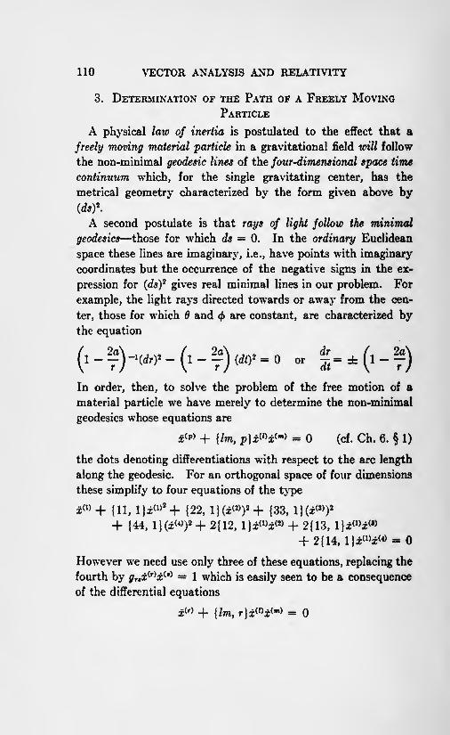
110 VECTOR ANALYSIS AND RELATIVITY
3. DETERMINATION OF THE PATH OF A FREELY MOVINGPARTICLE
A physical law of inertia is postulated to the effect that a
freely moving material particle in a gravitational field mil follow
the non-minimal geodesic lines of the four-dimensional space time
continuum which, for the single gravitating center, has the
metrical geometry characterized by the form given above by
A second postulate is that rays of light follow the minimal
geodesies those for which ds = 0. In the ordinary Euclidean
space these lines are imaginary, i.e., have points with imaginary
coordinates but the occurrence of the negative signs in the ex-
pression for (ds)* gives real minimal lines in our problem. For
example, the light rays directed towards or away from the cen-
ter, those for which 6 and < are constant, are characterized bythe equation
.(,.5)^., or j-In order, then, to solve the problem of the free motion of a
material particle we have merely to determine the non-minimal
geodesies whose equations are
x(f) + {lm, p}xwx(m) =
(cf. Ch. 6. 1)
the dots denoting differentiations with respect to the arc length
along the geodesic. For an orthogonal space of four dimensions
these simplify to four equations of the type
x (1) + {11, l}z<1)2 + {22, l}(z<) + {33, l}(z
(8))z
+ {44, l}(z>)* + 2{12, 1 }*>*< + 2(13, l)z(1)z<8)
+ 2{14, l}z(1)z> =
However we need use only three of these equations, replacing the
fourth by gr x(r)x(t) = 1 which is easily seen to be a consequence
of the differential equations
z(r> + {lm, rJzWxO-o =

PROBLEMS IN RELATIVITY 111
(if we multiply these by r and use r as an umbral symbol to
obtain
and then avail ourselves of the definition of the symbols
[lm, s]. (Ch. 6, 1.) j- (grtXrXs) is found to be zero). In our
problem it is convenient to omit the first of the four equations,
the other three simplifying, on using the values for the three-
index symbols given (Ch. 7, 2), to
* 1_ /,v 2 ^0J , J[_d02 .a _ n ,,,
202 vv 02 C/7"
where 0i= ( 1 ) ;
02=
7-2;
03= r
2sin
26;
To these we have to add the first integral
gii* + g*P + gw* + g*i*= 1 (D)
Equations (5) and (C) are immediately integrable giving
gzb constant = h say (B1
)
and
gd = constant = + C say
or on substituting the values of gz and 4
r2 sin2 0^ = h; (l-~\i-C
Equation (^4) may be written
(r2^ - r
2sin cos ^(<^
2 =
We now proceed to eliminate the parameter s and find a relation
connecting 6 and 0. Assuming that < 4s (0 = constant is a
special case which is susceptible to the analysis given below on a

112 VECTOR ANALYSIS AND RELATIVITY
mere interchange of and tp) we have
6-
so that
On substituting the value of </> from (B) we have
j
={2rr'6' + rtf"}^
2 - r20' -
r'<2 + 2 cot 00'<
2
where we denote differentiations with respect to the new inde-
pendent variable <f> by primes. Equating this to r2 sin 8 cos 0(<)2
and dividing out by r2^2 we obtain
0" - 2 cot 0(0')2 = sin 6 cos
If now we choose our directional coordinate so that initially
We see that 0" = and then on differentiating the above equa-
tion with respect to <f>, B'" = and so for all the other derivatives,
i.e., is a constant as <f> varies. Otherwise expressed the general
integral of the equation for as a function of <p is found by
writing z = cot yielding 2" + z = to be cot = L cos (<f> -f M)where L and M are arbitrary constants. We choose our initial
1P
conditions as above so that L = giving = -. Putting in this
value for we find
1*4 =h (BO
(0")\ r /
and from (D)

PROBLEMS IN RELATIVITY 113
Just as in the usual Newtonian treatment of planetary motion,
it is convenient to write r = l/u and to again use <p as the
independent variable. We have
r = u/uz =
u'<j>[u?= hu' (from J3')
and then (Z)') yields, on making use of (C"),
nz 1 Onu(u'Y + <u? = 2au* + g- + -- ()
Now, in the Newtonian treatment, the equation giving the path
of a particle under a central force is
u" + u = F/tfu?
where F is the acceleration towards the center and h=rz -dt
is the constant of areas. Instead of this we have on differen-
tiating the equation (E) just obtained
u" + u = 3auz + ?L
/r
so that we may, in a general manner, express Einstein's modifica-
tion of the Newtonian law of gravitation by saying that there is
superimposed to the inverse square law attraction an inverse
fourth power attraction, the relative strength of the attracting
masses being as 1 : 3hz. It remains to determine, at any rate
approximately, the nature and magnitude of the constants a, h
and C which arose in the integration of our differential equations.
For large values of r, and therefore small values of u, the New-
tonian law is a first approximation and so neglecting the term in
uz in the equation for u", a = F/uz =
jura; ju being the gravita-
tional constant and m the mass of the sun. Hence if we choose
our unit of mass so that n=l,a = m, where now m is what is known
as the gravitational mass of the attracting center (notice that we
have identified, for small values of u, our r and < with the usual
polar coordinates of Euclidean geometry). The velocity of light
directly towards the attracting center is 1 and accordinglyf

114 VECTOR ANALYSIS AND RELATIVITY
our unit of time is such that for small values of u the velocity of
light is unity; i.e., if the unit of length be 1 cm., the unit of
time employed is 1/c seconds where c = 3.1010. In the theory
of relativity there is no absolute distinction between space and
time and so we refer to our time unit as one centimeter (1 cm.
being the distance traversed by light in one time unit). It is
to be observed that in Newtonian mechanics gravitational mass
m has dimensions L*T~Z so that if L and T have the same dimen-
sions a = m has the dimensions of a length. The equation
n im"+- p
of the Newtonian theory yields
u -jz= P cos (<f>
-)
where P and fa are arbitrary constants of integration.
Comparing this with the polar equation of a conic
lu = \-\-e cos <t> (I= semi-latus rectum, e = eccentricity)
h*we have = I = A(l e-) where A is the semi-major axis.
mIf T is the period of revolution
2 X
whencem = W{A(\ - r) =
where o> is the angular velocity of the planet. This gives for the
sun m = 1.47 kilometers or 1.47.106 cms. For the planets then
m/r is a small quantity of the order 10~*. In order to determine
the constant C we differentiate
m ,- ...
u =rj (1 + e cos 0)
and find
(') + if =j(l + 2e cos* + e
2)=?gu
-g(l
-**)

PROBLEMS IN RELATIVITY 115
and comparing this with the equation (E) we have
It is to be observed that the values of m, C and h obtained in
this way are found from the Newtonian theory and so are to be
regarded as first approximations. In particular we have iden-
tified the h of (J3') with r2-j- so that we have written -^ -^at ds at
Accurately
(fromC")ds dt ds dt
ButMz
= d- -V\ A/
so that neglecting quantities of the order 10~8
d<p d<p
ds dt
Substituting the expressions just obtained in (E) we have to
integrate the first order differential equation
f^Y = 2mu* -u?+ 2mu/h*- m2
(l-
This equation defines u as an elliptic function of <f>; or inversely
<f> as an elliptic integral. It simplifies the algebra somewhat to
write mu v and to put ra2/A
2 = a. We have already seen
that ra2/F = -- so that if e is not very nearly equal to
unity a is a small quantity of the same order of magnitude as m/Aor 10~8
. Our equation is now
(//7)\
2M = 2tf -
Now the discriminant of the literal cubic
tti*2 + O2 + 3
=

116 VECTOR ANALYSIS AND RELATIVITY
is
4ai3a3 27a 2a3
2
For the cubic on the right-hand side of the equation giving (dv/d<fi)*
this is
8o3(l- Oe2)
-108a<(l
- e2)2.
On account of the small magnitude of a this is positive, the first
term being the dominant one. Hence the cubic has three real
roots which we denote, in descending order of magnitude, byi, tfc, *> When a = the roots are , 0, 0, and so we try first
= ka and find k = (1 e) or (1 + e) and then secondly
i + fra and find k = 2. Hence, to a first approximation,
the three roots of the cubic giving (dv/dpy are t>3= a(l e);
t = a(l + ); t>i= ^ 2a. Further since (dv/d<f>)* cannot be
negative in the problem t must lie between t>3 and 0j or between
d and + oo . As r does not tend to zero v does not tend to oo
and hence t> lies between Vt and 0j. We have
"I*/, dv
The variable t> oscillates between the values r3 and t>j; at these
values dv(d<f>= 0, so that v has an extreme value; as v passes
through the value t>j retracing its values both dv and the radical
change signs so that <f> steadily increases. The change in <p
between two successive extreme values of v, i.e., between peri-
helion and aphelion of the planet, is
p dt&<f>= I
Jn
It is convenient to make a simple linear transformation of the
variable of integration. Write v = a + 62 and determine the
coefficients a and 6 of the transformation so that to the roots r
and 2 of the cubic will correspond values and 1 of 2 respectively.
The values are a = r3 ;6 = vt vt and then the third root v\

PROBLEMS IN RELATIVITY 117
goes over into 2 = ^ where k2 = - - The cubic 2(v Vi)
(v Vz)(v vz) transforms into 2632(1 2) [j-2 2)
so that
k C1 dz
This simplifies considerably on writing 2 = sin2 6 when in fact
2k C'12 d6
Nowjo 02 ^3 2ae
(to a first approximation) is a small quantity of the same order
of magnitude as a; hence we can expand (1 kz sin20)~
1/2 in a
rapidly convergent series and a mere integration of the initial
terms will give a very good approximation to A<p. The multiplier
of the integral is
2 = x2M - =2[1
- 2a(3-
e)]'1 /2 =
2[1 + a(3-
e)]
and using J*'
/2sin
26 d8 = x/4 we find
but F = 4ae to a first approximation so
A?> = 7r{l + a(3 -e)}{! + ae] =
Hence in a complete revolution the perihelion advances by an
amount equal to
mz_ 3m
6<X 6 -rr-- - e2) r2
(l- e
2)
of a complete revolution, T being the period in our units. If we

118 VECTOR ANALYSIS AND RELATIVITY
wish to use the period in seconds and measure A in kilometers
then the unit of time in the formula given is the time it takes
light to travel 1 kilometer = 1/3.105seconds; hence if T is the
period in seconds the fractional advance of the perihelion per
revolution is, ftin<M/ ,-
57 On substituting the values of9.10 1 (1 (,)
A, T, and e for Mercury's path this works out to be an advance
of 43" per century. For the other planets e is much smaller than
for Mercury and the amount of advance of perihelion is much
smaller; save in the case of Mars the predicted advance is too
small to be detected by observation.
4. THE PATH OF A LIGHT RAY IN THE GRAVITATIONAL FIELD
OF A SINGLE ATTRACTING CENTER
These paths satisfy the equation (ds)2 = or ds = 0; they
are geodesies since, ds being the non-negative root of the expres-
sion for (ds)2, no curve can have a negative length. The method
of the preceding paragraph does not, however, immediately
apply since the arc length along a light ray, being a constant,
cannot be used as an independent variable or parameter in terms
of which the coordinates x may be expressed. Further in the
discussion of Oh. 6, 1, it was assumed that the integral
could be expanded in a Taylor series in powers of a so that the
existence of the derivative (d//da)a=, was presupposed. It is
apparent, however, on differentiation of
ds = ^gtmdx (l)dx(m) (I, m umbral)
a
that if ds = when a =0, (ds) becomes meaningless whenda
a on account of the zero factor (cfo)._o which occurs in the
denominator. These difficulties are overcome in the following
manner. If we investigate those curves (non-minimal) for which

PROBELMS IN RELATIVITY 119
the first variation of the integral I = J*(ds)~* is zero we are led
to exactly the same differential equations as those of Ch. 6, 1,
which express the fact that the first variation of / = fds is zero.
Accordingly we now derive the equations of the minimal geodesies
from the fact that the first variation of I = S(ds)z
is zero, ds
being zero along the curves. The coordinates x are supposed
expressed in terms of any convenient parameter v and differentia-
tions with respect to this parameter are denoted by primes.
The Euler-Lagrangian equations are (cf. Ch. 6, 1)
dF__
d ( dF \ _I
~i
I \T if' ' '
t *)
F = (fo)=
glmx^'x^' (I, m umbral)
= 2 (gr ix(l)t
) (I, m umbral)
= 2
or
_(!)" | f]m .1^.(/)'/-(m)' A (1 tnt ifm\\f.-i}\ffrix ~T~ [iTiit
f T\X c \i) m uiiiorai,/
Multiplying by g1" and using r as an umbral symbol we obtain
z<*>" + {lm, p}x^'x^' = (p=
1, 2, 3, 4)
which are exactly the equations of Ch. 6, 1. The first integral
of these equations which has already been mentioned may be
very briefly obtained as follows. Since F = gimx(l) 'x(m)
'
is
* Attention should, however, be called to the fact that this integral is not,
properly speaking, a line integral at all; its value depends not only on the
curve over which it is extended but on the particular parametric mode of
representation chosen for this curve. In order that the value of the integral
should not be dependent on the parametric representation the integrand should
be positively homogeneous of degree unity in the derivatives z'.

120 VECTOR ANALYSIS AND RELATIVITY
homogeneous of degree 2 in the x' we have, by Eider's theorem
on homogeneous functions,
a result immediately verifiable directly (r umbral). On multiply-
ing the equations
by x(r)/ and using r as an umbral symbol we obtain
(r), dF d f (r)
, dF \, dF(r)
/,
x{r>I x(r) -
I H 1x(T> =
oc uD V dx / doc
or
^_2^=0r/r '/r
showing that F is constant along the geodesies. The constant
is now zero instead of unity as it was in the case of the non-
minimal geodesies.
Before proceeding to calculate the deflection of the light rays
it will be well to prove an often quoted property of them. In a
statical gravitational field the time coordinate z (4) does not enter
into F = (d*)2
. Hence
d f dF \ dFI 1=0 or
\. 1
Vor -
.= const.
If, now, in the discussion of Ch. 6, 1, instead of keeping both
ends of the"
varied curve"C(a) fixed, we had allowed the ends
to vary also, the part of 81 which came outside the sign of integra-
tion when we integrated by parts would not vanish automatically.
Since the first variation is to vanish when the end points are
fixed as well as when they vary the part under the sign of integra-
tion vanishes as before yielding the Eulerian equations but in

PROBLEMS IN RELATIVITY 121
addition we have the end condition
2 "
=(r umbral)f
d*'
If now all the coordinates but z (4) are kept fixed
ait
and we find since- . is constant over the extremal curve'
dF|=o or 5/iW =
and as
dF
we have= o
which is known as the Fermat or Huyghens' Principle of Least
Time. It is an immediate consequence of the absence of xw
from (<fo)2
;there is a similar theorem for the symmetrical
attracting center:
= o
but this has no special utility. The Fermat Principle states that,
given two fixed points in space (by fixed is meant that the three
space coordinates for an observer attached to the gravitating
center are constant), a light signal passes from one to the other
in such a way that the first variation of the time interval is a
minimum.
With the same notation as that employed in 3 we find
g*v'= h; git'
- C
where h and C are constants and we find exactly as before that a
proper choice of our initial conditions for 6 enables us to

122 VECTOR ANALYSIS AND RELATIVITY
write 6 = r/2. The only difference is that (Z)') is replaced by
(1-
2m/r)-1(r')
8 + rV)2 -(1- 2m/r)(O
2 =
whence on writing r = l/u and using rV' = A we find
"A8
In order to get an idea of the order of magnitude of the constants
C, h of integration we make a first trial-approximation. The
largest value that u can have is IfR where R, the radius of the
sun, = 697,000, the units being kilometers. Hence we neglect,
for the moment, the u3 term in comparison with the others and
find at once
u = sin (<p <po)h
where ^o is a constant of integration. Hence Cfh is the largest
value of u and is therefore a small quantity of the order 1/106
.
Denoting this small quantity by a (a is the positive square root
of CVA2) we have
The discriminant (cf. Ch. 7, 3) of the cubic on the right is
4o2(l 27m2a2
), a positive quantity, so that the three roots are
real. When a = they reduce to l/2m, 0, 0, so that trying in
turn ka and (l/2m) -H ka we find the first approximation to the
three roots u9= a, v* = a, Ui = l/2m where we have ar-
ranged the roots so that u% < Wj < u\. For a second approxi-
mation, we try in turn a + fco2, a + kc?, (l/2m) -f kc? for
W|, ut, Ui respectively and find
w8= a + wio2 ; ut = a + mo?; u\ = (l/2m) 2mot2 .
We now, as before, determine a linear transformation which
sends u u3 into z = 0; u = u* into z = 1. It is u = a -f- bz

PROBLEMS IN RELATIVITY 123
where =2/3, b = uz w3 and then the third root uu\
goes into z = 1/fc2 where
Now the cubic 2mu3 w2-f- a2 cannot be negative in our problem
nor can u itself. At remote distances from the sun u - so
that initially u = and it increases to u = uz at which point u
has a maximum value, since ( -y- )= there. Then M- begins to
\d<pj_decrease and the radical V2wm3 if + 2 in the expression for
d(f>
, du
a2
also changes sign so that d<p keeps its sign. The angle < between
a point at a remote distance and the perihelion of the light ray
is given by the integral I,.
The excess ofJo V2mw3 - w2 + a2
twice this over TT is the deflection D experienced by the ray.
Hencedu=2 r
Jo9 I 9u H- or
which on writing u = a-\- bz becomes
dz
">(HOn making the final substitution 2 = sin
2 6 this becomes
d0njD -f 7T = _J_!9_ Vl - fc
2sin2
V , M,
Now= 4ma -\- higher powers in a
--f- a
2m

124 VECTOR ANALYSIS AND RELATIVITY
so that, m being 1.47, k2 is a small quantity of the same order
as a. Hence (1 A^ sin2 0)~1/2 can be expanded in a rapidly
convergent series and an integration of the initial terms of this
series gives a high approximation to D + TT. On substituting
the values of k and 6 the multiplier of the integral becomes
= 4(1 -f 2roa)-1/2 = 4(1
- ma)
whilst the lower limit of the integral is
. _, /I ma ._,!,, i v
sin 1
^ = sm l
-^ (1-- ma)
Here it is necessary to use the second approximation since u^ is
to be divided by w3 M? itself a small quantity of the first order.
On expanding
by Taylor's theorem we have for the lower limit (ir/4) \maso that
D + T = 4(1- m
In the term multiplied by
it is sufficient to take the rough approximation r/4 to the lower
limit and we have
gvngD = 4ma
a, in this expression, is the maximum value v* of u (to a first

PROBLEMS IN RELATIVITY 125
approximation), i.e., is the reciprocal of the radius of the sun.
An idea as to the closeness of this approximation is obtained
by using the second approximation
=U2 = a + mo?
R
The positive root a of this quadratic is
so that writing a = l/R is equivalent to neglecting m/R in
comparison with unity or to a neglect of 1 part in 5.105 . On
substituting m =1.47, R = 697,000 in the expression D = 4m/R
and converting this radian measure into seconds of arc we find
the value 1.73" predicted by Einstein for a light ray which just
grazes the sun.*
*For a fuller discussion of the problems dealt with in this chapter reference
is made to two papers by the author in the Phil. Mag. of dates Jan. (1922)
and March (1922) respectively. For an alternative treatment of the subject
matter of 2 the reader should consult the paper Concomitants of Quadratic
Differential Forms by A. R. Forsyth in the Proc. Roy. Soc. Edin. May (1922) .


CMO
0)
,)H -P
vO HCO H
03
O >>
hfe
bD 0)
03 >
University of Toronto
Library
DO NOT
REMOVE
THE
CARD
FROM
THIS
Acme Library Card Pocket
LOWE-MARTIN CO. LIMITED