Vector Analysis in a Nutshell

by Vitaly Vanchurin1

December 11, 2014

1If you have comments or error corrections, please send them to the LYX Doc-

umentation mailing list: lyx-docs@lists.lyx.org

Contents

0.1 Vectors . . . . . . . . . . . . . . . . . . . . . . . . . . . . . . . 10.2 Components . . . . . . . . . . . . . . . . . . . . . . . . . . . . 20.3 Gradient . . . . . . . . . . . . . . . . . . . . . . . . . . . . . 40.4 Divergence and Curl . . . . . . . . . . . . . . . . . . . . . . . 50.5 Integrals . . . . . . . . . . . . . . . . . . . . . . . . . . . . . . 80.6 Exact differentials . . . . . . . . . . . . . . . . . . . . . . . . . 100.7 Generalized functions . . . . . . . . . . . . . . . . . . . . . . . 130.8 Simple transformations . . . . . . . . . . . . . . . . . . . . . . 130.9 General transformations . . . . . . . . . . . . . . . . . . . . . 16

i

CONTENTS 1

0.1 Vectors

Vector quantities (or three-vectors) are denoted by boldface letters A,B, ...in contrast to scalar quantities denoted by ordinary letters A,B, .... Forexample, in Cartesian coordinates a vector

A = (Ax, Ay, Az) (1)

has a length (or magnitude)

A ≡ |A| =√

A2x + A2

y + A2z (2)

which is a scalar. Scalars are real numbers or elements in space R and vectorsare elements in space R

3. For vectors A,B, ... ∈ R3 and angle θ between A

and B one can define:

1. Addition:A+B ≡ (Ax +Bx, Ay +By, Az +Bz) (3)

which is commutativeA+B = B+A (4)

associative(A+B) +C = A+ (B+C) (5)

and defines inverse (or minus) vector

A+ (−A) ≡ 0 (6)

where the zero vector is0 ≡ (0, 0, 0). (7)

Geometrically the addition is understood by parallel transporting vec-tor B so that it starts where the vector A ends. Then the vector A+B

points from the beginning of vector A to the end of vector B.

2. Multiplication by scalar:

aA ≡ (aAx, aAy, aAz) (8)

which is distributive

a (A+B) = aA+ aB (9)

where a ∈ R is the scalar.Geometrically the resulting vector aA is a vector pointing in the samedirection (or in the opposite direction if a < 0) as vector A but whosemagnitude is a times larger (or smaller if |a| < 1).

CONTENTS 2

3. Dot product (or scalar product):

A ·B ≡ AB cos θ (10)

which is commutativeA ·B =B ·A (11)

and distributive

A · (B+C) = A ·B+A ·C. (12)

Geometrically the dot product measures the length of the vector A

when projected to the direction of B times B or equivalently the lengthof the vector B when projected to the direction of A times A.

4. Cross product (or vector product):

A×B ≡ AB sin θn (13)

where the vector n has unit length (unit vector)

|n| = 1 (14)

which is non-commutative (or anti-commutative)

A×B =−B×A (15)

and distributive

A× (B+C) = A×B+A×C. (16)

Geometrically the magnitude of vector A ×B is the area of parallelo-gram generated by A and B and points in the direction n perpendicularboth A and B using the right-hand-rule (just a convention). Notethat the cross product exist only in three and seven dimensional spaces.

0.2 Components

It is convenient to write vectors in the components form

A = (Ax, Ay, Az) = Axx + Ayy + Azz (17)

where x, y and z are unit vectors in the direction of positive x, y and z axes.Then,

CONTENTS 3

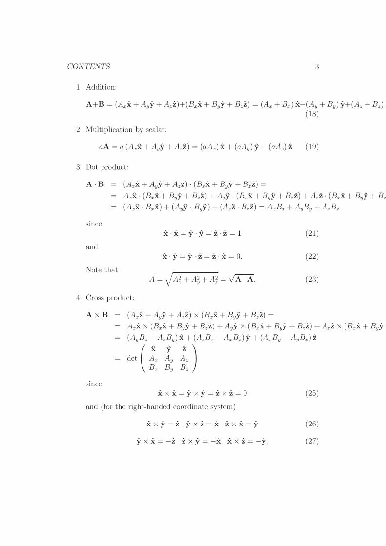
1. Addition:

A+B = (Axx+ Ayy + Azz)+(Bxx+Byy +Bzz) = (Ax +Bx) x+(Ay +By) y+(Az +Bz) z(18)

2. Multiplication by scalar:

aA = a (Axx + Ayy + Azz) = (aAx) x+ (aAy) y + (aAz) z (19)

3. Dot product:

A ·B = (Axx + Ayy + Azz) · (Bxx+Byy +Bzz) =

= Axx · (Bxx +Byy +Bzz) + Ayy · (Bxx+Byy +Bzz) + Azz · (Bxx+Byy +Bzz

= (Axx ·Bxx) + (Ayy · Byy) + (Azz · Bzz) = AxBx + AyBy + AzBz

sincex · x = y · y = z · z = 1 (21)

andx · y = y · z = z · x = 0. (22)

Note thatA =

√

A2x + A2

y + A2z =

√A ·A. (23)

4. Cross product:

A×B = (Axx+ Ayy + Azz)× (Bxx +Byy +Bzz) =

= Axx× (Bxx+Byy +Bzz) + Ayy × (Bxx +Byy +Bzz) + Azz× (Bxx +Byy +

= (AyBz −AzBy) x + (AzBx −AxBz) y + (AxBy − AyBx) z

= det

x y z

Ax Ay Az

Bx By Bz

sincex× x = y × y = z× z = 0 (25)

and (for the right-handed coordinate system)

x× y = z y × z = x z× x = y (26)

y × x = −z z× y = −x x× z = −y. (27)

CONTENTS 4

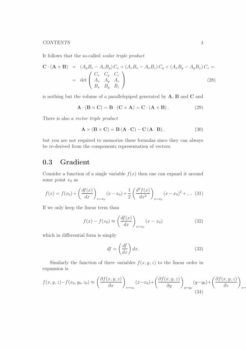
It follows that the so-called scalar triple product

C · (A×B) = (AyBz −AzBy)Cx + (AzBx − AxBz)Cy + (AxBy − AyBx)Cz =

= det

Cx Cy Cz

Ax Ay Az

Bx By Bz

(28)

is nothing but the volume of a parallelepiped generated by A, B and C and

A · (B×C) = B · (C×A) = C · (A×B) . (29)

There is also a vector triple product

A× (B×C) = B (A ·C)−C (A ·B) , (30)

but you are not required to memorize these formulas since they can alwaysbe re-derived from the components representation of vectors.

0.3 Gradient

Consider a function of a single variable f(x) then one can expand it aroundsome point x0 as

f(x) = f(x0)+

(

df(x)

dx

)

x=x0

(x−x0)+1

2

(

d2f(x)

dx2

)

x=x0

(x−x0)2+ .... (31)

If we only keep the linear term than

f(x)− f(x0) ≈(

df(x)

dx

)

x=x0

(x− x0) (32)

which in differential form is simply

df =

(

df

dx

)

dx. (33)

Similarly the function of three variables f(x, y, z) to the linear order inexpansion is

f(x, y, z)−f(x0, y0, z0) ≈(

∂f(x, y, z)

∂x

)

x=x0

(x−x0)+

(

∂f(x, y, z)

∂y

)

y=y0

(y−y0)+

(

∂f(x, y, z)

∂z

)

x=x

(34)

CONTENTS 5

or in differential form

df =

(

∂f

∂x

)

dx+

(

∂f

∂y

)

dy +

(

∂f

∂z

)

dz. (35)

This can also be rewritten as a dot product of two vectors

df =

((

∂f

∂x

)

x +

(

∂f

∂y

)

y +

(

∂f

∂z

)

z

)

· (dxx + dyy+ dzz)

=

(

∂f

∂x,∂f

∂y,∂f

∂z

)

· (dx, dy, dz)

=

((

∂...

∂x,∂...

∂y,∂...

∂z

)

f

)

· (dx, dy, dz). (36)

where in the last line a vector-like operator acts on the function f to producea vector. The vector is called a gradient of f defined as

∇f =

(

∂f

∂x,∂f

∂y,∂f

∂z

)

=

(

∂f

∂x

)

x+

(

∂f

∂y

)

y +

(

∂f

∂z

)

z. (37)

Geometrically gradient ∇f is a vector pointing in the direction of (a local)maximum increase of function f and its magnitude gives the rate of the in-crease. For instance at a local maxima, minima or saddle point, the gradientof a function is a zero vector.

It is also useful to define a vector-like operator known as del (or nabla)operator

∇ ≡(

∂...

∂x,∂...

∂y,∂...

∂z

)

. (38)

Then the gradients can be produced by acting with nabla on functions

∇f =

(

∂...

∂x,∂...

∂y,∂...

∂z

)

f =

(

∂f

∂x,∂f

∂y,∂f

∂z

)

(39)

where ∇ is treated as vector quantity and f is treated as scalar quantity.

0.4 Divergence and Curl

One can also imagine a vector function which has three values Ax(x′, y′, z′),

Ay(x′, y′, z′) and Az(x

′, y′, z′) in each point in space or equivalently thereis a three-component vector v(x′, y′, z′) attached to each point (x′, y′, z′).Mathematically speaking vectors are elements of a tangent space at a given

CONTENTS 6

point (x′, y′, z′) ∈ T(x′,y′,z′)M on a manifold (in our case a 3 dimension Eu-clidean space M = R

3) and the vector fields are elements of a tangent bundlev ∈ TM. One can also think of the nabla operator as a vector field operatoralthough it is not usually called this way

∇ ≡(

[

∂...

∂x

]

(x′,y′,z′)

,

[

∂...

∂y

]

(x′,y′,z′)

,

[

∂...

∂z

]

(x′,y′,z′)

)

. (40)

(Take your time and think what it means). We shall omit writing (x′, y′, z′),but it is assumed that the scalar and vector quantities are fields.

Given scalar fields f, g, ... vector fields v,u, ... and a vector operator ∇ onecan do the usual vector manipulations at each point separately to producenew fields:

Addition:A+B = (Ax +Bx, Ay +By, Az +Bz) (41)

1. Multiplication by scalar:

aA = (aAx, aAy, aAz) (42)

or

∇a =

(

∂...

∂x,∂...

∂y,∂...

∂z

)

a =

(

∂a

∂x,∂a

∂y,∂a

∂z

)

(43)

which is a gradient of a scalar field a which is a vector field as we havealready mentioned.

2. Dot product (or scalar product):

A ·B = AxBx + AyBy + AzBz (44)

or

∇ ·A =

(

∂...

∂x,∂...

∂y,∂...

∂z

)

· (Ax, Ay, Az) = . (45)

which is a scalar field called divergence of a vector A. Geometricallythe divergence measures the amount by which the lines of vector fielddiverge from each other.

3. Cross product (or vector product):

A×B = det

x y z

Ax Ay Az

Bx By Bz

(46)

CONTENTS 7

or

∇×A = det

x y z∂...∂x

∂...∂y

∂...∂z

Ax Ay Az

. (47)

which is a vector field called curl of a vector A. Geometrically the curlmeasures the amount by which the lines of vector field curl around agiven point.

According to Helmholtz theorem the knowledge of divergence ∇ ·A and ofcurl ∇×A of some vector field A is sufficient to determine the vector fielditself (given that both ∇ ·A and ∇×A fall off faster than 1/r2 as r → ∞).

Using definitions of gradient 43, divergence 45 and curl 47 it is straight-forward to derive different product rules

∇(ab) = a∇b+ b∇a

∇(A ·B) = (A · ∇)B+ (B · ∇)A

∇ · (aA) = a∇ ·A+A · ∇a

∇ · (A×B) = B · (∇×A)−A · (∇×B)

∇× (aA) = a (∇×A)−A× (∇a)

∇× (A×B) = (B · ∇)A− (A · ∇)B+A (∇ ·B)−B (∇ ·A) (48)

and quotient rules

∇(a

b

)

=b∇a− a∇b

b2

∇ ·(

A

a

)

=a (∇ ·A)−A · (∇a)

a2

∇×(

A

a

)

=a (∇×A) +A× (∇a)

a2. (49)

From definitions one can also derive expressions for second derivatives themost useful of which is a Laplacian operator

∇2a ≡ ∇ · (∇a) . (50)

It is also extremely important to remember that the curl of gradient or adivergence of curl is always zero

∇× (∇a) = (0, 0, 0)

∇ · (∇×A) = 0. (51)

CONTENTS 8

0.5 Integrals

For a function of a single variable f(x) there is only one type of integral

∫ b

a

f(x)dx (52)

but for a function of three variables f(x, y, z) one can integrate over line (orpath) , over area (or surface) and over volume:

• Path integral∫

P

v(l) · dl (53)

where the integral is take over some path P from point l = a to pointl = b. (The subscript P is often dropped, but it is always implied thatthe integral is over some path.) For example, work required to move aparticle along some path is given by

W =

∫

F(l) · dl (54)

where F is a force acting on the particle.

• Surface integral∫

S

v(l) · da (55)

where the integral is take over some surface S (also often omitted sub-script) and da is an infinitesimal patch of area with direction perpen-dicular to the surface (lousy, but common notation) with also a signambiguity in the definition. For closed surfaces

∮

v(l) · da (56)

the convention is that the “infinitesimal area” vector points outwards.For example, consider a surface integral of

v(x, y, z) = 2xzx + (x+ 2)y + y(z2 − 3)z (57)

over a cubical box with side 2. Then there will be six contributions tothe integral

1. x = 2 and da = dydzx implies v · da = 2xzdydz = 4zdydz, and∫

v · da = 4

∫ 2

0

dy

∫ 2

0

zdz = 16. (58)

CONTENTS 9

2. x = 0 and da = −dydzx implies v · da = −2xzdydz = 0, and

∫

v · da = 0. (59)

3. y = 2 and da = dxdzy implies v · da = (x+ 2)dxdz, and

∫

v · da =

∫ 2

0

(x+ 2)dx

∫ 2

0

dz = 12. (60)

4. y = 0 and da = −dxdzy implies v · da = −(x+ 2)dxdz, and

∫

v · da = −∫ 2

0

(x+ 2)dx

∫ 2

0

dz = −12. (61)

5. z = 2 and da = dxdyz implies v · da = y(z2 − 3)dxdy = ydxdy, and

∫

v · da =

∫ 2

0

dx

∫ 2

0

ydy = 4. (62)

6. z = 0 and da = −dxdyz implies v · da = −y(z2 − 3)dxdy = 3ydxdy,and

∫

v · da = 3

∫ 2

0

dx

∫ 2

0

ydy = 12. (63)

And the total flux is∮

v · da = 16 + 0 + 12− 12 + 4 + 12 = 32. (64)

• Volume integral

∫

V

f dx3 =

∫

V

f(x, y, z)dxdydz (65)

which is nothing but a triple integral which can be taken in any order

∫(∫(∫

f(x, y, z)dx

)

dy

)

dz =

∫(∫(∫

f(x, y, z)dz

)

dx

)

dy = ...

(66)

CONTENTS 10

0.6 Exact differentials

The fundamental theorem describes how to integrate functions which areexact differentials. For example, if

F (x) =df(x)

dx(67)

then∫ x=b

x=a

F (x)dx = f(b)− f(a). (68)

In higher dimensions this results generalizes to integrating a function

F (x, y, z) = ∇f(x, y, z). (69)

over an arbitrary path

∫

b

a

(∇f) · dl = f(b)− f(a) (70)

connecting points a and b. For example, if the force in equation(54) isconservative (e.g. gravitational force, but not friction force)

F = −∇V (71)

then the work only depend on the value of the potential in the initial andfinal points

W =

∫

b

a

F(l) · dl = V (a)− V (b). (72)

and over closed paths the work is always zero

W =

∮

F(l) · dl = 0. (73)

Note that it is always possible to rewrite a curl-less vector fields as a gradient

∇× F = 0 ⇔ F = −∇V (74)

and thus the path independence of work (72) and vanishing of work for closedpaths (73) would follow automatically. And if the vector field is not curl-lesswe can still rewrite it as

∇× F 6= 0 ⇒ F = −∇V +∇×A.

CONTENTS 11

A straightforward generalization of the same idea leads to the Gauss’s (ordivergence) theorem

∫

V

(∇ · v) dx3 =

∮

S

v · da (75)

and to Stokes’s (or curl) theorem

∫

S

(∇× v) · da =

∮

P

v · dl. (76)

Roughly speaking the Gauss’s theorem (75) describes the two ways of cal-culate the number of (vector v) field lines entering a given volume minusthe number of field lines leaving the volume. On can calculate it either byintegrating divergence of the field lines over the volume (as on the left handside), or by integrating the flow of the field lines over the surface (as on theright hand side).

Similarly the Stokes’s theorem (76) describes the different ways howswirling of the field lines can be calculate. One can calculate it by inte-grating the curl of field lines over the area (as on the left hand side), or bythe integrating the rotation of field lines as we go around boundary (as onthe right hand side).

For a vector field (57)

v(x, y, z) = 2xzx + (x+ 2)y + y(z2 − 3)z (77)

we can find∇ · v = 2z + 2yz (78)

∇× v = det

x y z∂...∂x

∂...∂y

∂...∂z

2xz x+ 2 y(z2 − 3)

= (z2 − 3)x+ 2xy + z. (79)

It is now easy to check that

∫ 2

0

∫ 2

0

∫ 2

0

(2z + 2yz) dxdydz = 16 + 16 = 32 (80)

is the same as total flux through the boundary (64) as correctly predicted byGauss’s theorem (75). Moreover for the face of the cube (y = 0)

∫ 2

0

∫ 2

0

(

(z2 − 3)x+ y2x+ z)

· ydxdz =

∫ 2

0

∫ 2

0

2xdxdz = 8 (81)

CONTENTS 12

or∫

z=0

(2xzx · x) dx+

∫

x=2

(

y(z2 − 3)z · z)

dz +

+

∫

z=2

(2xzx · (−x)) dx+

∫

x=0

(

y(z2 − 3)z · (−z))

dz =

0 + 0 +

∫ 0

2

(4xx · (−x)) dx+ 0 =

∫ 2

0

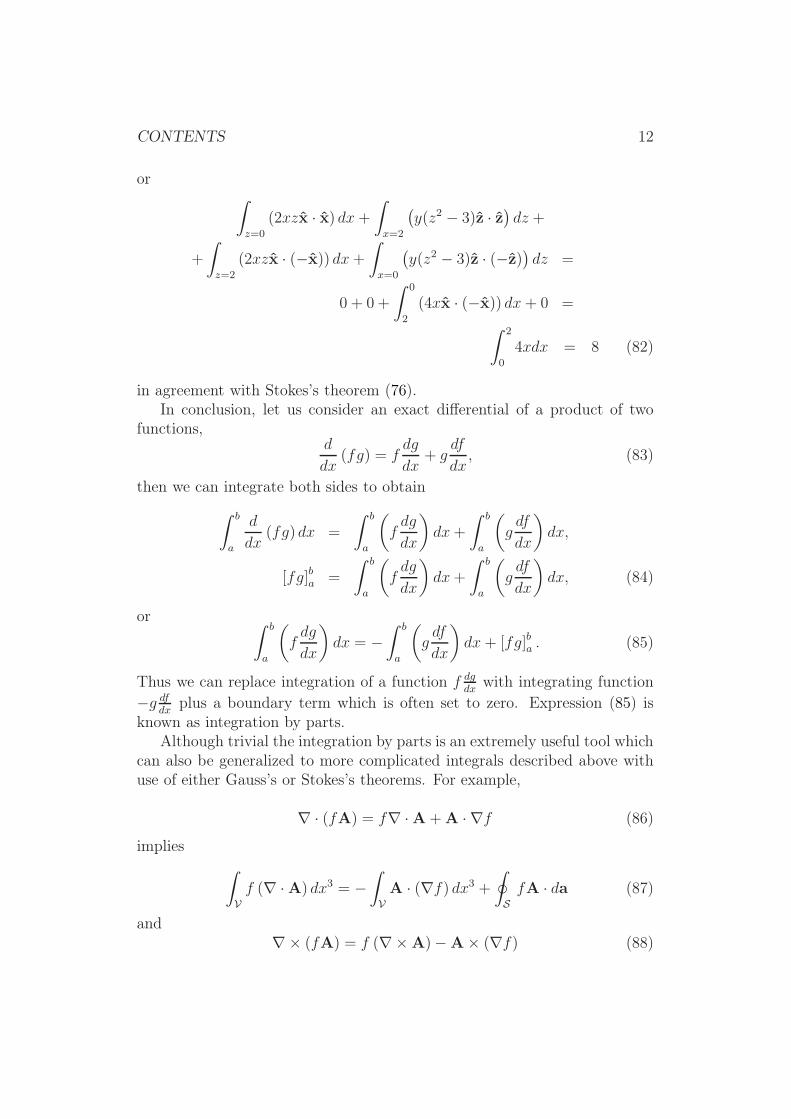
4xdx = 8 (82)

in agreement with Stokes’s theorem (76).In conclusion, let us consider an exact differential of a product of two

functions,d

dx(fg) = f

dg

dx+ g

df

dx, (83)

then we can integrate both sides to obtain

∫ b

a

d

dx(fg)dx =

∫ b

a

(

fdg

dx

)

dx+

∫ b

a

(

gdf

dx

)

dx,

[fg]ba =

∫ b

a

(

fdg

dx

)

dx+

∫ b

a

(

gdf

dx

)

dx, (84)

or∫ b

a

(

fdg

dx

)

dx = −∫ b

a

(

gdf

dx

)

dx+ [fg]ba . (85)

Thus we can replace integration of a function f dg

dxwith integrating function

−g df

dxplus a boundary term which is often set to zero. Expression (85) is

known as integration by parts.Although trivial the integration by parts is an extremely useful tool which

can also be generalized to more complicated integrals described above withuse of either Gauss’s or Stokes’s theorems. For example,

∇ · (fA) = f∇ ·A+A · ∇f (86)

implies

∫

V

f (∇ ·A) dx3 = −∫

V

A · (∇f) dx3 +

∮

S

fA · da (87)

and∇× (fA) = f (∇×A)−A× (∇f) (88)

CONTENTS 13

implies

∫

S

f (∇×A) · da = −∫

V

(A× (∇f)) · da+

∮

P

fA · dl. (89)

0.7 Generalized functions

There is a special class of functions known as generalized functions (or distri-bution functions). The most useful example of such function is the (Dirac)δ-function. Strictly speaking it is not a function as it only makes sense totalk about δ-function when it is inside of an integral. In one dimension itcan be defined by the following expression

∫

∞

−∞

δ(x− a)f(x)dx ≡ f(a) (90)

where f(x) is an arbitrary function.Sometimes it is convenient to expressδ-function as a derivative of the Heaviside step function, i.e.

δ(x) =d

dxH(x). (91)

In three dimensions it is defined as a product of three delta functions

δ(3) (r) = δ(x)δ(y)δ(z) (92)

so that∫

∞

−∞

∫

∞

−∞

∫

∞

−∞

δ(x− a)δ(y − b)δ(z − c)f(x, y, z)dxdydz = f(a, b, c) (93)

or∫

f(r)δ(r − a)dx3 = f(a). (94)

One can think of δ-function as a probability distribution for a point particlelocated at a since the integral of the entire space is exactly one

∫

∞

−∞

δ(3)(r− a)dx3 = 1. (95)

0.8 Simple transformations

Clearly the choice of the reference frame or coordinates system (i.e. origin,axes, handedness, etc ) is arbitrary, and we want the laws of physics not

CONTENTS 14

to depend on this choice. In other words if we make predictions of how agiven system should behave in one coordinate system then we should havea rule how to make predictions in another coordinate system. For that weneed a rule how to transform different quantities from one system to another.In fact all of the quantities (such as scalars, vectors, tensors, spinors, etc)are distinguished from other by the way they transform under changes ofcoordinates.

What are the possible transformations in Euclidean three dimensionalspace (denoted by 3D)? There are:

• 3 translations (or shifts) along x, y and z directions

• 3 rotations from x to y, from y to z and from z to x.

These are linearly independent transformations (i.e. there are no non-zerolinear combinations of these six transformations which leaves the system un-transformed), but one can produce other linearly dependent transformationsby forming linear combinations of these six transformations (e.g. shift by -5meters along y, rotate by π/5 from z to x and then rotate by π/7 from x toy). How many linearly independent transformations in 1D? 2D? 4D? nD?In n dimensions there are n translations and as rotation many rotations asthere are distinct pairs of axis (rotations from x to y, from x toz, etc.)

(n− 1) + (n− 2) + .... + 2 + 1 =n(n− 1)

2.

Thus there are

n+n(n− 1)

2=

n(n+ 1)

2

independent transformations.Linear combination of translations can be described by a translation vec-

torT = (Tx, Ty, Tz) (96)

of the old coordinate system (x, y, z) to new coordinate system (x′, y′, z′).Note that the translation vector is also expressed in the old (unprimed)coordinates. Then scalars (e.g. A) and vectors (e.g. A = (Ax, Ay, Az))transforms into A′ and A′ = (A′

x′, A′

y′ , A′

z′) such that

A′ = A (97)

and

A′ = A. (98)

CONTENTS 15

This is just a statement of the fact that vectors parallel transported in theEuclidean space do not change.

For brevity of notations (and to confuse readers) the primes are oftendropped either for the newly transformed vector (as in books on generalrelativity) or for the new coordinates (as in book on electrodynamics) sothat

A′

x = Ax

A′

y = Ay

A′

z = Az (99)

The notations are confusing, but it should always be clear from the contextwhether we are in the old (unprimed) or in the new (primed) coordinatessystem.

Linear combination of rotations can be described by a rotation matrix

Rxx Rxy Rxz

Ryx Ryy Ryz

Rzx Rzy Rzz

≡ (100)

cosφ1 sin φ1 0− sin φ1 cosφ1 0

0 0 1

+

1 0 00 cosφ2 sinφ2

0 − sinφ2 cosφ2

+

cos φ3 0 − sinφ3

0 1 0sinφ3 0 cos φ3

.

for some angles φ1, φ2 and φ3. Then scalars and vector transform as

A′ = A (101)

A′

i =

3∑

j=1

RijAj (102)

where it is assumed that i = 1, 2, 3 and it stands correspondently for ei-ther x, y, z. or using the Einstein summation convention (always sum overrepeated indices)

A′

i = RijAj. (103)

For more complicated objects such as tensors the transformation law wouldbe written as

M ′

ij =

3∑

k,l=1

RikRjlMkl (104)

or (with Einstein summation convention) simply

M ′

ij = RikRjlMkl. (105)

CONTENTS 16

Clearly, the simplest transformation rule is for scalar quantities - they do notchange under coordinate transformations.

0.9 General transformations

So far we had been using Cartesian coordinates, but nothing can stop usfrom describing the points on different manifolds using other coordinatessystem. The two most useful examples are the so-called spherical and cylin-drical coordinates both of which are generalizations of two dimensional polarcoordinates to our three dimensional space:

• Spherical coordinates

x = r sin θ cosφ

y = r sin θ sinφ

z = r cos θ (106)

where r ∈ (0,∞) is the radial distance,θ ∈ (0, π) is the inclination angleand φ ∈ [0, 2π) is azimuthal angle.

• Cylindrical coordinates

x = s cosφ

y = s sinφ

z = z (107)

where s ∈ (0,∞) is the radial direction projected to x − y plane andφ ∈ [0, 2π) is the same azimuthal angle as in spherical coordinates.

Then any vector in Cartesian coordinates (x, y, z)

A = Axx+ Ayy + Azz (108)

can be expressed in terms of the new coordinates (r, θ, φ)

A = Arr+ Aθθ + Aφφ (109)

or (s, φ, z)A = Arr+ Aφφ+ Azz (110)

and vise versa. The transformation matrix is called Jacobian an can becalculated for any transformation.

For example, using the inverse Jacobian matrix

CONTENTS 17

J−1 =

∂x∂r

∂x∂θ

∂x∂φ

∂y

∂r

∂y

∂θ

∂y

∂φ∂z∂r

∂z∂θ

∂z∂φ

=

sin θ cosφ r cos θ cosφ −r sin θ sinφsin θ sinφ r cos θ sin φ r sin θ cos φ

cos θ −r sin θ 0

(111)one can expressed vectors in new coordinates

A ∝

100

, B ∝

010

, C ∝

001

(112)

in terms of old coordinates

J−1A ∝

sin θ cosφsin θ sin φ

cos θ

= sin θ cosφx+ sin θ sin φy + cos θz.

J−1B ∝

r cos θ cosφr cos θ sin φ−r sin θ

= r cos θ cosφx+ r cos θ sinφy − r sin θz.

J−1C ∝

−r sin θ sinφr sin θ cos φ

0

= −r sin θ sinφx+ r sin θ cos φy. (113)

which can be normalized to define

r ≡ cosφx+ sin θ sin φy + cos θz

θ ≡ cos θ cosφx+ cos θ sinφy − sin θz.

φ ≡ − sinφx+ cos φy. (114)

In fact these normalization constants (1, r and r sin θ) are important as theyappears in a general infinitesimal displacement

dl = drr+ rdθθ + r sin θdφφ (115)

often written in terms of the so-called metric tensor

dl2 = dr2 + rdθ2 + dφ2 =

1 0 00 r2 00 0 r2 sin2 θ

(116)

Similarly for cylindrical coordinates

x = s cosφ

y = s sinφ

z = z (117)

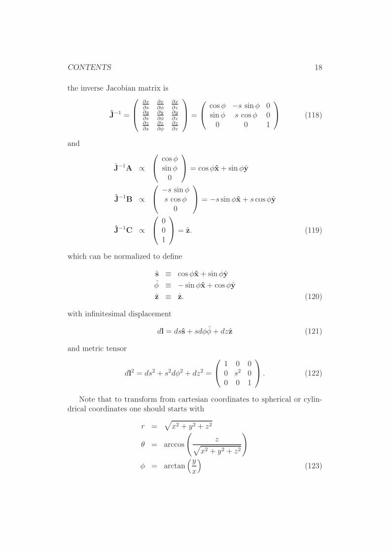
CONTENTS 18

the inverse Jacobian matrix is

J−1 =

∂x∂s

∂x∂φ

∂x∂z

∂y

∂s

∂y

∂φ

∂y

∂z∂z∂s

∂z∂φ

∂z∂z

=

cos φ −s sinφ 0sinφ s cosφ 00 0 1

(118)

and

J−1A ∝

cosφsinφ0

= cosφx+ sinφy

J−1B ∝

−s sin φs cosφ

0

= −s sin φx+ s cosφy

J−1C ∝

001

= z. (119)

which can be normalized to define

s ≡ cos φx+ sinφy

φ ≡ − sin φx+ cosφy

z ≡ z. (120)

with infinitesimal displacement

dl = dss+ sdφφ+ dzz (121)

and metric tensor

dl2 = ds2 + s2dφ2 + dz2 =

1 0 00 s2 00 0 1

. (122)

Note that to transform from cartesian coordinates to spherical or cylin-drical coordinates one should starts with

r =√

x2 + y2 + z2

θ = arccos

(

z√

x2 + y2 + z2

)

φ = arctan(y

x

)

(123)

CONTENTS 19

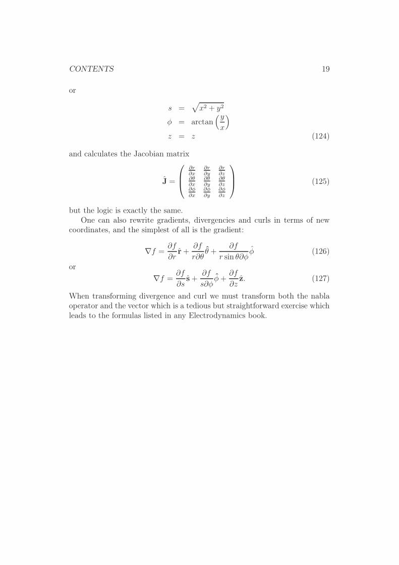
or

s =√

x2 + y2

φ = arctan(y

x

)

z = z (124)

and calculates the Jacobian matrix

J =

∂r∂x

∂r∂y

∂r∂z

∂θ∂x

∂θ∂y

∂θ∂z

∂φ

∂x

∂φ

∂y

∂φ

∂z

(125)

but the logic is exactly the same.One can also rewrite gradients, divergencies and curls in terms of new

coordinates, and the simplest of all is the gradient:

∇f =∂f

∂rr+

∂f

r∂θθ +

∂f

r sin θ∂φφ (126)

or

∇f =∂f

∂ss+

∂f

s∂φφ+

∂f

∂zz. (127)

When transforming divergence and curl we must transform both the nablaoperator and the vector which is a tedious but straightforward exercise whichleads to the formulas listed in any Electrodynamics book.