Embed Size (px)
Citation preview

VEGA Missionization and Post Flight Analyses
1
VEGA MISSIONIZATION AND
POST FLIGHT ANALYSES
PhD thesis
December 2009
Maurizio Bernard
Dottorato in tecnologia aeronautica e spaziale
XXII ciclo
Dipartimento di Ingegneria Aeronautica ed Astronautica
Docente guida: G. De Matteis
Coordinatore: R. Barboni

VEGA Missionization and Post Flight Analyses
2
ABSTRACT
This document is submitted for evaluation after the third year of PhD in aeronautics and space technologies. The PhD is a co-operation of the Department of Aeronautics and Astronautics Engineering (DIAA) of Sapienza University of Rome and ELV, prime contractor for development of the European space launcher VEGA.
The work was originally motivated by a research in the field of missionization, within program LYRA (funded by Italian Space Agency ASI to ELV), and eventually focused on Post Flight Analyses.
Besides analyses in the frame of VEGA design and qualification, research and application of non-linear techniques for systems identification has been carried out in the frame of a research program PRORA-USV, concerning re-entry space vehicles, in co-operation with CIRA, Italian Centre for Aerospace Research.
The work deals with systems engineering for launch systems (VEGA missionization), recursive real time estimation of wind on launch vehicle VEGA and non-linear systems identification in post flight analysis with recursive stochastic approach.
INDEX
Abstract ................................................................................................................................................ 2 Index..................................................................................................................................................... 2 1 Introduction .................................................................................................................................. 5
1.1 Executive summary .............................................................................................................. 5 1.2 Framework and objectives ................................................................................................... 7
1.2.1 VEGA program ................................................................................................................ 7 1.2.2 LYRA program ................................................................................................................ 8 1.2.3 PRORA-USV program .................................................................................................... 9 1.2.4 Objective of this study ................................................................................................... 10
1.3 Reference documents ......................................................................................................... 11 1.3.1 Reference documents ..................................................................................................... 12 1.3.2 Documents restricted to VEGA program or ELV property ........................................... 15 1.3.3 Documents property of CIRA ........................................................................................ 17
1.4 Acronyms, abbreviations, definitions ................................................................................ 18 1.5 List of figures, tables and equations ................................................................................... 19
1.5.1 List of figures ................................................................................................................. 20 1.5.2 List of tables ................................................................................................................... 23 1.5.3 List of equations ............................................................................................................. 23
2 VEGA Missionization ................................................................................................................ 26 2.1 The concept of missionization ........................................................................................... 26 2.2 Missionization plan ............................................................................................................ 27 2.3 Aspects within VEGA missionization ............................................................................... 30
2.3.1 Project management, planning and process control ....................................................... 30 2.3.2 Systems engineering ...................................................................................................... 31 2.3.3 Data Management .......................................................................................................... 32 2.3.4 Configuration Management ........................................................................................... 32

VEGA Missionization and Post Flight Analyses
3
2.3.5 Engineering Change Proposals (ECP) ........................................................................... 33 2.3.6 Documentation management .......................................................................................... 33
2.4 Systems Engineering data management in VEGA ............................................................ 34 2.4.1 Systems Engineering Database (SED) ........................................................................... 34 2.4.2 Data structure and format ............................................................................................... 35
2.5 Missionization Tool Prototype and SED2 ......................................................................... 37 3 Activities within VEGA design and missionization .................................................................. 39
3.1 Design validation process .................................................................................................. 39 3.1.1 Design parameters and general specifications ............................................................... 39 3.1.2 Dispersed trajectories for design [NT-168] ................................................................... 41
3.2 GNC analyses for PL loading ............................................................................................ 44 3.2.1 High level logic of systems engineering ........................................................................ 45 3.2.2 Executive summary of [NT-289] ................................................................................... 46 3.2.3 Local acceleration for loading ........................................................................................ 47 3.2.4 Sizing criterion based on LV and PL input data ............................................................ 48 3.2.5 Bending modes processing............................................................................................. 51 3.2.6 General results................................................................................................................ 52 3.2.7 Closed loop bending amplification ................................................................................ 55 3.2.8 GNC recovery for amplification at tail-off .................................................................... 58
3.3 TVC SWIL impacts and identification .............................................................................. 59 3.3.1 Motivation, framework and objectives .......................................................................... 59 3.3.2 Analyses on P80 TVC SWIL model [NT-113] .............................................................. 61 3.3.3 Description of the work on AVUM TVC [NT-1447] .................................................... 66 3.3.4 Identification of uncertainty bounds for parameters of 2nd order model [NI-264] ........ 71
3.4 VEGA Post Flight Analysis ............................................................................................... 75 3.4.1 PFA and missionization ................................................................................................. 75 3.4.2 Telemetry flow and Post Flight Exploitation ................................................................. 76 3.4.3 PFA activities ................................................................................................................. 78
4 Systems identification techniques .............................................................................................. 81 4.1 Introduction to systems identification ................................................................................ 81 4.2 Filtering approach methods ................................................................................................ 84
4.2.1 Parameter identification for aerospace applications ...................................................... 84 4.2.2 Identification with filtering approach ............................................................................ 85 4.2.3 Joint estimation .............................................................................................................. 86 4.2.4 Estimation Before Modeling .......................................................................................... 87 4.2.5 Gauss-Markov models ................................................................................................... 88
4.3 Kalman filtering ................................................................................................................. 89 4.4 Extended Kalman Filters .................................................................................................... 91 4.5 Unscented Transformation (UT) ........................................................................................ 93 4.6 Unscented Kalman Filter (UKF) ........................................................................................ 97
4.6.1 Implementation of UT within the filter .......................................................................... 97 4.6.2 Prediction by means of UT ............................................................................................ 99 4.6.3 Correction of Kalman estimate ...................................................................................... 99
4.7 Summary on definition of a Kalman filtering problem.................................................... 100 5 Unscented Filtering for PRORA-USV ..................................................................................... 102
5.1 Developments with simulated data of DTFT 1 ................................................................ 102 5.1.1 Systems Identification structure ................................................................................... 103 5.1.2 First step: Estimation Before Modelling ...................................................................... 104 5.1.3 Second step: air estimation .......................................................................................... 107

VEGA Missionization and Post Flight Analyses
4
5.1.4 Third step: parameter identification ............................................................................. 111 5.2 Application to flight data of DTFT 1 ............................................................................... 114 5.3 Application to simulated data of DTFT 2 ........................................................................ 122
6 Wind estimation for VEGA ..................................................................................................... 126 6.1 On Board computed wind estimation............................................................................... 126
6.1.1 Motivation .................................................................................................................... 126 6.1.2 Control and stabilization of angle of attack ................................................................. 127 6.1.3 Framework and objectives ........................................................................................... 128
6.2 LV mathematical model ................................................................................................... 131 6.3 Measurements model ....................................................................................................... 134 6.4 Actuation model (TVC) ................................................................................................... 136 6.5 Wind modelling................................................................................................................ 140
6.5.1 Wind information at launch site ................................................................................... 141 6.5.2 Turbulence models ....................................................................................................... 142 6.5.3 Real Winds database .................................................................................................... 143 6.5.4 Preliminary models ...................................................................................................... 144 6.5.5 Wind dynamics characterization .................................................................................. 148 6.5.6 Wind model for filter ................................................................................................... 153
6.6 Kalman filter implementation from sub-models .............................................................. 155 6.6.1 Deterministic continuous time model .......................................................................... 155 6.6.2 Discrete time model for filter ....................................................................................... 156 6.6.3 Stochastic characterization (noise covariance) ............................................................ 157 6.6.4 Filter implementation ................................................................................................... 158
6.7 Simulations for development phase ................................................................................. 159 6.8 Results in nominal conditions .......................................................................................... 165 6.9 Robustness to uncertainties .............................................................................................. 171
7 Conclusions .............................................................................................................................. 175 8 Annexes .................................................................................................................................... 177
8.1 Annex A - Missionization Graphs ................................................................................... 177 8.2 Annex B – Mathematical modelling of Launch Vehicle dynamics ................................. 181

VEGA Missionization and Post Flight Analyses
5
1 INTRODUCTION
This section is aimed at collecting basic information to support reading of the document.
An executive summary introduces the work.
An overview of main programs related to this activity is then presented, along with objectives of the work.
Reference documents are also listed in this section, along with lists for acronyms, figures, tables and equations presented along the text. This structure is typical for ELV documents.
1.1 EXECUTIVE SUMMARY
This document is structured in following main sections
1. Introduction 2. Missionization, systems engineering within VEGA program 3. Activities within VEGA design, several subjects in the core of VEGA qualification 4. Theoretical background for systems identification and post flight analyses 5. Non-linear systems identification for PRORA-USV 6. On board wind estimation for VEGA
VEGA missionization. The first commitment within the PhD, sponsored by ELV in the realm of LYRA program, consisted in the subject of missionization. VEGA missionization has been addressed first, providing high level expertise in systems engineering and the complex framework of a space launcher design. The specific concern was preparing transition from design and qualification phase to recurring launches.
These subjects are summarized in the second section. Most relevant contributions are not exploited in this thesis because they mainly address industrial organization issues
o a missionization plan has been developed, organizing activities in a structured database implemented as an oriented graph
o a general standardization procedure has been proposed for systems engineering data
o support to management for planning and evaluation of coherence of configuration data
o support to an industrial software project and design (SED2) implementing concepts and methodologies developed in this work
VEGA systems analyses. In the third section several works within VEGA systems analyses for Ground Qualification Review are summarized, though specific extensive results are exploited in ELV documents. Despite different disciplines have been addressed (ranging from Monte Carlo simulations to representation of TVC and bending characteristics, control architecture and analyses) a common denominator has driven these works: the definition of interaction and integration of activities, considering the double objective of supporting design/qualification and being functional to missionization. In particular domain of qualification of sub-systems and their integration was concerned along with specific results.
Systems identification. The subject of systems identification is discussed in fourth section, where theoretical background is presented to support applications described in next sections. In particular focus is put on

VEGA Missionization and Post Flight Analyses
6
management of different aspects of systems identification in the frame of aerospace vehicles flight mechanics, with description of methodologies to address both state estimation and parameter identification; in particular the filtering approach method is detailed
improvement of Kalman filtering techniques for non-linear systems, with implementation of a recent technique called Unscented Kalman Filter, based on the Unscented Transformation
Systems identification in PRORA-USV. Extensive application of above-mentioned technique is presented throughout section five. Besides preliminary benchmark applications of non-linear recursive filtering, a methodology for systems identification has been developed in the frame of a research program concerning innovative technologies for future re-entry unmanned vehicles (PRORA-USV). This work has been carried out in co-operation with CIRA and three publications have been produced concerning developments and results on both simulated and flight data. The innovative technique and methodologies provide a satisfactory improvement of knowledge on FTB systems, in particular updating the aerodynamic model in all regimes of flight, including transonic. The methodology is suitable for extension to any aerospace vehicle.
Wind estimation on VEGA. Last section is instead dedicated to applications for wind estimation on VEGA launcher. The approach is completely different wrt previous section because focus is not on estimation accuracy and innovation but rather on-board applicability within VEGA GNC system. Such requirement for higher Technology Readiness Level and real-time applicability determines an approach far different from post flight activities. This opens a field of applicability for recursive estimation in the frame of navigation algorithms for VEGA FPS evolutions.
A logic of main activities is sketched in Figure 1.1-1 where the subjects of launch missionization and post flight analyses are evidenced. The former deals with specific industrial features though opening the field of applicability of PFA in the frame of the launcher. The latter is split in two main application fields in different contexts (PRORA-USV and VEGA) with different objectives and methodologies. Systems identification of the re-entry vehicle provides methodologies and techniques to support PFA for VEGA. Recursive wind estimation for VEGA consists in applications developed to support GNC evolutions. Beside these, several analysis activities within VEGA program, concerning different topics, supported definition of missionization, set-up of PFA for VEGA and also contributed to GNC improvements within current FPS.
Figure 1.1-1 Main subjects addressed in this work
VEGA Missionization
SEDGeneral Specs
for Data formats
VEGA Missionization Plan
Systems Engineering
Post Flight Analysis
VEGAGNC improvements
VEGA Post Flight Analyses
PRORA-USVPost Flight
Systems Identification
VEGAOn-line
Wind estimation
VEGA Analyses for design and GQR

VEGA Missionization and Post Flight Analyses
7
1.2 FRAMEWORK AND OBJECTIVES
This section briefly introduces industrial and research programs related to this work and presents baseline objectives of the PhD.
Program VEGA and LYRA are carried out at ELV, program PRORA-USV at CIRA.
1.2.1 VEGA PROGRAM
This PhD is sponsored by ELV, a company owned by a shareholder with AvioGroup and ASI (Italian Space Agency), as a research activity in the realm of LYRA program. LYRA is an aerospace project meant to improve the capabilities of the expendable launch vehicle VEGA. The name of the new program is derived from the constellation whose main star is VEGA (though VEGA stands for Vettore Europeo di Generazione Avanzata).
VEGA is a European program aimed at developing a small expendable launch vehicle. The program began as an Italian national concept in 1988, when BPD Difesa e Spazio (former name of Avio) proposed to ASI a small vehicle based on the company’s expertise in Ariane program and Zefiro Solid Rocket Motors (SRM).
After ten years of consolidation, VEGA was proposed as a European project based on know-how acquired in solid propulsion components and boosters developed for Ariane 5. In 1998 ESA (European Space Agency) authorized pre-development activity and in 2000 VEGA program was approved by ESA’s Arianne Programme Board. ELV was funded to deal with systems activities, being the prime contractor in this program involving seven countries (Belgium, France, Italy, the Netherlands, Spain, Sweden, Switzerland).
VEGA is a 4 stages expendable launcher with 3 SRM stages and an AVUM (Attitude and Vernier Upper Module). The latter is equipped with Liquid Propulsion System (LPS) for multiple firing propulsion and thrusters for Roll and Attitude Control (RACS).
The first stage (P80) is proposed as an Ariane 5 strap-on, for which VEGA is a demonstrator. Second and third stages (Z23 and Z9) are derived from the Zefiro 16. The boosters are made of filament wound carbon-epoxy. VEGA is about 30 meters in length, 3 in diameter, with a lift-off mass of 137 kg. Main components are presented in Fig. 1.1.
Launch site is located in French Guyana and will benefit from facilities originally developed for Ariane-1.
The reference mission is to bring a 1500 kg payload into polar circular Low Earth Orbit (LEO) at 700 km. Payload (PL) mass can range from 300 to 2500 kg, and orbit altitude from 300 to 1500 km, with a wide range of azimuth (from polar to equatorial).
The Critical Design Review (CDR) was held in 2007. The Qualification Review (QR) is under course and should be concluded by the end of 2009. The first launch is scheduled for the end of 2010.
VERTA program is also sponsored by ESA to build the first 5 launchers for future commercial space transportation (missions) and related development activities.

VEGA Missionization and Post Flight Analyses
8
Fig. 1.1 VEGA components
1.2.2 LYRA PROGRAM
This program is funded by Italian Space Agency ASI in order to consider evolutions of VEGA to extend its mission capability (e.g. geostationary orbits) and to introduce liquid propulsion stages. The prime contractor is ELV (European launch vehicle), space systems company leading VEGA program.
The major effort of LYRA is development of a liquid propulsion system by the sub-contractor Avio. This is meant to replace Z9 SRM (Solid Rocket Motor) and AVUM (Attitude and Vernier Upper Module), thus avoiding several GNC and performance problems related to Z9 re-entry and AVUM propulsion system.
Another field of development, relevant to ELV and this PhD is in Guidance, Navigation and Control. Innovative control techniques with Linear Parameter Varying (LPV) algorithms are carried out by ELV in co-operation with UTRI (Unmanned Technologies Research Institute). Flight Program Software (FPS) and on-board computer (OBC) is developed with Datamat company.
LYRA has been used as a platform to develop alternative solutions wrt VEGA design and VEGA models have been used as baseline. The topic of missionization has been first applied to VEGA, due to higher consolidation of procedures, activities and data, beside a more urgent need for engineering solutions, as VEGA production phase is approaching.

VEGA Missionization and Post Flight Analyses
9
1.2.3 PRORA-USV PROGRAM
PRORA-USV is a program funded by the Italian Aerospace Research Program (PRORA), concerning Unmanned Space vehicles (USV) and carried out by Italian Aerospace Research Centre (CIRA). The main goal is to develop, demonstrate and validate enabling technologies for the future aerospace vehicles. The technologies under investigation mainly relate to Aerothermodynamics, Structures, Advanced Guidance, Navigation and Control (GNC) Systems and Reusable Launch Vehicle (RLV) concepts. In order to accomplish these goals, some specific flight tests are conducted in order to allow the characterization of the dynamic behaviour of the vehicle and the validation of the GNC system for all the flight regimes of interest. Mission data, gathered during these tests, are used in Post Flight Analysis (PFA) to perform systems identification and aerodynamic parameters estimation of the USV vehicle, needed to devise an accurate mathematical model of the system.
The USV-FTB 1 is the first vehicle of the CIRA USV program. It is a multi-mission, reusable vehicle, developed to perform test missions related to the investigation of subsonic, transonic and low supersonic regimes. USV-FTB 1 is an unmanned and unpowered vehicle, with a low aerodynamic efficiency. It is a winged slender configuration with two sets of aerodynamic effectors, namely, the elevons that provide pitch control when deflected symmetrically and roll control when deflected asymmetrically, and the rudders that only deflect symmetrically for yaw control. Two fixed ventral fins have been added in the final configuration to improve the lateral-directional stability characteristics. A Hydraulic Actuator System (HYSY) has been developed to control each of the four surfaces during the mission time. The on-board computers host the software that implements the guidance and navigation algorithms and manages all the subsystems. An IMS/GPS integrated system provides the inertial measurements, and an Air Data System (ADS), with two vanes on a boom mounted on the nose of the vehicle, provides the air data measurements and the aerodynamic angles. The avionic bay also includes the devices for data downlink to the ground station (also via a satellite link), that checks the mission data during the flight.
The first USV-FTB 1 mission, called DTFT (Dropped Transonic Flight Test) was aimed at the analysis of transonic flight of a re-entry vehicle. Moreover, the USV-FTB 1 will perform additional flights, each of them simulating the final portion of a typical re-entry trajectory, featuring increasing mission complexity and higher maximum Mach number. The DTFT mission is a dropped flight from a stratospheric balloon, with a singular initial attitude (nose down) at quasi-zero velocity. During the gliding descent, the FTB 1 accelerates through the transonic regime (Mach > 0.8) with a constant angle of attack. Following vehicle deceleration, the final descent is governed by a parachute.
In order to test the vehicle aerodynamic behaviour in the transonic flight regime, the mission profile was defined as follows:
1. Ascent phase. A stratospheric balloon carries the vehicle to an altitude of 20 Km. During this phase no control is active (i.e. the control surfaces are set at a constant angle).
2. Initial drop phase. The vehicle is dropped from the balloon in a nose down attitude and accelerates with no control active until the dynamic pressure has the value of 400 Pa and Mach number is lower than 0.4 (specified for minimum control power).
3. Acceleration phase and sweep. The flight is controlled, with near zero angular velocity and angle of attack sweeping from 0 to 7 deg.
4. Controlled phase. The vehicle achieves the target Mach value of 1.05 with a constant angle of attack performing a wing-levelled pull-up maneuver. The analyses carried out at CIRA concerning

VEGA Missionization and Post Flight Analyses
10
the stability and maneuverability characteristics of the FTB 1 vehicle have indicated that the optimal constant angle of attack to track during the controllable phase is 7 deg.
5. Deceleration and recovery phase. A recovery parachute is opened, starting the final phase of the mission, that ends with the vehicle recovery. During this phase no aerodynamic control is required (i.e. the controls are set at a constant angle).
1.2.4 OBJECTIVE OF THIS STUDY
This work dealt with two main subjects:
o the first commitment in VEGA consisted in a problem of systems engineering called missionization
o systems identification developments for flight mechanics, based on recursive estimation through Kalman filtering and its evolutions; this includes vehicle state estimation and filtering, wind reconstruction and parameter estimation.
Though the PhD has been defined within LYRA program, applications always addressed VEGA launcher due to higher maturity of data and models.
State of the art and innovative systems identification techniques have been developed within PRORA-USV. The research was motivated by the schedule of flight tests and the need for innovative techniques to address specific difficulties.
Applications within PRORA-USV mainly focused on correction of the aerodynamic model used for GNC developments and the non-linear technique of the Unscented Kalman Filter has been extensively implemented.
Applications within VEGA have been oriented to higher TLR (Technology Readiness Level) and gave priority to ease of implementation within existing on-board software. This motivated a more conventional Kalman filter implemented for the purpose of wind estimation. This work address improved navigation algorithms for FPS (Flight Program Software) rather than PFA itself, whose applications are scheduled after VEGA qualification, closer to first flight.
Missionization is a subject addressing industrial problems of systems engineering. The work on missionization improved expertise on systems engineering for VEGA design and qualification. Support to data and activities management is the major direct outcome of this part of the work, though its exploitation in this document is limited. Several analyses activities within VEGA have been carried out addressing different subjects within design.
The connection between missionization and systems identification techniques is in Post Flight Analyses, that are scheduled within VEGA program and have been included in the missionization process. Both PFA applications to real flight data of VEGA missions and developments of on-board navigation algorithms for FPS are fields of activity supported by this work.

VEGA Missionization and Post Flight Analyses
11
1.3 REFERENCE DOCUMENTS
This section collects reference documents. References are grouped separately according to their origin and availability:
Reference documents of public domain, e.g. publications (par. 0)
Industrial restricted documents at ELV or VEGA program (par. 1.3.2)
Industrial restricted documents property of CIRA (par. 0)
A conventional [RD.#] numbering is adopted for documents that are public or available, as publications (par. 0).
Table 1.3-1 is used for documents that are available at ELV (par. 1.3.2), where a dedicated nomenclature is used in order to partially match ID codes that are already defined for industrial documents as agreed within VEGA program. Some documents are restricted for industrial security. Internal notes (NI) are also included. They are all cited regardless of availability for the reader as this work is inherently related to restricted information. For the sake of clarity, document coding follows a nomenclature where different fields are separated by “-“, addressing, respectively
the program (e.g. VG for VEGA, LY for LYRA)
the type of document (NT for technical report, SI for interface specification, PL for plan, ST for technical specification, SG for general specification, MR for management rules, etc.), further explanation is provided in [MR-70]
the product tree code, according to [MR-21], 1 is for systems design, 181 for FPS, 18131 for GNC, 113 for P80, etc.
a letter corresponding to the phase of the program (C after Critical Design Review, B after Preliminary Design Review)
a progressive number to make the code unique (preferably with 4 digits to match requirements from Documentum software)
identification of the company (SYS is ELV as systems design authority, AS is Astrium)
the issue number of the document, in case of updating
the revision is not used in ELV, so it is always 1
Remark that configuration management does not allow issue of documents with pending Engineereing Change Proposals (ECP), for instance [SI-18131] was not an official issue 7 for qualification review and it is reported as a draft document implementing engineering changing proposals.
Internal memos (NI, Note Interne) and ALRRs (Analysis Loop Readiness Review) are only defined by a progressive number and the year of protocol.
Par. 0 refers to documents of CIRA (Centro Italiano Ricerche Aerospaziali) or delivered to CIRA in the frame of a co-operation with DMA (Dipartimento di Meccanica e Aeronautica).
Documents of ELV and CIRA issued as consequence of this work are marked in bold face font.

VEGA Missionization and Post Flight Analyses
12
1.3.1 REFERENCE DOCUMENTS
[RD-1] Bernard, M., De Matteis, G., Corraro, F., Vitale, A., “System Identification of a Sub-Orbital Re-entry Experimental Vehicle”, AIAA Atmospheric Flight Mechanics Conference, AIAA 2007-6718, Hilton Head, South Carolina, Aug. 2007.
[RD-2] Vitale, A., Corraro, F., Bernard, M., De Matteis, G., ``Identification of the Transonic Aerodynamic Model for a Re-entry Vehicle'', 15th IFAC Symposium on System Identification, SYSID 2009, Saint-Malo, Luglio 2009
[RD-3] Vitale, A., Corraro, F., Bernard, M., De Matteis, G., ``Unscented Kalman Filtering for Re-entry vehicle Identification in the Transonic Regime'', Journal of Aircraft, vol. 46, n. 5, sept-oct 2009
[RD-4] de Divitis, N., Corraro, F., “Transonic Aerodynamics for Reusable Re-Entry Vehicle”, AIAA Atmospheric Flight Mechanics Conference, AIAA 2007-6495, Hilton Head, South Carolina, Aug. 2007.
[RD-5] Chowdhary, G., Jategaonkar, R., “Aerodynamic Parameter Estimation from Flight Data Applying Extended and Unscented Kalman Filter”, AIAA Atmospheric Flight Mechanics Conference and Exhibit, AIAA 2006-6146, Keystone, Colorado, Aug. 2006.
[RD-6] Hoff, J. C., Cook, M. V., “Aircraft Parameter Identification Using an Estimation-Before-Modelling Technique”, Aeronautical Journal, Vol. 100, No. 997, Aug.-Sept. 1996, pp. 259-268.
[RD-7] R.E. Kalman "A new approach to linear filtering and prediction problems", transaction of the ASME, Journal of Basic Engineering, 1960
[RD-8] R.E. Kalman, R.S.Bucy “New Results in Linear Filtering and Prediction Theory”, http://www.dtic.mil/srch/doc?collection=t2&id=ADD518892. Retrieved 2008-05-03.
[RD-9] S. Haykin, “Kalman Filtering and Neural Networks”, John Wiley&sons, ISBN 0471369985, Settembre 2001.
[RD-10] R. Savino, D. Paterna, M. Serpico, “Numerical and Experimental Investigation of PRORA USV Subsonic and Transonic Aerodynamics”, Journal of Spacecraft and Rockets, Vol. 43, No. 3, May-June 2006.
[RD-11] F. Del Bello, G. De Matteis, “Definizione e sviluppo di un algoritmo di identificazione dei parametri idrodinamici – Parte I”, DMA-INSEAN, Luglio 1999.
[RD-12] F. Del Bello, G. De Matteis, “Definizione e sviluppo di un algoritmo di identificazione dei parametri idrodinamici – Parte II”, DMA-INSEAN, Gennaio 2000.
[RD-13] S. J. Julier, J. K. Uhlmann, H. F. Durrant-Whyte, “A new approach for filtering non linear systems”, proc. American Control Conference Seattle, Giugno 1995.
[RD-14] S.J. Julier, “The Spherical Simplex Unscented Transformation”, proceedings of the American Control Conference, Giugno 2003.
[RD-15] Julier, S. J., Uhlmann, J. K., “Unscented Filtering and Nonlinear Estimation”, Proceedings of the IEEE, Vol. 92, No. 3, March 2004, pp. 401-422.
[RD-16] Julier, S. J., Uhlmann, J. K., “New Extension of the Kalman Filter to Nonlinear Systems”, Proceedings of SPIE, Vol. 3068, 1995, pp. 182-193.
VEGA Missionization and Post Flight Analyses
13
[RD-17] Julier, S. J., Uhlmann, J. K., “Reduced Sigma Point Filters for the Propagation of Means and Covariances Through Nonlinear Transformation”, American Control Conference, Anchorage, Alaska, May 2002, pp. 887-892.
[RD-18] Wu, Y., Hu, D., Wu, M., Hu, X., “Unscented Kalman Filtering for Additive Noise Case: Augmented vs. Non-augmented”, American Control Conference, Portland, Oregon, June 2005.
[RD-19] Wu, Y., Wu, M., Hu, D., Hu, X., “An Improvement to Unscented Transformation”, The 17th Australian Joint Conference on Artificial Intelligence, Cairns, Australia, 2004.
[RD-20] Wan, E. A., van der Merwe, R., “The Unscented Kalman Filter for Nonlinear Estimation”, Proceedings of Symposium 2000 on Adaptive Systems for Signal Processing, Comunication and Control (AS-SPCC), IEEE Press, 2000.
[RD-21] Van Dyke, M. C., Schwartz, J. L., Hall, C. D., “Unscented Kalman Filtering for Spacecraft Attitude State and Parameter Estimation” AAS-04-115, Advances in the Astronautical Science, 2005.
[RD-22] Farina, B. Ristic, D. Benvenuti, “Tracking a Ballistic Target: comparison of several Nonlinear Filters”, IEEE transaction on aerospace and electronics systems vol.38 No.3, Luglio 2002.
[RD-23] F. Gustafsson, F. Gunnarsson, N. Bergman, U. Forssell, J. Jansson, R. Karlsson, P.J. Nordlund, “Particle Filters for Positioning, Navigation and Tracking”, IEEE Transactions on signal processing, Special issue on Monte Carlo methods for statistical signal processing, Ottobre 2001.
[RD-24] I.M. Rekleitis, “A Particle Filter Tutorial for Mobile Robot Localization”, Centre for Intelligence Automation, McGill University TR-CIM-04-02, International Conference on Robots and Automation 2003.
[RD-25] Gelb, R.S. Warren, “Direct Statistical Analysis of Nonlinear Systems: CADET”, AIAA journal, vol. 11, No. 5, Maggio 1973.
[RD-26] D.M. Wolpert, Z. Ghahramani, J.R. Flanagan, “Perspectives and problems in motor learning”, TRENDS in Cognitive Sciences Vol.5 No.11, Novembre 2001.
[RD-27] P. Mereau, S. Abu El Ata-Doss, “Parameter Estimation of Aircraft with Fly-By-Wire Control Systems”, IFAC Identification and System Parameter Estimation, 1985.
[RD-28] B. Mettler, M.B. Tishler, T. Kanade, “System Identification Modeling of a Small-Scale Unmanned Rotorcraft for Flight Control Design”, Journal of the American Helicopter Society, Gennaio 2002.
[RD-29] B. Etkin, Dynamics of Atmospheric Flight, Dover publications, September 2005
[RD-30] Pastena, M., et al., “PRORA USV1: The First Italian Experimental Vehicle to the Aerospace Plane”, AIAA/CIRA 13th International Space Planes and Hypersonic Systems and Technologies Conference, AIAA-2005-3348, Capua, Italy, May 2005.
[RD-31] Gupta, N. K., Hall Jr., W. E., “System Identification Technology for Estimating Re-entry Vehicle Aerodynamic Coefficients”, Journal of Guidance and Control, Vol. 2, No. 2, March-April 1979, pp. 139-146.
[RD-32] Trankle, T. L., Bachner, S. D., “Identification of a Nonlinear Aerodynamic Model of the F-14 Aircraft”, Journal of Guidance, Control, and Dynamics, Vol. 18, No. 6, Nov.-Dec. 1995, pp. 1292-1297.
VEGA Missionization and Post Flight Analyses
14
[RD-33] Rufolo, G. C., Roncioni, P., Marini, M., Votta, R., Palazzo, S., “Experimental and Numerical Aerodynamic Data Integration and Aerodatabase Development for the PRORA-USV-FTB_1 Reusable Vehicle”, 4th AIAA/AHI Space Plane and Hypersonic Systems and Technologies Conference, AIAA-2006-8031, Camberra, Australia, Nov. 2006.
[RD-34] Cole, J. D., Cook, L. P., Transonic Aerodynamics, Elsevier, North Holland, New York, 1986.
[RD-35] Shapiro, A. H., The Dynamics and Thermodynamics of Compressible Fluid Flow, Vol. I and II, Roland Press, New York, 1953.
[RD-36] Stevens, B. L., and Lewis, F. L., Aircraft Control and Simulation, Second Edition, John Wiley & Sons Inc., Hoboken, New Jersey, 2003.
[RD-37] Singer, R. A., “Estimating Optimal Tracking Filter Performance for Manned Maneuvering Targets”, IEEE Transactions on Aerospace and Electronic Systems, Vol. AES-6, No. 4, July 1970.
[RD-38] Gelb, A., Applied Optimal Estimation, M.I.T. Press, Cambridge, Massachusetts, 1989.
[RD-39] Jategaonkar, R. V., Flight Vehicle System Identification – A Time Domain Methodology, AIAA Progress in Aeronautics and Astronautics, Vol. 216, AIAA, Reston VA, Aug. 2006.
[RD-40] European Cooperation for Space Standardization – Space Engineering – Ground systems and operations – Monitoring and control data definition ECSS-70-31A
[RD-41] European Cooperation for Space Standardization – Space Engineering – Ground systems and operations – Procedure definition language ECSS-E-70-32-draft18
[RD-42] G. Menga, N. Sundararajan Stochastic modeling of mean-wind profiles for in-flight wind estimation. A new approach to lower order stochastic realization schemes, IEEE Transactions on Automatic Control, vol. AC-27, No 3, June 1982
[RD-43] V. Krishnamurthy, G. Gang Yin, Recursive algorithms for estimation of hidden Markov models and autoregressive models with markov regime, IEEE Transaction on information theory, vol. 48, n 2, february 2002
[RD-44] G. Conti, M. Bernard, G. De Matteis, Unscented Kalman Filtering for identification of a sub-scale rotorcraft model, tesi di laurea
[RD-45] G. Urraka, M. Bernard, G. De Matteis, Application of the Unscented Kalman Filter to system identification of a fixed-wing aircraft model, tesi di laurea
[RD-46] M. Jeanneau, C. Beugnon, B. Frapard, B. Benoit, “A. Biard, An H∞ control design approach for space vehicles, application to Ariane 5 E/CB”, Proceedings of the 5th international ESA conference on spacecraft guidance, navigation and control systems, Frascati (Italy), 22-25 October 2002, (ESA SP-516, February 2003)
[RD-47] B. Clement, Synthese multiobjectifs et sequencement de gains: application au pilotage d’iun lanceur spatial, Universitè Paris XI UFR scientific d’Orsay, septembre 2001
[RD-48] I. Cruciani, C. Roux, Roll-Coupling stability Analysis on VEGA launcher, AIAA Atmospheric Flight Mechanics Conference, AIAA 2007-xxxx, Hilton Head, South Carolina, Aug. 2007.
[RD-49] O. Voinot, P. Apkarian, D. Alazard, “Gain-Scheduling H Control of the Launcher in Atmospheric Flight via Linear Parameter Varying Techniques”, AIAA-2002-4853,

VEGA Missionization and Post Flight Analyses
15
AIAA Guidance Navigation & Control Conference, August 5-8, 2002, Monterey (USA)
[RD-50] B. Bamieh, L. Giarrè, Identification of Linear Parameter Varying models, International Journal of Robust and Nonlinear Control, 2002
[RD-51] S. Lim, J.P. How, Modeling and H Control for Switched Linear Parameter-Varying Missile Autopilot, IEEE transactions on control systems technology, vol. 11, no. 6, november 2003
[RD-52] B. Clement, G. Duc, S. Mauffrey, A. Biard, Aerospace launch Vehicle Control: a gain scheduling approach, 15th triennial world congress. Barcelona, Spain, 2002
[RD-53] M. Bernard, Sintesi H del sistema di controllo di una piattaforma RPV, master thesis, 2002
1.3.2 DOCUMENTS RESTRICTED TO VEGA PROGRAM OR ELV PROPERTY
Reference Title Internal code
[PL-28] VEGA Missionization Plan VG-PL-1-C-0028-SYS-1-1
[NT-168] Dispersed Trajectories for Design VG-NT-1-C-0168-SYS-2-1
[SG-xx] General specification for SED Data Format Standardization
[NT-113] P80 TVC SWIL Model: impacts for GNC performance assessment
VG-NT-113-C-0001-SYS-1-1
[NT-1447] AVUM TVC SWIL Model: impacts for GNC performance assessment
VG-NT-1447-C-0001-SYS-1-1
[NI-264] Identification of P80 TVC parameters uncertainties
NI 264/09
[NT-289] GNC Analyses for Acceleration on PL VG-NT-1-C-0289-SYS-1-1
[SI-18131-CDR]
Input Data to VEGA GNC Analyses VG-SI-1/18131-C-0002-SYS-6-1
[SI-18131] Input Data to VEGA GNC Analyses VG-SI-1/18131-C-0002-SYS-6 + ECP118R3
[SI-18131-DD3.0.1]
Input Data to VEGA GNC Analyses VG-SI-1/18131-C-0002-SYS-7 + ECP290R0
[SI-18131-1F01]
Input Data to VEGA GNC Analyses Qualification Flight
VG-SI-1F01/18131-C-0001-SYS-1
[SI-18131-03]
Data interchanges for FPS missionization
VG-SI-1/18131-C-0003-SYS-1-1
[ST-02] Avionics System Technical Specifications
VG–ST–1-C-0002-SYS-9 + ECP177R0 & ECP158R0
[SI-1/3] Launch Vehicle/Payload Interface Specification
VG-SI-1/3-C-0002-SYS-8 +CP154 R1

VEGA Missionization and Post Flight Analyses
16
[MR-55] Management Rules: Terms, Symbols, Acronyms and Definitions
VG-MR-1-C-0055-SYS-2-1
[MR-21] Management Rule Product Tree VG-MR-1-C-0021-SYS-6-1
[MR-40] Management Rule for Configuration management
VG-MR-1-C-0040-4-1
[MR-70] Management rule for Documentation Management
VG-MR-1-C-0070-SYS-3-1
VEGA User’s Manual Issue 3
[NT-1K-02] Small Loop Transfer Functions for GNC analysis
VG-NT-1K-C-0002-SYS-1-1
[NT-113-011]
TVC dynamics performances determination of transfer function envelopes
VG-NT-113-C-0011-EUP-2-1
[PL-18131-02]
TVC Test Plan VG-PL-18131-C-002-AS-1-1
[PL-18131-ELV]
Guidance/Navigation/TVC/ACS Complementary Test Plan
VG-PL-18131-C-0002-SYS-1-1
[NT-1K4-03] Z23/Z9/AVUM Small Loop Performance
VG-NT-1K4-C-0003-SYS-1-1
[NT-1K-05] TVC SWIL Models Integration and Validation
VG-NT-1K-C-0005-SYS-1-1
[RE-18131-02]
TVC Test Report VG-RE-18131-C-0002-AS-2-1
[NT-126] Approach to VEGA missionization VG-NT-1-C-0126-SYS-2-1
[ST-08] Ariane 5 Specification atmosphere et aerologie
A5-ST-1-X-08-ASAI-2-1
[NT-204] General Loads Evaluation with GLtool 2.2
VG-NT-1-C-0204-SYS-2-1
[NT-134-02] Z9 TVC SWIL model: impacts for GNC performance assessment
VG-NT-134-C-0002-SYS
[DF-07] GNC algorithms functional file – annex 1
VG-DF-18131-1-C-0007-SYS
[NT-14-AS] Guidance algorithms improvements VG-NT-1-C-0014-AS
[NT-1K-06] TVC HWIL model integration and validation
VG-NT-1K-C-0006-SYS
Table 1.3-1 Documents available in ELV: VEGA and LYRA programs

VEGA Missionization and Post Flight Analyses
17
1.3.3 DOCUMENTS PROPERTY OF CIRA
[D1.1PI] M. Bernard, G. De Matteis, “Analisi teorica di identificabilità dei modelli FTB_1 nei regimi di volo subsonico, transonico e supersonico”, Sviluppi metodologici in ambito PFA per il velivolo FTB_1, Deliverable 1.1PI.
[D1.2PI] N. de Divitiis, “Ottimizzazione dei modelli della meccanica del volo per identificazione parametrica nei regimi di volo di interesse – Modello di aerodinamica transonica di un veicolo da rientro”, Sviluppi metodologici in ambito PFA per il velivolo FTB_1, Deliverable 1.2PI.
[D1.3PI] M. Bernard, “Sviluppo di una metodologia per l’identificazione di parametri e disturbi ambientali“, Sviluppi metodologici in ambito PFA per il velivolo FTB_1, Deliverable 1.3PI.
[D2.1PI] M. Bernard, G. De Matteis, “Sviluppo di una metodologia per identificazione parametrica di parametri aerodinamici di velivoli spaziali da rientro mediante Unscented Kalman Filter“, Sviluppi metodologici in ambito PFA per il velivolo FTB_1, Deliverable 2.1PI.
[D2.2PI] M. Bernard, G. De Matteis, “Risultati e validazione dei prototipi software per identificazione parametrica su dati simulati“, Sviluppi metodologici in ambito PFA per il velivolo FTB_1, Deliverable 2.2PI
[CIRA-1] A., Vitale, “D1.1 – Analisi di letteratura per Post Flight Analysis”, CIRA-CF-05-0140
[CIRA-2] A. Vitale, “D.2.1 - Definizione dei requisiti per le missioni in regime subsonico e transonico”, CIRA-CF-05-0141
[CIRA-3] A. Vitale, “D2.2 – Obiettivi di identificazione per DTFT_1”, CIRA-CF-05-0288
[CIRA-4] A. Vitale, “D3.2 – Tool di PFA per missioni DTFT”, CIRA-CF-05-0707
[CIRA-5] A. Vitale, “Modelli per DTFT_1 orientati alla PFA”, CIRA-CF-05-0288
[CIRA-6] A. Vitale, M. Bernard, F. Nebula, “Comunicazioni sui sensori del FTB_1”
[CIRA-7] A. Vitale, “Dati di volo”, CIRA-FAXO-06-0124
[CIRA-8] A. Vitale, “Primo meeting Convenzione Universitaria Post Flight Analysis”, CIRA-VER-06-0054, Febbraio 2006.
[CIRA-9] M. Bernard, G. De Matteis, “Definizione di un modello di simulazione per il confronto di diverse tecniche per Post Flight Analysis”, Sviluppi metodologici in ambito PFA per il velivolo FTB_1, deliverable 1
[CIRA-10] M. Bernard, G. De Matteis, “Applicazioni del Unscented Kalman Filter al Tracking di un corpo rientrante”, Sviluppi metodologici in ambito PFA per il velivolo FTB_1, deliverable 2
[CIRA-11] A. Vitale, “Identificazione del modello Tracking di un corpo rientrante mediante Fourier Transform Regression”, presentazione per riunione, CIRA, Marzo 2006.
[CIRA-12] A. Vitale, “Modello semplificato per la simulazione della prima missione DTFT”, CIRA-FAXO-06-0076
[CIRA-13] A. Vitale, “Modello aerodinamico polinomiale”, CIRA-FAXO-06-0122

VEGA Missionization and Post Flight Analyses
18
[CIRA-14] G. Cuciniello, “FTB_1 GN&C Detailed Design document (GCLAI)”, CIRA-CF-05-0387 Rev.1, Settembre 2005.
[CIRA-15] E. Filippone, “PRORA-USV Atmospheric and Environmental Disturbance Models for the Flight Mechanics activities”, CIRA-CF-05-0072, Aprile 2005.
1.4 ACRONYMS, ABBREVIATIONS, DEFINITIONS
AFCS Automatic Flight Control System
ATD Acceleration Threshold Detection
AVUM Attitude and Vernier Upper Module
BCV Banc de Control VEGA
CCSDS Consultative Committee for Space Data System
CCV Control Centre Vega
CDR Critical Design Review
CRB Cramer-Rao Bounds
CSG Guyana Space Center
CVD CVI Visualisation Immediate
DTFT Dropped Transonic flight Test
DOE Design Of Experiment
EGSE Electrical Ground Support Equipment
FTB Flying Test Bed
EMA Electro-Mechanical Actuator
FCS Flight Control System
FMAR Final Mission Analysis Review
FPS Flight Program Software
FTB
GNC Guidance, Navigation and Control
GQR Ground Qualification Review
HWIL Hardware In the Loop
LETNA Logiciel d’Exploitation des Télémesures Numérisées Ariane
LPS Liquid Propulsion System
LV Launch Vehicle
MCI Mass, Centering and Inertia
NTO Nitrogen TetrOxide
OBC On Board Computer
PFDP Post Flight Data Processing
PL Payload (Satellite, Spacecraft)
PMAR Preliminary Mission Analysis Review
PRORA
QR Qualification view
RACS Roll and Attitude Control Systems
RETA Renouvellement Equipement TM Ariane
RMC Rotation Modal Coefficient
SED System Engineering Database
SI-18131 See Ref. 1
SRM Solid Rocket Motor
VEGA Missionization and Post Flight Analyses
19
STRATUS
Système de TRAitement des Télémesures Utilisées dans le Spatial
SWIL Software In the Loop
TBC To Be Confirmed TBD To Be Defined
TLM Telemetry
TMC Translation Modal Coefficient
TVC Thrust Vector Control
TVC SWIL Dynamic actuator model
UCTM Unitè Centrale TeleMesure
UDMH Unsymmetrical DyMethylHydrazine
USV Unmanned Space Vehicle
VCM VEGA Configuration Management
VDP VEGA Data Processor
VEGA Vettore Europeo di Generazione Avanzata
VEGAMATH VEGA SWIL simulator
VEGASIM VEGA HWIL simulator
VERTA
VGS Vega Ground Segment VIDB Vega Interface DataBase
VIDB VEGA Interface DataBase
VODB Vega Operational DataBase
VODB VEGA Operational DataBase
1.5 LIST OF FIGURES, TABLES AND EQUATIONS
In this section main objects reported along the text are listed along with their numbering and corresponding page. Nomenclature always includes the number of the section where the item is reported.

VEGA Missionization and Post Flight Analyses
20
1.5.1 LIST OF FIGURES
Figure 1.1-1 Main subjects addressed in this work ............................................................................. 6
Figure 2.2-1 Main reviews ................................................................................................................ 29
Figure 2.4-1 Structure of data flow with validation and processing ................................................. 36
Figure 2.5-1 Connection of activities and data layers from missionization graph ........................... 38
Figure 2.5-2 Dataset and activity graph ............................................................................................ 38
Figure 3.1-1 Flow of generation for sub-systems requirements ....................................................... 40
Figure 3.1-2 Histograms of scalar parameters for design ................................................................. 43
Figure 3.1-3 Time profiles with statistics and comparison of trajectories ........................................ 44
Figure 3.1-4 Aero-thermal flux for fairing sizing and PL protection ............................................... 44
Figure 3.2-1 Design and production of LV, PL and missions .......................................................... 45
Figure 3.2-2 Comparison of relative importance of translation and rotation dynamics ................... 50
Figure 3.2-3 PL mass effects on expected loading ........................................................................... 50
Figure 3.2-4 Shapes of 4 bending modes for P80 phase at tail-off ................................................... 52
Figure 3.2-5 Selection of worst cases as maxima over time of INS acceleration ............................. 53
Figure 3.2-6 Specific contributions to PL loading during P80 flight................................................ 53
Figure 3.2-7 Importance of bending contribution wrt attitude dynamics ......................................... 54
Figure 3.2-8 PL loading at Z23 capture ............................................................................................ 54
Figure 3.2-9 Acceleration at INS, time profiles of simulations ........................................................ 56
Figure 3.2-10 Angular acceleration, time profiles and requirements ............................................... 56
Figure 3.2-11 Bending modal coordinates, time profiles.................................................................. 57
Figure 3.2-12 Spectrogram of INS acceleration ............................................................................... 57
Figure 3.2-13 Time profiles of control gain ...................................................................................... 58
Figure 3.2-14 Envelopes of transversal acceleration, effects of recovery ........................................ 59
Figure 3.3-1 Time domain simulations with delay in the control loop ............................................. 60
Figure 3.3-2 Comparison of maxima for Q with real winds .......................................................... 64
Figure 3.3-3 Effects of a gain error in TVC model ........................................................................... 64
Figure 3.3-4 Effects of delay in the loop, pitch attitude error in the stable phase ............................ 65
Figure 3.3-5 Effects of delay in the loop: 1st bending mode in x-z plane ......................................... 65
Figure 3.3-6 Comparison of different response of TVC models ...................................................... 67
Figure 3.3-7 Comparison of commanded and actuated integrals of absolute deflection rate ........... 68
Figure 3.3-8 Envelopes of attitude oscillations for different delays in the loop ............................... 68
Figure 3.3-9 Comparison of TVC deflection at stability limit .......................................................... 69
Figure 3.3-10 AVUM capture recovering different initial conditions .............................................. 69
Figure 3.3-11 Impacts of TVC model on attitude capturing ............................................................. 70

VEGA Missionization and Post Flight Analyses
21
Figure 3.3-12 Differences in TVC deflection rate ............................................................................ 70
Figure 3.3-13 Matching frequency response data (FRDs), magnitude and phase ............................ 74
Figure 3.3-14 Gain, bandwidth and delay: relevant parameters for stability .................................... 74
Figure 3.3-15 Matching step responses, deflection profile and maximum rate ................................ 74
Figure 3.4-1 Flow of systems information within GNC activities .................................................... 75
Figure 3.4-2 Telemetry network from Arianespace .......................................................................... 77
Figure 3.4-3 Flight segment of telemetry flow, VEGA avionics ...................................................... 78
Figure 3.4-4 Ground segment of telemetry flow............................................................................... 78
Figure 4.1-1 Typical workflow in systems identification ................................................................. 82
Figure 4.1-2 Aircraft identification in closed loop or open loop ...................................................... 82
Figure 4.3-1 State and output estimator ............................................................................................ 89
Figure 4.5-1 Stochastic realisation in cartesian coordinates ............................................................. 96
Figure 4.5-2 Statistical properties in polar coordinates .................................................................... 96
Figure 5.1-1 Comparison of estimation and estimation error for pitch attitude ............................. 106
Figure 5.1-2 Comparison of estimation and error on lift force ....................................................... 106
Figure 5.1-3 Filtering of angle of attack ......................................................................................... 110
Figure 5.1-4 Wind estimation ......................................................................................................... 110
Figure 5.1-5 Time profiles of lift coefficients: ............................................................................... 113
Figure 5.2-1 FTB_1 vehicle ............................................................................................................ 114
Figure 5.2-2 DFTF_1 nominal mission profile ............................................................................... 115
Figure 5.2-3 Time-histories of angle of attack and Mach number during DTFT_1 ....................... 116
Figure 5.2-4 Filter model functional blocks for the first step of EBM ........................................... 116
Figure 5.2-5 Normalized autocorrelations of correction to coefficients ......................................... 118
Figure 5.2-6 Time histories of flight measurements and estimated output ..................................... 120
Figure 5.2-7 Predicted and estimated aerodynamic coefficients .................................................... 121
Figure 5.2-8 Horizontal components in the local NED of wind velocity estimated by UKF and supplied by ECMWF ....................................................................................................................... 121
Figure 5.3-1 Typical profiles of DTFT 2 mission, Mach and incidence ........................................ 124
Figure 5.3-2 Characterization of unknown dynamics with normalized autocorrelation functions of north component of wind correction (up), lateral force (middle) and pitch moment (down) aerodynamic corrections .................................................................................................................. 124
Figure 5.3-3 Correction of aerodynamic coefficients and estimation error .................................... 124
Figure 5.3-4 Comparison between estimated, true and ECMWF wind velocity ............................ 125
Figure 5.3-5 UKF second step: estimation of constant parameters of aerodynamic model in supersonic (up) and subsonic (down) regimes ................................................................................. 125
Figure 6.1-1 Architecture of control loop with open-loop and closed loop estimator .................... 129

VEGA Missionization and Post Flight Analyses
22
Figure 6.1-2 Architecture of wind estimator as state observer ....................................................... 129
Figure 6.2-1 Forces, velocities and angles for LV dynamics .......................................................... 131
Figure 6.4-1 Simulink block diagram of 2nd order model ............................................................... 136
Figure 6.4-2 Comparison of frequency domain characteristics ...................................................... 138
Figure 6.4-3 Typical TVC actuation response ................................................................................ 139
Figure 6.4-4 Comparison on short step response: 2nd order model ................................................. 139
Figure 6.5-1 Radio-soundings before launch, example for Soyuz chronology .............................. 141
Figure 6.5-2 Statistics of time profiles of real wind ....................................................................... 143
Figure 6.5-3 Statistics on real wind sub-set .................................................................................... 144
Figure 6.5-4 Time constants of reduced Dryden based 2nd order model for VEGA ....................... 146
Figure 6.5-5 Computation of autocorrelation length on a real wind profile ................................... 146
Figure 6.5-6 Correlation lengths from real wind profiles ............................................................... 147
Figure 6.5-7 Altitude profiles for main wind characteristics .......................................................... 147
Figure 6.5-8 Correlation coefficients of wind values at different instants ...................................... 150
Figure 6.5-9 Correlation coefficients as function of time lag ......................................................... 150
Figure 6.5-10 Large scale correlation properties ............................................................................ 151
Figure 6.5-11 Medium and short scale fitting of correlation characteristics .................................. 151
Figure 6.5-12 Computation of correlation time constant to address 1st order ................................. 152
Figure 6.6-1 Block diagram for wind estimation filter ................................................................... 155
Figure 6.7-1 Vegacontrol 2dof simulator ........................................................................................ 159
Figure 6.7-2 Time profiles of reference trajectory .......................................................................... 162
Figure 6.7-3 Main stability and control derivatives ........................................................................ 162
Figure 6.7-4 Wind profiles for 2dof simulations ............................................................................ 163
Figure 6.7-5 Time profiles of attitude error, incidence and nozzle deflection, for non-stationary LV model, the frozen time model and nominal conditions without wind .............................................. 164
Figure 6.8-1 Time profiles of variables from simulation ................................................................ 167
Figure 6.8-2 Filtering of measurements .......................................................................................... 167
Figure 6.8-3 State estimation performance profiles ........................................................................ 168
Figure 6.8-4 Estimation error and estimated error .......................................................................... 168
Figure 6.8-5 Wind estimation in Ariane ......................................................................................... 169
Figure 6.8-6 Estimated and actual wind ......................................................................................... 169
Figure 6.8-7 Accuracy in estimation of aerodynamic incidence .................................................... 170
Figure 6.8-8 Estimation of wind and incidence with different wind profiles ................................. 170
Figure 6.9-1 Wind estimation with 25% error on LV parameters .................................................. 172
Figure 6.9-2 State estimation with 25% uncorrelated random errors ............................................. 172

VEGA Missionization and Post Flight Analyses
23
Figure 6.9-3 Estimation error with 25 % uncorrelated random errors on LV ................................ 173
Figure 6.9-4 Wind estimation in case of error in A6 for LV model for filter ................................. 173
Figure 6.9-5 State estimation in case of errors on A6 filter’s model ............................................... 174
Figure 8.1-1 Overall missionization graph, left side ....................................................................... 177
Figure 8.1-2 Overall missionization graph, right side .................................................................... 177
Figure 8.1-3 Preliminary Analyses Phase MPh.2 ........................................................................... 178
Figure 8.1-4 Final Analyses Phase MPh.3 ..................................................................................... 178
Figure 8.1-5 Production and integration phase MPh.4 ................................................................... 179
Figure 8.1-6 Graphical Schedule with timelines ............................................................................. 180
Figure 8.2-1 Definitions for LV modelling ..................................................................................... 181
1.5.2 LIST OF TABLES
Table 1.3-1 Documents available in ELV: VEGA and LYRA programs .......................................... 16
Table 3.1-1 VEGA Design trajectories .............................................................................................. 41
Table 3.1-2 Scattering logic for uncertainties .................................................................................... 41
Table 3.1-3 Statistics and comparisons .............................................................................................. 43
Table 3.1-4 Verification of margins wrt qualification domain .......................................................... 43
Table 3.3-1 Synthesis of analyses for TVC SWIL impact ................................................................. 62
Table 3.3-2 Frequency domain relevant parameters, from FRDs ...................................................... 71
Table 3.3-3 Time domain relevant parameters from step response ................................................... 72
Table 5.3-1 Parameters subjected to identification .......................................................................... 123
Table 6.7-1 Choice of reference order of magnitude for state function error .................................. 161
1.5.3 LIST OF EQUATIONS
Eq. 3.2-1 Kinematic expression of local acceleration ........................................................................ 47
Eq. 3.2-2 Dynamic expression of local acceleration on PL ............................................................... 49
Eq. 4.2-1 General aerospace system .................................................................................................. 84
Eq. 4.2-2 Parameter identification with filtering approach ................................................................ 85
Eq. 4.2-3 Discrete form for joint estimation ...................................................................................... 86
Eq. 4.2-4 State function for constant parameters ............................................................................... 86
Eq. 4.2-5 Joint estimation for stochastic filtering approach .............................................................. 86
Eq. 4.2-6 Estimation before modelling with 3rd order Gauss-Markov process .................................. 87
Eq. 4.2-7 Gauss-Markov model of third order ................................................................................... 88
Eq. 4.2-8 Representation of Markov models of third order ............................................................... 88
Eq. 4.3-1 Discrete linear stochastic model ......................................................................................... 89
Eq. 4.3-2 Prediction of state and its covariance ................................................................................. 90

VEGA Missionization and Post Flight Analyses
24
Eq. 4.3-3 Correction of state and its covariance ................................................................................ 90
Eq. 4.3-4 Algebraic Riccati Equation (ARE) for stationary solution ................................................ 90
Eq. 4.4-1 Non-linear formulation of the stochastic model ................................................................. 91
Eq. 4.4-2 Jacobian and Hessian matrices ........................................................................................... 91
Eq. 4.4-3 State prediction ................................................................................................................... 91
Eq. 4.4-4 Propagation of state covariance .......................................................................................... 91
Eq. 4.4-5 Estimation errors induced by non-linearities in the model ................................................ 92
Eq. 4.4-6 Propagation of expected value ........................................................................................... 92
Eq. 4.5-1 Non-linear propagation function ........................................................................................ 93
Eq. 4.5-2 Propagation of mean and covariance for linear transformations ........................................ 93
Eq. 4.5-3 Sigma points for Unscented Transformation ..................................................................... 93
Eq. 4.5-4 Weights for sigma points in UT ......................................................................................... 94
Eq. 4.5-5 Approximation of expected value and covariance matrix .................................................. 94
Eq. 4.6-1 Non-linear stochastic model ............................................................................................... 97
Eq. 4.6-2 Augmented state for UT within UKF ................................................................................. 98
Eq. 4.6-3 Expected value of augmented state .................................................................................... 98
Eq. 4.6-4 Covariance of augmented state .......................................................................................... 98
Eq. 4.6-5 Sigma points generation on augmented stochastic vector .................................................. 98
Eq. 4.6-6 Weights for sigma points of augmented state .................................................................... 98
Eq. 4.6-7 Time propagation of sigma points by means of augmented state function ........................ 99
Eq. 4.6-8 A-priori estimate of state as weighted average .................................................................. 99
Eq. 4.6-9 A-priori estimation of state covariance as mean squared error .......................................... 99
Eq. 4.6-10 Estimation of output for each realization of propagated sigma points ............................. 99
Eq. 4.6-11 Estimation of output as weighted average........................................................................ 99
Eq. 4.6-12 Estimation output covariance ........................................................................................... 99
Eq. 4.6-13 Estimation of cross correlation of output and state .......................................................... 99
Eq. 4.6-14 Correction phase of Kalman filtering ............................................................................... 99
Eq. 5.1-1 General expression of aerodynamic model ...................................................................... 103
Eq. 5.1-2 General expression for vehicle dynamics......................................................................... 103
Eq. 5.1-3 Equations of motion ......................................................................................................... 104
Eq. 5.1-4 Gauss-Markov model for aerodynamic loads and derivatives ......................................... 105
Eq. 5.1-5 State transition function for second step filter ................................................................. 107
Eq. 5.1-6 Propagation of state and covariance for linear model ...................................................... 107
Eq. 5.1-7 Separation assumption for aerodynamic coefficients....................................................... 111
Eq. 5.1-8 Analytical expressions for aerodynamic coefficients ....................................................... 111

VEGA Missionization and Post Flight Analyses
25
Eq. 5.1-9 Expression of Mach form factors ..................................................................................... 112
Eq. 5.1-10 Filter’s model for parameter identification .................................................................... 113
Eq. 5.2-1 Gauss-Markov models for corrections to meteorological data ........................................ 117
Eq. 5.2-2 Gauss-Markov models for correction to aerodynamic coefficients ................................. 118
Eq. 5.2-3 Output model of second step for parameter identification ............................................... 119
Eq. 5.3-1 Gauss-Markov models for corrections of wind and air state wrt ECMWF and aerodynamics coefficients wrt ADB ................................................................................................ 123
Eq. 6.2-1 Equations of equilibrium in 3 dof .................................................................................... 132
Eq. 6.2-2 Linear equations of motion for 2dof LV .......................................................................... 132
Eq. 6.2-3 Typical parameters for LV dynamics ............................................................................... 133
Eq. 6.2-4 State space matrices for LV dynamics in continuous time .............................................. 133
Eq. 6.3-1 Output matrix for LV model ............................................................................................ 134
Eq. 6.3-2 Covariance matrix for measurement noise ....................................................................... 135
Eq. 6.4-1 Second order model for TVC dynamics ........................................................................... 137
Eq. 6.4-2 Matrices for TVC state space model ................................................................................ 137
Eq. 6.5-1 Correlation lengths as function of altitude for low altitudes ............................................ 142
Eq. 6.5-2 Turbulence intensities as function of altitude and wind ................................................... 142
Eq. 6.5-3 Spectra of longitudinal and vertical turbulence components ........................................... 142
Eq. 6.5-4 Shaping filters of white noise for longitudinal, lateral and vertical wind ........................ 142
Eq. 6.5-5 Continuous model for reduced wind ................................................................................ 154
Eq. 6.5-6 Discretization of wind model and variance of process noise ........................................... 154
Eq. 6.6-1 Summary of LV, TVC and wind models ......................................................................... 155
Eq. 6.6-2 Complete state space model, continuous time deterministic form ................................... 156
Eq. 6.6-3 Typical state space representation in continuous time ..................................................... 156
Eq. 6.6-4 Definition of filter’s state, output and input ..................................................................... 156
Eq. 6.6-5 Exact integration of a linear dynamic system .................................................................. 156
Eq. 6.6-6 General discrete time representation of linear stochastic systems ................................... 157
Eq. 8.2-1 Equations of motion for rigid body mechanics ................................................................ 181
Eq. 8.2-2 Equations in 3 dof standing LV axial-symmetry ............................................................. 181
Eq. 8.2-3 Expression of forces and moment on LV ......................................................................... 182
Eq. 8.2-4 Equations of motion in 3 dof ............................................................................................ 182
Eq. 8.2-5 Equations of motion in normal form ................................................................................ 182

VEGA Missionization and Post Flight Analyses
26
2 VEGA MISSIONIZATION
This section outlines the problem of a launcher’s missionization, from basic definitions (par. 2.1) to specific industrial organization (par. 2.2) introducing all related subjects and problems (par. 2.3).
Focus is then put on systems engineering data management (par. 2.4), that was found essential for implementation of the missionization plan developed in this work.
Innovations proposed within this work have been implemented in a dedicated software to address missionization, managing both activities and data (par. 2.5).
The problem is only outlined in this document because of its complexity and since subjects are specific to industrial organization for launch vehicle design. The main results of the work are
Definition of the missionization plan (systems engineering described in [PL-28]) Development of a software (preliminary prototypes and technical support for requirements
baseline of SED 2) to implement architecture and functionalities for VEGA at ELV
2.1 THE CONCEPT OF MISSIONIZATION
The term “Missionization” addresses all actions to be performed in order to adapt the launcher system to any specific launch (i.e. mission) and demonstrate reliability of all operations. It can be regarded as a customization of a product (launch vehicle system) for specific needs of clients (Payload suppliers). In this view it is a common problem for several industrial products, though complexity and peculiarity of systems engineering for space transportation systems make those solutions not applicable.
It has to be remarked that the word “Missionization” is not included in English dictionary (nor Italian), except for reference to religious missions and people conversion. Nevertheless “missionization”, or seldom “missionalization”, along with the verbal form “to missionize” and the adjective "missionized", is currently used in documents related to launch vehicles, not only by ESA and Arianespace, also in American and Asian launchers’ manuals.
A literature overview with the keyword “missionization” provided very poor results. This term is used for some products, aircraft or helicopters, to address the problems related to adaptation of a vehicle to specific needs of a customer that require some change, i.e. customization. Usually changes slightly involve the design itself and are mainly related to avionics, an item easier to be modified. Anyway it is a problem of the manufacturer or designer and no detailed description was found concerning how to deal with these changes, how to set up the process, how to assess quality and coherence during engineering changes. Almost no information has been found concerning existing launchers, as it deals with proprietary software or internal know-how that is not available to public.
Several launcher’s manuals were examined: Ariane, Atlas, Delta, Dnepr, Kistler K1, Falcon, Minotaur, Pegasus, Proton, Shtil, Sea Launch, Soyuz, Stars, Start, Strela, Taurus. Launchers’ manuals cite the problem of missionization as the necessary actions to carry out the launch campaign starting with Launch Vehicle (LV) and customer requirements to perform the mission (launch and payload release into orbit). Very general descriptions are provided to assess the capability of launching in the form of predicted time schedules for events and necessary data to be provided by user (PL responsible), as a typical user’s manual do. No detail concerning engineering and analyses is there provided, only integration activities are described along with reviews to assess safety.

VEGA Missionization and Post Flight Analyses
27
VEGA missionization involves several activities and areas, the objective of this work was to organize them all in a structured framework to support systems engineering. This calls for several related activities: configuration management, data handling and exchange, documentation and drawings procedures, project management and engineering change proposals. Further examples are reported at par. 2.3.
The launcher is not assumed to be modified, as far as launches are inside the qualification domain. Anyway, each launch is different with respect to the Qualification launch and even little changes can pose high concern on such complex systems and expensive operations. For this reason ESA (European Space Agency) required some activities concerning missionization to assess reliability for launches that are different from the reference or qualification mission. For instance, payload mass and orbit to reach are clearly mission dependent, and they affect several issues within LV system.
In this work the problem of missionization was addressed along with its complexity and industrial constraints to support the transition from the design phase to the production phase. The former clearly corresponds to the program development activities. The latter corresponds to recurrent activities to be performed for each launch, along with industrial production and integration of assemblies.
2.2 MISSIONIZATION PLAN
This section outlines the missionization plan [PL-28] that is the first result produced at ELV in the frame of this work.
As a first answer to ESA request, a technical report [NT-126] was issued for the Critical Design Review (CDR), where an approach to missionization was outlined. The subject of missionization was not fully satisfactory for CDR, so that a new document was issued [PL-28] within this work, merging concepts from [NT-126], VERTA contract and preliminary analyses performed during the PhD, thus answering most of ESA requirements. The Missionization Plan [PL-28] is an official document within VEGA program, a formal plan that provides guidelines on how missionization will be organized in ELV.
The document describes the overall process of launch preparation campaign with major concern on schedule of activities in terms of sequential phases, giving evidence to the main milestones to be achieved during the Launch Preparation Campaign. The aim is:
to define the process at a higher level, providing guidelines for further documents to detail the key sub-processes;
to identify all the necessary activities for preparing and providing launch vehicles and associated services for VEGA missions.
The document provides an overview of missionization process at a first level of detail, grouping missionization activities in main phases according to the sequential order of their involvement in the context of recurrent launches preparation campaign (vertical view). Main phases are
[MPh.1] Feasibility phase (concluded by Kick-off)
it is not included within missionization loop and activities, that are started at kick-off
[MPh.2] Preliminary Analysis phase (concluded by PMAR)
confirmation of the launcher configuration for the required mission
verification of the capability to fulfill mission requirements and to provide the customer with input data for payload mission analysis process

VEGA Missionization and Post Flight Analyses
28
identification of any specificity of the mission out of the qualification domain of the launcher
[MPh.3] Final Analysis phase (concluded by FMAR)
final confirmation of mutual compliance of payload and Launch Vehicle with mission requirements;
provide input data for missionization of dedicated Launch Vehicle hardware and settings to be considered during the launch campaign
[MPh.4] LV Production and Validation Phase (concluded by Functional RR)
GNC mission data are finally implemented in missionized FPS
main launcher assembled, integrated and validated at launch site
[MPh.5] P/L and A5 Integration and Flight Preparation (concluded by LRR/RAL)
final integration of LV, PL and fairing
authorization to mission execution
[MPh.6] Post Flight Exploitation
data from telemetry are post-processed (see par. 3.4.2)
data are analyzed
The LV configuration that will be used for the Flight Qualification Mission (frozen in the context of the Flight Qualification Review), will be used as the Baseline Configuration, referred in this document as “Reference System Definition” (DB_001). The chosen Reference Configuration is used in the first phases: feasibility [MPh.1], preliminary analysis [MPh.2] and also for analysis in [MPh.3].
Main reviews are derived from Arianespace procedures and used as milestones for main phases in VEGA missionization. The time schedule is presented in Figure 8.1-6. Further description of these phases is here omitted as it is not a relevant subject for the PhD thesis but rather related to industrial features of systems engineering. Details have been reported in [PL-28] with definition of input, objectives and output for each block.
Above mentioned main phases are useful for program management and planning of launch campaign as they address sequential steps that are likely to be isolated since analyses loops are not foreseen between different phases. This can be regarded as a vertical view of the overall process, that is described by figures presented in Annex A.
Remark that all diagrams are automatically built in the form of oriented graphs on the base of structured information in an access database. This is to say that the most relevant result consists in a procedure to implement structured information of systems organization.
Beside the time based vertical view, horizontal views are also presented in [PL-28] to describe some key topics involved in the missionization process sweeping throughout different phases. Such views are built automatically as selection of portion of the overall graph according to different criteria. For instance, launch preparation is composed by sub-processes that can be split in two main types:
analyses and SW production;
assembly, production and integration.
Several aspects of the missionization graph are reported separately in [PL-28] in order to focus on dedicated key topics.
Another example is given by the focus on specific types of blocks. Missionization graph also includes formal reviews within mission analyses activities, that can be highlighted, as shown in

VEGA Missionization and Post Flight Analyses
29
Figure 2.2-1. What is important to show is that since links to data and other activities are omitted, a different perspective is gathered.
Figure 2.2-1 Main reviews
Main reviews are
PMAR (Preliminary Mission Analysis Review) is necessary to step from Preliminary analyses [MPh.2] to Final analyses [MPh.3]. P/L models are defined after PMAR. Final analyses are based on a Reference VEGA configuration that might be modified according to PL definition (e.g. mass, sloshing, etc. and their impact on complete system as bending characteristics) and LV production changes (e.g. actual SRM propellant, available with “LV Config. as built”).
FMAR (Final Mission Analysis Review) completes [MPh.3] and defines a Missionized System Definition, a configuration dedicated to the specific mission. Analysis activities are carried on while assemblies are produced and integrated, these processes are to be performed in parallel due to schedule constraints.
Flight Readiness Review (FRR/RAV) follows delivery of assemblies and allows to begin integration process.
ELV is responsible for LV production through the following meetings:
Regular production meeting;
Launcher key point (Pre-Shipment Review - BT lanceur);
Acceptance Review;
Reviews under Arianespace responsibilities.
Launcher Key Point (BT lanceur) is meant to assess the readiness of Vega Launch Vehicle for its delivery at Kourou and its use in the frame of ground and flight operations. This phase is used to:
• present to Arianespace the configuration of the launcher;
• present the status of actions;
• review the preliminary technical documentation associated to stages, electrical system, upper part, mission analysis and performance;
• identify all the technical criticises and define the relative actions.
Acceptance Review is the contractual milestone after launcher integration. The launcher is fully reviewed, including status of actions and technical files relative to open issues. The Acceptance Review is organized by ELV and LV responsibility is left to Arianespace.
Functional Readiness Review (Funct. RR) is the last review of the LV. Its objective is to verify the completion of actions and the readiness of the launcher provided by ELV.
Launch Readiness Review (LRR/RAL) is the last review before the launch. Its objective is to verify the completion of actions, the readiness of the launcher including PL integration and the readiness of ground installations required for the launch. It is organized by Arianespace, with ELV support as System Design Authority.
Rev_000Ki ck-Of f
Rev_001Submissi on L0
Rev_002Submission L1
Rev_003Submissi on L2
Rev_004Submission L3
Rev_005Func RR
Rev_006PMAR
Rev_007FMAR
Rev_008LRR/RAL
Rev_009LV Acc.
Rev_010FRR/RAV
VEGA Missionization and Post Flight Analyses
30
Furthermore quality assurance is addressed in [PL-28], as each analysis activity is composed by formal reviews associated to the task to be performed:
MARR (Mission Analysis Readiness Review) is required to start the task and consists in definition of the activity, input data, LV configuration, status of tools and objectives along with expected output;
MARB (Mission Analysis Review Board) is held to end an activity, with acceptance of the resulting output for product quality assurance and formally allowing its use (updating SED protocols for engineering data and issue of documents).
2.3 ASPECTS WITHIN VEGA MISSIONIZATION
As missionization is approached as a problem of systems engineering, it is a multi-disciplinary topic involving several subjects, ranging from configuration management, process control, documentation and data handling including definition of data formats and import/export tools. In this section these topics are briefly outlined in order to show the complex framework that needed to be addressed within this work.
With the missionization plan [PL-28] it has been remarked that several items of different nature are needed to define missionization process, ranging from analyses activities to engineering data, documents, formal reviews, production of LV components, industrial operations of AIT, etc. They have been identified by different codes within the activity database defined for missionization in order to allow for isolation of specific subjects.
Here follows an outline of subjects related to the missionization that needed to be addressed.
2.3.1 PROJECT MANAGEMENT, PLANNING AND PROCESS CONTROL
The first requirement for VEGA missionization consisted in definition of a flow chart of activities to provide awareness for launch campaign preparation. This aspect of the subject basically consists in project management features to support planning of activities and process control. Missionization plan [PL-28] provided high level definition to support project management. Nevertheless the level of detail is not sufficient to match analysis activities defined by program area, where manpower and working hours are also assigned to each task in order to manage time schedules and costs.
Following these considerations, directives from systems area manager were issued to report activity codes of [PL-28] within planning for GQR (Ground Qualification Review), therefore linking current planning with the missionization plan. This provided only partial benefits because the graph of [PL-28] is not completely applicable actual planning as
Design/production phase transition: ELV is still involved in activities within the Design phase; the first flight cannot be considered only as a production phase mission, since LV qualification is still being addressed including activities for GQR that are not scheduled in the recurring phase
Consolidation: as VEGA qualification is not concluded and new analysis activities are defined in order to match unforeseen engineering issues, also recurring analyses may experience changes wrt what proposed in [PL-28]
Accuracy of activities graph: the graph in [PL-28] does not represent activities with enough detail to match every single task; it is a plan with an architecture and method of organization but details are demanded to interactive use of the database
VEGA Missionization and Post Flight Analyses
31
Data: the missionization graph did not deal with all engineering data and their exchange between activities and this poses limitations to the definition of activities; the connection to systems engineering data is discussed in par. 2.3.3
2.3.2 SYSTEMS ENGINEERING
For different areas in ELV, missionization is approached as the need to define what is actually mission dependent and what is not. Launch Vehicle (LV) definition is considered frozen after qualification since the only concern is adaptation to a specific mission. Data management and SED consider the complete system which is essentially made by LV data. An example of this is found in FPS missionization [SI-18131-03] where mission data are addressed.
The common approach during design phase is to instantiate activities when engineering data are necessary, an activity is performed in order to produce its output. Definition of what is mission dependant and what can be considered invariant for all launches was based on inductive reasoning or experience. This kind of approach may lead to fast answers but is not suitable for a complex and structured missionization analyses loop. It is not realistic to be able to define all and only data that need to be updated at each flight and consequently perform tasks.
A structured systems engineering approach instead consists in definition of a complex graph of activities and data, that is definitely harder to develop and implement but provides some benefits. The whole system is defined through a graph showing links between activities and data exchange. Possible effects of any change in the configuration (i.e. missionization) can be derived from the global system following propagation throughout the graph itself. In this case what is to be missionized (activities to be performed and data to be updated) is deduced from the graph and is not an a-priori assumption. This would avoid the development of simplified processes that may result inadequate, incomplete or need to be updated.
This kind of approach can support both design phase and missionization, the latter being a subset of the former. Furthermore it provides far more benefits for systems engineering beyond missionization. An example is related to the common assumption that LV definition is invariant after qualification. This assumption may result limiting in some cases, as all engineering data experienced repeated changes during design phase and it is not realistic to expect this will cease after qualification. After the first launches or as a consequence of parallel qualification tests, Post Flight Analysis (PFA) may allow a correction of performance characteristics (e.g. aerodynamic coefficients, thrust profiles). If the missionization process is included in a wide systems engineering process definition, arrangements can be performed and analyzed in the same framework of missionization.
Furthermore, on the long term, replacement of components or changes in LV items are to be expected and this would slightly modify LV definition for next launches. As a consequence, some topics (analyses, models) may be affected, therefore any item is better to be considered possibly mission dependent and use the graph of [PL-28] reduce the recurring activities and data updating.
Above mentioned graph for systems engineering is a logic flow chart to manage the opportunity of any possible upgrade. Tasks whose inputs are unchanged are not to be missionized, thus limiting the number of activities that actually need to be instantiated in the missionization loop.
A further level of control lies in the evaluation of the impact of any variation, e.g. engineering changes. If an update slightly affects input data to a task, e.g. being bounded inside tolerance margins, that task needs not to be activated (missionized). Then its outputs are unchanged and so are related data. This is the logic to be propagated throughout the graph.

VEGA Missionization and Post Flight Analyses
32
It is to be remarked that such a complex engineering approach goes beyond missionization requirements from ESA for VEGA program and it would simplify engineering and make development process more efficient. This may result particularly interesting with new projects that will follow VEGA, as LYRA or VEGA evolutions. The oriented graph structure has been initiated within [PL-28] and support has been provided to a tool developed by program group (Jansantix), used to organize systems activities. Finally, the complete graph is under implementation in a new tool for Systems engineering called SED2.
2.3.3 DATA MANAGEMENT
Missionization does not deal with activities and planning only but is strictly oriented to data management. As a matter of fact systems engineering data define LV system and are addressed by missionization. In order to improve the graph from [PL-28] to the level of detail of single tasks in program planning, definition of links to data is necessary. The formal link between analysis activities is actually represented by connection to systems engineering data, that is to say activities are connected if output of the former is input to the latter. This is to say that detailing the missionization graph requires introduction of dataset in place of edges (see Figure 2.5-2).
The subject of data management initially was not considered within missionization problem that was therefore limited to management of activities. It has been shown that an approach merely oriented to project management is not sufficient and in order to deal with systems engineering, data management, updating and verification is mandatory. This motivated a work package and development of SED2, a tool to integrate activities management within Systems Engineering database (SED).
For instance let us consider the first topic that was addressed in the work at ELV, that was generation of a document to provide input data for GNC development. This document is an interface specification between systems design responsible (namely ELV) and GNC responsible (namely EADS Astrium) and according to documentation management rules [MR-70] it is named SI-1/18131. This document is particularly important because it consists in formally delivering LV system data and models to an external sub-contractor (corrections and updating are directly translated into extra costs). In former issues [SI-18131-CDR] the document could be over 1000 pages because all numerical data were reported (e.g. profiles of thrust, mass properties, etc.). Preparation of this document still requires a relevant effort in collecting all necessary engineering data. It is to be remarked that systems engineering data are stored in SED (Systems Engineering Database) and [SI-18131] could be an automatic report from SED. This logic has been partially implemented, since at present [SI-18131] provides references to SED protocols and files with no need to copy numerical data. Nevertheless SED updating is not self-standing and is usually induced by the need to provide a new issue of [SI-18131]. Furthermore, organization of engineering data in SED is only recently consolidating, thus supporting collection of information.
2.3.4 CONFIGURATION MANAGEMENT
Configuration management addresses storage and retrieval of different versions of system data according to the particular configuration. For missionization of a launcher in the recurrent phase this task means more than just file versioning, that is addressed by several off-the shelf tools.
Missionization consists in analysis activities with a system configuration specific for each mission, therefore data management is not always sequential updating but several set of data may be used for different missions. As up to 4 launches per year are VEGA target and more than 6 months are scheduled for mission analyses [PL-28], it is expected that analyses are to be carried out in parallel with different LV configurations and missions. This has been already experienced before the
VEGA Missionization and Post Flight Analyses
33
maiden flight, as first flight LV configuration is different wrt the one for qualification review. Besides these, minor data changes are also required for VERTA missions.
Remark that the term “LV configuration” addresses a state of maturity of LV system and is basically defined by a set of documents. The same term is used within SED to define the set of files applicable, for each dataset, to a specific “configuration”, that is regarded as a mission.
LV configuration is commonly addressed as the state of the art of VEGA design. Configuration management is related to quality assurance but formal aspects are a limit to systems engineering. It is still a problem updating engineering data when LV configuration is declared unchanged.
Missionization is formally equivalent to customization of a commercial product, so that it can be regarded as a standard problem and use of commercial tools can be discussed. Several Commercial Off The Shelf (COTS) tools address problems of versioning, configuration management, product lifecycle management and documentation reporting. Example of configuration management COTS are Alfresco Community, WindChill (used by Avio), CMPro, PLM (Product Lifecycle Management), DCVS (Distributed Concurrent Version System), PRCS, Dynaworks (used by mechanical area in ELV for FEM data), SubVersion, Mercury Universal CMDB. Most of them provide items already covered by SED for data management or Documentum for documentation management. None actually copes with the problem of VEGA missionization.
In development of SED2 the issue of managing several configuration at the same time has been implemented, thus improving capabilities and versatility of former SED.
2.3.5 ENGINEERING CHANGE PROPOSALS (ECP)
Engineering Change Proposals are managed by boards in the realm of system and quality areas. These are long term formal activities necessary to accept any relevant engineering change. In order to proceed with systems activities it is often necessary to decide implementation of an ECP before its formal iter is completed. This is the case, for instance, when [SI-18131] is updated, since it is mandatory to avoid successive updating of interface documents, which imply contractual problems.
Definition of a missionization process for the production phase assumes the role of project management for development phase, then the same concepts can be extended to ECP management. The main difference with respect to missionization is that the latter has a nominal process flow since main changes are expected (as effects of PL and orbit requirements), while the latter requires information from missionization graph topology to propagate impacts.
In order to address these problems, SED2 implements a link to the Excel file where all ECPs are defined and the possibility to trace the impact of each ECP in the missionization graph.
2.3.6 DOCUMENTATION MANAGEMENT
This subject is strictly related to configuration management, since LV configuration in VEGA program is defined as a set of applicable documents.
At present Documentum is a tool specifically devoted to documentation management.
Also data handling deals with documentation management as most of engineering data are defined through documents (e.g. SGs for sizing constraints, STs for requirements, DFs for sub-components data, NTs for intermediate data, etc.). As a matter of fact reference documents are also cited in SED, though no link nor synchronization is actually present with Documentum.
Documentum presents several limiting issues. Implementation of documents in Documentum is performed after official issue of a document while draft documents are also used as reference in real

VEGA Missionization and Post Flight Analyses
34
practice. Documents from sub-contractors within VEGA program are often not present, so it is not a complete source of information.
Another formal problem arises with ECPs and configuration management: as far as an ECP is not closed and accepted, it cannot be implemented in official documents. This is the cause of the complex and misleading nomenclature of [SI-18131], where a new issue should be defined.
2.4 SYSTEMS ENGINEERING DATA MANAGEMENT IN VEGA
In this section the subject of data management is addressed with further detail. Several database are present within VEGA, e.g.
• SED for systems engineering, described at par. 2.4.1
• Dynaworks, a commercial tool used for FEM data
• VDP (VEGA Data Processor), in charge of managing output from simulations and real flight telemetry
• VODB (VEGA Operational DataBase), an archive of information concerning avionics
Another concern for missionization and data exchange is based on formats for data. The standard of XML has been chosen in the frame of FPS missionization [SI-18131-3]. XML has also been adopted within LYRA program, where few data are exchanged with sub-contractors.
A standardization plan has been proposed in the frame of this work, aiming at confirming consolidated interfaces as long as possible though supporting informatization.
2.4.1 SYSTEMS ENGINEERING DATABASE (SED)
An organized repository of information concerning VEGA had been developed at ELV and is called SED (System Engineering Database). SED development was motivated by ESA needs to access engineering data of VEGA, with the possibility to share up to date information across succeeding configurations and file versioning.
SED is an on-line (accessible from the internet) database where most of information on VEGA is stored in several files. Files versioning is managed with SED and launcher configuration is updated.
SED is not a database in a strict sense, it is a repository of information in the form of files of any type (xls, dwg, zip, etc.) that can be accessed through the management of links to their folder and name. Data are univocally identified by means of a file ID. Another important item is the protocol number, that is related to the unit of information, called dataset. Updating a dataset means definition of a new version of the same protocol, that is linked to a new file ID. Several fields are defined in this database but its potentials are not used within VEGA program. Furthermore several characteristics make this tool limiting for missionization.
Improvement of missionization graph required interaction with systems engineering database in order to benefit from an organized structure and an automatic tool already existing and working on-line at ELV, despite the fact it is not optimized for missionization and requires intensive upgrades. Information storage in SED can help building process flow chart, graphs, configuration management and structures to be integrated with the Missionization Plan [PL-28].
Improvements proposed within this work motivated development of the tool update SED2.
VEGA Missionization and Post Flight Analyses
35
2.4.2 DATA STRUCTURE AND FORMAT
In this section the subject of data format is outlined, that is a follow up of missionization plan. Most relevant outcomes provided by this work are
Definition of a plan to enforce a definition of structure and formats for engineering data Definition of a procedure for data handling and validation of import in SED Definition of requirements for systems engineering data Structure and architecture of a data dictionary architecture of a rule dictionary
When several configurations are expected (it is the case for the recurrent production phase) and management of many data is to be addressed, it is very important to define a unique standard for the format of files, at least for each dataset, that will be applicable for every configuration. This allows to use the same tools to import and process data, once configuration management is realized. Changes and modifications would therefore affect numerical data but not the process itself nor the way data are processed. For instance, importing LV data into different simulators (TRASIM, 3DoF_GN, Vegamath, SIMUVEGA) is performed independently and manually. Furthermore, when a dataset is updated, content and format of the new file is not subject to any interface requirement therefore data loading and processing is not a recurring action that can be made automatic.
Format standards are not actually defined in SED, where each file (dataset version) can have any format, despite the fact that most of data consist in numerical lists that can be handled in matrix formats or tables. A definition of general requirements for definition of standards for data format in SED has been proposed in [SG-xx].
The proposed plan aims at providing the minimum useful standardization with minimum impacts on current data in SED. It therefore defines rules to allow informatics access to data consisting basically in numerical tables and provided as ASCII files or Excel. For most LV data (e.g. profiles of SRM, MCI, pitch program, etc.) automatic loading is relatively simple and slight modifications or simply assessments of current structure and formats would support a structured management of information within files. Once any format is defined and structured, change of formats, importing and exporting is an easy task. To this extent a generalized ASCII and generalized XLS formats have been presented that are compliant to [SG-xx].
The final objective is to have XML files with formats common to what has been specified for
mission data to be provided for FPS missionization [SI-18131-03]
LYRA program, for interface towards sub-contractor (FPS and control)
VDP, the VEGA Data Processing tool.
Figure 2.4-1 summarizes the structure of data flow from origin (dataset responsible) to SED storage. As data validation can be automatized, this process can be considered as part of MARB (formal delivery and validation of output from mission analyses). Several levels of verification are defined [SG-xx] though application is different according to the format defined for the specific dataset:
1. File syntax
2. Data syntax
3. Semantic
4. Consistency
5. Coherence checks

VEGA Missionization and Post Flight Analyses
36
In these verification levels, requirements have been accurately defined (GFS, General Format Specifications) and reported in the document [SG-xx]. Details are omitted because not relevant for this thesis.
For the purpose of automatic data handling and import/export operations, definition of a data dictionary is an important baseline required by most informatics tools. It basically consists in a list for variables and their units. Variable names and units must be univocally defined and to this extent ECSS (European Cooperation for Space Standardization) standards are to be enforced, in particular ECSS-32 [RD-40] and ECSS-31 [RD-41]. For instance, units of measure for engineering data are reported in ECSS-31 [RD-42, annex 4].
Beside data dictionary, definition of a rule dictionary has been proposed. This is to support automatic application of the same kind of validation rules to several variables, for instance where positive real numbers are expected (e.g. mass), in case of non-decreasing values (e.g. time) or more complex relations between different variables within the same dataset (where dependence is known). For instance mass properties of items are included in different datasets (mass budget, LV MCI budget, MCI of LV+PL) and arranged in different ways (by stage, by phase of flight, by item, etc.) and incongruence is to be avoided.
Figure 2.4-1 Structure of data flow with validation and processing

VEGA Missionization and Post Flight Analyses
37
2.5 MISSIONIZATION TOOL PROTOTYPE AND SED2
Above mentioned considerations steaming from missionization have motivated the development of a tool dedicated to missionization. The opportunity and feasibility have been demonstrated with functionalities originally developed in Visual Basic Applications (VBA) and Microsoft access environment. Loading of information from SED database, bypassing SED tool, have been implemented as a trade off between the original requirement of no change on SED and the need to retrieve structured information concerning systems engineering. Development have been interrupted when a dedicated work package was defined for the purpose of VEGA missionization. Furthermore SED improvement also became an issue, because it does not allow for simultaneous management of different configurations. The two work packages (software for missionization and SED improvement) were merged into the realization of a new tool, namely SED2, to implement both systems engineering database improvements and missionization features.
The graph developed to represent missionization plan in [PL-28] is implemented in an Access database, consisting in a structured database that implements information on system engineering activities, including links to define a graph. Blocks represent activities and edges represent data exchange.
A corresponding graph can be defined in SED, where datasets are represented as blocks and their links are originated by activities. This information had been foreseen in SED but is seldom introduced as it is not straightforward to define links among data.
After analysis of this dual view (Figure 2.5-1), it has been suggested to produce a graph whose elements are both activities and data (Figure 2.5-2), along with formal reviews or production/integration operations. An activity based graph for process control and a data links graph (mirror of SED) can be automatically derived from the complete graph, as already performed for the so called views of the graph. Implementation of these subroutines corresponds to simple queries in the language of relational databases.
Apart from implementation issues, the graph must be completed and detailed as far as reproducing an actual flow of information and activities to be performed during mission analysis loops. This requires an extensive study of activities oriented to definition of a process that is not structured at present. Another difficulty in this phase is the transition from the actual organization, based on present activities for design phase according to VEGA program management, to a process valid for missionization though referring to current activities and responsible. As SED is a baseline source for information concerning data organization, planning activities carried out by program group has been found to be an interesting framework, since cross-links between activities and dataset were required. Several features have been implemented in a tool called JANSANTIX, that is an Access database used for planning and coherence check of data.
Support to definition of user requirements and development of SED2 has been provided based on the experience within missionization, management of activities, SED and related subjects.

Figure
The main i
o Def
o Deftoo
o Def
o Def
o Ma
o Datstat
o InteDat
o Lin
o Def
o Fle
SED2 is towork in sy
VE
e 2.5-1 Co
innovative f
finition of a
finition of ols, objective
finition of a
finition of d
anagement o
taset statustus of ECPs
egration of tabase
nk to Docum
finition of d
exibility of g
o be deliverstems engin
GA Miss
onnection
Figur
features imp
a database w
activities aes and outp
activities ma
dataset prop
of dataset (f
s to manages
manageme
mentum for
dataset char
graph defini
ed and validneering start
ionizatio
of activiti
re 2.5-2 D
plemented a
with 2 layers
and their prut)
anagement
perties, impr
files manage
e both prop
ent of Engin
document r
racteristics a
ition to supp
dated startinted with mi
on and P
38
ies and dat
Dataset and
are
s for activit
roperties (in
(MARR, M
roving what
ement, vers
pagation of
neering Cha
reference
as constant,
port direct f
ng from theissionization
Post Fligh
ta layers f
d activity
ties and data
nput datase
MARB, conf
t was presen
ioning, link
f maturity
ange Propo
LV depend
forcing
e end of 200n.
ht Analy
from missi
graph
aset
et, reference
figuration ch
nt in SED
k to activitie
within mis
osals within
dent and mis
09 and repr
yses
ionization
e document
hecks, progr
es)
ssionization
n Systems E
ssion depen
esents the r
n graph
ts, required
ress status)
n loops and
Engineering
ndent
result of the
d
d
g
e

VEGA Missionization and Post Flight Analyses
39
3 ACTIVITIES WITHIN VEGA DESIGN AND MISSIONIZATION
This section summarizes several activities carried out in the frame of VEGA qualification.
These address different aspects of VEGA:
o Sizing parameters for LV design (par. 3.1), considering general specifications to sub-systems
o concerns on PL environment (par. 3.2), in particular lateral accelerations due to coupled load of closed loop rigid body and structural dynamics
o impacts of sub-systems design in the frame of modelling and simulation to support GNC development (par. 3.3), concerning modelling of TVC for control design and validation.
Par. 3.4 introduces the subject of post flight analysis for VEGA, that is an activity scheduled for 2010 aiming at complementing missionization with applications of systems identification. The work with PRORA-USV served as an example of applications for VEGA in PFA.
Analyses are only outlined because dedicated ELV documents have been issued to exploit all relevant results. The focus here is the relation within VEGA missionization and the fact that, even when simple tasks were addressed, innovative solutions or important findings were discussed and proposed.
3.1 DESIGN VALIDATION PROCESS
In this section a sub-set of activities related to VEGA design and qualification are described. Focus is put on relevant parameters for design and sizing of mechanical assemblies, whose logic is shown in par. 3.1.1. Next (par. 3.1.2) an extensive work of analyses is summarized.
This work is part of VEGA Ground Qualification Review (GQR) and is aimed at demonstrate an envelope of conditions under which VEGA launcher is qualified. Such qualification domain allows reducing analyses within missionization loops, as far as it is applicable. Where insufficient confidence is achieved, dedicated analyses are necessary to assess requirements for each specific mission. This is an example of transition from VEGA design phase to missionization.
3.1.1 DESIGN PARAMETERS AND GENERAL SPECIFICATIONS
This section describes the framework and motivation for the analysis performed at ELV [NT-168]. In particular some aspects of launcher design and transition to missionization are introduced to highlight connection of such specific analyses with the complex systems engineering presented in chapter 1.
Qualification of VEGA launcher is subject to sub-systems qualification. Each sub-system is subject to detailed technical requirements to be fulfilled. These are derived from general specifications where requirements are defined, for instance [SG-24] for aerodynamics and separation sub-systems, [SG-21] for aero-thermal protection.
Due to Engineering Change Proposals (ECP) and LV design evolution throughout analyses loops, all LV related characteristics had to be updated and so data provided to sub-contractors. An engineering judgement has been often necessary to manage systems engineering in presence of unforeseen technical events, usually consequence of ECPs or planning constraints across succeeding analyses loops. Nevertheless the logic depicted in Figure 3.1-1 needs to be followed.
Sub-systems requirements are derived from general specifications documents (right hand side of the schema). Systems Engineering and sub-systems responsible define relevant design parameters on

VEGA Missionization and Post Flight Analyses
40
which further requirements are based. An example of these parameters is discussed in next section, e.g. dynamic pressure, angle of attack. Sizing values for sizing parameters are defined on the base of preliminary analyses [SG-20] aiming at finding worst case trajectories and corresponding values of such parameters (trajectories and parameters are defined later). Since nominal LV and optimal performance without GNC is assumed in this specific loop, system margins are introduced on sizing parameters.
Despite the progress status of the program, analyses loops are still being re-instanced following engineering changes within VEGA design. For instance, updating data concerning propulsion (SRM performance) or mass properties (MCI budget) has impact on LV performance therefore the process of trajectory optimization and GNC missionization needs to be verified or updated, whenever necessary. Furthermore it may outcome to address new sizing trajectories due to specific constraints, as it happened with the so-called LARES XPL or DT1n due to constrains for Z9 re-entry and neutral axis manoeuvre.
Figure 3.1-1 Flow of generation for sub-systems requirements
The verification logic for design parameters is shown in Figure 3.1-1. On the left side data concerning VEGA are input: performance map, LV nominal characteristics and corresponding uncertainties to be accounted for. Trajectory optimization is carried out on a large number of trajectories (both constrained and unconstrained) to cover VEGA performance map and a dedicated analysis is carried out on nominal optimal profiles in order to verify upper bounds of design parameters and most concerning trajectories.
Following trajectories optimization, guidance is developed for a sub-set of trajectories. These are chosen on the base of interest for design (sizing trajectories in [SG-20]) or commercial relevance, for instance concerning future missions (e.g. LARES, VERTA, AEOLUS and LISA). This activity is called GNC missionization and provides a set of mission data to complete FPS with dedicated numerical input. Mission data are consequence of LV characteristics, as far as closed loop guidance is concerned, and optimal trajectories, since the pitch program of guidance is based on optimal pitch profile. Further details are object of GNC missionization and validation, here we only need to mention that mission data, along with LV nominal data and corresponding uncertainties, allow for complete simulations accounting for closed-loop guidance (also closed-loop control if a 6dof simulator is used) and off-nominal conditions (LV uncertainties, wind, etc.). According to the need of considering off-nominal conditions, Monte Carlo simulations have been performed in the frame of [NT-168] providing:
Verification of general GNC performance
Cross-checking of congruence in nominal values for sizing parameters wrt [NT-87]
Verification of sizing trajectories wrt [SG-20]

VEGA Missionization and Post Flight Analyses
41
Assessment on values for sizing parameters provided for SGs, verifying that systems margins and temporary data are still conservative wrt results of Monte Carlo simulations
3.1.2 DISPERSED TRAJECTORIES FOR DESIGN [NT-168]
In this work probabilistic analyses on design trajectories were carried out to assess confidence envelopes for most dimensioning parameters within VEGA design. All design trajectories have been analyzed with Monte Carlo simulations with realizations addressing scattering on several input parameters, providing extensive coverage of the envelope of use of LV. Main characteristics of the trajectories are summarized in Table 3.1-1. These are selected among a greater number of possible VEGA missions [NT-87] to provide sizing trajectories for [SG-20].
Table 3.1-1 VEGA Design trajectories
Realizations are driven by closed-loop simulations with 3dof_GN simulator with perturbed input parameters. Along with air density and aerodynamic coefficients, uncertainties address SRM (Solid Rocket Motors) characteristics, therefore, for each stage, scattering is introduced for the parameters
Inert mass (from mass budget)
Propellant mass (extra mass also provides further energy)
Mass flow rate (that is duration of combustion time)
Specific impulse
Scattering case Design Production
Type of error Dispersion Uncertainty Scattering Dispersion
Probability distribution Gaussian Uniform Gaussian
Characteristic parameter
Table 3.1-2 Scattering logic for uncertainties
Table 3.1-2 summarizes the scattering logic, assuming symmetric distributions around nominal values. Gaussian uncertainties are called dispersion and characterized by standard deviation (or its 3 worst case). Uniform distribution is used to address uncertainties related to the final properties of LV as built and are defined by the maximum level of uncertainty. Random values for realizations are generated by proper combination of uniform and Gaussian distributions. Two sets of characterization for off-nominal parameters are presented: design and production. For LV sizing, wider uncertainties are considered for the sake of design robustness and to account for reliability of
T ra je c to r y N a m e
N ° o f A V U M B o o s t
P e r ig e e A lt itu d e
A p o g e e A lt itu d e
In c lin a tio n P L M a s s M is s io n D u ra t io n
T ra je c to r y T yp e
[k m ] [k m ] [d e g ] [k g ] [s ]
R e fe re n c e 3 7 0 0 7 0 0 9 0 .0 1 5 0 0 4 0 1 0 P o la r
D T 1 (s e e n o te ) 3 7 0 0 7 0 0 5 .2 2 0 3 8 3 5 5 7 E q u a to r ia l
A E O L U S 3 3 8 0 3 9 8 9 7 .0 x x x x 2 9 4 3 S S O
S S O (D tm in ) 3 1 5 0 0 1 5 0 0 1 0 2 .0 3 0 0 3 5 8 2 S S O
L A R E S _ X P L 3 1 2 0 0 1 2 0 0 7 1 .0 x x x x 3 8 6 7 In te rm e d ia te
M P L _ 1 5 1 s t = 3 8 0 2 n d = 5 0 5
1 s t = 3 9 8 2 n d = 5 0 5
1 s t = 9 7 .0
2 n d = 9 7 .5
P L 1 = 1 0 5 0
P L 2 = 4 0 0 6 4 4 5
N ° 2 P /L in d if fe re n t
T a rg e t O rb its
M P L _ 2 4 1 s t = 3 8 0
2 n d = 3 9 7
1 s t = 3 9 8
2 n d = 5 1 2
1 s t = 9 7 .0
2 n d = 9 7 .5
P L 1 = 1 0 5 0
P L 2 = 4 0 0 3 4 9 5
N ° 2 P /L in d if fe re n t T a rg e t
O rb its
M P L _ 3 2 2 4 4 4 8 7 9 7 .0 P L 1 = 1 0 5 0
P L 2 = 4 0 0 1 7 0 2
N ° 2 P /L in th e s a m e E llip t ic a l
T a rg e t O rb it
L IS A (s e e n o te ) 1 2 0 2 1 6 2 4 x x x x 1 4 0 0 E llip tic a l

VEGA Missionization and Post Flight Analyses
42
given items characteristics. A smaller uncertainty is used to address GNC performance because more accurate information is expected for production launchers, where the baseline characteristics are known.
Design parameters for Vega launcher dimensioning issues are described in [NT-87]. These have been selected as representative for sizing in different disciplines, mostly related to mechanical loads. Further parameters to be analyzed derive from systems and GNC needs, for instance timeline events, environment loading.
Mechanical loads: maximum dynamic pressure is a dimensioning parameter because aerodynamic loads are proportional to it; this parameter is significantly dimensioning for the structure of LV; further mechanical loads addressed by lateral loads are put in relation with the values of Q· parameter, since lift force is also proportional to the angle of attack.
Acceleration: maximum and minimum accelerations for different flight phases are sizing parameters for control laws (K1 parameter for controllability) and GN performance (impact on the navigation performance due to IRS scale factor error); accelerations also define mechanical loads environment on launcher in particular for PL.
Dynamic pressure and thrust at separation: as far as 1 / 2 and 2 / 3 separations are concerned, the most relevant parameters to be considered, on the purpose of a proper modeling and computation of the separation maneuvers, are the dynamic pressure and thrust at separation instant. These results are an input for separation analyses.
Thermal loads: in order to properly compute the thermal flux environment on Vega launcher, different criteria are adopted for the atmospheric and extra-atmospheric phases; reference thermal flux (Qw = 1/2ρVr
3 = q · Vr) is valid in the case of free molecular flow and is used to address the integral of thermal flux on PL after fairing jettisoning but is excessively conservative for atmospheric flight, therefore thermal protection (fairing) is based on the so called DKR formula, an engineering customization based on adaptation to Ariane V with corrections based on Vega
dimensions leading to an expression of aero-thermal flux ( 15.3510955.9 VQw [W/m2]);
thermal sizing for LPS (Liquid Propulsion System) is based on AVUMs firing duration, analyzed along with timeline parameters.
Time mission parameters: scattering analysis on solid propellant stages and fairing separation times for modelling of transient phases; in particular an analysis of timeout conditions for functional commands has been performed.
Altitude derivative, Mach derivative, differential pressure: scattering analysis on these parameters provide dimensioning criteria for the launcher venting.
Slant range and aspect angle: the maximum slant range from Kourou radar/TLC station is important for safety concerns related to RF link; such an analysis is also performed on the aspect angle, that needs to be below 170° wrt LV centerline for visibility despite plume shadowing. Both parameters are then dimensioning on a safety issue base, not for LV design.
For all design parameters extensive results have been presented with statistics providing guaranteed values of sizing parameters. In particular the values at 2.33 have been used to address 99% one-sided probability of not exceeding specifications. An example of statistics on a scalar parameter is in Table 3.1-3, where first stage duration is reported, that is basically related to SRM characteristics rather than trajectory. Besides statistics on design parameters, evaluations have been carried out for specific concerns. For instance control design was designed assuming 20% difference wrt dynamic pressure profile of a single trajectory (Table 3.1-4).

VEGA Missionization and Post Flight Analyses
43
Table 3.1-3 Statistics and comparisons
Table 3.1-4 Verification of margins wrt qualification domain
Histograms have been presented along with further statistics in order to evaluate if Gaussian distributions are applicable to output. The reconstructed Gaussian distribution matches histograms in most cases (e.g. maxima of dynamic pressure in Figure 3.1-2) but it does not for AVUM 1st firing, since it is directly correlated with SRM performance which is asymmetrically reduced with neutral axis maneuvers (over-performance is neutralized).
Figure 3.1-2 Histograms of scalar parameters for design
For what concerns time dependent parameters, profiles of statistics (mean, 2.33 bounds, min-max envelopes, along with nominal) are reported for each trajectory (Figure 3.1-3, left side). Furthermore, a synthesis of results with all design trajectories (Figure 3.1-3 , right side) supports selection of the sizing trajectory (expected to match results of [NT-87]). Examples are given in Figure 3.1-3 for dynamic pressure.
In some cases, envelopes wrt different independent variables were computed, for instance for the envelope of aero-thermal flux with Mach (Figure 3.1-4, left side). Analyses of time profiles also provided insights for recovery actions where requirements on scalar parameters were found critical, as the case of selection of fairing separation instant to protect payload from thermal flux (Figure 3.1-4).
P80 Separation Time [s]
Trajectory Nominal Avg Max Min Avg + 2.33 Std Avg - 2.33 Std
Reference 115.72 115.20 121.40 107.00 120.84 109.56
DT1 115.40 114.96 120.96 107.00 120.56 109.35
Aeolus 115.64 115.15 121.40 107.08 120.76 109.54
SSO 116.68 116.00 122.12 107.08 121.65 110.36
LARES_XPL 115.72 115.15 121.00 107.08 120.78 109.53
LISA 115.52 114.82 120.00 109.64 118.72 110.92
Max Pdyn, Percentage scattering wrt DT1 nominal trajectory, design scattering
Trajectory Nominal Avg Max Min Avg + 2.33 Std Avg - 2.33 Std
Reference -1.77% -1.72% 10.39% -12.12% 5.97% -9.41%
DT1 0.00% 0.02% 11.94% -10.39% 7.64% -7.60%
Aeolus -1.30% -1.25% 10.82% -11.64% 6.42% -8.92%
SSO -13.93% -13.94% -0.87% -24.30% -5.92% -21.97%
LARES_XPL 0.67% 0.65% 12.72% -9.88% 8.38% -7.09%
LISA 0.20% 0.23% 12.17% -10.12% 7.86% -7.40%
4.8 5 5.2 5.4 5.6 5.8 6 6.2 6.4 6.6
x 104
0
2
4
6
8
10
12
Max Dynamic Pressure [Pa]
Per
cent
age
[%]
Histogram of Max Dynamic Pressure for DT1 700 eq trajectory, design scattering
400 450 500 550 600 650 700 7500
2
4
6
8
10
12
2
Per
cent
age
[%]
Histogram of 1st AVUM duration for AEOLUS SSO trajectory, produc scattering

VEGA Missionization and Post Flight Analyses
44
Figure 3.1-3 Time profiles with statistics and comparison of trajectories
Figure 3.1-4 Aero-thermal flux for fairing sizing and PL protection
3.2 GNC ANALYSES FOR PL LOADING
This work was motivated in the context of activities related to mechanical area, where local loads needed to be verified considering coupling effects of structural dynamics with closed loop LV control. Nevertheless several issues have been evidenced in this work that has become far more important than expected.
This work is here outlined because, starting from a simple analysis of simulations, several aspects have been addressed (besides extensive results presented in [NT-289]), in particular
Logic of verification and transition from design phase to missionization analyses
Developments of criteria to efficiently and safely address verification of worst case envelopes for loading
Post-processing of data from FEM models to implement bending dynamics in 6dof simulator and concerns of data flow and processing (dataset and formats)
Detection of anomaly and proposal/verification of a recovery improving GNC
Par. 3.2.1 introduces the framework of the work and relation with missionization, design and validation process that have been discussed in previous sections.
An executive summary of [NT-289] is reported (par. 3.2.2) to outline the structure of the document.
Par. 3.2.4 briefly presents a method that has been introduced to support a-priori definition of qualification domain, thus improving awareness and limiting necessary extensive simulations and
0 50 100 150 200-1
0
1
2
3
4
5
6
7x 10
4
Time [s]
Dyn
amic
Pre
ssur
e [P
a]
DT1 700 eq
AverageNominal
Max
Min
Avg+2.33 Avg-2.33 MC runs
0 50 100 150 2000
1
2
3
4
5
6
7x 10
4 Dynamic Pressure [Pa] vs Time [s]
Time [s]
Dyn
amic
Pre
ssur
e [P
a]
Reference
DT1 700 eq
AEOLUS SSOSSO DTmin
LARES XPL
LISA maxPL
0 5 10 150
0.5
1
1.5
2x 10
5
Mac h Number
Ae
roTh
erm
al F
lux
[W/m
2]
LARES XPL
Average
Nominal
MaxMin
Avg+2.49
Avg-2.49 MC runs
220 240 260 280 300 320 340 360 380 4000
500
1000
1500
2000
2500
3000
3500
4000
4500
Time [s]
Ref
. Th
erm
al f
lux
[W/m
2]
LARES XPL
AverageNom inal
MaxMin
Avg+2.33 Avg-2.33 MC runs

VEGA Missionization and Post Flight Analyses
45
Monte Carlo analyses. In the frame of this work characteristics of structural dynamics have been addressed (par. 3.2.5) and a tool for computation of PL loading has been developed, to be integrated with Vegamath 6dof simulator, to account for all sources of relevant contributions to local acceleration (par. 3.2.3). General results are summarized in par. 3.2.6.
Par. 3.2.7 and par. 3.2.8 concern detection of a critical problem related to GNC performance and a proposed recovery, respectively. This brought evidence that non-linear time domain simulations with complete GNC are necessary to support control tuning and GNC development. As a matter of fact, such support was required in control activities that followed to support GQR.
3.2.1 HIGH LEVEL LOGIC OF SYSTEMS ENGINEERING
Before describing the work itself concerning PL loading, a higher level synthetic view is provided to show implication with systems engineering and VEGA design and missionization.
Section 3.1.1 has shown the procedure that brought to definition of sizing parameters and requirements for their bounds, starting from preliminary systems analyses and leading to definition of requirements toward sub-contractors. It is to be remarked that above-mentioned bounds define the domain of qualification of VEGA launcher and therefore need to be assumed as values not to exceed during operative life of the launcher.
Figure 3.2-1 Design and production of LV, PL and missions
Figure 3.2-1 explains the double sided effects of design parameters, including PL environment, that affects both design/qualification phase and production/missionization.
The upper portion of the figure is related to VEGA design phase and recalls Figure 3.1-1. The same kind of considerations are appended for PL design, though it is not strictly included within LV design but is nevertheless an issue for VEGA qualification.
On the base of generic LV performance and characteristics (upper left side in Figure 3.2-1), design parameters and PL environmental conditions are estimated and provided as requirements towards sub-contractors and PL manufacturer, respectively.
The lower portion of Figure 3.2-1 outlines missionization of a commercial launch. Here LV and PL are not based on generic design models but on specific assemblies built in congruence to respective requirements. In this case, general requirements that had been provided to sub-systems (e.g. design
referenceLV
generic
VEGAperformance
map
designuncertainties
sub-systemsrequirements
[SG-24], [SG-21]
SystemsEngineering
sizing parameters
+PL
environment
LVassemblies
transition from VEGA design and qualificationto VEGA production and missionization
LVas built
mission
PL
PL interface[SI-1/3]
PL and PLAdesign
missionization

VEGA Missionization and Post Flight Analyses
46
parameters) become constraints for missionization, for instant in the realm of trajectory optimization.
Remark that most sub-systems requirements are matched by corresponding requirements toward GNC, therefore coverage is implicitly provided by [ST-02]. A relevant example is provided by R484 and R259, both in [ST-02], concerning consumption of batteries by EMA (based on integral of absolute value of commanded deflection rate, see par. 3.3.2 and par. 3.3.3); requirement toward GNC points directly sub-system requirement, therefore the former is assumed as level not to be exceeded in GNC simulations, the latter is a minimum guaranteed performance for TVC development.
This double sided feature of requirement is actually missing for accelerations on PL, for whom only a requirement on angular acceleration (R133 [ST-02]) is given to GNC. Verification of PL loading is the subject of [NT-1/3] with a generic work for LV qualification to cover all envelopes of LV characteristics, performance map and PL models. Dedicated [NT-1/3-X] are to be issued for each specific flight.
3.2.2 EXECUTIVE SUMMARY OF [NT-289]
The main objectives consisted in:
Provide sizing values of transversal acceleration on PL
Identify sizing conditions (test case, phase of flight, trajectory and PL)
Specify the relative importance of contributions of bending wrt rigid body dynamics
Verify no coupling between closed loop LV attitude dynamics and structural dynamics (in these cases the contribution of rigid body dynamics is estimated and provided as further margin for more detailed analyses with FEM models to address PL loading computation)
Provide data from simulations to be used as input by dedicated FEM analyses in order to fairly represent both closed loop LV/TVC dynamics (Vegamath simulator) and high frequency structural dynamics (numerical integration of FEM)
Furthermore, some activities have been motivated and carried out:
a dedicated processing of bending modes has been performed in order to allow for computation of acceleration at PL node, since Vegamath simulator accounts for local acceleration at INS level only (for coupling with TVC control through IRS measures)
modification of GNC algorithms is proposed, discussed and analysed in order to reduce relevant bending excitation that was noticed at tail-off
where critical conditions are met (concerning for requirements), input data, assumptions and GNC are investigated in higher detail (e.g. disturbance at P80 separation, methods of verification and control improvements)
The document [nt-289] is structured as follows:
2) Framework and assumptions. In this section assumptions and criteria are discussed to support results presented throughout the document.
3) Processing of GNC modes for acceleration on PL. Processing of GNC modes data-package is presented, aiming at defining four axial-symmetric bending modes with lowest frequencies (in order to meet congruence with Vegamath modal coordinates) and TMC (translation modal coefficients) to allow computation of local acceleration (induced by bending dynamics) in specific locations (PL CoG, IF PL/PLA, INS).

VEGA Missionization and Post Flight Analyses
47
4) Preliminary analyses on bending amplification. A preliminary analysis is presented as unexpected excitation of bending has been found at tail-off; this section highlights such problem and presents verifications to address some concerns on reliability of results.
5) Selection of sizing cases. According to criteria specified above, worst cases among Monte Carlo simulations and sizing conditions are selected.
6) Acceleration on PL. In this section acceleration at PL is computed and analysed in detail for selected simulations. Sizing values are presented and different contributions are discussed with particular concern for rigid body and bending separation.
7) Recovery at tail-off with GNC modification. In this section an improvement in GNC algorithm is discussed. In particular relevant features of GNC are explained to support the proposal and its effects on PL acceleration are proved to support the motivation.
8) Synthesis of results. As several results in different flight phases have been presented, this section provides a synthesis of main results to support end users
3.2.3 LOCAL ACCELERATION FOR LOADING
Loading of any element inside the LV is defined by means of internal forces, since no direct load (e.g. aerodynamics) is applied on inner items (e.g. PL). Internal forces between the 2 body system composed by LV and PL correspond to total forces on LV excluding mass forces, that is gravity. This also corresponds to apparent forces on PL related to motion of non inertial reference system (LV body RF). As apparent forces are the product of PL mass with its acceleration in LV body reference frame, loading on PL is simply defined by means of local acceleration.
Local acceleration in specific locations of LV is defined as
rt
rr
dt
d
t
raa
2
2
2
0
Eq. 3.2-1 Kinematic expression of local acceleration
a local acceleration (loading)
ao non gravitational acceleration of LV CoG wrt inertial reference frame (ECI)
LV angular rate in body frame components
r local position wrt body reference frame
The 5 terms on right side in Eq. 3.2-1 represent contributions from
I. LV CoG acceleration, directly transmitted to PL; remark it is non gravitational,
II. Local acceleration wrt body RF; it is mainly related to structural dynamics and computed as
i
jii qTMC where
a. the sum (i counter) is extended to all modelled bending modes
b. different modal coordinates (j) are used for y and z components since independent bending modes act on pitch (x-z) and yaw (x-y) planes
c. translation modal coefficients (TMC) correspond to local displacement per unit of modal coordinate, same values are defined for pitch-yaw couples of bending modes due to axial-symmetry of LV structure (enforced in GNC modelling)

VEGA Missionization and Post Flight Analyses
48
d. only y and z components are defined since only pure bending modes linearized are accounted, longitudinal displacement being neglected
e. we are neglecting the apparent local acceleration induced by variation of LV CoG position, i.e. body reference frame (double time derivative of CoG position is lower than 10-5 m/s2 apart from discontinuities at separation)
III. Lever arm effect, induced by rigid body angular acceleration (only this term is addressed by R133 in [ST-02]); remark that variation of PL position due to bending has negligible impact on distance wrt LV CoG, therefore we consider this term as a rigid body effect
IV. Coriolis acceleration; this is negligible, it would produce pitch-yaw coupling (e.g. z-axis acceleration induced by bending mode in x-y plane) that is negligible wrt direct in-plane effect (second term)
V. Centripetal term; this contribution is very little and mainly acts on longitudinal axis; lateral components are negligible as is the product of LV roll rate and distance wrt CLA
3.2.4 SIZING CRITERION BASED ON LV AND PL INPUT DATA
This section presents analytical reasoning to account for most relevant features in sizing PL loading. This supported analyses in [NT-289] but also provided a proposed criterion to be used to address PL loads sizing: the sizing loading condition is not the result of extensive Monte Carlo simulations but it can be addressed in terms of a performance map, based on input data concerning LV and PL MCI, basically.
This approach is useful for higher phases, where following assumptions are more acceptable. A simplified expression for local acceleration can be analysed considering the following assumptions:
Thrust vectoring is the only forcing action on LV
o Gravity is discarded from local loading as it is acting on both LV and PL
o Aerodynamic force is neglected; this is absolutely not applicable to P80 phase, where quasi-static lift is the most relevant contribution (as a matter of fact general loads are based on Q as sizing parameter)
o Aerodynamic moment is neglected; this also affects Z23 capture with high angles of attack but the assumption is conservative considering that
moment induced by thrust vectoring is usually opposite to aerodynamic moment (they are both related to attitude error)
despite propulsion and aerodynamics side forces act in the same direction (according to previous consideration), lateral acceleration is less effective than the contribution related to angular acceleration (see Figure 3.2-2 below)
Bending effects are neglected (this is acceptable for higher stages Z9 and AVUM)
Coriolis and centripetal terms are neglected (only CoG acceleration and lever arm are relevant for PL loading)
Dynamics in a single plane of symmetry are considered (conservative simplification)
Under above mentioned assumptions and according to following nomenclature, local acceleration is expressed in Eq. 3.2-2.
PLx PL CoG position PLa acceleration at PL

VEGA Missionization and Post Flight Analyses
49
PoPx nozzle pivot point position T thrust deflection angle of thrust
LVx LV CoG position m LV mass I LV transversal inertia
LVPL
PoPLVPL xx
I
xx
mTa
1sin
Eq. 3.2-2 Dynamic expression of local acceleration on PL
Actual TVC deflection ( ) is dependent on time response during the flight but all other parameters are defined by LV configuration and are not dependent on closed-loop simulation.
For what concerns nozzle deflection we consider the following options:
if maxima for deflection capability are introduced for each stage, a conservative bound for loading capability is computed
if time profiles of envelopes of TVC deflection are provided by GNC simulations, a sizing envelope is easily computed (e.g. deflections below 3° for P80 flight, with peaks only at lift-off and max Pdyn); an approach similar to Q gabarit for general loads can be defined
in order to provide a generalized insight to expected accelerations on PL, the expression is computed with =1°, providing a sensitivity function wrt nozzle deflection.
The term into parenthesis of Eq. 3.2-2 only depends on geometrical and mass properties and provides useful insights for preliminary analyses. The two contributions are related to CoG acceleration and lever arm effect, respectively, whose time profiles are reported in Figure 3.2-3. Lever arm effect is dominant for P80 and Z23 phases. A relevant compensation with CoG acceleration is found for Z9 phase. In AVUM phase CoG acceleration term is prevalent, but values are very little.
Figure 3.2-3 compares results for sensitivity of PL loading per TVC deflection [g/deg] in nominal conditions for 3 representative PL masses (i.e. computation of Eq. 3.2-2 with =1°). Time profiles are basically driven by thrust profiles, different phases of flight are easily recognized (remark that reference trajectory has a shorter coasting after Z23 separation). Analysis of this profiles provides insights to definition of sizing conditions:
P80 phase seems not concerning in terms of effects of thrust vectoring, but these assumptions are not applicable
Z23 capture is particularly concerning with 300 kg PL only, where loading beyond 1 g can be reached with highest deflection commands, as confirmed in analyses of simulations; guidance manoeuvres during Z23 should be limited in case of smallest PL
Z9 phase results particularly concerning with small PL; Z9 capture is not a sizing phase, but PL loading after fairing separation can be relevant, due to an abrupt loss of inertia moment; results on DTmin trajectory have been confirmed by these a-priori analyses; Z9 neutral axis manoeuvre induces PL loading beyond specifications for smallest PL due to high accelerations
AVUM phase is not sizing as values are always far below 0.01 g/deg, therefore maximum nozzle deflection would not induce lateral accelerations beyond 0.1 g. As AVUM phase is particularly sensitive to PL characteristics a dedicated study of the envelope of MCI is suggested.

VEGA Missionization and Post Flight Analyses
50
Figure 3.2-2 Comparison of relative importance of translation and rotation dynamics
Figure 3.2-3 PL mass effects on expected loading
0 100 200 300 400 500 600 700 800-4
-3
-2
-1
0
1
2
3
4
5x 10
-4
mission time [s], H0 + 4
Side Thrust Multiplicative factors for PL acceleration
Rigid body factor
CoG accelerationLever arm
0 50 100 150 200 250 300 350 4000
0.05
0.1
0.15
0.2
0.25
0.3
mission time [s]
PL
load
ing
sens
itivi
ty [
g/de
g]
Comparison of PL loading to TVC deflection sensitivity
DT1 PL 2500 kg
Ref PL 1500DTmin PL 300 kg
Z9
P80
Z23 HS sep

VEGA Missionization and Post Flight Analyses
51
3.2.5 BENDING MODES PROCESSING
Extraction of translation modal coefficients (TMC), necessary for computation of local acceleration on PL nodes, required several processing activities from available data from FEM models.
Several FEM cases (DOE, Design Of Experiment) had to be addressed, with FEM models defined for specific configurations of LV (in particular wrt SRM filling) and PL mass:
for P80 phase, 17 combination of input parameters for each of 5 phases of flight, i.e. 85; parameters include PL resonance frequency and LV stiffness, besides PL mass;
for Z23, 5 PL cases for 3 phases of flight, i.e. 15;
for Z9, 5 PL cases for 4 phases, i.e. 20.
8 bending modes were selected to address 4 bending modes of Vegamath in both pitch and yaw planes. Selection was based on discarding
6 rigid body modes at zero frequency (free body solution in flight)
modes with low relevance for bending, thus small coupling with LV closed loop control
higher frequency modes (beyond TVC and closed loop LV dynamics)
Verification of the selection was performed confirming
o negligible longitudinal displacements and rotations around longitudinal axis
o 8 modes are 4 couples with same natural frequency (pitch-yaw axial symmetry)
o All shapes mainly belong to a plane containing LV longitudinal axis, thus addressing bending deformations
o For each couple of modes with same frequency, planes of action are orthogonal (plane anomaly is not important due to LV axial-symmetry, but orthogonal shapes are expected)
o After a 90° rotation, shapes are almost equal as each couple of modes is a realisation of an axial-symmetric bending mode
o Each pitch-yaw couple of modes, for both y and z displacements, has coherence of sign wrt a common reference point (nozzle pivot point, PoP)
Each shape is then enforced to lie in a plane by computing the modulus of its y and z displacements. This is to enforce axial-symmetry and independence of pitch and yaw. 3rd and 4th modes happen to have shapes slightly helicoidal, but this pitch-yaw coupling is not modelled in GNC simulators [SI-18131].
An example is given in Figure 3.2-4 for a specific DOE case (worst case for highest TMC of lateral PL node at P80 THD phase with 300 kg PL). Different colors are used for different bending modes (BM). Specific markers are introduced for relevant nodes
nozzle pivot points (PoP),
INS location
nodes concerning PL:
o the interface plan wrt adapter (PL/PLA IF),
o a lateral mass with spring to represent PL elastic properties,
o location of maximum PL CoG.

VEGA Missionization and Post Flight Analyses
52
Remark the discontinuity of nodes off LV CLA, in particular PL mass, due to PL model frequency (12 Hz for DOE case 2) very close to the frequency of second bending mode of LV at P80 tail-off.
Figure 3.2-4 Shapes of 4 bending modes for P80 phase at tail-off
3.2.6 GENERAL RESULTS
The document [NT-289] provided extensive results covering all phases of flight and most relevant PL cases (in particular extremes of VEGA performance envelope, i.e. 300 and 2500 kg).
The general approach consisted in selecting the worst case simulations on the base of acceleration at INS, provided within Vegamath output. Figure 3.2-5 is an example addressing P80 flight and showing critical regions.
PL acceleration have been computed for selected simulations providing sizing values but also detailed analysis on relevant features ( Figure 3.2-6) since single contributions are also computed.
The relative importance of bending contribution wrt rigid body dynamics was of primary concern to assess the possibility of superimposition of
FEM simulations and analyses, addressing detailed structure dynamics in open-loop GNC simulations and analyses, where closed-loop effects of TVC are considered
For instance, Z23 capture is basically related to attitude dynamics with maxima of commanded deflection and bias error (Figure 3.2-8) while Z23 tail-off is affected by slight amplification of 1st bending mode (Figure 3.2-7).
Numerical values have been summarized at the end of the document but are here omitted.
0 5 10 15 20 25 30 35 40-0.025
-0.02
-0.015
-0.01
-0.005
0
0.005
0.01
0.015
0.02
0.025
x [m] wrt STA1
TM
C
Bending modes for case 2
shape BM 1shape BM 2shape BM 3shape BM 4INS BM1INS BM2INS BM3INS BM4PL/PLA BM1PL/PLA BM2PL/PLA BM3PL/PLA BM4PL lat BM1PL lat BM2PL lat BM3PL lat BM4max CoG PL BM1max CoG PL BM2max CoG PL BM3max CoG PL BM4PoP

VEGA Missionization and Post Flight Analyses
53
Figure 3.2-5 Selection of worst cases as maxima over time of INS acceleration
Figure 3.2-6 Specific contributions to PL loading during P80 flight
0 20 40 60 80 100 1200
0.1
0.2
0.3
0.4
0.5
0.6
0.7
time [s]
Tra
nsve
rsal
Acc
@ I
NS
[g
wrt
9.8
1 m
/s2 ]
DTmin PL 300 kg : Maxima over time
worst case, sim 842 : 0.67274 g
10 highest acc @ INS1000 MonteCarlo simulations
wind forcing attitude dynamics
max Pdynattitude dynamics
after FC2control switch
2nd bending mode amplificationlift off
capture
0 10 20 30 40 50 60 70 80 90 100 110
0
0.05
0.1
0.15
0.2
0.25
0.3
0.35
Tra
nsve
rsal
Acc
[g]
CoG
lever arm
centripetal
BM1
BM2
BM3
BM4
Response to gust:lift produces
drift acceleration
Amplification of 2ndbending mode
Amplification ofhigher bending modes

VEGA Missionization and Post Flight Analyses
54
Figure 3.2-7 Importance of bending contribution wrt attitude dynamics
Figure 3.2-8 PL loading at Z23 capture
118 120 122 124-0.5
0
0.5
1
Acc
@ I
NS
[g]
Z23 capture
190 195 200 205-0.1
-0.05
0
0.05
0.1Z23 tail-off
118 120 122 124-100
-50
0
50
100
Ang
ular
acc
[de
g/s2 ]
190 195 200 205-10
0
10
20
30
118 120 122 124-0.05
0
0.05
0.1
0.15
Ben
ding
Acc
@ I
NS
[g]
time [s], H0+4190 195 200 205
-0.1
-0.05
0
0.05
0.1
time [s], H0+4
yaw
pitchenvelope of transversal mod
low freq avg
117 118 119 120 121 122 123 124 125 126
-0.4
-0.2
0
0.2
0.4
0.6
time [s]
acc
[g]
DTmin PL 300 kg, sim 988 acceleration on IF PL/PLA
Transversal
pitchyaw
longitudinal
max TVC command,5.40 ° actuated deflection
separationdisturbance
max TVC command,-6.43 ° actuated deflection
due to -0.5873 ° bias on EMA A

VEGA Missionization and Post Flight Analyses
55
3.2.7 CLOSED LOOP BENDING AMPLIFICATION
One of the most important outcomes of this analysis has been detection of a considerable and excessive amplification of 2nd bending mode during P80 tail-off. This phenomenon was not discovered previously because
Stability analyses in frequency domain focus on LV stability, with no particular concern on internal states (the control loop is open at TVC for Nichols plots)
A lack of bending attenuation is augmented by non-linear effects of GNC non-stationarity (tail-off compensation) that is not concerned by stability analyses
No specific GNC requirement addresses the problem of local acceleration or bending itself
High frequency oscillations are not easily detected from time profiles of attitude error and variables related to LV dynamics
IRS noise is not input in stability analyses
Figure 3.2-9 shows time profiles of transversal acceleration at INS in the region of P80 tail-off and Z23 ignition. These data were affected by aliasing in P80 tail-off region since output were sampled at 25 Hz which is almost twice the frequency of 2nd bending mode. This concern has been explained and addressed by higher sampling of processed output, but this figure is still reported because envelopes of oscillations are clearer to be shown.
Figure 3.2-10 is used to show that no attitude dynamics are present at tail-off.
Figure 3.2-11 confirms the presence of amplification of 2nd bending modes in this phase of flight, showing time profiles of modal coordinates.
Figure 3.2-12 is a periodogram with union of both frequency and time domain analysis. Bending components are detected along INS acceleration because of marked frequencies across the whole flight, confirming an amplification related to 2nd bending modes.

VEGA Missionization and Post Flight Analyses
56
Figure 3.2-9 Acceleration at INS, time profiles of simulations
Figure 3.2-10 Angular acceleration, time profiles and requirements

VEGA Missionization and Post Flight Analyses
57
Figure 3.2-11 Bending modal coordinates, time profiles
Figure 3.2-12 Spectrogram of INS acceleration
95 100 105 110 115 120 125 130
-0.15
-0.1
-0.05
0
0.05
0.1
time [s]
Mod
al c
oord
inat
esDTmin PL 300 kg, MC842, P80 tail-off
1st BM pitch1st BM yaw2nd BM pitch2nd BM yaw
Tail-offrigid bodymanoeuvre
Z23 captureattitude dynamics
2nd modesamplification
time [s]
freq
uenc
y [H
z]
Spectrogram of Acc INS for MC842 DTmin, log10(fft2)
20 40 60 80 1000
5
10
15
20
25
30
35
40
45
50
-8
-7
-6
-5
-4
-3
-2
-1
0
1
2
Lift Offdiscontinuities
excite 1st and 2ndbending modes
Low freq Rigid bodyLV attitude dynamics
2nd mode
Unexpectedamplification of 2nd mode

VEGA Missionization and Post Flight Analyses
58
3.2.8 GNC RECOVERY FOR AMPLIFICATION AT TAIL-OFF
The reason of afore-mentioned amplification of bending modes has been found in the structure of GNC algorithms. Details are discussed in [NT-289], here we can only say it was related to effects of IRS noise entering the control loop and computation of control gains. Remark that GNC architecture [DF-07] is subject to restricted divulgation (more than any document of VEGA program) therefore all details and analyses of the control architecture, functions and behaviour are not reported here, though subject of the work.
Figure 3.2-13 shows time profiles of a control gain with tail-off compensation and the effects of IRS noise. A relatively simple change in GNC algorithms provides smoother profiles of control gains despite IRS noise.
Figure 3.2-14 shows the effects of IRS noise and the proposed change in GNC, that is sufficient to avoid the big amplification of bending excitation.
These analyses are particularly important because
A very critical lack of performance of GNC has been shown, that had not been evidenced during FPS validation
Time domain non-linear simulations have been demonstrated an important step for FPS acceptance, but also to support control tuning
An improvement for GNC is proposed, based on a little technical modification with negligible engineering impact but relevant formal and contractual implications
An improvement of requirements towards GNC is suggested to cover PL loading aspects
Figure 3.2-13 Time profiles of control gain
96 98 100 102 104 106 108 110 112 114 116
0.3
0.4
0.5
0.6
0.7
0.8
0.9
1
1.1
1.2
1.3
DTmin PL 300, MC842: on board computed control gain
time [s]
K
S
with GNC 4.2 (AST 4.11)
without IRS noiseGNC with filtered NGA
Start of tail-off compensation@ FC2
Gain increasing with NGA decreasing
effects of NGA computationj
Saturation at 5 times last gain @ FC2
P80 separation FC3

VEGA Missionization and Post Flight Analyses
59
Figure 3.2-14 Envelopes of transversal acceleration, effects of recovery
3.3 TVC SWIL IMPACTS AND IDENTIFICATION
This section describes another topic within VEGA design and qualification: modelling of Thrust Vectoring Control (TVC) actuators for simulations. The so-called small-loop consists in nozzle dynamics according to Electro-Mechanical servo Actuators (EMA) that track reference commanded positions delivered by FPS (Flight Program Software, on-board computer) to the Integrated Power Distribution unit (IPDU) that performs small loop control.
The general context of the activities is outlined at par. 3.3.1.
Par. 3.3.2 and 3.3.3 are dedicated to specific analyses addressed for P80 and AVUM TVC, respectively, for whom documents [NT-113] and [NT-1447] have been issued at ELV.
Par. 3.3.4 presents another work where an identification based methodology is introduced to support modelling of uncertainties [NI-264].
3.3.1 MOTIVATION, FRAMEWORK AND OBJECTIVES
The TVC model used in GNC [SI-18131] to represent EMA-IPDU dynamics is based on a second order transfer function (linear model) with saturations in position and velocity, and a pure delay. This simplified model is commonly used to describe dynamics of servo actuators, as tuning of few parameters within this structure allows a fair description of most relevant features. The model will be described in par. 0, as it has been also implemented for wind estimation.
After integration and implementation of a more realistic TVC model into the 6DoF simulation environment [NT-1K-05], proper analyses have been carried out to investigate the impact of this model on GNC time domain performances, with the final goal of validating design analyses performed up to date with the simplified 2nd order model.
Verification addressed the following issues:
90 95 100 105 110 115 1200
1
2
3
4
5
6
7
8
9
10
time [s], resampled from 100 to 10 Hz
acc
[m/s
2]
MC842: envelope of transversal Acceleration at INS
with IRS noise
without IRS noisewith IRS noise and filter

VEGA Missionization and Post Flight Analyses
60
envelope of Q versus mach for general loads (P80 phase only); requirements at separation; delay error, an assessment on stability phase margin, addressed introducing a further intentional
delay in the control loop (Figure 3.3-1); this provides a sort of delay margin from non-linear non-stationary time domain simulations;
gain error, improvement of modelling TVC error to address impacts on attitude dynamics; non linearities, capture and steady state (to address maximum rate and quantization); EMA consumption.
Figure 3.3-1 Time domain simulations with delay in the control loop
The SWIL TVC model is derived [NT-1K-05] following several steps:
model mod01 delivered by EUP-SABCA [NT-113-011]
IMOD01 stand alone model integrated in ELV (SRM + IPDU + EMA) [NT-1K-05]
the so called SWIL model, adapted to run in Vegamath simulator, with variable step size integration method and with SRM loads as input from simulator.
Verification and validation of the TVC SWIL model is reported in [NT-1K-05], along with open loop and closed loop comparisons wrt the classical second order model.
SWIL model is characterized by several parameters on which specific uncertainties can be taken into account. In particular a set of worst cases, defined as different combinations of the perturbed parameters, are used to take into account TVC uncertainties ([NT-1K4-03] proved they represent a good coverage of the scattered parameters envelope).
The same kind of analysis has been carried out on all stages in order to validate GNC analyses performed with 2nd order TVC model in time domain simulations.
Remark that this work is related to problems of systems engineering to manage delays by sub-contractors. The ideal flow chart would be:
i. the responsible for TVC integration (EUP for P80) delivers both simulation models
a. for detailed simulations (mod01) and
b. for faster time domain simulations of the complete LV (SWIL models);
ii. the systems authority (ELV) delivers it to the responsible for GNC development (Astrium) as input for FPS in [ SI-18131];
iii. GNC numerical validation in time domain is based on above mentioned models.
Unfortunately timing for deliveries and costs related to changes in simulators enforced confirming the simplified 2nd order models for TVC modelling in time domain simulations. Furthermore,
delay TVC OBC IRS
6DOF
VEGA Missionization and Post Flight Analyses
61
computation time is a relevant concern with SWIL TVC models, thus making the simplified 2nd order model more suitable for Monte Carlo simulations.
It was therefore proposed [NI-264] to provide uncertainties along with nominal parameters for such simplified model in order to account for uncertainties on TVC dynamics and performance, for instance in Monte Carlo simulations, as it is discussed in par. 3.3.4. This option has not been used, therefore the process is
a) TVC sub-system (EUP) provides System (ELV) with information concerning frequency response data (FRDs) of TVC model (from SABCA-EUP)
b) System (ELV) provides FPS-GNC responsible (Astrium) with
a. the 2nd order model with rate saturation for time domain simulations and
b. transfer functions to address FRDs envelopes in stability analyses (frequency)
c) FPS responsible delivers FPS after numerical validation of GNC, time domain simulations are carried out with 2nd order TVC model
d) TVC sub-system (EUP) delivers the mod01 model with validation wrt real system
e) System (ELV) derives the simpler SWIL model for simulations and carries out cross-validation of GNC performance with 2nd order model and TVC SWIL models with several sets of uncertainties
This procedure poses some concerns on FPS validation, since an assessment on TVC SWIL impact is necessary after every loop of GNC tuning and validation. The system is therefore responsible to cover such impacts as such TVC dynamics are not accounted in GNC tuning.
Analyses had to be carried out after delivery of TVC test report [RE-18131-02], with validation of GNC for GQR. All stages have been considered, but only P80 and AVUM have been addressed in the frame of this work. Positive results showed feasibility of this approach and confidence on impacts due to difference in TVC models. For this reason it was preferred to absorb the impacts on requirements with system margins.
3.3.2 ANALYSES ON P80 TVC SWIL MODEL [NT-113]
This section outlines most relevant results of an analysis at ELV, that have been issued in [NT-113].
Vegamath simulations were carried out using different TVC models in closed loop, for each test case, so that the impact of TVC SWIL model (nominal and with uncertainties) was properly analysed by holding all other conditions (LV models, wind profile, etc.).
These models are named as follows:
o 2nd order TVC model; o SWIL nominal model; o SWIL uncertain models, with 28 a-priori defined sets for the uncertain parameters; these set
the 16 most relevant model parameters to minimum, maximum or nominal values, according to worst cases combinations; 24 worst cases for frequency domain are reported in [NT-113-011] and named set A to set X; set Y was introduced during ELV analyses as a further worst case in frequency domain (highest pendulum frequency); sets 26th to 28th correspond to time domain worst cases defined in [NT-113-011] (maximum overshoot, settling time, rise time and delay, respectively).
Analyses demonstrated that TVC 2nd order model is sufficiently representative to address closed-loop characteristics of TVC SWIL model for GNC performance studies in time domain simulations.

VEGA Missionization and Post Flight Analyses
62
The cases examined are summarized in Table 3.3-1, for which 6dof simulations have been performed. Test cases are defined as local work packages (WP) of simulations and analyses. LV configuration DD3.0 corresponds to the beginning of VEGA GQR (Ground Qualification Review) and the delivery of FPS build 2.2. LV parameters have been defined according to worst cases in the test plan [PL-18131], where case 3 sets LV parameters to address the worst case of low frequency (LF) gain margin along with highest dynamic pressure. Trajectory DT1 was presented as the sizing trajectory for highest dynamic pressure in that loop of GNC.
Table 3.3-1 Synthesis of analyses for TVC SWIL impact
Analyses mainly addressed impacts on:
o General loads, with particular concern for worst case LV parameters and sizing real winds; these are a sub-set of real wind profiles (see par. 6.5.3) that provided worst conditions for general loads [NT-204]; the analysis basically addressed Q design parameter
o Conditions at P80 separation, that is requirements on angle of attack and attitude rate
o Modelling of quantization features as backlash effects
o Rate saturation, with particular concern for requirements at lift-off
o TVC integrated angle for consumption
o Effects of a gain error in 2nd order model to address most relevant impacts of SWIL
o Stability issues related to the pure delay within 2nd order model
The second order model in closed loop provides responses that are centred among the examined uncertainty sets for SWIL model, resulting fairly representative, in particular when nominal SWIL model is considered.
Specific sets of the uncertain parameters were identified as producing worst cases concerning angle of attack. They are set N, W, E, A, L, D, that are sets of TVC SWIL parameters that induce lowest gain at low frequency (if the frequency response is considered).
The impact on maxima for Q was estimated in the order of 6% for SWIL models with uncertainties and within 1% for nominal SWIL. This impact on general loads was therefore taken into account by systems margins where analyses are performed with 2nd order TVC model. Anyway, it is shown that introduction of an uncertainty on the gain of 2nd order model to account for TVC model uncertainties is sufficient to addresses its impact on sizing parameters and GNC performance.
WP LV Uncertainties Trajectory Wind condition Simulations
Qa DD 3.0Case 3, no TVC.bias
DT1 700eq Sizing Real Winds420
P80sep DD 3.0 Case 3 DT1 700eqSynthetic profile +gust @ 50 km 30
NonLin(backlash)
DD 3.0 Case 3 + Thrust_misalignement
DT1 700eq No wind30
Delay DD 3.0Case 3 +Delay in control loop
DT1 700eqSynthetic profile +gust @ 50 km 35
Gain DD 3.0Case 3 +gain in control loop
DT1 700eqReal wind 05_1991_12_12_004 34
NonLin(rate limit)
DD 3.0 Worst cases for Lift-off DT1 700eqLift-off wind, several directions 128

VEGA Missionization and Post Flight Analyses
63
Figure 3.3-2 presents maxima over time for the sizing parameter, computed from simulations with all TVC models compared and 12 wind profiles, selected from most sizing cases for structural loads [NT-204]. Detailed numerical results have been provided in tables in [NT-113] but are not reported.
2nd order model parameters identification in order to better match real TVC dynamics is discussed in another work ([NI-264], see par. 3.3.4), but it has been shown that an uncertainty of 8.40% on the gain of 2nd order TVC model, as defined in [SI-1/113-IPT], is sufficient to cover the uncertainty on low frequency gain of SWIL model, that has been found to be the most relevant parameter for sizing issues. It was shown that this margin on gain is also sufficient to cover the differences on peaks of angle of attack, that is the impact on attitude error and general loads.
Figure 3.3-3 shows the zoom of Q profiles near the maximum peak, that is related to wind profile rather than TVC dynamics. Results with gain error in 2nd order model are also presented to suggest a possible recovery. It was shown that the scale factor provided within TVC error budget (3.16%) does not cover for low frequency amplitude of TVC transfer functions, as it only addresses static error and is not meant to represent dynamic characteristics.
Conditions at P80 separation have also been analysed and no relevant difference is introduced by SWIL models in closed loop.
Stability robustness. For what concerns stability, evidence was provided that 2nd order model is more prone to divergence in case of an additional delay in the control loop. This confirms that the pure delay of 15 ms modelled within 2nd order model makes it conservative for closed loop simulations, then no particular concern is arisen for stability and performance assessments. The value of the delay that brought to instability of time domain simulations is compatible with phase margins reported by stability analyses in frequency domain [RE-18131]. Instability is faced in the region of highest dynamic pressure, where phase margins are minimum. Figure 3.3-4 shows the small differences in attitude error in the stable region, while Figure 3.3-5 confirmed that 1st bending mode amplification is responsible for instability, as known from stability analyses and HF margins.
TVC non-linearities: nozzle deflection and deflection rate and EMA consumption.
Non linearities of TVC model pose no particular concern. Saturation in velocity is not likely to occur in simulation, except in the capture phase at lift-off. The maximum rate of SWIL models is beyond the saturation value of 10°/s used within 2nd order TVC model, that is thus conservative for what concerns maximum rate. Being conservative for maximum rate, 2nd order model is also conservative for performance of LV attitude dynamics at lift-off.
Backlash effects were not evidenced in dedicated steady state simulations, therefore 2nd order model exhibits no relevant different behaviour wrt SWIL models; these present no duty cycle effects despite quantization, sampling and digital effects are modelled.
EMA consumption. Integral of absolute values of TVC deflection rates are used to address EMA consumption issues and corresponding requirements to GNC and subsystem (R484 and R259 [ST-02]). Consumption results much higher with SWIL models, with the worst case accounting for an extra 50% wrt results with 2nd order model. This is related to faster response of TVC SWIL wrt 2nd order model.
Requirements do not address actual nozzle deflection but commanded deflection, therefore dynamic model differences are less relevant and the impact is only 14%. These impacts are covered by margins [RE-18131] on corresponding requirement (R259 in [ST-02]) therefore.
As a general result, it was confirmed that 2nd order TVC model is representative for simulations for VEGA GNC design and verification. In order to cover TVC uncertainties, uncertainties on parameters of 2nd order model may be introduced. For instance, a gain error introduced in series with TVC model would cover the impact of TVC SWIL model.

VEGA Missionization and Post Flight Analyses
64
Figure 3.3-2 Comparison of maxima for Q with real winds
Figure 3.3-3 Effects of a gain error in TVC model
1.4 1.6 1.8 2 2.2 2.4 2.6 2.8 31.8
2
2.2
2.4
2.6
2.8
3x 10
5
1
23
4
5
6
78
9
10
11
12
13
14
Mach
Q
[
Pa
°]
Maxima of Q versus Mach
2nd order
SWIL nominalSWIL uncertain
56.5 57 57.5 584
4.1
4.2
4.3
4.4
4.5
4.6
4.7
4.8
4.9
5
time [s]
[
deg]
Peak on Angle of attack with Wind 10
2nd order2nd (-3.16%)
2nd (+3.16%)
2nd (-8.40%)
2nd (+8.40%)SWIL nominal
SWIL Set N
SWIL Set BSWIL unc

VEGA Missionization and Post Flight Analyses
65
Figure 3.3-4 Effects of delay in the loop, pitch attitude error in the stable phase
Figure 3.3-5 Effects of delay in the loop: 1st bending mode in x-z plane
5 10 15 20 25 30 35 40 45
-1
-0.8
-0.6
-0.4
-0.2
0
0.2
0.4
0.6
0.8
simulation time [s]
2nd
SWIL nomSWIL unc
0 10 20 30 40 50 60 70 80-15
-10
-5
0
5
10
15
simulation time [s]
2nd
SWIL nomSWIL unc

VEGA Missionization and Post Flight Analyses
66
3.3.3 DESCRIPTION OF THE WORK ON AVUM TVC [NT-1447]
In the document [NT-1447] analyses on time domain simulations have been carried out in order to state the impact of SWIL TVC models wrt 2nd order model that is used to represent AVUM TVC dynamics in VEGA simulators (Vegamath by ELV, SimuVEGA by Astrium). This assessment is necessary to validate GNC performances that have been evaluated with 2nd order model for AVUM TVC.
First boost of AVUM phase is considered for reference trajectory in nominal LV conditions for evaluation of impacts of different TVC models on closed loop behaviour. Verification of impacts on following aspects have been analysed, considering impacts on requirements from [ST-02]:
o Performance during AVUM1 capture (R059), attitude error
o EMA consumption (R484), related to the integral of commanded deflection absolute rate
o TVC deflection rate (R255)
o Robustness to delay in the control loop (phase margin)
o Effects of non-linearities due to quantization (backlash), in steady state phase
Characteristics of AVUM TVC 2nd order model have been found very different wrt SWIL models (after analyses of frequency responses, the TVC mathematical model for GNC development has been updated [SI-18131-GQR]). Nevertheless AVUM phase is very smooth and such differences have very low impact on simulations, as shown in Figure 3.3-6: closed-loop commands are very similar despite different responses are noticed in the short period.
Different TVC models only affect the integral of the absolute value for actual deflection rate (Figure 3.3-7), where properties of TVC dynamics are directly involved. Nevertheless requirements for energy consumption of batteries due to EMA power are related to the integrated absolute rate of commanded deflection, and no relevant difference is found for this parameter (Figure 3.3-7).
Delay margin. Robustness to a delay in the control loop (roughly addressing phase margin) is not at all critical, as stability was preserved with delays beyond 1 s (see Figure 3.3-8), confirming results of phase margin [RE-18131-02] from stability analyses. SWIL models are generally more stable than 2nd order, in particular in nominal condition, though some worst cases are more prone to divergence. As far as stability is preserved, responses are very similar (Figure 3.3-9).
Capture. The impact of TVC model on performance at capture is not very important as profiles for attitude dynamics are very similar regardless of TVC model used (Figure 3.3-11). Different initial conditions have been examined introducing disturbances at Z9 separation far bigger than sizing values provided by separation analyses but capture performance is qualitatively similar in all cases (Figure 3.3-10).
TVC rate. Deflection rate saturation in 2nd order model (15°/s) is conservative wrt SWIL models (25°/s). This may affect the first tenths of second of AVUM1 capture if extreme initial conditions are imposed, but performances are not sensibly affected considering attitude capture in a wider time window (Figure 3.3-12).
TVC Backlash. Backlash effects could not be evidenced from these simulations since SWIL models do not reproduce properly backlash effects of imod01. A considerable effect of IRS noise is faced but equivalent behaviours were found with 2nd order and SWIL models. Analysis of backlash in AVUM TVC (small loop) and filtering of IRS noise in GNC (control loop) are open actions, therefore this issue was not completely closed in [NT-1447] but supported following activities on TVC performance and control tuning.

VEGA Missionization and Post Flight Analyses
67
EMA consumption. SWIL models can provide higher consumption wrt 2nd order model. A 3% of impact should be considered to account for worst cases of SWIL models. This impact, applied to results of TVC test report, indicates that a margin of 19% is still preserved wrt specifications (R484). The major contribute to EMA consumption comes from the effect of IRS noise. This has been mitigated in following control tuning.
Though 2nd order TVC model in DD3.0 configuration is quite different wrt SWIL models, no relevant impact has been found on simulations, in particular because dynamics in AVUM phase are far slower than TVC dynamics. AVUM TVC model for time domain simulation can be improved for the purpose of being more representative of TVC dynamics, but results of analyses performed with 2nd order model [RE-18131-02-AS] are not sensibly affected.
Figure 3.3-6 Comparison of different response of TVC models
650 650.1 650.2 650.3 650.4 650.5 650.6 650.7 650.8 650.9 651
-0.25
-0.2
-0.15
-0.1
-0.05
0
0.05
0.1
0.15
0.2
0.25
time [s]
[deg]
TVC deflections for EMAB
2nd order (actuated)
SWIL nom (actuated)2nd commanded
SWIL commanded

VEGA Missionization and Post Flight Analyses
68
Figure 3.3-7 Comparison of commanded and actuated integrals of absolute deflection rate
Figure 3.3-8 Envelopes of attitude oscillations for different delays in the loop
350 400 450 500 550 600 650 700 750 8000
500
1000
1500
time [s]
ac
t EM
AA
Comparison of Integrated actuated angle [deg]
2nd order
SWIL nominalSWIL worst cases
350 400 450 500 550 600 650 700 750 8000
500
1000
1500
2000
time [s]
ac
t EM
AB
Comparison of Integrated actuated angle [deg]
2nd order
SWIL nominalSWIL worst cases
350 400 450 500 550 600 650 700 750 8000
1000
2000
3000
time [s]
cm
d EM
AB
Comparison of Integrated commanded angle [deg]
2nd order
SWIL nominalSWIL worst cases
350 400 450 500 550 600 650 700 750 8000
1000
2000
3000
time [s]
cm
d EM
AB
Comparison of Integrated commanded angle [deg]
2nd order
SWIL nominalSWIL worst cases
350 400 450 500 550 600 650 700 750 8000
10
20
30
40
50
60
70
80
90
100
time [s]
sqrt
( 2 +
2 ) [d
eg]
sqrt(2+2) [deg]
= 0.01
= 0.5
= 0.8
= 1
= 1.04
= 1.07
= 1.08
= 1.0952
= 1.1429
= 1.1905
= 1.2

VEGA Missionization and Post Flight Analyses
69
Figure 3.3-9 Comparison of TVC deflection at stability limit
Figure 3.3-10 AVUM capture recovering different initial conditions
365 370 375 380 385 390 395 4000
2
4
6
time [s]
[d
eg]
Total TVC deflection
2nd order
SWIL nominal
SWIL worst cases
350 360 370 380 390 400 410 4200
20
40
60
80
100
120
time [s]
sqrt
( 2 +
2 ) [d
eg]
Total attitude error, 2nd order TVC
factor = 0factor = 1
factor = 2
factor = 3
factor = 4
factor = 5factor = 6
factor = 7
factor = 8
factor = 9factor = 10
AVUM 1 ignition
Capture requirement R059

VEGA Missionization and Post Flight Analyses
70
Figure 3.3-11 Impacts of TVC model on attitude capturing
Figure 3.3-12 Differences in TVC deflection rate
0 5 10 15 20 25 30 35 40 45 500
5
10
15
20
25
30
35
40
45
50
time [s]
sqrt
( 2 +
2 ) [d
eg]
Comparison of sqrt(2+2) [deg]
2nd order
SWIL nominalSWIL worst cases
0 0.1 0.2 0.3 0.4 0.5 0.6 0.7 0.8 0.9 1-15
-10
-5
0
5
10
15
20
25
30
time [s]
ra
te [
deg/
s]
TVC deflection rate [deg/s], EMAB
2nd order
SWIL nominal
SWIL worst cases

VEGA Missionization and Post Flight Analyses
71
3.3.4 IDENTIFICATION OF UNCERTAINTY BOUNDS FOR PARAMETERS OF 2ND
ORDER MODEL [NI-264]
Motivation of this analysis stemmed from impact of SWIL TVC models in closed loop simulations and possible recovery. The proposed idea is providing uncertainty bounds for parameters of 2nd order model, along with nominal values, in order to cover for the uncertainty on TVC dynamics and representativity of the model used for GNC simulations. This work was performed before issue of [SI-18131] for development of FPS build 2.3 for VEGA maiden flight and GQR qualification.
The document [NI-264] deals with identification of uncertainties on parameters of 2nd order TVC model in order to cover uncertainties of real TVC model. In particular P80 TVC is addressed and compared with the more realistic model mod01, for which worst cases are also defined in order to account for uncertainties.
Both frequency domain and time domain have been considered, though the main objective is time domain behaviour since 2nd order model is used for simulations. Frequency domain analyses are addressed by dedicated transfer functions to match frequency response data, therefore 2nd order model is not important for stability analyses.
Frequency response data and step responses are quite different between the simple 2nd order model and the non linear higher order model mod01. As both time histories and frequency profiles cannot be matched by the simpler model, relevant scalar parameters have been defined to drive identification problem. They are described in Table 3.3-2 and Table 3.3-3, respectively.
ID Name Description Motivation
K Gain Magnitude at low frequency (0.2 Hz)
Steady state error, peaks
Mr Resonance modulus
Ratio of maximum magnitude and low frequency gain
Overshooting
Wr Resonance frequency
Pulsation (rad/s) where maximum magnitude is experienced
Check if Mr is of real concern
MaxG Max gain Maximum across all frequencies of magnitude
Higher Bound for magnitude
B3 Bandwidth @3dB [rad/s]
Frequency (rad/s) where magnitude is -3 dB wrt lowest frequency
Relevant information on system bandwidth and cut-off frequency
M2wn Gain @ 2 B3 Magnitude at twice B3 See Roll12
Roll12 Roll-off [dB/octave]
Average magnitude roll-off between B3 and 2B3
Check if a 2nd order model can be used in this frequency range
M3wn Gain @ 3 B3 Magnitude at twice B3 As per M2wn, see Roll23
Roll23 Roll-off [dB/octave]
Average magnitude roll-off between 2B3 and 3B3
Higher frequency roll-off, this should be -40 dB/dec for 2nd order, but values need to be extrapolated for computation
Table 3.3-2 Frequency domain relevant parameters, from FRDs

VEGA Missionization and Post Flight Analyses
72
ID Name Description Comment
RT
Rise time Time to reach 95% of final value
An indication of velocity, used by EUP. It is influenced by saturation velocity, and step amplitude (due to constant rate phase)
ST
Settling time Time where output will be confined within 5% of final value
For underdamped systems (zita<0.7) it is the same as RT.
OS
Overshoot Ratio of maximum difference wrt final value on step amplitude (difference between final and initial values)
It is expressed in % and provides information on excess on peaks. It is important for step responses but not with low banded input.
TD
Time delay Time where output becomes different wrt initial value
A different computation is defined by EUP, based on slow ramp response not performed here.
ssE
Steady state error
Difference of final output (average of last 10 samples) wrt final value
NOT properly computed in results presented here,
RT_1090
Rise time time to rise from 10% to 90% of step command
Alternate computation of RT, also mentioned by EUP. Initial and final transitories are cut-off. With saturated systems, maximum rate would result
RT_2080 Rise time time to rise from 20% to
80% of step command As per RT_1090, the constant speed region is extracted
bias
Bias error Difference of initial value wrt initial commanded angle [deg]
TotErr
Total final error
Difference of final output (average of last 10 samples) wrt commanded value
AvgRate Average rate Average speed in the 20%
to 80% region
MaxRate Maximum rate Absolute maximum rate
Table 3.3-3 Time domain relevant parameters from step response
This work did not address the problem of identification of a single model, but identification of the envelope for model parameters (given the structure of 2nd order TVC model) in order to cover the effects of uncertainties on several parameters of a more representative TVC model (mod01). A worst case approach has been used considering worst sets of uncertainties for mod01 and all possible combinations of min-max envelopes of 2nd order parameters.
Step responses and sinusoidal responses are important in the range of amplitude up to 0.1° of deflection, that is the working condition during simulations.
Pulsation, damping and gain are basically chosen to cover modulus of frequency response data (FRD). In this case bias error has no impact, as FRDs are related to the mean value. Scale factor error is regarded as a gain uncertainty. It affects low frequency gain of FRDs and steady state error of time responses. Rate saturation does not affect FRDs in the region of interest considering
i. the lower bound of 10°/s (from specifications)
VEGA Missionization and Post Flight Analyses
73
ii. FRDs are for 0.1° amplitude command
iii. a sinusoidal response has maximum rate equal to the product of amplitude and pulsation
iv. maximum rate of 10°/s is reached for pulsations beyond 100 Hz
Delay is chosen to cover phase profiles of FRDs and reaction time in step responses.
Maximum rate is found from step responses in order to match maxima velocities or average rate.
Gain error should be congruent with steady state error in step responses and error budget. It is based on low frequency responses.
Bias is chosen from TVC error budget. A limit to total error (bias + scale factor) is also based on error budget. See [NI-264] for details.
Figure 3.3-13 shows the envelopes of frequency responses. The worst cases setting of parameters for 2nd order model provide a fair coverage of FRDs. Gain and phase peaks at high frequency cannot be matched as it is related to nozzle resonance frequency. Basic characteristics of small loop are addressed though.
Figure 3.3-14 presents comparison based on relevant parameters, for instance the map of gain and bandwidth on the left hand side. On the right it is shown that the proposed nominal 2nd order model is not conservative wrt previous (and current) model in terms of phase delay in the critical region where first bending modes are of concern, though the worst case is conservative.
Figure 3.3-15 compares results of step responses. Time profile of deflection is matched, in particular the overshooting effects are considered on the normalized response to a small (0.1°) step (left side). The effects of rate saturation is investigated on bigger steps (0-5.5°), on the right side.

VEGA Missionization and Post Flight Analyses
74
Figure 3.3-13 Matching frequency response data (FRDs), magnitude and phase
Figure 3.3-14 Gain, bandwidth and delay: relevant parameters for stability
Figure 3.3-15 Matching step responses, deflection profile and maximum rate
100
101
102
103
0
0.2
0.4
0.6
0.8
1
1.2
1.4Comparison of envelopes for Modulus
100
101
102
103
-350
-300
-250
-200
-150
-100
-50
0Comparison of envelopes for Phases
mod01 max
mod01 min
mod01 nominal2nd order max
2nd order min
2nd nominal
40 50 60 70 80 90 100 110 120 1300.9
0.95
1
1.05
1.1
1.15
Bandwidth @3dB [rad/s]
Gai
n
Comparison of relevant parameters
mod01
scattered 2nd order2nd order
0 5 10 15-4
-2
0
2
4
6
8
10
12
14
frequency [Hz]
T
[m
s]
Phase difference (in terms of delay) wrt worst mod01 v6
from 3.8 ms to 11.1 ms @ 4 Hz
2nd order nominal DD3.0
worst case 2nd order ver052nd ver05 nominal
1 1.1 1.2 1.3 1.4 1.5 1.6 1.7 1.8 1.9 2
0.7
0.8
0.9
1
1.1
1.2
time [s]
norm
aliz
ed r
espo
nse
Overshooting of normalized step responses
2nd order nominal
mod01 nominal
2nd order max2nd order min
mod01 max
mod01 min
0 0.05 0.1 0.15 0.2 0.25 0.3
0
2
4
6
8
10
12
14
16
18
20
time [s]
ra
te [
deg/
s]
step4-ss-mod01-v6
step4-2nd-ver02step4-2nd-ver05

VEGA Missionization and Post Flight Analyses
75
3.4 VEGA POST FLIGHT ANALYSIS
This section provides an overview of activities that have been to be performed after launch as part of missionization (par. 3.4.1). The flow of data is described (par. 3.4.2) while organization of activities is linked to VEGA program and is scheduled for year 2010. An overview of the problem is presented (par. 3.4.3) and future developments for application of systems engineering are introduced.
3.4.1 PFA AND MISSIONIZATION
In the missionization plan [PL-28] the concept of missionization loop was introduced. Apart from activities and operations necessary to carry out launch preparation campaign up to the launch, another phase after mission execution has been considered within PFE (Post Flight Exploitation).
Figure 3.4-1 Flow of systems information within GNC activities
Three level of analysis are foreseen:
o Level 0 Exploitation (only CVI/quick look);
o Level 1 Exploitation (mission accomplishment and synthesis of mission report)
o Level 2 Exploitation (analyses of anomaly, if any).
ELV will support Arianespace and provide expertise for short term PFE though this activity is addressed by launch responsible.
ELV will be responsible for the analysis consisting of Level 1 investigations performing system level 1 analyses, attending subcontractors level 1 analyses, and providing synthesis to ESA and Arianespace.
The following Level 1 investigations can be performed for a specific flight :
Update (or elaboration, if needed) of simulation means for calculation of LV performance (theoretical models or test facilities that can use real elements for the GNC). These models shall be validated, and in several cases formally qualified.
Update of the models, by calculation and by experimental characterization, of the external environment (interaction with external environment) induced by the LV and, if necessary, improvement of knowledge of the natural environment. These models shall be validated and tuned according to flight telemetry.
Simulation of the profile of mission issued from the flight and verification that:
the behavior of the LV is consistent with the telemetry data, that is to say we verify the validity of the LV models;
Systemsubcos
PL
SED
SI-18131
PFA
FPS-GNC launch
simulatorsmodels
simulation
TLM
VEGA Missionization and Post Flight Analyses
76
the external environment estimated on the basis of the telemetry data are consistent with the expectations, i.e. verification of the validity of the environment models;
the global performances required at the LV level are respected, that is to say we verify the functional requirements of the ST;
the effects induced by the external environment are lower than the loads specified at the interfaces and/or at equipment level (that is to say the verification of compliance with requirements relevant to LV resistance to natural and induced environment);
to identify the impacts on margins at system level (if any).
Control of the work performed by the subcontractors, with main objectives :
to integrate into the System DJ the subsystems flight justifications (where relevant),
to integrate into the System mathematical models the updated characteristics of subsystems,
to identify the possible impacts on margins at system level (if any).
Identification of anomalies (including Launch campaign) :
to synthesize at system level all flight anomalies,
to identify the likely causes,
to propose a treatment strategy.
These activities improve the level of confidence on the LV qualification, essentially based on :
the synthesis of the qualification of Subsystems and final verification of the coherence of subsystems characteristics with system studies (LV dynamic models, General Loads, SRM’s total impulse, Specific impulse and thrust, Mass, Thermal, Power Budgets, …),
the validation of the LV Guidance, Navigation and Control (GNC) and Flight Software, with tests in the Hardware In the Loop (HWIL) facility.
Level 2 Exploitation is performed only to address a deeper investigation of anomalies when identified in the Level 1 Exploitation.
Where LV models are improved or modified according to activities of modeling and identification within PFA, a loop is closed for missionization of next flights, since data and models are updated for next loop of mission analyses.
3.4.2 TELEMETRY FLOW AND POST FLIGHT EXPLOITATION
Flight data are acquired from launcher (LV) through telemetry (TLM). These data are used both by command center CCV (Centre de Control VEGA) to watch on mission and in particular from safety to command auto-destruction, if necessary. Data are also available after the mission for the purpose of Post Flight Exploitation (PFE).
The baseline flow of information from TLM is based on the set-up of Arianespace, summarized in Figure 3.4-2. The telemetry signal is acquired by a network of Ground Stations and sent to LETNA System.
Figure 3.4-3 and Figure 3.4-4 provide a representation of the flow of information, divided in flight and ground segment, respectively.
On board VEGA avionics are based on a 1553 standard bus. The MIL-1553-B standard is accepted for avionics of prototyped aerospace vehicles in both USA and Europe. It is also introduced in NATO (STANAG). It defines standards for both HW and SW. All avionics items (yellow blocks in Figure 3.4-3) are connected through the 1553 bus:

VEGA Missionization and Post Flight Analyses
77
FPS (Flight Program Software) is the on-board computer (OBC) in charge of managing the flight; in particular it provides commands for IPDU and receives measures from IRS to close the control loop; FPS provides several messages on 1553 bus for TLM, received by UCTM address;
IPDU (Integrated Power Distribution Unit) is in charge of controlling Electro-Mechanical Actuators (EMA) to move all stages nozzles for TVC;
IRS (Inertial Reference System) processes information from sensors;
Further sensors (BC, Bus Cannes) are read directly by UCTM;
UCTM (Unitè de Control TeleMesures) is in charge of collecting information from all items and also manages 1553 bus (in a sort of server and clients architecture)
PCM (Pulse Code Modulation ) is the core function of UCTM, packing data for telemetry according to the standard CCSDS (Committee for Space Data System). These are divided in frames of 1279 bytes that are transmitted in about 10 ms each, since the bit-rate is 1 Mb/s (i.e. 8 s per byte).
The telemetry frame contains CVI in secondary header and CVD in one virtual channel. The CVI is processed in real time while the CVD is used for the post flight exploitation.
Telemetry stations are available worldwide to receive data from LV. Visibility of VEGA along the trajectory is taken into due consideration during trajectory optimization performing a link budget. According to this link budget, FPS can order UCTM to store data where no TLM station is available and send it later (this mode is applicable to higher stages only). The CCV displays CVI (also called quick-look data) in real time for the purpose of launch management. Other data are collected and stored by ground equipments.
Ground equipments (EGSE and LETNA) receive frames and append a header with time tag after cross-check validation of check-sum elements, thus providing the raw telemetry data (Figure 3.4-4). The Post Flight Data Processor (PFDP) is used by VDP (VEGA Data Processor) to commute both raw formats on the base of information contained in VODB (VEGA Operational DataBase).
VDP is in charge of storing data concerning flights and also supporting client interface. This SW also manages data from HWIL (HardWare In the Loop) simulations. Post Flight Analyses (PFA) are supposed to receive data from VDP.
Figure 3.4-2 Telemetry network from Arianespace
RETA
TM
2 1 0 0s er
4/2 1 0 0
e rv
4 /2
D IG IT
LETNA / STTD IG IT
Other Stations
TM
GA NA AS LI MA
TM TM TM TM TM
SLT METEO
Trajectography Measurement s
? New need TBD
M étéorology Measurements
? New need TBD
SN
TM

VEGA Missionization and Post Flight Analyses
78
Figure 3.4-3 Flight segment of telemetry flow, VEGA avionics
Figure 3.4-4 Ground segment of telemetry flow
3.4.3 PFA ACTIVITIES
The main objective of systems engineering is to gather reduction of uncertainties from sub-contractors, using flight data in lieu of expensive testing, that is the primary goal of a low cost program. Reduction of uncertainties is not expected for a single launch, but once a relevant database of launches is available.
The basic objective for GNC consists in the capability of reproducing flight data with simulators, therefore validating all models accounted. Furthermore, estimation of atmosphere properties (i.e. wind) is of primary concern.
Definition of activities for Post Flight Analysis is about to be started, being scheduled 12 months before first launch. This activity has a double aspect:
o Systems engineering requires detailed definition of activities and data exchanged, along with objectives to be specified; this is an improvement of missionization plan [PL-28] providing a structured graph with detailed flow of information and a dedicated tool to address PFE
o Systems identification is also addressed to support GNC and other identification tasks; this includes lower level activities of estimation and identification for whom expertise has been developed in this work, as explained in next chapters.
Definition of activities for PFA completes the missionization plan (as explained in par. 3.4.1) but also the expected flow of information from telemetry depicted in par. 3.4.2. Data available from telemetry are described in the general specification for telemetry [SG-44]. They basically include data from IRS, on-board computed GNC variables and further sensors for system monitoring (e.g.
FPS
1553 B
IPDU IRS UCTM
LVEMA BC sensors
TLM
TLM CCSDS
CSG-CCV
Telemetrystations
EGSE
LETNA Raw TLM
PFDPde-
com-mutedTLM
Raw TLM
VDP
VODBCVI

VEGA Missionization and Post Flight Analyses
79
temperatures and local accelerations). Specific sensors have been required by sub-systems for their own post-processing activities, as justified in [NT-109]. Without going into further detail, groups of sensors data are expected to support specific disciplines, for instance
GNC models verification and updating (IRS+FPS data)
Propulsion (internal chamber pressure of SRM)
Aerodynamics (external pressure along launcher)
Structure dynamics (accelerometers)
It is optimistic to envisage that independent PFA activities of different disciplines on different sub-systems can improve knowledge and reduce uncertainties. In this ideal case GNC PFA would be supported by improved sub-models and mission analyses of next launches would account for reduced uncertainties.
Experience on systems identification (see sections 0 and 5) and on VEGA (section 6 and 3) suggests that all sub-systems are coupled and separated approaches are not likely to be addressed. Furthermore, high level of uncertainty affects all sub-systems, so that no data or model can be considered known with sufficient accuracy.
For instance, longitudinal aerodynamic forces cannot be detected from information on acceleration since thrust is the most effective force (orders of magnitude in N are 106 for thrust and 105 for drag during P80). Uncertainty on thrust makes drag not identifiable from measures of accelerations, especially considering given uncertainties.
On the other end, despite drag only accounts for less than 10 % wrt SRM thrust, it poses an obstacle to correction of propulsion model, in particular if uncertainties of that order of magnitude are to be addressed.
For higher stages (Z9 and AVUM) aerodynamics can be neglected and measurements of acceleration can be directly related to thrust. Still uncertainties affect this approach because of
o mass uncertainties affecting xnmT
o thrust vectoring, introducing a TVC error xnmT cos
o local effects on sensor measurements (e.g. lever arm and bending dynamics)
All sub-systems affect GNC but GNC PFA can support all disciplines, for instance with estimation of necessary data after flight mechanics filtering. For instance thrust can be estimated in the frame of the Estimation Before Modelling approach. The available model for propulsion provides first guesses but a correction term is computed by Kalman filtering. These kind of applications are introduced in section 0 and examples are reported in section 5, though aerodynamic model of a re-entry vehicle is there addressed.
Another relevant coupling is between flight mechanics and aerodynamics, in particular through air relative estimation.
The improvements on knowledge of variables that are GNC domain consist in considering several aspects of the problem
• IRS acceleration is smoothed considering continuity in kinematics of 6 dof body
• IRS acceleration components are coupled with angular acceleration and velocity through MCI, when LV dynamics are accounted for
• Thrust vectoring implements correlation of forces and moments on LV

VEGA Missionization and Post Flight Analyses
80
• TVC model and input provides prediction of vectored thrust
Advantages are basically derived from use of more measurements and correlations. This may lead to very complex identification problems with many uncertainties. Nevertheless it is believed that iterative approaches are required for PFA between GNC systems identification and PFA activities of all disciplines.

VEGA Missionization and Post Flight Analyses
81
4 SYSTEMS IDENTIFICATION TECHNIQUES
In this section an overview of theoretical back-ground is provided to support applications described in next chapters. The basic logic is that, starting from a general overview of systems identification problems, specific branches are detailed as far as the state of the art technique of UKF is described. This is the primary object of study and research and has been applied in PRORA-USV.
A general introduction to problems within systems identification (par. 4.1) is then specialized to a field of applications called filtering approach methods (par. 4.2). This introduces techniques and methodologies to address different problems of estimation and identification with a unique baseline of techniques, in particular Kalman filtering (par. 4.3). In order to address non-linear systems, recent approaches have been studied to overcome the limits of the Extended Kalman Filter (par. 0). In particular the use of the Unscented Transformation (par. 0) is described that is the base for Unscented Kalman Filtering (par. 4.6). Most important items to define an identification problem to be addressed by UKF are summarized in par. 4.7.
4.1 INTRODUCTION TO SYSTEMS IDENTIFICATION
System identification addresses the problem of definition or correction of mathematical models for a system, often a dynamic system, based on available data. This problem is particular important for aircraft because of uncertainties related to aerodynamics, especially for non-conventional configuration, high aerodynamic angles, particular regimes of Mach (transonic, hypersonic) or non stationary conditions.
Post Flight Analysis can be less cost effective wrt a-priori mathematical modelling in some cases. For instance, for commercial aircraft, flight testing is simple and provides responses in the real flight condition, including pilot in the loop effects. Wind tunnel testing is instead expensive and subject to limitations due to hypothesis, e.g. stationarity, no coupling with other sub-systems, scaling effects.
For space launchers testing is very expensive because:
Aerodynamics cover a very wide envelope of Mach number (low sub-sonic at lift-off, towards hypersonic)
Propulsion testing poses severe safety concerns, especially for solid rocket motors (SRM)
Stationary conditions do not match typical trajectories
Sub-systems coupling cannot be reproduced in testing environments
Launchers are not serial commercial aircraft, that is products where design and production are well distinguished phases. Experience from launches is to be used to improve performance avoiding extended testing campaigns, in particular for a low cost program. In this case accuracy in modelling can be improved with PFA, as outlined in par. 3.4.

VEGA Missionization and Post Flight Analyses
82
Figure 4.1-1 Typical workflow in systems identification
System identification process is a complex problem whose typical flow chart is presented in Figure 4.1-1. Design of experiment (DOE) usually deals with flight test campaign, in particular the choice of aircraft manoeuvres to be performed to improve identifiability, that is the capability of parameter estimation from available measures. Multistep input, in particular the 3-2-1-1 command profile are usually addressed to provide the highest excitation of all systems dynamics. This is not applicable in case of space vehicle that follow specific trajectories in closed-loop control.
Besides selection of command profiles for DOE, the problem of input also affects determination of model structure when control systems are present. Figure 4.1-2 depicts two possible approaches in case of closed loop systems, where the real model includes Flight Control System (FCS) and aircraft (A/C). The same concepts are applicable to launchers, where A/C is more specifically defined by LV and pilot’s input are pitch program and timeline from FPS. Usually the second approach is chosen to simplify the model to be estimated and because control actuation is available from dedicated measures or either it is issued by the on board computer itself, thus available for estimation.
Figure 4.1-2 Aircraft identification in closed loop or open loop

VEGA Missionization and Post Flight Analyses
83
Systems identification can be divided according to different aspects
Static and dynamic
Parametric and non-parametric (or structured)
Frequency domain and time domain
On-line recursion and post flight
The first aspect is to distinguish between identification of a real valued input-output function (e.g. expression of aerodynamic coefficients) and characterization of a dynamic system (e.g. estimation of state and state function from time histories of available data). In this work the filtering approach is used to address static systems, therefore a dynamic system is always considered (see par. 4.2.2).
Parametric methods consist in a-priori selection of the analytical expression of the system, identification aiming at determining values of parameters. These methods are addressed in this work because it is preferable to benefit from knowledge of physics within the system, i.e. flight mechanics, aerodynamics, propulsion, etc. Non-parametric methods may be used to support the choice of the order of the system, for instance from frequency response data to transfer function.
Frequency domain methods can provide easier solutions in case of linear stationary systems. For instance ARMA methods are commonly implemented for data processing. In this work time domain methods have been implemented because they are more prone to address typical features of airspace problems as non-stationarity and non-linearity. Furthermore Kalman filtering is basically addressed in this work.
Another important subject for time-domain methods is weather complete time histories can be used or information is limited to the past, which is particularly important for on-line applications. In this work recursive methods are used to support on-line applicability.
For what concerns static and dynamic problems, two main topics can be addressed:
State estimation
Parameter identification
The former is a common problem addressed by state observers in time domain. In particular Kalman filtering is the most successful technique due to its simplicity (it is a recursive algorithm with fixed number of operations), robustness (every model error can be addressed throughout process noise) and established performance (used since the ‘60s in aircraft applications).
Parameter identification consists in estimation or correction of the values of unknowns that define a given mathematical model. System identification also deals with proper definition of the model itself. In some cases unstructured expressions are used, as it happens with neural networks [RD-9], that provide very flexible approximation capability.
Most techniques for parameter identification are based on definition of an objective in terms of cost function, usually consisting in least mean squares approximation.
Another aspect of the problem is the algorithm to address the optimal solution, for instance linear regression, gradient search methods or genetic algorithms. Recursive least mean square is a technique that can be also addressed with Kalman filtering. Most of these algorithms need the assumption of linear models or at least models to be identified that are linear wrt unknown parameters.
The problem of identifiability has to be mentioned, which is often used for evaluation of the possibility of solving an identification problem regardless of the specific technique implemented. In
VEGA Missionization and Post Flight Analyses
84
particular Cramer-Rao bounds (CRB) are computed a-priori on the base of model sensitivity and available data.
More extensive overviews of identification techniques are provided in literature reviews within [RD-11] and [CIRA-1]. In what follows, filtering approach is described with particular interest in the non-linear technique of the Unscented Kalman Filter.
4.2 FILTERING APPROACH METHODS
This section aims at definition of systems identification problems in the frame of the filtering approach methods. An overview of typical identification problems (par. 4.2.1) supports definition of related sub-problems, from strict parameter identification (par. 4.2.2) to more complex problems where both state estimation and parameter identification are addressed at the same time (par. 4.2.3). The EBM technique is introduced (par. 4.2.4) where measurement filtering and parameter identification are addressed separately, introducing unstructured Gauss-Markov models (par. 0).
4.2.1 PARAMETER IDENTIFICATION FOR AEROSPACE APPLICATIONS
The framework of systems identification and estimation in aerospace applications can be generally described by the set of Eq. 4.2-1.
,
,
,,
vhc
uxgy
cuxfx
Eq. 4.2-1 General aerospace system
System dynamics (e.g. rigid body motion) are described by cuxfx ,, , a normal continuous time representation where the state function f depends by the state x itself (e.g. attitude and speed), known input u (e.g. commands) and output c of a sub-system subject to identification (e.g. aerodynamic coefficients).
The output function uxgy , is meant to compute expected values of available measured data.
The parameter identification problem deals with last equation, ,vhc , that is a sub-model of the complete aerospace system, whose output c is described by the function h that depends on independent variables v and parameters to be corrected . Independent variables are usually related to vehicle state and input, but may also require further input. For instance the lift coefficient (c) can be expressed as linear function (h) of angle of attack and elevator deflection (v) throughout lift slope and control effectiveness, uncertain parameters (). Vehicle commands (u) and states (x, e.g. attitude and glide slope) are not sufficient to define angle of attack (v) that is also related to wind speed, that needs to be known as further input or estimated as a further state of the system.
Typically two classes of applications are considered to address system identification:
i. Joint estimation [RD-5]
ii. 2 step approach with Estimation Before Modeling [RD-6]
The former consists in substituting the uncertain model within system dynamics and perform at the same time state estimation and parameter identification.
The other approach consists in separation into two sub-problems
I. state estimation, measurements filtering, data collection and pre-processing, with EBM

VEGA Missionization and Post Flight Analyses
85
II. system identification, including both
a. choice of the baseline function (modelling),
b. identification of unknown parameters of the model
Joint estimation provides a more complete description of system characteristics and coupling effects but it leads to more complex expressions.
Estimation Before Modelling (EBM) allows for separation into different sub-problems and delays the problem of system modelling and identification to a second phase.
It is to be remarked that another class of applications is called dual estimation [RD-20]. This is a compromise between the two solutions where separate estimations are carried out but results are cross-exchanged recursively. This avoids complex models for joint estimation, nevertheless the first step is not completely independent from parameter identification. This approach is rather an empirical solutions because no separation is provided (advantages of EBM are not applicable) and coupling is not correctly addressed.
4.2.2 IDENTIFICATION WITH FILTERING APPROACH
A class of techniques for parameter identification is based on filtering approach methods. In these techniques parameter identification is addressed as estimation of state variables on the base of given measurements (available data).
An example is recursive least square estimation where the optimization of root mean square wrt available data for output is carried out by recursive corrections, processing a single set of data at each time. Kalman filtering for parameter estimation can address recursive least squares minimization [RD-38].
Kalman filters [RD-7] are the most used algorithms to address parameter estimation by means of filtering approach. In particular, Kalman filtering can also address state estimation in presence of dynamics, that is the original problem for which it was formulated, as it will be shown later.
Eq. 4.2-2 is a representation of parameter identification in the framework of filtering approach. Estimation addresses the parameters of the model to be identified, that is modelled as an output function, as far as a stationary model is subject to identification. State transition is an identity matrix if constant parameters are considered. Filter model thus implements this memory factor as baseline deterministic solution and introduces process noise to inject uncertainty in the model thus enforcing correction of the parameters. Process noise is a driving parameter for convergence of the estimation and is tuned empirically.
kkkk
kkk
vkuxgz
w
,,,1
Eq. 4.2-2 Parameter identification with filtering approach
The output function implements the analytic expression of the model to be identified. Beside independent variables (related to vehicle state and commands in aerospace applications), dependence by parameters is made explicit to use the model to be identified, ,vhc , in the classical form of output functions uxgy , , where a change of nomenclature is required to recast the sub-problem of identification in the general form of Kalman filtering. In this case measurement noise is used to address confidence on both the model and available data for output. It is a tolerance parameter rather than characterization of measures accuracy. As a matter of fact output covariance matrix plays a role that is common for other parameter identification techniques, also in definition of Cramer-Rao lower bounds for identifiability [D1.1PI].

VEGA Missionization and Post Flight Analyses
86
Eq. 4.2-2 is a particular model addressing general equations of stochastic dynamic systems system (Eq. 4.4-1) that can be addressed with Kalman filters. Linearity of the model is an open issue that will be accounted in what follows, since applicability of the basic Kalman filter requires the linear formulation of Eq. 4.3-1 that has not been assumed for Eq. 4.2-2, for the sake of generality. Remark that most techniques for parameter identification require the assumption of a model linear wrt unknown parameters (e.g. linear regression and minimum mean square approximation [RD-12], Fourier Transform Regression [CIRA-11]).
4.2.3 JOINT ESTIMATION
Eq. 4.2-3 is the general expression of state transition for any dynamic system in discrete time form.
kuxfx kkkk ,,,1
Eq. 4.2-3 Discrete form for joint estimation
With no loss of generality, common aerospace systems can be represented in normal form where flight mechanics equations rearrange equations of motion in explicit form and kinematics equations are introduced to have only first order ordinary differential equations.
Furthermore, discrete time representation can be derived from continuous time models throughout application of a numerical integration algorithm (at least formally, without detailing implementation issues).
The state function (f ) may depend explicitly by the index k in case of non-stationary systems.
Along with the system state xk, known input uk (e.g. commands) are fed to the state transition function.
The filter is built considering an augmented state ;x where unknown parameters are appended.
When constant parameters are addressed, a first order Gauss-Markov model with infinite correlation time is suitable to account for the fact that parameters are not supposed to change with time though, though they need to be corrected.
kkk w1
Eq. 4.2-4 State function for constant parameters
Eq. 4.2-4 simply implements these considerations, where process noise is injected to describe uncertainty (variance in the stochastic approach). Remark that this formulation has been extensively applied with Kalman filters([RD-5], [RD-37], [RD-39]) to address the problem of bias errors in measurements.
The overall resulting model is summarized in Eq. 4.2-5
kkkk
k
k
k
kkk
k
k
vuxgy
w
wkuxfx
11
1
111
,
,,,
Eq. 4.2-5 Joint estimation for stochastic filtering approach
Eq. 4.2-5 has the form of a general stochastic dynamic system (Eq. 4.4-1) that can be addressed by Kalman filtering. Linearity is an open issue for applicability of the basic Kalman filter, that requires the linear formulation of Eq. 4.3-1. Remark that this formulation is inherently non-linear [RD-39] because even in case of linear expressions for flight mechanics, parameter identification usually address system matrices itself (aerodynamic derivatives or control derivatives).
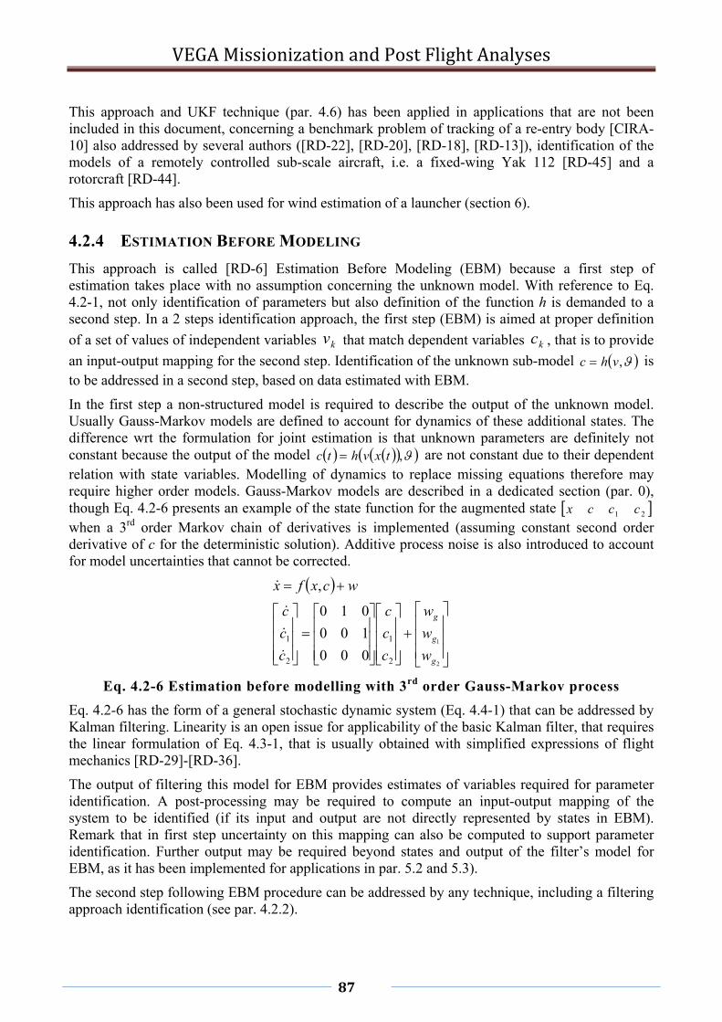
VEGA Missionization and Post Flight Analyses
87
This approach and UKF technique (par. 4.6) has been applied in applications that are not been included in this document, concerning a benchmark problem of tracking of a re-entry body [CIRA-10] also addressed by several authors ([RD-22], [RD-20], [RD-18], [RD-13]), identification of the models of a remotely controlled sub-scale aircraft, i.e. a fixed-wing Yak 112 [RD-45] and a rotorcraft [RD-44].
This approach has also been used for wind estimation of a launcher (section 6).
4.2.4 ESTIMATION BEFORE MODELING
This approach is called [RD-6] Estimation Before Modeling (EBM) because a first step of estimation takes place with no assumption concerning the unknown model. With reference to Eq. 4.2-1, not only identification of parameters but also definition of the function h is demanded to a second step. In a 2 steps identification approach, the first step (EBM) is aimed at proper definition
of a set of values of independent variables kv that match dependent variables kc , that is to provide
an input-output mapping for the second step. Identification of the unknown sub-model ,vhc is to be addressed in a second step, based on data estimated with EBM.
In the first step a non-structured model is required to describe the output of the unknown model. Usually Gauss-Markov models are defined to account for dynamics of these additional states. The difference wrt the formulation for joint estimation is that unknown parameters are definitely not constant because the output of the model ,txvhtc are not constant due to their dependent relation with state variables. Modelling of dynamics to replace missing equations therefore may require higher order models. Gauss-Markov models are described in a dedicated section (par. 0), though Eq. 4.2-6 presents an example of the state function for the augmented state 21 cccx when a 3rd order Markov chain of derivatives is implemented (assuming constant second order derivative of c for the deterministic solution). Additive process noise is also introduced to account for model uncertainties that cannot be corrected.
2
1
2
1
2
1
000
100
010
,
g
g
g
w
w
w
c
c
c
c
c
c
wcxfx
Eq. 4.2-6 Estimation before modelling with 3rd order Gauss-Markov process
Eq. 4.2-6 has the form of a general stochastic dynamic system (Eq. 4.4-1) that can be addressed by Kalman filtering. Linearity is an open issue for applicability of the basic Kalman filter, that requires the linear formulation of Eq. 4.3-1, that is usually obtained with simplified expressions of flight mechanics [RD-29]-[RD-36].
The output of filtering this model for EBM provides estimates of variables required for parameter identification. A post-processing may be required to compute an input-output mapping of the system to be identified (if its input and output are not directly represented by states in EBM). Remark that in first step uncertainty on this mapping can also be computed to support parameter identification. Further output may be required beyond states and output of the filter’s model for EBM, as it has been implemented for applications in par. 5.2 and 5.3).
The second step following EBM procedure can be addressed by any technique, including a filtering approach identification (see par. 4.2.2).

VEGA Missionization and Post Flight Analyses
88
4.2.5 GAUSS-MARKOV MODELS
Gauss-Markov models are used to model dynamic processes where no physical insight is applicable but causality can be addressed. A Markov model is basically defined by a chain of derivatives to represent some degree of continuity of a variable that is assumed to have Markov properties, as far as physical causal systems are addressed. An example of third order model is provided in Eq. 4.2-7. The general dynamics of the variable w are expressed in normal form introducing further states 21 ,, www , that are its first and second order time derivatives. The order of the model defines dynamic characteristics. Random process noise is also introduced as input in the Gauss-Markov model in order to represent uncertainties on this system. These are particularly useful in the frame of stochastic approaches as the case of Kalman filters.
2
1
0
2
1
2
1
000
100
010
w
w
w
w
w
w
Eq. 4.2-7 Gauss-Markov model of third order
The model of Eq. 4.2-7 has been adopted in [RD-1] and basically consists in approximating time profile with a parabola whose coefficients are to be corrected recursively by the filter in order to provide dynamic characteristics. It is a third order model with infinite correlation time, that is to say that current information impacts values in the far future (no forgetting factor is implemented). This model is suitable to have smoother corrections of the variable in a Kalman filter when relevant information from measurements is available. If poor feedback is available or in case of small sampling times, the model of Eq. 4.2-7 may result prone to instability and a proper time constant is to be addressed.
Eq. 4.2-8 presents the general form of a third order Markov process in normal form. Two equivalent representations are provided. The former has the advantage of having the poles of the system along the diagonal, being the state function represented by an upper triangular matrix. As time constants are evident, this form simply addresses correlation time characteristics. The latter has the advantage that further states are defined as time derivatives of the basic unknown, thus providing easier management in physical models (e.g. if wind gradient is to be introduced in parallel models). In this case dynamical characteristics are imposed in the last line, where the characteristic polynomial expression is reported. Simpler models with lower order are often defined to address unknown systems dynamics.
2
1
2
1
0
2
1
100
110
011
w
w
w
w
w
w
2
1
0122
1 100
010
w
w
w
pppw
w
w
Eq. 4.2-8 Representation of Markov models of third order
For instance a 2nd order model has been defined to address wind dynamics on VEGA launcher (par. 0) with a formulation (Eq. 6.5-5) whose deterministic contribution is a particular case of Eq. 4.2-8.
First order models have been used to address dynamics of corrections to aerodynamic or environmental models (see par. 5.2 and 5.3).
Typical expressions for parameter identification (Eq. 4.2-4) are also addressed by Eq. 4.2-8, if only the first line is considered.

VEGA Missionization and Post Flight Analyses
89
4.3 KALMAN FILTERING
The Kalman filter is an optimal state estimator for stochastic processes that was presented in 1960 [RD-7]. It was originally formulated for discrete time systems, but it is also applicable to continuous models. Due to efficiency, robustness, simplicity and performance it has been widely applied for state estimation of processes for whom noisy measurements are available.
Kalman filter has the typical architecture of state observers: error of estimation of measured output is fed back to the system in order to correct state estimates recursively.
Figure 4.3-1 State and output estimator
The feedback gain defines properties of the state observer, for instance it can be chosen in order to address error dynamics for asymptotic observers. In a Kalman filter, the so called Kalman gain is computed in order to address minimum mean square error of the estimate in presence of process and measurement noises. The theory is based on optimal Bayesian estimation [RD-7] and [RD-38].
In a Kalman filter we assume
a linear time-invariant system with additive zero-mean noises
Knowledge of state space matrix representation (A,B,C,D)
Availability of system inputs and measured outputs at each step
Defined covariance matrices for both process and measurement noises
The filter provides estimates of state and output and estimated covariance.
kkkk
kkkk
vHuDxCy
wGuBxAx
1
1
Eq. 4.3-1 Discrete linear stochastic model
Eq. 4.3-1 is a general representation of a linear dynamic system in discrete form. Last terms of state transition and output function are process and measurement white noise, characterized by respective covariance matrices Q and R. The former is meant to model uncertainty on the mathematical model, the latter represents measurement errors. The Kalman filter performs a compromise between two sources of information: mathematical model and available measurements. The compromise is an optimal solution for the stochastic problem according to given system (A, B, C, D) and noise (Q, R).
The implementation of Kalman filter can be divided in 2 phases:
I. Prediction (or time update)
II. Correction (or measurement update)
The former consists in prediction of propagation of the state estimate according to the system model. Predicted state estimate is indicated with a minus sign since only information from the past

VEGA Missionization and Post Flight Analyses
90
is used. Eq. 4.3-2 also shows prediction of state covariance assuming the system is linear and process noise is additive with zero-mean.
kkkk
kT
kk
kkkkk
DuxCy
QAPAP
uBxAx
1
11
Eq. 4.3-2 Prediction of state and its covariance
kk
kkkk
TT
PCKIP
yzKxx
RCPCPCK1
Eq. 4.3-3 Correction of state and its covariance
Eq. 4.3-3 is the correction phase, also called measurement update or a-posterior estimate, where information within current data is used to improve estimation throughout the innovation term
kk yzK . Eq. 4.3-3 also details recursive computation of the Kalman gain.
Remark that a Riccati equation provides a closed form solution for the Kalman gain that is optimal asymptotically, that is considering steady state solutions of the equation of state covariance matrix. This provides a-priori computed solution for the Kalman gain reducing recursive computation cost and providing a gain that only depends on a-priori information.
01 PBPBRQPAPA TT
Eq. 4.3-4 Algebraic Riccati Equation (ARE) for stationary solution
Kalman filters have encountered great success, in particular to deal with sampled noisy measurements. The stochastic formulation provides estimates of the first and second statistical moments, namely expected values and variance of state variables. In engineering application the expected value is assumed as the best estimation and its variance is used to represent confidence on such estimation.
As most aerospace applications deal with non-linear time-varying systems, assumptions within the original Kalman filter had to be overcome. For what concerns non-stationarity of the system, the same approximations usually accepted for control systems design is carried on:
o system variation with time is supposed slower than states dynamics,
o frozen systems are addressed in a time slice approach,
o gain scheduling or switching is introduced to deal with time-varying properties.
The subject of non-linearity is more complex and only recent evolutions of Kalman filtering consider the non-linear problem.
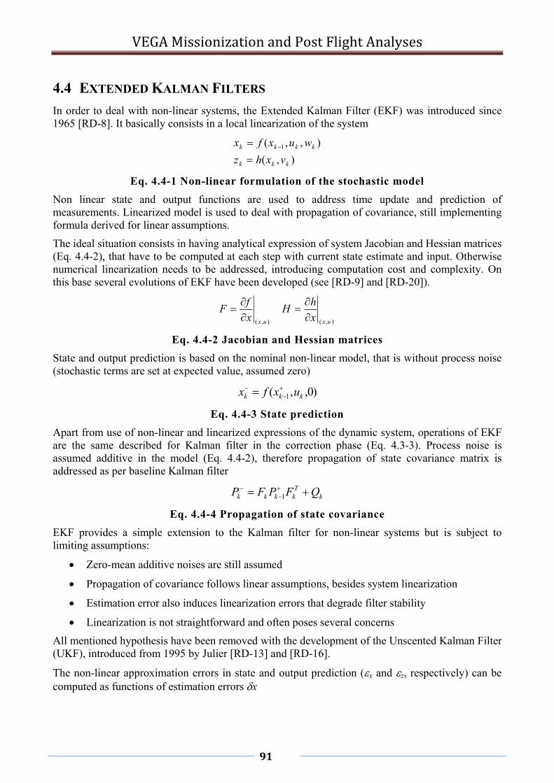
VEGA Missionization and Post Flight Analyses
91
4.4 EXTENDED KALMAN FILTERS
In order to deal with non-linear systems, the Extended Kalman Filter (EKF) was introduced since 1965 [RD-8]. It basically consists in a local linearization of the system
),(
),,( 1
kkk
kkkk
vxhz
wuxfx
Eq. 4.4-1 Non-linear formulation of the stochastic model
Non linear state and output functions are used to address time update and prediction of measurements. Linearized model is used to deal with propagation of covariance, still implementing formula derived for linear assumptions.
The ideal situation consists in having analytical expression of system Jacobian and Hessian matrices (Eq. 4.4-2), that have to be computed at each step with current state estimate and input. Otherwise numerical linearization needs to be addressed, introducing computation cost and complexity. On this base several evolutions of EKF have been developed (see [RD-9] and [RD-20]).
),(),( uxux x
hH
x
fF
Eq. 4.4-2 Jacobian and Hessian matrices
State and output prediction is based on the nominal non-linear model, that is without process noise (stochastic terms are set at expected value, assumed zero)
)0,,( 1 kkk uxfx
Eq. 4.4-3 State prediction
Apart from use of non-linear and linearized expressions of the dynamic system, operations of EKF are the same described for Kalman filter in the correction phase (Eq. 4.3-3). Process noise is assumed additive in the model (Eq. 4.4-2), therefore propagation of state covariance matrix is addressed as per baseline Kalman filter
kT
kkkk QFPFP
1
Eq. 4.4-4 Propagation of state covariance
EKF provides a simple extension to the Kalman filter for non-linear systems but is subject to limiting assumptions:
Zero-mean additive noises are still assumed
Propagation of covariance follows linear assumptions, besides system linearization
Estimation error also induces linearization errors that degrade filter stability
Linearization is not straightforward and often poses several concerns
All mentioned hypothesis have been removed with the development of the Unscented Kalman Filter (UKF), introduced from 1995 by Julier [RD-13] and [RD-16].
The non-linear approximation errors in state and output prediction (x and z, respectively) can be computed as functions of estimation errors x

VEGA Missionization and Post Flight Analyses
92
xx
hxhxxhKx
x
fxfxxf zx
Eq. 4.4-5 Estimation errors induced by non-linearities in the model
Errors in Eq. 4.4-5 are deterministic sources of error on state update and output computation, respectively, induced by the linear approximation of the system. They need to be covered by means of the variance of process and measurement noise, respectively, though they are not gaussian.
Besides effects of linearization, it is to be remarked that propagation of stochastic characteristics is not correct, because linear assumptions are not applicable
)0,,()0,,( 11 kkkkkk uxEfuxfExEx
Eq. 4.4-6 Propagation of expected value
This is better address by the recent approach of the Unscented Transformation.

VEGA Missionization and Post Flight Analyses
93
4.5 UNSCENTED TRANSFORMATION (UT)
Unscented Kalman Filter is based on the so called Unscented Transformation introduced by Julier and Uhlmann in 1995 [RD-16]. This transformation is meant to address the problem of reproducing statistical moments (mean and covariance) of a vector on the base of a subset of perturbations. Motivation was developed in the frame of Kalman filtering for non-linear systems and the original idea that it is easier to approximate statistical moments rather than linearizing a system.
Given a stochastic vector defined by expected value 0x and covariance matrix P, considering a
non-linear function
)( 0xhy
Eq. 4.5-1 Non-linear propagation function
the Unscented Transformation (UT) aims at estimation of expected value and covariance of the output, since linear assumptions are not applicable
PHHyEyE
xEhyET
2
0 )(
Eq. 4.5-2 Propagation of mean and covariance for linear transformations
The UT follows the steps
I. Generation of the so-called sigma points i
II. Definition of corresponding weights iW
III. Application of the function to all sigma points
IV. Computation of weighted mean and covariance of output sigma points
It is not a numerical statistical process like Monte Carlo simulations or Particle filters ([RD-25], [RD-23]) because sigma points are a limited deterministic set, i.e. not statistically relevant but deterministically selected. The name of sigma points is probably due to the original formulation
where these points were generated as perturbations of each component of 0x with plus and minus
its standard deviation . Several formulations for sigma points generation are possible ([RD-13], [RD-14], [RD-15], [RD-17] and [RD-19]) but we focus on the one that has been considered more efficient. Further details can be found in mentioned literature and have been discussed in [D2.1PI].
Sigma points are defined as perturbations around the mean value 0x of the given stochastic vector
and 0x itself, also called central point.
ii Px 0
Eq. 4.5-3 Sigma points for Unscented Transformation
This provides a base of 12 N vectors where N is the size of 0x . The second addendum on right
side is the ith column of the matrix square root of the covariance matrix P, scaled by the design parameter . The latter is used to address higher order moments of the distribution and is usually set to 3 to address gaussian distributions [D2.1PI].

VEGA Missionization and Post Flight Analyses
94
Definition of weights is another subject that has been extensively discussed in [D2.1PI]. If all
weights are chosen equal apart from the weight for central point 0 , the condition N
WWi 2
1 0
holds to provide complement to 1, therefore
N
W
NiWi
1
2..1;2
1
0
Eq. 4.5-4 Weights for sigma points in UT
These weights can also be negative and are only meant to provide linear combination of sigma
points resulting in a mean 0x and a mean squared error P.
Once sigma points and weights are defined, Eq. 4.5-1 is computed for each sigma point of Eq. 4.5-3
providing propagated sigma points )( ii h .
UT assumes that the set of transformed points is an approximation of the first statistical moments of
a stochastic process defined by ( 0x , P) across the non-linear function of Eq. 4.5-1. Remark that
first and second order statistical moments are sufficient for Kalman filter derivation. These are computed as weighted average and mean squared error of output sigma points
i iiWy 0
i
Tiiiy yyWP 00
Eq. 4.5-5 Approximation of expected value and covariance matrix
The covariance matrix is composed by expected values of cross-correlation between components
jjhhjh yEyyEyEP
A typical example of the effectiveness of UT for non-linear systems is presented in several papers reproducing a figure from [RD-13]. A basic example is here reproduced to show the effect of non-linearities in the frame of stochastic estimation.
The chosen non-linear function consists in transformation from cartesian to polar co-ordinates, whose expression is not reported. A stochastic position is defined in the cartesian plane with coordinates having expected value of (0, 5) and standard deviations (3, 0.5). Figure 4.5-1 presents a statistical set of 10000 realizations (yellow dots), mean point of the distribution and the corresponding uncertainty ellipsoid. Sigma points are defined for UT are also shown. Remark that the formulation presented in this work (red crosses) is compared with the so-called scaled UT [RD-15] introduced to avoid excessive spread of sigma points (green). Remark that an asymmetrical dispersion has been purposely defined, addressing mainly azimuth in polar coordinates wrt origin (0, 0).
Expected value and covariance matrix (represented through the uncertainty ellipsoid) are computed in the polar coordinates with different methods:
Monte Carlo approach with a statistical representation (exact solution)
EKF approach, that is non-linear transformation for mean value and Jacobian to address propagation of covariance (as discussed for EKF)
Unscented Transformation described in this section
Scaled UT

VEGA Missionization and Post Flight Analyses
95
Figure 4.5-2 reports results in the polar coordinates plane.
Due to non-linearities and relevant dispersion, the output distribution is not fairly represented by an ellipsoid, requiring higher order statistical moments. Remark that, due to the banana shape of the distribution, the expected does not match transformation of the nominal position. This offset is not addressed by EKF approach but is accurately estimated by UTs. Remark that the simpler UT provides a more accurate estimation of covariance, due to the wider spread of sigma points, particularly relevant in the transformed coordinates.
This example highlights the positive outcome of UT in propagation of mean and covariance throughout non-linear systems. The polar to cartesian transformation is often encountered in engineering applications, in particular for tracking problems [RD-22], since both sonar and radar are affected by accurate range measurements but dispersed angles.

VEGA Missionization and Post Flight Analyses
96
Figure 4.5-1 Stochastic realisation in cartesian coordinates
Figure 4.5-2 Statistical properties in polar coordinates
-10 -5 0 5 10
-4
-2
0
2
4
6
8
10
12
14
x1
x 2
Piano Cartesiano
dati
mediavarianza
punti sigma
0 20 40 60 80 100 120 140 160 1802
4
6
8
10
12
14
16
[°]
R
Piano Polare
datimedia
varianza
stima lineare
stima var lineare
punti sigma UTstima UT
stima var UT
punti sigma UTscaled
stima UTscaledstima var UTscaled

VEGA Missionization and Post Flight Analyses
97
4.6 UNSCENTED KALMAN FILTER (UKF)
The Unscented Kalman Filter (UKF) is a formulation of the optimal Bayes recursive estimator where propagation of expected value and covariance of the state estimate is addressed by means of the UT. The UKF is based on the idea [RD-13] that it is easier to estimate statistical properties rather than linearizing a system and apply linear theory as per EKF.
),(
),,( 1
kkk
kkkk
vxhy
wuxfx
Eq. 4.6-1 Non-linear stochastic model
In particular the UT is used to deal with both state transition function and output function. No assumption is required of linearity, nor possible linearization of the system. Process and measurement noises are not necessarily additive nor need to have zero-mean. The UT is capable of taking into due account all these events.
UKF implementation requires 3 main steps:
I. Definition of the augmented state and UT
II. Prediction phase by means of UT
III. Correction phase with general formulas of Kalman filters (Eq. 4.3-3)
Given a non-linear stochastic process (Eq. 4.6-1), derivation and implementation of UKF is discussed in what follows. More details are reported in [D2.1PI].
This technique has been extensively applied in several system identification problems:
A benchmark for tracking of a re-entry body [CIRA-9]-[CIRA-10], often used in literature ([RD-22], [RD-18], [RD-16]) aiming at primary use and comparison with other techniques [CIRA-11]
Methodological developments for CIRA USV ([D1.3PI], [D2.1PI] and [D2.2PI])
applications to realistic simulations and flight data ([RD-1], [RD-2] and [RD-3])
typical problems in aircraft ([RD-39], [RD-44], [RD-45])
4.6.1 IMPLEMENTATION OF UT WITHIN THE FILTER
For the sake of clarity, only the complete formulation of UKF is here described, also called augmented UKF [RD-20]. The UT is applied to an augmented state vector defined appending process and measurement noises to the filter’s state.
Given a system (Eq. 4.6-1) characterized by
state x of dimension N ,
qN process noises ( w) with covariance Q and
rN measurement noises ( v ) of covariance R,
UT is applied to an augmented state of dimension rqa NNNN , defined as

VEGA Missionization and Post Flight Analyses
98
v
w
x
xa
Eq. 4.6-2 Augmented state for UT within UKF
Application of UT requires definition of both expected value and covariance of the augmented state Eq. 4.6-2. Expected value of filter’s state corresponds to previous step estimate, as already performed by Kalman filters. Expected value of process noise is usually zero, though this algorithm is capable to deal with time-varying bias errors, if known in advance.
k
k
k
a
vE
wE
x
xEx1
0
Eq. 4.6-3 Expected value of augmented state
Augmented covariance is composed by filter state, process noise and measurements noise covariance on diagonal blocks and zeros to complete the matrix, where no correlation is assumed.
R
Q
P
P
qrr
rqq
rq
NNNN
NNNN
NNNNk 1
Eq. 4.6-4 Covariance of augmented state
This operations are carried out at each step during recursive filtering, therefore time-varying profiles for covariance of process and measurement noises can be considered, if necessary.
State and output function need to be augmented correspondingly, though it is merely a formal issue
to allow for implementation of the UT. The outcome is the generation of 12 aNN sigma
points, according to above mentioned assumptions for UT and for augmented state.
aikNi
k
aiki
NiPx
x
NiPx
a..1;
;
..1;
1
10
1
Eq. 4.6-5 Sigma points generation on augmented stochastic vector
aa
i
a
NiN
WW
NW
2..1;2
1
2
1
1
0
0
Eq. 4.6-6 Weights for sigma points of augmented state
Different set-up can be implemented in simpler cases. For instance, when additive zero-mean noises are considered, it is useless to have an augmented UT to deal with their effect, since Eq. 4.5-2 can be applied. Remark that an intermediate generation of sigma points is required if state is not augmented with process noise [RD-18]. These solutions have been widely experienced in the framework of development of Post Flight Analysis for CIRA USV ([D1.3PI], [D2.1PI] and [D2.2PI]) but also within final applications ([RD-1], [RD-2] and [RD-3]).

VEGA Missionization and Post Flight Analyses
99
4.6.2 PREDICTION BY MEANS OF UT
The prediction phase of the UKF is carried out as follows
kia
ki
ki
kikki
ki
ki
ki
i uf
v
w
wuxf
v
w
x
X ,
),,( 1
Eq. 4.6-7 Time propagation of sigma points by means of augmented state function
i iik XWx
Eq. 4.6-8 A-priori estimate of state as weighted average
i
T
kikiik xXxXWP
Eq. 4.6-9 A-priori estimation of state covariance as mean squared error
iakikii XhvxhY ),(
Eq. 4.6-10 Estimation of output for each realization of propagated sigma points
i iik YWy
Eq. 4.6-11 Estimation of output as weighted average
i
Tkikiiyy yYyYWP
Eq. 4.6-12 Estimation output covariance
i
Tkikiixy yYxXWP
Eq. 4.6-13 Estimation of cross correlation of output and state
Sigma points are fed to augmented state transition function providing the transformed set. State prediction and covariance estimation are computed as weighted mean and squared error. Estimation of output is also computed on the base of the transformed set. Expected value of output is computed along with output covariance estimation and cross-correlation of state and output. Remark that measurement noise has been accounted for, since Kalman filter is basically addressing estimation of measurements (possibly including sensor noise).
4.6.3 CORRECTION OF KALMAN ESTIMATE
The specific operations of UKF are in the prediction phase, where the computation is addressed by UT. The correction phase is basically the same of any Kalman filter
kkk yz
yyxy PinvPK
kkk Kxx
Tyykk KPKPP
Eq. 4.6-14 Correction phase of Kalman filtering

VEGA Missionization and Post Flight Analyses
100
Kalman filtering (or better optimal Bayes recursive estimation), is based on
computation of the Kalman gain, feedback of state observer,
innovation term, addressing information from real measurements,
correction of state estimate, posterior estimate or measurement update and
correction of state covariance estimation.
4.7 SUMMARY ON DEFINITION OF A KALMAN FILTERING PROBLEM
In this section a brief summary of most relevant items necessary to address systems identification with a filtering approach method is provided.
The main elements in Kalman filtering are
a) Definition of the filter’s model to address the stochastic problem
b) Definition of algorithm implementation
c) Covariance of process and measurement noises
d) Initial conditions for state and covariance
Last point (d) is used to address a-priori information. Initial condition of filter’s state is important for filter’s convergence in case of non-linear applications (EKF) because it defines the set point. When possible, a sort of inversion of measurements at first available instant is used to define initial conditions. Initial conditions are also critical for parameter identification because they define a-priori the model and allow accounting for a first guess of the system to be identified. Initial conditions of state covariance matrix are used to address filter’s performance in the initial phase, in particular to address higher convergence rate at the beginning, for instance when measurements bias is to be caught. It is usually a diagonal matrix for states whose correlation is not a-priori known. The main diagonal is made of variance of each state variable, that represents uncertainty on the initial condition.
Covariance of process and measurement noise (c) are items that complete definition of the stochastic model but are often heuristically used as tuning parameters during filter design, in particular process noise covariance. A diagonal form is often implemented to represent uncorrelated noises. Measurement noise is more likely defined in order to characterize sensors accuracy, therefore representing actual characteristics of the model.
Definition of algorithm implementation (b) implies several aspects of detail. The basic choice of algorithm among baseline Kalman filter, EKF, UKF, etc. has to be addressed first. For EKF, further possibilities for linearization include: analytical formulations (Jacobian and Hessian matrices); numerical recursive linearization; use of scheduled linearized systems in case of a-priori known reference conditions, as it is likely with launchers. Further improvements of convergence are possible [D2.1PI].
In case of UKF, choices regard augmentation of the state with process and measurement noise for implementation of UT. A single UT to deal with both state and output function may be replaced by two separate UTs, the so-called regeneration [RD-18]. Definition of the UT also includes several options in terms of analytical definition ([D2.1PI], [RD-19], [RD-17], [RD-15]) or numerical implementation ([RD-14], [RD-20], [RD-9]).
Further implementation issues deal with integration of continuous models (a-b), where different methods can be applied. First order Euler method guarantees linearity of the system but is suitable for sampling periods up to 0.02 s (50 Hz) in aerospace applications [RD-22]. Runge-Kutta 4th order

VEGA Missionization and Post Flight Analyses
101
method is implemented otherwise. If measurement sampling is too low, numerical integration can be performed with intermediate steps.
Definition of filter’s model (a) is the primary issue. In particular the stochastic problem is defined which is basic and more important than its solution. Output and sampling period is usually based on available measurements. Virtual measurements can be introduced to support use of further information [RD-2]. In this phase it is important to decide what is to be estimated (unknown filter’s states) and what is not: neglected degrees of freedom, uncertain parameters addressed by process noise, inputs, etc. For un-modeled dynamics and uncertainties, recovery actions need to be defined, for instance further process noise. Assumptions and modeling are also affected by implementation issues such as linearity, stationarity, etc. that are to be addressed by filter’s implementation (b).

VEGA Missionization and Post Flight Analyses
102
5 UNSCENTED FILTERING FOR PRORA-USV
The non-linear stochastic technique of the Unscented Kalman Filter has been applied within PRORA-USV to improve knowledge of aerodynamic characteristics of the prototype re-entry vehicle FTB. The program (PRORA-USV), the vehicle (FTB) and scheduled missions (DTFT) have been introduced at par. 0.
Estimation before modelling approach has been chosen to address in a second step the problem of parameter identification for the complex aerodynamic model in transonic regime.
In what follows, details on application to PRORA-USV are provided concerning simulated and flight data of 2 missions, called DTFT (Dropped Transonic Flight Test). These applications have been presented in papers
Simulated data of DTFT 1 [RD-1]
Flight data from DTFT 1 [RD-2]
Simulated data of DTFT 2 [RD-3]
Further activities have been carried out before and after these applications in order to test the technique. In particular the joint estimation approach has been applied ifor
o A benchmark problem of tracking of a re-entry body [CIRA-9]; it has been addressed with UKF [CIRA-10] and results compared [CIRA-11] with another technique developed at CIRA, called FTR (Fourier Transform Regression). This showed the high potential of the UKF non-linear technique.
o Further fields of application are related to scale models of both fixed wing and rotor-craft, carried out with students at DMA (Dipartimento di Meccanica e Aeronautica). Applications have been limited to simulated data because of major problems during flight testing of the small remotely controlled vehicles of DMA. UKF has been used to correct aerodynamic derivatives of the model representing a small scale Yak -112 [RD-45] and an helicopter with stabilizing fly-bars [RD-44].
This work mainly focused on developing a methodology for systems identification and is described in par. 5.1. Next sections describe following applications carried out at CIRA on flight data (par. 5.2) and on simulated data of a second mission (par. 5.3).
5.1 DEVELOPMENTS WITH SIMULATED DATA OF DTFT 1
This section summarizes the identification of the aerodynamic model of the Unmanned Space Vehicle (USV) designed and produced at the Italian Aerospace Research Center (CIRA) as an experimental platform for the development and demonstration of enabling technologies for future generation aerospace vehicles.
System identification aims at upgrading the aerodynamic database of the USV, developed through wind tunnel testing of sub-scale models and CFD, for the purpose of flight control system design in the extended flight envelope of the vehicle.
Estimation of the parameters of a suitably structured aerodynamic model of the unpowered and reusable vehicle is carried out as a nonlinear filtering problem, in the framework of a multistep approach where the aerodynamic coefficients are identified first and, in a following phase, the unknown parameters are adjusted. The Unscented Kalman Filter is used as a recursive parameter estimation algorithm.

VEGA Missionization and Post Flight Analyses
103
The methodology has been applied to data generated by a realistic simulation model of the vehicle and its sensor suite, to assess the filtering performance of the algorithms in state and parameter estimation. Results were presented at AIAA Atmospheric Flight Mechanics Conference 2007 [RD-1].
5.1.1 SYSTEMS IDENTIFICATION STRUCTURE
Systems identification of FTB 1 vehicle from DTFT data is very challenging because the flight test manoeuvres, usually performed for the purpose of aerodynamic model extraction, are not scheduled during the DTFT. Moreover, DTFT is a one shot mission, characterized by a wide flight envelope, providing a limited number of suitable data together with no reproducibility (in the short term) of the experiment. Finally, aerodynamics is very sensitive in transonic regimes where linear models are poorly suited to describe aerodynamic forces and moments acting on the vehicle.
An aerodynamic database (ADB) of the FTB 1 has been developed at CIRA in the whole range of envisioned flight conditions from subsonic up to low supersonic regime with particular focus on the transonic region.
As the first USV FTB 1 mission, performed in February 2007, should be followed by further flights (next is sheduled by the end of 2009), validation and update of original ADB from flight data is being used to support the development of an updated version of the flight control software capable of reliably and accurately manage the vehicle trajectory in the extended flight envelope (up to Mach 2) foreseen for the future scheduled missions of the USV. To this end, an analytical model has been extracted by the ADB, the structure of which is based on first principles and specifically accounts for the nonlinearity of the aerodynamic model of the winged body FTB 1 vehicle and, more important, for the significant variation of flow characteristics from low subsonic through supersonic regime.
The identification process aims at determining incremental updates of the parameters of the analytical model, where necessary, so as to correct and adjust the original database. The combined problem of state and parameter identification is formulated as a nonlinear filtering problem and solved according to the Estimation Before Modelling approach where aerodynamic coefficients are estimated first and, in a second phase, the parameters of the aerodynamic model are adjusted.
The identification problem deals with the expression of the aerodynamic force and moment coefficients that can be expressed as follows in concise form
,,uxhc
Eq. 5.1-1 General expression of aerodynamic model
where h is a general nonlinear real-valued function (once the aerodynamic model is suitably structured) with inputs composed of independent variables related to the vehicle state x and controls u, and a vector of constant parameters . Accordingly, the vehicle dynamics can be described as
cuxgy
cuxfx
,,
,,
Eq. 5.1-2 General expression for vehicle dynamics
Estimation Before Modelling (EBM) is a 2 step approach where estimation of state x and generalized forces c is first performed while parameter identification is carried out in the second step. This procedure has been described in par. 4.2.4. Furthermore, the first step of the EBM has been split into two sub-problems, to address separately problems related to wind and air-sensor data and inertial filtering. The three steps procedure is outlined in what follows:

VEGA Missionization and Post Flight Analyses
104
Inertial estimation and filtering. The first problem deals with filtering measurements from the Inertial Measurements System (IMS) and estimation of the state of the FTB 1 along with forces and moments. We make use of the standard equation of motion for the vehicle and of Markov chains for the un-modelled aerodynamic loads.
Air properties estimation and filtering. The second problem consists of filtering measurements from Air Data System (ADS) and estimation of wind components along with air state variables. We use FTB 1 state as an input (from first problem), and dynamics for unknown variables are modelled as Markov chains of appropriate order.
Parameter identification. After solving problems 1. and 2. we can calculate non-dimensional aerodynamic coefficients in air reference coordinates (c) to be used for parameter identification. Independent variables of the aerodynamic model are also ready for use after filtering from measures.
In all phases the Unscented Kalman Filter (UKF) technique is used, where the probability distribution of the stochastic variables is approximated using a deterministic set of sample points.
The adopted approach has been evaluated via simulation using a 6 DOF model of the vehicle where the ADB is implemented and FCS and sensor dynamics are described in detail. The simulation of first FTB 1 mission is used to generate appropriate input data for the estimation procedure to address the issues of observability and identifiability of model parameters, and to define the characteristics of the filters and assess the overall performance of the identification procedure. In this respect, note that the mission profile could not be modified during the maiden flight of FTB 1 where the command inputs are generated by the FCS to accurately track the programmed trajectory, and no specific manoeuvre could be executed for the purpose of aerodynamic model extraction.
5.1.2 FIRST STEP: ESTIMATION BEFORE MODELLING
In the first step measurements from INS are used to address rigid body motion in 6 dof. As vehicle state is completely measured, Kalman filtering is aimed at estimation of forces and moments acting on the vehicle, for whom no physical model is used in this phase.
Measurements are available with 100 Hz sampling rate and addressing 15 variables:
hLonLatWVUrqpaaaz zyxk ,,,,,,,,,,,,,,
Position in ECEF (Earth Centered Earth Fixed) coordinates, velocity components in NED (North East Down) frame, acceleration components in body frame. For attitude dynamics, body frame components of angular rate and Euler angles describing rotation from ECEF to body frame.
Vehicle state for 6 dof motion is defined with Euler angles, NED positions, body frame components of translational and rotational velocity:
rqpwvuZYXx EEEv ,,,,,,,,,,,
Eq. 5.1-3 is a general expression of equations of motion (with standard nomenclature of mentioned variables) under the assumption of constant mass properties. Gravity is assumed known exactly while no physical information is used to define a model for aerodynamic loading.
a
ag
MII
FFvvm
Eq. 5.1-3 Equations of motion

VEGA Missionization and Post Flight Analyses
105
A Gauss-Markov model is introduced to address dynamics of aerodynamic loads aa MFa , . In
particular a third order model with infinite correlation time (see par. 0) has been chosen in congruence with [RD-6] and [RD-11]. This model is described by Eq. 5.1-4, where loads
aa MFa , and their derivatives are driven by process noise 210 ,, www .
22
121
01
wa
waa
waa
Eq. 5.1-4 Gauss-Markov model for aerodynamic loads and derivatives
A general state transition function kk xfx 1 for the filter is derived in the following steps:
An augmented state is defined as 21,,, aaaxx v
Eq. 5.1-3 is expanded and recast in normal form wrt selected state (details are omitted because general equations of flight mechanics are concerned)
Eq. 5.1-4 is appended to complete filter’s state function
A numerical integration method is implemented (i.e. Euler first order explicit method with 0.01 s step)
This provides a non-linear expression of equations of motion, that is completed by the output
function 11 kk xgy . Detailed Simulink model for sensor simulation have been directly
implemented in the filter, standing the capability of UKF to use any sort of filters model as a black box.
The outcome is a complex model with
o 15 output
o No input
o 30 states, that is
12 vehicle states for 6 dof rigid body dynamics,
18 to address 3rd order models of 6 components of loading
As both process and measurement noise are additive zero-mean in state and output equations, a simplified implementation of UKF has been preferred: the Unscented Transformation has been
applied with no state augmentation, resulting in a set of 6112 xNN points.
Further details on modeling and implementation are provided in [D2.2PI] and more extensively discussed in [D2.1PI].
An example of results achieved is presented in Figure 5.1-1 and Figure 5.1-2. The former compares estimated pitch angle (blue line) with the available measurements (red dots), showing that the trajectory has been properly tracked by the filter, despite no information on forcing actions. Estimation error is lower than uncertainty bounds of sensor noise, therefore the filter provides adequate tracking of measurements and smoothing of related noise.
The great performance of UKF is demonstrated in Figure 5.1-2, where normal aerodynamic force is shown, that is close to lift force standing little angles of attack. Aerodynamic forces are accurately estimated along with their dynamics.

VEGA Missionization and Post Flight Analyses
106
Figure 5.1-1 Comparison of estimation and estimation error for pitch attitude
Figure 5.1-2 Comparison of estimation and error on lift force

VEGA Missionization and Post Flight Analyses
107
5.1.3 SECOND STEP: AIR ESTIMATION
In the second step air properties are estimated on the base of
available measurements from ADS (Air Data System)
information concerning vehicle motion from first step
aerodynamic characteristics.
The unknowns are sswwwADS TPWVUx ,,,, , where wind components in inertial reference frame
define air motion and static pressure and temperature define air state. A Gauss-Markov model of 3rd order has been defined for wind components with infinite time constants (see par. 4.2.4) as it provides a general representation of unknown dynamics [RD-43]. A second order model has been chosen for air state since smoother profiles are expected.
Furthermore the small sample period at which measurements are available ( s01.0 ) is small wrt expected dynamics therefore implementation of a simple first order Euler method with the same step is representative enough to propagate the continuous model across intervals of measurements. Therefore state transition for the filter state is
kW
W
W
S
S
W
W
W
S
S
W
W
W
kW
W
W
S
S
W
W
W
S
S
W
W
W
W
V
U
T
P
W
V
U
T
P
W
V
U
W
V
U
T
P
W
V
U
T
P
W
V
U
1000000000000
0100000000000
0010000000000
0001000000000
0000100000000
000010000000
000001000000
000000100000
000000010000
000000001000
000000000100
000000000010
000000000001
1
Eq. 5.1-5 State transition function for second step filter
Resulting in a linear discrete model. Additive zero-mean process noise are considered for highest order derivatives of the unknowns and variance are defined as tuning parameter.
Above mentioned assumptions allow for implementation of the simplest form of the Kalman filter for state update
kk xAx 1
kTx
kx
k QAPAP 1
Eq. 5.1-6 Propagation of state and covariance for linear model
The dedicated model regards implementation of the output function that is more complex, non-linear and time-varying, therefore UKF is more suitable. This is in contrast with common
VEGA Missionization and Post Flight Analyses
108
applications of Kalman filtering, where non linear state function are addressed while output functions are basically a subset or linear combinations of state variables.
The output function is in charge of computing estimated values of current measurements, that are static and total pressure from Pitot probe, total temperature, aerodynamic angles from wind vanes.
,,,, TTSADS TPPy
A Simulink model, also suitable for simulation, is used to implement the processing required to compute output based on following vectors of input
air state sswwwADS TPWVUx ,,,, , i.e. first 5 components of the second step filter’s state
vehicle state, whose time profile is provided by first step estimation
First of all air relative velocity is computed with components in body reference frame. For this purpose Euler angles are used to have both vehicle and wind velocity in body frame. Euler angles, estimated at first step, are here used as input along with its estimated covariance matrix.
NED
NED
NED
b
b
b
W
V
U
R
w
v
u
,, and
w
w
w
b
b
b
a
a
a
w
v
u
w
v
u
w
v
u
True Air Speed (TAS) and aerodynamic angles are then computed with
TAS
varcsen
u
warctg
wvuTAS
a
a
a
aaa
222
Aerodynamic angles are measured output while the air speed is required for computation of total pressure and temperature. Air density is computed with state equation for air based on static temperature and pressure that are estimated recursively
T
P
05.287
2
2
1TASPdin
This allows for a recursive estimation of dynamic pressure, that is a further output required for 3rd step of estimation, since aerodynamic loads are a-dimensionalized accordingly.
Total temperature and pressure are function of Mach number according to the equations of compressible gas-dynamics, that are, for air
2
5.32
2.01
2.01
MTT
MPP
ST
ST
Static pressure and temperature are filter states while Mach number is computed with TAS and sound speed, that is
sRTTASM

VEGA Missionization and Post Flight Analyses
109
Further modelling of air sensors and tubing effects of Pitot probe are accounted in the model implemented, but details are discussed in [D2.2PI] and [CIRA-6]. What is worth to be mentioned here is that sensor error is not addressed by additive random noise only, but a non-stationary component is also present, related to angle of attack (performance of static and dynamic pressure intakes) and dynamic pressure (accuracy of calibration curves).
The outcome is a filter’s model with
o a simple linear state function (Eq. 5.1-5) with additive process noise
o 13 states, that is 5 unknowns for atmosphere ( sswwwADS TPWVUx ,,,, ) and their
derivatives according to Markov chains
o A complex non-linear output function, derived from sensors models
o 5 output, corresponding to measurements of ADS ( ,,,, TTSADS TPPy )
o 6 input from vehicle state estimation at first step (attitude and velocity)
Input to the output function kvkk vkxxgy ,1,11 are, in the order,
Atmosphere state ADSx , namely the state of 2nd step filter (only 5 components are actually
required)
Vehicle FTB_1 state ( Vx ), that is used as an input in second step estimation (only Euler
angles and velocity components are necessary)
Bias errors on pressure sensors, assumed known from previous calibration and estimation during ascent phase
Non additive errors () on pressure sensors, to be computed recursively as function of current dynamic pressure and angle of attack
Additive sensor noise is not fed directly to the model.
Linear Kalman filtering equations are used to address state transition, standing the linear state function with additive zero-mean process noise. A non-augmented UT has been implemented, with 27 sigma points, to address non-linearity of output function.
The variance of sensor noise is computed recursively to account for sensors scale factors:
,1 DINkaddkUTyyyy PRRxPP
Remark that the simplified implementation was justified by accuracy of results of first step estimation. More complex forms of UKF implementation have been discussed in [D1.3PI]. In particular, definition of an input augmented UT has been discussed. In this case covariance matrix of input is properly accounted besides current state covariance. For instance vehicle state is an input in 2nd step filtering and it is provided after 1st step estimation (EBM) along with estimated covariance matrix.
Results of 2nd step estimation are summarized in Figure 5.1-3 and Figure 5.1-4. More extensive results are presented in [D2.2PI]. Estimated values of angle of attack are compared with corresponding measurements, proving that this variable is properly estimated (despite no deterministic model is used) and its time profile is smoother wrt noisy measurements (filtering). For what concerns wind estimation, estimated profile is congruent with simulated profile, except at the end of the mission where high vehicle speed makes wind effects negligible, i.e. not detectable.

VEGA Missionization and Post Flight Analyses
110
Figure 5.1-3 Filtering of angle of attack
Figure 5.1-4 Wind estimation

VEGA Missionization and Post Flight Analyses
111
5.1.4 THIRD STEP: PARAMETER IDENTIFICATION
The third step consists in parameter identification to address aerodynamic model of FTB_1. The objective is correction of parameters of an analytical model dedicated to representation of aerodynamics across all regimes of flight: sub-sonic, transonic and supersonic.
This analytical model has been developed for [D1.2PI] and presented in [RD-4].
Input are RAErqpM ,,,ˆ,ˆ,ˆ,,, , namely
Mach number
Aerodynamic angles
Reduced angular rates for rotary effects
Deflection of aerodynamic surfaces (controls)
The model is based on physical insights to provide
o sufficient flexibility to support model correction for system identification
o limited degrees of freedom to avoid unacceptable forms
These aspects are mostly related to Mach dependence. A separation principle is introduced, therefore analytical expressions of aerodynamic coefficients are defined with Mach dependent parameters in the following form
),,,ˆ,ˆ,ˆ,,(),(
,,,ˆ,ˆ,ˆ,,,],,,,,[
,
17
1
, RAEji
j
jii
RAEnmlLYD
rqpGxMFc
rqpMvCCCCCCc
Eq. 5.1-7 Separation assumption for aerodynamic coefficients
For instance, drag and lift coefficients are
2171615
2141312
211109
8765
24
2232
21
ˆˆˆcoscoscos
coscoscos
RRR
AAA
EEE
D
FFF
FFF
FFF
senpFrFqsenFF
senFsenFsenFFC
2171615
2141312
311109
8765
24
2232
21
ˆˆˆcoscoscos
coscoscos
RRR
AAA
EEE
L
FFF
FFF
FFF
senpFrFqsenFF
senFsenFsenFFC
Eq. 5.1-8 Analytical expressions for aerodynamic coefficients
Eq. 5.1-8 provide a general form that is more suitable than common linear models, that can be derived as the Hessian of Eq. 5.1-8. Control surfaces are addressed by additive terms wrt baseline aerodynamics with zero deflection. Mach dependence is implicit in the coefficients, Fj, for whom a further analytical expression is given

VEGA Missionization and Post Flight Analyses
112
2
1
2
1supsup2
32
21
01
1
1
1y
y
subjMg
MgHF
Mm
MhMhmHFMF
2
1150tanh,
2
1150tanhsup
MMH
MMH sub
Eq. 5.1-9 Expression of Mach form factors
Eq. 5.1-9 is used to address most relevant typical characteristics of aerodynamic coefficients as function of Mach number, as known from theory and literature. For instance Eq. 5.1-9 imposes
o in low sub-sonic regimes (M→0) aerodynamic properties, therefore all coefficients Fj, tend to a constant value (F0)
o Prandtle-Glauert and Karman-Tsien similitude laws are used to address compressible regimes [RD-35]
o Abrupt changes and local extremes are experienced in transonic regime, that can be described by means of phase transition laws
o Subsonic and supersonic regimes are absolutely independent, therefore sigmoidal functions are introduced to detach the two solutions (Hsub and Hsup)
o Several parameters can be tuned to address specific characteristics
Details on aerodynamics modelling are demanded to [D1.2PI]. For the purpose of parameter identification it is worth to mention that
An analytical model is provided in the form of ,vgc
Input are variables from flight mechanics RAErqpM ,,,ˆ,ˆ,ˆ,,,
Parameters () are constant across all envelope
6 output are aerodynamic coefficients nmlLSD CCCCCCc ,,,,,
For each aerodynamic coefficient, Eq. 5.1-8 are defined (6 eqs)
Eq. 5.1-8 are based on 17 mach-dependent coefficients (6x17=102 coefficients)
Mach dependent coefficients are described by Eq. 5.1-9
Each Eq. 5.1-9 is defined by 11 parameters 2211sup210 ,,,,,,,,,, ygygFhhmF
Not all of 6x17x11=1122 parameters are subject to identification
Preliminary fitting of an Aerodynamic Data Base (ADB) available at CIRA [RD-10] with minimum least square approximation, provided reference values for all parameters. These are a considerable baseline with a-priori information for Post Flight Analysis.
Parameter identification address only most relevant and identifiable parameters.
Implementation of the filter is particularly simple. Filter’s state consists in parameters to be corrected. As they are assumed constant with time and across the whole envelope of use, state transition function is an identity. Process noise is introduced to inject uncertainty. The output function is a non-linear function that is fed with
o Independent variables from previous estimation and processing, considered known input
o A-priori knowledge of several parameters, considered as known input

VEGA Missionization and Post Flight Analyses
113
o Parameters to be corrected, that is the state of the filter; a-priori knowledge is used as initial condition in this case
o Additive measurement noise is introduced to model accuracy or reliability of available input-output mapping after post-processing results from estimation before modelling
kkkk
kkk
vugc
w
,,1
Eq. 5.1-10 Filter’s model for parameter identification
As already mentioned, linear Kalman filter’s equations are used to address state transition. For output function, both a non augmented UT and augmentation with input characterized by covariance matrix have been considered.
Furthermore, definition of covariance for process noise has brought to implementation of a forgetting factor, whose details are demanded to [D2.2PI].
Figure 5.1-5 Time profiles of lift coefficients:
computed with a-priori values of ADB (red),
computed with intentionally corrupted parameters (green), filter’s IC,
true data from simulation (black),
estimation of the filter at first step (blue dots)
0 10 20 30 40 50 60-0.2
-0.1
0
0.1
0.2
0.3
0.4
0.5
0.6
0.7Coefficienti di portanza
DMAveritab

VEGA Missionization and Post Flight Analyses
114
5.2 APPLICATION TO FLIGHT DATA OF DTFT 1
The first FTB_1 mission, named Dropped Transonic Flight Test (DTFT_1), was aimed at experimenting the transonic flight of a re-entry vehicle. This mission was carried out in February 2007 from Sardinia (Italy). Flight data recorded during DTFT_1 were used to increase the accuracy of the FTB_1 flight mechanics numerical model by means of system identification methods.
Figure 5.2-1 FTB_1 vehicle
This section is focused on the methodology adopted to refine the FTB_1 aerodynamic model using the flight data gathered during DTFT_1 mission. Nevertheless, as it will be shown, the proposed method is generally applicable to at least any experimental aerospace vehicle performing a re-entry mission, during the supersonic, transonic and subsonic phases of flight. The methodology developed in [D2.2PI] and applied to simulated data could not be used due to a failure that brought to severe changes in the available data.
System identification of DTFT_1 mission and, in general, of a generic re-entry mission, is a very challenging task, mainly because:
o Aerodynamics of a re-entry vehicle is characterized by complex flow structure that produces significant variations of all the aerodynamic coefficients depending on Mach number and angle of attack, making it difficult to model the vehicle aerodynamic behaviour, particularly in transonic regime.
o Experimental re-entry missions (and thus DTFT_1) are typically performed once and are characterized by rather mild manoeuvres, providing a limited number of suitable data. The experiment cannot be repeated in the short term. Therefore, it is difficult to refine the vehicle model in the whole flight envelope.
o Due to safety constraints, manoeuvres specifically suited to the purpose of parameter identification shall be minimized. In particular, they were not considered for the DTFT_1 mission.
The first two issues call for structured parameter models where the flow field characteristics in the regimes of interest are represented with adequate accuracy. As a major advantage, such a model would extend the results obtained from the analysis of a single trajectory to the whole flight envelope. Structured models where the aerodynamic coefficients are expressed using spline interpolation as functions of Mach number, aerodynamic angles and control surfaces deflection are usually proposed in the literature (e.g. [RD-31] and [RD-32]) for the purpose of identification. Since these models are not based on physical ground, they cannot, in general, be applied outside of the region of the flight envelope were flight trials were undertaken.
The main objective of DTFT_1 mission, whose nominal mission profile is sketched in Figure 5.2-2, was to investigate the transonic flight of a re-entry vehicle. The basic operations consisted of three main phases:

VEGA Missionization and Post Flight Analyses
115
the ascent phase during which the carrier brought the FTB_1 at the release altitude by means of a stratospheric balloon;
the flight phase where the FTB_1 left the carrier and started a free flight accelerating to achieve a Mach number about 1.1 at an altitude between 10 and 15 km;
the deceleration phase where the FTB_1 opened the parachute and ended its mission by water splash down.
Figure 5.2-2 DFTF_1 nominal mission profile
Due to a problem in the parachute opening at the beginning of the deceleration phase, the vehicle crashed into water, and the onboard recorded flight data could not be recovered. Nevertheless, flight data transmitted to the ground station using two different communication channels, that is, a direct telemetry link at a sampling rate of 100 Hz and a satellite link at 10 Hz, were available and suitable for the identification process.
This made the process developed on simulated data not applicable and a complex post-processing work has been performed to collect useful data with re-sampling and synchronization [RD-2].
Post-flight meteorological data, namely, static pressure, static temperature and mean wind velocity component, provided by the European Centre for Medium-Range Weather Forecasts (ECMWF) were also used in the identification process to correct air data measurements because the ADS was not calibrated for Mach number out of the range 0.20.9.
Time profiles of mission variables are shown in Figure 5.2-3. Mach number varies from 0.57 to about 1.08, whereas the angle of attack was held nearly constant at about 7 deg (the reference angle of attack along the nominal trajectory) by the Flight Control System (FCS), until t=39 s. Transonic regime started about t=31 s, when the displacement of the aerodynamic centre determined large perturbation on the pitch moment. At t= 39 s, a few seconds after the failure of the parachute unfolding system, the FCS switched into a safety mode, aerodynamic control surfaces were brought to the neutral position determining the variations of α resulting from the strong excitation of the short period dynamics of the vehicle. In the entire flight, the vehicle trajectory was basically longitudinal with the sideslip angle accurately tracking the 0 deg reference value.

VEGA Missionization and Post Flight Analyses
116
Figure 5.2-3 Time-histories of angle of attack and Mach number during DTFT_1
The pre-flight Aerodynamic Data Base (ADB) was developed at CIRA in the framework of studies on transonic aerodynamics for the FTB_1 vehicle [RD-33].
The analytical model adopted for the purpose of parameter identification [RD-4] provides a continuous and regular analytical representation of the aerodynamic force and moment coefficients of the FTB_1 in the form of parametric functions, based on first principles and valid across the three regimes of subsonic, transonic and supersonic flow. The detailed presentation of the model has been also outlined in previous section, details are available in [RD-4] or [D1.2PI].
Figure 5.2-4 Filter model functional blocks for the first step of EBM
The estimation process has been carried out as a nonlinear filtering problem and solved according to EBM approach [RD-6]. Vehicle state vector, air properties (including wind velocity), aerodynamic
20 25 30 35 40
-5
0
5
,
deg
Air data measurements
20 25 30 35 40
0.6
0.8
1
time, s
Mac
h nu
mbe
r
{FA,MA}
{nX,nY,nZ}
{φ,θ,ψ}
{p,q,r}
β M
{LLH}
{u,v,w}
{φ,θ,ψ}
{p,q,r}
β V M P
α,Pdyn
{LLH}
{FA,MA}bas
ENVIRONMENT
MODEL
AERODYNAMIC
MODEL
Vwind
PS, TS
F
ΔVwind filtered
SENSORSMODEL
VEHICLE
MODEL

VEGA Missionization and Post Flight Analyses
117
force and moment coefficients are estimated in the first step of EBM procedure. The UKF is composed of four sub-models as sketched in Figure 5.2-4:
The Vehicle sub-model is based on the rigid body nonlinear equations of motion and computation of aerodynamic angles and air relative speed (details are omitted as standard expressions of flight mechanics are addressed [RD-29] and [RD-36])
In the Environment sub-system, the evolution of variations of wind velocity, static temperature and pressure wrt to the mean values provided by ECMWF is modelled as Gauss-Markov processes. First-order low-pass filters are also applied to the wind states. The WGS84 (World Geodetic System) gravity model is also implemented to express the gravitational acceleration as a function of vehicle position.
Aerodynamic model, with Gauss-Markov processes to address corrections of baseline coefficients computed with ADB
Sensor model, representing measurement system INS
The Gauss-Markov (GM) model was selected because it fits a large number of physical (Gaussian with an exponential autocorrelation) processes ([RD-6] and [RD-37]) with reasonable accuracy and simple mathematical description. Characterization of the statistical model for wind variations was assessed through the analysis of flight data recorded during the balloon-driven ascent phase of the vehicle, when the mean wind components in the horizontal plane are fairly approximated by measured components of FTB_1 velocity. Differences between the mean values of wind velocity measured and provided by the ECMWF module were computed and stored in a lookup table as functions of altitude. The table was queried with DTFT_1 nominal altitude-velocity profile in the descent phase. Next, the autocorrelations of the corrections (wrt ECMWF data) of the horizontal components of wind in the NED reference frame were determined. The normalised autocorrelations of both horizontal components of velocity variation are typical of a first order GM process [RD-38], so that the variations are represented through Eq. 5.2-1 where τiwind is the correlation time and ηiwind is the process noise. The correlation time for the two components is 1/3 of the time shift where the normalized autocorrelation function has a value of 0.05 [RD-38]. The process noise is a free parameter for the UKF design.
wndiwndiiwnd
windi VV
1
TsST psSP
Eq. 5.2-1 Gauss-Markov models for corrections to meteorological data
The states of the low-pass filters (ΔVwind filtered) represent the mean values of the horizontal components of ΔVwind. Nominally equal to zero, because the mean values of wind velocity components are returned by the ECMWF model, they are adjoined to the UKF output variables. In the measurement update phase of the filter, corresponding virtual measurements are set to zero (therefore implementing information from ECMWF).
A zero-order GM model is selected for the variations of static temperature and pressure wrt ECMWF because no a priori information was available.
Numerical simulation of the DTFT_1 flight, using the pre-flight ADB and the onboard recorded control sequence, allowed for the statistical characterization of GM processes to address corrections to ADB baseline. A mean autocorrelation function, computed as the mean of the 5000 realisations

of autocorrconstants o
i
ΔC
τFi
ηFi
As for thefunctions h
Eq.
F
The filter i
o 12
o 6 fr
o 7 fr
The output
All the obdisturbanceΔVwind filtere
provided b
VE
relation funof first order
LYD ,, , to
CFi is the co
is the corre
i is the proce
e correctionhave an imp
5.2-2 Gau
Figure 5.2
is therefore
states for th
rom the Aer
rom the Env
t vector of t
servation ees. The outed], compos
by the Envir
GA Miss
nctions withr models (E
address aer
rrection to t
elation time
ess noise.
n of the mpulsive shap
uss-Marko
-5 Norma
based on a
he vehicle 6
rodynamic s
vironment s
the sensor m
equations artput vector sed of the seronment mo
ionizatio
h perturbatioEq. 5.2-2), w
rodynamic f
the force co
(computed
moment coepe, typical o
FiC
ov models
lized auto
state vector
6dof motion
sub-system
sub-system,
model is ySEN
re affected of the filte
ensor modeodel.
on and P
118
ons of vehicwhere
force coeffic
oefficient,
d as for the w
efficients (Δof a zero ord
iFFi
C
1
MiMiC
for correc
correlatio
r of 25 comp
,
(correction
2 related to
NS = [nx, ny,
by zero meer model, uel output an
Post Fligh
cle paramet
cients
wind veloci
ΔCMi, li
der Gauss-M
Fii
ction to ae
ons of corr
ponents:
n to coefficie
o the low pa
, nz, φ, θ, ψ,
ean measurused in the nd the corre
ht Analy
ers (Figure
ty variation
nml ,, ) the Markov proc
erodynami
rection to
ents),
ass filter.
p, q, r, α, β
ements noicorrection
ction to the
yses
5.2-5), pro
ns),
mean autocesses.
ic coeffici
coefficien
β, M].
se to simulphase, is y
e ECMWF w
ovided time
ocorrelation
ents
ts
late sensorsy = [ySENS,wind speed
e
n
s ,
d

VEGA Missionization and Post Flight Analyses
119
Further outputs of the filter are the estimations of the unknowns, namely aerodynamic force and moment coefficients, wind velocity components, static temperature and pressure, with an evaluation of their accuracy, expressed through the covariance matrix. These variables are not used in first step filtering but are provided as input in the second estimation step.
The second step of identification process consists in the identification of the identifiable subset of the parameters of the analytical model described in previous section. This sub-set is determined on the base of identifiability analyses with Cramer-Rao Bounds. The unknown parameters are assumed constant, with process noise whose covariance is defined as a constant, diagonal matrix, to tune the filter. The pre-identified values of parameters are used as initial conditions.
The output equation is given by the aerodynamic analytical model. The first step of EBM provides a jointly characterization of uncertainties of aerodynamic angles, Mach number, angular velocity, and aerodynamic coefficients. In order to properly manage this uncertainty characterization, these variables are all considered as input of the aerodynamic model, then equations are rearranged in terms of residual on the aerodynamic coefficient
aeroaeroaeroi νf U,
j
ij
ijiaeroaeroi rqpGMFCUf ˆ,ˆ,ˆ,,,
Eq. 5.2-3 Output model of second step for parameter identification
with nmlLSDi ,,,,, to address different aerodynamic coefficients and νaero is the measurement noise to represent the model error or tolerance.
The input vector is therefore raenmlLSDaero rqpMCCCCCC ,,,,,,,,,,,,,,U , with expected values and associated covariance matrix computed from first step EBM. In order to properly account for mean and covariance transformation through the nonlinear output function (Eq. 5.2-3), an augmented UT, with aero
a Ux , , is introduced. It is worth noting that parameter estimation is performed independently for each of the aerodynamic coefficients, and only longitudinal coefficients have been addressed, because the flight trajectory is basically longitudinal and the excitation of lateral-directional dynamics is very poor.
Final results have been presented in [RD-2] and are here summarized:
o INS measurement profile is reproduced with great accuracy by filters model (Figure 5.2-6)
o Filtering provides a correction of a-priori estimates of aerodynamic coefficient, in particular showing an offset in prediction of pitch moment coefficient (Figure 5.2-7)
o Wind profiles are reconstructed with extending frequency content wrt available ECMWF data (Figure 5.2-8)
o Parameters of the analytical aerodynamic model are corrected wrt a-priori estimates
o Finally, in order to validate the estimation results, an open loop simulation is performed using the updated aerodynamic model, and the output matches flight measurements; this is not achieved with pre-flight ADB, thus confirming improvements obtained with PFA

VEGA Missionization and Post Flight Analyses
120
Figure 5.2-6 Time histories of flight measurements and estimated output
20 25 30 35 400
5
n x, m
/s2
20 25 30 35 40
-20
0
20
n z, m
/s2
20 25 30 35 40
-20
0
20
q, d
eg/s
20 25 30 35 400.5
1
Mac
h
20 25 30 35 40
200
300
V,
m/s
20 25 30 35 40
-5
0
5
,
deg
Flight measurement Estimated model
20 25 30 35 40-15-10
-505
e,
deg
time, s

VEGA Missionization and Post Flight Analyses
121
Figure 5.2-7 Predicted and estimated aerodynamic coefficients
Figure 5.2-8 Horizontal components in the local NED of wind velocity estimated by UKF and supplied by ECMWF
20 25 30 35 40
-0.5
0
0.5
time, s
CL
20 25 30 35 40-5
0
5x 10
-3
time, s
Cl
20 25 30 35 40
0.1
0.2
time, s
CD
20 25 30 35 40
-0.2
0
0.2
time, s
Cm
20 25 30 35 40-0.1
0
0.1
time, s
CY
20 25 30 35 40-0.01
0
0.01
time, s
Cn
UKF first step pre-flight ADB
20 25 30 35 40-10
-5
0
5
10
time, s
Vw
ind N
, m
/s
20 25 30 35 400
5
10
15
20
time, s
Vw
ind E,
m/s
UKF
ECMWF

VEGA Missionization and Post Flight Analyses
122
5.3 APPLICATION TO SIMULATED DATA OF DTFT 2
After scientific success of first DTFT mission, DTFT 2 is scheduled for the end of 2009. In DTFT 2 latero-directional manoeuvring has been introduced, so that the identification can address further degrees of freedom. This only affects parameter identification of aerodynamic model, since the EBM problem has always addressed complete 6 dof flight mechanics.
The basic DTFT 2 mission operations consist of three phases: an ascent phase, operated by a stratospheric balloon, that brings the vehicle at the release altitude
of 24 km; a controlled gliding flight, in which the following mission requirements must be satisfied:
o perform a Mach hold manoeuvre through the sweep of the α in the transonic regime of flight; o perform a turn manoeuvre, as long as possible; o slow-down the vehicle and enter the recovery parachute safe envelope;
a recovery phase, i.e. a parachuted phase, that ends with the vehicle safe splash-down.
Expected time profiles of mach number and angle of attack are shown in Figure 5.3-1.
The identification problem is addressed as a non-linear filtering problem by means of UKF technique. The 2 step procedure with Estimation before modelling (EBM) is chosen.
In the first step the following models are used
FTB_1 equations of motion 6 dof (complete non-linear)
Preliminary aerodynamic model (ADB in tabular format)
Wind data from analysis of ECMWF (European Centre for Medium-range Weather Forecast), tabular data queried with altitude
First order Gauss-Markov models for correction of wind components
Low pass filters on wind estimates, to model long scale averages of wind data
Constant stochastic models for corrections to air temperature and pressure standard profiles
Gauss-Markov models for correction to aerodynamic coefficients
No detail is here repeated for flight mechanics of FTB_1, basically addressing 6 dof rigid body motion.
The environment model is based on the ECMWF, that provides baseline trajectories for wind velocity, air temperature and pressure during the mission. The high frequency corrections to these baseline trajectories are estimated in the first step of identification, and their dynamic behaviour is modelled by means of GM stochastic processes. A low-pass filter was introduced to filter the horizontal components of the wind velocity corrections. The output of the filter ΔVwind filtered represents the low frequency component of wind corrections, which is supposed to be zero (because the low frequency component of wind velocity coincides with the baseline trajectory provided by the ECMWF). Then low-pass filter output can be used as a filter model output, to be compared with a null virtual measurement in the measurement update phase of the UKF.
The GM models are selected to describe the corrections to ECMWF and to baseline aerodynamics because they fit a large number of physical processes with reasonable accuracy and simple mathematical description ([RD-6] and [RD-37]). The characteristics of such models have been chosen from Monte Carlo simulations of realistic DTFT 2 flights, from whom the order and time constant have been selected (Figure 5.3-2). Results lead to the expression already addressed by Eq. 5.2-1.

VEGA Missionization and Post Flight Analyses
123
wndiwndiiwnd
windi VV
1
TsST
psSP
FiiFFi
Fi CC
1
MiMiC
Eq. 5.3-1 Gauss-Markov models for corrections of wind and air state wrt ECMWF and aerodynamics coefficients wrt ADB
The corrections to the baseline component of aerodynamic force and moment are further unknowns to be estimated, and are modelled by means of GM stochastic processes. Again Monte Carlo simulations have been used to address characteristics (Figure 5.3-2), finding correlation times for first order model to address force coefficients and constant corrections for moment coefficients, therefore providing equations Eq. 5.3-1.
Results concerning first step estimation are reported in Figure 5.3-3 (correction to a-priori estimates of aerodynamic coefficients) and Figure 5.3-4 (refinement of meteorological data on wind). Vehicle state estimation is very accurate since its state is completely observed by direct measurements of INS.
The unknowns to be estimated in the second step have been selected through an identifiability analysis, based on Cramer-Rao bounds (CRB) [RD-39]. The CRB measure the sensitivity of system outputs wrt parameters variation. If the CRB associated to a parameter is bigger than a suitable threshold, that parameter cannot be identified, because its variation has no effect on system outputs. Preliminary sensitivity analyses allowed to set the CRB threshold to 8% of the unknown parameters starting guess. Using this rule, only 21 parameters are selected. They all address the main terms driving mach form functions (1st and 8th element in Eq. 5.1-9) representing low-subsonic and high supersonic values of corresponding parameters, while dependence with Mach is not corrected wrt profiles identified on the base of numerical ADB. The naming in Table 5.3-1 addresses the role of these parameters wrt aerodynamic coefficients.
Examples of the outcome of parameter identification is given in Figure 5.3-5.
Subsonic CL 0 CL α CL δe CD 0 CD α2 Cm 0 Cm α Cm δe CY β Cl β Cl p Cn β
Supersonic CL 0 CL α CL δe CD 0 CD α2 Cm α Cl δa Cl δr Cn δa
Table 5.3-1 Parameters subjected to identification

F
Figure 5functio
Fig
20 400
0.5
1
CL
20 400
0.1
0.2
CD
20 40
00.10.2
CS
VE
Figure 5.3
.3-2 Charons of nor
gure 5.3-3
C
CV
0 60 80 100 1
0 60 80 100 1
0 60 80 100 1
time [s]
GA Miss
3-1 Typica
acterizatiorth compon
pitch mo
3 Correctio
-10 -80
0.5
1
C
Y
-10 -8-0.5
0
0.5
1
C
m
-1500
0.5
1
V
win
d Nor
th
20 20-0.01
0
0.01
Cl
120 20-0.05
0
0.05
Cm
20 20-0.01
0
0.01
Cn
True Est
ionizatio
al profiles
on of unknnent of wiment (dow
on of aero
8 -6 -4
Normalize
8 -6 -4
-100 -5
40 60 80 10
40 60 80 10
40 60 80 10
time [s]imation
on and P
124
of DTFT 2
nown dynand correc
wn) aerody
odynamic c
-2 0
ed autocorre
-2 0
time shift
50 0
00 120
00 120
00 120
-0.1
0
0.1
CL
-0.02
0
0.02
CD
-0.05
0
0.05
CS
Post Fligh
2 mission,
amics withtion (up), ynamic co
coefficient
2 4
elation funct
2 4
t [s]
50
20 40 60 81
0
1
20 40 60 8
2
0
2
20 40 60 85
0
5
time
Est
ht Analy
, Mach and
h normalizlateral fo
orrections
ts and esti
6 8 1
tions
6 8 1
100 1
80 100 120
80 100 120
80 100 120
[s]
Cl
Cm
-
Cn
timation error
yses
d incidenc
zed autocorce (midd
imation er
10
10
150
20 40 60-5
0
5x 10
-3
Cl
20 40 60-0.1
0
0.1
m
20 40 60-0.01
0
0.01
tim
n
UKF
ce
orrelationle) and
rror
0 80 100 120
0 80 100 120
0 80 100 120
me [s]
3 unc

VEGA Missionization and Post Flight Analyses
125
Figure 5.3-4 Comparison between estimated, true and ECMWF wind velocity
Figure 5.3-5 UKF second step: estimation of constant parameters of aerodynamic model in supersonic (up) and subsonic (down) regimes
20 40 60 80 100 120
-10
0
10
20
VN
OR
TH
[m/s
]
20 40 60 80 100 120-20
0
20
40
time [s]
VE
AS
T [m
/s]
Estimated wind True wind ECMWF wind
80 90 100 110 120 130 140
0.05
0.1
0.15
0.2
Cn
time [s]
58 59 60 61 62 63 64 65 66 67 68 690.1
0.2
0.3
0.4
Cl
a
TrueEstimated

VEGA Missionization and Post Flight Analyses
126
6 WIND ESTIMATION FOR VEGA
This section is dedicated to an application of recursive filtering for estimation of wind on VEGA.
It did not focus on application of PFA methodologies developed for CIRA USV, despite the fact that wind estimation in PFA is a scheduled activity in the frame of VEGA planning. In this work it was rather oriented to on-line estimation of actual angle of attack for possible implementation within GNC algorithms in order to support control (par. 6.1). The primary objective was not application of innovative techniques but rather the TRL (Technology Readiness Level) has been stressed and applicability in FPS (Flight Program Software) has determined main choices including the technique and implementation.
All sub-sections can be grouped in three main segments
I. Introduction to the problem and definition of objectives and constraints (par. 6.1) II. Modelling and filter development (par. 6.2, 0, 0, 6.5 and 0)
III. Results of application (par. 6.7, 0 and 6.9)
An overview of the filter’s model is presented in Figure 6.6-1 at par. 0.
Modelling of filter’s sub-systems is discussed in dedicated sub-sections: par. 6.2 (LV equations of motion), par. 0 (sensors), par. 0 (TVC actuation system) and, in particular, par. 6.5, concerning modelling of wind dynamics for estimation purposes.
The overall resulting filter implementation is discussed at par. 0.
Par. 6.7 is dedicated to simulations performed for the design of the estimation algorithm. Results are presented at par. 0 and the effect of systems model uncertainties are discussed at par.6.9.
6.1 ON BOARD COMPUTED WIND ESTIMATION
In what follows, preliminary information is reported to address
o the motivation of this work in the framework of control studies o requirements of ELV control team that have driven the methodology.
6.1.1 MOTIVATION
Reduction of angle of attack is of particular concern for VEGA design. For the purpose of reduction of structural loads, dedicated constraints are introduced within trajectory optimization:
maximum dynamic pressure is constrained by [SG-20], limiting profiles of altitude and pitch program in atmospheric phase
the pitch program is based on the gravity turn, a trajectory with zero angle of attack (in nominal conditions)
Both constrains reduce performance, in particular the limited degrees of freedom for pitch profile.
If a better confidence on stabilization of angle of attack is achieved, a non-zero nominal value in guidance pitch program can be tolerated, as far as the same maxima are guaranteed in spite of attitude dynamics and gust response. For instance, at present a zero angle of attack is addressed by guidance in nominal no-wind condition while peaks of the order of 5° are encountered in 6dof simulations and thus considered for verification of loads on LV structure [NT-204]. If a more efficient control allows reducing the maximum expected oscillations of incidence within 2°, a trajectory with 2° nominal angle of attack would be acceptable preserving worst case loading (2° nominal guidance + 2° control in wind < 5° maximum loading).

VEGA Missionization and Post Flight Analyses
127
6.1.2 CONTROL AND STABILIZATION OF ANGLE OF ATTACK
Angle of attack is a strong concern for a launcher because of the risk of instability and structural loads. Several works in literature deal with the problem of angle of attack minimization, wind gust effects attenuation. As VEGA (and LYRA) are not equipped with stabilizing lifting surfaces, the inherent aerodynamic instability pose strong concerns on control.
Tuning of control laws usually address a trade-off between different objectives:
i. Attitude stabilization
ii. Drift attenuation
iii. Loads minimization
In particular these objectives have relative importance varying along mission time
1) Attitude stabilization is particularly important during transient phases, that is during launch pad disengagement at lift-off and right before stages separations
2) Drift error is the main driver for performance during higher stages in open loop guidance
3) Angle of attack minimization is important during atmospheric flight, in particular in the phase of highest dynamic pressure
For what concerns attitude stabilization, tracking of pitch program from guidance is usually addressed by control terms proportional to attitude error and to attitude rate; for this purpose a PD (Proportional and Derivative) controller for attitude stabilization is used in VEGA FPS [DF-07]. Counter-effects of perfect attitude stabilization are side loads in the short period and drift error on the long period.
Drift minimization corresponds to best tracking of reference trajectory. It is addressed by control terms proportional to drift error and rate, in particular a PI (proportional and integral) controller on drift velocity is implemented in VEGA [DF-07]. This is not a primary objective in first phases of atmospheric flight but these terms help counter-acting wind effects.
Loads minimization is usually addressed by control terms proportional to side acceleration; such term is not present in VEGA control design [DF-07]. Knowledge of angle of attack also allows for feed-forward compensation as side loads due to lift can be estimated.
VEGA has no direct mean of measurement of air relative motion, as it is not equipped with Pitot probes nor wind vanes. Pressure measurements are available in telemetry for Post Flight Analyses, but they are not acquired by FPS and are not meant to support GNC. This makes angle of attack estimation a very challenging task but at the same time a useful improvement for GNC, opening the possibility to better deal with direct control of loads on LV.

VEGA Missionization and Post Flight Analyses
128
6.1.3 FRAMEWORK AND OBJECTIVES
In this section the contest of required application is described in order to present
The architecture of Flight Program Software Avionics characteristics and constraints The procedure of development and validation for FPS evolutions Requirements for interaction with control and validation
Integration within GNC architecture.
The general architecture of GNC (Guidance, Navigation and Control) systems is composed of
Navigation, to process input (e.g. from sensors, IRS) and provide awareness of vehicle state
Guidance, to elaborate strategies aimed at reaching required target (orbital parameters) on the base of navigation input and throughout definition of reference commands to feed control algorithms (pitch program or closed loop guidance attitude commands)
Control, to fulfil required manoeuvres on the base of input provided by guidance and navigation algorithms
In this work the estimation of angle of attack is addressed, that can be regarded as an advanced navigation algorithm. At present, wind estimation is developed as an open-loop algorithm and is not integrated within GNC system. Current VEGA GNC (without wind estimation) is used to close the control loop for the purpose of simulation. The development of dedicated control laws to be integrated with such estimation algorithm are demanded to future research to follow in the field of control.
Figure 6.1-1 provides a generic schema of the control loop. Yellow colour is used to represent physical models, namely
o TVC (Thrust Vectoring Control), that is the actuation system based on electro-mechanical servo actuator (EMA) and an internal control unit (IPDU, Integrated Power Deflection Unit) to provide control actions required by GNC-OBC (the so-called small loop)
o LV (Launch Vehicle) including all physical features of the body dynamics (including structural and sloshing dynamics beside 6 dof motion)
o IMU (Inertial Measurement Unit), providing measurements to OBC-GNC
Cyan blocks represent GNC algorithms, that is SW applications implemented in OBC (On Board Computer). The control loop is closed by means of control algorithms. The baseline corresponds to current control structure in VEGA FPS (Flight Program Software), that provides commands to TVC throughout feedback from IMU, directly.
The architecture on the left hand side also reports an estimation algorithm, that is based on information from both IMU (at least the same information available in FPS for control algorithms) and control algorithm itself (available within FPS, of course). This structure corresponds to an open loop estimation in closed loop control.
Closed loop control is active (in order to stabilize LV) and the system to be estimated, that has to be modelled within the estimation algorithm, is the open loop, instead. This is possible when inputs to the open loop system are known, otherwise we would be obliged to include the control system within the estimation model. If measurements of actual nozzle deflection were available, with sufficient accuracy and sampling, TVC model could have been not considered, as it was done for CIRA USV.

VEGA Missionization and Post Flight Analyses
129
The second step, that is demanded to future works, consists in including the estimation algorithm in the control loop. The control system receives input from IMU throughout this algorithm, that can be considered within navigation algorithms. In this case a dedicated control system can be developed that can adapt thrust vectoring to further information from the estimator: for instance, loads attenuation is performed with knowledge of current angle of attack.
Figure 6.1-1 Architecture of control loop with open-loop and closed loop estimator
Figure 6.1-2 Architecture of wind estimator as state observer
Specific requirements.
As far as improvement of control system is concerned, the approach to wind estimation had to be adapted to such needs. This has been translated in the following requirements:
o Recursive estimation for on-line application
o Reduced and a-priori defined computation load
o Sampling time of 0.040 s
o Reliability to avoid divergence in closed loop
o Simple and linear implementation to support stability analyses
o Same input of control algorithms
o No further information from telemetry or ground
On-line applicability requires that only information from the past are used, that is a higher constraint wrt Post Flight Analysis, where smoothers and iterative methods are allowed. For the sake of memory allocation and compatibility with current FPS, only last step data are available. These are met by Kalman filters, that are recursive estimators that process only current data from IMU and account for system dynamics.
feedbackcontrol
estimationalgorithm
LV IMUTVC
adaptivecontrol
estimationalgorithm
LV IMUTVC
LV
K
wind
nominal LV model+ wind model
known input
+-
estimationperformance

VEGA Missionization and Post Flight Analyses
130
Another advantage of Kalman filters (including UKF) is that computation load is known in advance, to avoid the risk of CPU overload. This excludes iterative solutions (e.g. IEKF) or implementation of conditional sub-routines. Kalman filters perform the same number of operations at each step and are compatible with embedded fixed time operating systems.
Computation load has to be reduced since OBCs for aerospace applications is not very performing, as reliability is privileged towards performance, in particular for space launchers. Computation resource is unique for the whole Flight Program Software (FPS), including all GNC algorithms (guidance, control, flight management, etc.). To this extent simple algorithms are more suitable than more complex models. This suggests to consider basic Kalman filter implementations on simplified models of the system, for instance considering only 2dof uncoupled dynamics. Growing complexity models (for LV dynamics) and filters (e.g. UKF) must address the trade-off between performance improvement and impact on computation load.
According to the sample time of almost all GNC algorithms, the implementation needs to be in discrete form with sample time of about 0.040 s, also called major cycle T4. This is also related to the fact that measurements are sampled at T4. Remark that data from IRS are available at 200 Hz on 1553 bus, though FPS samples at 25 Hz, therefore loosing information. Despite better accuracy is expected with a filter at 8 times higher sampling rate, this option is not allowed at present, since low impact on current FPS is priority wrt optimal performance of navigation algorithms.
The primary concern for on-line wind estimation is reliability rather than accuracy. This is because in the event of closed loop integration, divergence of the estimation algorithms would bring to instability of the whole system. On the other hand, if a rough estimate of angle of attack is attained, still an improvement for control can be expected and accuracy is not a must.
The control team requires to validate control laws by means of stability analyses in frequency domain, where quasi-stationary linear models are necessary. If the wind estimation can be represented as a linear time-invariant system, with non-stationarity addressed by the time slice approach, control laws design and validation, synthesis and analysis, can include this item. An example is the control technique called LQG/LTR, where Loop Transfer Recovery is introduced to address impacts of a state observer within a Linear Quadratic Gaussian regulator. This choice is strongly motivated by compatibility with current validation process, where filters (transfer functions) are introduced along with control gains and are part of the control function. Nevertheless performance of the estimator could be evaluated with traditional control and provide structured information on errors, e.g. in terms of gain and phase errors to be considered in the control loop. Verification of coupling effects of estimator and control should be evaluated directly in time domain simulation with the complete system. The requirement of compatibility with control algorithms enforces the choice of scheduled linear Kalman filters, excluding implementation of UKF that is dedicated to non-linear systems, instead.
In order to reduce impacts on current GNC, wind estimator needs to use the same input of control algorithms, that is drift velocity and attitude error. Feedback control law is also based on drift position and angular rate, but these are computed by means of integral and derivative filters within the control loop, therefore they do not represent a further independent source of information. Current or previous step commands are also available for the estimation algorithm. Measurements for the filter are discussed in deeper detail in par. 0.
No wind information is to be used for on-line estimation. Data collected soon before launch (see par. 0) are not allowed for use because they would modify GNC thus invalidating FPS acceptance and missionization. This is both a formal and operational concern rather a technical issue on feasibility because
up to date information is expected to improve wind estimation

VEGA Missionization and Post Flight Analyses
131
these data only serve as baseline solution thus reducing the work-load of estimation thus risks of divergence
fault detection and diagnosis algorithms can address these concerns
o before flight mode (verification of informatics problems as per SVT, sign verification tests performed by EGSE, Electrical ground Support Equipment)
o during flight (check correlation of state estimation and measurements and in case of anomalies switch off or reset wind estimator and use only a-priori profile)
6.2 LV MATHEMATICAL MODEL
A simplified linear model is required to describe LV dynamics for implementation within the filter. The mathematical derivation is similar to what is used for design and validation of control laws for launch vehicles (e.g. [RD-47] and [RD-46]).
3dof motion in a single plane is described, therefore roll and roll coupling effects are not considered. Dedicated analyses for roll-coupling effects on LV stability are presented in [RD-48]. These effects become important in closed loop system but are not dramatic for open loop dynamics that are addressed by the estimation algorithm and can be managed as model uncertainties. Furthermore, the same assumption is usually adopted for earlier phases of control design and, as per control algorithms, the aim is to develop a single estimation algorithm for angle of attack to be implemented for pitch and yaw planes, independently.
Figure 6.2-1 Forces, velocities and angles for LV dynamics
Bending and sloshing dynamics are not considered in this model. Their contribution introduces oscillations around zero quasi-static values that slightly affect low frequency dynamics and are difficult to be estimated, standing the limited number of measurements and sample period. Bending cannot be neglected for control design because of closed loop effects: nozzle deflection forces bending throughout tail wag dog (TWD) and local accelerations (affected by bending) are measured by IRS and fed back to control. For an open loop estimation it is assumed that effects are not relevant for LV dynamics during the sample period and can be addressed by process noises

VEGA Missionization and Post Flight Analyses
132
representing model uncertainties. Perturbation of measurements can be as well addressed within sensor model uncertainty, to account effects on IRS.
Figure 6.2-1 supports definition of relevant angles, forces components and moment computation wrt trajectory reference frame.
bbb
bbb
b
xgm
T
m
Lz
zgm
DTx
KA
)cos()sin(
)sin()cos(
)sin(16
Eq. 6.2-1 Equations of equilibrium in 3 dof
Equations of motion are derived considering a single rigid body, therefore neglecting TWD beside bending and sloshing. Time variation of mass properties has been neglected and motion in a single plane of symmetry is accounted for. Along with inertia and gravity, vectored thrust and aerodynamics are considered, where a linear expression is assumed for lift wrt angle of attack. In Eq. 6.2-1 equilibrium of longitudinal and transversal momentum and pitch angular momentum are reported, where
lGA : distance between gravity center and center of effort
lCG : distance between gravity center and nozzle pivot point
Iyy : LV inertia moment for pitch m : LV mass
T : thrust D : drag L : dimensional lift slope
221 U : dynamic pressure S : reference surface
LC : lift slope
g : gravity acceleration (x,z) : longitudinal and drift position
z : drift velocity U : longitudinal velocity
b : pitch attitude : angle of attack : nozzle deflection (TVC)
A6 : aerodynamic stability derivative K1 : control efficiency
Eq. 6.2-1 are further simplified by further processing and assumptions:
linearization wrt nominal reference trajectory, that is a gravity turn with zero angle of attack
longitudinal dynamics are neglected (the impact of perturbations is negligible wrt reference)
recast in normal form with non-dimensional variables for state and input
w
UA
UA A
AKq
A
AAq
2
61
02
66
0
00
0
0
010
31
Eq. 6.2-2 Linear equations of motion for 2dof LV
In Eq. 6.2-2 perturbations wrt nominal reference trajectory are considered having
attitude error wrt guidance pitch program

VEGA Missionization and Post Flight Analyses
133
q attitude rate
U
z0 reduced drift rate (it also approximates perturbation of glide path angle)
U
ww
)sin( 0 reduced wind speed, where horizontal wind component on trajectory plane is
projected in stability frame by means of reference pitch (i.e. climb slope) and reduced with LV longitudinal speed
w 0 angle of attack is a linear function of state variables under assumptions of
small angles allowing for
U
wz
U
wza 00 sinsin
tan
Parameters commonly used in literature for launchers are also defined
U
w
U
zm
TA
mU
LA
m
DTLA
SCULI
TlK
I
lLA
ww
Lyy
CG
yy
GA
)sin( 000
321
221
16
Eq. 6.2-3 Typical parameters for LV dynamics
Eq. 6.2-2 is a simple and linear representation for LV dynamics. Input are nozzle deflection angle defined by TVC and reduced wind w. Matrices of the state space representation in continuous time are recalled in Eq. 6.2-4, where input matrix is split according to different input. All parameters that define this model can be computed a-priori based on LV data and nominal trajectory. A time-varying system or a frozen LTI system can be computed though several uncertainties affect parameters: mass properties, propulsion and aerodynamics.
2
6
3
1
21
66
00
0
0
010
A
AB
UAKB
AUA
AAA wLVLV
Eq. 6.2-4 State space matrices for LV dynamics in continuous time
TVC deflection is very important since LV dynamics are basically related to thrust. It was shown that knowledge of nozzle deflection is mandatory and no approximation is allowed for its dynamics during the sample period of 0.040 s, otherwise integration of equations for LV motion are degraded. For this reason a model for TVC dynamics is essential for the filter, as commanded deflection does not exactly match actuated deflection and this introduce too high model errors. For this reason a dynamic model for TVC is introduced (par. 0) and nozzle deflection is therefore a continuous state variable to be fed as input to LV model.
Wind input is also defined in a dedicated model (par. 6.5) to be included within the filter.
Output matrix is not presented here because it is discussed in a section dedicated to measurement model (par. 0), though it completes representation of LV dynamics model.

VEGA Missionization and Post Flight Analyses
134
6.3 MEASUREMENTS MODEL
Output model is based on the same information available at present for control algorithms. They are
• Attitude error, difference between actual attitude and reference from guidance algorithms
• Drift velocity wrt desired trajectory
Since open loop guidance is performed during atmospheric phases, both reference trajectory and pitch profile in nominal case are the same used to define reference frame (trajectory reference frame). According to this, the input to control algorithms mentioned above correspond to measurements of the perturbation wrt reference trajectory, that are the variables considered in linear LV model (par. 6.2). Navigation algorithms within GNC are in charge of providing trajectory related variables from IRS measurements, that is computation of attitude and drift error, therefore above mentioned assumptions aim at compatibility issues for integration of the developed algorithm in the frame of GNC algorithms.
When only a 2 dof model is represented, pitch attitude error and normal drift velocity are the measured output. Nevertheless, local effects have to be considered because of the position of IRS.
Attitude error 0IMU is a state variable in LV model, therefore available data are directly
represented by a state of LV model. The effect of IRS rotation induced by bending is neglected because bending dynamics are faster than required performance of wind estimation and this effect is rather considered as noise on measurements. Wind estimation is aimed at providing the quasi-static solution for wind and its gradient to support control without dealing with high frequency oscillations. A separation of frequencies is expected, with estimated wind dynamics slower than TVC actuation and LV attitude response, that are slower than bending dynamics.
Local velocity also accounts for a lever arm effect induced by LV rotation. For what concerns bending effects, the same assumptions of attitude error hold. The rigid body component is obtained
by scaling the reduced drift (U
z0 is a state variable of LV model) with LV longitudinal
velocity, that is an a-priori known parameter defining flight condition. A further contribution is due to rotation of LV body reference frame wrt trajectory fixed reference frame, and is the product of pitch rate and the distance lGU of IMU location wrt LV CoG. This results in the following
expression qlUz GUIMU 0 .
No sensor dynamics is introduced in measurement model, therefore this completes LV model with an output matrix to relate measurements to LV model states.
0
0
qCz LV
IMU
IMU
Ul
CGU
LV 0
001
Eq. 6.3-1 Output matrix for LV model
The terms in Eq. 6.3-1 are known a-priori from nominal trajectory, therefore the model can be defined at each instant of flight. Both CoG variation and speed profile are sensitive to several uncertainties on LV, affecting output matrix. Such errors in the model are correlated to errors in state matrix whose elements are affected by CoG position (lGA, Iyy) and LV speed (A6, A2) but they are accounted for independently with process noise and measurement noise.
Measurement noise is meant to address Gaussian errors affecting IRS measurements. This is defined in terms of standard deviation [SI-18131] that is a function of mach number since acoustic

VEGA Missionization and Post Flight Analyses
135
vibration effects are also accounted for. In the region of atmospheric flight, values of standard deviation are 0.02 deg for attitude and 0.02 m/s for lateral components of velocity. No correlation is provided between these channels, therefore a diagonal covariance matrix is defined for measurement noise
2
2
02.00
0180
02.0 R
Eq. 6.3-2 Covariance matrix for measurement noise

VEGA Missionization and Post Flight Analyses
136
6.4 ACTUATION MODEL (TVC)
A suitable dynamic model for thrust vector control (TVC) is required for implementation within a filter because
sampling time (40 ms) is not fast enough compared to LV dynamics, therefore nozzle deflection cannot be assumed as constant during each step of the filter,
TVC dynamics are not faster enough wrt sampling time, therefore nozzle deflection cannot be assumed to match the commanded value during the sampling period, since nozzle dynamics during the major cycle cannot be neglected, as Figure 6.4-3 shows, being settling time about twice T4 (0.09 s).
Furthermore LV dynamics are strongly affected by nozzle deflection due to the high level of thrust to weight ratio, therefore control inputs are much more effective than in common aircraft applications. It is not possible to neglect TVC dynamics within a filter model because of
o relevant difference between TVC commands (available in FPS) and actual deflection (effects on LV dynamics) during each step,
o no direct information is available on actual deflection (managed by IPDU).
The first issue has been explained above, the second one is related to concerns for integration in existing FPS. Remark that current TVC position is computed by IPDU, delivered on 1553 bus and available in telemetry for Post flight Analyses.
A mathematical representation of TVC dynamics is here presented as a model in continuous time. This model has commanded deflection as input and actuated nozzle deflection as output (and state). The model is to be connected in series with LV. Since input to TVC model (commanded deflection) is provided by FPS at the sampling rate of major cycle (25 Hz), with IPDU holding it constant throughout T4 interval, it is possible to transform the series of TVC and LV model into a discrete system. Discretization at the sampling time T4 is a fair representation of dynamics, as it provides the actual solution properly accounting the effect of TVC dynamics on LV.
The model is derived from the one currently used for time domain simulations and GNC validation and is therefore considered reliable within GNC activities, despite some lacks of representativity wrt real TVC dynamics (see [NT-1K-06]). This model has been discussed in par. 3.3.
Figure 6.4-1 Simulink block diagram of 2nd order model
Figure 6.4-1 presents a block diagram describing the model, based on the model implemented in Vegamath. It is basically a second order transfer function with natural pulsation and damping factor . A saturation in the outer loop (feedback from current deflection) is used to address the typical behaviour of servo actuators, where a constant rate regime is implemented through control laws when the position error is beyond a given value. This non linear characteristic is generally
1
TVC_Def
-K-
wn^2rate limit*2*zeta/wn
TransportDelay
1s
Servo rate
1s
NozzleDeflection
-K-
2*zeta * wn
1
TVC_Cmd

VEGA Missionization and Post Flight Analyses
137
introduced for ease of design of digital electronics control of servo-actuators, from little servos for models ([RD-44] and [RD-45]) to more complex and powered systems (IPDU-EMA).
This model responds as a second order model as far as position error is within a given limit. When saturation is active, instead, dynamics are driven by the inner loop for rate computation that is
equivalent to a stable first order model of unitary gain and time constant of 2
1T (i.e. 11 ms
with current values of damping and pulsation). This implements a very fast convergence to the input of inner loop, that is the deflection rate limit. This regime is not likely to occur [NT-113] for P80 TVC during P80 phase, therefore the linear second order model alone is accurate enough for filter modelling.
The pure delay in the simulation model is used to represent the effects of higher order dynamics within TVC small loop. In filters model (and in Vegacontrol simulator) it is meant to represent all sources of delay within the control loop, from IRS to FPS, sampling, computation of OBC, delivery of commands to IPDU and final actuation. Accounting for all contributions to delay, it has been approximated to the value of sample time, therefore it can be accounted for by delaying command inputs of a step, that is with uTVC(k)=cmd(k-1). This is an approximation introduced in simulation model (Vegacontrol) to simplify implementation of preliminary filters without the need to introduce further states to model delay with Padè approximation, that would result in higher order filters though introducing no relevant concern.
The result is the model in Eq. 6.4-1 where
• nozzle deflection and its time derivative are the state in normal form,
• the state matrix is typical of a second order model
• natural pulsation is = 67.8 rad/s
• damping factor is = 0.67
• pure delay is applied on input throughout one step delay T4
422
0
2
10Ttcmd
Eq. 6.4-1 Second order model for TVC dynamics
22
0
2
00
TVCTVC BA
Eq. 6.4-2 Matrices for TVC state space model
Justification of this model is provided by comparison with a more realistic model called “mod01”. The latter implements all sub-system features within the so-called small loop including:
o nozzle dynamics with flexible joint and inertia effects,
o EMA (Electro-Mechanical Actuator) and its kinematics,
o Position and rate control of IPDU (Integrated Power Distribution Unit)
o Measurements of position with digital effects
Uncertainties on several parameters causes dispersion of model properties that are here addressed by means of min-max envelopes. Frequency domain and time domain characteristics are compared with above mentioned 2nd order system. In [NI-264] parameters of 2nd order model have been

VEGA Missionization and Post Flight Analyses
138
defined to address uncertainties as reported in next figures. Remark that model also includes a pure delay and rate saturation, omitted in the simplified model of Eq. 6.4-1. Figure 6.4-2 presents bode plots: after bandwidth a roll-off of -20 dB/decade is noticed, that is typical of 2nd order models; phases are decreasing beyond -180° due to pure delay along with 2nd order model and higher order dynamics in the realistic model. Figure 6.4-4 presents results of a step response.
Figure 6.4-2 Comparison of frequency domain characteristics
100
101
102
103
0
0.2
0.4
0.6
0.8
1
1.2
1.4Comparison of envelopes for Modulus
100
101
102
103
-350
-300
-250
-200
-150
-100
-50
0Comparison of envelopes for Phases
mod01 max
mod01 min
mod01 nominal2nd order max
2nd order min
2nd nominal

VEGA Missionization and Post Flight Analyses
139
Figure 6.4-3 Typical TVC actuation response
Figure 6.4-4 Comparison on short step response: 2nd order model
73.9 74 74.1 74.2 74.3 74.4 74.5
-0.15
-0.1
-0.05
0
0.05
t [s]
[d
eg]
Deflessione ugello effettiva e comandata
TVC
cmd(-T
4)
1 1.05 1.1 1.15 1.2 1.25
0
0.2
0.4
0.6
0.8
1
time [s], step @ 1s
[d
eg]
normalized Step 0 to 0.1°
2nd order max
2nd order min
mod01 maxmod01 min
2nd nominal
mod01 nominal

VEGA Missionization and Post Flight Analyses
140
6.5 WIND MODELLING
In this section the subject of wind modelling for development of wind estimator is addressed.
First an overview of all sources of information concerning wind on launch site is introduced (par. 0) to provide awareness of the boundary conditions for wind estimation and to support future implementations of wind estimation in Post Flight Analysis, rather than on-board.
Turbulence models are recalled at par. 6.5.2 to address typical characteristics of atmospheric winds.
A database of measurements of wind at launch site (par. 6.5.3) provides specific information for launch site.
Preliminary models have been derived by analyses on mentioned information (par. 6.5.4). Following this an analysis is carried out (par. 6.5.5) to gather characterization of wind dynamics on the base of measured wind profiles and typical LV trajectories [NT-168].
Definition of a dynamic model for wind to be used within estimation algorithms is discussed at par. 0, where all mentioned information is merged.

VEGA Missionization and Post Flight Analyses
141
6.5.1 WIND INFORMATION AT LAUNCH SITE
In this section an overview of all sources of information concerning wind is provided:
I. Real winds database
II. Radio-soundings before launch
III. Analyses from meteorological centers
The real winds database will be described in par. 6.5.3. It is an extensive database of measurements of wind profiles at launch site (Kourou) collected throughout years of activity of CSG [ST-08]. These data are very useful for simulations and validation of LV and GNC [NT-204]. For the purpose of wind model derivation for a wind estimator, the average expected wind profile is not very useful, though it might represent a baseline profile for the filter to estimate corrections, as it has been performed in applications of PRORA-USV (see par. 5.2 and 5.3). The useful information extracted to support the filter is rather related to wind variance and dynamic properties, as it will be discussed in par. 6.5.5. Further information concerning wind modelling is provided with turbulence models by Dryden (par. 6.5.2).
Figure 6.5-1 Radio-soundings before launch, example for Soyuz chronology
Data are also collected before launch from meteorological balloons and received by radio (radio-sounding) at CSG control center. Resolution is 400 m in altitude, therefore missing lower scales.
The so called last long radio-sounding is released about 8 hours before launch scheduled time and reaches 30 km of altitude. Last short radio-sounding is released about 2 hours before launch and can provide data as far as 15 km of altitude. Balloon elevation and data exploitation requires about 2 and 1 hours, respectively. These procedure was at first introduced for Ariane 5 for safety reasons on go/nogo criteria.
The same information will be used for Post Flight Analyses, at least for cross-checking results of wind estimation, but it has been excluded to use last minute information for on board navigation algorithms. For this reason, radio-soundings soon after launch do not provide a candidate initial condition for the filter nor a baseline profile for estimation. Remark that radio-sounding measurements roughly correspond to wind estimation during ascent phase of FTB (par. 5.2).
Again recalling the work discussed at par. 5.2 and 5.3, analyses from meteorological centres may provide quite accurate information concerning wind and air properties during launch. Integration of weather forecasts with experimental data from meteorological balloons is addressed along with

VEGA Missionization and Post Flight Analyses
142
post-processing of radio-soundings. A further information can be computed a-posterior with large scale models updated on the base of evolution after launch time and also integration of local information. Such an approach has been adopted in [RD-2] but is not foreseen for VEGA PFA.
6.5.2 TURBULENCE MODELS
Turbulence models are defined on the base of the characterization of atmosphere properties derived by works of von Karman and Dryden. Appropriate forming filters to limit the band of noise provide characterization of turbulence.
Dryden spectral representation is also implemented in the mathematical representation in the Military Specification MIL-F-8785C and Military Handbook MIL-HDBK-1797. Correlation lengths are set to 533.4 m (1750 ft) for altitudes beyond 610 m (2000 ft). This range is considered in this work since it is reached just 11 s after lift-off. More complex expressions (Eq. 6.5-1) are used for lower altitudes.
Eq. 6.5-1 Correlation lengths as function of altitude for low altitudes
Turbulence intensity is defined as the variance of a process white noise. It is a function of altitude and ground wind (at 20 feet).
Eq. 6.5-2 Turbulence intensities as function of altitude and wind
The spectra of turbulence are also expressed wrt vehicle motion as
Eq. 6.5-3 Spectra of longitudinal and vertical turbulence components
On the base of known spectra of turbulence, forming filters are usually defined in the frequency domain that, fed with white noise, provide wind components as output, that address typical characteristics of atmosphere.
Eq. 6.5-4 Shaping filters of white noise for longitudinal, lateral and vertical wind
This is commonly implemented in time domain simulations to generate wind disturbance with realistic physical characteristics.

VEGA Missionization and Post Flight Analyses
143
Based on this characterization, simplified turbulence model are often defined ([RD-23], [RD-27], [RD-29], [RD-42]) to address effects of wind disturbance in the frame of Kalman filtering, thus addressing this unknown input as the response to white process noise. In this contest the aim is not limited to proper representation of the effects of wind but to identify that variable. Such models have been abandoned but some aspects have been considered (slowest correlation time constant).
6.5.3 REAL WINDS DATABASE
An extensive database of wind profiles are provided by the Centre National des Etudes Spatiaux, CNES [ST-08]. Data have been collected by soundings throughout several years of activity of CSG (Centre Spatial Guyanes) and are used as statistical reference for wind conditions at launch site. Data are available for every day from 1991 to 2005, twice per day, resulting in 7322 profiles called real winds.
Two meso-scale profiles have been generated based on turbulence characteristics (Dryden model) and have been added to measurements in order to provide lower scale information. The result is more than 14000 wind profiles called VRC (Vent Réel reConstruit) providing wind data for altitudes up to 20 km with 10 m intervals.
Here profiles wrt simulation time are collected from Monte Carlo simulation in order to specifically address wind encountered by LV during its flight, including uncertainties on its trajectory. Figure 6.5-2 shows an example of these profiles and Figure 6.5-3 summarize most relevant statistics information. These are analysed in further detail in next section.
Figure 6.5-2 Statistics of time profiles of real wind

VEGA Missionization and Post Flight Analyses
144
Figure 6.5-3 Statistics on real wind sub-set
6.5.4 PRELIMINARY MODELS
This section aims at summarizing preliminary models for wind estimation that contributed to development of the final model. In particular
The third order Gauss-Markov model used for PRORA-USV developments
A reduced order model based on Dryden spectra, suitable for aircraft applications
A Markovian model based on autocorrelation time from a real wind profile
Correlation lengths based on real winds altitude profiles
The final model derived is described in par. 0 but it is based on information from both stochastic characterization discussed at par. 6.5.5 and experienced with preliminary models.
Unstructured Gauss-Markov model. The third order Gauss-Markov model with infinite correlation time (see Eq. 4.2-7), that provided good results in preliminary studies for CIRA USV [D1.3PI], was too far general and prone to instability (having 3 poles at origin) and provided no satisfactory compromise between smoothness and accuracy: big process noise causes corrections that result in abrupt and noisy estimations; little process noise often leads to divergence of wind states.
Reduced order Dryden model. A second order model derived by a reduced Dryden model for turbulence is often used in literature. This model considers a vehicle flying throughout a frozen wind profile in order to translate the variation with position into time characteristics, according to the transport law based on vehicle velocity. This model is particularly suitable for aircraft to
10 20 30 40 50 60 70100
200
300Direction [deg wrt N]
10 20 30 40 50 60 70-10
0
10
20Speed [m/s]
North
EastModulus
10 20 30 40 50 60 700
5
10
15standard deviation of Speed [m/s]
time [s]

VEGA Missionization and Post Flight Analyses
145
account for turbulence at low altitudes induced by ground effects, its use at higher altitudes (14 km) is rather an extrapolation.
Considering reference profiles of altitude and velocity along VEGA trajectory, this model provides 2 real stable poles with time constants reported in Figure 6.5-4. The result for the instant of maximum dynamic pressure is a second order model with time constants of 0.15 and over 106 seconds. The former addresses characterization of turbulence at high altitudes. The latter corresponds to a stationary component of wind and a pole in zero is introduced.
This kind of modeling mainly addresses small scale turbulence according to turbulence models (see par. 6.5.2) but does not match long scale characteristics that depend on local atmospheric features.
Correlation time. Another model has been developed on the base of spatial autocorrelation based on a single wind profile, chosen as one of the worst cases for general loads [NT-204]. Autocorrelation of wind profile has been computed showing the characteristics of first order models [RD-25]. The correlation length is chosen based on the criterion of the maximum distance providing correlation coefficient beyond 5% , resulting in 58 m. Considering rate of climb at 57 s, the outcome is a first order model with time constant 0.13 s. This is very similar to what has been found with reduced Dryden model, but it only confirms that the meso-scale profile introduced in real winds has characteristics similar to those of Dryden spectra.
Averaged correlation lengths. In these analyses real profiles with altitude are addressed, regardless of transportation effects to LV CoG according to its trajectory. A correlation length wrt altitude is therefore addressed. As the process is non-stationary, this length depends on altitude itself. Some examples are provided in Figure 6.5-6 for most concerning altitudes, that are reached with high velocities and resulting in highest dynamic pressures. Correlation coefficients exhibit a profile typical of first order systems and is approximated with an exponential law, considering correlation to lower altitudes only in order to address correlation with past values along LV trajectory.
Figure 6.5-7 presents overall statistical results as function of altitude for east component of real winds. Correlation lengths range between 3000 and 5000 m in the region of interest for VEGA trajectories. The value at reference altitude of 14 km is 4000 m, that corresponds to correlation time of 8.87 s according to the reference rate of climb (450 m/s).

VEGA Missionization and Post Flight Analyses
146
Figure 6.5-4 Time constants of reduced Dryden based 2nd order model for VEGA
Figure 6.5-5 Computation of autocorrelation length on a real wind profile
10 20 30 40 50 60 70 80 90 1000
5
10
15
20Time constants [s]
10 20 30 40 50 60 70 80 90 1000
1
2
3
4x 10
6
simulation time [s]
0 10 20 30 40 50 60 70 80 90 1000
0.1
0.2
0.3
0.4
0.5
0.6
0.7
0.8
0.9
1
length correlation [m]
auto
corr
elat
ion
coef
ficie
nt
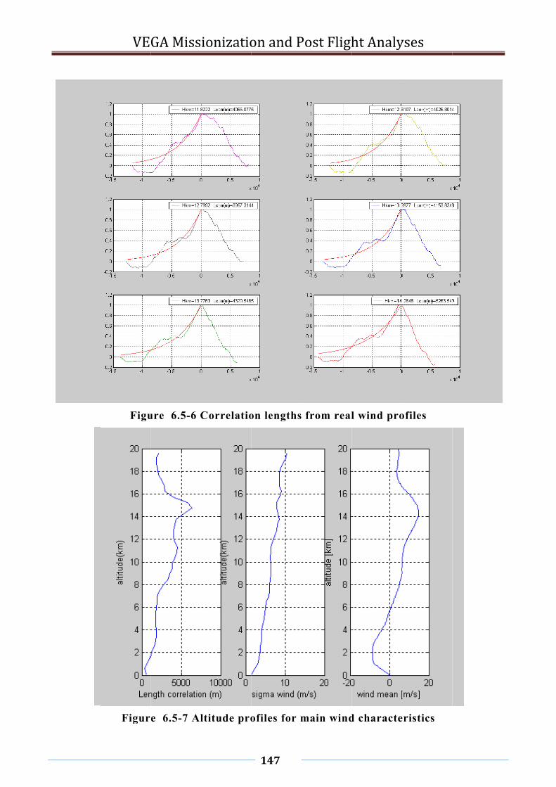
VE
Figu
Figur
GA Miss
ure 6.5-6 C
e 6.5-7 Al
ionizatio
Correlatio
ltitude pro
on and P
147
on lengths
ofiles for m
Post Fligh
from real
main wind
ht Analy
l wind pro
d characte
yses
ofiles
eristics

VEGA Missionization and Post Flight Analyses
148
6.5.5 WIND DYNAMICS CHARACTERIZATION
In this section the characteristics of wind encountered during launch are estimated on the base of a stochastic characterization. In particular the order of the model and correlation times are defined.
The stochastic analysis has been performed on 1000 realisations of wind profiles. These are time profiles of east component of wind at LV CoG from Monte Carlo simulations of DTmin trajectory [RE-01-A5]. Profiles wrt simulation time have been considered because
time constants are required, rather than correlation lengths LV flying throughout frozen altitude profiles of wind is considered variance in LV trajectory related to off-nominal conditions is accounted tool.
In the statistics, value of wind at different simulation times ktx are considered as elements of a
vector x for whom 1000 realisations are available. For each vector, 1500 instants are used corresponding to simulation times between 10 and 70 s, in order to discard regions where wind data is not available nor relevant for simulation (higher altitudes and ground effect).
Covariance is the expected value of the root mean square computed on the base of the 1000 realisations,
jjiiij xExxExEP with ii txx , jj txx and E denoting expected value.
The correlation coefficient jjii
ijij
PP
PC
, computed as the normalized covariance, represents
correlation between values at different instants across the simulation, that is related to causal effects of the Markovian process. Correlation coefficient is presented in Figure 6.5-8 that is a graphical mean to represent the correlation matrix that is symmetric (positive semi-definite), with ones on the diagonal (in the figure rows are sorted according to decreasing simulation time instead of increasing indices, as we are used with matrices). Correlation is bigger for wind values corresponding to close instants since we are not dealing with independent variables, being wind profiles the result of a Markovian process. We do not have constant values on extra-diagonals of the correlation matrix (except for the main diagonal) because the process is non-stationary; this is mostly due to wind characteristics with altitude rather than growing rate of climb.
Figure 6.5-9 reports cross-cuts of the surface reported in Figure 6.5-8 for specific instants with 10 s interval of simulation time, that is the correlation coefficients of a sub-set of elements. As row indices are associated to simulation time, curves have been offset to this value, thus providing profiles that represent correlation as function of shifting in simulation time, that is lag in the correlation. Curves are not symmetric since negative values in abscissa correspond to correlation with wind values in the past, positive time lags are correlation with future values, that would mean anti-causality. Asymmetry is also due to the window of observation, as we have poor information on past at the beginning of the simulation (see the difference of curves related to instants of flights 10 and 60 seconds after lift-off). Remark that in some cases anti-correlation is experienced on long time scales, that can be related to the presence of dominant westward wind near solar tropic (trade-winds) and jet-streams at higher altitudes. Here we focus on the decay of correlation for close times, that is useful to characterize dynamic properties.
Roll-off behaviour of correlation coefficients is regular for all flight instants only when short intervals are considered, where correlations are above 50 %. Outside this range, profiles do not match the exponential decay typical of first order systems, beside the fact that profiles become very sensitive to flight instant. This shows that the criterion mentioned in [RD-25], and also used for PRORA-USV [RD-2], is not applicable. Also remark that for very little intervals the profiles are

VEGA Missionization and Post Flight Analyses
149
rounded as typical of second order systems [RD-25]. This suggests the use of a second order model, though its time constant cannot be extracted from wind profiles here analysed for two main reasons
o Only two mesoscale profiles are implemented in real winds database, therefore correlation on short time scale is not statistically representative
o As this second order phenomenon corresponds to atmospheric turbulence a-posterior implemented in VRC, it is better estimated by means of the turbulence models of Von Karman or Dryden, directly
Figure 6.5-10 presents the profiles of correlation coefficient as function of time shift for all instants of flight. Long scale characteristics are very different wrt instant of flight and are not likely to be represented by a first order model.
Figure 6.5-11 highlights medium and short scales demonstrating that 1st order approximation (with time constant of 10 s)
provides an acceptable fit for medium range, cannot represent the characteristics of a second order model that are noticed for very short
lag in the correlation, that is due to meso-scale turbulence
Characteristic time constant () has been computed assuming a typical first order exponential decay
law for the correlation coefficient, t
ec
. It is ij
iij Tc
T
log considering
only negative lags ( iT <0) in order to discard data concerning correlation to future
a maximum lag of 20 s ( iT >20) to exclude data too far past in the past
corresponding data available for each flight instant (j).
Figure 6.5-12 reports the results of such numerical computation as function of flight time:
o non-stationarity, since time constants (curves) are not invariant wrt flight time (abscissa) o numerical results are affected by the lag at which the computation is performed (different
curves), since profiles are not actually exponential and fitting is not perfect
Nevertheless, on a selected subset, results are similar enough to provide reliable numerical values and statistics were computed on all values in the range 1-10 s of time lag shift (second subplot in Figure 6.5-12).
The time constant for correlation profile is about 10 s during the flight and non-stationarity is not as relevant as shown in the analysis for correlation altitude (par. 6.5.4). This is because both correlation length and rate of climb (RoC) from LV trajectory are increasing with altitude, therefore
transport law makes reduces non-stationarity for correlation time RoC
Lcorr .

VEGA Missionization and Post Flight Analyses
150
Figure 6.5-8 Correlation coefficients of wind values at different instants
Figure 6.5-9 Correlation coefficients as function of time lag
simulation time [s]
correlation coefficient
10 20 30 40 50 6010
20
30
40
50
60
-0.2
-0.1
0
0.1
0.2
0.3
0.4
0.5
0.6
0.7
0.8
-50 -40 -30 -20 -10 0 10 20 30 40 50-0.2
0
0.2
0.4
0.6
0.8
1
time lag [s]
corr
elat
ion
coef
ficie
nt
time correlation profiles at different simulation times
10
20
30
40
50
60
backward correlation
future correlation
sim
time

VEGA Missionization and Post Flight Analyses
151
Figure 6.5-10 Large scale correlation properties
Figure 6.5-11 Medium and short scale fitting of correlation characteristics

VEGA Missionization and Post Flight Analyses
152
Figure 6.5-12 Computation of correlation time constant to address 1st order
0 10 20 30 40 50 60 700
5
10
15
20
25C
orre
latio
n tim
e co
nsta
nt
exponential approximation at different time lags
108.5
7
5.5
4
2.5 1
10 20 30 40 50 60 700
5
10
15
20
25
simulation time [s]
Cor
rela
tion
time
cons
tant
mean
bounds
3 boundssubset

VEGA Missionization and Post Flight Analyses
153
6.5.6 WIND MODEL FOR FILTER
In this section derivation of a suitable Gauss-Markov model for implementation in the Kalman filter is finally described. In particular a time-invariant system was required, corresponding to LV model frozen at a particular condition. This condition corresponds to the region of maximum dynamic pressure, therefore maximum value of A6 parameter, that is the most critical phase for aerodynamic instability. In this condition (at simulation time 57 s)
altitude is 14 km,
LV velocity is 650 m/s,
reference attitude (that is glide-slope being the reference trajectory a gravity turn) is 44°,
therefore rate of climb is 450 m/s.
Wind model is usually approximated with second order models for the purpose of aircraft state estimation. Preliminary modelling and wind dynamics characterization provided information
the reduced Dryden-based model provided two time constant: 0.15 s represents the effect of atmospheric turbulence while a very big value (106) is due to the fact that no information is provided on local winds (this is usually introduced separately for the purpose of wind modelling in simulation environments)
auto-correlation of a single wind profile confirmed the order of magnitude of the meso-scale component of wind but was not sufficient to extract useful information on larger scale, since autocorrelation was computed along the whole time history and a single profile was considered, allowing for no relevant statistical correlation
long scale time constant, estimated on the base of real wind profiles with altitude for launch site, showed a correlation length increasing with altitude with a value about 4000 m for the altitude (14 km) of reference flight condition (57 s); at reference rate of climb it corresponds to 8.87 s correlation time
auto-correlation time constant is confirmed on extensive statistics on real wind database, that also show that non-stationarity is not relevant for correlation times, though it is for correlation lengths
Based on above mentioned time constants, a second order model has been built considering superposition of effects. The model is cast in a form where states are
reduced wind velocity w (that is a contribution to the angle of attack)
reduced wind gradient (that has a physical meaning and can be compared with experimental data before and after flight)
The choice of the states leads to the following form of the state function in continuous time domain, where time constants have been discussed above.
fastslowfastslow TTTT
wA 1111
10
Process noise is introduced on wind gradient. The value of the input matrix is still based on stochastic characterization in order to match a white noise in continuous time. Standard deviation for wind gradient is also normalized to address reduced wind derivative.

VEGA Missionization and Post Flight Analyses
154
Since a discrete time stochastic system was required for implementation, process noise for a discrete time model had to be estimated. The variance of input to turbulence models is usually related to intensity of stationary wind, therefore a series connection was formulated with the fast sub-system fed with the output of the slow sub-model. The variance of the slow system is also derived from statistics on real winds database and is chosen on the base of Figure 6.5-7 and Figure
6.5-3, where a root mean square 10w (m/s) for the reference altitude is selected. This value is
implemented in the input matrix of the system in order to have a normalized white noise as input.
)(010
1111 tref
w
fastslowfastslow Uw
w
TTTTw
w
Eq. 6.5-5 Continuous model for reduced wind
From above mentioned data, the model in Eq. 6.5-5 is defined:
the state is composed by reduced wind and its time derivative
time constants for fast and slow dynamics appear in the state matrix
standard deviation for reduced wind is implemented in the input matrix
The model is transformed into discrete form considering a zero order hold method with the sampling time of major cycle in FPS, that is T4 = 0.040 s. The state matrix for the discrete form is used in assembling the complete model for the filter. Since additive zero-mean process noise is considered, the discrete time model has no input but requires definition of a covariance matrix for process noises. The input matrix is used as baseline definition of the variance of process noise in
discrete form (see Eq. 6.5-6), though this parameter is to be tuned 2tune
heuristically within filter
implementation.
224 ,@0,01,
0,20,01,, tunewd
Twdk
Uwwdwd BBETAdcBA
ref
w
Eq. 6.5-6 Discretization of wind model and variance of process noise

VEGA Missionization and Post Flight Analyses
155
6.6 KALMAN FILTER IMPLEMENTATION FROM SUB-MODELS
In this section the implementation of the Kalman filter for LV wind estimation is described. It consists in assembly of the sub-models described in previous sub-sections and implementation choices. In particular
o the build-up process of a continuous time representation is outlined (par. 6.6.1), o derivation of a discrete time model is then addressed (par. 6.6.2) o stochastic characterization of input to the discrete model (par. 6.6.3) o implementation details are provided at par. 6.6.4.
An overview of the structure of the filter is reported.
Figure 6.6-1 Block diagram for wind estimation filter
6.6.1 DETERMINISTIC CONTINUOUS TIME MODEL
In previous sections, independent models have been described for LV 2dof dynamics, TVC and wind model. These models contribute to definition of the overall filter’s model. The sub-models are defined by the following state and input matrices in deterministic continuous time form.
2
6
3
1
21
66
00
0
0
010
A
AB
UAKB
AUA
AAA wLVLV
22
0
2
00
TVCTVC BA
fastslowfastslow TTTT
wA 1111
10
Ul
CGU
LV 0
001
Eq. 6.6-1 Summary of LV, TVC and wind models
Wind modelGauss-Markov
LV model
2dof rigid bodyTVC model
2nd order
Sensor modelIRS
processnoise
commandednozzle
deflection@T4
outputmeasured
@T4
processnoise
processnoise
measurementnoise

VEGA Missionization and Post Flight Analyses
156
LV sub-model receives input from TVC (actuated nozzle deflection) and wind model (for angle of attack computation). TVC model has commanded deflection as input. Stochastic input are not reported here, they will be applied to the final complete model in discrete form directly.
The output of the complete system are those from LV sub-model.
Stochastic elements are not considered in this model that only represents continuous time deterministic features.
12
2222
12
13
2232
2232
130130
0
00
0
0
00
00x
xxLV
x
TVC
x
wxx
xTVCx
xwBxLVBLV
D
CCBB
A
A
A
A
Eq. 6.6-2 Complete state space model, continuous time deterministic form
The overall representation of the system is reported in Eq. 6.6-2, where matrices are for the continuous time, state space, linear time invariant, normal form, generically described by
uDxCy
uBxAx
Eq. 6.6-3 Typical state space representation in continuous time
The state is the union of states of sub-systems, output are measures from LV IMU and input is the commanded deflection provided by FPS to IPDU, therefore
Twwzqx TIMUIMU zy 0 cmdu
Eq. 6.6-4 Definition of filter’s state, output and input
6.6.2 DISCRETE TIME MODEL FOR FILTER
A discrete time system is more suitable for implementation in digital electronics. This algorithm is aimed at implementation in a fixed step environment with 0.04 s of sample time (25 Hz), that is also the sample of available data: measures and commands.
The discrete form is obtained from the continuous model in closed form solution under the assumptions of linear time invariant system. This avoids implementation of numerical integration and supports integration of the algorithm within stability analyses.
For what concerns input, the commanded deflection is held constant throughout the whole sample period and this correspond to actual behaviour of FPS and IPDU, as explained at par. 0. This corresponds to implementation of a zero-order-hold method, where input is held constant in the integral within Eq. 6.6-5.
t
t
tttt dBuPPetxPPetx0
00 10
1
Eq. 6.6-5 Exact integration of a linear dynamic system
Remark that such discretization is an exact solution for the propagation of the state across the sample period and both effects of nozzle deflection and wind dynamics (input to LV) are properly
represented by means of the internal states ( , , w , w ).

VEGA Missionization and Post Flight Analyses
157
The discrete time normal form for the linear stochastic system is thus obtained from the continuous time representation, in the general form of
kkkk
kkdkdk
vHuDxCy
GuBxAx
1
Eq. 6.6-6 General discrete time representation of linear stochastic systems
It is to be remarked that the only deterministic input to the model is commanded deflection cmdu
and one sample time shift must be implemented in the filter to account for delays in the control loop, as explained in Eq. 6.4-1. This operation is performed within filter implementation because it can be addressed by relative alignment of measures and input alignment, standing the assumption that input delay is exactly one sample period.
6.6.3 STOCHASTIC CHARACTERIZATION (NOISE COVARIANCE)
In this section covariance matrices are defined for
Process noise Measurement noise Initial state
All sub-models have process noises as further input, that are meant to address model uncertainty. They were not considered in the continuous model because it is worthless to define continuous process noise to be integrated with zero order holding or random walks. Process noise is a mean to model uncertainty as further stochastic input and is therefore defined directly on the discrete model.
Forming matrices (H and G) are used to deal with white noise in input. In the Kalman filter we only need covariance matrix Q for noise with no need to specify formal values for H and G, that are necessary to assume normalized noise, instead.
Process noise components are assumed independent as far as no correlation of errors is defined. This makes covariance matrix diagonal and its elements represent uncertainties on each equation of state transition. Variance for each state equation is therefore defined.
The first component addresses uncertainty on propagation of attitude error () that is simply the integral of attitude rate (q) and no uncertainty affects this kinematics relation, therefore a null variance is defined. Variance of attitude error is still affected by propagation of variance of other variables, but this is taken into due account in the equations of Kalman filter and no further stochastic disturbance needs to be introduced.
On the other hand, process noise corresponding to attitude rate and drift velocity are meant to address accuracy of the mathematical model itself. These are tuning parameters but an order of magnitude has been defined as first guess, based on comparison with data from simulations (Table 6.7-1).
Uncertainty on nozzle deflection is modelled with process noise on the transition of its derivative (the 5th state) because TVC dynamics are basically defined in this 5th equation (if we consider this 2nd order system as representative of typical mechanical system, though this is just an approximation of the small loop dynamics). Little process noise is also introduced on the equation of transition of nozzle deflection to support further uncertainties on TVC, both for small loop dynamics (offset, accuracy and quantization) and propulsive forces (misalignment).
Wind sub-model is also affected by uncertainties. A preliminary estimation of variance of the stochastic input to wind model has been derived during its development (par. 0). That value is used

VEGA Missionization and Post Flight Analyses
158
in the complete model as baseline for process noise variance definition. It is introduced concerning
the higher order state ( w ) of wind sub-model in order to provide smoother estimates and
corrections to reduced wind itself. The baseline value is though scaled by a factor tuned empirically as the main driver for filter performance.
Covariance matrix for measurement noise has been defined by sensor characterization at par. 0.
Initial condition for the filter state can be set at zero, that is not too far from reference nominal conditions. Only nozzle deflection is assigned a value from previous step command in order to match possible trim values according to the region of flight considered, in particular because this value is available.
Initial condition for state covariance matrix is not of great concern because stationary solution of covariance is reached very fast, as it is shown in Figure 6.8-4.
6.6.4 FILTER IMPLEMENTATION
The environment for Kalman filtering follows these phases:
a) Model configuration
b) Data loading and pre-processing
c) Tuning of filter parameters
d) Filter model preparation
e) Filtering execution
f) Post processing
In the first step basic options are defined. For instance the instant of nominal simulation from which data have to be gathered for LV model definition, in case of frozen time approach. Wind model selection was a further option in the preliminary phase, where wind model characterization was an open issue. Furthermore uncertainties on LV model parameter can be introduced.
Next the simulation from which data are loaded is selected, allowing for testing several simulations with different wind profiles. Measurements and commands are collected to be fed to the filter. The exact solution is also computed to be compared with filter estimates of state and output, in particular to verify the accuracy of wind estimation wrt simulated wind (true values).
Another preliminary operation is tuning of filter’s parameters, in particular variances of process noises. Initial conditions are also set for estimated state and covariance.
Filter model preparation consists of building the sub-models, inter-connecting them to form a unique continuous time model, discretization, as described in previous sub-sections. Data for LV parameters are loaded from a dedicated nominal simulation with no wind, where time profiles of LV parameters are computed. Covariance of process noise is further corrected according to selected sub-models.
All above mentioned operations can be performed a-priori and are not to be considered within the budget of on-line computation time. This procedure address filter design and tuning in the development phase. Also Kalman gain can be computed a-priori using the closed form solution of the Riccati equation (par. 4.3). This is suggested not only to save on-line computation time, but to make Kalman gain a-priori defined therefore allowing stability analyses of the closed loop system including the estimation algorithm. Remark that implementation of a time scheduled filter requires loading data for Kalman gain instead of process and measurements noise covariance matrices. Nevertheless, in these applications, Kalman gain is computed recursively during filtering because
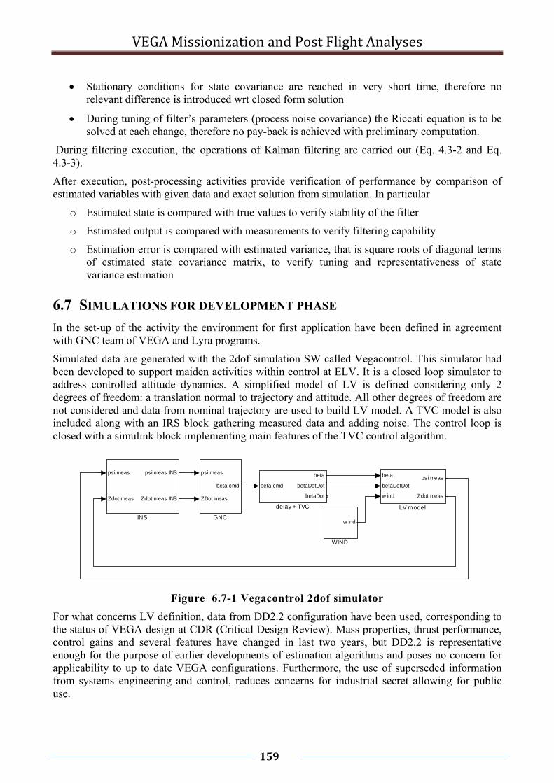
VEGA Missionization and Post Flight Analyses
159
Stationary conditions for state covariance are reached in very short time, therefore no relevant difference is introduced wrt closed form solution
During tuning of filter’s parameters (process noise covariance) the Riccati equation is to be solved at each change, therefore no pay-back is achieved with preliminary computation.
During filtering execution, the operations of Kalman filtering are carried out (Eq. 4.3-2 and Eq. 4.3-3).
After execution, post-processing activities provide verification of performance by comparison of estimated variables with given data and exact solution from simulation. In particular
o Estimated state is compared with true values to verify stability of the filter
o Estimated output is compared with measurements to verify filtering capability
o Estimation error is compared with estimated variance, that is square roots of diagonal terms of estimated state covariance matrix, to verify tuning and representativeness of state variance estimation
6.7 SIMULATIONS FOR DEVELOPMENT PHASE
In the set-up of the activity the environment for first application have been defined in agreement with GNC team of VEGA and Lyra programs.
Simulated data are generated with the 2dof simulation SW called Vegacontrol. This simulator had been developed to support maiden activities within control at ELV. It is a closed loop simulator to address controlled attitude dynamics. A simplified model of LV is defined considering only 2 degrees of freedom: a translation normal to trajectory and attitude. All other degrees of freedom are not considered and data from nominal trajectory are used to build LV model. A TVC model is also included along with an IRS block gathering measured data and adding noise. The control loop is closed with a simulink block implementing main features of the TVC control algorithm.
Figure 6.7-1 Vegacontrol 2dof simulator
For what concerns LV definition, data from DD2.2 configuration have been used, corresponding to the status of VEGA design at CDR (Critical Design Review). Mass properties, thrust performance, control gains and several features have changed in last two years, but DD2.2 is representative enough for the purpose of earlier developments of estimation algorithms and poses no concern for applicability to up to date VEGA configurations. Furthermore, the use of superseded information from systems engineering and control, reduces concerns for industrial secret allowing for public use.
beta cmd
beta
betaDotDot
betaDot
delay + TVC
w ind
WIND
beta
betaDotDot
w ind
psi meas
Zdot meas
LV m odel
psi meas
Zdot meas
psi meas INS
Zdot meas INS
INS
psi meas
ZDot meas
beta cmd
GNC

VEGA Missionization and Post Flight Analyses
160
Time profiles of nominal trajectory correspond to the Reference trajectory for VEGA design, that is a polar azimuth with circular final orbit at 700 km. The reference PL for this mission is 1500 kg. Nominal data to define the reference trajectory are therefore computed on the base of a typical VEGA mission, centred within the performance map of PL mass from 300 to 2500 kg and orbits between 300 and 1500 km. Time profiles of pitch program, dynamic pressure, thrust and Mach number are presented in Figure 6.7-2.
Reference trajectory is used to build the model but is not a constraint for Vegacontrol 2dof simulator. According to this a lighter PL mass has been implemented in simulations, that is the lowest in the performance map (300 kg) thus providing higher sensitivity to wind perturbations.
For what concerns wind profile, data from a real wind have been introduced in order to provide the most realistic scenario for estimation. This wind profile has been selected as the most critical for the driving parameter for general loads [NT-204], that is the product of dynamic pressure and angle of attack. This wind profile is extracted from real wind database (par. 6.5.3). The choice is motivated by the interest of providing improvements in wind estimation with particular concern for critical cases. In particular the east component of such wind profile is addressed, as it presents the most critical characteristics, that is a strong gradient for a long period (Figure 6.7-4). Further wind profiles have been used to address different aspects:
No wind, to provide reference values and build nominal LV model
East component of wind at midnight of 28.02.1998, the most critical for loading, due to a relevant ramp increase in the region of highest dynamic pressure, outside 99% envelopes of long scale gradient [ST-08] implemented in synthetic winds
North component of the same wind, presents small high frequency oscillations (turbulence)
Synthetic wind with gust of square profile in the region of maximum dynamic pressure (15 km of altitude), a typical profile for control tuning also used in literature for LV control
Wind profiles wrt altitude are assumed to be frozen during the first stage simulation and horizontal in the trajectory plane (a plane defined by local vertical and azimuth). The time profile is obtained through altitude profile of LV in reference trajectory according to transport assumption. Wind is also projected according to reference profile of pitch to provide the component normal to trajectory. The longitudinal component is not addressed in the 2dof application. For the purpose of preliminary evaluation of performance, a single instant flight path is considered, that is equal to pitch attitude in a gravity turn trajectory. Resulting time profiles are shown in Figure 6.7-4.
LV model is frozen at values corresponding to 57 s of simulation time, that is the instant of maximum dynamic pressure. This is the most critical point for stability since aerodynamic instability (A6 coefficient) reaches its maximum value. Therefore a LTI system is addressed. Further dynamics are not included, that is bending, sloshing, TWD effect and uncertainties are not implemented, thus providing results for nominal LV. Time profiles of most relevant coefficients are presented in Figure 6.7-3.
LV and IRS model are based on continuous time formulations discussed in par. 6.2 and 0. Random noise with appropriate variance is added to LV output to represent IRS disturbance.
TVC model is basically the one introduced at par. 0, including rate saturation effect.
Control system is represented by a transport delay of 40 ms and discrete time filters running at 25 Hz with control gains according to the architecture of TVC algorithms within VEGA FPS [DF-07].
The highest level of blocks is reported in Figure 6.7-1.
Time profiles of most relevant variables is shown in Figure 6.7-5 and Figure 6.8-1.

VEGA Missionization and Post Flight Analyses
161
Filter’s model is a fair representation of simulation model (or vice versa) apart from wind dynamics. Nevertheless differences can arise from numerical integration since a variable step solver is implemented for simulations while discrete time model is chosen for the filter. Further preliminary activities have been carried out on modeling before implementing the final filter.
Preliminary values for variance of process noises have been derived from evaluation of filter’s model and simulated profiles. Table 6.7-1 collets order of magnitudes of several reference variables, gathered from empirical analysis of time profiles for each state variable.
o Most relevant addendums in each equation are a reference value for the required order of magnitude of a correcting term (ith addendum is not considered in ith state because it is near to unity)
o All together they provide the order of magnitude of the variable itself
o A useful evaluation of the error to be accounted for with filter’s model is computed by comparison of
the increment of states across sample period from simulation (where a variable step solver was used for integration) and
filter’s model fed with previous sample of true state. The value of the increment across sample period gives the order of magnitude of the correction term.
Based on engineering judging of these values and assumptions, baseline values are found for process noise.
Order of magnitude of reference elements
state single terms in equation of transition
Total of equation of transition
Error of state propagation
State increment in
sample period
Baseline variance of process noise
1,0E-03 1,0E-02 1,0E-05 5,0E-04 0
q 1,0E-02 1,0E-02 1,0E-03 1,0E-03 0,3 x 10⁻⁶
0 1,0E-04 5,0E-03 5,0E-05 5,0E-04 50 x 10-6
1,0E-01 1,0E-02 5,0E-06 1,0E-03 0
' 1,0E-02 3,0E-02 1,0E-03 5,0E-02 0,1 x 10⁻³
w 1,0E-01 5,0E-02 1,0E-02 1,0E-03 0
w' 1,0E-02 1,0E-02 1,0E-02 1,0E-02 7,96 x 10⁻³
Table 6.7-1 Choice of reference order of magnitude for state function error

VEGA Missionization and Post Flight Analyses
162
Figure 6.7-2 Time profiles of reference trajectory
Figure 6.7-3 Main stability and control derivatives
0 50 10020
40
60
80
100
simulation time [s]
pitc
h [d
eg]
0 50 1000
2
4
6x 10
4
simulation time [s]
Pdy
n [P
a]
0 50 1000
1
2
3x 10
6
simulation time [s]
Thr
ust
[N]
0 50 1000
2
4
6
simulation time [s]
Mac
h
0 10 20 30 40 50 60 70 80 900
1
2
3
4
A6
0 10 20 30 40 50 60 70 80 900
5
10
15
K1
simulation time [s]
non-stationary LV model
LV frozen at 57 s

VEGA Missionization and Post Flight Analyses
163
Figure 6.7-4 Wind profiles for 2dof simulations
0 10 20 30 40 50 60 70 80 90-10
0
10
20
30
40
50
60
simulation time [s]
win
d sp
eed
[m/s
], n
orm
al t
o tr
ajec
tory
Real wind: East component
real wind: North componentSynthetic wind

VEGA Missionization and Post Flight Analyses
164
Figure 6.7-5 Time profiles of attitude error, incidence and nozzle deflection, for non-stationary LV model, the frozen time model and nominal conditions without wind
0 10 20 30 40 50 60 70 80-2
-1
0
1
2
3
[d
eg]
0 10 20 30 40 50 60 70 80-5
0
5
[
deg]
0 10 20 30 40 50 60 70 80-3
-2
-1
0
1
2
[d
eg]
simulation time [s]
non-stationary LV model
LV frozen at 57 snominal no-wind

VEGA Missionization and Post Flight Analyses
165
6.8 RESULTS IN NOMINAL CONDITIONS
The Kalman filter for wind estimation has been applied to a nominal 2dof simulation, therefore neglecting high frequency dynamics and LV uncertainties. This is to address performance but not robustness, that is evaluated in par. 6.9.
Figure 6.8-1 shows time profiles of several variables representing LV dynamics. They address different features of the simulation but are reported all together to provide understanding of the situation. As mentioned variables are normalized and, since they basically represent angles, they all have comparable orders of magnitude.
Wind induced angle of attack (w) that is the reduced wind, is an input to the 2dof simulation and matches the profile shown in Figure 6.7-4 for east component of the selected real wind profile: after slow varying profile (up to 40 s) and small oscillations (before 60 s), a strong gradient is encountered.
TVC deflection () is affected by noise resulting from IRS measures and also copes with wind dynamics in order to counteract such disturbance, both for small oscillations and the constant rate region.
TVC control is particularly effective in stabilizing attitude error () that is affected by wind disturbance. Remark that under strong wind gradient attitude error is almost zero.
Drift velocity 0 (wrt nominal trajectory and reduced with LV speed) is characterized by
smaller low frequency dynamics. In particular we notice that it follows wind in a smoothed and delayed fashion. In the region at constant wind gradient, lift is linearly growing and drift velocity has a parabolic profile, as normal acceleration roughly corresponds to lift.
Angle of attack w 0 is composed by attitude error, reduced drift and reduced
wind. After 60 s, attitude is stabilized near zero, drift is negligible and angle of attack is approximated by the opposite of reduced wind.
Output and measures. Figure 6.8-2 presents filter’s output and corresponding measurements showing that Kalman filter fits available measurements reducing stochastic dispersion, since information on LV dynamics is used along with noisy measurements.
State variables. Figure 6.8-3 provides time profiles of estimated states along with actual values retrieved from simulation. Nozzle deflection is not presented here as it basically follows given TVC commands. Time derivatives of nozzle deflection and angle of attack are not reported either. LV states and estimated wind are concerned. Perturbations of attitude (that is attitude error, since reference trajectory corresponds to commanded pitch) and perturbation of flight path angle (that is drift velocity normal to trajectory divided by LV speed) are particularly accurate because these variables are almost directly measured, as shown in previous figure. Reduced wind, that is the contribution to angle of attack, is estimated with remarkable accuracy, though it appears slightly noisy and presents a little delay in the region of constant wind gradient. Attitude rate estimation only presents relevant error wrt true value of the state where wind gradient changes sign abruptly.
Estimation errors. Figure 6.8-4 better highlights estimation errors (difference of estimated states and respective values in the simulation) and compares them with estimated standard deviation. The latter is computed as squared root of diagonal elements of the estimated covariance matrix, not considering correlation of states. These can be considered as estimated errors by the filter, though their stochastic dispersion is actually addressed in a Kalman filter and it is not a reliable mean of assessing filter’s performance. Nevertheless the fact that process noise leads to a stationary solution

VEGA Missionization and Post Flight Analyses
166
for state covariance having the same order of magnitude of estimation error confirms that proper tuning has been found for filter’s parameters. This is rather a cause than an effect of performance.
Comparison with Ariane. These results are compared with corresponding wind estimation on Ariane launcher [GNC-A5]. Figure 6.8-5 reports estimated and actual wind profile where a synthetic profile with gust at 15 km had been used. Wind estimation is quite accurate apart from last region of flight, where dynamic pressure drops (and so aerodynamic parameter A6) reducing wind identifiability and observability. Figure 6.8-6 reports results of the present application showing higher performance, though it is to be reminded that a stationary nominal simulation is here considered. As different launchers are addressed, time profiles are different; in particular VEGA first stage is faster and reaches altitude of 15 km at 55 s, where Ariane 4 gets at 90 s.
Angle of attack. Figure 6.8-7 presents estimation profiles of angle of attack, that is another aspect of the problem of wind estimation, more related to LV dynamics and control. Estimation for Ariane 4 appears less accurate with both an offset error and a delay, compared to results here attained.
Performance with any wind profile. Filter’s performance has been proved on different wind profiles in order to assess its extension to any simulation. Wind estimation has been carried out with the same values for design and tuning parameter but different sets of data in input; this is to say that no filter re-tuning is allowed for adaptation, as design phase is considered concluded and validation is here addressed. Data correspond to the simulations presented in par. 6.7 and wind profiles shown in Figure 6.7-4. Estimation of LV states is basically equivalent for the different profiles. Figure 6.8-8 summarizes estimated and actual profiles of wind and angle of attack. Performance is quite similar despite different characteristics of wind dynamics are addressed: small high frequency oscillations, strong gradient, increasing gradient with trapezoidal gust. Estimation performance is always very high, only in case of abrupt changes is lost. This is the case for inversion of wind gradient that occurs at 65 s with east component of real wind and trapezoidal gust in synthetic wind case. Remark that this behaviour is not properly modelled in the 2nd order wind model because it is not likely to occur. As a matter of fact a rare profile has been considered among real wind database and an ideal non physical gust is implemented with synthetic wind.

VEGA Missionization and Post Flight Analyses
167
Figure 6.8-1 Time profiles of variables from simulation
Figure 6.8-2 Filtering of measurements
0 10 20 30 40 50 60 70 80-5
-4
-3
-2
-1
0
1
2
3
4
5Comparison of several angles [deg]
[deg]
0 [deg]
w [deg]
0 10 20 30 40 50 60 70 80 90-1
0
1
2
3
4
mea
s
Measurement filtering
data
estim
0 10 20 30 40 50 60 70 80 90-2
0
2
4
6
v mea
s
Measurement filtering
data
estim

VEGA Missionization and Post Flight Analyses
168
Figure 6.8-3 State estimation performance profiles
Figure 6.8-4 Estimation error and estimated error
0 10 20 30 40 50 60 70 80
0
1
2
3
[d
eg]
Perturbation of Attitude angle [deg]
estim
true
0 10 20 30 40 50 60 70 80
00.20.4
0 [
deg]
Perturbation of flight path angle [deg]
estim
true
0 10 20 30 40 50 60 70 80
0
2
4
w
[de
g]
- Wind induced Angle of attack [deg]
estim
true
0 10 20 30 40 50 60 70 80-2
0
2
q [d
eg/s
]
Attitude rate [deg/s]
estim
true
0 20 40 60 80
-0.06
-0.04
-0.02
0
0.02
0.04
(
[de
g])
estimation errors
0 20 40 60 80
-10
-5
0
5
x 10-3
(
0 [de
g])
estimation errors
0 20 40 60 80
-0.5
0
0.5
1
(
w [
deg]
)
estimation errors
0 20 40 60 80
-0.6
-0.4
-0.2
0
0.2
(q
[de
g/s]
)
estimation errors
error
est.

VEGA Missionization and Post Flight Analyses
169
Figure 6.8-5 Wind estimation in Ariane
Figure 6.8-6 Estimated and actual wind
0 20 40 60 80-10
0
10
20
30
40
50
60Wind component [m/s] normal to trajectory
estim
true

VEGA Missionization and Post Flight Analyses
170
Figure 6.8-7 Accuracy in estimation of aerodynamic incidence
Figure 6.8-8 Estimation of wind and incidence with different wind profiles
0 10 20 30 40 50 60 70 80 90-6
-4
-2
0
2
4
[
deg]
estim
true
0 10 20 30 40 50 60 70 80 90-6
-4
-2
0
2
4
[
deg]
Angle of attack for different wind profiles
Wind North
simulated
Wind Eastsimulated
Synthetic
0 10 20 30 40 50 60 70 80 90-40
-20
0
20
40
60Wind component [m/s] normal to trajectory
Wind North
simulated
Wind Eastsimulated
Synthetic

VEGA Missionization and Post Flight Analyses
171
6.9 ROBUSTNESS TO UNCERTAINTIES
The subject of model uncertainty is here addressed, that is particularly critical for stochastic filtering because deterministic errors are not corrected and induce estimation errors. Estimation errors are beyond model inaccuracy and are caused by the optimization criterion, as effects of modeling errors are erroneously compensated throughout state estimates. Several sources of uncertainty make LV parameters not exactly known, introducing a relevant uncertainty in filter’s model. This is a very demanding problem for VEGA GNC design and validation.
Loss of performance is shown with following examples:
100 Monte Carlo runs introducing an error on all coefficients of LV model; this random uncorrelated error has normal distribution with 3 level corresponding to 25% of each parameter;
Percent error on A6 parameter; this is a more realistic scenario of uncertainty;
The first case is used to evaluate general robustness of the algorithm to model uncertainties. All parameters concerning LV are perturbed randomly and independently. Figure 6.9-1 shows that wind estimation is affected by model uncertainty, as known for Kalman filters, though we never experience divergence of the solution. State estimation preserves very good accuracy, therefore only wind estimation is affected but uncertainty do not degrade estimation of LV motion (Figure 6.9-2). This robustness is mainly due to the fact that most LV output are measured and its state is observable, despite loss of accuracy of dynamic model. Estimation error (Figure 6.9-3) is affected for wind and angle of attack estimation, not for attitude and drift states.
LV parameters are not all independent, as we find in Eq. 6.2-4. The parameter A6 (the most important for short period dynamics) appears in three different terms, wherever angle of attack is concerned. A more realistic condition of uncertainty is given by off-nominal value for this parameter, considering its effects on LV model. Uncertainties of A6 are basically driven by dynamic pressure, that is strongly affected by thrust uncertainties. MCI and aerodynamic properties also affect A6.
Wind estimation with some settings for A6 error are presented in Figure 6.9-4. Underestimation of A6 results particularly dramatic because, as a result, wind is over-estimated.
Other LV states are not sensibly affected by model error (Figure 6.9-5).
These studies suggest that the filter is quite robust to model uncertainties, though their effect limits its performance for wind estimation. Augmenting process noise on wind often improves its estimation but LV states are negatively affected.
Nevertheless these results are acceptable from the point of view of integration within GNC algorithms because
Needs for control verification have been duly addressed Estimation of angle of attack always provides a rough information to support evaluation of
aerodynamic loading Estimation can support control laws based on knowledge of aerodynamic angles, despite the
lack of measurements As LV states are accurate even in worst scenarios of model uncertainties, providing and
smoothed estimates of vehicle motion, these could be used to provide control algorithms with filtered input not affected by measurement noise and bending action, thus reducing the need for complex filters within control algorithms.

VEGA Missionization and Post Flight Analyses
172
These results suggest future investigation concerning performance improvements with alternative developments for both navigation algorithms (Kalman filters for state observation and wind estimation) and control (integrated with improved navigation algorithms).
Figure 6.9-1 Wind estimation with 25% error on LV parameters
Figure 6.9-2 State estimation with 25% uncorrelated random errors
0 10 20 30 40 50 60 70 80 90-20
0
20
40
60
80
100Wind component [m/s] normal to trajectory
nominal
true
25% random error on LV model parameters
0 10 20 30 40 50 60 70 80-10
1
2
3
[d
eg]
Perturbation of Attitude angle [deg]
0 10 20 30 40 50 60 70 80
00.20.4
0 [
deg]
Perturbation of flight path angle [deg]
0 10 20 30 40 50 60 70 80
0
2
4
w
[de
g]
- Wind induced Angle of attack [deg]
0 10 20 30 40 50 60 70 80-2
0
2
q [d
eg/s
]
Attitude rate [deg/s]
estim
true
estim
true
estim
true
estim
true

VEGA Missionization and Post Flight Analyses
173
Figure 6.9-3 Estimation error with 25 % uncorrelated random errors on LV
Figure 6.9-4 Wind estimation in case of error in A6 for LV model for filter
0 20 40 60 80
-0.06
-0.04
-0.02
0
0.02
0.04
(
[de
g])
estimation errors
0 20 40 60 80
-10
-5
0
5
x 10-3
(
0 [de
g])
estimation errors
0 20 40 60 80
-0.4
-0.2
0
0.2
0.4
0.6
0.8
(
w [
deg]
)
estimation errors
0 20 40 60 80
-0.6
-0.4
-0.2
0
0.2
(q
[de
g/s]
)
estimation errors
error
est.
0 10 20 30 40 50 60 70 80 90-20
0
20
40
60
80
100
120Wind component [m/s] normal to trajectory
nominal
true-10% A
6
true
+10% A6
true
-50% A6
true
+50% A6

VEGA Missionization and Post Flight Analyses
174
Figure 6.9-5 State estimation in case of errors on A6 filter’s model
0 10 20 30 40 50 60 70 80-1
0
1
2
3
[deg
]
Perturbation of Attitude angle [deg]
0 10 20 30 40 50 60 70 80
0
0.2
0.4
0 [
deg]
Perturbation of flight path angle [deg]
0 10 20 30 40 50 60 70 80-202468
w
[de
g]
- Wind induced Angle of attack [deg]
58 60 62 64 66 68 70-2
0
2
q [d
eg/s
]
Attitude rate [deg/s]
estim
true
estim
true
estim
true
estim
true

VEGA Missionization and Post Flight Analyses
175
7 CONCLUSIONS
This work addressed several main subjects
VEGA Missionization Non-linear systems identification Recursive real time wind estimation Activities within VEGA qualification
VEGA missionization dealt with systems engineering and consisted in organizing procedures to manage all activities necessary to prepare a launch. The main results consisted in
Definition of the missionization plan and ELV document [PL-28] Support to development of a software to implement functionalities required by
missionization plan and systems engineering database
Beside VEGA missionization with ELV, research in the field of non-linear systems identification has been carried out in the frame of PRORA-USV in co-operation with CIRA. Methodologies and algorithms have been developed to address the problem of post flight analysis of an experimental re-entry vehicle. Non-linear identification mainly focused on estimation/correction of the aerodynamic model in transonic regime. In this work
o architectures of the whole systems identification procedures have been developed and discussed; in particular the estimation before modelling approach was addressed with recursive non linear techniques, in the frame of filtering approach methods and stochastic modelling
o the technique of the Unscented Kalman Filter has been deeply studied and applied with several variation in its implementation and set-up of the Unscented Transformation
o an analytical model based on physical insights have been introduced to describe vehicle aerodynamics across all regimes of mach, with particular concern on transonic
Results consisted in
methodological developments based on simulated data of DTFT 1 mission; delivery of [D1.1 PI], [D1.3 PI], [D2.1 PI], [D2.2 PI] and presentation at AIAA Atmospheric Flight Mechanics conference [RD-1]
modification of the architecture for systems identification and adaptation to specific constraints of available flight data of DTFT 1; support to application to flight data with successful correction of aerodynamic database of FTB (results presented at IFAC symposium [RD-2])
support to CIRA for application to simulated data of DTFT 2, also addressing turn manoeuvres with publication on Journal of Aircraft [RD-3]
Methodologies developed for CIRA USV are suitable for application to VEGA in post flight analyses, though dedicated modelling is required to adapt the general approach and address further issues that are inherent to launch vehicle and not encountered with FTB. Nevertheless, in this work, the research at ELV for VEGA was oriented on the problem of wind estimation on board.
Linear Kalman filtering has been applied due to strong constraints from the control team and the need of a higher technology readiness level. The most relevant results are
application of wind estimation by recursive stochastic filtering dedicated to real time on-board VEGA computer, addressing all constraints from VEGA avionics and GNC validation process
great accuracy in nominal conditions and acceptable in very demanding off-nominal cases

VEGA Missionization and Post Flight Analyses
176
feasibility for implementation within navigation algorithms to support control
Several analysis activities have also been carried out within VEGA qualification concerning different subjects
thrust vectoring control actuation modelling and effects for GNC Monte Carlo analysis of sizing parameters Effects of structural dynamics coupling with closed loop control Updating of VEGA simulator and support to control tuning for VEGA qualification review
Results are reported in documents delivered at ELV:
P80 TVC SWIL model impacts on GNC [NT-113]
AVUM TVC SWIL impacts on GNC [NT-1447]
Identification of uncertainties for parameters of 2nd order TVC model [NI-264]
Dispersed trajectories for design [NT-168]
GNC analyses for PL loading [NT-289]
Test plan and test reports of control tuning for DD3.1 LV configuration (to be issued)
All these works supported VEGA qualification and were addressed considering implications with VEGA program and missionization from a higher point of view. GNC improvements have been suggested to cope with engineering problems detected.
Future work in VEGA program has been motivated by results presented within this PhD:
Post flight analyses of VEGA telemetry flight data with organization of all related activities Improvements for VEGA FPS considering implementation of navigation algorithms to
support control with on-board estimated variables (e.g. angle of attack)

VEGA Missionization and Post Flight Analyses
177
8 ANNEXES
8.1 ANNEX A - MISSIONIZATION GRAPHS
Some views of the graph implemented for missionization are here presented. The overall process is described by a complex graph whose elements have been ordered as to provide an idea of logical flow chart and time sequence when read from left to right. The overall graph is split in 2 figures for the sake of readability (Figure 8.1-1 and Figure 8.1-2). Main phases are extracted and presented in next figures (Figure 8.1-3, Figure 8.1-4 and Figure 8.1-5). Figure 8.1-6 presents a view with time markers focusing on the launch preparation phase.
Figure 8.1-1 Overall missionization graph, left side
Figure 8.1-2 Overall missionization graph, right side

VEGA Missionization and Post Flight Analyses
178
Figure 8.1-3 Preliminary Analyses Phase MPh.2
Figure 8.1-4 Final Analyses Phase MPh.3

VEGA Missionization and Post Flight Analyses
179
Figure 8.1-5 Production and integration phase MPh.4

VEGA Miss
Figure 8
ionizatio
.1-6 Graph
on and P
180
hical Sche
Post Fligh
edule with
ht Analy
h timelines
yses
s

VEGA Missionization and Post Flight Analyses
181
8.2 ANNEX B – MATHEMATICAL MODELLING OF LAUNCH VEHICLE
DYNAMICS
Figure 8.2-1 Definitions for LV modelling
The general expression of equilibrium equation is
Eq. 8.2-1 Equations of motion for rigid body mechanics
Assuming symmetry of LV and motion in a single plane of symmetry, Eq. 8.2-1 are specialized in Eq. 8.2-2
Eq. 8.2-2 Equations in 3 dof standing LV axial-symmetry
Expression of forces and moments include aerodynamics, propulsion and gravity. Thrust is vectored by TVC control of nozzle. Aerodynamics are defined by drag and lift and center of effort and a linear expression is assumed for lift wrt angle of attack. Trajectory reference frame is assumed locally coincident with body reference frame, since very small angle of attack are to be accounted for.

VEGA Missionization and Post Flight Analyses
182
Eq. 8.2-3 Expression of forces and moment on LV
Eq. 8.2-4 Equations of motion in 3 dof
Eq. 8.2-5 Equations of motion in normal form


![Flight Test and Analyses of the B·1 StrlJcttural Mode Control … · 2013-08-31 · 1 1] NASA Contractor RE~port 170405 NASA-CR-170405 19840005129 Flight Test and Analyses of the](https://img.pdfslide.net/doc/110x75/5e98244bcdb8cb0c9e717e98/flight-test-and-analyses-of-the-b1-strljcttural-mode-control-2013-08-31-1-1-nasa.jpg)