Vekua theory for the Helmholtz operator - CentAURcentaur.reading.ac.uk/28022/2/Vekua-Zamp-Final.pdfVekua theory for the Helmholtz operator 3 We conclude this introduction by ﬁxing

Vekua theory for the Helmholtz operator Article

Accepted Version

Moiola, A., Hiptmair, R. and Perugia, I. (2011) Vekua theory for the Helmholtz operator. Zeitschrift für Angewandte Mathematik und Physik, 62 (5). pp. 779807. ISSN 00442275 doi: https://doi.org/10.1007/s0003301101423 Available at http://centaur.reading.ac.uk/28022/

It is advisable to refer to the publisher’s version if you intend to cite from the work. See Guidance on citing .

To link to this article DOI: http://dx.doi.org/10.1007/s0003301101423

Publisher: Springer

All outputs in CentAUR are protected by Intellectual Property Rights law, including copyright law. Copyright and IPR is retained by the creators or other copyright holders. Terms and conditions for use of this material are defined in the End User Agreement .

www.reading.ac.uk/centaur

CentAUR

Central Archive at the University of Reading

Reading’s research outputs online

http://centaur.reading.ac.uk/71187/10/CentAUR%20citing%20guide.pdf

http://www.reading.ac.uk/centaur

http://centaur.reading.ac.uk/licence

Vekua theory for the Helmholtz operator

A. Moiola, R. Hiptmair and I. Perugia

Abstract. Vekua1 operators map harmonic functions defined on domain in R2 to solutions of elliptic

partial differential equations on the same domain and vice versa. In this paper, following the originalwork of I. Vekua, we define Vekua operators in the case of the Helmholtz equation in a completelyexplicit fashion, in any space dimension N ≥ 2. We prove i) that they actually transform harmonicfunctions and Helmholtz solutions into each other; ii) that they are inverse to each other; iii) thatthey are continuous in any Sobolev norm in star-shaped Lipschitz domains.

Finally, we define and compute the generalized harmonic polynomials as the Vekua transformsof harmonic polynomials. These results are instrumental in proving approximation estimates forsolutions of the Helmholtz equation in spaces of circular, spherical and plane waves.

Mathematics Subject Classification (2010). 35C15, 35J05.

Keywords. Vekua transform, Helmholtz equation, generalized harmonic polynomials, Sobolev con-tinuity.

1. Introduction and Motivation

Vekua’s theory (see [20, 36]) is a tool for linking properties of harmonic functions (solutions of theLaplace equation ∆u = 0) to solutions of general second-order elliptic PDEs Lu = 0: the so-calledVekua operators (inverses of each other) map harmonic functions to solutions of Lu = 0 and viceversa.

The original formulation targets elliptic PDEs with analytic coefficients in two space dimensions.Some generalizations to higher space dimensions have been attempted, see [10–12, 18, 23, 24] and thereferences therein, but the Vekua operators in these general cases are not completely explicit.

Here, the PDE we are interested in is the homogeneous Helmholtz equation Lu := ∆u+ω2u = 0.In this particular case, simple explicit integral operators have been defined in the original work of Vekuain any space dimension N ≥ 2 (see [34, 35], [36, p. 59], and Fig. 1), but no proofs of their propertiesare provided and, to the best of our knowledge, these results have been used later on only in very fewcases [9, 25].

Vekua’s theory has surprising relevance for numerical analysis. Several finite element methodsused in the numerical discretization of the Helmholtz equation ∆u+ω2u = 0 are based on incorporatinga priori knowledge about the differential equation into the local approximation spaces by using Trefftz-type basis functions, namely functions which belong to the kernel of the Helmholtz operator.

Examples of methods using local approximating spaces spanned by plane wave functions x 7→eiωx·d, d ∈ SN−1, are the Plane Wave Partition of Unit Method (see, [4]), the Ultra Weak VariationalFormulation (see [8]), the Plane Wave Least Squares Method (see [32]), the Discontinuous EnrichmentMethod (see [16]), and the Plane Wave Discontinuous Galerkin Method (see [19, 22]). Other methodsare based on generalized harmonic polynomials (Fourier-Bessel functions), like the Partition of Unit

1Ilja Vekua (1907-1977), Soviet-Georgian mathematician

2 A. Moiola, R. Hiptmair and I. Perugia

. . .

Figure 1. Two paragraphs of Vekua’s book [36] addressing the theory for the Helm-holtz equation

Method of [29], the version of the Least Squares Method presented again in [32] and the method of [6],or on Hankel functions, like the Method of Fundamental Solutions of [5].

The convergence analysis of each of these techniques requires best approximation estimates : thefinite element space must contain a function which approximates the analytic solution of the problemwith an error that tends to zero when the mesh size h is reduced (h-convergence), or when thedimension p of the local approximating space is raised (p-convergence). This error is usually measuredin Sobolev norms and an explicit estimation of the convergence rate with respect to the parameters hand p is very desirable.

In the case of plane waves, only few approximation estimates are available in the literature. Afirst one is contained in Theorem 3.7 of [8]: the proof was based on Taylor expansion and only h–convergence for two-dimensional domains was proved; moreover, the obtained order of convergenceis not sharp. A more sophisticated result is Proposition 8.4.14 of [27]: in this case, p–estimates wereobtained in the two-dimensional case by using complex analysis techniques and Vekua’s theory. Asimilar approach was used in [30] to prove sharp estimates in h for the PWDG method in 2D; there,the dependence on the wave number was made explicit. In order to generalize and make precise theresults of [27] and [30], it is necessary to study in more details the basic tool used: Vekua’s theory. Thispaper is devoted to this purpose: the results developed here will be the main ingredients in the proofof best approximation estimates by circular, spherical and plane waves. This has been done in [21]and greately improved in [31].

We proceed as follows: in Section 2, we will start by defining the Vekua operators for the Helm-holtz equation with N ≥ 2 and prove their basic properties, namely, that they are inverse to eachother and map harmonic functions to solutions of the homogeneous Helmholtz equation and vice versa(see Theorem 2.5). Next, in Section 3, we establish their continuity properties in (weighted) Sobolevnorms, like in [27], but with continuity constants explicit in the domain shape parameter, in theSobolev regularity exponent and in the product of the wavenumber times the diameter of the domain(see Theorem 3.1). The main difficulty in proving these continuity estimates consists in establishingprecise interior estimates. Finally, in Section 4, we introduce the generalized harmonic polynomials,which are the mapping through the direct Vekua operator of the harmonic polynomials, and derivetheir explicit expression. They correspond to circular and spherical waves in two and three dimensions,respectively.

All the proofs are self-contained and do not need the use of other results connected with Vekua’stheory. Theorem 2.5 was already stated in [36], but the proof given in this paper is new; all theother results presented in this paper are new, although many ideas come from the work of M. Melenk(see [27, 28]).

Vekua theory for the Helmholtz operator 3

We conclude this introduction by fixing some notation used throughout this paper.

1.1. Notation

In order to prove inequalities with constants that are explicit and sharp with respect to the indices,we need precise definitions of Sobolev norms and seminorms, because equivalent norms give differentbounds.

We denote by N the set of natural numbers, including 0. We set

Br(x0) = x ∈ RN , |x− x0| < r , Br = Br(0) , SN−1 = ∂B1 ⊂ R

N .

We introduce the standard multi-index notation

Dαφ =∂|α|

∂xα1

1 · · ·∂xαN

N

, |α| =N∑

j=1

αj ∀ α = (α1, . . . , αN ) ∈ NN , (1)

and define the Sobolev seminorms and norms

|u|Wk,p(Ω) =

∑

α∈NN ,|α|=k

∫

Ω

|Dαu(x)|p dx

1p

,

‖u‖Wk,p(Ω) =

k∑

j=1

|u|pW j,p(Ω)

1p

=

∑

α∈NN ,|α|≤k

∫

Ω

|Dαu(x)|p dx

1p

,

|u|k,Ω = |u|Wk,2(Ω) , ‖u‖k,Ω = ‖u‖Wk,2(Ω) ,

|u|Wk,∞(Ω) = supα∈NN ,|α|=k

ess supx∈Ω

|Dαu(x)|,

‖u‖Wk,∞(Ω) = supj=0,...,k

|u|W j,∞(Ω) ,

and the ω–weighted Sobolev norms

‖u‖k,ω,Ω =

k∑

j=0

ω2(k−j) |u|2j,Ω

12

∀ ω > 0 . (2)

We denote the space of harmonic functions and of solutions to the homogeneous Helmholtz equation,respectively, by

Hj(D) : =

φ ∈ Hj(D) : ∆φ = 0

∀ j ∈ N ,

Hjω(D) : =

u ∈ Hj(D) : ∆u+ ω2u = 0

∀ j ∈ N, ω ∈ C .

Finally, we denote the number of the independent spherical harmonics of degree l in RN (see [33,eq. (11)] and [3, Prop. 5.8]) by

n(N, l) : =

1 if l = 0,(2l+N − 2)(l +N − 3)!

l! (N − 2)!if l ≥ 1 .

(3)

2. N-Dimensional Vekua Theory for the Helmholtz Operator

Throughout domains satisfy the following assumption.

Assumption 2.1. The domain D ⊂ RN , N ≥ 2, is a bounded open set such that

• D is star-shaped with respect to the origin,• and there exists ρ ∈ (0, 1/2] such that Bρh ⊆ D, where h := diamD.

Not all these assumptions are necessary in order to establish the results of this section (seeRemark 2.7 below).


Remark 2.2. If D is a domain as in Assumption 2.1, then

Bρh ⊆ D ⊆ B(1−ρ)h.

The maximum 1/2 for the parameter ρ is achieved when the domain is a sphere: D = Bh2.

Figure 2. A domain D that satisfies Assumption 2.1

h

rh

0

Definition 2.3. Given a positive number ω, we define two continuous functionsM1,M2 : D× [0, 1) → R

as follows

M1(x, t) := −ω|x|2

√tN−2

√1− t

J1(ω|x|√1− t),

M2(x, t) := − iω|x|2

√tN−3

√1− t

J1(iω|x|√

t(1− t)),

(4)

where J1 is the 1-st order Bessel function of the first kind, see Appendix A.

Using the expression (60), we can write

M1(x, t) = −tN2−1∑

k≥0

(−1)k(

ω|x|2

)2k+2

(1− t)k

k! (k + 1)!,

M2(x, t) =∑

k≥0

(

ω|x|2

)2k+2

(1− t)k tk+N2−1

k! (k + 1)!.

Note that M1 and M2 are radially symmetric in x and belong to C∞(D × (0, 1]); if N is even, theyhave a C∞-extension to RN × R.

Definition 2.4. We define the Vekua operator V1 : C(D) → C(D) and the inverse Vekua operatorV2 : C(D) → C(D) for the Helmholtz equation according to

Vj [φ](x) = φ(x) +

∫ 1

0

Mj(x, t)φ(tx) dt ∀ x ∈ D, j = 1, 2, (5)

where C(D) is the space of the complex-valued continuous functions on D. V1[φ] is called the Vekuatransform of φ.

Notice that t 7→ Mj(x, t)φ(tx), j = 1, 2, belong to L1([0, 1]) for every x ∈ D; consequently, V1and V2 are well defined. The operators V1 and V2 can also be defined with the same formulas from thespace of the essentially bounded functions L∞(D) to itself, or from Lp(D) to L2(D), with p sufficientlylarge, depending on the spatial dimension N . In the following theorem, we summarize general resultsabout the Vekua operators, while their continuity will be proved in Theorem 3.1 below.


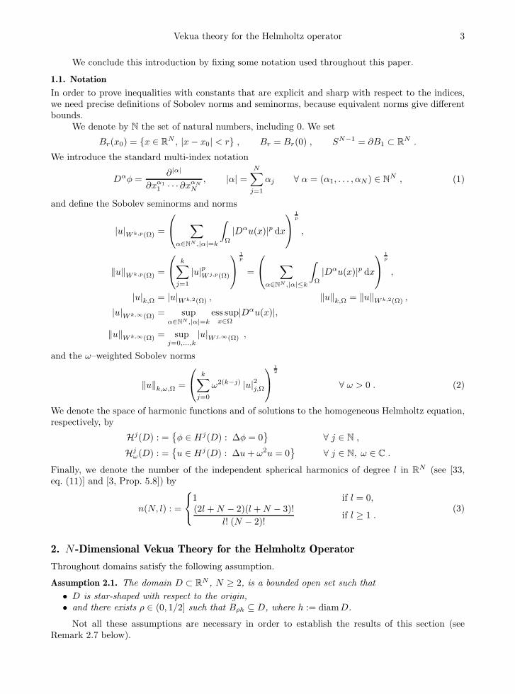
Theorem 2.5. Let D be a domain as in Assumption 2.1; the Vekua operators satisfy:

(i) V2 is the inverse of V1:

V1[

V2[φ]]

= V2[

V1[φ]]

= φ ∀ φ ∈ C(D) . (6)

(ii) If φ is harmonic in D, i.e.,

∆φ = 0 in D , (7)

then

∆V1[φ] + ω2V1[φ] = 0 in D .

(iii) If u is a solution of the homogeneous Helmholtz equation with wavenumber ω > 0 in D, i.e.,

∆u+ ω2u = 0 in D , (8)

then

∆V2[u] = 0 in D .

Theorem 2.5 states that the operators V1 and V2 are inverse to each other and map harmonicfunctions to solutions of the homogeneous Helmholtz equation and vice versa.

The results of this theorem were stated in [36, Chapter 1, § 13.2-3]. In two space dimensions, theoperator V1 followed from the general Vekua theory for elliptic PDEs; this implies that V1 is a bijectionbetween the space of complex harmonic function and the space of solutions of the homogeneousHelmholtz equation 1. The fact that the inverse of V1 can be written as the operator V2 (part (i) ofTheorem 2.5) was stated in [35], and the proof was skipped as an “easy calculation”, after reducingthe problem to a one-dimensional Volterra integral equation. Here, we give a completely self-containedand general proof of Theorem 2.5 merely using elementary calculus.

As in Theorem 2.5, in the following we will usually denote the solutions of the homogeneousHelmholtz equation with the letter u, and harmonic functions, as well as generic functions defined onD, with the letter φ.

Remark 2.6. Theorem 2.5 holds with the same proof also for every ω ∈ C, i.e., for the Helmholtzequation in lossy materials.

Remark 2.7. Theorem 2.5 holds also for an unbounded or irregular domain: the only necessary hypothe-ses are that D has to be open and star-shaped with respect to the origin. In fact the proof only relieson the local properties of the functions on the segment [0, x]. For the same reason, the singularities ofφ and u on the boundary of D do not affect the results of the theorem.

Theorem 2.5 can be proved by using elementary mathematical analysis results. We proceed byproving the parts (i) and (ii) separately.

Proof of Theorem 2.5, part (i). We define a function

g : [0,∞)× [0,∞) → R,

g(r, t) =ω√r t

2√r − t

J1(ω√r√r − t).

Note that if r < t the argument of the Bessel function J1 is imaginary on the standard branch cutbut the function g is always real-valued.

Using the change of variable s = t|x|, for every φ ∈ C(D) and for every x ∈ D, we can compute

V1[φ](x) = φ(x) +

∫ |x|

0

M1

(

x,s

|x|)

φ(

sx

|x|) 1

|x| ds

= φ(x) −∫ |x|

0

ω|x|2

√

s

|x|N−2

√

|x|√

|x| − s

1

|x| J1(

ω√

|x|√

|x| − s)

φ(

sx

|x|)

ds

1The proof in higher space dimensions might be contained in the Georgian language article [34] that is hard to obtain.


= φ(x) −∫ |x|

0

sN−4

2

|x|N−2

2

g(|x|, s) φ(

sx

|x|)

ds,

V2[φ](x) = φ(x) +

∫ |x|

0

M2

(

x,s

|x|)

φ(

sx

|x|) 1

|x| ds

= φ(x) −∫ |x|

0

iω|x|2

√

s

|x|N−3

√

|x|√

|x| − s

1

|x| J1(

iω√s√

|x| − s)

φ(

sx

|x|)

ds

= φ(x) +

∫ |x|

0

sN−4

2

|x|N−2

2

g(s, |x|) φ(

sx

|x|)

ds

because s ≤ |x| and we have fixed the sign√

s− |x| = i√

|x| − s. Note that in the expressions for thetwo operators the arguments of the functions g are swapped. Now we apply the first operator afterthe second one, switch the order of the integration in the resulting double integral and get

V1[

V2[φ]]

(x) =

[

φ(x) +

∫ |x|

0

sN−4

2

|x|N−2

2

g(s, |x|) φ(

sx

|x|)

ds

]

−∫ |x|

0

sN−4

2

|x|N−2

2

g(|x|, s)[

φ(

sx

|x|)

+

∫ s

0

zN−4

2

sN−2

2

g(z, s)φ(

zx

|x|)

dz

]

ds

=φ(x) +

∫ |x|

0

sN−4

2

|x|N−2

2

(

g(s, |x|)− g(|x|, s))

φ(

sx

|x|)

ds

−∫ |x|

0

zN−4

2

|x|N−2

2

φ(

zx

|x|)

∫ |x|

z

1

sg(z, s) g(|x|, s) ds dz.

The exchange of the order of integration is possible because φ is continuous and in the domain of

integration |s−1z−1g(|x|, s)g(z, s)| ≤ ω4

16 s |x| eω|x| thanks to (63), so Fubini theorem can be applied.

Notice that V1[

V2[φ]]

= V2[

V1[φ]]

, so we only have to show that V2 is right inverse of V1. In

order to prove that V1[

V2[φ]]

= φ it is enough to show that

g(t, r)− g(r, t) =

∫ r

t

g(t, s) g(r, s)

sds ∀ r ≥ t ≥ 0, (9)

so that all the integrals in the previous expression vanish, and we are done. Using (60), we expand gin power series (recall that, for k ≥ 0 integer, Γ(k + 1) = k!):

g(r, t) =ω2 r t

4

∑

l≥0

(−1)l ω2l rl (r − t)l

22l l! (l + 1)!, (10)

from which we get

g(t, r)− g(r, t) =ω2 r t

4

∑

l≥0

(−1)l ω2l (r − t)l(

(−t)l − rl)

22l l! (l + 1)!. (11)

We compute the following integral using the change of variables z = s−tr−t and the expression of the

beta integral∫ 1

0 (1− z)pzq dz = B(p+ 1, q + 1) =p! q!

(p+ q + 1)!:

∫ r

t

s(r−s)j(t−s)k ds = (−1)k(r−t)j+k+1

∫ 1

0

(1−z)jzk(

zr + (1−z)t)

dz

= (−1)k(r−t)j+k+1 j! k!

(j + k + 2)!

(

r(k+1) + t(j+1))

.

(12)


Thus, expanding the product of g(t, s) g(r, s) in a double power series, integrating term by term andusing the previous identity give

∫ r

t

g(t, s) g(r, s)

sds

(10)=

ω2 r t

4

∑

j,k≥0

(−1)j+k ω2(j+k+1) rj tk

22(j+k+1) j! (j + 1)! k! (k + 1)!

∫ r

t

s2(r − s)j(t− s)k

sds

(12)=

ω2 r t

4

∑

j,k≥0

(−1)j ω2(j+k+1) rj tk (r − t)j+k+1

22(j+k+1) (j + 1)! (k + 1)! (j + k + 2)!

(

r(k + 1) + t(j + 1))

(l=j+k+1)=

ω2 r t

4

∑

l≥1

ω2l (r − t)l

22l (l + 1)!

1

l!

l−1∑

j=0

l!(−1)j rj tl−j−1

(j + 1)! (l − j)!

(

r(l−j) + t(j+1))

=ω2 r t

4

∑

l≥1

ω2l (r − t)l

22l (l + 1)! l!

l−1∑

j=0

[

−(

l

j + 1

)

(−r)j+1 tl−j−1 +

(

l

j

)

(−r)j tl−j]

=ω2 r t

4

∑

l≥1

ω2l (r − t)l

22l (l + 1)! l!

[

−(t− r)l + tl + (t− r)l − (−r)l]

(11)= g(t, r)− g(r, t),

thanks to the binomial theorem and (11), where the term corresponding to l = 0 is zero. This proves(9), and the proof is complete.

Proof of Theorem 2.5, part (ii). Let φ be a harmonic function, then φ ∈ C∞(D), thanks to the regu-larity theorem for harmonic functions (see, e.g., [17, Corollary 8.11]). We prove that (∆+ω2)V1[φ](x) =0. In order to do that, we establish some useful identities.

We set r := |x| and compute

∂

∂|x|M1(x, t) = ω√1− t

∂

∂(ωr√1− t)

[

−√tN−2

2(1− t)ωr

√1− t J1(ωr

√1− t)

]

(65)= −ω

2r√tN−2

2J0(ωr

√1− t),

∆M1(x, t) =N − 1

r

∂

∂|x|M1(x, t) +∂2

∂|x|2M1(x, t)

=− ω2√tN−2

2

(

N J0(ωr√1− t)− ωr

√1− t J1(ωr

√1− t)

)

,

(13)

where the Laplacian acts on the x variable.Since M1 depends on x only through r, we can compute

∆(

M1(x, t)φ(tx))

= ∆M1(x, t) φ(tx) + 2∇M1(x, t) · ∇φ(tx) +M1(x, t)∆φ(tx)

= ∆M1(x, t) φ(tx) + 2∂

∂|x|M1(x, t)x

r· t∇φ

∣

∣

∣

tx+ 0

= ∆M1(x, t) φ(tx) + 2t

r

∂

∂|x|M1(x, t)∂

∂tφ(tx),

because ∂∂tφ(tx) = x · ∇φ

∣

∣

∣

tx.

Finally, we define an auxiliary function f1 : [0, h]× [0, 1] → R by

f1(r, t) =√tNJ0(ωr

√1− t).


This function verifies

∂

∂tf1(r, t) =

N√tN−2

2J0(ωr

√1− t) +

√tNωr

2√1− t

J1(ωr√1− t),

f1(r, 0) = 0, f1(r, 1) = 1.

At this point, we can use all these identities to prove that V1[φ] is a solution of the homogeneousHelmholtz equation:

(∆ + ω2)V1[φ](x) = ∆φ(x) + ω2φ(x) +

∫ 1

0

∆(

M1(x, t)φ(tx))

dt+

∫ 1

0

ω2M1(x, t)φ(tx) dt

= ω2φ(x) − ω2

∫ 1

0

√tNJ0(ωr

√1− t)

∂

∂tφ(tx) dt

− ω2

∫ 1

0

(

N√tN−2

2J0(ωr

√1− t)− ωr

√tN−2

2

1− t√1− t

J1(ωr√1− t)

+ωr

√tN−2

2√1− t

J1(ωr√1− t)

)

φ(tx) dt

= ω2φ(x) − ω2

∫ 1

0

(

f1(r, t)∂

∂tφ(tx) +

∂

∂tf1(r, t)φ(tx)

)

dt

= ω2

(

φ(x) −[

f1(r, t)φ(tx)]t=1

t=0

)

= 0.

We have used the values assumed by φ only in the segment [0, x] that lies inside D, because D is star-shaped with respect to 0. Thus, the values of the function φ and of its derivative are well defined andthe fundamental theorem of calculus applies, thanks to the regularity theorem for harmonic functions.

Now, let u be a solution of the homogeneous Helmholtz equation. Since interior regularity resultsalso hold for solutions of the homogeneous Helmholtz equation, we infer u ∈ C∞(D). In order to provethat ∆V2[u] = 0, we proceed as before and compute

∂

∂|x|M2(x, t) =ω2r

√tN−2

2J0(iωr

√

t(1 − t)),

∆M2(x, t) =ω2

√tN−2

2

(

N J0(iωr√

t(1 − t))− iωr√

t(1− t) J1(iωr√

t(1− t)))

,

∆(M2(x, t)u(tx)) = ∆M2(x, t)u(tx) + 2t

r

∂

∂rM2(x, t)

∂

∂tu(tx)− ω2t2M2(x, t)u(tx),

and we define the function

f2(r, t) =√tNJ0(iωr

√

t(1− t)),

which verifies

∂

∂tf2(r, t) =

N√tN−2

2J0(iωr

√

t(1− t))−√tNiωr(1− 2t)

2√

t(1− t)J1(iωr

√

t(1− t)),

f2(r, 0) = 0, f2(r, 1) = 1.

We conclude by computing the Laplacian of V2[u]:

∆V2[u](x) = ∆u(x) +

∫ 1

0

∆(

M2(x, t)u(tx))

dt

= −ω2u(x) + ω2

∫ 1

0

√tNJ0(iωr

√

t(1− t))∂

∂tu(tx) dt


+ ω2

∫ 1

0

√tN−2

2

(

N J0(iωr√

t(1− t))

−iωr√t1− t√1− t

J1(iωr√

t(1 − t)) +iωrt

√t√

1− tJ1(iωr

√

t(1 − t))

)

u(tx) dt

= −ω2u(x) + ω2

∫ 1

0

(

f2(r, t)∂

∂tu(tx) +

∂

∂tf2(r, t)u(tx)

)

dt = 0.

Remark 2.8. With a slight modification in the proof, it is possible to show that V1 transforms thesolutions of the homogeneous Helmholtz equation

∆φ+ ω20φ = 0

into solutions of

∆φ+ (ω20 + ω2)φ = 0

for every ω and ω0 ∈ C, and V2 does the converse.

3. Continuity of the Vekua Operators

In the following theorem, we establish the continuity of V1 and V2 in Sobolev norms with continuityconstants as explicit as possible.

Theorem 3.1. Let D be a domain as in the Assumption 2.1; the Vekua operators

V1 : Hj(D) → Hjω(D) , V2 : Hj

ω(D) → Hj(D) ,

with Hj(D) and Hjω(D) both endowed with the norm ‖·‖j,ω,D defined in (2), are continuous. More

precisely, for all space dimensions N ≥ 2, for all φ and u in Hj(D), j ≥ 0, solutions to (7) and (8),respectively, the following continuity estimates hold:

‖V1[φ]‖j,ω,D ≤ C1(N) ρ1−N

2 (1 + j)32N+ 1

2 ej(

1 + (ωh)2)

‖φ‖j,ω,D , (14)

‖V2[u]‖j,ω,D ≤ C2(N,ωh, ρ) (1 + j)32N− 1

2 ej ‖u‖j,ω,D , (15)

where the constant C1 > 0 depends only on the space dimension N , and C2 > 0 also depends on theproduct ωh and the shape parameter ρ. Moreover, we can establish the following continuity estimatesfor V2 with constants depending only on N :

‖V2[u]‖0,D ≤ CN ρ1−N

2

(

1 + (ωh)4)

e12(1−ρ)ωh

(

‖u‖0,D + h |u|1,D)

(16)

if N = 2, . . . , 5, u ∈ H1(D),

‖V2[u]‖j,ω,D ≤ CN ρ1−N

2 (1 + j)2N−1 ej(

1 + (ωh)4)

e34(1−ρ)ωh ‖u‖j,ω,D (17)

if N = 2, 3, j ≥ 1, u ∈ Hj(D),

and the following continuity estimates in L∞–norm:

‖V1[φ]‖L∞(D) ≤(

1 +

(

(1 − ρ)ωh)2

4

)

‖φ‖L∞(D) (18)

‖V2[u]‖L∞(D) ≤(

1 +

(

(1 − ρ)ωh)2

4e

12(1−ρ)ωh

)

‖u‖L∞(D) (19)

if N ≥ 2, φ, u ∈ L∞(D).


Theorem 3.1 states that the operators V1 and V2 preserve the Sobolev regularity when appliedto harmonic functions and solutions of the homogeneous Helmholtz equation (see Theorem 2.5). Forsuch functions, these operators are continuous from Hj(D) to itself with continuity constants thatdepend on the wavenumber ω only through the product ωh. In two and three space dimensions, wecan make explicit the dependence of the bounds on ωh. The only exception is the L2-continuity of V2(see (16)), where a weighted H1-norm appears on the right-hand side; this is due to the poor explicitinterior estimates available for the solutions of the homogeneous Helmholtz equation.

All the continuity constants are explicit with respect to the order of the Sobolev norm and dependon D only through its shape parameter ρ and its diameter h, the latter only appearing within theproduct ωh.

In the literature, there exist many proofs of the continuity of V1 and V2 in L∞-norm (in twospace dimensions); see, for example, [7, 15]. To our knowledge, the only continuity result in Sobolevnorms is the one given in [27, Section 4.2]: this holds for general PDEs and for norms with non-integerindices, but is restricted to the two-dimensional case, and the constants in the bounds are not explicitin the various parameters.

Since the proof of Theorem 3.1 is quite lengthy and requires several preliminary results, we givehere a short outline. In Lemma 3.2, a direct attempt to compute the Sobolev norms of Vξ[φ] showsthat two types of intermediate estimates are required. The first ones consist in bounds of the kernelfunctions M1 and M2 in W j,∞–norms; these are proved in Lemma 3.3. The second ones are interiorestimates for harmonic functions and for Helmholtz solutions: the former are well-known and recalledin Lemma 3.8, while the latter are proved in Lemma 3.11. Since we want explicit dependence of thebounding constants on the wave number, this step turns out to be the hardest one. Finally, we combineall these ingredients and prove Theorem 3.1.

From here on, if β is a multi-index in NN , we will denote by Dβ the corresponding differentialoperator with respect to the space variable x ∈ RN ; see (1).

Lemma 3.2. For ξ = 1, 2, j ≥ 0 and φ ∈ Hj(D), we have

|Vξ[φ]|2j,D ≤ 2 |φ|2j,D + 2(j + 1)3N−2e2jj∑

k=0

supt∈[0,1]

|Mξ(·, t)|2W j−k,∞(D) ·

∑

|β|=k

∫ 1

0

∫

D

∣

∣Dβφ(tx)∣

∣

2dxdt. (20)

Proof. From Definition 2.4, we have

∣

∣Vξ[φ]∣

∣

2

j,D≤ 2 |φ|2j,D + 2

∑

|α|=j

∫

D

∣

∣

∣

∣

∫ 1

0

Dα (Mξ(x, t)φ(tx)) dt

∣

∣

∣

∣

2

dx

≤ 2 |φ|2j,D + 2∑

|α|=j

∫

D

∫ 1

0

∣

∣

∣

∣

∣

∣

∑

β≤α

(

α

β

)

Dα−βMξ(x, t)Dβφ(tx)

∣

∣

∣

∣

∣

∣

2

dt dx

≤ 2 |φ|2j,D + 2

∫

D

∫ 1

0

∣

∣

∣

∣

∣

j∑

k=0

∑

|β|=k

∣

∣Dβφ(tx)∣

∣

∑

|α|=jα≥β

(

α

β

)

∣

∣Dα−βMξ(x, t)∣

∣

∣

∣

∣

∣

∣

2

dt dx,

where in the second inequality we have applied the Jensen inequality and the product (Leibniz) rule

for multi-indices (see [1, Sec. 1.1]); here, the binomial coefficient for multi-indices is(

αβ

)

=∏Ni=1

(

αi

βi

)

.

We multiply by the number(

N+k−1N−1

)

of the multi-indices β of length k in NN , in order to move thesquare inside the sum, and we obtain

∣

∣Vξ[φ]∣

∣

2

j,D≤ 2 |φ|2j,D + 2

∫

D

∫ 1

0

(j + 1)

j∑

k=0

(

N+k−1N−1

)


·∑

|β|=k

∣

∣Dβφ(tx)∣

∣

2

∣

∣

∣

∣

∣

∑

|α|=jα≥β

(

α

β

)

∣

∣Dα−βMξ(x, t)∣

∣

∣

∣

∣

∣

∣

2

dt dx

≤ 2 |φ|2j,D + 2(j + 1)(

N+j−1N−1

)

j∑

k=0

∑

|β|=k

∫

D

∫ 1

0

∣

∣Dβφ(tx)∣

∣

2dt dx

· supt∈[0,1]

|Mξ(·, t)|2W j−k,∞(D) sup|β|=k

[

∑

|α|=jα≥β

(

α

β

)

]2

;

the last factor can be bounded as

sup|β|=k

∑

|α|=jα≥β

N∏

i=1

(

αiβi

)

≤ sup|β|=k

∑

|α|=jα≥β

N∏

i=1

αβi

i

βi!≤∑

|α|=je

PNi=1

αi

≤ ej · #α ∈ NN , |α| = j = ej

(

N+k−1N−1

)

.

Finally, we note that, for every j ∈ N, N ≥ 2, we have(

N + j − 1

N − 1

)

=N + j − 1

N − 1

N + j − 2

N − 2· · · 1 + j

1≤ (1 + j)N−1 , (21)

from which the assertion follows.

Now we need to bound the terms present in (20). The next lemma provides W j,∞(D)–estimatesfor M1 and M2 uniformly in t. The proof relies on some properties of Bessel functions.

Lemma 3.3. The functions M1 and M2 satisfy the following bounds:

‖M1‖L∞(D×[0,1]) ≤(

(1− ρ) ω h)2

4, (22)

supt∈[0,1]

|M1(·, t)|W 1,∞(D) ≤(1− ρ) ω2 h

2, (23)

supt∈[0,1]

|M1(·, t)|W j,∞(D) ≤ωj

2(j + (1− ρ) ω h) ∀j ≥ 2, (24)

‖M2‖L∞(D×[0,1]) ≤(

(1− ρ) ω h)2

4e

12(1−ρ)ωh , (25)

supt∈[0,1]

|M2(·, t)|W 1,∞(D) ≤(1− ρ) ω2 h

2e

12(1−ρ)ωh, (26)

supt∈[0,1]

|M2(·, t)|W j,∞(D) ≤ωj

2j−1

(

j +(1− ρ) ω h

2

)

e34(1−ρ)ωh ∀j ≥ 2. (27)

Proof. Thanks to Remark 2.2, we have that supx∈D |x| ≤ (1 − ρ) h. Now, the L∞–inequalities (22)and (25) follow directly from (63).

Since M1 and M2 depend on x only through |x|, we obtain the W 1,∞ bounds (23) and (26):

supt∈[0,1]

|M1(·, t)|W 1,∞(D) = supt∈[0,1], x∈D

∣

∣

∣

∣

∂

∂|x|M1(x, t)

∣

∣

∣

∣

(65)

≤ supt∈[0,1],

|x|∈[0,(1−ρ)h]

∣

∣

∣

∣

∣

ω2|x|√tN−2

2J0(ω|x|

√1− t)

∣

∣

∣

∣

∣

(62)

≤ (1− ρ) ω2 h

2,


supt∈[0,1]

|M2(·, t)|W 1,∞(D)

(65)

≤ supt∈[0,1],

|x|∈[0,(1−ρ)h]

∣

∣

∣

∣

∣

ω2|x|√tN−2

2J0(iω|x|

√

t(1− t))

∣

∣

∣

∣

∣

(63)

≤ (1− ρ) ω2 h

2e

12(1−ρ)ωh.

In order to prove (24) and (27), we define the auxiliary complex-valued function f(s) = s J1(s).It is easy to verify by induction that its derivative of order k is

∂k

∂skf(s) = k

∂k−1

∂sk−1J1(s) + s

∂k

∂skJ1(s).

We can bound this derivative using (66) and the binomial theorem:∣

∣

∣

∣

∂k

∂skf(s)

∣

∣

∣

∣

=∣

∣

∣k1

2k−1

k−1∑

m=0

(−1)m(

k − 1

m

)

J2m−k+2(s) + s1

2k

k∑

m=0

(−1)m(

k

m

)

J2m−k+1(s)∣

∣

∣ (28)

≤ (k + |s|) maxl=1−k,...,1+k

|Jl(s)| .

The functions M1 and M2 are related to f by

M1(x, t) = −√tN−2

2(1− t)f(ω|x|

√1− t),

M2(x, t) = −√tN−4

2(1− t)f(iω|x|

√

t(1− t)),

so we can bound their derivatives of order j ≥ 2:

supt∈[0,1]

|M1|W j,∞(D) ≤ supt∈[0,1], x∈D

∣

∣

∣

∣

∂j

∂|x|jM1(x, t)

∣

∣

∣

∣

≤ supt∈[0,1], x∈D

∣

∣

∣

∣

∣

√tN−2

2(1− t)

(

ω√1− t

)j ∂j

∂(ω|x|√1− t)j

f(ω|x|√1− t)

∣

∣

∣

∣

∣

(28), (62)

≤ ωj

2(j + (1 − ρ)ωh),

supt∈[0,1]

|M2|W j,∞(D) ≤ supt∈[0,1], x∈D

∣

∣

∣

∣

∣

√tN−4

2(1− t)

(

iω√

t(1− t))j ∂j

∂(iω|x|√

t(1 − t))jf(iω|x|

√

t(1− t))

∣

∣

∣

∣

∣

(28), (63)

≤ ωj

2j−1

(

j +(1− ρ)ωh

2

)

e34(1−ρ)ωh.

Remark 3.4. With less detail the bounds of Lemma 3.3 for every j ≥ 0 can be summarized as:

supt∈[0,1]

|M1(·, t)|W j,∞(D) ≤ ωj(

j + (ωh)2)

, (29)

supt∈[0,1]

|M2(·, t)|W j,∞(D) ≤ ωj (1 + ωh) e34(1−ρ)ωh. (30)

We ignore the algebraic dependence on ρ because it will be absorbed in a generic bounding constant.In a shape regular domain, a precise lower bound for ρ ∈ (0, 12 ] can be used to reduce the exponentialdependence on ωh.

Remark 3.5. By performing some small changes in the proof of Lemma 3.3, we can extend Theorem 3.1to every ω ∈ C, similarly to Theorem 2.5 (see Remark 2.6). In fact, the case ω = 0 is trivial, sinceV1 and V2 reduce to the identity, while in general, Theorem 3.1 holds by substituting ω with |ω| in theestimates and in the definition of the weighted norm (2), and multiplying the right-hand side of (14)

by e32|ω|h (see Remark 1.2.5 in [21]).


Lemma 3.6. Let φ ∈ Hk(D), β ∈ NN be a multi-index of length |β| = k and Dβ be the correspondingdifferential operator in the variable x. Then

∫ 1

0

∫

D

∣

∣Dβφ(tx)∣

∣

2dxdt ≤

1

2k −N + 1

∥

∥Dβφ∥

∥

2

0,Dif 2k −N ≥ 0,

K∥

∥Dβφ∥

∥

2

0,D+(ρ

2

)2k+1 |D|2k + 1

∥

∥Dβφ∥

∥

2

L∞(B ρh2

)if 2k −N < 0,

where K = log 2ρ if 2k−N = −1, K =

(

2ρ

)N−1

if 2k−N < −1, |D| denotes the measure of D and ρ

is given in Assumption 2.1.

Proof. In the first case, we can simply compute the integral with respect to t with the change ofvariables y = tx:

∫ 1

0

∫

D

∣

∣Dβφ(tx)∣

∣

2dxdt =

∫ 1

0

∫

tD

t2|β|∣

∣Dβφ(y)∣

∣

2 dy

tNdt

≤ 1

2k −N + 1

∥

∥Dβφ∥

∥

2

0,D;

the set tD is included in D because D is star-shaped with respect to 0.In the case 2k − N < 0, the integral in t is not bounded so we need to split it in two parts,

treating the second part as before:∫ 1

0

∫

D

∣

∣Dβφ(tx)∣

∣

2dxdt =

∫ρ2

0

∫

D

∣

∣Dβφ(tx)∣

∣

2dxdt+

∫ 1

ρ2

∫

D

∣

∣Dβφ(tx)∣

∣

2dxdt

≤∫

ρ2

0

t2|β| dt|D|∥

∥Dβφ∥

∥

2

L∞(B ρh2

)+

∫ 1

ρ2

t2k−N∥

∥Dβφ∥

∥

2

0,tDdt

=1

2k + 1

(ρ

2

)2k+1

|D|∥

∥Dβφ∥

∥

2

L∞(B ρh2

)+

∫ 1

ρ2

t2k−N∥

∥Dβφ∥

∥

2

0,tDdt,

and the assertion comes from the expression

1∫

ρ2

t2k−N dt =

log2

ρif 2k −N = −1,

1−(

ρ2

)2k−N+1

2k −N + 1≤(

2

ρ

)N−1

if 2k −N < −1.

Remark 3.7. We can improve the bounds of Lemma 3.6 for every value of the multi-index length kwith the estimate

∫ 1

0

∫

D

∣

∣Dβφ(tx)∣

∣

2dxdt ≤

(

2

ρ

)N−1∥

∥Dβφ∥

∥

2

0,D+(ρ

2

)2k+1 |D|2k + 1

∥

∥Dβφ∥

∥

2

L∞(B ρh2

). (31)

From Lemma 3.6, it is clear that, in order to prove the continuity of V1 and V2 in the L2-normand in high-order Sobolev norms, we need interior estimates that bound the L∞-norm of φ and itsderivatives in a small ball contained in D with its L2-norm and Hj-norms in D. It is easy to find suchestimates for harmonic functions, thanks to the mean value theorem (see, e.g., Theorem 2.1 of [17]).

Notice that it is not possible to avoid the use of interior estimates for the continuity in Hj(D)when j ≥ N

2 , as the assertion of Lemma 3.6 might suggest: in fact, Lemma 3.2 requires to estimate∫ 1

0

∫

D

∣

∣Dβφ(tx)∣

∣

2dxdt for all the multi-index lengths |β| = k ≤ j, so we inevitably confront the cases

2k −N = −1 and 2k −N < −1.

Lemma 3.8 (Interior estimates for harmonic functions). Let φ be a harmonic function in BR(x),R > 0, then

|φ(x)|2 ≤ 1

RN |B1|‖φ‖20,BR(x) , (32)


where |B1| = πN2

Γ(N2+1)

is the volume of the unit ball in RN . If φ ∈ Hk(D) and β ∈ N

N , |β| ≤ k, then

∥

∥Dβφ∥

∥

2

L∞(B ρh2

)≤ 1

|B1|

(

2

ρh

)N∥

∥Dβφ∥

∥

2

0,D, (33)

Proof. By the mean value property of harmonic functions (see Theorem 2.1 of [17]) and the Jenseninequality, we get the first estimate:

|φ(x)|2 =

∣

∣

∣

∣

∣

1

|BR(x)|

∫

BR(x)

φ(y) dy

∣

∣

∣

∣

∣

2

≤ 1

|BR|

∫

BR(x)

|φ(y)|2 dy =1

RN |B1|‖φ‖20,BR(x) .

The second bound follows by applying the first one to the derivatives of φ, which are harmonic in theball B ρh

2

(x) ⊂ Bρh ⊂ D.

Remark 3.9. The interior estimates for harmonic functions are related to Cauchy’s estimates fortheir derivatives. Theorem 2.10 in [17] states that, given two domains Ω1 ⊂ Ω2 ⊂ RN such thatd(Ω1, ∂Ω2) = d, if φ is harmonic in Ω2, then for every multi-index α it holds

‖Dαφ‖L∞(Ω1)≤(

N |α|d

)|α|‖φ‖L∞(Ω2)

. (34)

In order to find analogous estimates for the Sobolev norms, we can combine (34) and (32) usingthe intermediate domain x ∈ RN : d(x,Ω1) <

d2 and obtain

‖Dαφ‖0,Ω1≤ CN,α|Ω1|N/2 d−|α|−N/2 ‖φ‖20,Ω2

,

but the order of the power of d is not satisfactory. In order to improve it, we represent the derivativesof a harmonic function ψ in B1 ⊂ RN using the Poisson kernel P :

Dαψ(y) =

∫

SN−1

ψ(z) Dα1P (y, z) dσ(z) y ∈ B1, ∀ α ∈ N

N ,

where the derivatives of P are taken with respect to the first variable (see (1.22) in [3]). Rewriting thisformula in y = 0 and then translating in a point x, if ψ is harmonic in B1(x), we have

Dαψ(x) =

∫

SN−1

ψ(x+ z) Dα1P (0, z) dσ(z) ∀ α ∈ N

N .

Given two domains Ω1 ⊂ Ω2 such that d(Ω1, ∂Ω2) = 1, if φ is harmonic in Ω2, it holds

∥

∥

∥Dαφ∥

∥

∥

0,Ω1

=

∫

Ω1

|Dαφ(x)|2 dx =

∫

Ω1

∣

∣

∣

∣

∫

SN−1

φ(x+ z) Dα1P (0, z) dσ(z)

∣

∣

∣

∣

2

dx

y=x+z

≤ |SN−1|∫

SN−1

(∫

Ω2

|φ(y)|2 dy

)

|Dα1P (0, z)|2 dσ(z) ≤ CN,α

∥

∥

∥φ∥

∥

∥

0,Ω2

,

where we have used the Jensen inequality and the Fubini theorem. By summing over all the multi-indices of the same length and scaling the domains such that Ω1 ⊂ Ω2 ⊂ RN and d(Ω1, ∂Ω2) = d, wefinally obtain

|φ|j+k,Ω1≤ CN,j,k d

−k |φ|j,Ω2, j, k ∈ N. (35)

We can use the bicontinuity of the Vekua operator to prove an analogous result for the solutionsof the Helmholtz equations; see Lemma 3.2.1 of [21].

The main tool used to prove the interior estimates for harmonic functions is the mean valuetheorem. For the solutions of the homogeneous Helmholtz equation, we have an analogous mean valueformula [14, page 289] but it does not provide good estimates.


Another way to prove interior estimates for the solutions of the homogeneous Helmholtz equationis to use the Green formula for the Laplacian in a ball, but this gives estimates that either involve theH1-norm of u on the right-hand side of the bound or give bad order in the domain diameter R.

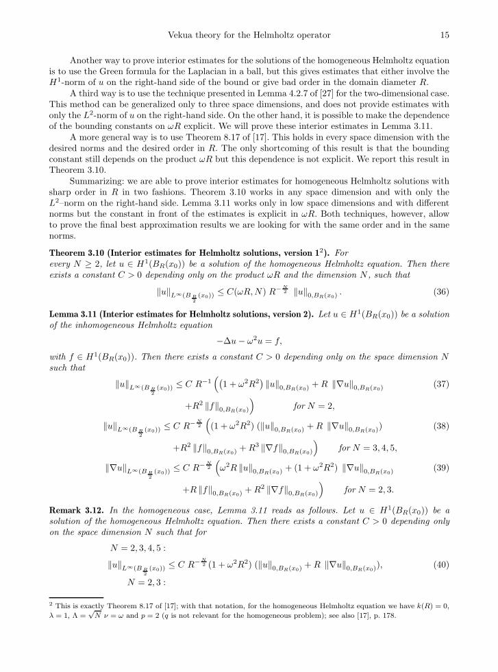
A third way is to use the technique presented in Lemma 4.2.7 of [27] for the two-dimensional case.This method can be generalized only to three space dimensions, and does not provide estimates withonly the L2-norm of u on the right-hand side. On the other hand, it is possible to make the dependenceof the bounding constants on ωR explicit. We will prove these interior estimates in Lemma 3.11.

A more general way is to use Theorem 8.17 of [17]. This holds in every space dimension with thedesired norms and the desired order in R. The only shortcoming of this result is that the boundingconstant still depends on the product ωR but this dependence is not explicit. We report this result inTheorem 3.10.

Summarizing: we are able to prove interior estimates for homogeneous Helmholtz solutions withsharp order in R in two fashions. Theorem 3.10 works in any space dimension and with only theL2–norm on the right-hand side. Lemma 3.11 works only in low space dimensions and with differentnorms but the constant in front of the estimates is explicit in ωR. Both techniques, however, allowto prove the final best approximation results we are looking for with the same order and in the samenorms.

Theorem 3.10 (Interior estimates for Helmholtz solutions, version 12). Forevery N ≥ 2, let u ∈ H1(BR(x0)) be a solution of the homogeneous Helmholtz equation. Then thereexists a constant C > 0 depending only on the product ωR and the dimension N , such that

‖u‖L∞(BR2

(x0))≤ C(ωR,N) R−N

2 ‖u‖0,BR(x0). (36)

Lemma 3.11 (Interior estimates for Helmholtz solutions, version 2). Let u ∈ H1(BR(x0)) be a solutionof the inhomogeneous Helmholtz equation

−∆u− ω2u = f,

with f ∈ H1(BR(x0)). Then there exists a constant C > 0 depending only on the space dimension Nsuch that

‖u‖L∞(BR2

(x0))≤ C R−1

(

(

1 + ω2R2)

‖u‖0,BR(x0)+R ‖∇u‖0,BR(x0)

+R2 ‖f‖0,BR(x0)

)

for N = 2,

(37)

‖u‖L∞(BR2

(x0))≤ C R−N

2

(

(1 + ω2R2) (‖u‖0,BR(x0)+R ‖∇u‖0,BR(x0)

)

+R2 ‖f‖0,BR(x0)+R3 ‖∇f‖0,BR(x0)

)

for N = 3, 4, 5,

(38)

‖∇u‖L∞(BR2

(x0))≤ C R−N

2

(

ω2R ‖u‖0,BR(x0)+ (1 + ω2R2) ‖∇u‖0,BR(x0)

+R ‖f‖0,BR(x0)+R2 ‖∇f‖0,BR(x0)

)

for N = 2, 3.

(39)

Remark 3.12. In the homogeneous case, Lemma 3.11 reads as follows. Let u ∈ H1(BR(x0)) be asolution of the homogeneous Helmholtz equation. Then there exists a constant C > 0 depending onlyon the space dimension N such that for

N = 2, 3, 4, 5 :

‖u‖L∞(BR2

(x0))≤ C R−N

2 (1 + ω2R2) (‖u‖0,BR(x0)+ R ‖∇u‖0,BR(x0)

), (40)

N = 2, 3 :

2 This is exactly Theorem 8.17 of [17]; with that notation, for the homogeneous Helmholtz equation we have k(R) = 0,

λ = 1, Λ =√

N ν = ω and p = 2 (q is not relevant for the homogeneous problem); see also [17], p. 178.


‖∇u‖L∞(BR2

(x0))≤ C R−N

2

(

ω2R ‖u‖0,BR(x0)+ (1 + ω2R2) ‖∇u‖0,BR(x0)

)

. (41)

Proof of Lemma 3.11. It is enough to bound |u(x0)| and |∇u(x0)|, because for all x ∈ BR2(x0) we can

repeat the proof using BR2(x) instead of BR(x0) with the same constants. We can also fix x0 = 0.

Let ϕ : R+ → [0, 1] be a smooth cut-off function such that

ϕ(r) =

1 |r| ≤ 14 ,

0 |r| ≥ 34 ,

and ϕR : RN → [0, 1], ϕR(x) := ϕ( |x|R

)

. Then

∇ϕR(x) = ϕ′( |x|R

)

x

R|x| , ∆ϕR(x) =1

R2ϕ′′( |x|R

)

+N − 1

R|x| ϕ′( |x|R

)

.

We define the average of u and two auxiliary functions on BR:

u :=1

|BR|

∫

BR

u(y) dy,

g(x) := u(x) ϕR(x), g(x) := (u(x)− u) ϕR(x);

their Laplacians are:

f(x) : = f1(x) + f2(x) + f3(x) := −∆g(x)

= −[

1

R2ϕ′′( |x|

R

)

+N − 1

R|x| ϕ′( |x|R

)

]

u(x)− 2ϕ′( |x|R

) x

R|x| · ∇u(x) + ϕ( |x|R

)

(ω2u(x) + f(x)),

f(x) : = f1(x) + f2(x) + f3(x) := −∆g(x)

= −[

1

R2ϕ′′( |x|

R

)

+N − 1

R|x| ϕ′( |x|R

)

]

(u(x)− u)− 2ϕ′( |x|R

) x

R|x| · ∇u(x) + ϕ( |x|R

)

(ω2u(x) + f(x)).

The fundamental solution formula for Poisson equation states that, if −∆a = b in RN , then

a(x) =

∫

RN

Φ(x− y) b(y) dy, with Φ(x) =

− 1

2πlog |x| N = 2,

|x|2−NN(N − 2)|B1|

N ≥ 3.(42)

The identity (42) holds for all b ∈ L2(BR), thanks to Theorem 9.9 of [17]. We notice that

|∇Φ(x)| =∣

∣

∣

∣

− 1

N |B1|x

|x|N∣

∣

∣

∣

=1

N |B1||x|1−N ∀ N ≥ 2.

We start by bounding |u(0)| for N = 2. In this case, it is easy to see that, for all R > 0, we have∫

BR

(

log |x| − logR)2

dx =π

2R2. (43)

We note that from the divergence theorem∫

BR

f(y) dy = −∫

BR

∆g(y) dy = −∫

∂BR

∇g(s) · n ds = 0,

because g ≡ 0 in R2 \B 34R and, since f = 0 outside B 3

4R then f has zero mean value in the whole R2.


We apply (42) with a = g and b = f ; using the Cauchy–Schwarz inequality, the identity (43) and

the fact that f has zero mean value in R2, we obtain:

|u(0)| = |g(0)| =∣

∣

∣

∣

− 1

2π

∫

R2

(

log |y| − logR)

f(y) dy

∣

∣

∣

∣

≤ 1

2π

√

π

2R ‖f‖0,B 3

4R

≤ CN,ϕR

(

1

R2‖u‖0,BR

+1

R‖∇u‖0,BR

+ ω2 ‖u‖0,BR+ ‖f‖0,BR

)

,

where the constant CN,ϕ depends only on N and ϕ; in the last step we have used the definition of f

and the fact that ϕ′( |x|R ) = 0 in BR4. The estimate (37) easily follows.

Proving all the other bounds (on |u(0)| for N ≥ 2 and on |∇u(0)| for N ≥ 2) is more involved.We fix p, p′ > 1 such that 1

p +1p′ = 1. For α > 0, we calculate

‖|y|α‖Lp′(BR) =

(

∫

SN−1

∫ R

0

rαp′

rN−1 dr dS

)1

p′

=

( |SN−1|αp′ +N

)

1

p′

Rα+N

p′ = CN,p′,αRα+N−N

p ,

(44)

that holds if αp′ +N 6= 0, that is equivalent to (α+N)p 6= N , for every N ≥ 2. We compute also

‖Φ‖Lp(B 34R\B 1

4R) = CN,p

(

|SN−1|∫ 3

4R

14R

r(2−N)p rN−1 dr

)1p

= CN,p |SN−1| 1p(

(

3

4R

)(2−N)p+N

−(

1

4R

)(2−N)p+N)

1p

= CN,p R2−N+N

p ,

(45)

for every p 6= NN−2 , N ≥ 3, and the analogue

‖∇Φ‖Lp(B 34R\B 1

4R) = CN,p

(

|SN−1|∫ 3

4R

14R

r(1−N)p rN−1 dr

)1p

= CN,p R1−N+N

p ,

(46)

that holds for every p 6= NN−1 , N ≥ 2.

Then, for all ψ ∈ H10 (BR), using scaling arguments, the continuity of the Sobolev embeddings

H10 (B1) → Lp(B1) which hold provided that 2 ≤ p ≤ 2N

N−2 , if N ≥ 3, and 2 ≤ p < ∞, if N = 2

(see [1, Th. 5.4,I,A-B]), and the Poincare inequality, we obtain

‖ψ‖Lp(BR) = RNp ‖ψ‖Lp(B1) ≤ CN,p R

Np ‖ψ‖1,B1

≤ CN,p RNp ‖∇ψ‖0,B1

≤ CN,p RNp+1−N

2 ‖∇ψ‖0,BR.

(47)

Now we can estimate u in the case N ≥ 3. From the Holder inequality for the pair of spacesLp

′

, Lp, p > 2 (thus, p′ < 2), and the fact that f1 ≡ f2 ≡ 0 in B 14R (see the definition of f), we can

write

|u(0)| = |g(0)| =∣

∣

∣

∣

∫

RN

Φ(x)f(x) dx

∣

∣

∣

∣

≤ ‖Φ‖Lp(B 34R\B 1

4R) ‖f1 + f2‖Lp′(B 3

4R\B 1

4R) + ‖Φ‖Lp′(BR) ‖f3‖Lp(BR).


Using (45) to bound the Lp-norm of Φ, the continuity of the embedding of Lp′

(B 34R \ B 1

4R) into

L2(B 34R \ B 1

4R) (recall that 1 < p′ < 2) with constant |B 3

4R \B 1

4R|

1

p′− 1

2 for the norm of f1 + f2, the

definition (42) of Φ and (44) with α = 2−N , which requires p > N2 , to bound the Lp

′

-norm of Φ, and

finally (47)which requires 2 ≤ p ≤ 2NN−2 , to bound the norm of f3 (recall that f3 ∈ H1

0 (BR)), we have

|u(0)| ≤ CN,pR2−N+N

p |B 34R|

1

p′− 1

2

∥

∥

∥f1 + f2

∥

∥

∥

0,B 34R\B 1

4R

+ CN,pR2−N

p RNp+1−N

2

∥

∥

∥∇f3∥

∥

∥

0,BR

Finally, using the definitions of the fi’s, |∇ϕR| ≤ 1RCϕ and 1

p + 1p′ = 1 we obtain

|u(0)| ≤CN,p,ϕR2−N+Np R

Np′

−N2

(

1

R2‖u‖0,BR

+1

R‖∇u‖0,BR

)

+ CN,p,ϕR3−N

2

(

ω2 ‖∇u‖0,BR+ ‖∇f‖0,BR

+1

Rω2 ‖u‖0,BR

+1

R‖f‖0,BR

)

≤CN,p,ϕ R−N2

(

(1 + ω2R2) ‖u‖0,BR+R (1 + ω2R2) ‖∇u‖0,BR

+R2 ‖f‖0,BR+R3 ‖∇f‖0,BR

)

.

The previous argument for bounding |u(0)| requires that there exists p such that N2 < p ≤ 2N

N−2 ,which is possible only if N < 6; this is the reason of the upper bound on the space dimension in thestatement.

In order to conclude this proof, we have to estimate |∇u(0)|. We use the same technique as

before, after differentiating the relation (42) with a = g and b = f . For every N ≥ 2, thanks to (46),

the embedding of Lp′

(B 34R \ B 1

4R) into L

2(B 34R \ B 1

4R), (44) with α = 1 −N and (47), that require

N < p ≤ 2NN−2 , we have

|∇u(0)| = |∇g(0)| =∣

∣

∣

∣

∫

RN

∇Φ(x)f (x) dx

∣

∣

∣

∣

≤ ‖∇Φ‖Lp(B 34R\B 1

4R) ‖f1 + f2‖Lp′(B 3

4R\B 1

4R) + ‖∇Φ‖Lp′(BR) ‖f3‖Lp(BR)

≤ CN,pR1−N+N

p |B 34R|

1

p′− 1

2 ‖f1 + f2‖0,B 34R\B 1

4R+ CN,pR

1−Np R

Np+1−N

2 ‖∇f3‖0,BR.

By using the Poincare-Wirtinger inequality, whose constant scales with R, to bound ‖u− u‖0,BR, we

obtain

|∇u(0)| ≤ CN,p,ϕ R−1−N

2

(

R−2 ‖u− u‖0,BR+R−1 ‖∇u‖0,BR

)

+ CN,p,ϕ R2−N

2

(

R−1∥

∥ω2u+ f∥

∥

0,BR+∥

∥∇(ω2u+ f)∥

∥

0,BR

)

≤ CN,p,ϕ R−N

2

(

ω2R ‖u‖0,BR+ (1 + ω2R2) ‖∇u‖0,BR

+R ‖f‖0,BR+R2 ‖∇f‖0,BR

)

,

The requirement that there exists p such that N < p ≤ 2NN−2 can be satisfied only if N < 4.

Lemma 3.11 is the only result in this section which we are not able to generalize to all the spacedimensions N ≥ 2. This is because in its proof we make use of a pair of conjugate exponents p andp′ such that the fundamental solution Φ of the Laplace equation (together with its gradient) belongs

to Lp′

(BR) and, at the same time, H1(BR) is continuously embedded in Lp(BR). This requirementyields the upper bounds on the space dimension we have required in the statement of Lemma 3.11.

Combining the results of the previous lemmas, we can now prove Theorem 3.1.


Proof of Theorem 3.1. We start by proving the continuity bound (14) for V1. For every j ∈ N, N ≥ 2,φ ∈ Hj(D), inserting (29) and (31) into (20) with ξ = 1, we have

|V1[φ]|j,D ≤[

2 |φ|2j,D + 2(1 + j)3N−2e2jj∑

k=0

ω2(j−k)(j − k + (ωh)2)2

·(

(

2

ρ

)N−1

|φ|2k,D +(ρ

2

)2k+1 |D|2k + 1

∑

|β|=k

∥

∥Dβφ∥

∥

2

L∞(B ρh2

)

)]12

.

Then, using the interior estimates (33), we get

|V1[φ]|j,D ≤ CN (1 + j)32N−1+1 ej

(

1 + (ωh)2)

[

j∑

k=0

ω2(j−k)(

ρ1−N + ρ2k+1 |D|(ρh)N

)

|φ|2k,D

]12

≤ CN ρ1−N

2 (1 + j)32N ej

(

1 + (ωh)2)

‖φ‖j,ω,D ,

by the definition of weighted Sobolev norms (2), and because |D| ≤ hN and ρ < 1. The constant CNdepends only on the dimension N of the space. Passing from the seminorms to the complete Sobolevnorms gives an extra coefficient (1 + j)1/2 and the bound (14) follows.

In order to prove the continuity bound (15) for V2, we proceed similarly. For every j ∈ N, N ≥ 2,u ∈ Hj

ω(D), inserting (30) and (31) into (20) with ξ = 2, we have

|V2[u]|j,D ≤[

2 |u|2j,D + 2(1 + j)3N−2e2jj∑

k=0

ω2(j−k)(1 + ωh)2e32(1−ρ)ωh

·(

(

2

ρ

)N−1

|u|2k,D +(ρ

2

)2k+1 |D|2k + 1

∑

|β|=k

∥

∥Dβu∥

∥

2

L∞(B ρh2

)

)]12

(36)

≤ C(N,ωh, ωρh) (1 + j)32N−1 ej

[

j∑

k=0

ω2(j−k)(

ρ1−N + ρ2k+1 |D|(ρh)N

)

|u|2k,D

]12

≤ C(N,ωh, ρ) (1 + j)32N−1 ej ‖u‖j,ω,D .

Again, passing from the seminorms to the complete Sobolev norms gives an extra coefficient (1+ j)1/2

and the bound (15) follows.

Now we proceed by proving the bounds (16), (17) and (19) for V2 with constants depending onlyon N .

For the continuity bound (16) for the V2 operator from H1(D) to L2(D), we repeat the samereasoning as above. If u ∈ H1

ω(D), N = 2, . . . , 5, using the definition of V2, (25), (31) and (40), wehave

‖V2[u]‖0,D ≤[

2 ‖u‖20,D + 2 ‖M2‖2L∞(D×[0,1])

∫ 1

0

∫

D

|u(tx)|2 dxdt

]12

≤[

2 ‖u‖20,D + 2

(

(ωh)2

4e

12(1−ρ)ωh

)2 [(2

ρ

)N−1

‖u‖20,D

+ρ

2|D|(

CN (ρh)−N2

(

1 + (ωρh)2)(

‖u‖0,D + ρh ‖∇u‖0,D)

)2]]

12

≤CN ρ1−N

2

(

1 + (ωh)4)

e12(1−ρ)ωh( ‖u‖0,D + ρh ‖∇u‖0,D

)

,


which immediately gives (16).Let us now prove (17). To this end, given a multi-index β ∈ NN , we need to bound

∥

∥Dβu∥

∥

L∞(B ρh2

).

If |β| = 0, for N = 2, 3, 4, 5, we simply use (40) and get∥

∥Dβu∥

∥

L∞(B ρh2

)= ‖u‖L∞(B ρh

2

) (48)

≤ CN (ρh)−N2 (1 + ω2ρ2h2)

(

‖u‖0,D + ρh ‖∇u‖0,D)

.

If |β| = j ≥ 1, we note that there exists another multi-index α ∈ NN of length |α| = j − 1, such thatfor N = 2, 3 and u ∈ Hj

ω(D) it holds∥

∥Dβu∥

∥

L∞(B ρh2

)≤ ‖∇Dαu‖L∞(B ρh

2

) (49)

≤ CN (ρh)−N2

(

ω2ρh ‖Dαu‖0,D +(

1 + (ωρh)2)

‖∇Dαu‖0,D)

,

thanks to (41). Notice that the restriction to N = 2, 3 in this proof is due to the use of (41). Again,inserting (30) and (31) into (20) with ξ = 2 gives

|V2[u]|j,D ≤ CN

[

|u|2j,D + (1 + j)3N−2 e2jj∑

k=0

ω2(j−k)(1 + ωh)2e32(1−ρ)ωh

·(

ρ1−N |u|2k,D + ρ2k+1|D|∑

|β|=k

∥

∥Dβu∥

∥

2

L∞(B ρh2

)

)

]12

≤ CN (1 + j)32N−1 ej (1 + ωh) e

34(1−ρ)ωh

·[

j∑

k=0

ω2(j−k)(

ρ1−N |u|2k,D + ρ2k+1|D|∑

|β|=k

∥

∥Dβu∥

∥

2

L∞(B ρh2

)

)

]12

,

and thus, as a consequence of (48) and (49), we obtain

|V2[u]|j,D ≤ CN (1 + j)32N−1 ej (1 + ωh) e

34(1−ρ)ωh

·[

ω2jρ1−N(

‖u‖20,D +|D|hN

(1 + ω2ρ2h2)2(

‖u‖0,D + ρh ‖∇u‖0,D)2)

+

j∑

k=1

ω2(j−k)ρ1−N(

|u|2k,D + ρ2k(

N+k−1N−1

) |D|hN

·(

ω2ρh |u|k−1,D + (1 + ω2ρ2h2) |u|k,D)2)

]12

≤ CN (1 + j)32N−1 ρ

1−N2 ej (1 + ωh) e

34(1−ρ)ωh

·[

ω2j(1 + ω2h2)2(

‖u‖0,D + h ‖∇u‖0,D)2

+

j∑

k=1

ω2(j−k)(1 + k)N−1(

ω2h |u|k−1,D + (1 + ω2h2) |u|k,D)2]

12

≤ CN (1 + j)2N− 32 ρ

1−N2 ej (1 + ωh) e

34(1−ρ)ωh

·[

(

1 + (ωh)2)2ω2j ‖u‖20,D +

(

(ωh)2 + (ωh)6)

ω2(j−1) |u|21,D


+ (ωh)2j∑

k=1

ω2(j−k+1) |u|2k−1,D +(

1 + (ωh)2)2

j∑

k=1

ω2(j−k) |u|2k,D

]12

≤ CN (1 + j)2N− 32 ρ

1−N2 ej

(

1 + (ωh)4)

e34(1−ρ)ωh ‖u‖j,ω,D ,

where the binomial coefficient comes from the number of the multi-indices |β| = k and is bounded by(21). As before, passing from the seminorms to the complete Sobolev norms gives an extra coefficient(1 + j)1/2 and the bound (17) follows.

Finally, we prove the continuity of V1 and V2 in the L∞-norm stated in (18), (19). Thanks to thedefinition of V1 and V2, the bounds (22) and (25), we have

‖V1[φ]‖L∞(D) ≤(

1 + ‖M1‖L∞(D×[0,1])

)

‖φ‖L∞(D)

≤(

1 +

(

(1− ρ)ωh)2

4

)

‖φ‖L∞(D) ,

‖V2[u]‖L∞(D) ≤(

1 +

(

(1− ρ)ωh)2

4e

12(1−ρ)ωh

)

‖u‖L∞(D) ,

that holds for every φ, u ∈ L∞(D) and for every N ≥ 2. This proves (18) and (19), the proof ofTheorem 3.1 is complete.

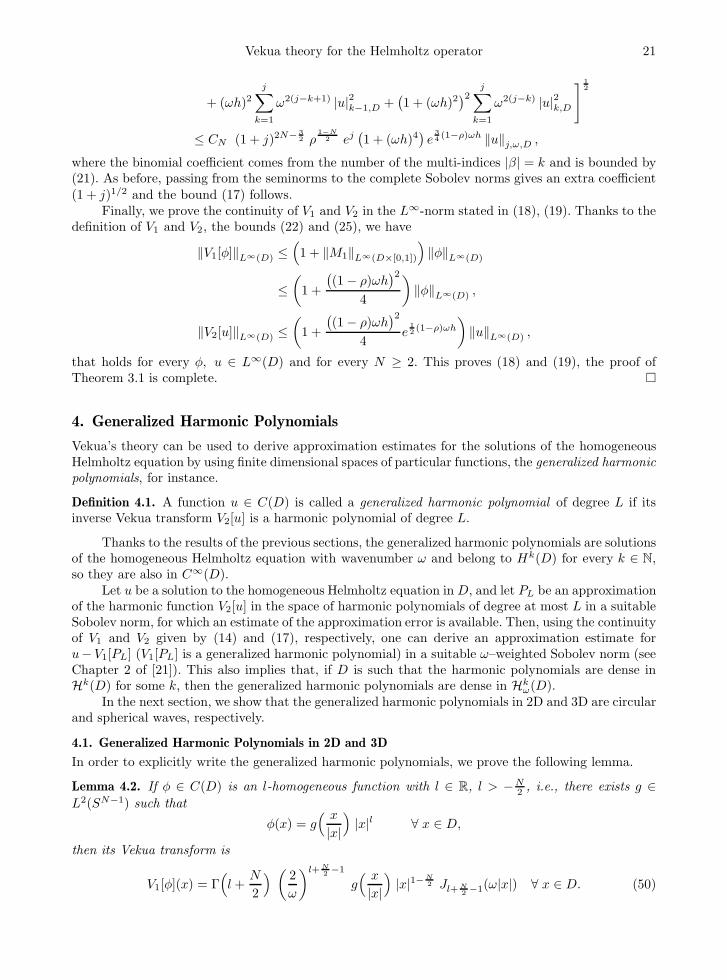
4. Generalized Harmonic Polynomials

Vekua’s theory can be used to derive approximation estimates for the solutions of the homogeneousHelmholtz equation by using finite dimensional spaces of particular functions, the generalized harmonicpolynomials, for instance.

Definition 4.1. A function u ∈ C(D) is called a generalized harmonic polynomial of degree L if itsinverse Vekua transform V2[u] is a harmonic polynomial of degree L.

Thanks to the results of the previous sections, the generalized harmonic polynomials are solutionsof the homogeneous Helmholtz equation with wavenumber ω and belong to Hk(D) for every k ∈ N,so they are also in C∞(D).

Let u be a solution to the homogeneous Helmholtz equation in D, and let PL be an approximationof the harmonic function V2[u] in the space of harmonic polynomials of degree at most L in a suitableSobolev norm, for which an estimate of the approximation error is available. Then, using the continuityof V1 and V2 given by (14) and (17), respectively, one can derive an approximation estimate foru−V1[PL] (V1[PL] is a generalized harmonic polynomial) in a suitable ω–weighted Sobolev norm (seeChapter 2 of [21]). This also implies that, if D is such that the harmonic polynomials are dense inHk(D) for some k, then the generalized harmonic polynomials are dense in Hk

ω(D).In the next section, we show that the generalized harmonic polynomials in 2D and 3D are circular

and spherical waves, respectively.

4.1. Generalized Harmonic Polynomials in 2D and 3D

In order to explicitly write the generalized harmonic polynomials, we prove the following lemma.

Lemma 4.2. If φ ∈ C(D) is an l-homogeneous function with l ∈ R, l > −N2 , i.e., there exists g ∈

L2(SN−1) such that

φ(x) = g( x

|x|)

|x|l ∀ x ∈ D,

then its Vekua transform is

V1[φ](x) = Γ(

l +N

2

)

(

2

ω

)l+N2−1

g( x

|x|)

|x|1−N2 Jl+N

2−1(ω|x|) ∀ x ∈ D. (50)


Proof. Using the Beta integral∫ 1

0 ta(1− t)b dt = Γ(a+1) Γ(b+1)

Γ(a+b+2) , a, b > −1, we can directly compute the

Vekua transform from the definition of V1:

V1[φ](x) = g( x

|x|)

|x|l +∫ 1

0

g( x

|x|)

(|x|t)l M1(x, t) dt

= g( x

|x|)

|x|l(

1 +

∫ 1

0

tlM1(x, t) dt

)

= g( x

|x|)

|x|l

1−

∫ 1

0

tl+N2−1∑

j≥0

(−1)j(

ω|x|2

)2j+2

(1 − t)j

j! (j + 1)!dt

= g( x

|x|)

|x|l

1−

∑

j≥0

(−1)j(

ω|x|2

)2j+2

j! (j + 1)!

Γ(

l+ N2

)

Γ(j + 1)

Γ(

l+ N2 + j + 1

)

k=j+1= g

( x

|x|)

|x|l

1 +

∑

k≥1

(−1)k(

ω|x|2

)2k

k! Γ(

l+ N2 + k

) Γ(

l+N

2

)

= g( x

|x|)

|x|l∑

k≥0

(−1)k(

ω|x|2

)2k

k! Γ(

l + N2 + k

) Γ(

l +N

2

)

= Γ(

l+N

2

)

g( x

|x|)

|x|1−N2

(

2

ω

)l+N2−1∑

k≥0

(−1)k(

ω|x|2

)2k+l+N2−1

k! Γ(

l+ N2 + k

)

= Γ(

l+N

2

)

(

2

ω

)l+N2−1

g( x

|x|)

|x|1−N2 Jl+N

2−1(ω|x|).

The condition l > −N2 is necessary to ensure a finite value of the integral

∫ 1

0 tl+N

2−1(1 − t)j dt.

As a consequence, the general (non homogeneous) harmonic polynomial of degree L and itsVekua transform can be written, in terms of spherical harmonics Yl,m (see [2,33]) and hypersphericalBessel functions jNl (see the Appendix), by

P (x) =L∑

l=0

n(N,l)∑

m=1

al,m |x|l Yl,m( x

|x|)

, (51)

V1[P ](x) = |x|1−N2

L∑

l=0

n(N,l)∑

m=1

al,m Γ(

l+N2

)

(

2

ω

)l+N2−1

Yl,m

( x

|x|)

Jl+N2−1(ω|x|)

=

2N2−1∑L

l=0

∑n(N,l)m=1 al,m Γ

(

l + N2

) (

2ω

)lYl,m

(

x|x|)

jNl (ω|x|), N even,

2N−1

2√π

∑Ll=0

∑n(N,l)m=1 al,m Γ

(

l + N2

) (

2ω

)lYl,m

(

x|x|)

jNl (ω|x|), N odd.(52)

If N = 2, identifying R2 = C and using the complex variable z = reiψ , using directly (50), we have

P (z) =

L∑

l=−Lal r

|l| eilψ , (53)

V1[P ](z) =

L∑

l=−Lal |l|!

(

2

ω

)|l|eilψ J|l|(ωr). (54)


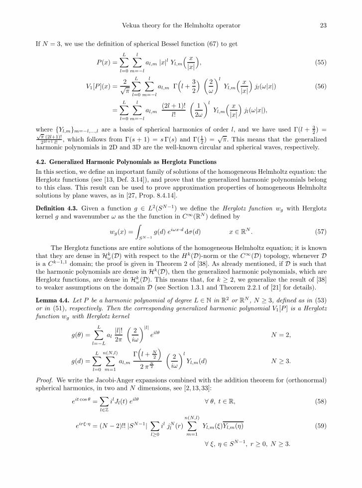
If N = 3, we use the definition of spherical Bessel function (67) to get

P (x) =

L∑

l=0

l∑

m=−lal,m |x|l Yl,m

( x

|x|)

, (55)

V1[P ](x) =2√π

L∑

l=0

l∑

m=−lal,m Γ

(

l +3

2

)

(

2

ω

)l

Yl,m

( x

|x|)

jl(ω|x|) (56)

=

L∑

l=0

l∑

m=−lal,m

(2l + 1)!

l!

(

1

2ω

)l

Yl,m

( x

|x|)

jl(ω|x|),

where Yl,mm=−l,...,l are a basis of spherical harmonics of order l, and we have used Γ(l + 32 ) =√

π (2l+1)!22l+1 l! , which follows from Γ(s + 1) = sΓ(s) and Γ(12 ) =

√π. This means that the generalized

harmonic polynomials in 2D and 3D are the well-known circular and spherical waves, respectively.

4.2. Generalized Harmonic Polynomials as Herglotz Functions

In this section, we define an important family of solutions of the homogeneous Helmholtz equation: theHerglotz functions (see [13, Def. 3.14]), and prove that the generalized harmonic polynomials belongto this class. This result can be used to prove approximation properties of homogeneous Helmholtzsolutions by plane waves, as in [27, Prop. 8.4.14].

Definition 4.3. Given a function g ∈ L2(SN−1) we define the Herglotz function wg with Herglotzkernel g and wavenumber ω as the the function in C∞(RN ) defined by

wg(x) =

∫

SN−1

g(d) eiωx·d dσ(d) x ∈ RN . (57)

The Herglotz functions are entire solutions of the homogeneous Helmholtz equation; it is knownthat they are dense in Hk

ω(D) with respect to the Hk(D)-norm or the C∞(D) topology, whenever Dis a Ck−1,1 domain; the proof is given in Theorem 2 of [38]. As already mentioned, if D is such thatthe harmonic polynomials are dense in Hk(D), then the generalized harmonic polynomials, which areHerglotz functions, are dense in Hk

ω(D). This means that, for k ≥ 2, we generalize the result of [38]to weaker assumptions on the domain D (see Section 1.3.1 and Theorem 2.2.1 of [21] for details).

Lemma 4.4. Let P be a harmonic polynomial of degree L ∈ N in R2 or RN , N ≥ 3, defined as in (53)or in (51), respectively. Then the corresponding generalized harmonic polynomial V1[P ] is a Herglotzfunction wg with Herglotz kernel

g(θ) =

L∑

l=−Lal

|l|!2π

(

2

iω

)|l|eilθ N = 2,

g(d) =

L∑

l=0

n(N,l)∑

m=1

al,mΓ(

l + N2

)

2 πN2

(

2

iω

)l

Yl,m(d) N ≥ 3.

Proof. We write the Jacobi-Anger expansions combined with the addition theorem for (orthonormal)spherical harmonics, in two and N dimensions, see [2, 13, 33]:

eit cos θ =∑

l∈Z

ilJl(t) eilθ ∀ θ, t ∈ R, (58)

eirξ·η = (N − 2)!! |SN−1|∑

l≥0

il jNl (r)

n(N,l)∑

m=1

Yl,m(ξ)Yl,m(η) (59)

∀ ξ, η ∈ SN−1, r ≥ 0, N ≥ 3.


These series converge absolutely and uniformly on compact subsets of RN . Now we only have to usethese formulas to verify that the Herglotz functions with the kernels written above correspond to (54)and (52), respectively.

In two space dimensions with the polar coordinates z = r eiψ we have

wg(z) =

∫ 2π

0

L∑

l=−Lal

|l|!2π

(

2

iω

)|l|eilθ eiωr(cosψ,sinψ)·(cos θ,sin θ) dθ

=

L∑

l=−Lal

|l|!2π

(

2

iω

)|l| ∫ 2π

0

eilθ eiωr cos(ψ−θ) dθ

(58)=

L∑

l=−Lal

|l|!2π

(

2

iω

)|l| ∫ 2π

0

eilθ∑

l′∈Z

il′

Jl′(ωr) eil′(ψ−θ) dθ

=

L∑

l=−L

∑

l′∈Z

al|l|!2π

(

2

iω

)|l|il

′

Jl′(ωr) eilψ

∫ 2π

0

ei(l−l′)θ dθ

(61)=

L∑

l=−Lal |l|!

(

2

ω

)|l|J|l|(ωr) e

ilψ (54)= V1[P ](z),

where in the second last step we have used the identity∫ 2π

0ei(l−l

′)θ dθ = 2π δl,l′ . In the previouschain of equalities, we could exchange the order of summation and integration because the serie in l′

converges uniformly and absolutely in [0, 2π], thanks to (63).

In higher space dimensions, we use the orthonormality of the spherical harmonics∫

SN−1 Yl,mYl′,m′

= δl,l′δm,m′ :

wg(x) =

∫

SN−1

L∑

l=0

n(N,l)∑

m=1

al,mΓ(

l+ N2

)

2πN2

(

2

iω

)l

Yl,m(d) eiωx·d dσ(d)

(59)=

∫

SN−1

L∑

l=0

n(N,l)∑

m=1

al,mΓ(

l+ N2

)

2πN2

(

2

iω

)l

Yl,m(d)

·∑

l′≥0

n(N,l′)∑

m′=1

(N − 2)!! |SN−1| il′ jNl′ (ω|x|) Yl′,m′

( x

|x|)

Yl′,m′(d) dσ(d)

=(N − 2)!!

Γ(

N2

)

L∑

l=0

n(N,l)∑

m=1

al,m Γ(

l +N

2

)

(

2

ω

)l

Yl,m

( x

|x|)

jNl (ω|x|)

(52), (68)= V1[P ](x),

where in the second last step we have used the formula |SN−1| = 2πN2 /Γ

(

N2

)

.

Lemma 4.4 also gives an easy formula to compute the Vekua transform of any Herglotz functionwg, given the expansion of its kernel g in harmonics.

Appendix A. Bessel Functions

We denote the usual Bessel functions of the first kind by Jν(z) and the spherical Bessel functions ofthe first kind by jν(z). The first ones are defined, for every ν, z ∈ C, as

Jν(z) =

∞∑

t=0

(−1)t

t! Γ(t+ ν + 1)

(z

2

)2t+ν

, (60)


where Γ is the gamma function. When ν /∈ Z and z belongs to the segment [−∞, 0], Jν(z) is notsingle-valued. When ν ∈ Z, Jν is an entire function.

We list some properties of these functions (references can be found in [26, 37]):

J−k(z) = (−1)kJk(z) ∀ k ∈ Z, (61)

Im(

Jk(t))

= 0, Re(

Jk(it))

= 0 ∀ k ∈ Z, t ∈ R,

|Jk(t)| ≤ 1 ∀ k ∈ Z, t ∈ R, (62)

|Jν(z)| ≤e| Im z|

Γ(ν + 1)

( |z|2

)ν

∀ ν > −1

2, z ∈ C, (63)

J0(0) = 1, Jk(0) = 0 ∀ k ∈ Z \ 0,∂

∂zJν(z) =

1

2(Jν−1(z)− Jν+1(z)) , (64)

∂

∂z

(

zkJk(z))

= zkJk−1(z),

∂

∂zJ0(z) = −J1(z),

∂

∂z(zJ1(z)) = zJ0(z), (65)

∂l

∂zlJk(z) =

1

2l

l∑

m=0

(−1)m(

l

m

)

J2m−l+k(z). (66)

The last equality can be easily proved by induction from (64).The spherical Bessel functions are defined as

jν(z) =

√

π

2zJν+ 1

2(z). (67)

These functions are a particular case of the so-called hyperspherical Bessel functions (see [2] p. 52):

jNk (z) =

∞∑

t=0

(−1)t z2t+k

(2t)!! (N + 2t+ 2k − 2)!!=

z1−N2 Jk+N

2−1(z), N even,

√

π2 z

1−N2 Jk+N

2−1(z), N odd,

Jk(z) = j2k(z), jk(z) = j3k(z).

The above equality is proved using (60) and

(2m)!! = 2mm!, (2m+ 1)!! =Γ(

m+ 32

)

2m+1

√π

, m ∈ N. (68)

References

[1] R. Adams, Sobolev spaces, Pure and Applied Mathematics, Academic Press, 1975.

[2] J. Avery, Hyperspherical Harmonics: applications in quantum theory, Reidel texts in the mathematicalsciences, Kluwer Academic Publishers, 1989.

[3] S. Axler, P. Bourdon, and W. Ramey, Harmonic function theory, Graduate Texts in Mathematics,Springer-Verlag, New York, 2001.

[4] I. Babuska and J. Melenk, The partition of unity method, Int. J. Numer. Methods Eng., 40 (1997),pp. 727–758.

[5] A. H. Barnett and T. Betcke, Stability and convergence of the method of fundamental solutions forHelmholtz problems on analytic domains, J. Comput. Phys., 227 (2008), pp. 7003–7026.

[6] , An exponentially convergent nonpolynomial finite element method for time-harmonic scatteringfrom polygons, SIAM J. Sci. Comput., 32 (2010), pp. 1417–1441.

[7] T. Betcke, Numerical computation of eigenfunctions of planar regions, PhD thesis, University of Oxford,2005.

[8] O. Cessenat and B. Despres, Application of an ultra weak variational formulation of elliptic PDEs tothe two-dimensional Helmholtz equation, SIAM J. Numer. Anal., 35 (1998), pp. 255–299.


[9] A. Charalambopoulos and G. Dassios, On the Vekua pair in spheroidal geometry and its role insolving boundary value problems, Appl. Anal., 81 (2002), pp. 85–113.

[10] D. Colton, Bergman operators for elliptic equations in three independent variables, Bull. Amer. Math.Soc., 77 (1971), pp. 752–756.

[11] , Integral operators for elliptic equations in three independent variables. I, Applicable Anal., 4(1974/75), pp. 77–95.

[12] , Integral operators for elliptic equations in three independent variables. II, Applicable Anal., 4(1974/75), pp. 283–295.

[13] D. Colton and R. Kress, Inverse Acoustic and Electromagnetic Scattering Theory, vol. 93 of AppliedMathematical Sciences, Springer, Heidelberg, 2nd ed., 1998.

[14] R. Courant and D. Hilbert, Methods of mathematical physics. Volume II: partial differential equations,Interscience Publishers, 1962.

[15] S. C. Eisenstat, On the rate of convergence of the Bergman-Vekua method for the numerical solution ofelliptic boundary value problems, SIAM J. Numer. Anal., 11 (1974), pp. 654–680.

[16] C. Farhat, I.Harari, and L. Franca, The discontinuous enrichment method, Comput. Methods Appl.Mech. Eng., 190 (2001), pp. 6455–6479.

[17] D. Gilbarg and N. Trudinger, Elliptic Partial Differential Equations of Second Order, Classics inMathematics, Springer-Verlag, 2nd ed., 1983.

[18] R. P. Gilbert and C. Y. Lo, On the approximation of solutions of elliptic partial differential equationsin two and three dimensions, SIAM J. Math. Anal., 2 (1971), pp. 17–30.

[19] C. Gittelson, R. Hiptmair, and I. Perugia, Plane wave discontinuous Galerkin methods: analysis ofthe h-version, M2AN Math. Model. Numer. Anal., 43 (2009), pp. 297–332.

[20] P. Henrici, A survey of I. N. Vekua’s theory of elliptic partial differential equations with analytic coeffi-cients, Z. Angew. Math. Phys., 8 (1957), pp. 169–202.

[21] R. Hiptmair, A. Moiola, and I. Perugia, Approximation by plane waves, Preprint 2009-27, SAMReport, ETH Zurich, Switzerland, 2009.

[22] , Plane wave discontinuous Galerkin methods for the 2D Helmholtz equation: analysis of the p-version, SIAM J. Numer. Anal., 49 (2011), pp. 264–284.

[23] N. T. Hop, Some extensions of I. N. Vekua’s method in higher dimensions. I. Integral representation ofsolutions of an elliptic system. Properties of solutions, Math. Nachr., 130 (1987), pp. 17–34.

[24] , Some extensions of I. N. Vekua’s method in higher dimensions. II. Boundary value problems, Math.Nachr., 130 (1987), pp. 35–46.

[25] M. Ikehata, Probe method and a Carleman function, Inverse Problems, 23 (2007), pp. 1871–1894.

[26] N. Lebedev, Special functions and their applications, Prentice-Hall, Englewood Cliffs, N.J., 1965.

[27] J. Melenk, On Generalized Finite Element Methods, PhD thesis, University of Maryland, 1995.

[28] , Operator adapted spectral element methods I: harmonic and generalized harmonic polynomials,Numer. Math., 84 (1999), pp. 35–69.

[29] J. Melenk and I. Babuska, Approximation with harmonic and generalized harmonic polinomials in thepartition of unit method, Comput. Assist. Mech. Eng. Sci., 4 (1997), pp. 607–632.

[30] A. Moiola, Approximation properties of plane wave spaces and application to the analysis of the planewave discontinuous Galerkin method, Tech. Rep. 2009-06, SAM Report, ETH Zurich, Switzerland, 2009.

[31] A. Moiola, R. Hiptmair, and I. Perugia, Plane wave approximation of homogeneous Helmholtz solu-tions, Z. Angew. Math. Phys., to appear (2011).

[32] P. Monk and D. Wang, A least squares method for the Helmholtz equation, Comput. Methods Appl.Mech. Eng., 175 (1999), pp. 121–136.

[33] C. Muller, Spherical harmonics, Lecture notes in Mathematics, Springer-Verlag, 1966.

[34] I. Vekua, Solutions of the equation ∆u+λ2u = 0, Soobshch. Akad. Nauk Gruz. SSR, 3 (1942), pp. 307–314.

[35] , Inversion of an integral transformation and some applications, Soobshch. Akad. Nauk Gruz. SSR,6 (1945), pp. 177–183.

[36] , New methods for solving elliptic equations, North Holland, 1967.


[37] G. Watson, Theory of Bessel functions, Cambridge University Press, 1966.

[38] N. Weck, Approximation by Herglotz wave functions, Math. Methods Appl. Sci., 27 (2004), pp. 155–162.

A. MoiolaSAM, ETH Zurich, CH-8092 Zurich, Switzerlande-mail: [email protected]

R. HiptmairSAM, ETH Zurich, CH-8092 Zurich, Switzerlande-mail: [email protected]

I. PerugiaDipartimento di Matematica, Universita di Pavia, Via Ferrata 1, 27100 Pavia, Italye-mail: [email protected]

Documents

Vekua theory for the Helmholtz operator - CentAURcentaur.reading.ac.uk/28022/2/Vekua-Zamp-Final.pdfVekua theory for the Helmholtz operator 3 We conclude this introduction by ﬁxing