Embed Size (px)
Citation preview

Velocity Kinematics
Dr.-Ing. John Nassour
Artificial Intelligence & Neuro Cognitive Systems Fakultät für Informatik
The Jacobian
13.01.2018 J.Nassour 1

13.01.2018 J.Nassour 2
Motivation
• Positions are not enough when commanding motors.
• Velocities are needed for better interaction.
• How fast the end-effector move given joints velocities?
• How fast each joint needs to move in order to guarantee a desired end-effector velocity.

13.01.2018 J.Nassour 3
Differential Motion
Base
Forward Kinematics 𝜃 → 𝑥
Differential Kinematics𝜃 + 𝛿𝜃 → 𝑥+𝛿𝑥
We are interested in studying the relationship: 𝛿𝜃 ↔ 𝛿𝑥
Linear and angular velocities

13.01.2018 J.Nassour 4
Joint’s VelocityPrismatic Joint:
𝑣 = 𝑞𝑘𝜔 = 0
Revolute Joint :
𝑣 = 𝑞𝑘 × 𝑟𝜔 = 𝑞𝑘
𝑘 is the unit vector.
𝑞𝑘 𝑣
𝑞
𝑘
𝑣
𝜔
𝑟

13.01.2018 J.Nassour 5
Joint’s Velocity
With more than one joint, the end effector velocities are a function of joint velocity and position:
𝑣𝜔
= 𝑓( 𝑞1, 𝑞2, 𝑞1, 𝑞2)
For any number of joints:
𝑣𝜔
= 𝑓( 𝑞, 𝑞)
𝑞2, 𝑞2𝑣
𝜔𝑞1, 𝑞1

13.01.2018 J.Nassour 6
The Jacobian
The Jacobian is a matrix that is a function of joint position, that linearly relates joint velocity to tool point velocity.
𝑣𝜔
= 𝒥(𝑞1, 𝑞2) 𝑞1 𝑞2
For the linear velocity:
𝑣 = 𝒥𝑣 𝑞 ⟺ 𝑥 𝑦
=𝒥11 𝒥12
𝒥21 𝒥22
𝑞1 𝑞2
𝑞2, 𝑞2𝑣
𝜔𝑞1, 𝑞1

13.01.2018 J.Nassour 7
The Jacobian
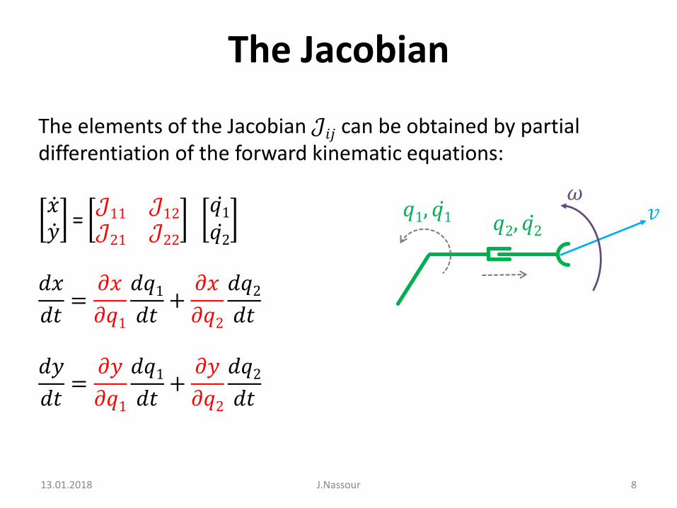
The elements of the Jacobian 𝒥𝑖𝑗 can be obtained by partial differentiation of the forward kinematic equations:
𝑥 𝑦
=𝒥11 𝒥12
𝒥21 𝒥22
𝑞1 𝑞2
𝑑𝑥
𝑑𝑡=
𝜕𝑥
𝜕𝑞1
𝑑𝑞1𝑑𝑡
+𝜕𝑥
𝜕𝑞2
𝑑𝑞2𝑑𝑡
𝑑𝑦
𝑑𝑡=
𝜕𝑦
𝜕𝑞1
𝑑𝑞1𝑑𝑡
+𝜕𝑦
𝜕𝑞2
𝑑𝑞2𝑑𝑡
𝑞2, 𝑞2𝑣
𝜔𝑞1, 𝑞1
13.01.2018 J.Nassour 8
The Jacobian
The elements of the Jacobian 𝒥𝑖𝑗 can be obtained by partial differentiation of the forward kinematic equations:
𝑥 𝑦
=𝒥11 𝒥12
𝒥21 𝒥22
𝑞1 𝑞2
𝑑𝑥
𝑑𝑡=
𝜕𝑥
𝜕𝑞1
𝑑𝑞1𝑑𝑡
+𝜕𝑥
𝜕𝑞2
𝑑𝑞2𝑑𝑡
𝑑𝑦
𝑑𝑡=
𝜕𝑦
𝜕𝑞1
𝑑𝑞1𝑑𝑡
+𝜕𝑦
𝜕𝑞2
𝑑𝑞2𝑑𝑡
𝑞2, 𝑞2𝑣
𝜔𝑞1, 𝑞1

13.01.2018 J.Nassour 9
The Jacobian
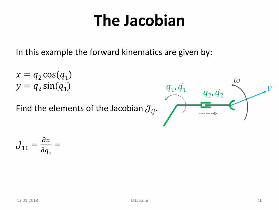
In this example the forward kinematics are given by:
𝑥 = 𝑞2 cos(𝑞1)𝑦 = 𝑞2 sin(𝑞1)
Find the elements of the Jacobian 𝒥𝑖𝑗.
𝑞2, 𝑞2𝑣
𝜔𝑞1, 𝑞1
13.01.2018 J.Nassour 10
The Jacobian
In this example the forward kinematics are given by:
𝑥 = 𝑞2 cos(𝑞1)𝑦 = 𝑞2 sin(𝑞1)
Find the elements of the Jacobian 𝒥𝑖𝑗.
𝒥11 =𝜕𝑥
𝜕𝑞1
= −𝑞2 sin(𝑞1) 𝒥12 =𝜕𝑥
𝜕𝑞2
= 𝑐𝑜𝑠(𝑞1)
𝒥21 =𝜕𝑦
𝜕𝑞1
= 𝑞2 cos(𝑞1) 𝒥22 =𝜕𝑦
𝜕𝑞2
= 𝑠𝑖𝑛(𝑞1)
This is the linear velocity Jacobian.
𝑞2, 𝑞2𝑣
𝜔𝑞1, 𝑞1

13.01.2018 J.Nassour 11
The Jacobian
In this example the forward kinematics are given by:
𝑥 = 𝑞2 cos(𝑞1)𝑦 = 𝑞2 sin(𝑞1)
Find the elements of the Jacobian 𝒥𝑖𝑗.
𝒥11 =𝜕𝑥
𝜕𝑞1
= −𝑞2 sin(𝑞1) 𝒥12 =𝜕𝑥
𝜕𝑞2
= 𝑐𝑜𝑠(𝑞1)
𝒥21 =𝜕𝑦
𝜕𝑞1
= 𝑞2 cos(𝑞1) 𝒥22 =𝜕𝑦
𝜕𝑞2
= 𝑠𝑖𝑛(𝑞1)
This is the linear velocity Jacobian.
𝑞2, 𝑞2𝑣
𝜔𝑞1, 𝑞1

13.01.2018 J.Nassour 12
The Jacobian
In this example the forward kinematics are given by:
𝑥 = 𝑞2 cos(𝑞1)𝑦 = 𝑞2 sin(𝑞1)
Find the elements of the Jacobian 𝒥𝑖𝑗.
𝒥11 =𝜕𝑥
𝜕𝑞1
= −𝑞2 sin(𝑞1) 𝒥12 =𝜕𝑥
𝜕𝑞2
= 𝑐𝑜𝑠(𝑞1)
𝒥21 =𝜕𝑦
𝜕𝑞1
= 𝑞2 cos(𝑞1) 𝒥22 =𝜕𝑦
𝜕𝑞2
= 𝑠𝑖𝑛(𝑞1)
This is the linear velocity Jacobian.
𝑞2, 𝑞2𝑣
𝜔𝑞1, 𝑞1

13.01.2018 J.Nassour 13
The Jacobian
In this example the forward kinematics are given by:
𝑥 = 𝑞2 cos(𝑞1)𝑦 = 𝑞2 sin(𝑞1)
Find the elements of the Jacobian 𝒥𝑖𝑗.
𝒥11 =𝜕𝑥
𝜕𝑞1
= −𝑞2 sin(𝑞1) 𝒥12 =𝜕𝑥
𝜕𝑞2
= 𝑐𝑜𝑠(𝑞1)
𝒥21 =𝜕𝑦
𝜕𝑞1
= 𝑞2 cos(𝑞1) 𝒥22 =𝜕𝑦
𝜕𝑞2
= 𝑠𝑖𝑛(𝑞1)
This is the linear velocity Jacobian.
𝑞2, 𝑞2𝑣
𝜔𝑞1, 𝑞1
13.01.2018 J.Nassour 14
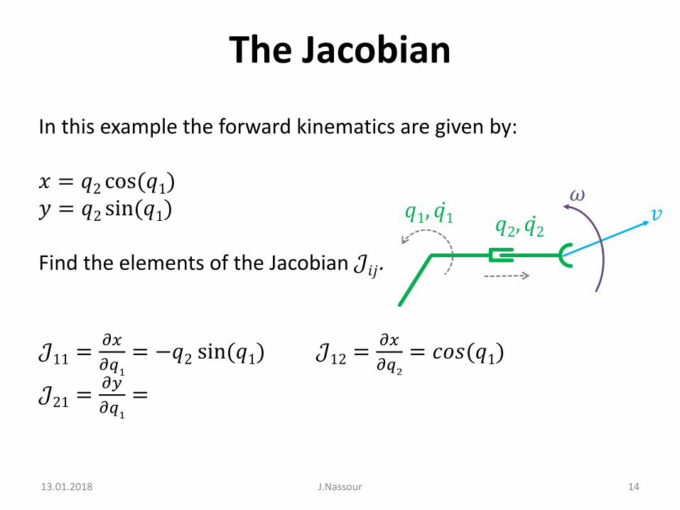
The Jacobian
In this example the forward kinematics are given by:
𝑥 = 𝑞2 cos(𝑞1)𝑦 = 𝑞2 sin(𝑞1)
Find the elements of the Jacobian 𝒥𝑖𝑗.
𝒥11 =𝜕𝑥
𝜕𝑞1
= −𝑞2 sin(𝑞1) 𝒥12 =𝜕𝑥
𝜕𝑞2
= 𝑐𝑜𝑠(𝑞1)
𝒥21 =𝜕𝑦
𝜕𝑞1
= 𝑞2 cos(𝑞1) 𝒥22 =𝜕𝑦
𝜕𝑞2
= 𝑠𝑖𝑛(𝑞1)
This is the linear velocity Jacobian.
𝑞2, 𝑞2𝑣
𝜔𝑞1, 𝑞1

13.01.2018 J.Nassour 15
The Jacobian
In this example the forward kinematics are given by:
𝑥 = 𝑞2 cos(𝑞1)𝑦 = 𝑞2 sin(𝑞1)
Find the elements of the Jacobian 𝒥𝑖𝑗.
𝒥11 =𝜕𝑥
𝜕𝑞1
= −𝑞2 sin(𝑞1) 𝒥12 =𝜕𝑥
𝜕𝑞2
= 𝑐𝑜𝑠(𝑞1)
𝒥21 =𝜕𝑦
𝜕𝑞1
= 𝑞2 cos(𝑞1) 𝒥22 =𝜕𝑦
𝜕𝑞2
= 𝑠𝑖𝑛(𝑞1)
This is the linear velocity Jacobian.
𝑞2, 𝑞2𝑣
𝜔𝑞1, 𝑞1

13.01.2018 J.Nassour 16
The Jacobian
In this example the forward kinematics are given by:
𝑥 = 𝑞2 cos(𝑞1)𝑦 = 𝑞2 sin(𝑞1)
Find the elements of the Jacobian 𝒥𝑖𝑗.
𝒥11 =𝜕𝑥
𝜕𝑞1
= −𝑞2 sin(𝑞1) 𝒥12 =𝜕𝑥
𝜕𝑞2
= 𝑐𝑜𝑠(𝑞1)
𝒥21 =𝜕𝑦
𝜕𝑞1
= 𝑞2 cos(𝑞1) 𝒥22 =𝜕𝑦
𝜕𝑞2
= 𝑠𝑖𝑛(𝑞1)
This is the linear velocity Jacobian.
𝑞2, 𝑞2𝑣
𝜔𝑞1, 𝑞1

13.01.2018 J.Nassour 17
The Jacobian
In this example the forward kinematics are given by:
𝑥 = 𝑞2 cos(𝑞1)𝑦 = 𝑞2 sin(𝑞1)
Find the elements of the Jacobian 𝒥𝑖𝑗.
𝒥11 =𝜕𝑥
𝜕𝑞1
= −𝑞2 sin(𝑞1) 𝒥12 =𝜕𝑥
𝜕𝑞2
= 𝑐𝑜𝑠(𝑞1)
𝒥21 =𝜕𝑦
𝜕𝑞1
= 𝑞2 cos(𝑞1) 𝒥22 =𝜕𝑦
𝜕𝑞2
= 𝑠𝑖𝑛(𝑞1)
This is the linear velocity Jacobian.
𝑞2, 𝑞2𝑣
𝜔𝑞1, 𝑞1
13.01.2018 J.Nassour 18
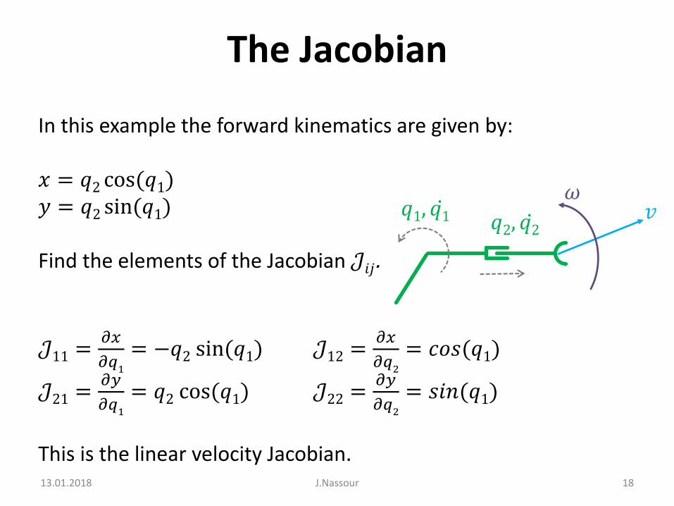
The Jacobian
In this example the forward kinematics are given by:
𝑥 = 𝑞2 cos(𝑞1)𝑦 = 𝑞2 sin(𝑞1)
Find the elements of the Jacobian 𝒥𝑖𝑗.
𝒥11 =𝜕𝑥
𝜕𝑞1
= −𝑞2 sin(𝑞1) 𝒥12 =𝜕𝑥
𝜕𝑞2
= 𝑐𝑜𝑠(𝑞1)
𝒥21 =𝜕𝑦
𝜕𝑞1
= 𝑞2 cos(𝑞1) 𝒥22 =𝜕𝑦
𝜕𝑞2
= 𝑠𝑖𝑛(𝑞1)
This is the linear velocity Jacobian.
𝑞2, 𝑞2𝑣
𝜔𝑞1, 𝑞1

13.01.2018 J.Nassour 19
The Jacobian
The angular velocity Jacobian:
𝑣𝜔
= 𝒥(𝑞1, 𝑞2) 𝑞1 𝑞2
For the angular velocity:
𝜔 = 𝒥𝜔 𝑞
𝜔 = 𝒥1 𝒥2
𝑞1 𝑞2
In this example: 𝒥1 = 1 , 𝒥2 = 0
𝑞2, 𝑞2𝑣
𝜔𝑞1, 𝑞1

13.01.2018 J.Nassour 20
The Jacobian
The angular velocity Jacobian:
𝑣𝜔
= 𝒥(𝑞1, 𝑞2) 𝑞1 𝑞2
For the angular velocity:
𝜔 = 𝒥𝜔 𝑞
𝜔 = 𝒥1 𝒥2
𝑞1 𝑞2
In this example: 𝒥1 = 1 , 𝒥2 = 0
𝑞2, 𝑞2𝑣
𝜔𝑞1, 𝑞1

13.01.2018 J.Nassour 21
The Jacobian
The angular velocity Jacobian:
𝑣𝜔
= 𝒥(𝑞1, 𝑞2) 𝑞1 𝑞2
For the angular velocity:
𝜔 = 𝒥𝜔 𝑞
𝜔 = 𝒥1 𝒥2
𝑞1 𝑞2
In this example: 𝒥1 = 1 , 𝒥2 = 0
𝑞2, 𝑞2𝑣
𝜔𝑞1, 𝑞1

13.01.2018 J.Nassour 22
Full Manipulator Jacobian
By combining the angular velocity Jacobian and the linear velocity Jacobian:
𝑣𝜔
= 𝒥(𝑞1, 𝑞2) 𝑞1 𝑞2
𝑥 𝑦𝜔
= −𝑞2 sin(𝑞1) cos(𝑞1)𝑞2 cos(𝑞1) sin(𝑞1)
1 0
𝑞1 𝑞2
The full Jacobian is an n×m matrix where n is the number of joints, and m is the number of variables describing motion.
𝑞2, 𝑞2𝑣
𝜔𝑞1, 𝑞1

13.01.2018 J.Nassour 23
Full Manipulator Jacobian
Work out the linear and the angular velocities, with joint 2 extendedto 0.5 m. The arm points in the x direction. Joint 1 is rotating at 2 rad/s and joint 2 is extending at 1 m/s.
𝑥 𝑦𝜔
= −𝑞2 sin(𝑞1) cos(𝑞1)𝑞2 cos(𝑞1) sin(𝑞1)
1 0
𝑞1 𝑞2
𝑞2, 𝑞2𝑣
𝜔𝑞1, 𝑞1
13.01.2018 J.Nassour 24
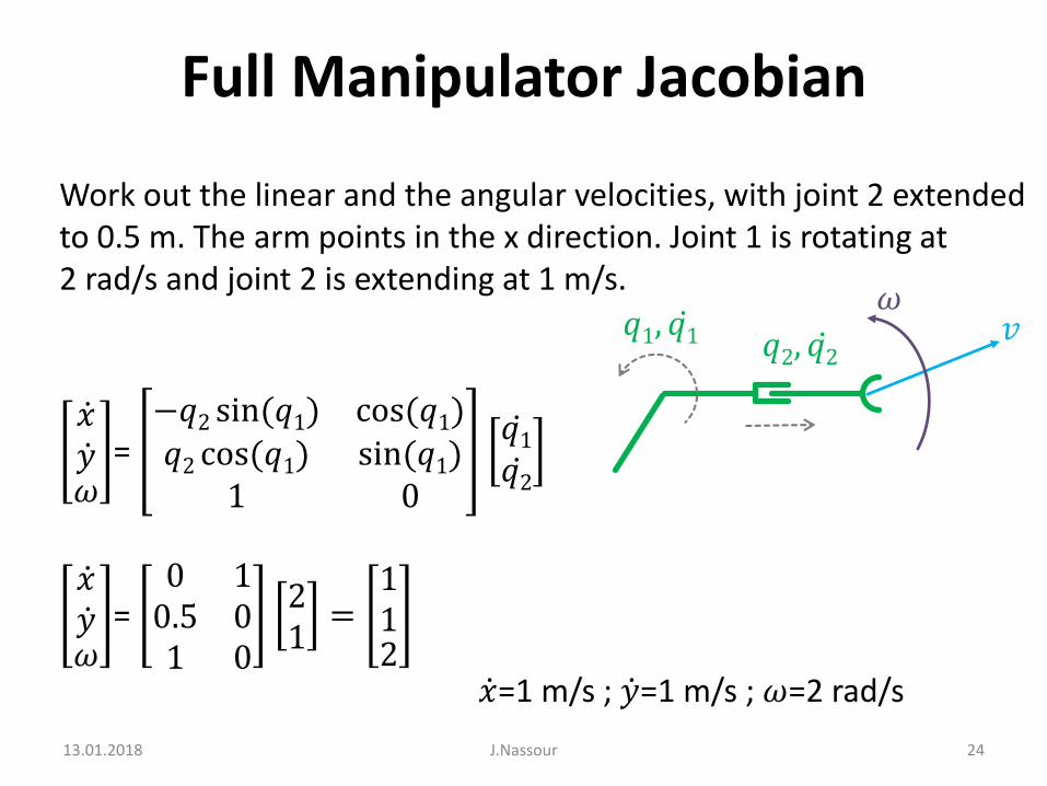
Full Manipulator Jacobian
Work out the linear and the angular velocities, with joint 2 extendedto 0.5 m. The arm points in the x direction. Joint 1 is rotating at 2 rad/s and joint 2 is extending at 1 m/s.
𝑥 𝑦𝜔
= −𝑞2 sin(𝑞1) cos(𝑞1)𝑞2 cos(𝑞1) sin(𝑞1)
1 0
𝑞1 𝑞2
𝑥 𝑦𝜔
= 0 10.5 01 0
21
=112
𝑥=1 m/s ; 𝑦=1 m/s ; 𝜔=2 rad/s
𝑞2, 𝑞2𝑣
𝜔𝑞1, 𝑞1

13.01.2018 J.Nassour 25
Inverting The Jacobian
To determine the joint velocities for a given end effector velocity, weneed to invert the Jacobian:
𝑣𝜔
= 𝒥 𝑞 𝑞
𝑞 = 𝒥−1 𝑞𝑣𝜔

13.01.2018 J.Nassour 26
Inverting The Jacobian
Find the joint velocities ( 𝑞1, 𝑞2) in terms of the end effector velocity ( 𝑥, 𝑦).
𝑥 𝑦
= −𝑞2 sin(𝑞1) cos(𝑞1)𝑞2 cos(𝑞1) sin(𝑞1)
𝑞1 𝑞2
𝑞1 𝑞2= 𝒥−1 𝑞
𝑥 𝑦
𝑞2, 𝑞2𝑣
𝜔𝑞1, 𝑞1

13.01.2018 J.Nassour 27
Inverting The Jacobian
Find the joint velocities ( 𝑞1, 𝑞2) in terms of the end effector velocity ( 𝑥, 𝑦).
𝑞1 𝑞2=
−𝑞2 sin(𝑞1) cos(𝑞1)𝑞2 cos(𝑞1) sin(𝑞1)
−1 𝑥 𝑦
𝑞1 𝑞2=
1
−𝑞2
sin(𝑞1) −cos(𝑞1)−𝑞2 cos(𝑞1) −𝑞2 sin(𝑞1)
𝑥 𝑦
𝑞2, 𝑞2𝑣
𝜔𝑞1, 𝑞1

13.01.2018 J.Nassour 28
Inverting The Jacobian
Find the joint velocities ( 𝑞1, 𝑞2) in terms of the end effector velocity ( 𝑥, 𝑦).
𝑞1 𝑞2=
−𝑞2 sin(𝑞1) cos(𝑞1)𝑞2 cos(𝑞1) sin(𝑞1)
−1 𝑥 𝑦
𝑞1 𝑞2=
1
−𝑞2
sin(𝑞1) −cos(𝑞1)−𝑞2 cos(𝑞1) −𝑞2 sin(𝑞1)
𝑥 𝑦
𝑞2, 𝑞2𝑣
𝜔𝑞1, 𝑞1

13.01.2018 J.Nassour 29
Inverting The Jacobian
Find the joint velocities ( 𝑞1, 𝑞2) in terms of the end effector velocity ( 𝑥, 𝑦).
𝑞1 𝑞2=
−𝑞2 sin(𝑞1) cos(𝑞1)𝑞2 cos(𝑞1) sin(𝑞1)
−1 𝑥 𝑦
𝑞1 𝑞2=
1
−𝑞2
sin(𝑞1) −cos(𝑞1)−𝑞2 cos(𝑞1) −𝑞2 sin(𝑞1)
𝑥 𝑦
𝑞2, 𝑞2𝑣
𝜔𝑞1, 𝑞1

13.01.2018 J.Nassour 30
Inverting The Jacobian
Find the joint velocities ( 𝑞1, 𝑞2) in terms of the end effector velocity ( 𝑥, 𝑦).
𝑞1 𝑞2=
−𝑞2 sin(𝑞1) cos(𝑞1)𝑞2 cos(𝑞1) sin(𝑞1)
−1 𝑥 𝑦
𝑞1 𝑞2=
1
−𝑞2
sin(𝑞1) −cos(𝑞1)−𝑞2 cos(𝑞1) −𝑞2 sin(𝑞1)
𝑥 𝑦
𝑞2, 𝑞2𝑣
𝜔𝑞1, 𝑞1

13.01.2018 J.Nassour 31
Inverting The Jacobian
Find the joint velocities ( 𝑞1, 𝑞2) in terms of the end effector velocity ( 𝑥, 𝑦).
𝑞1 𝑞2=
−𝑞2 sin(𝑞1) cos(𝑞1)𝑞2 cos(𝑞1) sin(𝑞1)
−1 𝑥 𝑦
𝑞1 𝑞2=
1
−𝑞2
sin(𝑞1) −cos(𝑞1)−𝑞2 cos(𝑞1) −𝑞2 sin(𝑞1)
𝑥 𝑦
𝑞2, 𝑞2𝑣
𝜔𝑞1, 𝑞1

13.01.2018 J.Nassour 32
Inverting The Jacobian
Find the joint velocities ( 𝑞1, 𝑞2) in terms of the end effector velocity ( 𝑥, 𝑦).
𝑞1 𝑞2=
−𝑞2 sin(𝑞1) cos(𝑞1)𝑞2 cos(𝑞1) sin(𝑞1)
−1 𝑥 𝑦
𝑞1 𝑞2=
1
−𝑞2
sin(𝑞1) −cos(𝑞1)−𝑞2 cos(𝑞1) −𝑞2 sin(𝑞1)
𝑥 𝑦
𝑞2, 𝑞2𝑣
𝜔𝑞1, 𝑞1

13.01.2018 J.Nassour 33
Inverting The Jacobian
𝑞1 𝑞2=
1
−𝑞2
sin(𝑞1) −cos(𝑞1)−𝑞2 cos(𝑞1) −𝑞2 sin(𝑞1)
𝑥 𝑦
The example arm points in the x Direction, with joint 2 extended to 0.5 m.
Find the joint velocities to move the end effector such that: 𝑥=1 m/s ; 𝑦=1 m/s
𝑞1= 2 rad/s ; 𝑞2= 1 m/s
𝑞2, 𝑞2𝑣
𝜔𝑞1, 𝑞1

13.01.2018 J.Nassour 34
Singularities
The effect of the determinant in the inverse Jacobian example:
𝑞1 𝑞2=
1
−𝑞2
sin(𝑞1) −cos(𝑞1)−𝑞2 cos(𝑞1) −𝑞2 sin(𝑞1)
𝑥 𝑦
Whenever 𝑞2= 0 m, there are no valid joint velocity solutions.
Limited end effector velocities give unlimited joint velocities.
𝑞2, 𝑞2𝑣
𝜔𝑞1, 𝑞1

13.01.2018 J.Nassour 35
Singularities
If the determinant of a square Jacobian is zero, the manipulator cannot be controlled.
• It is useful to observe the determinant of the Jacobian as the robot moves to avoid singularities.
• Avoid configuration where the determinant approaches zero.

13.01.2018 J.Nassour 36
Joint’s VelocityPrismatic Joint:
𝑣 = 𝑞𝑘𝝎 = 𝟎
Revolute Joint :
𝑣 = 𝑞𝑘 × 𝑟𝝎 = 𝒒𝒌
𝑘 is the unit vector.
𝑞𝑘 𝑣
𝑞
𝑘
𝑣
𝜔
𝑟

13.01.2018 J.Nassour 37
Angular Velocity
Prismatic joint gives 𝜔 = 0 and revolute joint gives 𝜔 = 𝑞𝑘
The general Jacobian for the angular velocity: 𝒥𝜔 = 𝜌1𝑧0 𝜌2𝑧1 … 𝜌𝑛𝑧𝑛 − 1
• 𝜌𝑖 is 1 if the joint is revolute and 0 if the joint is prismatic. • 𝑧𝑖is the direction of the z axis of the ith coordinate frame with
respect to the base frame.• 𝑧𝑖 is the first three elements of third column of the general
transformation matrix.
A1.A2…Ai = T0i =
𝑥𝑥 𝑦𝑥𝑥𝑦 𝑦𝑦
𝑧𝑥 𝑜𝑥𝑧𝑦 𝑜𝑦
𝑥𝑧 𝑦𝑧0 0
𝑧𝑧 𝑜𝑧0 1

Example: RRP Robot
13.01.2018
Find the angular velocity Jacobianfor the arm RRP.
Joint 3
Joint 1
Joint 2
Tool 𝒛𝟎
𝒙𝟎
𝒚𝟎
𝒛𝟏𝒙𝟏𝒚𝟏
𝒙𝟐
𝒚𝟐
𝒛𝟐
𝒛𝟑
𝒚𝟑
𝒙𝟑
𝑳3
3𝑚
J.Nassour 38
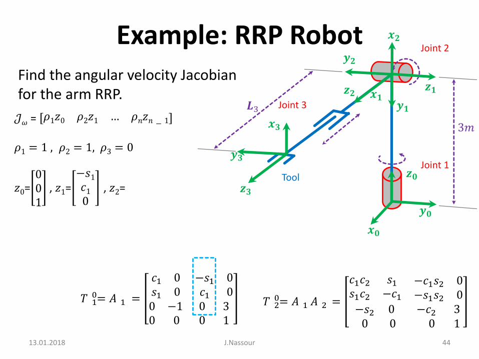
𝒥𝜔 = 𝜌1𝑧0 𝜌2𝑧1 … 𝜌𝑛𝑧𝑛 − 1
𝜌1 =? , 𝜌2 =?, 𝜌3 =?
𝑇 20= 𝐴 1 𝐴 2 =
𝑐1𝑐2 𝑠1𝑠1𝑐2 −𝑐1
−𝑐1𝑠2 0−𝑠1𝑠2 0
−𝑠2 00 0
−𝑐2 30 1
𝑇 10= 𝐴 1 =
𝑐1 0𝑠1 0
−𝑠1 0𝑐1 0
0 −10 0
0 30 1

Example: RRP Robot
13.01.2018
Find the angular velocity Jacobianfor the arm RRP.
Joint 3
Joint 1
Joint 2
Tool 𝒛𝟎
𝒙𝟎
𝒚𝟎
𝒛𝟏𝒙𝟏𝒚𝟏
𝒙𝟐
𝒚𝟐
𝒛𝟐
𝒛𝟑
𝒚𝟑
𝒙𝟑
𝑳3
3𝑚
J.Nassour 39
𝒥𝜔 = 𝜌1𝑧0 𝜌2𝑧1 … 𝜌𝑛𝑧𝑛 − 1
𝜌1 = 1 , 𝜌2 = 1, 𝜌3 = 0
𝑇 20= 𝐴 1 𝐴 2 =
𝑐1𝑐2 𝑠1𝑠1𝑐2 −𝑐1
−𝑐1𝑠2 0−𝑠1𝑠2 0
−𝑠2 00 0
−𝑐2 30 1
𝑇 10= 𝐴 1 =
𝑐1 0𝑠1 0
−𝑠1 0𝑐1 0
0 −10 0
0 30 1

Example: RRP Robot
13.01.2018
Find the angular velocity Jacobianfor the arm RRP.
Joint 3
Joint 1
Joint 2
Tool 𝒛𝟎
𝒙𝟎
𝒚𝟎
𝒛𝟏𝒙𝟏𝒚𝟏
𝒙𝟐
𝒚𝟐
𝒛𝟐
𝒛𝟑
𝒚𝟑
𝒙𝟑
𝑳3
3𝑚
J.Nassour 40
𝒥𝜔 = 𝜌1𝑧0 𝜌2𝑧1 … 𝜌𝑛𝑧𝑛 − 1
𝜌1 = 1 , 𝜌2 = 1, 𝜌3 = 0
𝑧0=001
, 𝑧1=−𝑠1𝑐10
, 𝑧2=
−𝑐1𝑠2−𝑠1𝑠2−𝑐2
𝑇 20= 𝐴 1 𝐴 2 =
𝑐1𝑐2 𝑠1𝑠1𝑐2 −𝑐1
−𝑐1𝑠2 0−𝑠1𝑠2 0
−𝑠2 00 0
−𝑐2 30 1
𝑇 10= 𝐴 1 =
𝑐1 0𝑠1 0
−𝑠1 0𝑐1 0
0 −10 0
0 30 1

Example: RRP Robot
13.01.2018
Find the angular velocity Jacobianfor the arm RRP.
Joint 3
Joint 1
Joint 2
Tool 𝒛𝟎
𝒙𝟎
𝒚𝟎
𝒛𝟏𝒙𝟏𝒚𝟏
𝒙𝟐
𝒚𝟐
𝒛𝟐
𝒛𝟑
𝒚𝟑
𝒙𝟑
𝑳3
3𝑚
J.Nassour 41
𝒥𝜔 = 𝜌1𝑧0 𝜌2𝑧1 … 𝜌𝑛𝑧𝑛 − 1
𝜌1 = 1 , 𝜌2 = 1, 𝜌3 = 0
𝑧0=001
, 𝑧1=−𝑠1𝑐10
, 𝑧2=
−𝑐1𝑠2−𝑠1𝑠2−𝑐2
𝑇 20= 𝐴 1 𝐴 2 =
𝑐1𝑐2 𝑠1𝑠1𝑐2 −𝑐1
−𝑐1𝑠2 0−𝑠1𝑠2 0
−𝑠2 00 0
−𝑐2 30 1
𝑇 10= 𝐴 1 =
𝑐1 0𝑠1 0
−𝑠1 0𝑐1 0
0 −10 0
0 30 1

Example: RRP Robot
13.01.2018
Find the angular velocity Jacobianfor the arm RRP.
Joint 3
Joint 1
Joint 2
Tool 𝒛𝟎
𝒙𝟎
𝒚𝟎
𝒛𝟏𝒙𝟏𝒚𝟏
𝒙𝟐
𝒚𝟐
𝒛𝟐
𝒛𝟑
𝒚𝟑
𝒙𝟑
𝑳3
3𝑚
J.Nassour 42
𝒥𝜔 = 𝜌1𝑧0 𝜌2𝑧1 … 𝜌𝑛𝑧𝑛 − 1
𝜌1 = 1 , 𝜌2 = 1, 𝜌3 = 0
𝑧0=001
, 𝑧1=−𝑠1𝑐10
, 𝑧2=
−𝑐1𝑠2−𝑠1𝑠2−𝑐2
𝑇 20= 𝐴 1 𝐴 2 =
𝑐1𝑐2 𝑠1𝑠1𝑐2 −𝑐1
−𝑐1𝑠2 0−𝑠1𝑠2 0
−𝑠2 00 0
−𝑐2 30 1
𝑇 10= 𝐴 1 =
𝑐1 0𝑠1 0
−𝑠1 0𝑐1 0
0 −10 0
0 30 1

Example: RRP Robot
13.01.2018
Find the angular velocity Jacobianfor the arm RRP.
Joint 3
Joint 1
Joint 2
Tool 𝒛𝟎
𝒙𝟎
𝒚𝟎
𝒛𝟏𝒙𝟏𝒚𝟏
𝒙𝟐
𝒚𝟐
𝒛𝟐
𝒛𝟑
𝒚𝟑
𝒙𝟑
𝑳3
3𝑚
J.Nassour 43
𝒥𝜔 = 𝜌1𝑧0 𝜌2𝑧1 … 𝜌𝑛𝑧𝑛 − 1
𝜌1 = 1 , 𝜌2 = 1, 𝜌3 = 0
𝑧0=001
, 𝑧1=−𝑠1𝑐10
, 𝑧2=
−𝑐1𝑠2−𝑠1𝑠2−𝑐2
𝑇 20= 𝐴 1 𝐴 2 =
𝑐1𝑐2 𝑠1𝑠1𝑐2 −𝑐1
−𝑐1𝑠2 0−𝑠1𝑠2 0
−𝑠2 00 0
−𝑐2 30 1
𝑇 10= 𝐴 1 =
𝑐1 0𝑠1 0
−𝑠1 0𝑐1 0
0 −10 0
0 30 1
Example: RRP Robot
13.01.2018
Find the angular velocity Jacobianfor the arm RRP.
Joint 3
Joint 1
Joint 2
Tool 𝒛𝟎
𝒙𝟎
𝒚𝟎
𝒛𝟏𝒙𝟏𝒚𝟏
𝒙𝟐
𝒚𝟐
𝒛𝟐
𝒛𝟑
𝒚𝟑
𝒙𝟑
𝑳3
3𝑚
J.Nassour 44
𝒥𝜔 = 𝜌1𝑧0 𝜌2𝑧1 … 𝜌𝑛𝑧𝑛 − 1
𝜌1 = 1 , 𝜌2 = 1, 𝜌3 = 0
𝑧0=001
, 𝑧1=−𝑠1𝑐10
, 𝑧2=
−𝑐1𝑠2−𝑠1𝑠2−𝑐2
𝑇 20= 𝐴 1 𝐴 2 =
𝑐1𝑐2 𝑠1𝑠1𝑐2 −𝑐1
−𝑐1𝑠2 0−𝑠1𝑠2 0
−𝑠2 00 0
−𝑐2 30 1
𝑇 10= 𝐴 1 =
𝑐1 0𝑠1 0
−𝑠1 0𝑐1 0
0 −10 0
0 30 1

Example: RRP Robot
13.01.2018
Find the angular velocity Jacobianfor the arm RRP.
Joint 3
Joint 1
Joint 2
Tool 𝒛𝟎
𝒙𝟎
𝒚𝟎
𝒛𝟏𝒙𝟏𝒚𝟏
𝒙𝟐
𝒚𝟐
𝒛𝟐
𝒛𝟑
𝒚𝟑
𝒙𝟑
𝑳3
3𝑚
J.Nassour 45
𝒥𝜔 = 𝜌1𝑧0 𝜌2𝑧1 … 𝜌𝑛𝑧𝑛 − 1
𝜌1 = 1 , 𝜌2 = 1, 𝜌3 = 0
𝑧0=001
, 𝑧1=−𝑠1𝑐10
, 𝑧2=
−𝑐1𝑠2−𝑠1𝑠2−𝑐2
𝑇 20= 𝐴 1 𝐴 2 =
𝑐1𝑐2 𝑠1𝑠1𝑐2 −𝑐1
−𝑐1𝑠2 0−𝑠1𝑠2 0
−𝑠2 00 0
−𝑐2 30 1
𝑇 10= 𝐴 1 =
𝑐1 0𝑠1 0
−𝑠1 0𝑐1 0
0 −10 0
0 30 1

Example: RRP Robot
13.01.2018
Find the angular velocity Jacobianfor the arm RRP.
Joint 3
Joint 1
Joint 2
Tool 𝒛𝟎
𝒙𝟎
𝒚𝟎
𝒛𝟏𝒙𝟏𝒚𝟏
𝒙𝟐
𝒚𝟐
𝒛𝟐
𝒛𝟑
𝒚𝟑
𝒙𝟑
𝑳3
3𝑚
J.Nassour 46
𝒥𝜔 = 001
−𝑠1𝑐10
000
𝒥𝜔 = 𝜌1𝑧0 𝜌2𝑧1 … 𝜌𝑛𝑧𝑛 − 1
𝜌1 = 1 , 𝜌2 = 1, 𝜌3 = 0
𝑧0=001
, 𝑧1=−𝑠1𝑐10
, 𝑧2=
−𝑐1𝑠2−𝑠1𝑠2−𝑐2

Example: RRP Robot
13.01.2018
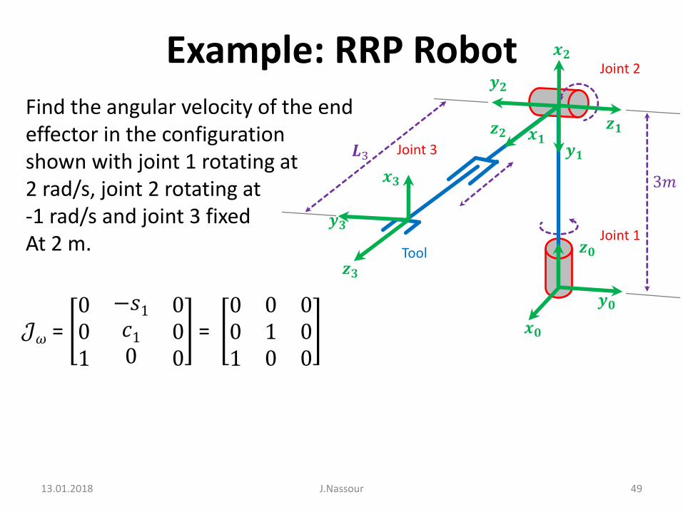
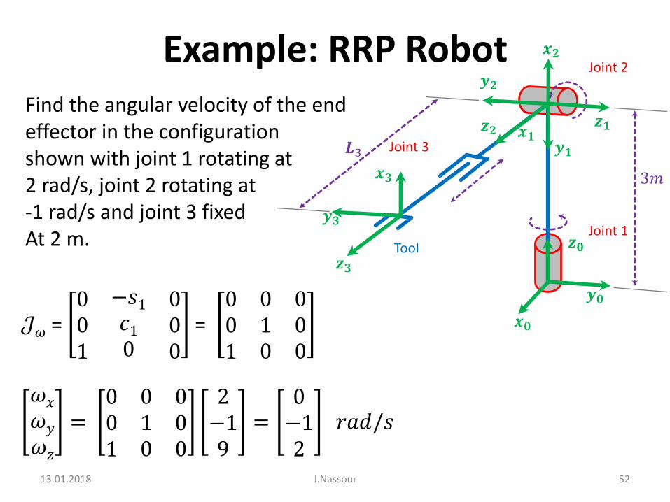
Find the angular velocity of the endeffector in the configuration shown with joint 1 rotating at 2 rad/s, joint 2 rotating at -1 rad/s and joint 3 fixedAt 2 m.
Joint 3
Joint 1
Joint 2
Tool 𝒛𝟎
𝒙𝟎
𝒚𝟎
𝒛𝟏𝒙𝟏𝒚𝟏
𝒙𝟐
𝒚𝟐
𝒛𝟐
𝒛𝟑
𝒚𝟑
𝒙𝟑
𝑳3
3𝑚
J.Nassour 47

Example: RRP Robot
13.01.2018
Find the angular velocity of the endeffector in the configuration shown with joint 1 rotating at 2 rad/s, joint 2 rotating at -1 rad/s and joint 3 fixedAt 2 m.
Joint 3
Joint 1
Joint 2
Tool 𝒛𝟎
𝒙𝟎
𝒚𝟎
𝒛𝟏𝒙𝟏𝒚𝟏
𝒙𝟐
𝒚𝟐
𝒛𝟐
𝒛𝟑
𝒚𝟑
𝒙𝟑
𝑳3
3𝑚
J.Nassour 48
𝒥𝜔 = 001
−𝑠1𝑐10
000
= 001
010
000
𝜔𝑥
𝜔𝑦
𝜔𝑧
=001
010
000
2−19
=0−12
𝑟𝑎𝑑/𝑠
The end effector is rotating 0 rad/s around x axis, -1 rad/s around y axis, and 2 rad/s around z axis.
Example: RRP Robot
13.01.2018
Find the angular velocity of the endeffector in the configuration shown with joint 1 rotating at 2 rad/s, joint 2 rotating at -1 rad/s and joint 3 fixedAt 2 m.
Joint 3
Joint 1
Joint 2
Tool 𝒛𝟎
𝒙𝟎
𝒚𝟎
𝒛𝟏𝒙𝟏𝒚𝟏
𝒙𝟐
𝒚𝟐
𝒛𝟐
𝒛𝟑
𝒚𝟑
𝒙𝟑
𝑳3
3𝑚
J.Nassour 49
𝒥𝜔 = 001
−𝑠1𝑐10
000
= 001
010
000
𝜔𝑥
𝜔𝑦
𝜔𝑧
=001
010
000
2−19
=0−12
𝑟𝑎𝑑/𝑠
The end effector is rotating 0 rad/s around x axis, -1 rad/s around y axis, and 2 rad/s around z axis.

Example: RRP Robot
13.01.2018
Find the angular velocity of the endeffector in the configuration shown with joint 1 rotating at 2 rad/s, joint 2 rotating at -1 rad/s and joint 3 fixedAt 2 m.
Joint 3
Joint 1
Joint 2
Tool 𝒛𝟎
𝒙𝟎
𝒚𝟎
𝒛𝟏𝒙𝟏𝒚𝟏
𝒙𝟐
𝒚𝟐
𝒛𝟐
𝒛𝟑
𝒚𝟑
𝒙𝟑
𝑳3
3𝑚
J.Nassour 50
𝒥𝜔 = 001
−𝑠1𝑐10
000
= 001
010
000
𝜔𝑥
𝜔𝑦
𝜔𝑧
=001
010
000
2−19
=0−12
𝑟𝑎𝑑/𝑠
The end effector is rotating 0 rad/s around x axis, -1 rad/s around y axis, and 2 rad/s around z axis.

Example: RRP Robot
13.01.2018
Find the angular velocity of the endeffector in the configuration shown with joint 1 rotating at 2 rad/s, joint 2 rotating at -1 rad/s and joint 3 fixedAt 2 m.
Joint 3
Joint 1
Joint 2
Tool 𝒛𝟎
𝒙𝟎
𝒚𝟎
𝒛𝟏𝒙𝟏𝒚𝟏
𝒙𝟐
𝒚𝟐
𝒛𝟐
𝒛𝟑
𝒚𝟑
𝒙𝟑
𝑳3
3𝑚
J.Nassour 51
𝒥𝜔 = 001
−𝑠1𝑐10
000
= 001
010
000
𝜔𝑥
𝜔𝑦
𝜔𝑧
=001
010
000
2−10
=0−12
𝑟𝑎𝑑/𝑠
The end effector is rotating 0 rad/s around x axis, -1 rad/s around y axis, and 2 rad/s around z axis.
Example: RRP Robot
13.01.2018
Find the angular velocity of the endeffector in the configuration shown with joint 1 rotating at 2 rad/s, joint 2 rotating at -1 rad/s and joint 3 fixedAt 2 m.
Joint 3
Joint 1
Joint 2
Tool 𝒛𝟎
𝒙𝟎
𝒚𝟎
𝒛𝟏𝒙𝟏𝒚𝟏
𝒙𝟐
𝒚𝟐
𝒛𝟐
𝒛𝟑
𝒚𝟑
𝒙𝟑
𝑳3
3𝑚
J.Nassour 52
𝒥𝜔 = 001
−𝑠1𝑐10
000
= 001
010
000
𝜔𝑥
𝜔𝑦
𝜔𝑧
=001
010
000
2−19
=0−12
𝑟𝑎𝑑/𝑠
The end effector is rotating 0 rad/s around x axis, -1 rad/s around y axis, and 2 rad/s around z axis.

Example: RRP Robot
13.01.2018
Find the angular velocity of the endeffector in the configuration shown with joint 1 rotating at 2 rad/s, joint 2 rotating at -1 rad/s and joint 3 fixedAt 2 m.
Joint 3
Joint 1
Joint 2
Tool 𝒛𝟎
𝒙𝟎
𝒚𝟎
𝒛𝟏𝒙𝟏𝒚𝟏
𝒙𝟐
𝒚𝟐
𝒛𝟐
𝒛𝟑
𝒚𝟑
𝒙𝟑
𝑳3
3𝑚
J.Nassour 53
𝒥𝜔 = 001
−𝑠1𝑐10
000
= 001
010
000
𝜔𝑥
𝜔𝑦
𝜔𝑧
=001
010
000
2−19
=0−12
𝑟𝑎𝑑/𝑠
The end effector is rotating 0 rad/s around x axis, -1 rad/s around y axis, and 2 rad/s around z axis.

Example: RRR Robot
13.01.2018
Find the angular velocity of the end effector in the configuration shown with joint 1 rotating at 2 rad/s, joint 2 rotating at -1 rad/s and joint 3 rotating at 2 rad/s.
“This is a typical example that can be discussed in the oral exam”
J.Nassour 54
Link 0 (fixed)
Joint 1
Link 1
Joint variable 𝜽1
Joint 2
Link 2
Joint variable 𝜽2
Link 3
𝒛𝟐
Joint 3
Joint variable 𝜽3
𝒛𝟑
𝒙𝟎
𝒚𝟎
𝒛𝟎
𝒛𝟏 𝒙𝟏
𝒚𝟏
𝒙𝟐
𝒚𝟐
𝒙𝟑
𝒚𝟑
Link 1= 2 mLink 2= 2 mLink 3= 2 m

Linear Velocity Jacobian
13.01.2018
The velocity of the end effector for an n link manipulator is the race of change of the origin of the end effector frame with respect to the base frame.
𝑜𝑛0 =
𝑖=1
𝑛𝜕𝑜𝑛
0
𝜕𝑞𝑖 𝑞𝑖
J.Nassour 55

The Origin 𝑜𝑖0
13.01.2018
The origin of the ith reference frame
𝑇𝑖0 =
𝑟11 𝑟12𝑟21 𝑟22
𝑟13 𝑜𝑥𝑟23 𝑜𝑦
𝑟31 𝑟320 0
𝑟33 𝑜𝑧0 1
J.Nassour 56

Linear Velocity Jacobian
13.01.2018
𝑜𝑛0 =
𝑖=1
𝑛𝜕𝑜𝑛
0
𝜕𝑞𝑖 𝑞𝑖
The contribution of each joint in the linear velocity of the end effector.
𝒥𝑣𝑖=𝜕𝑜𝑛
0
𝜕𝑞𝑖
Each column in the Jacobian is the rate of changes of the end effector in the base reference frame with respect to the rate of change of a joint variable qi.The ith column shows the movement of the end effector caused by 𝑞𝑖.
J.Nassour 57

Prismatic Joint
13.01.2018
Displacement along the axis of actuation 𝑧𝑖−1:
𝑜𝑛0 = 𝑑𝑖𝑧𝑖−1
0
𝑣 = 𝑧𝑖−10 𝑞𝑖
𝓙𝒗𝒊= 𝒛𝒊−𝟏
𝟎
J.Nassour 58
End effectorVelocity
Joint Velocity

Revolute Joint
13.01.2018
Displacement around the axis of actuation 𝑧𝑖−1:
𝑜𝑛0 = 𝜔 × 𝑟
𝑜𝑛0 = 𝑞𝑖 𝑧𝑖−1
0 × 𝑜𝑛 − 𝑜𝑖−1
𝑣 = 𝑧𝑖−10 × 𝑜𝑛 − 𝑜𝑖−1 𝑞𝑖
𝓙𝒗𝒊= 𝒛𝒊−𝟏
𝟎 × 𝒐𝒏 − 𝒐𝒊−𝟏
J.Nassour 59
End effectorVelocity
Joint Velocity

Example: RRP Robot
13.01.2018
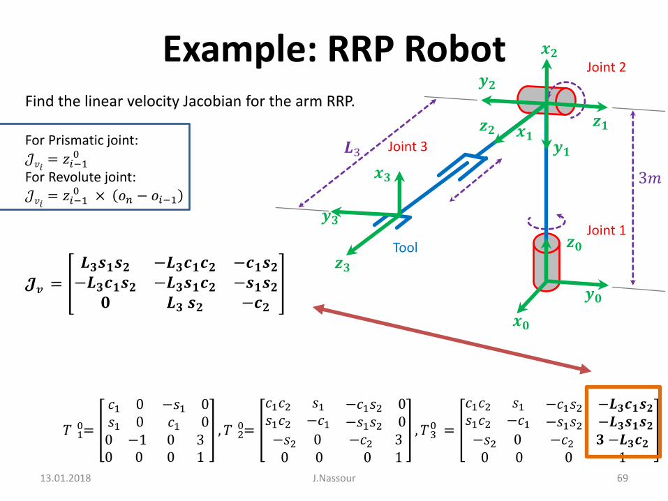
Find the linear velocity Jacobian for the arm RRP.
Joint 3
Joint 1
Joint 2
Tool 𝒛𝟎
𝒙𝟎
𝒚𝟎
𝒛𝟏𝒙𝟏𝒚𝟏
𝒙𝟐
𝒚𝟐
𝒛𝟐
𝒛𝟑
𝒚𝟑
𝒙𝟑
𝑳3
3𝑚
J.Nassour 60
𝑇 10=
𝑐1 0𝑠1 0
−𝑠1 0𝑐1 0
0 −10 0
0 30 1
, 𝑇 20=
𝑐1𝑐2 𝑠1𝑠1𝑐2 −𝑐1
−𝑐1𝑠2 0−𝑠1𝑠2 0
−𝑠2 00 0
−𝑐2 30 1
, 𝑇30 =
𝑐1𝑐2 𝑠1𝑠1𝑐2 −𝑐1
−𝑐1𝑠2 −𝐿𝟑𝑐1𝑠2−𝑠1𝑠2 −𝐿𝟑𝑠1𝑠2
−𝑠2 00 0
−𝑐2 3 −𝐿𝟑𝑐20 1

Example: RRP Robot
13.01.2018
Find the linear velocity Jacobian for the arm RRP.
For Prismatic joint:
𝒥𝑣𝑖= 𝑧𝑖−1
0
For Revolute joint:
𝒥𝑣𝑖= 𝑧𝑖−1
0 × 𝑜𝑛 − 𝑜𝑖−1
Joint 3
Joint 1
Joint 2
Tool 𝒛𝟎
𝒙𝟎
𝒚𝟎
𝒛𝟏𝒙𝟏𝒚𝟏
𝒙𝟐
𝒚𝟐
𝒛𝟐
𝒛𝟑
𝒚𝟑
𝒙𝟑
𝑳3
3𝑚
J.Nassour 61
𝑇 10=
𝑐1 0𝑠1 0
−𝑠1 0𝑐1 0
0 −10 0
0 30 1
, 𝑇 20=
𝑐1𝑐2 𝑠1𝑠1𝑐2 −𝑐1
−𝑐1𝑠2 0−𝑠1𝑠2 0
−𝑠2 00 0
−𝑐2 30 1
, 𝑇30 =
𝑐1𝑐2 𝑠1𝑠1𝑐2 −𝑐1
−𝑐1𝑠2 −𝐿𝟑𝑐1𝑠2−𝑠1𝑠2 −𝐿𝟑𝑠1𝑠2
−𝑠2 00 0
−𝑐2 3 −𝐿𝟑𝑐20 1

Example: RRP Robot
13.01.2018
Find the linear velocity Jacobian for the arm RRP.
For Prismatic joint:
𝒥𝑣𝑖= 𝑧𝑖−1
0
For Revolute joint:
𝒥𝑣𝑖= 𝑧𝑖−1
0 × 𝑜𝑛 − 𝑜𝑖−1
𝒥𝑣1= 𝑧0
0 × 𝑜3 − 𝑜0
𝒥𝑣1=
001
×
−𝐿𝟑𝑐1𝑠2 − 0−𝐿𝟑𝑠1𝑠2 − 03 −𝐿𝟑𝑐2 − 0
=𝐿𝟑𝑠1𝑠2−𝐿𝟑𝑐1𝑠2
0
Joint 3
Joint 1
Joint 2
Tool 𝒛𝟎
𝒙𝟎
𝒚𝟎
𝒛𝟏𝒙𝟏𝒚𝟏
𝒙𝟐
𝒚𝟐
𝒛𝟐
𝒛𝟑
𝒚𝟑
𝒙𝟑
𝑳3
3𝑚
J.Nassour 62
𝑇 10=
𝑐1 0𝑠1 0
−𝑠1 0𝑐1 0
0 −10 0
0 30 1
, 𝑇 20=
𝑐1𝑐2 𝑠1𝑠1𝑐2 −𝑐1
−𝑐1𝑠2 0−𝑠1𝑠2 0
−𝑠2 00 0
−𝑐2 30 1
, 𝑇30 =
𝑐1𝑐2 𝑠1𝑠1𝑐2 −𝑐1
−𝑐1𝑠2 −𝐿𝟑𝑐1𝑠2−𝑠1𝑠2 −𝐿𝟑𝑠1𝑠2
−𝑠2 00 0
−𝑐2 3 −𝐿𝟑𝑐20 1

Example: RRP Robot
13.01.2018
Find the linear velocity Jacobian for the arm RRP.
For Prismatic joint:
𝒥𝑣𝑖= 𝑧𝑖−1
0
For Revolute joint:
𝒥𝑣𝑖= 𝑧𝑖−1
0 × 𝑜𝑛 − 𝑜𝑖−1
𝒥𝑣1= 𝑧0
0 × 𝑜3 − 𝑜0
𝒥𝑣1=
001
×
−𝐿𝟑𝑐1𝑠2 − 0−𝐿𝟑𝑠1𝑠2 − 03 −𝐿𝟑𝑐2 − 0
=𝐿𝟑𝑠1𝑠2−𝐿𝟑𝑐1𝑠2
0
Joint 3
Joint 1
Joint 2
Tool 𝒛𝟎
𝒙𝟎
𝒚𝟎
𝒛𝟏𝒙𝟏𝒚𝟏
𝒙𝟐
𝒚𝟐
𝒛𝟐
𝒛𝟑
𝒚𝟑
𝒙𝟑
𝑳3
3𝑚
J.Nassour 63
𝑇 10=
𝑐1 0𝑠1 0
−𝑠1 0𝑐1 0
0 −10 0
0 30 1
, 𝑇 20=
𝑐1𝑐2 𝑠1𝑠1𝑐2 −𝑐1
−𝑐1𝑠2 0−𝑠1𝑠2 0
−𝑠2 00 0
−𝑐2 30 1
, 𝑇30 =
𝑐1𝑐2 𝑠1𝑠1𝑐2 −𝑐1
−𝑐1𝑠2 −𝐿𝟑𝑐1𝑠2−𝑠1𝑠2 −𝐿𝟑𝑠1𝑠2
−𝑠2 00 0
−𝑐2 3 −𝐿𝟑𝑐20 1

Example: RRP Robot
13.01.2018
Find the linear velocity Jacobian for the arm RRP.
For Prismatic joint:
𝒥𝑣𝑖= 𝑧𝑖−1
0
For Revolute joint:
𝒥𝑣𝑖= 𝑧𝑖−1
0 × 𝑜𝑛 − 𝑜𝑖−1
𝒥𝑣2= 𝑧1
0 × 𝑜3 − 𝑜1
𝒥𝑣2=
−𝑠1𝑐10
×
−𝐿𝟑𝑐1𝑠2−𝐿𝟑𝑠1𝑠2−𝐿𝟑𝑐2
=
−𝐿𝟑𝑐1𝑐2−𝐿𝟑𝑠1𝑐2
𝐿3𝑠12 𝑠2 + 𝐿3𝑐1
2 𝑠2
=
−𝐿𝟑𝑐1𝑐2−𝐿𝟑𝑠1𝑐2𝐿3 𝑠2
Joint 3
Joint 1
Joint 2
Tool 𝒛𝟎
𝒙𝟎
𝒚𝟎
𝒛𝟏𝒙𝟏𝒚𝟏
𝒙𝟐
𝒚𝟐
𝒛𝟐
𝒛𝟑
𝒚𝟑
𝒙𝟑
𝑳3
3𝑚
J.Nassour 64
𝑇 10=
𝑐1 0𝑠1 0
−𝑠1 0𝑐1 0
0 −10 0
0 30 1
, 𝑇 20=
𝑐1𝑐2 𝑠1𝑠1𝑐2 −𝑐1
−𝑐1𝑠2 0−𝑠1𝑠2 0
−𝑠2 00 0
−𝑐2 30 1
, 𝑇30 =
𝑐1𝑐2 𝑠1𝑠1𝑐2 −𝑐1
−𝑐1𝑠2 −𝐿𝟑𝑐1𝑠2−𝑠1𝑠2 −𝐿𝟑𝑠1𝑠2
−𝑠2 00 0
−𝑐2 3 −𝐿𝟑𝑐20 1

Example: RRP Robot
13.01.2018
Find the linear velocity Jacobian for the arm RRP.
For Prismatic joint:
𝒥𝑣𝑖= 𝑧𝑖−1
0
For Revolute joint:
𝒥𝑣𝑖= 𝑧𝑖−1
0 × 𝑜𝑛 − 𝑜𝑖−1
𝒥𝑣2= 𝑧1
0 × 𝑜3 − 𝑜1
𝒥𝑣2=
−𝑠1𝑐10
×
−𝐿𝟑𝑐1𝑠2−𝐿𝟑𝑠1𝑠2−𝐿𝟑𝑐2
=
−𝐿𝟑𝑐1𝑐2−𝐿𝟑𝑠1𝑐2
𝐿3𝑠12 𝑠2 + 𝐿3𝑐1
2 𝑠2
=
−𝐿𝟑𝑐1𝑐2−𝐿𝟑𝑠1𝑐2𝐿3 𝑠2
Joint 3
Joint 1
Joint 2
Tool 𝒛𝟎
𝒙𝟎
𝒚𝟎
𝒛𝟏𝒙𝟏𝒚𝟏
𝒙𝟐
𝒚𝟐
𝒛𝟐
𝒛𝟑
𝒚𝟑
𝒙𝟑
𝑳3
3𝑚
J.Nassour 65
𝑇 10=
𝑐1 0𝑠1 0
−𝑠1 0𝑐1 0
0 −10 0
0 30 1
, 𝑇 20=
𝑐1𝑐2 𝑠1𝑠1𝑐2 −𝑐1
−𝑐1𝑠2 0−𝑠1𝑠2 0
−𝑠2 00 0
−𝑐2 30 1
, 𝑇30 =
𝑐1𝑐2 𝑠1𝑠1𝑐2 −𝑐1
−𝑐1𝑠2 −𝐿𝟑𝑐1𝑠2−𝑠1𝑠2 −𝐿𝟑𝑠1𝑠2
−𝑠2 00 0
−𝑐2 3 −𝐿𝟑𝑐20 1

Example: RRP Robot
13.01.2018
Find the linear velocity Jacobian for the arm RRP.
For Prismatic joint:
𝒥𝑣𝑖= 𝑧𝑖−1
0
For Revolute joint:
𝒥𝑣𝑖= 𝑧𝑖−1
0 × 𝑜𝑛 − 𝑜𝑖−1
𝒥𝑣3= 𝑧2
0
𝒥𝑣3=
−𝑐1𝑠2−𝑠1𝑠2−𝑐2
Joint 3
Joint 1
Joint 2
Tool 𝒛𝟎
𝒙𝟎
𝒚𝟎
𝒛𝟏𝒙𝟏𝒚𝟏
𝒙𝟐
𝒚𝟐
𝒛𝟐
𝒛𝟑
𝒚𝟑
𝒙𝟑
𝑳3
3𝑚
J.Nassour 66
𝑇 10=
𝑐1 0𝑠1 0
−𝑠1 0𝑐1 0
0 −10 0
0 30 1
, 𝑇 20=
𝑐1𝑐2 𝑠1𝑠1𝑐2 −𝑐1
−𝑐1𝑠2 0−𝑠1𝑠2 0
−𝑠2 00 0
−𝑐2 30 1
, 𝑇30 =
𝑐1𝑐2 𝑠1𝑠1𝑐2 −𝑐1
−𝑐1𝑠2 −𝐿𝟑𝑐1𝑠2−𝑠1𝑠2 −𝐿𝟑𝑠1𝑠2
−𝑠2 00 0
−𝑐2 3 −𝐿𝟑𝑐20 1

Example: RRP Robot
13.01.2018
Find the linear velocity Jacobian for the arm RRP.
For Prismatic joint:
𝒥𝑣𝑖= 𝑧𝑖−1
0
For Revolute joint:
𝒥𝑣𝑖= 𝑧𝑖−1
0 × 𝑜𝑛 − 𝑜𝑖−1
𝒥𝑣3= 𝑧2
0
𝒥𝑣3=
−𝑐1𝑠2−𝑠1𝑠2−𝑐2
Joint 3
Joint 1
Joint 2
Tool 𝒛𝟎
𝒙𝟎
𝒚𝟎
𝒛𝟏𝒙𝟏𝒚𝟏
𝒙𝟐
𝒚𝟐
𝒛𝟐
𝒛𝟑
𝒚𝟑
𝒙𝟑
𝑳3
3𝑚
J.Nassour 67
𝑇 10=
𝑐1 0𝑠1 0
−𝑠1 0𝑐1 0
0 −10 0
0 30 1
, 𝑇 20=
𝑐1𝑐2 𝑠1𝑠1𝑐2 −𝑐1
−𝑐1𝑠2 0−𝑠1𝑠2 0
−𝑠2 00 0
−𝑐2 30 1
, 𝑇30 =
𝑐1𝑐2 𝑠1𝑠1𝑐2 −𝑐1
−𝑐1𝑠2 −𝐿𝟑𝑐1𝑠2−𝑠1𝑠2 −𝐿𝟑𝑠1𝑠2
−𝑠2 00 0
−𝑐2 3 −𝐿𝟑𝑐20 1

Example: RRP Robot
13.01.2018
Find the linear velocity Jacobian for the arm RRP.
For Prismatic joint:
𝒥𝑣𝑖= 𝑧𝑖−1
0
For Revolute joint:
𝒥𝑣𝑖= 𝑧𝑖−1
0 × 𝑜𝑛 − 𝑜𝑖−1
𝓙𝒗 =
𝑳𝟑𝒔𝟏𝒔𝟐 −𝑳𝟑𝒄𝟏𝒄𝟐 −𝒄𝟏𝒔𝟐−𝑳𝟑𝒄𝟏𝒔𝟐 −𝑳𝟑𝒔𝟏𝒄𝟐 −𝒔𝟏𝒔𝟐
𝟎 𝑳𝟑 𝒔𝟐 −𝒄𝟐
Joint 3
Joint 1
Joint 2
Tool 𝒛𝟎
𝒙𝟎
𝒚𝟎
𝒛𝟏𝒙𝟏𝒚𝟏
𝒙𝟐
𝒚𝟐
𝒛𝟐
𝒛𝟑
𝒚𝟑
𝒙𝟑
𝑳3
3𝑚
J.Nassour 68
𝑇 10=
𝑐1 0𝑠1 0
−𝑠1 0𝑐1 0
0 −10 0
0 30 1
, 𝑇 20=
𝑐1𝑐2 𝑠1𝑠1𝑐2 −𝑐1
−𝑐1𝑠2 0−𝑠1𝑠2 0
−𝑠2 00 0
−𝑐2 30 1
, 𝑇30 =
𝑐1𝑐2 𝑠1𝑠1𝑐2 −𝑐1
−𝑐1𝑠2 −𝐿𝟑𝑐1𝑠2−𝑠1𝑠2 −𝐿𝟑𝑠1𝑠2
−𝑠2 00 0
−𝑐2 3 −𝐿𝟑𝑐20 1
Example: RRP Robot
13.01.2018
Find the linear velocity Jacobian for the arm RRP.
For Prismatic joint:
𝒥𝑣𝑖= 𝑧𝑖−1
0
For Revolute joint:
𝒥𝑣𝑖= 𝑧𝑖−1
0 × 𝑜𝑛 − 𝑜𝑖−1
𝓙𝒗 =
𝑳𝟑𝒔𝟏𝒔𝟐 −𝑳𝟑𝒄𝟏𝒄𝟐 −𝒄𝟏𝒔𝟐−𝑳𝟑𝒄𝟏𝒔𝟐 −𝑳𝟑𝒔𝟏𝒄𝟐 −𝒔𝟏𝒔𝟐
𝟎 𝑳𝟑 𝒔𝟐 −𝒄𝟐
Joint 3
Joint 1
Joint 2
Tool 𝒛𝟎
𝒙𝟎
𝒚𝟎
𝒛𝟏𝒙𝟏𝒚𝟏
𝒙𝟐
𝒚𝟐
𝒛𝟐
𝒛𝟑
𝒚𝟑
𝒙𝟑
𝑳3
3𝑚
J.Nassour 69
𝑇 10=
𝑐1 0𝑠1 0
−𝑠1 0𝑐1 0
0 −10 0
0 30 1
, 𝑇 20=
𝑐1𝑐2 𝑠1𝑠1𝑐2 −𝑐1
−𝑐1𝑠2 0−𝑠1𝑠2 0
−𝑠2 00 0
−𝑐2 30 1
, 𝑇30 =
𝑐1𝑐2 𝑠1𝑠1𝑐2 −𝑐1
−𝑐1𝑠2 −𝑳𝟑𝒄𝟏𝒔𝟐−𝑠1𝑠2 −𝑳𝟑𝒔𝟏𝒔𝟐
−𝑠2 00 0
−𝑐2 𝟑 −𝑳𝟑𝒄𝟐0 1

Example: RRP Robot
13.01.2018
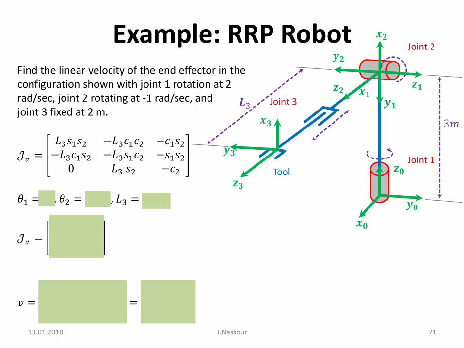
Find the linear velocity of the end effector in the configuration shown with joint 1 rotation at 2 rad/sec, joint 2 rotating at -1 rad/sec, and joint 3 fixed at 2 m.
Joint 3
Joint 1
Joint 2
Tool 𝒛𝟎
𝒙𝟎
𝒚𝟎
𝒛𝟏𝒙𝟏𝒚𝟏
𝒙𝟐
𝒚𝟐
𝒛𝟐
𝒛𝟑
𝒚𝟑
𝒙𝟑
𝑳3
3𝑚
J.Nassour 70
Example: RRP Robot
13.01.2018
Find the linear velocity of the end effector in the configuration shown with joint 1 rotation at 2 rad/sec, joint 2 rotating at -1 rad/sec, and joint 3 fixed at 2 m.
𝒥𝑣 =
𝐿3𝑠1𝑠2 −𝐿3𝑐1𝑐2 −𝑐1𝑠2−𝐿3𝑐1𝑠2 −𝐿3𝑠1𝑐2 −𝑠1𝑠2
0 𝐿3 𝑠2 −𝑐2
𝜃1 = 0°, 𝜃2 = −90°, 𝐿3 = 2 𝑚
𝒥𝑣 =0 0 12 0 00 −2 0
𝑣 =0 0 12 0 00 −2 0
2−10
=042
𝑚/𝑠
Joint 3
Joint 1
Joint 2
Tool 𝒛𝟎
𝒙𝟎
𝒚𝟎
𝒛𝟏𝒙𝟏𝒚𝟏
𝒙𝟐
𝒚𝟐
𝒛𝟐
𝒛𝟑
𝒚𝟑
𝒙𝟑
𝑳3
3𝑚
J.Nassour 71

Example: RRP Robot
13.01.2018
Find the linear velocity of the end effector in the configuration shown with joint 1 rotation at 2 rad/sec, joint 2 rotating at -1 rad/sec, and joint 3 fixed at 2 m.
𝒥𝑣 =
𝐿3𝑠1𝑠2 −𝐿3𝑐1𝑐2 −𝑐1𝑠2−𝐿3𝑐1𝑠2 −𝐿3𝑠1𝑐2 −𝑠1𝑠2
0 𝐿3 𝑠2 −𝑐2
𝜃1 = 0°, 𝜃2 = −90°, 𝐿3 = 2 𝑚
𝒥𝑣 =0 0 12 0 00 −2 0
𝑣 =0 0 12 0 00 −2 0
2−10
=042
𝑚/𝑠
Joint 3
Joint 1
Joint 2
Tool 𝒛𝟎
𝒙𝟎
𝒚𝟎
𝒛𝟏𝒙𝟏𝒚𝟏
𝒙𝟐
𝒚𝟐
𝒛𝟐
𝒛𝟑
𝒚𝟑
𝒙𝟑
𝑳3
3𝑚
J.Nassour 72

13.01.2018 J.Nassour 73
Inverting The Jacobian
• Analytical inverse (more DOF more Complexity)
• Numerical inverse

13.01.2018 J.Nassour 74
Reminder

Example: RRP Robot
13.01.2018
Find the joint velocities in the configuration shown if the desired linear velocities of the end effector are: 0 m/sec on x axis 4 m/sec on y axis 2 m/sec on z axis
𝒥𝑣 =
𝐿3𝑠1𝑠2 −𝐿3𝑐1𝑐2 −𝑐1𝑠2−𝐿3𝑐1𝑠2 −𝐿3𝑠1𝑐2 −𝑠1𝑠2
0 𝐿3 𝑠2 −𝑐2
𝜃1 = 0°, 𝜃2 = −90°, 𝐿3 = 2 𝑚
𝒥𝑣 =0 0 12 0 00 −2 0
𝒥𝑣−1 =
0 0.5 00 0 −0.51 0 0
Joint 3
Joint 1
Joint 2
Tool 𝒛𝟎
𝒙𝟎
𝒚𝟎
𝒛𝟏𝒙𝟏𝒚𝟏
𝒙𝟐
𝒚𝟐
𝒛𝟐
𝒛𝟑
𝒚𝟑
𝒙𝟑
𝑳3
3𝑚
J.Nassour 75

Example: RRP Robot
13.01.2018
Find the joint velocities in the configuration shown if the desired linear velocities of the end effector are: 0 m/sec on x axis 4 m/sec on y axis 2 m/sec on z axis
𝒥𝑣−1 =
0 0.5 00 0 −0.51 0 0
𝑞 =0 0.5 00 0 −0.51 0 0
042
=2−10
Joint 3
Joint 1
Joint 2
Tool 𝒛𝟎
𝒙𝟎
𝒚𝟎
𝒛𝟏𝒙𝟏𝒚𝟏
𝒙𝟐
𝒚𝟐
𝒛𝟐
𝒛𝟑
𝒚𝟑
𝒙𝟑
𝑳3
3𝑚
J.Nassour 76

Example: RRP Robot
13.01.2018
Find the joint velocities in the configuration shown if the desired linear velocities of the end effector are: 0 m/sec on x axis 4 m/sec on y axis 2 m/sec on z axis
𝒥𝑣−1 =
0 0.5 00 0 −0.51 0 0
𝑞 =0 0.5 00 0 −0.51 0 0
042
=2−10
Joint 3
Joint 1
Joint 2
Tool 𝒛𝟎
𝒙𝟎
𝒚𝟎
𝒛𝟏𝒙𝟏𝒚𝟏
𝒙𝟐
𝒚𝟐
𝒛𝟐
𝒛𝟑
𝒚𝟑
𝒙𝟑
𝑳3
3𝑚
J.Nassour 77

13.01.2018 J.Nassour 78
Example: NAO
Throwing in 2D only with ShoulderPitch and ElbowRoll.

13.01.2018 J.Nassour 79
Example: RR Robot
𝒙𝟎
𝒚𝟎
𝑰𝟏
𝑞1
𝑞2𝑰𝟐
Forward kinematics:
𝑋𝑒 = 𝐼1 𝑐1 + 𝐼2 𝑐12𝑌𝑒 = 𝐼1 𝑠1 + 𝐼2 𝑠12
End Effector
Xe
Ye
Find the end-effector velocities in function of joint velocities.
The total derivatives of the kinematics equations:
𝑑𝑋𝑒 =𝜕𝑋𝑒(𝑞1, 𝑞2)
𝜕𝑞1𝑑𝑞1+
𝜕𝑋𝑒(𝑞1, 𝑞2)
𝜕𝑞2𝑑𝑞2
𝑑𝑌𝑒 =𝜕𝑌𝑒(𝑞1, 𝑞2)
𝜕𝑞1𝑑𝑞1+
𝜕𝑌𝑒(𝑞1, 𝑞2)
𝜕𝑞2𝑑𝑞2
The Jacobian matrix represents the differential relationship between the joint displacement and the resulting end effector motion.
It comprises the partial derivatives of 𝑋𝑒(𝑞1, 𝑞2) and Y𝑒(𝑞1, 𝑞2)with respect to the joint displacements 𝑞1 and 𝑞2.

13.01.2018 J.Nassour 80
Example: RR Robot
𝒙𝟎
𝒚𝟎
𝑰𝟏
𝑞1
𝑞2𝑰𝟐
Forward kinematics:
𝑋𝑒 = 𝐼1 𝑐1 + 𝐼2 𝑐12𝑌𝑒 = 𝐼1 𝑠1 + 𝐼2 𝑠12
End Effector
Xe
Ye
𝒥𝑣 =
𝜕𝑋𝑒(𝑞1,𝑞2)
𝜕𝑞1
𝜕𝑋𝑒(𝑞1,𝑞2)
𝜕𝑞2𝜕𝑌
𝑒(𝑞
1,𝑞
2)
𝜕𝑞1
𝜕𝑌𝑒(𝑞
1,𝑞
2)
𝜕𝑞2
𝒥𝑣 = −𝐼1𝑠1− 𝐼2𝑠12 −𝐼2𝑠12𝐼1𝑐1 + 𝐼2𝑐12 𝐼2𝑐12

13.01.2018 J.Nassour 81
Example: RR Robot
𝒙𝟎
𝒚𝟎
𝑰𝟏
𝑞1
𝑞2𝑰𝟐
Forward kinematics:
𝑋𝑒 = 𝐼1 𝑐1 + 𝐼2 𝑐12𝑌𝑒 = 𝐼1 𝑠1 + 𝐼2 𝑠12
End Effector
Xe
Ye
𝒥𝑣 =
𝜕𝑋𝑒(𝑞1,𝑞2)
𝜕𝑞1
𝜕𝑋𝑒(𝑞1,𝑞2)
𝜕𝑞2𝜕𝑌
𝑒(𝑞
1,𝑞
2)
𝜕𝑞1
𝜕𝑌𝑒(𝑞
1,𝑞
2)
𝜕𝑞2
𝒥𝑣 = −𝐼1𝑠1− 𝐼2𝑠12 −𝐼2𝑠12𝐼1𝑐1 + 𝐼2𝑐12 𝐼2𝑐12

13.01.2018 J.Nassour 82
Example: RR Robot
𝒙𝟎
𝒚𝟎
𝑰𝟏
𝑞1
𝑞2𝑰𝟐
Forward kinematics:
𝑋𝑒 = 𝐼1 𝑐1 + 𝐼2 𝑐12𝑌𝑒 = 𝐼1 𝑠1 + 𝐼2 𝑠12
End Effector
Xe
Ye
𝒥𝑣 = −𝐼1𝑠1− 𝐼2𝑠12 −𝐼2𝑠12𝐼1𝑐1 + 𝐼2𝑐12 𝐼2𝑐12
We can divide the 2-by-2 Jacobian into two column vectors:
𝒥𝑣= (𝒥1 , 𝒥2), 𝒥1 , 𝒥2 ∈ 𝕽2 × 1
We can then write the resulting end-effector velocity vector:
𝑉𝑒 = 𝒥1 . 𝑞1+ 𝒥2 . 𝑞2
Each column vector of the Jacobian matrix represents the end –effector velocity generated by the corresponding joint moving when all other joints are not moving.

13.01.2018 J.Nassour 83
Example: RR Robot
𝒙𝟎
𝒚𝟎
𝑰𝟏
𝑞1
𝑞2𝑰𝟐
Forward kinematics:
𝑋𝑒 = 𝐼1 𝑐1 + 𝐼2 𝑐12𝑌𝑒 = 𝐼1 𝑠1 + 𝐼2 𝑠12
End Effector
Xe
Ye
𝒥𝑣 = −𝐼1𝑠1− 𝐼2𝑠12 −𝐼2𝑠12𝐼1𝑐1 + 𝐼2𝑐12 𝐼2𝑐12
𝒥1 =−𝐼1𝑠1 − 𝐼2𝑠12𝐼1𝑐1+ 𝐼2𝑐12
𝒥2 =−𝐼2𝑠12𝐼2𝑐12

13.01.2018 J.Nassour 84
Example: RR Robot
𝒙𝟎
𝒚𝟎
𝑰𝟏
𝑞1
𝑞2𝑰𝟐
Forward kinematics:
𝑋𝑒 = 𝐼1 𝑐1 + 𝐼2 𝑐12𝑌𝑒 = 𝐼1 𝑠1 + 𝐼2 𝑠12
End Effector
𝒥1 =−𝐼1𝑠1 − 𝐼2𝑠12𝐼1𝑐1 + 𝐼2𝑐12
, 𝒥2 =−𝐼2𝑠12𝐼2𝑐12
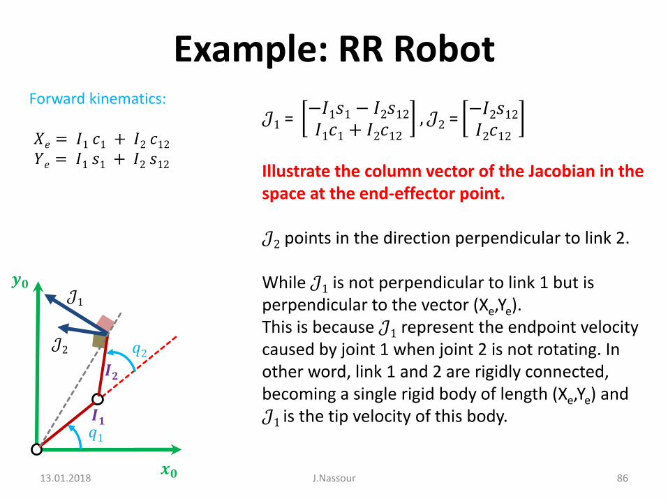
Illustrate the column vector of the Jacobian in the space at the end-effector point.

13.01.2018 J.Nassour 85
Example: RR Robot
𝒙𝟎
𝒚𝟎
𝑰𝟏
𝑞1
𝑞2𝑰𝟐
Forward kinematics:
𝑋𝑒 = 𝐼1 𝑐1 + 𝐼2 𝑐12𝑌𝑒 = 𝐼1 𝑠1 + 𝐼2 𝑠12
End Effector
𝒥1 =−𝐼1𝑠1 − 𝐼2𝑠12𝐼1𝑐1 + 𝐼2𝑐12
, 𝒥2 =−𝐼2𝑠12𝐼2𝑐12
Illustrate the column vector of the Jacobian in the space at the end-effector point.
𝒥2 points in the direction perpendicular to link 2.
While 𝒥1 is not perpendicular to link 1 but is perpendicular to the vector (Xe,Ye).This is because 𝒥1 represent the endpoint velocity caused by joint 1 when joint 2 is not rotating.In other word, link 1 and 2 are rigidly connected, becoming a single rigid body of length (Xe,Ye) and 𝒥1 is the tip velocity of this body.
13.01.2018 J.Nassour 86
Example: RR Robot
𝒙𝟎
𝒚𝟎
𝑰𝟏𝑞1
𝑞2𝑰𝟐
Forward kinematics:
𝑋𝑒 = 𝐼1 𝑐1 + 𝐼2 𝑐12𝑌𝑒 = 𝐼1 𝑠1 + 𝐼2 𝑠12
𝒥1 =−𝐼1𝑠1 − 𝐼2𝑠12𝐼1𝑐1 + 𝐼2𝑐12
, 𝒥2 =−𝐼2𝑠12𝐼2𝑐12
Illustrate the column vector of the Jacobian in the space at the end-effector point.
𝒥2 points in the direction perpendicular to link 2.
While 𝒥1 is not perpendicular to link 1 but is perpendicular to the vector (Xe,Ye).This is because 𝒥1 represent the endpoint velocity caused by joint 1 when joint 2 is not rotating. In other word, link 1 and 2 are rigidly connected, becoming a single rigid body of length (Xe,Ye) and 𝒥1 is the tip velocity of this body.
𝒥2
𝒥1

13.01.2018 J.Nassour 87
Example: RR Robot
𝒙𝟎
𝒚𝟎
𝑰𝟏𝑞1
𝑞2𝑰𝟐
Forward kinematics:
𝑋𝑒 = 𝐼1 𝑐1 + 𝐼2 𝑐12𝑌𝑒 = 𝐼1 𝑠1 + 𝐼2 𝑠12
𝒥1 =−𝐼1𝑠1 − 𝐼2𝑠12𝐼1𝑐1 + 𝐼2𝑐12
, 𝒥2 =−𝐼2𝑠12𝐼2𝑐12
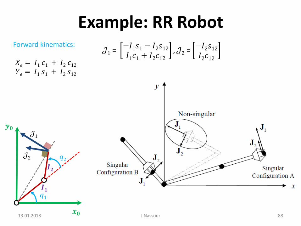
If the two Jacobian column vectors are aligned, the end-effector can not be moved in an arbitrary direction.
This may happen for particular arm configurations when the two links are fully contracted or extracted.
These arm configurations are referred to as singular configurations.
ACCORDINGLY, the Jacobian matrix become singular at these positions.
Find out the singular configurations…
𝒥2
𝒥1
13.01.2018 J.Nassour 88
Example: RR Robot
𝒙𝟎
𝒚𝟎
𝑰𝟏𝑞1
𝑞2𝑰𝟐
Forward kinematics:
𝑋𝑒 = 𝐼1 𝑐1 + 𝐼2 𝑐12𝑌𝑒 = 𝐼1 𝑠1 + 𝐼2 𝑠12
𝒥1 =−𝐼1𝑠1 − 𝐼2𝑠12𝐼1𝑐1 + 𝐼2𝑐12
, 𝒥2 =−𝐼2𝑠12𝐼2𝑐12
𝒥2
𝒥1

13.01.2018 J.Nassour 89
Example: RR Robot
𝒙𝟎
𝒚𝟎
𝑰𝟏𝑞1
𝑞2𝑰𝟐
Forward kinematics:
𝑋𝑒 = 𝐼1 𝑐1 + 𝐼2 𝑐12𝑌𝑒 = 𝐼1 𝑠1 + 𝐼2 𝑠12
𝒥𝑣 = −𝐼1𝑠1 − 𝐼2𝑠12 −𝐼2𝑠12𝐼1𝑐1 + 𝐼2𝑐12 𝐼2𝑐12
The Jacobian reflects the singular configurations.When joint 2 is 0 or 180 degrees:
𝑑𝑒𝑡 𝒥𝑣 = det− 𝐼1 ± 𝐼2 𝑠1 ∓𝐼2𝑠1𝐼1 ± 𝐼2 𝑐1 ±𝐼2𝑐1
= 0
𝒥2
𝒥1

13.01.2018 J.Nassour 90
Example: RR Robot
𝒙𝟎
𝒚𝟎
𝑰𝟏𝑞1
𝑞2𝑰𝟐
Forward kinematics:
𝑋𝑒 = 𝐼1 𝑐1 + 𝐼2 𝑐12𝑌𝑒 = 𝐼1 𝑠1 + 𝐼2 𝑠12
𝒥𝑣 = −𝐼1𝑠1 − 𝐼2𝑠12 −𝐼2𝑠12𝐼1𝑐1 + 𝐼2𝑐12 𝐼2𝑐12
The Jacobian reflects the singular configurations.When joint 2 is 0 or 180 degrees:
𝑑𝑒𝑡 𝒥𝑣 = det− 𝐼1 ± 𝐼2 𝑠1 ∓𝐼2𝑠1𝐼1 ± 𝐼2 𝑐1 ±𝐼2𝑐1
= 0
𝒥2
𝒥1

13.01.2018 J.Nassour 91
Example: RR Robot
𝒙𝟎
𝒚𝟎
𝑰𝟏𝑞1
𝑞2𝑰𝟐
𝒥2
𝒥1
Work out the joint velocities 𝒒 ( 𝒒𝟏, 𝒒𝟐) in terms of the end effector velocity Ve(Vx,Vy).
If the arm configuration is not singular, this can be obtained by taking the inverse of the Jacobian matrix:
𝑞 = 𝐽−1. 𝑉𝑒
Note that the differential kinematics problem has a unique solution as long as the Jacobian is non-singular.
Since the elements of the Jacobian matrix are function of joint displacements, the inverse Jacobian varies depending on the arm configuration. This means that although the desired end-effector velocity is constant, the joint velocities are not.

13.01.2018 J.Nassour 92
Example: RR Robot
𝒙𝟎
𝒚𝟎
𝑰𝟏𝑞1
𝑞2𝑰𝟐
𝒥2
𝒥1
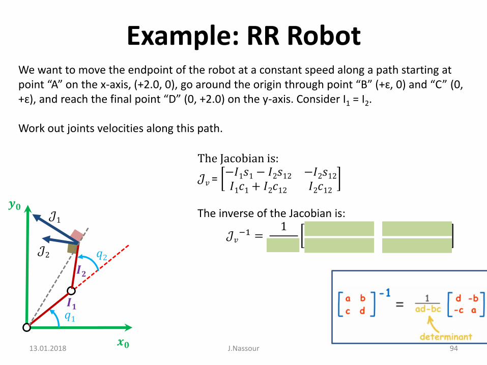
We want to move the endpoint of the robot at a constant speed along a path starting at point “A” on the x-axis, (+2.0, 0), go around the origin through point “B” (+ɛ, 0) and “C” (0, +ɛ), and reach the final point “D” (0, +2.0) on the y-axis. Consider I1 = I2.
Work out joints velocities along this path.
D

13.01.2018 J.Nassour 93
Example: RR Robot
𝒙𝟎
𝒚𝟎
𝑰𝟏𝑞1
𝑞2𝑰𝟐
𝒥2
𝒥1
We want to move the endpoint of the robot at a constant speed along a path starting at point “A” on the x-axis, (+2.0, 0), go around the origin through point “B” (+ɛ, 0) and “C” (0, +ɛ), and reach the final point “D” (0, +2.0) on the y-axis. Consider I1 = I2.
Work out joints velocities along this path.
The Jacobian is:
𝒥𝑣 = −𝐼1𝑠1 − 𝐼2𝑠12 −𝐼2𝑠12𝐼1𝑐1+ 𝐼2𝑐12 𝐼2𝑐12
13.01.2018 J.Nassour 94
Example: RR Robot
𝒙𝟎
𝒚𝟎
𝑰𝟏𝑞1
𝑞2𝑰𝟐
𝒥2
𝒥1
The Jacobian is:
𝒥𝑣 = −𝐼1𝑠1 − 𝐼2𝑠12 −𝐼2𝑠12𝐼1𝑐1+ 𝐼2𝑐12 𝐼2𝑐12
The inverse of the Jacobian is:
𝒥𝑣−1 =
1
𝐼1𝐼2𝑠2
𝐼2𝑐12 𝐼2𝑠12−𝐼1𝑐1− 𝐼2𝑐12 −𝐼1𝑠1 − 𝐼2𝑠12
We want to move the endpoint of the robot at a constant speed along a path starting at point “A” on the x-axis, (+2.0, 0), go around the origin through point “B” (+ɛ, 0) and “C” (0, +ɛ), and reach the final point “D” (0, +2.0) on the y-axis. Consider I1 = I2.
Work out joints velocities along this path.

13.01.2018 J.Nassour 95
Example: RR Robot
𝒙𝟎
𝒚𝟎
𝑰𝟏𝑞1
𝑞2𝑰𝟐
𝒥2
𝒥1
The inverse of the Jacobian is:
𝒥𝑣−1 =
1
𝐼1𝐼2𝑠2
𝐼2𝑐12 𝐼2𝑠12−𝐼1𝑐1− 𝐼2𝑐12 −𝐼1𝑠1 − 𝐼2𝑠12
𝑞1 =𝐼2𝑐12. 𝑉𝑥 + 𝐼2𝑠12. 𝑉𝑦
𝐼1𝐼2𝑠2
𝑞2 =−𝐼1𝑐1− 𝐼2𝑐12 . 𝑉𝑥 + [−𝐼1𝑠1− 𝐼2𝑠12]. 𝑉𝑦
𝐼1𝐼2𝑠2
We want to move the endpoint of the robot at a constant speed along a path starting at point “A” on the x-axis, (+2.0, 0), go around the origin through point “B” (+ɛ, 0) and “C” (0, +ɛ), and reach the final point “D” (0, +2.0) on the y-axis. Consider I1 = I2.
Work out joints velocities along this path.

13.01.2018 J.Nassour 96
𝑞1 =𝐼2𝑐12. 𝑉𝑥 + 𝐼2𝑠12. 𝑉𝑦
𝐼1𝐼2𝑠2
𝑞2 =−𝐼1𝑐1 − 𝐼2𝑐12 . 𝑉𝑥 + [−𝐼1𝑠1 − 𝐼2𝑠12]. 𝑉𝑦
𝐼1𝐼2𝑠2
D

13.01.2018 J.Nassour 97
𝑞1 =𝐼2𝑐12. 𝑉𝑥 + 𝐼2𝑠12. 𝑉𝑦
𝐼1𝐼2𝑠2
𝑞2 =−𝐼1𝑐1 − 𝐼2𝑐12 . 𝑉𝑥 + [−𝐼1𝑠1 − 𝐼2𝑠12]. 𝑉𝑦
𝐼1𝐼2𝑠2
D

13.01.2018 J.Nassour 98
Example: RR Robot
Note that the joint velocities are extremely large near the initial and the final points, and are unbounded at points A and D. These are the arm singular configurations q2=0.
𝑞1 =𝐼2𝑐12. 𝑉𝑥 + 𝐼2𝑠12. 𝑉𝑦
𝐼1𝐼2𝑠2
𝑞2 =−𝐼1𝑐1− 𝐼2𝑐12 . 𝑉𝑥 + [−𝐼1𝑠1− 𝐼2𝑠12]. 𝑉𝑦
𝐼1𝐼2𝑠2
D

13.01.2018 J.Nassour 99
Example: RR Robot
𝑞1 =𝐼2𝑐12. 𝑉𝑥 + 𝐼2𝑠12. 𝑉𝑦
𝐼1𝐼2𝑠2
𝑞2 =−𝐼1𝑐1− 𝐼2𝑐12 . 𝑉𝑥 + [−𝐼1𝑠1− 𝐼2𝑠12]. 𝑉𝑦
𝐼1𝐼2𝑠2
As the end-effector gets close to the origin, the velocity of the first joint becomes very large in order to quickly turn the arm around from point B to C. At these configurations, the second joint is almost -180 degrees, meaning that the arm is near singularity.
D

13.01.2018 J.Nassour 100
Example: RR Robot
𝑞1 =𝐼2𝑐12. 𝑉𝑥 + 𝐼2𝑠12. 𝑉𝑦
𝐼1𝐼2𝑠2
𝑞2 =−𝐼1𝑐1− 𝐼2𝑐12 . 𝑉𝑥 + [−𝐼1𝑠1− 𝐼2𝑠12]. 𝑉𝑦
𝐼1𝐼2𝑠2
This result agrees with the singularity condition using the determinant of the Jacobian:
𝑑𝑒𝑡 𝒥𝑣 = sin 𝑞2 = 0 for 𝑞2 = 𝑘𝜋, 𝑘 = 0, ±1,±2,…
D

13.01.2018 J.Nassour 101
Example: RR Robot
𝒙𝟎
𝒚𝟎
𝑰𝟏𝑞1
𝑞2𝑰𝟐
𝒥2
𝒥1
Using the Jacobian, analyse the arm behaviour at the singular points. Consider (l1=l2=1).
The Jacobian is:
𝒥𝑣 = −𝐼1𝑠1 − 𝐼2𝑠12 −𝐼2𝑠12𝐼1𝑐1+ 𝐼2𝑐12 𝐼2𝑐12
, 𝒥1 =−𝐼1𝑠1− 𝐼2𝑠12𝐼1𝑐1+ 𝐼2𝑐12
, 𝒥2 =−𝐼2𝑠12𝐼2𝑐12
For q2=0:
𝒥1 =−2𝑠12𝑐1
, 𝒥2 =−𝑠1𝑐1
The Jacobian column vectors reduce to the ones in the same direction. Note that no endpoint velocity can be generated in the direction perpendicular to the aligned arm links (singular configuration A and D).

13.01.2018 J.Nassour 102
Example: RR Robot
𝒙𝟎
𝒚𝟎
𝑰𝟏𝑞1
𝑞2𝑰𝟐
𝒥2
𝒥1
Using the Jacobian, analyse the arm behaviour at the singular points. Consider (l1=l2=1).
The Jacobian is:
𝒥𝑣 = −𝐼1𝑠1 − 𝐼2𝑠12 −𝐼2𝑠12𝐼1𝑐1+ 𝐼2𝑐12 𝐼2𝑐12
, 𝒥1 =−𝐼1𝑠1− 𝐼2𝑠12𝐼1𝑐1+ 𝐼2𝑐12
, 𝒥2 =−𝐼2𝑠12𝐼2𝑐12
For q2=𝝅:
𝒥1 =00, 𝒥2 =
𝑠1−𝑐1
The first joint cannot generate any endpoint velocity, since the arm is fully contracted (singular configuration B).

13.01.2018 J.Nassour 103
Example: RR Robot
𝒙𝟎
𝒚𝟎
𝑰𝟏𝑞1
𝑞2𝑰𝟐
𝒥2
𝒥1
Using the Jacobian, analyse the arm behaviour at the singular points. Consider (l1=l2=1).
At the singular configuration, there is at least one direction is which the robot cannot generate a non-zero velocity at the end effector.

Example: RRR Robot
13.01.2018
The robot has three revolute joints that allow the endpoint to move in the three dimensional space. However, this robot mechanism has singular points inside the workspace. Analyze the singularity, following the procedure below.
J.Nassour 104
Link 0 (fixed)
Joint 1
Link 1
Joint variable 𝜽1
Joint 2
Link 2
Joint variable 𝜽2
Link 3
𝒛𝟐
Joint 3
Joint variable 𝜽3
𝒛𝟑
𝒙𝟎
𝒚𝟎
𝒛𝟎
𝒛𝟏 𝒙𝟏
𝒚𝟏
𝒙𝟐
𝒚𝟐
𝒙𝟑
𝒚𝟑
Link 1= 2 mLink 2= 2 mLink 3= 2 m
Step 3 Find the joint angles that make det J =0.Step 4 Show the arm posture that is singular. Show where in the workspace it becomes singular. For each singular configuration, also show in which direction the endpoint cannot have a non-zero velocity.
Step 1 Obtain each column vector of the Jacobian matrix by considering the endpoint velocity created by each of the joints while immobilizing the other joints.
Step 2 Construct the Jacobian by concatenating the column vectors, and set the determinant of the Jacobian to zero for singularity: det J =0.

13.01.2018 J.Nassour 105
Stanford Arm
𝒅𝟑
𝑑6
𝜽𝟏
𝜽𝟐
𝜽𝟒
𝜽𝟓
𝜽𝟔
𝒛𝟎
𝒛𝟏
𝒛𝟐
𝒛𝟒
𝒛𝟑 𝒛𝟓
𝑑2
𝒛𝟔
𝒙𝟏 𝒙𝟐
𝒙
𝒚𝟔
𝒙𝟔
Give one example of singularity that can occur.
Whenever 𝜽𝟓 = 𝟎 , the manipulator is in a singular configuration because joint 4 and 6 line up. Both joints actions would results the same end-effector motion (one DOF will be lost).

13.01.2018 J.Nassour 106
PUMA 260
𝜽𝟏
𝜽𝟐
𝜽𝟑
𝜽𝟒
𝜽𝟓 𝜽𝟔
𝒛𝟎
𝒙𝟎𝒚𝟎
𝒙𝟏
𝒛𝟏
𝒚𝟏
𝒙𝟐
𝒛𝟐
𝒚𝟐𝒙𝟑
𝒚𝟑
𝒛𝟑
𝒛𝟒𝒚𝟒
𝒙𝟒
𝒙𝟓
𝒚𝟓𝒛𝟓
𝒙𝟔
𝒚𝟔𝒛𝟔
𝒅𝟐
𝒂𝟐
𝒅𝟒
𝒂𝟑
𝒅𝟔
Give two examples of singularities that can occur.
Whenever 𝜽𝟓 = 𝟎 , the manipulator is in a singular configuration because joint 4 and 6 line up. Both joints actions would results the same end-effector motion (one DOF will be lost).
Whenever 𝜽𝟑 = −𝟗𝟎 , the manipulator is in a singular configuration. In this situation, the arm is fully extracted. This is classed as a workspace boundary singularity.

13.01.2018 J.Nassour 107
𝜽𝟏
𝜽𝟐
𝜽𝟑
𝜽𝟒
𝜽𝟓
𝒛𝑻
𝒙𝑻𝒚𝑻
𝒛𝟎𝒙𝟎
𝒚𝟎
𝒛𝟏
𝒚𝟏𝒙𝟏
𝒛𝟐
𝒚𝟐
𝒙𝟐
𝒚𝟑
𝒙𝟑
𝒛𝟑
𝒛𝟒
𝒙𝟒
𝒚𝟒
NAO Left Arm
𝒛𝟓
𝒙𝟓𝒚𝟓

13.01.2018 J.Nassour 108
NAO Right Arm