International Journal of Dynamics of Fluids ISSN 0973-1784 Volume 5, Number 1 (2009), pp. 61–83 © Research India Publications http://www.ripublication.com/ijdf.htm

Velocity Profiles and Wall Shear Stress in Turbulent

Transient Pipe Flow

H. Zidouh

Laboratoire de Mécanique et Énergétique

Université de Valenciennes, Valenciennes 59313, France Email: hamid.zidouh@gmail.com

Abstract

Experimental measurements of the wall shear stress combined to those of the velocity profiles via the electrochemical technique and ultrasonic pulsed Doppler velocimetry, are used to analyse the flow behaviour in transient pipe flow caused by a downstream sudden valve closure. Velocity data are analyzed and the corresponding wall shear stress values are evaluated, leading to a discussion on transient energy dissipation by comparison with results obtained by the electrochemical technique. The Reynolds number of the steady flow based on the pipe diameter is Re=140000 . The results show that the quasi-steady approach of representing unsteady friction is valid during the initial phase for relatively large decelerations. For higher decelerations, the unsteady wall shear stress is consistently higher than the quasi-steady values obtained from the velocity profiles. An examination of the range of applicability of the instantaneous-acceleration model shows that the empirical coefficient of unsteady friction is closely linked to the deceleration intensity. This study is made possible owing to the repeatability of different valve closures allowing data to be averaged over numerous tests.

Introduction Transient flows associated with the water hammer phenomenon are commonly encountered in both natural and engineering systems, such hydraulic and pneumatic control system, oil transportation system and human arterial network. Sudden changes in pressurized pipe flow conditions caused by pump starts and stops, valve operation, are routine events. The dramatic changes in velocity and pressure arising from these transient events can cause pipe breaks, flooding and other damage hazards.

Historically, it is assumed that phenomenological expressions that relate wall shear stress to cross sectional averaged velocity in steady state flows remain valid

62 H. Zidouh

under unsteady conditions. That is, wall shear expressions, such as the Darcy-Weisbach formula (Eq. 1), are assumed to hold at every instant during a transient:

( ) ( ) ( ) ( ) / 8w wst t f U t U tτ τ ρ≈ = (1)

Where f is the Darcy-Weisbach friction factor and wsτ is quasi-steady wall shear

stress as a function of t . In other words, the quasi-steady approach assumes the friction factor, hence the

wall shear stress, to be dependent on the local and actual Reynolds number. The application of such a simplified friction model is satisfactory only for very slow transients, in which the shape of the instantaneous velocity profiles does not differ markedly from the corresponding steady-state ones. During fast transients (rapidly changing flows) or high frequency periodic flows, on the other hand, velocity profiles change in particular and more complex manners (Brunone et al. [1] and Zidouh et al. [2]) showing greater gradients, hence greater shear stress, than the corresponding steady flow values. During these fast transients, the quasi-steady approach is not valid, as underestimates the friction forces and overestimates the persistence of oscillations following the first one, leading to discrepancies between numerical results and experimental data (Eichinger and Lein [3], Brunone et al. [1], Bergant et al. [4]).

The traditional approach is to introduce mathematically such a discrepancy as

( )wu tτ = difference between the instantaneous wall shear stress ( )w tτ and the quasi-

steady wall shear stress ( )ws tτ :

( ) ( ) ( )w ws wut t tτ τ τ= + (2)

Where wuτ is zero for steady flows, small for slow transients and significant for

fast transients. The unsteady friction terms can be classified into six groups (Bergant et al. [4]):

(1) The friction term is dependent on instantaneous mean flow velocity U , (Cocchi [5]; Hino et al. [6]);

(2) The friction term is dependent on instantaneous mean flow velocity U and instantaneous local acceleration /U t∂ ∂ , (Daily et al. [7], Cartsens and Roller [8], Shuy [9] and Safwat and Van der Polder [10]);

(3) The friction term is dependent on instantaneous mean flow velocity U and instantaneous local acceleration /U t∂ ∂ , and instantaneous convective acceleration /U x∂ ∂ , (Brunone et al. [11]);

(4) The friction term is dependent on instantaneous mean flow velocity U and diffusion 2 2/U x∂ ∂ (Vennatrø, [12], Svingen [13]);

(5) The friction term is dependent on instantaneous mean flow velocity U and weights for velocity changes ( )W τ (Zielke [14], Trikha [15], Vardy et al.

[16] and Vardy and Brown [17-20]);

Velocity Profiles and Wall Shear Stress 63

(6) The friction term is based on cross-sectional distribution of instantaneous flow velocity (Eichinger and Lein [3]; Vardy and Hwang [21], Silva-Araya and Chaudhry [22], Pezzinga [23]).

Daily et al. [7] conducted laboratory experiments and found ( )wu tτ to be positive

for accelerating flows and negative for decelerating flows. They argued that during acceleration, the central portion of the stream moved somewhat bodily so that the velocity profile steepened, giving higher shear. The relation postulated by Daily et al. [7] can be rewritten as:

8w ws

k D U

t

ρτ τ ∂= +∂

(3)

where k , the unsteady friction factor, needs to be determined either from experiment or analysis.

The theoretical work of Cartsens and Roller [8] shows only that Eq. 3 applies to very slow transients in which the unsteady velocity profile has the same shape as the steady velocity profile. Shuy [9] rewrites Eq. 3 in the form:

2u s

kD dUf f

U dt= + (4)

and defines an acceleration parameter, φ :

2

2

s

D dU

f U dtφ = (5)

Daily et al. [7] showed that 0.01k = for accelerating flows and 0.62k = for

decelerating flows. On the other hand, the research of Shuy [9] led to 0.0825k = − for accelerating flows and 0.13k = − for decelerating flows. This illustrates that the unsteady friction factor is flow case dependent. To explain these conflicting results, Vardy and Brown [24], argue that the different behaviours observed by the authors may be attributed to different time-scales. Brunone and Golia [25], Greco [26], and Brunone et al. [11, 17] have provided a very important modification to unsteady friction models based on instantaneous acceleration. The Brunone et al. [11] model

relates unsteady friction part uτ to the instantaneous local acceleration and

instantaneous convective acceleration /U x∂ ∂ : The data of Brunone et al. [1], Daily et al. [7], and others show that k is not a

universal constant. Vardy and Brown [18] proposed the following empirical relationship to derive this coefficient analytically:

* / 2k C= (6)

where *C is the Vardy’s shear decay coefficient.

64 H. Zidouh

Zielke [14] derived weighting function model for laminar transient flows, beginning from the Navier-Stokes equations. This model relates the wall shear stress to the instantaneous mean velocity and the weighted past history changes. The Zielke [14] model requires large computer storage and has been modified by several researchers to improve the computational efficiency and/or to extend its application to the turbulent transient flow conditions (Trikha [15], Vardy et al. [16], Vardy and Brown [17, 18], and Schohl [28]).

The measurements of the unsteady wall shear stress so far were conducted in previous studies by measuring the wall drag force (Shuy [9]) or by determining the transient friction coefficient from the instantaneous mean flow velocity (Kurokawa and Morikawa [29]). Whereas the above mentioned approaches are acceptable for flows accelerating or deceleration slowly at a uniform rate, they are questionable during fast transients. Moreover, the studies so far performed about transient flows are limited to very narrow ranges of accelerations and deceleration, and the results obtained by these studies are very different from one another.

Specifically, it was noted that accelerated or decelerated phases, during a water hammer transient, behave in a different manner depending on the timescale investigated. The analysis has shown a strong influence of the history of the transient on the energy dissipation mechanism. In particular, during decelerations, it was noted that, for short time scales, i.e. at the beginning of the transient, when the effect of single pressure waves is clearly detectable, the observed wall shear stress is lower than the corresponding pseudo-steady state one. On the other hand, long timescales are characterized by increasing wall shear stress values that soon become higher than corresponding pseudo-steady ones, leading to a higher energy dissipation also during decelerated phases. On the other hand, during accelerations, it was noted that, for short timescales, a different trend occurs depending on pipe section, hence on velocity profile evolution.

From this brief review, it is shown that a critical lack of experimental data for characterizing turbulent transient flow. This lack of knowledge does not allow a precise determination of the local unsteady wall shear. It is shown that no conclusive result was attained because of the little experimental data available. A non-intrusive, local and quantitative method is actually greatly required to determine the important unsteady phenomena involved under transient conditions. The primary aim of this work was to determine the local wall shear stress in turbulent transient flow. This is made possible by the use of the electrochemical method.

Experimental approach The electrochemical technique is one of the non-intrusive methods used for the measurement of the local wall shear rate (Hanratty and Campbell [30]). The principle of this technique has been widely described in past by Reiss and Hanratty [31], Lebouché [32] and Cognet [33]. The principle of this method consists of measuring the limiting diffusion current at the cathode of an electrolysis cell during an electrochemical reaction, so as to determine the mass transfer rate. This under conditions diffusion-controlled conditions for which this reaction is high enough to

Velocity Profiles and Wall Shear Stress 65

consider that the concentration of the reacting ions is zero at the surface of the working electrode. Under diffusion-controlled conditions, the mass transfer coefficient, K , between the electrolyte and the probe surface is related to limiting diffusion current, I , by:

0/K I n AC= F (7)

where n is the number of electrons involved in the reaction, F is Faraday’s

constant, A is the active surface of the electrochemical probe, and 0C is the bulk

concentration of the active ions. The relationship between the wall shear stress and the electrolysis current is given

in dimensionless form by Son and Hanratty [34] and by Lebouché [32]:

1/3K bS+ += (8) with /K Kl+ = D and 0/K I n AC= F for single probe

1 2

1 2

K KK

K K+ −=

+ for double probe in differential mode

2 /S Sl+ = D and / /S u yτ μ= = ∂ ∂ where Δ is the diffusivity.

The integration of the mass transfer equation, by Son and Hanratty [34] and by

Lebouché [32], gives a theoretical value for the coefficient b : simple rectangular probe, 0.807b = ; double rectangular probe in differential mode, 0.21b = . In the case of a circular probe with diameter d , Py and Gosse [35] and Reiss and Hanratty [31] demonstrated that Eq. 8 is still valid with 0.82l d= .

For quasi-steady regime, the Levêque [36] solution can only be used for high Peclet numbers and the one-third power law (Eq. 8) can be used to calculate the instantaneous wall shear rate (Hanratty and Campbell [30]). For high frequency fluctuating flow, the Levêque solution cannot predict the real wall shear rate, an attenuation of the signal fluctuation and a phase shift are observed. These discrepancies are caused by the capacitive effect of the concentration boundary layer, which is acting as a low-pass filter (Rehimi et al. [37]).

The most common approaches related to the wall shear stress probes are focused on the research of transfer functions between wall shear stress and limiting diffusion current (Mitchell and Hanratty [38]; Deslouis et al. [39] and Maquinghen [40]). In these works, the axial diffusion mass transfer was neglected and they are generally based on a linearization of the problem by assuming that the wall shear rate fluctuations remain small in comparison with the average value. This approach is not always valid. For example, in flows involving large amplitude oscillations or reversing flows, the above mentioned approach cannot apply.

The direct correction of the electrochemical signals seems to be quite an attractive method to solve the dynamic behaviour of the electrochemical probes. Sobolik et al. [41] have introduced a technique based on the correction of the wall shear rate

66 H. Zidouh

obtained by the Levêque solution by adding a term deduced from the transient response of a probe multiplied by the time derivative of mass transfer rate. The approximate solution may be expressed as follows:

( ) ( ) ( )0

2

3qs

c qs

S tS t S t t

t

∂= +

∂ (9)

where the first term on the right-hand side of Eq. 9 corresponds to the quasi-

steady solution and the second term represents the inertial effect. In the present study, the characteristic time of the probe, 0t , was obtained experimentally by using the

Cotrell method (Wein [42]; Tihon et al. [43] and Sobolik et al. [44]). This technique is based on the study of the transient response of the probes to a voltage step from 0 to the diffusional plateau potential. This method is also used to determine the active surface of the electrochemical probes.

The inverse method, which does not require a linearization assumption, is more appropriate for calculating the velocity gradient at the wall from measured mass transfer signal. This method has been developed by Mao and Hanratty [45], based on a numerical solution similar to that reported by Kaiping [46], and later by Maquinghen [47]. This technique consists in solving the direct convection-diffusion equation and in estimating sequentially the unknown wall shear rate by minimizing the difference between measured and simulated mean concentration gradient on the probe surface.

In this study, both the inverse method and that suggested by Sobolik et al. [41] have been used to determinate the ’true’ wall shear rate from the measured limiting diffusion current.

Experimental apparatus Experimental installation Experiments were conducted at an experimental apparatus (Fig. 1) specially designed in order to investigate the waterhammer phenomenon. This experimental apparatus comprises a polypropylene pipe of length L=2.62 m, D=61.4 mm internal diameter and e=6.8 mm wall thickness. The pipe is connected to a supply and recycling system. The pipe is rigidly fixed in order to minimize its vibrations. An constant level tank is used to keep upstream pressures constant during measurements. Unsteady flow conditions are generated and regulated by a butterfly valve at the downstream end of the pipe. The experimental apparatus is fully described by Zidouh [47].

Pressure, velocity and wall shear stress are measured in section S1, 3.27 m downstream from the free surface. The test rig is equipped with appropriate measuring instrumentation. The transient pressure was measured using a transducers of the stainless diaphragm type which had a full range of 7 bar with 0.5 % accuracy. Recording of the pressure and the friction changes was carried out with a sampling frequency of 10 kHz using a computerized data acquisition system.

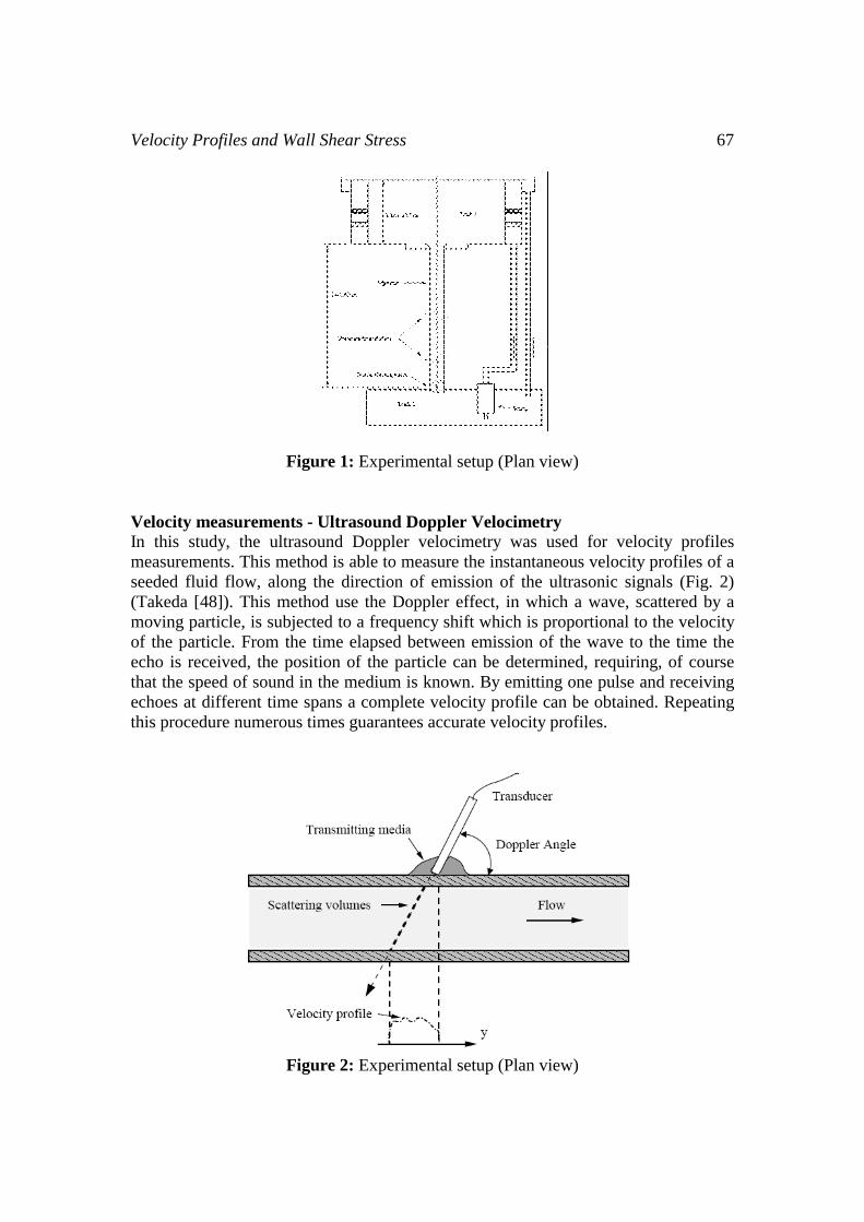
Velocity Profiles and Wall Shear Stress 67

Figure 1: Experimental setup (Plan view)

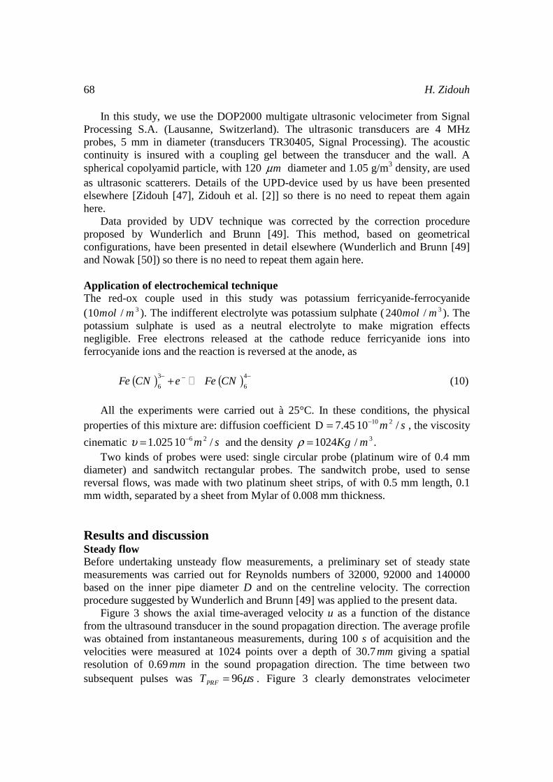
Velocity measurements - Ultrasound Doppler Velocimetry In this study, the ultrasound Doppler velocimetry was used for velocity profiles measurements. This method is able to measure the instantaneous velocity profiles of a seeded fluid flow, along the direction of emission of the ultrasonic signals (Fig. 2) (Takeda [48]). This method use the Doppler effect, in which a wave, scattered by a moving particle, is subjected to a frequency shift which is proportional to the velocity of the particle. From the time elapsed between emission of the wave to the time the echo is received, the position of the particle can be determined, requiring, of course that the speed of sound in the medium is known. By emitting one pulse and receiving echoes at different time spans a complete velocity profile can be obtained. Repeating this procedure numerous times guarantees accurate velocity profiles.

Figure 2: Experimental setup (Plan view)

68 H. Zidouh

In this study, we use the DOP2000 multigate ultrasonic velocimeter from Signal Processing S.A. (Lausanne, Switzerland). The ultrasonic transducers are 4 MHz probes, 5 mm in diameter (transducers TR30405, Signal Processing). The acoustic continuity is insured with a coupling gel between the transducer and the wall. A spherical copolyamid particle, with 120 mμ diameter and 1.05 g/m3 density, are used as ultrasonic scatterers. Details of the UPD-device used by us have been presented elsewhere [Zidouh [47], Zidouh et al. [2]] so there is no need to repeat them again here.

Data provided by UDV technique was corrected by the correction procedure proposed by Wunderlich and Brunn [49]. This method, based on geometrical configurations, have been presented in detail elsewhere (Wunderlich and Brunn [49] and Nowak [50]) so there is no need to repeat them again here.

Application of electrochemical technique The red-ox couple used in this study was potassium ferricyanide-ferrocyanide ( 310 /mol m ). The indifferent electrolyte was potassium sulphate ( 3240 /mol m ). The potassium sulphate is used as a neutral electrolyte to make migration effects negligible. Free electrons released at the cathode reduce ferricyanide ions into ferrocyanide ions and the reaction is reversed at the anode, as

( ) ( )3 4

6 6Fe CN e Fe CN

− −−+ (10)

All the experiments were carried out à 25°C. In these conditions, the physical

properties of this mixture are: diffusion coefficient 10 27.45 10 /m s−=D , the viscosity

cinematic 6 21.025 10 /m sυ −= and the density 31024 /Kg mρ = . Two kinds of probes were used: single circular probe (platinum wire of 0.4 mm

diameter) and sandwitch rectangular probes. The sandwitch probe, used to sense reversal flows, was made with two platinum sheet strips, of with 0.5 mm length, 0.1 mm width, separated by a sheet from Mylar of 0.008 mm thickness.

Results and discussion Steady flow Before undertaking unsteady flow measurements, a preliminary set of steady state measurements was carried out for Reynolds numbers of 32000, 92000 and 140000 based on the inner pipe diameter D and on the centreline velocity. The correction procedure suggested by Wunderlich and Brunn [49] was applied to the present data.

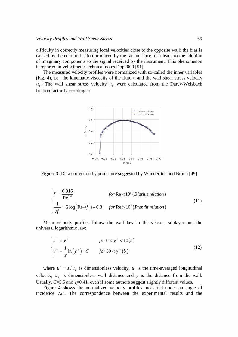
Figure 3 shows the axial time-averaged velocity u as a function of the distance from the ultrasound transducer in the sound propagation direction. The average profile was obtained from instantaneous measurements, during 100 s of acquisition and the velocities were measured at 1024 points over a depth of 30.7 mm giving a spatial resolution of 0.69 mm in the sound propagation direction. The time between two subsequent pulses was 96PRFT sμ= . Figure 3 clearly demonstrates velocimeter

Velocity Profiles and Wall Shear Stress 69

difficulty in correctly measuring local velocities close to the opposite wall: the bias is caused by the echo reflection produced by the far interface, that leads to the addition of imaginary components to the signal received by the instrument. This phenomenon is reported in velocimeter technical notes Dop2000 [51].

The measured velocity profiles were normalized with so-called the inner variables (Fig. 4), i.e., the kinematic viscosity of the fluid υ and the wall shear stress velocity uτ . The wall shear stress velocity uτ were calculated from the Darcy-Weisbach

friction factor f according to

Figure 3: Data correction by procedure suggested by Wunderlich and Brunn [49]

( )

( ) ( )

51/4

5

0.316Re 10

Re1

2log Re 0.8 Re 10

f for Blasius relation

f for Prandlt relationf

⎧ = <⎪⎪⎨⎪ = − >⎪⎩

(11)

Mean velocity profiles follow the wall law in the viscous sublayer and the

universal logarithmic law:

( )

( ) ( )

0 10

1ln 30

u y for y a

u y C for y bχ

+ + +

+ + +

⎧ = < <⎪⎨ = + <⎪⎩

(12)

where /u u uτ

+ = is dimensionless velocity, u is the time-averaged longitudinal

velocity, uτ is dimensionless wall distance and y is the distance from the wall.

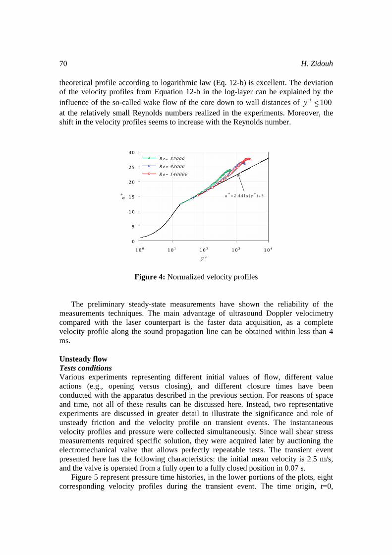
Usually, C=5.5 and χ=0.41, even if some authors suggest slightly different values. Figure 4 shows the normalized velocity profiles measured under an angle of

incidence 72°. The correspondence between the experimental results and the

70 H. Zidouh

theoretical profile according to logarithmic law (Eq. 12-b) is excellent. The deviation of the velocity profiles from Equation 12-b in the log-layer can be explained by the influence of the so-called wake flow of the core down to wall distances of 100y + <

%

at the relatively small Reynolds numbers realized in the experiments. Moreover, the shift in the velocity profiles seems to increase with the Reynolds number.

Figure 4: Normalized velocity profiles

The preliminary steady-state measurements have shown the reliability of the

measurements techniques. The main advantage of ultrasound Doppler velocimetry compared with the laser counterpart is the faster data acquisition, as a complete velocity profile along the sound propagation line can be obtained within less than 4 ms. Unsteady flow Tests conditions Various experiments representing different initial values of flow, different value actions (e.g., opening versus closing), and different closure times have been conducted with the apparatus described in the previous section. For reasons of space and time, not all of these results can be discussed here. Instead, two representative experiments are discussed in greater detail to illustrate the significance and role of unsteady friction and the velocity profile on transient events. The instantaneous velocity profiles and pressure were collected simultaneously. Since wall shear stress measurements required specific solution, they were acquired later by auctioning the electromechanical valve that allows perfectly repeatable tests. The transient event presented here has the following characteristics: the initial mean velocity is 2.5 m/s, and the valve is operated from a fully open to a fully closed position in 0.07 s.

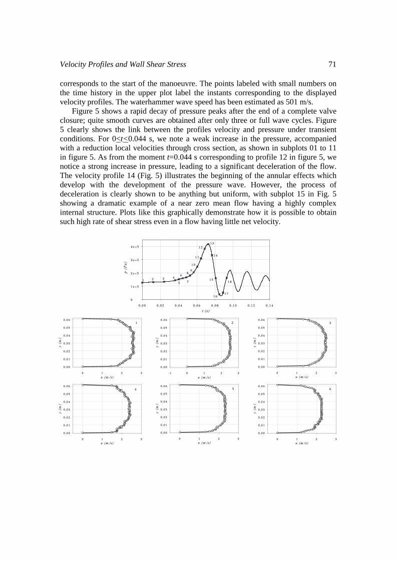
Figure 5 represent pressure time histories, in the lower portions of the plots, eight corresponding velocity profiles during the transient event. The time origin, t=0,

Velocity Profiles and Wall Shear Stress 71

corresponds to the start of the manoeuvre. The points labeled with small numbers on the time history in the upper plot label the instants corresponding to the displayed velocity profiles. The waterhammer wave speed has been estimated as 501 m/s.

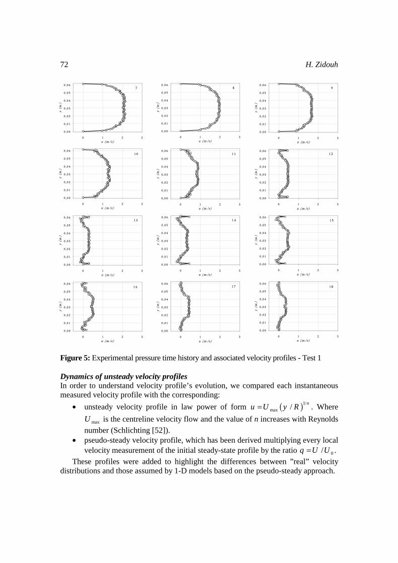
Figure 5 shows a rapid decay of pressure peaks after the end of a complete valve closure; quite smooth curves are obtained after only three or full wave cycles. Figure 5 clearly shows the link between the profiles velocity and pressure under transient conditions. For 0<t<0.044 s, we note a weak increase in the pressure, accompanied with a reduction local velocities through cross section, as shown in subplots 01 to 11 in figure 5. As from the moment t=0.044 s corresponding to profile 12 in figure 5, we notice a strong increase in pressure, leading to a significant deceleration of the flow. The velocity profile 14 (Fig. 5) illustrates the beginning of the annular effects which develop with the development of the pressure wave. However, the process of deceleration is clearly shown to be anything but uniform, with subplot 15 in Fig. 5 showing a dramatic example of a near zero mean flow having a highly complex internal structure. Plots like this graphically demonstrate how it is possible to obtain such high rate of shear stress even in a flow having little net velocity.

72 H. Zidouh

Figure 5: Experimental pressure time history and associated velocity profiles - Test 1 Dynamics of unsteady velocity profiles In order to understand velocity profile’s evolution, we compared each instantaneous measured velocity profile with the corresponding:

• unsteady velocity profile in law power of form ( )1/

max /n

u U y R= . Where

maxU is the centreline velocity flow and the value of n increases with Reynolds

number (Schlichting [52]). • pseudo-steady velocity profile, which has been derived multiplying every local

velocity measurement of the initial steady-state profile by the ratio 0/q U U= .

These profiles were added to highlight the differences between ”real” velocity distributions and those assumed by 1-D models based on the pseudo-steady approach.

Velocity Profiles and Wall Shear Stress 73

74 H. Zidouh

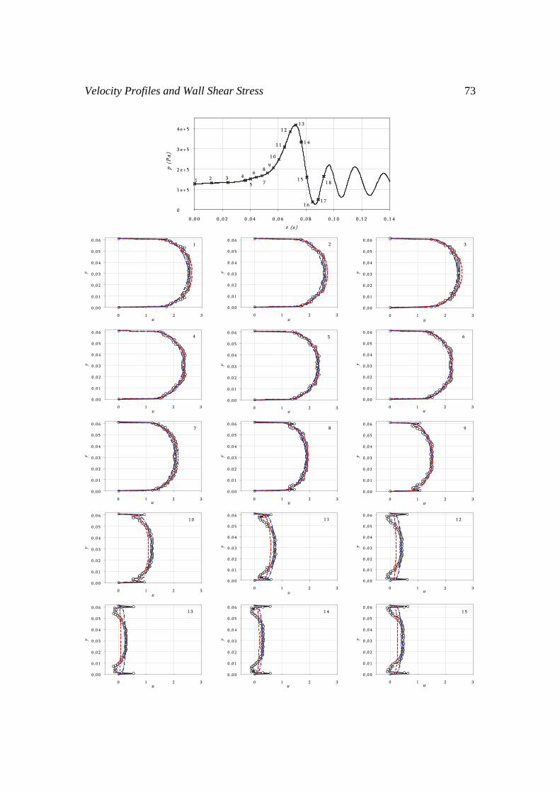
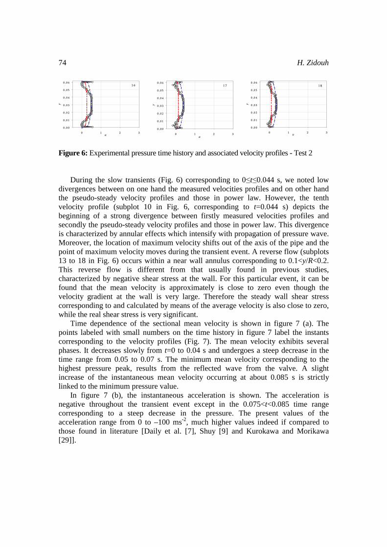
Figure 6: Experimental pressure time history and associated velocity profiles - Test 2

During the slow transients (Fig. 6) corresponding to 0≤t≤0.044 s, we noted low

divergences between on one hand the measured velocities profiles and on other hand the pseudo-steady velocity profiles and those in power law. However, the tenth velocity profile (subplot 10 in Fig. 6, corresponding to t=0.044 s) depicts the beginning of a strong divergence between firstly measured velocities profiles and secondly the pseudo-steady velocity profiles and those in power law. This divergence is characterized by annular effects which intensify with propagation of pressure wave. Moreover, the location of maximum velocity shifts out of the axis of the pipe and the point of maximum velocity moves during the transient event. A reverse flow (subplots 13 to 18 in Fig. 6) occurs within a near wall annulus corresponding to 0.1<y/R<0.2. This reverse flow is different from that usually found in previous studies, characterized by negative shear stress at the wall. For this particular event, it can be found that the mean velocity is approximately is close to zero even though the velocity gradient at the wall is very large. Therefore the steady wall shear stress corresponding to and calculated by means of the average velocity is also close to zero, while the real shear stress is very significant.

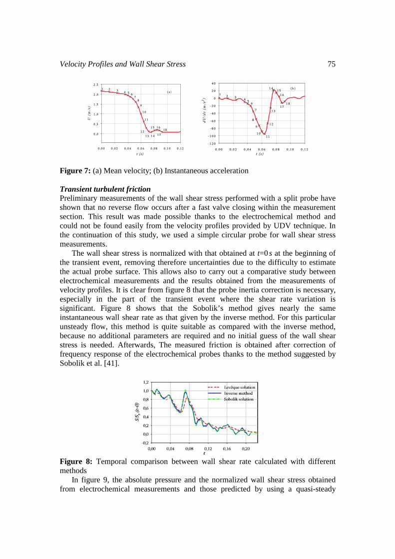
Time dependence of the sectional mean velocity is shown in figure 7 (a). The points labeled with small numbers on the time history in figure 7 label the instants corresponding to the velocity profiles (Fig. 7). The mean velocity exhibits several phases. It decreases slowly from t=0 to 0.04 s and undergoes a steep decrease in the time range from 0.05 to 0.07 s. The minimum mean velocity corresponding to the highest pressure peak, results from the reflected wave from the valve. A slight increase of the instantaneous mean velocity occurring at about 0.085 s is strictly linked to the minimum pressure value.

In figure 7 (b), the instantaneous acceleration is shown. The acceleration is negative throughout the transient event except in the 0.075<t<0.085 time range corresponding to a steep decrease in the pressure. The present values of the acceleration range from 0 to –100 ms-2, much higher values indeed if compared to those found in literature [Daily et al. [7], Shuy [9] and Kurokawa and Morikawa [29]].

Velocity Profiles and Wall Shear Stress 75

Figure 7: (a) Mean velocity; (b) Instantaneous acceleration

Transient turbulent friction Preliminary measurements of the wall shear stress performed with a split probe have shown that no reverse flow occurs after a fast valve closing within the measurement section. This result was made possible thanks to the electrochemical method and could not be found easily from the velocity profiles provided by UDV technique. In the continuation of this study, we used a simple circular probe for wall shear stress measurements.

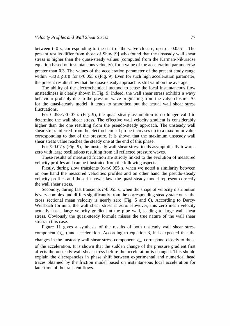
The wall shear stress is normalized with that obtained at t=0 s at the beginning of the transient event, removing therefore uncertainties due to the difficulty to estimate the actual probe surface. This allows also to carry out a comparative study between electrochemical measurements and the results obtained from the measurements of velocity profiles. It is clear from figure 8 that the probe inertia correction is necessary, especially in the part of the transient event where the shear rate variation is significant. Figure 8 shows that the Sobolik’s method gives nearly the same instantaneous wall shear rate as that given by the inverse method. For this particular unsteady flow, this method is quite suitable as compared with the inverse method, because no additional parameters are required and no initial guess of the wall shear stress is needed. Afterwards, The measured friction is obtained after correction of frequency response of the electrochemical probes thanks to the method suggested by Sobolik et al. [41].

Figure 8: Temporal comparison between wall shear rate calculated with different methods

In figure 9, the absolute pressure and the normalized wall shear stress obtained from electrochemical measurements and those predicted by using a quasi-steady

76 H. Zidouh

assumption are displayed. The points labeled with small numbers on the time history in this figure label the instants corresponding to the displayed velocity profiles (Fig. 5). From the measurements, the values of k were computed and plotted against ø in figure 10, for different range of t.

Figure 9: Wall shear stress and pressure distributions during a transient event

Figure 10: Plot of k against ø : (a) t<0.055 s, (b) 0.055<t<0.07 s, (c) t>0.07 s

The results show that the wall shear stress measured with the electrochemical signals and that predicted by a quasi-steady model are close for the time range

Velocity Profiles and Wall Shear Stress 77

between t=0 s, corresponding to the start of the valve closure, up to t=0.055 s. The present results differ from those of Shuy [9] who found that the unsteady wall shear stress is higher than the quasi-steady values (computed from the Karman-Nikuradse equation based on instantaneous velocity), for a value of the acceleration parameter φ greater than 0.3. The values of the acceleration parameter of the present study range within 30 0φ− ≤ ≤ for t<0.055 s (Fig. 9). Even for such high acceleration parameter, the present results show that the quasi-steady approach is still valid on the average.

The ability of the electrochemical method to sense the local instantaneous flow unsteadiness is clearly shown in Fig. 9. Indeed, the wall shear stress exhibits a wavy behaviour probably due to the pressure wave originating from the valve closure. As for the quasi-steady model, it tends to smoothen out the actual wall shear stress fluctuations.

For 0.055<t<0.07 s (Fig. 9), the quasi-steady assumption is no longer valid to determine the wall shear stress. The effective wall velocity gradient is considerably higher than the one resulting from the pseudo-steady approach. The unsteady wall shear stress inferred from the electrochemical probe increases up to a maximum value corresponding to that of the pressure. It is shown that the maximum unsteady wall shear stress value reaches the steady one at the end of this phase.

For t>0.07 s (Fig. 9), the unsteady wall shear stress tends asymptotically towards zero with large oscillations resulting from all reflected pressure waves.

These results of measured friction are strictly linked to the evolution of measured velocity profiles and can be illustrated from the following aspects:

Firstly, during slow transients 0≤t≤0.055 s, when we noted a similarity between on one hand the measured velocities profiles and on other hand the pseudo-steady velocity profiles and those in power law, the quasi-steady model represent correctly the wall shear stress.

Secondly, during fast transients t>0.055 s, when the shape of velocity distribution is very complex and differs significantly from the corresponding steady-state ones, the cross sectional mean velocity is nearly zero (Fig. 5 and 6). According to Darcy-Weisbach formula, the wall shear stress is zero. However, this zero mean velocity actually has a large velocity gradient at the pipe wall, leading to large wall shear stress. Obviously the quasi-steady formula misses the true nature of the wall shear stress in this case.

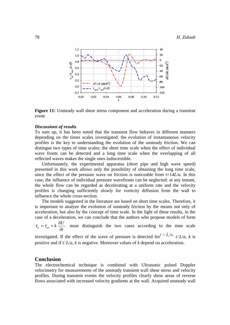
Figure 11 gives a synthesis of the results of both unsteady wall shear stress component ( wuτ ) and acceleration. According to equation 3, it is expected that the

changes in the unsteady wall shear stress component wuτ correspond closely to those

of the acceleration. It is shown that the sudden change of the pressure gradient first affects the unsteady wall shear stress before the acceleration is changed. This should explain the discrepancies in phase shift between experimental and numerical head traces obtained by the friction model based on instantaneous local acceleration for later time of the transient flows.

78 H. Zidouh

Figure 11: Unsteady wall shear stress component and acceleration during a transient event Discussions of results To sum up, it has been noted that the transient flow behaves in different manners depending on the times scales investigated: the evolution of instantaneous velocity profiles is the key to understanding the evolution of the unsteady friction. We can distingue two types of time scales: the short time scale when the effect of individual wave fronts can be detected and a long time scale when the overlapping of all reflected waves makes the single ones indiscernible.

Unfortunately, the experimental apparatus (short pipe and high wave speed) presented in this work allows only the possibility of obtaining the long time scale, since the effect of the pressure wave on friction is noticeable from t=14L/a. In this case, the influence of individual pressure wavefronts can be neglected: at any instant, the whole flow can be regarded as decelerating at a uniform rate and the velocity profiles is changing sufficiently slowly for vorticity diffusion from the wall to influence the whole cross-section.

The models suggested in the literature are based on short time scales. Therefore, it is important to analyze the evolution of unsteady friction by the means not only of acceleration, but also by the concept of time scale. In the light of these results, in the case of a deceleration, we can conclude that the authors who propose models of form

w ws

Uk

tτ τ ∂= +

∂ must distinguish the two cases according to the time scale

investigated. If the effect of the wave of pressure is detected for t L/a, k is positive and if t L/a, k is negative. Moreover values of k depend on acceleration.

Conclusion The electrochemical technique is combined with Ultrasonic pulsed Doppler velocimetry for measurements of the unsteady transient wall shear stress and velocity profiles. During transient events the velocity profiles clearly show areas of reverse flows associated with increased velocity gradients at the wall. Acquired unsteady wall

Velocity Profiles and Wall Shear Stress 79

shear stress by using the electrochemical method provides complementary and additional near wall information to the velocity profiles and demonstrates the complex nature of the near wall flow field. The present results show that the quasi-steady model for predicting the wall shear stress is valid for a wide ranging acceleration parameter and that the unsteady friction coefficient is unlikely to be constant for a non uniform decelerating flow. In the light of this study, the electrochemical method seems to be the most appropriate technique that could contribute to a better understanding of transient flow dynamics and energy dissipation. Further experimental measurements based on the electrochemical method should be performed in a longer pipe allowing both short and long time scales.

Nomenclature a water hammer wave speed. A active surface of the electrochemical probe. d diameter of the circular sensor (m). D inner pipe diameter. F Darcy-Weisbach friction factor. G gravitational acceleration. I limiting diffusion current. K unsteady friction factor. K mass transfer coefficient. L pipe length. n number of electrons involved in the redox reaction. R inner pipe radius. S wall shear rate (s-1). U mean velocity in the cross-section. C* Vardy’s shear decay coefficient. Δ diffusivity. Φ Faraday’s constant. C0 concentration of the active ions. Re Reynolds number, = DU/υ. τw wall shear stress. τws quasi-steady wall shear stress. τwu unsteady wall shear stress. ρ density of fluid. υ kinematic viscosity. Μ dynamic viscosity. uτ friction velocity, = /wτ ρ =(ms-1).

80 H. Zidouh

References [1] Brunone, B., Karney, B., Mecarelli, M., and Ferrante, M., 2000. “Velocity

profiles and unsteady pipe friction in transient flow”. J. water ressources planning and mangement, 126(4), pp. 236–244.

[2] Zidouh, H.,William-Louis, M., and Labraga, L., 2007. “Etude de l’écoulement turbulent transitoire dans une conduite”. Proc., 18ème Congres Français de Mécanique, Grenoble, France.

[3] Eichinger, P., and Lein, G., 1992. “The influence of friction on unsteady pipe flow”. Proceeding of the Int. Conf. on Unsteady Flow and Fluid Transients, B. ed., Balkema, Rotterdam, The Netherlands, Durham, Uk, pp. 41–50.

[4] Bergant, A., Simpson, A., and Vitkosky, J., 2001. “Developments in unsteady pipe flow friction modelling”. Journal of Hydraulic Research, 39(3), pp. 249–257.

[5] Cocchi, G., 1989. “Esperimento sulla resistenza al deflusso con moto vario in un tubo”. Atti della Academia delle Scienze dell’Instituto di Bologna, 14, pp. 203–210.

[6] Hino, M., Masaki, S., and Shuji, T., 1976. “Experiments on transition to turbulence in an oscillatory pipe flow”. Journal of Fluid Mechanics, 75, pp. 193–207.

[7] Daily, W., Hankey, W., Olive, R., and Jordan, J., 1956. “Resistance coefficients for accelerated and decelerated flows through smooth tubes and orifices”. Transactions of ASME, 78, pp. 1071–1077.

[8] Cartsens, M., and Roller, J., 1959. “Boundary-shear stress in unsteady turbulent pipe flow”. Journal of the hydraulics division, ASCE, 85, pp. 67–81.

[9] Shuy, E., 1996. “Wall shear stress in accelerating and decelerating turbulent pipe flows”. Journal of Hydraulic Research, 34(2), pp. 173–183.

[10] Safwat, H., and Van der Polder, J., 1973. “Friction-frequency dependence for oscillatory flows in circular pipes”. Journal of Hydraulics division, ASCE, 99(HY11), pp. 1933–1945.

[11] Brunone, B., Golia, U., and Greco, M., 1991. “Some remarks on the momentum equation for fast transients”. Int. Meeting on Hydraulic Transients with Column Separation, 9th Round Table, IAHR, Valencia, Spain, pp. 201–209.

[12] Vennatrø, B., 1996. “Unsteady friction in pipelines”. Proc., XVIII IAHR Symposium on Hydraulic Machinery and Cavitation, Valencia, Spain, 2, pp. 819–826.

[13] Svingen, B., 1997. “Rayleigh damping as an approximate model for transient hydraulic pipe friction”. Proc., 8th Int. Meet. on the Behaviour of Hydraulic Machinery under Steady Oscillatory Conditions, IAHR, Chatou, France, pp. Paper F–2.

[14] Zielke, W., 1968. “Frequency-dependent friction in transient pipe flow”. Journal of Basic Engineering, ASME, 90, pp. 109–115.

Velocity Profiles and Wall Shear Stress 81

[15] Trikha, A., 1975. “An efficient method for simulating frequency-dependent friction in transient liquid flow”. Journal of Fluids Engineering, ASME, 97(1), pp. 97–105.

[16] Vardy, A., Hwang, K., and Brown, J., 1993. “A weighting function model of transient turbulent pipe flow”. Journal of Hydraulic Research, 31, pp. 533–548.

[17] Vardy, A., and Brown, J., 1995. “Transient, turbulent, smooth pipe friction”. Journal of Hydraulic Research, IAHR, 33(4), pp. 435–456.

[18] Vardy, A., and Brown, J., 1996. “On turbulent, unsteady, smooth-pipe friction”. Proc., 7th Int. Conf. on Pressure Surges and Fluid Transients in Pipelines and Open Channels, BHR Group, Harrogate, England, p. 289.

[19] Vardy, A., and Brown, J., 2003. “Transient turbulent friction in smooth pipe flows”. Journal of Sound and Vibration, 259(5), pp. 1011–1036.

[20] Vardy, A., and Brown, J., 2004. “Transient turbulent friction in fully rough pipe flows”. Journal of Sound and Vibration, 270, pp. 233–257.

[21] Vardy, A., and Hwang, K., 1991. “A characteristics model of transient friction”. Journal of Hydraulic Research, 29(5), pp. 669–684.

[22] Silva-Araya, W., and Chaudhry, M., 1997. “Computation of energy dissipation in transient flow”. Journal of Hydraulic Engineering, 123(2), pp. 108–115.

[23] Pezzinga, G., 1999. “Quasi-2d model for unsteady flow in pipe networks”. Journal of Hydraulic Engineering, ASCE, 125(7), pp. 676–685.

[24] Vardy, A., and Brown, J., 1997. “Discussion on «wall shear stress in accelerating and decelerating turbulent pipe flows»”. Journal of Hydraulic Research, IAHR, 35(1), pp. 137–139.

[25] Brunone, B., and Golia, U., 1991. “Some considerations on velocity profiles in unsteady pipe flows”. Proc., Int. Conf. on “Entropy and Energy Dissipation in Water Resources”, Maratea, Italy, V.O. Singh and M. Fiorentino, Eds., pp. 281–487.

[26] Greco, M., 1990. “Some recent findings on column separation during water hammer”. Excerpta, G.N.I., Liberia Progetto Ed. Padua, Italy, 5, pp. 261–272.

[27] Brunone, B., Golia, U., and Greco, M., 1991. “Modeling of fast transients by numerical methods”. Int. Meeting on Hydraulic Transients with Column Separation, 9th Round Table, IAHR, Valencia, Spain, pp. 273–281.

[28] Schohl, G., 1993. “Improved approximate method for simulating frequency-dependent friction in transient laminar flow”. Journal of Fluids Engineering, 115, pp. 420–424.

[29] Kurokawa, J., and Morikawa, M., 1986. “Accelerated and decelerated flows in a circular pipe”. 1st Report, Velocity profile and friction coefficient Bullettin of JSME, 29, pp. 758–765.

[30] Hanratty, T., and Campbell, J., 1983. “Measurements of wall shear stress”. In. Fluid Mechanics. Measurements (ed. R.J. Goldstein), pp. 559–615.

[31] Reiss, L., and Hanratty, T., 1963. “An experimental study of the unsteady nature of the viscous sub-layer”. A.I.Ch.E Journal, 9, pp. 154–160.

82 H. Zidouh

[32] Lebouché, M., 1968. “Contribution l’étude des mouvements turbulents par la méthode polarographique”. Thèse de Doctorat ès sciences, Nancy I, Nancy, France.

[33] Cognet, G., 1968. “Contribution à l’étude du mouvement de couette par la méthode polarographique”. PhD thesis.

[34] Son, J., and Hanratty, T., 1969. “Velocity gradients at the wall for flow around a cylinder at reynolds number from 5:103 to 106”. Journal of Fluid Mechanics, 35, pp. 353–368.

[35] Py, B., and Gosse, J., 1969. “Sur la réalisation d’une sonde polarographique pariétale sensible à la vitesse et à la direction de l’écoulement”. Comptes Rendus Ac. Sc. Paris, tome 269, pp. 401–404.

[36] Levêque, M., 1928. “Les lois de transmission de la chaleur par convection”. Ann. Mines, 13, pp. 381–412.

[37] Rehimi, F., Aloui, F., Nasrallah, S. B., Doubliez, L., and Legrand, J., 2006. “Inverse method for electrodiffusional diagnostics of flows”. International Journal of Heat and Mass Transfer, 49, pp. 1242–1254.

[38] Mitchell, J., and Hanratty, T., 1966. “A study of turbulence at a wall using an electrochemical wall-stress meter”. Journal of Fluid Mechanics, 26, pp. 199–221.

[39] Deslouis, C., Gil, O., and Tribollet, B., 1990. “Frequency response of electrochemical sensors to hydrodynamic fluctuations”. Journal of Fluid Mechanics, 215, pp. 85–100.

[40] Maquinghen, T., 1999. “Métrologie tridimensionnelle instationnaire à l’aide de la méthode polarographique”. PhD thesis.

[41] Sobolik, V., Wein, O., and Cermak, J., 1987. “Simultaneous measurement of film thickness and wall shear stress in wavy flow of non-newtonian liquids”. Collection Czechoslovak Chem. Comun., 52, pp. 913–928.

[42] Wein, O., 1981. “On the transient levêque’s problem with application in electrochemistry”. Colln Czech Chem Commun, 46, pp. 3209–3220.

[43] Tihon, J., Legrand, J., Aouabed, H., and Legentilhomme, P., 1995. “A characteristics model of transient friction”. Technical Notes, Experiments in Fluids, 20, pp. 131–134.

[44] Sobolik, V., Tihon, J., and Wein, O., 1998. “Calibration of electrodiffusion friction probes using a voltage-step transient”. Journal of Applied Electrochemistry, 28, pp. 329–335.

[45] Mao, Z., and Hanratty, J., 1991. “Analysis of wall shear stress probes in large amplitude unsteady flows”. Int. J. Heat Mass Transfer, 34, pp. 281–290.

[46] Kaiping, P., 1983. “Unsteady forced convective heat transfer from a hot film in nonreversing and reversing shear flow”. Int J. Heat Mass Transfer, 26, pp. 545–557.

[47] Zidouh, H., 2007. “Etude expérimentale du frottement pariétal instationnaire”. PhD thesis, Thèse de Doctorat, Université de Valenciennes, Valenciennes, France.

[48] Takeda, Y., 1986. “Velocity measurement by ultrasound doppler shift method”. International of Journal Heat and Fluid Flow, 7(4), pp. 313–318.

Velocity Profiles and Wall Shear Stress 83

[49] Wunderlich, J., and Brunn, P., 2000. “A wall layer correction for ultrasound measurement in tube flow: comparison between theory and experiment”. Flow Measurement and Instrumentation, 11, pp. 63–69.

[50] Nowak, M., 2002. “Wall shear stress measurement in a turbulent pipe flow using ultrasound doppler velocimetry”. Experiments in fluids, 33, pp. 249–255.

[51] S.A. SIGNAL PROCESSING, 2003. DOP2000 User’s manual. Switzerland. [52] Schlichting, H., 1979. Boundary Layer Theory, 7th ed. McGraw-Hill, New

York.