Embed Size (px)
Citation preview

Distrib. Comput. (2000) 13: 155–186
c© Springer-Verlag 2000
Verification of the randomized consensus algorithmof Aspnes and Herlihy: a case study
Anna Pogosyants1, Roberto Segala2, Nancy Lynch1
1 Laboratory for Computer Science, Massachusetts Institute of Technology, Cambridge, MA 02139, USA (e-mail: [email protected])2 Dipartimento di Scienze dell’Informazione, Universita di Bologna, Piazza di Porta San Donato 5, 40127 Bologna, Italy(e-mail: [email protected])
Received: February 1999 / Accepted: March 2000
This paper is written in memory of Anna Pogosyants, who died in a car crash in December 1995 while working on this project forher Ph.D. dissertation.
Summary. The Probabilistic I/O Automaton model of [31]is used as the basis for a formal presentation and proof of therandomized consensus algorithm of Aspnes and Herlihy. Thealgorithm guarantees termination within expected polynomialtime. The Aspnes-Herlihy algorithm is a rather complex algo-rithm. Processes move through a succession of asynchronousrounds, attempting to agree at each round. At each round, theagreement attempt involves a distributed random walk. Thealgorithm is hard to analyze because of its use of nontrivialresults of probability theory (specifically, random walk the-ory which is based on infinitely many coin flips rather thanon finitely many coin flips), because of its complex setting,including asynchrony and both nondeterministic and proba-bilistic choice, and because of the interplay among severaldifferent sub-protocols. We formalize the Aspnes-Herlihy al-gorithm using probabilistic I/O automata. In doing so, we de-compose it formally into three subprotocols: one to carry outthe agreement attempts, one to conduct the random walks,and one to implement a shared counter needed by the randomwalks. Properties of all three subprotocols are proved sepa-rately, and combined using general results about automatoncomposition. It turns out that most of the work involves prov-ing non-probabilistic properties (invariants, simulation map-pings, non-probabilistic progress properties, etc.). The prob-abilistic reasoning is isolated to a few small sections of theproof. The task of carrying out this proof has led us to de-velop several general proof techniques for probabilistic I/Oautomata. These includeways to combineexpectations for dif-ferent complexity measures, to compose expected complex-ity properties, to convert probabilistic claims to determinis-tic claims, to use abstraction mappings to prove probabilisticproperties, and to apply random walk theory in a distributedcomputational setting. We apply all of these techniques to an-alyze the expected complexity of the algorithm.
Key words: Randomized consensus – Probabilistic automata– Verification – Performance analysis
Supported by AFOSR-ONR contract F49620-94-1-0199, by ARPAcontracts N00014-92-J-4033 and F19628-95-C-0118, and by NSFgrant 9225124-CCR.
1 Introduction
With the increasing complexity of distributed algorithms thereis an increasing need for mathematical tools for analysis. Al-though there are several formalisms and tools for the analysisof ordinary distributed algorithms, there are not as many pow-erful tools for the analysis of randomization within distributedsystems. This paper is part of a project that aims at develop-ing the right math tools for proving properties of complicatedrandomized distributed algorithms and systems. The tools wewant to develop should be based on traditional probabilitytheory, but at the same time should be tailored to the com-putational setting. Furthermore, the tools should have goodfacilities for modular reasoning due to the complexity of thesystems to which they should be applied. The types of mod-ularity we are looking for include parallel composition andabstraction mappings, but also anything else that decomposesthe math analysis.
We develop our tools by analyzing complex algorithmsof independent interest. In this paper we analyze the random-ized consensus algorithm of Aspnes and Herlihy [5], whichguarantees termination within expected polynomial time. TheAspnes-Herlihy algorithm is a rather complex algorithm. Pro-cessesmove through a succession of asynchronous rounds, at-tempting to agree at each round. At each round, the agreementattempt involves a distributed random walk. The algorithm ishard to analyze because of its use of nontrivial results of prob-ability theory (specifically, random walk theory), because ofits complex setting, including asynchrony and both nondeter-ministic and probabilistic choice, and because of the interplayamong several different sub-protocols.
We formalize the Aspnes-Herlihy algorithm using proba-bilistic I/O automata [31]. In doing so, we decompose it for-mally into three subprotocols: one to carry out the agreementattempts, one to conduct the random walks, and one to imple-ment a shared counter needed by the randomwalks. Propertiesof all three subprotocols are proved separately, and combinedusing general results about automaton composition. It turnsout that most of the work involves proving non-probabilisticproperties (invariants, simulationmappings, non-probabilistic

156 A. Pogosyants et al.
progress properties, etc.). The probabilistic reasoning is iso-lated to a few small sections of the proof.
The taskof carryingout thisproofhas ledus todevelopsev-eral general proof techniques for probabilistic I/O automata.These includeways tocombineexpectations for different com-plexitymeasures, to compose expected complexity properties,to convert probabilistic claims to deterministic claims, to useabstraction mappings to prove probabilistic properties, and toapply random walk theory in a distributed computational set-ting. We apply all of these techniques to analyze the expectedcomplexity of the algorithm.
Previous work on verification of randomized distributedalgorithms includes [28], where the randomized diningphilosophers algorithm of [22] is shown to guarantee progresswith probability 1, [24,29], where the algorithm of [22] isshown to guarantee progress within expected constant time,and [2], where the randomized self-stabilizingminimumspan-ning tree algorithm of [3] is shown to guarantee stabilizationwithin an expected time proportional to the diameter of a net-work. The analysis of [28] is based on converting a probabilis-tic property into a property of some of the computations of analgorithm (extreme fair computations); the analysis of [24,29,2] is based on part of the methodology used in this paper. An-other verification technique, based on the so called scheduler-luck games, is presented in [14]. Other work is based on theextension of model checking techniques to the probabilisticcase [32,19,10] and on the extension of predicate transform-ers to the probabilistic case [27].
Prior to the algorithm of Aspnes and Herlihy, the bestknown randomizedalgorithm for consensuswith sharedmem-ory was due to Abrahamson [1]. The algorithm has expo-nential expected running time. The algorithm of Aspnes andHerlihy was improved by Attiya, Dolev, and Shavit [7] byeliminating the use of unbounded counters needed for the ran-dom walk. Further improvements were proposed by Aspnes[4], by Dwork, Herlihy, Plotkin, and Waarts [15], by Brachaand Rachman [11] (O(n2 log n) operations), and by Aspnesand Waarts [6] (O(n log2 n) operations per processor). Otherimprovements were proposed by Aumann and Bender [9](O(n log2 n) operations), by Chandra [12] (O(log2 n) workper processor), and by Aumann [8] (O(log n) work per pro-cessor) by imposing appropriate restrictions on the power ofthe adversary.
The rest of the paper is organized as follows. Section 2presents the basic theoretical tools for our analysis, includ-ing probabilistic I/O automata, abstract complexity measures,progress statements and refinementmappings; Sect. 3 presentsa coin lemma for random walks and a result about the ex-pected complexity of a random walk within a probabilisticI/O automaton; Sect. 4 presents the algorithm of Aspnes andHerlihy and describes formally the module that carries outthe agreement attempts; Sects. 5 and 6 prove that the Aspnes-Herlihy algorithm satisfies the validity and agreement proper-ties; Sect. 7 proves several progress properties of the algorithmthat arenot basedonanyprobabilistic argument;Sect. 8 provesthe probabilistic progress properties of the algorithm by usingthe results of Sect. 7; Sect. 9 builds the module that conductsthe random walk; Sect. 10 builds the shared counter neededin Sect. 9; Sect. 11 derives the termination properties of thealgorithm, where the complexity is measured in terms of ex-
pected number of rounds; Sect. 12 studies the expected timecomplexity of the algorithm; Sect. 13 gives some concludingremarks and discusses the kinds of modularization that we usein the proof.
Part I: The underlying theory
2 Formal model and tools
In this section we introduce the formalism that we use in thepaper. We start with ordinary I/O automata following the styleof [25,23]; then we move to probabilistic I/O automata byadding the input/output structure to the probabilistic automataof [31]. We describe methods to handle complexity measureswithin probabilistic automata, and we present progress state-ments as a basic tool for the complexity analysis of a prob-abilistic system. Finally, we describe verification techniquesbased on refinements and traces.
2.1 I/O automata
An I/O automatonA consists of five components:
• A setStates(A) of states.• A non-empty setStart(A) ⊆ States(A) of start states.• An action signatureSig(A) = (in(A), out(A), int(A)),wherein(A), out(A)andint(A)aredisjoint sets:in(A) isthe set of input actions,out(A) is the set of output actions,andint(A) is the set of internal actions.
• A transition relationTrans(A)⊆States(A)×Actions(A)×States(A), whereActions(A) denotes the setin(A) ∪out(A) ∪ int(A), such that for each states of States(A)and each input actiona of in(A) there is a states′ suchthat(s, a, s′) is an element ofTrans(A). The elements ofTrans(A) are calledtransitions, andA is said to beinputenabled.
• A task partitionTasks(A), which is an equivalence rela-tion onint(A)∪ out(A) that has at most countably manyequivalence classes. An equivalence class ofTasks(A) iscalled ataskof A.
In the rest of the paper we refer to I/O automata as automata.A states of A is said toenablea transition if there is
a transition(s, a, s′) in Trans(A); an actiona is said to beenabledfrom s if there is a transition(s, a, s′) in Trans(A);a taskT ofA is said to beenabledfrom s if there is an actiona ∈ T that is enabled froms.
An execution fragmentof an automatonA is a sequenceα of alternating states and actions ofA starting with a state,and, ifα is finite, endingwith a state,α = s0a1s1a2s2..., suchthat for eachi ≥ 0 there exists a transition(si, ai+1, si+1) ofA. Denote byfstate(α) the first state ofα and, ifα is finite,denote bylstate(α) the last state ofα. Denote byfrag∗(A)the set of finite execution fragments ofA. An executionis anexecution fragment whose first state is a start state.
An execution fragmentα is said to befair iff the followingconditions hold for every taskT of A:
1. if α is finite thenT is not enabled inlstate(α);2. if α is infinite, then either actions fromT occur infinitely
many times inα, orα contains infinitelymanyoccurrencesof states from whichT is not enabled.

Verification of the randomized consensus algorithm of Aspnes and Herlihy: a case study 157
A states ofA is reachableif there exists a finite execution ofAthat ends ins. Denote byrstates(A) the set of reachable statesofA. A propertyφ of states is said to bestablefor an executionfragmentα = s0a1s1 · · · if, onceφ is true,φ remains true inall later states. That is, for everyi ≥ 0, φ(si) ⇒ ∀j≥iφ(sj).
A finite execution fragmentα1 = s0a1s1 · · · ansn of Aand an execution fragmentα2 = snan+1sn+1 · · · ofA can beconcatenated. The concatenation, writtenα1
α2, is the exe-cution fragments0a1s1 · · · ansnan+1sn+1 · · ·. An executionfragmentα1 ofA is aprefixof an execution fragmentα2 ofA,writtenα1 ≤ α2, iff either α1 = α2 or α1 is finite and thereexists an execution fragmentα′
1 ofA such thatα2 = α1 α′
1.If α = α1
α2, thenα2 is called asuffixofα, and it is denotedalternatively byαα1.
2.2 Probabilistic I/O automata
2.2.1 Preliminaries on probability theory
In this section we recall some basic definitions and resultsfrom probability theory. The reader interested in more detailsis referred to any book on probability theory.
A probability spaceis a triplet(Ω,F , P ) where
1. Ω is a set, also called thesample space,2. F is a collection of subsets ofΩ that is closed under com-
plement and countable union and such thatΩ ∈ F , alsocalled aσ-field, and
3. P is a function fromF to [0, 1] such thatP [Ω] = 1and such that for any collectionCii of at most count-ably many pairwise disjoint elements ofF , P [∪iCi] =∑
i P [Ci].
The pair(Ω,F) is called ameasurable space, and themeasureP is called aprobability measure.
A probability space(Ω,F , P ) is discreteif F = 2Ω andfor eachC ⊆ Ω,P [C] =
∑x∈C P [x]. For any arbitrary set
X, letProbs(X) denote the set of discrete probability distri-butions whose sample space is a subset ofX and such that allthe elements of the sample space have a non-zero probability.
A function f : Ω1 → Ω2 is said to bemeasurablefrom(Ω1,F1) to (Ω2,F2) if for eachE ∈ F2, f−1(E) ∈ F1.Given a probability space(Ω1,F1,P1), a measurable space(Ω2,F2), and a measurable functionf from (Ω1,F1) to (Ω2,F2), let f(P1), the image measureof P1, be the measure de-fined on(Ω2,F2) as follows: for eachE ∈ F2, f(P1)(E) =P1(f−1(E)). Standard measure theory arguments show that(Ω2,F2, P2) is a probability space. If(Ω,F , P ) is discrete,then we can definef((Ω,F , P )) as(f(Ω), 2f(Ω), f(P )).
For notational convenience we denote a probability space(Ω,F , P ) by P. We also use primes and indices that carryover automatically to the components of a probability space.Thus, for example,P ′
i denotes(Ω′i,F ′
i , P′i ).
Given aprobability spaceP anda setX, we abusenotationand we writeP [X] even ifX contains elements that are notin Ω. By writing P [X] we mean implicitlyP [X ∩ Ω]. Also,given an elementx, we writeP [x] for P [x].
Given two discrete probability spacesP1 andP2, definethe productP1 ⊗ P2 of P1 andP2 to be the triplet(Ω1 ×Ω2, 2Ω1×Ω2 , P1 ⊗ P2), where, for each(x1, x2) ∈ Ω1 ×Ω2,P1 ⊗ P2[(x1, x2)] = P1[x1]P2[x2].
We conclude with some notions about random variablesthatareneeded insomeof theproofsofour results. Let(,F)be a measurable space with the real numbers as sample space.Given a probability spaceP, a random variableX for P isa measurable function from(Ω,F) to (,F). As an exam-ple, a random variable could be the function that expressesthe complexity of each element ofΩ. It is possible to studythe expected valueof a random variable, that is, the aver-age complexity of the elements ofΩ, as follows:E[X] =∑
x∈Ω X(x)P [x].LetP beaprobability spaceand letX bea randomvariable
for P. For a natural numberi ≥ 0, let the expressionX ≥ idenote the eventx ∈ Ω | X(x) ≥ i. Then the followingtwo useful properties are valid.
1. If the rangeofX is thesetof natural numbers, thenE[X] =∑i>0 P [X ≥ i].
2. E[X] ≥∑i>0 P [X ≥ i].
2.2.2 Probabilistic I/O automata
A probabilistic I/OautomatonM consists of five components:
• A setStates(M) of states.• A non-empty setStart(M) ⊆ States(M) of start states.• An action signatureSig(M).• A transition relationTrans(M) ⊆ States(M)×Actions
(M) × Probs(States(M)) such that for each states ofStates(M)andeach input actionaof in(M) there is a dis-tributionP such that(s, a,P) is an element ofTrans(M).We say thatM is input-enabled.
• A task partitionTasks(M), which is an equivalence re-lation on int(M) ∪ out(M) that has at most countablymany equivalence classes.
In the rest of the paper we refer to probabilistic I/O automataas probabilistic automata. Probabilistic I/O automata are sim-ilar in structure to the probabilistic automata of [30], the con-current labeled Markov chains of [32], and Markov decisionprocesses [13]. In this paper probabilistic I/O automata areviewed as an extension of I/O automata, and thus the notationand the results that we present are chosen along the lines of[25].
Execution fragments and executions are defined similarlyto the non-probabilistic case. Anexecution fragmentof Mis a sequenceα of alternating states and actions ofM start-ing with a state, and, ifα is finite ending with a state,α =s0a1s1a2s2..., such that for eachi ≥ 0 there exists a transition(si, ai+1,P) of M such thatsi+1 ∈ Ω. All the terminologythat is used for executions in the non-probabilistic case appliesto the probabilistic case as well.
2.2.3 Probabilistic executions
An execution fragment ofM is the result of resolving boththe probabilistic and the nondeterministic choices ofM . Ifonly the nondeterministic choices are resolved, then we ob-tain a stochastic process, which we call aprobabilistic exe-cution fragmentof M . From the point of view of the studyof algorithms, the nondeterminism is resolved by anadver-sary that chooses a transition to schedule based on the past

158 A. Pogosyants et al.
history of the system. A probabilistic execution is the resultof the action of some adversary that is allowed to know ev-erything about the past but nothing about the future. Thus,the adversaries that we model cannot predict the values of fu-ture coin flips. These adversaries are called policies within thetheory of Markov Decision Processes. A probabilistic execu-tion can be thought of as the result of unfolding the transitionrelation of a probabilistic automaton and then choosing onetransition for each state of the unfolding. We also allow an ad-versary to use randomization in its choices, that is, a transitionto be chosen probabilistically. This models the fact that theenvironment of a probabilistic automaton may provide inputrandomly. We remark that from the point of view of the studyof an algorithm (how long it takes for the algorithm to ter-minate) randomized adversaries are not more powerful thannon-randomized adversaries [20,31]. However, randomizedadversaries are fundamental for the study of compositionalverification techniques as we do in this paper.
Formally, aprobabilistic execution fragmentH of a prob-abilistic automatonM consists of four components.
• A set of statesStates(H) ⊆ frag∗(M); let q range overthe states ofH;
• A signatureSig(H) = Sig(M);• A singleton setStart(H) ⊆ States(M);• A transition relationTrans(H) ⊆ States(H) × Probs
((Actions(H)×States(H))∪δ)such that for each tran-sition(q,P)ofH there isa family(lstate(q), ai,Pi)i≥0of transitions ofM and a familypii≥0 of probabilitiessatisfying the following properties:1.∑
i≥0 pi ≤ 1,2. P [δ] = 1−∑i≥0 pi, and3. for each actiona and state s, P [(a, qas)] =∑
i|ai=a piPi[s].
Furthermore, each state ofH is reachable, where reachabil-ity is defined analogously to the notion of reachability forprobabilistic automata after defining an execution of a proba-bilistic execution fragment in the obviousway. AprobabilisticexecutionH of a probabilistic automatonM is a probabilis-tic execution fragment ofM whose start state is a state ofStart(M).
A probabilistic execution is like a probabilistic automaton,except that within a transition it is possible to choose proba-bilistically over actions as well. Furthermore, a transition maycontain a special symbolδ, which corresponds to not schedul-ing any transition. In particular, it is possible that from a stateq a transition is scheduled only with some probabilityp < 1.In such a case the probability ofδ is 1− p.
The reader familiar with stochastic processes or MarkovDecision Processes may be confused by the terminology in-troduced so far since an adversary should be referred to asa policy, a probabilistic execution as a probabilistic tree, andan execution as a trace. The naming convention that we havechosen originates from the theory of I/O automata, which is incontrast with the naming convention of stochastic processes.We have decided to follow the I/O automata convention be-cause we are extending to the probabilistic case techniquesthat are typical of I/O automata.
We now describe the probability space associated witha probabilistic execution fragment, which is a standard con-struction for stochastic processes. Given a probabilistic exe-
cution fragmentH, the sample spaceΩH is the limit closureof States(H), where the limit is taken under prefix ordering.Theσ-fieldFH is the smallestσ-field that contains the set ofconesCq, consisting of those executions ofΩH havingq as aprefix. The probability measurePH is the unique extension ofthe probability measure defined on cones as follows:PH [Cq]is the product of the probabilities of each transition ofH lead-ing to q. It is easy to show that there is a unique probabilitymeasure having the property above, and thus(ΩH ,FH , PH)is a well defined probability space.
An eventE of H is an element ofFH . An eventE iscalledfinitely satisfiableif it can be expressed as a union ofcones. A finitely satisfiable event can be represented by a setof incomparable states ofH, that is, by a setΘ ⊆ States(H)such that for eachq1, q2 ∈ Θ, q1 ≤ q2 andq2 ≤ q1. The eventdenotedbyΘ is∪q∈ΘCq.Weabusenotation bywritingPH [Θ]for PH [∪q∈ΘCq]. We call a set of incomparable states ofH acutofH, and we say that a cutΘ is full if PH [Θ] = 1. Denoteby cuts(H) the set of cuts ofH, and denote byfull-cuts(H)the set of full cuts ofH.
An important event ofPH is the set of fair executions ofΩH . We define a probabilistic execution fragmentH to be fairif the set of fair executions has probability1 in PH .
We conclude by extending the operator to probabilisticexecution fragments.Givenaprobabilistic execution fragmentH of M and a stateq of H, defineHq (the fragment ofHgiven thatq has occurred), to be the probabilistic executionfragment ofM obtained fromH by removing all the statesthat do not haveq as a prefix, by replacing all other statesq′with q′q, and by defininglstate(q) to be the new start state.An important property ofHq is the following.
Proposition 2.1 For each stateq′ of Hq, PH q[Cq′ ] =PH [Cqq′ ]/PH [Cq].
2.3 Parallel composition
Two probabilistic automataM1 andM2 are compatibleiffint(M1) ∩ acts(M2) = ∅ andacts(M1) ∩ int(M2) = ∅.Theparallel compositionof two compatible probabilistic au-tomataM1 andM2, denoted byM1 ‖M2, is the probabilisticautomatonM such that
1. States(M) = States(M1)× States(M2).2. Start(M) = Start(M1)× Start(M2).3. Sig(M) = ((in(M1)∪in(M2))−(out(M1)∪out(M2)),
(int(M1) ∪ int(M2)), (out(M1) ∪ out(M2))).4. ((s1, s2), a,P) ∈ Trans(M) iff P = P1 ⊗ P2 where
(a) if a ∈ Actions(M1) then(s1, a,P1) ∈ Trans(M1),elseP1 = U(s1), and
(b) if a ∈ Actions(M2) then(s2, a,P2) ∈ Trans(M2),elseP2 = U(s2),
whereU(s) denotes a probability distribution over a singlestates. Informally, two probabilistic automata synchronize ontheir common actions and evolve independently on the others.Whenever a synchronization occurs, the state that is reachedis obtained by choosing a state independently for each of theprobabilistic automata involved.
In a parallel composition the notion ofprojection is oneof the main tools to support modular reasoning. A projection

Verification of the randomized consensus algorithm of Aspnes and Herlihy: a case study 159
of an execution fragmentα onto a component in a parallelcomposition context is the contribution of the component toobtainα. Formally, letM beM1‖M2, and letαbeanexecutionfragment ofM . The projection ofα onto Mi, denoted byαMi, is the sequence obtained fromα by replacing each statewith its ith component and by removing all actions that are notactions ofMi together with their following state. It is the casethatαMi is an execution fragment ofMi. The projectionsof an executionα represent the contributions of the singlecomponents of a system toα. Projections are a fundamentaltool for compositional reasoning within I/O automata.
The notion of projection can be extended to probabilisticexecutions (cf. Sect. 4.3 of [31]), although the formal defi-nition of projection for a probabilistic execution is more in-volved than the corresponding definition for an execution. Forthe purpose of this paper it is not important to know the detailsof such definition; rather, it is important to know some prop-erties of projections. Given a probabilistic execution fragmentH of M , it is possible to define an objectHMi, which is aprobabilistic execution fragment ofMi that informally repre-sents the contribution ofMi to H. The states ofHMi arethe projections ontoMi of the states ofH. Furthermore, theprobability space associated withHMi is the image spaceunder projection of the probability space associated withH(see Proposition 2.2 below). This property allows us to proveprobabilistic properties ofH based on probabilistic propertiesof HMi.
Proposition 2.2 LetM beM1‖M2, and letH beaprobabilis-tic execution fragment ofM . Let i ∈ 1, 2. ThenΩHMi
=αMi | α ∈ ΩH, and for eachΘ ∈ FHMi
, PHMi[Θ] =
PH [α ∈ ΩH | αMi ∈ Θ].
2.4 Complexity measures
A complexity functionis a function from execution fragmentsofM to≥0. A complexitymeasureis a complexity functionφsuch that, for each pairα1 andα2 of execution fragments thatcan be concatenated,max (φ(α1), φ(α2)) ≤ φ(α1
α2) ≤φ(α1) + φ(α2).
Informally, a complexity measure is a function that deter-mines the complexity of an execution fragment. A complexitymeasure satisfies two natural requirements: the complexity oftwo tasks performed sequentially should not exceed the com-plexity of performing the two tasks separately and should beat least as large as the complexity of the more complex task; itshould not be possible to accomplishmore by working less. Inthis section we present several results that apply to complexityfunctions; later in the paper we present results that apply onlyto complexity measures.
2.4.1 Expected complexity
Consider a probabilistic execution fragmentH of M and afinitely satisfiable eventΘ of FH . Informally, the elementsof Θ represent the points where the property denoted byΘ issatisfied. Letφ be a complexity function. Then, we can definethe expected complexityφ to reachΘ in H as follows:
EH,Θ[φ] =
∑q∈Θ
φ(q)PH [Cq] if PH [Θ] = 1
∞ otherwise.
Complexity functions on full cuts enjoy several properties thatare typical of random variables [16]. That is, ifΘ is a full cut,thenH induces a probability distributionPΘ over the statesof Θ. In such case,φ is a random variable andEH,Θ[φ] is theexpected value of the random variable.
2.4.2 Linear combination of complexity functions
If several complexity measures are related by a linear inequal-ity, then their expected values over a full cut are related by thesame linear inequality (cf. Proposition 2.3). This is a trivialconsequence of the analogous result for random variables.Weuse this property for the time analysis of the protocol of Asp-nes andHerlihy. That is, we express the time complexity of theprotocol in terms of two other complexity measures (roundsand elementary coin flips), and then we use Proposition 2.3 toderive an upper bound on the expected time for terminationbased on upper bounds on the expected values of the othertwo complexity measures. The analysis of the other two com-plexity measures is simpler, and the relationship between timeand the other two complexity measures can be studied usingknown methods for ordinary nondeterministic systems, withno probability involved.
Proposition 2.3 LetH be a probabilistic execution fragmentof some probabilistic automatonM , and letΘ be a full cutofH. Letφ, φ1, φ2 be complexity functions, andc1, c2 be twoconstants such that, for eachα ∈ Θ, φ(α) ≤ c1φ1(α) +c2φ2(α). ThenEH,Θ[φ] ≤ c1EH,Θ[φ1] + c2EH,Θ[φ2].
2.4.3 Computation subdivided into phases
In this section we study a property of complexity functionsthat becomes useful whenever a computation can be dividedinto phases. Specifically, suppose that in a system there areseveral phases, each one with its own complexity, and sup-pose that the complexity associated with each phase remains0 until the phase starts. Suppose that the expected complex-ity of each phase is bounded by some constantc. If we knowthat the expected number of phases that start is bounded byk,then the expected complexity of the system is bounded byck.The difficult part of this result is that several phases may runconcurrently.
The protocol of Aspnes and Herlihy works inrounds. Ateach round a specialcoin flipping protocol is run, and thecoin flipper flips a number of elementary coins (elementarycoin flips). The expected number of elementary coin flips isbounded by some known valuec independent of the roundnumber. We also know an upper boundk on the expectednumber of rounds that are started. If we view each round as aphase, then Proposition 2.4 below says that the expected num-ber of elementary coin flips is upper bounded byck. We givea formal proof of Proposition 2.4 to give an idea of how it ispossible to prove non-trivial facts about probabilistic execu-tions. The reader may skip the proof without compromisingunderstanding.
Proposition 2.4 LetM be a probabilistic automaton. Letφ1,φ2, φ3, . . . be a countable collection of complexity measuresforM , and letφ′ be a complexity function defined asφ′(α) =

160 A. Pogosyants et al.
∑i≥0 φi(α). Let c be a constant, and suppose that for each
fair probabilistic execution fragmentH ofM , each full cutΘofH, and eachi > 0, EH,Θ[φi] ≤ c.
Let H be a probabilistic fair execution fragment ofM ,and letφ be a complexity measure forM . For eachi > 0,letΘi be the set of minimal statesq ofH such thatφ(q) ≥ i.Suppose that for eachq ∈ Θi, φi(q) = 0, and that for eachstateq ofH and eachi > φ(q), φi(q) = 0.
Then, for each full cutΘ ofH, EH,Θ[φ′] ≤ cEH,Θ[φ].
Proof. From the definition ofφ′,EH,Θ[φ′] =
∑q∈Θ
∑i>0
φi(q)PH [Cq]. (1)
Since for eachq ∈ Θ and eachi > φ(q), φi(q) = 0, Equa-tion (1) can be rewritten asEH,Θ[φ′] =
∑q∈Θ
(φ1(q) + · · ·+ φφ(q)(q)
)PH [Cq], (2)
which can be rearranged into
EH,Θ[φ′] =∑i>0
∑
q∈Θ|φ(q)≥i
φi(q)PH [Cq]
. (3)
For eachi > 0, let ηi denote the set of minimal statesq of Hthat are prefixes of some element ofΘ and such thatφ(q) ≥ i.Then, by breaking the inner summation of Equation (3),
EH,Θ[φ′] =∑i>0
∑
q∈ηi
PH [Cq]
∑
q′∈Θ|q≤q′φi(q′)PH [Cq′ ]/PH [Cq]
. (4)
Since for eachq ∈ ηi, φi(q) = 0 (ηi ⊆ Θi) the inner-most expression of the right hand side of Equation (4) isEH q,(Θ∩Cq) q[φi]. SinceHq is a fair probabilistic executionfragment ofM as well,EH q,(Θ∩Cq) q[φi] ≤ c. Thus,
EH,Θ[φ′] ≤∑i>0
(∑q∈ηi
cPH [Cq]
), (5)
and since∑
q∈ηiPH [Cq] = PH [ηi],
EH,Θ[φ′] ≤∑i>0
PH [ηi]c. (6)
Observe thatPH [ηi] is the probability thatφ is at leasti inΘ. Recall also thatφ is a random variable for the probabilityspace identified byΘ. Thus,
∑i>0 PH [ηi] ≤ EH,Θ[φ] (see
Sect. 2.2.1), and by substituting in (5),EH,Θ[φ′] ≤ cEH,Θ[φ].
2.4.4 Complexity functions and parallel composition
To verify properties in a modular way it is useful to derivecomplexity properties of complex systems based on complex-ity properties of the single components. Proposition 2.5 helpsin doing this. Informally, suppose that we have a complexityfunctionφ for M = M1 ‖M2 and a complexity functionφ1for M1 such thatφ andφ1 coincide up to projection. In otherwordsφ measures inM the property ofM1 that is measuredbyφ1. Furthermore, suppose that we know an upper bound onthe expected value ofφ1 that is independent how the nonde-terminism is resolved inM1. Then, the same upper bound is
valid forφ as well. In other words, the property that we knowaboutM1 can be lifted toM .
Proposition 2.5 LetM beM1 ‖M2, and leti ∈ 1, 2. Letφ be a complexity function forM , and letφi be a complexityfunction forMi. Suppose that for each finite execution frag-mentα ofM ,φ(α) = φi(αMi). Letc be a constant. Supposethat for each probabilistic execution fragmentH of Mi andeach full cutΘ of H, EH,Θ[φi] ≤ c. Then, for each proba-bilistic execution fragmentH ofM and each full cutΘ ofH,EH,Θ[φ] ≤ c. The converse of Proposition 2.5 does not hold in general. Infact, even though for each probabilistic execution fragmentHof M and each full cutΘ of H, EH,Θ[φ] ≤ c, there could bea probabilistic execution fragmentH ′ of Mi and a full cutΘ′of H ′ such thatEH′,Θ′ [φi] > c. As an example,H ′ could bethe projection of no probabilistic execution fragment ofM .If i = 1, thenH ′ could be a probabilistic execution fragmentresulting from the interaction with an environment thatM2does not provide.
2.5 Probabilistic complexity statements
A probabilistic complexity statement is a predicate that canbe used to state whether all the fair probabilistic executions ofa probabilistic automaton guarantee some reachability prop-erty within some timet with some minimum probabilityp.Probabilistic complexity statements essentially express par-tial progress properties of a probabilistic system. Such partialprogress properties can then be used to derive upper boundson the expected complexity for progress.
Probabilistic complexity statements can also be decom-posed into simpler statements, thus splitting the progress prop-erties of a randomized system into progress properties that ei-ther are simpler to analyze or can be derived by analyzing asmaller subcomponent of the system.
Progress statements are introduced in [24,29,31]. In thissection we specialize the theory of [31] to fair schedulers.
2.5.1 Probabilistic complexity statements
A probabilistic complexity statement is a predicate of the form
Uφ≤c−→
pU ′, whereU andU ′ are sets of states,φ is a complexity
measure, andc is a nonnegative real number. Informally, the
meaning ofUφ≤c−→
pU ′ is that starting from any state ofU ,
under any fair scheduler, the probability of reaching a statefrom U ′ within complexityc is at leastp. The complexity ofan execution fragment is measured according toφ.
Definition 2.6 Let M be a probabilistic I/O automaton,U,U ′ ⊆ States(M), c ∈ , andφ be a complexity measure.
ThenUφ≤c−→
pU ′ is a predicate that is true forM iff for each
fair probabilistic execution fragmentH of M that starts froma state ofU , PH [eU ′,φ(c)(H)] ≥ p, whereeU ′,φ(c)(H) de-notes the set of executionsα of ΩH with a prefixα′ such thatφ(α′) ≤ c andlstate(α′) ∈ U ′.

Verification of the randomized consensus algorithm of Aspnes and Herlihy: a case study 161
The fair probabilistic execution fragments of a probabilisticautomaton enjoy a property that in [31] is calledfinite his-tory insensitivity. Thus, using a result of [31], the followingholds, which permits us to decompose a progress property intosimpler progress properties.
Proposition 2.7 LetM be a probabilistic automaton, and letU,U ′, U ′′ ⊆ States(M). Let φ be a complexity measure.Then,
1. if Uφ≤c−→
pU ′ andU ′ φ≤c′
−→p′ U ′′, thenU
φ≤c+c′−→pp′ U ′′;
2. if Uφ≤c−→
pU ′, thenU ∪ U ′′ φ≤c−→
pU ′ ∪ U ′′.
2.5.2 From probabilistic complexity statementsto expected complexity
In this section we show how to use probabilistic complexitystatements to derive properties about expected complexities.In theanalysisof theprotocol ofAspnesandHerlihyweuse theresult of this section to study the expected number of roundsthat the protocol needs to terminate.
Let M be a probabilistic automaton, and letU ,U ′ ⊆States(M). We denote byU ⇒ UunlessU ′ the predicatethat is true forM iff for every execution fragmentsas′ of M ,s ∈ U − U ′ ⇒ s′ ∈ U ∪ U ′. Informally,U ⇒ UunlessU ′means that, once a state fromU is reached,M remains inUunlessU ′ is reached.
For each probabilistic execution fragmentH of M , letΘU ′(H) denote the set of minimal states ofH where a statefromU ′ is reached. That is,ΘU ′(H) represents the event thatcontains all those executions ofΩH where a state fromU ′ isreached. The following theorem, which is an instantiation of amore general result of [31], provides a way of computing theexpected complexity for satisfyingΘU ′(H).Theorem 2.8 ([31])LetM be a probabilistic automaton andφ be a complexity measure forM . Let r be a real numbersuch that for each execution fragment ofM of the formsas′,φ(sas′) ≤ r, that is, each transition ofM can increase thecomplexityφ by at mostr. LetU andU ′ be sets of states ofM . LetH be a probabilistic execution fragment ofM thatstarts from a state ofU , and suppose that for each stateq ofH such thatlstate(q) ∈ U some transition is scheduled withprobability1 (i.e., the probability ofδ in the transition enabledfrom q in H is 0). Furthermore, suppose that
1. Uφ≤c−→
pU ′ and
2. U ⇒ UunlessU ′.Then,EH,ΘU ′ (H)[φ] ≤ (c + r)/p.Proof idea.Westart at the beginning from a state ofU andweobserve the system after complexityc + r. With probabilityat leastp a state fromU ′ is reached, and with probability atmost(1 − p) we are still inU . If we are still inU we startagain and we observe the system after otherc + r complexityunits. Again with probabilityp a state fromU ′ is reached (cf.Fig. 1). In practice we are repeating a binary experiment untilit is successful. Each time we repeat the experiment we payc+ r complexity units. We know from probability theory thaton average the experiment is repeated at most1/p times, andthus the expected complexity to reachU ′ is at most(c+ r)/p.
ΘU’
ΘU’Θc+r
p
p
Θ
c+r
c+r
c+r
Fig. 1.Computation of the expected time fromU toU ′
2.5.3 How to verify probabilistic complexity statements
A useful technique to prove the validity of a probabilistic com-
plexity statementUφ≤c−→
pU ′ for a probabilistic automatonM
is the following.
1. Choose a set of random draws that may occur within aprobabilistic execution ofM , and choose some of the pos-sible outcomes;
2. Show that, no matter how the nondeterminism is resolved,the chosen random draws give the chosen outcomes withsome minimum probabilityp;
3. Show that whenever the chosen random draws give thechosen outcome, a state fromU ′ is reached withinc unitsof complexityφ.
This technique corresponds to the informal arguments of cor-rectness that appear in the literature. Usually the intuition be-hind an algorithm is exactly that success is guaranteed when-ever some specific random draws give some specific results.
The first two steps can be carried out using the so-calledcoin lemmas[31], which provide rules to map a stochasticprocess onto a probabilistic execution and lower bounds onthe probability of the mapped events based on the propertiesof the given stochastic process; the third step concerns non-probabilistic properties and can be carried out bymeans of anyknown technique for non-probabilistic systems. Coin lemmasare essentially away of reducing the analysis of a probabilisticproperty to the analysis of an ordinary nondeterministic prop-erty. The importance of coin lemmas is also in the fact that acommon source of errors in the analysis of a randomized al-gorithm is to map a probabilistic process onto a probabilisticexecution in the wrong way, or, in other words, to believe thata probabilistic automaton always behaves like some definedprobabilistic process while the claim is not true. In Sect. 3 wepresent in full detail a coin lemma that deals with randomwalks. For a general introduction to coin lemmas the reader isreferred to [31].
2.6 Refinement mappings and traces
A common verification technique consists of specifying a sys-tem as an I/O automaton or a probabilistic I/O automaton andthen building animplementationof the specification. Typi-cally the notion of implementation is identified by some formof language inclusion. The important fact is that the interest-ing properties of a specification are preserved by the notion
162 A. Pogosyants et al.
of implementation, that is, whenever a property is true for thespecification, such property is true for the implementation aswell. In this section we provide the pieces of the techniquethat we use for the analysis of the algorithm of Aspnes andHerlihy. More details can be found in [25,26,31].
2.6.1 Traces and trace distributions
Trace and trace distributions are abstractions of the behav-ior of automata and probabilistic automata, respectively, thatare based only on the sequences of external actions that theautomata can provide. Several times, as is the case for thealgorithm of Aspnes and Herlihy, the interesting propertiesof a system can be expressed in terms of trace and trace dis-tributions. In such cases it is possible to use traces and tracedistributions for the analysis and in particular to use the relatedproof techniques.
Letα be an execution of an automatonA. Thetraceof α,denoted bytrace(α), is the ordered sequence of the externalactions that appear inα. Denote a generic trace byβ. A traceis fair if it is the trace of a fair execution. Denote bytraces(A)the set of traces ofA and byftraces(A) the set of fair tracesof A.
Let H be a probabilistic execution fragment of a prob-abilistic automatonM . Let Ω = ext(M)∗ ∪ ext(M)ω bethe set of finite and infinite sequences of external actions ofM . Thetrace distributionof H, denoted bytdistr(H), is theprobability space(Ω,F , P ) whereF is the minimumσ-fieldthat contains the set of conesCβ , whereβ is an element ofext(M)∗, andP = trace(PH), that is, for eachE ∈ F ,P [E] = PH [α ∈ ΩH | trace(α) ∈ E]. The fact thattdistr(H) is well defined follows from standard measure the-ory arguments. In simple words, a trace distribution is just aprobability distribution over traces induced by a probabilis-tic execution. Denote a generic trace distribution byD. Atrace distribution of a probabilistic automatonM is the tracedistribution of one of the probabilistic executions ofM . Atrace distribution isfair if it is the trace distribution of a fairprobabilistic execution. Denote bytdistrs(M) the set of tracedistributions ofM and byftdistrs(M) the set of fair tracedistributions ofM .
2.6.2 Refinements
Denote a transition(s, a, s′) by sa−→ s′. For a finite se-
quencea1 · · · an let sa1···an−→ s′ if there is a collection of states
s1, . . . , sn−1 such thatsa1−→ s1
a2−→ · · · an−1−→ sn−1an−→ s′.
For any external actiona, let sa=⇒ s′ if there are two finite
sequencesx, y of internal actions and two statess1, s2 suchthats
x−→ s1a−→ s2
y−→ s′. Let s ε=⇒ s′ if there is a finitesequencex of internal actions such thats
x−→ s′.LetA1, A2 be twoautomatawith thesameexternal actions.
A refinementfromA1 toA2 is a functionh : States(A1) →States(A2) such that the following conditions hold.
1. For eachs ∈ Start(A1), h(s) ∈ Start(A2).
2. For each transitionsa−→ s′ of A1, h(s)
aext(A2)=⇒ h(s′).
That is,A2 can simulate all the transitions ofA1 via the re-finement functionh. An important property of a refinement isthe following.
Proposition 2.9 ([26])Suppose that there exists a refinementfromA1 toA2.Thentraces(A1) ⊆ traces(A2). A refinement can be defined also for probabilistic automata asfollows. LetM1,M2 be two probabilistic automata with thesame external actions. A probabilisticrefinementfromM1 toM2 is a functionh : States(M1) → States(M2) such thatthe following conditions hold.
1. For eachs ∈ Start(M1), h(s) ∈ Start(M2).
2. For eachsa−→ P, h(s)
aext(M2)=⇒ h(P).In particular, a refinement is a special case of a probabilisticrefinement. The following property is valid as well.
Proposition 2.10 ([31])Suppose that there exists a proba-bilistic refinement fromM1 toM2.Thentdistrs(M1) ⊆ tdistrs(M2). Finally, the existence of refinements is preserved by parallelcomposition, thus enabling modular verification.
Proposition 2.11 ([31])Suppose that there exists a proba-bilistic refinement between two probabilistic automataM1andM2. Then, for each probabilistic automatonM compat-ible withM1 andM2, there exists a probabilistic refinementfromM1 ‖M toM2 ‖M .
2.6.3 The execution correspondence theorem
Refinements can be used also to show some liveness proper-ties. Specifically, it is possible to use refinements to derive fairtrace inclusion and fair trace distribution inclusion. Our maintechnique is based on theexecution correspondence theorem[18], which allows us to establish close relationships betweenthe executions of two automata.
We use refinements in the analysis of the shared counter inthe algorithm of Aspnes and Herlihy. Our analysis is carriedout mainly on an abstract specification of the counters. Thisallows us to avoid dealing with unimportant details.
Let A1 andA2 be I/O automata with the same externalactions and leth be a refinement fromA1 to A2. For an ex-ecution fragmentα, let |α| denote the number of actions thatoccur inα. If α is an infinite execution fragment, then|α|is∞. Let α = s0a1s1a2s2 · · · andα′ = u0b1u1b2u2 · · · beexecutions ofA1 andA2, respectively. We say thatα andα′areh-related, written(α, α′) ∈ h, if there exists a total, non-decreasing mappingm : 0, 1, . . . , |α| → 0, 1, . . . , |α′|such that
1. m(0) = 0,2. h(si) = um(i) for all 0 ≤ i ≤ |α|,3. trace(bm(i−1)+1 · · · bm(i)) = trace(ai) for all 0 < i ≤|α|, and
4. for all j, 0 ≤ j ≤ |α′|, there exists ani, 0 ≤ i ≤ |α|, suchthatm(i) ≥ j.
Theorem 2.12 ([18])Let A1 andA2 be automata with thesame external actions, and leth be a refinement fromA1 toA2. Then, for each executionα1 of A1 there is an executionα2 ofA2 such that(α1, α2) ∈ h.

Verification of the randomized consensus algorithm of Aspnes and Herlihy: a case study 163
The execution correspondence theorem can be used to showfair trace inclusion as follows: given(α1, α2) ∈ h, show thatα2 is fair wheneverα1 is fair. In this case we also say thath preserves the fair executions ofA1. By using some otherresults from [31] we can also show the following result thatdeals with probabilistic executions.
Proposition 2.13 LetA1, A2 be two I/O automata, and letMbe a probabilistic I/O automaton compatible withA1 andA2.Let h be a refinement fromA1 to A2 that preserves the fairexecutions ofA1. Thenftdistrs(A1‖M) ⊆ ftdistrs(A2‖M).
3 Symmetric random walks for probabilistic automata
The correctness of the protocol of Aspnes andHerlihy is basedon the theory of random walks [16]. That is, some parts ofthe protocol behave like a probabilistic process known in theliterature as a random walk. The main problem is to makesure that the protocol indeed behaves as a random walk, orbetter, tomake sure that the protocol has the sameprobabilisticproperties as a random walk. This is a point where intuitionoften fails, and therefore we need a proof technique that issufficiently rigorous and simple to avoid mistakes.
In this section we present a coin lemma for randomwalks.That is, we show that if we choose eventswithin a probabilisticexecution fragment according to some specific rules, then thechosen events are guaranteed to have properties similar to theproperties of random walks. Then, by verifying that each oneof the chosen events guarantees progress, a non-probabilisticproperty, we can derive probabilistic progress properties of theprotocol.
This section is divided into three parts. In the first part wegive an introduction to the elements of random walk theorythat are relevant for our paper; in the second part we present acoin lemma for random walks; in the third part we instantiatethe coin lemma to the cases that are useful for the analysis ofthe algorithm of Aspnes and Herlihy. We prove formally allthe non-trivial results since similar coin lemmas do not appearin [31].
3.1 Random walks
Let X be a probability space with sample set−1, 1 thatassigns probabilityp to 1 and probabilityq = (1 − p) to−1. LetRW = (ΩRW ,FRW , PRW ) be the probability spacebuilt as follows. The sample setΩRW is the set−1, 1ω ofinfinite sequences of numbers from−1, 1. For each finitesequencex ∈ −1, 1n, letCx, thecylinderwith basex, bethe set of elements fromΩRW with common prefixx, andlet PRW [Cx] = pkqn−k, wherek is the number of1’s in x.ThenFRW is the minimumσ-field that contains the set ofcylinders, andPRW is the unique extension toFRW of themeasure defined on the cylinders. The construction is justifiedby standard measure theory arguments. In other words,RWis a probability space on infinite sequences of independentexperiments performed according toX.
Similarly to our probabilistic executions, define an eventof FRW to befinitely satisfiableif it is a union of cylinders.
Furthermore, denote a finitely satisfiable event by a setΘ ofincomparable finite sequences over−1, 1.
Consider a particle in the real line, initially at positionz,and letX describe a move of the particle:−1 corresponds todecreasing by1 the position of the particle, and1 correspondsto increasing by1 the position of the particle. An element ofΩRW describes an infinite sequence of moves of the particle.The probability spaceRW describes arandom walkof theparticle.
An important randomwalk is a randomwalk withabsorb-ing barriers, that is, a random walk that is considered to besuccessful or failed whenever the particle reaches some spec-ified positions (absorbing barriers) of the real line. Considertwo barriersB, T such thatB ≤ z ≤ T . Then the followingevents are studied:
1. the particle reachesT before reachingB;2. the particle reachesB before reachingT ;3. the particle reaches either absorbing barrier.
Formally, given a starting pointz and a finite sequencex =x1x2 · · ·xn ∈ −1, 1n letzx = z+
∑i≤n xi be the position
of the particle afterx. Then, the events 1, 2, and 3 above arefinitely satisfiable and can be denoted by the following sets offinite sequences, respectively:
1. the setTopRW [B, T, z] of minimal sequencesx ∈−1, 1∗ such thatzx = T and for no prefixx′ of x,zx′ = B;
2. the setBotRW [B, T, z] of minimal sequencesx ∈−1, 1∗ such thatzx = B and for no prefixx′ of x,zx′ = T ;
3. the setEitherRW [B, T, z]=TopRW [B, T, z]∪BotRW
[B, T, z].
The following results are known from random walk theory[16].
Theorem 3.1 Letp = q = 1/2. Then
1. P [TopRW [B, T, z]] = (T − z)/(T −B);2. P [BotRW [B, T, z]] = (z −B)/(T −B);3. P [EitherRW [B, T, z]] = 1. For a finitely satisfiable eventΘ that has probability1 it ispossible to study the average number of moves that are neededto satisfyΘ as follows:LRW [Θ] =
∑x∈Θ
length(x)PRW [Cx].
From random walk theory [16] we know the following result.
Theorem 3.2 Let p = q = 1/2. ThenLRW [EitherRW
[B, T, z]] = −z2 + (B + T )z −BT .
3.2 A coin lemma for random walks
As we said earlier a coin lemmas provides us with rule to mapa stochastic process onto a probabilistic execution and witha lower bound on the probability of the mapped events. Inour case the rule should map an event ofFRW to an eventΘof a probabilistic executionH, while the lower bound shouldbePRW [Θ]. In this section we present both the rule and thelower bound. Furthermore we introduce a result for the studyof expectations.

164 A. Pogosyants et al.
3.2.1 Terminology
We use the actions of a probabilistic automaton to identifythe single experiment of drawing a number, and we partitionthe target states of each transition to identify the outcomes−1 and 1. We use a terminology that resembles coin flip-ping; thus, the number−1 is replaced byt (tail), the num-ber 1 is replaced byh (head),p is replaced byph, andq isreplaced bypt. Let M be a probabilistic automaton and letActs = flip1, . . . ,flipn be a subset ofActions(M). LetS = (U h
1 ,U t1 ), (U h
2 ,U t2 ), . . . , (U h
n ,U tn) be a set of pairs
where for eachi, 1 ≤ i ≤ n, U hi ,U t
i are disjoint subsetsof States(M), and such that for every transition(s,flipi,P)with an actionflipi the following hold:Ω ⊆ U h
i ∪U ti , and (7)
P [U hi ] = ph andP [U t
i ] = pt. (8)The actions fromActs represent coin flips, and the sets ofstatesU h
i andU ti represent the two possible outcomes of a
coin flip labeled withflipi. Since the setsActs andS areusually clear from thecontext,weomit themfromournotation.We writeActs andS explicitly only the first time each newnotation is introduced.
3.2.2 The rule
Given an executionα of H, let xActs,S(α) be the orderedsequence of results of the coin flips that occur inα, e.g., if theith occurrence of an action fromActs in α is an occurrenceof flipj that leads to a state fromU h
j , then theith element of
x(α) is h, and if theith occurrence of an action fromActs inα is an occurrence offlipj that leads to a state fromU t
j , thentheith element ofx(α) is t. Observe thatx(α) is finite if in αthere are finitely many occurrences of actions fromActs.
LetΘ be a finitely satisfiable event ofRW , and letH be aprobabilistic execution fragment ofM . LetWActs,S(H,Θ) bethe set of executionsα ofΩH such that eitherx(α) has a prefixin Θ, or x(α) is a prefix of some element ofΘ. Informally,W(H,Θ) contains all those executions ofΩH where eitherthe coin flips describe a random walk contained in the eventdenotedbyΘ, or it is possible to extend the sequenceof flippedcoins to a new sequence contained in the event denoted byΘ,i.e., there is away to fix the values of the unflipped coins so thata random walk of the event denoted byΘ is obtained. In otherwords, if we view the scheduler that leads toH as a maliciousadversary that tries to resolve the nondeterminism so that theprobability ofW(H,Θ) is minimized, the scheduler does notgain anything by not scheduling coin flipping operations. It iseasy to show thatW(H,Θ) is measurable inPH .
3.2.3 The lower bound
We now prove that, no matter how the nondeterminism is re-solved, the probabilityPH of the eventW(H,Θ) is lower-bounded by the probabilityPRW of the eventΘ. That is, theprobability of the mapping of the eventΘ ontoH is at leastas large as the probability ofΘ. We first prove our result fora special class of eventsΘ in Lemma 3.3. Then, we prove thefull result in Theorem 3.4. Note that in the rest of this sec-tion we are not simply proving a standard result of random
walk theory, but rather we are proving that a result of randomwalk theory continues to hold in a restrictd form no matterhow an andversarial scheduler tries to violate it. The readernot interested in the proofs may simply read the statement ofTheorem 3.4 and move to Sect. 3.2.4.
Lemma 3.3 Suppose that for each transition(s,flipi,P) ofM , P [U h
i ] = ph andP [U ti ] = pt. If there is a finite upper
boundk on the lengthof theelementsofΘ, thenPH [W(H,Θ)]≥ PRW [Θ].
Proof. For notational convenience, for each stateq of H letPH
q denote the probability space associated with the uniquetransition that leaves fromq in H.
We prove thatPH [W(H,Θ)] ≤ 1− PRW [Θ].For each stateq of H, eachi ∈ 1, . . . , n, and each
j ∈ h, t, denote byΩ(q,U ji ) the set(flipi, q
′) ∈ ΩHq |
lstate(q′) ∈ U ji of pairs whereflipi occurs and leads to a
state ofU ji , and for each actiona let a denote also the set of
pairs whose first element isa, that is, the event that actionaoccurs. For eachi ∈ 1, . . . , n, letΘi be the set of statesqof H such that no actionflipj , 1 ≤ j ≤ n, occurs inq, andsuch thatPH
q [flipi] > 0.The proof is by induction onlength(Θ), the maximum
length of the elements ofΘ. If length(Θ) = 0, then eitherΘ = ∅ or Θ = ε, whereε denotes the empty sequence.In the first caseW(H,Θ) = ∅, and thusPH [W(H,Θ)] =1 − PRW [Θ] = 1; in the second caseW(H,Θ) = ΩH , andthusPH [W(H,Θ)] = 1 − PRW [Θ] = 0. For the inductivestep, suppose thatlength(Θ) = k + 1. Then,PH [W(H,Θ)]
=∑
i∈1,...,n
∑q∈Θi
PH [Cq]
∑
j∈h,t
∑(flipi,q
′)∈Ω(q,U ji )
× PHq [(flipi, q
′)]PH q′ [W(Hq′, Θj)]
. (9)
whereΘj is the eventΘ after performingj, that is, the set ofthe tails of the sequences ofΘ whose head isj. Informally, toviolateW(Θj,Hq′) with a non-emptyΘ, it is necessary toflip at least once and then violate the rest ofΘ. Observe thatlength(Θj) ≤ k. Thus, by induction, for eachj ∈ h, tand each stateq′ of H,PH q′ [W(Hq′, Θj)] ≤ 1− PRW [Θj]. (10)Using (10) in (9), and factoring1 − PRW [Θj] out of theinnermost summation, we obtainPH [W(H,Θ)]
≤∑
i∈1,...,n
∑q∈Θi
PH [Cq]
× ∑
j∈h,tPH
q [Ω(q,U ji )](1− PRW [Θj])
. (11)
Let i ∈ 1, . . . , n, andj ∈ h, t, and consider a stateqof H. From the definition of the transition relation of a prob-abilistic execution fragment, there is a collection of transi-

Verification of the randomized consensus algorithm of Aspnes and Herlihy: a case study 165
tions (lstate(q),flipi,Pk) and a collection of probabilitiesptk
such that∑
k ptk= PH
q [flipi] and PHq [Ω(q,U j
i )] =∑k ptk
Pk[U ji ]. From hypothesis, for eachk, Pk[U j
i ] = pj .Thus,PH
q [Ω(q,U ji )] = PH
q [flipi]pj . By substituting in (11),
PH [W(H,Θ)] ≤∑
i∈1,...,n
∑q∈Θi
PH [Cq]PHq [flipi]
× ∑
j∈h,t(1− PRW [Θj])pj
. (12)
Observe that∑
i∈1,...,n∑
q∈ΘiPH [Cq]PH
q [flipi] is theprobability that some actionflipi occurs from inH, and henceits value is at most1. Furthermore, observe that
∑j∈h,t pj
PRW [Θj] = PRW [Θ], that is, sinceph+pt = 1,∑
j∈h,t pj
(1− PRW [Θj]) = 1− PRW [Θ]. Thus, from (12),PH [W(H,Θ)] ≤ 1− PRW [Θ]. (13)This completes the proof. Theorem 3.4 Suppose that for each transition(s,flipi,P) ofM , P [U h
i ] = ph andP [U ti ] = pt. Then,PH [W(H,Θ)] ≥
PRW [Θ].
Proof. For eachk > 0, let Θk be the set of elements ofΘwhose length is at mostk. Then,Θ = ∪k>0Θk, and from thedefinition ofW,W(H,Θ) = ∪k>0W(H,Θk). Furthermore,for eachk > 0,Θk ⊆ Θk+1, andW(H,Θk) ⊆ W(H,Θk+1).From simple arguments of measure theory,PRW [Θ] =limk→+∞ PRW [Θk], and PH [W(H,Θ)] = limk→+∞ PH
[W(H,Θk)]. From Lemma 3.3, for eachk > 0, PH
[W(H,Θk)] ≥ PRW [Θk]. Thus,limk→+∞ PH [W(H,Θk)]≥ limk→+∞ PRW [Θk], that is,PH [W(H,Θ)] ≥ P [Θ].
3.2.4 Expected complexity of the random walk
The next theorem states that the average length of a randomwalk is preserved by the mappingW, that is, for fixedH andΘ such thatPH [Θ] = 1, the expected number of coin flips thatmay occur inH without reachingΘ is bounded above by theexpected number of coin flips necessary to reachΘ in RW .First we need a definition.
Definition 3.5 Let Θ be an event inRW , and letM be aprobabilistic automaton. For each finite execution fragmentαofM , defineφ(α) to be the number of actions fromActs thatoccur inα if x(α) does not have any prefix inΘ, and to be thenumber of actions fromActs that occur in the minimum prefixα′ of α such thatx(α′) ∈ Θ, otherwise. Informally,φ(α) is the number of moves of the random walkthat occur inα before satisfying the event denoted byΘ. Inparticular, ifΘ is not satisfied yet withinα, φ(α) is the totalnumber of moves of the randomwalk that occur inα. Observethatφ is a complexity function but not a complexity measure.
Theorem 3.6 Suppose that for each transition(s,flipi,P) ofH,P [U h
i ] = pandP [U ti ] = q. Also, suppose thatPRW [Θ] =
1. LetΘ′ be a full cut ofH. ThenEH,Θ′ [φ] ≤ LRW [Θ].
Proof. By definition,EH,Θ′ [φ] =∑
q∈Θ′ φ(q)PH [Cq].From the definition ofφ, if q′ ≤ q andx(q′) ∈ Θ, then
φ(q′) = φ(q). Thus, we can build a new full cutΘ′′ obtained
fromΘ′ by replacing eachq ∈ Θ′ such thatx(q) has a prefixinΘ with the minimum prefixq′ of q such thatx(q′) ∈ Θ andobtainEH,Θ′ [φ] =
∑q∈Θ′′ φ(q)PH [Cq]. In particular, for no
elementq of Θ′′ does the sequencex(q) have a proper prefixin Θ.
PartitionΘ′′ into the setΘ′′p of statesq such thatx(q) is
a prefix of some element ofΘ, and the setΘ′′n of statesq
such thatx(q) is not a prefix of any element ofΘ. From thedefinition ofΘ′′, for no elementq of Θ′′
n x(q) has a prefixin Θ. Thus,W(H,Θ) ∩ (∪q∈Θ′′
nCq) = ∅. Since from The-
orem 3.1PH [W(H,Θ)] = 1, we derive thatPH [Θ′′n] =
0, which means thatΘ′′p is a full cut of H. Furthermore,
sinceΘ′′p ⊆ Θ′′, EH,Θ′ [φ] ≤ ∑
q∈Θ′′p
φ(q)PH [Cq], that is,EH,Θ′ [φ] ≤ EH,Θ′′
p[φ].
For eachk > 0, letΘ<k be the set of elements ofΘ whoselength is less thank, and letΘ≥k be the set of elements ofΘwhose length is at leastk. Similarly, letΘ′′
<k be the set ofelementsq ofΘ′′
p such thatlength(x(q)) < k, and letΘ′′≥k be
the set of elementsq of Θ′′p such thatlength(x(q)) ≥ k.
Fix k > 0, and letα ∈ W(H,Θ<k) ∩ (∪q∈Θ′′pCq). Since
α ∈ W(H,Θ<k), from the definition ofφ for each finite pre-fix α′ of α, φ(α′) < k. From the definition ofΘ′′
p , α ∈ Cq forsomeq ∈ Θ′′
p with length(x(q)) < k. Thus,W(H,Θ<k) ∩(∪q∈Θ′′
pCq) ⊆ ∪q∈Θ′′
<kCq, which impliesPH [W(H,Θ<k) ∩
(∪q∈Θ′′pCq)] ≤ PH [Θ′′
<k]. Since PH [Θ′′p ] = 1, then
PH [W(H, Θ<k)] = PH [W(H,Θ<k) ∩ (∪q∈Θ′′pCq)]. This
implies thatPH [W(H,Θ<k)] ≤ PH [Θ′′<k].
From Theorem 3.4,PH [W(H,Θ<k)] ≥ PRW [Θ<k],which, combined with the previous result, givesPH [Θ′′
<k] ≥PRW [Θ<k]. From this we derive thatEH,Θ′′
p[φ] =∑
i>0 PH [Θ′′≥k] ≤∑i>0 PRW [Θ≥k] = LRW [Θ], where the
first and third steps follow from the properties seen inSect. 2.2.1. Since, we have shown already thatEH,Θ′ [φ] ≤EH,Θ′′
p[φ], we conclude thatEH,Θ′ [φ] ≤ LRW [Θ].
3.3 Instantiation of the coin lemma
In this section we instantiate Theorem 3.4 and Theorem 3.6with theeventspresented inSect. 3.1. Inaddition,we introduceanotation that ismore suitable for the analysis of an algorithm.
Given a finite execution fragmentα of M , letHeadsActs,S(α) denote the number of actions of the formflipi in αwhose post state is in the corresponding setU h
i , andlet TailsActs,S(α) denote the number of actions of the formflipi in α whose post state is in the corresponding setU t
i . LetDiff Acts,S(α) denoteHeadsActs,S(α)− TailsActs,S(α).
Definition 3.7 For each probabilistic execution fragmentHof M , letTop[Acts,S, B, T, z](H) be the set of executionsα ofΩH such that either
• ∃α′≤α((z+Diff (α′)= T )∧∀α′′≤α′(B < z+Diff (α′′))),or
• ∀α′≤α(B < z + Diff (α′) < T ) and actions fromActsoccur finitely many times inα.
The eventTop[Acts,S, B, T, z](H) captures the situationswhere eitherz +Diff (α′) reaches the top barrierT before thebottom barrierB, or the total number of “flips” is finite andz +Diff (α′) reaches neither barrier.

166 A. Pogosyants et al.
Definition 3.8 For each probabilistic execution fragmentHofM , letBot[Acts,S, B, T, z](H) be the set of executionsαofΩH such that either
• ∃α′≤α((z + Diff (α′) = B) ∧ ∀α′′≤α′(z + Diff (α′′) <T )), or
• ∀α′≤α(B < z + Diff (α′) < T ) and actions fromActsoccur finitely many times inα.
The eventBot[Acts,S, B, T, z](H) captures the situationswhere eitherz+Diff (α′) reaches the bottom barrierB beforethe top barrierT , or the total number of “flips” is finite andz +Diff (α′) reaches neither barrier.
Definition 3.9 For each probabilistic execution fragmentHofM , letEither[Acts,S, B, T, z](H) = Top[Acts,S, B, T, z](H)∪Bot[Acts,S, B, T, z](H).
The eventEither[Acts,S, B, T, z](H) excludes those exe-cutions ofM where infinitely many “flips” occur andz +Diff (α′) reaches neither barrier.
Proposition 3.10 LetH beaprobabilistic execution fragmentofM . Then
1. PH [Top[B, T, z](H)] ≥ (z −B)/(T −B).2. PH [Bot[B, T, z](H)] ≥ (T − z)/(T −B).3. PH [Either[B, T, z](H)] = 1.
Proof.
1. From the definitions, the eventsTop[B, T, z](H) andW(H,TopRW [B, T, z]) are the same. From Theorems3.1 and 3.4,PH [Top[B, T, z](H)] ≥ (z −B)/(T −B).
2. From the definitions, the eventsBot[B, T, z](H) andW(H,BotRW [B, T, z]) are the same. From Theorems3.1 and 3.4,PH [Bot[B, T, z](H)] ≥ (T − z)/(T −B).
3. From the definitions, the eventsEither[B, T, z](H) andW(H,EitherRW [B, T, z])are thesame.FromTheorems3.1 and 3.4,PH [Either[B, T, z](H)] = 1.
We conclude with an instantiation of the result about ex-pected complexities. LetφActs be the complexity measuresuch thatφActs(α) is the number of actions fromActs thatoccur in α. Define φActs,B,T,z(α) to be the truncation ofφActs at the point where one of the absorbing barriers isreached. That is, if there is no prefixα′ of α such thatz +Diff (α′) ∈ B, T, thenφActs,B,T,z(α) = φActs(α); other-wise,φActs,B,T,z(α) = φActs(α′), whereα′ is the minimumprefix of α such thatz + Diff (α′) ∈ B, T. Observe thatφActs,B,T,z is not a complexitymeasure, but rather a complex-ity function:
Example 3.1If T = −B = 10, z = 0, α1 contains 5 flipactions, all giving tail, andα2 contains 15 flip actions, allgiving head, thenφActs,B,T,z(α1) = 5, φActs,B,T,z(α2) =10, while φActs,B,T,z(α1
α2) = 20, which is greater than10 + 5. Proposition 3.11 LetH beaprobabilistic execution fragmentofM , and letΘ′ be a full cut ofH. Letz be chosen so thatB ≤z ≤ T . Then,EφActs,B,T,z
[H,Θ′] ≤ −z2 + (B + T )z −BT .
Proof. For each stateq of H observe thatφActs,B,T,z(α) =φ(x(α)), whereφ is the function defined in Definition 3.5using the setΘ of minimal sequences of−1, 1∗ such thateitherB or T is reached starting fromz. From Theorem 3.6,EφActs,B,T,z
[H,Θ′] ≤ ERW [Θ]. From Theorem 3.2,ERW [Θ]≤ −z2+(B+T )z−BT , and thereforeEφActs,B,T,z
[H,Θ′] ≤−z2 + (B + T )z −BT .
Part II: The case study
4 The algorithm of Aspnes and Herlihy
4.1 The consensus problem
The consensus problem consists of makingn asynchronousprocesses decide on the same value (either0 or 1) in the pres-ence of stopping faults, given that each process starts with itsown initial value. The initial value is provided by the environ-ment during initialization.We say that an algorithm solves theconsensus problem if it satisfies the following properties.
Validity. If a process decides on a value within an executionof the algorithm, then this value is the initial value of someprocess.
Agreement.Any twoprocesses that decidewithinanexecutionof the algorithm decide on the same value.
Wait-free termination.All initialized and non-failed processeseventually decide.
It is known from [17] that there is no deterministic algorithmfor asynchronous processes that solves consensus and guar-antees termination even in the presence of at most one singlefaulty process. However, the problem becomes solvable usingrandomization if we relax the termination condition and wereplace it with the following condition.
Probabilistic wait-free termination.With probability 1, allinitialized and non-failed processes eventually decide.
The algorithm that we analyze in this paper is due to Aspnesand Herlihy [5] and relies on the theory of random walks. Itterminates within expected polynomial time. We have chosenthis algorithmbecause it is frequently cited in the literature andbecause it is among the most complicated randomized algo-rithms so far proposed. The complex structure of the algorithmallows us to show howmodular verification techniques can beapplied within a randomized framework.
4.2 Description of the algorithm
The algorithm of Aspnes and Herlihy proceeds in rounds. Ev-ery process maintains a variable with two fields,value andround , that contain the process’ current preferred value (0, 1or⊥) and current round (a non-negative integer), respectively.We say that a process is at roundr if its round field is equalto r. Note that, due to asynchrony, different processes couldbe at different rounds at some point of an execution. The vari-ables(value, round) are multiple-reader single-writer. Eachprocess starts with itsround field initialized to0 and itsvaluefield initialized to⊥.

Verification of the randomized consensus algorithm of Aspnes and Herlihy: a case study 167
1init(v)
return-flip(r)1
decide
n
decide
1
nn
11
n n
init(v)
1CF
CF
start-flip(r)
start-flip(r)
return-flip(r)
r
AP
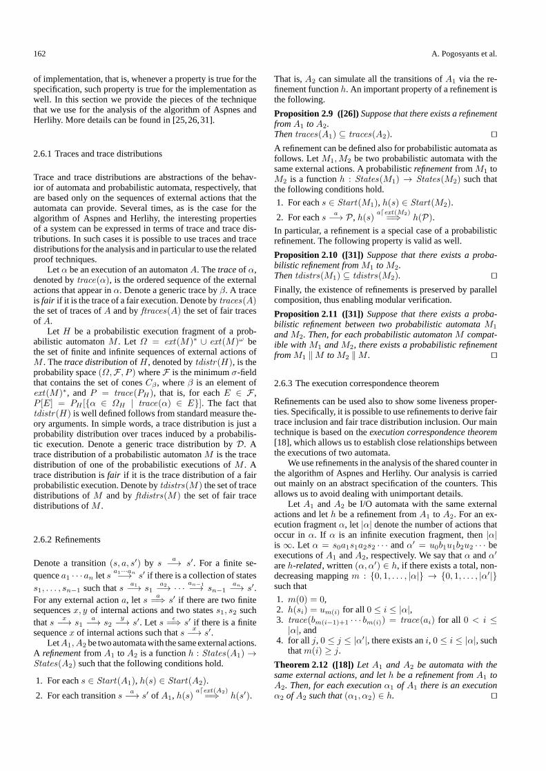
Fig. 2. Interaction diagram of the algorithm of Aspnes and Herlihy
After receiving the initial value to agree on, each processi executes the following loop. It first reads the(value, round)variables of all other processes in its localmemory.Wesay thatprocessi is aleaderif according to its readings its own roundis greater than or equal to the rounds of all other processes.We also say that a processi observedthat another processjis a leader if according toi’s readings the round ofj is greaterthan or equal to the rounds of all other processes. If processiat roundr discovers that it is a leader, and that according to itsreadings all processes that are at roundsr andr − 1 have thesame value asi, theni breaks out of the loop and decides on itsvalue. Otherwise, if all processes thati observed to be leadershave the same valuev , theni sets its value tov, incrementsits round and proceeds to the next iteration of the loop. Inthe remaining case (leaders thati observed do not agree),isets its value to⊥ and scans the other processes again. If onceagain the leaders observed byi do not agree, theni determinesits new preferred value for the next round by invoking a coinflipping protocol. There is a separate coin flipping protocol foreach round. Figure 2 gives a high level view of the algorithm.The left box is the main algorithm which is subdivided intoprocesses; the right boxesare the coin flippingprotocolswhichinteract with the main algorithm through some invocation andresponse messages.
We represent the main part of the algorithm as an automa-tonAP (Agreement Protocol), and the coin flipping protocolsas probabilistic automataCF r (Coin Flipper), one for eachroundr. With this decomposition we can prove several impor-tant properties of the algorithmasproperties ofAP using ordi-nary techniques for non-probabilistic systems. Indeed, in thissection we deal withAP only, and we leave the coin flippersunspecified. Table 1 describes the state variables ofAP . Theshared state of processi consists of a single-writer multiple-reader shared variable with two fields,value(i) andround(i),that contain processi’s current preferred value and round. Thelocal state of a processi consists of a program counterpc, twoarrays,values androunds that store the(value, round) vari-ables of other processes afteri reads them, a variableobs thatrecords the processes already observed byi, a variablestartthat records the initial preferred value ofi, and two booleanflags,decided andstopped , that reflect whetheri has decidedor failed. The variablestopped is not relevant for the actualcode for processi; it is used only in the analysis of the algo-rithm to identify those points where processi has failed.
Table 2 describes the actions and the transition relationof AP . The transitions associated with each actiona are de-scribed by giving the conditions that a states should satisfy toenablea (Pre:), and the transformations that are performed ons to obtain the post-state of the transition (Eff:). If the precon-
dition is omitted, then it is taken to be true. Table 2 is basedon the following predicates and functions:obs-max-round isthe maximum round observed by processi; obs-leader(j) istrue if i observes thatj is a leader;obs-agree(r, v) is true ifthe observations of all the processes whose round is at leastr agree onv; obs-leader-agree(v) is true if, according to theobservations ofi, the leaders agree onv; obs-leader-value isthe value of one of the leaders observed byi. Formally,
obs-max-round = maxj∈obs(rounds[j])
obs-leader(j) = j ∈ obs ∧ rounds[j]= obs-max-round
obs-agree(r, v) = ∀j∈obs rounds[j] ≥ r ⇒ values[j]= v
obs-leader-agree(v) = obs-agree(obs-max-round , v)
obs-leader-value =
vif obs-leader-agree(v)
undefinedif ∃vobs-leader-agree(v)
It is simple to check thatobs-leader-value is a well definedfunction since it is never the case thatobs-leader-agree(0)andobs-leader-agree(1) are satisfied simultaneously.
We associate all the locally controlled actions of a processi with a single task. Thus, an execution fragmentα of AP isfair if all processes that are continuously enabledare scheduledeventually inα.
4.3 Informal analysis of the algorithm
It is easy to show that the algorithmsatisfies validity since if allprocesses start all with the same valuev, then no process willever observe disagreement among the leaders and no processwill ever propose a value different fromv.
It is more difficult to show that the algorithm satisfiesagreement. The first important observation is that agreementdoes not rely on probability, but rather on the fact that theprocesses at the two highest rounds all agree when a processdecides. The very strict condition on the decision action en-sures that no process will ever be able to compromise a de-cision that was taken already. If a process decidesv at roundr, then all processes at roundr agree onv and no process atroundr− 1 can observe leaders with values different fromv.More precisely, suppose for the sake of contradiction that thedecision is taken by processP and that there is a processQat roundr − 1 that is up to proposing a value different fromv for roundr or up to flipping a coin for the value to proposeat roundr. LetQ be the first such process. This means that allprocesses at roundr or higher agree onv. We distinguish twoexhaustive cases.
1. ProcessQ observed that the leaders agree on a value dif-ferent fromv.In this case, since all processes at roundr preferv, processQ observed that the leaders are at roundr−1. Thus, sinceQ is at roundr− 1,Q itself prefers a value different fromv at roundr − 1. Consider the last observation thatPmade ofQ. If P observedQ at roundr−1, then the valuepreferred byQ at roundr − 1 must bev, a contradiction(it is possible to show that a process cannot switch its

168 A. Pogosyants et al.
Table 1.The state variables of a processi in AP
Name Values Initially
Local statepc nil , init , read1, read2, check1, check2,flip,wait , decide initvalues array [1 . . . n] of 0, 1,⊥ array of⊥rounds array [1 . . . n] of int array of0obs set of1, . . . , n ∅start 0, 1,⊥ ⊥decided Bool falsestopped Bool false
Single-writer multiple-reader shared variables(value(i), round(i)) 0, 1,⊥ × int (⊥, 0)
Table 2.The actions and transition relation ofAP
Actions and transitions of processi.
input init(v)i
Eff: start ← v
output start(v)i
Pre: pc = init ∧ start = v = ⊥Eff: value(i)← v
round(i)← 1obs← ∅pc ← read1
output read1(k)i
Pre: pc = read1k /∈ obs
Eff: values[k]← value(k)rounds[k]← round(k)obs← obs ∪ kif obs = 1, . . . , n thenpc ← check1
output check1i
Pre: pc = check1Eff: if obs-leader(i)∧
∃v∈0,1obs-agree(rounds[i]− 1, v) thenpc ← decide
elseif∃v∈0,1obs-leader-agree(v) thenvalue(i)← obs-leader-valueround(i)← rounds[i] + 1obs← ∅pc ← read1
elsevalue(i)← ⊥obs← ∅pc ← read2
output decide(v)i
Pre: pc = decide ∧ values[i] = vEff: decided ← true
pc ← nil
output read2(k)i
Pre: pc = read2k /∈ obs
Eff: values[k]← value(k)rounds[k]← round(k)obs← obs ∪ kif obs = 1, . . . , n thenpc ← check2
output check2i
Pre: pc = check2Eff: if ∃v∈0,1obs-leader-agree(v) then
value(i)← obs-leader-valueround(i)← rounds[i] + 1obs← ∅pc ← read1
elsepc ← flip
output start-flip(r)i
Pre: pc = flipround(i) = r
Eff: pc ← wait
input return-flip(v, r)i
Eff: if pc = wait andround(i) = r thenvalue(i)← vround(i)← rounds[i] + 1obs← ∅pc ← read1
input stopi
Eff: stopped ← truepc ← nil
Tasks:The locally controlled actions of processi form a single task.

Verification of the randomized consensus algorithm of Aspnes and Herlihy: a case study 169
preferred value within a round); ifP did not observeQat roundr − 1, thenP was already at roundr whenQmoved to roundr − 1, which means thatQ observed atleast one process at roundr during its last scan, again acontradiction.
2. ProcessQ observed that the leaders do not agree onv.Since during the second scan of processQ the value pro-posed byQ is⊥, processP observedQ either at a roundlower thanr − 1 or while processQ was scanning theother processes for the first time. In both cases during thesecond scan of roundr− 1 processQ sees that processPis at roundr, and thus that all leaders agree onv. This is acontradiction.
The agreement property is quite intricate to analyze, and theanalysis above may look incomplete since each statement re-lies on the understanding of several subtle interactions be-tween processes. However, assuming that all the statementsare correct, the informal analysis above provides the mainideas behind the correctness of the algorithm of Aspnes andHerlihy. In the formal proof all the informal analysis above isembedded in Invariant 6.3.Weencourage the reader to observecarefully Invariant 6.3 and check how the informal analysisabove is embedded.
The termination property (eventually some process willdecide) relies strongly on the properties of the coin flippingprotocol. If at a certain round the coin flip protocol behaveslike a global coin flip, i.e., like the flip of a unique coin theresult of which is returned to each process, then terminationoccurs within a few rounds. Informally, all the processes thatdo not flip coins to select the value for the next round willselect the same value, and all the processes that flip obtain thesame value. The key problem is how to define a coin flipperthat behaves like a global coin flipper with high probability.We postpone the discussion to Sect. 9.
In the next three sections we prove validity, agreement,and those parts of termination (progress) that do not dependon the low level details of the coin flippers.
5 Proving validity
The proof of validity is very simple and is based on an invari-ant property (cf. Invariant 5.2). In this section and in the restof this paper we use the word “invariant” both for automataand for execution fragments. An invariant of an automaton isa property that is valid in all the reachable states of the au-tomaton; an invariant of an execution fragment is a propertythat is valid in all the states of the execution fragment. Fornotational convenience, givenv ∈ 0, 1, we denote byv thevalue(v + 1)mod 2. We also define a new predicate:agree(r, v) = ∀j(round(j) ≥ r ⇒ value(j) = v).
That is, predicateagree(r, v) is true if all the processes atround at leastr agree on valuev.
Invariant 5.1 Letα be an execution ofAP where no actionof the forminit(v)i occurs. Then each state ofα satisfiesagree(1, v) andobs-agree(1, v).Proof. Straightforward inductive argument. Informally, eachprocess observes that the leaders agree onv, and thus no pro-
cess ever flips a coin or choosesv as its preferred value for thenext round. Invariant 5.2 For each reachable state ofAP , and each pairof processesi, j,
1. s.round(i) = 0 ⇒ s.value(i) = ⊥, and2. s.rounds[i]j = 0 ⇒ s.values[i]j = ⊥.Proof. Straightforward inductive argument.
Theorem 5.3 (Validity property) Let α be an execution ofAP where no action of the forminit(v)i occurs. Then inα noaction of the formdecide(v)i occurs.
Proof. Suppose by contradiction that there is an occurrenceof actiondecide(v)i in α, and lets be the state immediatelybefore actiondecide(v)i. From the transition relation ofAP ,s.values[i]i = v, and by Invariant 5.2,s.rounds[i]i > 0. Thiscontradicts Invariant 5.1.
6 Proving agreement
In this section we prove the agreement property ofAP , that is,that any two processes that decide within an execution decidethe same value (cf. Theorem 6.2).We give the high level proofin Sect. 6.1 and we prove the main invariant in Sect. 6.2.
6.1 High level proof
The key idea of the agreement proof is that if a processi thatis at roundr is “about to decide” on some valuev, then everyprocess that is at roundr or higher has its value equal tov. Weformalize this statement in Invariant 6.1.
Invariant 6.1 Let i be a process. Given a reachable state ofAP , let v = value(i) andr = round(i). Then(obs-agree(r − 1, v)i ∧ obs-leader(i)i ∧ obsi
= 1, . . . , n) ⇒ agree(r, v).
Invariant 6.1 states that if processi has observed all the otherprocesses and has determined that it is a leader and that all theprocesses at round at leastr−1 agree on a valuev, then all theprocesses at round at leastr agree on a valuev. Before givingthe proof of Invariant 6.1, we use Invariant 6.1 to prove theagreement property. Essentially the idea is that the premiseof Invariant 6.1 is stable, that is, it is always satisfied in thefuture once it is satisfied: if processi satisfies the premise ofInvariant 6.1, then processi decides on valuev, and thus thelocal state of processi does not change any more.
Theorem 6.2 (Agreement property)For every traceγ ofAP the following is true: ifdecide(v)i anddecide(v′)j bothoccur inγ thenv = v′.
Proof. Let γ be a trace ofAP such thatdecide(v)i anddecide(v′)j both occur inγ. Letα be an execution ofAP thathas traceγ. Assumewithout loss of generality thatdecide(v)i
occurs first inγ. Let si andsj be the states before actionsdecide(v)i anddecide(v′)j occur, respectively. From the tran-sition relation ofAP , processi satisfies the premise of In-variant 6.1 in statesi, and processj satisfies the premise

170 A. Pogosyants et al.
of Invariant 6.1 in statesj . Thus,si.agree(round(i), v) andsj .agree(round(j), v′). Furthermore, it is a simple inductiveargument to show that the premise of Invariant 6.1 is stable,that is, once it is satisfied it continues to be satisfied. Thus,sj .agree(round(i), v). Since insj there is at least one pro-cess at roundmax (sj .round(i), sj .round(j)), we derive thatv = v′.
6.2 Proof of Invariant 6.1
The problem with Invariant 6.1 is that it is not strong enoughto hold inductively. Therefore, we provide a stronger invariantthat implies Invariant 6.1 and holds inductively. Invariant 6.1guarantees that some properties hold for those states where aprocessi has observed all other processes; for the inductiveargument we need to guarantee some properties also for thosestates where processi has not observed all other processesyet. Furthermore, we need to ensure more properties than justthe fact that all processes at round at leastr have valuev. Inparticular, we need to make sure that all processes at roundr − 1 cannot reach roundr with a value different fromv.
Givenv ∈ 0, 1, denote byv the value(v+1)mod 2. De-fine new predicates and functionsfill-max-round i,fill-leader(j)i,fill-agree(r, v)i, andfill-leader-agree(v)i to be the sameas the corresponding predicates and functionsobs-max -round i, obs-leader(j)i, obs-agree(r, v)i, and obs-leader -agree (v)i, with the following exception: the rounds and pre-ferred values used in the definitions are the values observedby i for the processes thati has already observed, and the ac-tual values of the shared variables for the processes thati hasnot yet observed. In other words, an incomplete observationis “completed instantly” with the actual values of the unob-served processes. Formally, for each processi, letfill-roundsi
andfill-valuesi be two vectors defined as follows:
fill-rounds[j]i=rounds[j]i if j ∈ obsi,round(j) if j /∈ obsi,
fill-values[j]i=values[j]i if j ∈ obsi,value(j) if j /∈ obsi.
The vectorsfill-rounds andfill-values are called thefilledvectors of rounds and values. Then,
fill-max-round i= maxj(fill-rounds[j]i),
fill-leader(j)i= fill-rounds[j]i = fill-max-round i,
fill-agree(r, v)i= fill-roundsi[j]≥ r ⇒ fill-values[j]i = v,
fill-leader-agree(v)i= fill-agree(fill-max-round i, v)i.
The actual invariant that we prove is the following.
Invariant 6.3 Let i be a process. Given a reachable state ofAP , let v = value(i), r = round(i). If the following holds
1. obs-agree(r − 1, v)i,2. fill-agree(r, v)i,3. fill-max-round i = r,
then
a. ∀jobs-agree(r, v)j ,b. agree(r, v),
c. ∀j∈obsi((round(j) = r − 1 ∧ value(j) = v)⇒ fill-max-round j ≥ r).
Informally, Invariant 6.3 states that if nothing is preventingsome processi from deciding on a valuev at roundr, thennone of the processes observed byi is in a position to causeother processes not to agree onv at roundr. Thus, the premisesstate that according to the observations of processi, processi is a leader at roundr and observes that the other processesthat are at round at leastr − 1 agree onv; furthermore all thenon-observed processes do not compromise the leadership ofprocessi and agree onv if they are at round at leastr. Thismeans that it is possible fori to decide onv after completingits scan: the non-observed processes that are at roundr − 1and do not agree onv may reach roundr with valuev beforebeing observed byi. Conditiona states that all processes ob-serve agreement onv from roundr, Conditionb states that allprocesses at round at leastr do agree onv, and Conditioncstates that none of the processes that have been observed al-ready by processi is in a condition to reach roundr with avalue different fromv.
At this point we can understand better the use of⊥ inAP . When a processi is about to decide onv at roundr,it could be the case that another processj at roundr − 1is about to flip a coin for the value to be used in roundr.Processj could have observed some old values of the otherprocesses. However, in such a case the value of processjwould be⊥. Then, Condition c ensure that processj observessome process at round at leastr, and thus, from Condition a,processj observes that the leaders agree onv. Hence, processj cannot flip. In other words, a processj might not discoverthat another processi is about to decide onv at roundr duringits first scan; however, processj would certainly discover theintent of processi during its second scan.
Observe that Invariant 6.3 implies Invariant 6.1 directly;thus, proving Invariant 6.3 is sufficient to prove Invariant 6.1.To prove Invariant 6.3we need several auxiliary invariants thatillustrate some of the key ideas behind the algorithm. Severalinvariants have straightforward inductive proofs, which weomit. The first invariant, Invariant 6.4, states that a processthat has not started yet is at round0.
Invariant 6.4 Let i be a process. Then, for each reachablestate ofAP ,(pci = init) ⇒ (round(i) = 0).
Invariant 6.5 states that a process has observed all other pro-cesseswhenever either it hasdecided, or it is checking the localvariables, or it is interacting with the coin flipping protocol.
Invariant 6.5 Let i be a process. Then, for each reachablestate ofAP ,pci ∈ check1, check2, decide,flip,wait ⇒ obsi
= 1, . . . , n. Invariant 6.6 states that the preferred value of a process is⊥during the second scan of the shared variables and during theinteraction with the coin flipping protocol.
Invariant 6.6 Let i be a process. Then, for each reachablestate ofAP ,pci ∈ read2, check2,flip,wait ⇒ value(i) = ⊥.
Verification of the randomized consensus algorithm of Aspnes and Herlihy: a case study 171
Invariant 6.7 states that if a process is interacting with a coinflipping protocol, then that process observes that the leadersdo not agree.
Invariant 6.7 Let i be a process. Then, for each reachablestate ofAP ,pci ∈ flip,wait ⇒ ∃vobs-leader-agree(v)i.
Invariant 6.8 states that the round numbers observed by eachprocess are never larger than the actual round numbers of theprocesses.
Invariant 6.8 Leti, j be two processes. Then, for each reach-able state ofAP ,rounds[j]i ≤ round(j). Invariant 6.9 is a consequence of the fact that a process cannotprefer two different values during the same round. That is, ifprocessj observes the current round of processi and processidoes not prefer⊥, then then the value of processi observed byprocessj coincides with the actual preferred value of processi. In other words, if processj observes that at some pointprocessi is at roundr and prefers valuev, then the actualpreferred value of processi while its round isr is eitherv or⊥.Invariant 6.9 Leti, j be two processes. Then, for each reach-able state ofAP ,(rounds[i]j = round(i) ∧ value(i) ∈ 0, 1)
⇒ (values[i]j = value(i)).
Proof. For notational convenience, letI(s) denote the invari-ant above. We proveI(s) by induction on the length of anexecution ofAP leading tos. If s is a start state, thenI(s) issatisfied trivially sinces.value(i) = ⊥ for all i. For the induc-tive step it is enough to show that for every transition(s, a, s′)ofAP , I(s) impliesI(s′). We distinguish the following casesbased ona.
1. a = read1(i)j or a = read2(i)j .
The transition relation ofAP ensures thats′.values[i]j =s′.value(i). Thus,I(s′) is true.
2. a = check1i or a = check2i or a = start(v)i, or a =return-flip(v, r)i, v ∈ 0, 1, r > 0.If s′.pci = decide, then none of the relevant variablesfor I(s′) has changed, and thusI(s′) is true; if s′.pci =decide, then eithers′.round(i) = s.round(i) + 1 ors′.value(i) = ⊥ (cf. Ivariants 6.4 and 6.6). In the firstcase, since processj does not change state, and since byInvariant 6.8s.round(i) ≥ s.rounds[i]j , we derive thats′.round(i) > s′.rounds[i]j . Thus, in both cases one ofthe premises ofI(s′) is not satisfied, which means thatI(s′) is true.
3. None of the previous cases hold.
I(s) impliesI(s′) trivially, since all the relevant compo-nents stay unchanged.
Invariant 6.10 states that whenever a process has observeditself, the observed round and value coincide with the actualround and value.
Invariant 6.10 Let i be a process. Then, for each reachablestate ofAP ,i ∈ obsi ⇒ (rounds[i]i =round(i) ∧ values[i]i =value(i)).
Proof. Fix a processi. For notational convenience letI(s)denote the invariant above. We proveI(s) by induction on thelength of an execution ofAP leading tos. If s is a start state,thenI(s) is satisfied trivially sinces.obsi = ∅. For the induc-tive step it is enough to show that for every transition(s, a, s′)ofAP , I(s) impliesI(s′). We distinguish the following casesbased ona.
1. a = read1(i)i or a = read2(i)i.
The transition forread(i)i ensures thats′.rounds[i]i =s.round(i) and thats′.values[i]i = s.value(i). Sinceround(i) andvalue(i) do not change froms to s′, I(s′)is true.
2. a = check1i or a = check2i or a = init(v)i, or a =return-flip(v, r)i, v ∈ 0, 1, r > 0.If s′.pci ∈ decide,flip, then none of the relevant vari-ables forI(s′) has changed froms to s′, andI(s′) is true.If s′.pci /∈ decide,flip, then s′.obs = ∅, falsifyingi ∈ s.obsi. Therefore,I(s′) is satisfied trivially.
3. None of the cases above hold.
I(s) impliesI(s′) trivially, sinceall the relevant conditionsstay unchanged.
Invariant 6.11 states that whenever the maximum round is atmostr and all processes agree on a valuev from roundr, thenall processes observe that there is agreement onv from roundr.
Invariant 6.11 Letrbeanon-negative integerandv ∈ 0, 1.Then, for each reachable state ofAP ,(max-round ≤ r ∧ agree(r, v)) ⇒ ∀jobs-agree(r, v)j .
Proof. Suppose that the premises of the invariant above aresatisfied, and leti, j be two processes such thatrounds[i]j =r. By Invariant 6.8 and frommax-round ≤ r, round(i) =r. Thus, fromagree(r, v), value(i) = v. By Invariant 6.9,values[i]j = v. The following lemma is more technical and is used to shortenthe inductive argument in the proof of Invariant 6.3. It statesthat, under certain conditions, if the premises of Invariant 6.3are satisfied in the post-state of a transition, then the premisesof Invariant 6.3 are satisfied in the pre-state of the transitionas well.
Lemma 6.12 Let (s, a, s′) be a transition ofAP , whereais eitherread1(k)j or read2(k)j or check1j or check2j orreturn-flip(v′, r′)i, v′ ∈ 0, 1, r′ > 0. Let i be a processsuch thati = j if a = check1j or a = check2j or a =return-flip(v′, r′)j . If, for v ∈ 0, 1andr > 0, the followingconditions hold ins′:
1. obs-agree(r − 1, v)i,2. fill-agree(r, v)i,3. fill-max-round i = r,4. value(i) = v andround(i) = r,
then the same conditions hold ins as well.
Proof. We distinguish two cases based ona.
1. a = read1(k)j or a = read2(k)j .
Observe that for each processl, s.value(l) = s′.value(l)ands.round(l) = s′.round(l). This implies Condition4in s. It is left to show Conditions1, 2, and 3 fors. If

172 A. Pogosyants et al.
i = j then s.valuesi = s′.valuesi and s.roundsi =s′.roundsi. Thus, Conditions1, 2, and 3 are satisfied triv-ially in s. If i = j, then for every processl such thatl = k, s.values[l]i = s′.values[l]i ands.rounds[l]i =s′.rounds[l]i. Sincek ∈ s.obsi (i is reading fromk), andsince Condition1 holds ins′, Condition 1 also holds ins.Condition 2 follows directly from Condition 2 fors′ andthe fact thats′.values[k]i = s.value(k) ands′.rounds[k]i= s.round(k); Condition 3 follows from Condition 3 ins′ and froms′.rounds[k]i = s.round(k).
2. a = check1j or a = check2j or a = return-flip(v′, r′)j .
Observe that, by Invariants 6.5 and 6.10,s.round(j) =s.rounds[j]j . Conditions3 and4 are trivial, since the stateof processi is the same ins ands′ (i = j), s.round(j) ≤s′.round(j), ands.round(i) = r. Similarly, Condition1holds ins. It is left to show that Condition 2 holds ins.Sincej is the only process that changes state, and sinceCondition 2 is affected only ifj ∈ s′.obsi, which is equiv-alent toj ∈ s.obsi, it is sufficient to verifys.round(j) =r ⇒ s.value(j) = v under theassumption thatj ∈ s.obsi.We distinguish two cases.(a) s′.pcj ∈ decide,flip.
No other state variable has changed in the transition.Thus, Condition2 holds ins.
(b) s′.pcj = read .
From Condition 3 ins′ we haves′.round(j) ≤ r.If s′.value(j) = ⊥, then Condition2 for s′ impliess′.round(j) < r, and therefores.round(j) < r,which implies Condition2 for s. If s′.value(j) = ⊥,then the transition relation ofAP impliess.round(j)< s′.round(j), and therefore, since from Condition 3s′.round(j) ≤ r, s.round(j) < r. This implies Con-dition 2 for s.
Proof of Invariant 6.3.For notational convenience, for eachstates and processi let I(s) denote the whole invariant,C1 (s, i),C2 (s, i),andC3 (s, i)denoteConditions 1, 2, and3,respectively, andCa(s, i),Cb(s, i), andCc(s, i) denote Con-ditionsa, b, andc, respectively.
We proveI(s) by induction on the length of an executionof AP leading tos. If s is a start state, thenI(s) is satisfiedtrivially sinces.value(j) = ⊥ for all j ands.obsi = ∅, andthusC2 (s, i) is not satisfied. For the inductive step it is enoughto show that for every transition(s, a, s′) ofAP , I(s) impliesI(s′). We distinguish the following cases based ona.
1. a = start(v′)j for somev′ andj.Consider a processesi such thatC1 (s′, i) ∧ C2 (s′, i) ∧C3 (s′, i). Let r = s′.round(i), v = s′.round(i). Wedistinguish the following cases.(a) i = j.
In this caser = 1 andv′ = v. Sinces′.obsi = ∅,Cc(s′, i) is trivially true, andCb(s′, i) follows fromC2 (s′, i). Furthermore, fromC3 (s′, i),s′.max-round= 1, and thus the premises of Invariant 6.11 are satis-fied, givingCa(s′, i).
(b) i = j andr = 1.FromC1 (s′, i),j /∈ s′.obsi, otherwiseprocessiwouldhave observed⊥ at roundr−1. Thus, fromC2 (s′, i),v′ = v. Since, except for processj, all the relevant
components forC1 (s, i) andC2 (s, i) do not change,we deriveC1 (s, i) ∧ C2 (s, i). If C3 (s, i) is true aswell, thenCa(s, i) ∧ Cb(s, i) ∧ Cc(s, i) is true, andCa(s′, i) ∧ Cb(s′, i) ∧ Cc(s′, i) follow directly. IfC3 (s, i) is false, thens.obsi = ∅, otherwiseC1 (s, i)would be false, and thusj is the only process ins′ thatis at roundr. This impliesCb(s′, i)∧Cc(s′, i)directly.By Invariant 6.8,Ca(s, i) is true, and thus, since noneof the relevant state components change,Ca(s′, i) istrue as well.
(c) i = j andr = 2.Observe thatC1 (s, i) ∧ C2 (s, i) ∧ C3 (s, i) is true,since processj does not affect their validity. Thus,Ca(s, i)∧Cb(s, i)∧Cc(s, i) is true. Then,Ca(s′, i)∧Cb(s′, i) since processj does not affect their valid-ity. Sinces′.obsj = ∅, from C3 (s′, i) and by Invari-ant 6.8 we derive that processj satisfies the conditionfor Cc(s′, i). Thus,Cc(s′, i) follows fromCc(s, i).
(d) i = j andr > 2.I(s′) follows trivially from I(s) since processj doesnot affect any of the relevant conditions.
2. a = read1(k)j or a = read2(k)j for somej andk.
Consider a processesi such thatC1 (s′, i) ∧ C2 (s′, i) ∧C3 (s′, i). Let r = s′.round(i), v = s′.round(i). ByLemma 6.12,s.value(i) = v, s.round(i) = r, andC1 (s, i) ∧ C2 (s, i) ∧ C3 (s, i). SinceI(s) is true, wealso haveCa(s, i)∧Cb(s, i)∧Cc(s, i). We need to showCa(s′, i) ∧ Cb(s′, i) ∧ Cc(s′, i).To showCa(s′, i) it is enough to show thats′.rounds[k]j≥ r ⇒ s′.values[k]j = v. From the transition relationof AP , s′.rounds[k]j = s.round(k) ands′.values[k]j =s.value(k). Thus,Cb(s, i) suffices.Cb(s′, i) follows trivially from Cb(s, i) since none of therelevant state components change.
ForCc(s′, i), suppose thatj ∈ s′.obsi,s′.round(j) = r−1,s′.value(j) = v.Observe thati = j sinces.round(i) =r and thuss′.round(i) = r − 1. The termss.fill -max -round j ands′.fill-max-round j differ only in the use ofround(k) androunds[k]j . The transition relation ofAPensures theequalityof the two termsabove.Thus,Cc(s′, i)follows fromCc(s, i).
3. For somej, a = check1j or a = check2j or a = return-flip(v′, r′)i, v′ ∈ 0, 1, r′ > 0.Consider a processesi such thatC1 (s′, i) ∧ C2 (s′, i) ∧C3 (s′, i). Letr = s′.round(i),v = s′.round(i). Observethat, by Invariants 6.5 and 6.10,s.round(j) = s.rounds[j]j . Furthermore, observe that for all processesl,
s′.rounds l = s.rounds l ∧ s′.values l
= s.values l ∧ s′.obsl ⊆ s.obsl. (14)
If s′.pcj ∈ decide,flip, thenI(s′) follows trivially fromI(s) since none of the relevant state components change.Thus, we consider only the case wheres′.pcj = decide.In particular,s′.obsj = ∅.If i = j (ands′.pci /∈ decide,flip), then froms′.obsi =∅wegetCc(s′, i). Furthermore,s′.obsi = ∅ andC2 (s′, i)imply s′.agree(r, v), and thusCb(s′, i) is true. Froms′.obsi = ∅ andC3 (s′, i), we derives′.max-round ≤ r.

Verification of the randomized consensus algorithm of Aspnes and Herlihy: a case study 173
This means that the conditions of Invariant 6.11 are satis-fied, and thusCa(s′, i) is true.If i = j (ands′.pci /∈ decide,flip), then Lemma 6.12implies thats.value(i) = v and s.round(i) = r andC1 (s, i)∧C2 (s, i)∧C3 (s, i). SinceI(s) is true, we haveCa(s, i)∧Cb(s, i)∧Cc(s, i). Equation (14) andCa(s, i)implyCa(s′, i). Sinces′.round(i) = r, froms′.obsj = ∅we derives′.fill-max-round j ≥ r, and thusCc(s′, i) fol-lows fromCc(s, i). To showCb(s′, i) we distinguish thefollowing cases.(a) s.round(j) ≥ r.
By Invariant 6.5,s.obsj = 1, . . . , n, and thus, by In-variant 6.10, s.rounds[j]j = s.round(j). FromCa (s, i), since s.obsj = 1, . . . , n, and sinces.round(j) ≥ r, we derives.obs-leader-agree(v)j .By Invariant6.7,s.pcj = wait , and thus, from the tran-sition relationofAP ,s′.value(j) = v ands′.round(j)> r. Therefore,Cb(s′, i) follows fromCb(s, i).
(b) s.round(j) = r − 1 ands.value(j) = ⊥.By Invariant 6.5,s.obsj = 1, . . . , n. If j ∈ s′.obsi,thenCa(s, i) ∧ Cc(s, i) implies s.obs-leader-agree(v)j . By Invariant 6.7 and from the transition relationof AP , s′.value(j) = v ands′.round(j) = r. There-fore Cb(s′, i) follows from Cb(s, i). If j /∈ s′.obsi,then fromC2 (s′, i), s′.value(j) = v. Thus,Cb(s′, i)follows fromCb(s, i).
(c) s.round(j) = r − 1 ands.value(j) = ⊥.By Invariant 6.5,s.obsj = 1, . . . , n, and by Invari-ant 6.6,a = check1. If j /∈ s′.obsi, thenC2 (s′, i) im-plies ¬s.obs-leader-agree(v)j , since otherwises ′. pre-fer(j)wouldbev; if j ∈ s′.obsi ands.value(j)= v, thenCa(s, i) and Invariant 6.10 imply¬s.obs-leader -agree(v)j ; if j ∈ s′.obsi ands.value(j) = v,then fromCc(s, i) we derives.fill-max-round j ≥ r,and thus, fromCa(s, i), s.obs-leader-agree(v)j .
Thus, in every casewe have¬s.obs-leader-agree(v)j .If s.obs-leader-agree(v)j , then from the transition re-lationofAP wehaves′.value(j) = v ands′.round(j)= r. Therefore,Cb(s′, i) follows from Cb(s, i). If¬s.obs-leader-agree(v)j , then from the transition re-lationofAP wehaves′.value(j)=⊥ands′.round(j)= r − 1. Again,Cb(s′, i) follows fromCb(s, i).
(d) s.round(j) < r − 1.Sinces′.round(j) ≤ r− 1,Cb(s′, i) follows triviallyfromCb(s, i).
4. None of the previous cases hold.
I(s) impliesI(s′) since all the relevant components ofsands′ stay unchanged.
Proof of Invariant 6.1.Follows directly from Invariant 6.3.
7 Non-probabilistic progress properties
Our next objective is to show that in the algorithm of Aspnesand Herlihy some decision is reached within some expectednumber of rounds. This property depends on the probabilisticproperties of the coin flipping protocols. However, there areseveral progress properties of the algorithm that do not depend
on any probabilistic assumption. In this section we study suchproperties. The advantage of this approach is that we can useexisting techniques for ordinary nondeterministic systems andconfine the probabilistic arguments to a very limited section ofthe analysis. In this way we can also point out very preciselywhat is the essential role of probability within the protocolwe analyze. The results of this section are integrated withprobabilistic arguments in Sect. 8.
For each roundr, letCF r be a coin flipping protocol, thatis, a probabilistic automatonwith the interface of a coin flipperofFig. 2.DefineAH (Aspnes-Herlihy) tobeAP‖(‖r≥1CF r).
For each finite execution fragmentα of AH , defineφMaxRound(α) = lstate(α).max-round
−fstate(α).max-round ,wheremax-round is a function that gives themaximum roundnumber among all the processes. Since the round number ofeach process is nondecreasing, it is immediate to verify thatφMaxRound is a complexitymeasure. Define the following setsof states.
R the set of reachable states ofAH such that∃ipci /∈init ,nil;
D the set of reachable states ofAH such that∀i(pci ∈init ,nil).
We call the states ofR active, since they represent situationswhere some process is participating actively in the consensusprotocol.Wewant to show that, under some special conditionson the coin flipping protocols, starting from any state ofR,a state fromD is reached within some bounded number ofrounds. It turns out that it is easier to split the problem in twoparts: firstweshowasimpleproperty that, unless thealgorithmterminates, the system reaches a point where one process hasjustmoved to a newmaximum round (F0 andF1 below,wherethe subscript corresponds to the value preferred by the processat the maximum round); then, we show that from such anintermediate point, under some special conditions on the coinflipping protocols, the algorithm terminates. Formally, definethe following sets of states.
F0 the set of states ofR where there exists a roundr and aprocessl such thatround(l) = r, value(l) = 0, obsl = ∅,and for all processesj = l, round(j) < r;
F1 the set of states ofR where there exists a roundr and aprocessl such thatround(l) = r, value(l) = 1, obsl = ∅,and for all processesj = l, round(j) < r.
We show two properties, the first of which is almost trivial:
1. (Proposition 7.3) IfAH is in a states of R and all in-vocations to the coin flippers on non-failing ports get aresponse, then a state fromF0 ∪F1 ∪D is reached withinone round.
2. (Proposition 7.8) IfAH is in a states ofFv, all invocationsto the coin flippers on non-failing ports get a response, andall invocations toCF s.max-round get only responsev, thena state fromD is reached within two rounds.
To state formally the two properties above we need to definethe meaning of the sentences “all invocations to the coin flip-pers on non-failing ports get responses”, and “all invocationstoCF r get only responsev”, which we identify with the con-cepts ofresponsivenessand(v, r)-globality, respectively.

174 A. Pogosyants et al.
Definition 7.1 Aporti is non-failing inanexecution fragmentα of AH or ofCF r if action stopi does not occur inα.
An invocation toCF r fromprocessi ispendingin a reach-able states of CF r if there is an executionα of CF r, endingin states, such that inα port i is non-failing, there is at leastone occurrence of actionstart-flip(r)i, and the last occur-rence ofstart-flip(r)i is not followed by any action of theform return-flip(v, r)i.
An execution fragmentα of CF r is responsiveif, foreach decompositionα1
α2 of α the following holds: if infstate(α2) there is a pending request of processi toCF r, thenin α2 either actionstopi occurs, or actionreturn-flip(v, r)i
occurs for somev ∈ 0, 1. An execution fragmentα of AHis responsiveif, for eachr > 0, αCF r is responsive.
An execution fragmentα of CF r is v-global iff for eachaction of the formreturn-flip(v′, r)i that occurs inα, v′ = v.An execution fragmentα ofAH is (v, r)-global iff αCF r isv-global. Remark 7.1 The definition of pending request may appearrather cumbersome, since we could state it just in terms of thecomponents of a state ofCF r. The problem is thatCF r is notspecified yet, and thus we cannot refer to its state components:we can refer only to the interactions thatCF r has with itsexternal environment.
Statement 1 is almost trivial and states that within oneround some processmoves first to a new round or all processesterminate. Statement 2 is the key result of this section. It statesthat if the maximum round isr and the process at roundr hasvaluev, then the system quiesces within two rounds ifCF r
behaves like aglobal coinflipper. We start with Statement 1,which requires a trivial preliminary lemma.
Lemma 7.2 Let α be a fair execution fragment ofAH thatstarts from a state ofR, and assume thatα is responsive. Thenin α either a state fromD is reached, ormax-round growsunboundedly.
Proof.Followsdirectly from the fact that all processesperformfinitely many operations in every round. Proposition 7.3 Let s0 be a state ofR, and letα be a fairexecution fragment ofAH that starts from states0. Supposethat α is responsive. Then inα a state ofF0 ∪ F1 ∪ D isreached within one round. That is,α = α1
α2 such thatlstate(α1) ∈ F0 ∪ F1 ∪ D andφMaxRound(α1) ≤ 1.Proof. If D is not reached, then, by Lemma 7.2,max-roundgrows unboundedly. Thus, some process will be the first pro-cess to reach rounds0.max-round + 1. At that point a statefromF0 ∪ F1 is reached. This proves Statement 1. For Statement 2 we need to provesome preliminary invariants. The first invariant is an immedi-ate consequence of the fact that a process has a correct viewof itself whenever it has observed itself.
Invariant 7.4 Let i be a process. Then, for each reachablestate ofAH ,fill-max-round i ≥ round(i).
Proof. Straightforward inductive argument. The second invariant states that the round of each process ismonotonically increasing and that a process cannot prefer bothvalues0 and1 in the same round.
Invariant 7.5 Let α be an execution fragment ofAH , andlet s0 = fstate(α) be reachable inAH . Let l be a process,r = s0.round(l), andv = s0.value(l). If v = ⊥, then foreach state ofα,round(l) ≥ r ∧ (round(l) = r ⇒ value(l) = v).
Proof. Straightforward inductive argument. The third invariant is more technical. The important part isthe second condition, which states that all processes observeagreement on valuev from roundr +1 provided that the coinflipper for roundr always returnsv, that at the beginning thereis exactly one process at roundr, and that the process at roundr prefers valuev. The other two conditions are necessary tocarry out the inductive proof.
Invariant 7.6 Letα be an execution fragment ofAH whosefirst states0 is a state ofFv. Let r = s0.max-round , andlet l be the (unique) process that satisfiess0.round(l) = r.Suppose thatα is (v, r)-global. Then, for each state ofα,
1. ∀j(round(j) = r ⇒ ¬fill-leader-agree(v)j)2. ∀jfill-agree(r + 1, v)j .3. agree(r + 1, v).
Proof. For notational convenience letI(s) denote the wholeinvariant. States0 satisfies Conditions 2 and 3 trivially sinces0.max-round < r + 1. For Condition 1, since processl isthe only process at roundr, and sinces0.value(l) = v ands0.obsl = ∅, it cannot be thecase thats0.fill-leader-agree(v)l.For the inductive step we consider a subsequencesas′ of αand we distinguish cases based ona.
1. a = init(v′)i for somei.
If r > 1, then none of the conditions ofI(s) are affected.If r = 1, then Conditions 2 and 3 are not affected aswell.Consider ageneric processj such thats′.round(j) =r. If j = i, then sinces′.obsj = ∅, Invariant 7.5 andCondition 3 fors′ ensure that¬fill-leader-agree(v)j . Ifj = i, then, since Condition 1 holds ins, there is someprocessk = i that is a leader with value different fromv inthe filled vector of processj. We know thatk = i because,by Invariant 7.4,s.fill-max-round j ≥ r, and thus processi could not affect Condition 1 ins. Thekth entry of thefilled vector ofj is not affected during the transition froms to s′, and thus Condition 1 is preserved.
2. a = read1(k)i or a = read2(k)i for somei andk.
In this case Condition 3 is not affected. Thus, we needto deal only with Conditions 1 and 2, which are affectedonly for processi. In particular, Conditions 1 and 2 dif-fer in s ands′ for the use of(round(k), value(k)) and(rounds[k]i, values[k]i), respectively. The transition re-lation ofAP ensures the equality of the terms above, andthus the preservation of Conditions 1 and 2.
3. a = check1i or a = check2i or a = return-flip(v′, r′)i
for somei.
We consider only the case wherer′ = round(i), sinceotherwise nothing changes during the transition froms tos′. We distinguish the following cases.(a) s.round(i) < r − 1.
In this caseI(s′) follows trivially from I(s) since noneof the conditions are affected.

Verification of the randomized consensus algorithm of Aspnes and Herlihy: a case study 175
(b) s.round(i) = r − 1.Conditions 2 and 3 are not affected. Ifs′.round(i) =r − 1, then Condition 1 is not affected as well. Oth-erwise,s′.obsi = ∅. Observe also thati = l. Thus,Condition 1 follows from Condition 1 fors and byInvariant 7.5.
(c) s.round(i) = r.
If s′.round(i) = r, then Conditions 2 and 3 are notaffected. For Condition 1, ifs′.pci = decide, thenCondition 1 is not affected; otherwise,s′.value(i) =⊥ ands′.obsi = ∅. Thus, Condition 1 follows fromCondition 1 fors and from Condition 3.
If s′.round(i) = r+1, thenCondition 1and the transi-tion relation ofAP(v, r) ensure thats′.value(i) = v.Thus, Conditions 1, 2 and 3 are all preserved.
(d) s.round(i) > r.
From Condition 2 ons, either processi decides onv,or a new round is reached with preferencev. In bothcases Conditions 1, 2 and 3 are preserved.
4. None of the previous cases hold.
I(s′) follows trivially from I(s) since none of the relevantstate components change.
Finally, we can show that fromFv the maximum round of theprocesses does not grow bymore than2 provided that the coinflipper at the maximum round always returnsv.
Invariant 7.7 Letα be an execution fragment ofAH whosefirst states0 is a state ofFv. Letr = s0.max-round . Supposethatα is (v, r)-global. Then, for each state ofα, and for eachprocessj, round(j) ≤ r + 2.
Proof. First observe thatα satisfies the conditions of Invari-ant 7.6, which means that Invariant 7.6 is satisfied by all thestates ofα.
All the cases for the proof are straightforward except forthe case where a transition(s, check1j , s
′) occurs ands.round(j) = r+2. In such case, from Condition 2 of Invari-ant 7.6,s.fill-agree(r + 1, v)j . Sinces.obsj = 1, . . . , n,we derive thats.obs-agree(r + 1, v), and thus processj setspcj to decide without reaching roundr + 3. Observe thatcheck2j cannot occur whenround(j) = r + 2 since in suchcasevalue(j) = ⊥ and Invariant 7.6 would be violated. Proposition 7.8 Let α be a fair execution fragment ofAHwhose first states0 is a state ofFv. Let r = s0.max-round .Suppose thatα is responsive and(v, r)-global. Then inα astate fromD is reachedwithin two rounds.That is,α = α1
α2wherelstate(α1) ∈ D andφMaxRound(α1) ≤ 2.
Proof. Suppose thatD is not reached inα. Then, byLemma 7.2, some process eventually reaches roundr + 3,contradicting Invariant 7.7. Therefore, inα a state fromDis reached. Furthermore, by Invariant 7.7, a state fromD isreached within two rounds.
8 Probabilistic progress properties
Suppose that each coin flipping protocolCF r satisfies thefollowing properties.
C1 For each fair probabilistic execution fragment ofCF r thatstarts with a reachable state ofCF r, the probability of theexecution fragments that are responsive is1.
C2 For each fair probabilistic execution ofCF r, and eachvaluev ∈ 0, 1, the probability of the executions thatare responsive andv-global is at leastp, wherep is a realnumber such that0 < p ≤ 1.
In this section we show that under ConditionsC1 andC2 foreveryCF r,AH guarantees progress within expectedO(1/p)rounds. That is, we prove the following proposition.
Proposition 8.1 If each coin flipping protocolCF r satisfiespropertiesC1 andC2, then inAH , starting from any stateofR and under any fair scheduler, a state fromD is reachedwithin at mostO(1/p) expected rounds.
Thus, we need to show only that it is possible to build dis-tributed implementations of the coin flippers that satisfyC1andC2with a suitable value forp. We build the implementa-tions in Sects. 9 and 10.
Remark 8.1Observe that propertyC1 refers to probabilisticexecution fragments, while PropertyC2 refers to probabilisticexecutions. This distinction is important. PropertyC1 statesthat a coin flipper gives responses with probability1 from anyarbitrary point in its computation; PropertyC2guarantees thatwith probabilityp a specific value is always returned, but onlyif we observe the coin flipper from the beginning.C2 is nottrue for an arbitrary probabilistic execution fragment: if weconsider a fragment that begins in a state where two processesare about to return two different values, then all processesreturn the same value with probability0.
We now turn to the proof of Proposition 8.1. The mainstatement that we use isR φMaxRound≤3−→
pD. (15)
To prove Statement (15) we prove two intermediate state-ments:R φMaxRound≤1−→
1F0 ∪ F1 ∪ D, (16)
and for eachv ∈ 0, 1,Fv
φMaxRound≤2−→p
D. (17)
TheproofsofStatements (16) and (17) rely onPropositions7.3and 7.8 and on the probabilistic properties of the coin flippingprotocols. In particular, the first statement relies on the factthat the coin flippers respond, which occurs with probability 1(C1), and the second statement relies on the fact that somespecific coin flipper always returns a specific valuev, whichis the case with probability at leastp (C2).
Proposition 8.2 Assuming that the coin flippers inAH satisfyC1,
R φMaxRound≤1−→1
F1 ∪ F0 ∪ D. (18)
Proof. Let H be a probabilistic execution fragment ofAHthat starts from a state ofR. LetΘ be the set of executions ofΩH where each invocation to any coin flipper on a non-failingport gets a response. By Proposition 7.3, in each executionof Θ a state fromF1 ∪ F0 ∪ D is reached within one round.Thus, it is sufficient to show thatPH [Θ] = 1. Let, for eachi ≥ 1, Θi be the set of executions ofΩH where each in-vocation toCF i on a non-failing port gets a response. Then
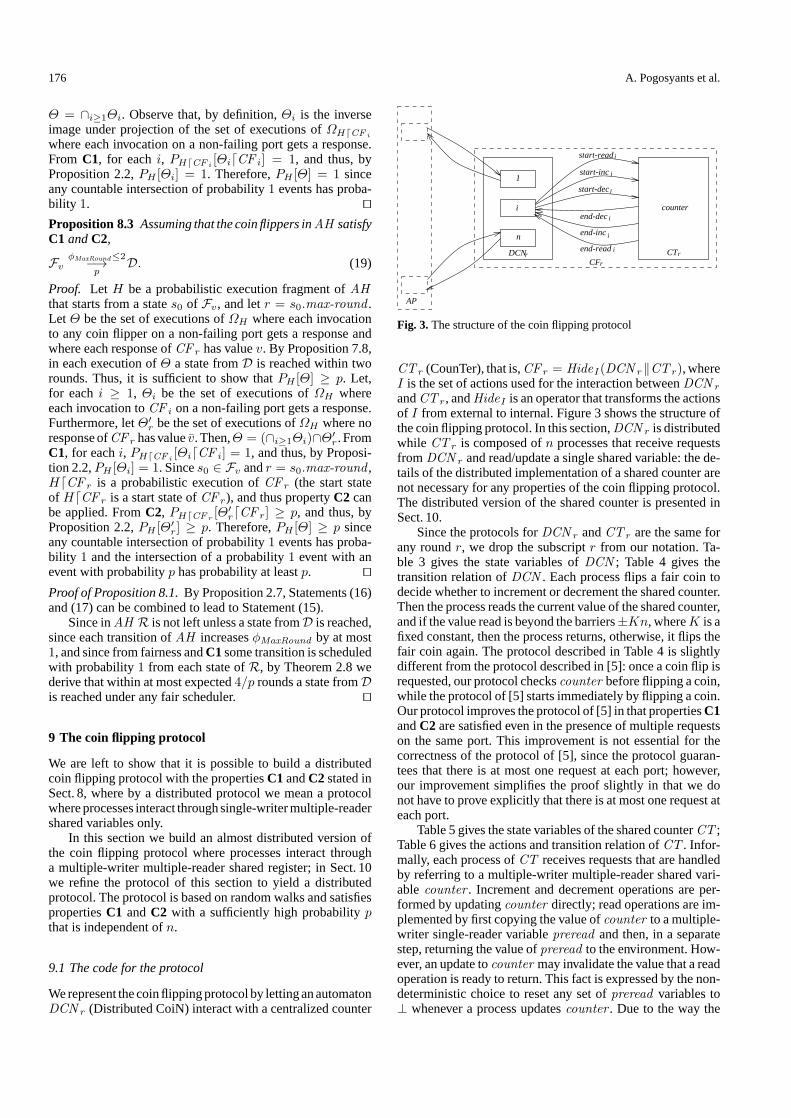
176 A. Pogosyants et al.
Θ = ∩i≥1Θi. Observe that, by definition,Θi is the inverseimage under projection of the set of executions ofΩHCF i
where each invocation on a non-failing port gets a response.From C1, for eachi, PHCF i
[ΘiCF i] = 1, and thus, byProposition 2.2,PH [Θi] = 1. Therefore,PH [Θ] = 1 sinceany countable intersection of probability1 events has proba-bility 1. Proposition 8.3 Assuming that the coin flippers inAH satisfyC1 andC2,
FvφMaxRound≤2−→
pD. (19)
Proof. Let H be a probabilistic execution fragment ofAHthat starts from a states0 of Fv, and letr = s0.max-round .LetΘ be the set of executions ofΩH where each invocationto any coin flipper on a non-failing port gets a response andwhere each response ofCF r has valuev. By Proposition 7.8,in each execution ofΘ a state fromD is reached within tworounds. Thus, it is sufficient to show thatPH [Θ] ≥ p. Let,for eachi ≥ 1, Θi be the set of executions ofΩH whereeach invocation toCF i on a non-failing port gets a response.Furthermore, letΘ′
r be the set of executions ofΩH where noresponseofCF r hasvaluev. Then,Θ = (∩i≥1Θi)∩Θ′
r. FromC1, for eachi, PHCF i
[ΘiCF i] = 1, and thus, by Proposi-tion 2.2,PH [Θi] = 1. Sinces0 ∈ Fv andr = s0.max-round ,HCF r is a probabilistic execution ofCF r (the start stateof HCF r is a start state ofCF r), and thus propertyC2 canbe applied. FromC2, PHCFr
[Θ′rCF r] ≥ p, and thus, by
Proposition 2.2,PH [Θ′r] ≥ p. Therefore,PH [Θ] ≥ p since
any countable intersection of probability1 events has proba-bility 1 and the intersection of a probability1 event with anevent with probabilityp has probability at leastp. Proof of Proposition 8.1.By Proposition 2.7, Statements (16)and (17) can be combined to lead to Statement (15).
Since inAH R is not left unless a state fromD is reached,since each transition ofAH increasesφMaxRound by at most1, and since from fairness andC1some transition is scheduledwith probability1 from each state ofR, by Theorem 2.8 wederive that within at most expected4/p rounds a state fromDis reached under any fair scheduler.
9 The coin flipping protocol
We are left to show that it is possible to build a distributedcoin flipping protocol with the propertiesC1andC2 stated inSect. 8, where by a distributed protocol we mean a protocolwhereprocesses interact throughsingle-writermultiple-readershared variables only.
In this section we build an almost distributed version ofthe coin flipping protocol where processes interact througha multiple-writer multiple-reader shared register; in Sect. 10we refine the protocol of this section to yield a distributedprotocol. The protocol is based on random walks and satisfiespropertiesC1 andC2 with a sufficiently high probabilitypthat is independent ofn.
9.1 The code for the protocol
Werepresent thecoinflippingprotocol by lettinganautomatonDCN r (Distributed CoiN) interact with a centralized counter
CTr
n
1
i
i
i
i
i
i
start-read
start-inc
start-dec
end-dec
end-inc
end-readr
rCF
i counter
DCN
AP
Fig. 3.The structure of the coin flipping protocol
CT r (CounTer), that is,CF r = HideI(DCN r‖CT r), whereI is the set of actions used for the interaction betweenDCN r
andCT r, andHideI is an operator that transforms the actionsof I from external to internal. Figure 3 shows the structure ofthe coin flipping protocol. In this section,DCN r is distributedwhile CT r is composed ofn processes that receive requestsfromDCN r and read/update a single shared variable: the de-tails of the distributed implementation of a shared counter arenot necessary for any properties of the coin flipping protocol.The distributed version of the shared counter is presented inSect. 10.
Since the protocols forDCN r andCT r are the same forany roundr, we drop the subscriptr from our notation. Ta-ble 3 gives the state variables ofDCN ; Table 4 gives thetransition relation ofDCN . Each process flips a fair coin todecide whether to increment or decrement the shared counter.Then the process reads the current value of the shared counter,and if the value read is beyond the barriers±Kn, whereK is afixed constant, then the process returns, otherwise, it flips thefair coin again. The protocol described in Table 4 is slightlydifferent from the protocol described in [5]: once a coin flip isrequested, our protocol checkscounter before flipping a coin,while the protocol of [5] starts immediately by flipping a coin.Our protocol improves the protocol of [5] in that propertiesC1andC2 are satisfied even in the presence of multiple requestson the same port. This improvement is not essential for thecorrectness of the protocol of [5], since the protocol guaran-tees that there is at most one request at each port; however,our improvement simplifies the proof slightly in that we donot have to prove explicitly that there is at most one request ateach port.
Table 5 gives the state variables of the shared counterCT ;Table 6 gives the actions and transition relation ofCT . Infor-mally, each process ofCT receives requests that are handledby referring to a multiple-writer multiple-reader shared vari-ablecounter . Increment and decrement operations are per-formed by updatingcounter directly; read operations are im-plemented by first copying the value ofcounter to a multiple-writer single-reader variablepreread and then, in a separatestep, returning the value ofpreread to the environment. How-ever, an update tocounter may invalidate the value that a readoperation is ready to return. This fact is expressed by the non-deterministic choice to reset any set ofpreread variables to⊥ whenever a process updatescounter . Due to the way the
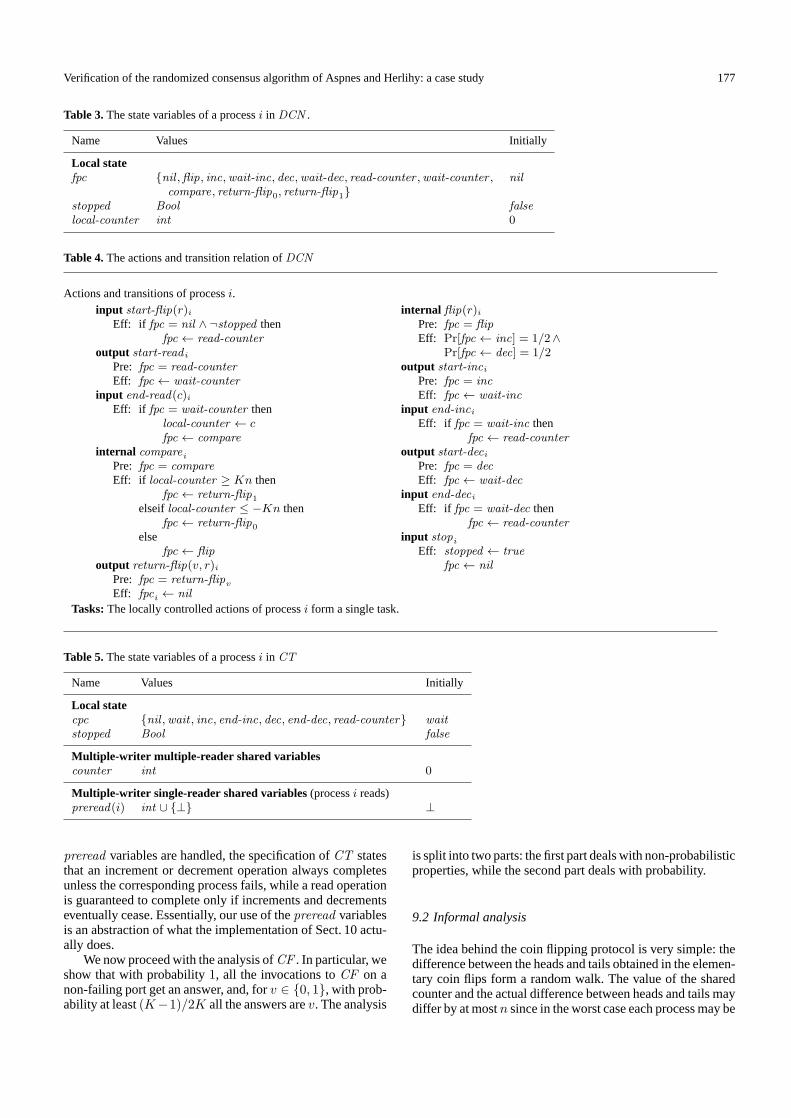
Verification of the randomized consensus algorithm of Aspnes and Herlihy: a case study 177
Table 3.The state variables of a processi in DCN .
Name Values Initially
Local statefpc nil ,flip, inc,wait-inc, dec,wait-dec, read-counter ,wait-counter , nil
compare, return-flip0, return-flip1stopped Bool falselocal-counter int 0
Table 4.The actions and transition relation ofDCN
Actions and transitions of processi.input start-flip(r)i
Eff: if fpc = nil ∧ ¬stopped thenfpc ← read-counter
output start-read i
Pre: fpc = read-counterEff: fpc ← wait-counter
input end-read(c)i
Eff: if fpc = wait-counter thenlocal-counter ← cfpc ← compare
internal comparei
Pre: fpc = compareEff: if local-counter ≥ Kn then
fpc ← return-flip1elseif local-counter ≤ −Kn then
fpc ← return-flip0else
fpc ← flipoutput return-flip(v, r)i
Pre: fpc = return-flipv
Eff: fpci ← nil
internal flip(r)i
Pre: fpc = flipEff: Pr[fpc ← inc] = 1/2∧
Pr[fpc ← dec] = 1/2output start-inci
Pre: fpc = incEff: fpc ← wait-inc
input end-inci
Eff: if fpc = wait-inc thenfpc ← read-counter
output start-deci
Pre: fpc = decEff: fpc ← wait-dec
input end-deci
Eff: if fpc = wait-dec thenfpc ← read-counter
input stopi
Eff: stopped ← truefpc ← nil
Tasks:The locally controlled actions of processi form a single task.
Table 5.The state variables of a processi in CT
Name Values Initially
Local statecpc nil ,wait , inc, end-inc, dec, end-dec, read-counter waitstopped Bool false
Multiple-writer multiple-reader shared variablescounter int 0
Multiple-writer single-reader shared variables (processi reads)preread(i) int ∪ ⊥ ⊥
preread variables are handled, the specification ofCT statesthat an increment or decrement operation always completesunless the corresponding process fails, while a read operationis guaranteed to complete only if increments and decrementseventually cease. Essentially, our use of thepreread variablesis an abstraction of what the implementation of Sect. 10 actu-ally does.
We now proceedwith the analysis ofCF . In particular, weshow that with probability1, all the invocations toCF on anon-failing port get an answer, and, forv ∈ 0, 1, with prob-ability at least(K−1)/2K all the answers arev. The analysis
is split into two parts: the first part dealswith non-probabilisticproperties, while the second part deals with probability.
9.2 Informal analysis
The idea behind the coin flipping protocol is very simple: thedifference between the heads and tails obtained in the elemen-tary coin flips form a random walk. The value of the sharedcounter and the actual difference between heads and tails maydiffer by at mostn since in the worst case each processmay be
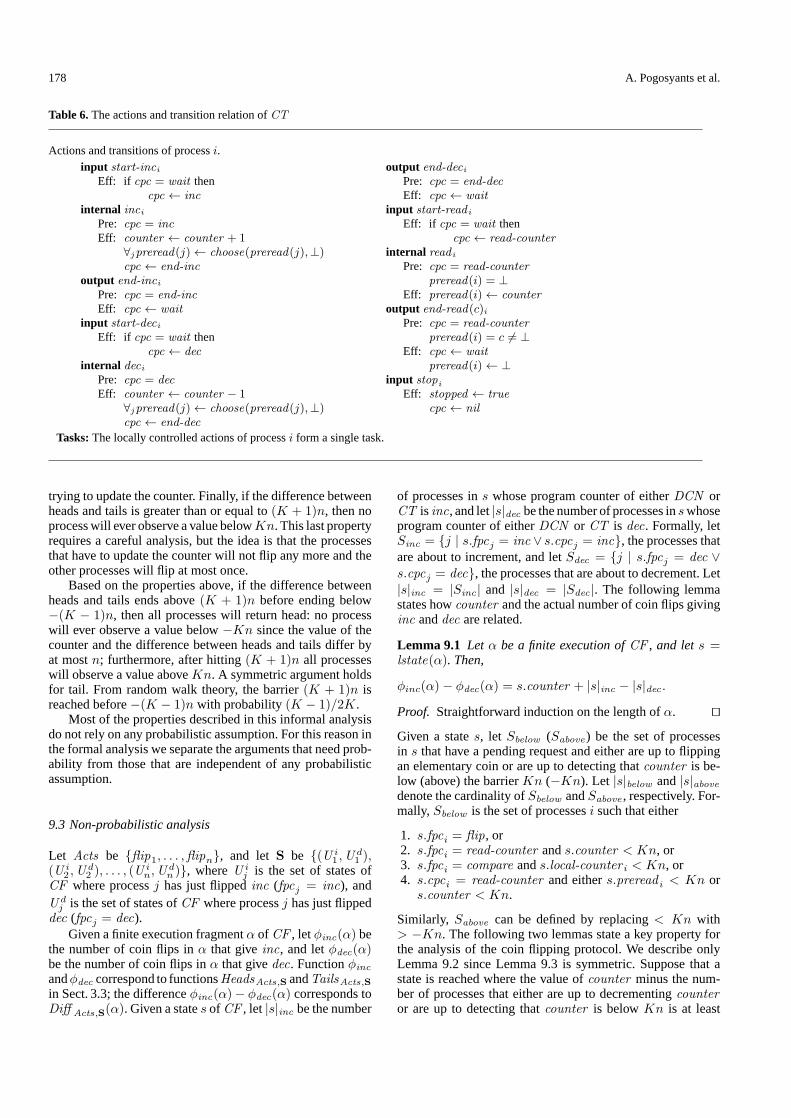
178 A. Pogosyants et al.
Table 6.The actions and transition relation ofCT
Actions and transitions of processi.input start-inci
Eff: if cpc = wait thencpc ← inc
internal inci
Pre: cpc = incEff: counter ← counter + 1
∀jpreread(j)← choose(preread(j),⊥)cpc ← end-inc
output end-inci
Pre: cpc = end-incEff: cpc ← wait
input start-deci
Eff: if cpc = wait thencpc ← dec
internal deci
Pre: cpc = decEff: counter ← counter − 1
∀jpreread(j)← choose(preread(j),⊥)cpc ← end-dec
output end-deci
Pre: cpc = end-decEff: cpc ← wait
input start-read i
Eff: if cpc = wait thencpc ← read-counter
internal read i
Pre: cpc = read-counterpreread(i) = ⊥
Eff: preread(i)← counteroutput end-read(c)i
Pre: cpc = read-counterpreread(i) = c = ⊥
Eff: cpc ← waitpreread(i)← ⊥
input stopi
Eff: stopped ← truecpc ← nil
Tasks:The locally controlled actions of processi form a single task.
trying to update the counter. Finally, if the difference betweenheads and tails is greater than or equal to(K + 1)n, then noprocesswill ever observe a value belowKn. This last propertyrequires a careful analysis, but the idea is that the processesthat have to update the counter will not flip any more and theother processes will flip at most once.
Based on the properties above, if the difference betweenheads and tails ends above(K + 1)n before ending below−(K − 1)n, then all processes will return head: no processwill ever observe a value below−Kn since the value of thecounter and the difference between heads and tails differ byat mostn; furthermore, after hitting(K + 1)n all processeswill observe a value aboveKn. A symmetric argument holdsfor tail. From random walk theory, the barrier(K + 1)n isreached before−(K − 1)n with probability(K − 1)/2K.
Most of the properties described in this informal analysisdo not rely on any probabilistic assumption. For this reason inthe formal analysis we separate the arguments that need prob-ability from those that are independent of any probabilisticassumption.
9.3 Non-probabilistic analysis
Let Acts be flip1, . . . ,flipn, and let S be (U i1 ,U
d1 ),
(U i2 ,U
d2 ), . . . , (U i
n,U dn ), whereU i
j is the set of states ofCF where processj has just flippedinc (fpcj = inc), andU d
j is the set of states ofCF where processj has just flippeddec (fpcj = dec).
Given a finite execution fragmentα ofCF , letφinc(α) bethe number of coin flips inα that giveinc, and letφdec(α)be the number of coin flips inα that givedec. Functionφincandφdec correspond to functionsHeadsActs,S andTailsActs,Sin Sect. 3.3; the differenceφinc(α)− φdec(α) corresponds toDiff Acts,S(α). Given a states ofCF , let |s|inc be the number
of processes ins whose program counter of eitherDCN orCT is inc, and let|s|dec be the number of processes inswhoseprogram counter of eitherDCN or CT is dec. Formally, letSinc = j | s.fpcj = inc ∨ s.cpcj = inc, the processes thatare about to increment, and letSdec = j | s.fpcj = dec ∨s.cpcj = dec, the processes that are about to decrement. Let|s|inc = |Sinc | and |s|dec = |Sdec |. The following lemmastates howcounter and the actual number of coin flips givinginc anddec are related.
Lemma 9.1 Let α be a finite execution ofCF , and lets =lstate(α). Then,
φinc(α)− φdec(α) = s.counter + |s|inc − |s|dec .Proof. Straightforward induction on the length ofα. Given a states, let Sbelow (Sabove ) be the set of processesin s that have a pending request and either are up to flippingan elementary coin or are up to detecting thatcounter is be-low (above) the barrierKn (−Kn). Let |s|below and|s|abovedenote the cardinality ofSbelow andSabove , respectively. For-mally,Sbelow is the set of processesi such that either
1. s.fpci = flip, or2. s.fpci = read-counter ands.counter < Kn, or3. s.fpci = compare ands.local-counter i < Kn, or4. s.cpci = read-counter and eithers.preread i < Kn or
s.counter < Kn.
Similarly, Sabove can be defined by replacing< Kn with> −Kn. The following two lemmas state a key property forthe analysis of the coin flipping protocol. We describe onlyLemma 9.2 since Lemma 9.3 is symmetric. Suppose that astate is reached where the value ofcounter minus the num-ber of processes that either are up to decrementingcounteror are up to detecting thatcounter is belowKn is at least

Verification of the randomized consensus algorithm of Aspnes and Herlihy: a case study 179
Kn. Then Lemma 9.2 states that this property continues to re-main valid in the future. Roughly speaking, each process thatreadscounter terminates (does not flip nor updatecounterany more) because it observes a value that is at leastKn.
Lemma 9.2 The following property is stable forCF , that is,it continues to be satisfied once it is satisfied.
s.counter − |s|dec − |s|below ≥ Kn. (20)
Proof. Straightforward inductive argument. Lemma 9.3 The following property is stable forCF .
s.counter + |s|inc + |s|above ≤ −Kn. (21)
Proof. Straightforward inductive argument. Asimple consequenceof Lemmas9.2and9.3 is thatwhen-
ever the difference between the coin flips that giveinc and thecoin flips that givedec is beyond the barriers±(K + 1)n, thevalue ofcounter is always beyond±Kn.
Lemma 9.4 Let α = α1 α2 be an execution ofCF such
thatφinc(α1)−φdec(α1) = (K +1)n. Then each state ofα2satisfiescounter ≥ Kn.
Proof. By Lemma 9.1,φinc(α1)− φdec(α1) = s.counter +|s|inc − |s|dec wheres = lstate(α1) = fstate(α2), and thuss.counter+|s|inc−|s|dec = (K+1)n. By a simple algebraicmanipulation,s.counter − |s|dec − |s|below = s.counter +|s|inc − |s|dec − (|s|inc + |s|below ). Observe that, by defini-tion,Sinc ∩ Sbelow = ∅, and therefore|s|inc + |s|below ≤ n.This means thats.counter − |s|dec − |s|below ≥ Kn. ByLemma 9.2, each states′ of α2 satisfiess′.counter−|s′|dec−|s′|below ≥ Kn. Thus, each state ofα2 satisfiescounter ≥Kn. Lemma 9.5 Let α = α1
α2 be an execution ofCF suchthatφinc(α1)− φdec(α1) = −(K + 1)n. Then each state ofα2 satisfiescounter ≤ −Kn.
Proof. Symmetric to the proof of Lemma 9.4. Lemma 9.6 Let α be an execution ofCF , such thatα ∈Top[−(K−1)n, (K +1)n, 0](H) for some probabilistic ex-ecutionH ofCF . Thenα is 1-global.
Proof. Sinceα ∈ Top[−(K − 1)n, (K + 1)n, 0](H), ei-ther each prefixα′ of α satisfies−(K − 1)n < φinc(α′) −φdec(α′) < (K + 1)n, or α = α1
α2 whereφinc(α1) −φdec(α1) = (K+1)nandnoprefixα′
1 ofα1 satisfiesφinc(α′1)
−φdec(α′1) ≤ −(K − 1)n.
In the first case, by Lemma 9.1, no state ofα satisfiescounter ≤ −Kn. In the second case, by Lemma 9.1, no stateofα1 satisfiescounter ≤ −Kn. Furthermore, by Lemma9.4,each state ofα2 satisfiescounter ≥ Kn. Therefore, no stateof α satisfiescounter ≤ −Kn. This means that in both casesno process returns value0 in α. Lemma 9.7 Let α be an execution ofCF , such thatα ∈Bottom[−(K−1)n, (K+1)n, 0](H) for someprobabilisticexecutionH ofCF . Thenα is 0-global.
Proof. Symmetric to the proof of Lemma 9.6. Lemma 9.8 Letα be a fair execution ofCF , such thatα ∈Either[−(K + 1)n, (K + 1)n, 0](H) for some probabilisticexecutionH ofCF . Thenα is responsive.
Proof. If α contains finitely many flip actions, then even-tually all the increment and decrement operations derivingfrom the flipping operations are completed or interrupted (thecorrespondingend-inc or end-dec actions occur or the corre-sponding processes fail). Thus, there is a point after which nomoreinc anddec operations are performed. Letα′ be a suffixof α where no more flip, increment or decrement operationsare performed. Then inα′ none of thepreread i variables is setto ⊥ while actionend-read(c)i is enabled, and thus all readoperations on non-failing ports terminate eventually. At thatpoint, since no more flips are performed inα′, each processthat completes a read operation returns a value.
If α contains infinitely many flip actions, then, sinceα ∈Either[−(K + 1)n, (K + 1)n, 0](H), α = α1
α2 suchthatφinc(α1) − φdec(α1) = ±(K + 1)n. Here we considerthe case whereφinc(α1) − φdec(α1) = (K + 1)n; the othercase is symmetric. By Lemma 9.4, each state ofα2 satisfiescounter ≥ Kn. Thus, eachnon-failingprocess returnsavalueonce it readscounter (performing the read operation inα2)since the value read is at leastKn. Lemma 9.9 Letα be a fair execution ofCF , such thatα ∈Top[−(K−1)n, (K +1)n, 0](H) for some probabilistic ex-ecutionH ofCF . Thenα is responsive and1-global.
Proof. By Lemma 9.8, each invocation on a non-failing portgets a response. By Lemma 9.6 no invocation gets response0.Hence, each invocation on a non-failing port gets response1.
Lemma 9.10 Letα be a fair execution ofCF , such thatα ∈Bottom[−(K−1)n, (K+1)n, 0](H) for someprobabilisticexecutionH ofCF . Thenα is responsive and0-global.
Proof. Symmetric to the proof of Lemma 9.9.
9.4 Probabilistic analysis
In this short subsection we prove the probabilistic propertiesof the coin flipping protocol, that is, it guarantees propertiesC1 (Proposition 9.11) andC2 (Proposition 9.12). The proofsrely on the non-probabilistic properties proved in Sect. 9.3 andon the coin lemmas for symmetric random walks of Sect. 3.3.
Proposition 9.11 The coin flipperCF satisfiesC1. That is,for each fair probabilistic execution fragment ofCF that startswith a reachable state ofCF , the probability of the executionsthat are responsive is1.
Proof. Let H be a fair probabilistic execution fragment ofCF that starts with a reachable states of CF , and letαbe a finite execution ofCF such thatlstate(α) = s. Letz = φinc(α) − φdec(α). If α′ is an execution of the eventEither[−(K + 1)n, (K + 1)n, z](H), thenα α′ is an ex-ecution ofEither[−(K − 1)n, (K + 1)n, 0](H ′) for somefair probabilistic executionH ′ ofCF , and by Lemma 9.8, ev-ery invocation toCF in α α′ gets a response. From Defini-tion 7.1, every invocation toCF inα′ gets a response. By The-orem 3.10,PH [Either[−(K + 1)n, (K + 1)n, z](H)] = 1.This completes the proof. Proposition 9.12 The coin flipperCF satisfiesC2 with p =(K + 1)/2K. That is, fixedv ∈ 0, 1, for each fair proba-bilistic execution ofCF , the probability of the executions thatare responsive andv-global is at least(K − 1)/2K.

180 A. Pogosyants et al.
Table 7.The state variables of a processi in DCT
Name Values Initially
Local statecpc nil ,wait , inc, end-inc, dec, end-dec, scan, read-counter waitprescan array [1 . . . n] of int × int array of(0, 0)first array [1 . . . n] of int × int array of(0, 0)obs set of1, . . . , n ∅stopped Bool false
Single-writer multiple-reader shared variables(num(i), val(i)) int × int (0, 0)
Proof.Assume thatv = 1; the case forv = 0 is symmetric. LetH be a fair probabilistic execution ofCF . If α is an executionof Top[−(K − 1)n, (K + 1)n, 0](H), then, by Lemma 9.9,every invocation toCF in α gets response1. Furthermore,by Theorem 3.10,PH [Top[−(K− 1)n, (K +1)n, 0](H)] ≥(K − 1)/2K. This completes the proof.
10 Implementation of the shared counter
In this sectionwebuild an implementation ofCT andweshowthat it can replace the abstract automatonCT in CF withoutcompromising Propositions 9.11 and 9.12, that is, propertiesC1andC2with p = (K− 1)/2K. In this way, using the coinflippingprotocolwith thenewcounter,weobtainaprotocol forconsensus that uses only single-writer multiple-reader sharedvariables.
The implementation ofCT , which we denote byDCT(Distributed CounTer), is an adaptation of an algorithm pro-posed by Lamport [21] for read/write registers. The state vari-ablecounter ofCT is representedbynsingle-writermultiple-reader registers, one for each process, with two fields: anumfield, which is incremented whenever the value of the registeris changed, and aval field representing the contribution of thecorresponding process to the value ofcounter . The operationsinc anddec on a processi are implemented by incrementingor decrementing theval register and incrementing thenumregister of processi. The operationread-counter is imple-mented by scanning the shared registers until two consecutivescans give the same value. Table 7 gives the state variables ofDCT ; Table 8 gives the transition relation ofDCT .
We now verify that it is possible to replaceDCT for CTinCF without compromising propertiesC1andC2. LetDCF(DistributedCoinFlipper) bedefinedasHideI(DCN ‖DCT ),whereI is the set of actions used for the interaction betweenDCN andDCT .
Observe that propertiesC1 andC2 are properties of thefair trace distributions ofCF andDCF . Specifically, observethat responsiveness andv-globality can be stated in terms oftraces. Then, propertyC1 can be stated as “in each fair tracedistribution, the probability of the set of traces that are re-sponsive is 1”, and propertyC2 can be stated as: “in eachfair trace distribution, the probability of the set of traces thatare responsive andv-global is at least p”. Thus, to show thatDCF satisfies propertiesC1andC2 it is sufficient to show thatftdistrs(DCF ) ⊆ ftdistrs(CF ). For this purpose, by usingProposition 2.13, it is sufficient to build a refinementh from
DCT toCT and show thath preserves the fair executions ofDCT . Note thath is not probabilistic sinceDCT andCT arenot probabilistic. That is, the properties that we need to showdo not involve probability.
Proposition 10.1 There is a refinement fromDCT toCT thatpreserves the fair executions ofDCT .
Proof. The refinement keeps thepreread variables differentfrom⊥whenever the first scan has occurred and no incrementor decrement operations have done anything that would makethe first and second scans differ. Formally,h(s) = s′ where,for each processi,
s′.cpci =read-counter if s.cpci = scans.cpci otherwise,
s′.counter =∑
j
val(j)
s′.preread i =
c if ¬s.first i andc =∑
j s.prescan[j]iands.cpci ∈ scan, read-counterand∀j(j ∈ obsi ⇒ prescan[j]i = scan[j]i)and∀j(j /∈ obsi ⇒ prescan[j]i =(val(j),num(j)))
⊥ otherwise.It is straightforward to check thath is a refinement mapping.
Consider now a fair executionα1 of DCT . From the ex-ecution correspondence theorem there is an executionα2 ofCT such that(α1, α2) ∈ h. Suppose by contradiction thatα2is not fair. Then inα2 there is a processiwhose correspondingtask is eventually continuously enabled but never performed.Observe thath−1 preserves the enabledness of each task ofCT , and that inDCT it is not possible that for some taskTthere is an execution fragment with infinitely many internalactions fromT and no external action fromT . Thus, since(α1, α2) ∈ h, eventually inα1 the task of processi is con-tinuously enabled but never performed. This means thatα1 isnot fair, a contradiction.
Theorem 10.2 The coin flipperDCF satisfies propertiesC1andC2with p = (K − 1)/2K.
Proof. By Proposition 10.1, there is a refinement fromDCTtoCT that preserves the fair executions ofDCT . By Propo-sition 2.13,ftdistrs(DCF ) ⊆ ftdistrs(CF ). This completesthe proof.

Verification of the randomized consensus algorithm of Aspnes and Herlihy: a case study 181
Table 8.The actions and transition relation ofDCT
Actions and transitions of processi.input start-inci
Eff: if cpc = wait thencpc ← inc
internal inci
Pre: cpc = incEff: val(i)← val(i) + 1
num(i)← num(i) + 1cpc ← end-inc
output end-inci
Pre: cpc = end-incEff: cpc ← wait
input start-deci
Eff: if cpc = wait thencpc ← dec
internal deci
Pre: cpc = decEff: val(i)← val(i)− 1
num(i)← num(i) + 1cpc ← end-dec
output end-deci
Pre: cpc = end-decEff: cpc ← wait
input start-read i
Eff: if cpc = wait thencpc ← scanobs← ∅
internal scan(k)i
Pre: cpc = scank /∈ obs
Eff: scan[k]← (counter(k),num(k))obs← obs ∪ kif obs = 1, . . . , n thenif ¬first ∧ (prescan = scan) thenfirst ← truecounter ←∑n
j=1 scani[j].valcpc ← read-counter
elseprescan ← scanfirst ← false
output end-read(c)i
Pre: cpc = read-counterc =
∑nj=1 scan[j].val
Eff: cpc ← waitinput stopi
Eff: stopped ← truecpc ← nil
Tasks:The locally controlled actions of processi form a single task.
11 Summing up
In this section we paste together the results of the previoussections to derive an upper bound on the expected number ofrounds for termination.
Theorem 11.1Using the coin flippers of Sects. 9 and 10,AHguarantees wait-free termination within a constant expectednumber of rounds, that is, from each reachable state ofAH ,under any fair scheduler, a state ofD is reached within aconstant expected number of rounds.
Proof. The coin flippersDCF of Sects. 9 and 10 satisfy prop-ertiesC1andC2with p = (K−1)/2K, whereK is a constant(cf. Theorem 10.2 and Propositions 9.11 and 9.12). By Propo-sition 8.1,AH guaranteeswait-free terminationwithin atmostO(2K/(K − 1)) expected rounds, that is, within a constantexpected number of rounds.
We analyze some implications of Theorem 11.1. In par-ticular, the definition ofDmay appear rather counterintuitive,since reachingD does not necessarily mean deciding: it ispossible to reachD by letting processes fail. However, Theo-rem 11.1 gives enough information to derive several differenttermination properties as the following corollary shows.
Corollary 11.2 LetH be a fair probabilistic execution frag-ment ofAH , and suppose thatH starts from a reachable states ofAH . Then the following properties are satisfied byH.
1. If in s all processes are initialized already, then within aconstant expected number of rounds all non-failing pro-cesses decide.
2. If in s there is at least one initialized and non-failed pro-cess, and if no new processes fail inH, then a decision isreached within a constant expected number of rounds.
Proof. To reachD all initialized processes must either failor decide. In the first case, sinceD is reached, all non-failedprocesses have decided. In the second case, since there is atleast a non-failed initialized process, and since such processdoes not fail, such process decides.
12 Timing analysis of the algorithm
In this sectionweprove an upper bound on the expected time ittakes for all processes to terminate, starting from an arbitraryreachable state, once all processes have someminimumspeed.For this purpose we augment the I/O automata of the previoussections so that time can be observed. Our augmentation re-sembles the patient construction of [18] and produces anotherprobabilistic I/O automaton. Note that we cannot regard theaugmentation we present in this paper as the definition of ageneral timed probabilistic model. Our augmentation is theminimummachinery that is necessary for the time analysis ofan asynchronous algorithm.
12.1 Modeling time
In order to model time we add a special component.now tothe states of all our probabilistic I/O automata, and we add the
182 A. Pogosyants et al.
set of positive real numbers to the input actions of all our prob-abilistic I/O automata. We call the new actionstime-passageactions. The .now component is a nonnegative real numberand describes the current time of an automaton. At the begin-ning (i.e., in the start states) the current time is0, and thus the.now component is0. The occurrence of an actiond, wheredis a positive real number, increments the.now component bydand leaves the rest of thestateunchanged.Thus, theoccurrenceof an actiond models the fact thatd time units are elapsing.The amount of time elapsed since the beginning of an execu-tion is recorded in the.now component. Since time-passageactions must synchronize in a parallel composition context,parallel composition ensures that the.now components of thecomponents are always equal. Thus, we can abuse notationand talk about the.now component of the composition oftwo automata while we refer to the.now component of oneof the components. Observe that our augmented probabilisticI/O automata are still probabilistic I/O automata.
For any probabilistic I/O automaton augmented with timewe define a new complexity measureφt as follows:φt(α) = lstate(α).now − fstate(α).now .It is straightforward to check thatφt is a complexity measure.Informally, φt measures the time that elapses during an exe-cution. We say that an execution fragmentα of a probabilisticautomatonM iswell-timedif there is no taskT of M and nodecompositionα1
α2 α3 of α such thatφt(α2) > 1, all
the states ofα2 enableT , and no action fromT occurs inα2.That is,α is well-timed if each task does not remain enabledfor more than one time unit without being performed.
All the properties that we have studied in the previoussections are still valid for our augmented automata, since theyare not affected by the presence of the.now component andof the new input actions. It is simple to observe that if weremove the time-passage transitions from a fair execution ofan augmented automaton we obtain a fair execution of thenon-augmented automaton.
In the rest of this section we strengthen the properties ofthe previous sections by showing that, under the assumptionof well-timedness, the algorithm of Aspnes and Herlihy ter-minates within an expected polynomial time. That is, if froma certain point each processor has someminimum speed, thenthe algorithm of Aspnes and Herlihy guarantees terminationwithin an expected polynomial time.
12.2 Preliminary definitions
Before presenting the timing analysis we give some prelimi-nary definitions. Recall that, for eachr > 0, DCF r denotesHideI(DCN r ‖DCT r), whereI is the set of actions used forthe interaction betweenDCN r andDCT r. That is,DCF r isthe result of substitutingDCT r for CT r in CF r. LetDAH(Distributed Aspnes-Herlihy) denoteAP ‖ (‖r≥1DCF r). Foran execution fragmentα of DCF r or ofDAH , letφflip,r(α)be the number offlip events ofDCF r that occur inα, andlet φid,r(α) be the number ofinc anddec events ofDCF r
that occur inα. For each execution fragmentα of DAH letφid(α) denote the number ofinc anddec events that occur inα. It is straightforward to check thatφflip,r, φid,r andφid arecomplexity measures. Observe that the following trivial resultholds.
Lemma 12.1 For each execution fragmentα ofDAH ,
1. φid(α) =∑
r>0 φid,r(α), and2. for eachr > 0, φid,r(α) = φid,r(αDCF r).
12.3 Non-probabilistic properties of the complexity measures
In this section we study the relationship between the complex-ity measuresφt, φid , φflip , φid,r, andφflip,r defined above.The first significant result of this section, Lemma 12.4, pro-vides a linear upper bound on the time it takes forDAH tospan a given number of rounds and to flip a given number ofcoins under the assumption of well-timedness.
We first prove a preliminary lemma, which provides a lin-ear upper bound on the time a coin flipping protocol is activewithout anyinc, dec, return-flip or stop action occurring.The preliminary lemma is first proved for a coin flipping pro-tocol (cf. Lemma 12.2), and then proved for a coin flippingprotocol withinDAH .
Lemma 12.2 Letα be a fair, well-timed execution fragmentof DCF r, r > 0. Suppose that infstate(α) there is at leastone non-failed process with a pendingstart-flip(r) request.Then inα there is an occurrence of an action frominc, dec,return-flip, stop within timeO(n).
Proof. Let X be inc, dec, return-flip, stop. Let i be anon-failed process with a pendingstart-flip(r) request infstate(α), and suppose for the sake of contradiction that inαthere is no occurrence of actions fromX within time3n + d,whered is a sufficiently large constant. From the code ofDCF r, processi runs through a cycle where a read request isperformed and an action frominc, dec, return-flip occursunless processi fails (actionstop) occurs. Thus, one actionfromX occurs before completing a cycle. Themaximum timenecessary to complete a cycle is given by the time to completea read request plus the time to check the result and perform thecorrespondingoperations.Theconstantdaccounts for the timenecessary to complete all the operations except for the readrequest. Since no action fromX occurs within time3n + d, aread request completes within time at most3n: in fact, within3 scans of processi there are two consecutive scans that givethe same result. Thus, within time3n+d processi completesa cycle, which means that an action fromX occurs, a contra-diction. Lemma 12.3 Letαbea fair, well-timedexecution fragment ofDAH , and letr > 0. Suppose that infstate(α)DCF r thereis at least one non-failed process with a pendingstart-flip(r)request. Then inα there is an occurrence of an action frominc, dec, return-flip, stop within timeO(n).
Proof. LetX beinc,dec,return-flip, stop. By Lemma12.2in αDCF r there is an occurrence of an action fromX withintime c1n + c2 for appropriate constantsc1 and c2. That is,αDCF r = α1
α2 such thatφt(α1) ≤ c1n + c2 and anaction fromX occurs inα1. Letα′
1 be a prefix ofα such thatα1 = α′
1DCF r. Then, from the definition of projection, anaction fromX occurs inα′
1, and from the definition of.nowwithin parallel composition,φt(α′
1) = φt(α1) ≤ c1n + c2.This means that inα an action fromX occurs within timec1n + c2.

Verification of the randomized consensus algorithm of Aspnes and Herlihy: a case study 183
Lemma 12.4 Let α be a well-timed execution fragment ofDAH , and letR = fstate(α).max-round . Suppose that allthe states ofα, with the possible exception oflstate(α) are ac-tive, that is, are states ofR. Then,φt(α) ≤ d1n
2(φMaxRound(α)+R)+d2nφid(α)+d3n
2 for some constantsd1, d2, andd3.
Proof. At each round each process performs a linear num-ber of transitions outside the coin flipping protocol using timeat mostc1n for some constantc1. Divide α into two kindsof execution fragments: those where some active process isoutside the coin flipping protocols, and those where no activeprocess is outside the coin flipping protocols. The total timecomplexity of the first kind of execution fragments is upperbounded byc1n
2(φMaxRound(α) + R), corresponding to thecase where at each time there is exactly one process outsidethe coin flipping protocols. Consider now the second kindof execution fragments. Since each process returns at mostonce in each round and fails at most once overall, there are atmostφid(α) + n(φMaxRound(α) + R) + n eventsinc, dec,return-flip andstop in α. By Lemma 12.3, whenever someprocess is flipping, themaximumdistance between two eventsof the kind inc, dec, return-flip, and stop is linear. Thus,the maximum time where some process is flipping inα (thetime complexity of the second kind of execution fragments)is at mostc′
1n2(φMaxRound(α)+R)+ c2nφid(α)+ c3n
2 forsome constantsc′
1, c2, andc3. Combining the two results, thetime that elapses inα is at mostd1n
2(φMaxRound(α) + R) +d2nφid(α)+d3n
2, whered1 = c1+c′1,d2 = c2, andd3 = c3.
The next two lemmas state basic properties of the coin
flipping protocols. Lemma 12.5 derives from the fact that allthe processes within a coin flipping protocol terminate oncethe shared counter reaches an absorbing barrier(K + 1)n or−(K +1)n. Essentially, once an absorbing barrier is reached,there are at most othern flip events, one for each process.Lemma 12.6 derives from the fact that eachinc or dec eventmust be preceded by aflip event. If we start from an arbitraryreachable state, there could be someinc anddec events thatoccur without any precedingflip event. However, the numberof anomalousinc anddec events is at mostn, that is, one foreach process.
Lemma 12.5 Letα = α1 α2 be a finite execution ofDCF r,
and suppose that|φinc(α1) − φdec(α1)| ≥ (K + 1)n. Thenφflip,r(α2) ≤ n.
Proof. We consider the case whereφinc(α1) − φdec(α1) ≥(K + 1)n. The other case is symmetric. By Lemma 9.4, eachstate ofα2 satisfiescounter ≥ Kn, and thus each non-failingprocess returns1 once it readscounter (performing the readoperation inα2) and checks its value. Each process can flip atmost once inα2 before starting a new read operation. Thus,the number offlip events that occur inα2 is bound byn. Lemma 12.6 Letα be a finite execution fragment ofDCF r
that starts from a reachable state. Then,φid,r(α) ≤ φflip,r
(α) + n.
Proof. In fstate(α) there are atmostn increment or decrementevents that can be performed without first flipping a coin.
12.4 Expected bound on increment and decrement events
In this section we show an upper bound on the expected num-ber of increment and decrement events that occur within aprobabilistic execution ofDAH . First, based on our results onrandomwalks (cf. Proposition 3.11), we show in Lemma 12.7an upper bound on the expected number of coin flips per-formed by a coin flipper. Then, in Lemma 12.8 we use thisresult together with our results about linear combinations ofcomplexity measures (cf. Proposition 2.3) to derive an upperbound on the expected number of increment and decrementevents performed by a coin flipper. Then, in Lemma 12.9 weuse our compositionality results about complexity measures(cf. Proposition 2.5) to show that the bound of Lemma 12.8 ispreserved by parallel composition. Finally, in Lemma 12.10we use our result about phases of computations (cf. Propo-sition 2.4) to combine the result about the expected numberof increment and decrement events of a coin flipper with ourknowledge of the maximum expected number of coin flip-pers that may be invoked. This allows us to derive an upperbound on the expected total number of increment and decre-ment events during the consensus protocol.
Lemma 12.7 LetH be a probabilistic execution fragment ofDCF r that starts from a reachable state ofDCF r, and letΘbe a full cut ofH. ThenEH,Θ[φflip,r] ≤ (K + 1)2n2 + n.
Proof. Let s be the start state ofH, and letα be a finite execu-tion ofDCF r with s = lstate(α). Letz = φinc(α)−φdec(α).If |z| ≥ (K + 1)n, then, by Lemma 12.5, for eachq ∈ Θ,φflip,r(q) ≤ n, and thusEH,Θ[φflip,r] ≤ n. If |z| < (K+1)n,then, by Proposition 3.11,EH,Θ[φActs,−(K+1)n,(K+1)n,z] ≤−z2 + (K + 1)2n2 ≤ (K + 1)2n2, that is, the event denotedbyΘ is satisfied within expected(K+1)2n2 flip events, trun-cating the count whenever an absorbing barrier±(K +1)n isreached.Once an absorbing barrier is reached, by Lemma12.5there are at mostn other flip events. Thus, for each stateq ofH, φflip,r(q) ≤ φActs,−(K+1)n,(K+1)n,z(q)+n. By Proposi-tion 2.3,EH,Θ[φflip,r] ≤ (K + 1)2n2 + n. Lemma 12.8 LetH be a probabilistic execution fragment ofDCF r that starts from a reachable state ofDCF r, and letΘbe a full cut ofH. ThenEH,Θ[φid,r] ≤ (K + 1)2n2 + 2n.
Proof. By Lemma 12.6, for each execution fragment ofα ofCF r, φid,r(α) ≤ φflip,r(α) + n. Then, by Proposition 2.3,EH,Θ[φid,r] ≤ EH,Θ[φflip,r] + n. By Lemma 12.7,EH,Θ[φflip,r] ≤ (K + 1)2n2 + n. Thus,EH,Θ[φid,r] ≤(K + 1)2n2 + 2n. Lemma 12.9 LetH be a probabilistic execution fragment ofDAH that starts from a reachable state ofDAH , and letΘbe a full cut ofH. ThenEH,Θ[φid,r] ≤ (K + 1)2n2 + 2n.
Proof. SinceHDCF r is a probabilistic execution fragmentof DCF r that starts from a reachable state ofDCF r, byLemma 12.8,EHDCFr,Θ′ [φid,r] ≤ (K + 1)2n2 + 2n foreach full cutΘ′ of HDCF r. By Proposition 2.5, since byLemma12.1 for eachexecution fragmentαofAH ,φid,r(α)=φid,r(αDCF r), EH,Θ[φid,r] ≤ (K + 1)2n2 + 2n. Lemma 12.10 LetH be a probabilistic fair execution frag-ment ofDAH with start states, and letR = s.max-round .Suppose thats is reachable. LetΘ denote the set of minimal
184 A. Pogosyants et al.
statesofH whereastate fromD is reached.ThenEH,Θ[φid ] =O(Rn2).
Proof. If R = 0, thenΘ = s, and thusEH,Θ[φid ] =0 = O(Rn2). For the rest of the proof assume thatR > 0.Given a stateq ofH, we know thatφid(q) = φid,1(q)+ · · ·+φid,R(q)+φ′(q), whereφ′(q) =
∑r>0 φid,r+R(q). For each
r > 0, let Θr be the set of minimal statesq of H such thatφMaxRound(q) ≥ r. Then, for eachq ∈ Θr, φid,r+R(q) = 0,and for each stateq of H and eachr > φMaxRound(q),φid,r+R(q) = 0 (CF r+R does not start until some processreaches roundr + R). Furthermore, by Lemma 12.9, there isa constantc = (K + 1)2n2 + 2n such that for each proba-bilistic execution fragmentH ′ of M , each full cutΘ′ of H ′,and eachi > 0, EH,Θ′ [φid,i] ≤ c. Therefore, we are in theconditions to apply our result about phases of computation(cf. Proposition 2.4): each round is a phase, and the numbersof inc anddec events that occur within each round are thecomplexity measures for their corresponding round. FunctionφMaxRound is themeasure of howmany phases are started. ByProposition 2.4,EH,Θ[φ′] ≤ cEH,Θ[φMaxRound ]. By Theo-rem 11.1,EH,Θ[φMaxRound ] is bound by a constant (indepen-dent ofn). Therefore,EH,Θ[φ′] = O(n2). Finally, since foreachi,H, andΘ, EH,Θ[φid,i] = O(n2), by Proposition 2.3,EH,Θ[φid ] = O(Rn2) + O(n2) = O(Rn2).
12.5 Expected bound on time
We are now ready to prove our main result, which is just apasting together of the results obtained so far. Specifically, weshow that starting fromany reachable state ofDAH , assumingwell-timedness, a state fromD is reachedwithin expected timeO(Rn3), whereR is the maximum round of the processes atthe starting state. Our result about reachingD implies directlyseveral results about the termination properties of the consen-sus protocol of Aspnes and Herlihy (cf. Corollary 12.12).
Theorem 12.11LetH be a probabilistic fair, well-timed ex-ecution fragment ofDAH with start states, and letR =s.max-round . Suppose thats is reachable. LetΘ denote theset of minimal states ofH where a state fromD is reached.ThenEH,Θ[φt] = O(Rn3).
Proof. If R = 0, thenΘ = s, and thusEH,Θ[φt] = 0 =O(Rn3). If R > 0, then, by Lemma 12.4, for each well-timedexecution fragmentα of DAH ,φt(α) ≤ d1n
2(φMaxRound(α) + R) + d2nφid(α) + d3n2.
By Proposition 2.3,EH,Θ[φt] ≤ d1n
2EH,Θ[φMaxRound ] + d1n2R
+d2nEH,Θ[φid ] + d3n2.
Thus, by Theorem 11.1 and Lemma 12.10,EH,Θ[φt] =O(Rn3).
Theorem 12.11 gives enough information to derive sometime bounds forDAH . Here we give some examples. The firstitem says that whenever all processes are initialized alreadyall non-failingprocessesdecidewithinexpected timeO(Rn3),whereR is the number of rounds that are started already. Thatis, the algorithm has to work for an expected cubic time foreachoneof the rounds that are startedalready. Thesecond itemsays that ifweknow that at least oneof the initializedprocesses
will not fail, then some process decides within expected timeO(Rn3). The third item is an instantiation of the first itemsaying that all non-failingprocessesdecidewithin cubic time ifat the beginning all processes are initialized and themaximumround number is1.
Corollary 12.12 LetH be a fair, well-timed probabilistic ex-ecution fragment ofDAH that starts from a reachable statesofDAH . The following properties are satisfied byH.
1. If in s all processes are initialized already andR is themaximum round of the processes, then within expectedtimeO(Rn3) all non-failing processes decide.
2. If in s there is at least one initialized and non-failed pro-cess, themaximum round number isR, and no newprocessfails, then within expected timeO(Rn3) some process de-cides.
3. If in s all processes are initialized and themaximum roundis 1, then within expected timeO(n3) all non-failing pro-cesses decide.
Proof. Item 1 follows from Theorem 12.11 and from the factthat at to reachD eachprocessmust either fail or decide; Item2follows from the fact that to reachD all active processes mustdecide; Item 3 is an instantiation of Item 1.
13 Concluding remarks
We have studied the expected complexity of the randomizedconsensus algorithm of Aspnes and Herlihy, a nontrivial ran-domized distributed algorithm, and we have developed a col-lection of mathematical tools that can be used for the analysisof other algorithms as well. Our analysis of the algorithm wasdriven by two main ideas: decompose the algorithm into sim-pler parts and separate probability from nondeterminism. Thecollection of modularization tools that we have developed andtheir successful application show that the rigorous analysisof randomized distributed algorithms is indeed feasible andnot too difficult. Most of our analysis is essentially the sameas the analysis of an ordinary distributed, non-randomized,algorithm.
It is useful to observe the kinds of modularization that wehave used and where we have used them. For each kind ofmodularization we provide a breif description and referencesto the places in the paper where the modularization results arestated and used, respectively.
• Decomposition of a partial progress statement into morestatements:progress isachieved throughseveral small easysteps (Proposition 2.7 used in Proposition 8.1).
• Derivation of expected complexity bounds from partialprogress statements: an infinitary property is analyzed bymeans of some finite form of progress (Theorem 2.8 usedin Proposition 8.1).
• Modularity of probability spaces with respect to paral-lel composition (Proposition 2.2 used in Propositions 8.2and 8.3).
• Coin lemmas and related results to reduce probability tonondeterminism (Theorems 3.4 and 3.6 used in Proposi-tions 9.11 and 9.12 and in Lemma 12.7).
• Transformation of relations between complexitymeasuresinto relations between expected complexities. We analyze

Verification of the randomized consensus algorithm of Aspnes and Herlihy: a case study 185
the complexity of an ordinary execution and we study therelationship between different complexity measures at thelevel of executions. Then,we lift the results to probabilisticexecutions and expected values. (Proposition 2.3 used inLemmas 12.8 and 12.10 and in Theorem 12.11).
• Analysis of computations divided into phases (Proposi-tion 2.4 used in Lemma 12.10).
• Preservationof expectedcomplexity boundsunderparallelcomposition (Proposition 2.5 used in Lemma 12.9).
• Refinementmappings and related compositionality results(Propositions 2.9, 2.10, and 2.13 used in Theorem 10.2).
If we compare the length of our analysis with the length ofthe original paper of Aspnes and Herlihy, we observe that thetwo lengths are similar. The length of our analysis is double thelength of the analysis in [5]; however, our analysis includesa timing analysis of the protocol, which was not present in[5], and it includes all the details, many of which were notconsidered in the analysis of [5]. Also, our proof would beconsiderably shorter if we had not included the detailed invari-ants and their proofs. These details are usually not included inalgorithm papers.
Although we think it is acceptable that low-level detailsof a proof be omitted in an algorithm paper, we believe that ahigh level proof should be rigorous enough to avoid the sub-tleties of randomization, which are duemainly to the interplaybetween probability and nondeterminism. Intuition often failswhen dealing with randomization in a distributed setting. Theresults that we have presented in this paper provide criteriathat allow us to avoid becoming confused by the subtletiesof randomization. We have analyzed a complicated algorithmin order to ensure that our results are applicable to realisticrandomized distributed protocols (not just toy examples), andin order to increase the chance that our results will apply to awide range of protocols.
References
1. K. Abrahamson: On achieving consensus using a shared mem-ory. In: Proceedings of the 7th Annual ACM Symposium onPrinciples of Distributed Computing, 1988
2. S. Aggarwal: Time optimal self-stabilizing spanning tree algo-rithms. Technical Report MIT/LCS/TR-632, MIT Laboratoryfor Computer Science, 1994. Master’s thesis.
3. S. Aggarwal, S. Kutten: Time optimal self stabilizing spanningtree algorithms. In: R.K. Shyamasundar (ed) 13th InternationalConference on Foundations of Software Technology and Theo-retical Computer Science, Lecture Notes in Computer Science,Vol 761, p 400–410, Bombay, India., December 1993. SpringerBerlin Heidelberg New York
4. J. Aspnes: Time- and space-efficient randomized consensus. JAlgorithms, 14(3): 414–431 (1993)
5. J. Aspnes, M.P. Herlihy: Fast randomized consensus usingshared memory. J Algorithms, 15(1): 441–460 (1990)
6. J. Aspnes, O. Waarts: Randomized consensus inO(n log2 n)operations per processor. SIAM J Comput, 25(5): 1024–1044(1996)
7. H.Attiya,D.Dolev,N.Shavit:Boundedpolynomial randomisedconsensus. In: P. Rudnicki (ed) Proceedings of the 8th AnnualSymposium on Principles of Distributed Computing, p 281–294, Edmonton, AB, Canada, August 1989. ACM Press
8. Y. Aumann: Efficient asynchronous consensus with the weakadversary scheduler. In: Proceedings of the16th Annual ACMSymposium on Principles of Distributed Computing, p 209–218, 1997
9. Y. Aumann, M. Bender: Efficient asynchronous consensus witha value-oblivious adversary scheduler. In: F. Meyer, B. Monien(eds) Proceedings23th ICALP, Paderborn, Germany, LectureNotes in Computer Science, Vol 1099, p 622–633. SpringerBerlin Heidelberg New York, 1996
10. A. Bianco, L. de Alfaro: Model checking of probabilistic andnondeterministic systems. In:ProceedingsConferencoonFoun-dations of Software Technology and Theoretical Computer Sci-ence, LectureNotes inComputer Science, Vol 1026, p 499–513,Springer Berlin Heidelberg New York, 1995
11. G. Bracha, O. Rachman: Randomized consensus in expectedO(n2 log n) operations. In: Proceedings of the Fifth Workshopon Distributed Algorithms, 1991
12. T. Chandra: Polylog randomized wait-free consensus. In: Pro-ceedings of the 15th Annual ACM Symposium on Principles ofDistributed Computing, p 166–175, 1996
13. C. Derman: Finite State Markovian Decision Processes. Aca-demic Press 1970
14. S. Dolev, A. Israeli, S. Moran: Analyzing expected time byscheduler-luck games. IEEE Trans Software Eng, 21(5): 429–439 (1995)
15. C. Dwork, M. Herlihy, S. Plotkin, O. Waarts: Time-lapse snap-shots. In: Proceedings of Israel Symposium on the Theory ofComputing Systems, 1992
16. W. Feller: An Introduction to Probability Theory and its Appli-cations. Vol 1. New York: Wiley 1950
17. M. Fischer, N. Lynch, M. Paterson: Impossibility of distributedconsensus with a family of faulty process. Journal of the ACM,32(2): 374–382 (1985)
18. R. Gawlick, R. Segala, J.F. Søgaard-Andersen, N.A. Lynch:Liveness in timed and untimed systems. Technical ReportMIT/LCS/TR-587, MIT Laboratory for Computer Science,November 1993
19. H. Hansson: Time and Probability in Formal Design of Dis-tributed Systems, Real-Time Safety Critical Systems, Vol 1.Amsterdam: Elsevier 1994
20. S. Hart, M. Sharir, A. Pnueli: Termination of probabilistic con-current programs. ACM Transactions on Programming Lan-guages and Systems, 5(3): 356–380 (1983)
21. L. Lamport: Concurrent reading and writing. Communicationsof the ACM, 20(11): 806–811 (1977)
22. D. Lehmann,M. Rabin: On the advantage of free choice: a sym-metric and fully distributed solution to the dining philosophersproblem. In: Proceedings of the 8th Annual ACM Symposiumon Principles of Programming Languages, p 133–138, January1981
23. N.A. Lynch: Distributed Algorithms. Morgan Kaufmann 199624. N.A. Lynch, I. Saias, R. Segala: Proving time bounds for ran-
domized distributed algorithms. In: Proceedings of the 13th An-nual ACMSymposiumonPrinciples of DistributedComputing,Los Angeles, CA, p 314–323, 1994
25. N.A. Lynch, M.R. Tuttle: Hierarchical correctness proofs fordistributed algorithms. In: Proceedings of the 6th Annual ACMSymposium on Principles of Distributed Computing, p 137–151, Vancouver, Canada, August 1987. A full version is avail-able as MIT Technical Report MIT/LCS/TR-387
26. N.A. Lynch, F.W. Vaandrager: Forward and backward simula-tions – part I: Untimed systems. Inf Comput 121(2): 214–233(1995)

186 A. Pogosyants et al.
27. C. Morgan, A. McIver, K. Seidel: Probabilistic predicate trans-formers. ACM Transactions on Programming Languages andSystems, 18(3): 325–353 (1996)
28. A. Pnueli, L. Zuck: Verification of multiprocess probabilisticprotocols. Distributed Computing, 1(1): 53–72 (1986)
29. A. Pogosyants, R. Segala: Formal verification of timed prop-erties of randomized distributed algorithms. In: Proceedings ofthe 14th Annual ACM Symposium on Principles of DistributedComputing, Ottawa, Ontario, Canada, p 174–183, August 1995
30. M.O. Rabin: Probabilistic automata. Inform Contr, 6: 230–245(1963)
31. R. Segala: Modeling and Verification of Randomized Dis-tributed Real-Time Systems. PhD thesis, MIT, Dept. of Elec-trical Engineering and Computer Science, 1995. Also appearsas technical report MIT/LCS/TR-676
32. M.Y. Vardi: Automatic verification of probabilistic concurrentfinite-state programs. In: Proceedings of 26th IEEESymposiumonFoundations of Computer Science, p 327–338, Portland,OR,1985
Nancy Lynch. Nancy Lynch is a professor of electrical engineeringand computer science at MIT and headsMIT’s Theory of DistributedSystems research group. She is the author of numerous research arti-cles about distributed algorithms and impossibility results, and aboutformal modeling and verification of distributed systems.
Anna Pogosyants.Anna Pogosyants was a PhD student in the The-ory of DistributedSystems research group atMIT. Her research inter-ests were the development of verification methods amenable to ma-chine checking. Anna Pogosyants graduated from the famous highSchool 57 in Moscow, received the Red Diploma from the MoskowLomonosoff State University by completing a Master’s program inComputer Science, and aMaster in Electrical Engineering and Com-puter Science from MIT. Anna Pogosyants and her husband IgorSlobodkin were killed in an automobile accident on Decomber 15,1995. In 1996 MIT established ’Anna Pogosyants’ Prize for supportundergraduated research students.
Roberto Segala.Roberto Segala is a Ricercatore in the DepartmentofComputerScienceof theUniversity of Bologna.His research inter-ests aremodels and techniques for the analysis of concurrent systemswith emphasis to paradigms such as real-time, probabilistic behavior,hybrid behavior, and security. Roberto Segala received a Laurea inComputer Science from the University of Pisa and a Diploma fromthe Scuola Normale Superiore of Pisa in 1991. He joined the Theoryof Distributed Systems group at MIT, where he receivad a Masterin Electrical Engineering and Computer Science in 1992 and a PhDin Computer Science in 1995. He is working in the Department ofComputer Science of the University of Bologna since 1995.