1

VERIFICATION AND VALIDATION OF SCIENTIFIC AND ECONOMIC MODELS

R.C. KENNEDY∗, X. XIANG, G.R. MADEY, and T.F. COSIMANO University of Notre Dame

ABSTRACT

As modeling techniques become increasingly popular and effective means to simulate real-world phenomena, it becomes increasingly important to enhance or verify our confidence in them. Verification and validation techniques are neither as widely used nor as formalized as one would expect when applied to simulation models. In this paper, we present our methods and results through two very different case studies: a scientific and an economic model. We show that we were able to successively verify the simulations and in turn identify general guidelines on the best approach to a new simulation experiment. We also draw conclusions on effective verification and validation techniques and note their applicability. Keywords: verification, validation, simulation, natural organic matter, agent-based modeling, Ramsey problems.

Citation: R. C. Kennedy, X. Xiang, G. R. Madey, T. F. Cosimano, "Verification and Validation of Scientific and Economic Models", Agent2005, Chicago, October 2005.

∗ Corresponding author address: Ryan C. Kennedy, University of Notre Dame, 384 Fitzpatrick Hall of Engineering, University of Notre Dame, Notre Dame, IN 46556; e-mail: rkenned1@nd.edu.

2

VERIFICATION AND VALIDATION OF SCIENTIFIC AND ECONOMIC MODELS

R.C. KENNEDY∗, X. XIANG, G.R. MADEY, and T.F. COSIMANO University of Notre Dame

ABSTRACT

As modeling techniques become increasingly popular and effective means to simulate real-world phenomena, it becomes increasingly important to enhance or verify our confidence in them. Verification and validation techniques are neither as widely used nor as formalized as one would expect when applied to simulation models. In this paper, we present our methods and results through two very different case studies: a scientific and an economic model. We show that we were able to successively verify the simulations and in turn identify general guidelines on the best approach to a new simulation experiment. We also draw conclusions on effective verification and validation techniques and note their applicability. Keywords: verification, validation, simulation, natural organic matter, agent-based modeling, Ramsey problems.

1 INTRODUCTION

Using simulations to model and study scientific and economic phenomena has the

potential to be informative; however, the data produced by simulations is most valuable when it can be both verified and validated. In simple terms, this means the data produced is credible and indiscernible from real-world data. This proves very difficult, as most real-world systems contain far more constraints and details than computers allow us to reasonably model and is even more difficult for agent-based simulations and those of social and economic phenomena. This leaves most of our simulations as abstractions of real-world phenomena. Their purposes range from helping us to better understand natural phenomena to allowing us to predict the behavior of a system. With the varying purposes of simulations, verification and validation techniques also vary. The problem is that there is no universal verification and validation process that can be applied to all models. The purpose of our work is to explore and apply verification and validation techniques to two very different case studies. The first case study focuses on a scientific problem – the study of natural organic matter, or NOM. It has an agent-based backbone and was written first in Pascal then transformed into Java with Repast. The second case study involves an economic problem – solving Ramsey problems in a stochastic monetary economy. It has a more numerical basis and was written first in Matlab and then in C++. We will compare two unrelated simulations that were each written in different programming languages and then compare and verify results. Additionally, we will explore some general guidelines to use as an approach to increasing the confidence of a new simulation.

The organization of this paper is as follows. In section 2, we outline what we mean by verification and validation and introduce some general methods. We describe various aspects of the first case study, including background, validation, and implementation in section 3. In section

∗ Corresponding author address: Ryan C. Kennedy, University of Notre Dame, 384 Fitzpatrick Hall of Engineering, University of Notre Dame, Notre Dame, IN 46556; e-mail: rkenned1@nd.edu.

3

4, we do the same for our second case study. A conclusion and some general guidelines are described in section 5. Finally, future work and references conclude the paper.

2 VERIFICATION AND VALIDATION PROCESS

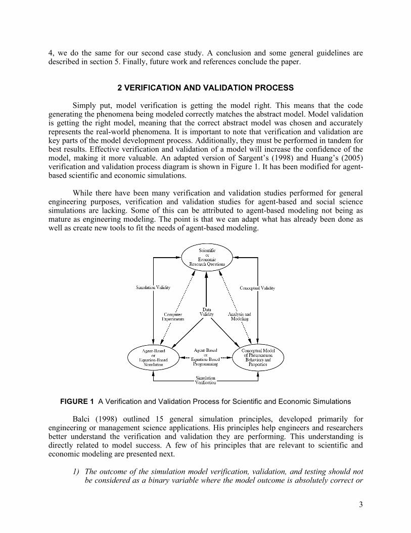
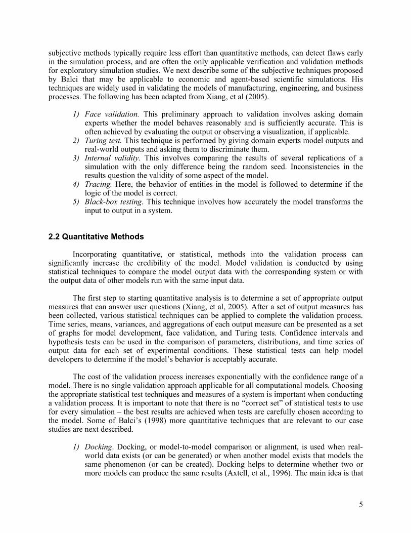
Simply put, model verification is getting the model right. This means that the code generating the phenomena being modeled correctly matches the abstract model. Model validation is getting the right model, meaning that the correct abstract model was chosen and accurately represents the real-world phenomena. It is important to note that verification and validation are key parts of the model development process. Additionally, they must be performed in tandem for best results. Effective verification and validation of a model will increase the confidence of the model, making it more valuable. An adapted version of Sargent’s (1998) and Huang’s (2005) verification and validation process diagram is shown in Figure 1. It has been modified for agent-based scientific and economic simulations.

While there have been many verification and validation studies performed for general

engineering purposes, verification and validation studies for agent-based and social science simulations are lacking. Some of this can be attributed to agent-based modeling not being as mature as engineering modeling. The point is that we can adapt what has already been done as well as create new tools to fit the needs of agent-based modeling.

FIGURE 1 A Verification and Validation Process for Scientific and Economic Simulations Balci (1998) outlined 15 general simulation principles, developed primarily for engineering or management science applications. His principles help engineers and researchers better understand the verification and validation they are performing. This understanding is directly related to model success. A few of his principles that are relevant to scientific and economic modeling are presented next.

1) The outcome of the simulation model verification, validation, and testing should not

be considered as a binary variable where the model outcome is absolutely correct or

4

incorrect. It is important to realize that models, being abstractions and not an absolute representation of a phenomenon, can never totally and exactly match a system.

2) Complete simulation model testing is not possible. As we cannot test all possible inputs and parameters for a system, we must choose the most appropriate ones.

3) Simulation model verification, validation, and testing must be planned and documented. Successful planning and documentation is critical and involves the work of many people throughout the lifetime of the system.

4) Successfully testing each submodel (module) does not imply overall model credibility. Simply because the modules work well independently does not mean they will work cohesively in a system.

When performing verification and validation on a model, it is good to begin by

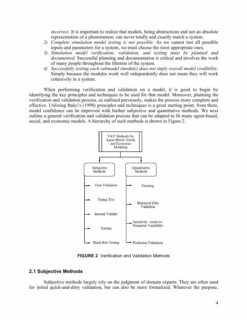
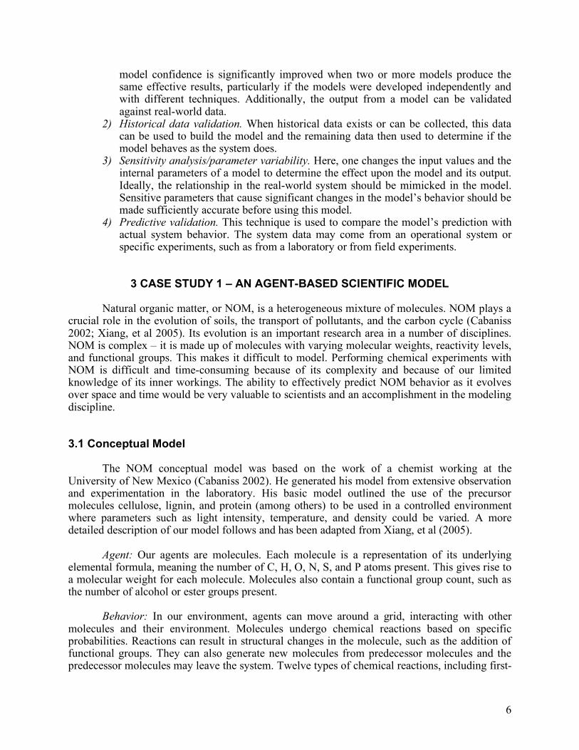
identifying the key principles and techniques to be used for that model. Moreover, planning the verification and validation process, as outlined previously, makes the process more complete and effective. Utilizing Balci’s (1998) principles and techniques is a great starting point; from there, model confidence can be improved with further subjective and quantitative methods. We next outline a general verification and validation process that can be adapted to fit many agent-based, social, and economic models. A hierarchy of such methods is shown in Figure 2.

FIGURE 2 Verification and Validation Methods 2.1 Subjective Methods Subjective methods largely rely on the judgment of domain experts. They are often used for initial quick-and-dirty validation, but can also be more formalized. Whatever the purpose,

5

subjective methods typically require less effort than quantitative methods, can detect flaws early in the simulation process, and are often the only applicable verification and validation methods for exploratory simulation studies. We next describe some of the subjective techniques proposed by Balci that may be applicable to economic and agent-based scientific simulations. His techniques are widely used in validating the models of manufacturing, engineering, and business processes. The following has been adapted from Xiang, et al (2005).

1) Face validation. This preliminary approach to validation involves asking domain experts whether the model behaves reasonably and is sufficiently accurate. This is often achieved by evaluating the output or observing a visualization, if applicable.

2) Turing test. This technique is performed by giving domain experts model outputs and real-world outputs and asking them to discriminate them.

3) Internal validity. This involves comparing the results of several replications of a simulation with the only difference being the random seed. Inconsistencies in the results question the validity of some aspect of the model.

4) Tracing. Here, the behavior of entities in the model is followed to determine if the logic of the model is correct.

5) Black-box testing. This technique involves how accurately the model transforms the input to output in a system.

2.2 Quantitative Methods Incorporating quantitative, or statistical, methods into the validation process can significantly increase the credibility of the model. Model validation is conducted by using statistical techniques to compare the model output data with the corresponding system or with the output data of other models run with the same input data.

The first step to starting quantitative analysis is to determine a set of appropriate output

measures that can answer user questions (Xiang, et al, 2005). After a set of output measures has been collected, various statistical techniques can be applied to complete the validation process. Time series, means, variances, and aggregations of each output measure can be presented as a set of graphs for model development, face validation, and Turing tests. Confidence intervals and hypothesis tests can be used in the comparison of parameters, distributions, and time series of output data for each set of experimental conditions. These statistical tests can help model developers to determine if the model’s behavior is acceptably accurate.

The cost of the validation process increases exponentially with the confidence range of a

model. There is no single validation approach applicable for all computational models. Choosing the appropriate statistical test techniques and measures of a system is important when conducting a validation process. It is important to note that there is no “correct set” of statistical tests to use for every simulation – the best results are achieved when tests are carefully chosen according to the model. Some of Balci’s (1998) more quantitative techniques that are relevant to our case studies are next described.

1) Docking. Docking, or model-to-model comparison or alignment, is used when real-world data exists (or can be generated) or when another model exists that models the same phenomenon (or can be created). Docking helps to determine whether two or more models can produce the same results (Axtell, et al., 1996). The main idea is that

6

model confidence is significantly improved when two or more models produce the same effective results, particularly if the models were developed independently and with different techniques. Additionally, the output from a model can be validated against real-world data.

2) Historical data validation. When historical data exists or can be collected, this data can be used to build the model and the remaining data then used to determine if the model behaves as the system does.

3) Sensitivity analysis/parameter variability. Here, one changes the input values and the internal parameters of a model to determine the effect upon the model and its output. Ideally, the relationship in the real-world system should be mimicked in the model. Sensitive parameters that cause significant changes in the model’s behavior should be made sufficiently accurate before using this model.

4) Predictive validation. This technique is used to compare the model’s prediction with actual system behavior. The system data may come from an operational system or specific experiments, such as from a laboratory or from field experiments.

3 CASE STUDY 1 – AN AGENT-BASED SCIENTIFIC MODEL

Natural organic matter, or NOM, is a heterogeneous mixture of molecules. NOM plays a crucial role in the evolution of soils, the transport of pollutants, and the carbon cycle (Cabaniss 2002; Xiang, et al 2005). Its evolution is an important research area in a number of disciplines. NOM is complex – it is made up of molecules with varying molecular weights, reactivity levels, and functional groups. This makes it difficult to model. Performing chemical experiments with NOM is difficult and time-consuming because of its complexity and because of our limited knowledge of its inner workings. The ability to effectively predict NOM behavior as it evolves over space and time would be very valuable to scientists and an accomplishment in the modeling discipline. 3.1 Conceptual Model

The NOM conceptual model was based on the work of a chemist working at the University of New Mexico (Cabaniss 2002). He generated his model from extensive observation and experimentation in the laboratory. His basic model outlined the use of the precursor molecules cellulose, lignin, and protein (among others) to be used in a controlled environment where parameters such as light intensity, temperature, and density could be varied. A more detailed description of our model follows and has been adapted from Xiang, et al (2005).

Agent: Our agents are molecules. Each molecule is a representation of its underlying

elemental formula, meaning the number of C, H, O, N, S, and P atoms present. This gives rise to a molecular weight for each molecule. Molecules also contain a functional group count, such as the number of alcohol or ester groups present.

Behavior: In our environment, agents can move around a grid, interacting with other

molecules and their environment. Molecules undergo chemical reactions based on specific probabilities. Reactions can result in structural changes in the molecule, such as the addition of functional groups. They can also generate new molecules from predecessor molecules and the predecessor molecules may leave the system. Twelve types of chemical reactions, including first-

7

and second-order chemical reactions are modeled as described in Table 1. The categories of reactions are as follows:

1) First order reactions with a split. The predecessor molecule A is split into two

successor molecules B and C. Molecule B occupies the position of molecule A, while one of the empty cells closest to molecule B is filled with molecule C.

2) First order reactions without a split. The transformation only changes the structure of the predecessor molecule A.

3) First order reactions with the disappearance of a molecule. The predecessor molecule A disappears from the system.

4) Second order reactions. Two molecules A and B are combined to form a new molecule C. Molecule C replaces molecule A and molecule B is removed from the system.

TABLE 1 Chemical Reactions

Name Type Ester Condensation Second order Ester Hydrolysis First order with a split Amide Hydrolysis First order with a split Microbial Uptake First order with the

disappearance of a molecule Dehydration First order with a split Strong C=C Oxidation First order with a split (50% of

the time) Mild C=C Oxidation First order without a split Alcohol C-O-H Oxidation First order without a split Aldehyde C=O Oxidation First order without a split Decarboxylation First order without a split Hydration First order without a split Aldol Condensation Second order

Space: In the NOM model, the agents are associated with a location in 2D geometrical

space and can move around their environment. Each cell on the grid can host multiple molecules up to a certain threshold.

Reaction Probabilities: The probability for each reaction type is expressed in terms of

intrinsic and extrinsic factors. Intrinsic factors are derived from the molecular structure including the number of functional groups and many other structural factors. Extrinsic factors arise from the environment and include concentrations of inorganic chemical species, light intensity, availability of surfaces, presence of microorganisms, presence and concentration of extracellular enzymes, and the presence and reactivity of other NOM molecules. The intrinsic and extrinsic factors are combined in probabilistic functions.

Molecular Properties: The reactivity of the resulting NOM over time can be predicted

based on the distributions of molecular properties, which are calculated from the elemental composition and functional group data. They represent a measurable quantity that can be used as a predictor for environmental function and are useful for the calibration and verification of our conceptual model and simulation.

8

Simulation Process: The conceptual model is a stochastic synthesis model of NOM

evolution, meaning the state of the system is represented by a set of values with a certain probability distribution, such that the evolution of the system is dependent on a series of probabilistic discrete events. At each time step, for each molecule, a uniform random number is generated. This number determines whether a reaction will occur, and if one does occur, its reaction type. After a reaction takes place, the attributes for the current molecule are updated and the reaction probabilities are recalculated. The molecule structure is changed to alter the outcome of the reaction and a new probability table entry is added for newly formed molecules, if there are any.

3.2 Implementations

The NOM conceptual model was initially implemented in Pascal, resulting in a program for Windows called AlphaStep. Our implementation is coded using Java (Sun JDK 1.4.2) and the Repast toolkit. Repast is an agent-based simulation toolkit written in Java. It contains a control panel to control and manipulate the model and has rich visualization capabilities. We chose Java for our model because we also incorporate a web-based front end to the system where users can create and submit simulations, as well as view graphical results.

3.3 Validation We followed the general technique previously outlined when validating the NOM model. We began with subjective analysis and then proceeded with quantitative analysis. 3.3.1 Subjective Analysis

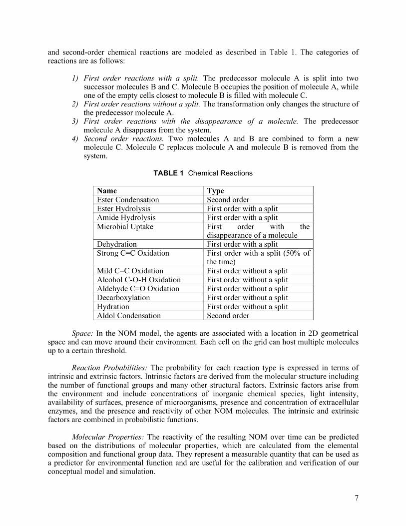
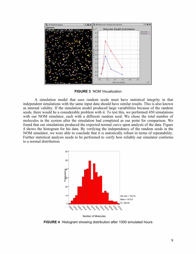
The validation of the NOM model began with face validation of the conceptual model by domain experts. They evaluated the underlying mechanisms and properties and drew their conclusions. After achieving initial face validation, coding of the agent-based simulation took place. In this step, verification methods such as code walk-through, trace analysis, input-output testing, pattern testing, boundary testing, code debugging, and calculation verification were used to verify the correctness of the simulation. Another useful technique used for simulation validation is visualization (Grimm 2002). Visualization is often used in conjunction with face validation. A snapshot of an animated visualization of the flow of molecules through a soil column is shown in Figure 3. A corresponding animated graph of the molecular weight distribution shows how the molecular weight distribution shifts with time: initially favoring lower weight molecules and gradually shifting to larger molecular weights as the simulated time passes. These same behaviors were observed in the laboratory, which increases confidence in the simulation.

9

FIGURE 3 NOM Visualization

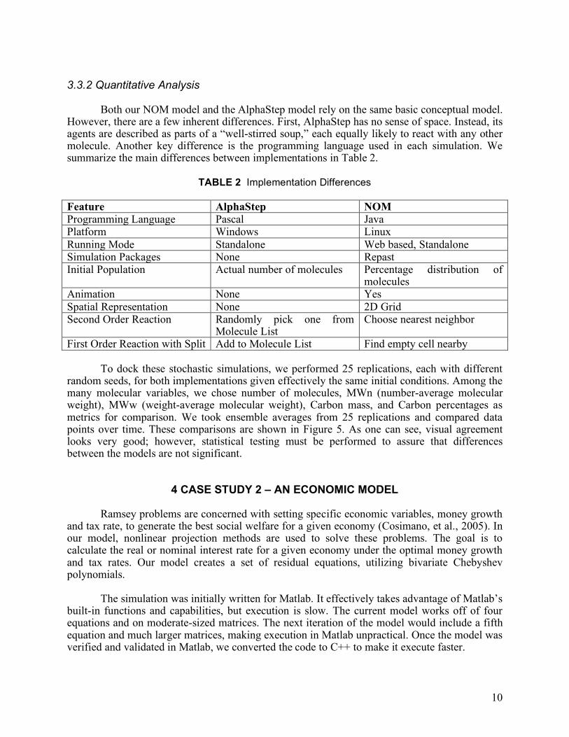
A simulation model that uses random seeds must have statistical integrity in that independent simulations with the same input data should have similar results. This is also known as internal validity. If the simulation model produced large variabilities because of the random seeds, there would be a considerable problem with it. To test this, we performed 450 simulations with our NOM simulator, each with a different random seed. We chose the total number of molecules in the system after the simulation had completed as our point for comparison. We found that our simulations produced the expected normal curve upon analysis of the data. Figure 4 shows the histogram for his data. By verifying the independency of the random seeds in the NOM simulator, we were able to conclude that it is statistically robust in terms of repeatability. Further statistical analysis needs to be performed to verify how reliably our simulator conforms to a normal distribution.

Number of Molecules

1775.0

1725.0

1675.0

1625.0

1575.0

1525.0

1475.0

1425.0

1375.0

1325.0

1275.0

1225.0

Fre

qu

en

cy

60

50

40

30

20

10

0

Std. Dev = 100.79

Mean = 1473.9

N = 450.00

FIGURE 4 Histogram showing distribution after 1000 simulated hours

10

3.3.2 Quantitative Analysis

Both our NOM model and the AlphaStep model rely on the same basic conceptual model.

However, there are a few inherent differences. First, AlphaStep has no sense of space. Instead, its agents are described as parts of a “well-stirred soup,” each equally likely to react with any other molecule. Another key difference is the programming language used in each simulation. We summarize the main differences between implementations in Table 2.

TABLE 2 Implementation Differences

Feature AlphaStep NOM Programming Language Pascal Java Platform Windows Linux Running Mode Standalone Web based, Standalone Simulation Packages None Repast Initial Population Actual number of molecules Percentage distribution of

molecules Animation None Yes Spatial Representation None 2D Grid Second Order Reaction Randomly pick one from

Molecule List Choose nearest neighbor

First Order Reaction with Split Add to Molecule List Find empty cell nearby

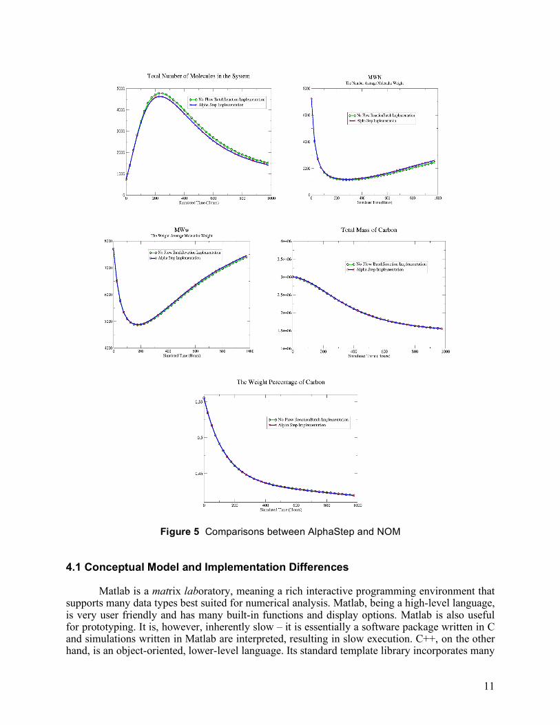
To dock these stochastic simulations, we performed 25 replications, each with different random seeds, for both implementations given effectively the same initial conditions. Among the many molecular variables, we chose number of molecules, MWn (number-average molecular weight), MWw (weight-average molecular weight), Carbon mass, and Carbon percentages as metrics for comparison. We took ensemble averages from 25 replications and compared data points over time. These comparisons are shown in Figure 5. As one can see, visual agreement looks very good; however, statistical testing must be performed to assure that differences between the models are not significant.

4 CASE STUDY 2 – AN ECONOMIC MODEL

Ramsey problems are concerned with setting specific economic variables, money growth and tax rate, to generate the best social welfare for a given economy (Cosimano, et al., 2005). In our model, nonlinear projection methods are used to solve these problems. The goal is to calculate the real or nominal interest rate for a given economy under the optimal money growth and tax rates. Our model creates a set of residual equations, utilizing bivariate Chebyshev polynomials.

The simulation was initially written for Matlab. It effectively takes advantage of Matlab’s built-in functions and capabilities, but execution is slow. The current model works off of four equations and on moderate-sized matrices. The next iteration of the model would include a fifth equation and much larger matrices, making execution in Matlab unpractical. Once the model was verified and validated in Matlab, we converted the code to C++ to make it execute faster.

11

Figure 5 Comparisons between AlphaStep and NOM

4.1 Conceptual Model and Implementation Differences

Matlab is a matrix laboratory, meaning a rich interactive programming environment that supports many data types best suited for numerical analysis. Matlab, being a high-level language, is very user friendly and has many built-in functions and display options. Matlab is also useful for prototyping. It is, however, inherently slow – it is essentially a software package written in C and simulations written in Matlab are interpreted, resulting in slow execution. C++, on the other hand, is an object-oriented, lower-level language. Its standard template library incorporates many

12

desirable functions and it is relatively simple to code. Because it has an efficient compiler and is a lower-level language, simulations written directly in C++ run much faster than equivalent simulations written in Matlab.

Converting the simulation from Matlab to C++ was much more difficult than expected. In Matlab, variables are not declared as they are in C++. Instead, most variables are assumed to be arrays. These arrays can contain real numbers, complex numbers, or even other arrays of real numbers, among other things. This creates a big problem in C++, as variables must be declared with a data type. For example, the variable array1 could represent an array of real numbers at one point in a Matlab program and an array of complex numbers at another point. The idea is that the variable array1 is in essence overloaded to handle many data types. In C++, functions operate and are called differently depending on the type of data passed to them. Overcoming this step was pivotal to porting the code.

Another main difficulty in going from Matlab to C++ was emulating Matlab’s built-in functions. The majority of the Matlab functions utilized in this simulation are part of the LAPACK, or linear algebra package, and include functions such as taking the normal of a matrix or vector, inverting a matrix, conditioning a matrix, and the like. Not only are these not inherently included in C++, but they are again overloaded in the sense that you can pass Matlab’s max function a vector, a matrix, or a simple set of numbers and it will give the proper result. While it is possible to call Matlab from within C++ to make use of such functions, the desire of this project was to have everything run in C++ for maximum speed. Determining the inner workings of Matlab’s many functions and implementing approximations of them in C++ proved difficult and time-consuming. In the end, the core of the simulations did the same thing, but with an inherently different implementation, requiring a rigorous verification and validation effort. 4.2 Performance

Results from runs of 5, 50, and 500 iterations of the simulation can be found in Table 3. As evidenced in the table, the speedup is significant, or approximately 30 times faster in C++.

TABLE 3 Performance over multiple iterations

5 Iterations 50 Iterations 500 Iterations Matlab 58 seconds 568 seconds 8872 seconds C++ 2 seconds 17 seconds 176 seconds

4.3 Validation Validating the economic model was a little different than with the scientific model described in the first case study. The validation process helped us identify some problems with the C++ implementation, so we were limited in the amount of quantitative analysis that we could perform. In this case, validation served the purpose of identifying what was wrong with our implementation.

13

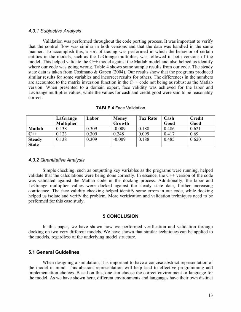
4.3.1 Subjective Analysis Validation was performed throughout the code porting process. It was important to verify

that the control flow was similar in both versions and that the data was handled in the same manner. To accomplish this, a sort of tracing was performed in which the behavior of certain entities in the models, such as the LaGrange multiplier, was followed in both versions of the model. This helped validate the C++ model against the Matlab model and also helped us identify where our code was going wrong. Table 4 shows some sample results from our code. The steady state data is taken from Cosimano & Gapen (2004). Our results show that the programs produced similar results for some variables and incorrect results for others. The differences in the numbers are accounted to the matrix inversion function in the C++ code not being as robust as the Matlab version. When presented to a domain expert, face validity was achieved for the labor and LaGrange multiplier values, while the values for cash and credit good were said to be reasonably correct.

TABLE 4 Face Validation

LaGrange

Multiplier Labor Money

Growth Tax Rate Cash

Good Credit Good

Matlab 0.138 0.309 -0.009 0.188 0.486 0.621 C++ 0.123 0.309 0.248 0.099 0.417 0.69 Steady State

0.138 0.309 -0.009 0.188 0.485 0.620

4.3.2 Quantitative Analysis

Simple checking, such as outputting key variables as the programs were running, helped validate that the calculations were being done correctly. In essence, the C++ version of the code was validated against the Matlab code in the docking process. Additionally, the labor and LaGrange multiplier values were docked against the steady state data, further increasing confidence. The face validity checking helped identify some errors in our code, while docking helped us isolate and verify the problem. More verification and validation techniques need to be performed for this case study.

5 CONCLUSION In this paper, we have shown how we performed verification and validation through docking on two very different models. We have shown that similar techniques can be applied to the models, regardless of the underlying model structure. 5.1 General Guidelines When designing a simulation, it is important to have a concise abstract representation of the model in mind. This abstract representation will help lead to effective programming and implementation choices. Based on this, one can choose the correct environment or language for the model. As we have shown here, different environments and languages have their own distinct

14

advantages and disadvantages. It is upon these that our programming decisions must be based. It is important to note that the entire lifetime of the model must be considered when making these decisions. The choices must also be made with consideration to the verification and validation techniques that will be applied to the model. These verification and validation techniques must also be thought out in advance.

6 FUTURE WORK

In future studies, it is important that we use and develop more stringent and formalized verification and validation testing methods. Doing this on top of a strong statistical foundation would further increase confidence of the models. Gathering empirical data and generating statistical data would also serve as a better point of comparison when comparing our models with real-world systems. Additionally, performing some goodness-of-fit tests, such as the Chi-Square test and the Kolmogorov-Smirnoff test, as well as performing the ANOVA test would help us to determine the validity of the models. Finally, improving on the helper functions in the C++ version of the second case study would both speed up and strengthen the results for that model. It would also allow us to do a more in-depth verification and validation study for the second case study. References AlphaStep. http://www.nd.edu/~nom/Software/software.html Axtell, R., Axelrod, R., Epstein, J.M., Cohen, M.D., “Aligning Simulation Models: A Case

Study and Results,” Computational and Mathematical Organization Theory, 1996. Balci, O., “Handbook of Simulation: Principles, Methodology, Advances, Applications, and

Practice,” Book Chapter: Verification, Validation, and Testing, John Wiley & Sons, New York, 1998.

Banks, J., Carson III, J.S., Nelson, B.L., Nicol, D.M., “Discrete-Event System Simulation,”

Prentice Hall International Series in Industrial and Systems Engineering, Fourth Edition, 2005.

Cabaniss, S.E., “Modeling and Stochastic Simulation of NOM Reactions,” Working Paper;

available at http://www.nd.edu/~nom/Papers/WorkingPapers.pdf. Cosimano, T.F., Gapen, M.T., “Optimal Fiscal and Monetary Policy with Nominal and Indexed

Debt,” Working Paper, available at http://www.nd.edu/%7Etcosiman/Optimapolicy.pdf. Cosimano, T.F., Gapen, M.T., “Solving Ramsey Problems with Nonlinear Projection Methods,”

Studies in Nonlinear Dynamics & Econometrics, Vol. 9, Spring 2005. Grimm, V., “Visual Debugging: A Way of Analyzing, Understanding, and Communicating

Bottom-Up Simulation Models in Ecology,” Natural Resource Modeling, Vol. 15, No. 1, pp 23-38, Spring 2002.

15

Huang, Y., Xiang, X., Madey, G., Cabaniss, S., “Agent-Based Scientific Simulation,” IEEE

Computing in Science & Engineering, Vol. 7, No. 1, pp. 22-29, January/February 2005. Matlab. http://www.mathworks.com/products/matlab/. Repast. http://repast.sourceforge.net/. Sargent, R.G., “Validation and Verification of Simulation Models,” in Proceedings of the 1998

Winter Simulation Conference, pp. 121-130, 1998. Xiang, X., Kennedy, R., Madey, G., “Verification and Validation of Agent-based Scientific

Simulation Models,” Agent-Directed Simulation Conference, San Diego, CA, April 2005.