Embed Size (px)
Citation preview
AVACS – Automatic Verification and Analysis ofComplex Systems
REPORTSof SFB/TR 14 AVACS
Editors: Board of SFB/TR 14 AVACS
Verification Architectures:Compositional Reasoning for Real-time Systems
byJohannes Faber
AVACS Technical Report No. 65August 2010
ISSN: 1860-9821
Publisher: Sonderforschungsbereich/Transregio 14 AVACS(Automatic Verification and Analysis of Complex Systems)
Editors: Bernd Becker, Werner Damm, Martin Fränzle, Ernst-Rüdiger Olderog,Andreas Podelski, Reinhard Wilhelm
ATRs (AVACS Technical Reports) are freely downloadable from www.avacs.org
Copyright c© August 2010 by the author(s)Author(s) contact: Johannes Faber ([email protected]).
Verification Architectures:Compositional Reasoning for Real-time Systems?
Johannes Faber
Department of Computing Science, University of Oldenburg, [email protected]
Abstract. We introduce a conceptual approach to decompose real-timesystems, specified by integrated formalisms: instead of showing safetyof a system directly, one proves that it is an instance of a VerificationArchitecture, a safe behavioural protocol with unknowns and local real-time assumptions. We examine how different verification techniques canbe combined in a uniform framework to reason about protocols, assump-tions, and instantiations of protocols. The protocols are specified in CSP,extended by data and unknown processes with local assumptions in areal-time logic. To prove desired properties, the CSP dialect is embed-ded into dynamic logic and a sequent calculus is presented. Further, weanalyse the instantiation of protocols by combined specifications, here il-lustrated by CSP-OZ-DC. Using an example, we show that this approachhelps us verify specifications that are too complex for direct verification.
1 Introduction
In the analysis of real-time systems, several aspects have to be covered, e.g.,(1) behaviour that conforms to communication protocols, (2) rich data struc-tures, and (3) timing constraints such that the system reacts timely to externalevents. Thus, in practise it turns out that, to adequately handle those systems,engineers fall back on combinations of techniques. An example is the wide ac-ceptance of the UML, combining multiple graphical notations for different viewsof a design. Similarly, in the world of formal analysis there has been a lot ofwork on integrating specification techniques to condense advantages of singleformalisms into combined formalisms, e.g., [2,25,19,1,10,32,28,15,29]. However,a major problem remains: these integrated techniques are designed for hetero-geneous systems, i.e., they cover several different aspects, and when formallyverifying those systems we have to cope with their inherent complexity.
We thus propose a Verification Architecture approach to verify global prop-erties by combining local analyses. This idea originates from previous case stud-ies [21], where we decomposed a train control system according to its abstractbehavioural protocol that splits the system runs into several phases (e.g., brak-ing, running) with local real-time properties that hold during these phases. Aftershowing the correctness of a desired global property for this protocol, the global? This paper is an extended version of [9].
2
property is also guaranteed by all instances of the protocol for that the localproperties are satisfied. We generalise and formalise this approach in the con-text of combined languages. The approach is structured into several layers:
1. abstract behavioural protocols with unknowns, that have a large degree offreedom to comprise a large class of concrete systems, need to be specifiedand verified with respect to desired safety properties;
2. since the analysed systems are often time-dependent it is important to allowimposing of additional real-time assumptions on protocol phases and it mustbe possible to verify the protocols taking these assumptions into account;
3. it needs to be checked that concrete models, given as combined specificationsto capture heterogeneous systems, are instantiations of the protocol;
4. it needs to be checked that concrete models actually guarantee the assump-tions on the protocol phases.
The challenge is to tackle each layer of the problem with a suitable formalisationand to integrate the heterogeneous formalisations into a uniform framework.
As several combined specification formalisms base on Communicating Se-quential Processes (CSP) [14,26], we propose to use CSP to specify system pro-tocols with unknowns. Thus, we define a CSP extension by data constraints andunknown processes and show that it is suited to specify abstract system proto-cols. In addition, we allow the unknown processes to be constrained by formulaein an arbitrary temporal logic. We call this combination of protocol with localassumptions Verification Architecture (VA). To establish safety properties onVAs, we embed our CSP extension into a temporal dynamic logic [12,22] andintroduce a sound sequent-style calculus [11] over this logic that allows for es-tablishing desired properties under local real-time assumptions. We prove thatall specifications that refine the architecture’s CSP part and for that the localassumptions are valid directly inherit the desired properties.
To exemplify the instantiation of VAs by a combined specification language,we choose CSP-OZ-DC (COD) as instantiation language and Duration Calcu-lus (DC) [34,33] for the local assumptions on protocol phases. We introduce asimple syntactical proof rule to show efficiently that a concrete specification isa VA refinement. The correctness of the local assumptions can be shown usingan established model checking approach for COD and DC [21]. Using a runningexample motivated by the European Train Control System (ETCS) [7], we pro-vide evidence that our method enables the verification of a system that is toolarge to be verified without decomposition techniques.
We summarise our contributions:
Section 1 We provide a new conceptional approach on how to use behaviouralprotocols, called Verification Architectures (VA), as a decomposition techniqueto enable verification of realistic systems specified by combined formalisms.Section 2 We introduce a CSP dialect with data, unknown process parts, andlocal real-time assumptions for the specification of VAs.Section 3 A new sequent-style calculus over this CSP dialect allows us to verifydesired properties of VAs. We establish basic properties of the calculus.
3
Section 4 We examine the instantiation of VAs by COD specifications and givea proof rule to syntactically check refinement relations.
1.1 Discussion of Related Work
Our approach is inspired by [3], where for a fixed DC protocol a design patternfor cooperating traffic agents is introduced. Also, [3] motivates the work of [17],in which CSP-OZ-DC patterns are applied as a formal counterpart to somestandard patterns from software engineering. In contrast to our approach noformal framework for the use, application, and verification of design patternsis introduced. A general view on formalisation techniques for design patternsis given in [30], but there, verification of real-time systems is not considered.[6] presents an approach using patterns for a combined real-time language: timedautomata patterns for a set of timing constraints are formally linked to TCOZ.
The work [18] introduces context systems that can be instantiated with con-crete processes, a concept similar to the unknown processes of this paper. Theyconsider arbitrary process algebras as context systems and the generation ofcompositional assumptions in Hennessy-Milner logic whereas we use a fixed pro-cess algebra but allow arbitrary real-time logics for the assumptions. In [18], noreal-time aspects and no data aspects are considered.
Our approach can be seen as Assume-Guarantee reasoning in the context ofcombined, parametric specifications, because we show validity of global prop-erties assuming local component properties. [4] contains a general introductioninto Assume-Guarantee reasoning without time and without the context of con-joint verification techniques. In [20] a verification approach for CSP-OZ (withouttime) is investigated that does not consider decompositions by given protocolsbut instead uses a learning-based algorithm to generate assumptions on lay-ered components. [5] presents an Assume-Guarantee based, sound and completeproof system to reason about CCS processes with Hennessy-Milner assumptionson the environment of processes. In contrast to the approach of this paper, theseunknown parts with assumptions are not explicitly represented as process ex-pressions and, thus, are always composed in parallel to the known process of thesystem. In addition, neither real-time properties, data constraints, nor combinedspecifications are considered. Both approaches have in common that concretesystems instantiating the unknown parts and satisfying the assumptions inheritthe properties of the abstract system.
Our CSP extension by data and unknown processes enables us to specifyparametric systems because (1) we can use global data parameters and (2) un-known processes give a parametric view to process components that are not fixedbut represent a class of concrete processes. In doing so, we provide a general for-malism that is on the one hand flexible enough to express behavioural protocolswith a large degree of freedom and on the other hand integrates well with com-bined specification formalisms based on CSP [19,10,32,28,15,29]. So, our goalwas not to introduce a further combination of CSP with data as a replacementfor existing formalisms but to provide a notation for VAs that can be used in
4
combination with these formalisms. It turned out that direct usage of a com-bined formalism like [15] is not appropriate for a proof rule approach because ofthe complex combination of languages in an object-oriented structure.
[22,23] introduce a sequent calculus for temporal dynamic logic to verify tem-poral properties for hybrid systems; they also examine fragments of the ETCSas case study. The work [16] introduces a sequent calculus to verify the Javapart of JCSP programs and a translation to Petri nets for the CSP library calls.Recursion in CSP processes and timing constraints are not considered.
Our instantiation rule for COD is not intended to be complete—it is definedas an efficient syntactic refinement check. General results on refinement or sub-typing in CSP-OZ and related formalisms can be found in [10] and [31].
1.2 The Verification Architecture Approach
Let prtcl(p,P1, . . .Pn) be an abstract behavioural protocol depending on a vec-tor of data parameters p and process parameters Pi . Additionally, we considerassumptions in a temporal logic on the Pi , asm1(p), . . . , asmn(p), that also de-pend on the parameters. We denote the combination of behavioural protocol andtemporal assumptions as Verification Architecture (VA). Our aim is to show thata safety property safe(p) is valid for every possible model that is a refinementof the behavioural protocol and that respects the assumptions.
To apply our approach, we have to show that the VA is correct, i.e., theprotocol is correct for all parameters and processes respecting the assumptions:
∀ p,Pi • (∧
i=1,...,n
Pi |= asmi(p))⇒ (prtcl(p,P1, . . . ,Pn) |= safe(p)) (1)
This verification task to verify the correctness of the parametric VA is for realisticsystems not necessarily easy and we will provide proof rules for the verification.But once it is verified, this result is reusable as all instantiations of this archi-tecture inherit the correctness property automatically. We only have to showthat a potential instantiation is a refinement of the protocol and that the localassumptions are valid, which is due to their locality easier than to verify theglobal property directly. To be more concrete, we consider the concrete modelspec(p,P0
1 , . . . ,P0n), where the P0
i are instantiations of the process parameters.Firstly, we have to show that every trace of this model (without assumptions)is also a trace of the protocol:
∀ p • [[spec(p,P01 , . . . ,P
0n)]] ⊆ [[prtcl(p,P0
1 , . . . ,P0n)]]. (2)
This refinement relation on the processes can be shown syntactically for a specificclass of instantiations (cf. Sect. 4). Thus, it is easy to verify. Secondly, we haveto show that the assumptions are valid for the concrete specification:
∀ p • P0i |= asmi(p) for all i = 1..n. (3)
This can be done by applying existing verification techniques for the language ofthe assumptions. With this, our approach yields that the desired safety property
5
is valid for the concrete model. We argue that this proposition is correct. From(1) and (3) we can conclude (4) and with (2) we get the desired property (5).
∀ p • prtcl(p,P01 , . . . ,P
0n) |= safe(p) (4)
∀ p • spec(p,P01 , . . . ,P
0n) |= safe(p) (5)
We summarise that if a correct VA is given, we only have to show that, firstly,the model’s process is a refinement of the abstract protocol and, secondly, themodel respects the assumptions. Then, we say that the model is an instantiationof the VA and we can conclude that it inherits the VA’s correctness.
2 CSP Processes with Data Constraints and Unknowns
In this section, we introduce a CSP extension by data constraints and unknownprocesses to specify Verification Architectures (VA).
For specifying VAs, a high degree of freedom is necessary to handle generalpatterns of parametric systems with data. To this end, we extend CSP by dataconstraints to define state changes and by a new construct, so-called unknownprocesses. Unknown processes are special processes that allow the occurrence ofarbitrary events except for events from a fixed alphabet and arbitrary changesof variables except for variables from a fixed set. They can terminate and maybe restricted by constraints from an arbitrary real-time logic.
Syntax. We consider many-sorted first order formulae FormΣ from a signa-ture Σ = (Sort ,Symb,Var ,Par) with primed and unprimed system variablesand functions Symb with sorts Sort , variables Var , and parameters Par withfixed but arbitrary values. The syntax of CSP processes with data and unknownprocesses is given by
P ::= Stop | Skip | (a • ϕ)→ P | P1 2 P2 | P1‖|P2 | P1 ‖A P2 | P1o9 P2 | X
| (Proc\A,V •F ) | (Proc∞\A,V •F ),
where a ∈ Events,A ⊆ Events, ϕ ∈ FormΣ , V ⊆ Symb and F is a constraintin a temporal logic with the same semantical domain as CSP with data con-straints. In this definition, a difference to the standard CSP definition is thatwe have constrained occurrences of events a by formulae ϕ, denoted a • ϕ. Theintuition is that when the event a occurs the state space is changed accordingto the constraint ϕ, where unprimed symbols in ϕ refer to valuations before theoccurrence of a and primed symbols to the valuations after a. The intuition be-hind an unknown process like (Proc\a,b,v • F ) is that during the executionof the process arbitrary behaviour is allowed provided that the formula F is notviolated. The events a and b are forbidden and the system variable v cannot bechanged in this execution. A process Proc∞ marked with∞ will never terminate.
6
RBC
︸ ︷︷ ︸RD︸ ︷︷ ︸
sf︸ ︷︷ ︸MA
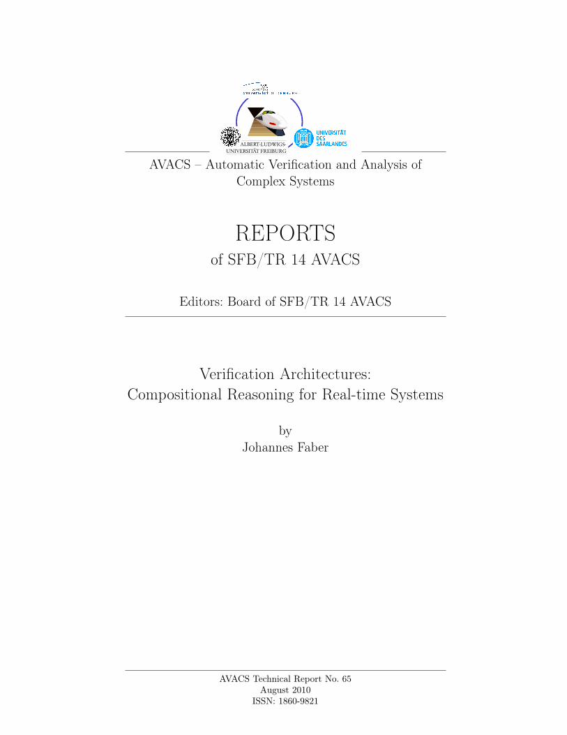
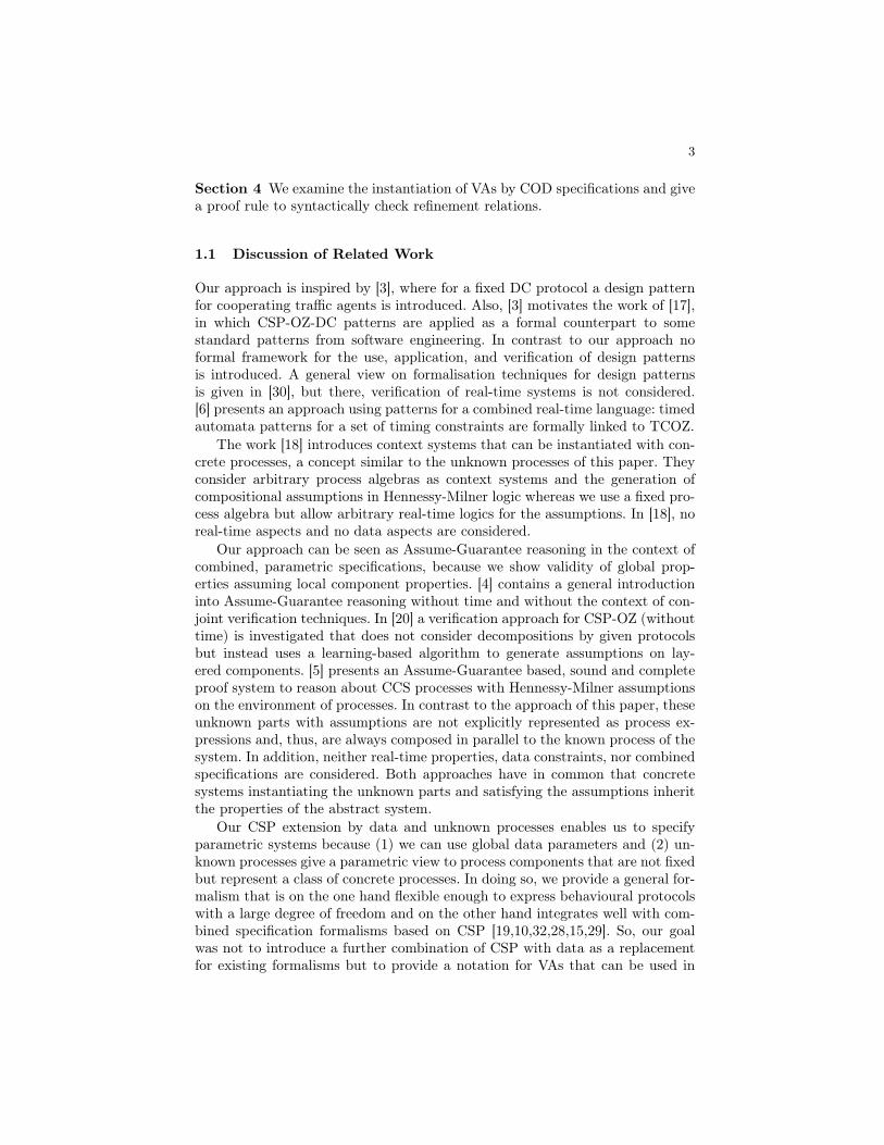
Fig. 1. Example: ETCS
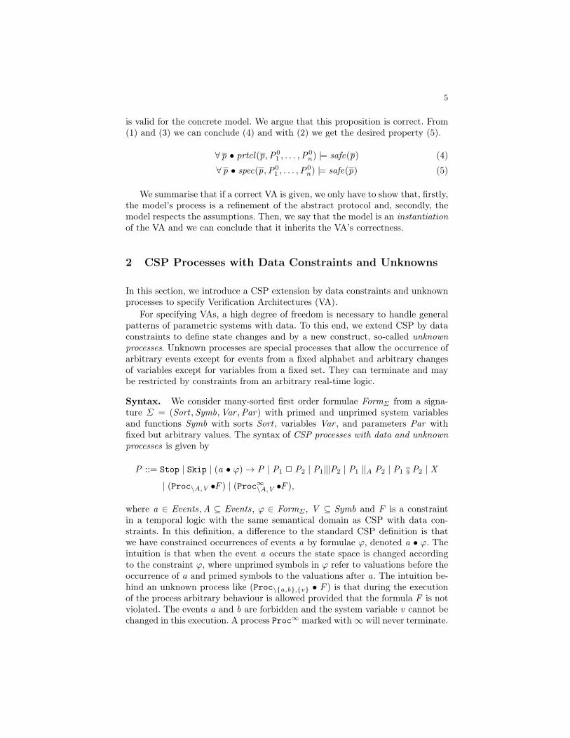
Example 1. As a running example we consider a sys-tem motivated by the European Train Control Sys-tem (ETCS) [7]. The setting is pictured in Fig. 1: aso-called Radio Block Center (RBC) grants move-ment authorities (MA) to a train. The system isconsidered safe as long as the train stays within theMA. The distance of the train to the end of the MAis given by a real-valued variable sf , reflecting thesafety of the system that shall never be below orequal to 0. The position RD is the last position atwhich the train needs to apply the brakes to stopin time. The train can request extensions of MAs atany time.
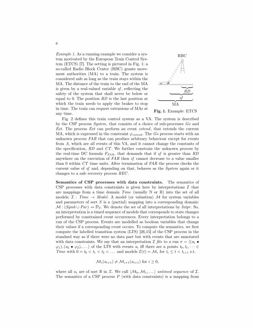
Fig. 2 defines this train control system as a VA. The system is describedby the CSP process System, that consists of a choice of sub-processes Go andExt . The process Ext can perform an event extend , that extends the currentMA, which is expressed in the constraint ϕextend . The Go process starts with anunknown process FAR that can produce arbitrary behaviour except for eventsfrom A, which are all events of this VA, and it cannot change the constants ofthe specification, RD and CT . We further constrain the unknown process bythe real-time DC formula FFAR, that demands that if sf is greater than RDanywhere on the execution of FAR then sf cannot decrease to a value smallerthan 0 within CT time units. After termination of FAR the process checks thecurrent value of sf and, depending on that, behaves as the System again or itchanges to a safe recovery process REC .
Semantics of CSP processes with data constraints. The semantics ofCSP processes with data constraints is given here by interpretations I thatare mappings from a time domain Time (usually N or R) into the set of allmodels: I : Time → Model . A model (or valuation) M for system variablesand parameters of sort S is a (partial) mapping into a corresponding domain:M : (Symb ∪ Par) 7→ DS . We denote the set of all interpretations by Intpr . So,an interpretation is a timed sequence of models that corresponds to state changesperformed by constrained event occurrences. Every interpretation belongs to arun of the CSP process. Events are modelled as boolean variables that changetheir values if a corresponding event occurs. To compute the semantics, we firstcompute the labelled transition system (LTS) [26,15] of the CSP process in thestandard way as if there were no data part but with events that are annotatedwith data constraints. We say that an interpretation I fits to a run π = 〈(a1 •ϕ1), (a2 • ϕ2), . . . 〉 of the LTS with events ai iff there are a points t0, t1, · · · ∈Time with 0 = t0 < t1 < t2 < . . . and models I(t) =Mi for ti ≤ t < ti+1 s.t.
Mi(ai+1) 6=Mi+1(ai+1) for i ≥ 0,
where all ai are of sort B in Σ. We call 〈M0,M1, . . . 〉 untimed sequence of I.The semantics of a CSP process P (with data constraints) is a mapping from
7
System c= Go 2 Ext
Ext c= (extend • ϕextend)→ System
Go c= FAR o
9 (check • ϕcheck )→ ((fail • ϕfail)→ REC 2 (pass • ϕpass)→ System)
ϕextend = sf ′ > sfϕcheck = Ξ(sf ) ∧ sf ≤ RD ∧ ¬ok ′
∨ Ξ(sf ) ∧ sf > RD ∧ ok ′
ϕfail = Ξ(sf ) ∧ ¬okϕpass = Ξ(sf ) ∧ ok
FAR c= Proc\A,C • FFAR
REC c= Proc
∞\A,C • FREC
FFAR = ¬3(` > CT ) ∧
¬3(dsf > RDea` < CT adsf ≤ 0e)
FREC = ¬3(dsf > 0eadsf ≤ 0e)A = check , fail , pass, extend,C = RD ,CT
Fig. 2. VA for a train control system
models to sets of interpretations: [[·]] : Model → PIntpr . An interpretation isvalid, I ∈ [[P ]]M, iff it respects the state changes of the process, i.e., iff
1. there is a run π = 〈(a1 • ϕ1), (a2 • ϕ2), . . . 〉 of the LTS of P such that I fitsto π. Let the resulting untimed sequence be 〈M0,M1, . . . 〉.
2. M0 =M3. (Mi−1 ∪M′i) |= ϕi for i > 04. Mi(v) =Mi+1(v) for all parameter v ∈ Par and i ≥ 05. if ai = X thenMi−1(v) =Mi(v) for all symbols v ∈ Symb.
The modelM′i is a model for primed symbols, i.e.,M′i(f ′) =Mi(f ), and X thetermination symbol of CSP. Note that this definition makes use of CSP’s tracesemantics. One consequence is that we do not have to distinguish external andinternal choice that are equivalent in the trace semantics.
Semantics of unknown processes. The definition above does not captureunknown processes with data constraints. Even though a process Proc\A,V with-out temporal constraints can be rewritten to a standard CSP process, we needto take care of the additional constraints. Since these constraints need to bevalid everywhere on all traces of the process we do not give (single step) transi-tion rules for constrained unknown processes. Instead, we give transition rules tocompute the LTS of unconstrained processes and we additionally demand thatfor every trace of those processes the constraint is also valid. The set of transitionrules for computing the LTS of a CSP process is extended by the rules
Proc(∞)\A,V
a•ΞV−→ Proc(∞)\A,V Proc\A,V
X−→ Ω,
in which a ∈ UEvents \ A, i.e., a is in the universe of events (without τ) exceptA. The process can perform an arbitrary event that is not in the set A and theevent’s constraint ensures that symbols from the set V are not changed, whichis expressed in Z syntax by ΞV . If the process is not marked as an infiniteunknown process it can non-deterministically decide to terminate.
8
The semantics of a constrained process is given by I ∈ [[Proc(∞)\A,V • F ]]M
iff I ∈ [[Proc(∞)\A,V ]]M and I is in the semantics of F : I ∈ [[F ]]. The latter is
well-defined because we have demanded that the semantical domain of F iscompatible with the semantics of CSP with data constraints. The semantics ofa constrained unknown process in the context of a CSP expression can thenbe computed by exploiting that the trace semantics is a congruence in eachCSP operator [26]. So, to compute the semantics of P Proc\A,V • F with ∈ ‖,2, o9 we lift the operators to the trace level: iff I1 ∈ [[P ]]M and I2 ∈[[Proc\A,V • F ]]M then (I1 I2) ∈ [[P Proc\A,V • F ]]M.
3 Verification of Architectures
After introducing the CSP extension for specifying VAs, we go on to the verifi-cation of architectures specified by CSP processes. A well-investigated approachfor rule-based verification of programs is the sequent calculus [11] over dynamiclogic formulae [12]. Hence, to use the advantages of sequent-style reasoning, wefirst introduce a dynamic logic over CSP processes with data constraints andunknown processes—called dCSP—and then we propose a sequent calculus forthis dynamic logic extension.
A dynamic logic over CSP processes. The logic dCSP is a dynamic logicextension that uses CSP processes with data and unknown processes insteadof programs within the box operator [ · ]. As we are only interested in safetyproperties, we omit the diamond operator in this paper. The dynamic logicoperator [P ]δ states that after every run of P the formula δ is true, whereas[P ]ϕ expresses that on all runs of P always ϕ holds.
Definition 1 (Syntax of dCSP). We consider a signature Σ and define theset FormdCSP of dCSP formulae inductively:
if p is a predicate symbol and θi a term then p(θ1, . . . , θn) ∈ FormdCSP
if δ1, δ2 ∈ FormdCSP then (¬δ1), (δ1 ∧ δ2) ∈ FormdCSP
if δ ∈ FormdCSP , x ∈ Var then (∀ x • δ), (∃ x • δ) ∈ FormdCSP
if δ ∈ FormdCSP ,P a CSP process then ([P ]δ) ∈ FormdCSP
if ϕ ∈ FormdCSP ,P a CSP process andϕ does not contain a [ · ] then ([P ]ϕ) ∈ FormdCSP
We use the convention that a formula ϕ does not contain [ · ]-operators, δ doesnot begin with , whereas γ always represents an arbitrary dCSP formula.
Definition 2 (Semantics of dCSP formulae). The semantics of a dCSPterm θ with sort S is a mapping [[·]] : Model → DS defined as usual. The seman-tics of dCSP formulae is given by modelsM∈ Model:
M |= p(θ1, . . . , θn) iff pI([[θ1]]M, . . . , [[θn ]]M) = true
9
M |= ¬γ iffM 6|= γ
M |= γ1 ∧ γ2 iffM |= γ1 andM |= γ2
M |= ∀ x • γ iff for all d ∈ DS holdsM[x 7→ d ] |= γ
M |= ∃ x • γ iff there is a d ∈ DS s.t.M[x 7→ d ] |= γ
M |= [P ]δ iff I |= δ holds for all I ∈ [[P ]]MM |= [P ]δ iffM′ |= δ holds for all I ∈ [[P ]]M with terminatingM′
Here, S is the sort of variable x . A terminating model is the last model of an in-terpretation that terminates with X. The formula δ holds for an interpretationI, i.e., I |= δ, iff I(t) |= δ for all t ∈ Time.
Sequent Calculus. To prove validity of dCSP formulae, we define a set ofverification rules in a sequent-style proof calculus. Given finite sets of formulae∆ and Γ , a sequent ∆ ` Γ is an abbreviation of the formula
∧ϕ∈∆ ϕ⇒
∨ψ∈Γ ψ.
Our sequent calculus contains rule schemata of the shape Φ1`Ψ1 ··· Φn`ΦnΦ`Ψ that
can be instantiated with arbitrary contexts, i.e., for every ∆ and Γ the rule∆,Φ1`Ψ1,Γ ··· ∆,Φn`Ψn ,Γ
∆,Φ`Ψ,Γ is part of the calculus. As usual, formulae above theline are premises and the formula below the line the consequence: if the premises(and possibly some side-conditions) are true then the consequence also holds.
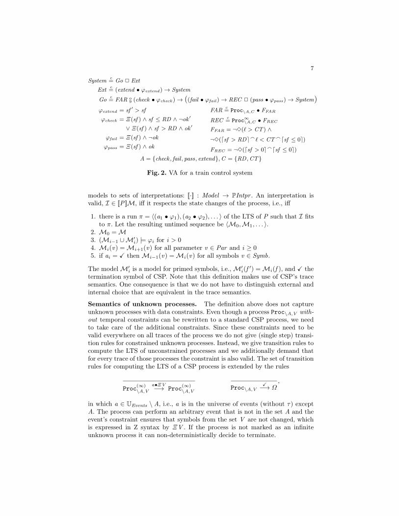
Symbolic execution of dCSP formulae. The rules of our calculus canbe found in Fig. 3. The rules (P1) up to (F4) are standard (cf. e.g., [11]) andresolve First-order formulae. Note that some of the rules like the cut rule (P3)are actually not necessary [11] but included to simplify proofs.
Our new proof rules are given in Fig. 3 from (C1) up to (U3). They symbol-ically unwind the CSP processes with data constraints and unknown processesalong their process structure. The rules correspond to the process operators in-troduced in Sect. 2. Rules that do not contain a sequent symbol can be appliedon both sides of a sequent. Generally, we have two rules for every operator be-cause we need different rules to cover the temporal case and the non-temporalcase. In the non-temporal case of the prefix operator (C4), we check that afterall executions of a → P the property δ holds. In the temporal case (C5), we needto check that ϕ is valid everywhere on all executions of a → P : we prove thatϕ holds everywhere on a → Skip and that [P ]ϕ holds after every executionof a. Rule (C6) splits up choice of processes into a conjunction of formulae. Thesequence rules (C7), (C8) are built-up identical to the prefix rules.
The rules (C9) and (C10) perform the symbolical execution of an event stepwith a corresponding data constraint: the event and the constraint are consumedand replaced by a new constraint representing the data change. Events are onlyrequired for synchronisation and can be reduced in this sequential situation. Inrule (C9), the constraint ψ of the event a contains primed and unprimed symbols,where the former relates to the post-state of the operation and the latter to thepre-state. After an execution of the data change in ψ the post-state of a systemvariable needs to coincide with the pre-state of this variable in δ. Hence, we showthat the constraint ψ, where every primed symbol v ′ is replaced by a fresh v0,implies δv0
v , i.e., δ, where every v is replaced by the corresponding v0.
10
`γ ` (P1)
`` γ (P2)
γ ` ` γ`
(P3) ϕ ` ϕ (P4) ` ϕ¬ϕ ` (P5)
ϕ `` ¬ϕ (P6)
ϕ,ψ `ϕ ∧ ψ ` (P7)
` ϕ ` ψ` ϕ ∧ ψ
(P8)
ϕ ` ψ `ϕ ∨ ψ `
(P9)
` ϕ,ψ` ϕ ∨ ψ (P10)
ψ ` ` ϕϕ⇒ ψ `
(P11)
ϕ ` ψ` ϕ⇒ ψ
(P12)
ϕ[t/x ], ∀ x : T • ϕ `∀ x : T • ϕ `
(F1)
` ϕ[y/x ]` ∀ x : T • ϕ (F2)
ϕ[y/x ] `∃ x : T • ϕ ` (F3)
` ϕ[t/x ],∃ x : T • ϕ` ∃ x : T • ϕ
(F4)
[P ]γ
[Q ]γ(C1)
δ
[Skip]δ(C2)
ϕ
[Skip]ϕ(C3)
[a][P ]δ
[a → P ]δ(C4)
[a]ϕ ∧ [a][P ]ϕ[a → P ]ϕ
(C5)
[P1]γ ∧ [P2]γ
[P1 2 P2]γ(C6)
[P1][P2]δ
[P1o9 P2]δ
(C7)([P1]ϕ) ∧ ([P1][P2]ϕ)
[P1o9 P2]ϕ
(C8)
ψv0v′ ⇒ δv0
v
[a • ψ]δ(C9)
ϕ ∧ [a • ψ]ϕ[a • ψ]ϕ
(C10)
[Q ]γ
[P ]γ(A1)
[P ]ϕ[P ]ϕ
(A2)ϕ ` [P ]δ
[Q ]ϕ ` [Q ][P ]δ(A3)
∆ ` ϕin(y), Γ ϕin(y),∀ x • (ϕin(x )⇒ [Qxy ]γ(x )) ` [F (Q)]γ(y)
∆ ` [P ]γ(y), Γ(I1)
ψ ` [Proc∞\A,V • F ]δ
(U1)
ϕ ` δ∆,ψ ` [Proc\A,V • F ]δ, Γ
(U2)ψ ` [Proc
(∞)
\A,V • F ]ϕ(U3)
In (F1) up to (F4), the term t is of type T and y is a fresh variable of type T notoccurring elsewhere. The process Q in (C1) is defined by Q c
= P . A formula ψv0v
denotes the replacement of variables v with fresh variables v0 for all v in ψ. In (A1),P and Q are equivalent CSP processes. In (I1), P is a recursive process P c
= F (P),γ(y), ϕin(y) are formulae over vectors of system variables containing no other systemvariables besides y . For side conditions of (U2), (U3) (that introduce ϕ) see Sect. 3.We abbreviate [a → Skip]γ by [a]γ and a • ϕ→ P by a → P if ϕ is of no relevance.
Fig. 3. Sequent calculus for CSP with data constraints
The rules (A1) up to (A3) are auxiliary rules for, e.g., -introduction andreplacement of equivalent processes. The latter is also used to cope with parallelcomposition: parallelism is replaced by an equivalent choice of processes.
Induction rules. In contrast to standard dynamic logic, dCSP expresses prop-erties over recursive processes. Hence, we provide induction rule (I1) here to allowreduction of recursion in CSP expressions. The rule is a variant of the Fixed-point Induction Rule of [26], but it is adapted to our needs. The premise of rule
11
(I1) consists of two proof commitments. First, we need to show that an initialcondition ϕin(y) holds in the current context. The intuition is that this formulaϕin holds after every cycle of the recursion and implies validity of the desiredformula γ for the next cycle and so on. The second commitment1 contains theinductive argument: assuming that ϕin implies that γ holds for an arbitraryprocess Q we must show that γ also holds for F (Q). The induction hypothesis ishereby given by ∀ x • (ϕin(x )⇒ [Qx
y ]γ(x )). It states that regardless of how ϕin
is instantiated with system variables x , if ϕin is valid for these x then [Qxy ]γ(x )
is also valid. We need to replace system variables y in Q by x because duringsymbolical execution of the process F (Q) new symbols are introduced.
Symbolic execution of constrained unknown processes. Finally, we needrules to handle unknown processes with temporal constraints. The idea is notto handle these constraints in our calculus directly. Instead, we call an external(semi-)decision procedure that checks if the constraints of the unknown processactually ensure properties by which the remaining proof can be completed. Thus,the rules we give here for handling of unknown process can be seen as oraclerules that access external techniques to reason over the temporal constraints.Hence, the rules directly reflect the semantics of constrained unknown processes.Rule (U1) is an axiom expressing the trivial fact that after termination of allnon-terminating processes everything is true. For the remaining two rules, theinteresting part is contained in the side-conditions. Rule (U2) is correct if forall modelsM withM |= ψ and all interpretations I ∈ [[Proc\A,V • F ]]M withterminating modelM the formula ϕ holds:M |= ϕ. This represents exactly thesemantics of [Proc\A,V • F ]ϕ. Further, δ has to follow from ϕ. The rule onlyapplies to terminating unknown processes (for the infinite case we cannot allowto consume the unknown process). Analogously, the side condition that must beproven for application of rule (U3) is that for all models M with M |= ψ andand all interpretations I ∈ [[Proc
(∞)\A,V • F ]]M the formula ϕ holds: I |= ϕ.
In this way, we can use an arbitrary proof method for the temporal logic ifit is possible to check the side-conditions of rules (U2) and (U3). By this means,our approach flexibly integrates arbitrary timed logics to formulate assumptionson unknown processes.
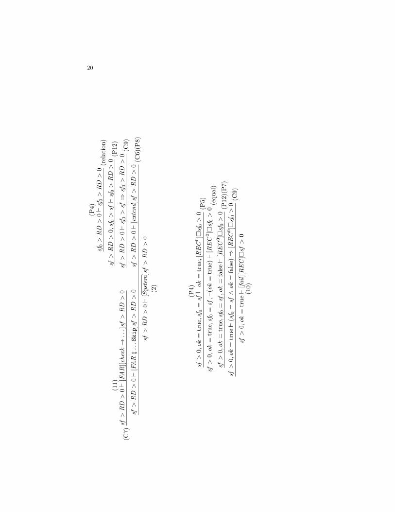
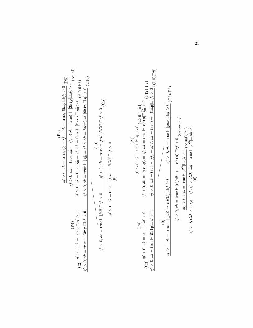
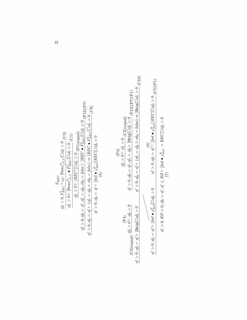
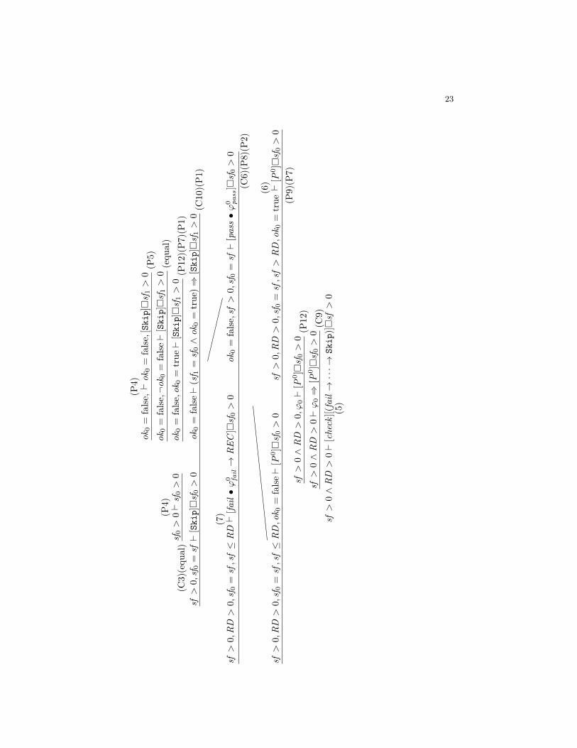
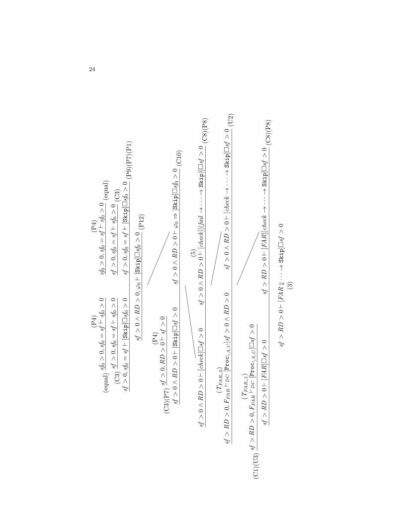
Example 2. The safety condition we want to prove for the architecture fromFig. 2 is that sf never reaches 0, in terms of dCSP sf > RD > 0 ` [System]sf >0 and we use our sequent calculus to prove its validity. To apply the proof rulesfor FAR and REC we need to verify the corresponding formulae FFAR andFREC via the standard model checking approach for COD and DC [21]. Wedemonstrate this for one branch of the proof tree:
1 The right formula of the premise (and likewise the premise of (U2)) does actuallynot contain the context formulae ∆ and Γ , that are implicit in the remaining rules.
12
sf > RD > 0(U3)` [Proc\A,C • FFAR]sf > 0 (C1)
sf > RD > 0 ` [FAR]sf > 0... (P8)
sf > RD > 0 ` [FAR]sf > 0 ∧ [FAR][check → · · · → Skip]sf > 0 (C8)sf > RD > 0 ` [FAR o
9 · · · → Skip]sf > 0
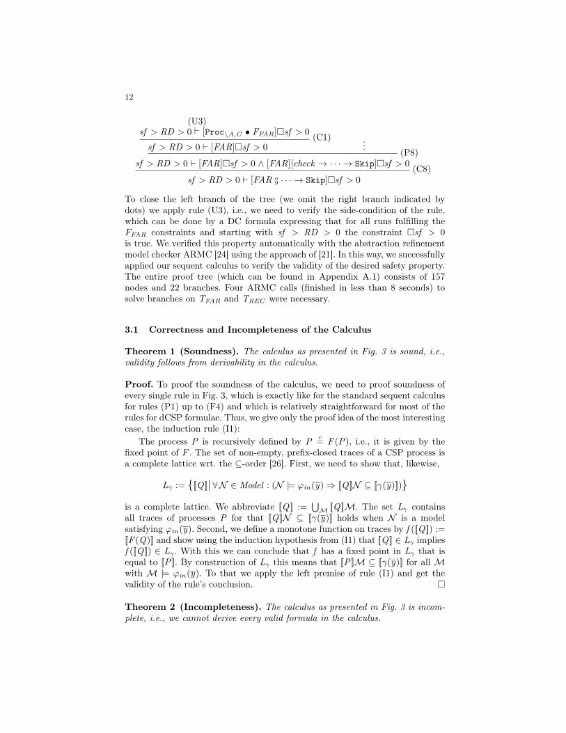
To close the left branch of the tree (we omit the right branch indicated bydots) we apply rule (U3), i.e., we need to verify the side-condition of the rule,which can be done by a DC formula expressing that for all runs fulfilling theFFAR constraints and starting with sf > RD > 0 the constraint sf > 0is true. We verified this property automatically with the abstraction refinementmodel checker ARMC [24] using the approach of [21]. In this way, we successfullyapplied our sequent calculus to verify the validity of the desired safety property.The entire proof tree (which can be found in Appendix A.1) consists of 157nodes and 22 branches. Four ARMC calls (finished in less than 8 seconds) tosolve branches on TFAR and TREC were necessary.
3.1 Correctness and Incompleteness of the Calculus
Theorem 1 (Soundness). The calculus as presented in Fig. 3 is sound, i.e.,validity follows from derivability in the calculus.
Proof. To proof the soundness of the calculus, we need to proof soundness ofevery single rule in Fig. 3, which is exactly like for the standard sequent calculusfor rules (P1) up to (F4) and which is relatively straightforward for most of therules for dCSP formulae. Thus, we give only the proof idea of the most interestingcase, the induction rule (I1):
The process P is recursively defined by P c= F (P), i.e., it is given by the
fixed point of F . The set of non-empty, prefix-closed traces of a CSP process isa complete lattice wrt. the ⊆-order [26]. First, we need to show that, likewise,
Lγ := [[Q ]]|∀N ∈ Model : (N |= ϕin(y)⇒ [[Q ]]N ⊆ [[γ(y)]])
is a complete lattice. We abbreviate [[Q ]] :=⋃M [[Q ]]M. The set Lγ contains
all traces of processes P for that [[Q ]]N ⊆ [[γ(y)]] holds when N is a modelsatisfying ϕin(y). Second, we define a monotone function on traces by f ([[Q ]]) :=[[F (Q)]] and show using the induction hypothesis from (I1) that [[Q ]] ∈ Lγ impliesf ([[Q ]]) ∈ Lγ . With this we can conclude that f has a fixed point in Lγ that isequal to [[P ]]. By construction of Lγ this means that [[P ]]M ⊆ [[γ(y)]] for all Mwith M |= ϕin(y). To that we apply the left premise of rule (I1) and get thevalidity of the rule’s conclusion.
Theorem 2 (Incompleteness). The calculus as presented in Fig. 3 is incom-plete, i.e., we cannot derive every valid formula in the calculus.
13
Proof. This is a direct consequence of the integration of an arbitrary temporallogic to constrain unknown processes. By this, we can choose an undecidablelogic like the full DC [33] and, thus, cannot resolve the constraints of thoseunknown processes in every case.
4 Refinement of Verification Architectures
We now show how a verified VA can be instantiated by specifications in thecombined formalism CSP-OZ-DC (COD) [15]. We recall that in our approachwe verify instantiation relations in two steps: assumptions on unknown processesare verified by customary verification approaches for the temporal logic and arefinement relation for the process structure needs to be established. Thus, wehere provide a rule to prove refinement by COD specifications syntactically.
CSP-OZ-DC [15,8] combines three well-investigated formalisms into a singlelanguage: it uses CSP to model the control flow of a system, Object-Z (OZ)[27] to specify data space and state changes via OZ schemata, and for defining(dense) real-time constraints, it applies DC counterexample traces. A key featureof CSP-OZ-DC is its separation of concerns, because every part, control flow,data space, and timing part can be specified on its own. Its semantic is given interms of interpretations [[cod ]] and it is compositional, thus, if one can establisha safety property for a single part of the specification the property automaticallyholds likewise for the entire specification. Note that the CSP part is defined interms of standard CSP (using trace semantics), i.e., it does not support unknownprocesses and it does not contain data (which is integrated via the OZ part).
Definition 3 (Refinement by COD specifications). Given a process P anda COD specification cod, a refinement of P by cod, written P v cod, is given iff
I | Minit ∈ Init(cod), I ∈ [[P ]](Minit) ⊇ [[cod ]], (6)
where Init(cod) is the set of all models that are valid initial models of cod.
This definition entails that the symbols, which are introduced in cod and thusare interpreted by the modelMinit , coincide with the symbols of the signatureΣ of a refined process P . Even though this definition does not impose explicitlyrestrictions on how symbols are declared and used in cod , it implicitly enforcesthe desired behaviour: whenever a symbol is changed in each execution of P thesymbol must be declared in cod .
We now give a proof rule that establishes a refinement relation between aCSP process with data and unknown processes (but without assumptions onunknowns, which are verified separately; cf. Sect. 1.2) and a COD specification:a COD specification refines a process if there is a syntactic matching betweenthem. The rule is not complete, i.e., not all valid refinements can be shownapplying the rule. But this is not our goal here, because in our applicationscenario concrete realisations are modelled with respect to a given VA and thuswe assume that the concrete model reflects the structure of the VA directly.
14
Definition 4 (Matching). Given a process P with unknown processes X1c=
Proc(∞)\A1,V1
, . . . ,Xnc= Proc
(∞)\An ,Vn
and a COD class cod, cod matches P if
1. The symbols of the signature Σ of P coincide with the symbols introducedin cod. That is, for Σ = (Sort ,Symb,Par ,Var) the types of cod correspondto the sorts Sort, state and message variables of cod to symbols from Symb,global constants to Par.
2. The CSP process of cod (the main process) structurally equals P except thatall unknown processes are replaced by implementing processes. We demandthat processes implementing Proc∞ do not contain the Skip process.
3. For every process Pi implementing Proc\A,V we demand that (1) the for-bidden events from A are respected, i.e., alphabet(Pi)∩Ai = ∅, and (2) thefunction symbols from V are not changed, i.e., given an operation a ∈alphabet(Pi) with a delta list2 ∆(s1, . . . , sn) it holds si 6∈ V for i ∈ 1..n.
4. For every occurrence of an event a • ϕ in P, where ϕ has function symbolss1, . . . , sm and primed function symbols u ′1, . . . , u ′l , there is a schema
com a = [∆(u1, . . . , ul); x1 : S1; . . . ; xn : Sn | ϕ]
in cod and the function symbols are declared in cod. The variables x1 to xnare the message variables of channel a used for communications.
The last condition also implies that for events a • ϕ1 and a • ϕ2, ϕ1 and ϕ2 arealways equal, because different definitions of com a are not allowed in COD.
Theorem 3 (Proof rule: Matching implies refinement). Let P be a CSPprocess and let cod a COD specification such that cod matches P. Then, P v cod.
Proof. We give the proof idea here. The COD specification cod and the processP have the same semantical domain, timed interpretations. State changes areexecuted by constraints alongside the occurrence of events in both cases. Byconstruction of the refinement rule, all constraints (and by this all state changes)coincide and hence we only need to prove that all traces of events performed bycod , which are traces of its main process, are also valid traces of the process P .We show this by proving that P down-simulates the process of cod , that is, thereis a relation on processes s.t. for all R,S ,S
R S and S a=⇒ S implies that there is an R with R a
=⇒ R and R S .
It is then a standard result [13] that we can conclude from P main that mainis a refinement of P and by this P v cod .
The notion of refinement introduced here is rather restricted because thesymbols and the constraints of COD specification and VA process have to coin-cide. It is straightforward to extend the definitions as well as the refinement ruleto arbitrary refinement relations on the symbols of COD specification and VAprocess by which more sophisticated connections are possible. E.g., an abstractdata type like a list over arbitrary objects can be mapped by the refinementrelation to a concrete list of integer values.2 Operations in COD carry a delta list ∆(s1, . . . , sn) of symbols that can be changed.
15
Example 3. In our running example, we proved the correctness of an instanti-ation of the VA from Fig. 2. This instantiation was given as a concrete CODmodel (see Appendix A.2), for that direct verification was not possible (timeoutafter 80h) due to its complexity with 17 real-valued variables and clocks, over300 program locations, and 17000 transitions. Since the model is a refinementof the VA, which can be syntactically checked, we only needed to verify thelocal DC formulae FFAR and FREC to conclude the safety of the entire system(cf. Sect. 1.2). This was done automatically with ARMC in 7h (FFAR) and 4m(FREC ), respectively.
5 Conclusion
The main theme in this work was to uniformly integrate verification techniquesin a formal framework to allow compositional verification of real-time systems:VAs combine CSP with data and additional real-time constraints to define be-havioural protocols for classes of systems. Our new sequent-style proof calculusallows us to verify VAs by a combination of proof rule based reasoning and asuited verification technique for timed constraints. As a proof of concept, we con-sidered instantiations of VAs by COD specifications and gave a syntactic proofrule to establish refinement relations. We were able to verify a COD-specifiedtrain control system that is too complex to be verified without further decom-position techniques. However, the basic ideas of our VA approach carry over toother formalisms. Particularly, our new CSP dialect is not bound to COD butcan be used with other CSP-based combined formalisms, e.g., [32,29], for whichsyntactic refinement rules can be defined similarly to the rule from Sect. 4.
Even though we do not have tool support for the proof calculus from Sect. 3,the VA approach is dedicated to automated verification and there are promisingresults in automated verification for similar calculi [23].
A question that we have not investigated in this paper is the completenessof the VA approach: can appropriate assumptions be found for every possibleinstantiation of an architecture? The answer depends on the languages used forthe assumptions and the instantiations. Present results for COD and DC suggestthat this is actually the case because every COD instantiation can be translatedinto an equivalent DC expression.
Additionally, we have first achievements in extending the logic and the cal-culus to reason about more complex real-time properties like DC traces.
Acknowledgements. The author thanks Ernst-Rüdiger Olderog and AndersP. Ravn for helpful comments.
References
1. Abrial, J.R., Mussat, L.: Introducing dynamic constraints in B. In: Bert, D. (ed.)B. LNCS, vol. 1393, pp. 83–128. Springer, Heidelberg (1998)
2. Butler, M.J.: A CSP Approach To Action Systems. Ph.D. thesis, University ofOxford (1992)
16
3. Damm, W., Hungar, H., Olderog, E.R.: Verification of cooperating traffic agents.Int. J. Control. 79(5), 395 – 421 (2006)
4. de Roever, W.P. et al: Concurrency Verification: Introduction to Compositionaland Noncompositional Methods. Cambridge University Press, Cambridge (2001)
5. D’Errico, L., Loreti, M.: Assume-Guarantee Verification of Concurrent Systems.In: Field, J., Vasconcelos, V.T. (eds.) COORDINATION 2009. LNCS, vol. 5521,pp. 288–305. Springer, Heidelberg (2009)
6. Dong, J.S., Hao, P., Qin, S., Sun, J., Yi, W.: Timed patterns: TCOZ to timedautomata. In: Davies, J., Schulte, W., Barnett, M. (eds.) ICFEM 2004. LNCS, vol.3308, pp. 483–498. Springer, Heidelberg (2004)
7. ERTMS User Group, UNISIG: ERTMS/ETCS System requirements specification.http://www.aeif.org/ccm/default.asp (2002), version 2.2.2
8. Faber, J., Jacobs, S., Sofronie-Stokkermans, V.: Verifying CSP-OZ-DC specifica-tions with complex data types and timing parameters. In: Davies, J., Gibbons, J.(eds.) IFM 2007. LNCS, vol. 4591, pp. 233–252. Springer, Heidelberg (2007)
9. Faber, J.: Verification Architectures: Compositional reasoning for real-time sys-tems. In: Méry, D., Merz, S. (eds.) IFM 2010. LNCS, vol. 6396, pp. 136–151.Springer, Heidelberg (2010)
10. Fischer, C.: Combination and Implementation of Processes and Data: from CSP-OZ to Java. Ph.D. thesis, University of Oldenburg (2000)
11. G. Gentzen: Untersuchungen über das logisches Schließen. MathematischeZeitschrift 1, 176–210 (1935)
12. Harel, D., Kozen, D., Tiuryn, J.: Dynamic Logic. MIT Press, Cambridge (2000)13. He, J.: Process simulation and refinement. Form. Asp. Comput. 1(3), 229–241
(1989)14. Hoare, C.A.R.: Communicating Sequential Processes. Prentice Hall International,
Englewood Cliffs (1985)15. Hoenicke, J.: Combination of Processes, Data, and Time. Ph.D. thesis, University
of Oldenburg (2006)16. Klebanov, V., Rümmer, P., Schlager, S., Schmitt, P.H.: Verification of JCSP pro-
grams. In: Broenink, J.F., Roebbers, H.W., Sunter, J.P.E., Welch, P.H., Wood,D.C. (eds.) CPA. CSES, vol. 63, pp. 203–218. IOS Press, Amsterdam (2005)
17. Knudsen, J., Ravn, A.P., Skou, A.: Design verification patterns. In: Jones, C.B.,Liu, Z., Woodcock, J. (eds.) Formal Methods and Hybrid Real-Time Systems.LNCS, vol. 4700, pp. 399–413. Springer, Heidelberg (2007)
18. Larsen, K.G., Xinxin, L.: Compositionality through an operational semantics ofcontexts. J. Log. Comput. 1(6), 761–795 (1991)
19. Mahony, B.P., Dong, J.S.: Blending object-Z and timed CSP: An introduction toTCOZ. In: ICSE. pp. 95–104 (1998)
20. Metzler, B., Wehrheim, H., Wonisch, D.: Decomposition for compositional verifi-cation. In: Liu, S., Maibaum, T.S.E., Araki, K. (eds.) ICFEM 2008. LNCS, vol.5256, pp. 105–125. Springer, Heidelberg (2008)
21. Meyer, R., Faber, J., Hoenicke, J., Rybalchenko, A.: Model checking duration cal-culus: A practical approach. Form. Asp. Comput. 20(4–5), 481–505 (2008)
22. Platzer, A.: A temporal dynamic logic for verifying hybrid system invariants. In:Artemov, Nerode (eds.) LFCS 2007. LNCS, vol. 4514, pp. 457–471. Springer, Hei-delberg (2007)
23. Platzer, A., Quesel, J.D.: Logical verification and systematic parametric analysisin train control. In: Egerstedt, M., Mishra, B. (eds.) HSCC 2008. LNCS, vol. 4981,pp. 646–649. Springer, Heidelberg (2008)
17
24. Podelski, A., Rybalchenko, A.: ARMC: The logical choice for software model check-ing with abstraction refinement. In: Hanus, M. (ed.) PADL 2007. LNCS, vol. 4354,pp. 245–259. Springer, Heidelberg (2007)
25. RAISE Language Group: The RAISE Specification Language. BCS PractitionerSeries, Prentice Hall International, Englewood Cliffs (1992)
26. Roscoe, A.: Theory and Practice of Concurrency. Prentice Hall International, En-glewood Cliffs (1998)
27. Smith, G.: An integration of real-time object-Z and CSP for specifying concurrentreal-time systems. In: Butler, M.J., Petre, L., Sere, K. (eds.) IFM 2002. LNCS, vol.2335, pp. 267–285. Springer, Heidelberg (2002)
28. Sühl, C.: An overview of the integrated formalism RT-Z. Form. Asp. Comput.13(2), 94–110 (2002)
29. Sun, J., Liu, Y., Dong, J.S.: Model checking CSP revisited: Introducing a processanalysis toolkit. In: ISoLA 2008. CCIS, vol. 17, pp. 307–322. Springer, Heidelberg(2008)
30. Taibi, T.: Design Pattern Formalization Techniques. IGI Publishing (2007)31. Wehrheim, H.: Behavioural subtyping in object-oriented specification formalisms.
Habilitation, University of Oldenburg (2002)32. Woodcock, J.C.P., Cavalcanti, A.L.C.: A concurrent language for refinement. In:
Butterfield, A., Pahl, C. (eds.) IWFM 2001. BCS Elec. Works. in Computing (2001)33. Zhou, C., Hansen, M.R.: Duration Calculus. Springer, Heidelberg (2004)34. Zhou, C., Hoare, C.A.R., Ravn, A.P.: A calculus of durations. Information Pro-
cessing Letters 40(5), 269–276 (1991)
18
A Appendix
This appendix contains some additional material to further illustrate the traincontrol system of our running example: the full proof tree of Example 2 and theCSP-OZ-DC instantiation of Example 3.
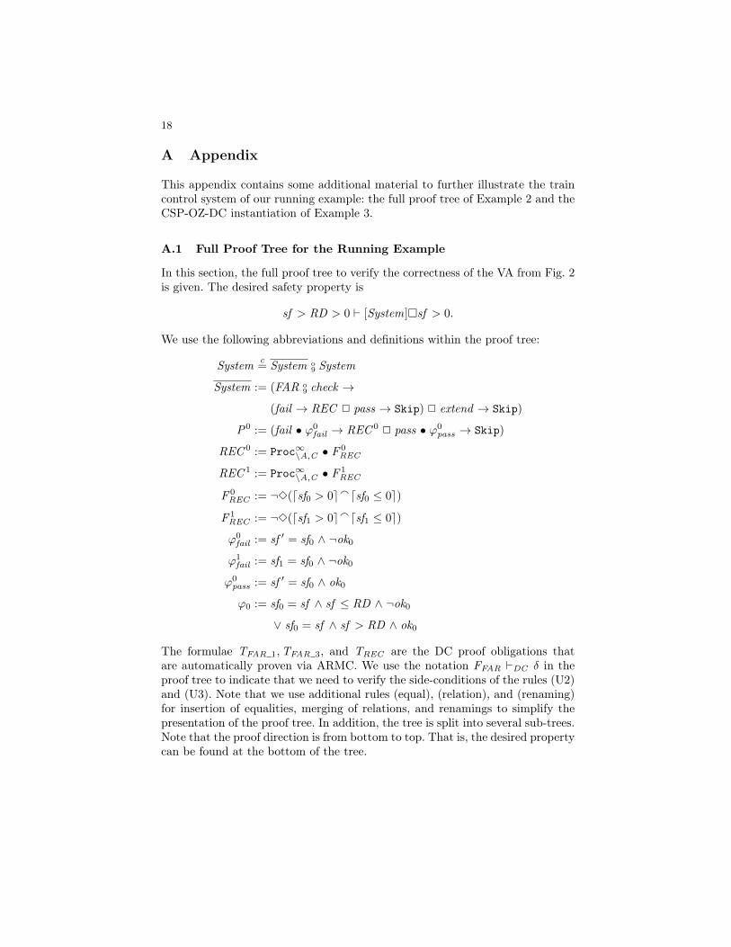
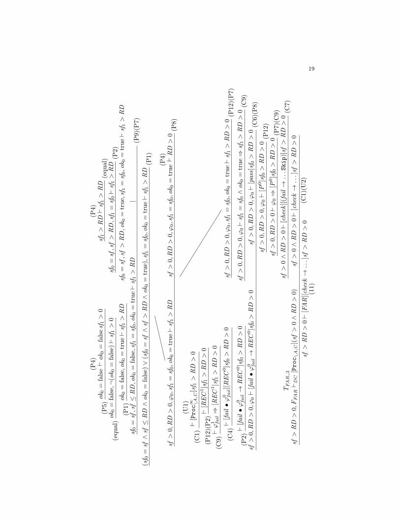
A.1 Full Proof Tree for the Running Example
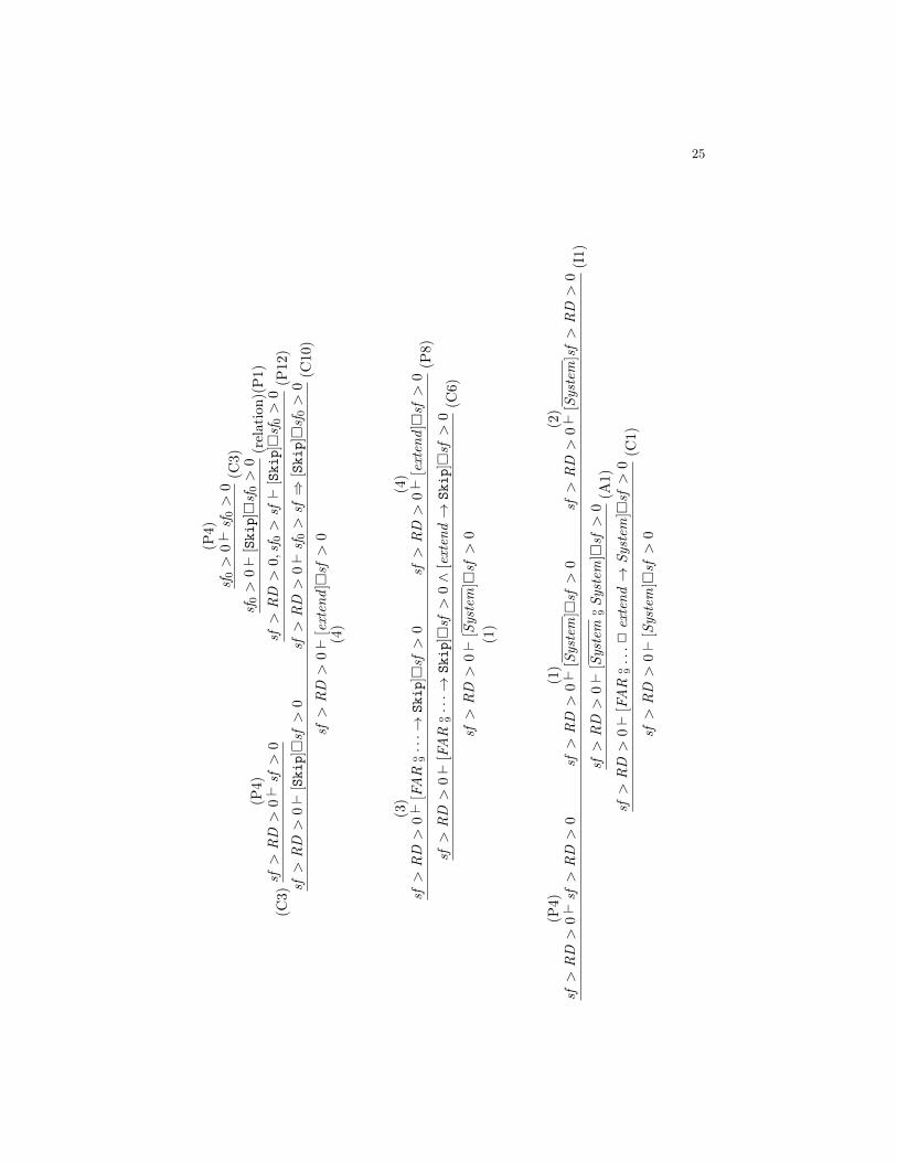
In this section, the full proof tree to verify the correctness of the VA from Fig. 2is given. The desired safety property is
sf > RD > 0 ` [System]sf > 0.
We use the following abbreviations and definitions within the proof tree:
System c= System o
9 System
System := (FAR o9 check →
(fail → REC 2 pass → Skip) 2 extend → Skip)
P0 := (fail • ϕ0fail → REC 0 2 pass • ϕ0
pass → Skip)
REC 0 := Proc∞\A,C • F0REC
REC 1 := Proc∞\A,C • F1REC
F 0REC := ¬3(dsf0 > 0eadsf0 ≤ 0e)
F 1REC := ¬3(dsf1 > 0eadsf1 ≤ 0e)
ϕ0fail := sf ′ = sf0 ∧ ¬ok0
ϕ1fail := sf1 = sf0 ∧ ¬ok0
ϕ0pass := sf ′ = sf0 ∧ ok0
ϕ0 := sf0 = sf ∧ sf ≤ RD ∧ ¬ok0∨ sf0 = sf ∧ sf > RD ∧ ok0
The formulae TFAR 1,TFAR 3, and TREC are the DC proof obligations thatare automatically proven via ARMC. We use the notation FFAR `DC δ in theproof tree to indicate that we need to verify the side-conditions of the rules (U2)and (U3). Note that we use additional rules (equal), (relation), and (renaming)for insertion of equalities, merging of relations, and renamings to simplify thepresentation of the proof tree. In addition, the tree is split into several sub-trees.Note that the proof direction is from bottom to top. That is, the desired propertycan be found at the bottom of the tree.
19
(P5)
ok0=
false(P
4) `ok
0=
falsesf 1>
0sf
1>
RD(P
4) `sf
1>
RD
(equ
al)
(equ
al)ok
0=
false,¬(
ok0=
false)`sf
1>
0sf
0=
sf,sf>
RD,sf 1
=sf
0`sf
1>
RD
(P2)
(P1)
ok0=
false,ok
0=
true`sf
1>
RD
sf0=
sf,sf>
RD,ok 0
=true,sf 1
=sf
0,ok 0
=true`sf
1>
RD
sf0=
sf,sf≤
RD,ok 0
=false,sf
1=
sf0,ok 0
=true`sf
1>
RD
(P9)(P
7)(sf 0
=sf∧sf≤
RD∧ok
0=
false)∨(sf 0
=sf∧sf>
RD∧ok
0=
true),sf
1=
sf0,ok 0
=true`sf
1>
RD
(P1)
sf>
0,RD>
0,ϕ
0,sf 1
=sf
0,ok 0
=true`sf
1>
RD
sf>
0,R
D>
0,ϕ0,sf 1
=sf
0,ok 0
=true(P
4) `RD>
0(P
8)
(C1)
(U1)
`[Proc∞ \A,C]sf 1>
RD>
0
(P12)(P2)`[REC
1]sf 1>
RD>
0
(C9)`ϕ1 fa
il⇒
[REC
1]sf 1>
RD>
0
(C4)`[fa
il•ϕ0 fa
il][REC
0]sf 0>
RD>
0sf>
0,RD>
0,ϕ0,sf 1
=sf
0,ok 0
=true`sf
1>
RD>
0(P
12)(P7)
(P2)`[fa
il•ϕ0 fa
il→
REC
0]sf 0>
RD>
0sf>
0,RD>
0,ϕ
0`sf
1=
sf0∧ok
0=
true⇒
sf1>
RD>
0(C
9)sf>
0,R
D>
0,ϕ0`[fa
il•ϕ0 fa
il→
REC
0]sf 0>
RD>
0sf>
0,R
D>
0,ϕ0`[pass]sf
0>
RD>
0(C
6)(P
8)sf>
0,RD>
0,ϕ
0`[P
0]sf 0>
RD>
0(P
12)
sf>
0,R
D>
0`ϕ0⇒
[P0]sf 0>
RD>
0(P
7)(C
9)sf>
0∧RD>
0`[check
][(fail→...Skip)]sf>
RD>
0(C
7)sf>
RD>
0,F
FA
RTFA
R3
` DC
[Proc\A,C](sf>
0∧RD>
0)
sf>
0∧RD>
0`[check→...]sf>
RD>
0
(C1)(U
2)sf>
RD>
0`[FAR][check→...]sf>
RD>
0(11)
20
sf0>
RD>
0(P4) `sf
0>
RD>
0(relation)
sf>
RD>
0,sf 0>
sf`sf
0>
RD>
0(P
12)
(C7)
sf>
RD>
0(11) `[FAR][check→...]sf>
RD>
0sf>
RD>
0`sf
0>
sf⇒
sf0>
RD>
0(C
9)sf>
RD>
0`[FAR
o 9...Skip]sf>
RD>
0sf>
RD>
0`[extend]sf>
RD>
0(C
6)(P
8)sf>
RD>
0`[System]sf>
RD>
0
(2)
sf>
0,ok
=true,sf 0
=sf(P
4) `ok
=true,[REC
0]
sf0>
0(P
5)sf>
0,ok
=true,sf 0
=sf,¬
(ok=
true)`[REC
0]
sf0>
0(equ
al)
sf>
0,ok=
true,sf 0
=sf,ok=
false`[REC
0]
sf0>
0(P
12)(P7)
sf>
0,ok
=true`(sf 0
=sf∧ok
=false)⇒
[REC
0]
sf0>
0(C
9)sf>
0,ok=
true`[fa
il][REC]
sf>
0(10)
21
sf>
0,ok
=true,sf 0
=sf(P
4) `ok
=true,[Skip]
sf0>
0(P
5)sf>
0,ok=
true,sf 0
=sf,¬
(ok=
true),`[Skip]
sf0>
0(equ
al)
(C3)
sf>
0,ok=
true,(P
4) `sf>
0sf>
0,ok
=true,sf 0
=sf,ok=
false`[Skip]
sf0>
0(P
12)(P7)
sf>
0,ok
=true`[Skip]
sf>
0sf>
0,ok
=true`(sf 0
=sf∧ok
=false)⇒
[Skip]
sf0>
0(C
10)
sf>
0,ok=
true`[fa
il]
sf>
0sf>
0,ok=
true(10) `[fa
il][REC]
sf>
0(C
5)
sf>
0,ok=
true`[fa
il→
REC]
sf>
0(9)
sf0>
0,ok
=true(P
4) `sf
0>
0(C
3)(equ
al)
(C3)
sf>
0,ok
=true(P
4) `sf>
0sf>
0,ok=
true,sf 0
=sf,ok=
true`[Skip]
sf0>
0(P
12)(P7)
sf>
0,ok
=true`[Skip]
sf>
0sf>
0,ok=
true`(sf 0
=sf∧ok
=true)⇒
[Skip]
sf0>
0(C
10)(P8)
sf>
0,ok
=true
(9) `[(fail→
REC)]sf>
0sf>
0,ok
=true`[pass]sf>
0(C
6)(P
8)
sf>
0,ok=
true`[((fail→...Skip)]sf>
0(renam
ing)
sf0>
0,ok
0=
true`[P
0]
sf0>
0(equ
al)(P1)
sf>
0,RD>
0,sf 0
=sf,sf>
RD,ok 0
=true`[P
0]
sf0>
0(6)
22
sf1>
0,F
1 REC
TREC
` DC
[Proc∞ \A,C]
sf1>
0(U
3)sf
1>
0`[Proc∞ \A,C•F
1 REC]
sf1>
0(C
1)sf
1>
0`[REC
1]
sf1>
0(P
1)(equ
al)
sf>
0,sf
0=
sf,sf 1
=sf
0,ok 0
=false`[REC•F
1 REC]
sf1>
0(P
12)(P7)
sf>
0,sf 0
=sf`(sf 1
=sf
0∧ok
0=
false)⇒
[REC•F
1 REC]
sf1>
0(C
9)sf>
0,sf
0=
sf`[fa
il•ϕ0 fa
il][REC]
sf0>
0(8)
sf1>
0(P4) `sf
1>
0(C
3)(equ
al)
(C3)(equ
al)sf
0>
0(P4) `sf
0>
0sf>
0,sf
0=
sf,sf 1
=sf
0`[Skip]
sf1>
0(P
12)(P7)(P
1)sf>
0,sf
0=
sf`[Skip]
sf0>
0sf>
0,sf
0=
sf`(sf 1
=sf
0∧ok
0=
false)⇒
[Skip]
sf1>
0(C
10)
sf>
0,sf 0
=sf`[fa
il•ϕ0 fa
il]
sf0>
0sf>
0,sf
0=
sf(8) `[fa
il•ϕ0 fa
il][REC]
sf0>
0(C
5)(P
1)
sf>
0,RD>
0,sf 0
=sf,sf≤
RD`[fa
il•ϕ0 fa
il→
REC]
sf0>
0(7)
23
ok0=
false,(P
4) `ok
0=
false,[Skip]
sf1>
0(P
5)ok
0=
false,¬o
k 0=
false`[Skip]
sf1>
0(equ
al)
(C3)(equ
al)sf
0>
0(P4) `sf
0>
0ok
0=
false,ok
0=
true`[Skip]
sf1>
0(P
12)(P7)(P
1)sf>
0,sf 0
=sf`[Skip]
sf0>
0ok
0=
false`(sf 1
=sf
0∧ok
0=
true)⇒
[Skip]
sf1>
0(C
10)(P1)
sf>
0,RD>
0,sf
0=
sf,sf≤
RD(7) `[fa
il•ϕ0 fa
il→
REC]
sf0>
0ok
0=
false,sf>
0,sf
0=
sf`[pass•ϕ0 pa
ss]
sf0>
0
(C6)(P
8)(P
2)
sf>
0,RD>
0,sf
0=
sf,sf≤
RD,ok 0
=false`[P
0]
sf0>
0sf>
0,RD>
0,sf 0
=sf,sf>
RD,ok 0
=true
(6) `[P
0]
sf0>
0
(P9)(P
7)sf>
0∧RD>
0,ϕ0`[P
0]
sf0>
0(P
12)
sf>
0∧RD>
0`ϕ0⇒
[P0]
sf0>
0(C
9)sf>
0∧RD>
0`[check
][(fail→···→
Skip)]sf>
0(5)
24
(equ
al)sf
0>
0,sf
0=
sf(P4) `sf
0>
0sf
0>
0,sf 0
=sf(P
4) `sf
0>
0(equ
al)
(C3)
sf>
0,sf
0=
sf`sf
0>
0sf>
0,sf
0=
sf`sf
0>
0(C
3)sf>
0,sf
0=
sf`[Skip]
sf0>
0sf>
0,sf
0=
sf`[Skip]
sf0>
0(P
9)(P
7)(P
1)sf>
0∧RD>
0,ϕ0`[Skip]
sf0>
0(P
12)
(C3)(P
7)sf>
0,R
D>
0(P4) `sf>
0
sf>
0∧RD>
0`[Skip]
sf>
0sf>
0∧RD>
0`ϕ0⇒
[Skip]
sf0>
0(C
10)
sf>
0∧RD>
0`[check
]sf>
0sf>
0∧RD>
0(5) `[check
][(fail→···→
Skip)]sf>
0(C
8)(P
8)
sf>
RD>
0,F
FA
R(TFA
R3)
` DC
[Proc\A,C]sf>
0∧RD>
0sf>
0∧RD>
0`[check→···→
Skip]
sf>
0(U
2)
(C1)(U
3)sf>
RD>
0,F
FA
R(TFA
R1)
` DC
[Proc\A,C]
sf>
0
sf>
RD>
0`[FAR]
sf>
0sf>
RD>
0`[FAR][check→···→
Skip]
sf>
0(C
8)(P
8)
sf>
RD>
0`[FAR
o 9···→
Skip]
sf>
0
(3)
25
sf0>
0(P4) `sf
0>
0(C
3)sf
0>
0`[Skip]
sf0>
0(relation)(P
1)
(C3)
sf>
RD>
0(P4) `sf>
0sf>
RD>
0,sf 0>
sf`[Skip]
sf0>
0(P
12)
sf>
RD>
0`[Skip]
sf>
0sf>
RD>
0`sf
0>
sf⇒
[Skip]
sf0>
0(C
10)
sf>
RD>
0`[extend]sf>
0(4)
sf>
RD>
0(3) `[FAR
o 9···→
Skip]
sf>
0sf>
RD>
0(4) `[extend]sf>
0(P
8)sf>
RD>
0`[FAR
o 9···→
Skip]
sf>
0∧[extend→
Skip]
sf>
0(C
6)sf>
RD>
0`[System]
sf>
0
(1)
sf>
RD>
0(P4) `sf>
RD>
0sf>
RD>
0(1) `[System]
sf>
0sf>
RD>
0(2) `[System]sf>
RD>
0(I1)
sf>
RD>
0`[System
o 9Sy
stem
]sf>
0(A
1)sf>
RD>
0`[FAR
o 9...2
extend→
System
]sf>
0(C
1)sf>
RD>
0`[System]
sf>
0
26
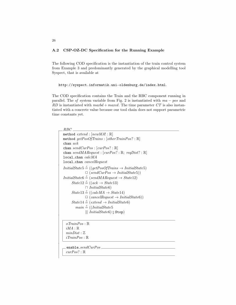
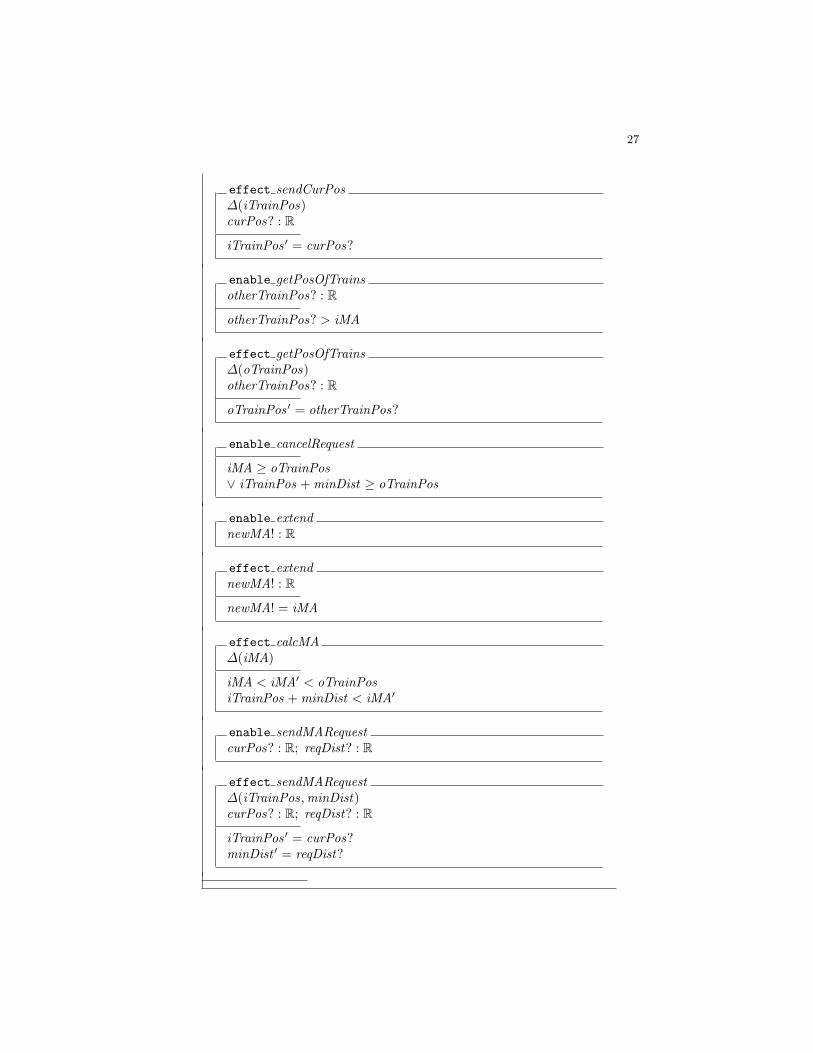
A.2 CSP-OZ-DC Specification for the Running Example
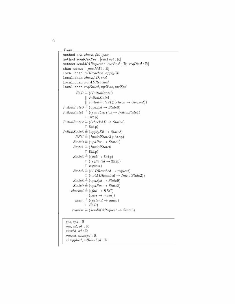
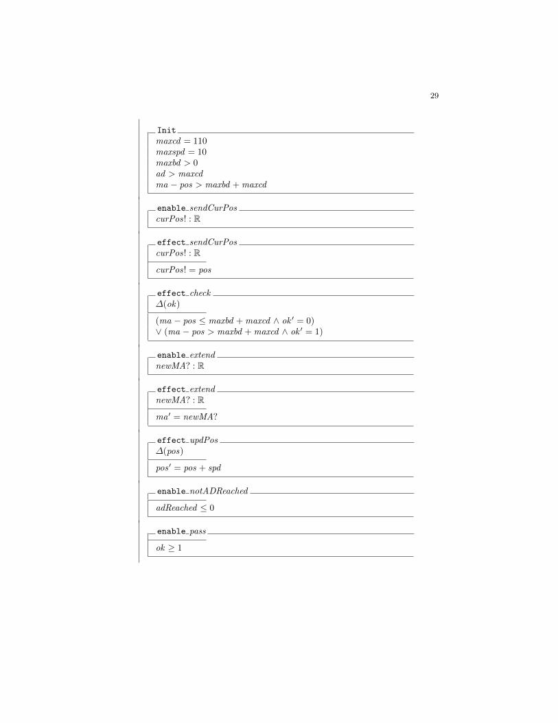
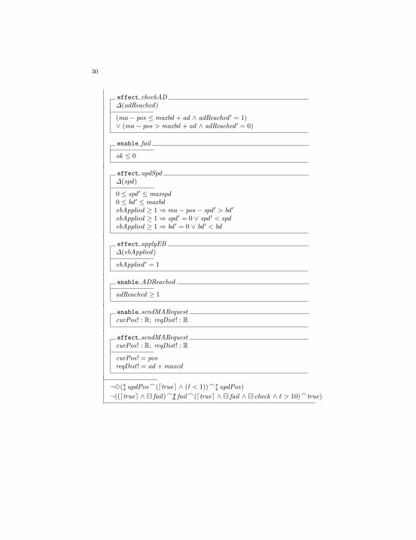
The following COD specification is the instantiation of the train control systemfrom Example 3 and predominantly generated by the graphical modelling toolSyspect, that is available at
http://syspect.informatik.uni-oldenburg.de/index.html.
The COD specification contains the Train and the RBC component running inparallel. The sf system variable from Fig. 2 is instantiated with ma − pos andRD is instantiated with maxbd +maxcd . The time parameter CT is also instan-tiated with a concrete value because our tool chain does not support parametrictime constants yet.
RBCmethod extend : [newMA! : R]method getPosOfTrains : [otherTrainPos? : R]chan ackchan sendCurPos : [curPos? : R]chan sendMARequest : [curPos? : R; reqDist? : R]local chan calcMAlocal chan cancelRequest
InitialState5 c= ((getPosOfTrains → InitialState5)2 (sendCurPos → InitialState5))
InitialState6 c= (sendMARequest → State12)
State12 c= ((ack → State13)u InitialState6)
State13 c= ((calcMA→ State14)2 (cancelRequest → InitialState6))
State14 c= (extend → InitialState6)
main c= ((InitialState5‖| InitialState6) o
9 Stop)
oTrainPos : RiMA : RminDist : ZiTrainPos : R
enable sendCurPoscurPos? : R
27
effect sendCurPos∆(iTrainPos)curPos? : R
iTrainPos ′ = curPos?
enable getPosOfTrainsotherTrainPos? : R
otherTrainPos? > iMA
effect getPosOfTrains∆(oTrainPos)otherTrainPos? : R
oTrainPos ′ = otherTrainPos?
enable cancelRequest
iMA ≥ oTrainPos∨ iTrainPos +minDist ≥ oTrainPos
enable extendnewMA! : R
effect extendnewMA! : R
newMA! = iMA
effect calcMA∆(iMA)
iMA < iMA′ < oTrainPosiTrainPos +minDist < iMA′
enable sendMARequestcurPos? : R; reqDist? : R
effect sendMARequest∆(iTrainPos,minDist)curPos? : R; reqDist? : R
iTrainPos ′ = curPos?minDist ′ = reqDist?
28
Trainmethod ack , check , fail , passmethod sendCurPos : [curPos! : R]method sendMARequest : [curPos! : R; reqDist ! : R]chan extend : [newMA? : R]local chan ADReached , applyEBlocal chan checkAD , endlocal chan notADReachedlocal chan reqFailed , updPos, updSpd
FAR c= ((InitialState0‖| InitialState1‖| InitialState2) o
9 (check → checked))InitialState0 c
= (updSpd → State0)InitialState1 c
= ((sendCurPos → InitialState1)u Skip)
InitialState2 c= ((checkAD → State5)u Skip)
InitialState3 c= (applyEB → State8)
REC c= (InitialState3 o
9 Stop)
State0 c= (updPos → State1)
State1 c= (InitialState0u Skip)
State3 c= ((ack → Skip)u (reqFailed → Skip)u request)
State5 c= ((ADReached → request)2 (notADReached → InitialState2))
State8 c= (updSpd → State9)
State9 c= (updPos → State8)
checked c= ((fail → REC )2 (pass → main))
main c= ((extend → main)u FAR)
request c= (sendMARequest → State3)
pos, spd : Rma, ad , ok : Rmaxbd , bd : Rmaxcd ,maxspd : RebApplied , adReached : R
29
Initmaxcd = 110maxspd = 10maxbd > 0ad > maxcdma − pos > maxbd +maxcd
enable sendCurPoscurPos! : R
effect sendCurPoscurPos! : R
curPos! = pos
effect check∆(ok)
(ma − pos ≤ maxbd +maxcd ∧ ok ′ = 0)∨ (ma − pos > maxbd +maxcd ∧ ok ′ = 1)
enable extendnewMA? : R
effect extendnewMA? : R
ma ′ = newMA?
effect updPos∆(pos)
pos ′ = pos + spd
enable notADReached
adReached ≤ 0
enable pass
ok ≥ 1
30
effect checkAD∆(adReached)
(ma − pos ≤ maxbd + ad ∧ adReached ′ = 1)∨ (ma − pos > maxbd + ad ∧ adReached ′ = 0)
enable fail
ok ≤ 0
effect updSpd∆(spd)
0 ≤ spd ′ ≤ maxspd0 ≤ bd ′ ≤ maxbdebApplied ≥ 1⇒ ma − pos − spd ′ > bd ′ebApplied ≥ 1⇒ spd ′ = 0 ∨ spd ′ < spdebApplied ≥ 1⇒ bd ′ = 0 ∨ bd ′ < bd
effect applyEB∆(ebApplied)
ebApplied ′ = 1
enable ADReached
adReached ≥ 1
enable sendMARequestcurPos! : R; reqDist ! : R
effect sendMARequestcurPos! : R; reqDist ! : R
curPos! = posreqDist ! = ad +maxcd
¬3(l updPosa(dtruee ∧ (` < 1))al updPos)¬((dtruee ∧ fail)a6 l faila(dtruee ∧ fail ∧ check ∧ ` > 10)a true)