Embed Size (px)
Citation preview
Verification Manual GE
Written by:
The SoilVision Systems Ltd. Team
Last Updated: Thursday, March 22, 2018
SoilVision Systems Ltd. Saskatoon, Saskatchewan, Canada

Software License The software described in this manual is furnished under a license agreement. The software may be used or copied only in accordance with the terms of the agreement.
Software Support Support for the software is furnished under the terms of a support agreement.
Copyright Information contained within this Verification Manual is copyrighted and all rights are reserved by SoilVision Systems Ltd. The SVFLUX software is a proprietary product and trade secret of SoilVision Systems. The Verification Manual may be reproduced or copied in whole or in part by the software licensee for use with running the software. The Verification Manual may not be reproduced or copied in any form or by any means for the purpose of selling the copies.
Disclaimer of Warranty SoilVision Systems Ltd. reserves the right to make periodic modifications of this product without obligation to notify any person of such revision. SoilVision Systems Ltd. does not guarantee,
warrant, or make any representation regarding the use of, or the results of, the programs in terms of correctness, accuracy, reliability, currentness, or otherwise; the user is expected to make the final evaluation in the context of his (her) own models.
Trademarks © 2015 - 2018 SoilVision Systems Ltd. All rights reserved. SoilVision.com, SoilVision logo, and SVSLOPE are registered trademarks of SoilVision Systems Ltd. SVOFFICE, SVOFFICE 5/GE, SVOFFICE 5/GT, SVOFFICE 5/WR, SVSOILS, SVFLUX, SVSOLID, SVCHEM, SVAIR, SVHEAT and SVDESIGNER are trademarks of SoilVision Systems Ltd. FlexPDE is a registered trademark of PDE Solutions Inc. FEHM is used under license from Los Alamos National Laboratories.
Copyright 2018
by
SoilVision Systems Ltd.
Saskatoon, Saskatchewan, Canada
ALL RIGHTS RESERVED
Printed in Canada
SoilVision Systems Ltd. Table of Contents 3 of 61
1 INTRODUCTION .............................................................................................................. 4
2 ONE-DIMENSIONAL SEEPAGE ..................................................................................... 5
2.1 TRANSIENT-STATE .................................................................................................................. 5 2.1.1 Haverkamp (1977) ........................................................................................................... 5 2.1.2 Celia (1990) ..................................................................................................................... 6 2.1.3 1D Mass Balance ............................................................................................................. 6 2.1.4 Clausnitzer (1991) ............................................................................................................ 7 2.1.5 Evaporation - Wilson (1990) .......................................................................................... 10 2.1.6 Evapotranspiration - Tratch (1995) ............................................................................... 14 2.1.7 Gitirana (2005) Infiltration Examples ........................................................................... 16
3 TWO-DIMENSIONAL SEEPAGE .................................................................................. 18
3.1 STEADY-STATE ..................................................................................................................... 18 3.1.1 2D Cutoff ........................................................................................................................ 18 3.1.2 2D Earth Fill Dam ......................................................................................................... 21 3.1.3 Roadways Subgrade Infiltration ..................................................................................... 23 3.1.4 Refraction Flow Example ............................................................................................... 29 3.1.5 Dam with Unconfined Groundwater Flow (Muskat Problem) ....................................... 30 3.1.6 Seepage in Layered Hill Slope ....................................................................................... 32 3.1.7 Dam Flow ....................................................................................................................... 36 3.1.8 Dupuit’s Model .............................................................................................................. 37
3.2 TRANSIENT STATE ................................................................................................................. 38 3.2.1 Celia (1990) Infiltration Example .................................................................................. 38 3.2.2 Tsai (1993) Infiltration Example .................................................................................... 40 3.2.3 Transient Phreatic Flow Subjected to Horizontal Seepage ............................................ 42
4 AXISYMMETRIC SEEPAGE ......................................................................................... 45
4.1 STEADY-STATE ..................................................................................................................... 45 4.1.1 Pumping Well in an Aquifer ........................................................................................... 45
5 THREE-DIMENSIONAL SEEPAGE .............................................................................. 50
5.1 STEADY-STATE ..................................................................................................................... 50 5.1.1 3D Wedge ....................................................................................................................... 50 5.1.3 3D Well Object vs Cylinder ............................................................................................ 51 5.1.4 Confined Aquifer 3D Ideal ............................................................................................. 53
6 REFERENCES ................................................................................................................. 60
SoilVision Systems Ltd. Introduction 4 of 61
1 INTRODUCTION The word “Verification”, when used in connection with computer software can be defined as “the ability of the computer code to provide a solution consistent with the physics defined by the governing partial differential equation, PDE”. There are also other factors such as initial conditions, boundary conditions, and control variables that also affect the accuracy of the code to perform as stated.
“Verification” is generally achieved by solving a series of so-called “benchmark” problems. “Benchmark” problems are problems for which there is a closed-form solution or for which the solution has become “reasonably certain” as a result of long-hand calculations that have been performed. Publication of the “benchmark” solutions in research journals or textbooks also lends credibility to the solution. There are also example problems that have been solved and published in User Manual documentation associated with other comparable software packages. While these are valuables checks to perform, it must be realized that it is possible that errors can be transferred from one’s software solution to another. Consequently, care must be taken in performing the “verification” process on a particular software package. It must also be remembered there is never such a thing as complete software verification for “all” possible problems. Rather, it is an ongoing process that establishes credibility with time. SoilVision Systems takes the process of “verification” most seriously and has undertaken a wide range of steps to ensure that the SVFLUX software will perform as intended by the theory of saturated-unsaturated water seepage. The following models represent comparisons made to textbook solutions, hand calculations, and other software packages. We at SoilVision Systems Ltd. are dedicated to providing our clients with reliable and tested software. While the following list of example models is comprehensive, it does not reflect the entirety of models, which may be posed to the SVFLUX software. It is our recommendation that water balance checking be performed on all model runs prior to presentation of results. It is also our recommendation that the modeling process move from simple to complex models with simpler models being verified through the use of hand calculations or simple spreadsheet calculations.
SoilVision Systems Ltd. One-Dimensional Seepage 5 of 61
2 ONE-DIMENSIONAL SEEPAGE The following examples compare the results of SVFLUX against published 1D solutions presented in textbooks or journal papers. One-dimensional scenarios were entered in SVFLUX through the use of a thin 1D column.
2.1 TRANSIENT-STATE Transient or time-dependent models allow the benchmarking of time-stepping aspects of the SVFLUX software.
2.1.1 Haverkamp (1977)
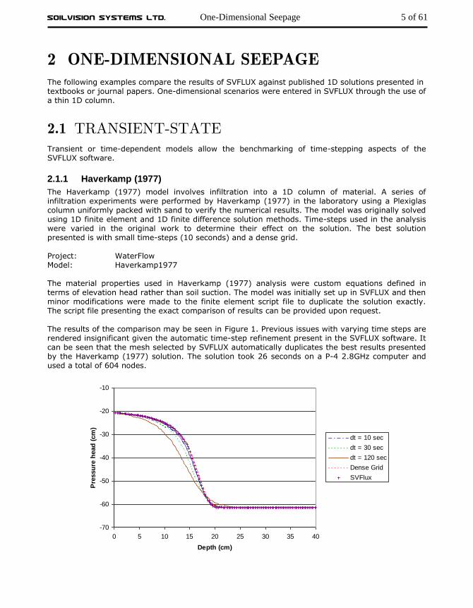
The Haverkamp (1977) model involves infiltration into a 1D column of material. A series of infiltration experiments were performed by Haverkamp (1977) in the laboratory using a Plexiglas column uniformly packed with sand to verify the numerical results. The model was originally solved using 1D finite element and 1D finite difference solution methods. Time-steps used in the analysis were varied in the original work to determine their effect on the solution. The best solution presented is with small time-steps (10 seconds) and a dense grid.
Project: WaterFlow Model: Haverkamp1977 The material properties used in Haverkamp (1977) analysis were custom equations defined in terms of elevation head rather than soil suction. The model was initially set up in SVFLUX and then minor modifications were made to the finite element script file to duplicate the solution exactly. The script file presenting the exact comparison of results can be provided upon request. The results of the comparison may be seen in Figure 1. Previous issues with varying time steps are rendered insignificant given the automatic time-step refinement present in the SVFLUX software. It can be seen that the mesh selected by SVFLUX automatically duplicates the best results presented by the Haverkamp (1977) solution. The solution took 26 seconds on a P-4 2.8GHz computer and used a total of 604 nodes.
-70
-60
-50
-40
-30
-20
-10
0 5 10 15 20 25 30 35 40
Depth (cm)
Pre
ssu
re h
ead
(cm
)
dt = 10 sec
dt = 30 sec
dt = 120 sec
Dense Grid
SVFlux
SoilVision Systems Ltd. One-Dimensional Seepage 6 of 61
Figure 1 Comparison between SVFLUX and Haverkamp (1977) as presented by Celia (1990)
2.1.2 Celia (1990)
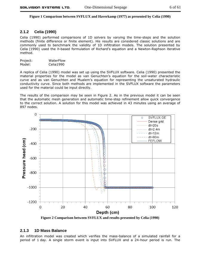
Celia (1990) performed comparisons of 1D solvers by varying the time-steps and the solution methods (finite difference or finite element). His results are considered classic solutions and are commonly used to benchmark the validity of 1D infiltration models. The solution presented by Celia (1990) used the h-based formulation of Richard’s equation and a Newton-Raphson iterative method. Project: WaterFlow Model: Celia1990 A replica of Celia (1990) model was set up using the SVFLUX software. Celia (1990) presented the material properties for the model as van Genuchten’s equation for the soil-water characteristic curve and as van Genuchten and Mualem’s equation for representing the unsaturated hydraulic
conductivity curve. Since both methods are implemented in the SVFLUX software the parameters used for the material could be input directly. The results of the comparison may be seen in Figure 2. As in the previous model it can be seen that the automatic mesh generation and automatic time-step refinement allow quick convergence to the correct solution. A solution for this model was achieved in 43 minutes using an average of 897 nodes.
Figure 2 Comparison between SVFLUX and results presented by Celia (1990)
2.1.3 1D Mass Balance
An infiltration model was created which verifies the mass-balance of a simulated rainfall for a period of 1 day. A single storm event is input into SVFLUX and a 24-hour period is run. The

SoilVision Systems Ltd. One-Dimensional Seepage 7 of 61
reported total flow into the 1D column should be equal to the amount of rainfall if calculations are correct. Zero flux boundaries on three sides of the model disallow any flux in or out of the model with the exception of the top boundary. Project: Columns Model: Day1
Precipitation: 0.1 m3/day/m2
Material: Grey Till ksat: 0.9 m/day
Figure 3 Soil-water characteristic curve for 1D mass-balance model
The results of the 1D model may be summarized as follows:
Application: 0.1 m3/day/m2 x 0.1 m2 = 0.01 m3/day Intensity: starts 9:00 am
ends 17:00 (5:00pm)
Reported flux in: 0.010043 m3/day Error: 0.43%
2.1.4 Clausnitzer (1991)
Lenhard et al. (1991) conducted an air-water flow experiment with a 72-cm vertical soil column to measure water content and pressure distributions over time that resulted from a fluctuating water table scenario. Clausnitzer (1991) used the 1D finite element method to simulate this column experiment. In this verification example, the finite element solution is simulated in 1D using SVFLUX, and the results are compared with the Clausnitzer’s results for the non-hysteretic condition. Project: WaterFlow Model: Clausnitzer1991 The column is filled with one homogeneous soil with saturated and unsaturated properties as shown in Table 2 and Figure 5. The initial condition is a Constant Head of 0.695 m. This means that
0
0.05
0.1
0.15
0.2
0.25
0.3
0.35
0.4
0.45
1e-3 1e-2 1e-1 1e+0 1e+1 1e+2 1e+3 1e+4 1e+5 1e+6
Soil suction (kPa)
Laboratory Interpolated Fredund and Xing Fit Laboratory Data
SoilVision Systems Ltd. One-Dimensional Seepage 8 of 61
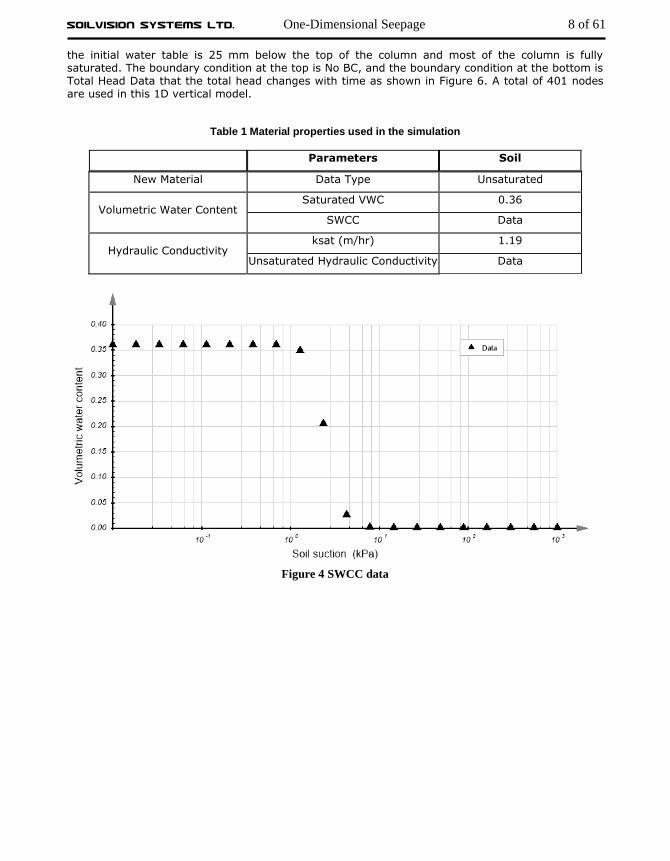
the initial water table is 25 mm below the top of the column and most of the column is fully saturated. The boundary condition at the top is No BC, and the boundary condition at the bottom is Total Head Data that the total head changes with time as shown in Figure 6. A total of 401 nodes are used in this 1D vertical model.
Table 1 Material properties used in the simulation
Parameters Soil
New Material Data Type Unsaturated
Volumetric Water Content Saturated VWC 0.36
SWCC Data
Hydraulic Conductivity ksat (m/hr) 1.19
Unsaturated Hydraulic Conductivity Data
Figure 4 SWCC data

SoilVision Systems Ltd. One-Dimensional Seepage 9 of 61
Figure 5 Unsaturated hydraulic conductivity data
Figure 6 Head Data boundary condition at the bottom of the column
Figure 7 shows the Volumetric Water Content (VWC) results from SVFLUX and Clausnitzer (1991) at five different locations, P1 (0.69 m), P2 (0.59 m), P3 (0.49 m), P4 (0.39 m) and P5 (0.29 m). The SVFLUX GE results have a good agreement with the results from Claunitzer (1991).

SoilVision Systems Ltd. One-Dimensional Seepage 10 of 61
Figure 7 vwc results at different locations for the non-hysteretic condition from SVFLUX and
Clausnitzer (1991)
2.1.5 Evaporation - Wilson (1990)
Project: USMEP Model: LimitingFunction1997_SVFlux, WilsonPenman1994_SVFlux, EmpiricalAE_SVFlux The classic solution to the coupling of material-atmosphere equations is presented by Wilson (1990). In Wilson’s PhD thesis (1990), a column of sand was subjected to drying in a laboratory environment in which the temperature and relative humidity were controlled. Measurements of
actual evaporation and the distributions of temperature along the column depth were obtained, providing several measures that can be used for the verification of the numerical model.
2.1.5.1 Model geometry and boundary conditions
A Modified Penman approach to the calculation of actual evaporation was presented in the thesis (hereafter termed the Wilson-Penman method). Wilson (1990) coded a 1D finite element package termed “Flux” in order to compare the physical results to a numerical solution. The geometry and configuration of the column may be seen in the following figure.

SoilVision Systems Ltd. One-Dimensional Seepage 11 of 61
Figure 8 Numerical simulation of the drying column test (Wilson, 1990)
An initial comparison to the results obtained by Wilson (1990) was performed by Gitirana (2004) using the FlexPDE solver used by SVFLUX. The FlexPDE formulation presented by Gitirana (2004) included full coupling of the temperature partial differential equations. The results of this work are presented in Figure 9.
Figure 9 Results of Gitirana (2004) as compared to Wilson (1990)
Three approaches are available to calculate the actual evaporation: Wilson-Penman AE (Wilson, 1994), Limiting-Function AE (Wilson et al., 1997), and Empirical AE (Wilson et al., 1997). Each approach can be simulated with the fully coupled water flow and heat using SVFLUX and SVHEAT. However, this benchmark only presents uncoupled evaporative simulations using SVFLUX package. Please see the SVHEAT Verification Manual for the results of the fully coupling simulations.
2.1.5.2 Material properties
The material properties in Wilson (1990) thesis are presented as follows. The ksat value used in the numerical modeling is presented as 310–5 m/s. The unsaturated hydraulic conductivity and
gravimetric water content values calculated using the Brooks and Corey estimation method are
presented in Table 6.2 (p. 252). In the “FLUX” code developed by Wilson (1990), the Brooks and Corey method of representing the SWCC and unsaturated hydraulic conductivity function. General hydraulic properties of the Beaver Creek sand are presented in Table 4.1 (p. 115).

SoilVision Systems Ltd. One-Dimensional Seepage 12 of 61
In this benchmark the soil water characteristic curve (SWCC) is approximated with Fredlund and Xing (1994) approach based on the Wilson (1990) measured data. The parameters for SWCC and hydraulic conductivity are presented in Table 2, Figure 10 and Figure 11.
Table 2 Material properties used in the simulation of Wilson’s evaporation benchmark
Material name Material properties Method and
parameters
Value unit
Beaver Creek Sand SWCC
Sat vwc 0.405 m3/m3
Fredlund and Xing
af 4.046 kPa
nf 1.692
mf 1.181
hr 12.415 kPa
Hydraulic
conductivity
Saturated k 2.592 m/day
Modified Campbell
Estimation
k min 10–7 m/day
Mcampbell p 15
Figure 10 Soil water characteristic curve of Beaver Creek Sand used in Wilson’s evaporation benchmark

SoilVision Systems Ltd. One-Dimensional Seepage 13 of 61
Figure 11 Hydraulic conductivity of unsaturated Beaver Creek Sand used in Wilson evaporation
benchmark
2.1.5.3 Results and discussion
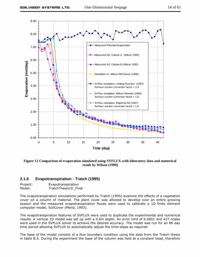
Exactly replicating this benchmark is technically challenging because the original code made use of an “L” parameter in the Brooks and Corey estimation in order to adjust the prediction. The use of such an “L” parameter is not currently implemented in SVFLUX. Therefore the Fredlund & Xing SWCC fitting curve and the Modified Campbell hydraulic conductivity fitting curve were used and adjusted to fit the data originally published by Wilson (1990) in Table 6.2. The experimental results obtained by Wilson (1990) were then again compared to SVFLUX. The results are shown in Figure 12. It can be seen from the results that a reasonable comparison is obtained. It was found the correction number is related to material properties such as the value of k min (see Table 2). It was also found in the course of the comparison that i) the separation point between the AE and PE as well as ii) the calculated AE later on in the calculation is highly sensitive to slight variations in the representation of the SWCC and the unsaturated hydraulic conductivity curve. To improve the modeling stability, an empirical correction number in SVFLUX is utilized to account for the steep suction gradient at the soil surface (see SVFLUX Theory Manual for details). The correction number in this benchmark was determined by trial and error.
SoilVision Systems Ltd. One-Dimensional Seepage 14 of 61
Figure 12 Comparison of evaporation simulated using SVFLUX with laboratory data and numerical
result by Wilson (1990)
2.1.6 Evapotranspiration - Tratch (1995)
Project: Evapotranspiration Model: TratchThesis1D_Final The evapotranspiration simulations performed by Tratch (1995) examine the effects of a vegetation cover on a column of material. The plant cover was allowed to develop over an entire growing season and the measured evapotranspiration fluxes were used to calibrate a 1D finite element computer model, SoilCover (Mend, 1993). The evapotranspiration features of SVFLUX were used to duplicate the experimental and numerical results. A vertical 1D model was set up with a 0.6m depth. An error limit of 0.0001 and 437 nodes were used in the SVFLUX solver to achieve the desired accuracy. The model was run for an 86 day time period allowing SVFLUX to automatically adjust the time-steps as required. The base of the model consists of a flow boundary condition using the data from the Tratch thesis in table B.5. During the experiment the base of the column was held at a constant head, therefore
0.00
1.00
2.00
3.00
4.00
5.00
6.00
7.00
8.00
9.00
0 5 10 15 20 25 30 35 40
Time (day)
Evap
ora
tio
n (
mm
/day)
Measured Potential Evaporation
Measured AE, Column A (Wilson 1992)
Measured AE, Column B (Wilson 1992)
Simulation of Wilson PhD thesis (1990)
SVFlux simulation, Limiting-Function (1997)
Surface suction correction factor = 1.8
SVFlux simulation, Wilson-Penman (1994)
Surface suction correction factor = 1.8
SVFlux simulation, Empirical AE (1997)
Surface suction correction factor = 1.8
SoilVision Systems Ltd. One-Dimensional Seepage 15 of 61
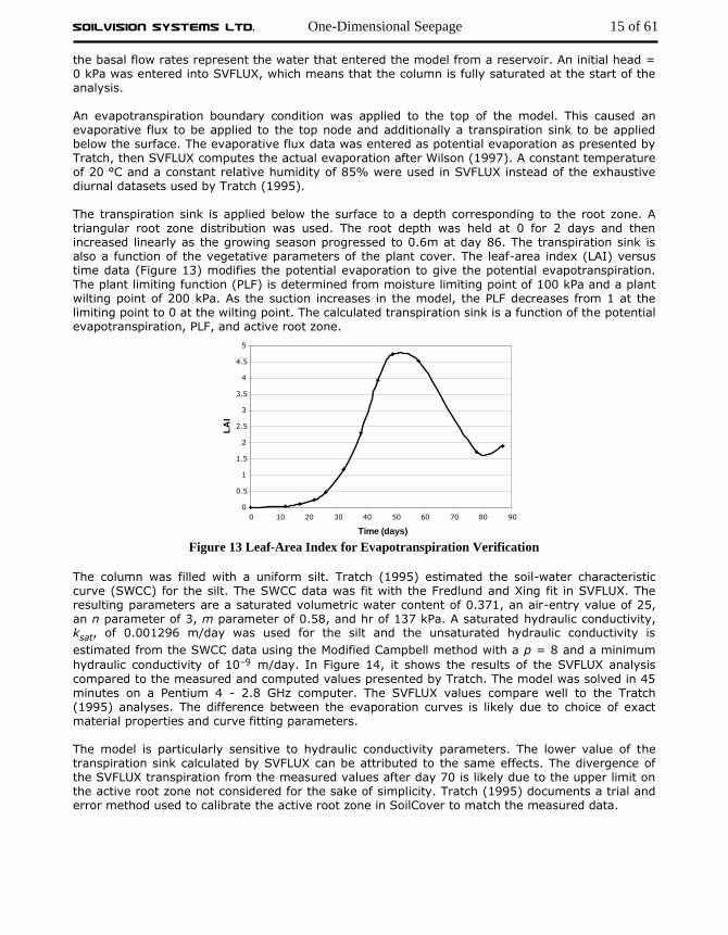
the basal flow rates represent the water that entered the model from a reservoir. An initial head = 0 kPa was entered into SVFLUX, which means that the column is fully saturated at the start of the analysis. An evapotranspiration boundary condition was applied to the top of the model. This caused an evaporative flux to be applied to the top node and additionally a transpiration sink to be applied below the surface. The evaporative flux data was entered as potential evaporation as presented by Tratch, then SVFLUX computes the actual evaporation after Wilson (1997). A constant temperature of 20 °C and a constant relative humidity of 85% were used in SVFLUX instead of the exhaustive diurnal datasets used by Tratch (1995). The transpiration sink is applied below the surface to a depth corresponding to the root zone. A triangular root zone distribution was used. The root depth was held at 0 for 2 days and then increased linearly as the growing season progressed to 0.6m at day 86. The transpiration sink is also a function of the vegetative parameters of the plant cover. The leaf-area index (LAI) versus time data (Figure 13) modifies the potential evaporation to give the potential evapotranspiration. The plant limiting function (PLF) is determined from moisture limiting point of 100 kPa and a plant wilting point of 200 kPa. As the suction increases in the model, the PLF decreases from 1 at the limiting point to 0 at the wilting point. The calculated transpiration sink is a function of the potential evapotranspiration, PLF, and active root zone.
Figure 13 Leaf-Area Index for Evapotranspiration Verification
The column was filled with a uniform silt. Tratch (1995) estimated the soil-water characteristic curve (SWCC) for the silt. The SWCC data was fit with the Fredlund and Xing fit in SVFLUX. The resulting parameters are a saturated volumetric water content of 0.371, an air-entry value of 25, an n parameter of 3, m parameter of 0.58, and hr of 137 kPa. A saturated hydraulic conductivity, ksat, of 0.001296 m/day was used for the silt and the unsaturated hydraulic conductivity is
estimated from the SWCC data using the Modified Campbell method with a p = 8 and a minimum
hydraulic conductivity of 10–9 m/day. In Figure 14, it shows the results of the SVFLUX analysis
compared to the measured and computed values presented by Tratch. The model was solved in 45 minutes on a Pentium 4 - 2.8 GHz computer. The SVFLUX values compare well to the Tratch (1995) analyses. The difference between the evaporation curves is likely due to choice of exact material properties and curve fitting parameters. The model is particularly sensitive to hydraulic conductivity parameters. The lower value of the transpiration sink calculated by SVFLUX can be attributed to the same effects. The divergence of the SVFLUX transpiration from the measured values after day 70 is likely due to the upper limit on the active root zone not considered for the sake of simplicity. Tratch (1995) documents a trial and error method used to calibrate the active root zone in SoilCover to match the measured data.
0
0.5
1
1.5
2
2.5
3
3.5
4
4.5
5
0 10 20 30 40 50 60 70 80 90
Time (days)
LA
I

SoilVision Systems Ltd. One-Dimensional Seepage 16 of 61
Figure 14 Comparisons between SVFLUX and results presented by Tratch (1995)
2.1.7 Gitirana (2005) Infiltration Examples
Project: Columns Models: InfiltrationWithRO_Gitirana2005_prec1ksat;
InfiltrationWithRO_Gitirana2005_prec1p5ksat; InfiltrationWithRO_Gitirana2005_prec2ksat; InfiltrationWithRO_Gitirana2005_prec4ksat; InfiltrationWithRO_Gitirana2005_prec10ksat
Gitirana (2005) presented a series of numerical models designed to test the ability of seepage software to handle cases of varying infiltration. The specific initiative involved determining the reasonableness of runoff calculations given increasing application of top boundary flux. For the series of models created each one had a varying application intensity scaled to the saturated hydraulic conductivity of the model. The models were all unsaturated and homogeneous models but each displayed the appropriate decay in actual infiltration, which would occur as the models became saturated and the amount of runoff therefore increased. Application rates of 1x, 1.5x, 2x, 4x, and 10x saturated hydraulic conductivity were set up. The benchmarks also demonstrate the robustness of the numerical model in handling cases of increasingly high precipitation events. As the intensity of the precipitation increases, it becomes
increasingly difficult to handle the increase numerically. SVFLUX admirably handles intensity applications up to 10x ksat. It is therefore recommended to evaluate soil cover models in light of how the intensities compare to the ksat of the top material in the numerical model. In the series of models created a constant flux is applied to the top of the model. The model eventually saturates and runoff begins to occur. This is demonstrated in the following figures which match well with the original results presented by Gitirana (2005).

SoilVision Systems Ltd. One-Dimensional Seepage 17 of 61
Figure 15 Graph of infiltration rate versus time
Figure 16 Graph of ratio of infiltration rate / precipitation rate versus time
It can be seen from the preceding figures that the SVFLUX software performs exceptionally well in solving under extreme conditions.
0
100
200
300
400
500
600
700
800
0 1 2 3 4 5 6 7
Infi
ltra
tio
n r
ate
, m
m/d
ay
Time, days
Precipitation rate, P = 10 ksat
P = 4 ksat
P = 2 ksat
P = 1.5 ksat
P = 1 ksat
0.0
0.2
0.4
0.6
0.8
1.0
1.2
0 1 2 3 4 5 6 7
Infi
ltra
tio
n r
ate
/ P
rec
ipit
ati
on
ra
te
Time, days
Precipitation rate, P = 1 ksat
P = 4 ksat
P = 2 ksat
P = 1.5 ksat
P = 10 ksat

SoilVision Systems Ltd. Two-Dimensional Seepage 18 of 61
3 TWO-DIMENSIONAL SEEPAGE Various models are used to verify the validity of the solutions provided by the SVFLUX software. Comparisons are made either to textbook solutions, journal-published solutions, or other software packages.
3.1 STEADY-STATE The first steady-state model used to compare the two software packages involves flow beneath a concrete gravity dam. The second model involves flow through an earth fill dam. Each scenario begins with a brief description of the model followed by a comparison of the results from Seep/W and SVFLUX.
3.1.1 2D Cutoff
Project: EarthDams Model: Cutoff
Figure 17 Mesh from SVFLUX solver (Pentland, 2000)
Figure 18 Mesh from Seep/W (Pentland, 2000)
SoilVision Systems Ltd. Two-Dimensional Seepage 19 of 61
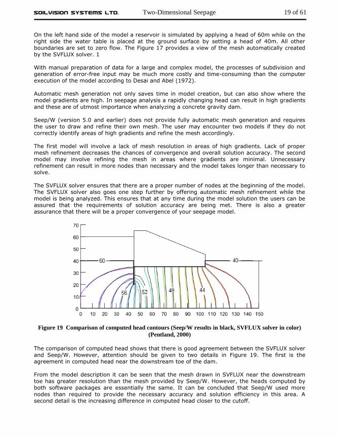
On the left hand side of the model a reservoir is simulated by applying a head of 60m while on the right side the water table is placed at the ground surface by setting a head of 40m. All other boundaries are set to zero flow. The Figure 17 provides a view of the mesh automatically created by the SVFLUX solver. 1 With manual preparation of data for a large and complex model, the processes of subdivision and generation of error-free input may be much more costly and time-consuming than the computer execution of the model according to Desai and Abel (1972). Automatic mesh generation not only saves time in model creation, but can also show where the model gradients are high. In seepage analysis a rapidly changing head can result in high gradients
and these are of utmost importance when analyzing a concrete gravity dam. Seep/W (version 5.0 and earlier) does not provide fully automatic mesh generation and requires the user to draw and refine their own mesh. The user may encounter two models if they do not correctly identify areas of high gradients and refine the mesh accordingly. The first model will involve a lack of mesh resolution in areas of high gradients. Lack of proper mesh refinement decreases the chances of convergence and overall solution accuracy. The second model may involve refining the mesh in areas where gradients are minimal. Unnecessary refinement can result in more nodes than necessary and the model takes longer than necessary to solve. The SVFLUX solver ensures that there are a proper number of nodes at the beginning of the model. The SVFLUX solver also goes one step further by offering automatic mesh refinement while the model is being analyzed. This ensures that at any time during the model solution the users can be assured that the requirements of solution accuracy are being met. There is also a greater assurance that there will be a proper convergence of your seepage model.
Figure 19 Comparison of computed head contours (Seep/W results in black, SVFLUX solver in color)
(Pentland, 2000)
The comparison of computed head shows that there is good agreement between the SVFLUX solver and Seep/W. However, attention should be given to two details in Figure 19. The first is the agreement in computed head near the downstream toe of the dam. From the model description it can be seen that the mesh drawn in SVFLUX near the downstream toe has greater resolution than the mesh provided by Seep/W. However, the heads computed by both software packages are essentially the same. It can be concluded that Seep/W used more nodes than required to provide the necessary accuracy and solution efficiency in this area. A second detail is the increasing difference in computed head closer to the cutoff.

SoilVision Systems Ltd. Two-Dimensional Seepage 20 of 61
From Figure 17 and Figure 18 in the model description it can be seen that the SVFLUX solver has provided a much denser mesh than Seep/W in this area. The accuracy of a finite element solution can be improved by one of two methods: either by refining the mesh, or by selecting higher order displacement models (Desai and Abel, 1972). It appears that the difference in the solved heads is the result of the denser mesh provided by the SVFLUX solver. While the differences are small in this model, the differences may become more apparent in a more complex model.
Figure 20 Computed vectors for SVFLUX solver (Pentland, 2000)
Figure 21 Computed vectors for Seep/W (Pentland, 2000)
The comparison of computed gradients shows general agreement between the two software packages. Hydraulic gradient, according to Darcy’s law is the change in head over a change in length, (Freeze and Cherry, 1979). It may be hard to detect in Figure 20 and Figure 21, but there appears to be differences in the computed gradients for the same reason as stated for the comparison of the computed heads.
SoilVision Systems Ltd. Two-Dimensional Seepage 21 of 61
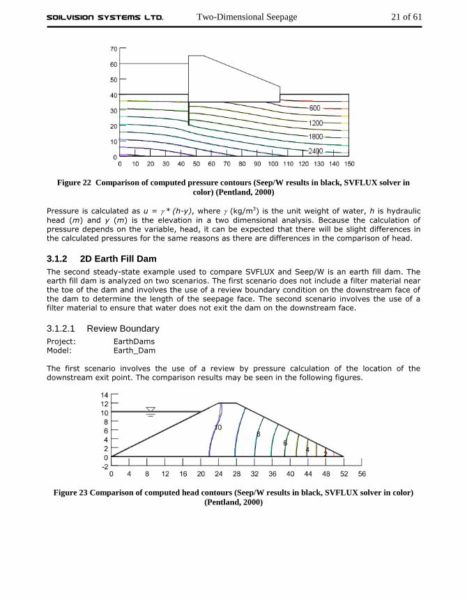
Figure 22 Comparison of computed pressure contours (Seep/W results in black, SVFLUX solver in
color) (Pentland, 2000)
Pressure is calculated as u = * (h-y), where (kg/m3) is the unit weight of water, h is hydraulic
head (m) and y (m) is the elevation in a two dimensional analysis. Because the calculation of pressure depends on the variable, head, it can be expected that there will be slight differences in the calculated pressures for the same reasons as there are differences in the comparison of head.
3.1.2 2D Earth Fill Dam
The second steady-state example used to compare SVFLUX and Seep/W is an earth fill dam. The earth fill dam is analyzed on two scenarios. The first scenario does not include a filter material near the toe of the dam and involves the use of a review boundary condition on the downstream face of the dam to determine the length of the seepage face. The second scenario involves the use of a filter material to ensure that water does not exit the dam on the downstream face.
3.1.2.1 Review Boundary
Project: EarthDams Model: Earth_Dam The first scenario involves the use of a review by pressure calculation of the location of the downstream exit point. The comparison results may be seen in the following figures.
Figure 23 Comparison of computed head contours (Seep/W results in black, SVFLUX solver in color)
(Pentland, 2000)
SoilVision Systems Ltd. Two-Dimensional Seepage 22 of 61
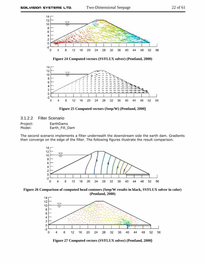
Figure 24 Computed vectors (SVFLUX solver) (Pentland, 2000)
Figure 25 Computed vectors (Seep/W) (Pentland, 2000)
3.1.2.2 Filter Scenario
Project: EarthDams
Model: Earth_Fill_Dam The second scenario implements a filter underneath the downstream side the earth dam. Gradients then converge on the edge of the filter. The following figures illustrate the result comparison.
Figure 26 Comparison of computed head contours (Seep/W results in black, SVFLUX solver in color)
(Pentland, 2000)
Figure 27 Computed vectors (SVFLUX solver) (Pentland, 2000)

SoilVision Systems Ltd. Two-Dimensional Seepage 23 of 61
Figure 28 Comparison of computed pressure contours (Seep/W results in black, SVFLUX solver in
color) (Pentland, 2000)
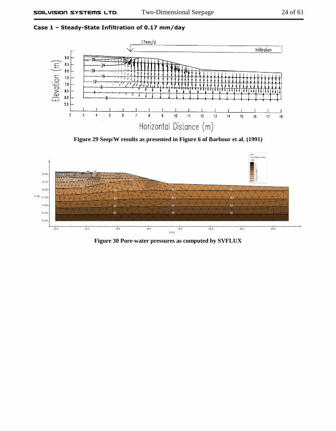
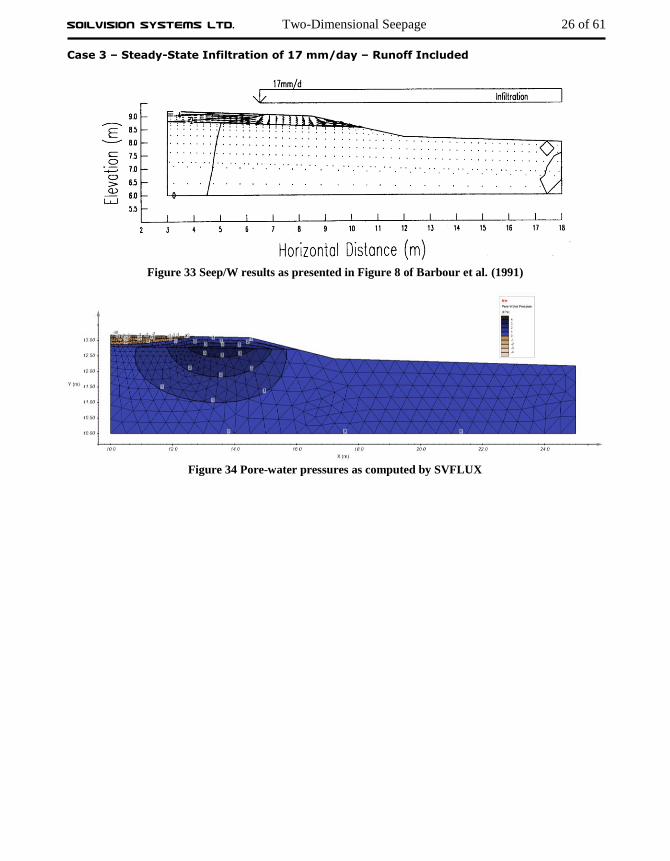
3.1.3 Roadways Subgrade Infiltration
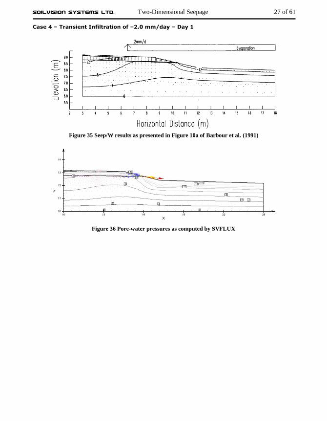
Project: Roadways Model: TRB01, TRB02, TRB03 The following scenarios are compared to Seep/W solutions previously published at the Canadian Geotechnical Conference in Toronto (Barbour et al., 1991). A typical cross-section of a roadway was created and various infiltration rates were applied to the shoulders of the highway. The resulting plots of pore-water pressure were presented. The results obtained when using SVFLUX show reasonable agreement to the previously calculated pore-water pressures. A slight difference between the computed water pressures beneath the highway can be attributed to the increased mesh density generated by SVFLUX. The results also indicate agreement between the calculation of runoff computed by SVFLUX and Seep/W.
SoilVision Systems Ltd. Two-Dimensional Seepage 24 of 61
Case 1 – Steady-State Infiltration of 0.17 mm/day
Figure 29 Seep/W results as presented in Figure 6 of Barbour et al. (1991)
Figure 30 Pore-water pressures as computed by SVFLUX
SoilVision Systems Ltd. Two-Dimensional Seepage 25 of 61
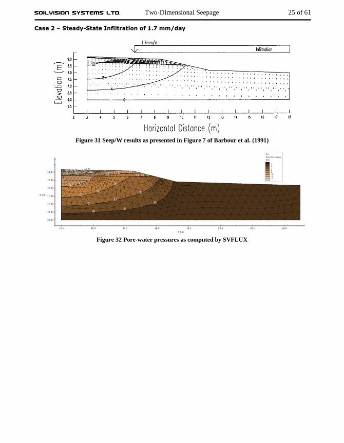
Case 2 – Steady-State Infiltration of 1.7 mm/day
Figure 31 Seep/W results as presented in Figure 7 of Barbour et al. (1991)
Figure 32 Pore-water pressures as computed by SVFLUX
SoilVision Systems Ltd. Two-Dimensional Seepage 26 of 61
Case 3 – Steady-State Infiltration of 17 mm/day – Runoff Included
Figure 33 Seep/W results as presented in Figure 8 of Barbour et al. (1991)
Figure 34 Pore-water pressures as computed by SVFLUX
SoilVision Systems Ltd. Two-Dimensional Seepage 27 of 61
Case 4 – Transient Infiltration of –2.0 mm/day – Day 1
Figure 35 Seep/W results as presented in Figure 10a of Barbour et al. (1991)
Figure 36 Pore-water pressures as computed by SVFLUX

SoilVision Systems Ltd. Two-Dimensional Seepage 28 of 61
Case 5 – Transient Infiltration of –2.0 mm/day – Day 10
Figure 37 Seep/W results as presented in Figure 10c of Barbour et al. (1991)
Figure 38 Pore-water pressures as computed by SVFLUX

SoilVision Systems Ltd. Two-Dimensional Seepage 29 of 61
3.1.4 Refraction Flow Example
Project: WaterFlow Model: Crespo This model provides verification of the “refraction law” when water passes from one material to another. The solution can be verified using either the flow lines or equipotentials since these lines are perpendicular in the steady-state solutions when k is isotropic. A square domain of 10m x 10m is set up. The outer perimeter is impervious with the exception of the specified head boundary conditions. The layer thicknesses are 4 m, 3 m, and 3 m. The model was documented by Crespo (1993).
Figure 39 Verification of the refraction law using SVFLUX
Result from the paper by Chapuis et al. (2001) is shown below.
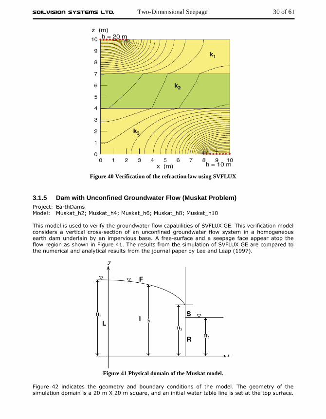
SoilVision Systems Ltd. Two-Dimensional Seepage 30 of 61
Figure 40 Verification of the refraction law using SVFLUX
3.1.5 Dam with Unconfined Groundwater Flow (Muskat Problem)
Project: EarthDams Model: Muskat_h2; Muskat_h4; Muskat_h6; Muskat_h8; Muskat_h10 This model is used to verify the groundwater flow capabilities of SVFLUX GE. This verification model considers a vertical cross-section of an unconfined groundwater flow system in a homogeneous earth dam underlain by an impervious base. A free-surface and a seepage face appear atop the flow region as shown in Figure 41. The results from the simulation of SVFLUX GE are compared to the numerical and analytical results from the journal paper by Lee and Leap (1997).
Figure 41 Physical domain of the Muskat model.
Figure 42 indicates the geometry and boundary conditions of the model. The geometry of the simulation domain is a 20 m X 20 m square, and an initial water table line is set at the top surface.

SoilVision Systems Ltd. Two-Dimensional Seepage 31 of 61
The boundary condition on the left side is assigned as Head Constant = 20 m. On the right side, the boundary condition from y = 0 m to y = H0 is assigned as Head Constant = H0, and from y = H0 to y = 20 m as Review Boundary Condition to determine the length of the seepage surface. Five different values of H0 (2 m, 4 m, 6 m, 8 m and 10 m) are tested.
Figure 42 The geometry and boundary conditions of the Muskat model
Table 2 shows the details of the material properties used in this example.
Table 3 Details of Muskat model material properties
Parameters Soil
Data Type Unsaturated
Saturated VWC 0.402
SWCC Fredlund and Xing Fit
ksat (m/s) 3.5e-4
Unsaturated Hydraulic Conductivity Modified Campbell Estimation
The results of the model and the comparisons with the results from Lee and Leap (1997) are summarized in Table 4. From the comparisons, it can be seen that the results from SVFLUX GE are close to those simulation results from Lee and Leap (1997). Some differences exist because the length of the seepage surface is very sensitive to the mesh density along that boundary and in the area close to it. The results can be viewed as comparable with the results in the paper.
Table 4 Results and comparisons
H1 (m) H0 (m) S (m)[1]
(Lee, 1997)
S (m)
(analytical)
S (m)
(SVFLUX GE)
Error[2]
20 2 5.7 5.3 5.54 2.8%
20 4 4.0 3.7 4.00 0.0%
20 6 2.7 2.4 2.80 3.6%
20 8 1.7 1.5 1.50 13.3%
20 10 0.9 0.8 1.00 10.0%
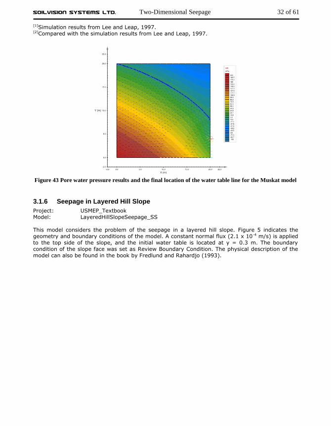
SoilVision Systems Ltd. Two-Dimensional Seepage 32 of 61
[1]Simulation results from Lee and Leap, 1997. [2]Compared with the simulation results from Lee and Leap, 1997.
Figure 43 Pore water pressure results and the final location of the water table line for the Muskat model
3.1.6 Seepage in Layered Hill Slope
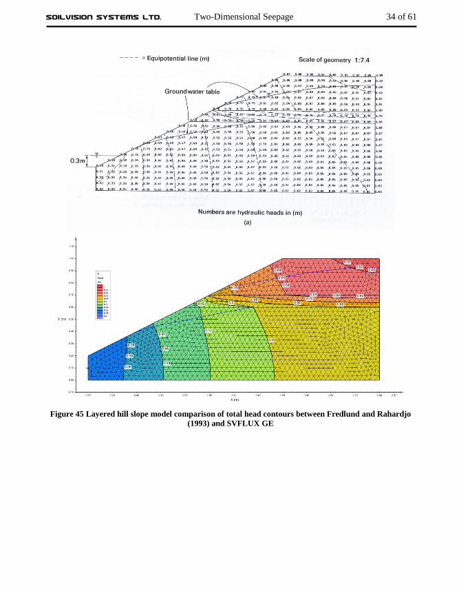
Project: USMEP_Textbook Model: LayeredHillSlopeSeepage_SS This model considers the problem of the seepage in a layered hill slope. Figure 5 indicates the geometry and boundary conditions of the model. A constant normal flux (2.1 x 10⁻⁴ m/s) is applied to the top side of the slope, and the initial water table is located at y = 0.3 m. The boundary condition of the slope face was set as Review Boundary Condition. The physical description of the model can also be found in the book by Fredlund and Rahardjo (1993).

SoilVision Systems Ltd. Two-Dimensional Seepage 33 of 61
Figure 44 Geometry and boundary conditions of the layered hill slope model
Two different unsaturated soils are used for the model. These consist of a medium sand and a fine sand with a lower hydraulic conductivity. The medium sand material is utilized for the bottom and top regions of the slope, and the fine sand material is used for the thin layer within the slope. Table
2 shows the detailed properties of the materials.
Table 5 Material properties used in the layered hill slope model
Parameters Medium sand Fine sand
Data Type Unsaturated Unsaturated
Saturated VWC 0.495 0.495
SWCC Fredlund and Xing Fit Fredlund and Xing Fit
ksat (m/s) 1.4e-3 5.5e-5
Unsaturated Hydraulic Conductivity Data Data
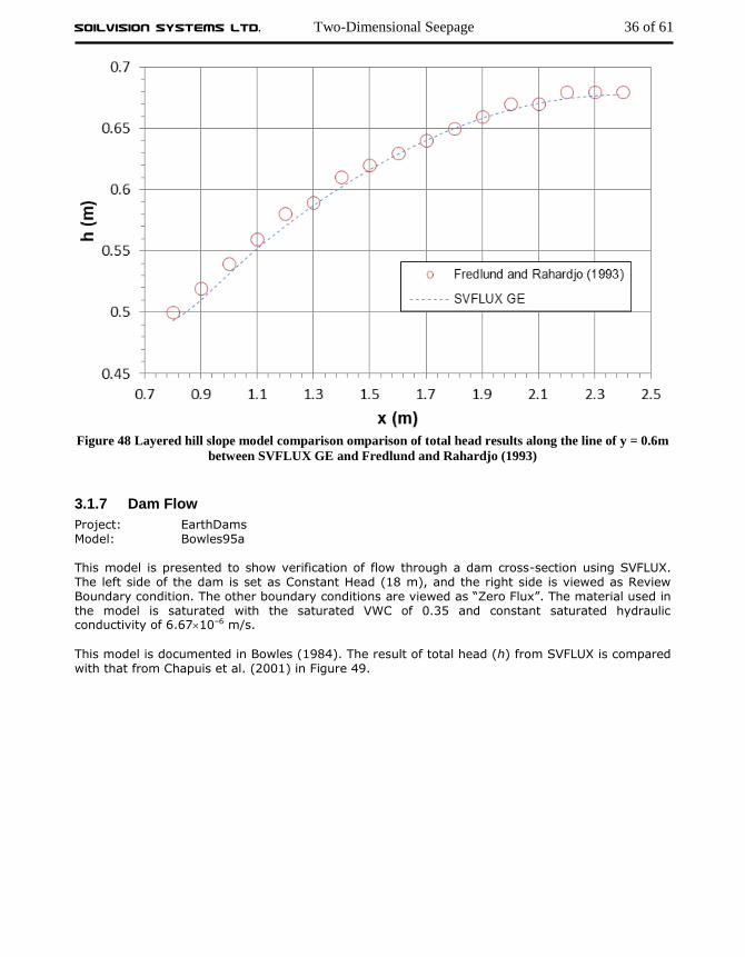
Figure 45 and Figure 46 show the total head (h) and pore water pressure (uw) results from SVFLUX GE. A physical comparison of the results of the SVFLUX GE contours to those obtained in the Fredlund and Rahardjo (1993) textbook shows close agreement. The results are quantitatively compared with those from Fredlund and Rahardjo (1993) along the lines of x = 1.6 m and y = 0.6 m as shown in Figure 47 and Figure 48, and comparisons further verify the correctness of the results from SVFLUX GE.
SoilVision Systems Ltd. Two-Dimensional Seepage 34 of 61
Figure 45 Layered hill slope model comparison of total head contours between Fredlund and Rahardjo
(1993) and SVFLUX GE

SoilVision Systems Ltd. Two-Dimensional Seepage 35 of 61
Figure 46 Layered hill slope model pore water pressure contour results from SVFLUX GE
Figure 47 Layered hill slope model comparison of total head results along the line of x = 1.6m between
SVFLUX GE and Fredlund and Rahardjo (1993)
SoilVision Systems Ltd. Two-Dimensional Seepage 36 of 61
Figure 48 Layered hill slope model comparison omparison of total head results along the line of y = 0.6m
between SVFLUX GE and Fredlund and Rahardjo (1993)
3.1.7 Dam Flow
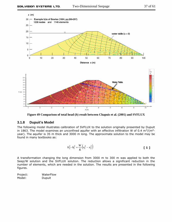
Project: EarthDams Model: Bowles95a This model is presented to show verification of flow through a dam cross-section using SVFLUX. The left side of the dam is set as Constant Head (18 m), and the right side is viewed as Review Boundary condition. The other boundary conditions are viewed as “Zero Flux”. The material used in the model is saturated with the saturated VWC of 0.35 and constant saturated hydraulic conductivity of 6.6710–6 m/s.
This model is documented in Bowles (1984). The result of total head (h) from SVFLUX is compared with that from Chapuis et al. (2001) in Figure 49.
SoilVision Systems Ltd. Two-Dimensional Seepage 37 of 61
Figure 49 Comparison of total head (h) result between Chapuis et al. (2001) and SVFLUX
3.1.8 Dupuit’s Model
The following model illustrates calibration of SVFLUX to the solution originally presented by Dupuit
in 1863. The model examines an unconfined aquifer with an effective infiltration W of 0.4 m3/(m2-
year). The aquifer is 35 m thick and 3000 m long. The approximate solution to the model may be found in many textbooks as:
22
21
21
22 xx
K
Whh [ 1 ]
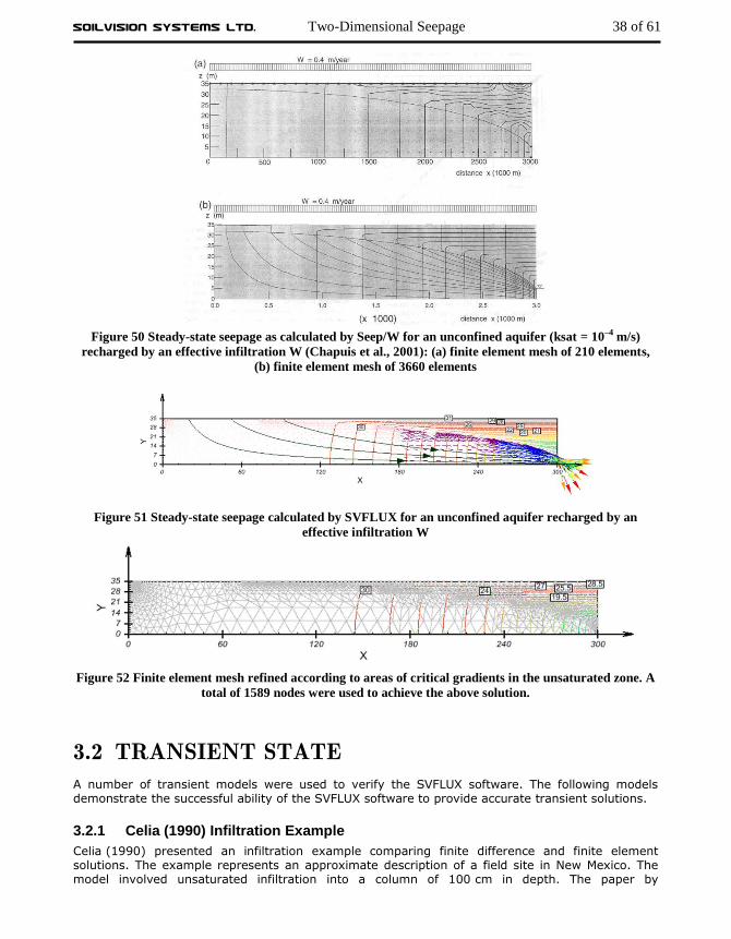
A transformation changing the long dimension from 3000 m to 300 m was applied to both the Seep/W solution and the SVFLUX solution. The reduction allows a significant reduction in the
number of elements, which are needed in the solution. The results are presented in the following figures. Project: WaterFlow Model: Dupuit
SoilVision Systems Ltd. Two-Dimensional Seepage 38 of 61
Figure 50 Steady-state seepage as calculated by Seep/W for an unconfined aquifer (ksat = 10–4 m/s)
recharged by an effective infiltration W (Chapuis et al., 2001): (a) finite element mesh of 210 elements,
(b) finite element mesh of 3660 elements
Figure 51 Steady-state seepage calculated by SVFLUX for an unconfined aquifer recharged by an
effective infiltration W
Figure 52 Finite element mesh refined according to areas of critical gradients in the unsaturated zone. A
total of 1589 nodes were used to achieve the above solution.
3.2 TRANSIENT STATE A number of transient models were used to verify the SVFLUX software. The following models demonstrate the successful ability of the SVFLUX software to provide accurate transient solutions.
3.2.1 Celia (1990) Infiltration Example
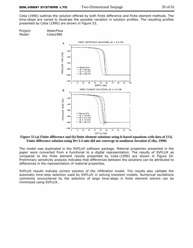
Celia (1990) presented an infiltration example comparing finite difference and finite element solutions. The example represents an approximate description of a field site in New Mexico. The model involved unsaturated infiltration into a column of 100 cm in depth. The paper by
SoilVision Systems Ltd. Two-Dimensional Seepage 39 of 61
Celia (1990) outlines the solution offered by both finite difference and finite element methods. The time-steps are varied to illustrate the possible variation in solution profiles. The resulting profiles presented by Celia (1990) are shown in Figure 53. Project: WaterFlow Model: Celia1990
Figure 53 (a) Finite difference and (b) finite element solutions using h-based equations with data of (13).
Finite difference solution using Dt=2.4 min did not converge in nonlinear iteration (Celia, 1990)
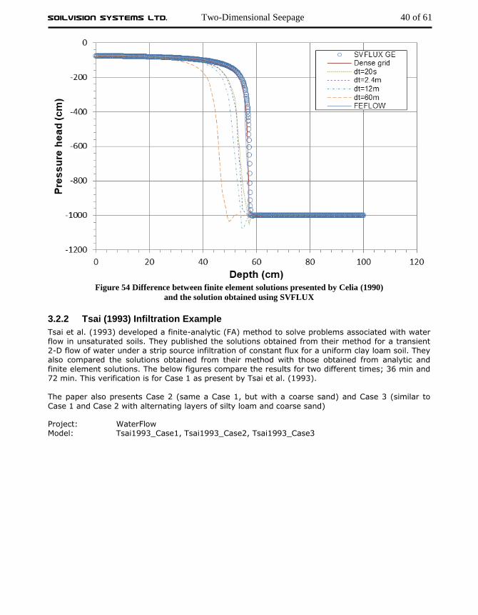
The model was duplicated in the SVFLUX software package. Material properties presented in the paper were converted from a functional to a digital representation. The results of SVFLUX as compared to the finite element results presented by Celia (1990) are shown in Figure 54. Preliminary sensitivity analysis indicates that differences between the solutions can be attributed to differences in the representation of material properties.
SVFLUX results indicate correct solution of the infiltration model. The results also validate the automatic time-step selection used by SVFLUX in solving transient models. Numerical oscillations commonly encountered by the selection of large time-steps in finite element solvers can be minimized using SVFLUX.
SoilVision Systems Ltd. Two-Dimensional Seepage 40 of 61
Figure 54 Difference between finite element solutions presented by Celia (1990)
and the solution obtained using SVFLUX
3.2.2 Tsai (1993) Infiltration Example
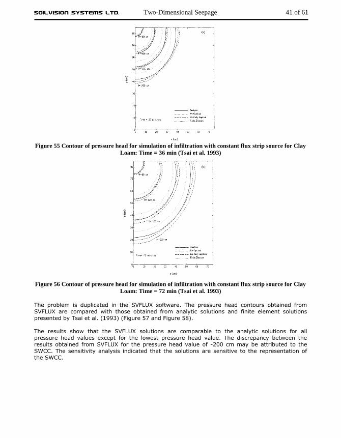
Tsai et al. (1993) developed a finite-analytic (FA) method to solve problems associated with water flow in unsaturated soils. They published the solutions obtained from their method for a transient 2-D flow of water under a strip source infiltration of constant flux for a uniform clay loam soil. They also compared the solutions obtained from their method with those obtained from analytic and finite element solutions. The below figures compare the results for two different times; 36 min and 72 min. This verification is for Case 1 as present by Tsai et al. (1993). The paper also presents Case 2 (same a Case 1, but with a coarse sand) and Case 3 (similar to
Case 1 and Case 2 with alternating layers of silty loam and coarse sand)
Project: WaterFlow Model: Tsai1993_Case1, Tsai1993_Case2, Tsai1993_Case3
SoilVision Systems Ltd. Two-Dimensional Seepage 41 of 61
Figure 55 Contour of pressure head for simulation of infiltration with constant flux strip source for Clay
Loam: Time = 36 min (Tsai et al. 1993)
Figure 56 Contour of pressure head for simulation of infiltration with constant flux strip source for Clay
Loam: Time = 72 min (Tsai et al. 1993)
The problem is duplicated in the SVFLUX software. The pressure head contours obtained from SVFLUX are compared with those obtained from analytic solutions and finite element solutions presented by Tsai et al. (1993) (Figure 57 and Figure 58). The results show that the SVFLUX solutions are comparable to the analytic solutions for all pressure head values except for the lowest pressure head value. The discrepancy between the results obtained from SVFLUX for the pressure head value of -200 cm may be attributed to the SWCC. The sensitivity analysis indicated that the solutions are sensitive to the representation of the SWCC.

SoilVision Systems Ltd. Two-Dimensional Seepage 42 of 61
Figure 57 Contour of pressure head for simulation of infiltration with constant flux strip source for Clay
Loam resulted from SVFLUX, Analytical, and Finite Element solutions: Time = 36 min
Figure 58 Contour of pressure head for simulation of infiltration with constant flux strip source for Clay
Loam resulted from SVFLUX, Analytical, and Finite Element solutions: Time = 72 min
3.2.3 Transient Phreatic Flow Subjected to Horizontal Seepage
Project: WaterFlow
Model: HorizontalPhreaticFlow This verification model considers transient seepage through a fully confined aquifer. The aquifer is 100 m long and 5 m thick. The aquifer has 10 m Constant Head on the left side and 5 m Constant Head on the right side, and the bottom and top sides are viewed as Zero Flux. The initial condition is viewed as a Constant Head of 5 m in the aquifer. Then seepage is examined in the x-direction with time. The geometry and boundary conditions of the model are shown in Figure 59.
0
10
20
30
40
50
60
70
80
0 10 20 30 40 50 60 70
x (cm)
y(c
m)
SVFlux
Analytical Solution from Paper
H = -200 cm
H = - 160 cm
H = - 120 cm
H = -80
Finite Element Solutions From
the Paper
0
10
20
30
40
50
60
70
80
0 10 20 30 40 50 60 70
x (cm)
y(c
m)
SVFlux
Analytical Solutions from PaperH = -200 cm
H = - 160 cm
H = - 120 cm
H = -80
Finite Element Solutions From
Paper

SoilVision Systems Ltd. Two-Dimensional Seepage 43 of 61
Figure 59 Geometry and boundary conditions of the horizonatal phreatic flow model
The material is assumed to be saturated with a hydraulic conductivity of 1 m/hr and the compressibility of the system due to a change in pore-water pressure (mv) of 0.1 1/kPa. Table 2
indicates the details of the material properties.
Table 6 Material properties used in the horizontal phreatic flow model
Tabs Parameters Soil
New Material Data Type Saturated
Volumetric Water Content Saturated VWC 0.4
Hydraulic Conductivity ksat (m/hr) 1.0
Compressibility of the system mv (1/kPa) 0.1
According to Tao and Xi (2006), in a semi-infinite aquifer bounded by a linear channel, during the period of that vertical seepage is equal to zero (or can be neglected) and that the channel-water stage is raised rapidly to an altitude, the transient phreatic flow-process is only affected by the horizontal seepage from the channel. Then, the J. G. Ferris Formula can be obtained,
, ,0
2w v
xh x t h x H erfc
kt
r m
h(x,t) – the total head at position x at time t,
h(x,0) – the total head at position x at the initial condition (5 m), ΔH – the head difference between the initial head distribution and the introduced head (5 m), erfc – the complimentary error function. Figure 60 shows the contour of total head at 600 hours. It can be seen that the values of head only change in the x-direction, so the vertical seepage can be neglected.
Figure 60 The contour of total head at 600 hours for the horizonatal phreatic flow model
A comparison of SVFLUX GE results and the analytical calculations at different time (100 hours,
200 hours, 400 hours and 600 hours) is shown in Figure 61. The agreement between SVFLUX GE and analytical results is good.

SoilVision Systems Ltd. Two-Dimensional Seepage 44 of 61
Figure 61 Comparison of SVFLUX GE and analytical results
SoilVision Systems Ltd. Axisymmetric Seepage 45 of 61
4 AXISYMMETRIC SEEPAGE Various models are used to verify the validity of the solutions provided by the SVFLUX software. Comparisons are made either to textbook solutions, journal-published solutions, or other software packages.
4.1 STEADY-STATE Axisymmetric Steady-State.
4.1.1 Pumping Well in an Aquifer
Project: WellPumping Model: AquiferConfined_Davis, AquiferUnconfined_Davis
This verification example simulates the radial flow from an aquifer towards a pumping well in a homogeneous and isotropic soil. This axisymmetric example concerns two kinds of aquifers, confined and unconfined, and both of the results from SVFLUX GE are compared with the analytical calculations according to Davis and Dewiest (1966). The comparisons show that SVFLUX GE matches the analytical results very well and verify the ability of SVFLUX GE in simulating the groundwater problem in the axisymmetric coordinates.
4.1.1.1 Confined Aquifer
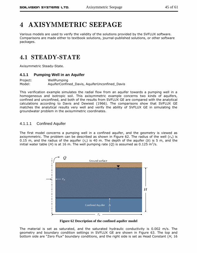
The first model concerns a pumping well in a confined aquifer, and the geometry is viewed as axisymmetric. The problem can be described as shown in Figure 62. The radius of the well (rw) is 0.15 m, and the radius of the aquifer (re) is 40 m. The depth of the aquifer (b) is 5 m, and the initial water table (H) is at 16 m. The well pumping rate (Q) is assumed as 0.125 m3/s.
Figure 62 Description of the confined aquifer model
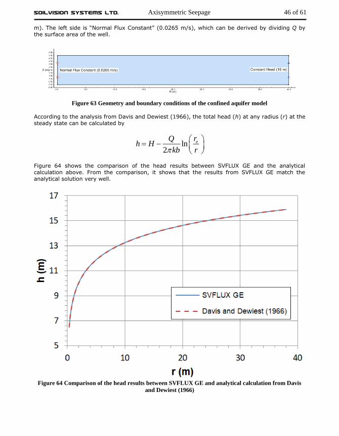
The material is set as saturated, and the saturated hydraulic conductivity is 0.002 m/s. The geometry and boundary condition settings in SVFLUX GE are shown in Figure 63. The top and bottom side are “Zero Flux” boundary conditions, and the right side is set as Head Constant (H, 16
SoilVision Systems Ltd. Axisymmetric Seepage 46 of 61
m). The left side is “Normal Flux Constant” (0.0265 m/s), which can be derived by dividing Q by the surface area of the well.
Figure 63 Geometry and boundary conditions of the confined aquifer model
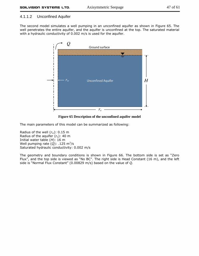
According to the analysis from Davis and Dewiest (1966), the total head (h) at any radius (r) at the steady state can be calculated by
ln2
erQh H
kb r
Figure 64 shows the comparison of the head results between SVFLUX GE and the analytical calculation above. From the comparison, it shows that the results from SVFLUX GE match the analytical solution very well.
Figure 64 Comparison of the head results between SVFLUX GE and analytical calculation from Davis
and Dewiest (1966)
SoilVision Systems Ltd. Axisymmetric Seepage 47 of 61
4.1.1.2 Unconfined Aquifer
The second model simulates a well pumping in an unconfined aquifer as shown in Figure 65. The well penetrates the entire aquifer, and the aquifer is unconfined at the top. The saturated material with a hydraulic conductivity of 0.002 m/s is used for the aquifer.
Figure 65 Description of the unconfined aquifer model
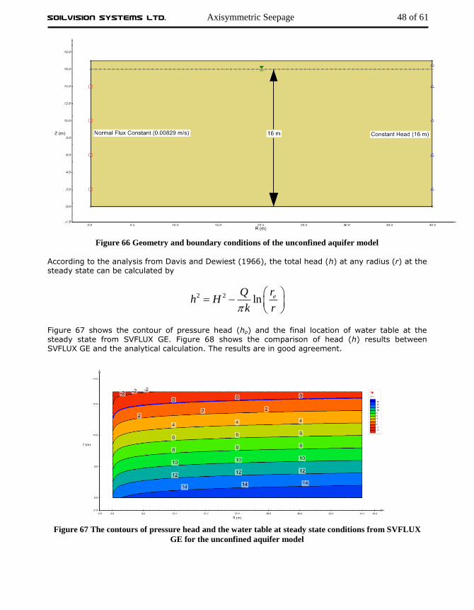
The main parameters of this model can be summarized as following: Radius of the well (rw): 0.15 m Radius of the aquifer (re): 40 m Initial water table (H): 16 m Well pumping rate (Q): .125 m3/s Saturated hydraulic conductivity: 0.002 m/s The geometry and boundary conditions is shown in Figure 66. The bottom side is set as “Zero Flux”, and the top side is viewed as “No BC”. The right side is Head Constant (16 m), and the left side is “Normal Flux Constant” (0.00829 m/s) based on the value of Q.
SoilVision Systems Ltd. Axisymmetric Seepage 48 of 61
Figure 66 Geometry and boundary conditions of the unconfined aquifer model
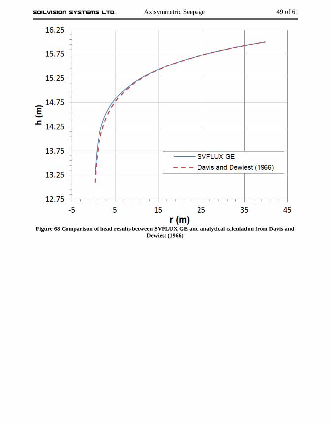
According to the analysis from Davis and Dewiest (1966), the total head (h) at any radius (r) at the steady state can be calculated by
2 2 ln erQh H
k r
Figure 67 shows the contour of pressure head (hp) and the final location of water table at the steady state from SVFLUX GE. Figure 68 shows the comparison of head (h) results between SVFLUX GE and the analytical calculation. The results are in good agreement.
Figure 67 The contours of pressure head and the water table at steady state conditions from SVFLUX
GE for the unconfined aquifer model
SoilVision Systems Ltd. Axisymmetric Seepage 49 of 61
Figure 68 Comparison of head results between SVFLUX GE and analytical calculation from Davis and
Dewiest (1966)

SoilVision Systems Ltd. Three-Dimensional Seepage 50 of 61
5 THREE-DIMENSIONAL SEEPAGE Three-dimensional seepage models are presented in this chapter to provide a forum to compare the results of the SVFLUX solver to the results of other seepage software and other documented examples. Both steady-state and transient models are considered.
5.1 STEADY-STATE The following models are presented as steady-state verification when time is assumed to be infinite.
5.1.1 3D Wedge
The following model illustrates the use of a wedge to perform calculations for a three-dimensional analysis. Flux sections are placed at various points in the model to compute water flow volumes. The hydraulic conductivity was set at 0.1 m/s. The error limit of the software had to be decreased to 0.00001 m/s in order to increase the solution accuracy. Project: WaterFlow Model: Wedge3D
Figure 69 Wedge3D model geometry
Flux 1: 144.844 m3/s Error: 0.00%
Flux 2: 144.838 m3/s Error: 0.00%
Flux 3: 144.762 m3/s Error: 0.06% Flux 4: 143.010 m3/s Error: 1.23%
Flux 1
Flux 2
Flux 3
Flux 4
508348
50
70
X
Y
Z

SoilVision Systems Ltd. Three-Dimensional Seepage 51 of 61
5.1.3 3D Well Object vs Cylinder
The purpose of the models in this section is to verify that the well object can successfully represent piezometric wells in a 3D scenario. A model with a cylinder representing a well is first created in order to prove the new Well object approach. The results of the cylinder are then compared to the new Well object approach. The new well object approach requires far fewer nodes in order to calculate resulting fluxes so there are significant benefits with the proposed new approach. The Well object uses a sink mechanism to simulate pumping in piezometric wells (see the SVFLUX Theory Manual for a further description). Project: WellPumping Model: Well_Object_3D and Slender_Cylinder_3D
Figure 70 Well_Object_3D model
Figure 71 Slender_Cylinder_3D model
In model Well_Object_3D (thereafter referred to as the “Well Model”), there is a Well object in the center of the model domain. The vertical screen length of the well is 20 m measured from the bottom of the well. The well object represents a well with zero radius. The well is enclosed by flux sections Flux1, Flux2, Flux3 and Flux4 as shown in Figure 70. So it is possible to investigate the total flow into the well when a pumping rate is applied. The model Slender_Cylinder_3D (thereafter referred to as the “Cylinder Model”) is the same as the model Well_Object_3D but makes use of a slender cylinder to replace the well object. The length L of the cylinder is 20 m and the radius R of the cylinder is 0.3 m.
SoilVision Systems Ltd. Three-Dimensional Seepage 52 of 61
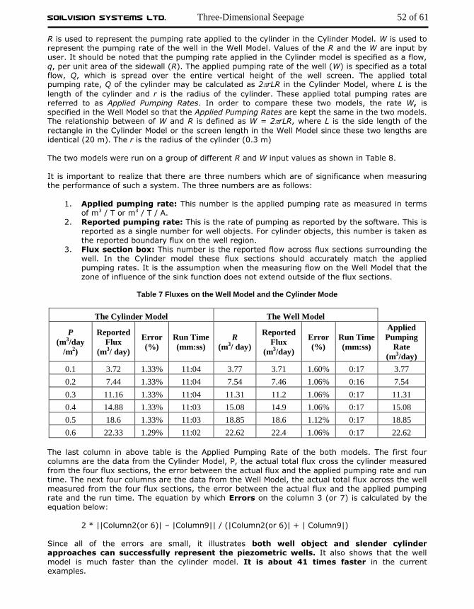
R is used to represent the pumping rate applied to the cylinder in the Cylinder Model. W is used to represent the pumping rate of the well in the Well Model. Values of the R and the W are input by user. It should be noted that the pumping rate applied in the Cylinder model is specified as a flow, q, per unit area of the sidewall (R). The applied pumping rate of the well (W) is specified as a total flow, Q, which is spread over the entire vertical height of the well screen. The applied total pumping rate, Q of the cylinder may be calculated as 2rLR in the Cylinder Model, where L is the
length of the cylinder and r is the radius of the cylinder. These applied total pumping rates are referred to as Applied Pumping Rates. In order to compare these two models, the rate W, is specified in the Well Model so that the Applied Pumping Rates are kept the same in the two models. The relationship between of W and R is defined as W = 2rLR, where L is the side length of the
rectangle in the Cylinder Model or the screen length in the Well Model since these two lengths are identical (20 m). The r is the radius of the cylinder (0.3 m) The two models were run on a group of different R and W input values as shown in Table 8. It is important to realize that there are three numbers which are of significance when measuring the performance of such a system. The three numbers are as follows:
1. Applied pumping rate: This number is the applied pumping rate as measured in terms of m3 / T or m3 / T / A.
2. Reported pumping rate: This is the rate of pumping as reported by the software. This is reported as a single number for well objects. For cylinder objects, this number is taken as the reported boundary flux on the well region.
3. Flux section box: This number is the reported flow across flux sections surrounding the well. In the Cylinder model these flux sections should accurately match the applied pumping rates. It is the assumption when the measuring flow on the Well Model that the zone of influence of the sink function does not extend outside of the flux sections.
Table 7 Fluxes on the Well Model and the Cylinder Mode
The Cylinder Model The Well Model
P
(m3/day
/m2)
Reported
Flux
(m3/ day)
Error
(%)
Run Time
(mm:ss)
R
(m3/ day)
Reported
Flux
(m3/day)
Error
(%)
Run Time
(mm:ss)
Applied
Pumping
Rate
(m3/day)
0.1 3.72 1.33% 11:04 3.77 3.71 1.60% 0:17 3.77
0.2 7.44 1.33% 11:04 7.54 7.46 1.06% 0:16 7.54
0.3 11.16 1.33% 11:04 11.31 11.2 1.06% 0:17 11.31
0.4 14.88 1.33% 11:03 15.08 14.9 1.06% 0:17 15.08
0.5 18.6 1.33% 11:03 18.85 18.6 1.12% 0:17 18.85
0.6 22.33 1.29% 11:02 22.62 22.4 1.06% 0:17 22.62
The last column in above table is the Applied Pumping Rate of the both models. The first four columns are the data from the Cylinder Model, P, the actual total flux cross the cylinder measured from the four flux sections, the error between the actual flux and the applied pumping rate and run time. The next four columns are the data from the Well Model, the actual total flux across the well measured from the four flux sections, the error between the actual flux and the applied pumping rate and the run time. The equation by which Errors on the column 3 (or 7) is calculated by the equation below:
2 * ||Column2(or 6)| – |Column9|| / (|Column2(or 6)| + | Column9|) Since all of the errors are small, it illustrates both well object and slender cylinder approaches can successfully represent the piezometric wells. It also shows that the well model is much faster than the cylinder model. It is about 41 times faster in the current examples.

SoilVision Systems Ltd. Three-Dimensional Seepage 53 of 61
The distributions of Pore Water Pressure (PWP) and Head (H) of both the Well Model and the Cylinder Model are the same for each row in above table. The Figure 72 and Figure 73 are the contour graphs of the Pore Water Pressure and Head of the Well Model and the Cylinder Model respectively for the case of the sixth row of the table, for example, the P is specified as –0.6 (m3/day/m2) in the cylinder model and the Rate is specified as –22.62 (m3/day) in the Well Model.
a) Pore Water Pressure b) Head
Figure 72 Contours of Pore Water Pressure and Head in the well model when R = -22.62 (m3 / day)
a) Pore Water Pressure b) Head
Figure 73 Contours of Pore Water Pressure and Head in the cylinder model when R = 0.62 (m3 / day /
m2)
5.1.4 Confined Aquifer 3D Ideal
Project: WellPumping Model: ConfinedAquifer3DIdeal These models are designed to verify the review by pressure boundary conditions as applied to a 3D well object within SVFLUX.
5.1.4.1 Purpose
A three dimensional SVFLUX model of an ideal confined aquifer was constructed to verify the implementation of wells against the classical Theis system. The Theis system is one-dimensional, of infinite extent, and includes the well as a boundary condition. The SVFLUX 3D model contained a well at the center, and a large domain to minimize the effect of the boundary on the drawdown near the well.
SoilVision Systems Ltd. Three-Dimensional Seepage 54 of 61
SVFLUX models wells as a sink term in the differential equations. This eliminates the singularity in the Theis model boundary condition, but spreads the local effect of the well over an area that may be larger than the physical well. The extent of the spread is user adjustable.
5.1.4.2 Theis System
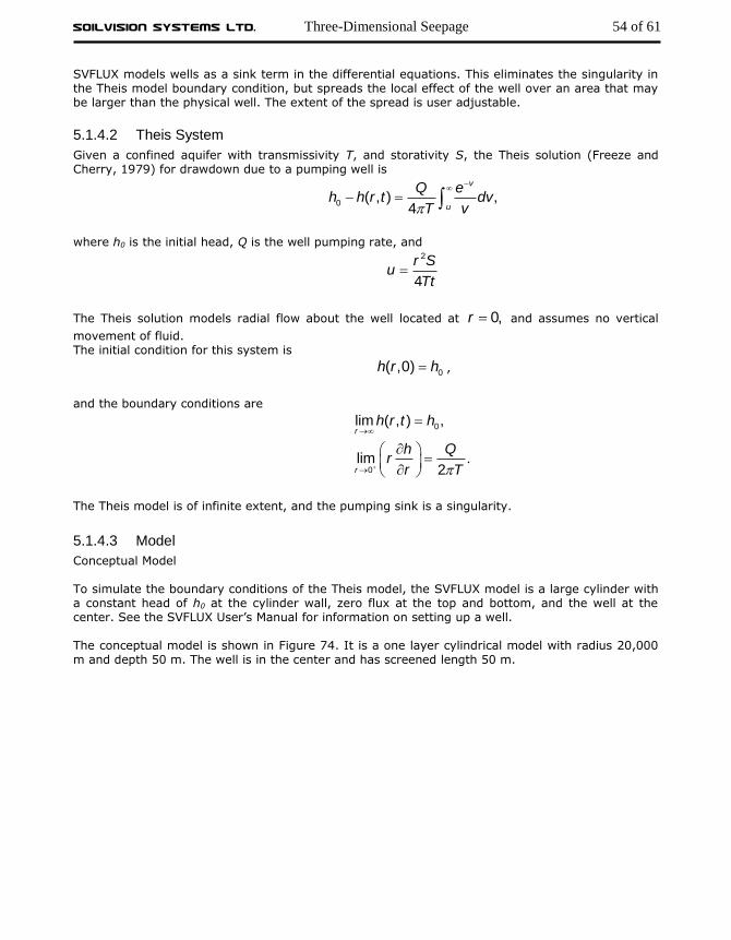
Given a confined aquifer with transmissivity T, and storativity S, the Theis solution (Freeze and Cherry, 1979) for drawdown due to a pumping well is
0( , ) ,
4
v
uh h r
et
Qdv
T v
where h0 is the initial head, Q is the well pumping rate, and
2
4u
r S
Tt
The Theis solution models radial flow about the well located at 0,r and assumes no vertical
movement of fluid. The initial condition for this system is
0( ,0)h r h ,
and the boundary conditions are
0
0
lim ( , ) ,
lim .2
r
r
h r t
Qr
h
h
r T
The Theis model is of infinite extent, and the pumping sink is a singularity.
5.1.4.3 Model
Conceptual Model To simulate the boundary conditions of the Theis model, the SVFLUX model is a large cylinder with a constant head of h0 at the cylinder wall, zero flux at the top and bottom, and the well at the center. See the SVFLUX User’s Manual for information on setting up a well. The conceptual model is shown in Figure 74. It is a one layer cylindrical model with radius 20,000 m and depth 50 m. The well is in the center and has screened length 50 m.

SoilVision Systems Ltd. Three-Dimensional Seepage 55 of 61
Figure 74 Conceptual Model for Theis Solution.
Numerical Model The SVFLUX model consists of two regions: ModelExtents and InnerRegion. InnerRegion was included to improve the resolution of the finite element mesh near the well. The SVFLUX model has the following properties:
General
System 3D
Type Transient
Units Metric
Time Units Day
World Coordinate System
X: Minimum -20,000 m
X: Maximum 20,000 m
Y: Minimum -20,000 m
Y: Maximum 20,000 m
Z: Minimum 0 m
Z: Maximum 50 m
Time (day)
Start Time 0
Initial Increment 10–5 (approx. 1 s)
Maximum Increment 1
End Time 10
5.1.4.4 Geometry and Properties
The well parameters are:
Line Mesh Spacing 2 m
Mesh Growth Coefficient 1
SoilVision Systems Ltd. Three-Dimensional Seepage 56 of 61
Influence Distance 2 m
Rate –8640 m3/day
The model geometry is:
Surfaces
Bottom 0 m
Top 50 m
Region: ModelExtents
Circle center (0 m, 0 m)
Circle radius 20,000 m
Region: InnerRegion
Circle center (0 m, 0 m)
Circle radius 100 m
The finite element solver and mesh parameters are all left at their defaults.
5.1.4.5 Material Properties
Material Properties (Aquifer—Sand):
Hydraulic Conductivity 8.64 m/day (10-4 m/s)
Transmissivity 432 m2/day (510-3 m2/s)
Porosity 0.4
Compressibility1 10-7 kPa-1
Storativity 4.910-5 1Aquifer compressibility. Water is treated as incompressible for this model.
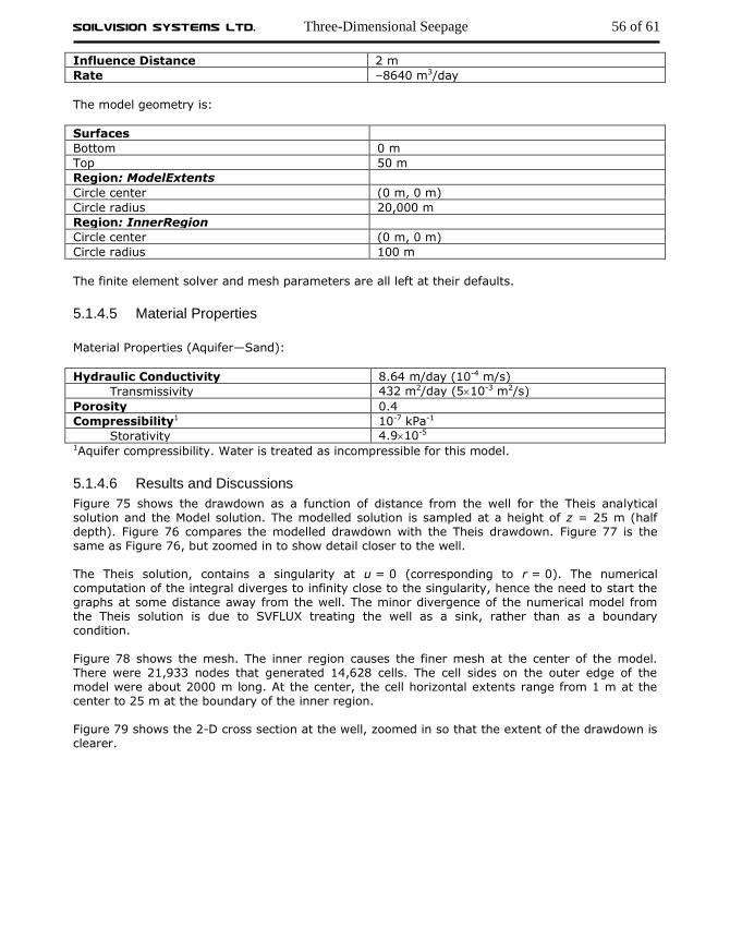
5.1.4.6 Results and Discussions
Figure 75 shows the drawdown as a function of distance from the well for the Theis analytical solution and the Model solution. The modelled solution is sampled at a height of z = 25 m (half depth). Figure 76 compares the modelled drawdown with the Theis drawdown. Figure 77 is the same as Figure 76, but zoomed in to show detail closer to the well. The Theis solution, contains a singularity at u = 0 (corresponding to r = 0). The numerical computation of the integral diverges to infinity close to the singularity, hence the need to start the graphs at some distance away from the well. The minor divergence of the numerical model from the Theis solution is due to SVFLUX treating the well as a sink, rather than as a boundary condition. Figure 78 shows the mesh. The inner region causes the finer mesh at the center of the model. There were 21,933 nodes that generated 14,628 cells. The cell sides on the outer edge of the model were about 2000 m long. At the center, the cell horizontal extents range from 1 m at the center to 25 m at the boundary of the inner region. Figure 79 shows the 2-D cross section at the well, zoomed in so that the extent of the drawdown is clearer.
SoilVision Systems Ltd. Three-Dimensional Seepage 57 of 61
Figure 75 Drawdown after 10 days. RMSD = 0.5 m.
Figure 76 Comparison of Theis and Model drawdown.
0
5
10
15
20
25
30
0 200 400 600 800 1000
Dra
wd
ow
n (
m)
r (m)
Theis
Model
y = 1.0025x - 0.052 R² = 1
0
5
10
15
20
25
30
0 5 10 15 20 25 30
Mo
del D
raw
do
wn
(m
)
Theis Drawdown (m)

SoilVision Systems Ltd. Three-Dimensional Seepage 58 of 61
Figure 77 Drawdown after 10 days out to 100 m.
Figure 78 Mesh distribution.
Figure 79 Drawdown after 10 days (vertical scale is zoomed 50 times).
0
5
10
15
20
25
30
0 20 40 60 80 100
Dra
wd
ow
n (
m)
r (m)
Theis
Model
SoilVision Systems Ltd. Three-Dimensional Seepage 59 of 61
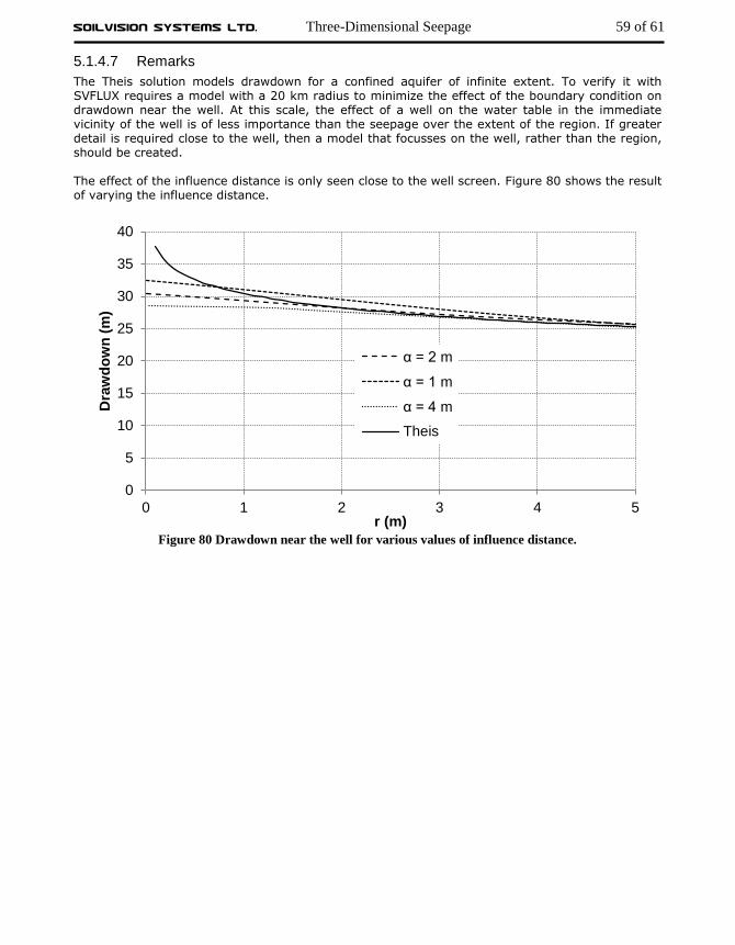
5.1.4.7 Remarks
The Theis solution models drawdown for a confined aquifer of infinite extent. To verify it with SVFLUX requires a model with a 20 km radius to minimize the effect of the boundary condition on drawdown near the well. At this scale, the effect of a well on the water table in the immediate vicinity of the well is of less importance than the seepage over the extent of the region. If greater detail is required close to the well, then a model that focusses on the well, rather than the region, should be created. The effect of the influence distance is only seen close to the well screen. Figure 80 shows the result of varying the influence distance.
Figure 80 Drawdown near the well for various values of influence distance.
0
5
10
15
20
25
30
35
40
0 1 2 3 4 5
Dra
wd
ow
n (
m)
r (m)
α = 2 m
α = 1 m
α = 4 m
Theis
SoilVision Systems Ltd. References 60 of 61
6 REFERENCES Barbour, S.L., Fredlund, D.G., Gan, J. K-M., and G.W. Wilson, (1991). Prediction of Moisture
Movement in Highway Subgrade Soils, 45th Canadian Geotechnical Conference, Toronto,
ON., Canada
Bowles, J.E., (1984). Physical and geotechnical properties of soils. 2nd ed. McGraw-Hill, New York.
Celia, M.A. and E.T. Bouloutas, (1990). A General Mass-Conservative Numerical Solution for the
Unsaturated Flow Equation. Water Resources Research, Vol. 26, No. 7, pp. 1483-1496, July.
Chapuis, Robert P., Chenaf, D., Bussiere, B., Aubertin, M., R. Crespo, (2001). A user’s approach to
assess numerical codes for saturated and unsaturated seepage conditions. Canadian Geotechnical Journal, 38: 1113-1126.
Clausnitzer, V.: Beitrag zur Bildung und Verifikation von Parametermodellen der
Mehrphasenstr¨omung in por¨osen Medien (contribution to the development and verification of parametric models for multiphase flow in porous media). Master’s thesis, Techn. University of Dresden, Dresden, Germany (1991).
Crespo, R., (1993). Modelisation par elements finis des ecoulements a travers les ouvrages de
retenue et de confinement des residus miniers. M.Sc.A. thesis, Ecole Polytechnique de Montreal, Montreal.
Davis, S. N., & Dewiest, R. J. M. (1966). Hydrogeology John Wiley and Sons. New York, 463. Diersch, H. J. G. (2013). FEFLOW: finite element modeling of flow, mass and heat transport in
porous and fractured media. Springer Science & Business Media. Dupuit, J., (1863). Etudes theoriques et pratiques sur le mouvement des eaux dans les canaux
decouverts et a travers les terrains permeables. 2nd ed. Dunod, Paris. Gitirana, G., (2004). Weather-Related Geo-Hazard Assessment Model for Railway Embankment
Stability, PhD Thesis, University of Saskatchewan, Saskatoon, SK, Canada. Gitirana, G.G., Fredlund, M.D., Fredlund, D.G., (2005). Infilitration-Runoff Boundary Conditions in
Seepage Analysis, Canadian Geotechnical Conference, September 19-21, Saskatoon, Canada
Fredlund, D. G., & Rahardjo, H. (1993). Soil mechanics for unsaturated soils. John Wiley & Sons. Freeze, R. and Cherry, J. 1979. Groundwater. Prentice-Hall, pp314 – 319. Haverkamp, R., Vauclin, M., Touma, J., Wierenga, P.J., and G.Vachaud, (1977). A Comparison of
Numerical Simulation Models for One-Dimensional Infiltration, Soil Science Society of
America Journal, Vol. 41, No. 2. Lee, K. K., & Leap, D. I. (1997). Simulation of a free-surface and seepage face using boundary-
fitted coordinate system method. Journal of Hydrology, 196(1-4), 297-309. Lenhard, R. J., Parker, J. C., & Kaluarachchi, J. J. (1991). Comparing Simulated and Experimental
Hysteretic Two‐Phase Transient Fluid Flow Phenomena. Water Resources Research, 27(8),
2113-2124.

SoilVision Systems Ltd. References 61 of 61
MEND 1993. SoilCover user’s manual for evaporative flux model. University of Saskatchewan,
Saskatoon, SK, Canada. Pentland, J.S., (2000). Use of a General Partial Differential Equation Solver for Solution of Heat and
Mass Transfer Problems in Soils, University of Saskatchewan, Saskatoon, SK, Canada. FlexPDE 6 (2007). Reference Manual, PDE Solutions Inc., Spokane Valley, WA 99206. FlexPDE 7 (2017). Reference Manual, PDE Solutions Inc., Spokane Valley, WA 99206. Freeze, R. A. and J. Cherry, (1979). Groundwater. Prentice–Hall, Inc., Englewood Cliffs, New Jersey Tao, Y. Z., & Xi, D. Y. (2006). Rule of transient phreatic flow subjected to vertical and horizontal
seepage. Applied Mathematics and Mechanics, 27, 59-65.
Todd, D.K. (1980). Groundwater hydrology, 2nd ed. John Wiley & Sons, New York.
Tratch, D.J., (1995). A Geotechnical Engineering Approach to Plant Transpiration and Root Water
Uptake, University of Saskatchewan, Saskatoon, SK, Canada. Tratch, D.J., Wilson, G.W., and D.G. Fredlund, (1995). An introduction to analytical modeling of
plant transpiration for geotechnical engineers, Proceedings, 48th Canadian Geotechnical
Conference, Vancouver, BC, Canada, Vol. 2, pp. 771-780. Tsai, W. F., Chen, C. J., & Tien, H. C. (1993). Finite analytic numerical solutions for unsaturated
flow with irregular boundaries. Journal of Hydraulic Engineering, 119(11), 1274-1298. Wilson, W., (1990). Soil Evaporative Fluxes for Geotechnical Engineering Problems. PhD Thesis,
Department of Civil Engineering, University of Saskatchewan, Saskatoon, SK, Canada.