Vertex-centred Discretization of Multiphase Compositional

Computational Geosciences manuscript No.(will be inserted by the editor)

Vertex-centred Discretization of Multiphase CompositionalDarcy flows on General Meshes

R. Eymard · C. Guichard · R. Herbin · R. Masson

Received: date / Accepted: date

Abstract This paper concerns the discretization on

general 3D meshes of multiphase compositional Darcy

flows in heterogeneous anisotropic porous media. Ex-

tending Coats’ formulation [14] to an arbitrary number

of phases, the model accounts for the coupling of the

mass balance of each component with the pore volume

conservation and the thermodynamical equilibrium, and

dynamically manages phase appearance and disappear-

ance. The spatial discretization of the multiphase com-

positional Darcy flows is based on a generalization of

the Vertex Approximate Gradient scheme (VAG), al-

ready introduced for single phase diffusive problems in

[18]. It leads to an unconditionally coercive scheme for

arbitrary meshes and permeability tensors. The sten-

cil of this vertex-centred scheme typically comprises 27

points on topologically Cartesian meshes, and the num-ber of unknowns on tetrahedral meshes is considerably

reduced, compared with usual cell-centred approaches.

The efficiency of our approach is exhibited on the near-

well injection of miscible CO2 in a saline aquifer taking

into account the vaporization of H2O in the gas phase

as well as the precipitation of salt.

R. EymardUniversity of Paris-Est, France,E-mail: [email protected]

C. GuichardUniversity of Paris-Est, France,E-mail: [email protected]

R. HerbinUniversity of Aix-Marseille, France,E-mail: [email protected]

R. MassonUniversity of Nice Sophia Antipolis, France,E-mail: [email protected]

1 Introduction

Many applications require the simulation of composi-

tional multiphase Darcy flow in heterogeneous porous

media. In oil reservoir modelling, the compositional tri-

phase Darcy flow simulator is a key tool to predict and

optimize the production of a reservoir. In sedimentary

basin modelling, such models are used to simulate the

migration of the oil and gas phases in a basin satu-

rated with water at geological space and time scales.

The objectives are to predict the location of the po-

tential reservoirs as well as the quality and quantity

of oil trapped therein. In CO2 geological storage, com-

positional multiphase Darcy flow models are used to

optimize the injection of CO2 and to assess the long

term integrity of the storage. Finally, two-phase com-

positional Darcy flow models are used to study the gas

migration in nuclear waste repositories (which consist

of porous media saturated with water), and to assess

the safety of the storage.

The numerical simulation of such models first re-

lies on a proper formulation which can account for the

coupling of the mass and pore volume conservations

together with the thermodynamical equilibrium. A ma-

jor difficulty there is the management of phase appear-

ance and disappearance induced by the change of phase

reactions assumed to be at equilibrium. Many formula-

tions have been proposed mainly in the oil industry (see

[12] and the numerous references therein), and more

recently for the modelling of gas migration in nuclear

waste disposal (see for example [4], [9], [11]).

In the following, we propose an extension to an ar-

bitrary number of phases of Coats formulation [14] de-

signed for reservoir simulation. This formulation, which

is expressed in the natural variables of the thermody-

2 R. Eymard et al.

namical and hydrodynamical laws, has the main ad-

vantage of dealing with a large range of models. The

first resulting difficulty is the complex management of

a variable number of equations and unknowns at each

point of the computational domain.

The second difficulty is to exhibit a space-time dis-

cretization, coping with the strong coupling of both an

elliptic (or a parabolic) unknown, the pressure, and hy-

perbolic (or degenerate parabolic) unknowns, the vol-

ume and mole fractions. The standard industrial answer

is based on cell-centred finite volume schemes, which

can be efficiently combined with an Euler implicit time

integration to allow for large time steps and accurately

capture the change of phases fronts.

The main drawback of cell-centred finite volume

schemes is the difficulty to use them in the case of com-

plex meshes and heterogeneous anisotropic permeabili-

ties, which are unfortunately frequently encountered in

practice to represent the basin and reservoir geometries

and petrophysical properties.

Many progresses have been done during the last

decade, leading to the design of cell-centred schemes

which remain consistent in such situations. Among these,

let us mention for example the well-known O scheme in-

troduced in [1], [2], [15], [16], the L scheme [3], or the

Sushi scheme [17]. We also refer to [6], [7], and [8] for the

convergence analysis of cell-centred schemes in a general

framework. Nevertheless it is still a challenge to design a

cell-centred discretization of diffusive fluxes in the case

of general meshes and heterogeneous anisotropic diffu-

sion tensors, which is linear, unconditionally coercive

and “compact”, in the sense that the expression of the

discrete flux at a given face of the mesh may at most

involve the cells sharing a vertex with this face. For

example the O and L schemes are compact but their

coercivity is mesh and permeability tensor dependent.

On the other hand, the Sushi scheme is unconditionally

coercive but its stencil is not compact, since it involves

the neighbours of the neighbours of a given control vol-

ume.

Recently, a new discretization of diffusive equations,

the Vertex Approximate Gradient (VAG) scheme, using

both cell and vertex unknowns, has been introduced

in [18]. The cell unknowns can be eliminated locally

without any fill-in, leading to a compact vertex-centred

scheme, with a typical 27 points stencil for 3D topo-

logically Cartesian meshes. The VAG scheme is con-

sistent, unconditionally coercive, compact, and easy to

implement on general meshes and for heterogeneous

anisotropic diffusion tensors. In addition, it is exact on

cellwise affine solutions for cellwise constant diffusion

tensors. It has exhibited a very good compromise be-

tween accuracy, robustness and CPU time in the recent

FVCA6 3D benchmark [21].

This paper is devoted to the generalization of the

VAG scheme to the discretization of multiphase com-

positional Darcy flows. The first main idea is to remark

that conservative fluxes, between the centre of each cell

of the mesh and its vertices, may be used as Multi-Point

Flux Approximations in the compositional multiphase

Darcy flow framework. The second main idea is a new

procedure for assigning an amount of pore volume to

the vertices, without any loss of accuracy on coarse het-

erogeneous meshes.

The outline of the paper is the following. Section 2

introduces a general formulation for compositional mul-

tiphase Darcy flow models, accounting for an arbitrary

number of phases and phase appearance and disappear-

ance. Section 3 details the vertex-centred discretiza-

tion of compositional multiphase flow models. The VAG

scheme is first recalled for diffusive equations in subsec-

tion 3.1. Then, the VAG scheme fluxes are derived and

used in subsection 3.2 to discretize the compositional

multiphase Darcy flow model, and the pore volume as-

signment procedure is detailed. Subsection 3.3 briefly

discusses the algorithms to solve the nonlinear and the

linear systems arising from the VAG discretization of

the compositional models. The last section exhibits the

efficiency of the VAG discretization, first on simple two

phase flow examples and then on the nearwell injection

of miscible CO2 in a saline aquifer, taking into account

the vaporization of H2O in the gas phase as well as the

precipitation of salt.

2 Formulation of multiphase compositional

Darcy flows

We consider in this section a generalisation to an ar-

bitrary number of phases of Coats’ formulation [14] for

compositional multiphase Darcy flow models. Let P de-

note the set of possible phases α ∈ P, and C the set of

components i ∈ C. Each phase α ∈ P is described by its

non empty subset of components Cα ⊂ C in the sense

that it contains the chemical species Xαi for i ∈ Cα. It

is assumed that, for any i ∈ C, the set

Pi = α ∈ P | i ∈ Cα

of phases containing the component i, is non empty.

Each phase α ∈ P is characterized by its thermo-

dynamical properties depending on its pressure Pα and

Vertex-centred Discretization of Multiphase Compositional Darcy flows on General Meshes 3

its molar composition

Cα = (Cαi )i∈Cα .

The dependence on the temperature will not be speci-

fied in the following since, for the sake of simplicity, we

only consider isothermal flows. In fact, the extension to

thermal Darcy flows follows the same basic ideas and

typically involves an additional unknown, the temper-

ature T , assumed to be identical for all phases and for

the porous media, as well as an additional global energy

conservation equation for the fluids and the porous me-

dia.

In order to decouple the local thermodynamical equi-

librium from the hydrodynamics, we shall make the

simplifying assumption that they only depend on a ref-

erence pressure, denoted by P , usually defined by the

pressure of a given phase or the average of the phase

pressures weighted by their volume fractions. Then, for

each phase α ∈ P, we shall denote by ζα(P,Cα) its mo-

lar density, by ρα(P,Cα) its mass density, by µα(P,Cα)

its viscosity, and by fαi (P,Cα) its fugacity coefficients

for the components i ∈ Cα.

The phases can exchange mass, according to the

change of phases reactions

Xαi Xβ

i for all (α, β) ∈ (Pi)2, α 6= β, i ∈ C.

It results that phases can appear or disappear, and we

shall denote by Q the unknown representing the set of

present phases, valued in the set Q of all non empty

subsets of P.

These reactions are assumed to be at equilibrium,

by stating that for any i ∈ C

fαi (P,Cα)Cαi = fβi (P,Cβ)Cβi ,

for any couple of present phases α and β containing the

component i, i.e. such that (α, β) ∈ (Q ∩ Pi)2, α 6= β.

For a given set of present phases Q, it may occur

that a component i ∈ C is absent of all present phases

α ∈ Q. Hence, we define the set of absent components

as a function of Q by

CQ = i ∈ C |Q ∩ Pi = ∅.

In the following, ni will denote the number of moles of

the component i ∈ C per unit volume. It is considered

as an independent unknown for i ∈ CQ and is equal to

ni = φ∑

α∈Q∩Pi

ζα

(P,Cα) Sα Cαi ,

for i ∈ C \ CQ, where φ > 0 denotes the porosity of the

porous media.

Let us also define the vector of the total molar frac-

tions of the components

Z =

(ni∑j∈C nj

)i∈C

.

For a prescribed reference pressure P and given total

component molar fractions Z, the so called flash com-

putes the set of present phases Q, their molar fractions

θα, and their compositions Cα for α ∈ Q. It solves the

following local conservation of the number of moles and

the equilibrium equations

Zi =∑

α∈Q∩Pi

θα Cαi , i ∈ C,∑i∈Cα

Cαi = 1, α ∈ Q,

fαi (P,Cα)Cαi − fβi (P,Cβ)Cβi = 0,

α 6= β, (α, β) ∈ (Q ∩ Pi)2, i ∈ C,

(1)

together with the stability of the present phases Q in

the sense that the system achieves a global minimum

of the Gibbs free energy. It is usually obtained using

negative flashes [30] for the possible values of Q ∈ Qor alternatively a stability analysis [24] followed by the

solution of the system (1). It will be denoted in the

following by

(Q, θα, Cα, α ∈ Q) = Flash(P,Z),

or by

Q = flash(P,Z),

if we only retain the present phases as output.

The hydrodynamical properties of the multiphase

Darcy flow system are the capillary pressures and the

relative permeabilities. For simplicity in the notations

(but without restrictions) they are assumed to depend

only on the volume fractions or saturations of the phases

denoted by

S = (Sα)α∈P .

The capillary pressures Pc,α(S) are such that

Pα = P + Pc,α(S), (2)

for all α ∈ P, and the relative permeabilities are de-

noted by krα(S) for all α ∈ P.

For all present phases α ∈ Q, the multiphase Darcy

velocity is defined by

Uα =krα(S)

µα(P,Cα)Vα,

4 R. Eymard et al.

with

Vα = −Λ (∇Pα − ρα(P,Cα)g) ,

and where Λ denotes the permeability tensor, and g the

gravity vector.

Let Ω be a bounded polyhedral subdomain of R3

of boundary ∂Ω = Ω \ Ω, and let (0, tf ) denote the

time interval. The set of unknowns first includes the

set of the present phases Q, the reference pressure P ,

the saturations and compositions of the present phases

Sα, Cα for α ∈ Q, and the number of moles per unit

volume ni for the absent components i ∈ CQ. Note that

in the remaining of the paper, it is implicitly assumed

that

Sα = 0 for all α 6∈ Q.

The system of PDEs, accounting for the conservation

of the number of moles per unit volume and the mul-

tiphase Darcy laws, has to be solved together with the

local algebraic closure laws accounting for the conserva-

tion of the pore volume, the thermodynamical equilib-

rium, and the stability of the present phases. The phase

pressures Pα, α ∈ Q are defined as function of the ref-

erence pressure P and the saturations S using the capil-

lary relations (2). We end up with the following system

of equations which is set on the domain Ω × (0, tf ):

∂tni + div( ∑α∈Q∩Pi

Cαiζα(P,Cα)krα(S)

µα(P,Cα)Vα)

= 0,

i ∈ C,Vα = −Λ

(∇Pα − ρα(P,Cα)g

), α ∈ Q,

Pα = P + Pc,α(S), α ∈ Q,∑α∈Q

Sα = 1,∑i∈Cα

Cαi = 1, α ∈ Q,

fαi (P,Cα)Cαi − fβi (P,Cβ)Cβi = 0,

α 6= β, (α, β) ∈ (Q ∩ Pi)2, i ∈ C,

Q = flash(P,Z).

(3)

To avoid redundancy in the definition of the system of

equations (3), we have only retained the set of phases

Q as output from the flash computation, although in

practice one may also use the phase molar fractions

and compositions outputs in the nonlinear solver of the

discrete system. Alternatively to the flash computation,

one could use a stability analysis [24] of the set of phases

Q to check if additional phases may appear or not.

For the sake of simplicity, we shall only assume here

boundary conditions of the Dirichlet or Neumann types.

The disjoint subsets ∂ΩD and ∂ΩN of the boundary ∂Ω

are such that ∂ΩD ∪ ∂ΩN = ∂Ω. The normal vector at

the boundary outward the domain Ω is denoted by n.

On the Dirichlet boundary ∂ΩD, the pressure P is

specified as well as the input phases α ∈ QD, their

volume fractions SαD, α ∈ QD, and their compositions

CαD, α ∈ QD, assumed to be at equilibrium:

on ∂ΩD :

P = PD,

S = SD,

Cα = CαD for α ∈ QD if Vα · n < 0.

On the Neumann boundary ∂ΩN , input fluxes gi ≤ 0

are prescribed for each component i ∈ C:

on ∂ΩN :∑

α∈Q∩Pi

Cαiζα(P,Cα)krα(S)

µα(P,Cα)Vα · n = gi, i ∈ C.

3 Vertex-centred Discretization on generalised

polyhedral meshes

3.1 Vertex-centred discretization of Darcy fluxes (VAG

scheme)

For a.e. (almost every) x ∈ Ω, Λ(x) is assumed to be a

3-dimensional symmetric positive definite matrix such

that there exist β0 ≥ α0 > 0 with

α0‖ξ‖2 ≤ ξtΛ(x)ξ ≤ β0‖ξ‖2,

for all ξ ∈ R3 and for a.e. x ∈ Ω.

We consider the following diffusion equationdiv (−Λ∇u) = f in Ω,

u = uD on ∂ΩD,

−Λ∇u · n = g on ∂ΩN .

Its variational formulation: find u ∈ H1(Ω) such

that u = uD on ∂ΩD, and∫Ω

Λ∇u · ∇v dx +

∫∂ΩN

g vdσ =

∫Ω

f dx

for all v ∈ H1D(Ω) = w ∈ H1(Ω) |w = 0 on ∂ΩD,

admits a unique solution u provided that the measure

of ∂ΩD is nonzero, f ∈ L2(Ω), uD ∈ H1/2(∂ΩD) and

g ∈ L2(∂ΩN ), which is assumed in the following.

Following [18], we consider generalised polyhedral

meshes ofΩ. LetM be the set of cells κ that are disjoint

open subsets of Ω such that⋃κ∈M κ = Ω. For all κ ∈

M, xκ denotes the so-called “centre” of the cell κ under

the assumption that κ is star-shaped with respect to

xκ. Let F denote the set of faces of the mesh which are

not assumed to be planar, hence the term “generalised

polyhedral cells”. We denote by V the set of vertices of


the mesh. Let Vκ, Fκ, Vσ respectively denote the set of

the vertices of κ ∈M, faces of κ, and vertices of σ ∈ F .

For any face σ ∈ Fκ, we have Vσ ⊂ Vκ. Let Ms denote

the set of the cells sharing the vertex s. The set of edges

of the mesh is denoted by E and Eσ denotes the set of

edges of the face σ ∈ F . It is assumed that, for each

face σ ∈ F , there exists a so-called “centre” of the face

xσ such that

xσ =∑s∈Vσ

βσ,s s, with∑s∈Vσ

βσ,s = 1,

where βσ,s ≥ 0 for all s ∈ Vσ. The face σ is assumed to

match with the union of the triangles Tσ,e defined by

the face centre xσ and each of its edge e ∈ Eσ.

It is assumed that ∂ΩD =⋃σ∈FD σ and that ∂ΩN =⋃

σ∈FN σ for a partition F = FD ∪ FN of F .

Let Vint = V \∂Ω denote the set of interior vertices,

and Vext = V ∩ ∂Ω the set of boundary vertices. Let us

then define the partition Vext = VD ∪ VN of Vext with

VD =⋃σ∈FD Vσ and VN = Vext \ VD.

The previous discretization is denoted by D and we

define the discrete space

WD = vκ ∈ R, vs ∈ R, for κ ∈M and s ∈ V,

and its subspace with homogeneous Dirichlet boundary

conditions on VD

WD = v ∈ WD | vs = 0 for s ∈ VD.

3.1.1 Vertex Approximate Gradient (VAG) scheme

The VAG scheme introduced in [18] is based on a piece-

wise constant discrete gradient reconstruction for func-

tions in the space WD. Several constructions are pro-

posed based on different decompositions of the cell. Let

us recall the simplest one based on a conforming finite

element discretization on a tetrahedral sub-mesh, and

we refer to [18,19] for two other constructions sharing

the same basic features.

For all σ ∈ F , the operator Iσ : WD → R such that

Iσ(v) =∑s∈Vσ

βσ,svs,

is by definition of xσ a second order interpolation op-

erator at point xσ.

Let us introduce the tetrahedral sub-mesh

T = Tκ,σ,e for e ∈ Eσ, σ ∈ Fκ, κ ∈M

of the meshM, where Tκ,σ,e is the tetrahedron defined

by the cell centre xκ and the triangle Tσ,e as shown by

Figure 1.

xσ

s

xκe

s′

Fig. 1 Tetrahedron Tκ,σ,e of the sub-mesh T .

For a given v ∈ WD, we define the function vT ∈H1(Ω) as the continuous piecewise affine function on

each tetrahedron T of T such that vT (xκ) = vκ, vT (s) =

vs, and vT (xσ) = Iσ(v) for all κ ∈ M, s ∈ V, σ ∈ F .

The nodal basis of this finite element discretization will

be denoted by ((ηκ)κ∈M, (ηs)s∈V).

Following [18], the Vertex Approximate Gradient

(VAG) scheme is defined by the discrete variational

formulation: find u ∈ WD such that us = uDs for all

s ∈ VD, and for all v ∈WD,

aD(u, v) +

∫∂Ω

g(x) vT (x) dσ =

∫Ω

f(x) vT (x) dx,

where aD is the bilinear form defined by

aD(u, v) =

∫Ω

∇uT (x) · Λ(x) ∇vT (x) dx

for all (u, v) ∈ WD × WD, and

uDs =1∫

∂ΩDηs(x) dσ

∫∂ΩD

uD(x)ηs(x) dσ

for all s ∈ VD.

3.1.2 Conservative fluxes

Let us define for all κ ∈M and s, s′ ∈ Vκ

as′

κ,s =

∫κ

∇ηs(x) · Λ(x)∇ηs′(x) dx.

One has

aD(u, v) =∑κ∈M

∑s∈Vκ

∑s′∈Vκ

as′

κ,s(us′ − uκ)(vs − vκ),

6 R. Eymard et al.

leading to the definition of the following conservative

fluxes between a given cell κ ∈ M and its vertices s ∈Vκ:

Fκ,s(u) =∑s′∈Vκ

as′

κ,s(uκ − us′),

and

Fs,κ(u) = −Fκ,s(u).

The VAG scheme is equivalent to the following dis-

crete system of balance equations:

∑s∈Vκ

Fκ,s(u) =

∫κ

f(x) ηκ(x) dx, κ ∈M,

∑κ∈Ms

Fs,κ(u) + gs =

∫Ω

f(x) ηs(x) dx, s ∈ Vint ∪ VN ,

us = uDs , s ∈ VD,

where

gs =

∫∂Ω

g(x)ηs(x) dσ.

3.2 Discretization of multiphase compositional Darcy

flows

The VAG scheme was shown to have good approxima-

tion properties for single phase Darcy flows on general

meshes for instance in the benchmark results [19], [21].

In the case of the discretization of multiphase Darcy

flow models on general meshes, the first idea is then to

use the fluxes Fκ,s(u) = −Fs,κ(u) between a cell κ of

the mesh and its vertices s ∈ Vκ as a Multi-Point FluxApproximation. Therefore, the set of control volumes

K is defined as the union of the cells and of the interior

and Neumann boundary vertices

K =M∪Vint ∪ VN ,

These fluxes Fκ,s(u) between the control volumes κ and

s are then classically used for the approximation of the

transport terms, in addition to an upwind scheme. Al-

though these fluxes are not defined in the usual way,

that is as the approximation of the continuous fluxes∫σ−Λ∇P · nσdσ on a given face σ of the mesh, the

mathematical analysis developed in [20] shows that they

lead to a convergent scheme, at least in a particular two-

phase flow case.

The second ingredient is the assignment of a porous

volume φK to each control volume K ∈ K such that∑K∈K

φK =

∫Ω

φ(x)dx and φK > 0 for all K ∈ K. (4)

It is achieved by a conservative redistribution to the

vertices of the surrounding cell porous volumesφs = ω

∑κ∈Ms

αsκΦκ for all s ∈ Vint ∪ VN ,

φκ =(

1− ω∑

s∈Vκ\VD

αsκ

)Φκ for all κ ∈M,

(5)

with Φκ =

∫κ

φ(x)dx, and αsκ ≥ 0,

∑κ∈Ms

αsκ = 1,

which guarantees (4) provided that the parameter ω >

0 is chosen small enough.

In practice, the weights αsκ are chosen in such a way

that the porous volumes φs at the vertices are mainly

taken from the surrounding cells with the highest per-

meabilities, using the formula:

αsκ =

aκ,s∑κ′∈Ms

aκ′,s

, (6)

for all s ∈ Vint ∪ VN and κ ∈Ms with

aκ,s =∑

s′∈Vκ\VD

as′

κ,s > 0.

This choice of the weights is the key ingredient to ob-

tain an accurate approximation of the saturations and

compositions on the coarse meshes which are used in

practical situations involving highly heterogeneous me-

dia.

Let

K = K ∪ VD =M∪V,

denote the union of the set of control volumes K and

of the Dirichlet boundary vertices, and let us set Ps =PD(s), Ss = SD(s), Qs = QD(s), Cαs = CαD(s), α ∈ Qs,

for all s ∈ VD. Then, on each control volumeK ∈ K, the

set of discrete unknowns and Dirichlet data is denoted

by

XK =(QK , PK , (SαK)α∈QK , (C

αK)α∈QK , (ni,K)i∈CQK

).

We also introduce for all κ ∈M the vector of unknowns

and Dirichlet data

XVκ =(Xs, s ∈ Vκ

).

For all K ∈ K, let us define ni(XK), the number of

moles of the component i in the control volumeK, equal

to

φK∑

α∈QK∩Pi

ζα(PK , CαK) SαK Cαi,K ,

for all i ∈ C \ CQK and to the independent unknown

ni,K for i ∈ CQK .


The phase pressures at each control volume K ∈ Kare defined by

PαK = PK + Pc,α(SK),

for all phases α ∈ P (not only for present phases α ∈QK). Then, for all s ∈ Vκ, κ ∈ M, and for all phases

α ∈ Qκ ∪Qs, we define the Darcy fluxes

V ακ,s(Xκ, XVκ) = −V αs,κ(Xκ, XVκ) =∑s′∈Vκ

as′

κ,s

(Pκ − Ps′ + Pc,α(Sκ)− Pc,α(Ss′)

+ρακ,s(Xκ, Xs) g (zκ − zs′)),

with zκ (respectively zs′) denoting the vertical coordi-

nate of xκ (respectively s′), and

ρακ,s(Xκ, Xs) =Sακ

Sακ + Sαsρα(Pκ, C

ακ

)+

SαsSακ + Sαs

ρα(Ps, C

αs

).

Let us point out that the function ρακ,s(Xκ, Xs) is not

continuous at Sακ = Sαs = 0, but its product with the

relative permeability krα(SKακ,s

) in the upwind control

volume defined below is continuous since the relative

permeability krα(S) of the phase α vanishes for Sα = 0.

The transport terms are approximated using a first

order upwind scheme. The upwinding is done as usual

for each phase with respect to the sign of its Darcy

velocity (see [10],[25]). For all s ∈ Vκ, κ ∈ M, and

α ∈ Qκ ∪Qs we set

Kακ,s =

κ if V ακ,s(Xκ, XVκ) ≥ 0,

s if V ακ,s(Xκ, XVκ) < 0.

The time integration scheme implicitly couples the lo-

cal algebraic closure laws to the system of PDEs. For

the fluxes one can use different Euler integrations, ei-

ther fully implicit [13], or implicit in pressure, explicit

in saturations and compositions (ImPES) [10],[25], or

implicit in pressure and saturations, explicit in compo-

sitions (ImPSat) [26], or also adaptive implicit (AIm)

[28]. Here, for the sake of simplicity, we will restrict the

presentation to the fully implicit integration case.

Let us set for all K ∈ K(Cαi

ζαkrαµα

)(XK

)= Cαi,K

ζα(PK , CαK) krα(SK)

µα(PK , CαK),

and let us define for all s ∈ Vκ, κ ∈ M, α ∈ Qκ ∪ Qs,

the fluxes

Gαi,κ,s = −Gαi,s,κ =(Cαi

ζαkrαµα

)(XnKα,nκ,s

)V ακ,s(X

nκ , X

nVκ).

The discrete system couples the following set of equa-

tions

– the discrete balance equations on each cell κ ∈ Mand for each component i ∈ C:

ni(Xnκ )− ni(Xn−1

κ )

∆tn+∑s∈Vκ

∑α∈Qn

Kα,nκ,s∩Pi

Gαi,κ,s = 0, (7)

– the discrete balance equations on each vertex s ∈Vint ∪ VN and for each component i ∈ C:

ni(Xns )− ni(Xn−1

s )

∆tn+∑

κ∈Ms

∑α∈Qn

Kα,nκ,s∩Pi

Gαi,s,κ + gni,s = 0, (8)

– the local closure laws for all control volume K ∈ K:

∑α∈QnK

Sα,nK − 1 = 0,∑i∈Cα

Cα,ni,K − 1 = 0, α ∈ QnK ,

fαi (PnK , Cα,nK )Cα,ni,K − f

βi (PnK , C

β,nK )Cβ,ni,K = 0,

α 6= β, (α, β) ∈ (QnK ∩ Pi)2, i ∈ C

(9)

– the flash for all control volume K ∈ K:

QnK = flash(PnK , ZnK), (10)

with

ZnK =

(ni(X

nK)∑

j∈C nj(XnK)

)i∈C

.

It is easy to check that, at each time step n, the

number of unknowns QnK , K ∈ K matches the number

of equations (10), and that the number of unknowns

PnK , (Sα,nK )α∈QnK , (Cα,nK )α∈QnK , (nni,K)i∈CQnK

for all K ∈K equal to

∑K∈K

1 + #QnK +∑α∈QnK

#Cα + #CQnK

,

matches the number of equations (7), (8), (9) equal to

∑K∈K

#C + 1 + #QnK +∑

i∈C\CQnK

(#Pi ∩QnK − 1)

,

since one notices that

∑i∈C\CQn

K

(#Pi ∩QnK − 1) =∑α∈QnK

#Cα + #CQnK −#C.

8 R. Eymard et al.

3.3 Nonlinear solver

At each time step n = 1, · · · , N , the nonlinear system

coupling the conservation equations (7), (8) with the

local closure laws (9) is solved using a Newton type al-

gorithm combined with a fixed point update for the set

of present phases given by (10). In the following the

superscript n will be dropped for the sake of the clarity

of the notations.

Let us denote by

YK =(PK , (SαK)α∈QK , (CαK)α∈QK , (ni,K)i∈CQK

)the

vector of unknowns in the control volume K ∈ K, by

YVκ = (Ys, s ∈ Vκ \ VD) the vector of unknowns of the

cell vertices, and by YK = (YK ,K ∈ K) the vector of

cell and vertex unknowns. The vector YK denotes the

vector of unknowns obtained from YK by excluding the

absent components ni,K , i ∈ CQK .

Finally, we use similar notations for the sets of sets

of phases QVκ and QK.

Using these notations, the system (7), (8), (9) can

be written asRκ

(Yκ, YVκ , Qκ, QVκ

)= 0, κ ∈M,

Rs

(Yκ, YVκ , Qκ, QVκ , κ ∈Ms

)= 0,

s ∈ Vint ∪ VN ,L(YK , QK

)= 0, K ∈ K,

(11)

with straightforward definitions of the residual func-

tions Rκ, Rs and L. Let us rewrite the full system as

RK (YK, QK) = 0.

The Newton type algorithm iterates until convergence

on the following steps for given stopping parameters ε,

ε′, and kmax.

– Initial guess: usually taken as Q(0)K = Qn−1K , and

Y(0)K = Y n−1K .

– Compute the initial residual RK(Y

(0)K , Q

(0)K

)and

r(0) = ‖RK(Y

(0)K , Q

(0)K

)‖

for a given weighted norm ‖.‖.– Iterate on k = 0, · · · , kmax until r(k) ≤ ε r(0) or

r(k) ≤ ε′ or k = kmax:

– Compute the Jacobian matrix

J (k) =∂RK∂YK

(Y

(k)K , Q

(k)K

).

– Solve the linear system

J (k) dYK = −RK(Y

(k)K , Q

(k)K

).

– Update the unknowns YK

Y(k+ 1

2 )

K = Y(k)K + θ(k) dYK,

with a full Newton step θ(k) = 1 or a possible

relaxation θ(k) ∈ (0, 1).

– Update the set of phases QK for all K ∈ K

Z(k+ 1

2 )

K =

ProjectionUi≥0 |

∑i∈C Ui=1

ni(Y(k+ 1

2 )

K , Q(k)K )∑

j∈Cnj(Y

(k+ 12 )

K , Q(k)K )

i∈C

,

Q(k+1)K = flash

(P

(k+ 12 )

K , Z(k+ 1

2 )

K

).

The flash computation also provides the compo-

sitions and molar fractions of the present phases.

They are used together with Y(k+ 1

2 )

K and Q(k+1)K

to update the new set of unknowns Y(k+1)K at

step k + 1.

– Compute the residual RK(Y

(k+1)K , Q

(k+1)K

)and

r(k+1) = ‖RK(Y

(k+1)K , Q

(k+1)K

)‖.

– If the iterations terminate before k = kmax, then

proceed to the next time step n + 1, otherwise re-

compute the time step n with a reduced ∆tn.

In view of the nonlinear system (11), the size of

the linear system for the computation of the Newton

step can be considerably reduced without fill-in first by

elimination of the local closure laws (9), and second by

elimination of the cell unknowns using equations (7).

The elimination of the local closure laws is achieved

in each control volume K ∈ K by a splitting of the un-

knowns YK into NpK = #C −#CQK primary unknowns

Y pK and NsK secondary unknowns Y sK with

NsK = 1 + #QK +

∑α∈QK

#Cα + #CQK −#C.

For each K ∈ K, the secondary unknowns must be cho-

sen in such a way that the square matrix

∂L

∂Y sK

(Y pK , Y

sK , QK

),

of size NsK is non singular. This choice can be done

algebraically in the general case, or defined once and

for all for each set of phases QK for specific cases such

as single phase flows or simple two phase flows.

The reduced linear system is solved using an itera-

tive solver such as GMRES or BiCGStab and a precon-

ditioner adapted to the elliptic or parabolic nature of


the pressure unknown and to the coupling with the re-

maining hyperbolic or degenerate parabolic unknowns.

One of the most efficient preconditioners is the so-called

CPR-AMG preconditioner introduced in [23] and [27].

It combines multiplicatively an Algebraic Multigrid pre-

conditioner for a pressure block of the linear system [22]

with a more local preconditioner for the full system,

such as an incomplete LU factorization. The choice of

the pressure block is crucial for the efficiency of the

CPR-AMG preconditioner, we refer to [23], [27], and

[5] for a discussion of the possible choices.

4 Numerical examples

The numerical solutions computed by the VAG scheme

applied to multiphase flow are compared with the solu-

tions resulting from the cell-centred MPFA O scheme.

Note that on the Cartesian meshes used below and with

a permeability tensor aligned with the directions of the

mesh, the MPFA O scheme reduces to the Two Point

Flux Approximation scheme (TPFA). The first three

test cases are designed to better understand the prop-

erties of the VAG scheme for two-phase flows regard-

ing the sensitivity of the solution to the parameter ω

used in the redistribution of the porosity, and the effect

of large heterogeneities on the transport. The last test

case focuses on phase appearance and disappearance.

It simulates the nearwell injection of miscible CO2 in

a saline aquifer involving the vaporization of H2O and

the precipitation of salt close to the well.

4.1 Two phase flow for a strongly heterogeneous test

case on a coarse mesh

The aim of the following test case is to show that,

thanks to the redistribution of the porous volume at

the vertices defined by (6), (5), the VAG scheme pro-

vides solutions which are just as accurate as the solu-

tions given by cell centred schemes in the case of large

jumps of the permeability tensor on coarse meshes.

Let us consider a stratified reservoir Ω = (0, 100)×(0, 50) × (0, 100) m3 with five horizontal layers l =

1, · · · , 5 of thickness 20 m, and numbered by their in-

creasing vertical position. The even layers are drains of

constant high isotropic permeability Kd and odd layers

are barriers of constant isotropic low permeability Kb

with KdKb

= 104.

The fluid model is a simple immiscible two-compo-

nent (say 1 and 2) two-phase (say gas (g) and (w))

flow with Cg = 1, Cw = 2, no capillary effect, no

gravity and the sum of the mobilities of both phases

equal to one. Thus the model reduces to a hyperbolic

equation for the gas saturation, still denoted by Sg,

coupled to a fixed elliptic equation for the pressure P .

The porosity φ is constant, and the reservoir is initially

saturated with water. A pressure P1 is fixed at the left

side x = 0 and a pressure P2 at right side x = 100 such

that P1 > P2. The input gas saturation is set to SgD = 1

at the input boundary x = 0. Homogeneous Neumann

boundary conditions g1 = g2 = 0 are imposed at the

remaining boundaries.

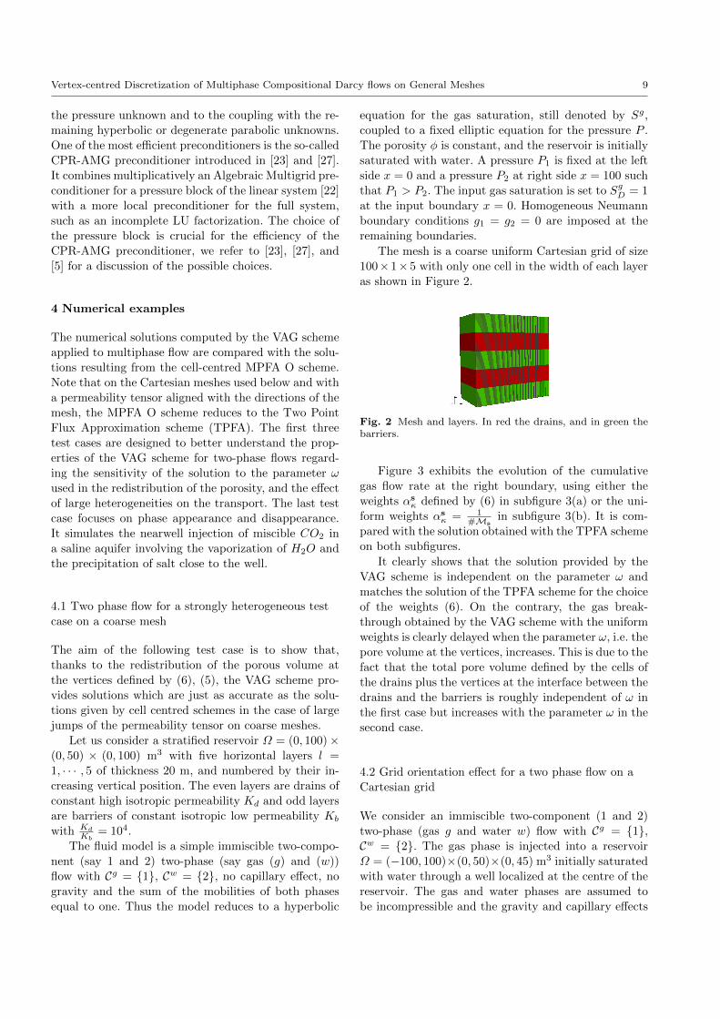
The mesh is a coarse uniform Cartesian grid of size

100×1×5 with only one cell in the width of each layer

as shown in Figure 2.

Fig. 2 Mesh and layers. In red the drains, and in green thebarriers.

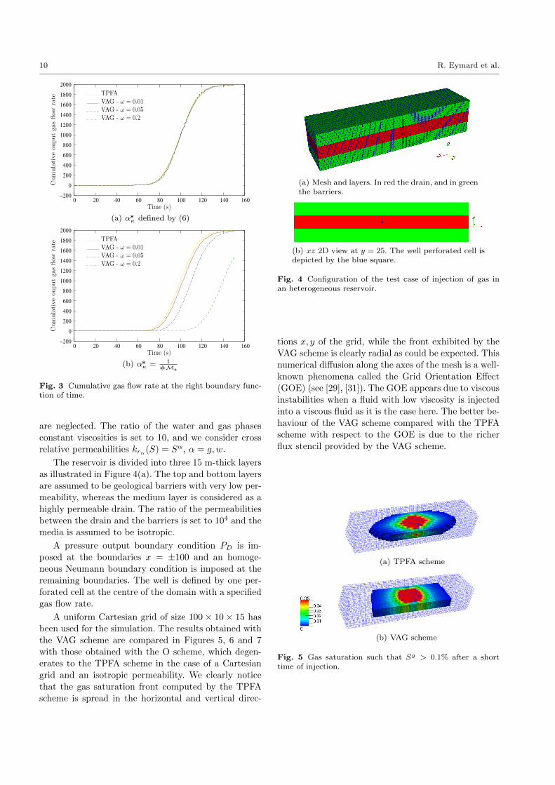
Figure 3 exhibits the evolution of the cumulative

gas flow rate at the right boundary, using either the

weights αsκ defined by (6) in subfigure 3(a) or the uni-

form weights αsκ = 1

#Msin subfigure 3(b). It is com-

pared with the solution obtained with the TPFA scheme

on both subfigures.

It clearly shows that the solution provided by the

VAG scheme is independent on the parameter ω and

matches the solution of the TPFA scheme for the choice

of the weights (6). On the contrary, the gas break-

through obtained by the VAG scheme with the uniform

weights is clearly delayed when the parameter ω, i.e. the

pore volume at the vertices, increases. This is due to the

fact that the total pore volume defined by the cells of

the drains plus the vertices at the interface between the

drains and the barriers is roughly independent of ω in

the first case but increases with the parameter ω in the

second case.

4.2 Grid orientation effect for a two phase flow on a

Cartesian grid

We consider an immiscible two-component (1 and 2)

two-phase (gas g and water w) flow with Cg = 1,Cw = 2. The gas phase is injected into a reservoir

Ω = (−100, 100)×(0, 50)×(0, 45) m3 initially saturated

with water through a well localized at the centre of the

reservoir. The gas and water phases are assumed to

be incompressible and the gravity and capillary effects

10 R. Eymard et al.

−200

0

200

400

600

800

1000

1200

1400

1600

1800

2000

0 20 40 60 80 100 120 140 160

Cum

ula

tive

ouput

gas

flow

rate

Time (s)

TPFA

VAG - ω = 0.2

VAG - ω = 0.01VAG - ω = 0.05

(a) αsκ defined by (6)

−200

0

200

400

600

800

1000

1200

1400

1600

1800

2000

0 20 40 60 80 100 120 140 160

Cum

ula

tive

ouput

gas

flow

rate

Time (s)

TPFAVAG - ω = 0.01VAG - ω = 0.05VAG - ω = 0.2

(b) αsκ = 1

#Ms

Fig. 3 Cumulative gas flow rate at the right boundary func-tion of time.

are neglected. The ratio of the water and gas phases

constant viscosities is set to 10, and we consider cross

relative permeabilities krα(S) = Sα, α = g, w.

The reservoir is divided into three 15 m-thick layers

as illustrated in Figure 4(a). The top and bottom layers

are assumed to be geological barriers with very low per-

meability, whereas the medium layer is considered as a

highly permeable drain. The ratio of the permeabilities

between the drain and the barriers is set to 104 and the

media is assumed to be isotropic.

A pressure output boundary condition PD is im-

posed at the boundaries x = ±100 and an homoge-

neous Neumann boundary condition is imposed at the

remaining boundaries. The well is defined by one per-

forated cell at the centre of the domain with a specified

gas flow rate.

A uniform Cartesian grid of size 100 × 10 × 15 has

been used for the simulation. The results obtained with

the VAG scheme are compared in Figures 5, 6 and 7

with those obtained with the O scheme, which degen-

erates to the TPFA scheme in the case of a Cartesian

grid and an isotropic permeability. We clearly notice

that the gas saturation front computed by the TPFA

scheme is spread in the horizontal and vertical direc-

(a) Mesh and layers. In red the drain, and in greenthe barriers.

(b) xz 2D view at y = 25. The well perforated cell isdepicted by the blue square.

Fig. 4 Configuration of the test case of injection of gas inan heterogeneous reservoir.

tions x, y of the grid, while the front exhibited by the

VAG scheme is clearly radial as could be expected. This

numerical diffusion along the axes of the mesh is a well-

known phenomena called the Grid Orientation Effect

(GOE) (see [29], [31]). The GOE appears due to viscous

instabilities when a fluid with low viscosity is injected

into a viscous fluid as it is the case here. The better be-

haviour of the VAG scheme compared with the TPFA

scheme with respect to the GOE is due to the richer

flux stencil provided by the VAG scheme.

(a) TPFA scheme

(b) VAG scheme

Fig. 5 Gas saturation such that Sg > 0.1% after a shorttime of injection.


(a) TPFA scheme

(b) VAG scheme

Fig. 6 Cut at z = 22.5 m - Gas saturation at the end of thesimulation.

(a) TPFA scheme

(b) VAG scheme

Fig. 7 Cut at y = 25 m - Gas saturation at the end of thesimulation.

4.3 Numerical diffusion and CPU time for a decoupled

two phase flow

We consider a simple immiscible two-component (say 1

and 2) two-phase (say gas (g) and water (w)) flow with

Cg = 1, Cw = 2, no capillary effect, no gravity

and the sum of the mobilities of both phases equal to

one. In such a case, the model reduces to a linear scalar

hyperbolic equation for the gas saturation denoted by

Sg coupled to an elliptic equation for the pressure P .

The simulation is done on the domain Ω = (0, 1)3 with

the permeability tensor Λ = I, a porosity φ = 1, and the

initial gas saturation Sg(x, 0) = 0. Let (x, y, z) denote

the Cartesian coordinates of x. We specify a pressure

P1 at the left side x = 0 and a pressure P2 at right

side x = 1 such that P1 > P2. Homogeneous Neumann

boundary conditions g1 = g2 = 0 are imposed at the

remaining boundaries. The input gas saturation is set

to SgD = 1 at the input boundary x = 0. The system

admits an analytical solution given by

P (x) = (P2 − P1) x+ P1,

and

Sg(x, t) =

1 if x 6 (P1 − P2) t,

0 else.

We consider two different grids for this test. The

first one is a uniform Cartesian grid of size 32×32×32.

The second grid is composed of 15266 tetrahedra. Both

meshes are extracted from the FVCA6 3D Benchmark

[21].

Figure 8 shows, for each grid, the gas saturation Sg

in function of the x–coordinate at the time of the sim-

ulation for which the gas has filled half of the reservoir.

We have plotted the analytical solution Sg and the dis-

crete solutions (xκ, Sgκ) for all cells κ ∈ M obtained

with the VAG and the MPFA O schemes. For the VAG

scheme we use the post-processed values,

Sgκ = (1− ω∑

s∈Vκ\VD

αsκ)Sgκ + ω

∑s∈Vκ\VD

αsκS

gs

deduced from the redistribution of the volumes defined

by (5)-(6) .

0

0.2

0.4

0.6

0.8

1

0 0.2 0.4 0.6 0.8 1

Sg

x

solutionO scheme

VAG - ω = 0.01VAG - ω = 0.3

(a) Hexahedral mesh

0

0.2

0.4

0.6

0.8

1

0 0.2 0.4 0.6 0.8 1

Sg

x

solutionO scheme

VAG - ω = 0.01

(b) Tetrahedral mesh

Fig. 8 Propagation in the horizontal direction of the gassaturation.

The results presented in Figure 8 clearly show that,

for each grid, the discrete solutions of both schemes in-

tersect the analytical solution at the point ( 12 ,

12 ), which

exhibits that the velocity of the flow is well approxi-

mated.

On Figure 8(a), the solutions of the VAG scheme

on the Cartesian grid is plotted for both ω = 0.01 and

12 R. Eymard et al.

ω = 0.3 (5). The value ω = 0.3 roughly corresponds

to match the pore volume of each vertex φs with the

pore volume of each surrounding cell φκ, κ ∈ Ms. As

expected, the choice ω = 0.3 leads to a slightly less

diffusive scheme than the VAG scheme with ω = 0.01.

We note also that the VAG scheme is slightly less diffu-

sive on such meshes than the MPFA O scheme (which

degenerates for Cartesian grids to the TPFA scheme).

On the other hand, for the tetrahedral mesh, we can

notice on Figure 8(b) that the VAG scheme is slightly

more diffusive than the MPFA O scheme. This has been

observed for both values of ω = 0.01 and 0.3.

Note also that for both type of meshes the conver-

gence of the VAG scheme has been obtained numeri-

cally for both ω = 0.01 and ω = 0.3.

In terms of CPU time a ratio of 15 is observed be-

tween the simulation time obtained with the MPFA O

scheme on the tetrahedral mesh and the VAG scheme

on the same mesh. This huge factor is due to the re-

duced size of the linear system obtained with the VAG

scheme after elimination of the cell unknowns compared

with the MPFA O scheme, both in terms of number of

unknowns (around five time less for the VAG scheme

than for the MPFA O scheme) and in terms of number

of non zero elements per line.

4.4 CO2 injection with dissolution and vaporization of

H2O and salt precipitation

This test case simulates the nearwell injection of CO2

in a saline aquifer. Due to the vaporization of H2O in

the gas phase, the water phase is drying in the nearwell

region leading to the precipitation of the salt dissolved

in the water phase. This may result in a reduction of

the nearwell permeability. This phenomenon could for

example explain the loss of injectivity observed in the

Tubaen saline aquifer of the Snohvit field in the Barents

sea where around 700000 tons of CO2 are injected each

year since 2008.

The model is a three phases three components com-

positional Darcy flow, with C = H2O,CO2, salt and

P = water(w), gas(g),mineral(m). It is assumed that

the H2O component can vaporize in the gas phase and

that the CO2 and salt components can dissolve in the

water phase. It results that Cw = H2O,CO2, salt,Cg = H2O,CO2, and Cm = salt. The mineral

phase is immobile with a null relative permeability kr,m =

0, and the water and gas phase relative permeabilities

kr,α are non decreasing functions of the reduced satu-

ration Sα = Sα

Sw+Sg , α = w, g.

kr,α(Sα) =

(Sα − Sr,α1− Sr,α

)eαif Sα ∈ [Sr,α, 1]

0 if Sα < Sr,α,

with ew = 5, eg = 2, Sr,w = 0.3 and Sr,g = 0. The

reference pressure is chosen to be the gas pressure P =

P g, and we set Pw = P g + Pc,w(Sw) with

Pc,w(Sw) = Pc,1 log( Sw − Sr,w

1− Sr,w

)− Pc,2,

for 1 ≥ Sw > Sr,w, where Pc,1 = 2.104 Pa, Pc,2 = 104

Pa. The thermodynamical equilibrium is modelled by

equilibrium constants Ki, i ∈ C such that

CgH2O= KH2O CwH2O

in presence of both phases w and g,

CwCO2= KCO2 C

gCO2

in presence of both phases w and g,

Cwsalt = Ksalt

in presence of both phases w and m.

The equilibrium constants will be considered fixed in

the range of pressure and temperature with the follow-

ing values KH2O = 0.025, KCO2 = 0.03 and Ksalt =

0.39 in kg/kg. With these assumptions, the flash Q =

flash(P,Z

)admits an analytical solution, independent

of the pressure P , and with entries Z in the two di-

mensional simplex (ZCO2 , Zsalt) |ZCO2 ≥ 0, Zsalt ≥0, 1 − ZCO2

− Zsalt ≥ 0. The solution is exhibited

Figure 9 where we have set E1 = (ECO2KCO2

, 0),

E2 = (ECO2 , 0), E3 = (DCO2 , 0), E4 = (0,Ksalt), E5

= (KCO2DCO2

,Ksalt),

with DCO2 =1−KH2O (1−Ksalt)

1−KH2O KCO2

,

and ECO2=

1−KH2O

1−KH2O KCO2

.

The 3D nearwell grids used for the simulation are

exhibited in Figure 10. The first step of the discretiza-

tion is to create a radial mesh, Figure 10(a), that is

exponentially refined down to the well boundary. This

nearwell radial local refinement is matched with the

reservoir Ω = (−15, 15)× (−15, 15)× (−7.5, 7.5) m3 us-

ing either hexahedra (see Figure 10(b)) or both tetra-

hedra and pyramids, (see Figure 10(c)). The radius of

the well is 10 cm and the radius of the radial zone is 5

m. The well is deviated by an angle of 20 degrees away

from the vertical axis z in the x, z plane. The hexahe-

dral grid has 42633 cells and the hybrid grid 77599 cells.


0

0.2

0.4

0.6

0.8

1

0 0.2 0.4 0.6 0.8 1E1

E3

E5

E4

g +m

m

E2

g

w

w +m

w + g +m

w + g

ZCO2

Zsalt

Fig. 9 Diagram of present phases in the space (ZCO2, Zsalt).

(a) exponentially re-fined radial mesh

(b) unstructured mesh with onlyhexahedra

(c) hybrid mesh with hexahedra,tetrahedra and pyramids

Fig. 10 Nearwell meshes.

The remaining of the data set and the boundary and

initial conditions are the following. The porosity is set

to φ = 0.2, and the permeability tensor Λ is homoge-

neous and isotropic equal to 1. 10−12 m2. The density

and the viscosity of the water phase are computed by

correlations function of P and Cw, and those of the

gas phase by linear interpolation in the pressure P , the

density of the mineral phase is fixed to ρm = 2173 kg/l.

Homogeneous Neumann boundary conditions are im-

posed on the top and bottom boundaries. Along the well

boundary we impose the pressure P (x, y, z) = Pwell −ρg ‖ g ‖ z, with Pwell = 300 10+5 Pa, the input phase

Sg = 1 and its composition CgCO2= 1, CgH2O

= 0. On

the lateral outer boundaries (resp. at initial time) the

following hydrostatic pressure is imposed P (x, y, z) =

P1−ρl ‖ g ‖ z, with P1 = Pwell−10+5 Pa, as well as the

following input (resp. initial) phase and its composition

Sw = 1, CwH2O= 0.84 and Cwsalt = 0.16.

The simulation time is fixed to 7 days in order to

obtain a precipitation of the mineral up to around half

of the radial zone. To avoid too small control volumes

in the nearwell region, the parameter ω has been chosen

in such a way that minκ∈M φk = mins∈V φs, leading in

our case to ω ∼ 0.4. The simulation with the O scheme

on the hybrid grid could not be obtained due to too

high memory requirement.

Figure 11 exhibits, for the two schemes and on both

grids, the rate of variation of the masses of CO2 and

of the mineral in the reservoir function of time. We can

notice that the VAG scheme solutions on both meshes

are almost the same and only slightly differ from the

O scheme solution. The oscillations observed in Figure

11(b) are a well-known phenomenon due to the appear-

ance of the mineral phase on each successive cells when

the salt reaches its maximum solubility.

Figure 12 exhibits the trajectory of the total mass

fraction Z in the simplex (ZCO2, Zsalt) function of time

for four cells κi, i = 1, · · · , 4. Starting from an initial

state given by a single water phase and ZCO2 = 0, the

mass of CO2 increases due to the injection. The CO2

is initially fully dissolved in the water phase, then the

gas phase appears and its mass fraction θg increases.

As long as CwSalt is roughly constant, the trajectory Z

is close to the line defined byZCO2 = (1− θg)CwCO2

+ θgCgCO2,

Zsalt = (1− θg)Cwsalt

since CwCO2and CgCO2

are both fixed by Cwsalt and the

thermodynamical equilibrium constants. Once the wa-

ter saturation Sw is close to the irreducible water satu-

ration Sr,w, the composition Cwsalt increases rapidly due

to the vaporization of H2O and the mineral phase ap-

pears. At the end of the simulation, it only remains the

CO2 component in the gas phase and the salt compo-

nent in the mineral phase and the trajectory ends on

the segment ZH2O = 0.

14 R. Eymard et al.

0

2

4

6

8

10

12

14

16

18

20

0 1 2 3 4 5 6 7

Time (day)

VAG - hexahedraO scheme - hexahedra

Variation

ofthemassofCO2

VAG - hybrid

(a) CO2

0

0.005

0.01

0.015

0.02

0.025

0.03

0.035

0.04

0.045

0 1 2 3 4 5 6 7

Variation

ofthemassof

mineral

Time (day)

VAG - hexahedraVAG - hybrid

O scheme - hexahedra

(b) Mineral

Fig. 11 Rate of variation of the mass of CO2 and of mineralin the reservoir function of time.

0

0.2

0.4

0.6

0.8

1

0 0.2 0.4 0.6 0.8 1

ZCO2

κ2κ3κ4

κ1

Zsalt

Fig. 12 Trajectory of Zκ for four cells κi, i = 1, · · · , 4 inthe space (ZCO2

, Zsalt). The four cells at all at z = −7 mand ordered according to their increasing distance to the wellaxis.

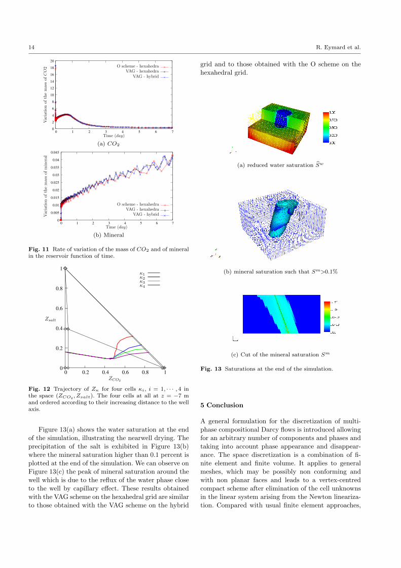
Figure 13(a) shows the water saturation at the end

of the simulation, illustrating the nearwell drying. The

precipitation of the salt is exhibited in Figure 13(b)

where the mineral saturation higher than 0.1 percent is

plotted at the end of the simulation. We can observe on

Figure 13(c) the peak of mineral saturation around the

well which is due to the reflux of the water phase close

to the well by capillary effect. These results obtained

with the VAG scheme on the hexahedral grid are similar

to those obtained with the VAG scheme on the hybrid

grid and to those obtained with the O scheme on the

hexahedral grid.

(a) reduced water saturation Sw

(b) mineral saturation such that Sm>0.1%

(c) Cut of the mineral saturation Sm

Fig. 13 Saturations at the end of the simulation.

5 Conclusion

A general formulation for the discretization of multi-

phase compositional Darcy flows is introduced allowing

for an arbitrary number of components and phases and

taking into account phase appearance and disappear-

ance. The space discretization is a combination of fi-

nite element and finite volume. It applies to general

meshes, which may be possibly non conforming and

with non planar faces and leads to a vertex-centred

compact scheme after elimination of the cell unknowns

in the linear system arising from the Newton lineariza-

tion. Compared with usual finite element approaches,


the VAG scheme has the ability to deal with highly het-

erogeneous media on coarse meshes due to its flexibility

in the definition of the porous volumes at the vertices.

The efficiency of our approach on complex meshes

and for complex compositional models is exhibited on

three phases three components models which simulate

the nearwell injection of miscible CO2 in a saline aquifer

taking into account the vaporization of H2O in the gas

phase as well a the deposition of the salt.

Acknowledgements This work was partially supported byGNR MoMAS.

References

1. Aavatsmark, I., Barkve, T., Boe, O., Mannseth, T.: Dis-cretization on non-orthogonal, quadrilateral grids for in-homogeneous, anisotropic media. Journal of computa-tional physics 127(1), 2–14 (1996)

2. Aavatsmark, I., Barkve, T., Boe, O., Mannseth, T.: Dis-cretization on unstructured grids for inhomogeneous,anisotropic media. part i: Derivation of the methods.SIAM Journal on Scientific Computing 19, 1700 (1998)

3. Aavatsmark, I., Eigestad, G., Mallison, B., Nordbotten,J.: A compact multipoint flux approximation methodwith improved robustness. Numerical Methods for Par-tial Differential Equations 24(5), 1329–1360 (2008)

4. Abadpour, A., Panfilov, M.: Method of negative satura-tions for modelling two phase compositional flows withoversaturated zones. Transport in porous media 79,2,197–214 (2010)

5. Achdou, Y., Bonneau, P., Masson, R., Quandalle, P.:Block preconditioning and multigrid solvers for linear sys-tems in reservoir simulations. In: European Conferenceon Mathematics of Oil Recovery ECMOR X (2006)

6. Agelas, L., Di Pietro, D., Droniou, J.: The g method forheterogeneous anisotropic diffusion on general meshes.ESAIM: Mathematical Modelling and Numerical Anal-ysis 44(04), 597–625 (2010)

7. Agelas, L., Di Pietro, D., Eymard, R., Masson, R.: Anabstract analysis framework for nonconforming approx-imations of diffusion on general meshes. InternationalJournal on Finite Volumes 7(1) (2010)

8. Agelas, L., Guichard, C., Masson, R.: Convergence offinite volume mpfa o type schemes for heterogeneousanisotropic diffusion problems on general meshes. Inter-national Journal on Finite Volumes 7(2) (2010)

9. Angelini, O.: Etude de schemas numeriques pour lesecoulements diphasiques en milieu poreux deformablepour des maillages quelconques: application au stockagede dechets radioactifs. Ph.D. thesis, Universite Paris-EstMarne-la-Vallee (2010)

10. Aziz, K., Settari, A.: Petroleum Reservoir Simulation.Applied Science Publishers (1979)

11. Bourgeat, A., Jurak, M., Smai, F.: Two phase partiallymiscible flow and transport in porous media; applicationto gas migration in nuclear waste repository. Computa-tional Geosciences 13,1, 29–42 (2009)

12. Cao, H.: Development of techniques for general purposesimulators. Ph.D. thesis, University of Stanfords (2002)

13. Coats, K.H.: An equation of state compositional model.In: SPE Reservoir Simulation Symposium Journal, pp.363–376 (1980)

14. Coats, K.H.: Implicit compositional simulation of single-porosity and dual-porosity reservoirs. In: SPE Sympo-sium on Reservoir Simulation (1989)

15. Edwards, M., Rogers, C.: A flux continuous scheme forthe full tensor pressure equation. in prov. of the 4th eu-ropean conf. on the mathematics of oil recovery, 1994

16. Edwards, M., Rogers, C.: Finite volume discretizationwith imposed flux continuity for the general tensor pres-sure equation. Computational Geosciences 2(4), 259–290(1998)

17. Eymard, R., Gallouet, T., Herbin, R.: Discretisation ofheterogeneous and anisotropic diffusion problems on gen-eral non-conforming meshes, sushi: a scheme using sta-bilisation and hybrid interfaces. IMA J. Numer. Anal.30(4), 1009–1043 (2010)

18. Eymard, R., Guichard, C., Herbin, R.: Small-stencil 3dschemes for diffusive flows in porous media. ESAIM:Mathematical Modelling and Numerical Analysis 46,265–290 (2010)

19. Eymard, R., Guichard, C., Herbin, R.: Benchmark 3d: thevag scheme. In: J. Fort, J. Furst, J. Halama, R. Herbin,F. Hubert (eds.) Finite Volumes for Complex Applica-tions VI – Problems and Perspectives, vol. 2, pp. 213–222.Springer Proceedings in Mathematics (2011)

20. Eymard, R., Guichard, C., Herbin, R., Masson, R.: Ver-tex centred discretization of two-phase darcy flows ongeneral meshes. In: Proceedings of the SMAI conference2011. ESAIM Proceedings (submitted 2011)

21. Eymard, R., Henry, G., Herbin, R., Hubert, F., Klofkorn,R., Manzini, G.: Benchmark 3d on discretization schemesfor anisotropic diffusion problem on general grids. In:J. Fort, J. Furst, J. Halama, R. Herbin, F. Hubert (eds.)Finite Volumes for Complex Applications VI – Problemsand Perspectives, vol. 2, pp. 95–265. Springer Proceed-ings in Mathematics (2011)

22. Henson, V., Yang, U.: Boomeramg: A parallel algebraicmultigrid solver and preconditioner. Applied NumericalMathematics 41, 155–177 (2002)

23. Lacroix, S., Vassilevski, Y.V., Wheeler, M.F.: Decouplingpreconditioners in the implicit parallel accurate reservoirsimulator (ipars). Numerical Linear Algebra with Appli-cations 8, 537–549 (2001)

24. Michelsen, M.L.: The isothermal flash problem. part i:Stability. Fluid Phase Equilibria 9, 1–19 (1982)

25. Peaceman, D.W.: Fundamentals of Numerical ReservoirSimulations. Elsevier (1977)

26. Quandalle, P., Savary, D.: An implicit in pressure andsaturations approach to fully compositional simulation.In: SPE Reservoir Simulation Symposium, 18423 (1989)

27. Scheichl, R., Masson, R., Wendebourg, J.: Decouplingand block preconditioning for sedimentary basin simu-lations. Computational Geosciences 7, 295–318 (2003)

28. Thomas, G.W., Thurnau, D.H.: Reservoir simulation us-ing and adaptive implicit method. Soc. Pet. Eng. Journal19 (1983)

29. Vinsome, P., Au, A.: One approach to the grid orientationproblem in reservoir simulation. Old SPE Journal 21(2),160–161 (1981)

30. Whitson, C.H., Michelsen, M.L.: The negative flash.Fluid Phase Equilibria 53, 51–71 (1989)

31. Yanosik, J.L., McCracken, T.A.: A nine-point, finite-difference reservoir simulator for realistic prediction ofadverse mobility ratio displacements. Old SPE Journal19(4), 253–262 (1979)

Documents

Vertex-centred Discretization of Multiphase Compositional