Embed Size (px)
Citation preview
Naval Research Laboratory Monterey, CA 93943-5502
NRL/MR/7531-99-7240
Vertical Correlation Functions for Temperature and Relative Humidity Errors
RICHARD FRANKE
Atmospheric Dynamics & Prediction Branch Marine Meteorology Division
January 1999
Approved for public release; distribution unlimited.
DTIC QUALEnr INSPECTED
REPORT DOCUMENTATION PAGE Form Approved OMB No. 0704-0188
Public reporting burden for this collection of information is estimated to average 1 hour per response, including the time for reviewing instructions, searching existinq data sources, gathering and maintaining the data needed, and completing and reviewing the collection of information. Send comments regarding this burden or any other aspect of this collection of information, including suggestions for reducing this burden, to Washington Headquarters Services, Directorate for Information Operations and Reoorts 1215 Jefferson Davis Highway, Suite 1204, Arlington, VA 22202-4302, and to the Office of Management and Budget, Paperwork Reduction Project (0704-0188) Washington DC 20503
1. Agency Use Only (Leave Blank). 2. Report Date. January 1999
3. Report Type and Dates Covered. Final
Title and Subtitle. Vertical Correlation Functions for Temperature and Relative Humidity Errors
Author(s). Richard Franke
7. Performing Organization Name(s) and Address(es). Naval Research Laboratory Marine Meteorology Division Monterey, CA 93943-5502
8. Sponsoring/Monitoring Agency Name(s) and Address(es). Office of Naval Research Arlington, VA 22217-5660
11. Supplementary Notes.
5. Funding Numbers. PE 0602435N PN R3591
Performing Organization Reporting Number. NRL/MR/7531--99-7240
10. Sponsoring/Monitoring Agency Report Number.
12a. Distribution /Availability Statement. Approved for public release; distribution unlimited
12b. Distribution Code.
13. Abstract (Maximum 200 words).
This report gives the details and results of any investigation into the properties of the temperature and relative humidity errors from the Navy Operational Global Atmospheric Prediction System for a four-month period from March-June 1998. The spatial covariance data for temperature and for relative humidity was fit using eight different approximation functions/weighting methods. From these, two were chosen as giving good estimates of the parameters and variances of the prediction and observation errors and were used in further investigations. The vertical correlation between temperature errors at different levels and relative humidity errors at different levels was approximated using a combination of functional fitting and transformation of the pressure levels. The cross-covariance between temperature and relative humidity errors at various pressure levels were approximated in two ways: (1) by directly computing and approximating the cross- coVariance data, and (2) by approximating variance of the difference of normalized data. The latter led to more consistent results. There are numerous figures illustrating the results obtained and tables give the pertinent data.
14. Subject Terms. Covariance functions; Temperature error statistics; Relative humidity error statistics Temperature/humidity error correlation; NOGAPS
17. Security Classification of Report.
UNCLASSIFIED
NSN 7540-01-280-5500
18. Security Classification of This Page. UNCLASSIFIED
19. Security Classification of Abstract. UNCLASSIFIED
15. Number of Pages. 78
16. Price Code.
20. Limitation of abstract
Same as report
Standard Form 298 (Rev. 2-89) Prescribed by ANSI Std. Z39-18 298-102
CONTENTS
1. Introduction 1
2. Covariance Functions for Temperature and Relative Humidity 3
3. Estimation of Cross-Correlation of Temperature and Relative Humidity Errors by Direct Computation 8
4. Estimation of Cross-Correlation of Temperature and Relative Humidity Errors Through a Differencing Approach 10
5. Summary and Conclusions 13
Figures '. '. 15
Appendix .........59
Reference :........;. .69
in
ACKNOWLEDGEMENT
This research was conducted while the author was working for Naval Research
Laboratory/Monterey during FY98, supported under Program Element 0602435N. The
author expresses his thanks to Ed Barker, who made the arrangements, and Nancy Baker,
Roger Daley, and Andrew Van Tuyl, all of whom contributed to the effort by supplying
data and many useful comments. Formatting and editing of this manuscript was done by
Soheila Judy.
IV
1. Introduction
Plans for increasing the vertical resolution of the Navy Operational Global
Atmospheric Prediction System (NOGAPS) used by Fleet Numerical Meteorological and
Oceanographic Center require that the covariance structure for temperature and relative
humidity errors be modeled more accurately. This report details an investigation into the
statistical properties of the innovation data for these quantities. For this purpose a four
month time history of the data (March through June 1998, with the exception of one day,
March 27 at 00 UTC) was used, independently for times 00 UTC and 12 UTC. All valid
data from longitude 70° to 130° west and 25° to 55° north were used. Some preliminary
computations were carried out using a two' month history, but it was quickly determined
that data for the four month period led to binned data that seemed more consistent in that
the points have less scatter and can be better fit by a curve. This was less apparent at the
very lowest and highest levels, but at intermediate levels was consistently true. Such a
long period may obscure seasonal effects, and this will need to be investigated if such
details are to be incorporated into the system.
Previous work that investigates the cross-correlation of temperature and relative
humidity errors has been based on the "NMC method" (Parrish and Derber, 1992). There
the idea is to use the 24 and 48 hour forecasts to estimate the prediction error, assuming
that error growth is linear for that period of time. For vertical temperature error
correlations ECMWF has found a close agreement between this method and those
derived from innovation data (Courtier, et al, 1993). Steinle and Seaman (1995) also
used the "NMC method" to estimate the cross-correlation between temperature and
relative humidity.
The methods employed here are very much like those used previously by the
investigator (see Franke, 1998) and others. The temperature and relative humidity
innovation data were averaged at each level for each station over the 122 days. The mean
values were then subtracted from the innovation data. Then the raw covariance data were
formed and summed into bins of size 0.01 radians, keeping a count of the number of
terms. True radian distance on the sphere was used. Use of great circle distance poses a
potential difficulty with positive definiteness of the spatial covariance function
approximation, but it is thought to not pose a problem over regions of the size
contemplated. Experiments were carried out using several different forms of the
covariance function approximation and different weights for the squared residuals of the
binned data. Complete details of all results are not given here, but sufficient data to
indicate the nature of the results and reasons for the choices made are given.
The quantities measured by radiosondes are temperature and relative humidity
(Federal Meteorological Handbook No. 3, OFCM, 1997). The data supplied from
NOGAPS are the pressure p, predicted temperature T, and predicted specific humidity
Q. In the data file along with the NOGAPS data is the observed temperature Tg and
observed dewpoint depression D0 (which is actually reported), along with the quality
control flags. Using the formulas given by (OFCM, 1997), the observed value of relative
humidity is retrieved as follows: dewpoint temperature Td = T0— D0, observed vapor
< «TV > pressure e = cexp b + TdJ
, saturation vapor pressure es =cexp , and finally
e observed relative humidity uo = —. Here a, h, and c are constants,
e,
a = 17.502, b = 240.97° K, c = 6.1121 mb. It is assumed that these calculations reverse
those that obtained D0 from uo. If not, the relative humidity may be contaminated by
the observation error in T0. Similar formulas allow the calculation of the predicted value
of relative humidity from the predicted values of temperature, specific humidity, and *
Qp ,. , rp pressure p: mixing ratio r = —, predicted vapor pressure e =
\-Qp r + 0.622
saturation vapor pressure at the predicted temperature, es = cexp , and predicted
e relative humidity u -—, where a, b, and c are as before.
As we will see later, the independence of the observation errors for temperature and
relative humidity is questionable. Whether the values were cross contaminated from the
above operations, or whether the relative humidity observation error is somehow
dependent on temperature measurement errors is unknown.
2. Covariance functions for temperature and relative humidity
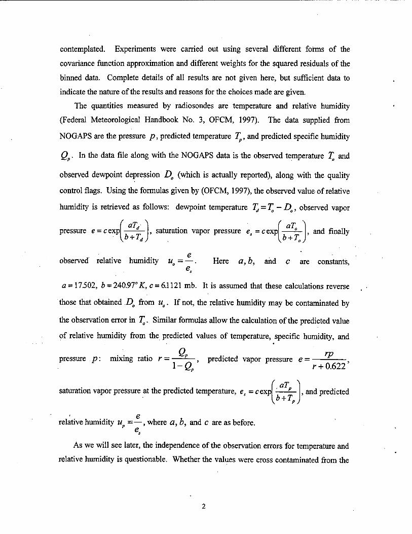
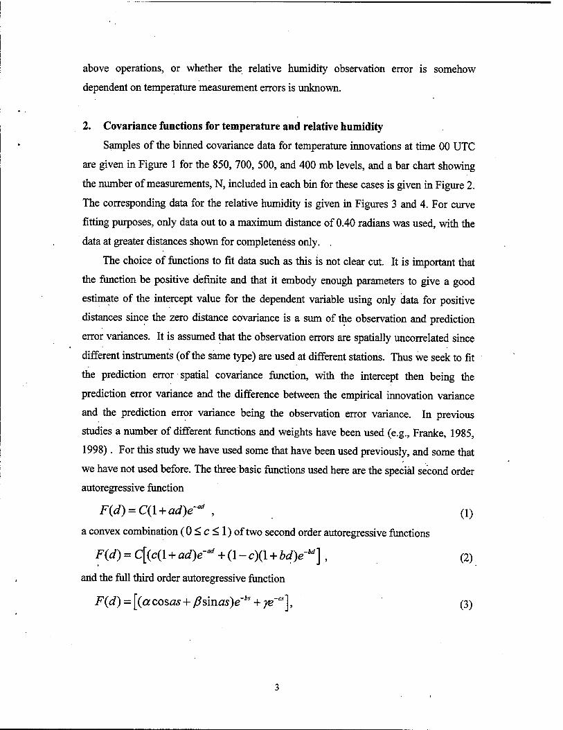
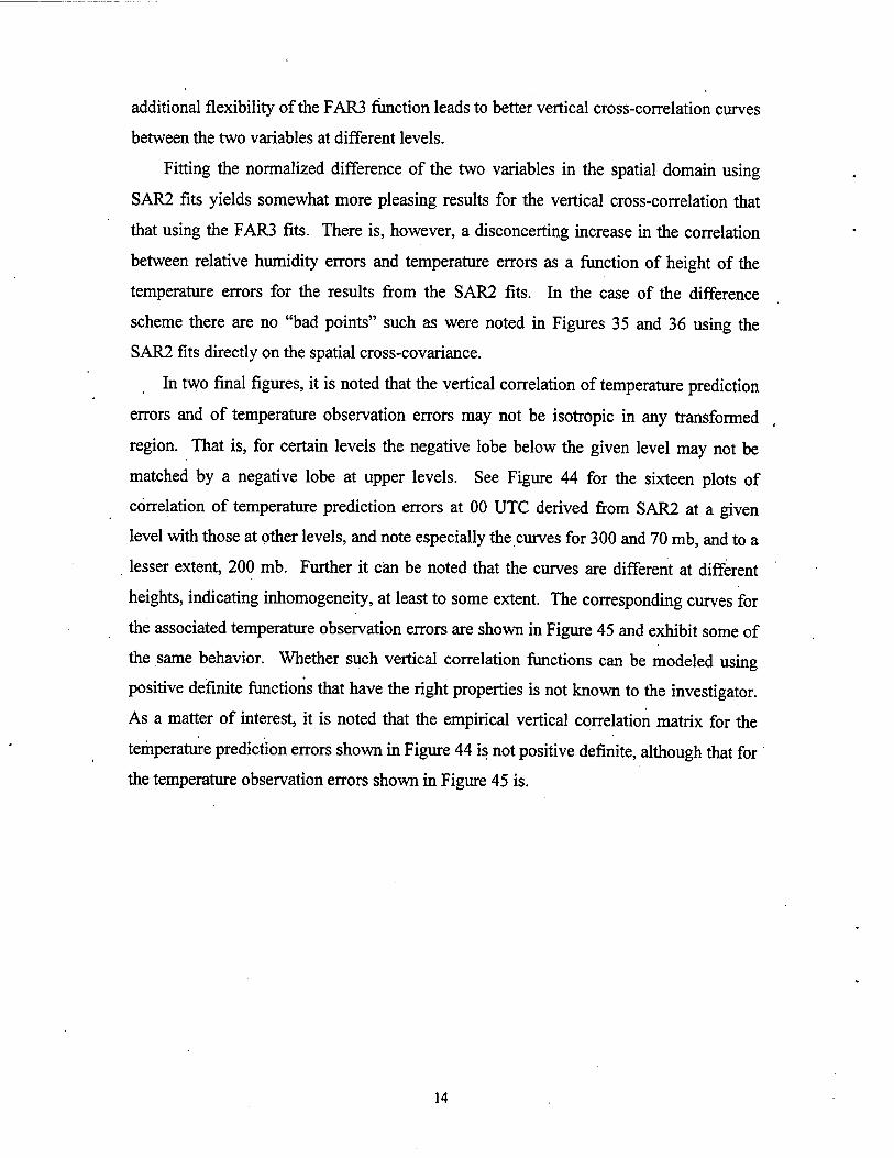
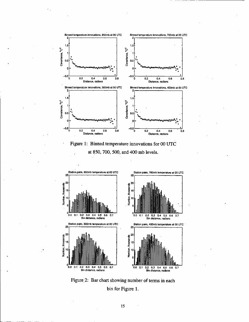
Samples of the binned covariance data for temperature innovations at time 00 UTC
are given in Figure 1 for the 850, 700, 500, and 400 mb levels, and a bar chart showing
the number of measurements, N, included in each bin for these cases is given in Figure 2.
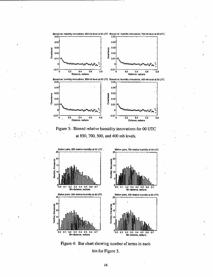
The corresponding data for the relative humidity is given in Figures 3 and 4. For curve
fitting purposes, only data out to a maximum distance of 0.40 radians was used, with the
data at greater distances shown for completeness only. .
The choice of functions to fit data such as this is not clear cut. It is important that
the function be positive definite and that it embody enough parameters to give a good
estimate of the intercept value for the dependent variable using only data for positive
distances since the zero distance covariance is a sum of the observation and prediction
error variances. It is assumed that the observation errors are spatially uncorrelated since
different instruments (of the same type) are used at different stations. Thus we seek to fit
the prediction error spatial covariance function, with the intercept then being the
prediction error variance and the difference between the empirical innovation variance
and the prediction error variance being the observation error variance. In previous
studies a number of different functions and weights have been used (e.g., Franke, 1985,
1998). For this study we have used some that have been used previously, and some that
we have not used before. The three basic functions used here are the special second order
autoregressive function
F{d) = C{\ + ad)ead , (1)
a convex combination (0 < c < 1) of two second order autoregressive functions
F(d) = C[(c(l + ad)e~ad + (1 - c){\ + bd)ebd] , (2)
and the full third order autoregressive function
F(d) = [(a cosas + ßsmas)e~bs + ye'"], (3)
(3b2-a2-c2)ac _ (b2-3a2-c2)bc -2(b2+a2)ab where a = , ß = ,/ = ,with
o do
S=(3b2-a2-c2)ac-2(b2 +a2)ab.
Function (1) has been used extensively by the investigator and others. Note that
function (2) was inspired by Mitchell, et al. (1990), where a sum of special third order
autoregressive functions were used (but with specified weights and relation between
constants in the exponential). Function (3) was chosen because it has more parameters
and embodies two different exponential decay rates, giving considerably more flexibility
than function (1), and with a different connection between the exponential decay terms
than that of function (2). All nonlinear least squares fits were computed using the
standard minimization function finins in Matlab®, which uses a Nelder-Mead simplex
algorithm. All nonlinear minimization routines are sensitive to the initial guess, and
some effort was expended in trying different initial guesses.
Table 1 gives a list of the functions and weights we have used to fit the temperature
and relative humidity innovations.
Ref# weight F 'unctio
1 N, d<0.40 (1)
2 N, d<0.20 0)
3 VN, d<0.40 (1)
4 l,fl?<0.40 (1)
5 N, d<0.40 (2)
6 N, d<0.20 (2)
7 VN, d<0.40 (2)
8 N, d<0.40 (3)
special second order AR, N -weighted (S2W1)
special second order AR, limited distance (S2W2)
special second order AR, 4N -weighted (S2W3)
special second order AR, equi-weighted (S2W4)
sum of two SAR2s, N -weighted (SS2W1)
sum of two SAR2s, limited distance (SS2W2)
sum of two SAR2s, VF-weighted (SS2W3)
Full third order AR, N -weighted (F3W1)
Table 1: Fitting functions and weighting for spatial least squares fits
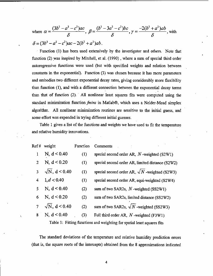
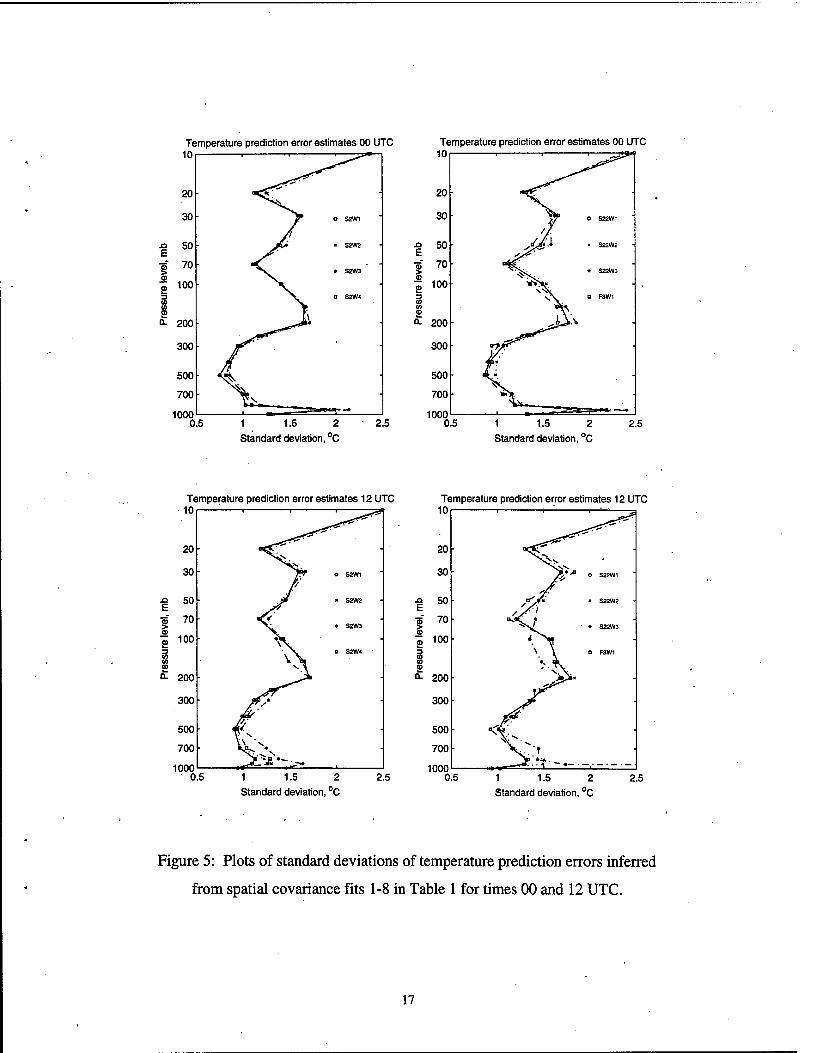
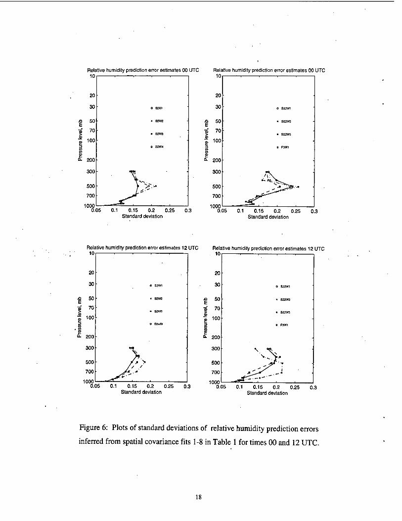
The standard deviations of the temperature and relative humidity prediction errors
(that is, the square roots of the intercepts) obtained from the 8 approximations indicated
in Table 1 are shown graphically for various levels at the two times in Figures 5 and 6.
Two things are striking: The general consistency of the results for the special second
order autoregressive fits (especially for temperature) and to a lesser extent the overall
consistency when some non-equal weighting is applied to the binned data, and the rather
different results obtained when using equal weighting.
The difficulties in obtaining appropriate approximations to the intercept (and hence
the variance of the prediction error) is a long-standing problem. In some sense the data
for short distances is most critical to defining that value, but on the other hand the amount
of data is very much less (as seen in Figure 2). Of course, this goes hand-in-hand with a
suitable assumption for the local behavior of the spatial covariance function for short
distances. As in previous work (Franke, 1998), it is felt here that some form of non-equal
weighting for the data is appropriate. The choice is not clear-cut, and somewhat
arbitrarily I have decided to use the weighting of Ref#l, weighting of the squared
residuals by the number of the data collected in the bin. Likewise I have decided to
pursue further investigations using only two fitting functions with that weighting, the
special second order autoregressive function and the full third order autoregressive
function. These will be referred to herafter as SAR2 and FAR3, respectively. It is
presently unknown what restrictions on the parameters will guarantee that the full third
order autoregressive function is positive definite in two dimensions, but the additional
parameters and flexibility available will allow some different behavior by the
approximating function for small distances. The FAR3 will also be used for the vertical
correlation approximations.
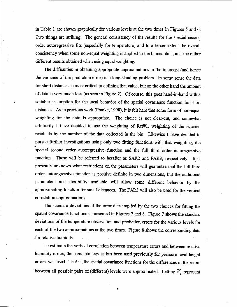
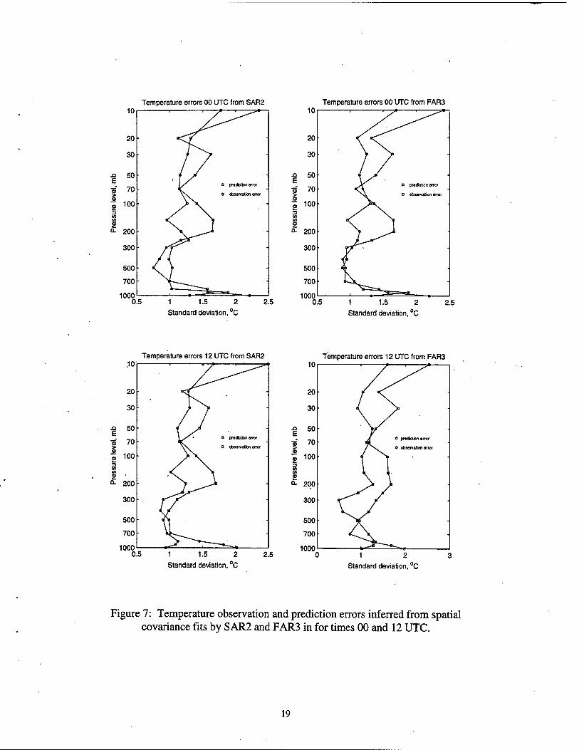
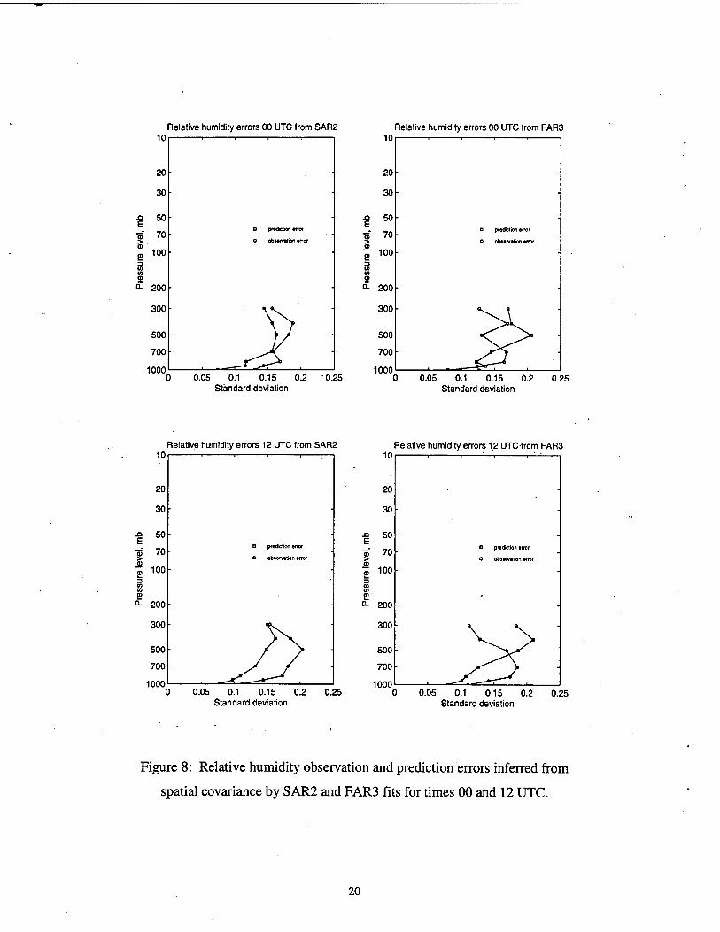
The standard deviations of the error data implied by the two choices for fitting the
spatial covariance functions is presented in Figures 7 and 8. Figure 7 shows the standard
deviations of the temperature observation and prediction errors for the various levels for
each of the two approximations at the two times. Figure 8 ■ shows the corresponding data
■for relative humidity.
To estimate the vertical correlation between temperature errors and between relative
humidity errors, the same strategy as has been used previously for pressure level height
errors was used. That is, the spatial covariance functions for the differences in the errors
between all possible pairs of (different) levels were approximated. Letting V. represent
the error of the quantity in question (temperature, or relative humidity), we estimate
var(F).-^). Then, since var(Fy -^) = var(^.)-2c6v(Fy,F;) + var(^), we
obtain
oov(VjVi) = far(Vj) + varTO- var^- - F})) (4)
Having estimated each of the quantities on the right side of Eq. (4) by approximating the
spatial covariance function for the quantity, we are able to obtain the vertical corvariance.
I The vertical correlation is then corty^V^) = cov(F;,)^) / (vaifJ^.) var(fQ)2.
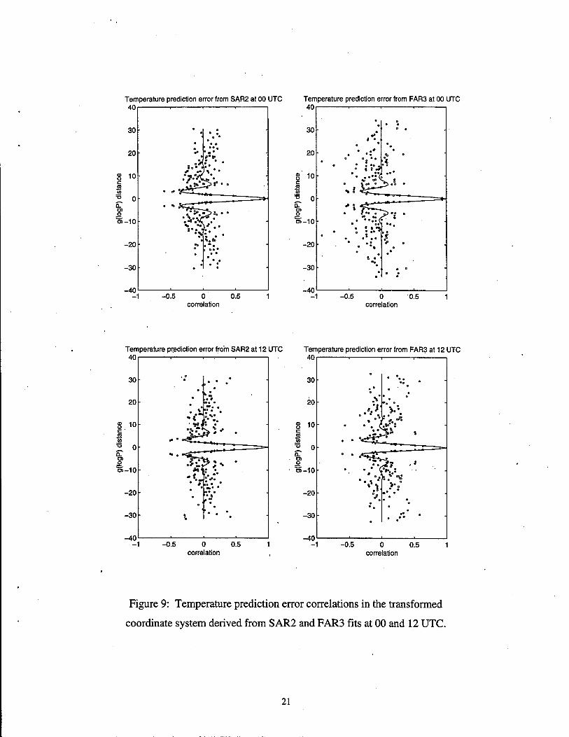
It is desirable that the vertical correlation functions be expressed in a stationary
isotropic form. In an attempt to achieve this, the simultaneous fit and transformation of
the vertical coordinate that was used by Franke (1998) was applied to these eight cases
for both prediction and observation error. Because there is appreciable negative
correlation at short distances, the full autoregressive function of order three given by Eq.
(3) was used. After translation of the values to the new coordinate system, the resulting
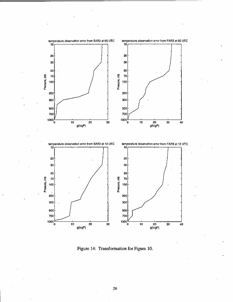
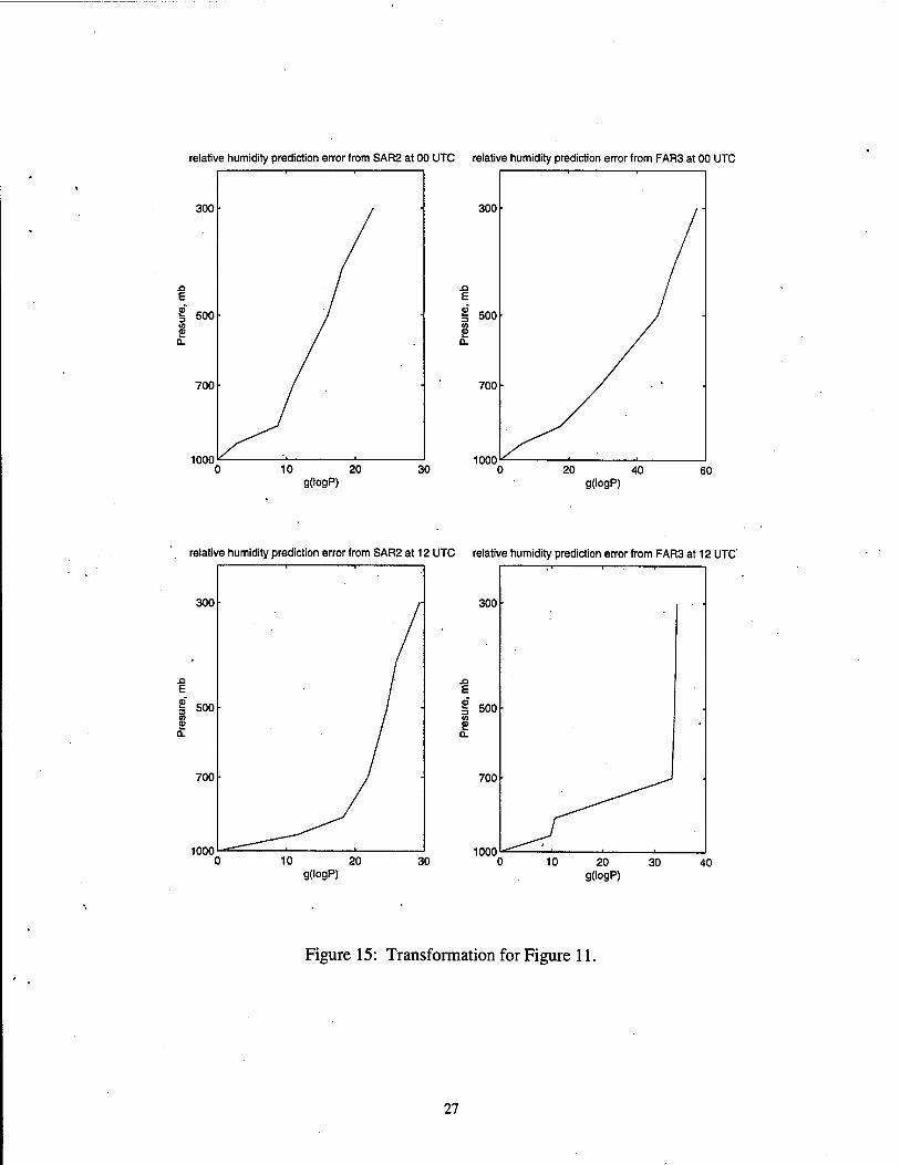
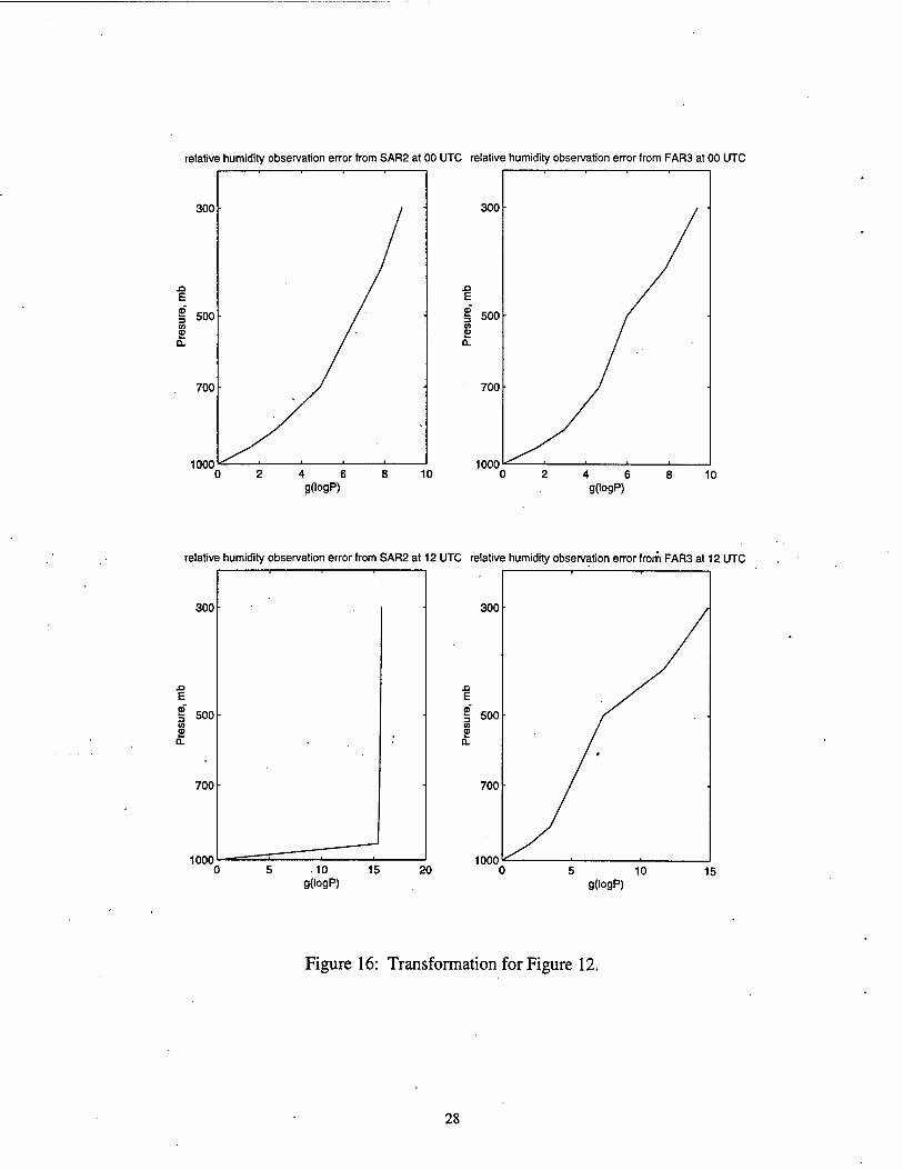
approximations, along with the correlation points, are shown in Figures 9-12. The
transformations generated for each of the approximations are shown in Figure 13-16.
The previous application (to height error correlations) generated considerable
improvement in terms of reducing the scatter and making the data look reasonably
coherent when viewed as isotropic in the transformed coordinate, however we see less of
this in Figures 9-12. At short distances the temperature prediction errors (Figure 9) are fit
well, however the relative humidity prediction errors (Figure 11) are not so well fit,
especially at 12 UTC. The situation is somewhat reversed with the observation errors,
where the fit is generally better for the relative humidity observation error (Figure 12)
than that for the relative humidity prediction error (Figure 10). The use of the full third
order autoregressive function for the vertical correlation approximation induces some
negative lobes in the approximation for the temperature prediction error and the relative
humidity observation error. Generally the approximating correlation functions for
temperature observation errors appear to be quite narrow, indicating the vertical errors
are nearly uncorrelated. It is noted that the transformations associated with some fits
(Figures 15 lower right and 16 lower left) both show extreme deformation between
certain points. It is also noted that some of the correlation values obtained through the
FAR3 fits are larger than one, although this is obscured by Figure 10 (upper right)
because the extent of the axis for the figure does not include the two points near
"correlation value" 1.3. There is no such occurrence with SAR2.
While some interesting things can be seen by looking at Figures 9-16, the more
realistic view comes by observing the fit to the correlation points and how the translation
affects the correlation curve approximation. For this purpose there are sixteen figures
that show the correlation curves mapped back to the log-pressure coordinate. The sixteen
figures (Figures 17-32) correspond to the sixteen subfigures of Figures 8-12. The order
the figures corresponds to the curves within each of Figures 8-12 from left to right, top to
bottom. In each of Figures 17-32, the four subfigures show a separated subset of the
correlation curves for correlation of the indicated error between pressure levels. The
label indicates the correlation curve for the error at that level with other levels. Also
shown in each figure are the data points giving the empirical correlation as computed by
the indicated method for the particular error and time. It is noted that .for purposes of
computing the correlation curves the transformation between levels was obtained by
piecewise linear interpolation. The figures can be perused at length, and yield
considerable information about the approximate behavior of the vertical correlation
functions for temperature and relative humidity prediction and observation error. The
general conclusion is much the same as was observed in Figures 8-16. The curves are
generally well-behaved for all cases.except those corresponding to Figures 15 lower right
and 16 lower left. The corresponding curves are shown in Figures 28 and 31,
respectively. Unfortunately, these two cases cut across both fitting methods, so that a
clear choice of fitting method does not appear here.
The correlation distance parameter is of interest. For function (1) this is the
reciprocal of the parameter a, while in function (3), there are two similar parameters, b
and c. The correlation distance is generally a measure of the distance at which the
function decays by a certain amount1, but for (3) the term is taken to mean the larger of
the reciprocals of b and c. Plots of the correlation distance parameters are given in
1 In this and previous papers the investigator uses decay to exp(-l) of the maximum value, but others have used decay to 0.5 of the maximum value.
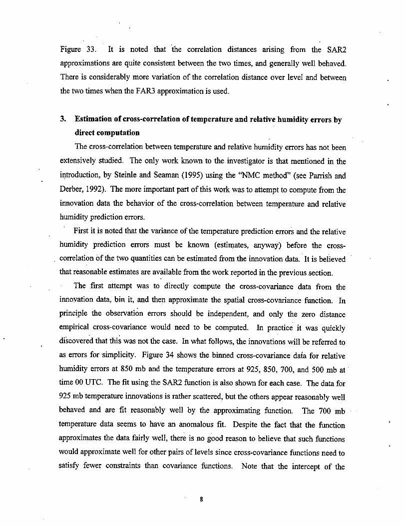
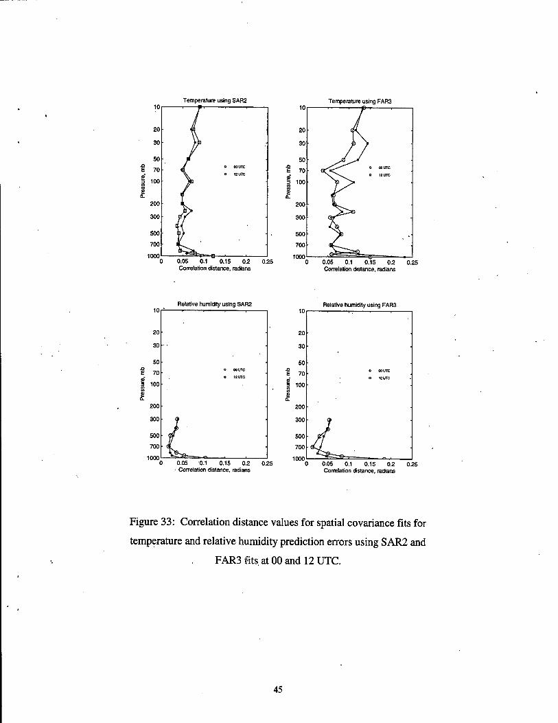
Figure 33. It is noted that the correlation distances arising from the SAR2
approximations are quite consistent between the two times, and generally well behaved.
There is considerably more variation of the correlation distance over level and between
the two times when the FAR3 approximation is used.
3. Estimation of cross-correlation of temperature and relative humidity errors by
direct computation
The cross-correlation between temperature and relative humidity errors has not been
extensively studied. The only work known to the investigator is that mentioned in the
introduction, by Steinle and Seaman (1995) using the "NMC method" (see Parrish and
Derber, 1992). The more important part of this work was to attempt to compute from the
innovation data the behavior of the cross-correlation between temperature and relative
humidity prediction errors.
First it is noted that the variance of the temperature prediction errors and the relative
humidity prediction errors must be known (estimates, anyway) before the cross-
correlation of the two quantities can be estimated from the innovation data. It is believed
that reasonable estimates are available from the work reported in the previous section.
The first attempt was to directly compute the cross-covariance data from the
innovation data, bin it, and then approximate the spatial cross-covariance function. In
principle the observation errors should be independent, and only the zero distance
empirical cross-covariance would need to be computed. In practice it was quickly
discovered that this was not the case. In what follows, the innovations will be referred to
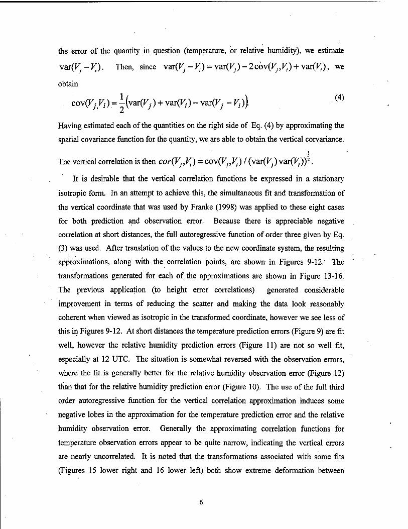
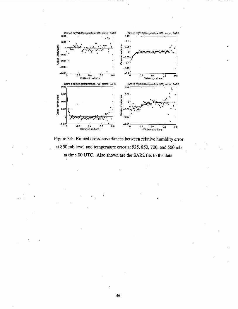
as errors for simplicity. Figure 34 shows the binned cross-covariance data for relative
humidity errors at 850 mb and the temperature errors at 925, 850, 700, and 500 mb at
time 00 UTC. The fit using the SAR2 function is also shown for each case. The data for
925 mb temperature innovations is rather scattered, but the others appear reasonably well
behaved and are fit reasonably well by the approximating function. The 700 mb
temperature data seems to have an anomalous fit. Despite the fact that the function
approximates the data fairly well, there is no good reason to believe that such functions
would approximate well for other pairs of levels since cross-covariance functions need to
satisfy fewer constraints than covariance functions. Note that the intercept of the
approximating function misses the value at zero distance, in each case, by a nontrivial
amount. Perusal of other pairs of levels also exhibit apparent additional correlated error
at zero distance. Whether this error is indeed due to correlated observation error, or
whether it is contamination of the innovation values for relative humidity when
calculated from predicted specific humidity and observed dewpoint depression is
unknown. In any case, it cannot be ignored!
Because most of the software was readily available, it was decided to approximate
the directly computed cross-covariance data using both the SAR2 fit and the FAR3 fit.
Using the intercepts of these approximations, the cross-covariance matrix for zero
distances between the 16 temperature levels and the 7 relative humidity levels was
computed, and hence the vertical cross-correlation matrix for temperature and relative
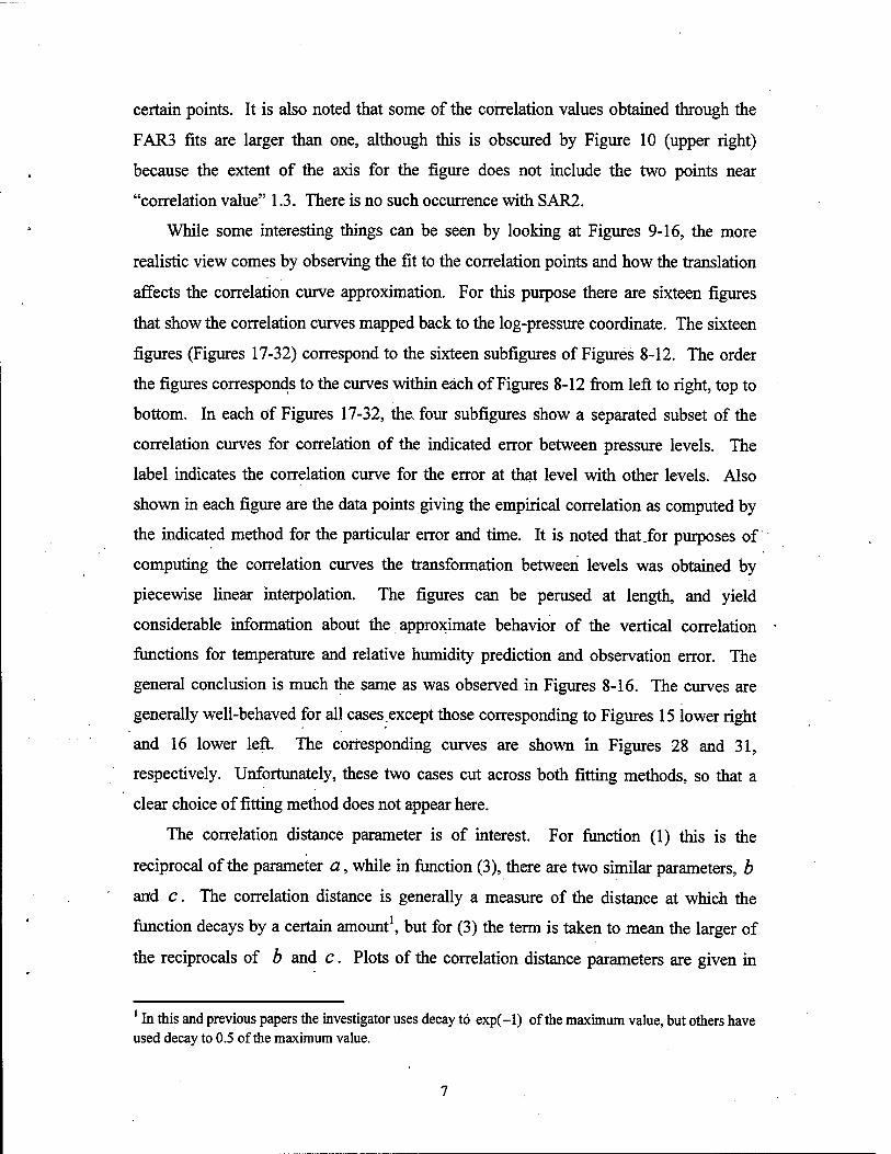
humidity. The seven figures showing the correlation between relative humidity error and
temperature errors at various heights at time 00 UTC are shown in Figure 35, as derived
from the SAR2 fits. Most notable is the strong negative correlation between temperature
errors and relative humidity errors at the same level up to 850 mb, and lesser negative
correlation at higher levels. Smaller amounts of data suggest one should might be
suspicious about the correlations between relative humidity error at 1000 mb and
temperature error at the upper levels. Perusal of the fits to the cross-covariance data for
relative humidity error at 1000 mb and temperature error at 200 mb and above show that
in most cases the fits do not seem unreasonable, however. The corresponding plots for
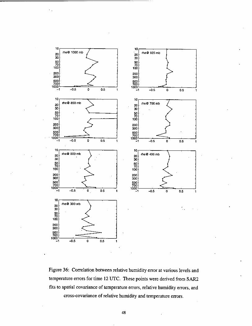
the cross-correlation data derived from the SAR2 fits at 12 UTC are shown in Figure 36.
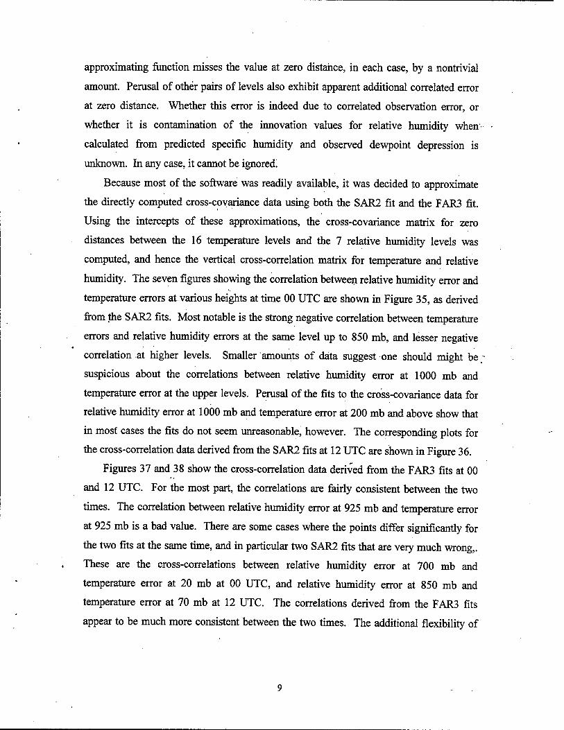
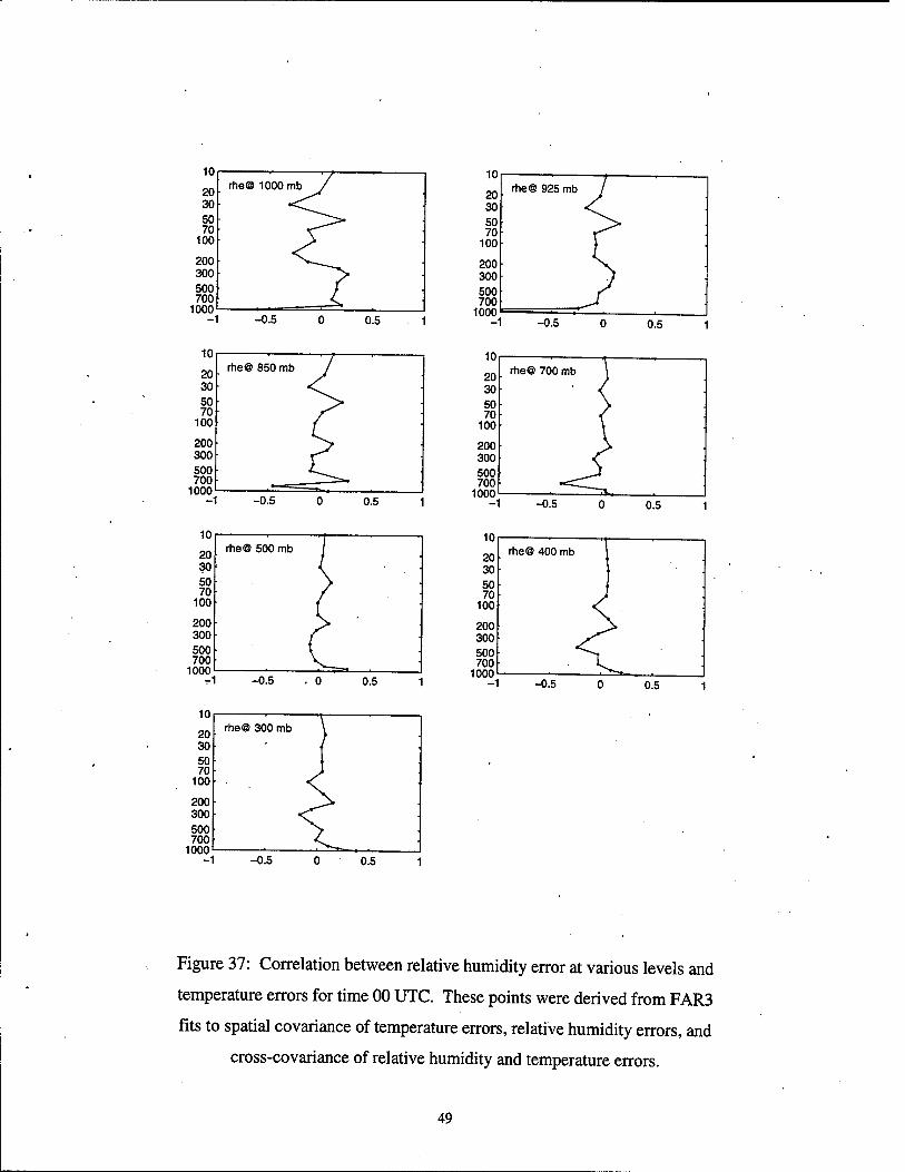
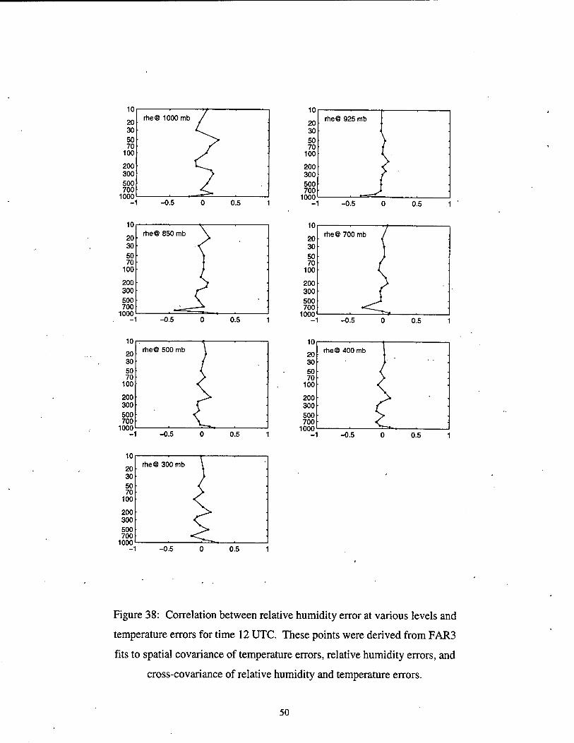
Figures 37 and 38 show the cross-correlation data derived from the FAR3 fits at 00
and 12 UTC. For the most part, the correlations are fairly consistent between the two
times. The correlation between relative humidity error at 925 mb and temperature error
at 925 mb is a bad value. There are some cases where the points differ significantly for
the two fits at the same time, and in particular two SAR2 fits that are very much wrong,.
These are the cross-correlations between relative humidity error at 700 mb and
temperature error at 20 mb at 00 UTC, and relative humidity error at 850 mb and
temperature error at 70 mb at 12 UTC. The correlations derived from the FAR3 fits
appear to be much more consistent between the two times. The additional flexibility of
the FAR3 fits, and in particular the possibility of the spatial cross-covariance curve
changing sign may be the reason for this.
Because of the unknown properties of spatial cross-covariance functions, it seemed
desirable to attempt to derive the cross-correlation properties by fitting only spatial
covariance data. The analogy on which this idea is based is that of estimating vertical
covariances between different levels of the height error (see Franke, 1998) by treating the
thickness error for all combinations of levels, just as the temperature and relative
humidity data were treated in the previous section. In this case, unfortunately, we are
dealing with quantities that have different units (degrees, and none), and various authors
(e.g., Cressie, 1993) have warned against working with the difference of such quantities.
In the next section an approach and the results will be presented.
4. Estimation of cross-correlation of temperature and relative humidity errors
through a differencing approach
The primary problem with computing the spatial covariance of the difference of two
quantities is assigning a meaning to it when the two quantities have different units. Thus,
while one can plunge ahead and compute things such as var()^ -Wj) when IK and Wj
have different units, exactly what that means physically is questionable and troubling.
Cressie (1993) suggests, that the quantities need to be normalized in some way. Because
it is necessary to compute the variances of the prediction errors for both temperature and
relative humidity, it seems natural to normalize by the standard deviations of the error.
To lend some Consistency, the standard deviations derived from the same fitting function
as is used to fit the spatial covariance of the difference will be used.
At this point the details of the equations for the case of temperature innovations and
relative humidity innovations will be completely spelled out. Let <T(. and fj.. represent
the standard deviations of the temperature prediction error at level / and the relative
humidity prediction error at level j, respectively. Recall that the innovations are the
differences between the observed value and the predicted value and are thus equal to the
difference between the observation error and the prediction error. Having previously
estimated the variances of the prediction errors for both temperature and relative
10
humidity, we now nondimensionalize the innovation for temperature at level i and
relative humidity at level j by dividing by the appropriate'standard deviation, ai for
temperature and //. for relative humidity. Now, letting öt°-5tf represent the
normalized temperature innovation at level i, and correspondingly du? - du? represent
the normalized relative humidity innovation at level j, we now consider the variance of
the difference. We have
vaz(St°-af-du°.+8up.) = -2cov(a?,Su°)-2cov(ap,Sup)
+ var(#?) + vw{a?) + \K(SU°.) + var(Sup)
(4) if we assume that the predicted values and the observed values are independent. Now
consider Eq. (4) in a more general sense as describing spatial covariance of the difference
on the left side. Because the observation error is independent for different stations, at
distances greater than zero the right side becomes (here interpreting the quantities as
spatial covariances)
-2co\(ap ,äip) + vai(ap) + \ar(öup) . (5)
Thus when the left side is approximated by the same techniques as used for temperature
and relative humidity errors and extrapolated to zero distance, the intercept is an
approximation to the quantity in Eq. (5) for zero distance. The actual empirical value at
zero'distance also includes the terms arising from observation errors, that is
-2cov(a? ,Su°) + \ar(a?) + \ar(Su°) .
It may be possible that there are other terms involving error that is correlated with
observation error (such problems are assumed away here). In such a case the values of
the covariance of observation errors would be impossible to separate from the other
correlated errors.
Returning to Eq. (5) and denoting the intercept of the spatial approximation to the left
side of Eq. (4) by C!'", we obtain
11
cov (Stf,Suj) = j(var(<3f ) + var(^) - CJjU)
Noting that ötF and 5u\ represent the normalized values of the predicted temperature
and relative humidity errors, respectively, we see that the two variances have the value
one. Further, the covariance on the left side is then seen to be the correlation between the
two quantities, and thus we have
cor{a?,dup.) = \--Ct~u . (6)
One of the key advantages of the difference approach is that all function
approximations are to spatial covariances. Using the two approximations SAR2 and
FAR3, the approximation of the correlation by the difference method was carried out. To
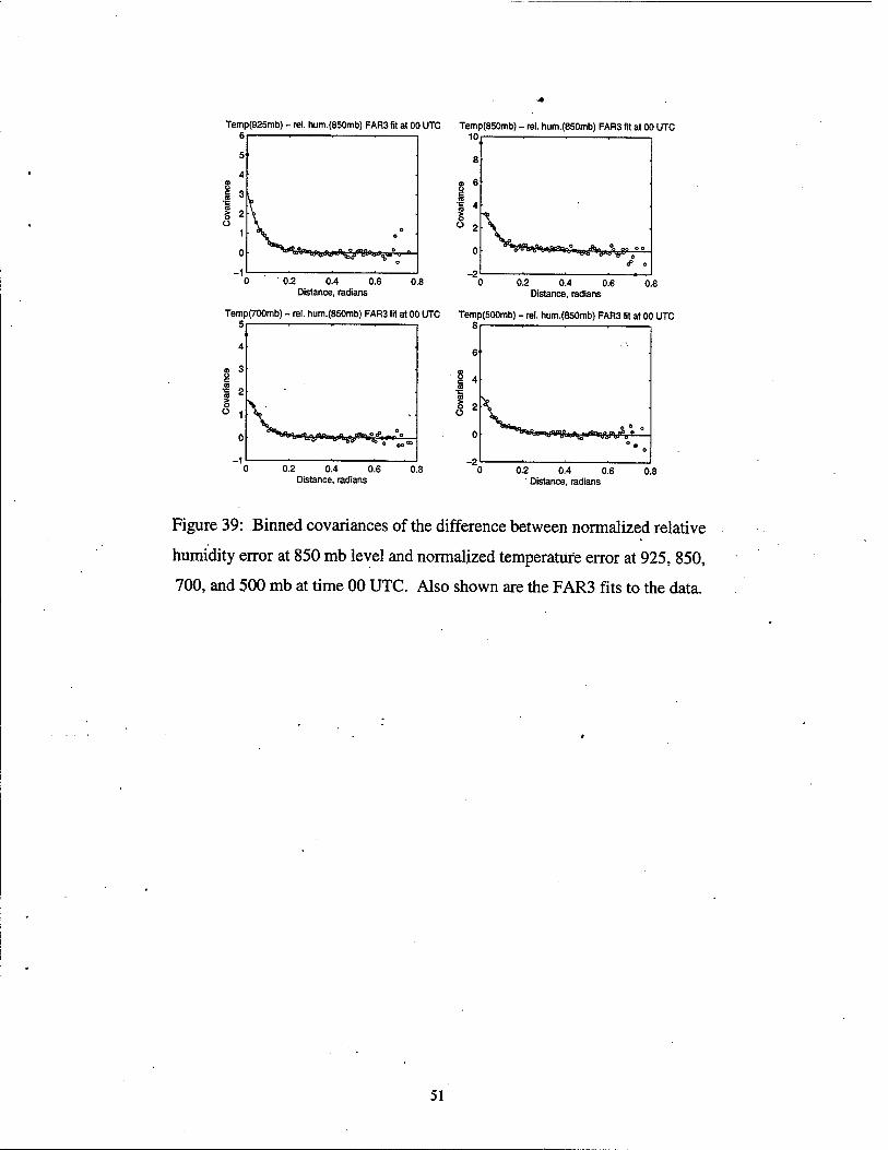
illustrate some of the data involved, Figure 39 shows the binned covariance data for four
different cases. These are the covariances between relative humidity error at 850 mb and
temperature error at 925, 850, 700, and 500 mb. Some of the nuances of the third order
• autoregressive function are shown, as well. The 925 mb temperature data illustrates that
the function may have a very sharp transition from zero slope at the origin to a rapid
decrease. Some subtle "waviness" is shown for the 850 mb and 500 mb temperature
data.
When the intercept values obtained from fitting all differences are used in Eq. (6) the
correlation matrix for the relative humidity and temperature errors are then available.
The results were computed for both the SAR2 and FAR3 fits. -
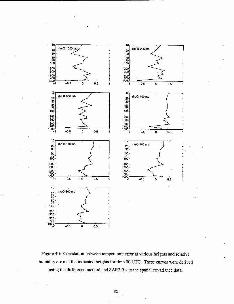
The results obtained from the SAR2 fits at times 00 UTC and 12 UTC are shown in
Figures 40 and 41, respectively. Figure 40 should be compared with Figure 35, and
Figure 41 with Figure 36. Depending on the level, some graphs compare rather well,
while there are significant differences in other cases. There are no "out of bounds" points
resulting from the difference method, in contrast to the two resulting from SAR2 fits
using the direct method. The difference method tends to show a significant drift toward
positive correlations at the higher temperature levels (generally above 200 mb, but lower
in a few cases) that are not shown in the direct method calculations. No explanation for
this has come to mind, although the investigator would urge skepticism concerning the
reality of such results.
12
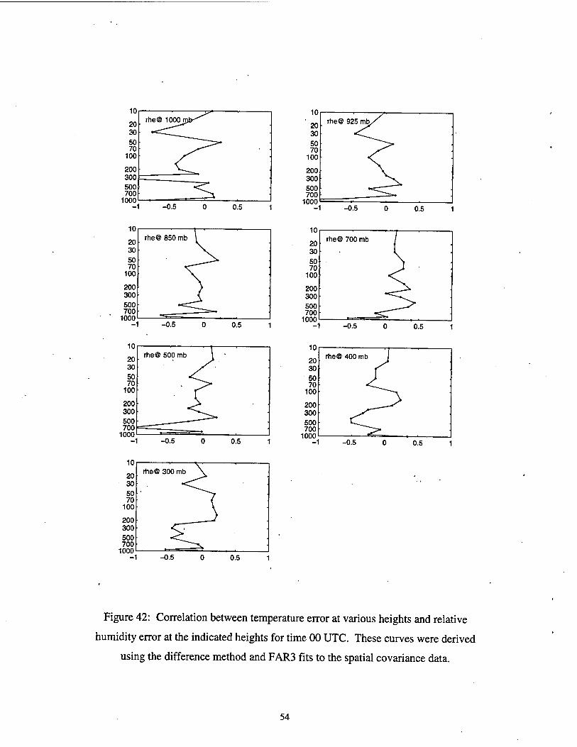
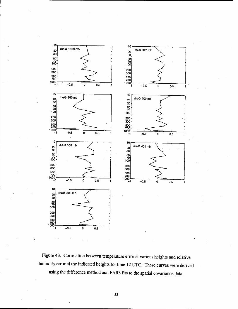
For the FAR3 fits the plots for 00 UTC and 12 UTC are shown in Figures 42 and 43,
and should be compared with Figures 37 and 38. In contrast to the SAR2 fits, the "out of
bounds" points with FAR3 are now obtained using the difference method rather than the
direct method. The curves in Figures 42 and 43 tend to show greater variation over the
temperature levels than those of Figures 37 and 38. The strong negative correlation
between relative humidity errors and temperature errors at the same level are somewhat
suppressed, and in some cases the correlation is positive.
As a general rule, the correlation curves shown in Figures 37 and 38 are the most
pleasing in the sense that they tend not to show large correlations between relative
humidity errors and temperature errors at widely differing levels. A notable exception to
this is the significant (varying positive and negative) correlation between relative
humidity error at 1000 mb and temperature error at upper levels at time 00 UTC. The
correlations are smaller at 12 UTC.
5. Summary and conclusions
This study has attempted to determine some of the properties of the spatial
covariance and vertical correlation of temperature and relative humidity prediction errors,
and their vertical cross-correlation. Use of different spatial approximations has led to
consistent results in some respects such as the variance of prediction errors and
correlation distances for both temperature and relative humidity. The attempt to
approximate the vertical correlation functions with an isotropic function on a transformed
domain led to somewhat inconsistent results when comparing those based on spatial fits
with the SAR2 function with those based on FAR3 spatial fits. Although neither of the
two approximations gave entirely satisfactory results, the SAR2 fits had the fewest real
serious problems, such as "correlation" values between levels that are greater than one in
value.
• In attempting to fit the cross-correlation, the more pleasing results were obtained by
fitting the spatial cross-covariance data directly, even though the difference method is
based entirely on fitting spatial covariance functions (of differences) and might seem to
pose less problem of an appropriate fitting function. With the direct method the
13
additional flexibility of the FAR3 function leads to better vertical cross-correlation curves
between the two variables at different levels.
Fitting the normalized difference of the two variables in the spatial domain using
SAR2 fits yields somewhat more pleasing results for the vertical cross-correlation that
that using the FAR3 fits. There is, however, a disconcerting increase in the correlation
between relative humidity errors and temperature errors as a function of height of the
temperature errors for the results from the SAR2 fits. In the case of the difference
scheme there are no "bad points" such as were noted in Figures 35 and 36 using the
SAR2 fits directly on the spatial cross-covariance.
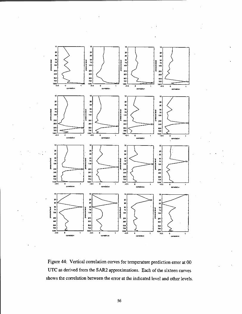
In two final figures, it is noted that the vertical correlation of temperature prediction
errors and of temperature observation errors may not be isotropic in any transformed
region. That is, for certain levels the negative lobe below the given level may not be
matched by a negative lobe at upper levels. See Figure 44 for the sixteen plots of
correlation of temperature prediction errors at 00 UTC derived from SAR2 at a given
level with those at other levels, and note especially the curves for 300 and 70 mb, and to a
lesser extent, 200 mb. Further it can be noted that the curves are different at different
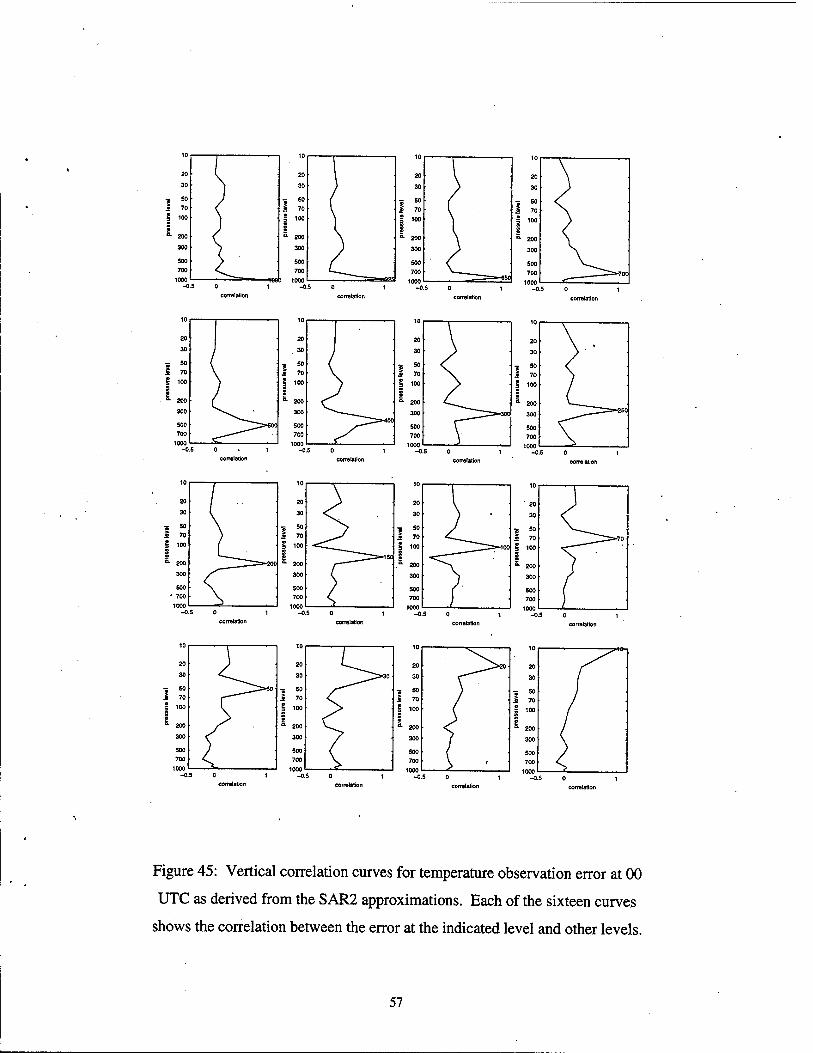
heights, indicating inhomogeneity, at least to some extent. The corresponding curves for
the associated temperature observation errors are shown in Figure 45 and exhibit some of
the same behavior. Whether such vertical correlation functions can be modeled using
positive definite functions that have the right properties is not known to the investigator.
As a matter of interest, it is noted that the empirical vertical correlation matrix for the
temperature prediction errors shown in Figure 44 is not positive definite, although that for
the temperature observation errors shown in Figure 45 is.
14
Binned temperature innovations, 850mb at 00 UTC Binned temperature innovations, 700mb at 00 UTC 2, . , , 1 2r
0.2 0.4 0.6 Distance, radians
-0.5 0.2 0.4 0.6 0.8
Distance, radians
Binned temperature innovations, 500mb at 00 UTC Binned temperature innovations, 400mb at 00 UTC 2r
0.2 0.4 0.6 Distance, radians
0.2 0.4 0.6 Distance, radians
Figure 1: Binned temperature innovations for 00 UTC
at 850,700, 500, and 400 mb levels.
Station pairs, 850mb temperature at.00 UTC Station pairs, 700mb temperature at 00 UTC
0.0 0.1 0.2 0.3 0.4 0.5 0.6 0.7 Bin distance, radians
Station pairs, 500mb temperature at 00 UTC
0.0 0.1 0.2 0.3 0.4 0.5 0.6 0.7 Bin distance, radians
0.0 0.1 0.2 0.3 0.4 0.5 0.6 0.7 Bin distance, radians
Station pairs, 400mb temperature at 00 UTC
0.0 0.1 0.2 0.3 0.4 0.5 0.6 0.7 Bin distance, radians
Figure 2: Bar chart showing number of terms in each
bin for Figure 1.
15
Binned rel 0.05
humidity innovations, 850 mb level at 00 UTC Binned rel. humidity innovations, 700 mb level at 00 UTC 0.05 r
0.2 0.4 0.6 Distance, radians
0.2 0.4 0.6 Distance, radians
Binned rel 0.05
humidity innovations, 500 mb level at 00 UTC Binned rel. humidity innovations, 400 mb level at 00 UTC 0.05 r
0.2 0.4 0.6 Distance, radians
0.2 0.4 0.6 Distance, radians
Figure 3: Binned relative humidity innovations for 00 UTC
at 850,700, 500, and 400 mb levels.
Station pairs, 850 relative humidity at 00 UTC Station pairs, 700 relative humidity at 00 UTC
0.0 0.1 0.2 0.3 0.4 0.5 0.6 0.7 Bin distance, radians
Station pairs, 500 relative humidity at 00 UTC
0.0 0.1 02 0.3 0.4 0.5 0.6 0.7 Bin distance, radians
0.0 0.1 0.2 0.3 0.4 0.5 0.6 0.7 Bin distance, radians
Station pairs, 400 relative humidity at 00 UTC
0.0 0.1 0.2 0.3 0.4 0.5 0.6 0.7 Bin distance, radians
Figure 4: Bar chart showing number of terms in each
bin for Figure 3.
16
Temperature prediction error estimates 00 UTC 101 1 -
X) E
I o 2 3
20
30
SO-
70-
100
Q- 200
300
500
700
1000 L- 0.5
Temperature prediction error estimates 00 UTC 10i . 1 1—
xi E
t a 3 ID in £ Q.
20-
30
50
70
100
200
300
500
700
1 1.5 2 Standard deviation, °C
10001— 0.5 1 1.5 2
Standard deviation, °C
Temperature prediction error estimates 12 UTC Temperature prediction error estimates 12 UTC IU *■£
20 "
30 ft
o S2W1
ja 50 > S2W2 . fc j0
70 "V . ■> • S2W3 a <D 100 - 3 D S2W4 0) \ \- CO 0) N \ a. 200 ^^-* ■
300 fry ■
500 - 700
■innn
■
0.5 1 1.5 2 Standard deviation, °C
2.5
XI E
1
a a.
IU
20
30 /£•" O S22W1
■
50 • *7^ ."'jt* « S22W2 -
70 ■
■«Sj . S22W3 ■
100 N \ D F3W1
200 ■
300
s» •
500
700
nnn
V.T ■
0.5 1 1.5 2 Standard deviation, °C
2.5
Figure 5: Plots of standard deviations of temperature prediction errors inferred
from spatial covariance fits 1-8 in Table 1 for times 00 and 12 UTC.
17
Relative humidity prediction error estimates 00 UTC 10. 1 . . .
20
30
| 50
Ö* 70
8
tt>
100
200
300 h
500
700
1000 0.05 0.1 0.15 0.2 0.25
Standard deviation 0.3
Relative humidity prediction error estimates 00 UTC 10
20
30
a 50 fc 70 > a
100 3 V) 0} <D
a. 200
300
500
700 h
1000
o S22W1
> S22W2 •
' • S22W3 "
a F3W1
■ ■
■ ■
-** ^~&r^~~ -»»^t**"^ ** —**^
0.05 0.1 0.15 0.2 0.25 Standard deviation
0.3
Relative humidity prediction error estimates 12 UTC 10i . . . .
20
30
50
70
100
1000 0.05 0.1 0.15 0.2 0.25
Standard deviation 0.3
Relative humidity prediction error estimates 12 UTC 10i . , , ■ ,
20
30
50
70
100
200
300
500
700
1000 0.05 0.1 0.15 0.2 0.25 0.3
Standard deviation
Figure 6: Plots of standard deviations of relative humidity prediction errors
inferred from spatial covariance fits 1-8 in Table 1 for times 00 and 12 UTC.
18
10 Temperature errors 00 UTC from SAR2
£
1
20
30-
50-
70
100-
a. 200-
300-
500-
700-
10001— 0.5 1 1.5 2
Standard deviation, °C
£ a.
10 Temperature errors 00 UTC from FAR3
20 r
30
| 50
ä" 70 a S 3
100-
200-
300-
500
700
1000 ■— 0.5 1 1.5 2
Standard deviation, °C
Temperature errors 12 UTC from SAR2
.a E
1
QL
1000 0.5
J2 E
1
2 Q.
1 1.5 2 Standard deviation, °C
10
20
30
50
70
100
200-
300
500
700
1000
Temperature errors 12 UTC from.FAR3
1 2 Standard deviation, °C
Figure 7: Temperature observation and prediction errors inferred from spatial covariance fits by SAR2 and FAR3 in for times 00 and 12 UTC.
19
10 Relative humidity errors 00 UTC from SAR2
20
30
n 50 fc 'S 70 > m
100 3 </> <n (D
0. 200
300
500
700
1000
20
30
■
E 50
prediction error • - A) observation error 5
0
CO
100
0.05 0.1 0.15 0.2 Standard deviation
0.25
10 Relative humidity errors 00 UTC from FAR3
0- 200
300
500
700
1000
predtetion error
observation error
0.05 0.1 0.15 0.2 Standard deviation
0.25
10
20
30
I 50
■5 70 £ 8 3
Relative humidity errors 12 UTC from SAR2
a.
100
200
300
500
700 r
1000
prediction error
observation error
0.05 0.1 0.15 0.2 Standard deviation
0.25
a ■ a.
10 Relative humidity errors 1.2 UTC from FAR3
20r
30
50
70
100 r
200
300-
500
700
1000
D pre<Sction error
O observation error
0.05 0.1 0.15 0.2 Standard deviation
0.25
Figure 8: Relative humidity observation and prediction errors inferred from
spatial covariance by SAR2 and FAR3 fits for times 00 and 12 UTC.
20
Temperature prediction error from SAR2 at 00 UTC Temperature prediction error from FAR3 at 00 UTC 40i ■ 1 ■ 1 40r
30
20
S 10r c a w ' 0 Q.
o ra-10
-20-
-30-
-40
ft-
-1 -0.5 0 0.5 correlation
-0.5 0 0.5 correlation
Temperature prediction error from SAR2 at 12 UTC Temperature prediction error from FAR3 at 12 UTC HU
30 i » *
>i 20 »• •
••• •
K" 8 10 to ^i* . (O *' "^rr.. "° 0 "• * ° —
0. ** • "*%»1^ * Ol o ra-10 <<"
> **
-20
t
•« • > a
-30 t
An
«tu "" "' "■" —i I
30 • a 0 O
20 y p • 0 .
8 10
a • • •
fto° • c J^F- % CO • • *^**" ,„ 2. o a. • • .<£& '" D> ^tv-s. o ?72i 8
"5-10
-20
* • 4 *
V • •
• ° 0
•• ■
-30 ■ •• •
ATI
-0.5 0 0.5 correlation
-1 -0.5 0 0.5 correlation
Figure 9: Temperature prediction error correlations in the transformed
coordinate system derived from SAR2 and FAR3 fits at 00 and 12 UTC.
21
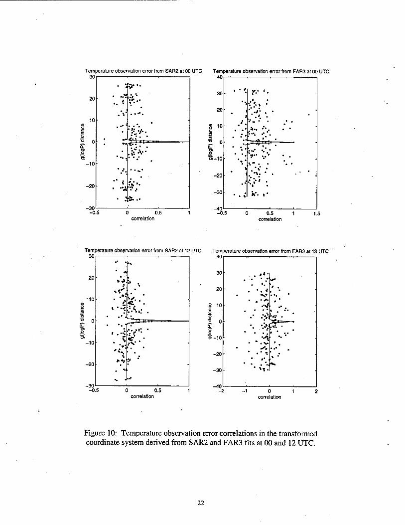
Temperature observation error from SAR2 at 00 UTC Temperature observation error from FAR3 at 00 UTC 30
20
10
D. o> o
-10
-20-
-30 -0.5
1. •'
?S" =t£:
ft''
•4«*** *
0 0.5 correlation
40
30
20
8 10 c eg w
2. o 0. o "5-10-
-20-
-30
-40 -0.5
•■••::•» •
• . • . .• ft». •*. • ■•
• .:•••. ••■.
• --v- ...*• • • v..-. ...
0 0.5 correlation
1.5
Temperature observation error from SAR2 at 12 UTC Temperature observation error from FAR3 at 12 UTC 30| > 1 1. 40r
20-
•10-
o. o
-10
-20
-30 -0.5
•• • ••* • * • ' V4 '* . / •
*'.' • •: . • •
< • • '•• •«. •
• • * a
* "• 1
• •
a»
. * : ?
*»-. • * •
*v ."» * • ■
. v
•• * .*
0 0.5 correlation
30-
20-
8 10r c ffl "5
o. oi o 'S-10
-20
-30-
-40
. /<•! • ■•
#* • ••
• • * »
• ■N* • •• •
. • • * •
r • ••. ■•v • «•r*^==™™—•
• ■ • . 1 • .. • •• • •
-'. ••• » •'
' '• d -*.
-1 0 1 correlation
Figure 10: Temperature observation error correlations in the transformed coordinate system derived from SAR2 and FAR3 fits at 00 and 12 UTC.
22
Relative humidity prediction error from SAR2 at 00 UTC Relative humidity prediction error from FAR3 at 00 UTC
0 correlation
0 0.5 correlation
Relative humidity prediction error from SAR2 at 12 UTC Relative humidity prediction error from FAR3 at 12 UTC 30i ! 1 ■ 1 1 40
30-
20-
g 10- c
0- 0. o>
0 0.5 correlation
ra-10-
-20-
-30-
-40 -0.5
0 . • •.
*
* » • • * O °
0 0.5 correlation
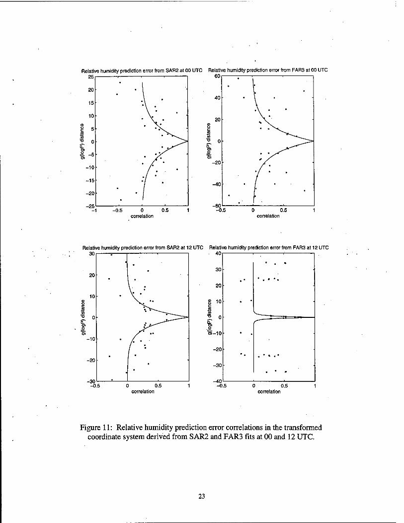
Figure 11: Relative humidity prediction error correlations in the transformed coordinate system derived from SAR2 and FAR3 fits at 00 and 12 UTC.
23
Relative humidity observation error from SAR2 at 10
00 UTC Relative humidity observation error from FAR3 at 00 UTC 10r
0 0.5 correlation
-0-5 0 0.5 correlation
Relative humidity observation error from SAR2 at 20
15-
10
* s o 3
c- a w Z 0 0. O) o oi -5 ■
-10
-15
-20 -0.5
• ••
as ■
• •• *
*
—■—
i—
i—
1—
i—
i
i
12 UTC Relative humidity observation error from FAR3 at 12 UTC 15r
0 0.5 correlation
-0.5 0 0.5 correlation
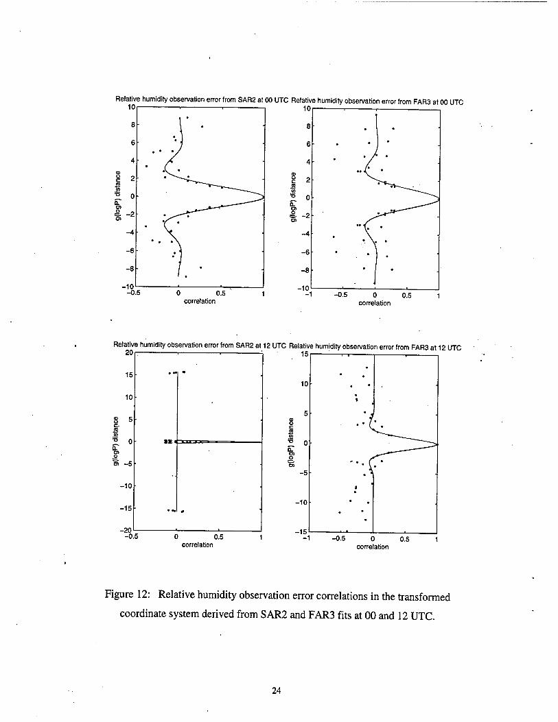
Figure 12: Relative humidity observation error correlations in the transformed
coordinate system derived from SAR2 and FAR3 fits at 00 and 12 UTC.
24
temperature prediction error from SAR2 at 00 UTC temperature prediction error from FAR3 at 00 UTC 10r > ' 1 1 10r
20 g(logP)
20 g(iogP)
tern 10
20
perature prediction error from SAR2 at 12 UTC temperature prediction error from PAR3 at 12 UTC
20
30 / 30
50 / 50
I 70 / 1 70
Pre
sure
,
O
O
| 100 <0 CD
O-
200 200 / *
300 / 300
500 / 500
700 ■ ^X 700
0 10 .20 30 40 0 10 20 30 40 g(iogP) g(logP)
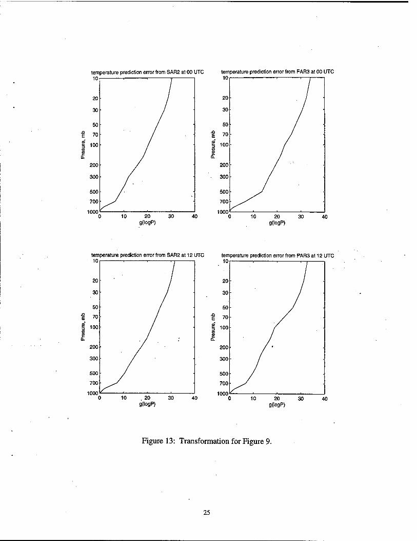
Figure 13: Transformation for Figure 9.
25
temperature observation error from SAR2 at 00 UTC temperature observation error from FAR3 at 00 UTC 10, 1 . 1 1 10
10 20 g(iogP)
20 g(iogP)
temperature observation error from SAR2 at 12 UTC temperature observation error from FAR3 at 12 UTC 10r ■ ' 1—I 10
10 20 g(iogP)
20 g(iogP)
Figure 14: Transformation for Figure 10.
26
relative humidity prediction error from SAR2 at 00 UTC relative humidity prediction error from FAR3 at 00 UTC
300
.o E
1000 10 20
g(iogP) 20 40
g(iogP)
relative humidity prediction error from SAR2 at 12 UTC relative humidity prediction error from FAR3 at 12 UTC
300-
J3 E
500-
Q.
700-
1000 10 20
g(iogP)
£1 E
£ o.
1000 20
gdogP)
Figure 15: Transformation for Figure 11.
27
relative humidity observation error from SAR2 at 00 UTC relative humidity observation error from FAR3 at 00 UTC
300
n B
500- <D
1000
700-
1000 02468 10 02468 10
g(logP) g(logP)
relative humidity observation error from SAR2 at 12 UTC relative humidity observation error from FAR3 at 12 UTC
300
E
500 m a.
5 .10 g(iogP)
700
1000 5 10
g(iogP)
Figure 16: Transformation for Figure 12.
28
Temperature prediction error at 00 UTC from SAR2
£
2 a.
IU T—' ' ——■» -• »—T— ; /
20 o ' s an ■
/ 30 "v- / o« o
■
50 0 I • JBO ■
70 ^< -v - ~' . ( / •
100 - ( > -*K \o
200 1 o '^TsCOO-
J. ..«-.\ tro' 300 0 •
500 G o \V ■ .M00-
700 "■-" °' ' | '-^6 o ■
000 . ■ °ft"*7I~TT
Temperature prediction error at 00 UTC from SAR2 10r
20
30
50
70
100
2 D.
-0.5 0 0.5 Correlation
200
300 r
500
700
1000
\ •>. "■.
i
0 * "n
* O Jft30 .
■Y ~ "" ""
*>. s
^ ■ ff" ö TV
°"*' O /J* '.'«400
•t^j^o
" -i° ♦., • "~—s»» -0.5 0 0.5
Correlation
E
s o s 3 to
' (O 2 0-
Temperature prediction error at 00 UTC from SAR2 10
20
30
50
■5 70
100-
200
3001-
500
700
1000
■T r*»^ 1 1 ,
** "* \ N *i *20 ■
V -
> A»- " S / V .-
■,** v > * *o- L_JP_ _
/ ~' — - • / o fcioo-
-•—< «;• ♦
o'bv » Oi
x ■'. D \>6 O
'' ■■• *v «r-*-"*""!?*
> Si—■ I \ 2— "i i -0.5 0 0.5
Correlation
Temperature prediction error at 00 UTC from SAR2 10
0 0.5 Correlation
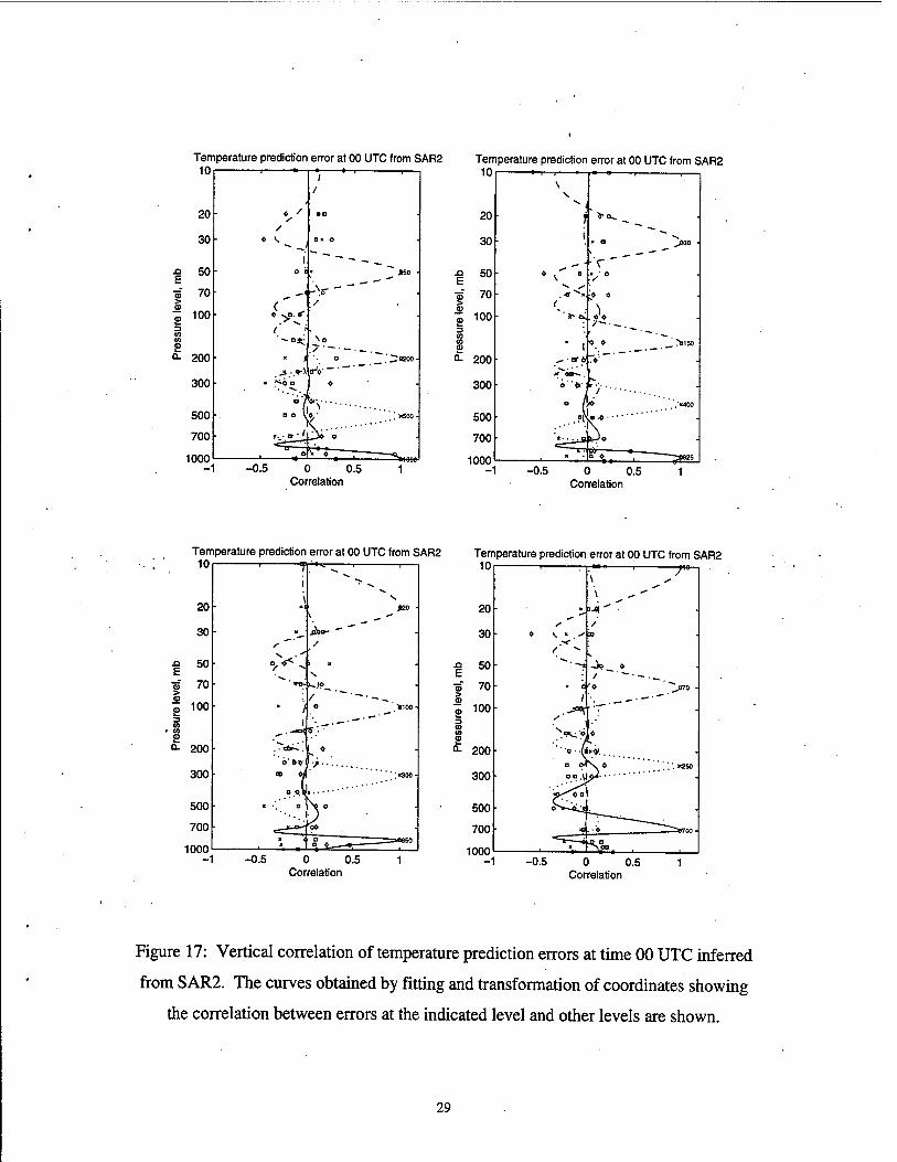
Figure 17: Vertical correlation of temperature prediction errors at time 00 UTC inferred
from S AR2. The curves obtained by fitting and transformation of coordinates showing
the correlation between errors at the indicated level and other levels are shown.
29
Temperature prediction error at 00 UTC from FAR3 10r " -
20
30
XI E
50
ö" 70 £ 2 3 CO CO
£ Q.
100
200
300 r
500
700
1000 -1
v ■ ■—
' y= « 0
/ 0 V. o > 0
i « o
^. .00
o» 0- x-
*•
\ O «3^ ■ - '.V '
» / «. • »;i
» >r*" o
.' 0 O ."»COO ■
on ■"'"
«o^ *'•■-■ — ...
OO <
0o 5> o
9 ■ g». I " ' _ :—■—-ct.
-0.5 0 0.5 Correlation
Temperature prediction error at 00 UTC from FAR3 10r
20
30
E 50
70
100
S o. 200
300 r
500
700
1000 -1
■o 1e>_ __
I •II» o »30 •
^ «. T " " o «f r0 j
*"*' 7 .qo
O " i • ^'.*1S0
o o»^0 '-•—•'""
O B O
-o a "<o'«••.. \ ••■...,
o ° i '.««» op , .0. • ■»
:—. ° I ., »'■ 7^- -0.5 0 0.5
Correlation
Temperature prediction error at 00 UTC from FAR3 10r
20
30
XI E
50-
ö" '70 •
CD
100
200
300
500
700
1000
/ 1
i» 1 1 1
- p. ! t ^20 •
■ <> V»d-
y I \ • »«
/■ \ . a -^* 4 1 o
«0 O |
I ■100 ■
- o^*' *r- ■
■ a "--**o •> . ■***■
o ' 0
■ o a« / V-"300 ■
°*. - J»
. * B " • ■ S 0 o
■ 0 ,_ o
Temperature prediction error at 00 UTC from FAR3
-0.5 0 0.5 Correlation
n E
CD
IU -i »w—|
20 » ■ •*•
\
tO'-D /
s
30 o 1^..- O ■
50
70
/• V
« . 0
-Jo / -
:o ~^JO<l •
100 D Jf* ' ►■' .
-:■>■. . 200 m
a
o BO r 300 'Oo ;«so
0
500
700
nnn
0
N CB ' m
£ •
^ ». -0.5 0 0.5
Correlation
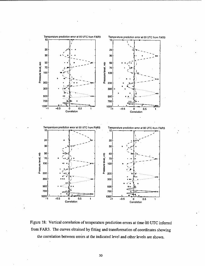
Figure 18: Vertical correlation of temperature prediction errors at time 00 UTC inferred
from FAR3. The curves obtained by fitting and transformation of coordinates showing
the correlation between errors at the indicated level and other levels are shown.
30
Temperature prediction error at 12 UTC from SAR2
£ a.
10 1 0 ■7 •-
20 o • s /
Cft ■
30 o \ ^ OK O ■
1 "" ~ — _ 50 oc t ^«50 ■
70 ■
100 /
■
*•■-; i
200 « < '■ 0 _""woo-
»,t »- '$"b
300 . ?d'' 0» ■
D
500 a o j
'•••'A'..' 700 ^ ° ■
nnn , ff^~m T- -•«101)0
-1 -0.5 0 0.5 Correlation
Temperature prediction error at 12 UTC from SAR2 10i •
£ o.
20
30
50
70
100
200
300
500
700
1000 -1
I- ^
k,
/
.06»-'. o
,0« -OB. ,y
_"S150
-0.5 0 0.5 Correlation
Temperature prediction error at 12 UTC from SAR2 Temperature prediction error at 12 UTC from SAR2
£ CO CO
£ Q.
10
i I—*■" 1 1 1
s 20
30
> O »20 -
50
70
100
/a «s
'V.'
0 * >. 34o»_
. O >100 -
200 ■'.■**■*. 0
DO < )■■■.
300 a 00 ' '': >3oo -
*.a *r<^
500 ■ •■■°.v 700 . ._-—p» nnn ,«." £v-^—; '—=^~"
-1 -0.5 0 0.5 Correlation
0 0.5 Correlation
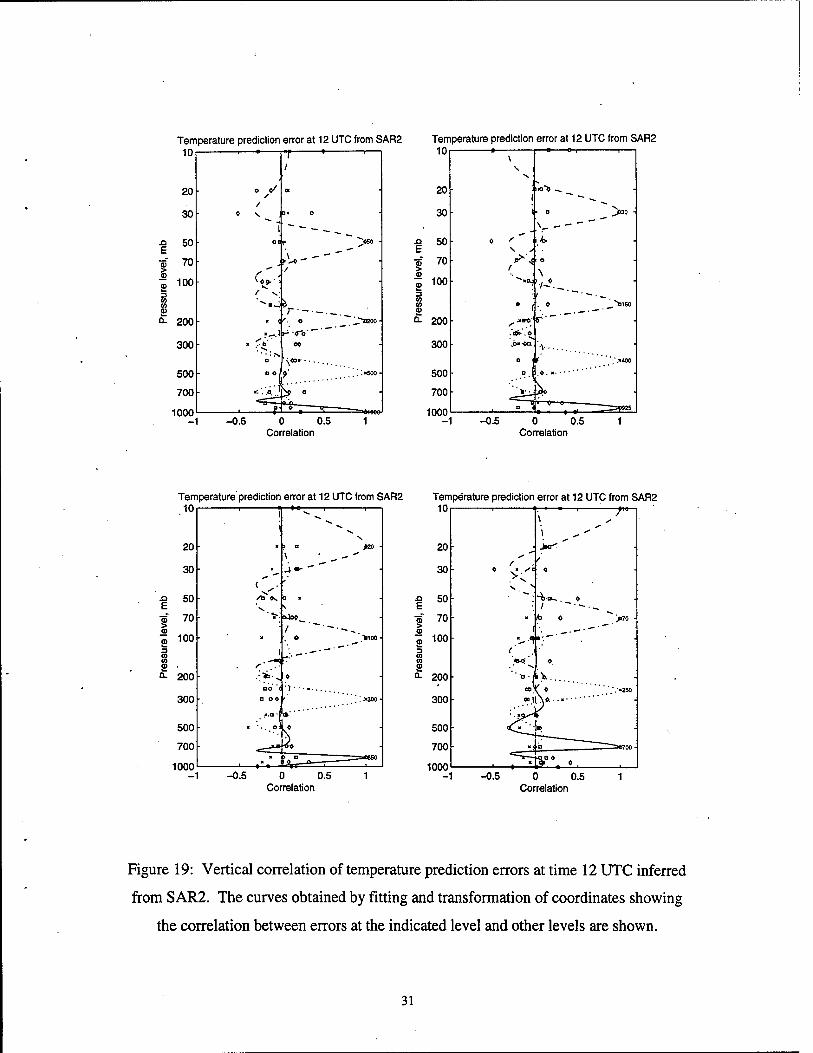
Figure 19: Vertical correlation of temperature prediction errors at time 12 UTC inferred
from S AR2. The curves obtained by fitting and transformation of coordinates showing
the correlation between errors at the indicated level and other levels are shown.
31
Temperature prediction error at 12 UTC from FAR3
I t
20 /
0 ■
30 (^a « 0 ■
50 o* _ >so ■
70
100 J
a , "-oc
OB
^ »
ö oa—{
m 200 ~«00-
■ ' '* ^M>
300 ';< ** O ■
' '• 500 o D $f. '.'.»«500 ■
700 " '•'• '■ -fo * ° •
1000 , B<=KT^~rzr-^ ~*iooo
Temperature prediction error at 12 UTC from FAR3 10
20
30
■S 50
2. 2 3 CO CO
2
-0.5 , 0 0.5 Correlation
70
100
2001-
300
500
700
1000
. , ■
\ ■* ♦ y i | 1
N. X.
"S. " »0 *. .O
■ ■ O >30 -
a p o 1 ■
""" V o y«
,- t -n-.,*
o. - *oV- •
* _~!0I50
X '■> . > 0
0"^tJ '"'«' • • . . . v ' ' ■ . .
» > ) « MOO
JL^W ♦ "n T"- o j
. -S..1 . ♦ ,~^"~==?>* -0.5 0 0.5
Correlation
. Temperature prediction error at 12 UTC from FAR3 10
Temperature prediction errorat 12 UTC. from FAR3
0 0.5 Correlation
IU ; ■ 1 f«—| S
X" ** i *"
?n M D-O-"* O r
S
30 0 ( \- e X /
X S* >
50 «y 1 Oi ()
£.
70 ( ** ° ^".'JffO ■
100 ? 0
■ '<K U,
200 " " l£o~ ■ 'j\ " • ..250
300 0 y ...'•■"" a^U«
500 o ^—~^*L
700 - *0 a " r^tmn.
nnn , "ft 3 ♦• . -1 -0.5 0 0.5
Correlation
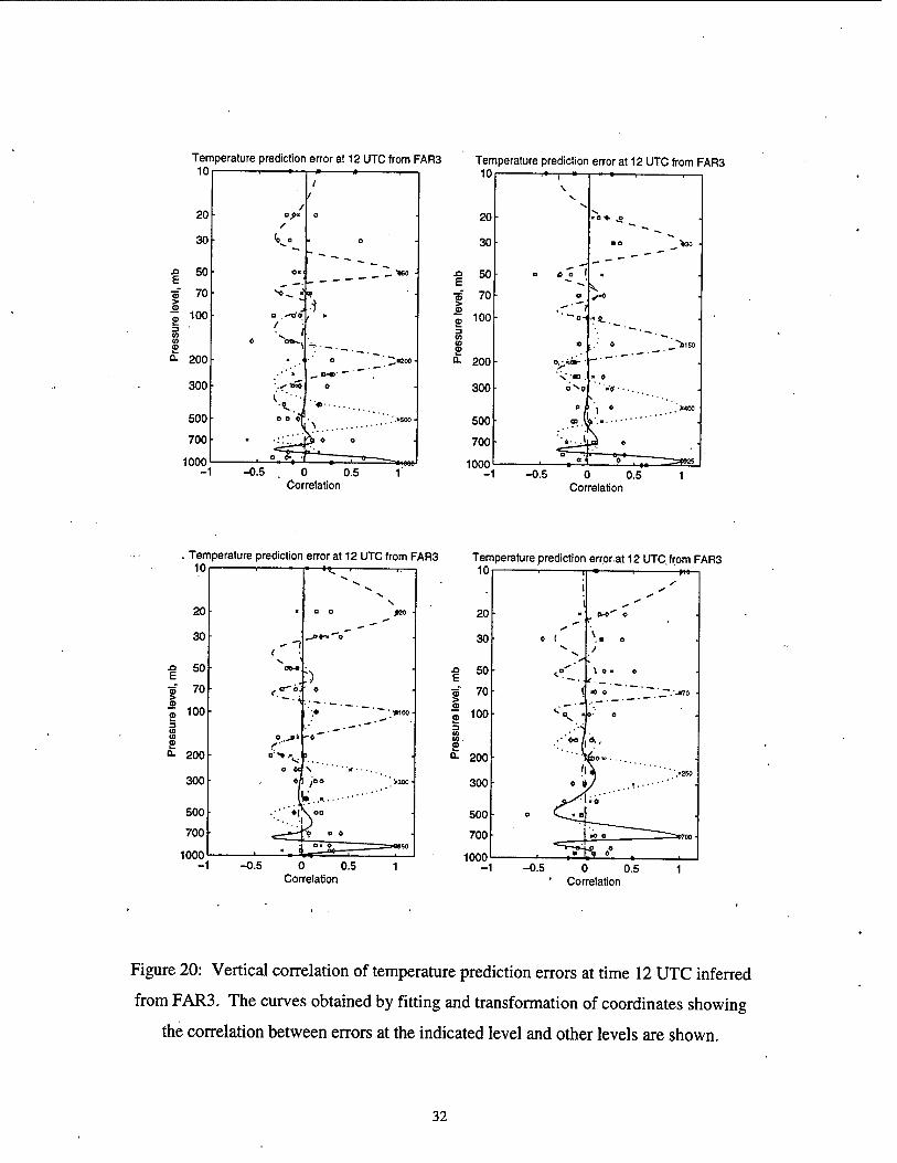
Figure 20: Vertical correlation of temperature prediction errors at time 12 UTC inferred
from FAR3. The curves obtained by fitting and transformation of coordinates showing
the correlation between errors at the indicated level and other levels are shown.
32
Temperature observation error at 00 UTC from SAR2 Temperature observation error at 00 UTC from SAR2
0 0.5 Correlation
10
20
30
•o 50-
ö" 70- > CD
m 100 r
2 Q. 200-
300
500
700
1000 -1 -0.5
■£. -^»0
1 oo
. _.'—mso
0 0.5 Correlation
Temperature observation error at 00 UTC from SAR2 Temperature observation error at 00 UTC from SAR2 10| 1 T" »-r- 1—i 10
J3 E
t m
2 (O (0
2 0.
20
30
50
70
100
200
300
500
700
1000
r- •—i 1 1
^ N. **
X
■
«O >20 -
■ * _ c D »
■
oc » «
D 0 »
■
* D O
»> O
• <x OX
. ^« 1 »
-0.5 0 0.5 Correlation
20
30
| 50-
•5 70 <D g 1001- CO CO
2 o- 200
300
500
700
1000
■
—■ 1 <H6—1
s
s it D <r
' o .* *
• 0 -a o^
*>- ■
■ D •
o to
• < <* D
O D.'D.-. ■.-.-—■ ..-.«250
■ < O O ■
« rfr^ o
■ * *>-^^
■ « '» ——*700-
-0.5 0 0.5 1 Correlation
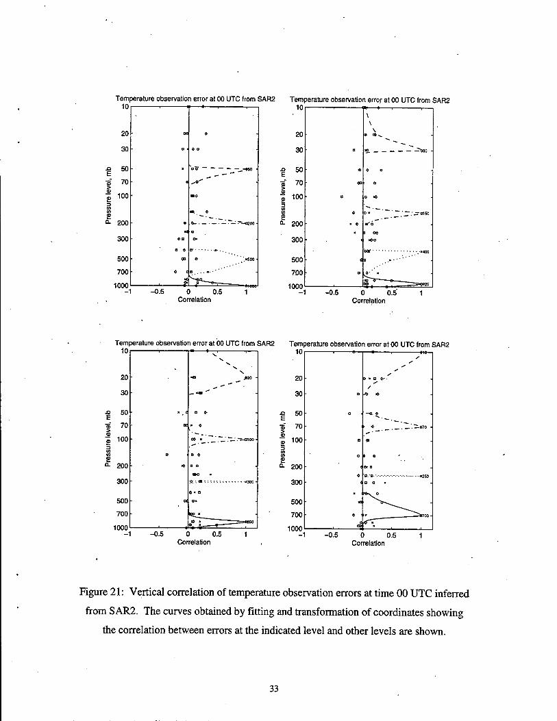
Figure 21: Vertical correlation of temperature observation errors at time 00 UTC inferred
from SAR2. The curves obtained by fitting and transformation of coordinates showing
the correlation between errors at the indicated level and other levels are shown.
33
Temperature observation error at 00 UTC from FAR3 Temperature observation error at 00 UTC from FAR3 10
20
30
50-
70
100
<D
£ 200
300
.500
700
-0.5 0 0.5 Correlation
1000 -1
—• v*— r— \ \
• 0
I
/ . o
• O 0 MO
■ 0 c »o
—*o- * *" o - O O O
■ O*- .. o . * 0
< o ö ;.«400
• . R ^J> o
♦ .\?r>^ -0.5 0 0.5
Correlation
Temperature observation error at 00 UTC from FAR3 101 ■ •^ •»!-
20-
30-
50-
70
100r
£ °- 200
300-
500-
700 ■
1000
/ I «o
> o
\ JKO
• «■• JJ .•—.-.=■■• ~ o
-0.5 0 0.5 Correlation
Temperature observation error at 00 UTC from FAR3' 10r
20
30
50
70
100
Q- 200-
300-
500
700
1000 -1
——e ■ i »io /
s s
s
"
0 • oo 1
- oo ■ o
• o *.'_!". 'aZT. 0=~- •-=-■•-—. -«70 ■
' a MO
a o ■ o
■ O 1 0
o
■ OO H «
O m 0 o
• a> a
- J -0.5 0 0.5
Correlation
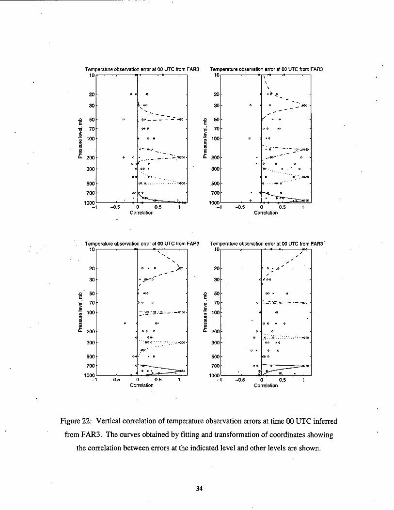
Figure 22: Vertical correlation of temperature observation errors at time 00 UTC inferred
from FAR3. The curves obtained by fitting and transformation of coordinates showing
the correlation between errors at the indicated level and other levels are shown.
34
Temperature observation error at 12 UTC from SAR2 Temperature observation error at 12 UTC from SAR2 10 1 » « 1U
\ \
20 xc a ♦ • 20 \
»0 0^
30 D 0 0 30 D
| 50 ■ 0 n 50 * < o 0
ress
ure
leve
l,
o
o
•>
D
a
* o
0
Pre
ssur
e le
vel,
ro
-»
O
O
-J
o
o
o
> 0 D
O 0 * 0
* «t o Q- 200 * — a-" ' X >o 0
300 * • "■."
300 0 ■o •»
DC» 0 ' ■ - . o ft Q >400
500 • O ' .»500 • 500 • , ' ■ *-•■•'
700 ♦ 700 0 oo' *
•* «0
1000 * i 0
1000 1 -0.5 0 0.5 1 1 -0.5 0 0.5 1
Co relation Correlation
Temperature, observation error at 12 UTC from SAR2 Temperature observation error at 12 UTC from SAR2
0 0.5 Correlation
0 0.5 Correlation
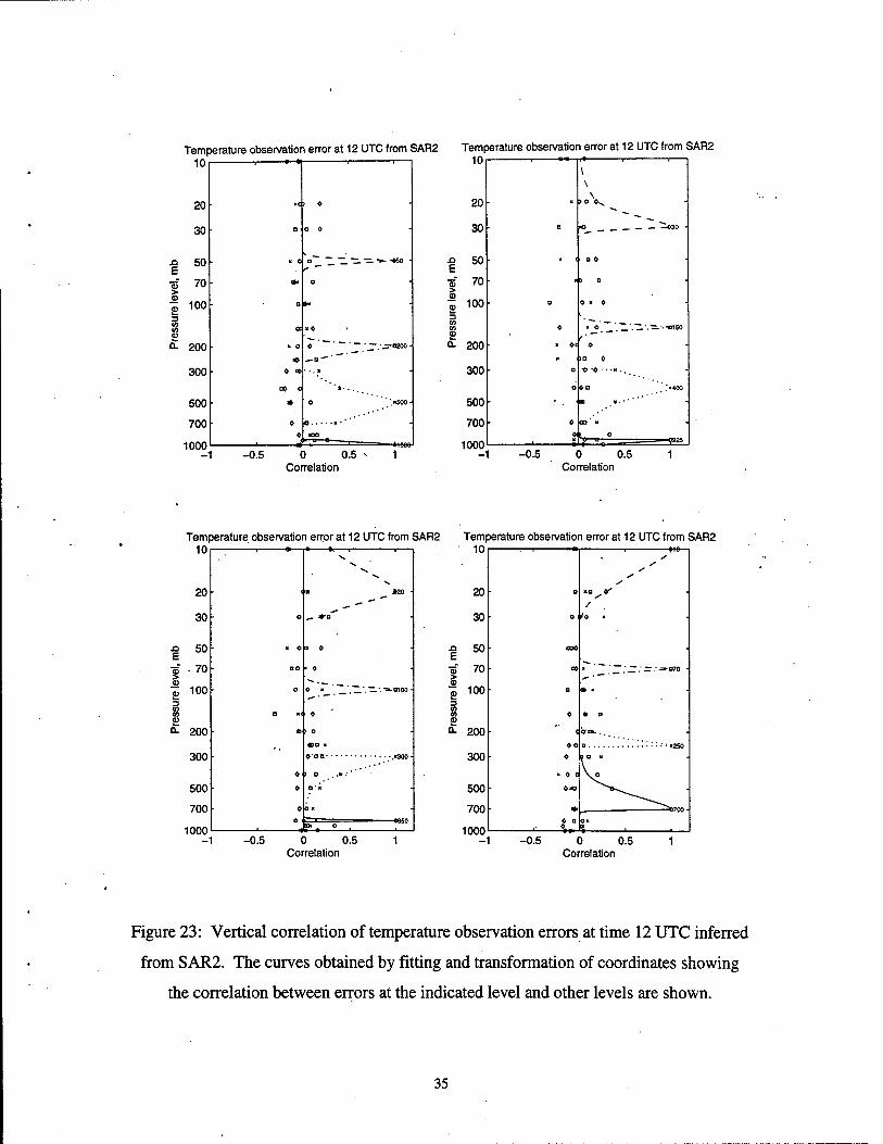
Figure 23: Vertical correlation of temperature observation errors at time 12 UTC inferred
from S AR2. The curves obtained by fitting and transformation of coordinates showing
the correlation between errors at the indicated level and other levels are shown.
35
Temperature observation error at 12 UTC from FAR3 Temperature observation error at 12 UTC from FAR3 10
20 o «00
30 o« n a
e le
vel,
mb
o
-«J
en
o
o
o
■
0
♦
o ~ — >50 ■
io *-0*"
/ t 0
Z3 CD CO
£ 200
1
K
oca
» o 0
0 _ . "_T". 'S~- "-T". '-=■* -C200 ■
300 ■ DO 0
0 oo . 500 a .
700
1000
a> o
en 1 ■—
:
i^ ' «IUUU -1 -0.5 0 0.5
Correlation
10
20
30
■| 50
■5 70 CD
m 100
£ 200
300
500
700
1000 -1
_"*30
O _'.~ \ —-. — ■••«150
-0.5 0 0.5 1 Correlation
Temperature observation error at '12 UTC from FAR3 Temperature observation error at 12 UTC from FAR3 101 1-» ■ I »
20
30
£> 50 b
70 > a <l> 100 3 CO en 0) 0. 200
300
500
700
1000
• O O
DO '
i o O
>20 ■
^♦'
-1
-*?moo ■
-0.5 0 0.5 1 Correlation
1U
20 o
• 1 fn—
*-•
1
30 . O 0
e le
vel,
mb
o
^
01
o
o o
0 ■ <
0 ■
• o »
0 _ ^070 ■
Pre
ssur
O
O
0 ■
0 « 0
J <0
o
O DO
300 ■ a o ♦
500
700
0 o
«a
. —.*'
0
^ L mnn
o ■ ■o .
-1 -0.5 0 0.5 1 Correlation
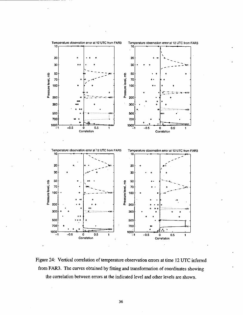
Figure 24: Vertical correlation of temperature observation errors at time 12 UTC inferred
from FAR3. The curves obtained by fitting and transformation of coordinates showing
the correlation between errors at the indicated level and other levels are shown.
36
Relative humidity prediction error at 00 UTC from SAR2 Relative humidity prediction error at 00 UTC from SAR2 10, . . . 1—, I0r
-0.5 0 0.5 1 Correlation
-0.5 0 0.5 1 Correlation
Relative humidity prediction error at 00 UTC from SAR2 Relative humidity prediction error at 00 UTC from SAR2 10| 1 1 1 : 1 1 10r
-0.5 0 0.5 1 Correlation
-0.5 0 0.5 Correlation
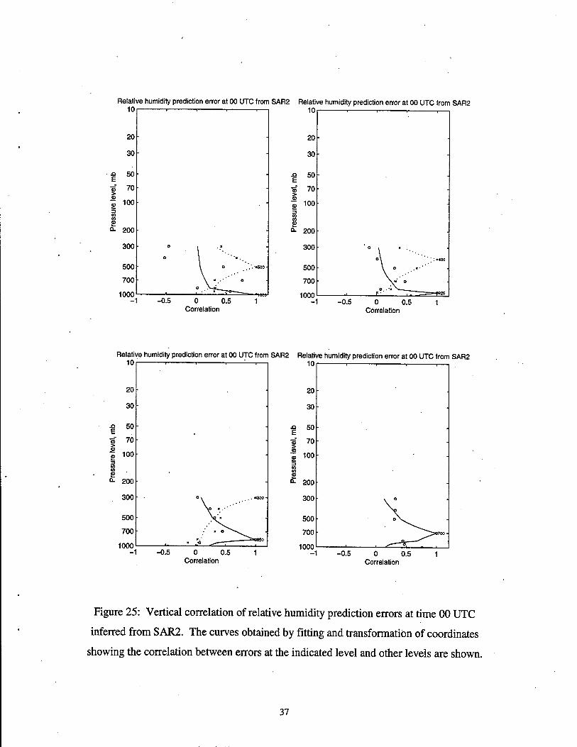
Figure 25: Vertical correlation of relative humidity prediction errors at time 00 UTC
inferred from SAR2. The curves obtained by fitting and transformation of coordinates
showing the correlation between errors at the indicated level and other levels are shown.
37
Relative humidity prediction error at 00 UTC from FAR3 Relative humidity prediction error at 00 UTC from FAR3 10i ■ . . .—i 10
-0.5 0 0.5 1 Correlation
-0.5 0 0.5 1 Correlation
Relative humidity prediction error at 00 UTC from FAR3 Relative humidity prediction error at 00 UTC from FAR3 10i . . . .—i 10r
-0.5 0 0.5 1 Correlation
-0.5 0 0.5 1 ■ Correlation
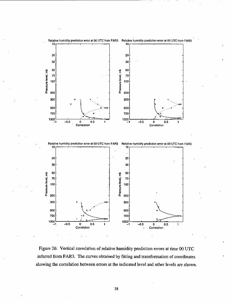
Figure 26: Vertical correlation of relative humidity prediction errors at time 00 UTC
inferred from FAR3. The curves obtained by fitting and transformation of coordinates
showing the correlation between errors at the indicated level and other levels are shown.
38
Relative humidity prediction error at 12 UTC from SAR2 Relative humidity prediction error at 12 UTC from SAR2 10. ■ . . .—i ' 10r
-0.5 0 0.5 Correlation
-0.5 0 0.5 1 Correlation
Relative humidity, prediction error at 12 UTC from SAR2 Relative humidity prediction error at 12 UTC from SAR2' 10i ■ ■ ■ .—i 10
-0.5 0 0.5 Correlation
-0.5 0 0.5 Correlation
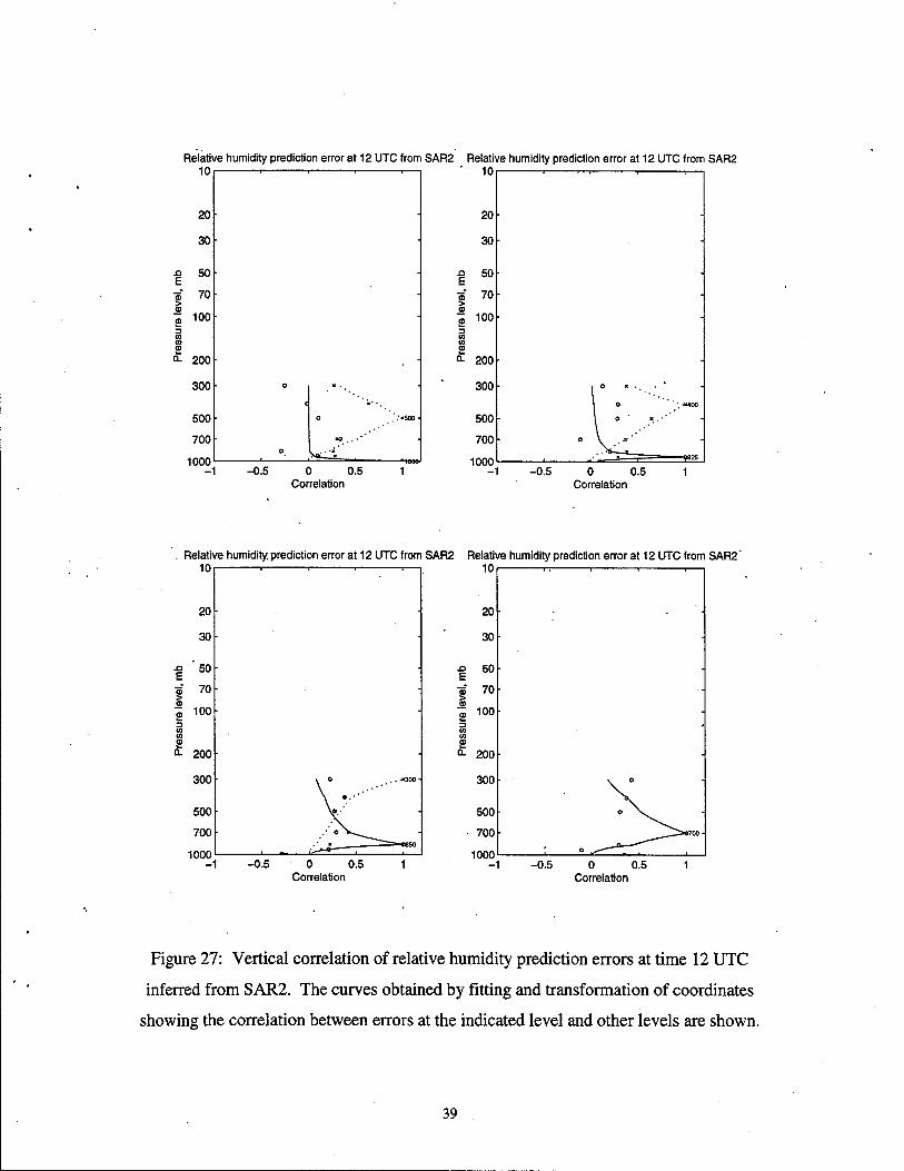
Figure 27: Vertical correlation of relative humidity prediction errors at time 12 UTC
inferred from SAR2. The curves obtained by fitting and transformation of coordinates
showing the correlation between errors at the indicated level and other levels are shown.
39
Relative humidity prediction error at 12 UTC from FAR3 Relative humidity prediction error at 12 UTC from FAR3 10, ■ , 1 r-
-0.5 0 0.5 Correlation
20
30
| 50
05 70 > o m 100
0- 200
300
500
700
1000 -1 -0.5 0 0.5 1
Correlation
Relative humidity prediction error at 12 UTC from FAR3 Relative humidity prediction error at 12 UTC from FAR3 10. 1 1 ■ 1—i 10
£ Q.
20
30
50
70
100
200
300
500
700
1000 -1 -0.5 Q 0.5 1
Correlation
ja E
> JE £ 3
20
30
50
70
100
0- 200
300
500
700
1000 -1 -0.5 0 0.5 1
Correlation
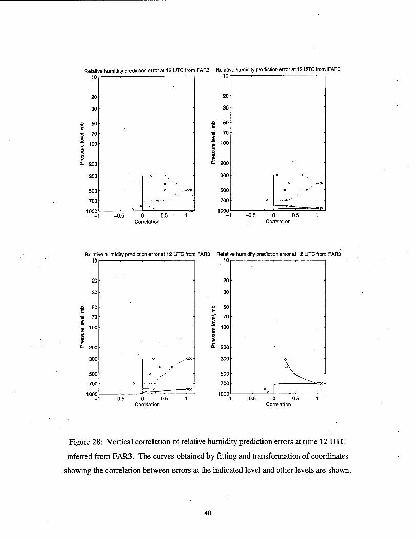
Figure 28: Vertical correlation of relative humidity prediction errors at time 12 UTC
inferred from FAR3. The curves obtained by fitting and transformation of coordinates
showing the correlation between errors at the indicated level and other levels are shown.
40
Relative humidity observation error at 00 UTC from SAR2 Relative humidity observation error at 00 UTC from SAR2 10. 1 1 1 1—i 10r
-0.5 0 0.5 Correlation
-0.5 0 0.5 1 Correlation
Relative humidity observation error at 00 UTC from SAR2 Relative humidity observation errorat 00 UTC from SAR2 10i . 1 ■ 1—i 10r
-0.5 0 0.5 Correlation
0 0.5 Correlation
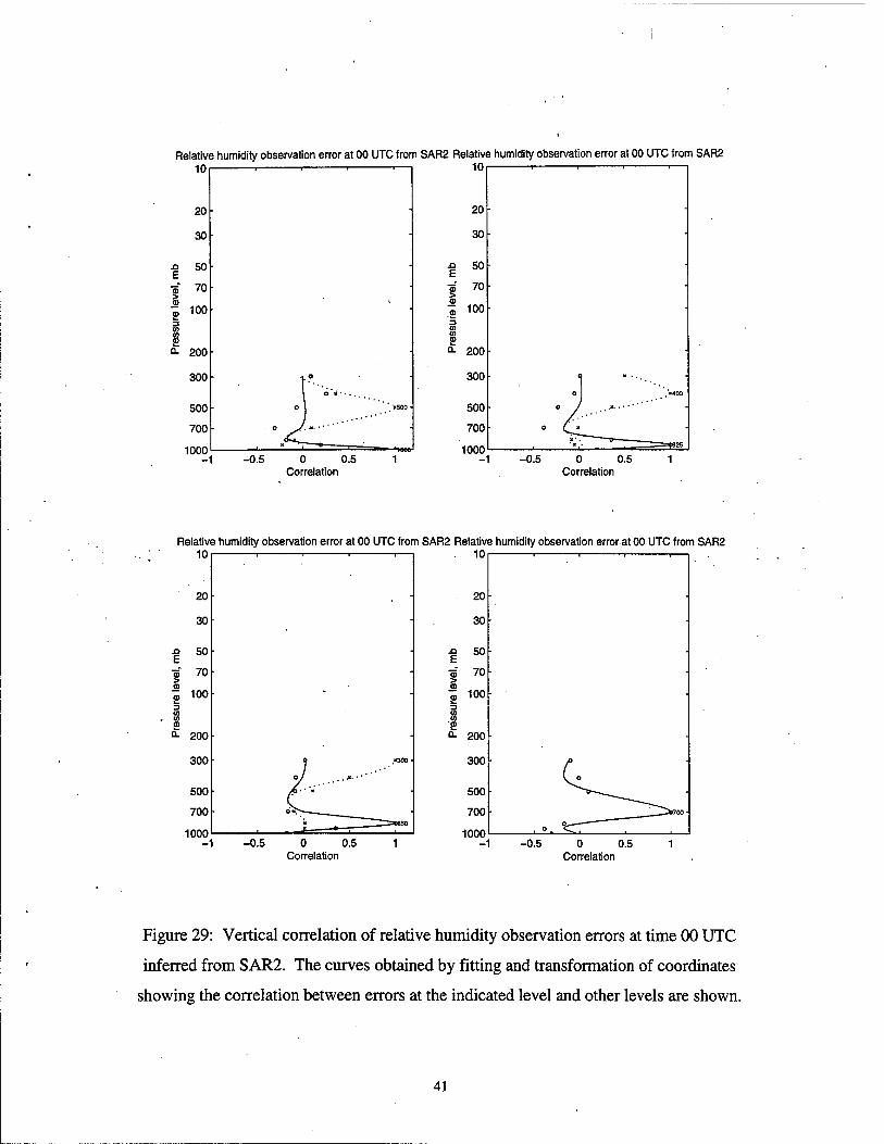
Figure 29: Vertical correlation of relative humidity observation errors at time 00 UTC
inferred from SAR2. The curves obtained by fitting and transformation of coordinates
showing the correlation between errors at the indicated level and other levels are shown.
41
Relative humidity observation error at 00 UTC from FAR3 Relative humidity observation error at 00 UTC from FAR3 10| 1 ■ 1 , 1 10r
-0.5 0 0.5 Correlation
-0.5 0 0.5 Correlation
Relative humidity observation error at 00 UTC from FAR3 Relative humidity observation error at 00 UTC from FAR3 10,— . . . ,—r 10r
-0.5 0 0.5 Correlation
-0.5 0 0.5 1 Correlation
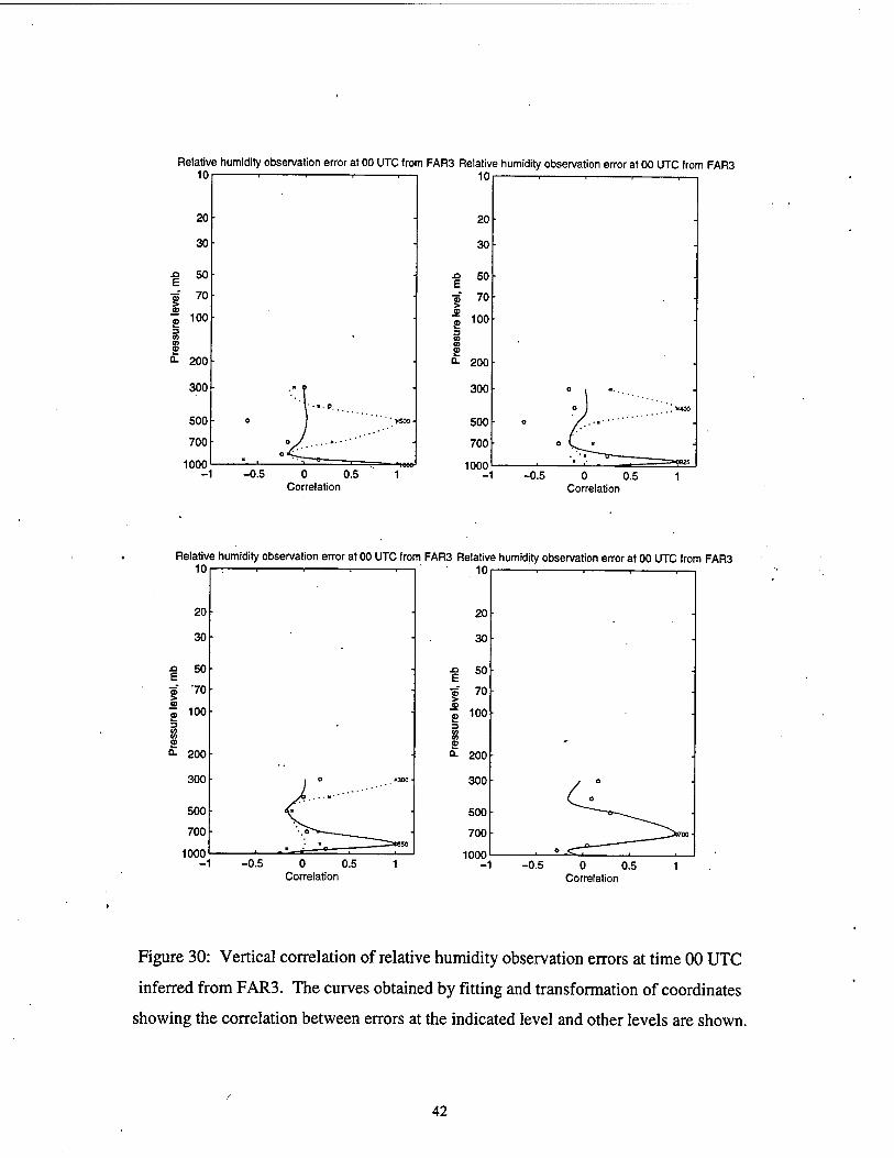
Figure 30: Vertical correlation of relative humidity observation errors at time 00 UTC
inferred from FAR3. The curves obtained by fitting and transformation of coordinates
showing the correlation between errors at the indicated level and other levels are shown.
42
Relative humidity observation error at 12 UTC from SAR2 Relative humidity observation error at 12 UTC from SAR2 10, . r , r—, 10r
-0.5 . 0 0.5 Correlation
-0.5 0 0.5 1 Correlation
Relative humidity observation error at 12 UTC from SAR2 Relative humidity observation error at 12 UTC from SAR2 10i . 1 . ,—, 10r
-0.5 0 0.5 Correlation
-0.5 0 0.5 1 ' Correlation
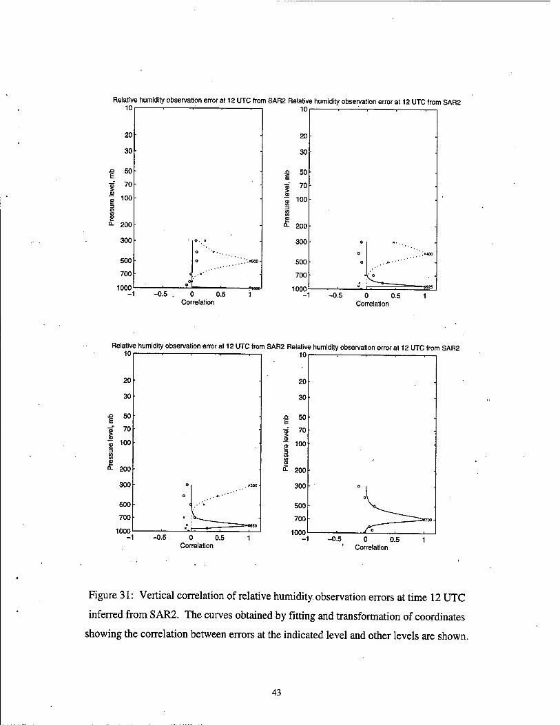
Figure 31: Vertical correlation of relative humidity observation errors at time 12 UTC
inferred from S AR2. The curves obtained by fitting and transformation of coordinates
showing the correlation between errors at the indicated level and other levels are shown.
43
Relative humidity observation error at 12 UTC from FAR3 Relative humidity observation error at 12 UTC from FAR3 10f . , , , , 10
E
I £
20
30
50
70
100
£ 200
300
500
700
1000 -1
C -0.5 0 0.5
Correlation -0.5 0 0.5 1
Correlation
Relative humidity observation error at 12 UTC from FAR3 Relative humidity observation error at 12 UTC from FAR3 10| . r^ , ,—, ■ ior
20
30
n E
50
9 70
100
a. 200
300
-0.5 0 0.5 Correlation
-0.5 0 0.5 1 Correlation
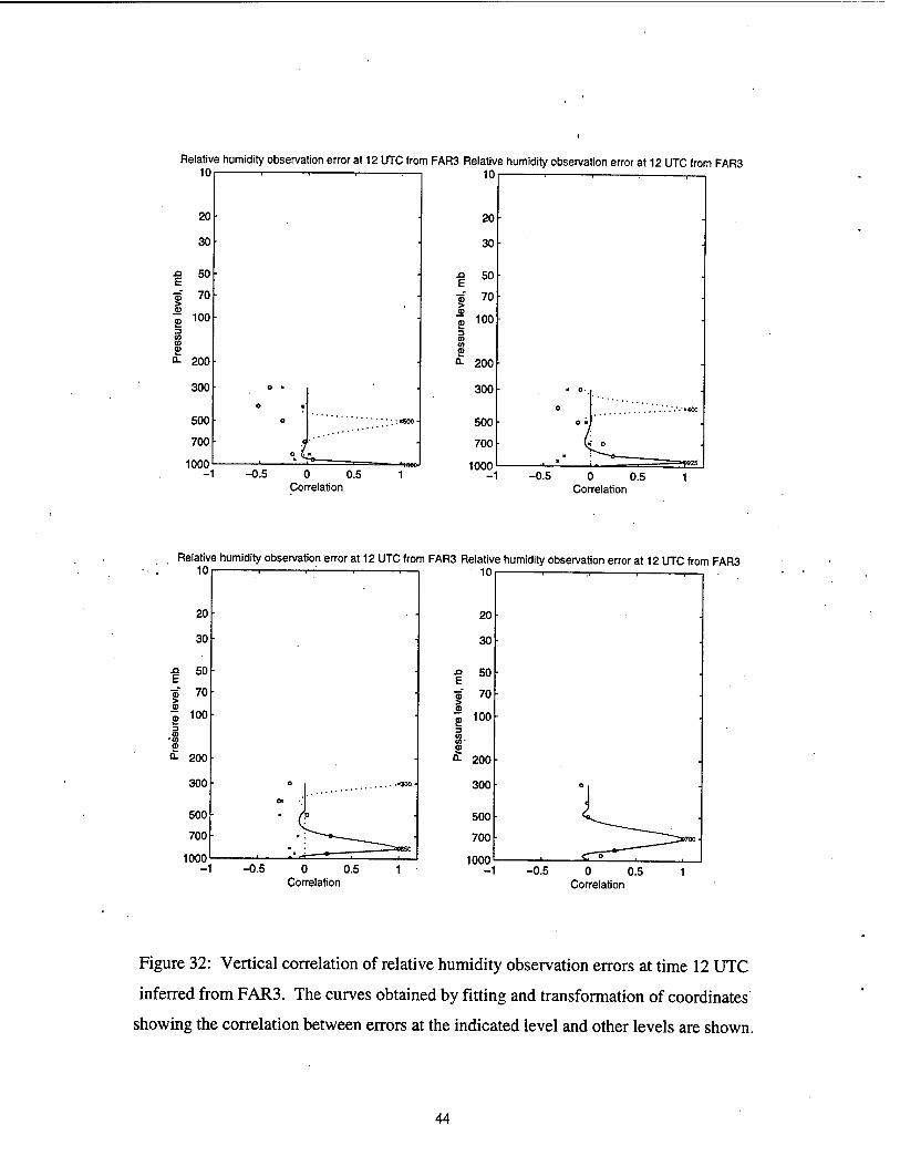
Figure 32: Vertical correlation of relative humidity observation errors at time 12 UTC
inferred from FAR3. The curves obtained by fitting and transformation of coordinates
showing the correlation between errors at the indicated level and other levels are shown.
44
10
20
30
50
E 70
3 100 CO w £ 0.
200
300
500 •
700
1000
Temperature using SAR2 10
Temperature using FAR3
20
30
50 00UTC
12UTC
Pre
ssur
e, m
b
8 3
200
300
500
700
0.05 0.1 0.15 0.2 Correlation distance, radians
0.25 1000
0.05 0.1 0.15 0.2 Correlation distance, radians
0.25
10
20
30
50
70
100-
200
Relative humidity using SAR2
0.05 0.1 0.15 0.2 Correlation distance, radians
0.25
10 Relative humidity using FAR3
20
30
50 00UTC
12UTC
Pre
ssur
e, m
b
s a
200
300
500
700
1000
0OUTC
12UTC
0.05 0.1 0.15 0.2 Correlation distance, radians
0.25
Figure 33: Correlation distance values for spatial covariance fits for
temperature and relative humidity prediction errors using SAR2 and
FAR3 fits at 00 and 12 UTC.
45
Binned rh(850)&temperature(925) errors; SAR2 0.04
Binned rh(850)&temperature(850) errors; SAR2 0.15 r
02 0.4 0.6 Distance, radians
Binned rh(850)&temperature(700) errors: SAR2 0.08 r
8 t e ü
0.2 0.4 0.6 Distance, radians
Binned rh(850)&temperature(500) errors; SAR2 0.021 1 1 .
I -0.01 e o
0.2 0.4 0.6 Distance, radians
-0.02
-0.03
° Ow ° o
0.2 0.4 0.6 Distance, radians
0.8
Figure 34: Binned cross-covariances between relative humidity error
at 850 mb level and temperature error at 925, 850,700, and 500 mb
at time 00 UTC. Also shown are the SAR2 fits to the data.
46
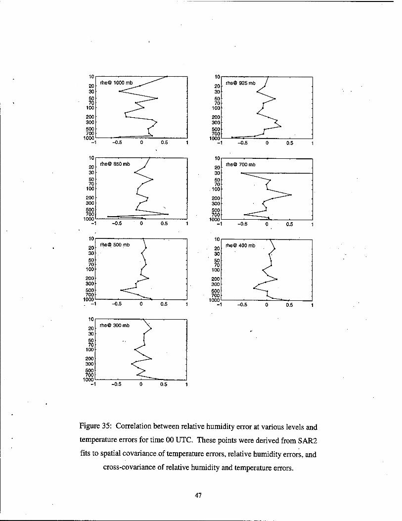
Figure 35: Correlation between relative humidity error at various levels and
temperature errors for time 00 UTC. These points were derived from S AR2
fits to spatial covariance of temperature errors, relative humidity errors, and
cross-covariance of relative humidity and temperature errors.
47
500 700
1000
Figure 36: Correlation between relative humidity error at various levels and
temperature errors for time 12 UTC. These points were derived from SAR2
fits to spatial covariance of temperature errors, relative humidity errors, and
cross-covariance of relative humidity and temperature errors.
48
0.5 1
Figure 37: Correlation between relative humidity error at various levels and
temperature errors for time 00 UTC. These points were derived from FAR3
fits to spatial covariance of temperature errors, relative humidity errors, and
cross-covariance of relative humidity and temperature errors.
49
500 700
1000
Figure 38: Correlation between relative humidity error at various levels and
temperature errors for time 12 UTC. These points were derived from FAR3
fits to spatial covariance of temperature errors, relative humidity errors, and
cross-covariance of relative humidity and temperature errors.
50
Temp(925mb) - rel. hum.(850mb) FAR3 St at 00 UTC Temp(850mb) - rat. hum.(850mb) FAR3 fit at 00 UTC 10r
0.2 0.4 0.6 Distance, radians
0.2 0.4 0.6 Distance, radians
Temp(700mb) - rel. hum.(850mb) FAR3 tit at 00 UTC Temp(500mb) - rel. hum.(850mb) FAR3 fit at 00 UTC 5, . , . 1 8r
0.2 0.4 0.6 Distance, radians
0.2 0.4 0.6 Distance, radians
Figure 39: Binned covariances of the difference between normalized relative
humidity error at 850 mb level and normalized temperature error at 925, 850,
700, and 500 mb at time 00 UTC. Also shown are the FAR3 fits to the data.
51
0.5 1
Figure 40: Correlation between temperature error at various heights and relative
humidity error at the indicated heights for time 00 UTC. These curves were derived
using the difference method and SAR2 fits to the spatial covariance data.
52
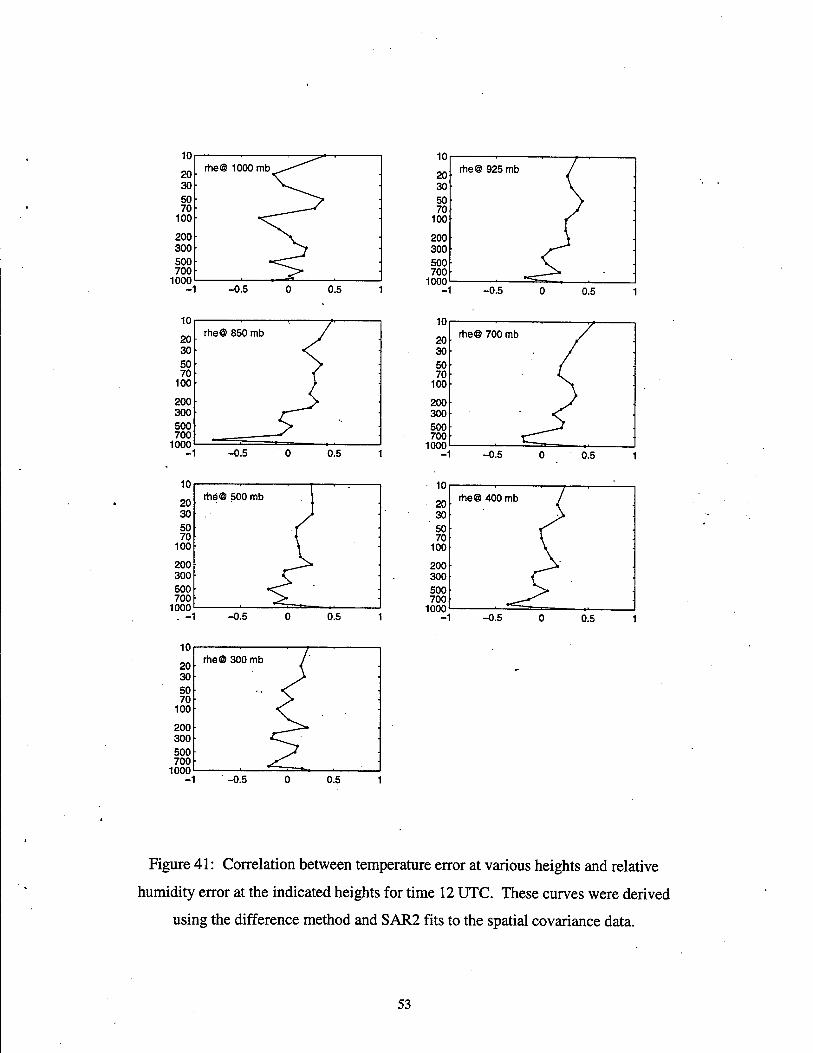
Figure 41: Correlation between temperature error at various heights and relative
humidity error at the indicated heights for time 12 UTC. These curves were derived
using the difference method and SAR2 fits to the spatial covariance data.
53
500 700
1000
Figure 42: Correlation between temperature error at various heights and relative
humidity error at the indicated heights for time 00 UTC. These curves were derived
using the difference method and FAR3 fits to the spatial covariance data.
54
500 h 700
1000
Figure 43: Correlation between temperature error at various heights and relative
humidity error at the indicated heights for time 12 UTC. These curves were derived
using the difference method and FAR3 fits to the spatial covariance data.
55
20 l 30 ( 50 \ 70 [
100 ( 200 <^ 300 / 500 /-_______^ 700 !^=—70C
20 1 30 L SO j> 70 j—
100 <f 200 \ 300 ^~3n^=="<300
500 <^" 700 ?
20 / 30 ^ SO ^^
\ 70 S*^
% 100 \ s /
200
300
500 700
^~ ■«"
20 /• . 30 )
i 70 § 100 : *• 200
TZ-----=:>"70
300 \. 500 \ 700 s>
20
30 ^_^üi>90
• * i 70 S 100
5 ft 200
300
500 700
4 70
20
30 1 _ % so ^^> * 70 /^ | 100
"■ 200 \ 300 / 500 c 700 V
Figure 44: Vertical correlation curves for temperature prediction error at 00
UTC as derived from the S AR2 approximations. Each of the sixteen curves
shows the correlation between the error at the indicated level and other levels.
56
20 1 30 )
■ü 50 I 70 ( 1 100
£ 200 I
300 ) 500 / 700 C^_^__^ *-_T~ i im
20 \ 30 ) 50 / 70 ^\
100 ) 200 \ 300 \ 500 \ 700 ' -Tnn
20
30
s "> J 70 ( I 1O0
"■ 200 )
300 ^^^^ • 500 "~^>>500 700 <--^'
20 \ 30 <^
s so ^^ 1 70 / S 100 S 1 200
^_^^=«-15C f
300 ( 500 ) 700 ^
Figure 45: Vertical correlation curves for temperature observation error at 00
UTC as derived from the S AR2 approximations. Each of the sixteen curves
shows the correlation between the error at the indicated level and other levels.
57
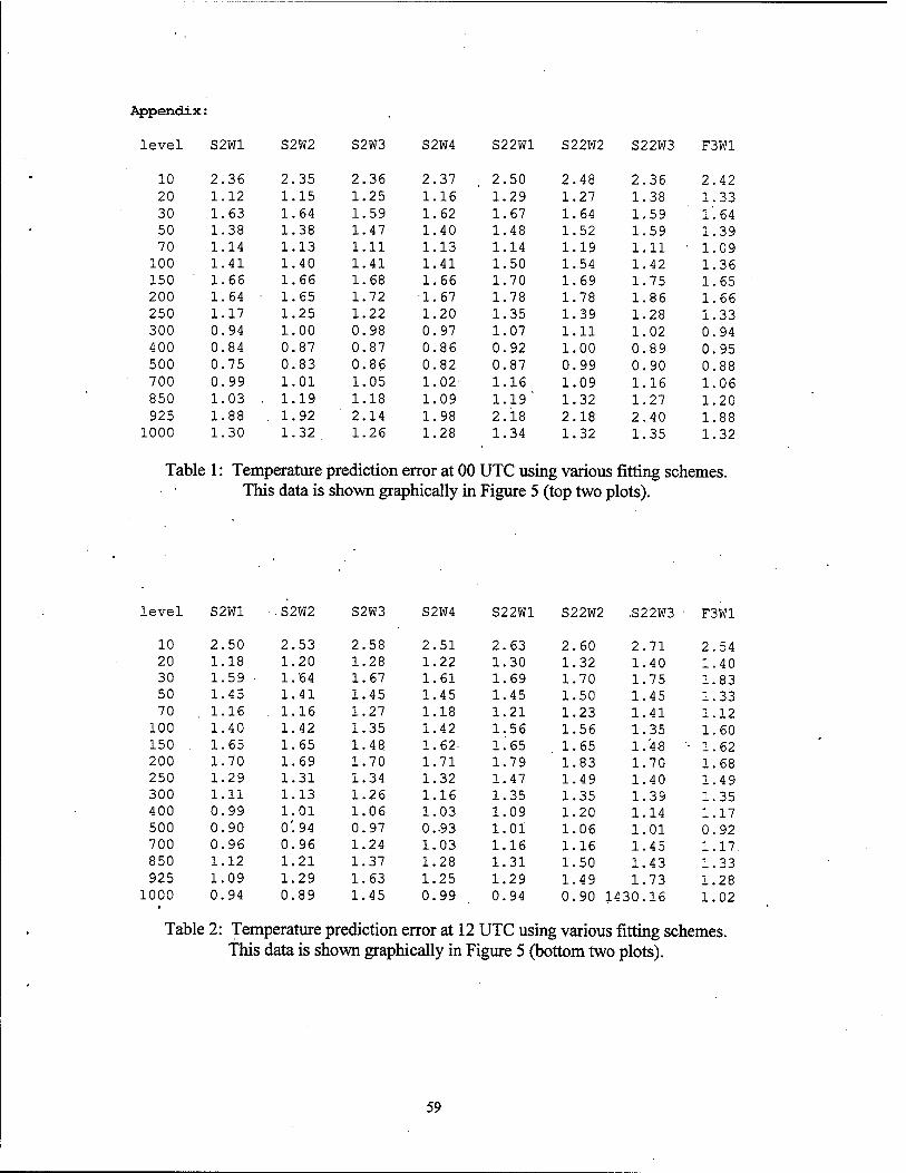
Appendix ;
level S2W1 S2W2 S2W3 S2W4 S22W1 S22W2 S22W3 F3W1
10 2.36 2.35 2.36 2.37 2.50 2.48 2.36 2.42 20 1.12 1.15 1.25 1.16 1.29 1.27 1.38 1.33 30 1.63 1.64 1.59 1.62 1.67 1.64 1.59 1.64 50 1.38 1.38 1.47 1.40 1.48 1.52 1.59 1.39 70 1.14 1.13 1.11 1.13 1.14 1.19 1.11 1.09
100 1.41 1.40 1.41 1.41 1.50 1.54 1.42 1.36 150 1.66 1.66 1.68 1.66 1.70 1.69 1.75 1.65 200 1.64 • 1.65 1.72 1.67 1.78 1.78 1.86 1.66 250 1.17 1.25 1.22 1.20 1.35 1.39 1.28 1.33 300 0.94 1.00 0.98 0.97 1.07 1.11 1.02 0.94 400 0.84 0.87 0.87 0.86 0.92 1.00 0.89 0.95 500 0.75 0.83 0.86 0.82 0.87 0.99 0.90 0.88 700 0.99 1.01 1.05 1.02 1.16 1.09 1.16 1.06 850 1.03 1.19 1.18 1.09 1.19 ' 1.32 1.27 1.20 925 1.88 . 1.92 2.14 1.98 2.18 2.18 2.40 1.88
1000 1.30 1.32, 1.26 1.28 1.34 1.32 1.35 1.32
Table 1: Temperature prediction error at 00 UTC using various fitting schemes. This data is shown graphically in Figure 5 (top two plots).
level S2W1 .S2W2 S2W3 S2W4 S22W1 S22W2 .S22W3 F3W1
10 2.50 2.53 2.58 2.51 2.63 2.60 2.71 2.54 20 1.18 1.20 1.28 1.22 1.30 1.32 1.40 1.40 30 1.59 • 1/64 1.67 1.61 1.69 1.70 1.75 1.83 50 1.45 1.41 1.45 1.45 1.45 1.50 1.45 1.33 70 . 1.16 . 1.16 1.27 1.18 1.21 1.23 1.41 1.12
100 1.40 1.42 1.35 1.42 1.56 1.56 1.35 1.60 150 . 1.65 1.65 1.48 1.62- 1.65 . 1.65 1.48 • 1.62 200 1.70 1.69 1.70 1.71 1.79 1.83 1.70 1.68 250 1.29 1.31 1.34 1.32 1.47 1.49 1.40 1.49 300 1.11 1.13 1.26 1.16 1.35 1.35 1.39 1.35 400 0.99 1.01 1.06 1.03 1.09 1.20 1.14 1.17 500 0.90 0'.94 0.97 0.-93 1.01 1.06 1.01 0.92 700 0.96 0.96 1.24 1.03 1.16 1.16 1.45 1.17 850 1.12 . 1.21 1.37 1.28 1.31 1.50 1.43 1.33 925 1.09 1.29 1.63 1.25 1.29 1.49 1.73 1.28
1000 0.94 0.89 1.45 0.99 , 0.94 0.90 1430.16 1.02
Table 2: Temperature prediction error at 12 UTC using various fitting schemes. This data is shown graphically in Figure 5 (bottom two plots).
59
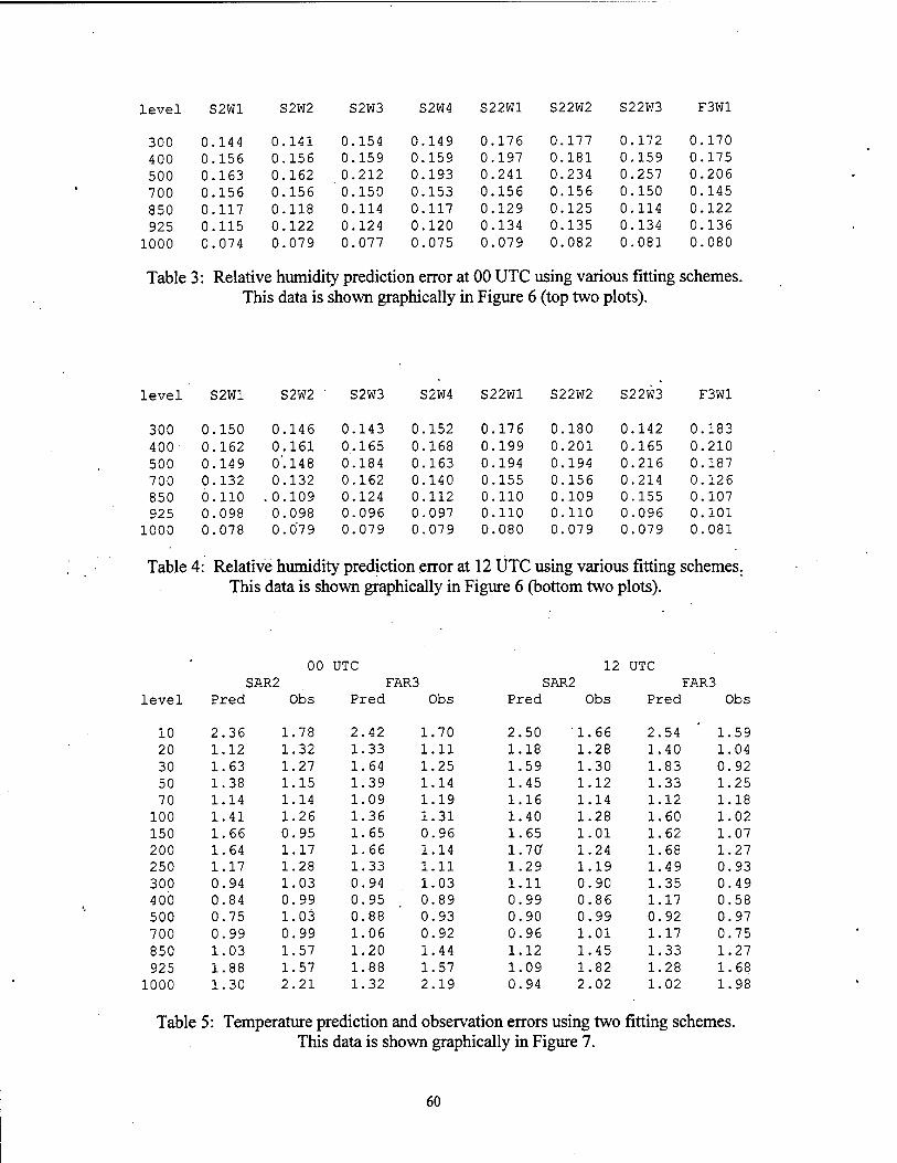
level S2W1 S2W2 S2W3 S2W4 S22W1 S22W2 S22W3 F3W1
300 0.144 0.141 0.154 0 149 0.176 0.177 0 172 0 170 400 0.156 0.156 0.159 0 159 0.197 0.181 0 159 0 175 500 0.163 0.162 0.212 0 193 0.241 0.234 0 257 0 206 700 0.156 0.156 0.150 0 153 0.156 0.156 0 150 0 145 850 0.117 0.118 0.114 0 117 0.129 0.125 0 114 0 122 925 0.115 0.122 0.124 0 120 0.134 0.135 0 134 0 136
1000 0.074 0.079 0.077 0 075 0.079 0.082 0 081 0 080
Table 3: Relative humidity prediction error at 00 UTC using various fitting schemes. This data is shown graphically in Figure 6 (top two plots).
level S2W1 S2W2 S2W3 S2W4 S22W1 S22W2 S22W3 F3W1
300 0 150 0 146 0.143 0.152 0.176 0.180 0.142 0.183 400 0 162 0 161 0.165 0.168 0.199 0.201 0.165 0.210 500 0 149 0' 148 0.184 0.163 0.194 0.194 0.216 0.187 700 0 132 0 132 0.162 0.140 0.155 0.156 0.214 0.126 850 0 110 . 0 109 0.124 0.112 0.110 0.109 0.155 0.107 925 0 098 0 098 0.096 0.097 0.110 0.110 0.096 0.101
1000 0 078 0 079 0.079 0.079 0.080 0.079 0.079 0.081
Table 4: Relative humidity prediction error at 12 UTC using various fitting schemes. This data is shown graphically in Figure 6 (bottom two plots).
level
00 UTC SAR2 FAR3
Pred Obs Pred Obs
12 UTC SAR2 FAR3
Pred Obs Pred Obs
10 2.36 1.78 2.42 1.70 2.50 1.66 2.54 1.59 20 1.12 1.32 1.33 1.11 1.18 1.28 1.40 1.04 30 1.63 1.27 1.64 1.25 1.59 1.30 1.83 0.92 50 1.38 1.15 1.39 1.14 1.45 1.12 1.33 1.25 70 1.14 1.14 1.09 1.19 1.16 1.14 1.12 1.18
100 1.41 1.26 1.36 1.31 1.40 1.28 1.60 1.02 150 1.66 0.95 1.65 0.96 1.65 1.01 1.62 1.07 200 1.64 1.17 1.66 1.14 1.70 1.24 1.68 1.27 250 1.17 1.28 1.33 1.11 1.29 1.19 1.49 0.93 300 0.94 1.03 0.94 1.03 1.11 0.90 1.35 0.49 400 0.84 0.99 0.95 0.89 0.99 0.86 1.17 0.58 500 0.75 1.03 0.88 0.93 0.90 0.99 0.92 0.97 700 0.99 0.99 1.06 0.92 0.96 1.01 1.17 0.75 850 1.03 1.57 1.20 1.44 1.12 1.45 1.33 1.27 925 1.88 1.57 1.88 1.57 1.09 1.82 1.28 1.68
1000 1.30 2.21 1.32 2.19 0.94 2.02 1.02 1.98
Table 5: Temperature prediction and observation errors using two fitting schemes. This data is shown graphically in Figure 7.
60
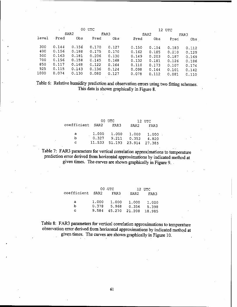
00 UTC 12 UTC SAR2 FAR3 SAR2 FAR3
level Pred Obs Pred Obs Pred Obs Pred Obs
300 0.144 0.156 0.170 0.127 0.150 0.154 0.183 0 112 400 0.156 0.188 0.175 0.170 0.162 0.185 0.210 0 129 500 0.163 0.181 0.206 0.130 0.149 0.203 0.187 0 169 700 0.156 0.158 0.145 0.168 0.132 0.181 0.126 0 186 850 0.117 0.168 0.122 0.164 0.110 0.173 0.107 0 174 925 0.115 0.143 0.136 0.124 0.098 0.144 0.101 0 142
1000 0.074 0.130 0.080 0.127 0.078 0.112 0.081 0 110
Table 6: Relative humidity prediction and observation errors using two fitting schemes. This data is shown graphically in Figure 8.
00 UTC 12 UTC coefficient SAR2 FAR3 SAR2 FAR3
a 1.000 1.000 1.000 1.000 b 0.327 9.211 0.353 4.820 c 11.533 51.193 23.914 27.385
Table 7: FAR3 parameters for vertical correlation approximations to temperature prediction error derived from horizontal approximations by indicated method at
given times. The curves are shown graphically in Figure 9. ■
00 -UTC 12 UTC coefficient SAR2 FAR3 SAR2 FAR3
a 1.000 1.000 1.000 1.000 b 0.378 5.968 0.356 5.398 c 9.584 45.270 21.208 18.985
Table 8: FAR3 parameters for vertical correlation approximations to temperature observation error derived from horizontal approximations by indicated method at
given times. The curves are shown graphically in Figure 10.
61
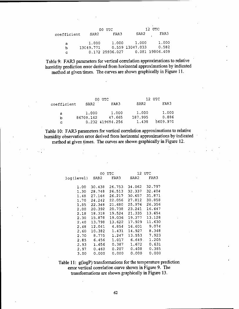
00 UTC 12 UTC coefficient SAR2 FAR3 SAR2 _ FAR3
a 1.000 1.000 1.000 1.000 b 13049.771 0.559 13047.033 0.582 c 0.172 25936.027 0.081 19806.409
Table 9: FAR3 parameters for vertical correlation approximations to relative humidity prediction error derived from horizontal approximations by indicated
method at given times. The curves are shown graphically in Figure 11.
00 UTC 12 UTC fficient SAR2 FAR3 SAR2 FAR3
a 1.000 1.000 1.000 1.000 b 86709.162 47.665 187.995 0.886 c 0.232 419684.256 1.438 5609.970
Table 10: FARS parameters for vertical correlation approximations to relative humidity observation error derived from horizontal approximations by indicated
method at given times. The curves are shown graphically in Figure 12.
00 UTC 12 UTC (level) SAR2 FAR3 SAR2 FAR3
1.00 30.438 26.753 34.062 32.797 1.30 28.748 26.513 32.337 32.404 1.48 27.164 26.217- 30.657 31.871 1.70 24.242 22.056 27.812 30.858 1.85 22.348 21.680 25.976 26.356 2.00 20.392 20.738 23.241 16.647 2.18 18.318 19.524 21.335 13.654 2.30 15.878 19.036 19.377 13.128 2.40 13.798 13.622 17.929 11.630 2.48 12.041 4.854 16.601 9.074 2.60 10.382 1.431 14.927 8.348 2.70 8.775 1.247 13.553 7.923 2.85 6.456 1.017 6.649 1.205 2.93 1.656 0.387 1.672 0.631 2.97 0.460 0.207 0.408 0.385 3.00 0.000 0.000 0.000 0.000
Table 11: g(logP) transformations for the temperature prediction error vertical correlation curve shown in Figure 9. The
transformations are shown graphically in Figure 13.
62
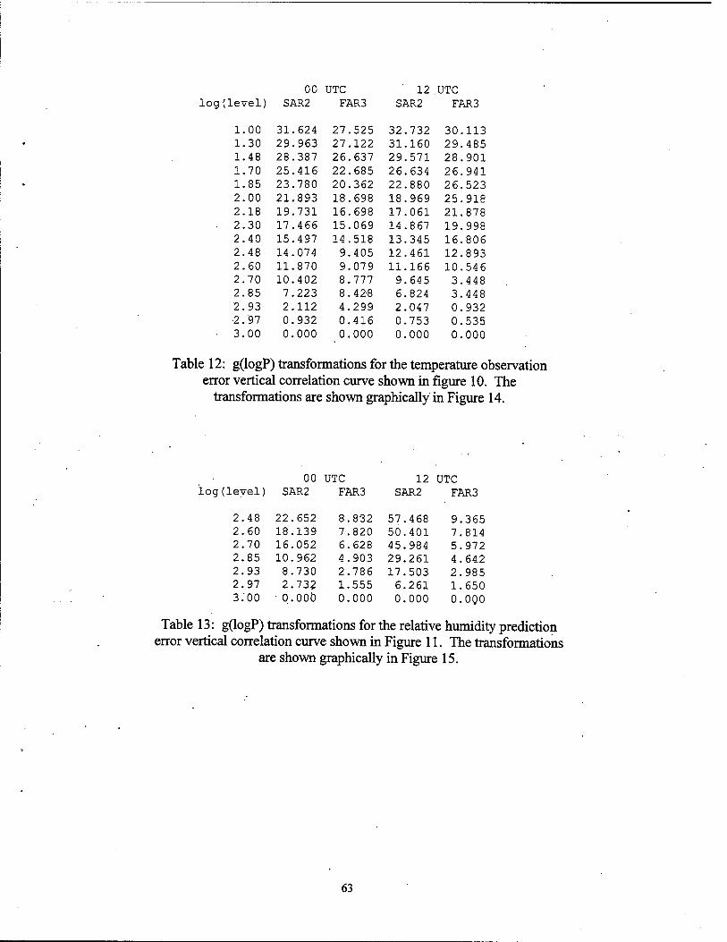
00 UTC 12 UTC log(level) SAR2 FAR3 SAR2 FAR3
1.00 31.624 27.525 32.732 30.113 1.30 29.963 27.122 31.160 29.485 1.48 28.387 26.637 29.571 28.901 1.70 25.416 22.685 26.634 26.941 1.85 23.780 20.362 22.880 26.523 2.00 21.893 18.698 18.969 25.918 2.18 19.731 16.698 17.061 21.878 2.30 17.466 15.069 14.867 19.998 2.40 15.497 14.518 13.345 16.806 2.48 14.074 9.405 12.461 12.893 2.60 11.870 9.079 11.166 10.546 2.70 10.402 8.777 9.645 3.448 2.85 7.223 8.42-8 6.824 3.448 2.93 2.112 4.299 2.047 0.932 •2.97 0.932 0.416 0.753 0.535 3.00 0.000 0.000 0.000 0.000
Table 12: g(logP) transformations for the temperature observation error vertical correlation curve shown in figure 10. The
transformations are shown graphically in Figure 14.
00 UTC 12 UTC log(level) SAR2 FAR3 SAR2 FAR3
2.48 22.652 8.832 57.468 9.365 2.60 18.139 7.820 50.401 7.814 2.70 16.052 6.628 45.984 5.972 2.85 10.962 4.903 29.261 4 . 64.2 2.93 8.730 2.786 17.503 2.985 2.97 2.732 1.555 6.261 1.650 3.'00 ■ 0.000 0.000 0.000 0.000
Table 13: g(logP) transformations for the relative humidity prediction error vertical correlation curve shown in Figure 11. The transformations
are shown graphically in Figure 15.
63
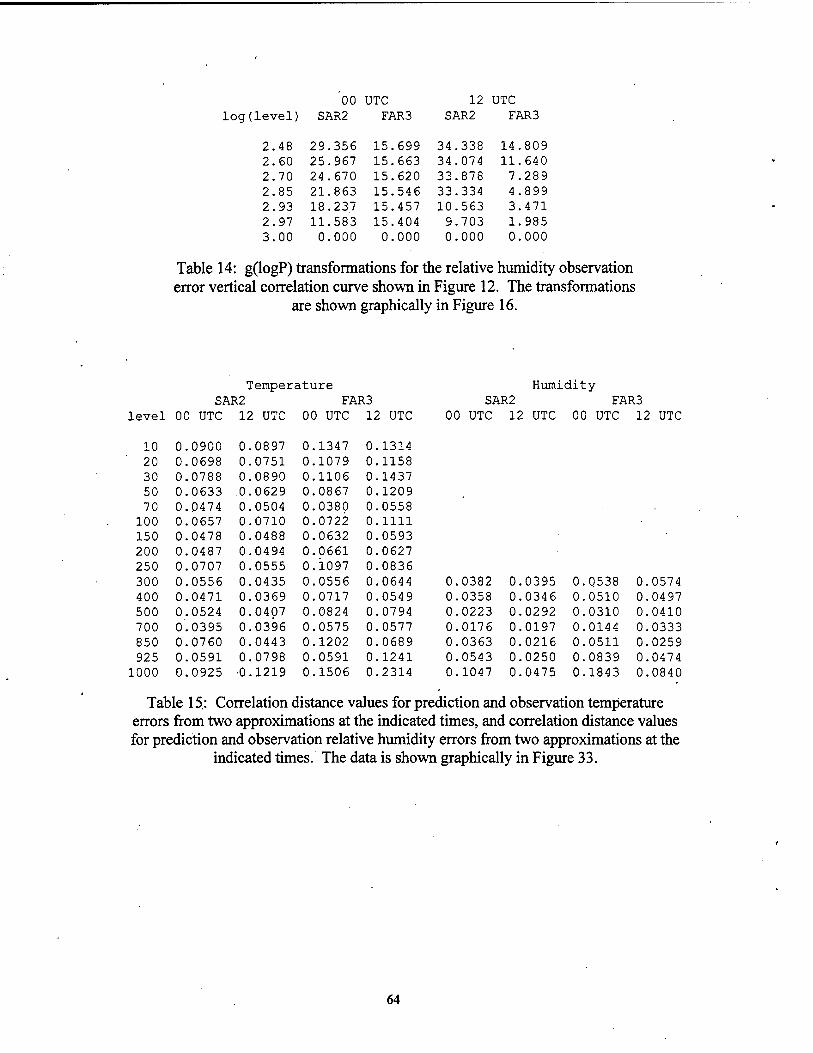
00 UTC 12 UTC log(level) SAR2 FAR3 SAR2 FAR3
2.48 29.356 15.699 34.338 14.809 2.60 25.967 15.663 34.074 11.640 2.70 24.670 15.620 33.878 7.289 2.85 21.863 15.546 33.334 4.899 2.93 18.237 15.457 10.563 3.471 2.97 11.583 15.404 9.703 1.985 3.00 0.000 0.000 0.000 0.000
Table 14: g(logP) transformations for the relative humidity observation error vertical correlation curve shown in Figure 12. The transformations
are shown graphically in Figure 16.
Temperature Humidity SAR2 FAR3 SAR2 FAR3
level 00 UTC 12 UTC 00 UTC 12 UTC 00 UTC 11 i UTC 00 UTC 12 UTC
10 0.0900 0.0897 0.1347 0.1314 20 0.0698 0.0751 0.1079 0.1158 30 0.0788 0.0890 0.1106 0.1437 50 0.0633 .0.0629 0.0867 0.1209 70 0.0474 0.0504 0.0380 0.0558
100 0.0657 0.0710 0.0722 0.1111 150 0.0478 0.0488 0.0632 0.0593 200 0.0487 0.0494 0.0661 0.0627 250 0.0707 0.0555 0.1097 0.0836 300 0.0556 0.0435 0.0556 0.0644 0 0382 0. 0395 0.0538 0 0574 400 0.0471 0.0369 0.0717 0.0549 0 0358 0 0346 0.0510 0 0497 500 0.0524 0.0407 0.0824 0.0794 0 0223 0 0292 0.0310 0 0410 700 0.0395 0.0396 0.0575 0.0577 0 0176 0 0197 0.0144 0 0333 850 0.0760 0.0443 0.1202 0.0689 0 0363 0 0216 0.0511 0 0259 925 0.0591 0.0798 0.0591 0.1241 0 0543 0 0250 0.0839 0 0474
1000 0.0925 •0.1219 0.1506 0.2314 0 1047 0 0475 0.1843 0 0840
Table 15: Correlation distance values for prediction and observation temperature errors from two approximations at the indicated times, and correlation distance values for prediction and observation relative humidity errors from two approximations at the
indicated times. The data is shown graphically in Figure 33.
64
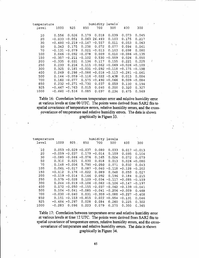
temperat ure humidity levels' level 1000 925 850 700 500 400 300
10 0.556 0.026 0.179 0.018 0.039 0.073 0.045 20 -0.033 -0.051 0.063 26.493 0.103 0.175 0.217 30 -0.480 -0.219 -0.147 -0.557 0.011 0.053 0.063 50 0.343 0.175 0.238 0.072 0.077 0.094 0.061 70 -0.131 -0.079 0.021 -0.013 0.103 0.098 0.080
100 0.046 -0.092 -0.078 0.009 0.010 -0.086 -0.135 150 -0.357 -0.211 -0.102 0.530 -0.009 0.026 0.050 200 -0.335 0.031 0.136 0.117 0.155 0.221 0.225 250 0.233 0.216 0.111 -0.062 -0.069 -0.026 -0.109 300 0.325 0.181 -0.031 -0.092 -0.118 -0.175 -0.198 400 0.249 0.298 -0.086 -0.018 -0.113 -0.281 -0.061 500 0.144 -0.059 -0.116 -0.022 -0.438 0.013 0.084 700 0.160 -0.077 0.575 -0.490 -0.066 0.009 -0.084 850 0.232 -0.271 -0.730 0.037 0.059 0.130 0.194 925 -0.467 -0.763 0.015 0.040 0.200 0.320 0.327
1000 -0.660 -0.516 0.085 0.097 0.234 0.475 0.569
Table 16: Correlation between temperature error and relative humidity error at various levels at time 00 UTC. The points were derived from SAR2 fits to
spatial covariance of temperature errors, relative humidity errors, and the cross- covariance of temperature and relative humidity errors. The data is shown
graphically in Figure 33.
temperature humidity levels level 1000 925 • 850 '700 500 400 300
10 0.053 -0.029 -0.037 0.080 0.033 0.017 -0.013 20 -0.059 -0.037 0.179 -0.014 0.109 0.095 0.104 30 -0.080 -0.046 -0.076 0.165 0.024 0.072 0.079 50 0.310 0.021 0.030 0.018 0.013 0.026 -0.080 70 , 0.148 -0.006 5.790 -0.050 0.071 0.032 0.043
100 0.061. -0.017 0.087 -0.040 -0.118 -0.128 -0.202 150 -0.112 0.176 -0.022 0.089 0.048 0.050 0.027 200 -0.119 -0.014 0.146 0.092 0.196 0.184 0.215 250 0.175 -0.028 0.109 -0.034 -0.117 -0.085 -0.159 300 0.244 -0.019 -0.106 -0.062 -0..106 -0.147 -0.197 400 0.172 -0.050 -0.155 -0.037 -0.062 -0.139 -0.041 500 0.104 -0.041 -0.085 -0.041 -0.206 -0.009 0.468 700 -0.030 -0.040 0.031 -0.359 -0.088 -0.227 -0.408 850 0.151 -0.153 -0.815 0.022 -0.054 -0.131 0.046 925 -0.484 -0.297 0.028 0.084 0.260 0.225 0.302
1000 -0.283 0.096 0.223 0.079 0.275 0.300 0.365
Table 17: Correlation between temperature error and relative humidity error at various levels at time 12 UTC. The points were derived from SAR2 fits to
spatial covariance of temperature errors, relative humidity errors, and the cross- covariance of temperature and relative humidity errors. The data is shown
graphically in Figure 34.
65
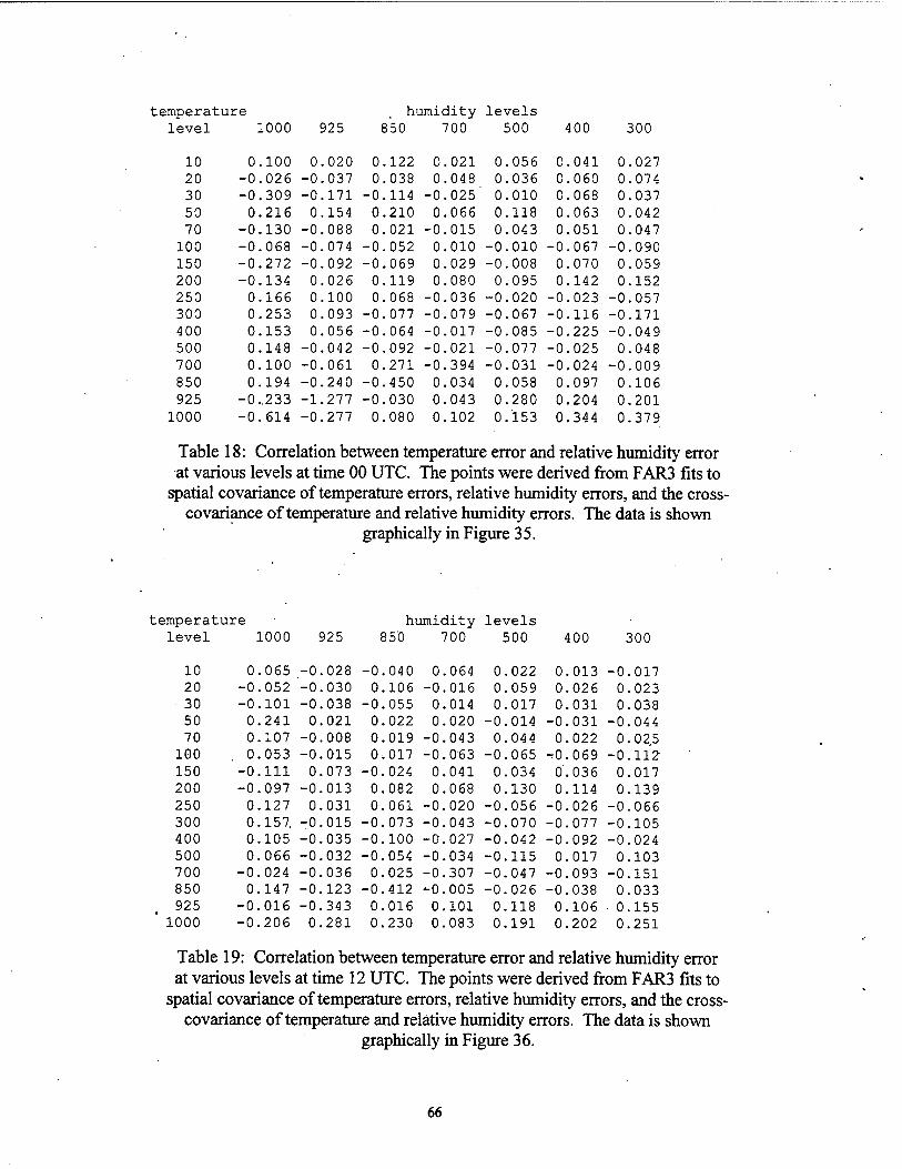
temperati are humidity levels level 1000 925 850 700 500 400 300
10 0.100 0.020 0.122 0.021 0.056 0.041 0.027 20 -0.026 -0.037 0.038 0.048 0.036 0.060 0.074 30 -0.309 -0.171 -0.114 -0.025' 0.010 0.068 0.037 50 0.216 0.154 0.210 0.066 0.118 0.063 0.042 70 -0.130 -0.088 0.021 -0.015 0.043 0.051 0.047
100 -0.068 -0.074 -0.052 0.010 -0.010 -0.067 -0.090 150 -0.272 -0.092 -0.069 0.029 -0.008 0.070 0.059 200 -0.134 0.026 0.119 0.080 0.095 0.142 0.152 250 0.166 0.100 0.068 -0.036 -0.020 -0.023 -0.057 300 0.253 0.093 -0.077 -0.079 -0.067 -0.116 -0.171 400 0.153 0.056 -0.064 -0.017 -0.085 -0.225 -0.049 500 0.148 -0.042 -0.092 -0.021 -0.077 -0.025 0.048 700 0.100 -0.061 0.271 -0.394 -0.031 -0.024 -0.009 850 0.194 -0.240 -0.450 0.034 0.058 0.097 0.106 925 -0..233 -1.277 -0.030 0.043 0.280 0.204 0.201
1000 -0.614 -0.277 0.080 0.102 0.153 0.344 0.379
Table 18: Correlation between temperature error and relative humidity error at various levels at time 00 UTC. The points were derived from FAR3 fits to
spatial covariance of temperature errors, relative humidity errors, and the cross- covariance of temperature and relative humidity errors. The data is shown
graphically in Figure 35.
temperature humidity levels level 1000 925 850 700 500 400 300
10 0.065 .-0.028 -0.040 0.064 0.022 0.013 -0.017 20 -0.052 -0.030 0.106 -0.016 0.059 0.026 0.023 30 -0.101 -0.038 -0.055 0.014 0.017 0.031 0.038 50 0.241 0.021 0.022 0.020 -0.014 -0.031 -0.044 70 0.107 -0.008 0.019 -0.043 0.044 0.022 0.02.5
100 0.053 -0.015 0.017 -0.063 -0.065 -.0.069 -0.112 150 -0.111 0.073 -0.024 0.041 0.034 0.036 0.017 200 -0.097 -0.013 0.082 0.068 0.130 0.114 0.139 250 0.127 0.031 0.061 -0.020 -0.056 -0.026 -0.066 300 0.157, -0.015 -0.073 -0.043 -0.070 -0.077 -0.105 400 0.105 -0.035 -0.100 -0.027 -0.042 -0.092 -0.024 500 0.066 -0.032 -0.054 -0.034 -0.115 0.017 0.103 700 -0.024 -0.036 0.025 -0.307 -0.047 -0.093 -0.151 850 0.147 -0.123 -0.412 -0.005 -0.026 -0.038 0.033 925 -0.016 -0.343 0.016 0.101 0.118 0.106 • 0.155
' 1000 -0.206 0.281 0.230 0.083 0.191 0.202 0.251
Table 19: Correlation between temperature error and relative humidity error at various levels at time 12 UTC. The points were derived from FAR3 fits to
spatial covariance of temperature errors, relative humidity errors, and the cross- covariance of temperature and relative humidity errors. The data is shown
graphically in Figure 36.
66
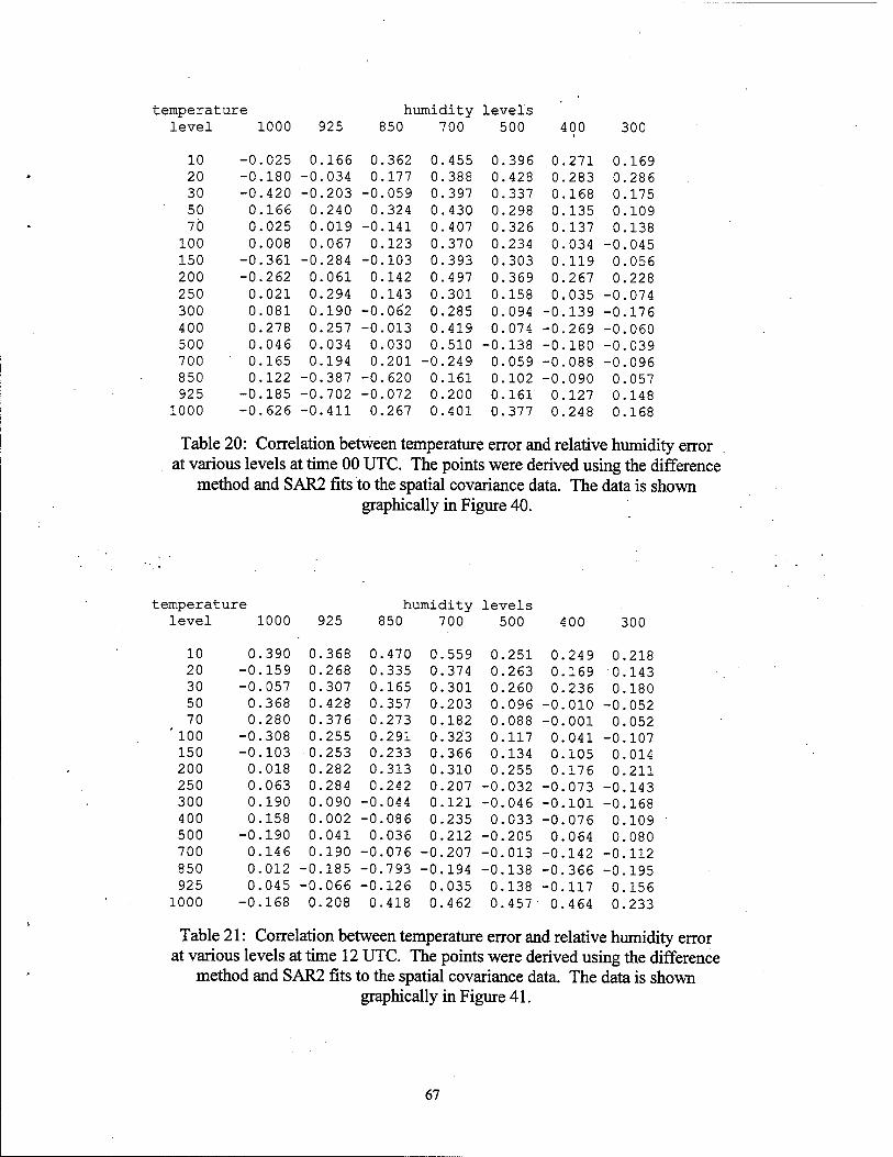
temperature humidity levels level 1000 925 850 700 500 400 300
10 -0.025 0.166 0.362 0.455 0.396 0.271 0.169 20 -0.180 -0.034 0.177 0.388 0.428 0.283 0.286 30 -0.420 -0.203 -0.059 0.397 0.337 0.168 0.175 50 0.166 0.240 0.324 0.430 0.298 0.135 0.109 70 0.025 0.019 -0.141 0.407 0.326 0.137 0.138
100 0.008 0.067 0.123 0.370 0.234 0.034 -0.045 150 -0.361 -0.284 -0.103 0.393 0.303 0.119 0.056 200 -0.262 0.061 0.142 0.4 97 0.369 0.267 0.228 250 0.021 0.294 0.143 0.301 0.158 0.035 -0.074 300 0.081 0.190 -0.0 6'2 0.285 0.094 -0.139 -0.176 400 0.278 0.257 -0.013 0.419 0.074 -0.269 -0.060 500 0.046 0.034 0.030 0.510 -0.138 -0.180 -0.039 700 0.165 0.194 0.201 -0.249 0.059 -0.088 -0.096 850 0.122 -0.387 -0.620 0.161 0.102 -0.090 0.057 925 -0.185 -0.702 -0.072 0.200 0.161 0.127 0.148
1000 -0.626 -0.411 0.267 0.401 0.377 0.248 0.168
Table 20: Correlation between temperature error and relative humidity error at various levels at time 00 UTC. The points were derived using the difference
method and S AR2 fits to the spatial covariance data. The data is shown graphically in Figure 40.
temperati ire humidity levels level 1000 925 850 700 500 400 300
10 0.390 0.368 0.470 0.559 0.251 0.249 0.218 20 -0.159 0.268 0.335 0.374 0.263 0.169 0.143 30 -0.057 0.307 0.165 0.301 0.260 0.236 0.180 50 0.368 0.428 0.357 0.203 0.096 -0.010 -0.052 70 0.280 0.376 0.273 0.182 0.088 -0.001 0.052
' 100 -0.308 0.255 0.291 0.323 0.117 0.041 -0.107 150 -0.103 0.253 0.233 0.366 0.134 0.105 0.014 200 ' 0.018 0.282 0.313 0.310 0.255 0.176 0.211 250 0.063 0.284 0.242 0.207 -0.032 -0.073 -0.143 300 0.190 0.090 -0.044 0.121 -0.046 -0.101 -0.168 400 0.158 0.002 -0.086 0.235 0.033 -0.076 0.109 500 -0.190 0.041 0.036 0.212 -0.205 0.064 0.080 700 0.146 0.190 -0.076 -0.207 -0.013 -0.142 -0.112 850 0.012 -0.185 -0.793 -0.194 -0.138 -0.366 -0.195 925 0.045 -0.066 -0.126 0.035 0.138 -0.117 0.156
1000 -0.168 0.208 0.418 0.462 0.457 ' 0.464 0.233
Table 21: Correlation between temperature error and relative humidity error at various levels at time 12 UTC. The points were derived using the difference
method and SAR2 fits to the spatial covariance data. The data is shown graphically in Figure 41.
67
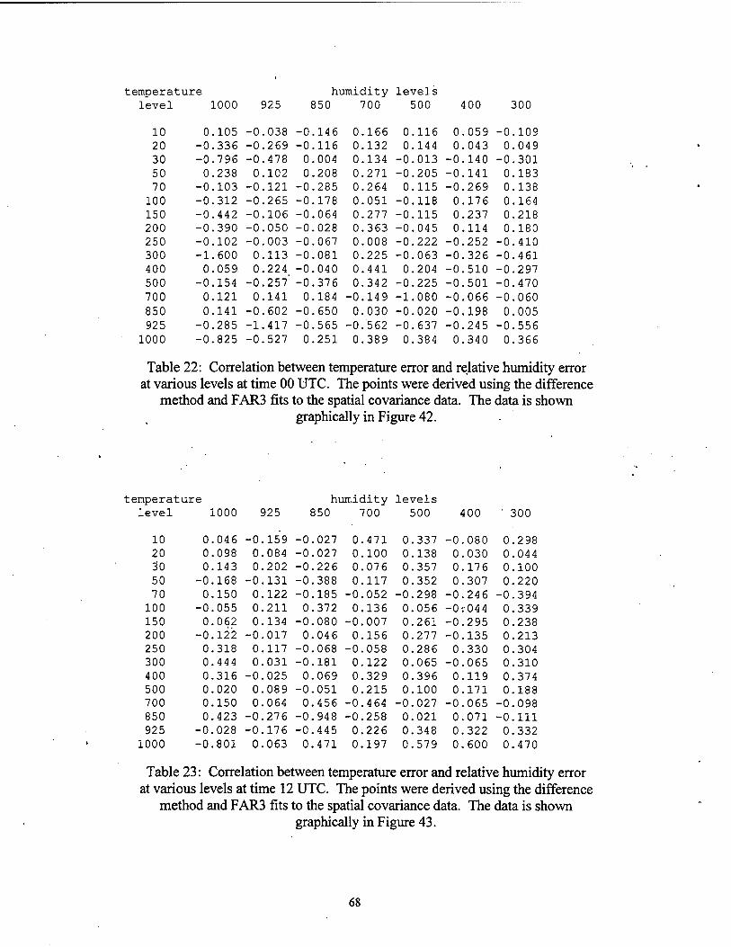
temperature humidity levels level 1000 925 850 700 500 400 300
10 0.105 -0.038 -0.146 0.166 0.116 0.059 -0.109 20 -0.336 -0.269 -0.116 0.132 0.144 0.043 0.049 30 -0.796 -0.478 0.004 0.134 -0.013 -0.140 -0.301 50 0.238 0.102 0.208 0.271 -0.205 -0.141 0.183 70 -0.103 -0.121 -0.285 0.264 0.115 -0.269 0.138 100 -0.312 -0.265 -0.178 0.051 -0.118 0.176 0.164 150 -0.442 -0.106 -0.064 0.277 -0.115 0.237 0.218 200 -0.390 -0.050 -0.028 0.363 -0.045 0.114 0.180 250 -0.102 -0.003 -0.067 0.008 -0.222 -0.252 -0.410 300 -1.600 0.113 -0.081 0.225 -0.063 -0.326 -0.461 400 0.059 0.224 -0.040 0.441 0.204 -0.510 -0.297 500 -0.154 -0.257' -0.376 0.342 -0.225 -0.501 -0.470 700 0.121 0.141 0.184 -0.149 -1.080 -0.066 -0.060 850 0.141 -0.602 -0.650 0.030 -0.020 -0.198 0.005 925 -0.285 -1.417 -0.565 -0.562 -0.637 -0.245 -0.556
1000 -0.825 -0.527 0.251 0.389 0.384 0.340 0.366
Table 22: Correlation between temperature error and relative humidity error at various levels at time 00 UTC. The points were derived using the difference
method and FAR3 fits to the spatial covariance data. The data is shown graphically in Figure 42.
temperati are humidity levels level 1000 925 850 700 500 400 ' 300
10 0.046 -0.159 -0.027 0.471 0.337 -0.080 0.298 20 0.098 0.084 -0.027 0.100 0.138 0.030 0.044 3"0 0.143 0.202 -0.226 0.076 0.357 0.176 0.100 50 -0.168 -0.131 -0.388 0.117 0.352 0.307 0.220 70 0.150 0.122 -0.185 -0.052 -0.298 -0.246 -0.394
100 -0.055 0.211 0.372 0.136 0.056 -0r044 0.339 150 0.062 0.134 -0.080 -0.007 0.261 -0.295 0.238 200 -0.122 -0.017 0.046 0.156 0.277 -0.135 0.213 250 0.318 0.117 -0.068 -0.058 0.286 0.330 0.304 300 0.444 0.031 -0.181 0.122 0.065 -0.065 0.310 400 0.316 -0.025 0.069 0.329 0.396 0.119 0.374 500 0.020 0.089 -0.051 0.215 0.100 0.171 0.188 700 0.150 0.064 0.456 -0.464 -0.027 -0.065 -0.098 850 0.423 -0.276 -0.948 -0.258 0.021 0.071 -0.111 925 -0.028 -0.176 -0.445 0.226 0.348 0.322 0.332
1000 -0.801 0.063 0.471 0.197 0.579 0.600 0.470
Table 23: Correlation between temperature error and relative humidity error at various levels at time 12 UTC. The points were derived using the difference
method and FAR3 fits to the spatial covariance data. The data is shown graphically in Figure 43.
68
References
P. Courtier, E. Andersson, W. Heckley, G. Kelly, J Pailleux, F. Rabier, J.-N.
Thepaut, P. Unden, D. Vasiljevic, C. Cardinali, J. Eyre, M. Hamrud, J. Haseler, A.
Hollingsworth, A. McNally, A. Stoffelen, 1993: Variation Assimilation at ECMWF,
Technical Memorandum No. 194, ECMWF, 84 pp.
Cressie, Noel A. C, 1993: Statistics for Spatial Data, John Wiley & Sons, Inc, 900
pp.
Richard Franke, 1998: Three dimensional covariance functions for NOGAPS data,
submitted to Mon. Wea. Rev. , 37 pp.
Franke, Richard, 1986: Covariance functions for statistical interpolation, TR# NPS-
53-86-007, Naval Postgraduate School, Monterey, CA 93943, 80 pp.
Mitchell, Herschel L., Cecilien Charette, Clement Chouinard, and Bruce Brasnett,
1990: Revised interpolation statistics for the Canadian data assimilation procedure: their
derivation and application, Mon. Weather Rev. 118,1591-1614.
Office of the Federal Coordinator for Meteorological Services and Supporting
Research, Federal Meteorological Handbook No. 3, Rawindsonde and Pibal
Observations, FCM-H3-1997, U. S. Department of Commerce, 1997.
Parrish, D., and J. Derber, 1992: The National Meteorological Center's spectral
statistical interpolation analysis system, Mon. Wea. Rev. 109,1747-1763.
P. Steinle and R. Seaman, 1995: A new 3-D variational analysis scheme, BMRC
Research Report No 54, Bur Met, Australia, pp. 139-144.
69