Vertical Information Sharing in a Volatile Market

Chuan He†1 Johan Marklund‡ Thomas Vossen†

†419 UCB

Leeds School of Business University of Colorado at Boulder

Boulder, CO 80309-0419 Email: chuan.he@colorado.edu

Phone: (303) 492-6658 Fax: (303) 492-5962

‡Department of Industrial Management and Logistics

Lund University P.O. Box 118

SE-22100 Lund Sweden

May 2006

1 Authors are listed in alphabetical order, each author contributed equally. We would like to thank Sven Axsäter, Yongmin Chen, Yuxin Chen, Dmitri Kuksov, Rakesh Niraj, Elie Ofek, Ambar Rao, the area editor and two anonymous reviewers at Marketing Science for their helpful comments. The topic of this paper was inspired by a conversation with Professor Chakravarthi Narasimhan during the first SICS conference in 2003.

Vertical Information Sharing in a Volatile Market

Abstract

When demand is uncertain, manufacturers and retailers often have private information on future

demand, and such information asymmetry impacts strategic interaction in distribution channels. In this

paper, we investigate a channel consisting of a manufacturer and a downstream retailer facing a

product market characterized by short product life, uncertain demand, and price rigidity. Assuming the

firms have asymmetric information about the demand volatility, we examine the potential benefits of

sharing information and contracts that facilitate such cooperation. We conclude that under a wholesale

price regime, information sharing may not improve channel profits when the retailer underestimates

the demand volatility but the manufacturer does not. Although information sharing is always beneficial

under a two-part tariff regime, it is in general not sufficient to achieve information sharing and

additional contractual arrangements are necessary. The contract types we consider to facilitate sharing

are profit sharing and buy back contracts.

Keywords: Channels of Distribution, Decisions under Uncertainty, Game Theory, Supply Chains

1

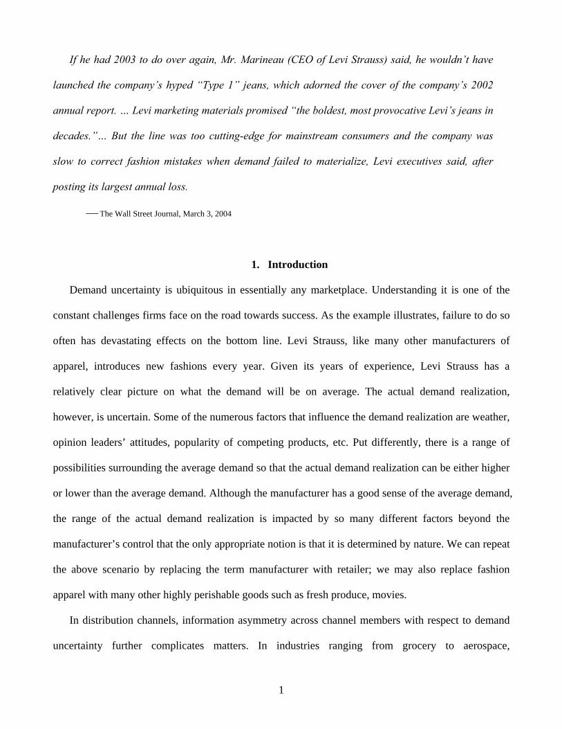
If he had 2003 to do over again, Mr. Marineau (CEO of Levi Strauss) said, he wouldn’t have

launched the company’s hyped “Type 1” jeans, which adorned the cover of the company’s 2002

annual report. … Levi marketing materials promised “the boldest, most provocative Levi’s jeans in

decades.”… But the line was too cutting-edge for mainstream consumers and the company was

slow to correct fashion mistakes when demand failed to materialize, Levi executives said, after

posting its largest annual loss.

⎯ The Wall Street Journal, March 3, 2004

1. Introduction

Demand uncertainty is ubiquitous in essentially any marketplace. Understanding it is one of the

constant challenges firms face on the road towards success. As the example illustrates, failure to do so

often has devastating effects on the bottom line. Levi Strauss, like many other manufacturers of

apparel, introduces new fashions every year. Given its years of experience, Levi Strauss has a

relatively clear picture on what the demand will be on average. The actual demand realization,

however, is uncertain. Some of the numerous factors that influence the demand realization are weather,

opinion leaders’ attitudes, popularity of competing products, etc. Put differently, there is a range of

possibilities surrounding the average demand so that the actual demand realization can be either higher

or lower than the average demand. Although the manufacturer has a good sense of the average demand,

the range of the actual demand realization is impacted by so many different factors beyond the

manufacturer’s control that the only appropriate notion is that it is determined by nature. We can repeat

the above scenario by replacing the term manufacturer with retailer; we may also replace fashion

apparel with many other highly perishable goods such as fresh produce, movies.

In distribution channels, information asymmetry across channel members with respect to demand

uncertainty further complicates matters. In industries ranging from grocery to aerospace,

2

manufacturers and retailers often make independent demand estimates with different degrees of

accuracy. Many factors, such as the proximity to consumers, the availability and quality of customer

databases, sophistication of decision support tools, and experience, contribute to the accuracy of the

demand estimate. Consistent with the opening example, we motivate the core issue of this paper in the

context of a distribution channel of fashion apparel. Before the season begins, the retailer needs to

place an order from the manufacturer. The retailer knows that if she orders too late (say, after the

season begins), she will forgo sales. At this point, the only information available is the demand

estimates (private information) of the manufacturer and the retailer and each party’s profile (public

information). However, neither the manufacturer nor the retailer knows the other party’s estimate

unless it is purposely revealed. Is there any value in sharing the two parties’ demand estimates? If the

answer is positive, what mechanism(s) can help accomplish information sharing?

There is ample evidence that members of a distribution channel can benefit greatly by sharing

demand information. According to an A.T. Kearney report (Field, 2005), the average manufacturer has

enjoyed benefits equivalent to $1 million in savings for every $1 billion of sales by synchronizing their

demand databases with their retailers. However, it is not clear that information sharing is always

feasible in decentralized channels as it is marred by incentive and credibility problems. In the PC

industry, manufacturers often suspect their distributors of submitting “phantom orders”, i.e., forecasts

of high future demand that do not materialize (Zarley and Damore, 1996). Therefore, the value of

information sharing and the mechanisms for facilitating information sharing are topics of great

managerial importance and have received considerable attention in the literature (e.g., Cachon and

Fisher, 2000; Cachon and Lariviere, 2001; Chen, 2003; Gal-Or, 1986; Gu and Chen, 2005; Kulp, Lee

and Ofek, 2004; Lee, Padmanabhan and Whang, 1997; Lee, So and Tang, 2000; Li, 2002; Niraj and

Narasimhan, 2002; Villas-Boas, 1994; Vives, 1984).

In this paper, we focus on a product market characterized by short product life, uncertain demand,

and price rigidity (lack of price promotion). A catalogue marketer of fashion goods is a prototypical

3

example of such a market. Due to the inherent uncertainty about consumer tastes, fashion goods are

synonymous with rapid change and subject to significant demand variability. We investigate a

distribution channel with one manufacturer and one retailer, each with private information about the

distribution of future demand. Our objective is to examine the benefits of sharing information about

future demand volatility and contracts that facilitate such cooperation. More precisely, we consider

multiplicative demand uncertainty, uniformly distributed between an upper and a lower bound about

which the members of the channel have asymmetric information. To capture the impact of uncertainty,

we model the retailer as a newsvendor problem with endogenous pricing. This allows us to balance the

expected cost of ordering too much with the expected opportunity cost of ordering too little, when

maximizing the retailer profits. The manufacturer is assumed to operate under a constant marginal cost,

without any capacity constraints.

Several notable features emerge from our model setup. First, the environment under consideration

is a one-shot, highly volatile setting; firms engage in short-term relationships and cannot refine their

demand estimates by using historical data. Second, firms’ demand estimates may either overshoot or

undershoot the true demand volatility because the demand is intrinsically stochastic, and the

correlation between the firms’ demand estimates is unknown. Thus, there is no obvious way to

combine or pool them into a more accurate estimate.

We find that sharing information about market demand volatility does not always improve channel

profits. In particular, under a wholesale price only regime, when the retailer underestimates the

demand variability but the manufacturer does not, sharing can lead to lower channel profits. In addition,

we show that the feasibility of information sharing not only depends on the asymmetric estimates of

the demand volatility but also on the channel members’ knowledge of the quality of each member’s

forecast. Specifically, we demonstrate that a profit sharing contract is a viable mechanism when each

channel member is aware of the quality of the other member’s demand forecast relative to its own,

4

whereas buy back contracts can improve channel coordination when only one member knows whose

demand forecast is more accurate.

We also find that under a two-part tariff regime, sharing information about market demand

volatility always improves channel profits, but additional contractual arrangements are needed for

sharing to occur. In contrast to the symmetric case, under asymmetric information about demand

volatility, a two-part tariff does not always coordinate the channel.

Three streams of literature are relevant to our study: the literature on channel coordination, the

literature on newsvendor models with endogenous pricing decisions, and the emerging literature on

information sharing. The extant channel literature generally assumes deterministic demand (e.g.,

Jeuland and Shugan, 1983; McGuire and Staelin, 1983). The limited channel literature that

incorporates demand uncertainty usually assumes that uncertainty is a white noise and has no

consequence as firms maximize expected profits (e.g., Lal, 1990), or models uncertainty as consisting

of a high state and a low state (e.g., Biyalogorsky and Koenigsberg, 2004; Desai, 2000; Padmanabhan

and Png, 1997; Gu and Chen, 2005). These papers primarily consider the impact of uncertainty in the

demand trend (i.e., the mean), but do not focus on the impact of asymmetric information about demand

volatility. Such treatment allows researchers to obtain a high level of parsimony, which facilitates the

analysis of complex issues such as channel structure, upstream/downstream competition, multi-period

interaction, etc. However, this parsimony is obtained at the cost of generality. In particular, the actual

demand realization may be either above or below the demand trend and firms incur costs in either case.

By focusing on demand trend but ignoring volatility, one assumes that the costs associated with

undershooting and overshooting are identical (we shall revisit this point in details in Section 3.3). This

assumption becomes very troublesome when demand volatility is large, as in the case of highly

perishable goods. We complement this literature by looking at demand uncertainty from a different

perspective, focusing on the impact of asymmetric estimates of the demand volatility in a newsvendor

setting with uniformly distributed demand uncertainty.

5

The classical newsvendor approach offers an intuitive way to incorporate the effect of demand

volatility into the analysis of channel behavior. In a one-period setting, the retailer (newsvendor) trades

off the marginal cost of understocking with that of overstocking when determining how much to order.

In its traditional formulation, the newsvendor model determines the quantity to order under the

assumption that price is an exogenously set parameter which does not affect demand (See Porteus

(1990) for a comprehensive review of general newsvendor problems). The impact of adding pricing

decisions to the newsvendor problem was first considered by Whitin (1955). Mills (1959) considers

this problem under the assumption of additive demand uncertainty, while Karlin and Carr (1962)

assume multiplicative demand uncertainty. For a comprehensive review of the newsvendor problem

with endogenous pricing we refer to Petruzzi and Dada (1999), who propose a unified view of the

above mentioned approaches.

Demand uncertainty and the use of local demand information often lead to severe distortion and

loss of channel profits. A related issue is the inherent amplification of demand variability as local

demand information is transmitted along a distribution channel. The phenomenon, which is due to

successive distortion of the demand information, is often referred to as the “bullwhip effect.” It was

first illustrated in Forrester (1958) and more recently analyzed by Lee, Padmanabhan and Whang

(1997), the latter spawning a large number of publications on this issue, for which one remedy is

information sharing.

Lee, So and Tang (2000) study information sharing in supply chains with long-term relationships

and find that the value of information sharing is high when the demand correlation over time is high

and when the demand variance within each time period is high. However, information sharing is

complicated by incentive and credibility problems that arise from information asymmetry. Cachon and

Lariviere (2001) explore capacity decisions in a supply chain with one manufacturer and one supplier

(retailer). They show that the use of forcing contracts (involuntary compliance) vs. self-enforcing

contracts (voluntary compliance) significantly impacts the outcome of demand forecast sharing. Li

6

(2002) examines the incentives for firms to share information vertically in a supply chain with one

manufacturer and many retailers. He shows that voluntary information sharing is often infeasible when

the retailers are engaged in a Cournot competition and are endowed with some private information. For

excellent reviews of information sharing and contracts in supply chain coordination, readers are

referred to Cachon (2003) and Chen (2003).

Our paper differs from the above mentioned literature in two aspects. First, we study the value of

information sharing in a distribution channel in which the members have asymmetric information

about demand volatility. Second, we examine the mechanisms for facilitating information sharing in

the context of short-term relationships, where cooperative behavior is rare and forcing contracts of any

kind are difficult to implement.

The remainder of the paper is organized as follows. Section 2 lays out the key elements of the

model. Section 3 analyzes the basic model, in which a manufacturer and a retailer with asymmetric

information about demand volatility operate under a wholesale price only regime without information

sharing. Section 4 explores the value of sharing this type of information, and how to facilitate sharing

using different contractual agreements. Section 5 considers the impact of sharing information under a

two-part tariff regime instead of a wholesale price mechanism. Section 6 concludes.

2. Assumptions and model set-up

The distribution channel we consider consists of a manufacturer and a downstream retailer; both

firms are risk neutral and maximize their expected profits. Given that p represents the retail price, end-

customer demand is given by ,)()( εpypD = where bappy −=)( (defined for 0, 1a b> > ) is a price

dependent deterministic function, and ε is a uniformly distributed random variable with mean of 1.

More precisely, ε ∈U[1−L,1+L] for 10 ≤≤ L , with (.)f and (.)F denoting its pdf and cdf. Hence, end-

customer demand is determined by a random draw from the distribution U[1–L,1+L], where nature

7

determines the extent of uncertainty L. The demand is intrinsically stochastic with an average of )( py ,

a standard deviation of 3L)p(y , and a volatility which decreases (increases) as L tends to 0 (1). It

follows that the average demand )( py tends to 0 as p grows very large, and goes to infinity as p

approaches 0. This property is innocuous and is equivalent to the usual assumption that the demand

reaches the market potential (usually a constant) when the product is free. The parameter b measures

price sensitivity. We assume that the price elasticity of the average demand b is common knowledge

and that b > 1 so that the demand is sufficiently elastic.

In our model, the random variable ε captures demand uncertainty, the functional form of its

distribution (uniform) and its mean are common knowledge. The only unknown is the variance of ε,

which is characterized by the lower and upper bounds of the distribution 1−L and 1+L. As such, the

manufacturer and the retailer need to form estimates of L independently.

The steps in our model are as follows. First, the manufacturer determines the wholesale price w,

using its private demand estimate, εm, to predict the retailer’s reaction. We assume that the

manufacturer has a constant marginal cost, c, unknown to the retailer, and does not have any capacity

constraints. (The assumption that c is private information is motivated by the fact that the marginal

costs are highly dependent upon the manufacturer’s organizational capabilities, which in general are

unknown to the retailer.) Subsequently, the retailer, with the wholesale price w at hand, sets the retail

price, p, and places an order, q, using its own demand estimate εr. Finally, the demand D(p) is realized.

If ( )D p q> , the retailer experiences a shortage and incurs an opportunity cost in terms of profits lost,

( )( )p w D p q− −⎡ ⎤⎣ ⎦ ; if ( )D p q< , the retailer has leftover products over which it incurs a loss,

( )w q D p−⎡ ⎤⎣ ⎦ . We assume that neither the retailer nor the manufacturer incurs any goodwill cost in the

event of shortage, and that any leftover products have zero salvage value. However, it would be

possible to extend our model to incorporate these.

8

The resulting framework can be viewed as a one-period game of incomplete information, and the

appropriate solution concept in this setting would be the Bayesian-Nash equilibrium. Specifically, the

firms’ optimal strategies need to be consistent with their beliefs derived from Bayes rule. In our

framework, however, the beliefs do not impact our results. This is because (i) as we will show in

Section 3.2, the optimal wholesale price w is independent of Lm and does not convey any useful

information about the manufacturer’s estimate to the retailer, and (ii) even though the manufacturer

may deduce the retailer estimate Lr, this has no consequence on the optimal wholesale price, and the

equilibrium solution remains unchanged. Therefore, it is rational for a firm to use its own estimate.

Formally, the non-Bayesian nature of the game is illustrated by the following claims:

Claim 1: The manufacturer and the retailer form point estimates of L.

Proof: All proofs are in the Appendix.

Claim 2: The manufacturer’s wholesale price w is uninformative.

Claim 3: Without information sharing ( mL is unknown to the retailer), it is rational for the retailer

to use her own estimate rL ; with information sharing, a known mL triggers an all-or-nothing

update.

Now suppose that the manufacturer and the retailer each form a point estimate of L, their beliefs on

ε are then given by [ ]1 , 1m m mU L Lε ∈ − + and [ ]1 , 1r r rU L Lε ∈ − + , respectively. Note that it is

possible that iL L≤ or iL L≥ , where i = r,m. In words, the manufacturer and the retailer can either

overestimate or underestimate L. Since the mean of the demand distribution is known, a firm’s demand

estimate is superior if its estimated variance is closer to the true state. According to our definition, iL is

superior to jL if i jL L L L− < − . At the same time, the manufacturer and the retailer each receive a

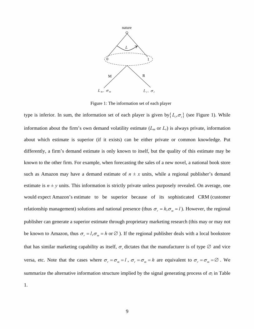
signal iσ that reveals the type of the other player. For simplicity, we assume that each player can be of

three types{ }, ,h l∅ , where h type is superior, ∅ type is the same as the other player or unknown, l

9

nature

L

0 1

M R

L m , σ m L r , σ r

Figure 1: The information set of each player

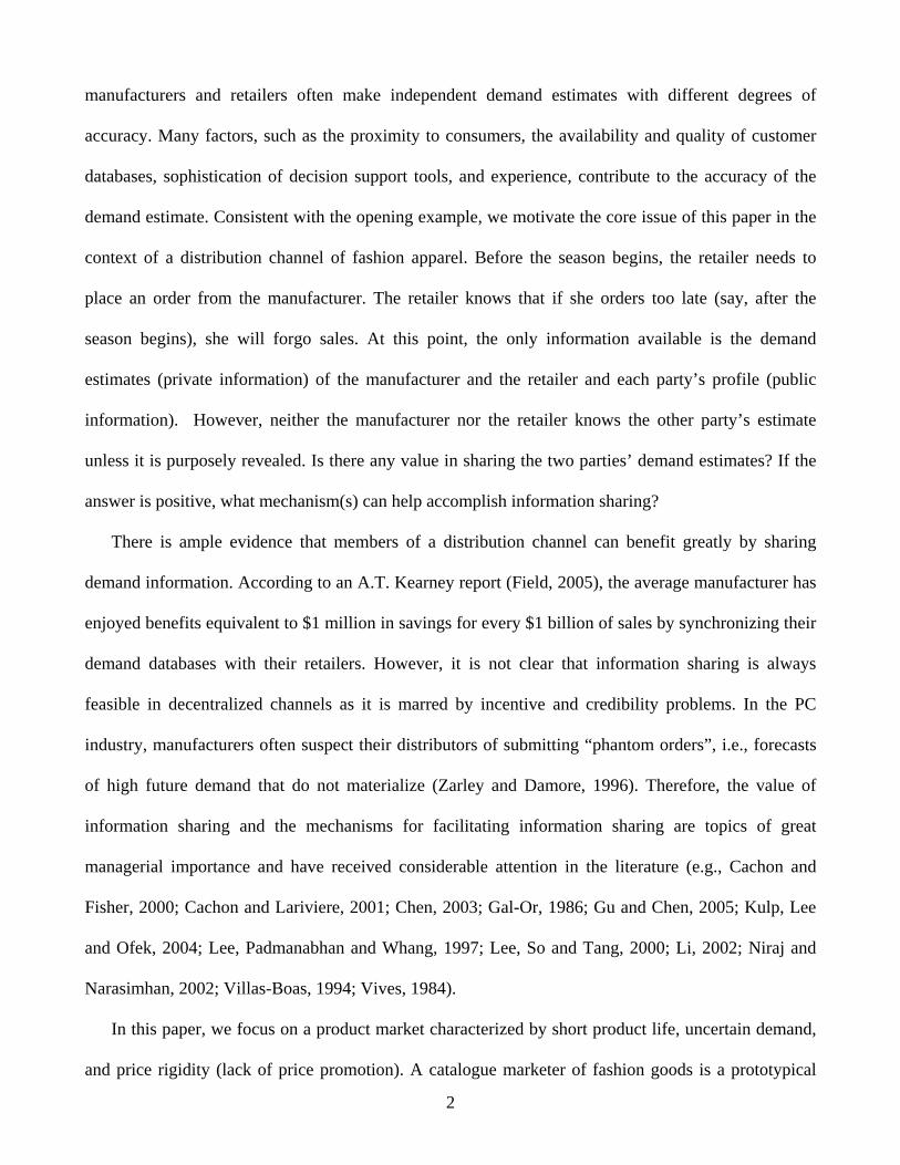
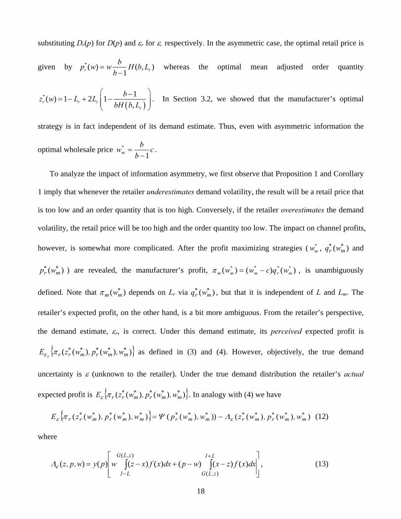
type is inferior. In sum, the information set of each player is given by{ },i iL σ (see Figure 1). While

information about the firm’s own demand volatility estimate (Lm or Lr) is always private, information

about which estimate is superior (if it exists) can be either private or common knowledge. Put

differently, a firm’s demand estimate is only known to itself, but the quality of this estimate may be

known to the other firm. For example, when forecasting the sales of a new novel, a national book store

such as Amazon may have a demand estimate of n ± x units, while a regional publisher’s demand

estimate is n ± y units. This information is strictly private unless purposely revealed. On average, one

would expect Amazon’s estimate to be superior because of its sophisticated CRM (customer

relationship management) solutions and national presence (thus ,r mh lσ σ= = ). However, the regional

publisher can generate a superior estimate through proprietary marketing research (this may or may not

be known to Amazon, thus , or r ml hσ σ= = ∅ ). If the regional publisher deals with a local bookstore

that has similar marketing capability as itself, rσ dictates that the manufacturer is of type ∅ and vice

versa, etc. Note that the cases where r m lσ σ= = , r m hσ σ= = are equivalent to r mσ σ= =∅ . We

summarize the alternative information structure implied by the signal generating process of σi in Table

1.

10

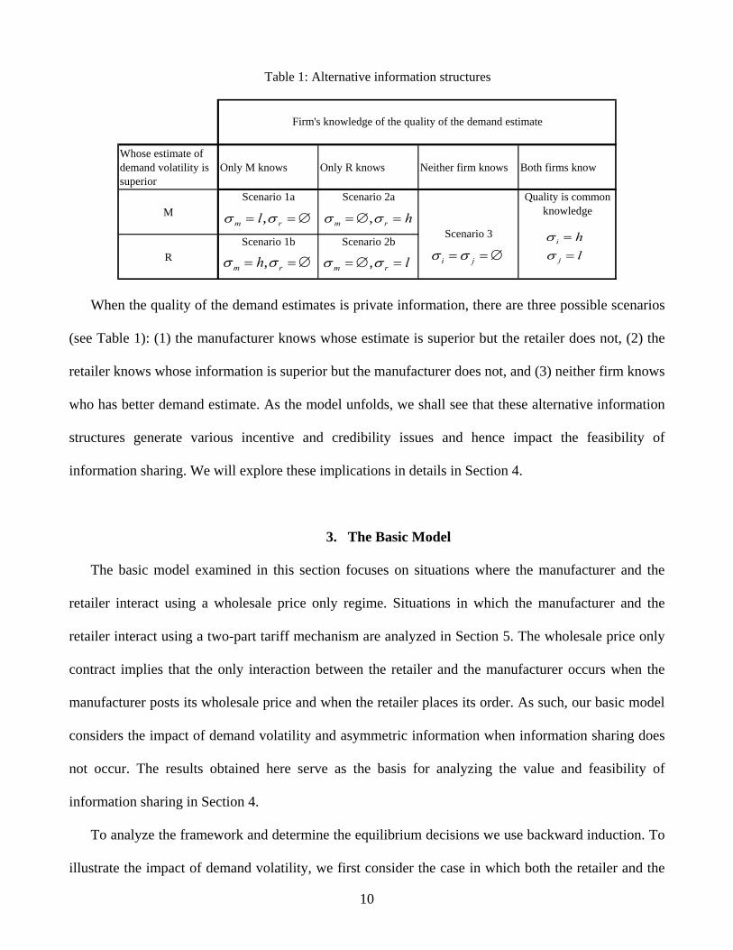
Table 1: Alternative information structures

Whose estimate of demand volatility is superior

Only M knows Only R knows Neither firm knows Both firms know

MScenario 1a Scenario 2a

RScenario 1b Scenario 2b

Scenario 3

Firm's knowledge of the quality of the demand estimate

Quality is common knowledge

i jσ σ= = ∅i

j

hl

σσ

=

=,m rhσ σ= = ∅

,m rlσ σ= = ∅ ,m r hσ σ= ∅ =

,m r lσ σ= ∅ =

When the quality of the demand estimates is private information, there are three possible scenarios

(see Table 1): (1) the manufacturer knows whose estimate is superior but the retailer does not, (2) the

retailer knows whose information is superior but the manufacturer does not, and (3) neither firm knows

who has better demand estimate. As the model unfolds, we shall see that these alternative information

structures generate various incentive and credibility issues and hence impact the feasibility of

information sharing. We will explore these implications in details in Section 4.

3. The Basic Model

The basic model examined in this section focuses on situations where the manufacturer and the

retailer interact using a wholesale price only regime. Situations in which the manufacturer and the

retailer interact using a two-part tariff mechanism are analyzed in Section 5. The wholesale price only

contract implies that the only interaction between the retailer and the manufacturer occurs when the

manufacturer posts its wholesale price and when the retailer places its order. As such, our basic model

considers the impact of demand volatility and asymmetric information when information sharing does

not occur. The results obtained here serve as the basis for analyzing the value and feasibility of

information sharing in Section 4.

To analyze the framework and determine the equilibrium decisions we use backward induction. To

illustrate the impact of demand volatility, we first consider the case in which both the retailer and the

11

manufacturer have symmetric and accurate information, that is, r mL L L= = . Section 3.1 derives the

retailer’s profit maximizing strategy for this case, given the wholesale price determined by the

manufacturer. Based on these results, the manufacturer’s decision problem is analyzed in Section 3.2.

Subsequently, section 3.3 provides insights as to the impact of demand volatility on the equilibrium

strategies. Finally, section 3.4 discusses the impact of information asymmetry on the equilibrium

strategies. Although Sections 3.1 and 3.2 are integral components of our analysis, they focus on the

technical aspects of the model and are relatively self-contained. Readers who are not interested in the

underlying mathematics of the model development can go directly to Sections 3.3 and 3.4 to obtain the

key insights from the model.

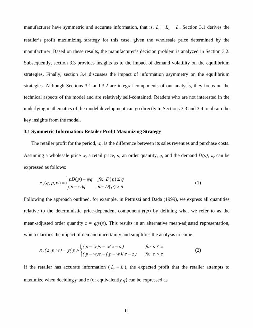
3.1 Symmetric Information: Retailer Profit Maximizing Strategy

The retailer profit for the period, πr, is the difference between its sales revenues and purchase costs.

Assuming a wholesale price w, a retail price, p, an order quantity, q, and the demand D(p), πr can be

expressed as follows:

⎩⎨⎧

>−≤−

=qpDforqwpqpDforwqppD

wpqr )()()()(

),,(π (1)

Following the approach outlined, for example, in Petruzzi and Dada (1999), we express all quantities

relative to the deterministic price-dependent component )( py by defining what we refer to as the

mean-adjusted order quantity z = q/y(p). This results in an alternative mean-adjusted representation,

which clarifies the impact of demand uncertainty and simplifies the analysis to come.

⎩⎨⎧

>−−−−≤−−−

⋅=zfor)z)(wp()wp(zfor)z(w)wp(

)p(y)w,p,z(r εεεεεε

π (2)

If the retailer has accurate information ( rL L= ), the expected profit that the retailer attempts to

maximize when deciding p and z (or equivalently q) can be expressed as

12

{ }1

1

1

1

( , , ) ( ) ( ) ( )

( ) ( ) ( ) ( ) ( )

L

rL

z L

L z

E z p w y p p w xf x dx

w z x f x dx p w x z f x dx

ε π+

−

+

−

⎡= −⎢

⎣⎤

− − − − − ⎥⎦

∫

∫ ∫ (3)

Defining

)wp)(p(y)w,p( −=Ψ and

1

1

2

( , , ) ( ) ( ) ( ) ( ) ( ) ( )

( ) ( ) ( )(1 )

z L

L z

z p w y p w z x f x dx p w x z f x dx

y p LpF z p w z

ε

+

−

⎡ ⎤Λ = − + − −⎢ ⎥

⎣ ⎦⎡ ⎤= + − −⎣ ⎦

∫ ∫

we can also write

{ }( , , ) ( , ) ( , , )rE z p w p w z p wε επ = Ψ −Λ . (4)

Hence, the expected profit can be expressed as the riskless profit, Ψ(p,w), which represents the profit

obtained by the retailer in the deterministic problem (e.g. 0L = ), less the expected loss that results

from the presence of uncertainty, expressed by the loss function ( , , )z p wεΛ . Note that the expected

loss equals the sum of the expected cost of ordering too much and the expected opportunity cost of

ordering too little.

To determine the optimal price )w(p*r and mean-adjusted order quantity )w(z*

r that maximize (3)

and (4) for a given w, we consider the first-order optimality conditions and proceed by taking the first

partial derivatives of { }( , , )rE z p wε π with respect to z and p:

{ } [ ]( , , ) ( , , ) ( ) ( ) ( )rE z p w z p w y p p w pF zz z

ε επ∂ ∂Λ= − = − −

∂ ∂

{ } 2( , , )( ) (1 ) ( 1) ( )rE z p w p wy p z b b LF z

p pε π∂ ⎡ ⎤−

= − + −⎢ ⎥∂ ⎣ ⎦

Observe that for any given p the optimal mean-adjusted order quantity )w,p(z*r corresponds to the

standard newsvendor result, that is,

13

* 1( , ) ( ) 1 2rp w p wz p w F L L

p p− − −

= = − + . (5)

It is easy to see from (5) that )w,p(z*r is increasing in p. Intuitively, the explanation for this is that the

opportunity cost for every unsatisfied demand (p − w) increases with p, while the cost of every surplus

item remains constant at w.

Similarly, for any given z we can determine the optimal price *( , )rp z w :

*2( , )

1 ( )b zp z w w

b z LF z⎡ ⎤⎛ ⎞= ⎜ ⎟ ⎢ ⎥− −⎝ ⎠ ⎣ ⎦

(6)

Observe that whenever demand is deterministic (e.g. 0L = ), the optimal riskless price 1b

bw)w(p*r −

= .

Moreover, we note that 2 ( )z LF z z− < since both L and ( )F z are non-negative, and that

2 ( ) 0z LF z− > since 1L ≤ and 2 ( ) ( )F z F z z≤ ≤ . Thus, equation (6) illustrates the well-known result

(Karlin and Carr, 1962) that the introduction of uncertainty will yield a price that is larger than the

optimal riskless price, i.e. 1b

bw)w(p*r −

≥ .

Using (5) (or (6)), the retailer’s profit maximization problem can be reduced to an optimization

problem over a single variable. Substituting the expression for *( , )rz p w into the expected profit

function (4) renders the expression

{ }*( ( , ), , ) ( ) ( ) 1r rwE z p w p w y p p w Lpε π

⎡ ⎤⎛ ⎞= − −⎢ ⎥⎜ ⎟

⎝ ⎠⎣ ⎦,

which is decreasing in the demand volatility L. Using the first order optimality condition with respect

to p, renders )w(p*r as specified in Lemma 1.

Lemma 1: For any given w, the optimal retail price

*( ) ( , )1r

bp w w H b Lb

=−

, (7)

14

where

2

2

1 1( , ) 12 2

L L LH b Lb

+ −⎛ ⎞= + + >⎜ ⎟⎝ ⎠

. (8)

Note that [b/(b− 1)]H(b,L) can be viewed as a generalized double marginalization factor, which is

minimized for the special case of deterministic demand (i.e., L = 0) where it degenerates to b/(b-1).

From Lemma 1 it is easy to determine the optimal mean adjusted order quantity )w(z*r by substituting

)w(p*r for p in (5).

( ) ( )* 1 1 1( ) 1 1 2 1

, ,rb bz w F L L

bH b L bH b L− ⎛ ⎞ ⎛ ⎞− −

= − = − + −⎜ ⎟ ⎜ ⎟⎜ ⎟ ⎜ ⎟⎝ ⎠ ⎝ ⎠

(9)

The corresponding actual order quantity, )w(q*r , follows directly as ))w(p(y)w(z)w(q *

r*r

*r = .

3.2 Symmetric Information: Manufacturer Profit Maximizing Strategy

The manufacturer has to determine an optimal wholesale price *mw . Given that, in the current case,

the retailer and manufacturer have symmetric and accurate information, the manufacturer can predict

the retailer’s response to any given order quantity he chooses. Consequently, the retailer’s profit

function, as a function of the wholesale price, can be expressed as

* *( ) ( ) ( ( ), )

1 1( ) 1 2 ( , ) ( )( , ) 1

m r rb

w w c q p w w

b bw c L L H b L y wb H b L b

π−

= −

⎛ ⎞− ⎛ ⎞= − + −⎜ ⎟⎜ ⎟−⎝ ⎠⎝ ⎠

(10)

Note that πm(w) is a deterministic function, that is, the manufacturer’s profit is determined by how

much the retailer orders instead of actual sales during the period. This implies that the manufacturer

does not expose itself to any risk associated with demand uncertainty. To determine the manufacturer’s

optimal wholesale price *mw , we use the first order optimality condition for πm(w) with respect to w,

( )( ) 11 1 2 ( , ) 0( , ) 1

bm w w c b bb L L H b L y ww w bH b L b

π −⎛ ⎞∂ − −⎛ ⎞ ⎛ ⎞= − + − =⎜ ⎟⎜ ⎟ ⎜ ⎟∂ −⎝ ⎠ ⎝ ⎠⎝ ⎠.

15

Solving for w yields

cb

bwm 1*

−= , (11)

It is interesting to note that *mw is in fact independent of the demand volatility L, and worth pointing

out that this is unlikely to hold if the manufacturer faces constrained capacity, which typically creates a

complex relationship between c and the quantity ordered. Finally, we also note that in the case of

deterministic demand (L = 0), (11) together with (6) illustrates the well-known double-marginalization

principle.

3.3 Impact of Demand Volatility

From the above, we conclude that for given estimates of the demand volatility L, the profit

maximizing strategy for the manufacturer is to set a wholesale price *mw and the optimal response for

the retailer is to order )w(q *m

*r units which are sold at a retail price of )w(p *

m*r . To analyze the value

of information sharing, an important question is how changes in the demand volatility estimates impact

these decisions and the associated profits. In the remainder of this section we provide some structural

properties that help answer these questions. First, however, we observe that since the manufacturer’s

optimal wholesale price *mw is independent of L (see (11)), the profit maximizing strategies are

unaffected by changes in the manufacturer’s estimate of the demand volatility. We therefore

concentrate on the impact of demand volatility changes on the retailer’s strategy.

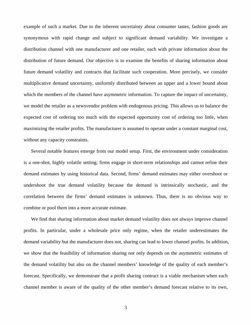
In the presence of demand volatility, the order quantity ( )*rq w generally differs from the average

demand *( ( ))ry p w due to the asymmetry between the costs associated with understocking and

overstocking.

Lemma 2: For any given L , ( )* *( ( ))r rq w y p w> if and only if 1( , ) 2 bH b Lb−⎛ ⎞> ⎜ ⎟

⎝ ⎠ .

16

L0 1

z

1

L0 1

*q

( )*y p

z

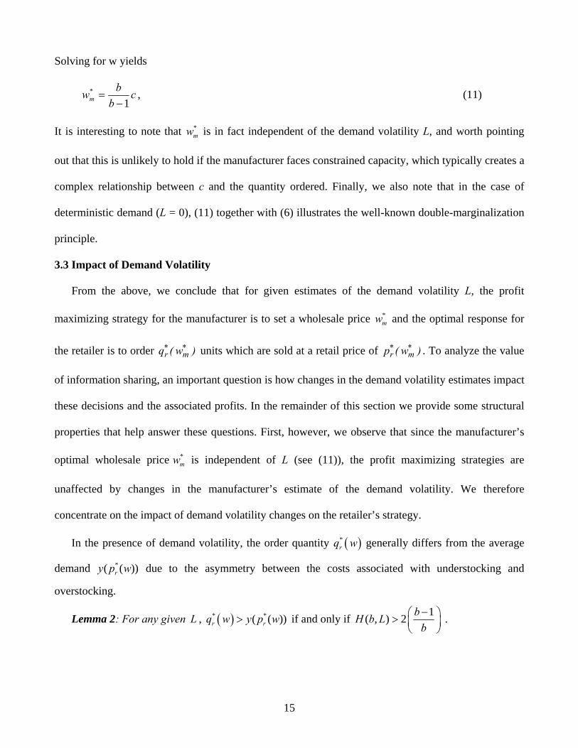
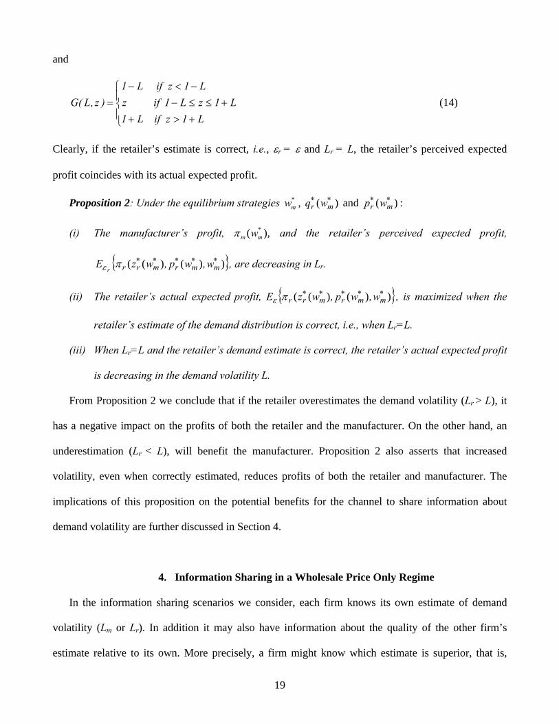
Figure 2: Impact of demand volatility on order quantity.

This is illustrated in Figure 2, which shows both the mean-adjusted and the absolute order quantity as a

function of L . Clearly, ( )* *( ( ))r rq w y p w= when 0L = . However, as L increases *( )z w will initially

decrease below 1 (and therefore ( )* *( ( ))r rq w y p w< ), until we reach the value of L for which

1( , ) 2 bH b Lb−⎛ ⎞= ⎜ ⎟

⎝ ⎠. For larger values of L , *( )z w will be larger than 1.

In addition, the retailer can fine-tune the costs of overstocking and understocking since it has the

ability to set prices, which will cause the retail price *( )rp w to differ from the optimal riskless price

1bbw)w(p*

r −= . As discussed in the introduction of this paper, the conventional approach to demand

uncertainty focuses on the mean, but fails to account for these additional trade-offs that are caused by

the introduction of demand volatility. This may become problematic when demand volatility is an

important factor. We note that while a two-point distribution can also account for the effect of demand

volatility, it is impossible to disentangle the effect of the mean from that of variance in such

distributions, since any change in the variance will also imply a change in the mean.

To illustrate the impact of demand volatility, we first consider its impact on the optimal retail price.

Proposition 1: The profit maximizing retail price *( )rp w is strictly increasing in L .

17

Intuitively, by increasing the retail price, the retailer can reduce the demand variability (recall that

its standard deviation is 3L)p(y and that y(p) is decreasing in p) and counter the effect of an

increase in L on the loss term ( , , )z p wεΛ . Of course, an increase in the retail price also reduces the

mean demand, y(p), which implies a reduction in the riskless profit ( , )p wΨ .

To illustrate how demand volatility impacts the optimal order quantity *( )rq w we first observe that,

while the mean-adjusted order quantity )w,p(z*r is increasing in p, the actual order quantity

)w,p(z)p(y)w,p(q *r

*r = will have a maximum. Intuitively, this follows since any increase in

)w,p(z*r are countered by a decrease in the mean demand )( py = ap-b as p increases.

Lemma 3: For any given w, )w,p(q*r strictly increases with respect to p when

21 1

b Lp wb L

⎛ ⎞⎛ ⎞≤ ⎜ ⎟⎜ ⎟+ +⎝ ⎠⎝ ⎠ and strictly decreases with respect to p when 2

1 1b Lp w

b L⎛ ⎞⎛ ⎞≥ ⎜ ⎟⎜ ⎟+ +⎝ ⎠⎝ ⎠

.

Corollary 1: The profit maximizing order quantity *( )rq w is strictly decreasing in L .

Observe that corollary 1 immediately follows from Proposition 1 and Lemma 3, since

* 2( )1 1 1

b b Lp w w wb b L

⎛ ⎞⎛ ⎞≥ > ⎜ ⎟⎜ ⎟− + +⎝ ⎠⎝ ⎠.

3.4 Impact of Information Asymmetry

Let us now consider the situation where the retailer and the manufacturer have asymmetric demand

estimates, which may both be different from the true demand volatility L. Thus, the retailer’s estimate

Lr may be different from the manufacturer’s estimate Lm.

In this case, the basic model is again derived from backward induction. However, when the retailer

makes its decisions regarding retail price and order quantity to maximize its expected profits (given w),

it does so ex ante without knowing D(p). Instead, it has to rely on its best demand estimate Dr(p). The

associated profit function, and consequently the expected profit, are equivalent to (2) and (3) after

18

substituting Dr(p) for D(p) and εr for ε, respectively. In the asymmetric case, the optimal retail price is

given by *( ) ( , )1r r

bp w w H b Lb

=−

whereas the optimal mean adjusted order quantity

( )* 1( ) 1 2 1

,r r rr

bz w L LbH b L

⎛ ⎞−= − + −⎜ ⎟⎜ ⎟

⎝ ⎠. In Section 3.2, we showed that the manufacturer’s optimal

strategy is in fact independent of its demand estimate. Thus, even with asymmetric information the

optimal wholesale price cb

bwm 1*

−= .

To analyze the impact of information asymmetry, we first observe that Proposition 1 and Corollary

1 imply that whenever the retailer underestimates demand volatility, the result will be a retail price that

is too low and an order quantity that is too high. Conversely, if the retailer overestimates the demand

volatility, the retail price will be too high and the order quantity too low. The impact on channel profits,

however, is somewhat more complicated. After the profit maximizing strategies ( *mw , )( *

m*r wq and

)( *m

*r wp ) are revealed, the manufacturer’s profit, )()()( ***

mr*mmm wqcww −=π , is unambiguously

defined. Note that )( *mm wπ depends on Lr via )( *

m*r wq , but that it is independent of L and Lm. The

retailer’s expected profit, on the other hand, is a bit more ambiguous. From the retailer’s perspective,

the demand estimate, εr, is correct. Under this demand estimate, its perceived expected profit is

{ }))()(( *m

*m

*r

*m

*rr w,wp,wzE

rπε as defined in (3) and (4). However, objectively, the true demand

uncertainty is ε (unknown to the retailer). Under the true demand distribution the retailer’s actual

expected profit is { }))()(( *m

*m

*r

*m

*rr w,wp,wzE πε . In analogy with (4) we have

{ } ))()(()))(())()(( *m

*m

*r

*m

*r

*m

*m

*r

*m

*m

*r

*m

*rr w,wp,wzw,wpw,wp,wzE εε ΛΨπ −= (12)

where

⎥⎥⎦

⎤

⎢⎢⎣

⎡−−+−= ∫∫

+

−

L1

z,LG

z,LG

L1dxxfzxwpdxxfxzwpyw,p,z

)(

)()()()()()()()(εΛ , (13)

19

and

⎪⎩

⎪⎨

⎧

+>++≤≤−

−<−=

L1zifL1L1zL1ifz

L1zifL1)z,L(G (14)

Clearly, if the retailer’s estimate is correct, i.e., εr = ε and Lr = L, the retailer’s perceived expected

profit coincides with its actual expected profit.

Proposition 2: Under the equilibrium strategies *mw , )( *

m*r wq and )( *

m*r wp :

(i) The manufacturer’s profit, ),( *mm wπ and the retailer’s perceived expected profit,

{ }))()(( *m

*m

*r

*m

*rr w,wp,wzE

rπε , are decreasing in Lr.

(ii) The retailer’s actual expected profit, { }))()(( *m

*m

*r

*m

*rr w,wp,wzE πε , is maximized when the

retailer’s estimate of the demand distribution is correct, i.e., when Lr=L.

(iii) When Lr=L and the retailer’s demand estimate is correct, the retailer’s actual expected profit

is decreasing in the demand volatility L.

From Proposition 2 we conclude that if the retailer overestimates the demand volatility (Lr > L), it

has a negative impact on the profits of both the retailer and the manufacturer. On the other hand, an

underestimation (Lr < L), will benefit the manufacturer. Proposition 2 also asserts that increased

volatility, even when correctly estimated, reduces profits of both the retailer and manufacturer. The

implications of this proposition on the potential benefits for the channel to share information about

demand volatility are further discussed in Section 4.

4. Information Sharing in a Wholesale Price Only Regime

In the information sharing scenarios we consider, each firm knows its own estimate of demand

volatility (Lm or Lr). In addition it may also have information about the quality of the other firm’s

estimate relative to its own. More precisely, a firm might know which estimate is superior, that is,

20

whether Lm or Lr is closer to the true state L. However, as discussed in Section 2, L as well as the

correlation between the estimates are unknown. Under this information asymmetry, the firm with a

superior estimate needs a mechanism to convey its information (about Lm or Lr) to the other firm when

it is profitable to do so. The transmission of this information can only be successful if the other firm

finds itself better off, or at least no worse off, to use such information. Throughout this paper, we say

that information sharing occurs when such transmission is successful, that is, when the firms share

their private information about demand volatility (Lm or Lr). An important observation explained in

Sections 2 is that belief updating is moot for the situation we consider.

To better understand the incentive and credibility problems in information sharing, we outline the

taxonomy of alternative information structures, summarized in Table 1 (on p. 10). We discuss each of

these scenarios in turn.

In Scenario 1, if the manufacturer’s estimate is superior (Scenario 1a), he needs to credibly convey

this information to the retailer when doing so improves his profit. The incentive problem arises since

the manufacturer only wants to share his better information if the retailer’s order quantity is too low

and hence hurts his profit. However, the manufacturer may also have an incentive to induce the retailer

to order too much. Thus, the credibility problem also arises as the retailer does not know whose

estimate is superior and would suffer from a lower profit if he orders too much. If the retailer’s

estimate is superior (Scenario 1b), no action is necessary. The manufacturer simply complies with the

retailer’s order and the retailer’s information is transferred to the manufacturer costlessly. Neither

credibility nor incentive problems are present since the retailer has no incentive to manipulate the order

quantity given his lack of knowledge on whose demand estimate is superior. In Scenario 2, credibility

and incentive problems arise when the manufacturer possesses a better demand estimate (Scenario 2a),

but no action is necessary if the retailer’s demand estimate is superior (Scenario 2b). The underlying

logic is similar to that discussed in Scenario 1. In Scenario 3, it is not clear that information sharing is

at all feasible. At least one firm should be able to evaluate the expected improvement in profits when

21

information sharing occurs, but such judgment cannot be made if neither firm knows whose demand

estimate is superior. In sum, information sharing is feasible when at least one firm knows the quality of

the demand estimates and when the firms can overcome the incentive and credibility problems.

In a coordinated channel, the two firms act as if they were a single entity, which implies the

absence of double marginalization and a retail price and order quantity that maximize the channel

profits. As we demonstrate in Section 3, the wholesale price by itself neither coordinates the channel

nor achieves information sharing. Iyer and Villas-Boas (2003) show that, under deterministic demand

and complete information, a wholesale price only contract coordinates the channel when the retailer’s

bargaining power is sufficiently large. A bargaining framework, however, is beyond the scope of this

paper. An alternative pricing scheme, the two-part tariff consisting of a fixed fee and a variable fee,

coordinates the channel under symmetric information. However, it is not clear whether a two-part tariff

achieves information sharing in the presence of information asymmetry. In this section, we examine

the potential value of information sharing under a wholesale price regime, and explore how

information can be shared in a mutually beneficial manner using profit sharing and buy back contracts.

A parallel analysis under a two-part tariff regime is provided in Section 5.

4.1 The Value of Information Sharing

In Section 3 we analyze the impact of the manufacturer and retailer having asymmetric estimates of

the demand volatility under a wholesale price only regime without information sharing. In this section

we examine the potential value of sharing such information in terms of increased channel profits. We

also consider the consequences for the profit maximizing strategies in terms of pricing and order

quantities.

The fundamental question is whether information sharing always has a potential to improve

channel profits and how information sharing impacts each firm’s expected profit. To simplify the

analysis without sacrificing any insights, we henceforth consider a situation where the manufacturer’s

estimate of demand volatility is perfect (i.e., Lm = L), but the retailer’s estimate deviates from the true

22

state. The potential value of information sharing is obtained by comparing the situation of no

information sharing (analyzed in Section 3) with the situation of perfect information sharing. The latter

referring to the situation where both firms use the best available estimate Lm. (Recall that whenever Lr

is superior, information sharing takes care of itself and is of little interest to analyze further.)

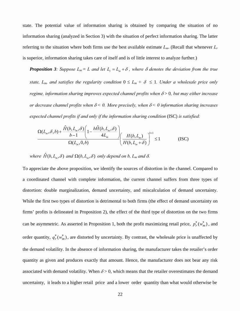
Proposition 3: Suppose Lm = L and let r mL L δ= + , where δ denotes the deviation from the true

state, Lm, and satisfies the regularity condition 0 ≤ Lm + δ ≤ 1. Under a wholesale price only

regime, information sharing improves expected channel profits when δ > 0, but may either increase

or decrease channel profits when δ < 0. More precisely, when δ < 0 information sharing increases

expected channel profits if and only if the information sharing condition (ISC) is satisfied:

1

ˆ ˆ( , , ) ( , , )( , , ) 11 4 ( , ) 1

( ,0, ) ( , )

m mbm

m m

m m

H b L bH b LL bb L H b L

L b H b L

δ δδ

δ

+

⎛ ⎞Ω + −⎜ ⎟− ⎛ ⎞⎝ ⎠ ≤⎜ ⎟Ω +⎝ ⎠

(ISC)

where ˆ ( , , )mH b L δ and ( , , )mb L δΩ only depend on b, Lm and δ.

To appreciate the above proposition, we identify the sources of distortion in the channel. Compared to

a coordinated channel with complete information, the current channel suffers from three types of

distortion: double marginalization, demand uncertainty, and miscalculation of demand uncertainty.

While the first two types of distortion is detrimental to both firms (the effect of demand uncertainty on

firms’ profits is delineated in Proposition 2), the effect of the third type of distortion on the two firms

can be asymmetric. As asserted in Proposition 1, both the profit maximizing retail price, )( *m

*r wp , and

order quantity, )( *m

*r wq , are distorted by uncertainty. By contrast, the wholesale price is unaffected by

the demand volatility. In the absence of information sharing, the manufacturer takes the retailer’s order

quantity as given and produces exactly that amount. Hence, the manufacturer does not bear any risk

associated with demand volatility. When δ > 0, which means that the retailer overestimates the demand

uncertainty, it leads to a higher retail price and a lower order quantity than what would otherwise be

23

πΔ

δ0 1−1

rπΔ

mπΔ

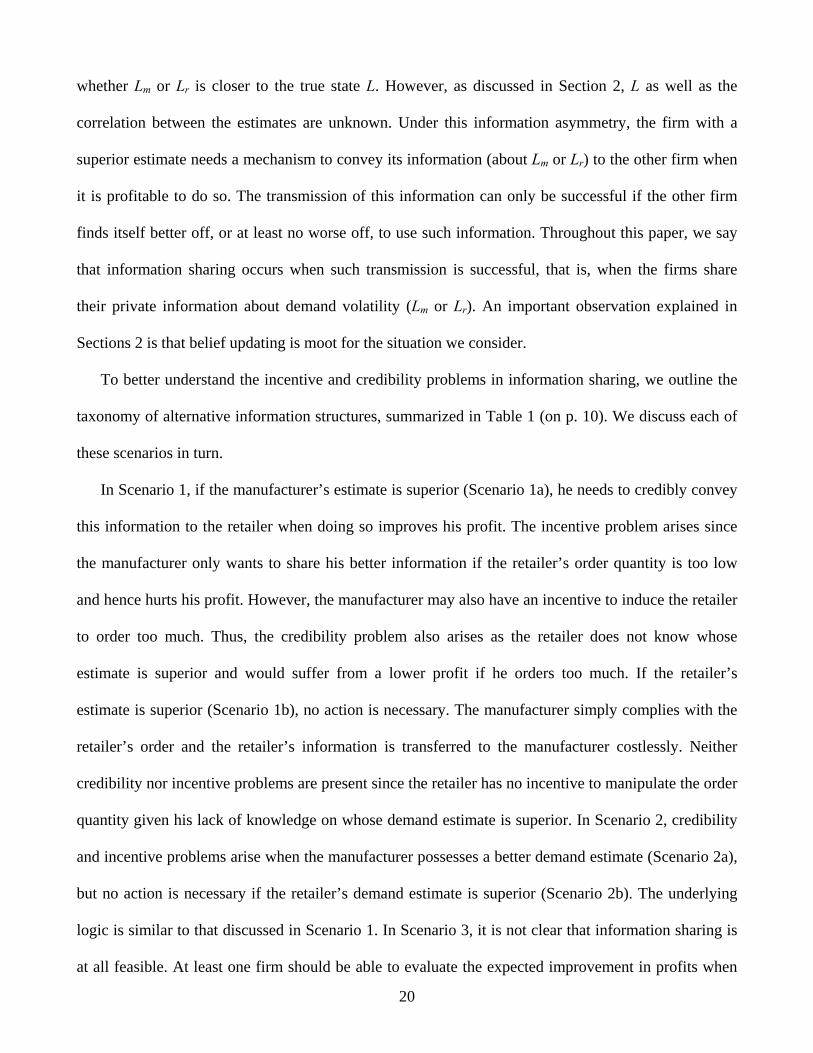
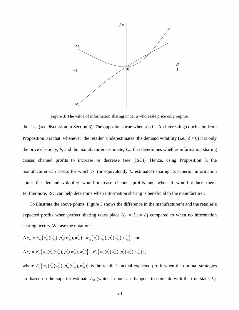
Figure 3: The value of information sharing under a wholesale price only regime.

the case (see discussion in Section 3). The opposite is true when δ < 0. An interesting conclusion from

Proposition 3 is that whenever the retailer underestimates the demand volatility (i.e., δ < 0) it is only

the price elasticity, b, and the manufacturers estimate, Lm, that determines whether information sharing

causes channel profits to increase or decrease (see (ISC)). Hence, using Proposition 3, the

manufacturer can assess for which δ (or equivalently Lr estimates) sharing its superior information

about the demand volatility would increase channel profits and when it would reduce them.

Furthermore, ISC can help determine when information sharing is beneficial to the manufacturer.

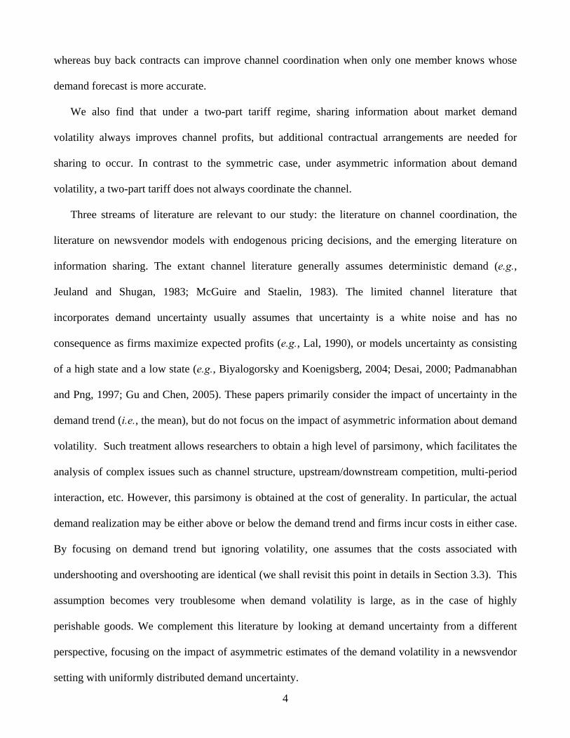
To illustrate the above points, Figure 3 shows the difference in the manufacturer’s and the retailer’s

expected profits when perfect sharing takes place (Lr = Lm = L) compared to when no information

sharing occurs. We use the notation:

( ) ( )* * * * * * * * * *( ), ( ), ( ), ( ),m m m m m m m m r m r m mz w p w w z w p w wπ π πΔ = − , and

{ } { }* * * * * * * * * *( ( ), ( ), ) ( ( ), ( ), )r r m m m m m r r m r m mE z w p w w E z w p w wε επ π πΔ = − ,

where { }* * * * *( ( ), ( ), )r m m m m mE z w p w wε π is the retailer’s actual expected profit when the optimal strategies

are based on the superior estimate Lm (which in our case happens to coincide with the true state, L).

24

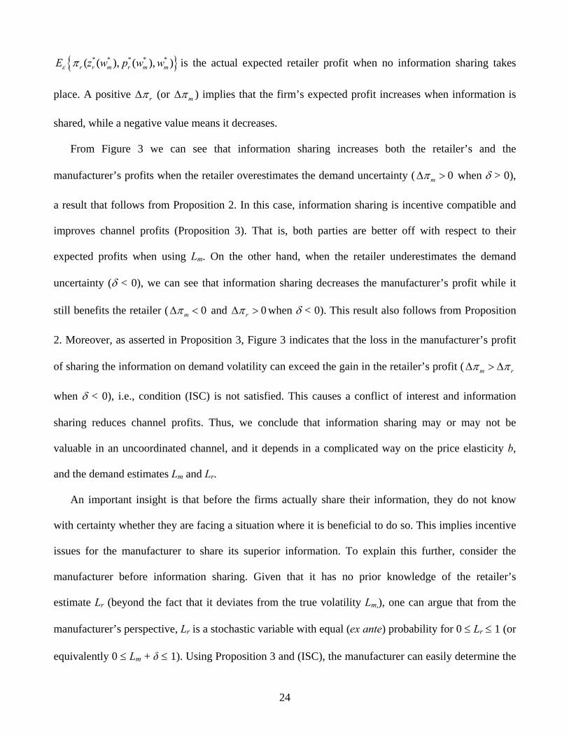
{ }* * * * *( ( ), ( ), )r r m r m mE z w p w wε π is the actual expected retailer profit when no information sharing takes

place. A positive rπΔ (or mπΔ ) implies that the firm’s expected profit increases when information is

shared, while a negative value means it decreases.

From Figure 3 we can see that information sharing increases both the retailer’s and the

manufacturer’s profits when the retailer overestimates the demand uncertainty ( 0mπΔ > when δ > 0),

a result that follows from Proposition 2. In this case, information sharing is incentive compatible and

improves channel profits (Proposition 3). That is, both parties are better off with respect to their

expected profits when using Lm. On the other hand, when the retailer underestimates the demand

uncertainty (δ < 0), we can see that information sharing decreases the manufacturer’s profit while it

still benefits the retailer ( 0mπΔ < and 0rπΔ > when δ < 0). This result also follows from Proposition

2. Moreover, as asserted in Proposition 3, Figure 3 indicates that the loss in the manufacturer’s profit

of sharing the information on demand volatility can exceed the gain in the retailer’s profit ( m rπ πΔ > Δ

when δ < 0), i.e., condition (ISC) is not satisfied. This causes a conflict of interest and information

sharing reduces channel profits. Thus, we conclude that information sharing may or may not be

valuable in an uncoordinated channel, and it depends in a complicated way on the price elasticity b,

and the demand estimates Lm and Lr.

An important insight is that before the firms actually share their information, they do not know

with certainty whether they are facing a situation where it is beneficial to do so. This implies incentive

issues for the manufacturer to share its superior information. To explain this further, consider the

manufacturer before information sharing. Given that it has no prior knowledge of the retailer’s

estimate Lr (beyond the fact that it deviates from the true volatility Lm,), one can argue that from the

manufacturer’s perspective, Lr is a stochastic variable with equal (ex ante) probability for 0 ≤ Lr ≤ 1 (or

equivalently 0 ≤ Lm + δ ≤ 1). Using Proposition 3 and (ISC), the manufacturer can easily determine the

25

range of δ where information sharing increases and decreases expected channel profits, respectively,

and thus the probability for information sharing to be beneficial. For example, if Lm < 0.5 we know

without using condition (ISC) that there is at least a 50% chance information sharing will increase the

expected channel profits (the probability that δ>0 is 1−Lm). One can therefore argue that in this case it

is rational for the manufacturer to share its information. (Note that this argument is not contingent on

Lm = L, since the L is unknown and Lm is the best estimate available when the manufacturer makes its

decision.) However, for certain values of Lm and b sharing is bound to not take place because the

manufacturer concludes that there is a larger chance profits will decrease than increase.

As an alternative, before sharing the manufacturer can also compute the expected gain in channel

profits across the entire range of feasible δ values (for example using the expressions specified in the

proof of Proposition 3 and integrate numerically). If this gain is positive it would be rational for the

manufacturer to share information, otherwise not.

To conclude, it is not obvious that the manufacturer is always willing to share its superior

information since doing so may improve the retailer’s profit at the expense of reducing its own profit.

Although information sharing reduce/eliminate the distortion caused by the miscalculation of demand

uncertainty, its impact on the profits of the manufacturer and the retailer is asymmetric. In particular,

information sharing is not incentive compatible when the retailer underestimates demand volatility. In

sum, information sharing is feasible only when it benefits both firms, i.e., when the information

sharing condition illustrated in Proposition 3 holds.

4.2 Information Sharing Contracts

As discussed earlier, firms need to overcome incentive and credibility problems to achieve

information sharing. In what follows, we investigate two alternative contractual arrangements that help

achieve information sharing. In particular, these contracts are relatively easy to implement. We first

analyze the profit sharing contract when the quality of the demand estimates is common knowledge;

26

we then examine the buy back contract when only one firm knows whose demand estimate is superior.

In addition, we study the effect of information sharing on pricing, firms’ profits, and channel profits.

4.2.1 The profit sharing contract

When both the manufacturer and the retailer know which demand estimate is superior, credibility is

not an issue but the incentive problem remains. A profit sharing contract is a simple mechanism to

facilitate information sharing under such circumstances. Since information sharing takes care of itself

when the retailer’s estimate is superior, we only consider the case when the manufacturer’s estimate is

superior. Our analysis presumes that the manufacturer has an interest in sharing. (As explained in

Section 3.1., this is not always the case since the manufacturer may conclude before the fact that the

risk of reducing the expected channel profit is too high.) The sequence of actions is as follows. First,

the manufacturer and the retailer negotiate for a division of the combined gain in profits when

information sharing occurs. The gain (loss) in profit for each firm is relative to the no information

sharing case, where the firms use their own demand estimates. Although the division can be arbitrary

depending on each firm’s bargaining power, we assume without loss of generality that both firms split

the gain equally. If the negotiation is successful, both firms submit their demand estimates

simultaneously. Otherwise, the firms do not reveal their demand estimates and the game proceeds as in

the no-information-sharing case described in Section 3. The solution concept in the profit sharing

contract is one of Nash bargaining. Without information sharing, the equilibrium strategy

( * * * * *( ), ( ),r m r m mz w p w w ) is based on the retailers demand estimate. With information sharing, both firms

use the superior estimate Lm when determining the optimal strategy ( * * * * *( ), ( ),m m m m mz w p w w ). After the

demand estimates are revealed both parties agree that Lm is the best available estimate of the true

demand volatility. Under this estimate the retailer’s expected profit with and without information

sharing are { }* * * * *( ( ), ( ), )m r m m m m mE z w p w wε π and { }* * * * *( ( ), ( ), )

m r r m r m mE z w p w wε π respectively. Similarly the

manufacturer’s profit with and without information sharing are ( )* * * * *( ), ( ),m m m m m mz w p w wπ and

27

( )* * * * *( ), ( ),m r m r m mz w p w wπ . Hence, after the contract is signed (in our case after the fifty-fifty split is

agreed on), the firms’ perceived change in the expected total channel profits is

{ } { }( )( ) ( )( )

* * * * * * * * * *

* * * * * * * * * *

( ( ), ( ), ) ( ( ), ( ), )

( ), ( ), ( ), ( ),

m mr m m m m m r r m r m m

m m m m m m m r m r m m

E z w p w w E z w p w w

z w p w w z w p w w

ε επ π

π π

ΔΠ = −

+ − (15)

and the profit sharing contract dictates that the manufacturer and the retailer each receives 12ΔΠ in

equilibrium.

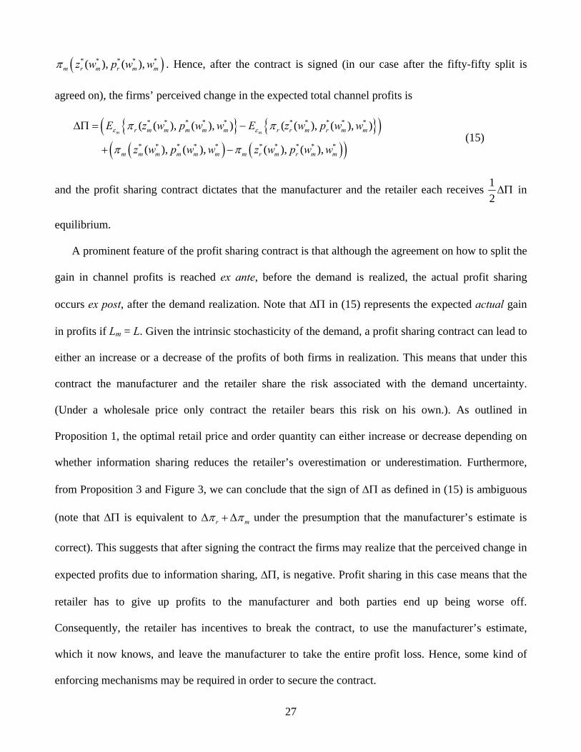
A prominent feature of the profit sharing contract is that although the agreement on how to split the

gain in channel profits is reached ex ante, before the demand is realized, the actual profit sharing

occurs ex post, after the demand realization. Note that ΔΠ in (15) represents the expected actual gain

in profits if Lm = L. Given the intrinsic stochasticity of the demand, a profit sharing contract can lead to

either an increase or a decrease of the profits of both firms in realization. This means that under this

contract the manufacturer and the retailer share the risk associated with the demand uncertainty.

(Under a wholesale price only contract the retailer bears this risk on his own.). As outlined in

Proposition 1, the optimal retail price and order quantity can either increase or decrease depending on

whether information sharing reduces the retailer’s overestimation or underestimation. Furthermore,

from Proposition 3 and Figure 3, we can conclude that the sign of ΔΠ as defined in (15) is ambiguous

(note that ΔΠ is equivalent to r mπ πΔ + Δ under the presumption that the manufacturer’s estimate is

correct). This suggests that after signing the contract the firms may realize that the perceived change in

expected profits due to information sharing, ΔΠ, is negative. Profit sharing in this case means that the

retailer has to give up profits to the manufacturer and both parties end up being worse off.

Consequently, the retailer has incentives to break the contract, to use the manufacturer’s estimate,

which it now knows, and leave the manufacturer to take the entire profit loss. Hence, some kind of

enforcing mechanisms may be required in order to secure the contract.

28

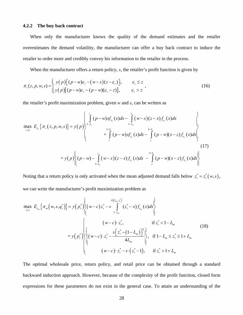
4.2.2 The buy back contract

When only the manufacturer knows the quality of the demand estimates and the retailer

overestimates the demand volatility, the manufacturer can offer a buy back contract to induce the

retailer to order more and credibly convey his information to the retailer in the process.

When the manufacturer offers a return policy, s, the retailer’s profit function is given by

( ) ( )( )[ ]

( ) ( ) , ( , , , )

( ) ( )( ) , r r r

rr r r

y p p w w s z zz p w s

y p p w p w z z

ε ε επ

ε ε ε

⎧ − − − − ≤⎡ ⎤⎪ ⎣ ⎦= ⎨− − − − >⎪⎩

, (16)

the retailer’s profit maximization problem, given w and s, can be written as

( ){ } ( )( )

1 1

1 1,

( ) ( ) ( ) ( )

max , , ,

+ ( ) ( ) ( )( ) ( )

r r

r r

r r r

r r

z z

L Lr L Lz p

z z

p w xf x dx w s z x f x dx

E z p w s y p

p w xf x dx p w x z f x dx

ε ε

ε

ε ε

π − −

+ +

⎧ ⎫− − − −⎪ ⎪

⎪ ⎪= ⎨ ⎬⎪ ⎪− − − −⎪ ⎪⎩ ⎭

∫ ∫

∫ ∫

( ) ( )1

1

= ( ) ( ) ( ) ( )( ) ( )r

r r

r

Lz

L z

y p p w w s z x f x dx p w x z f x dxε ε

+

−

⎧ ⎫⎪ ⎪− − − − − − −⎨ ⎬⎪ ⎪⎩ ⎭

∫ ∫

(17)

Noting that a return policy is only activated when the mean adjusted demand falls below ( )* * ,r rz z w s= ,

we can write the manufacturer’s profit maximization problem as

( ){ } ( ) ( )( )

( )

( )

( )( )

*,

* * * *

,1

* *

2** *

max , , ( ) ( )

, if 1

1 = , if 1

4

m r

m m

m

G L z

m r r r rw sL

r r m

r mr r m

m

E w s q y p w c z s z x f x dx

w c z z L

s z Ly p w c z L

L

ε επ−

⎧ ⎫⎪ ⎪= − − −⎨ ⎬⎪ ⎪⎩ ⎭

− ⋅ < −

⎧ ⎫⎡ ⎤− −⎪ ⎪⎣ ⎦− ⋅ − −⎨ ⎬⎪ ⎪⎩ ⎭

∫

( ) ( )

*

* * *

1

1 , if 1

r m

r r r m

z L

w c z s z z L

⎧⎪⎪⎪ ≤ ≤ +⎨⎪⎪⎪ − ⋅ − ⋅ − > +⎩

(18)

The optimal wholesale price, return policy, and retail price can be obtained through a standard

backward induction approach. However, because of the complexity of the profit function, closed form

expressions for these parameters do not exist in the general case. To attain an understanding of the

29

behavior of )s,w(p*r and )s,w(q*

r we therefore focus on the special case where Lr=1 and we can

derive analytical results.

Proposition 4: Given w, and Lr=1, the optimal retail price )s,w(p*r is decreasing in the return

policy s and the optimal order quantity )s,w(q*r is increasing in the return policy s.

Proposition 4 asserts that for any given wholesale price, the manufacturer can offer a return policy

to induce the retailer to charge a lower retail price and order more. Hence, when pricing is endogenous

a return policy will stimulate larger retailer orders. The manufacturer will only offer a return policy

that improves its expected profit (18). Similarly, the retailer will only accept a policy that improves its

expected profit (17). This implies that by offering a return policy, the retailer’s overestimation of

demand volatility is reduced, and the expected profits for both firms are improved. Although we are

able to demonstrate these relationships analytically only for Lr = 1, our numerical studies suggest that

Proposition 3 holds for any Lr > Lm. Padmanabhan and Png (1997) and Emmons and Gilbert (1998)

show similar relationships under symmetric demand information. Consequently, our results

demonstrate that a return policy helps to achieve information sharing under asymmetric information,

and continues to be an effective tool for channel coordination. We note, however, that a return policy is

generally not as efficient as other types of contracts such as the profit sharing contract and the two-part

tariff (discussed in Section 5). The intuition is as follows. A return policy impacts the optimal

wholesale price and retail price, thereby inducing the retailer to place a larger order. The distortion of

the pricing decisions results in deadweight loss. By contrast, a profit sharing contract achieves

information sharing through a fixed fee, which is free from distortion and deadweight loss. However,

the key advantage of the return policy is the ease of implementation, which probably explains the

popularity of this type of policy in real world practice.

30

5. A Two-part Tariff Regime

In Section 4, we examine the value of information sharing, and some contracts to facilitate sharing

in an uncoordinated channel operating under a wholesale price only regime. We now turn to an

alternative two-part tariff regime. Under a bilateral monopoly and symmetric information, it is well

known (e.g., Locay and Rodriguez (1992), Raju and Zhang (2005)) that the optimal two-part tariff is in

the form of the manufacturer charging the retailer a fixed fee and a wholesale price at the marginal cost.

A wholesale price at the marginal cost eliminates double marginalization and ensures maximum

channel profits. The fixed fee serves to split the channel profits between the manufacturer and the

retailer. It is worth noting that under asymmetric information about the demand volatility the firms

have different perceptions of the expected channel profits. From the manufacturer’s perspective the

expected channel profit before information sharing is { }* *( ( ), ( ), )m r m mE z c p c cε π , and the fixed fee can be

expressed as { }* *( ( ), ( ), )mm r m mE z c p c cεθ π , where ( )0,1mθ ∈ . Because the wholesale price is c, without

the fixed fee the manufacturer’s profit is zero. From the retailers perspective the expected channel

profit is { }* *( ( ), ( ), )r r r rE z c p c cε π and the fixed fee is { }* *( ( ), ( ), )

rr r r rE z c p c cεθ π , with ( )0,1rθ ∈ . The

actual expected channel profit, unknown to the firms, is { }* *( ( ), ( ), )r r rE z c p c cε π . In order to do business,

the firms must agree on the fixed fee, i.e., { }* *( ( ), ( ), )mm r m mE z c p c cεθ π = { }* *( ( ), ( ), )

rr r r rE z c p c cεθ π . Note

that unless Lr = Lm, the negotiated fee constitutes different portions of the firms’ perceived channel

profits, i.e., mθ ≠ rθ . The size of the fee clearly depends on the firms’ bargaining power, which may be

influenced by the quality of the demand information and knowledge thereof, i.e., which firm has the

superior demand estimate and which knows about this. However, as we asserted in Section 4, a

detailed treatment of bargaining is beyond the scope of this paper.

31

πΔ

δ0 1-1

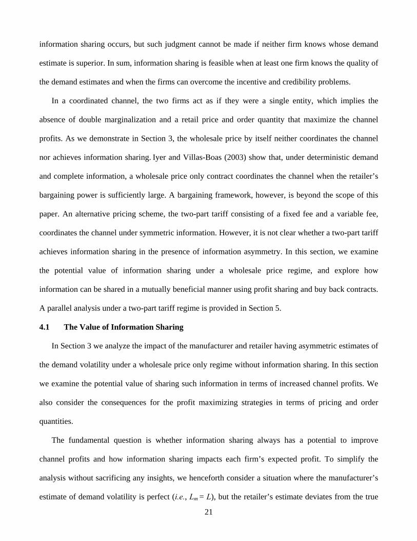
Figure 4: The value of information sharing under a two-part tariff regime.

Clearly, a two-part tariff coordinates the channel when the manufacturer and the retailer have

symmetric information (i.e., Lr = Lm and mθ = rθ ). This is because the wholesale price is set to the

marginal cost and the manufacturer derives his profit solely from the fixed fee, which is a portion of

the retailer’s expected profit. As a result, maximizing the retailer’s expected profit amounts to

maximizing the expected channel profits. In the absence of information asymmetry, the manufacturer

concurs with the retailer’s perceived expected profit. Thus, there is no disagreement regarding the

portion of the channel profits that constitute the fixed fee.

As under the wholesale price regime in Section 4, a fundamental question under a two-part tariff

regime is the potential for information sharing to improve expected channel profits, and how that

impacts the firms’ individual profits. Noting that the expected channel profit equals the retailer’s

expected profit, it follows that information sharing as defined in this paper only affects the channel

profit when the manufacturer’s estimate Lm is superior. To assess the value of information sharing we

therefore follow the approach in Section 4 and compare the situation of no information sharing with

that of perfect information sharing where both firms use the superior estimate Lm=L.

32

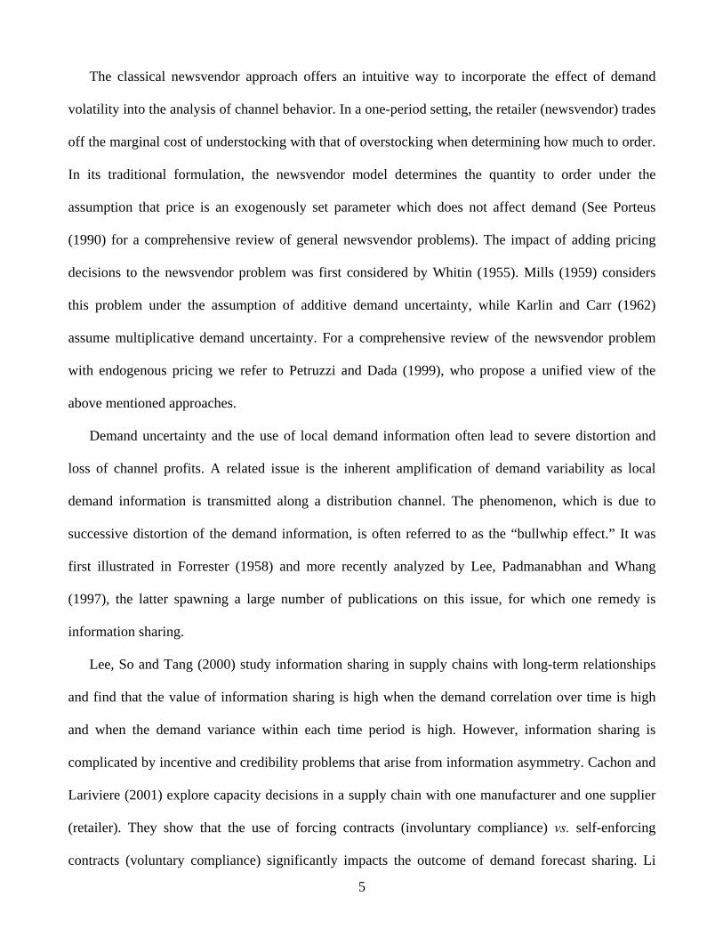
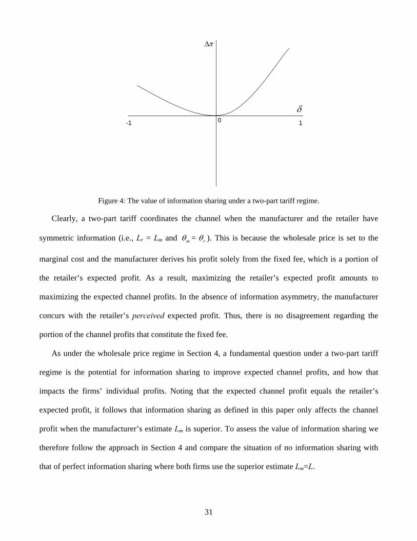
Lemma 4: Under a two-part tariff, perfect information sharing always improves the expected

channel profits.

Without information sharing, the expected channel profit is equivalent to the retailer’s actual

expected profit { }* *( ( ), ( ), )r r rE z c p c cε π where the pricing and order decisions are based on the retailer’s

demand estimate, Lr. Consistent with Proposition 2, both overestimation and underestimation of the

demand volatility are detrimental to the retailer’s actual expected profit and therefore also to the

channel (Figure 4). When the manufacturer shares its superior demand information Lm with the retailer

the expected channel profit increases and creates an opportunity for both firms to be better off than

before. It is not clear, however, whether a two-part tariff suffices to achieve information sharing when

the manufacturer and the retailer have different demand estimates, which is the case in our model. We

therefore, need to further examine when (if ever) a two-part tariff coordinates the channel under

asymmetric demand information. We address these issues next, for each option in our information

sharing taxonomy outlined in Table 1.

Proposition 5:

(i) If the quality of the demand volatility estimates is private information, a two-part tariff

achieves information sharing and coordinates the channel in Scenario 1b and Scenario 2a; in

Scenario 1a, Scenario 2b, and Scenario 3, it does not achieve information sharing but it may

coordinate the channel if there is no dispute about the fixed fee.

(ii) If the quality of the estimates of demand volatility is common knowledge, a two-part tariff

achieves information sharing and coordinates the channel through a profit sharing contract.

When firms have asymmetric demand estimates, a two-part tariff does not always achieve

information sharing and fails to coordinate the channel under certain conditions. This is in contrast to

the situation under symmetric information, where a two-part tariff always coordinates the channel. The

intuitions are as follows. When each firm has its own demand forecast, it also has an asymmetric

33

forecast of the total channel profits, and this in turn may lead to disagreement on the amount of fixed

fee. When the quality of the demand estimates is private information, a two-part tariff by itself cannot

resolve such dispute.

Under a two-part tariff, the incentive problem in a profit sharing contract is relatively simple. Since

information sharing always improves the expected channel profits (Figure 4), the firms only need to

negotiate an agreement on how to split the benefits from information sharing. However, a profit

sharing contract is feasible only when the quality of demand estimates is common knowledge. It is

interesting to compare the properties of a two-part tariff with those of a profit sharing contract. A two-

part tariff is strictly an ex ante contract, both the wholesale price and the fixed fee are set before the

demand realization. By contrast, a profit sharing contract has both ex ante and ex post components.

While the terms of the contracts are determined before the demand realization, the execution of the

contract occurs after the demand realization. Therefore, a two-part tariff is risk free to the manufacturer,

whereas a profit sharing contract leads to risk sharing between the manufacturer and the retailer.

6. Conclusion

As Padmanabhan and Png (1997) eloquently put it, “one of the few certainties about the demand

for products such as new books, CDs, software, fashion wear, and winter clothing is that it is

uncertain.” Fortunately, many of the results from the extant channel literature remain robust with or

without demand uncertainty. However, important questions arise when firms in a distribution channel

face asymmetric demand uncertainty: should this information be shared, what is the value of sharing,

and how can sharing be accomplished? In this paper, we provide insights into these issues. Rather than

looking at uncertainty about demand trend, we focus on firms’ asymmetric information on demand

volatility. Specifically, we consider a situation with price dependent multiplicative demand uncertainty

where firms are correct in estimating the average demand trend, but they may miscalculate the extent

of demand volatility. The value of information sharing stems from the fact that one member of the

34

distribution channel may possess a superior estimate of the demand volatility compared to the other

member. However, the firms may not possess the same information on whose demand estimate is

superior. This asymmetric information on the quality of the demand estimates further complicates

information sharing. In the context of bilateral monopoly and short-term relationships, we demonstrate

through our model that demand volatility can have substantial impact on retail price, order quantity,

and the firms’ profits. Although information sharing always improves channel profits in a coordinated

channel, it is not necessarily so if the channel is uncoordinated because of asymmetric demand

information. Depending on the specific information structure, there are different strategies and

contracts that firms can use to facilitate information sharing. Two prominent examples that we

consider in this work are profit sharing contracts and return policies.

There are several directions to extend our model. In this paper, we consider a channel of bilateral

monopoly in a single period setting, it is interesting to investigate how upstream and downstream

competition moderate information sharing; it is also interesting to use a signaling framework to

examine information sharing in a multi-period setting. Although pricing is a decision variable in our

model, we do not consider retail promotion. An important form of uncertainty not covered in the paper

is the uncertainty stemming from lead-time and capacity constraint. It would also be interesting to

investigate the impact of using other types of demand models, additive demand uncertainty, alternative

distributions etc. Finally, many alternative contracts, such as quantity discount contracts, are good

candidates for achieving information sharing. We leave these issues to future research.

35

Appendix: Proofs

Proof of Claim 1:

Suppose a firm’s estimate of L follows a distribution g(L) with positive support over the interval

,L L⎡ ⎤⎣ ⎦ , with 0L ≥ and L L< . Since demand is uniformly distributed over the interval

[ ]( )(1 ), ( )(1 )y p L y p L− + , it follows that the firm’s estimated distribution of ε equals

( ) ( | ) ( )L

L

f x f x L g L dL= ∫ , where

1 if 1 1( | ) 2

0 otherwise

L x Lf x L L

⎧ − ≤ ≤ +⎪= ⎨⎪⎩

represents the pdf given a bound L on the uniform distribution.

As a result, for any g(L) the implied distribution from the above expression is not uniform, since

( ) ( )f L f L≠ + for any such that 0 L L< ≤ − . Given that we assume that it is common knowledge

that ε is uniformly distributed, any estimate that follows some distribution with positive support over

some interval will therefore yield a contradiction. Q.E.D.

Proof of Claim 2:

Refer to Section 3.2.

Proof of Claim 3:

Without information sharing, the retailer cannot extract any additional information from the

manufacturer since the wholesale price w is uninformative. Because iL can be either greater than or

less than the true state L, the retailer has no way of knowing which way she should adjust rL even

when rσ dictates that the manufacturer is of type h. In a long-term relationship, an update is possible

by using the correlation between mε and rε based on historical data. However, such correlation is

unknown in the one-shot setting we consider. Therefore, it is rational for the retailer to base her

decisions on her own estimate rL .

36

By the same token, the decision rule for the retailer as to whether to base her decisions on mL or

rL when information sharing occurs is as follows. She would use mL if

( ){ } ( ){ }, ,r m r r r r r rE L L E L Lπ σ π σ≥ . Otherwise she would continue to base her decisions on rL .

Q.E.D.

Proof of Lemma 1:

After substituting *( , )rz p w into expression (4), we take the first derivative of the retailer’s expected

profit function with respect to p, yielding

{ }*

2

2

( ) ( )( ( , ), )

( )( ) ( ) ( )

( ) ( ) ( ) 1

1 ( )

r r r

p wy p p w LwE z p w p p

p p

p wp w Lwpy p p wp w Lw y p

p p p

b p w Lwy p p w Lw y pp p p

y p

π⎡ ⎤⎛ ⎞−

∂ − −⎢ ⎥⎜ ⎟∂ ⎝ ⎠⎣ ⎦=∂ ∂

⎛ ⎞−∂ − −⎜ ⎟⎛ ⎞∂ − ⎝ ⎠= − − +⎜ ⎟∂ ∂⎝ ⎠⎛ ⎞⎛ ⎞− −

= − − + −⎜ ⎟⎜ ⎟⎝ ⎠ ⎝ ⎠

= ( )2 22 (1 ) ( 1) ( 1) ,

b p bw L p b w Lp

⎛ ⎞− + + + +⎜ ⎟

⎝ ⎠

and use the first-order optimality conditions to obtain

{ }*2 2

( ( , ), )0 1 1 1 0 r r rE z p w p

( b)p bw(L )p (b )w Lp

π∂= ⇒ − + + + + =

∂.

Solving for the resulting equality for p yields

2 2* *

2 2

1 1 1 1( ) or ( )1 2 2 1 2 2r r

b L L L b L L Lp w w p w wb b b b

⎛ ⎞ ⎛ ⎞+ − + −⎛ ⎞ ⎛ ⎞⎜ ⎟ ⎜ ⎟= + + = − +⎜ ⎟ ⎜ ⎟⎜ ⎟ ⎜ ⎟− −⎝ ⎠ ⎝ ⎠⎝ ⎠ ⎝ ⎠The

additional constraint *( )rp w w≥ , however, ensures that only the first of these expressions is valid. To

show this, we first note that wp ≥* holds for the first solution, since

37

2 2

2 2

1 1 1 1 1 1 and therefore 12 2 2 2 2 2

L L L L L L L Lb b

− − + − + −⎛ ⎞ ⎛ ⎞+ > + + > + =⎜ ⎟ ⎜ ⎟⎝ ⎠ ⎝ ⎠

On the other hand, using the same logic for the second expression yields

2

2

1 1 1 1 ,2 2 2 2

L L L L L Lb

+ − + −⎛ ⎞− + < − =⎜ ⎟⎝ ⎠

and therefore this solution is invalid if 1bLb−

≤ . Suppose therefore that 1bLb−

> . Then,

2

2

1 1 1 2 2

L L L bb b

+ − −⎛ ⎞− + ≥⎜ ⎟⎝ ⎠

implies

2

2

1 1 1 2 (1 ) ,2 2 2

L L L b L bb b b

− + − − −⎛ ⎞ + ≤ − =⎜ ⎟⎝ ⎠

and therefore (since 1bLb−

> implies 2 (1 ) 0L b− − > ),

2 2 2 2

2 2

(1 ) 4 4 4(1 ) (1 ) ,4 4

rb L L L b L bb b

− + − − + −≤

or

4 1 4 1( - L)b ( L),≤ −

which contradicts our assumption that b > 1. Thus, the second expression for the optimal price is never

valid. Q.E.D.

Proof of Lemma 2:

*

*

*

( ( ), ) 1

21 0( )

( ) 21( , ) 2

r

r

r

z p w w

wLp w

p w wbH b L

b

>⇔

⎛ ⎞− >⎜ ⎟

⎝ ⎠⇔

>⇔

−>

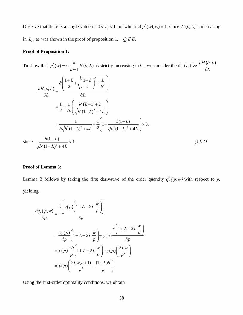
38

Observe that there is a single value of 0 1rL< < for which *( ( ), ) 1rz p w w = , since ( , )H b L is increasing

in rL , as was shown in the proof of proposition 1. Q.E.D.

Proof of Proposition 1:

To show that *( ) ( , )1r

bp w w H b Lb

=−

is strictly increasing in rL , we consider the derivative ( , )H b LL

∂∂

2

2

2

2 2

2 2 2 2

1 12 2( , )

1 1 ( 1) 22 2 (1 ) 4

1 1 (1 )1 0,2(1 ) 4 (1 ) 4

r

L L LbH b L

L L

b Lb b L L

b Lb b L L b L L

⎛ ⎞+ −⎛ ⎞⎜ ⎟∂ + +⎜ ⎟⎜ ⎟⎝ ⎠∂ ⎝ ⎠=∂ ∂

⎛ ⎞− +⎜ ⎟= +⎜ ⎟− +⎝ ⎠

⎛ ⎞−⎜ ⎟= + − >⎜ ⎟− + − +⎝ ⎠

since 2 2

(1 ) 1.(1 ) 4b L

b L L−

<− +

Q.E.D.

Proof of Lemma 3:

Lemma 3 follows by taking the first derivative of the order quantity )w,p(q*r with respect to p,

yielding

*

2

2

( ) 1 2( , )

1 2( ) 1 2 ( )

2 ( ) 1 2 ( )

2 ( 1) (1 ) ( ) .

r

wy p L Lpq p w

p p

wL Lpy p wL L y p

p p p

b w Lwy p L L y pp p p

Lw b L by pp p

⎡ ⎤⎛ ⎞∂ + −⎢ ⎥⎜ ⎟

∂ ⎝ ⎠⎣ ⎦=∂ ∂

⎛ ⎞∂ + −⎜ ⎟⎛ ⎞∂ ⎝ ⎠= + − +⎜ ⎟∂ ∂⎝ ⎠

⎛ ⎞ ⎛ ⎞−= + − +⎜ ⎟ ⎜ ⎟

⎝ ⎠ ⎝ ⎠⎛ ⎞+ +

= −⎜ ⎟⎝ ⎠

Using the first-order optimality conditions, we obtain

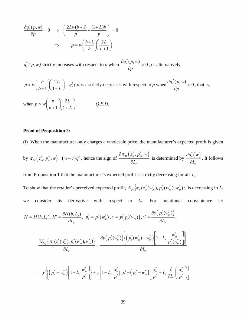
39

*

2

( , ) 2 ( 1) (1 )0 0

1 21

rq p w Lw b L bp p p

b Lp wb L

⎛ ⎞∂ + += ⇒ − =⎜ ⎟∂ ⎝ ⎠

+⎛ ⎞⎛ ⎞⇒ = ⎜ ⎟⎜ ⎟+⎝ ⎠⎝ ⎠

)w,p(q*r strictly increases with respect to p when 0

),(*

>∂

∂p

wpqr , or alternatively

21 1

b Lp wb L

⎛ ⎞⎛ ⎞< ⎜ ⎟⎜ ⎟+ +⎝ ⎠⎝ ⎠ . )w,p(q*

r strictly decreases with respect to p when 0),(*

<∂

∂p

wpqr , that is,

when 21 1

b Lp wb L

⎛ ⎞⎛ ⎞> ⎜ ⎟⎜ ⎟+ +⎝ ⎠⎝ ⎠. Q.E.D.

Proof of Proposition 2:

(i) When the manufacturer only charges a wholesale price, the manufacturer’s expected profit is given

by ( ) ( )* * *, ,M m m rz p w w c qπ = − , hence the sign of ( )* *, ,M m m

r

z p wL

π∂

∂ is determined by ( )*

r

r

q wL

∂∂

. It follows

from Proposition 1 that the manufacturer’s expected profit is strictly decreasing for all rL .

To show that the retailer’s perceived expected profit, { }),)(,)(( *****mmrmrr wwpwzE

rπε , is decreasing in Lr.

we consider its derivative with respect to Lr. For notational convenience let

),( rLbHH = , ( , )r

r

H b LHL

∂′ =∂

, * * *( )r r mp p w= , ( )* *( )r my y p w= ,( )* *( )r m

r

y p wy

L∂

′ =∂

.

{ } ( ) ( )*

* * * * ** * * * * * *( ) ( ) 1

( ( ), ( ), ) ( )

r

mr m r m m r

r r m r m m r m

r r

wy p w p w w LE z w p w w p w

L Lε π

⎧ ⎫⎡ ⎤⎪ ⎪∂ − −⎨ ⎬⎢ ⎥∂ ⎪ ⎪⎣ ⎦⎩ ⎭=∂ ∂

( ) ( )* * * *

* * * ** * * *1 1m m m m

r m r r r m rr r r r r

w w w wy p w L y L p p w Lp p p L p

⎧ ⎫ ⎡ ⎤⎡ ⎤ ⎡ ⎤ ⎛ ⎞∂⎪ ⎪′ ′= − − + − − − +⎨ ⎬ ⎢ ⎥⎜ ⎟⎢ ⎥ ⎢ ⎥ ∂⎪ ⎪⎣ ⎦ ⎣ ⎦ ⎝ ⎠⎩ ⎭ ⎣ ⎦

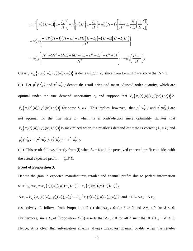
40

( ) ( )* * * 1 11 1 1 1r rm m m r

r

L Ly w H y w H w H LH H H L H

⎧ ⎫⎡ ⎤⎡ ⎤ ∂⎪ ⎪⎛ ⎞ ⎛ ⎞ ⎛ ⎞′ ′= − − + − − − +⎨ ⎬⎢ ⎥⎜ ⎟⎜ ⎟ ⎜ ⎟⎢ ⎥ ∂ ⎝ ⎠⎝ ⎠ ⎝ ⎠⎪ ⎪⎣ ⎦ ⎣ ⎦⎩ ⎭

( )[ ] [ ] ( )[ ]*2

1 1r r rm

bH H H L H H H L H H L Hw y

H′ ′ ′⎧ ⎫− − − + − − − −

= ⎨ ⎬⎩ ⎭

2 2 2* *

2

1r r rm m

H bH bHL bH bL H L H H Hw y w yH H

⎧ ⎫′ ⎡ ⎤− + + − + − − + −⎪ ⎪ ⎛ ⎞⎣ ⎦= = −⎨ ⎬ ⎜ ⎟⎝ ⎠⎪ ⎪⎩ ⎭

Clearly, { }* * * * *( ( ), ( ), )r r r m r m mE z w p w wε π is decreasing in rL since from Lemma 2 we know that H > 1.

(ii) Let )(wp *m

* and )(wz *m

* denote the retail price and mean adjusted order quantity, which are

optimal under the true demand uncertainty ε, and suppose that { }* * * * *( ( ), ( ), )r r m r m mE z w p w wε π ≥

{ }* * * * *( ( ), ( ), )r m m mE z w p w wε π for some rL L≠ . This implies, however, that )(wp *m

* and )(wz *m

* are

not optimal for the true state L, which is a contradiction since optimality dictates that

{ }* * * * *( ( ), ( ), )r r m r m mE z w p w wε π is maximized when the retailer’s demand estimate is correct ( rL = L) and

)(wp *m

*r = )(wp *

m* , )(wz *

m*r = )(wz *

m* .

(iii) This result follows directly from (i) when Lr = L and the perceived expected profit coincides with

the actual expected profit. Q.E.D.

Proof of Proposition 3:

Denote the gain in expected manufacturer, retailer and channel profits due to perfect information

sharing ( ) ( )* * * * * * * * * *( ), ( ), ( ), ( ),m m m m m m m m r m r m mz w p w w z w p w wπ π πΔ = − ,

{ } { }* * * * * * * * * *( ( ), ( ), ) ( ( ), ( ), )m mr r m m m m m r r m r m mE z w p w w E z w p w wε επ π πΔ = − , and m rπ πΔΠ = Δ + Δ ,

respectively. It follows from Proposition 2 (i) that 0mπΔ ≥ for δ ≥ 0 and 0mπΔ < for δ < 0.

Furthermore, since Lm=L Proposition 2 (ii) asserts that 0rπΔ ≥ for all δ such that 0 ≤ Lm + δ ≤ 1.

Hence, it is clear that information sharing always improves channel profits when the retailer

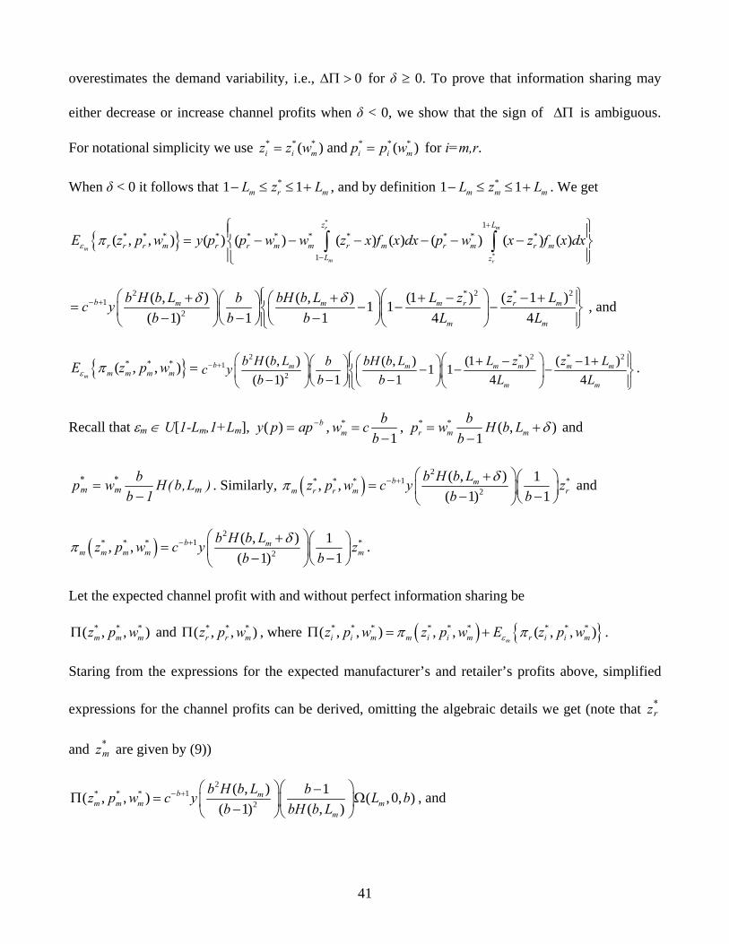
41

overestimates the demand variability, i.e., 0ΔΠ > for δ ≥ 0. To prove that information sharing may

either decrease or increase channel profits when δ < 0, we show that the sign of ΔΠ is ambiguous.

For notational simplicity we use * * * * * *( ) and ( )i i m i i mz z w p p w= = for i=m,r.

When δ < 0 it follows that *1 1m r mL z L− ≤ ≤ + , and by definition *1 1m m mL z L− ≤ ≤ + . We get

{ }*

*

1* * * * * * * * * * *

1

( , , ) ( ) ( ) ( ) ( ) ( ) ( ) ( )mr

m

m r

Lz

r r r m r r m m r m r m r mL z

E z p w y p p w w z x f x dx p w x z f x dxε π+

−

⎧ ⎫⎪ ⎪= − − − − − −⎨ ⎬⎪ ⎪⎩ ⎭

∫ ∫

2 * 2 * 21

2

( , ) ( , ) (1 ) ( 1 )1 1( 1) 1 1 4 4

b m m m r r m

m m

b H b L bH b L L z z Lbc yb b b L L

δ δ− + ⎧ ⎫⎛ ⎞⎛ ⎞+ + + − − +⎪ ⎪⎛ ⎞⎛ ⎞= − − −⎨ ⎬⎜ ⎟⎜ ⎟⎜ ⎟ ⎜ ⎟− − −⎝ ⎠ ⎝ ⎠⎪ ⎪⎝ ⎠ ⎝ ⎠⎩ ⎭ , and

{ }* * *( , , )m m m m mE z p wε π =

2 * 2 * 21

2

( , ) ( , ) (1 ) ( 1 )1 1( 1) 1 1 4 4

b m m m m m m

m m

b H b L bH b L L z z Lbc yb b b L L

− + ⎧ ⎫⎛ ⎞⎛ ⎞ + − − +⎪ ⎪⎛ ⎞⎛ ⎞ − − −⎨ ⎬⎜ ⎟⎜ ⎟⎜ ⎟ ⎜ ⎟− − −⎝ ⎠ ⎝ ⎠⎪ ⎪⎝ ⎠ ⎝ ⎠⎩ ⎭.

Recall that εm ∈ U[1-Lm,1+Lm], bappy −=)( , *

1mbw c

b=

−, ),(

1** δ+

−= mmr LbH

bbwp and

)L,b(H1b

bwp m*m

*m −= . Similarly, ( )

2* * * 1 *

2

( , ) 1, ,( 1) 1

b mm r r m r

b H b Lz p w c y zb b

δπ − + ⎛ ⎞+ ⎛ ⎞= ⎜ ⎟⎜ ⎟− −⎝ ⎠⎝ ⎠ and

( )2

* * * 1 *2

( , ) 1, ,( 1) 1

b mm m m m m

b H b Lz p w c y zb b

δπ − + ⎛ ⎞+ ⎛ ⎞= ⎜ ⎟⎜ ⎟− −⎝ ⎠⎝ ⎠.

Let the expected channel profit with and without perfect information sharing be

* * *( , , )m m mz p wΠ and * * *( , , )r r mz p wΠ , where ( ) { }* * * * * * * * *( , , ) , , ( , , )mi i m m i i m r i i mz p w z p w E z p wεπ πΠ = + .

Staring from the expressions for the expected manufacturer’s and retailer’s profits above, simplified

expressions for the channel profits can be derived, omitting the algebraic details we get (note that *rz

and *mz are given by (9))

2* * * 1

2

( , ) 1( , , ) ( ,0, )( 1) ( , )

b mm m m m

m

b H b L bz p w c y L bb bH b L

− + ⎛ ⎞⎛ ⎞ −Π = Ω⎜ ⎟⎜ ⎟−⎝ ⎠⎝ ⎠

, and

42

2* * * 1

2

ˆ ˆ( , ) ( , , ) ( , , )1( , , ) ( , , ) 1( 1) ( , ) 1 4

b m m mr r m m

m m

b H b L H L b bH L bbz p w c y L bb bH b L b L

δ δ δδδ

− +⎛ ⎞⎛ ⎞⎛ ⎞⎛ ⎞+ −

Π = Ω + −⎜ ⎟⎜ ⎟⎜ ⎟⎜ ⎟ ⎜ ⎟− + −⎝ ⎠⎝ ⎠ ⎝ ⎠⎝ ⎠

where

( , )ˆ ( , , ) 21m

mbH b LH b L

bδδ δ +⎛ ⎞= −⎜ ⎟−⎝ ⎠

, and

2 2

2

( , ) (1 ) ( , )( , , ) 21 ( 1) ( 1)

m m mm m m

b H b L b L H b Lbb L L Lb b b

δ δδ⎛ ⎞ ⎛ ⎞+ + +

Ω = − − −⎜ ⎟ ⎜ ⎟− − −⎝ ⎠⎝ ⎠.

The condition * * * * * *( , , ) ( , , ) 0m m m r r rz p w z p wΔΠ = Π −Π ≥ can now be simplified into (ISC) which holds if

and only if 0ΔΠ ≥ . (Note that by definition * * *( , , ) 0m m mz p wΠ ≥ )

1

ˆ ˆ( , , ) ( , , )( , , ) 11 4 ( , ) 1

( ,0, ) ( , )

m mbm

m m

m m

H b L bH b LL bb L H b L

L b H b L

δ δδ

δ

+

⎛ ⎞Ω + −⎜ ⎟− ⎛ ⎞⎝ ⎠ ≤⎜ ⎟Ω +⎝ ⎠

(ISC)

It follows that the sign of the expected gain in channel profits ΔΠ is a function of b, Lm and δ, but

independent of c and a. By example, it is easy to show that condition (ISC) may or may not be satisfied

for δ < 0. For example if b = 2 and Lm = 1, (ISC) is satisfied (i.e., 0ΔΠ ≥ ) for all possible δ (−1 < δ <

0). On the other hand for b=1.05, Lm=1, (ISC) is not satisfied for any relevant δ (−1 < δ < 0), i.e.,

0ΔΠ < . Finally, if b=1.5 and Lm=1, (ISC) is satisfied for −0.48 ≤ δ < 0, but not satisfied for −1 < δ ≤

−0.49. Q.E.D.

Proof of Proposition 4:

Given w, s and Lr = 1, we determine a solution to the maximization problem (17) using the first order

optimality conditions. First, the partial derivative of ( ){ }, , ,r rE z p w sε π with respect to z renders the

optimal mean adjusted order quantity for any given retail price p ≥ w:

( )* 2, , 1 rr r

wLp sz p w s Lp s p s+

= + −− −

43

Substituting this expression back into the retailer’s profit function and solving for p using the first

order optimality condition we obtain the optimal retail price as a function of w and s:

( ) ( ) ( ) ( )* 1, 1 22 1rp w s b w b s A

b= + + − +⎡ ⎤⎣ ⎦−

, where ( ) ( ) ( )2 22 2 21 2 2 2 4A b w b s b b ws= + + − − − + .

Under the necessary condition ( )* ,rp w s ≥ w ≥ s it is possible to show that A is real for all b > 1 and

that the solution is unique.

Omitting the algebraic details, it is straightforward to show that

( ) ( ) ( ) ( )( )

2 2* 2 2 2,0

2 1r

b A b s b b wp w ss A b

− + − − − +∂= ≤

∂ − for all b > 1 and w ≥ s.

Similarly, for the mean adjusted order quantity ( )* ,rz w s (obtained by substituting ( )* ,rp w s into the

expression for ( )* , ,rz p w s ), it can be shown that after defining ( )1g b w bs A= + − + ,

( ) ( ) ( ) ( )*

2

, 3 1 3 24 1 0rz w s A b w b s

bs g A

∂ + + − −⎡ ⎤= − ≥⎢ ⎥∂ ⎣ ⎦

for all b ≥ 1 and w ≥ s.

We also have ( ) ( ) ( )* *

**

( , ) ,( , ) 0

( , )r r

rr

y p w s p w sby p w ss p w s s

∂ ∂⎛ ⎞= − ≥⎜ ⎟∂ ∂⎝ ⎠

, where the last inequality is a

consequence of the result that ( )* ,0rp w s

s∂

≤∂

. Since ( )* ,rz w s ≥ 0 and ( )* ,rp w s ≥ 0, it follows that

( ) ( ) ( ) ( ) ( ) ( ) ( )* * * ** * *

*

, , , ,, ( , ) = ( , ) 0

( , )r r r r

r r rr

q w s z w s bz w s p w sz w s y p w s y p w s

s s s p w s s⎡ ⎤∂ ∂ ∂∂ ⎡ ⎤= − ≥⎢ ⎥⎣ ⎦∂ ∂ ∂ ∂⎣ ⎦

for b ≥ 1 and

w ≥ s. Q.E.D.

Proof of Lemma 4:

First note that under the optimal two-part tariff, the channel profit is equal to the retailer’s expected

profit. Moreover, under perfect information sharing the manufacturer shares its superior estimate Lm =

44

L with the retailer who then uses this estimate to optimize its order and pricing decisions. Hence the

gain in expected channel profits compared to a situation with no information sharing and Lr ≠ L is

{ }))()(( *m

*m

*m

*m

*mr w,wp,wzE m πε – { }))()(( *

m*m

*r

*m

*rr w,wp,wzE m πε > 0

The inequality follows from Proposition 2, which asserts that the retailer’s actual expected profit is

maximized when the retailers demand estimate is correct. Q.E.D.

Proof of Proposition 5:

Under a two-part tariff and symmetric demand estimates (i.e., r mε ε= ), the manufacturer’s profit is

given by { }* *( ( ), ( ), )r r r rE z c p c cεθ π , where ( )0,1θ ∈ is determined by the bargaining power of the

manufacturer. We first consider the situation where the quality of the demand estimates is private

information.

1). When the manufacturer knows whose estimate is superior but the retailer does not:

a.) If the manufacturer’s estimate is superior, it would expect a higher fixed fee if it reveals it to the

retailer, since by using it the retailer can increase the expected channel profits. However, the retailer

has no knowledge of the quality of the demand estimates, and therefore has no reason to abandon its

own estimate and use the manufacturer’s instead. Since the manufacturer has no means to convince the

manufacturer to use its superior estimate without reducing the fixed fee, and thereby lower its own

profit a two-part tariff by itself does not achieve information sharing. Using their own demand

estimates, if the smallest fee that the manufacturer is willing to accept is { }* *( ( ), ( ), )mm r m mE z c p c cεθ π

and this amount is lower than { }* *( ( ), ( ), )r r r rE z c p c cεθ π⋅ , an agreement can be reached and a two-part

tariff coordinates the chain.

b.) If the retailer’s estimate is superior, the manufacturer simply accepts that, and both firms

negotiate a fixed fee of { }* *( ( ), ( ), )r r r rE z c p c cεθ π⋅ based on the best available estimate of the expected

45

channel profits. In doing so, information sharing occurs and the two firms share the benefits of the

superior information.

2). When the retailer knows whose information is superior but the manufacturer does not:

a.) If the manufacturer’s estimate is superior, the retailer simply agrees to use that estimate and

negotiate a fixed fee of { }* *( ( ), ( ), )m r m mE z c p c cεθ π⋅ based on the best available estimate of the expected

channel profits. In doing so, information sharing occurs, and the two firms share the benefits of the

superior information.

b. If the retailer’s estimate is superior, the retailer agrees to pay a fixed fee of no more than

{ }* *( ( ), ( ), )r r r rE z c p c cεθ π⋅ but it has no means to convince the manufacturer that its information

renders the best available estimate of the channel profits. The manufacturer therefore uses its own

demand estimate to determine the expected channel profit as a basis for negotiating the fixed fee. An

agreement can be reached if the smallest fee that the manufacturer is willing to accept is

{ }* *( ( ), ( ), )mm r m mE z c p c cεθ π and this amount is lower than { }* *( ( ), ( ), )

r r r rE z c p c cεθ π⋅ , but no

information sharing occurs.

3). When neither firm knows whose information is superior, the firms can reach an agreement on

the fixed fee if { }* *( ( ), ( ), )mm r m mE z c p c cεθ π ≤ { }* *( ( ), ( ), )

rr r r rE z c p c cεθ π but not otherwise as each firm

has its own estimate and there is no incentive for either firm to accept the other firm’s proposal that is

perceived to make itself worse off. In either case information sharing does not occur since neither firm

has any incentive to abandon its own estimate.

When the quality of the demand estimates is common knowledge, the two firms can negotiate a

profit sharing contract to achieve information sharing, as outlined in Section 3.2.1. In doing so, the

channel is coordinated. Q.E.D.

46

References

Biyalogorsky, E. and O. Koenigsberg. 2004. Lead Time, Uncertainty, and Channel Decision Making.

Working paper. Cachon, G. P., 2003. Supply Chain Coordination with Contracts. In A.G. de Kok and S.C. Graves Eds.,

Handbooks in OR & MS. Vol. 11, Elsevier B.V. Cachon, G. P. and M. Fisher. 2000. Supply Chain Inventory Management and the Value of Shared

Information. Management Science. 46(8) 1032-1048. Cachon, G. P. and M. Lariviere. 2001. Contracting to Assure Supply: How to Share Demand Forecasts

in a Supply Chain. Management Science. 47(5) 629-646. Chen, F. 2003. Information Sharing and Supply Chain Coordination. In A.G. de Kok and S.C. Graves

Eds., Handbooks in OR & MS. Vol. 11, Elsevier B.V. Chen, F. and R. Samroengraja. 2004. Order Volatility and Supply Chain Costs. Operations Research.

52(5) 707-722.

Desai, P. S. 2000. Multiple messages to retain retailers: Signaling new product demand. Marketing Science. 19(4) 381-389.

Emmons, H. and S. M. Gilbert. 1998. The Role of Returns Policies in Pricing and Inventory Decisions

for Catalogue Goods. Management Science. 44(2) 276-283. Field, A. 2005. Getting in sync. Journal of Commerce. Mar 7. Forrester, J. W. 1958. Industrial dynamics. Harvard Business Review. July-August, 37-66. Gal-Or, E. 1986. Information Transmission−Cournot and Bertrand Equilibria. Review of Economic

Studies. 53(172) 85-92. Gu, Z. and Y. Chen. 2005. Conflict and Information Integration in Distribution. Channels. Working

paper. New York University. Iyer, G. and J. M. Villas-Boas. 2003. A bargaining theory of distribution channels. Journal of

Marketing Research. 40(1) 80-100. Jeuland, A. and S. Shugan. 1983. Managing Channel Profit. Marketing Science. 2(3) 239-272. Karlin, S. and C. R. Carr. 1962. Prices and optimal inventory policies. In S. Karlin K. J. Arrow and H.

Scarf, editors, Studies in Applied Probability and Management Science. Stanford University Press, Stanford, CA.

Kulp, S., Lee, H. and E. Ofek. 2004. Manufacturer Benefits from Information Integration with Retail

Customers. Management Science. 50(4) 431-444.

Lal, R. 1990. Improving Channel Coordination Through Franchising. Marketing Science. 9(4) 299-318.

47

Lee, H., Padmanabhan, V. and S. Whang. 1997. Information Distribution in a Supply Chain: The

Bullwhip Effect. Management Science. 43(4) 546-558. Lee, H., So, K. and C. Tang. 2000. The value of information sharing in a two-level supply chain.

Management Science. 46(5) 626–643. Li, L. 2002. Information sharing in a supply chain with horizontal competition. Management Science.

48(9) 1196-1212.

Locay, L. and A. Rodriguez. 1992. Price Discrimination in Competitive Markets. The Journal of Political Economy. 100(5) 954-965.

McGuire, T. W. and R. Staelin. 1983. An Industry Equilibrium Analysis of Downstream Vertical

Integration. Marketing Science. 2 (2) 161-192.

Mills, E. S. 1959. Uncertainty and price theory. Quarterly Journal of Economics. 73(1) 117-130.

Niraj, R. and C. Narasimhan. 2002. Vertical Information Sharing in Distribution Channels. Working paper. University of Southern California.

Padmanabhan, V. and I. P. L. Png. 1997. Manufacturer's returns policies and retail competition.

Marketing Science. 16(1) 81-95. Petruzzi, N. and M. Dada. 1999. Pricing and The Newsvendor Problem: A Review with Extensions.

Operations Research. 47(2) 183-194. Porteus, E. L. 1990. Stochastic inventory theory. In D. P. Heyman and M. J. Sobel, editors, Handbooks

in Operations Research and Management Science. Vol. 2, 605-652. Elsevier, North Holland. Raju, J. and Z. J. Zhang. 2005. Channel Coordination in the Presence of a Dominant Retailer.

Marketing Science. 24(2) 254-262. Villas-Boas, J. M. 1994. Sleeping with the Enemy: Should Competitors Share the Same Advertising

Agency? Marketing Science. 13(2) 190-202. Vives, X. 1984. Duopoly Information Equilibrium: Cournot and Bertrand. Journal of Economic Theory.

34(1) 71-94.

Whitin, T. M. 1955. Inventory control and price theory. Management Science. 2(1) 61-68. Zarley C. and K. Damore. 1996. Backlogs plague HP – Resellers place phantom orders to get more

products. Computer Reseller News (May 6).