Embed Size (px)
Citation preview
1
Vertical Intra-Industry Trade: An Empirical
Examination of the U.S. Auto-Parts Industry
Kemal TÜRKCAN* and Ayşegül ATEŞ**
(This version October 2008)
ABSTRACT A distinctive feature of present globalization is the development of international production sharing activities i.e. production fragmentation. The increased importance of fragmentation in world trade has created an interest among trade economists in explaining the determinants of intra-industry trade in intermediate goods. In this study the extent of intra-industry trade in the U.S. auto-industry trade is analyzed by decomposing the U.S. auto-industry trade into one-way trade, vertical intra-industry trade and horizontal intra-industry trade in both final and intermediate good categories. Secondly, this paper aims to analyze the development of the U.S. vertical IIT in auto-part industry, as an indicator for international fragmentation of production, and test empirically various country-specific factors drawn from fragmentation literature using newly developed panel econometrics techniques and more recent data period from 1989 to 2006. The results show that a substantial part of intra-industry trade in U.S. auto-parts industry was vertical IIT and econometric results support the hypothesis drawn from the fragmentation literature.
Key words: Vertical Intra-industry trade, U.S. auto-industry, Fragmentation
JEL classification: F-14, F-15,
* Kemal Türkcan, Akdeniz University, Department of Economics, Dumlupınar Bulvarı Kampüs, 07058, Antalya, Turkey; Tel: (242)-3106427; Fax: 242-2274454; Email: [email protected]. ** Ayşegül Ateş, Akdeniz University, Department of Economics, Dumlupınar Bulvarı Kampüs, 07058, Antalya, Turkey; Tel: (242)-3101860; Fax: 242-2274454; Email: [email protected]

2
VERTICAL INTRA-INDUSTRY TRADE: AN EMPIRICAL EXAMINATION OF
THE U.S. AUTO-PARTS INDUSTRY
1. INTRODUCTION
A distinguishing feature of present economic globalization is fragmentation of
production.1 As the world markets have become increasingly integrated in the last few
decades due to developments in transportation and communication technologies, the
degree of product fragmentation (i.e. production sharing) increased across countries.
Increase in production sharing activities led to an increase in trade of final goods as well
as intermediate goods required to produce them.
Despite the increase in intermediate goods trade, the empirical literature on the
fragmentation has so far simply provided descriptive statistics on the importance of trade
in intermediate goods induced by international fragmentation of production process
(Feenstra, 1998; Hummels et al., 1999; Yeats, 2001; Kimura and Ando, 2005; Kaminski
and Ng, 2005; Ando, 2006). However, with the exception of Görg (2000), Jones et al.
(2005), Egger and Egger (2005), and Kimura et al. (2007), the empirical studies of the
determinants of fragmentation remain sparse. In this study, we try to fill this gap by
studying the determinants of fragmentation in the U.S auto-parts industry, where the
importance of trade based on production sharing is growing.
One of the empirical problems in aforementioned studies has been how to
measure the degree of fragmentation. Ando (2006) finds that the substantial rise of
vertical IIT in machinery parts and components industry (including transport equipment
sector) may reflect the international fragmentation of production. Thus, Ando (2006) 1 Product fragmentation can be defined as division of production process into different locations across different countries. There are different types and terms of fragmentation used in the fragmentation literature. These are “outsourcing” by Feenstra and Hanson (1997), “disintegration of production” by Feenstra (1998), “fragmentation” by Deardoff (1998) and Jones and Kierzkowski (2001), “vertical specialization” by Hummels et al. (1999), and “intra-product specialization” by Arndt (1997).
3
argues that vertical intra-industry trade (VIIT) in intermediate goods resulting from
production sharing activities seems to be appropriate indicator to address the extent of
fragmentation for a particular industry. Hence, following Ando (2006) and Wakasugi
(2007), the goal of this paper is to calculate the indices of VIIT in auto-industry between
the U.S. and its main trading partners and analyze the determinants of VIIT, which is
used as a proxy for the extent of fragmentation in this study.2
The auto-industry is often regarded as one of the most fragmented industries.3
The globalization process changed the international trade patterns all over the world in
the last 15-20 years and gave rise into a rise in intra-industry trade. Due to the
fragmentation, the import levels of auto-parts have continued to increase in the U.S. in
recent years. The nominal value of imported auto-parts tripled from $ 31.5 billion in
1989 to $ 93 billion in 2006 in the U.S. (See Figure 1). This increase in auto-parts trade
implies that intra-industry trade has become much more important than before in the
U.S. auto-industry. In this paper trade patterns of the U.S. auto-industry are closely
examined over time by decomposing the U.S. auto-industry trade into one-way trade,
vertical intra-industry trade and horizontal intra-industry trade between the U.S. and its
29 trading partners for the period, 1989 to 2006. The contribution of the paper comes
from analyzing IIT not only in final goods category but also intermediate goods category
between the U.S. and its trading partners in auto-industry. The paper tries to provide a
theoretical overview of the important aspects of vertical IIT, and offer empirical support
2 Several empirical studies have analyzed the determinants of VIIT in motor vehicle and auto-parts industry (Becuwe and Mathieu, 1992; Ito and Umemoto, 2004; Umemoto, 2005; Montout et al. 2002). However, the shortcoming of these empirical studies is probably the fact that they do not incorporate the hypotheses stemming from newly developed fragmentation literature. 3 Expansion of production locations around the world for auto-industry is a good example of fragmentation. In auto-industry, global production networks involve intra industry trades in both at levels of final products and intermediate goods. Diehl (2001) stated that during the period 1980-1995, world trade in automobile parts accounted for about one third of total world trade in automobile products.

4
for the structure and determinants of vertical IIT in the U.S. auto-parts industry.
Hypothesis drawn from the fragmentation literature will be tested using panel data
techniques over the period of 1989-2006.
This paper is organized as follows: Section 2 gives brief explanation of the
developments in U.S. auto-industry trade. Section 3 surveys empirical methodologies on
the measurement of fragmentation. Section 4 outlines the methodology for measurement
of IIT trade and analyzes of the patterns of IIT in the U.S. auto-industry. Section 5
discusses the determinants of vertical IIT. Section 6 presents econometric specifications.
Section 7 explains the empirical results and Section 8 concludes the study.
2. DEVELOPMENTS IN THE U.S. AUTO-INDUSTRY TRADE
In this section, we describe the extent, nature and dynamics of the auto-industry trade.
Over the last decade, auto-industry has been restructured. Increasing global competition,
the growth of supply industry, change in the consumer demand shaped the change in
auto-industry. Globalization was one of the main trends in auto-industry. Globalization
caused motor vehicle producers and suppliers increase in their production and thereby
benefit from economies of scale. Thus, global competition caused mergers in auto-
industry to achieve larger scale and to reduce costs.4 Restructuring of the supply industry
and the growth of mega-supplier were another major development. The vertical relations
between motor vehicle manufacturers and suppliers also have changed in the past
decade. Outsourcing due to the desire of auto-manufacturers to cut costs became another
major trend in the industry. 5 Outsourcing also allows greater economies of scale for
suppliers since supplier can supply several auto-manufacturers. Scale effects and just-in-
4 Merger between Daimler and Chrysler is as an example of this trend. The same applies to suppliers. Few suppliers such as Delphi have become dominant in the auto-parts industry through acquisitions of smaller suppliers. 5 For example General Motors’ auto-component arm became Delphi.

5
time delivery has led to major consolidations in auto-parts industry. Under the cost
pressure from auto-makers, the trend of supplier consolidation is likely to continue in the
future. Modularization is another trend in auto-industry. The demand on proximity in
module supply is another factor behind the globalization of suppliers. Suppliers started
to take increasing part in production, modules and systems are pre-assembled by supplier
and then delivered (just in time) to the motor vehicle producers. In many cases, module
suppliers have set up close to the assembly plants. Motor-vehicle manufacturers started
to rely on their suppliers for design and research expertise and new product ideas. For
suppliers, a module or system production gives additional motivation for innovation.
These trend divided suppliers to three categories, very large diversified multinational tier
1 parts manufacturers and smaller, speciality tier 1 firms with partners in strategic
markets and lower tier suppliers. The small suppliers faced with three choices to
innovate and add value to the product, to consolidate to reduce fixed cost and achieve
larger scale, and to diversify. The change in the consumer demand is another driver of
the change in the auto-industry structure. There is a growing demand for more choice.
The nominal value of both auto-industry exports and imports tripled between 1989 and
2006 (Figure 1). The auto-industry trade deficit has grown from $ 56 billion in 1989 to $
152 billion in 2006, despite high level of inward investment by foreign based
manufacturers to built vehicles at transplant assembly facilities.
The export shares of motor vehicle products out of total exports started to rise
after 2000 and reached 45 % in 2006 whereas the import shares of motor vehicle
products remained mostly stable around 65 % during the sample period (Figures 1.d and
1.e). Both nominal values of motor vehicle exports and imports have increased since
1989. However the increase in imports was more pronounced especially in recent years,
6
which gave rise into increasing motor vehicle deficit in the U.S. This growing deficit
suggests that the U.S. motor vehicle deficit might be structural.
In the following section the trends in auto-parts industry are briefly discussed and
the magnitude of the U.S. imports and exports of auto-parts, the specific types of parts
being traded, and the countries of origin and destination are examined.
In the last 20 years the U.S. auto-parts industry has restructured itself to maintain
its competitiveness. Suppliers consolidated their operations. Another major trend in US
auto-parts industry is outsourcing. Auto-parts manufacturers started to manufacture
products and supply in markets worldwide. Besides motor vehicle manufacturers started
to rely on their suppliers for design and research expertise. These trends gave rise into
more research and development responsibilities for auto-part manufacturers. These
caused mergers in auto-parts industry. Modularization became new trend.
In the U.S. previously domestic manufacturers were highly integrated with the
assemblers manufacturing many of their own parts, as well as vehicles and engines. In
recent years, assemblers have increasingly outsourced auto-parts and components and
modularization has become a new trend in auto-industry.6 Besides Japanese and
European assemblers have established operations in the U.S. and the foreign-owned
parts and system suppliers have accompanied them.
The U.S. imported approximately $93 billion of auto-parts in 2006 (Figure 1.c).
The nominal value of imported auto-parts nearly tripled during the past decade, from
$31.5 billion in 1989 to $93 billion in 2006. Import share of auto-parts out of total
imports remained stable during the sample period around 35 % (Figure 1.e). Exports
increased from $17 billion in 1989 to $53 billion in 2006 (Figure 1.c). As a result, a
6 In modularization, modular assembly shifts a large portion of the supply chain management and component integration responsibility to Tier 1 suppliers, which assembles parts and supplies them as a complete unit to the automaker.

7
substantial trade deficit in auto-parts emerged in the U.S. in 2006. Export share of auto-
parts out of total auto-industry exports hit all time high at 1999 with 69 %. After 2000 it
started to decline and 35 % of total exports were auto-parts exports in 2006 (Figure 1.d).
Canada and Mexico have important shares in both the U.S. auto-parts imports and
exports. In 2006 exports to Canada and Mexico accounted for 83 % of the total U.S.
auto-parts exports and U.S. imports from those countries accounted for 44 % of total
U.S. auto-part imports. Auto-parts trade with Mexico resulted with around $ 11 billion
deficit whereas U.S. did have a nearly $ 15 billion surplus in parts with Canada (Table
1). Mexico was the leading source of imports in 2006. This shows the significance of
Mexican manufacturing establishments for auto-parts in North American assembly
industry and supports the argument that there are still low-cost production advantages to
manufacturing auto-parts for the U.S. market in Mexico.
Another interesting fact is that, imports from Japan was a major source of the
U.S. auto-parts deficit with about $ 11.5 billion in 2006 (Table 1). Japanese transplant
operations established in the U.S. contributed to this deficit.
To summarize the auto-parts trade data, we first classified the parts information
into six subcategories-bodies and parts, chassis and drivetrain parts, electrical and
electric components, engines and parts, tires and tubes, and miscellaneous parts. While
some auto- parts imports are price-sensitive generic parts from low-wage countries, a
large share of imports to the U.S. final assembly plants consists of engines and
transmissions produced by high-skilled workers in developed countries such as Canada
and Japan. Chassis and drivetrain components are most heavily represented in imports,
by a wide margin. This category accounted for $ 28.7 billion of the $ 81 billion in auto-

8
parts imports with 35 % share in 2006 (Table 2).7 Engines and parts category is placed at
the highly skilled end. Vehicles assembled in the U.S. contained nearly $17 billion worth
of imported engines and parts in 2006, an increase from $6.4 billion in 1989. In this
category, top five import sources are Canada, Mexico, Japan, Germany, and Brazil in
2006 (Table 3). Electrical and electric components require relatively less-skill. Around
50 % of electrical and electric component imports originate in Mexico. In this category
China is in the third place following Japan. These components are relatively labor-
intensive and easy to ship.
In export composition of the U.S. in auto-parts, two countries, Canada and
Mexico are the main receivers of U.S. auto-parts exports both in 1989 and 2006. During
2006, Canada received approximately 60 % and Mexico received 24 % of the U.S. auto-
parts exports (Table 1). Canada and Mexico play a dominant role in U.S. auto-parts
exports because final assembly plants in these countries are mainly the only markets for
original equipment parts made in the US. These exported parts are used for production of
vehicles destined for return to the U.S. market.
When we examine national sources of imports, Mexico, Canada, Japan and
Germany were the countries of origin for 65 % of the parts imported into the U.S. in
2006 (Table 1), totaling about $24 billion from Mexico, $18 billion from Canada, and
$13 billion from Japan. The same three countries had accounted for 63 % of total
imports in 1989. Canada was the leading source of imports in 1989. Mexico passed
Canada as the leading source of imports in 2006. Canada, Japan, and Mexico have all
been major import sources of engine components to the U.S. (Table 3). Canada has been
7 Engineering advances caused transformation of chassis modules from high-cost production items requiring skilled labor to low-cost generic items sensitive to labor cost savings. Thus, the chassis has become the main battleground system between domestic and imported sources. (Klier and Rubenstein, 2006)

9
the leading import source of chassis and drivetrain components, as well as of engines
and parts. Body and chassis components are large metal structures that have traditionally
been built close to final assembly plants. Japan has been a close second leading exporter
of chassis and drivetrain components after Canada. Japanese drivetrain exporters are
closely tied to Japanese carmakers in the US. Mexico has been the dominant source of
electrical and electric components which are especially sensitive to labor costs.
China’s contribution to the U.S. auto-parts market was nonexistent in 1989. By
2006 China listed as one of the import sources of the U.S. On the one hand, China’s role
in the U.S. trade account was very small. Only 6 % of all U.S. auto-parts imports in
2006 are from China. Still, in 2006 China became the fifth largest source of auto-parts
imports for the U.S. after Germany (Table 1). Analyzing the underlying detail of what is
imported from China Klier and Rubenstein (2006) concluded that the rapid increase was
overwhelmingly in aftermarket parts (sold to retailers not manufacturers), where
timeliness of delivery is not a key issue, rather than original equipment.8, 9 For example,
China passed Canada as the leading source of tires and tubes category in 2006 (Table 3)
Producers of aftermarket parts face more pressure to minimize price than to maximize
quality. China is within the top 5 import sources of the U.S. in following categories;
bodies and parts, chassis and drivetrain parts, electric and electrical components, tires
and tubes, miscellaneous parts (Table 3). There is an expectation that China will play a
major role in the world’s motor vehicle industry, including original equipment parts
production in the future.
8 Auto-parts are either original equipment (OE) or aftermarket parts. OE parts are used in the assembly of a new motor vehicle or are bought by the manufacturer for its service networks and referred to as OE Service parts. Aftermarket parts consist of replacement parts and accessories. 9 Distance may limit China’s role as a supplier for original equipment manufacturers using “just-in-time” inventory control techniques.

10
In conclusion, auto-parts production is highly integrated across in North-America
around 44 % auto-parts imports came from Mexico and Canada and 84 % of the U.S.
auto-parts exports were headed for these two countries. But cost pressures are changing
the trade trends in auto-parts.
3. A BRIEF SURVEY OF EMPIRICAL METHODOLOGIES ON THE
MEASUREMENT OF FRAGMENTATION
As the world markets have become increasingly integrated in the last few decades due to
developments in transportation and communication technologies, the degree of product
fragmentation (i.e. production sharing) increased across national borders. Production
sharing can be defined as division of production process into different locations across
different countries. Increase in production sharing activities led to an increase in trade of
final goods as well as intermediate goods required to produce them. A number of studies
attempt to measure the degree of fragmentation. These studies can divide into four
groups based on their methods as well as data sources employed.10 The first group
measures the degree of fragmentation by employing input-output data tables, which
provide information on the interrelationships among industries, including imported
intermediate goods usage and export of each industry’s output (for example Feenstra and
Hanson, 1996 and 1997; Campa and Goldberg ,1997; and Hummels et al.,1998). It is
difficult to capture the degree of fragmentation with the available I-O tables due to the
fact that these tables do not include information whether the goods produced with the
imported intermediate goods are exported to third countries.
The second group of studies measure fragmentation by using outward processing
trade (OPT) and inward processing trade (IPT) statistics. These studies include Görg
10 For a more detailed discussion on the empirical analysis of fragmentation see Egger et al. (2001).

11
(2000), Graziani (2001), and Egger and Egger (2005). IPT is the duty relief procedure
allowing goods to be imported into the country for processing and subsequent export
outside the country without payment of duty while OPT involves intermediate goods
exports for further processing in a foreign country which the goods are shipped back to
home country under tariff exemption. Although this method definitely provide some
insights about the level of fragmentation, it has one major shortcoming that it covers
only a few products. Thus this method will underestimate the degree of fragmentation.
Another method used in the literature to measure the degree of fragmentation is
intra-firm trade statistics (for example, Andersson and Fredriksson, 2000; Borga and
Zeile, 2004; Chen et al, 2005; and Kimura and Ando, 2005). Production sharing can lead
to intra-firm trade between different production locations within the same organization
of vertically organized Multinational Enterprises (MNEs) from advanced countries,
which often establish an affiliate in a developing country to produce labor-intensive
intermediate goods, which are then exported back to its home base for assembly. For
instance, Chen et al. (2005) found that a significant portion of the U.S. exports of
manufactured goods carried out by the U.S. multinationals is sent to foreign
manufacturing affiliates of the U.S. multinationals have mainly consisted of materials
and components for further processing or assembly: the share of the U.S. exports to
foreign affiliates for further manufacturing had increased from 15.6 % in 1977 to 22 %
in 1999. Despite the fact that intra-firm trade statistics clearly establish the link between
fragmentation and MNEs thus it is better than other three methods, it has two major
shortcomings that make the employment of this method rare in the empirical literature.
First, it is difficult to distinguish between horizontally integrated and vertical integrated
MNEs with the available data. Second, detailed information on the intra-firm trade is

12
available only for few countries such as the U.S. and Japan, which limits analysts to
make international comparisons on the degree of fragmentation across different countries
and industries.
Last, some analysts suggest using international trade statistics to estimate the
degree of fragmentation by simply calculating volume of trade in parts and components
(Yeats, 2001; Kaminski and Ng, 2005; and Kimura et al., 2007) or intra-industry trade
index (Kol and Rayment, 1989; Schüler, 1995; and Ando, 2006) in intermediate goods.
Yeats (2001) evaluates the magnitude and growing importance of global production
sharing in international trade by simply looking at the items classified as components
and parts within the machinery and transport equipment group of the Standard
International Trade Classification system (SITC 7). The major disadvantage of this
approach is that many parts related to above groups come under different headings. For
instance, transport equipment group of 78 does not include parts such as automotive
tires, electronics, instruments, glass parts, or rubber parts, which are recorded under
different headings. Hence, this method also clearly fails to capture the degree of
fragmentation for a particular industry.
As suggested by Jones et al. (2002), international fragmentation also generates
intra-industry trade in intermediate goods between countries. Analysts suggest dividing
total IIT into horizontal and vertical components by comparing unit values of exports and
imports of intermediates. Intermediate goods whose unit values do not fall within a
certain range is considered as vertical IIT, which can be interpreted as the result of back-
and forth transactions in vertically fragmented production networks in the same
commodity heading. However, intra-industry trade categorized as vertical IIT could also
capture trade in intermediate goods with different quality, that fall under the same

13
commodity heading but are not part of vertically fragmented production network. By
assuming that more than a certain range in the export and import unit values of a certain
intermediate good indicates vertical trade, then this method clearly overestimates the
amount of vertical IIT since some of the trade in this good would not be trade in
technologically linked goods if the trade indeed is simply the exchange of differentiated
intermediate goods but it has an unit value ratio more than certain range. In this case, we
can mistakenly identify horizontal IIT in intermediates as vertical IIT.
Overall, aforementioned brief review of fragmentation literature suggests that
intra-industry trade in intermediate goods resulting from production sharing activities
seems to be appropriate indicator to address the extent of fragmentation in a particular
industry. Despite the superiority of intra-firm trade statistics over the other methods, this
study has no choice but to employ the intra-industry trade statistics to measure the extent
of international fragmentation in the U.S. auto-industry mainly due to data constraints. It
should be kept in mind that vertical IIT in intermediate goods used as a proxy for the
extent of fragmentation, also captures a large portion of trade that is not related to
vertically fragmented production network. Unit values may differ across traded
intermediate goods because of categorical aggregation, horizontal differentiation, and
vertical specialization. In our empirical work, the effects of aggregation on unit values
will be limited in our empirical analysis since the commodity statistics at the six-digit
level are employed in this study. Besides, quality differences in intermediate goods are
not expected to be as large as in the case of final goods trade, and thereby their effects on
imported and exported unit values could be negligible. Turning to the effects of vertical
specialization, we expect that vertical specialization definitely generates unit value
differences across exported and imported intermediates where both are technologically
14
related. Thus, the unit value differences can be used as an indicator to determine whether
IIT in particular intermediates is IIT in technologically linked intermediates. Hence,
intra-industry trade index resulting from production sharing activities seems to be a good
indicator to investigate the current trade patterns in the U.S. auto-parts industry.
4. MEASUREMENT OF INTRA-INDUSTRY TRADE IN THE U.S. AUTO-
INDUSTRY
IIT is defined as the simultaneous export and import of products, which belong to the
same statistical product category. According to Fontagne and Freudenberg (1997), three
types of bilateral trade flows may occur between countries: inter-industry trade, intra-
industry trade with horizontal differentiation and intra-industry trade with vertical
differentiation. As seen Case 1 in Table A.6, the traditional international division of
labor models set out by David Ricardo and Heckscher-Ohlin can explain inter-industry
trade between different industries (the exchange of t-shirts for cars).
As seen in Case 2, the exchange of final goods against intermediates (exports of
cars and imports of motors) may also shows up as IIT if both are classified within the
same industrial category (auto-industry). The reported exchange of final goods against
intermediate goods in trade statistics may be result of categorical aggregation. An
aggregation problem arises when a researcher employs higher level of aggregation to
measure the extent of IIT, such as at two-digit level. In this case, the solution would be
to calculate IIT at product level, such as 6 or 10-digit level to to be consistent with the
economic theory, where IIT is defined as the simultaneous export and import of
products, which are close substitutes in production and consumption. The exchange of
final goods against intermediates at the product level (inter-industry trade) may be result
15
of foreign assembly activities. The auto-industry trade between the U.S. and Mexico
could be good example of final goods exchanged for intermediates. Firms engage in
trade to exploit differences in comparative advantage. Thus, two-stage vertical
specialization in this case is consistent with the Heckscher-Ohlin model or the Ricardian
model.
The third case of trade flows presented in Table A.6 suggests that there are two
possibilities that lead to intra-industry trade at both the industry and the product level: of
exchange of final goods against final goods (exports and imports of cars) and exchange
of intermediate goods against intermediate goods (exports and imports of motors). Apart
from aggregation bias, the exchange of final goods against final goods may be an
exchange of differentiated goods. In the trade literature, differentiated goods are
classified into two groups: horizontally differentiated and vertically differentiated goods.
In the case of horizontal differentiation, goods differ because of style, appearance, and
one or more characteristics but they are basically the same in terms of quality, costs, and
capital/labor techniques employed in the production. In the literature, the exchange of
horizontally differentiated final goods is often called as horizontal IIT.11 When it comes
to vertical differentiation, goods differ in terms of qualities but they are no longer the
same in terms of unit production costs and factor intensities. In the trade literature, the
exchange of vertically differentiated final goods is often termed as vertical IIT.12
Finally, countries may exchange intermediate goods for intermediate goods, both
within the same industry classification. There are two possibilities that lead to the two-
11 The models developed by Dixit and Stiglitz (1977), Lancaster (1979, 1980), Krugman (1979, 1980, and 1981), Helpman (1981), and Helpman and Krugman (1985) explain horizontal IIT by emphasizing the importance of economies of scale, product differentiation, and demand for variety within the setting of monopolistic competition type markets. 12 Falvey (1981) is the first to develop a model in which they achieved to explain the determinants and directions of the IIT in final goods within H-O frameworks: the IIT in vertically differentiated goods occurs because of factor endowment differences across countries.

16
way exchange in intermediate goods: multi-stage vertical trade and horizontally
differentiated intermediates trade. Multi-stage vertical trade involves the exchange of
technologically linked intermediates. Consider the production of an engine for an
American automobile.13 The engine itself consists of many production stages and
components, such as cylinder, spark plug, valves, connecting rods, crankshafts, fuel
pumps, cast iron parts, and various small parts. For instance, some of these parts, such as
connecting rods, cast iron parts, cylinder heads, and various parts are all recorded under
the product group of HS (840991), parts for spark-ignition type engines. Suppose that
some of these components which are part of the spark-ignition type engines are imported
into Mexico from the U.S. under the product group of HS (840991). This is not
surprising assumption because the production of these components is relatively capital
intensive and the U.S. is relatively capital abundant nation while the assembly of these
components is highly labor intensive and Mexico is low-wage country. At the first stage,
the U.S. firms produce the components of spark-ignition type engines and export these
components to Mexico under the product group of HS (840991). At the second stage, the
assembled parts of spark-ignition type engines bound for the U.S. market take place in
one of Mexico’s maquiladoras. At final stage, the assembled parts of spark-ignition type
engines are imported from Mexico under the product group of HS (840991) are used in
the production of spark-ignition type engines, and subsequently in the production of
passenger cars in the U.S. manufacturing plants. Thus, this type of exchange appears as
IIT in intermediate goods in trade statistics if the processing in Mexico does not change
the product’s statistical category. Thus, vertical IIT in intermediates is defined as the
trade in inputs belonging to the same industry but located at different stages on the
13 According to Klier and Rubenstein (2006), the US motor vehicles manufacturers imported 6 billion dollars worth of engines and engine components for assembly into the car in 2004, mainly from Canada, Mexico, Japan, and Germany.
17
production spectrum.14 Like in the case of two-stage vertical specialization, multi-stage
vertical specialization stems from the differences in factor costs across countries.15
Beside vertical IIT in intermediate goods, there is also horizontal IIT in
intermediate goods. Countries simultaneously export and import technologically
unrelated differentiated intermediate goods. Unlike vertical trade, there is no link
between the exports of particular intermediates to imports of particular intermediates,
both classified under the same product by HS. Intermediate goods may have different
characteristics or technological specifications but they are basically the same in terms of
quality, costs, and capital/labor techniques employed in production. Firms engage in
trade in horizontally differentiated intermediate goods because some imported
intermediates fit their production specifications better. However, definitions of auto-
parts in trade data are not that specific. For instance, radiators for motor vehicles
recorded under the product group of HS (870891) do not distinguish the corresponding
size of automobiles.
Suppose that there are two types of radiators available in the market and they
differ in terms of maximum cooling capacity. In addition, assume that the U.S. car
manufacturers specialize in the production of large-size passenger cars while the
Japanese firms focus on the small sizes. It should be noted that some of the passenger car
producers in the U.S. may continue to require small size radiators, which are produced in
Japan. Similarly, some of the Japanese passenger car producers would be still in search
14 Notice that exchanges of intermediates against intermediates (such as in our case, exports of parts of spark-ignition type engine and imports of assembled spark-ignition type engine) may result in one-way trade due to fact that trade leads to changes in product's statistical category. This type of trade in this paper is treated as inter-industry trade despite fact that it is fragmentation-related trade. 15 A number of studies, such as Sanyal (1983), Hummels et al. (1998), and Deardoff (1998), have employed the Ricardian model to explain the pattern of vertical specialization in intermediates. On the other hand, Feenstra and Hanson (1997), Arndt (1997), Deardoff (1998), and Jones and Kierzkowski (2001), use the Heckscher-Ohlin model to explain the effects of fragmentation on the pattern of specialization and especially on factor returns.
18
of large sized radiators, which are produced in the U.S. Hence, the simultaneous export
and import of radiators recorded under the product group of HS (870891) will definitely
show up as IIT. In this case, the IIT in intermediates originates from economies of scale,
product differentiation, and love of inputs varieties.16
In the trade literature, it is common to divide total IIT into two parts: IIT in
horizontally differentiated goods and IIT in vertically differentiated products by
comparing unit values of exports relative to imports because the determinants of both
types of IIT appear to be quite different and need to be assessed. This technique was
originally proposed first by Abd-el-Rahman (1991) and further refined by Greenaway et
al. (1995).17 Products, whose unit values are close, are considered as horizontally
differentiated goods. For example, Table A.6 suggests that if the relative unit values fall
within the range of %15± , then simultaneous exports and imports of a product is
identified as horizontal IIT. On the other hand, if the relative unit values are outside that
range, then intra-industry trade in this good is considered as vertical IIT. The reason is
that the export prices differ from import prices due to transportation, freight, and
insurance costs. Similar to final goods, this method is also adopted by several recent
papers including Schuler (1995), Montout et al. (2002), Türkcan (2003), Ito and
Umemoto (2004), Umemoto (2005), Ando (2006), Wakasugi (2007) to distinguish
horizontal IIT from horizontal IIT in intermediate goods. Although most of these studies
generally use the unit value differences outside a certain range as a indication of trade in
quality-differentiated products, several recent papers including Ando (2006) and
Wakasugi (2007) employ this method to construct an index of vertical IIT, which is
16 Ethier (1982) and later by Luthje (2000) have developed a model of intra-industry trade in horizontally differentiated intermediate goods. Like consumers, Ethier (1982) argues that firms also benefit from an increasing number of varieties of intermediates. 17 The reason they use unit values is the availability of trade data. Trade statistics do not provide import and export price indices at a very disaggregated level for each sector.

19
considered as a proxy of fragmentation of production in East Asia in their mentioned
studies.
Various ways of calculating intra-industry trade have been proposed in the
empirical literature, including the Balassa Index, the Grubel-Lloyd (G-L) index, the
Aquino index. The most widely used method for computing the IIT among these is
developed by Grubel and Lloyd (1971). However, beside aggregation bias, the traditional
G-L index has two problems often cited in the empirical literature. First, the unadjusted
G-L index is negatively correlated with a large overall trade imbalance. With national
trade balances, the level of IIT in a country will be clearly underestimated.18 To avoid
this problem, Grubel and Lloyd (1975) proposed another method to adjust the index by
using the relative size of exports and imports of a particular good within an industry as
weights.
The second problem of the unadjusted G-L index is that it does not distinguish
vertical IIT from horizontal IIT in data although theory suggests determinants of IIT for
both types are quite different. As mentioned briefly above, to overcome this problem,
many studies including Durkin and Kryger (2000), Blanes and Martin (2000), Martin and
Orts (2001), and Gullstrand (2002) use unit value differences originally developed by
Abd-el-Rahman (1991) to decompose the total IIT into vertical IIT and horizontal IIT. In
recent years, an alternative method is suggested by Fontagne and Freudenberg (1997),
Fontagne et al. (1997), and Fontagne et al. (2006) to disentangle bilateral trade flows into
one-way trade (OWT), two-way trade in vertically differentiated goods (TWTV), and
two-way trade in horizontally differentiated (TWTH).19 As Fontagne and Freudenberg
18 A number of researchers including Aquino (1978) and Balassa (1986) proposed an adjusted measure to overcome this problem. 19 Empirical studies using the Fontagne and Freudenberg´s (1997) method are Montout et al. (2002), Ito and Umemoto (2004), Umemoto (2005), and Ando (2006).

20
(1997) point out that the G-L index can create a problem that there are two different
explanations for the same majority trade flow (such as exports): inter-industry part of the
majority flow by traditional trade theory and intra-industry part of the majority flow by
the new trade theories. To avoid this problem, Fontagne and Freudenberg (1997)
proposed a new criteria that trade in a product is considered to be two-way trade when
the value of the minority flow represents at least 10 percent of the majority flow.
Otherwise, both exports and imports are regarded as inter-industry trade.20
Given the criticisms of Fontagne and Freudenberg (1997) over the measurement
of intra-industry, we apply both the G-L type trade decomposition method and the
Fontagne and Freudenberg (FF) method to the U.S.'s auto-industry trade with its trading
partners to decompose bilateral trade flows into its components of inter-industry trade,
horizontal IIT and vertical IIT.21 These two methods used to measure intra-industry trade
are briefly described in the following section.
4.1. The Grubel-Lloyd Type Trade Decomposition
As indicated above over the problems of unadjusted G-L index, this paper
computes the extent of intra-industry trade between the U.S. and its trading partner by
employing the adjusted G-L index, defined by the following expression:
∑
∑∑
=
==
+
−−+= n
iijktijkt
n
iijktijkt
n
iijktijkt
jkt
MX
MXMXIIT
1
11
)(
||)( (1)
where ijktX and ijktM are the U.S. exports and imports of product i of industry j with 20 Fontagne et al. (2006) compare between the G-L index and the two-way trade index using regression analysis in a quadratic form for all country pairs in the world in 2000 and found the fit between two indices are good but the two-way index is considerably larger than G-L index. As pointed by Fontagne and Freudenberg (1997), a degree of caution must be used when comparing and interpreting the G-L index and the two-way trade index because these two methods are complementary rather than substitutes. The former method deals with the intensity of overlap while the later method calculates the relative importance of each type of trade in total trade. 21 Ando (2006) call this method as "the decomposition-type threshold method".

21
country k at time t . Hence, jktIIT computes the export and import flows with country k
in industry j , adjusted or weighted according to the relative share of the trade flows in
the i products included in j . The G-L index is equal to one if all trade is intra-industry
trade and is equal to zero if all trade is inter-industry trade.
The first step to compute the G-L index is to select the motor vehicle products
(final products) and the auto-parts (intermediate products) in the bilateral trade data.
Bilateral trade flows used in this paper is classified at the 6-digit level of Harmonized
Tariff Schedule (HTS), which were used to construct the G-L index for each trading
partner. In the end, 17 items are considered as motor vehicle products and 92 items are
considered as auto-parts from the 6-digit level of HTS.22
Once, the motor vehicle products and auto-parts are selected for our study, the
second step is to decompose total IIT into its two components of horizontal IIT and
vertical IIT by using the method suggested by Abd-el-Rahman (1991), Greenway et al.
(1995). The first component for motor vehicle products represents trade among products
that are similar in terms of quality, while the second one is referred to specialization in
varieties of different quality. Following Türkcan (2003), Ando (2006), and Wakasugi
(2007), however, we argue that vertical IIT in auto-parts reflect not only quality
differences but also international fragmentation at the same level of statistical
disaggregation of 6-digit HTS as briefly explained in the previous section. This
empirical approach is clearly supported by the recent findings by Jones et al. (2002),
Ando (2006), and Kimura et al. (2007) that the rapid increase in vertical IIT was mainly
22 Automotive products used for the measurement of IIT are listed in Table A.1. In order to select the motor vehicle products and auto parts from the trade data, we employ the list provided by the Office of Aerospace and Automotive Industries' Automotive Team, part of the U.S. Department of Commerce's International Trade Administration. That team's definition of motor vehicle products and auto parts can be found at http//www.ita.doc.gov/td/auto.html.

22
originated from the vertical linkages in production rather than trade in quality
differentiated goods.
Assuming that differences in prices reflect quality and unit value indexes are
regarded as a proxy for prices, IIT is considered as horizontal if the export and import
values differ by less than 25 %, i.e. if they fulfill following condition;23
25.125.11
≤≤ Mijkt
Xijkt
PP
(2)
where XijktP and M
ijktP represent the unit value of the U.S.' exports and imports,
respectively while indices i referring the product, j the industry, k the partner country
in year t .
Intra-industry trade is considered to be vertical when the ratio of unit values falls
outside this range:
Mijkt
Xijkt
PP
≤25.1 (3)
or
25.11
≤Mijkt
Xijkt
PP
(4)
After goods satisfy equation (2) are determined, the amount of horizontal
IIT, ijktHIIT , is calculated using the equation (1). Similarly, when we determine a flow as
being trade in vertically differentiated goods by using the equations 3 and 4, the G-L
23 The choice of 25 % is arbitrary. In trade literature, two common values are often employed, 15% and 25 %. Greenway et al. (1994), Fontagne and Freudenberg (1997)’s empirical analysis suggest that the results are not very sensitive to the range chosen. The 15 % threshold is generally used and considered to be appropriate when the unit value differences reflect only differences in quality. However, in case of production fragmentation the 15 % threshold could be too wide and 25 % threshold is considered to be more appropriate. Taking these considerations into account, this paper uses a rather narrower measure of vertical IIT in intermediates to more accurately measure the degree of international fragmentation.

23
index for those goods, ijktVIIT , is measured using the equation (1). The process was
repeated for the motor vehicle products and the auto-parts separately. Note that there
might be some products with IIT which cannot be classified either HIIT or VIIT due to
missing unit value data. We named those as non-classified IIT. Following discussion
made by Ando (2006), Fontagne et al. (2006), the products with no unit value are
included into calculation of the G-L index. Otherwise, the actual share of intra-industry
trade may have been underestimated for countries with the unit values of a large number
of products were not available. Therefore, IIT in total automotive products, motor
vehicle products, and auto parts can divided into three components in this method; HIIT,
VIIT, and non-classified IIT.
4. 2. The Decomposition-Type Threshold Method
For comparison purposes, this study uses an alternative method developed by Fontagne
and Freudenberg (1997) and Fontagne et al. (1997) to break down total trade into three
types: one-way trade (OWT), two-way trade in horizantally differentiated goods
(TWTH), and two-way trade in vertically differentiated goods (TWTV). In this method,
there are three steps to compute the share of each type of trade. In order to differentiate
between one-way trade and two-way trade, the first step of our analysis is hence to
determine the degree of trade overlap. Trade in a product is considered to be two-way
trade (TWT) when the value of minority flow of trade represents at least 10 percent of
the majority flow of trade and as one-way trade (OWT) otherwise:24
1.0),(),(≥
ijktijkt
ijktijkt
MXMaxMXMin
(5)
24 Unfortunately, the G-L method still considers the minority flow below this 10 % threshold as two-way trade when the calculated G-L index is greater than zero.

24
where ijktX and ijktM are the U.S. exports and imports of product i of industry j with
country k at period t .25
After determining trade flows as being two-way trade, the second step is to
distinguish trade in horizontally differentiated goods from trade in vertically
differentiated goods by following the method from Abd-el-Rahman (1991) and
Greenaway (1995) as briefly outlined in the previous section. Therefore, TWT is
classified as two-way trade in horizontally differentiated goods as (TWTH) if the export
and import unit values differ by less than 25 %, i.e. if equation (2) holds and as two-way
trade in vertically differentiated goods (TWTV) otherwise. In the case of motor vehicle
products, TWTH is associated with economies of scale and love of variety, while TWTV
is related to trade of quality differentiated goods. In the case of auto parts, TWTH tends
to reflect more exchange in horizontally differentiated intermediate goods based on
varieties, while TWTV would reflect not only trade in quality differentiated intermediate
goods but also vertical specialization along the production spectrum.
Finally, the share of each type of trade is defined as follows:
( )
( )∑
∑
=
=
+
+= N
iiktikt
N
i
Zikt
Zikt
Zjkt
MX
MXS
1
1 (6)
where ZjktS stands for either one-way trade ( jktOWT ), horizontal two-way trade
( jktTWTH ), or vertical two-way trade ( jktTWTV ), while indices Z referring one of three
trade categories depending on the corresponding trade type, i referring the product, j
the industry, k the partner country in year t .
25 Most previous studies such as Umemoto (2005) used 10 % as benchmark, though there are some studies use different benchmark values such as Montout et al. (2002). In our study, 10 % benchmark is employed.
25
Using equation (6), the shares of the three trade types (OWT, TWTH, and
TWTV) are calculated for trade in auto-industry (both final and intermediate goods),
trade in motor vehicle products (final goods) and also trade in auto parts (intermediate
goods). Note that some products have no information on quantities. Thus, it is not
possible to determine whether two-way trade of such products is vertical or horizontal.
These products in our data set are classified as “non-classified two-way trade”.
Consequently, TWT in auto-industry (both final and intermediate goods), motor vehicle
products, and auto parts can be divided into three components in this method; TWTH,
TWTV, and non-classified TWT.
4.3. Evidence of IIT in the U.S. Auto-Industry
Using approaches outlined in the previous section, Figures 2 and 3 present measures of
IIT (two-way trade) in horizontally and vertically differentiated auto-industry products,
motor vehicle products and auto-parts and components in the U.S. over the period 1989
to 2006. The U.S. auto-trade is mainly inter-industry (one-way) trade with around 80 %
share of total trade according to the G-L index (See Figure 2).26 In the auto-parts and
components sector, one-way trade is still the main pattern of trade and vertical IIT
became important. Ando (2006) also demonstrates that auto-industry trade in East Asia’s
is also mainly one-way trade. Most of IIT in auto-parts is vertical IIT. This might be due
to rising importance of vertical international production sharing suggesting that
international fragmentation has become an essential part of the U.S. auto-industry.
Horizontal IIT is lower in auto-parts trade compare with motor vehicle trade. These
26 Lall et al. (2004) argue that in auto-industry fragmentation is more constrained than electronic sector. While auto-industry has separable stages of production and parts with different scale, skill and technological needs whose production can be located in different countries, many components are heavy thus making their processing suitable for relocation in closer areas rather than in distant areas.

26
results also hold qualitatively for share results obtained from decomposition method in
Figure 3. However, quantatively the results of decomposition type of threshold method
measure for two-way trade is systematically higher than G-L index results confirming
the results of Fontaigne et al. (2006).
There are wide variations of IIT indices and two-way trade shares across countries
(Tables 5 and 6). However, IIT is much higher for auto-parts trade between the U.S. and
other members of NAFTA than with other trading partners (Tables 5 and 6). This result
can be interpreted as the significance of regional integration on the intensity of IIT in the
U.S. auto-industry trade. These findings are in line with Montout et al. (2002)’s results.
IIT in subcategories of auto-parts are shown in Tables 7 and 8. As can be seen in Tables
7 and 8, bodies and parts category has the highest IIT, followed by chassis and drivetrain
category. In those two categories IIT exceeded one-way trade in 2006. Compare with
1989 IIT drastically increased in most of the subcategories.
In conclusion, one-way trade is main pattern in the U.S. auto-industry on
average IIT in the U.S. auto-industry trade and IIT has slightly increased since 2001.
Secondly, on average IIT is much higher as expected in auto-parts trade than motor-
vehicles trade. Third, there was a slight increase in VIIT at the end of sample period,
whereas HIIT remained stable during 2000s for auto-parts. Fourth, IIT is the main
pattern in auto-parts trade between the U.S. and NAFTA countries. Fifth bodies and
parts category mainly IIT with 61 % according to the G-L index.
5. DETERMINANTS OF VERTICAL INTRA-INDUSTRY TRADE IN THE U.S.
AUTO-PARTS INDUSTRY
Since 1970s, a significant portion of international trade take the form of intra-industry
trade (IIT), the simultaneous exports and imports of similar goods within the same

27
industry classification. Recent evidence including Ando (2006) and Brülhart (2008)
suggests that the observed increase in IIT is largely due to the development of
international fragmentation of production process in the 1990s. Increase in production
sharing activities led to an increase in the simultaneous exchanges of intermediate goods
classified in the same industry but at different stages of processing. However, few
empirical studies have been carried out to understand the determinants of intra-industry
trade in intermediate goods. Theoretical studies have so far predominantly concerned
trade in final goods. Using either the traditional trade theories or new trade theories or a
combination of both, the majority of empirical studies have attempted to explain the
determinants of IIT without disentangling trade data into final and intermediate goods.
On the other hand, these traditional trade theories such as the Ricardian model or the H-
O model or new trade theories such as monopolistic competition models are not
adequate in explaining the recently surging IIT in intermediate goods. This paper argues
that the determinants of IIT for intermediate goods could be different from those for final
goods. As a result, it would be more appropriate to analyze the determinants of IIT for
intermediate goods separately from those for final goods by using the hypothesis
stemming from the newly emerging fragmentation literature.
The fragmentation of production could occur for a variety of reasons. Similar to
trade in final goods, the majority of trade economists have attempted to explain the
determinants of trade in intermediates using the traditional comparative advantage
models such as the Ricardian model or the H-O model or combination of both. These
explanations particularly work well to explain the causes of fragmentation between
developed and developing countries. A number of studies, such as Sanyal (1983),
Hummels et al. (1998), and Deardoff (1998), have employed the Ricardian model to

28
explain the pattern of vertical specialization in intermediates. According to these studies,
fragmentation of production can occur to exploit the differences in production
technology across countries since each component production requires different
technology or the amount of labor in production. The comparative advantage in this
approach is determined by comparing relative unit labor requirements across countries.
On the other hand, Feenstra and Hanson (1995,1996,1997, and 2001), Arndt
(1997 and 2001), Deardoff (1998, 2001), Jones and Kierzkowski (1990, 2000, and
2001), use the H-O model to explain the effects of fragmentation on the pattern of
specialization and especially on factor returns. As in the final goods case, in the H-O
type fragmentation models, firms engage in intermediate goods in order to take
advantage of factor price differences across countries because each production stage
requires different factor intensities.
Feenstra and Hanson (1997) present a model of outsourcing in a H-O
framework with a continuum of intermediate goods. In the outsourcing model, each
stage along the vertical spectrum is indexed in terms of skill intensity. Hence, developed
countries locate unskilled stages to underdeveloped countries where labor is cheap, while
skilled-labor abundant countries specialize in intermediates which employ intensively
the skilled labor factor in the production of intermediate goods. Therefore, the pattern of
trade in this model is determined by the differences in factor prices across countries.
According to this hypothesis, the extent of outsourcing or fragmentation is determined
by capital movements from developed countries to less developed countries. The model
predicts that there will be capital movement from the developed country to less
developed country since the return to capital in the less developed country is higher than
that of the developed country. Thus, the capital stock in the home country falls while it

29
increases in the foreign country which in turn increases the usage of imported
intermediate goods in the production in the developed country. As a result, Feenstra and
Hanson (1997) theoretically prove that the surge of trade in intermediate goods is closely
associated with the increased flows of FDI from developed countries to developing
countries.
In a series of articles, Jones and Kierzkowski (1990, 2000, 2001) claim that
technological progress in the service sector is another cause of the fragmentation of
production. In specific, Jones and Kierzskowski (2000) build a model of fragmentation
based on a combination of Ricardian and H-O models to stress the importance of
technological developments in service link to explain the recent surge in the
fragmentation of production across countries. According to this model, the production of
a final good requires two production blocks, i.e two different stages. If these blocks are
both domestically available, then the need for service would not be much, but if the
production of a final good requires combining of one domestic production block with a
foreign production block, then the role of services would be very important.
Fragmentation of production helps companies to reduce marginal costs of the entire
production, but it also generates extra costs of service links between the production
blocks: links in the form of telecommunication, transportation, coordination and
accounting.27 Thus, the decision to fragment production depends on a tradeoff between
its extra service costs and the cost saving that can be achieved by outsourcing some of
the production stages into countries where factor prices are cheaper. In addition, Jones
and Kierzkowski (2000) argue that higher output levels can generate lower unit costs of
service links because service links require substantial amount of fixed costs.
27 See also Krugman and Venables (1995) for the role of transportation costs within the framework of fragmentation.

30
Subsequently, in the presence of scale economies in the service activities, the
international fragmentation of production between countries should increase with greater
level of output or market size.28
Moreover, new economic geography models pioneered by Krugman and
Venables (1995), and Venables (1996), can provide some insight about the relationship
between the degree of fragmentation and the market size. According to these models, the
presence of increasing returns to scale in both upstream industry (intermediate goods
industry) and downstream industry (final goods industry) may lead to agglomeration of
economic activity when the transportation costs are not too low. Specifically, in the
presence of high transportation costs, the downstream firms are more likely to locate to
their production sites in the home country where many upstream firms are nearby. Any
changes that reduce the costs of transportation can be expected to lead the location of
intermediate goods production to less developed countries where wages are considerably
lower. As a result, international fragmentation of production may lead to
disagglomeration of economic activity across globe.
However, Jones and Kierzkowski (2004) claim that there would be a positive
relationship between fragmentation and agglomeration due to the increasing returns in
the service link activities. As already stated, the service link costs depends on the number
of intermediate goods producers. Hence, as the number of component producer
28 In the spirit of the new trade models with economies of scale, product differentiation, and love of variety, Ethier (1982) also emphasizes the role of market size in his model of IIT in differentiated intermediate goods. Ethier (1982) shows that component producers with free trade will be able to utilize increasing returns to scale, and thereby increase the number and production of intermediate goods. A country with a small domestic market has limited opportunities to take advantage of economies of scale in the production of differentiated intermediate goods. Thus, the larger the international market the larger the opportunities for production of differentiated intermediate goods and the larger the opportunities for trade in intermediate goods. However, this model is only able to predict the extent of IIT in horizontally differentiated intermediate goods rather than that of vertically differentiated intermediate goods where trade in intermediate goods occur due to differences in factor intensities or labor requirements.

31
increases, the average costs will decline, and thereby companies earn higher profits.
Therefore, many component producers tend to shift intermediate goods production from
developed country to a less developed country where service link is low. Agglomeration
of intermediate goods producers in the host country does ultimately lead to a surge in the
intermediate goods trade between home and host country. Hence, the international
fragmentation of production does not only lead to disagglomeration of economic activity
across globe but also at the same time promote the agglomeration of inputs production
activity in the host country.29 Similarly, Grossman and Helpman (2005) argue that the
size of the host country can affect the thickness of its market which positively impact on
the location of outsourcing activity. Firms are more likely to find a trading partner in a
large host markets with the appropriate skills that match the needs final goods producers.
Overall, it is possible to argue that the size of the trading partner will have a positive
effect on the degree of international fragmentation of production between countries.30
The growing role of MNEs in the world trade for the last two decades is also
cited as a major factor behind the recent surge in fragmentation. Multinationals play a
dominant role in international trade, with two-thirds of the world trade being carried out
by multinationals. For instance, Chen et al. (2005) found that a significant portion of the
U.S. exports of manufactured goods carried out by the U.S. multinationals have mainly
consisted of materials and components fur further processing or assembly: the share of
the U.S. exports to foreign affiliates for further manufacturing had increased from 15.6
% in 1977 to 22 % in 1999. Explanations of intra-firm trade flows are closely connected
to theories of vertical integration of MNEs, which are intended to take advantage of
29 For the relationship between fragmentation and agglomeration, see also Kimura and Ando (2005). 30 In contrast, there are also reasons to believe that large markets are most likely to be served by local production due to the fact that the availability of local input producers in the host market should reduce the dependence on the imports of intermediate goods from the home country.

32
factor cost differences across countries.31 Theoretical models based on vertical FDI,
such as Helpman (1984), and Helpman and Krugman (1985) show that vertical FDI
creates complementary trade flows of final goods from foreign affiliates to parent firms
and intra-firm transfers of intermediate goods (such as headquarters activities) from
parent firms to foreign affiliates. Assumes that final goods are labor-intensive, these
models suggest that the intra-firm trade in intermediate goods would increase as the
difference in factor prices between countries, particularly differences in wages, widen.
Changes in exchange rates may also have an important impact on the
international outsourcing decisions of firms across countries. Traditionally, it is expected
that an appreciation of country's currency boosts imports and lowers exports. In the case
of international fragmentation of production, however, an appreciation of home country's
currency (i.e. a decline in the price of foreign inputs) may cause firms or affiliates
abroad to use locally produced inputs of the host country rather than of the home
country. Subsequently, this suggests a negative impact of an appreciation of the home's
currency on the flows of intermediate goods across countries. However, the negative
response of home country's intermediate goods exports to exchange rate appreciation
tend to disappear when foreign affiliate requires large share of imported inputs from the
home country for further processing. In other words, the extent of imported inputs usage
is the crucial determinant of the direction of the relationship between exchange rate
changes and trade in intermediate goods. For instance, the results of Arndt and Huemer
(2005) indicate that U.S trade flows become much less sensitive to exchange rate
changes as the fragmentation induced trade expands. Similarly, Thorbecke (2008)
recently investigates the impact of exchange rate volatility and changes in the bilateral
31 International fragmentation of production may also occur without MNEs. A firm can produce the intermediate goods in a foreign affiliate (intra-firm transactions) or it can outsource them the foreign supplier (arm's length transactions). Vertical FDI can therefore be classified as a subset of fragmentation.

33
exchange rate on fragmentation of electronic component industry in East Asia. In line
with the findings of Arndt and Huemer (2005), Thorbecke (2008) found that flow of
these goods in East Asia is very sensitive to exchange rate volatility, but not to changes
in bilateral exchange rate. In contrast, Swenson (2000) analyses the sensitivity of firms
located in the U.S. foreign trade subzones to a dollar depreciation and found a decline in
the usage of imported inputs in the production by the U.S. firms as a response to
depreciation.32 As a result one can not make a definitive assessment of the effect of
exchange rate changes on the extent of fragmentation across countries.
Increasing trade integration is also cited as a possible explanation behind the
recent surge in the degree of fragmentation across countries. By establishing a free trade
area between two or more countries, all tariffs, quotas, licenses, and differences in
taxation and regulation that act as barriers to international trade between member
countries will be eliminated. Consequently, net result will be an increase in the level of
intra-industry trade in the free trade area as a result of specialisation, division of labour,
product differentiation, and most importantly economies of scale. In addition, it is
widely accepted that the trade stimulating effect of free trade area would be higher for
intermediate goods than final goods since intermediate goods may cross borders more
than once. For instance, using automobile and auto-parts trade of 4 countries in the
ASEAN region between 1996 and 2001, Ito and Umemoto (2004) illustrate that the
regional integration in AFTA (ASEAN Free Trade Aggreement) has a positive impact on
the level of IIT for auto-parts while no role in explaining the degree of IIT for total
automotive industry or automobiles. Similarly, Kaminski and Ng (2005) suggest that the
entry of some of Central European countries into European Union (EU) raise the share of
32 Likewise, Deardoff (2000) postulates that financial crisis have negative impact on the international outsourcing decisions of firms.

34
parts and components trade in both total exports and imports with other EU countries,
particularly in auto and information technology parts. On the contrary, Montout et al.
(2002) analyze the IIT in the auto-industry in NAFTA for the period of 1992-1999, and
found that the impact of regional integration on the level of IIT for final goods is higher
than for intermediate goods.
Finally, as pointed by Kimura et al. (2007), further aspects persuading a firm
decision to outsource production stages into other countries can be quality of
inexpensive infrastructure services, favorable political conditions, skilled labor force, the
existing of supporting industries, and the existing of liberal trade and investment
policies. For instance, when the investment conditions in developing countries such as
insufficient infrastructure systems are discouraging, the companies in developed
countries avoid shifting their low-skilled production process into developing countries
since the tradeoff between the extra costs due to these unpleasant conditions and the cost
savings due to cheap labor is not favorable. Using data on bilateral outward and inward
processing trade of the 12 EU countries for the period of 1988-1999, Egger and Egger
(2005) show that infrastructure variables such as the road and telephone networks or
electricity supply in the partner country are quite important to explain outward
processing trade but less important for inward processing trade.
6. EMPIRICAL MODEL
On the basis of above discussions, the following logit transformation model is proposed
to explain the determinants of Vertical IIT in bilateral auto-parts trade between the U.S.
and its 29 trading partners over the 1989-2006 period:
ktkdktmtkkt
kt DISTZy
yεββµα ++++=⎟⎟
⎠
⎞⎜⎜⎝
⎛−1
ln (7)

35
where kty stands for either ktVIIT or ktTWTV between the U.S. and its trading partner
country ( k ), ktZ is a set of m country-specific variables, and kDIST represents the
geographic distance. kα is the country effect, Kk .....,1= , tµ is the time effect,
Tt .....,1= , and finally ktε is the usual white noise disturbance terms which is
distributed randomly and independently.
In the present study, we use two different concepts of vertical intra-industry trade
index in auto-parts industry between the U.S. and its trading partners ( k ) for comparison
purpose: vertical intra-industry trade index ( ktVIIT ) based on the Grubel-Lloyd type
trade decomposition method and the share of two-way trade in vertically differentiated
goods ( ktTWTV ) based on the decomposition-type threshold method, which are briefly
described in Section 4.
Because the dependent variables range between zero and one, the logit
transformation of the dependent variables will be primarily employed as the dependent
variable in the regressions. In analyzing the determinants of the intra-industry trade,
many earlier studies apply either a linear function or log-linear function by ordinary least
squares to the IIT index. However, estimation of a linear or log-linear function may
predict values of the IIT that lie outside the theoretically feasible range. Thus, a number
of studies (such as Caves, 1981) have used a logit transformation of the IIT index.
Balassa (1986) and Balassa and Bauwens (1987), on the other hand, argue that the
logistic function model by non-linear least square estimation is better than a linear or
log-linear functions by OLS when the IIT index is zero for a significant portion of the
observations in the data set. Similarly, to overcome the problem of zero intra industry
36
trade, recent studies such as Clark and Stanley (2003) and Byun and Lee (2005) have
used the Tobit model to estimate the determinants of IIT.33
Examination of the data in the current study indicates that there are few zero
values for the dependent variable in the models of determinants of bilateral vertical IIT
between the U.S. and its trading partners. Therefore, we apply a logit transformation to
the dependent variables to analyze the determinants of vertical IIT in auto-parts industry.
The regression analysis is performed using the standard panel data regression techniques,
notably fixed and random effects models.
In terms of the explanatory variables, several country-specific variables
suggested by the fragmentation literature are considered to investigate the determinants
of vertical IIT in auto-parts industry.34 Jones and Kierzkowski (2004) claim that intra-
industry trade in intermediate goods tends to increase as the bilateral market size of the
two countries due to economies of scale in service link activities. In addition, larger
markets also support more varieties and qualities to be traded. Thus, the larger the
international market the larger the opportunities for production of differentiated
intermediate goods and the larger the opportunities for trade in intermediate goods. As a
result, VIIT in auto parts industry is expected to be positively related the average market
size of the U.S. and its trading partner, denoted as ktGDP .
As pointed earlier, Grossman and Helpman (2005) show that trading partner’s
market size encourages greater degrees of fragmentation between two countries. Firms
are likely to find a trading partner in a large host markets with the appropriate skills that
match the needs of final goods producers. This suggests a negative relationship between
33 In the censored Tobit regression model, the dependent variable is subject to a lower limit or an upper limit, or both. 34 The definitions and sources of explanatory variables are explained in Appendix.
37
the bilateral trade in intermediate goods and differences in market sizes. Conversely,
there are also reasons to believe that large markets are most likely to be served by local
production due to the fact that the availability of local input producers in the host
country should reduce the dependence on the imports of intermediate goods from the
home country.35 Consequently, the difference in market size ( ktDGDP ), measured by the
absolute difference of total GDP between the U.S. and its trading partners, could have
uncertain effect on the VIIT.36
Our empirical model also includes differences in per capita GDP as a measure of
differences in factor endowments between the U.S. and its trading partners. Helpman
(1984) shows that vertical type of trade increases with differences in relative factor
endowments. Assuming that fragmentation typically occurs with vertical type of FDI,
intra-industry trade in intermediate goods would be expected to be high when there are
large differences in relative factor endowments across trading countries. Likewise,
Feenstra and Hanson’s (1997) model of outsourcing predicts that fragmentation is more
likely to take place between countries with dissimilar factor endowments. Previous
studies such as Egger and Egger (2005) and Kimura et al. (2007) have used per capita
income differences to measure the effect of the differences in factor endowments on the
fragmentation. Following the same line, in the current study differences in factor
endowments is proxied by the absolute value of the difference in per capita GDP
between the U.S. and its trading partners ( ktDPGDP ), which is expected to be positively
related to the share of vertical IIT. On the other hand, the differences in per capita GDP
also capture the differences in infrastructure endowment and worker skills between 35 See Andersson and Fredriksson (2000) for a more detailed discussion on the relationship between host country’s market size and intra-firm imports of imported intermediate goods. 36 Regarding final goods, theoretical model for vertical IIT developed by Falvey and Kierzkowski (1987) suggest a positive relationship between VIIT, reflecting differences in the quality of final goods, and differences in market size, serving as a proxy for differences in factor endowments.

38
countries, which would be reflected in lower shares of vertical IIT. Therefore, the
relationship between vertical IIT and the differences in per capita GDP could be either
positive or negative depending on which effect dominates.
Foreign direct investment will also influence the share of vertical IIT. Backed up
by the reduction in trade barriers and the developments in transportation and
communication technologies, firms through their FDI activities have established
extensive production and distribution networks to take advantage of differences among
countries over the last two decades.37 Recent evidence suggests that the establishment of
such networks ultimately led to surge in intermediate goods trade. As previously
indicated, vertical models by Helpman (1984) and Helpman and Krugman (1985) predict
complementary relationship between FDI and trade, given the fact that affiliates in the
host country perform final assembly or processing stages using imported intermediate
goods from the parent firms. Likewise, Feenstra and Hanson’s (1997) model predicts
that the growth of the capital stock in the host country encourages the flow of
intermediate goods between two countries for further processing. We would therefore
presume a positive relationship between vertical IIT and FDI. The U.S. stocks of
outward FDI into sample countries, ktFDI , is used to test this hypothesis.
In addition to foregoing variables, we also investigate the relevance of service-
link costs for vertical IIT. According to Jones and Kierzkowski (2000), reductions in
service-link costs should encourage the international fragmentation of production across
countries. 38 As is well known, measures of service-link costs are not widely available.39
37 Hummels (2007) show that the decline in transportation costs, especially air shipping costs, and in costs of rapid delivery, as a result of using air transportation as a means of transportation over ocean shipping, led to a significant rise in international trade, particularly in intermediate goods. 38 In the same way, Krugman and Venables (1995), and Venables (1996) found that the volume of trade in intermediate goods is greater the smaller the transportation costs between countries. 39 In Jones et al. (2004), average business connection charges is included to proxy for service-link costs.

39
Service-link costs consist of transport costs, telecommunication costs, coordination
costs, and others. Among various components of service-link costs, transportation costs
between production sites are the most visible portion of service link costs and
transportation costs are typically assumed to be a linear function of geographical
distance. For instance, Kimura et al. (2007) claim that geographical distance between
countries can viewed as indicative of service-link costs, particularly the transport costs
and telecommunication costs. Therefore, geographical distance between the capital cities
of the U.S. and its trading partners, kDIST , is used as proxy for service-link costs. We
interpret distance as a direct measure of the service-link costs involved in connecting the
different production plants located in different countries. Thus, the vertical IIT is
expected to be negatively associated with distance ( kDIST ) between the U.S. and its
trading partner.40
The remaining variables that influence vertical IIT are the bilateral exchange rate
and dummy variable for the countries belonging to the NAFTA. The bilateral exchange
rate ( ktEXCH ) is included into our model to control the effects of exchange rate changes
on trade patterns. As previously indicated, we have no a priori expectation as to the
direction of the impacts of exchange rate changes on vertical IIT. However, a possible
negative relationship in the empirical results implies that a depreciation of the domestic
currency will increase the share of vertical IIT between the U.S. and its trading partners.
Finally, it is generally accepted that economic integration will increase the share of
vertical IIT due to specialization, division of labor, product differentiation, economies of
40 The magnitude of this effect on vertical IIT could be different across different product groups: final and intermediate goods. Considering trade in intermediate goods, small changes in transportation costs have a major effect on fragmentation decisions because of multiple boarder-crossing involved in the value added chain. In contrast, distance is less likely to affect less the final goods trade in which goods pass the border only once.

40
scale, and reduction of trade barriers between member countries. In our case, we have
used the dummy variable for the countries belonging to the North American Free Trade
Agreement ( ktNAFTA ) which takes value 1 if both the U.S. and its trading partner are
members of the NAFTA and zero otherwise. Hence, regional integration is expected to
have positive influence on the share of vertical IIT.
7. EMPIRICAL RESULTS
In estimating the determinants of vertical IIT in auto parts industry between the
U.S. and its 29 trading partners, we estimate equation (7) with four alternative estimation
methods for two different concepts of vertical IIT index ( ktVIIT and ktTWTV ) over the
period 1989 to 2006. Giving the longitudinal nature of the dataset, the standard panel
data techniques are used to empirically investigate the determinants of vertical IIT
between the U.S. and its trading partners. Since the dependent variable ranges between 0
and 1, we have used a logit transformation of vertical IIT indices.
Panel data techniques can be performed by both fixed and random effects models
as described by Baltagi (1995). In order to be able to choose between the two possible
estimation models, several statistical tests were performed. All variables in the
estimation equations can vary across country and across time. The question is then
whether it should be pooled the data across products and across time. One can test the
joint significance of these country-specific effects and time-specific effects by
employing the Chow’s test to determine whether it should be pooled the data or not.
Under the null hypothesis, the efficient estimator is pooled OLS. Based on the results of
the Chow test, the calculated test-statistics, reported in the second columns of Tables 9
and 10, strongly reject the null hypotheses at 1 % significance level which indicates that

41
there are no specific effects. Therefore, the fixed effects specification should be
preferred over the simple pooled OLS in our econometric analysis.
In addition, the Breusch-Pagan test is carried out to test for the significance of
random individual effect, where the null hypothesis is that there is no random effects.
Rejecting the null hypothesis implies that the random effects model should be used over
the pooling method. The results reported in the third columns of Tables 9 and 10, reject
the null hypothesis of no random effects. It seems so far that the Chow test confirms the
appropriateness of fixed effects model whereas the Breusch-Pagan test advocates the use
of the random effects model. Consequently, the question of model selection arises. To
decide whether the fixed effects model or random effects model is appropriate, the
Hausman specification test can be applied under the null hypothesis that individual
effects are uncorrelated with the other regressors in the model. As evident in the third
columns of Tables 9 and 10, the resulting Hausman test statistics strongly indicate that
the random effects model should be preferred over the fixed effects model. In
conclusion, the results suggest that a random effects model is the appropriate estimation
model.
In addition, prior to estimation of equation (7), the problems of heteroscedasticity
and autocorrelation should be addressed.41 First, the likelihood ratio test (LR), reported
in Tables 9 and 10, has strongly reject the null hypothesis of homoskedasticty suggesting
that error variances are specific to countries. In addition to heteroscedasticity, the
Wooldridge test for autocorrelation, reported in Tables 9 and 10, has led to the rejection
of the null of no first order serial correlation only in the case of ktTWTV suggesting that
41Besides addressing the problem of heteroscedasticity and autocorrelation, collinearity among independent variables are also examined and reported in Table A4. After an examination of collinearity among explanatory variables, it is found that none of the explanatory variables is strongly correlated with each other.

42
autocorrelation problem is less severe in the current panel data. Tests for
heteroscedasticity and serial correlation suggest the need to employ feasible generalized
least squares (FGLS) in order to obtain consistent and efficient estimators. However, as
Beck and Katz (1995) have shown that test statistics based on the FGLS can be optimal
only when there are substantially more time periods per unit than there are cross-
sectional units. Since the sample of the model in the current study contains less annual
observations per country than number of countries, the FGLS method is not considered
as an appropriate technique and therefore, the equation (7) is estimated using the panel-
corrected standard errors (PCSE) method developed by Beck and Katz (1995).42 The
PCSE results for two different specifications of vertical IIT index ( ktVIIT and ktTWTV )
are presented in Tables 9 and 10, respectively. Since the PCSE method generate reliable
point estimates over the FGLS estimates, in the remainder of the analysis only the results
from FGLS estimations are discussed.
The regression results from the PCSE model reported in Tables 9 and 10
generally support the hypotheses drawn from the theoretical models of fragmentation. In
addition, as can be seen from the results in Tables 9 and 10, the estimated coefficients
are almost the same for ktVIIT and ktTWTV with the exception of ktDPGDP , suggesting
that the results are robust across both specifications of vertical IIT index.43 In particular,
the results show that the market size variable ( ktGDP ) turn out to have a positive and
significant association with vertical IIT, as predicted by the theory. Therefore, as 42 The signs and significance of the explanatory variables in Tables 9 and 10 are fairly consistent across different econometric models with the exceptions of ktDPGDP and ktNAFTA . 43 Although we do not report the detailed results here, we also check the sensitivity of our results with respect to outliers. We consider a HTS product as an outlier if its unit value in any year is more than two standard deviations away from the population mean. Where outliers were obvious they were replaced by average values for that 6-digit category. Excluding these outliers from the dataset did not influence the key coefficients of interest relating vertical IIT. Overall, it is concluded that the results seem to be robust to extreme outliers.

43
hypothesed by Jones and Kierzkowski (2001), greater levels of market size promotes
greater degree of fragmentation due to increasing returns to scale in service-link
activities. This is in line with the result of Jones et al. (2005), and Kimura et al. (2007).
The variable representing difference in size between trading partners ( ktDGDP )
is positively related to both ktVIIT and ktTWTV , a common result in the empirical results
of vertical IIT but which is contrary to the predictions of Grossman and Helpman (2005).
Hence, the results favor the predictions of Falvey and Kierzkowski (1987) model, where
differences in market size gives rise to more trade in vertically differentiated goods,
reflecting differences in factor endowments. Moreover, the findings confirm the
hypothesis that large markets are most likely to be served by local production due to fact
that the availability of local input producers in the host country should reduce the
dependence on the imports of intermediate goods from the home country.
The results illustrate that dissimilarities in GDP per capita as an indicator of
differences in factor endowments have a negative and significant effect on ktTWTV but
insignificant for ktVIIT , inconsistent with the predictions of both Helpman and
Krugman’s (1985) and Feenstra and Hanson’s (1997) theoretical models that the volume
of vertical trade or outsourcing tends to increase with greater differences in factor
endowments between two countries. This result differs from previous studies (Balassa
and Bauwens, 1987; Blanes and Martin, 2000; and Egger and Egger, 2005), which
include per capita income difference as a proxy for factor endowment differences. As
noted earlier, however, differences in per capita GDP also capture the differences in
location advantages such as the existence of supporting industries, public infrastructure,
favorable policy environment, skilled labor, and industrial agglomeration, which would
44
be reflected in lower shares of vertical IIT.44 Consequently, the negative estimate of the
coefficient of ktDPGDP implies that income gap between trading partners discourage
firms in developed countries to establish international production networks due to lack of
location advantages in developing countries. Given the fact that there are large
differences in location advantages in the sample of countries included in the study, it is
not surprising that the effect of location advantages on the vertical IIT become dominant
and consequently large differences in per capita GDP have a negative influence on the
fragmentation of production.45
FDI variable ( ktFDI ) has a significant positive effect on both ktVIIT and
ktTWTV , confirming our hypothesis that FDI stimulates exchange of intermediates. This
result is consistent with theoretical expectation that vertical type FDI complements
rather than substitutes for trade in intermediate goods. Similar findings also emerge in
Görg (2000), Blonigen (2001), and Türkcan (2007). This is an important result, since it
supports the view that international fragmentation plays a great role in explaining the
intra-firm trade in intermediate goods between different plants within the same
multinationals.
Moreover, our results indicate that distance variable ( kDIST ) as a proxy for
service-link costs shows a negative and significant relationship with both specifications
of vertical IIT index, as expected. According to this result, transportation costs
significantly hamper the fragmentation of production across countries, verifying the
44 Cooney and Yacobucci (2005) suggest that key determinant for location choices of auto-parts firms would be the location of the assembly plant itself and the associated transportation infrastructure. 45 For instance, Kimura et al. (2007) report that machinery parts and components trade in Europe is discouraged by difference in GDP per capita, as a proxy for both differences in wages and location advantages while their influence on East Asia appears to be positive.
45
hypothesis developed by Jones and Kierzkowski (2001) that cross-border outsourcing is
more favorable if service-link costs are lowered.46
Regarding the impact of regional integration on the vertical IIT in intermediate
goods, the coefficients for ktNAFTA are positive and statistically significant in the case
of ktVIIT and but negative and insignificant in the case of ktTWTV .47 It seems that the
NAFTA has been boosting auto-parts trade across borders but not as much as we
expected. This result confirms the claim that before NAFTA was in place, the US and
especially Canada had very open bilateral trade in automotive industry due to Canada-
USA Auto Pact of 1965. As a result of this open trade, the implementation of NAFTA
did not have a significant impact on the trade of intermediate goods between USA and
member countries.
Finally, the findings from the PCSE model suggest that bilateral exchange rate
changes ( ktEXCH ) have a significant and positive effect on both concepts of vertical IIT
index. In other words, the magnitude of vertical IIT in auto-parts will decline with
depreciation of the dollar. This result is in line with the findings of Swenson (2000) that
dollar depreciation has a negative influence on outward processing of US firms.
8. CONCLUDING REMARKS
The increased importance of fragmentation in world trade has created an interest among
trade economists in explaining the determinants of intra-industry trade in intermediate
goods. The aim of this paper is to analyze the development of the U.S. vertical IIT in 46 Jones et al. (2004) and Kimura et al. (2007) report similar findings for the relationship between service-link costs and trade in intermediate goods. 47 This finding is somewhat consistent with the findings of Montout et al. (2001) that NAFTA have a negative impact on the vertical IIT in automotive industry between NAFTA countries using TWTV as dependent variable. In another study, however, Montout et al. (2002) found that considering the degree of specialization by quality within automobile industry, the share of vertical IIT in auto-parts within NAFTA members is positively and significantly associated with NAFTA membership.

46
auto-industry, as an indicator for international fragmentation of production, and test
empirically various country-specific hypotheses drawn from fragmentation literature
using newly developed panel econometrics techniques.
The results show that a substantial part of intra-industry trade in auto-parts
industry between the U.S. and its trading partner is vertical IIT. This might suggest that
the international fragmentation has become an essential part of the U.S. auto-industry.
Additionally, the vertical IIT is higher in auto-parts trade between the U.S. and other
members of NAFTA. Their IIT with the U.S. can be explained by geographical
proximity and regional integration.
Using the PCSE method, the econometric results obtained here generally support
the hypotheses drawn from the fragmentation literature. The estimated coefficients are
outstandingly similar and robust across the various estimation methods for both
specifications of vertical IIT index. In particular, the extent of the U.S. vertical IIT is
positively correlated with average market size, difference in market size, outward FDI,
exchange rate changes, regional integration dummy while it is negatively correlated with
differences in per capita GDP and distance. All the variables are statistically significant
in both specifications of vertical IIT index with the exception of differences in per capita
GDP and regional integration dummy.
The results in this paper leave several issues for further research. First of all, we
have employed the unit values technique to separate vertical trade from horizontal trade
at the commodity level. This method has one drawback: it is difficult to track an
intermediate good once it is imported with the currently available trade data. Trade data
used in this paper provide information only on the export and import values and
quantities of a given input. The imported input could be used primarily for the

47
production of a final good that is later consumed by local consumers or it could be used
in the production of other intermediate goods or final goods that are later exported back
to the original country or to the other countries. It may be worthwhile to investigate this
link in more detail in a future study to confirm whether 25% differences between unit
values of exports and imports truly reflects value-added activities. Furthermore, it may
be beneficial to separate countries under study into two groups based on their GDPs
because selected trading partner countries have enormous differences in factor
endowments, production technologies, and incomes.

48
REFERENCES Abd-el-Rahman, K. S. (1991), “Firms’ Competitive and National Comparative Advantages as Joint Determinant of Trade Composition” Weltwirtschaftliches Archiv, 127(1):83-97. Andersson, Thomas and Torbjorn Fredriksson (2000), “Distinction between Intermediate and Finished Products in Intra-Firm Trade”, International Journal of Industrial Organization, 18:773-792. Ando, M. (2006), “Fragmentation and Vertical Intra-Industry Trade in East Asia” North American Journal of Economics and Finance, 17:257-281. Ando, Mitsuya and F. Kimura (2007), “Fragmentation in East Asia: Further Evidence”, Paper presented on the FREIT 2007, http://www.freit.org/EIIE/2007/Papers/kimura.pdf. Arndt, Sven W. (1997), “Globalization and the Open Economy”, North American Journal of Economics and Finance, 8(1):71-79. Arndt, S. W. (2001), Fragmentation New Production Patterns in the World Economy. Oxford, Oxford University Press. Arndt, S. W. and A. Huemer (2005), “Trade, Production Sharing and the Exchange Rate: A Decade of U.S.-Mexican Integration” Working Paper, Lowe Institute of Political Economy. Aquino, A. (1978), “Intra-Industry Trade and Inter-Industry Specialization as Concurrent Sources of International Trade in Manufactures”, Weltwirtschafiliches Archive, 114: 175-196. Balassa, B. (1986), “The Determinants of Intra-Industry Specialization in the United States Trade”, Oxford Economic Papers, 38, June, 220-233. Balassa, B. and L. Bauwens (1987), “Intra-Industry Specialization in a Multi-Country and Multi-Industry Framework”, The Economic Journal, 97(388):923-939. Baltagi, B. H. (1995), Econometric Analysis of Panel Data, New York: John Wiley and Sons. Beck, N. and J. N. Katz (1995), “What to do (and not to do) with Time-Series Cross-Section Data” The American Political Science Review, 89 (3):634-647. Becuwe, Stephane and Claude Mathieu (1992), “The Determinants of Intra-Industry Trade: The Case of the Automobile Industry”, Weltwirtschaftliches Archiv, 128(1):34-51.

49
Blanes, Jose V. and Martin, Carmela (2000), “The Nature and Causes of Intra-Industry Trade: Back to the Comparative Advantage Explanation: The Case of Spain”, Weltwirtschaftliches Archiv, 136(3):423-441. Blonigen, Bruce A. (2001), “In Search of Substitution between Foreign Production and Exports”, Journal of International Economics, 53:81-104. Borga, Maria and William J. Zeile (2004), “International Fragmentation of Production and the Intrafirm Trade of U.S. Multinational Companies”, Bureau of Economic Analysis Working Papers, 013. Brulhart, M. (2008), “An Account of Global Intra-Industry Trade, 1962-2006” Working Paper. Byun, Jae Jin and Sang-Hyop Lee (2005), “Horizontal and Vertical Intra-Industry Trade: New Evidence from Korea, 1991-1999”, Global Economy Journal, 5(1):1-29. Campa and Goldberg (1997), “The Evolving External Orientation of Manufacturing Industries: Evidence from four Countries” NBER Working Papers 5919. Caves, Richard E. (1981), “Intra-Industry Trade and Market Structure in the Industrial Countries”, Oxford Economic Papers, 33:203-223. Chen, H., Kondratowicz, M. and K. Yi (2005), “Vertical Specialization and Three Facts about U.S. International Trade”, North American Journal of Economics and Finance, 16:35-49. Clark, Don P. and D. L. Stanley (2003), “Determinants of Intra-Industry Trade between the United States and Industrial Nations”, International Economic Journal, 17(3): 1-17. Cooney S. and B. D. Yacobucci (2005) “US Automotive Industry: Policy Overview and Recent History” CRS Report for Congress, 1-102. www.ncseonline.org/NLE/CRSreports/05apr/RL32883.pdf. Deardoff, Alan V. (1998), “Fragmentation in Simple Trade Models” Discussion Paper No.422, Research Seminar in International Economics, University of Michigan, January 7. Deardoff, Alan V. (2000), “Financial Crisis, Trade, and Fragmentation” Discussion Paper No.458, Research Seminar in International Economics, University of Michigan, April 18. Deardoff, Alan V. (2001), “Fragmentation across Cones” In S. Arndt and H. Kierzkowski (eds.), Fragmentation: New Production Patterns in the World Economy, Oxford University Press. Diehl, M. (2001), “International Trade in Intermediate Inputs: The Case of Automobile Industry” Kiel Working Paper, No.1027.

50
Dixit, A. K. and Joseph, E. Stiglitz (1977), “Monopolistic Competition and Optimum Product Diversity” American Economic Review 67:297-308. Durkin, John T. and Markus Krygier (2000), “Differences in GDP Per Capita and the Share of Intraindustry Trade: The Role of Vertically Differentiated Trade”, Review of International Economics, 8 (4):760-774. Egger, P., Pfaffermayr, M. and Y. W. Schnitzer (2001), “The International Fragmentation of the Value Added Chain: The Effects of Outsourcing to Eastern Europe on Productivity and Wages in Austrian Manufacturing”, Austrian Institute of Economic Research (WIFO) Working papers, February. Egger, Hartmut and Peter Egger (2005), “The Determinants of EU Processing Trade”, World Economy, 28(2):147-168. Ethier, W. J. (1982), “National and International Returns to Scale in the Modern Theory of International Trade” American Economic Review 72(3):389-405. Falvey, R. E. (1981), “Commercial Policy and Intra-Industry Trade” Journal of International Economics, 11:95-111. Falvey, R. E. and H. Kierzkowski (1987), “Product Quality, Intra-industry Trade and Imperfect Competition” in H. Kierzkowski (ed.), Protection and Competition in International Trade, Oxford: Basil Blackwell. Feenstra, Robert C. (1998), “Integration of Trade and Disintegration of Production in the Global Economy.” Journal of Economic Perspectives, 12:31-50. Feenstra, Robert C. and Gordon H. Hanson (1995), “Foreign Investment, Outsourcing and Relative Wages,” NBER Working Papers 5121. Feenstra, Robert C. and Gordon H. Hanson (1996), “Globalization, Outsourcing, and Wage Inequality,” NBER Working Papers 5424. Feenstra, Robert C. and Gordon H. Hanson (1997), “Foreign Direct Investment and Relative Wages: Evidence from Mexico’s Maquiladoras”, Journal of International Economics. 42:371-393. Feenstra, Robert C. and Gordon H. Hanson (2001), “Global Production Sharing and Rising Inequality: A Survey of Trade and Wages,” NBER Working Papers 8372. Fontagne, Lionel and M. Freudenberg (1997), “Intra-Industry Trade: Methodological Issues Reconsidered”, CEPII Working Paper No: 1997-01. Fontagne, L., Freudenberg, M., and N. Peridy (1997), “Trade Patterns in the Single Market”. CEPII Working Paper No: 1997-07.

51
Fontagne, L. and M. Freudenberg (2002),“Long-term Trends in Intra-Industry Trade”, in H. Grubel and H.-H. Lee (eds.) Frontiers of Research on Intra-Industry Trade, Palgrave, London. Fontagne, L., Freudenberg, M. and G. Gaulier (2006), “A Systematic Decomposition of World Trade into Horizontal and Vertical IIT”, Review of World Economics/Weltwirtschaftliches Archiv, 142(3):459–475. Görg, Holger (2000), “Fragmentation and Trade: US Inward Processing Trade in the EU”, Weltwirtschaftliches Archiv, 136 (3):403-422. Graziani, G. (2001), “International Subcontracting in the Textile and Clothing Industry”. In Swen W. Arndt and H. Kierzkowski (eds.) Fragmentation:New Production Patterns in the World Economy, Oxford University Press Greene, William H. (1997), Econometric Analysis, Prentice-Hall Inc., 3rd ed. Greenway, D. and C. Milner (1986), The Economics of Intra-Industry Trade, NewYork, Basil Blackwell Ltd. Greenway, D., Hine, R., and C. Milner (1995), “Vertical and Horizontal Intra-Industry Trade: A Cross Industry Analysis for the United Kingdom” Economic Journal, 105: 1505-1519. Grossman, Gene M. and E. Helpman (2005), “Outsourcing in a Global Economy”, Review of Economic Studies, 72:135-159. Grubel, H. and P. J. Lloyd (1971), “The Empirical Measurement of Intra-Industry Trade”, Economic Record, 470:494-517. Grubel, H. and P. J. Lloyd (1975), Intra-Industry Trade: Theory and Measurement of International Trade in Differentiated Products, John Wiley&Sons Inc., New York.
Gullstrand, Joakim (2002), “Demand Patterns and Vertical Intra-Industry Trade with Special Reference to North-South Trade”, Journal of International Trade & Economic Development, 11(4):429-455.
Helpman, Elhanan (1981), “International Trade in the Presence of Product Differentiation, Economies of Scale, and Monopolistic Competition: A Chamberlain-Heckscher-Ohlin Approach”, in Gene M. Grossman (eds.), 1992, Imperfect Competition and International Trade, The MIT Press. Helpman, Elhanan (1984), “A Simple Theory of International Trade with Multinational Corporations”, Journal of Political Economy, 92(3):451-471. Helpman, E. and Paul Krugman. (1985), Market Structure and Foreign Trade: Increasing Returns, Imperfect Competition, and the International Economy, MIT Press, Cambridge, MA.

52
Hummels, D., Rapoport, D., and Kei-Mu Yi (1998), “Vertical Specialization and the Changing Nature of World Trade”. FRBNY Economic Policy Review, June. Hummels, D., Ishii, Jun and Kei-Mu Yi, (1999), "The Nature and Growth of Vertical Specialization in World Trade", Staff Reports 72, Federal Reserve Bank of New York. Hummels, D. (2007), “Transportation Costs and International Trade Over Time”, Working Paper, Purdue University. Jones, R. W. and H. Kierzkowski (1990), “The Role of Services in Production and International Trade: A Theoretical Framework”, in Jones and A. Krueger (eds.) The Political Economy of International Trade, Blackwells. Jones, R. W. and H. Kierzkowski (2000), “Globalization and Fragmentation of Production” CIES Policy Discussion Paper No.0010, June. Jones, R. W. and H. Kierzkowski (2001), “A Framework for Fragmentation”, in S.W. Arndt, and H. Kierzkowski, Fragmentation: New Production Patterns in the World Economy, Oxford University Press. Jones, R. W., Kierzkowski, H., and Gregory Leonard (2002), “Fragmentation and Intra-Industry Trade”. In Lloyd and Lee (eds.), Frontiers of Research in Intra-Industry Trade. Palgrave Macmillan Ltd. Jones, R. W. and H. Kierzkowski (2004), “International Fragmentation and the New Economic Geography”, HEI Working Paper, No. 11/2004. Jones, R., Kierzkowski, H., and C. Lurong (2005). “What does the Evidence Tell us about Fragmentation and Outsourcing”, International Review of Economics and Finance, 14:305-316. Ito, K. and M. Umemoto (2004), “Intra-Industry Trade in the ASEAN Region: The Case of Automotive Industry” ICSEAD Working Paper Series, 2004-23. Kaminski, Bartlomiej and Francis Ng (2005), “Production Disintegration and Integration of Central Europe into Global Markets”, International Review of Economics and Finance, 14:377-390. Kimura, F., Takahashi, Y. and K. Hayakawa (2007), “Fragmentation and Parts and Components Trade: Comparison between East Asia and Europe”, North American Journal of Economics and Finance, 18:23-40. Kimura, Fukunari and Mitsuyo Ando (2005), “Two-dimensional Fragmentation in East Asia: Conceptual Framework and Empirics”, International Review of Economics and Finance, 14:317-348.
53
Klier, Thomas L. and James M. Rubenstein (2006), “Competition and Trade in the U.S. Auto Parts Sector”, Chicago Fed Letter, No.222, January. Kol, J. and P. Rayment. (1989), “Allyn-Young Specilization and Intermediate Goods in Intra-Industry Trade”, In P. K. M Tharakan and Jacob Kol (eds.), Intra-Industry Trade: Theory, Evidence, and Extensions, St. Martin’s Press, New York. Krugman, Paul (1979), “Increasing Returns to Scale, Monopolistic Competition, and International Trade” Journal of International Economics, 9:469-479. Krugman, Paul (1980), “Scale Economies, Product Differentiation, and the Pattern of Trade”, American Economic Review, 70:950-959. Krugman, Paul (1981). “Intra-Industry Specialization and the Gains from Trade” Journal of Political Economy, 89, 959-971. Krugman, Paul and A. J. Venables (1995), “Globalization and the Inequality of Nations”, Quarterly Journal of Economics, 110 (4):857-880. Lall, S., Albaladejo, M. and J. Zhang (2004), “Mapping Fragmentation: Electronics and Automobiles in East Asia and Latin America”, Oxford Development Studies, 32 (3):407-432. Lancaster, K. (1979), Variety, Equity, and Efficieny. New York, Columbia University Press. Lancaster, K. (1980), “Intra-Industry Trade under Perfect Monopolistic Competition” Journal of International Economics, 10:151-175. Luthje, Teit (2000), “Intra-Industry Trade in Intermediate Goods”, Economic Discussion Papers, University of Southern Denmark, No.9. Martin, J. A. and V. Orts (2001), “A Two-stage Analysis of Monopolistic Competition Models of Intra-Industry Trade”, Investigaciones Economicas, 25(2): 315-333. Montout, S. Mucchielli, J. L., and S. Zignago (2001), “Horizontal and Vertical Intra-Industry Trade of NAFTA and MERCOSUR : The Case of the Automobile Industry”, Working Paper, presented at 3rd Annual Conference of ETSG. Montout, S., Mucchielli, J. L., and S. Zignago (2002), “Regionalization and Intra Industry Trade. An Analysis of Automobile Industry Trade in NAFTA”, Revue Region et Developpement No:16-2002. Sanyal, Kalyan K. (1983), “Vertical Specialization in a Ricardian with Continuum of Stages of Production”, Economica, 50:71-78. Schuler, M. K. (1995), “On Intra-Industry Trade in Intermediates”, Economia Internazionale, 48(1):67-84.

54
Swenson, D. L. (2000), “Firm Outsourcing Decisions: Evidence from U.S. Foreign Trade Zones”, Economic Inquiry, 38(2):175–189. Thorbecke, Williem (2008), “The Effect of Exchange Rate Volatility on Fragmentation in East Asia: Evidence from Electronics Industry”, Research Institute of Economy, Trade and Industry Discussion Papers. Türkcan, Kemal (2003), Determinants of Intra-Industry Trade in Intermediate Goods between the US and OECD Countries, Unpublished Ph.D. Thesis, North Carolina State University, Raleigh, NC, USA. Türkcan, Kemal (2007), “Outward Foreign Direct Investment and Intermediate Goods Trade: Evidence from the USA”, Economie Internationale, 112(4):51-71. Umemoto, M. (2005), “Development of Intra-Industry Trade between Korea and Japan: The Case of Automobile Parts Industry”, CITS Working Paper Series, No. 2005-03 Yokohoma National University. Venables, A. J. (1996), “Equilibrium Locations of Vertically Linked Industries” International Economic Review, 37(2):341-359. Yeats, Alexander J. (2001), “How Big is Global Production Sharing?”, In S. Arndt and H.Kierzkowski (eds.), Fragmentation: New Production Patterns in the World Economy. Oxford University Press. Wakasugi, Ryuhei (2007), “Vertical Intra-Industry Trade and Economic Integration in East Asia”, Asian Economic Papers, 6(1):26-36. U.S. Department of Commerce, Office of Aerospace and Automotive Industries’ Automotive Team, (2006), “The Road Ahead for the U.S. Auto Industry”, April. http://www.ita.doc.gov/td/auto/domestic/roadahead06.pdf. U.S. Department of Commerce, Office of Aerospace and Automotive Industries’ Automotive Team, (2006), “U.S. Automotive Parts Industry Annual Assessment”, April http://www.ita.doc.gov/td/auto/domestic/2006Parts.pdf

55
APPENDIX A.
Definition of Auto-Parts Industry Trade:
The bilateral trade flows data at the 6-digit HTS (Harmonized Tariff System)
used in this study were obtained from United States International Trade Commission’s
(USITC) website: http//www.usitc.gov. The USITC database provides detailed annual
bilateral trade data for product exports and imports in values and quantities (in thousands
of $ US at current prices) at the six-digit level of the HTS. There are about 5403 items at
the 6-digit level of the HTS. For the measurement of IIT in automobile industry, we
choose to identify 17 items as motor vehicle products and 92 items as auto-parts from
the 6-digit level of HTS. Moreover, auto-parts codes are divided into 6 subgroups:
Bodies and parts, Chassis and Drivetrain parts, Electrical and Electrical components,
Engines and parts, Tires and Tubes, and Miscellaneous parts. The 6-digit HTS codes
classified as motor vehicle products and auto-parts products are listed in Table A1.
This database provides detailed annual bilateral trade data for commodity exports
and imports in value (in thousands of $US at current prices) and quantities at the 6-digit
level of the HTS. Unit values at the 6-digit product level of the HTS are then constructed
as the value of imports and exports of the product divided by the corresponding
quantities. In this source, export values are recorded on a f.o.b. basis while import values
are recorded on a c.i.f. basis. Following Ando (2006), we multiplied the export values by
1.05 in order to adjust the discrepancy between export and import values. Thus,
calculated unit price differentials do capture a trade in automotive industry that is
entirely due to differences in quality or international fragmentation.
Country-Level Variables

56
Country-level variables on the U.S. and its 29 OECD countries are mainly
retrieved from World Development Indicators (WDI) CD-ROM. The size of market size
( ktGDP ) is proxied by the log of the average GDP of the U.S. and its trading partner,
expressed in current US dollars ( 2kthtkt GDPGDPGDP −= ). In addition, ktDGDP is the
log of the absolute difference in market size between the U.S. and its trading markets and
given as kthtkt GDPGDPDGDP −= , expressed in current U.S. dollars. The log of the
absolute difference in per capita GDPs of the U.S. and its trading partner k is defined as
kthtkt PGDPPGDPDPGDP −= , expressed in current US dollars.
Moreover, ktFDI is the log of the U.S.’s outward FDI stock into its trading
partner k , measured in current US dollars. Outward FDI stock data in current dollars
come from Bureau of Economic Analysis database that can be downloaded from
http://www.bea.gov. As a measure of multinational activity in the host countries,
outward FDI stock data is chosen rather than outward FDI flows since stock data is more
complete than the flows data. Some researchers argue that outward FDI stock is an
imperfect proxy for multinational activity because multinational companies may also
engage in many activities in the host countries that one would not expect to have any
relationship with fragmentation of production, such as real estate investment.
Nonetheless, considering the limited availability of the data, outward FDI stock data may
be best available proxy.
kDIST is the log of direct distance between the USA’s capital and its trading
partner’s capital and taken from United States Department of Agriculture’s webpage:
http//www.usda.gov. At last, the bilateral exchange rate in this study is defined as the
number of foreign currency unit per unit of domestic currency so that ktEXCH falls with

57
a depreciation of the domestic currency, namely the Euro. The data on bilateral exchange
rates were taken from the International Financial Statistics (IFS) CD-ROM. The
explanatory variables, their predicted signs, and their sources are summarized in Table
A.2. Table A.3 provides the summary statistics for different concepts of the IIT index
and explanatory variables while Table A.4 presents the correlation matrix between
explanatory variables.
Following twenty-nine top USA trading partners are included in the regression
analysis: Australia, Austria, Belgium, Brazil, Canada, China, Denmark, Finland, France,
Germany, Hong Kong, Ireland, Italy, Japan, Korea, Malaysia, Mexico, Netherlands, New
Zealand, Norway, Philippines, Poland, Portugal, Singapore, Spain, Sweden, Thailand,
Turkey, and the United Kingdom.48 In addition, we divide our sample of countries into
core and peripheral countries using the categorization drawn up by the World Bank.
Table A.5. provides core/periphery categorizations of countries included into
regressions.
48 The purpose of this choice is to minimize the number of missing observations considering the fact that the construction of unit values at the six-digit level of HS requires not only trade values but quantity information.

58
Table A.1. HTS-6 Codes Relevant to Auto-Industry Product Groups HTS
Code Descriptions
Motor Vehicle 870120 Road tractors for semi-trailers (truck tractors) 870210 Diesel powered buses with a seating capacity of > nine persons 870290 Buses with a seating capacity of more than nine persons nes
870322 Automobiles w reciprocatg piston engine displacg > 1000 cc to 1500 cc
870323
Automobiles w reciprocatg piston engine displacg > 1500 cc to 3000 cc
870324 Automobiles with reciprocating piston engine displacing > 3000 cc 870331 Automobiles with diesel engine displacing not more than 1500 cc
870332 Automobiles with diesel engine displacing more than 1500 cc to 2500 c
870333 Automobiles with diesel engine displacing more than 2500 cc 870390 Automobiles nes including gas turbine powered 870421 Diesel powered trucks with a GVW not exceeding five tonnes
870422 Diesel powerd trucks w a GVW exc five tonnes but not exc twenty tonne
870423 Diesel powered trucks with a GVW exceeding twenty tonnes 870431 Gas powered trucks with a GVW not exceeding five tonnes 870432 Gas powered trucks with a GVW exceeding five tonnes 870490 Trucks nes 870600 Chassis fittd w engines for the vehicles of headg Nos 87.01 to 87.05 Bodies and Parts 700711 Safety glass toughend (tempered) f vehicles, aircraft, spacecraft/ves 700721 Safety glass laminated for vehicles, aircraft, spacecraft or vessels 700910 Rear-view mirrors for vehicles 830210 Hinges of base metal 830230 Mountings, fittings & similar articles of base metal f motor vehicles 870710 Bodies for passenger carrying vehicles 870790 Bodies for tractors, buses, trucks and special purpose vehicles 870810 Bumpers and parts for motor vehicles 870821 Safety seat belts for motor vehicles 870829 Parts and accessories of bodies nes for motor vehicles 940120 Seats, motor vehicles 940190 Parts of seats other than those of heading No 94.02 940390 Furniture parts nes Chassis and Drivetrain Parts 400912 Brake hoses 400922 Brake hoses 400932 Brake hoses 400942 Brake hoses 400950 Tubes, pipes & hoses vulcanised rubber reinforced or not, with fittin 681310 Asbestos brake linings and pads 681390 Asbestos friction material and articles nes 732010 Springs, leaf and leaves therefor, iron or steel 732020 Springs, helical, iron or steel 842139 Filtering or purifying machinery and apparatus for gases nes 848210 Bearings, ball"
848220 Bearings, tapered roller, including cone and tapered roller assemblie"
848240 Bearings, needle roller" 848250 Bearings, cylindrical roller, nes" 870831 Mounted brake linings for motor vehicles 870839 Brake system parts nes for motor vehicles 870840 Tansmissions for motor vehicles 870850 Drive axles with differential for motor vehicles 870860 Non-driving axles and parts for motor vehicles

59
870870 Wheels including parts and accessories for motor vehicles 870880 Shock absorbers for motor vehicles 870893 Clutches and parts for motor vehicles
870894 Steering wheels, steering columns and steering boxes for motor vehicl"
870899 Motor vehicle parts nes 871690 Trailer and other vehicle parts nes Electrical and Electric Components 841520
Air Conditioning Machines of A Kind Used For Persons In Motor Vehicles
841583 Air cond mach nes, not incorporating refrigerating unit" 850710 Lead-acid electric accumulators of a kind usd f startg piston engines 850790 Parts of electric accumulators, including separators therefor" 851110 Spark plugs 851120 Ignition magnetos, magneto-generators and magnetic flywheels" 851130 Distributors and ignition coils 851140 Starter motors 851150 Generators and alternators 851180 Glow plugs and other ignition or starting equipment nes 851190 Parts of electrical ignition or starting equipment 851220 Lighting or visual signalling equipment nes 851230 Sound signalling equipment 851240 Windscreen wipes, defrosters and demisters" 851290 Parts of electrical lighting, signalling and defrosting equipment"
852520 Transmission apparatus, for radioteleph incorporatg reception apparat"
852721
Radio rece nt capabl of op w/o ext source of power f motor veh, combi"
852729
Radio rece nt capable of op w/o ext source of power f motor vehicl, n"
853180 Electric sound or visual signalling apparatus, nes" 853641 Electrical relays for a voltage not exceeding 60 volts 853910 Sealed beam lamp units 854430 Ignition wirg sets & oth wirg sets usd in vehicles, aircraft etc"
902910 Revolution counters, prodion counters taximeters, mileometers & the l"
902920 Speed indicators and tachometers; stroboscopes
902990 Parts & access of revolution counters, production counters, taximeter"
910400
Instrument panel clocks & clocks of a sim type for vehicles, aircraft"
Engines and Parts 840734 Engines, spark-ignition reciprocating displacing more than 1000 cc" 840820 Engines, diesel, for the vehicles of Chapter 87" 840991 Parts for spark-ignition type engines nes 840999 Parts for diesel and semi-diesel engines
841330 Fuel, lubricating or cooling medium pumps for int comb piston engines"
841391
Parts of pumps for liquid whether or not fitted with a measurg device
841430 Compressors of a kind used in refrigerating equipment 841459 Fans nes 842123 oil or petrol-filters for internal combustion engines 842131 Intake air filters for internal combustion engines
848310 Transmission shafts and cranks, including cam shafts and crank shafts"
Tires and Tubes 401110
Pneumatic tire new of rubber f motor car incl station wagons & racg c
401120 Pneumatic tires new of rubber for buses or lorries 401210 Retreaded tires for cars

60
401211 Retreaded tires for cars 401212 Retreaded tires for Lt. truck 401219 Retreaded tires for Bus,ex 401220 Pneumatic tires used 401310 Inner tubes of rubber for motor cars etc buses or lorries Miscellaneous Parts
381900 Hydraulic brake & transmis fluids not cntg o cntg <70% of petroleum o
382000 Anti-freezing preparations and prepared de-icing fluids 401699 Articles of vulcanised rubber nes, other than hard rubber" 830120 Locks of a kind used for motor vehicles of base metal 842549 Jacks & hoists nes 842691 Cranes designed for mounting on road vehicles 843110 Parts of machinery of heading No 84.25 870891 Radiators for motor vehicles 870892 Mufflers and exhaust pipes for motor vehicles Note: To select the automotive products from the trade data, we employ the list provided by the Office of Aerospace and Automotive Industries’ Automotive Team, part of the U.S Department of Commerce’s International Trade Administration. Their definition of auto-parts products can be found at http://www.ita.doc.gov/td/auto.html. Table A.2. Variable Definitions, Expected Signs, and Sources
Variable Definition Expected Signs
Sources
ktGDP = Average GDP between the US and its trading partner
+ World Bank Development Indicators CD-ROM
ktDGDP = Absolute difference of GDP between the US and its trading partner
+/- World Bank Development Indicators CD-ROM
ktDPGDP = Absolute difference of per capita GDP between the US and its trading partner
+/- World Bank Development Indicators CD-ROM
ktFDI = Outward FDI stocks from the US into its trading partner +
Bureau of Economic Analysis’ webpage: http://www.bea.gov.
kDIST = The distance between the US and its trading partner -
United States Department of Agriculture’s web page: http://www.usda.gov
ktEXCH = Bilateral exchange rate between the US and its trading partner
+/- International Financial Statistics (IFS) CD-ROM
ktNAFTA =Regional integration dummy,1 if the trading partner belongs to NAFTA, else 0
+

61
Table A.3. Summary Statistics of Different Concepts of Intra-Industry Trade Index and Explanatory Variables Variable Mean St. Deviation Minimum Maximum Observations
ktVIIT 0.135 0.104 0.000 0.558 522
akyCVIIT 0.152 0.119 0.001 0.631 522
ktTWTV 0.228 0.174 0.000 0.765 522
aktCTWTV 0.260 0.199 0.000 0.844 522
ktGDP 29.168 0.180 28.878 29.741 521
ktDGDP 29.727 0.216 28.657 30.055 521
ktDPGDP 9.491 0.728 5.771 10.518 521
ktFDI 8.304 1.471 4.189 11.379 478
kDIST 8.931 0.594 6.610 9.676 522
ktEXCH 1.135 1.780 -6.214 7.245 508
Note: a ‘C’ refers to correction of outliers for the intra-industry index. All variables are in natural logarithmic form. Table A.4. Correlation Matrix Between Explanatory Variables Variables
ktGDP ktDGDP ktDPGDP ktFDI kDIST ktEXCH
ktGDP 1.000
ktDGDP 0.394 1.000
ktDPGDP -0.036 0.289 1.000
ktFDI 0.458 -0.049 -0.023 1.000
kDIST -0.023 -0.005 0.165 -0.372 1.000
ktEXCH 0.148 -0.128 0.009 -0.162 0.318 1.000
Table A.5. Countries Included in Regression Analysis AustraliaC MalaysiaP AustriaC MexicoP BelgiumC NetherlandsC BrazilP New ZealandC CanadaC NorwayC ChinaP PhilippinesP DenmarkC PolandP FinlandC PortugalP FranceC SingaporeC GermanyC SpainC Hong KongC SwedenC IrelandC ThailandP ItalyC TurkeyP JapanC United KingdomC KoreaP Note: Countries that we consider in this study account for roughly 90 % of the US automotive trade. C and P indicate the countries that are classified as core countries and periphery countries, respectively.

62
Table A.6. Interpretation of Trade Flows International Trade Level of Analysis Industry Product Interpretation CASE 1: Textiles Industry ←Imports of T-shirts
One-way trade
Inter-industry trade
Traditional international division of labor
Auto- Industry Exports of cars →
One-way trade
CASE 2: Auto-Industry-Final goods Exports of cars →
One-way trade
Intra-industry trade
International splitting-up the production process
Auto-Industry-Intermediate goods ←Imports of motors
One-way trade
CASE 3: Auto-Industry-Final goods ←Imports and Exports of cars→
Two-way trade Two-way trade in final goods
Intra-industry trade
Auto-Industry-Intermediate goods ←Imports and Exports of motor→
Two-way trade Two-way trade in intermediate goods
CASE 4: Auto-Industry Unit value between X and M≤0.25 ←Imports and Exports of cars→
Two-way trade Two-way trade in similar (final) goods
Intra-industry trade
Auto-Industry Unit value between X and M>0.25 ←Imports and Exports of motor→
Two-way trade Two-way trade in vertically differentiated (intermediate) goods
Note: Table is from Fontagne and Freudenberg (1997), pg. 24.

63
Figure 1. The U.S. Auto Industry Trade with World, 1989-2006
a. The U.S. Auto-Industry Trade
0
50,000
100,000
150,000
200,000
250,000
300,000
1989 1990 1991 1992 1993 1994 1995 1996 1997 1998 1999 2000 2001 2002 2003 2004 2005 2006
date
Valu
es (m
illio
ns $
)
Exports Auto-industry Imports Auto-industry
b. The U.S. Motor Vehicle Products Trade
0
50,000
100,000
150,000
200,000
250,000
300,000
1989 1990 1991 1992 1993 1994 1995 1996 1997 1998 1999 2000 2001 2002 2003 2004 2005 2006
date
Valu
es (m
illio
ns $
)
Exports Motor Vehicle Products Imports Motor Vehicle Products
c. The U.S. Auto-Parts Trade
0
50,000
100,000
150,000
200,000
250,000
300,000
1989 1990 1991 1992 1993 1994 1995 1996 1997 1998 1999 2000 2001 2002 2003 2004 2005 2006
date
Valu
es (m
illio
ns $
)
Exports Auto-parts Imports Auto-parts
d. Export Shares
0
0.1
0.2
0.3
0.4
0.5
0.6
0.7
0.8
1989 1990 1991 1992 1993 1994 1995 1996 1997 1998 1999 2000 2001 2002 2003 2004 2005 2006
date
shar
es
Export Share Motor Vehicle Products Export Share Auto-parts e. Import Shares
0
0.1
0.2
0.3
0.4
0.5
0.6
0.7
0.8
1989 1990 1991 1992 1993 1994 1995 1996 1997 1998 1999 2000 2001 2002 2003 2004 2005 2006
date
shar
es
Import Share Motor Vehicle Products Import Share Auto-parts Authors’ own calculations
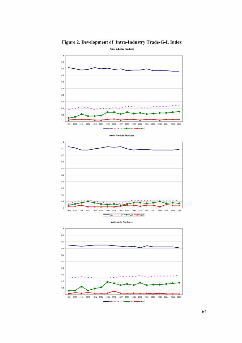
64
Figure 2. Development of Intra-Industry Trade-G-L Index Auto-Industry Products
0
0.1
0.2
0.3
0.4
0.5
0.6
0.7
0.8
0.9
1
1989 1990 1991 1992 1993 1994 1995 1996 1997 1998 1999 2000 2001 2002 2003 2004 2005 2006
Inter IIT VIIT HIIT
Motor Vehicle Products
0
0.1
0.2
0.3
0.4
0.5
0.6
0.7
0.8
0.9
1
1989 1990 1991 1992 1993 1994 1995 1996 1997 1998 1999 2000 2001 2002 2003 2004 2005 2006
Inter IIT VIIT HIIT Auto-parts Products
0
0.1
0.2
0.3
0.4
0.5
0.6
0.7
0.8
0.9
1
1989 1990 1991 1992 1993 1994 1995 1996 1997 1998 1999 2000 2001 2002 2003 2004 2005 2006
Inter IIT VIIT HIIT

65
Figure 3. Development of Intra-Industry Trade-Decomposition Method Auto-Industry Products
0
0.1
0.2
0.3
0.4
0.5
0.6
0.7
0.8
0.9
1
1989 1990 1991 1992 1993 1994 1995 1996 1997 1998 1999 2000 2001 2002 2003 2004 2005 2006
One way TWT TWTV TWTH
Motor Vehicle Products
0
0.1
0.2
0.3
0.4
0.5
0.6
0.7
0.8
0.9
1
1989 1990 1991 1992 1993 1994 1995 1996 1997 1998 1999 2000 2001 2002 2003 2004 2005 2006
One way TWT TWTV TWTH Auto-parts Products
0
0.1
0.2
0.3
0.4
0.5
0.6
0.7
0.8
0.9
1
1989 1990 1991 1992 1993 1994 1995 1996 1997 1998 1999 2000 2001 2002 2003 2004 2005 2006
One way TWT TWTV TWTH

66
Table 1. The U.S. Auto-Parts Trade by Countries (Values is in Millions of $)
1989 2006 Exports Imports Exports Imports Countries
Value Share Value Share Value Share Value Share Australia 357.9 0.0210 63.7 0.0020 874.3 0.0164 185.0 0.0020 Austria 35.5 0.0021 74.3 0.0024 887.7 0.0166 355.5 0.0038 Belgium 195.7 0.0115 107.9 0.0034 394.5 0.0074 136.0 0.0015 Brazil 141.7 0.0083 840.3 0.0266 601.2 0.0113 2,002.5 0.0216 Canada 9,828.5 0.5781 9,387.5 0.2973 31,895.7 0.5970 17,274.5 0.1861 China 23.7 0.0014 59.5 0.0019 815.3 0.0153 6,147.4 0.0662 Denmark 7.6 0.0004 9.4 0.0003 17.4 0.0003 30.2 0.0003 Finland 16.2 0.0010 10.0 0.0003 42.2 0.0008 52.8 0.0006 France 133.0 0.0078 776.6 0.0246 657.0 0.0123 1,115.4 0.0120 Germany 410.9 0.0242 1,939.7 0.0614 1,591.2 0.0298 6,582.2 0.0709 Hong Kong 24.0 0.0014 166.2 0.0053 102.8 0.0019 118.0 0.0013 Ireland 8.1 0.0005 4.3 0.0001 39.7 0.0007 19.7 0.0002 Italy 78.5 0.0046 432.2 0.0137 139.2 0.0026 723.9 0.0078 Japan 618.4 0.0364 10,954.8 0.3469 1,747.7 0.0327 13,255.8 0.1428 Korea 158.9 0.0093 696.3 0.0221 570.1 0.0107 3,136.3 0.0338 Malaysia 4.5 0.0003 12.4 0.0004 25.9 0.0005 207.4 0.0022 Mexico 3,310.4 0.1947 4,390.3 0.1390 12,795.1 0.2395 23,688.2 0.2552 Netherlands 121.7 0.0072 49.6 0.0016 356.4 0.0067 90.9 0.0010 New Zealand 18.1 0.0011 24.2 0.0008 30.5 0.0006 13.0 0.0001 Norway 10.9 0.0006 7.0 0.0002 28.9 0.0005 27.2 0.0003 Philippines 26.9 0.0016 165.0 0.0052 115.6 0.0022 498.7 0.0054 Poland 2.8 0.0002 3.9 0.0001 47.5 0.0009 93.7 0.0010 Portugal 5.1 0.0003 17.0 0.0005 18.8 0.0004 91.5 0.0010 Singapore 83.0 0.0049 121.5 0.0038 238.5 0.0045 78.9 0.0008 Spain 28.3 0.0017 353.7 0.0112 277.9 0.0052 403.4 0.0043 Sweden 102.9 0.0061 124.3 0.0039 197.8 0.0037 550.2 0.0059 Thailand 37.1 0.0022 113.8 0.0036 78.7 0.0015 888.3 0.0096 Turkey 30.7 0.0018 11.1 0.0004 41.6 0.0008 91.0 0.0010 United Kingdom 447.1 0.0263 660.2 0.0209 871.5 0.0163 938.6 0.0101 Core 12,526.3 0.7367 25,267.0 0.8002 40,390.9 0.7560 41,951.1 0.4519 Periphery 3,741.7 0.2200 6,309.7 0.1998 15,109.7 0.2828 36,845.1 0.3969 Source: Authors’ own calculations.

67
Table 2. Auto-Parts Trade by Product Groups (Values is in Millions of $), 1989-2006. 1989 2006
Exports Imports Exports Imports Product Groups Value Share Value Share Value Share Value Share
Bodies and Parts 3,759.30 0.22 4,568.97 0.14 15,185.75 0.26 14,879.59 0.18 Chassis and Drivetrain Parts 7,760.87 0.45 12,649.52 0.39 22,559.31 0.38 28,751.11 0.35 Electrical and Electric Components 2,077.29 0.12 5,401.43 0.17 5,522.29 0.09 15,380.71 0.19 Engines and Parts 2,486.05 0.14 6,427.90 0.20 11,180.60 0.19 16,794.56 0.21 Tires and Tubes 672.57 0.04 2,536.73 0.08 2,643.78 0.05 3,430.52 0.04 Miscellaneous Parts 490.68 0.03 741.28 0.02 1,553.72 0.03 2,140.17 0.03 Source: Authors’ own calculations. Table 3. Top 5 Import Sources of the U.S. Auto-Parts Industry in 2006 (Values is in Millions of $) Product Groups Country-I Country-II Country-
III Country-
IV Country-V World
Mexico Canada Japan Germany China Bodies and Parts 5,316.47 4,841.41 1,256.05 1,081.17 757.05 14,879.59 Canada Japan Mexico China Germany Chassis and
Drivetrain Parts 6,901.31 6,450.29 5,490.59 2,377.01 2,106.45 28,751.11 Mexico Japan China Taiwan Philippines Electrical and
Electric Components
8,398.98 1,915.81 1,519.75 456.89 455.81 15,380.71
Canada Mexico Japan Germany Brazil Engines and Parts 3,920.97 3,884.38 2,849.97 2,731.94 1,064.63 16,794.56
China Canada Japan Korea Thailand Tires and Tubes 872.97 869.45 569.33 278.76 192.23 3,430.52 Mexico Canada China Japan Germany Miscellaneous
Parts 515.71 418.66 313.05 214.34 172.21 2,140.17 Source: Authors’ own calculations. Table 4. Top 5 Export Destinations of the U.S. Auto-Parts Industry in 2006 (Values is in Millions of $) Product Groups
Country-I Country-II Country-III Country-IV Country-V World
Canada Mexico Germany Japan Austria Bodies and Parts 8,839.92 4,219.88 500.90 461.46 334.85 15,185.75
Canada Mexico Japan Germany China Chassis and Drivetrain Parts 12,543.81 4,380.15 894.60 815.73 547.96 22,559.31
Canada Mexico Japan Germany France Electrical and Electric Components
3,151.07 1,338.14 126.61 100.78 96.28 5,522.28
Canada Mexico UK Australia Japan Engines and Parts 6,561.00 2,547.13 308.72 250.73 243.33 11,180.6
Canada Mexico Australia Germany Netherlands Tires and Tubes 1,342.52 737.83 111.12 89.96 64.21 1,553.72 Canada Mexico Australia Austria Germany Miscellaneous
Parts 1,052.21 211.70 52.55 42.83 32.89 2,643.78 Source: Authors’ own calculations.
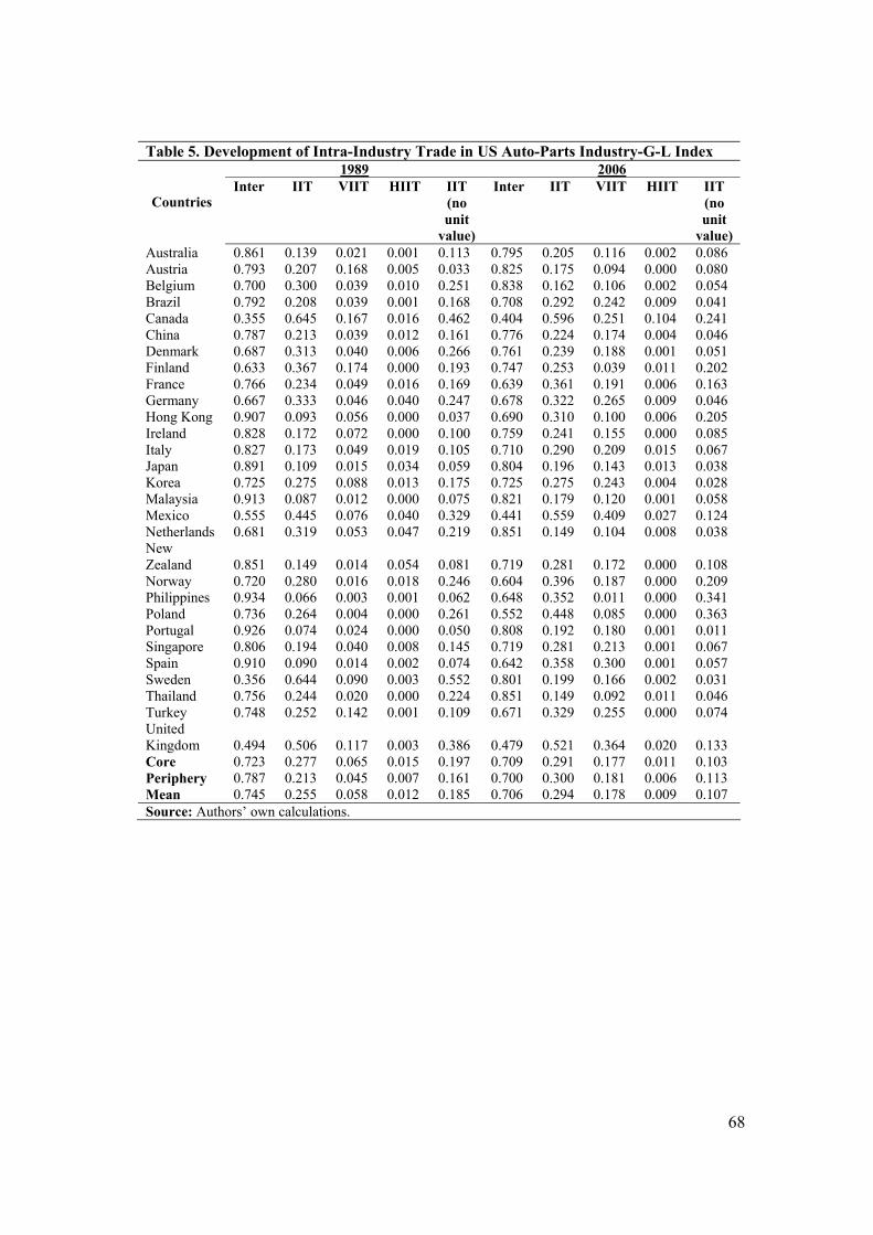
68
Table 5. Development of Intra-Industry Trade in US Auto-Parts Industry-G-L Index 1989 2006
Countries Inter IIT VIIT HIIT IIT
(no unit
value)
Inter IIT VIIT HIIT IIT (no unit
value) Australia 0.861 0.139 0.021 0.001 0.113 0.795 0.205 0.116 0.002 0.086 Austria 0.793 0.207 0.168 0.005 0.033 0.825 0.175 0.094 0.000 0.080 Belgium 0.700 0.300 0.039 0.010 0.251 0.838 0.162 0.106 0.002 0.054 Brazil 0.792 0.208 0.039 0.001 0.168 0.708 0.292 0.242 0.009 0.041 Canada 0.355 0.645 0.167 0.016 0.462 0.404 0.596 0.251 0.104 0.241 China 0.787 0.213 0.039 0.012 0.161 0.776 0.224 0.174 0.004 0.046 Denmark 0.687 0.313 0.040 0.006 0.266 0.761 0.239 0.188 0.001 0.051 Finland 0.633 0.367 0.174 0.000 0.193 0.747 0.253 0.039 0.011 0.202 France 0.766 0.234 0.049 0.016 0.169 0.639 0.361 0.191 0.006 0.163 Germany 0.667 0.333 0.046 0.040 0.247 0.678 0.322 0.265 0.009 0.046 Hong Kong 0.907 0.093 0.056 0.000 0.037 0.690 0.310 0.100 0.006 0.205 Ireland 0.828 0.172 0.072 0.000 0.100 0.759 0.241 0.155 0.000 0.085 Italy 0.827 0.173 0.049 0.019 0.105 0.710 0.290 0.209 0.015 0.067 Japan 0.891 0.109 0.015 0.034 0.059 0.804 0.196 0.143 0.013 0.038 Korea 0.725 0.275 0.088 0.013 0.175 0.725 0.275 0.243 0.004 0.028 Malaysia 0.913 0.087 0.012 0.000 0.075 0.821 0.179 0.120 0.001 0.058 Mexico 0.555 0.445 0.076 0.040 0.329 0.441 0.559 0.409 0.027 0.124 Netherlands 0.681 0.319 0.053 0.047 0.219 0.851 0.149 0.104 0.008 0.038 New Zealand 0.851 0.149 0.014 0.054 0.081 0.719 0.281 0.172 0.000 0.108 Norway 0.720 0.280 0.016 0.018 0.246 0.604 0.396 0.187 0.000 0.209 Philippines 0.934 0.066 0.003 0.001 0.062 0.648 0.352 0.011 0.000 0.341 Poland 0.736 0.264 0.004 0.000 0.261 0.552 0.448 0.085 0.000 0.363 Portugal 0.926 0.074 0.024 0.000 0.050 0.808 0.192 0.180 0.001 0.011 Singapore 0.806 0.194 0.040 0.008 0.145 0.719 0.281 0.213 0.001 0.067 Spain 0.910 0.090 0.014 0.002 0.074 0.642 0.358 0.300 0.001 0.057 Sweden 0.356 0.644 0.090 0.003 0.552 0.801 0.199 0.166 0.002 0.031 Thailand 0.756 0.244 0.020 0.000 0.224 0.851 0.149 0.092 0.011 0.046 Turkey 0.748 0.252 0.142 0.001 0.109 0.671 0.329 0.255 0.000 0.074 United Kingdom 0.494 0.506 0.117 0.003 0.386 0.479 0.521 0.364 0.020 0.133 Core 0.723 0.277 0.065 0.015 0.197 0.709 0.291 0.177 0.011 0.103 Periphery 0.787 0.213 0.045 0.007 0.161 0.700 0.300 0.181 0.006 0.113 Mean 0.745 0.255 0.058 0.012 0.185 0.706 0.294 0.178 0.009 0.107 Source: Authors’ own calculations.

69
Table 6. Development of Intra-Industry Trade in US Auto-Parts Industry- Decomposition Method
1989 2006
Countries One-way
TWT TWTV TWTH Not Classified
TWT
One-way
TWT TWTV TWTH Not Classified
TWT Australia 0.841 0.159 0.029 0.000 0.129 0.735 0.265 0.156 0.001 0.107 Austria 0.447 0.553 0.501 0.023 0.029 0.602 0.398 0.342 0.000 0.056 Belgium 0.543 0.457 0.064 0.015 0.378 0.595 0.405 0.316 0.002 0.087 Brazil 0.741 0.259 0.039 0.000 0.220 0.476 0.524 0.463 0.001 0.060 Canada 0.072 0.928 0.207 0.028 0.693 0.175 0.825 0.379 0.142 0.305 China 0.648 0.352 0.063 0.014 0.274 0.616 0.384 0.325 0.005 0.055 Denmark 0.660 0.340 0.030 0.006 0.304 0.601 0.399 0.294 0.003 0.102 Finland 0.342 0.658 0.188 0.000 0.470 0.546 0.454 0.031 0.031 0.392 France 0.635 0.365 0.070 0.004 0.291 0.457 0.543 0.306 0.013 0.224 Germany 0.473 0.527 0.084 0.072 0.372 0.431 0.569 0.456 0.020 0.092 Hong Kong 0.897 0.103 0.039 0.000 0.064 0.361 0.639 0.244 0.006 0.388 Ireland 0.699 0.301 0.139 0.000 0.162 0.487 0.513 0.229 0.000 0.283 Italy 0.676 0.324 0.090 0.002 0.232 0.543 0.457 0.333 0.023 0.101 Japan 0.883 0.117 0.019 0.051 0.047 0.608 0.392 0.285 0.043 0.064 Korea 0.585 0.415 0.163 0.015 0.237 0.457 0.543 0.498 0.002 0.042 Malaysia 0.850 0.150 0.014 0.000 0.135 0.726 0.274 0.166 0.002 0.107 Mexico 0.310 0.690 0.124 0.067 0.499 0.210 0.790 0.534 0.069 0.187 Netherlands 0.343 0.657 0.100 0.066 0.491 0.700 0.300 0.221 0.006 0.073 New Zealand 0.830 0.170 0.036 0.073 0.061 0.555 0.445 0.289 0.000 0.156 Norway 0.540 0.460 0.020 0.060 0.380 0.431 0.569 0.205 0.000 0.364 Philippines 0.988 0.012 0.001 0.001 0.010 0.170 0.830 0.018 0.000 0.813 Poland 0.640 0.360 0.001 0.000 0.359 0.450 0.550 0.115 0.000 0.435 Portugal 0.982 0.018 0.010 0.000 0.007 0.553 0.447 0.422 0.001 0.025 Singapore 0.757 0.243 0.070 0.005 0.168 0.554 0.446 0.353 0.004 0.089 Spain 0.937 0.063 0.022 0.003 0.038 0.415 0.585 0.510 0.002 0.074 Sweden 0.189 0.811 0.114 0.007 0.689 0.513 0.487 0.416 0.001 0.069 Thailand 0.252 0.748 0.068 0.000 0.680 0.698 0.302 0.138 0.019 0.145 Turkey 0.536 0.464 0.171 0.004 0.289 0.470 0.530 0.425 0.000 0.105 United Kingdom 0.074 0.926 0.366 0.004 0.556 0.188 0.812 0.576 0.042 0.195 Core 0.570 0.430 0.115 0.022 0.292 0.500 0.500 0.313 0.018 0.170 Periphery 0.653 0.347 0.066 0.010 0.271 0.483 0.517 0.310 0.010 0.197 Mean 0.599 0.401 0.098 0.018 0.285 0.494 0.506 0.312 0.015 0.179 Source: Authors’ own calculations.

70
Table 7. Development of Intra-Industry Trade in US Auto-Parts Industry by Product Groups – G-L Index
1989 2006 Product Groups Inter IIT VIIT HIIT Inter IIT VIIT HIIT
Bodies and Parts 0.637 0.363 0.113 0.000 0.389 0.611 0.537 0.009 Chassis and Drivetrain Parts 0.517 0.483 0.002 0.002 0.452 0.548 0.271 0.004 Electrical and Electric Components 0.679 0.321 0.059 0.005 0.791 0.209 0.080 0.016 Engines and Parts 0.629 0.371 0.348 0.002 0.630 0.370 0.158 0.182 Tires and Tubes 0.627 0.373 0.158 0.215 0.750 0.250 0.243 0.006 Miscellaneous Parts 0.511 0.489 0.022 0.005 0.654 0.346 0.166 0.006 Source: Authors’ own calculations. Table 8. Development of Intra-Industry Trade in US Auto-Parts Industry by Product Groups- Decomposition Method
1989 2006 Product Groups One-way TWT TWTV TWTH One-way TWT TWTV TWTH
Bodies and Parts 0.369 0.631 0.160 0.032 0.151 0.849 0.718 0.023 Chassis and Drivetrain Parts 0.331 0.669 0.003 0.002 0.233 0.767 0.406 0.007 Electrical and Electric Components 0.513 0.487 0.066 0.006 0.631 0.369 0.140 0.072 Engines and Parts 0.511 0.489 0.421 0.031 0.371 0.629 0.287 0.292 Tires and Tubes 0.370 0.630 0.233 0.397 0.641 0.359 0.356 0.003 Miscellaneous Parts 0.306 0.694 0.048 0.012 0.311 0.689 0.384 0.020 Source: Authors’ own calculations.

71
Table 9. Determinants of Vertical Intra-Industry Trade in the U.S. Auto-Parts Industry, 1989-2006 Independent Variables Pooled OLS Fixed Effects FGLS PCSE
ktGDP 6.751 (4.11)***
22.424 (8.73) ***
1.344 (3.96) ***
6.751 (5.32) ***
ktDGDP 3.191 (3.53) ***
12.179 (8.39) ***
0.405 (1.68) *
3.191 (4.00) ***
ktDPGDP -0.051 (-0.74)
-0.086 (-1.27)
0.287 (3.79) ***
-0.051 (-1.26)
ktFDI 0.195 (4.23) ***
0.087 (1.85) *
0.244 (4.79) ***
0.195 (7.57) ***
kDIST -0.242 (-2.56) **
-0.215 (-2.35) **
-0.351 (-3.80) ***
-0.242 (-4.43) ***
ktEXCH 0.036 (1.29)
0.059 (2.22) **
0.058 (2.39) **
0.036 (2.71) ***
ktNAFTA 0.243 (1.19)
0.296 (1.51)
0.046 (0.34)
0.243 (2.24) **
Constant -290.784 (-4.00) ***
-1017.049 (-8.67) ***
-55.047 (-6.87) ***
-290.784 (-4.86) ***
R-squared 0.29 0.06 0.29 F-statistics 23.96*** 34.69*** Wald statistic: 2χ (7) 263.72*** 29174.05***
Wooldridge test for autocorrelation: F (1,28)
10.70***
LR-test for heteroscedasticity: 2χ (28)
177.20***
Chow test (43,415) 6.43*** Breusch-Pagan LM test for random effects: 2χ (1)
219.85***
Hausman specification test: 2χ (6)
3.40
# of groups 29 29 29 29 # of observations 466 466 466 466 Notes: The dependent variable is the logit transformation of ktVIIT , Grubel-Lloyd index in vertically differentiated products. Heteroskedasticity-consistent t-statistics (White-Newey) are reported in the first and second columns. ***, **, * indicate statistical significance at 1%, 5 %, and 10% levels, respectively.

72
Table 10: Determinants of Two-Way Trade in Vertically Differentiated Goods in the U.S. Auto-Parts Industry, 1989-2006 Independent Variables Pooled OLS Fixed Effects FGLS PCSE
ktGDP 5.339 (2.55)**
24.704 (7.55) ***
1.176 (3.73) ***
5.339 (3.77)***
ktDGDP 2.213 (1.88)*
13.337 (6.97) ***
0.101 (0.45)
2.213 (2.60) ***
ktDPGDP -0.102 (-1.26)
-0.146 (-1.81) *
0.191 (3.04) ***
-0.102 (-1.66) *
ktFDI 0.295 (5.47) ***
0.167 (3.08) **
0.369 (8.40) ***
0.295 (9.69) ***
kDIST -0.395 (-3.13) ***
-0.343 (-2.92) ***
-0.553 (-5.36) ***
-0.395 (-3.74) ***
ktEXCH 0.057 (1.57)
0.085 (2.49) * *
0.071 (2.81) ***
0.057 (3.33) ***
ktNAFTA -0.079 (-0.28)
0.039 (0.16)
-0.120 (-0.76)
-0.079 (-0.42)
Constant -219.617 (-2.35)**
-116.43 (-7.37) ***
-38.752 (-5.26) ***
-219.617 (-3.34) ***
R-squared 0.29 0.10 0.29 F-statistics 25.63*** 34.12*** Wald statistic: 2χ (7) 428.55*** 4547.53***
Wooldridge test for autocorrelation: F (1,28)
2.134
LR-test for heteroscedasticity: 2χ (28)
161.21***
Chow test (43,415) 5.58*** Breusch-Pagan LM test for random effects: 2χ (1)
201.65***
Hausman specification test: 2χ (6)
1.60
# of groups 29 29 29 29 # of observations 466 466 466 466 Note: The dependent variable is the logit transformation of ktTWTV , the share of two-way trade in vertically differentiated products. Heteroskedasticity-consistent t-statistics (White-Newey) are reported in the first and second columns. ***, **, * indicate statistical significance at 1%, 5 %, and 10% levels, respectively.