Embed Size (px)
Citation preview
VERTICAL MERGERS AND THE MARKET VALUATION OF THE
BENEFITS OF VERTICAL INTEGRATION
This Version: October 2008
By:
Simi Kedia* S. Abraham Ravid** and Vicente Pons***
JEL G34, L1
*Rutgers Business School, Newark, NJ 07102,
** The Wharton School, University of Pennsylvania, 2439 Steinberg Hall-Dietrich Hall
3620 Locust Walk, Philadelphia, PA 19104-6367, Phone: 215-898-7617; Email: [email protected] and
Rutgers Business School.
*** Renaissance Capital, London, England.
We thank brown bag seminar participants at NYU and seminar participants at Binghamton
University and INSEAD for many useful comments. The usual disclaimer applies.
2
ABSTRACT:
This paper explores the market reaction to vertical mergers and incorporates into the analysis
predictions based on I/O theories.
We develop a classification to separate the various types of mergers, and focus on the determinants
and wealth impacts of vertical mergers over the period 1979-2002. Abnormal returns for vertical
merger announcements are positive until 1996, and turn negative afterwards. Acquirers suffer most
of the losses. We present and test several hypotheses based upon some well known I/O theories of
vertical integration. We find support for the most fundamental insight in the I/O literature, namely,
that vertical mergers generate most value when undertaken in imperfectly competitive markets and
when firms have to invest in specialized assets making market exchanges difficult. There is little
evidence to support the view that information based contracting problems or price uncertainty, at
least as captured in this paper, generate a value maximizing rationale for vertical integration.
However, we show that informational asymmetries can increase the value of horizontal mergers.
3
I. INTRODUCTION.
If markets were competitive, with no frictions, then transactions between firms could be efficiently
executed with arm’s length contracts. However, market frictions can lead to a rationale for integration
and mergers. This insight can be traced back to Stigler (1951), and its implications are explored in
numerous subsequent studies. In this paper, we use some new tools in order to classify mergers into
vertical, horizontal, and conglomerate deals. We then compare the market reaction to vertical
mergers’ announcements to the reaction to other types of mergers. We also link our findings
empirically to the large I/O literature on vertical integration. This is one of the a few papers focusing
on vertical and horizontal mergers. Conglomerate mergers, on the other hand, have received much
more attention in numerous studies, published in the 1990’s and early 21st century.
A significant obstacle to the study of vertical mergers had been the identification of vertically
related transactions. Horizontal mergers are more easily classified and have been studied by Eckbo
(1983,1985) and more recently by Fee and Thomas (2004), Shahrur (2005) and Gugler and Siebert
(2007). In the only study, to our knowledge, of vertical mergers, Fan and Goyal (2006) use the
Benchmark Input Output tables compiled by Bureau of Economic Analysis to develop a classification
system for vertical deals. Our measures are similar to the ones they use. However, we extend the Fan
and Goyal (2006) analysis in several important ways. Fan and Goyal (2006) find that, on average,
vertical mergers are associated with significant positive wealth effects. These positive synergies stand
in contrast to the vast literature suggesting that unrelated, or conglomerate mergers, destroy value.1
Our sample includes all completed mergers over the period 1979 to 2002. We find little evidence
to support the view that vertical mergers create value. However, value creation (destruction) by
vertical mergers changes over time. On average, transactions until 1996, the sample period studied by
Fan and Goyal (2006), indeed had positive announcement effects. However, later vertical mergers are
associated with significant losses. Mergers of all types performed worse in the late 1990’s and early
2000’s, but value destruction is greatest for vertical mergers2. We also extend the Fan and Goyal
(2006) analysis by considering acquirers and targets separately, which provides interesting insights,
and most importantly, we empirically explore the implications of various I/O theories of vertical
integration in the context of merger transactions.
1 Berger and Ofek (1995) and Lang and Stulz (1995) were the first to find that conglomerates trade at a discount. There are several papers that examine the source of this discount like Servaes Rajan and Zingales(2000), and Shoar (2002) among others. Further work by Maksimovic and Phillips (2002), Campa and Kedia (2002) and Villalonga (2004) argues that the observed diversification discount does not imply that diversifying in by itself destroys value. 2 This is consistent with other work. Moeller et al. (2005) document “wealth destruction on a massive scale” between1998-2001. The idea of merger waves with different characteristics is explored in Rhodes Kroft and Viswanathan (2004) and Qiu and Zhou (2007) among others.
4
A large body of I/O literature, discussed in detail in the next section, shows that in the presence of
imperfect competition, firms can generate value by vertical integration. Although the details of the
outcome vary across these papers depending on assumptions and specifications, these models
collectively suggest that gains may arise from the possibility of rationing inputs, shutting out
competitors and from price discrimination as well as the elimination of double marginalization (see
Perry, 1989).
We cannot test dozens of theories directly, however, we can test the necessary condition for these
theories to hold, namely, whether or not a non-competitive environment leads, on average to “better”
vertical mergers. If this is not the case, one can question the validity of the theoretical view of vertical
integration. We can also see how the three types of mergers (horizontal, vertical and conglomerate)
fare in non-competitive environments.
We find that vertical deals in non-competitive environments are associated with higher returns
relative to other vertical deals. This is not necessarily true for horizontal or conglomerate mergers. In
order to test this premise further, we look at competitors of the merged companies. We find, that, as
predicted in much of the I/O literature, vertical mergers are detrimental to competitors of the target
and of the acquirer.
Market power based theories of vertical integration are divided as to the benefits or costs to
consumers of such integration (see Lafontaine and Slade, 2007, Salinger, 1988, Hart and Tirole, 1990,
Riordan, 1998, Chen and Riordan , 2007, De Fontenay and Gans, 2007 to name a few). Our results
address this question to some extent, although a complete answer must include consumer surplus and
similar measures which are beyond the scope of this investigation.
Another potential benefit of vertical integration may arise in the presence of asset specificity.
Williamson (1983) is the first to discuss this issue. Perry (1989), among others, shows that when firms
need to invest in assets that are specialized and market exchanges are difficult, vertical integration may
lead to efficient investment. In line with Caves and Bradburd (1988) we use R&D expenditure to
capture asset specificity, and find that vertical deals when both the target and acquirer are R&D
intensive, are associated with higher total returns. These gains are seen only in vertical deals and not
in horizontal or conglomerate mergers3.
Grossman and Hart (1986) show that with incomplete contracts vertical integration may provide
better investment incentives. The empirical I/O evidence on this matter, which is all industry
3 There is a variety of other measures used for asset specificity in I/O studies (see Lafontaine and Slade, 2007). However, the vast majority of these studies focused on one industry and thus measures could be more industry specific.
5
specific, is mixed (see the survey of Lafontaine and Slade, 2007). We use analyst coverage to proxy for
information opacity and the difficulty of arm’s length contracting. However, we find no evidence to
support the view that vertical integration leads to higher returns in the presence of information
problems. Horizontal mergers, on the other hand, do seem to be motivated by information
asymmetries. Lastly, we test to see if in the presence of price uncertainty vertical integration may be
associated with efficient production decisions and therefore higher value. We use the volatility of the
producer price index in the acquirer and target industry to capture price uncertainty and find no effect
on the value generated from vertical or any other type of merger.
In summary, we find that unlike horizontal deals, vertical transactions do not on average, create
positive wealth effects for shareholders. Vertical mergers, however, appear to generate the greatest
returns when dominant firms integrate and are able to shut out or discriminate against rival firms.
There is weak evidence to suggest that vertical integration generates value when assets are specialized
and no evidence that information problems or price uncertainty present opportunities for value
maximizing vertical integration.
This paper complements the vast empirical I/O literature on vertical integration. Typically such
papers (for a fairly large scale survey see Lafonataine and Slade , 2007) consider the probability of
vertical integration in the context of one specific industry.
We consider the market reaction to merger announcements. Thus we look at factors common to all
industries, and naturally, our perspective is the market valuation of vertical merger gains.
The rest of the paper is organized as follows. The next section discusses the theoretical rationales for
value maximizing vertical integration and develops our hypotheses. Section 3 develops our measures
of vertical integration, Section 4 describes the data and discusses wealth effects of mergers, Section 5
examines the various rationales for vertical mergers. Section 6 concludes.
.
II. VALUE DETERMINANTS OF VERTICAL MERGERS AND HYPOTHESIS
In this section, we briefly review the literature that documents theoretically and empirically the value
of vertical integration.4 This will lead to our testable hypotheses.
The vast majority of the empirical I/O literature covers one industry, and sometimes includes
industry specific proxies, such as paper capacity for the pulp and paper industry (see Ohanian, 1994)
4 We will not be able to address every contribution- a recent survey of the empirical work alone (Lafontaine and Slade, 2007) has a reference list of over 150 papers.
6
or the number of rooms for the hospitality industry (See Kehoe, 1996). Our work focuses on some
general properties which may make vertical integration advantageous and suggest proxies which cut
across industries5.
The theory of vertical integration can be traced back to Stigler (1951) and in a more specific context,
to Williamson (1971). Several papers, starting with Stigler (1951) point out that in the presence of
non-competitive markets vertical integration may be beneficial. Many theoretical studies examine the
role of vertical integration when there is a dominant firm in the industry (See Riordan (1998),
Williamson (1971) and Salinger (1988)).
Riordan (1998), for example, shows that if there is a dominant firm in an industry with a cost
advantage relative to a competitive fringe, then it will tend to vertically merge backwards. This
increases the dominant firm’s capacity at the expense of the fringe. Both output and input prices
increase in the degree of vertical integration. Although a vertical merger may lead to a decrease in
profits for some of the firms in the fringe, profits increase for the dominant firm.
Other papers, such as Ordover, Saloner and Salop (1990)) and Tirole et al. (1990), show that vertical
integration may be value maximizing if it raises rival’s costs. In an oligopolistic setting, a firm may
buy its suppliers and thus shut out rival buyers altogether, or increase their costs. In a similar vein,
Hart and Tirole (1990) note the importance of “market foreclosure” in making vertical mergers a
relevant and value maximizing proposition. Chen and Rirordan (2007) point out that, again, in a non-
competitive environment, vertically integrated firms can use exclusive contracts to exclude an equally
efficient upstream firm and effect a downstream cartelization. De Fontenay and Gans (2007) compare
the case of an upstream monopoly to a case where few competitors exist and focus on incentives
created by the outcome of a possible bargaining process between upstream and downstream firms.
(See also Klein and Murphy , 1997).
The details of the outcome vary across models and depend on assumptions related to demand
functions (Dixit , 1983) or the specification of downstream competition and existing externalities (See
deFontenay and Gans , 2005, Chen and Riordan, 2007). The efficiency consequences are also
debated. However, collectively, these models suggest that non-competitive markets with the
possibility of rationing, shutting out competitors, elimination of externalities, possibility of exclusive
contracts and price discrimination may generate at least a private rationale for vertical integration.
(See also McNicol (1975), or Perry (1980), and a survey by Perry (1989)). The specific predictions are
5 Similarly, in a wide ranging study which covers vertical integration in 93 countries, Acemoglu et al. (2007) focus on the few variables which are general and vary from country to country.
7
often contradictory and relate to consumer welfare. However, we can test the following proposition-
vertical mergers, on average, should be more successful if the necessary conditions that underlie much
of the theoretical I/O literature hold. In other words, if vertical mergers do not “work” in a non-
competitive environment, it will cast some doubt on quite a few of the I/O conjectures. It is an
empirical question whether or not this rationale is stronger for vertical or horizontal mergers. Fee and
Thomas (2004) and Shahrur (2005) point out that in the case of horizontal mergers, efficiencies can
lead to the observed beneficial effect, even in the case of competitive industries. Similarly, Gugler and
Siebert (2007) show that for the semiconductor industry, and in particular for the memory and micro-
components market, horizontal mergers and research joint ventures lead to an increased market share
for the combined firm, which is consistent with efficiency gains. We focus on vertical mergers, but
since we do classify mergers as horizontal, vertical and other, we can try to some extent to verify the
findings in the horizontal mergers’ literature as well.
The discussion in the previous paragraph of market structure and mergers, naturally leads to our first
hypothesis:
H1: Vertical mergers should be more successful in a non-competitive environment.
The presence of transaction costs may affect the optimality of vertical integration as pointed out by
Williamson (1975), Klein et al. (1978), Williamson and Riordan (1985), and Perry (1989). In particular,
when firms need to invest in assets that are specialized, and when the market exchange of these assets
is costly, vertical integration may align the incentives of the parties involved and may lead to efficient
investment (see also Joskow, 1993); This insight is nicely stated in Caves and Bradburd (1988, p.268)
“The chief empirical predictors of vertical integration coming from the transaction cost model are
small numbers of transactors on both sides of the market ex-ante and the prevalence of transaction
specific assets and switching costs that create ex post lock in problems with arm-length transactions”.
In other words, we would expect mergers, which create “internal markets” to work better for
companies with high asset specificity. Asset specificity in that sense can be related to dedicated assets,
geographical distance or human capital or it can be more general.
We should note that most of the numerous empirical I/O studies (most of them industry specific)
find that asset specificity increases vertical integration. Spiller (1985), for example, considers vertical
mergers and uses as an independent variable the distance between plants, which proxies for specificity
of assets. He finds that distance negatively affects stock returns in mergers. Naturally the analysis is
much different than ours. Levy (1985) finds no relation between distance and returns but finds that
8
research and development intensity, (another measure of asset specificity), affects returns.6 Masten et
al. (1989) show that measures of human capital and asset specificity increase the proportion of parts
in the auto industry produced by the manufacturer, which their measure of integration. Lieberman
(1991) studies plant level and firm level integration in the Chemical industry and also concludes that
the probability of vertical integration increases with asset specificity and input variability. Caves and
Bradburd (1988) show that R&D intensity significantly affects the probability of mergers. Masten et
al. (1989) Anderson and Scmittlein (1984) are among the other studies which use R&D as a proxy for
asset specificity.7 We follow this body of work and use R&D intensity to capture asset specificity and
study its role in generating value through vertical integration by formulating our second hypothesis:
H2: Vertical mergers should be associated with higher returns when the target and/or the acquirer are R&D intensive.
Some of the studies of vertical integration focus on incomplete contracts and the incentives they
create. If contracts are hard to specify, enforce, and monitor on the outside, and it is cheaper to
monitor and contract within the firm, then vertical integration can increase efficiency. Grossman and
Hart (1986) suggest that investment incentives may differ as a result of the allocation of control rights
ex-post, and thus, depending on relatedness, vertical integration may provide the correct investment
incentives. A similar framework underlies Tirole (1986) and Hart and Moore (1988). Klein. Hughes
and Kao (2001) model more directly the advantage gained by information sharing between upstream
and downstream firms in non-competitive markets. If vertical integration is an efficient tool in a
world of asymmetric information and incomplete contracts, then vertical mergers should be
associated with higher returns when contracting is harder. We use the degree of information opacity
of the target and acquiring firm to capture instances where arm length contracting is less effective and
formulate our next hypothesis.
H3: Vertical mergers should be associated with higher returns when there is less public information available about the
target and the acquirer.
6 Quite a few papers (see the survey by Lafontaine and Slade, 2007) use geographical measures to proxy for monitoring cost in empirical studies. Uysal Kedia and Panchapagesan (2008) examine distance between acquirer and target and find that though nearby deals have higher returns relative to distant deals, this relation is the same for all types of mergers. We therefore do not consider distance in our paper. 7 Weiss (1992) using an interesting research design, considers the correlation between abnormal returns of vertically merging firms in order to account for firms specific capital. However, he has only 18 daily cases and 11 monthly cases over 25 years.
9
Another rationale for vertical integration, which has been used often in the popular press, is the presence of
supply price uncertainty. For example, one of the benefits cited for the vertical merger between Disney and
ABC was that it allowed ABC to have greater control over the content, i.e., the “supply” of TV programming.
Although supply uncertainty affects everybody, its presence may give a rationale for vertical integration if such
integration allows for efficient organization of production or cheaper gathering of information. Several models
discuss various manifestations of this idea. Carlton (1977), suggests that if price uncertainty exists, firms will
charge a premium to account for the possibility of not being able to sell their entire production. If integration
can provide a higher probability of usage, then vertical integration will provide cost savings. More recently,
Baker Gibbons and Murphy (2002) discuss incentives in relational contracts for upstream and downstream
parties. One of their results concerns prices. Low prices create incentives for downstream consumers to renege
on contracts, and similarly, high prices create incentives for upstream producers to renege (result 1, ibid).
Therefore, they conclude that large price dispersion (a big difference between the two outcomes in their model)
encourages firms to seek vertical integration, where temptations to renege on contracts do not exist.
Therefore, we propose:
H4: Vertical mergers should be associated with higher returns when there is greater price uncertainty in the acquirer and
the target industries.
We now proceed to discuss our empirical strategy and our findings.
III. MEASURING VERTICAL INTEGRATION.
The most important empirical barrier to the analysis of vertical merger is the identification of
mergers as horizontal vertical or conglomerate. We follow Fan and Goyal (2006) and Acemoglu et al.
(2007) and use the industry commodity flow information in the Use Table of Benchmark Input-
Output Accounts for the US Economy compiled by the Bureau of Economic Analysis. The Use
Table is a matrix containing the value of commodity flows between each pair of roughly 500 private-
sector intermediate IO industries. If we denote by aij the dollar value of i's output required to
produce industry j’s total output, and then divide aij by the dollar value of industry j’s total output,
then the resulting fraction, which we denote by vij, represents the dollar value of industry i's output
required to produce one dollar’s worth of industry j’s output. For example, if industry j buys from
industry i $500 worth of goods, and then industry j sells $2000 worth of output, vij is 500/2000 =
0.25. We use ( )jiij vv +21
to capture the potential for vertical integration between industries i and j (this
is similar to Fan and Goyal, 2006 and Acemoglu et al., 2007). We use the average of the coefficients

10
for vertical relation as very often industries sell in both directions, and ignoring one direction might
bias our analysis. As the Use tables give flows between IO industries, we convert the acquirer and
target CRSP SIC code to the IO industry codes. We classify mergers as vertically related if the
corresponding vertical coefficient is larger than a certain cutoff. For robustness, we consider 3
alternative cutoffs: 1, 5 and 10 percent8.
A merger transaction is classified as horizontal if both the acquirer and the target are in the same
industry as captured by four-digit CRSP SIC code. If the four-digit SIC industry has a high vertical
relation coefficient with itself, i.e., the industry uses a high fraction of its own output then a
horizontal merger can also be classified as vertically related. We refer to such transactions as mixed
horizontal vertical mergers. Pure horizontal mergers, on the other hand, are mergers classified as
horizontal mergers that are not vertically related. Similarly, pure vertical mergers are those that are
classified as vertically related but are not horizontal. Lastly, if a transaction is neither horizontal nor
vertical, it is classified as a conglomerate merger.
As mentioned above we use three cutoffs, i.e., 1%, 5% and 10% to classify a merger as vertically
related .We also use three different definitions of industry, four digit CRSP SIC codes, two digit SIC
codes as well as Fama French Industry classifications. This analysis leads to nine different
classifications of mergers into the different types i.e., vertical, horizontal, mixed and conglomerate.
We use these different classifications to test the strength and robustness of our results.
IV. MERGER SAMPLE DESCRIPTION AND WEALTH EFFECTS
Our data on acquisitions is from the Securities Data Company's U.S. Mergers and Acquisitions
Database. We select mergers and acquisitions announcements in which both the target and acquirer
are U.S. publicly listed firms; with announcement dates between 1979 and 2002. We consider only
completed deals and exclude LBOs, spinoffs, recapitalizations, self-tender and exchange offers,
repurchases, minority stake purchases, acquisitions of remaining interest, and asset sales. We further
require that acquirer and target’s price data exist in the Center for Research in Security Prices (CRSP)
8 These are similar cutoffs to Fan and Goyal (2006). We should also remember that we are measuring input/output, and thus even a small percentage may indicate a much higher degree of vertical integration.
11
and that we are able to calculate the vertically related coefficient. Our final sample consists of 1692
transactions.
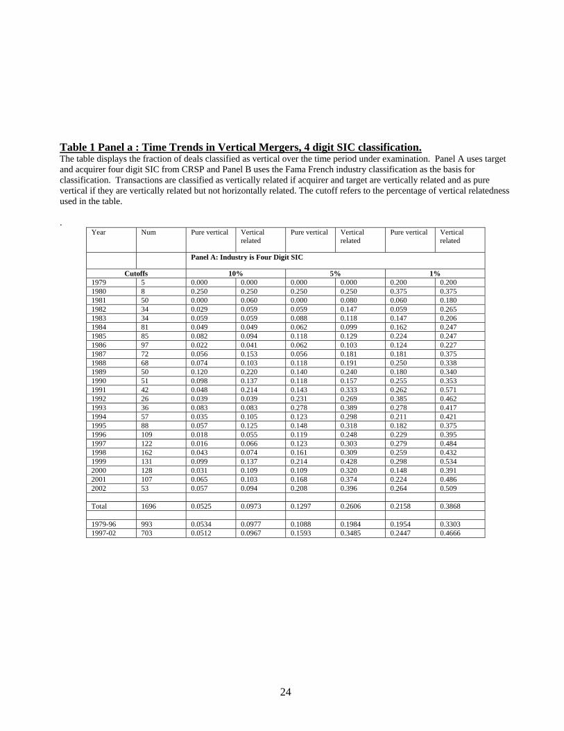
Table I shows the number of acquisitions, as well as the proportion of mergers that are classified as
vertically related over the years. When we use four-digit SIC codes to classify the target and acquirer,
we find that about 9.73% of all deals are vertically related according to the strictest definition of
vertical relatedness (10% cutoff). If we use this strict definition, only 5.25% of deals can be classified
as pure vertical mergers. As expected, the percentage of deals classified as vertical increases with
lower cutoffs. With a 1% cutoff, 39% of deals are classified as vertically related and 21.58% as pure
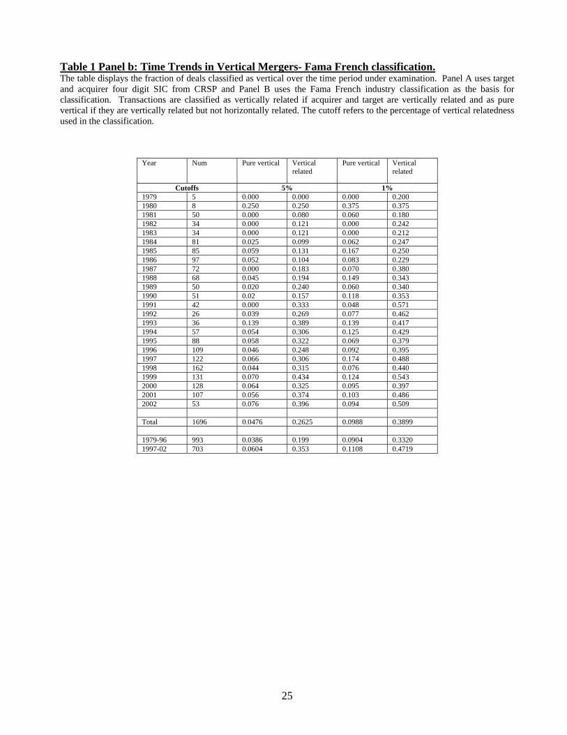
vertical deals. A similar trend is evident when we use Fama French industry classifications (See Panel
B). As Fama French industries are more broadly defined relative to four digit SIC, a larger fraction of
the vertically-related deals are also classified as horizontally-related. Consequently, the fraction of
deals classified as pure vertical is smaller relative to the four digit industry classification. Using a 1%
cutoff, only 9.88% of deals are classified as pure vertical when we use Fama French classification
compared to 21.58% with four digit SIC. This suggests that the use of different industry
classifications and cutoffs may have an impact on the categorization of mergers9.
We report most of our main results using four digit SIC classification, which is more precise, and a
1% cutoff. We also report the impact on these results as we move to stricter cutoffs and to Fama
French industry classification. Another feature of table 1, which is consistent with most other work
on mergers, is that it shows significant clusters over time in merger activities including merger waves
in the late 80’s and the late 90’s10. Also, it seems that vertical mergers were more prevalent in the late
80’s and late 90’s; however, it is difficult to point to a real time trend.
We consider acquirer and target wealth effects using standard event study methodology. We estimate
cumulative abnormal returns over the (−1, +1) day window using CRSP value-weighted index returns
with the parameters estimated over the 255 days estimation period that ends 46 days before the initial
merger announcement11. The total or aggregate return is the weighted return of the acquirer and
target, where weights are relative market capitalization ten days prior to the announcement.
9 Naturally, when we move from 1% to 5% and 10% cutoffs respectively, we lose quite a few observations. It does not seem that the average nature of the companies in question changes substantially, however. For example, for the1% sample, the average acquirer has assets of 6206 (in millions) whereas for the firms in the 5% cutoff, the average assets are 5986 (in millions). 10 See Moeller et al. (2005) and Andrade et al. (2001). 11 We also estimated a (-5, +5) window. Results are similar; however, given the many different classifications we already present, we do not include these tables. They are available upon request.
12
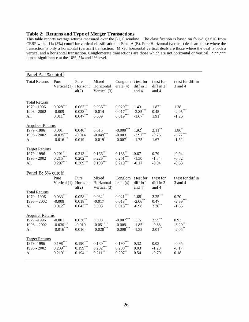
We find that pure vertical mergers are associated with positive total returns of 1.1% (See Table 2).
However, the average total return to vertical deals is significantly lower than the 4.7% earned by pure
horizontal mergers and is also lower than the 1.9% earned by conglomerate mergers. The better
performance of horizontal mergers is consistent with Fee and Thomas (2004), who cover a similar
time period, even though their definition of horizontal mergers is somewhat different than ours12.
The relative underperformance of vertical mergers with respect to conglomerate mergers, however, is
in contrast to Fan and Goyal (2006) who report significantly higher returns for vertical deals. When
we use Fama French Industries and a 5% cutoff for classifying vertical mergers, we find that although
the average returns to vertical mergers are still lower than returns for conglomerate mergers, this
difference is not significant (See Panel B). With other, different classifications, we continue to find
that vertical merger returns are lower than the returns of conglomerate mergers, although this
difference is not always statistically significant. To summarize, as far as we can tell, vertical mergers
are (at least weakly) worse than horizontal and conglomerate mergers. Mixed mergers seem to be
“bad” as well perhaps because they offer no clear rationale to investors.
In order to understand the difference between our results and Fan and Goyal (2006), we split our
sample into transactions before 1996 (Fan and Goyal sample period) and deals announced after 1996.
We find significant differences between the two sample periods. First, there appears to be a decline
in returns for all types of mergers after 1996. This is explored at length in Moeller et al. (2005).
However, there is a significantly greater decline in the performance of vertical mergers. The average
return to vertical deals was about 2.8% before 1996 and -0.9% (insignificant- that is, 0).after that. In
contrast, the return to horizontal deals is positive and significant (although declining) in both sub-
periods, and conglomerates show a lower positive but significant return in both sub-period. In other
words, whereas vertical deals had indeed performed better than conglomerate deals before 1996, as
documented by Fan and Goyal (2006), they performed worse after 1996. One explanation for the
lower returns to vertical deals after 1996 may be that they were not motivated by fundamental forces
in the industry that favored vertical integration13. We explore this further later.
Also, as discussed earlier, vertical deals were more frequent after 1996. Pure vertical mergers are
about 20% of all deals before 1996 and 25% after 1996 using four digit SIC and 1% cutoff. Thus, it
may be that after 1996 we moved lower on the diminishing returns curve.
12 For Fee and Thomas (2004) horizontal mergers mean a bidder and a target that have at least one industry segment in common. 13 Moeller et al.(2005) show that wealth destruction for acquirers in mergers accelerated from 1998 through 2001, which is consistent with our findings.
13
When we decompose total returns into target returns and acquirer returns, we find that, in line with
all prior literature starting from Bradley Desai and Kim (1988), including Andrade et al. (2001) and
more recently, Moeller et al. (2005), most of the value accrues to targets. Not surprisingly, target
returns are fairly similar across the different type of mergers and across the different time periods.
However, acquirer returns are negative and significant for vertical mergers in the later period. The
only other significance is for conglomerate, but the loss is much lower (less than 1% vs. 3% or more
for vertical acquirers). This sheds more light on our results and Fan and Goyal (2006).
Next we control for firm and deal characteristics. We control for the mode of payment by including a
dummy variable (Anystock) that takes the value one if stock is used for payment. As cash deals are
associated with higher returns in most other work, we expect the coefficient of Anystock to be
negative and significant. We control for acquirer size by including acquirer total assets in the year
prior to the announcement of the deal. We include the ratio of target size to acquire size
(TarSize_AcqSize) to control for relative size of the transaction. As small targets relative to the
acquirer are likely to have lower wealth effects, we expect the coefficient of relative size to be
positive. Naturally, we include a dummy for pure horizontal deals, pure vertical deals and mixed
horizontal vertical deals. Conglomerate is the default.
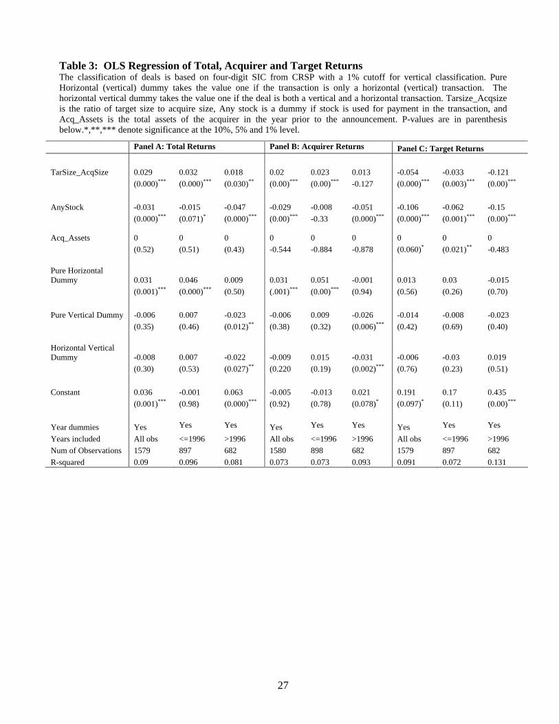
Table 3 contains OLS regressions. The findings are qualitatively similar to the univariate results
discussed above. Pure horizontal mergers feature significantly higher returns over the entire period,
in particular before 1996 (column 3). This is consistent with the findings of Shahrur (2005) and Fee
and Thomas (2004) who interpret the positive outcome of horizontal mergers as the result of
increases in efficiency and Gugler and Siebert (2007) who also find increases in efficiency following
horizontal mergers and joint ventures in the semiconductor industry. The coefficient of pure vertical
mergers is not significant for the whole sample, implying that pure vertical mergers are not different
from conglomerate mergers. However, for the period after 1996, pure vertical mergers are associated
with significantly lower total returns, after controlling for size, year dummies and the type of
transaction. These results are robust to different definitions of industry and different cutoffs for
vertical integration14. In line with the evidence in Table 2, we find that most of the returns accrue to
the target and further that target returns are not significantly different across merger types. It is the
significantly lower acquirer returns that drive the outcomes.
14 We do not report the results of using Fama French industry classifications and different cutoffs for brevity. The results are qualitatively similar and are available from the authors upon request. We note that mixed mergers tend to behave as vertical mergers, suggesting that at least for this specification, the vertical element may be dominant.
14
V. I/O DETERMINANTS OF VERTICAL MERGERS AND RETURNS
In this section, we test our hypotheses. It may be the case that, although vertical mergers at least
weakly destroy value, certain types of vertical mergers make economic sense.
5.1 Market Share and Industry Concentration
As discussed in Section 2, several theories proposed by Williamson (1971), Ordover, Saloner and
Salop (1990), and Tirole et. al (1990) Riordian (1998), Chen and Rirodan (2007), De Fontenay and
Gans, (2007) and many others, suggest that vertical integration can generate value in non-competitive
industries. These observations are summarized in hypothesis 1.While horizontal mergers can of
course thrive in such cases as well, there may be other rationales (such as economies of scale) which
can lead to successful horizontal integration.
In order to study the impact of acquirer and target industry market structures, we calculate target and
acquirer market shares. “Target market share” is defined as the sales of the target company divided
by industry total sales in the year prior to the announcement of the merger. “Industry” is defined by
four digit SIC classification and encompasses all firms with data in Compustat. Similarly, the acquirer
market share is the share of the acquirer in total industry sales. Since we expect most of the “action”
to be in the tails of the distribution, we create a dummy (High Share) that takes the value one when
both the acquirer and the target are in the top decile of all observations, in other words, are dominant
players in their respective industries. The top deciles include targets with market shares larger than
10% and acquirers with market shares in excess of 40% in their respective industries.
15
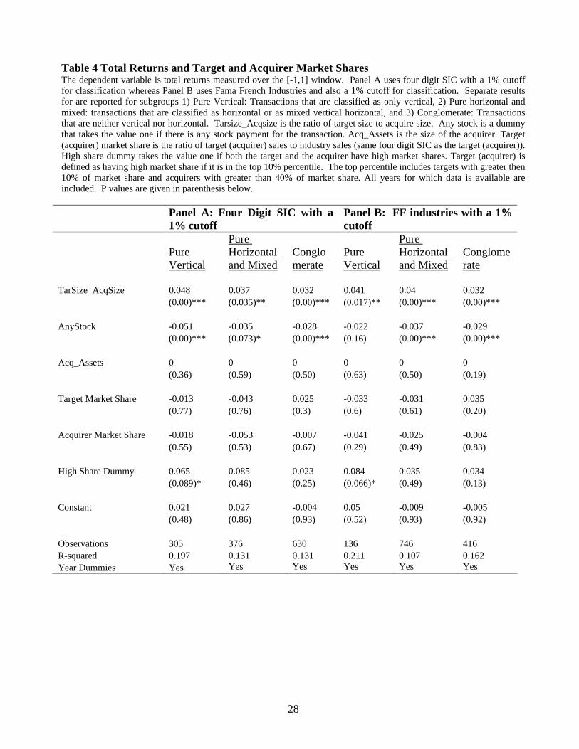
The results for this estimation are reported in Table 4. We estimate the model separately for each
type of merger, as the impact of market shares on total returns is likely to vary by merger type.15
Consistent with hypothesis 1, we find that when both the acquirer and the target are dominant players
in their respective industries, vertical mergers are associated with higher total returns. The high
market share is positive for all mergers, but it is most significant (at 9% and 7% respectively) for
vertical mergers.
This result that vertical mergers have higher returns when the target and acquirer are dominant firms
in the industry is fairly robust. When we use Fama French industry classifications (and a similar
cutoff of 1%) we continue to find that the High Share dummy is positive and significant (see Panel B,
Table 4). However, with a 5% cutoff for classifying vertical deals the high share dummy, although
still positive, loses significance. As discussed earlier, with these stricter criteria, there are fewer deals
that are classified as pure vertical and the small number of observations may account for the loss of
significance.
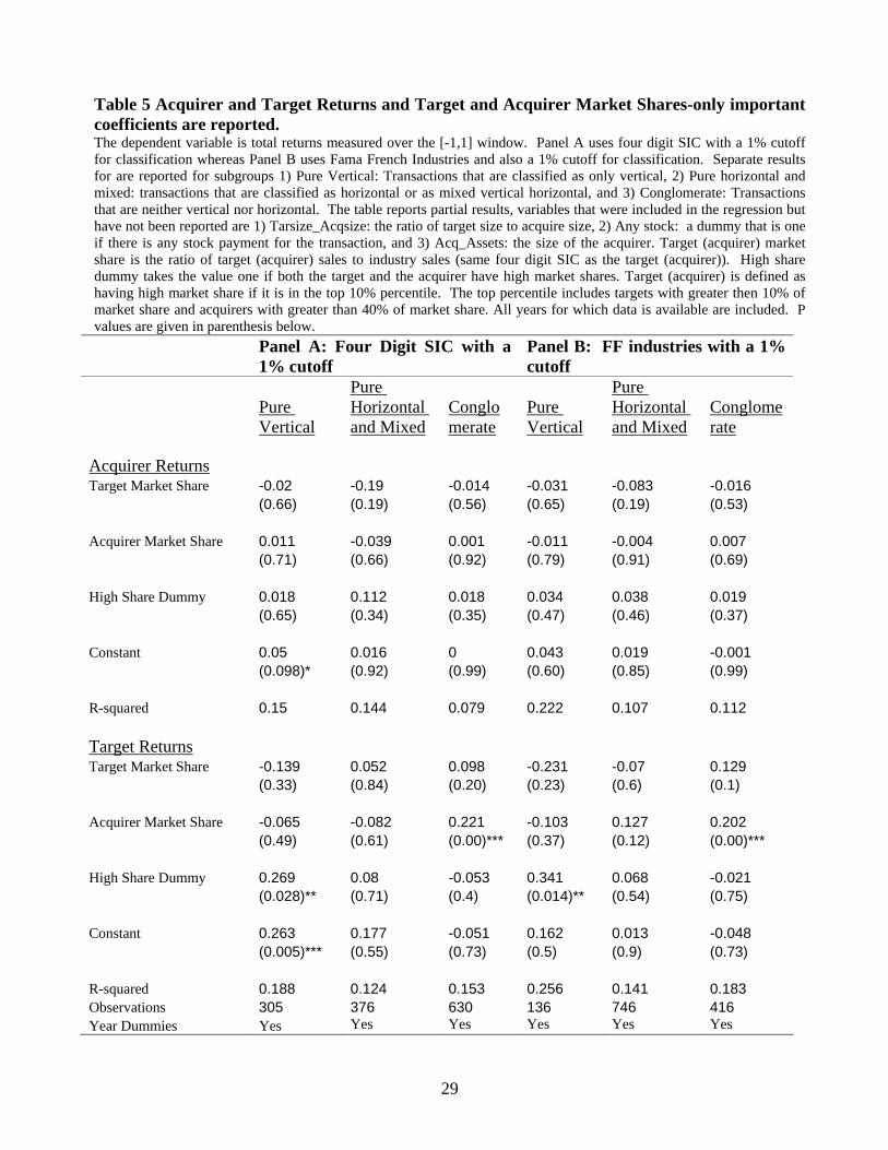
We also examine the distribution of total returns to targets and acquirers. 16 Consistent with the
previous discussion, the High Share dummy is not significant in explaining target and acquirer returns
except for vertical deals where it significantly increases target returns (See Table 5). This suggests that
the targets have higher bargaining power in situations where there are gains to be divided up in
vertical mergers. We notice that the market share variables are not significant for horizontal deals,
thus supporting the results of Fee and Thomas (2004) and Shahrur (2005)17.
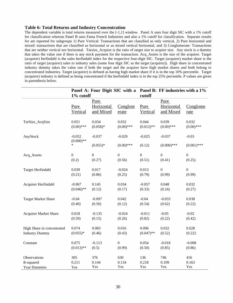
If the gains to vertical merger are based on the I/O theories discussed earlier, they should be more
noteworthy in concentrated industries. Dominant firms should have a greater ability to impose costs
on rivals in concentrated industries. In order to examine this idea, we also include target and acquirer
industry Herfindahl indices, calculated at the four digit SIC level. An industry is defined as a
concentrated industry if the Herfindahl index is the top quartile for all observations. In Table 6, we
include the Hefindahl dummy and an interactive dummy, which characterizes firms with large market
shares operating in concentrated industries. Vertical integration between dominant acquirers and
targets both operating in concentrated industries significantly increases total returns. CARs in these
cases are 7.5% higher than in other vertical mergers controlling for firm and deal characteristics. No 15 Alternatively, we could have run one regression including interaction terms of these market share variables with merger types. We choose not to report results in this way as it is cumbersome due to inclusion of so many interaction terms. We estimated this model and find that the results are similar. 16 Other factors, such as the number of competing bids, are likely to be important in determining the share of the target in the overall returns. However, these variables are not likely to be correlated with the type of merger. 17 Both papers suggest that anti-competitive motives do not drive vertical mergers.
16
such increase in returns can be observed for other types of mergers. As we can see in panel B, this
result is robust to using F-F industries to characterize the companies in our sample. We also observe a
negative and significant coefficient for the acquirer Herfindahl index, but only in one classification. We
are not sure how to interpret this coefficient. However, the overall picture is similar to the previous
table and consistent with work on horizontal mergers.
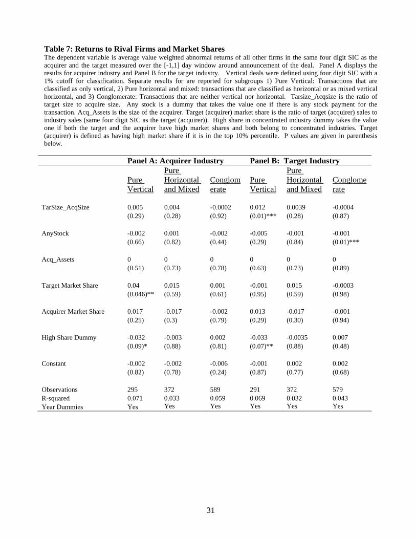
If the gain in vertical mergers, when the acquirer and target are large firms, is due to the increased ability
to impose costs on rival firms through rationing or price discrimination, then other firms in the industry
should experience negative returns on the announcement of the deal. In order to test this implication,
we calculate in table 7 abnormal returns for all firms in the acquirer’s industry, except the acquirer, over
the -1 to 1 day window surrounding the announcement of the transaction. We then calculate the market
value weighted average returns for all other firms in the industry. Similarly, we calculate the average
abnormal return to all other firms in the target firms industry. The average returns to competing firms
in both the acquirer and target industries are negative (and significant at 7% and 9% respectively
depending on the classification) when the acquirer and target have high market share in vertical deals.
There is no significant relation between market share of acquirer and target and returns to rival firms for
other types of mergers. This further supports the idea that gains in vertical mergers arise from an
increased ability to impose costs on rivals.
We should note that Fee and Thomas (2004) and Shahrur (2005) find that in horizontal mergers,
rivals’ returns are generally positive. Our findings and their results allow us to contrast the motives for
horizontal mergers (efficiency, according to their interpretation or as in Gugler and Siebert ,2007) with
the non-competitive flavor of vertical mergers in our sample. We also find that in 2.3% of all vertical
deals both the acquirer and the target have large shares. In comparison, in only 0.8% of the horizontal
mergers in our sample both the acquirer and target are large. This further supports the idea that
horizontal and vertical mergers are undertaken for different reasons. We also note that most of the
transactions that are classified as vertical deals between large acquirers and targets were announced
before 1996. If indeed a non-competitive market structure is required for a vertical mergers to succeed,
then the paucity of such mergers after 1996 may account for the worse outcomes (on average) for
vertical deals in the later part of our sample period.
In summary, our findings so far agree with the initial notion, going back to Williamson (1971) that
vertical integration will only be viable in a non-competitive environment. We can also offer support
for other models that follow the transaction costs hypotheses. Our results also agree with results in
17
the empirical I/O literature such as Lieberman (1991) which suggest that high concentrations increase
the probability of integration. It is interesting to see that both the acquirer and the target
concentrations matter, confirming the idea that indeed, non-competitive industries are the source of
gains in this type of mergers.
5.2 R&D Expenditures and Asset Specificity
In the presence of asset specificity, vertical integration may facilitate the alignment of incentives of
the two parties and ensure efficient investment. Consequently, Hypothesis 2 suggests that vertical
deals should be associated with higher total returns. As noted, we follow Caves and Bradburd (1988)
and use R&D expenditures normalized by sales to capture asset specificity. If both the acquirer and
the target engage in high levels of R&D, vertical integration may reduce the inefficiencies associated
with market exchanges of these assets. Empirically, we classify targets and acquirers as high R&D if
they are in the top deciles of R&D for the sample. This includes targets with 25% or more of sales
in R&D and acquirers with 40% or more of sales in R&D.
Consistent with hypothesis 2, we find that when target and acquirer are both high R&D firms, vertical
mergers are associated with higher total returns (see Table 8). Such deals are associated with 4%
higher returns relative to other vertical mergers. Further, there is no such gain to high R&D in other
type of mergers (the significance level is about 8%). The coefficient of acquirer R&D is negative and
significant for vertical deals. When Fama-French industry classifications are used, high R&D has
significantly higher returns although the coefficient for target R&D is negative and significant (See
Panel B). This suggests that as in the case of oligopolies, the “action” is in cases where both target
and acquirer are at the high end of the asset specificity range. Since R&D is a somewhat crude
measure of what we are trying to gauge, we see the impact when we focus on the more extreme cases.
We also note that most of the vertical mergers classified as being between acquirers and targets with
high R&D, were announced after 1996, suggesting that the motivation of vertical deals may have
shifted from exploiting competitive advantages to managing inefficiencies arising from asset
specificity over the sample period. The lower return to high R&D transactions relative to high-
market-share-transactions may explain at least partially the lower returns to vertical deals after 1996. It
also seems that acquirer and target R&D are significant for various types of mergers. The
interpretation may have to do with the ability to integrate specialized firms.
The result that vertical integration is associated with higher total returns when both targets and
acquirers are high R&D firms, holds when we use different industry classifications, namely, Fama
18
French or two-digit SIC. The result is less significant when we use stricter classification criteria, such
as a 5% cutoff to classify vertical mergers. As discussed above, the number of deals classified as pure
vertical drops with the stricter criteria and might account for the lack of significance18.
In summary, our findings thus far offer only some support for the “transaction costs” approach.
5.3 Information Asymmetry
To test hypothesis 3 i.e., the relationship between merger returns and available information about the
target and the acquirer, we gather data from the Institutional Brokers Estimate System (IBES) about
the number of analysts who provide earning estimates for the target and the acquirer in the year prior
to the merger announcement. The dummy Target Infodum takes a value of one if the target has no
analyst coverage. Similarly, the dummy Acquirer Infodum takes the value of one if the acquirer has
no analyst coverage. Finally, the dummy High Information Asymmetry takes the value one when
both the acquirer and the target have no analyst coverage.
There is no evidence that information asymmetry, as captured by analyst coverage, has any impact on
total returns in vertical deals as seen in Table 10. However, deals with a horizontal element seem to
be associated with higher returns in the presence of high information asymmetry. We can suggest
that when both the acquirer and the target have information problems with respect to the financial
markets, but operate in the same industry, it is likely that they are able to evaluate each other’s
prospects properly. It may not he possible for acquirers and targets that span different industries to
resolve their information problems via integration. In unreported results we find that the higher total
returns to horizontal mergers under high information asymmetry accrue mostly to acquirers. This is a
new result, as far as we know, and it reinforces the idea that horizontal mergers are more often done
for the right reasons.
5.4 Price Uncertainty
Finally, we examine the role of price uncertainty in making vertical integration valuable. We gather
data from the Bureau of Labor Statistics on the producer price index for the target and acquirer
industries. The Producer Price Index (PPI) program measures the average change over time in the
selling prices received by domestic producers for their output. As a measure of price uncertainty, we
compute the variance of the monthly PPI in the thirty-six months prior to the merger. In unreported
regressions, we observe that merger returns are unrelated to price uncertainty. The coefficient of our
18 These results are not reported in the paper for brevity but are available from the authors upon request.
19
uncertainty measures shifts between positive and negative for different classifications of vertical
integration and is never significant. Price uncertainty is also never significant in explaining returns in
other type of mergers. This does not support results of papers such as Lieberman (1991, for the
chemical industry). If indeed we could find a relationship, we could support models such as Carlton
(1977) which suggest that producing inputs internally (vertically integrating) can help a firm when
facing price uncertainty by allowing it to produce cheaply.
VI: Conclusions
In this paper we explore the market reactions to vertical mergers and correlate the returns with
predictions based on I/O theories.
Consistent with prior work, we find that horizontal mergers are on average, associated with
significantly higher returns and that these returns are time varying. Surprisingly, we find that vertical
mergers are very different. During our entire sample period, vertical merger returns have not been
significantly different from returns on conglomerate mergers. Similar to Fan and Goyal (2006), we
find that vertical mergers are associated with positive market reactions before 1996 but our work
shows that returns turn significantly negative later. We find support for the most fundamental insight
in the I/O literature, namely, that for vertical integration to work, we need firms that wield market
power in concentrated industries. This is not true for horizontal mergers. This latter result is
consistent with several recent studies which suggest that horizontal mergers are not motivated by
anti-competitive motives. We find less support for other suggested reasons for vertical integration. In
particular, we find only some support for the view that vertical mergers generate value when firms
invest in specialized assets making market exchanges difficult. There is little evidence to support the
view that information based contracting problems or price uncertainty, at least as captured in this
paper, generate a value maximizing rationale for vertical integration. However, informational
problems can increase returns to horizontal mergers.
If we were to formulate an overall conclusion which puts together the recent papers on horizontal
mergers, Fan and Goyal’s work, the recent study by Moeller et al. and our own work, we could
suggest that mergers undertaken for the right reasons can be beneficial, even to acquirers (although in
most cases targets still capture most of the gains).
Prior to 1996, many vertical mergers were undertaken for the “right” reasons, i.e. to take advantage of
a non-competitive market structure. Thus, the overall picture was positive. After 1996, the mix of
vertical mergers had changed, and thus market reactions to vertical mergers turned negative, even
relative to the general trend which featured many “bad” mergers. Horizontal mergers tend to be
undertaken for the right reasons more often, therefore they have always looked better. In fact, when
such mergers alleviate information issues, even acquirers can benefit.
20
REFERENCES:
Acemoglu, D. S. Johnson and T. Mitton, 2007, : “Determinants of Vertical Integration: Financial
Development and Contracting Costs” , working paper, MIT, May.
Anderson, Erin and David C. Schmittlein, 1984, Integration of the sales force: An empirical
Examination, Rand Journal of Economics 15, 385-395.
Andrade, G. M. Mitchell and E. Stafford, 2001, “New Evidence and Perspectives on Mergers” Journal
of Economic Perspectives, 15(2) Spring, pp. 102-120.
Arrow, Kenneth J., 1975, “Vertical integration and communication” Bell Journal of Economics, 6, pp. 171-
183.
Baker, G. R. Gibbons and K.J. Murphy, 2002,: “Rational Contracts and the Theory of the Firm”
Quarterly Journal of Economics Vol. 117, No. 1 (Feb), pp. 39-84
Berger, P. and E. Ofek ,1996, " Bustup Takeovers of Value Destroying Diversified Firms" Journal of
Finance, September, pp. 1175 - 1200.
Berger, P. and E. Ofek ,1995, “A Diversification Effect on Firm Value” Journal of Financial Economics,
37, pp. 39-65.
Bradley, M., A. Desai, and E. Kim "Synergistic Gains from Corporate Acquisitions and their Division
Between the Stockholders of Target and Acquiring Firms" Journal of Financial Economics, May 1988, 21,
3-40.
Campa, J.M and S. Kedia S,2002, “Explaining the Diversification Discount” Journal of Finance, August,
pp. 1731-1762.
Caves, R.E. and R.M. Bradburd, 1988, “ The Empirical Determinants of Vertical Integration” Journal of
Economic Behavior and Organization, Vol. 9 pp. 265-279
21
Chen, Y. and M. H. Riordan, 2007,: “Vertical Integration, Exclusive Dealing and Ex-Post
Cartelization”, Rand Journal of Economics vol. 38, #1, pp. 1-21
DeFontenay, C. and J. Gans, 2005, “Vertical Integration in the Presence of Upstream Competition”
Rand Journal of Economics vol. 36, Autumn 2005, pp. 544-572.
Eckbo, E. 1983, “Horizontal Mergers, Collusion and Stockholder Wealth” Journal of Financial Economics,
11, 241-273.
Eckbo, E. 1985, Mergers and the Market Power Doctrine: Evidence from the capital Markets” Journal
of Business, 58, 325-349.
Fan, J. and V. Goyal, 2006, “On the Patterns and Wealth Effects of Vertical Mergers” Journal of
Business, vol. 79 #21 pp. 877-902.
Fee, E. and S. Thomas, 2004.: “Sources of Gains in Horizontal Mergers: Evidence from Customer,
Supplier and Rival Firms” Journal of Financial Economics, 73, pp. 423-460.
Grossman, S. J. and O. Hart:, 1986, “ The Costs and Benefits of Ownership: a Theory of Vertical and
Lateral Integration” Journal of Political Economy, August, 94(4) pp. 691-719.
Gugler, K and R. Siebert, 2007, : “Market Power vs. Efficiency Effects of Mergers and Joint Research
Ventures : Evidence from the Semiconductor Industry” Review of Economics and Statistics, 89(4) pp. 645-
659.
Hughes, J.S. and J.L. Kao, 2001, “vertical Integration and Proprietary Information Transfers” Journal
of Economics and Management Strategy, vol. 10 #2 Summer, 277-299.
Hart, O. and J. Tirole , 1990, “Vertical Integration and Market foreclosure” 1990, Brookings Papers on
Economic Activity, Vol. 1990 pp. 205-286.
Joskow, P,1993, : “Asset specificity and the Structure of Vertical relationships: The empirical evidence”
in The nature of the Firm, in O.E. Williamson and S.E. Winter, Eds. Oxford University Press.
Kehoe, M.R. 1996, “Franchising Agency Problems and the Cost of Capital” Applied Economics, 28(11),
pp. 1485-93.
22
Klein, Benjamin, Robert G. Crawford and Armen A. Alchian, 1978, Vertical integration,
appropriable rents, and the competitive contracting process, Journal of Law and Economics
21, 297-336.
Klein, Benjamin, 1988 Klein, B. and K.M. Murphy,1997, “Vertical Integration as a Self Enforcing
Contractual Arrangement” American Economic Review, Vol 87. #2, May, pp. 415-420.
LaFontaine, F. and M. Slade, 2007,: “Vertical Integration and Firm Boundaries: the Evidence” Journal of
Economic Literature, September, Volume 135, # 3, pp.629-685.
Lieberman, M.A. (1991) “Determinants of Vertical Integration: An Empirical Test” The Journal of
Industrial Economics, 39(5) September, pp. 451-466.
McAfee, R. Preston and Marius Schwartz : “Opportunism in Multilateral Vertical Contracting:
Nondiscrimination, Exclusivity, and Uniformity” The American Economic Review, Vol. 84, No. 1 (Mar.,
1994), pp. 210-230
Masten, S.E., J. W. Meehan and E. A. Snyder, 1989, “Vertical integration in the U.S. auto industry : A
note on the influence of transaction specific assets” Journal of Economic Behavior & Organization, Volume
12, Issue 2, October, Pages 265-273
Moeller S. B. F.P. Schlingemann, and R.M. Stulz : “Wealth Destruction on a Massive Scale? A Study of
Acquiring Firm Returns in the Recent Merger Wave” Journal of Finance, 60(2), April, pp. 757-782.
Obanian, N.K. 1994, “Vertical Integration in the US Pulp and Paper Industry, 1900-1940” Review of
Economics and Statistics, 76 (1) pp. 202-207.
Ordover, J.A. G. Saloner and S.C. Salop (1990) “Equilibrium Vertical Foreclosure” American Economic
Review 80 (1) March 1990, pp. 127-142
Perry, M.K. (1978) “ Vertical Integration- the Monopsony case” American Economic Review, 68, 561-570.
Perry, M. K. (1989) “Vertical Integration: Determinants and Effects” in Schmallensee R. and R. Willig,
editors, Handbook of Industrial Organization, North Holland
23
Qiu, L. and W. Zhou, 2007, “ Merger Waves- a Model of Endogenous Mergers” Rand Journal of
Economics vol. 38, #1, pp. 214-226.
Rajan, Raghuram, Henri Servaes and Luigi Zingales, 2000, “The Cost of Diversity: The diversification
discount and inefficient investment” Journal of Finance, 55(1), 35-80.
Rhodes Kropf M. and S. Viswanathan, 2004, : “Market Valuation and Merger Waves” Journal of Finance,
December, p.2685-2718.
Riordan, M, 1998, “Anticompetitive Vertical Integration by a Dominant Firm” American Economic
Review, 88 (5), 1232-1248
Salinger, M. “Vertical Mergers and Market Foreclosure”, 1988, Quarterly Journal of Economics, Vol. 103,
#2, May, pp. 345-356.
Sappington, D. 2006, “On the Merits of Vertical Divestiture” Review of Industrial Organization, 29 (3), November, pp. 171-191. Schoar, Antoinette A ,2002, “The Effect of Corporate Firm Diversification on Firm Productivity”, Journal of Finance, December, 62 (6).
Shahrur, H. 2005, “Industry Structure and Horizontal Takeovers: Analysis of Wealth Effects on Rivals,
Suppliers and Corporate Customers” Journal of Financial Economics, 76, 61-98.
Uysal, V. Kedia, S. and V. Panchapagesan,2008, “Geography and acquirer returns” Journal of Financial
Intermediation, Volume 17, Issue 2, April, pp. 256-275.
Weiss, A.,1992, “The Role of Firm Specific Capital in Vertical Mergers” Journal of Law and Economics,
35(1), pp. 71-88.
Williamson, O, 1971, “The Vertical Integration of Production: Market Failure Considerations”
American Economic Review, 61, 112-123.
Williamson, O., 1983, “Credible Commitments Using Hostages to support Exchange”, American
Economic Review, 73(4): 519-40.
24
Table 1 Panel a : Time Trends in Vertical Mergers, 4 digit SIC classification. The table displays the fraction of deals classified as vertical over the time period under examination. Panel A uses target and acquirer four digit SIC from CRSP and Panel B uses the Fama French industry classification as the basis for classification. Transactions are classified as vertically related if acquirer and target are vertically related and as pure vertical if they are vertically related but not horizontally related. The cutoff refers to the percentage of vertical relatedness used in the table. . Year Num Pure vertical Vertical
related Pure vertical Vertical
related Pure vertical Vertical
related
Panel A: Industry is Four Digit SIC
Cutoffs 10% 5% 1% 1979 5 0.000 0.000 0.000 0.000 0.200 0.200 1980 8 0.250 0.250 0.250 0.250 0.375 0.375 1981 50 0.000 0.060 0.000 0.080 0.060 0.180 1982 34 0.029 0.059 0.059 0.147 0.059 0.265 1983 34 0.059 0.059 0.088 0.118 0.147 0.206 1984 81 0.049 0.049 0.062 0.099 0.162 0.247 1985 85 0.082 0.094 0.118 0.129 0.224 0.247 1986 97 0.022 0.041 0.062 0.103 0.124 0.227 1987 72 0.056 0.153 0.056 0.181 0.181 0.375 1988 68 0.074 0.103 0.118 0.191 0.250 0.338 1989 50 0.120 0.220 0.140 0.240 0.180 0.340 1990 51 0.098 0.137 0.118 0.157 0.255 0.353 1991 42 0.048 0.214 0.143 0.333 0.262 0.571 1992 26 0.039 0.039 0.231 0.269 0.385 0.462 1993 36 0.083 0.083 0.278 0.389 0.278 0.417 1994 57 0.035 0.105 0.123 0.298 0.211 0.421 1995 88 0.057 0.125 0.148 0.318 0.182 0.375 1996 109 0.018 0.055 0.119 0.248 0.229 0.395 1997 122 0.016 0.066 0.123 0.303 0.279 0.484 1998 162 0.043 0.074 0.161 0.309 0.259 0.432 1999 131 0.099 0.137 0.214 0.428 0.298 0.534 2000 128 0.031 0.109 0.109 0.320 0.148 0.391 2001 107 0.065 0.103 0.168 0.374 0.224 0.486 2002 53 0.057 0.094 0.208 0.396 0.264 0.509 Total 1696 0.0525 0.0973 0.1297 0.2606 0.2158 0.3868 1979-96 993 0.0534 0.0977 0.1088 0.1984 0.1954 0.3303 1997-02 703 0.0512 0.0967 0.1593 0.3485 0.2447 0.4666
25
Table 1 Panel b: Time Trends in Vertical Mergers- Fama French classification. The table displays the fraction of deals classified as vertical over the time period under examination. Panel A uses target and acquirer four digit SIC from CRSP and Panel B uses the Fama French industry classification as the basis for classification. Transactions are classified as vertically related if acquirer and target are vertically related and as pure vertical if they are vertically related but not horizontally related. The cutoff refers to the percentage of vertical relatedness used in the classification. Year Num Pure vertical Vertical
related Pure vertical Vertical
related
Cutoffs 5% 1% 1979 5 0.000 0.000 0.000 0.200 1980 8 0.250 0.250 0.375 0.375 1981 50 0.000 0.080 0.060 0.180 1982 34 0.000 0.121 0.000 0.242 1983 34 0.000 0.121 0.000 0.212 1984 81 0.025 0.099 0.062 0.247 1985 85 0.059 0.131 0.167 0.250 1986 97 0.052 0.104 0.083 0.229 1987 72 0.000 0.183 0.070 0.380 1988 68 0.045 0.194 0.149 0.343 1989 50 0.020 0.240 0.060 0.340 1990 51 0.02 0.157 0.118 0.353 1991 42 0.000 0.333 0.048 0.571 1992 26 0.039 0.269 0.077 0.462 1993 36 0.139 0.389 0.139 0.417 1994 57 0.054 0.306 0.125 0.429 1995 88 0.058 0.322 0.069 0.379 1996 109 0.046 0.248 0.092 0.395 1997 122 0.066 0.306 0.174 0.488 1998 162 0.044 0.315 0.076 0.440 1999 131 0.070 0.434 0.124 0.543 2000 128 0.064 0.325 0.095 0.397 2001 107 0.056 0.374 0.103 0.486 2002 53 0.076 0.396 0.094 0.509 Total 1696 0.0476 0.2625 0.0988 0.3899 1979-96 993 0.0386 0.199 0.0904 0.3320 1997-02 703 0.0604 0.353 0.1108 0.4719
26
Table 2: Returns and Type of Merger Transactions This table reports average returns measured over the [-1,1] window. The classification is based on four-digit SIC from CRSP with a 1% (5%) cutoff for vertical classification in Panel A (B). Pure Horizontal (vertical) deals are those where the transaction is only a horizontal (vertical) transaction. Mixed horizontal vertical deals are those where the deal is both a vertical and a horizontal transaction. Conglomerate transactions are those which are not horizontal or vertical. .*,**,*** denote significance at the 10%, 5% and 1% level. Panel A: 1% cutoff Total Returns Pure
Vertical (1) Pure Horizontal(2)
Mixed Horizontal Vertical (3)
Conglomerate (4)
t test for diff in 1 and 4
t test for diff in 2 and 4
t test for diff in 3 and 4
Total Returns 1979 –1996 0.028*** 0.063*** 0.036*** 0.020*** 1.43 1.87* 1.38 1996 - 2002 -0.009 0.023** -0.014 0.017*** -2.85*** 0.45 -2.95***
All 0.011** 0.047*** 0.009 0.019*** -1.67* 1.91* -1.26 Acquirer Returns 1979 -1996 0.001 0.040* 0.015 -0.009*** 1.92* 2.11** 1.86*
1996 - 2002 -0.035*** -0.014 -0.049*** -0.003 -2.97*** -0.76 -3.77***
All -0.016*** 0.019 -0.019** -0.007** -1.75* 1.67* -1.52 Target Returns 1979 -1996 0.201*** 0.213*** 0.166*** 0.188*** 0.67 0.79 -0.94 1996 - 2002 0.215*** 0.202*** 0.226*** 0.251*** -1.30 -1.34 -0.82 All 0.207*** 0.209*** 0.198*** 0.210*** -0.17 -0.04 -0.63 Panel B: 5% cutoff Pure
Vertical (1) Pure Horizontal(2)
Mixed Horizontal Vertical (3)
Conglomerate (4)
t test for diff in 1 and 4
t test for diff in 2 and 4
t test for diff in 3 and 4
Total Returns 1979 –1996 0.033*** 0.058*** 0.032* 0.021*** 1.68* 2.25*** 0.70 1996 – 2002 -0.008 0.018** -0.017 0.013** -2.06** 0.47 -2.59***
All 0.012** 0.043*** 0.003 0.018*** -0.98 2.26** -1.65 Acquirer Returns 1979 –1996 -0.001 0.036** 0.008 -0.007*** 1.15 2.55** 0.93 1996 – 2002 -0.030*** -0.019 -0.051*** -0.009 -1.85* -0.83 -3.29***
All -0.016*** 0.016 -0.028*** -0.008*** -1.33 2.01** -2.05**
Target Returns 1979 -1996 0.198*** 0.190*** 0.180*** 0.190*** 0.32 0.03 -0.35 1996 - 2002 0.239*** 0.199*** 0.232*** 0.238*** 0.03 -1.28 -0.17 All 0.219*** 0.194*** 0.211*** 0.207*** 0.54 -0.70 0.18
27
Table 3: OLS Regression of Total, Acquirer and Target Returns The classification of deals is based on four-digit SIC from CRSP with a 1% cutoff for vertical classification. Pure Horizontal (vertical) dummy takes the value one if the transaction is only a horizontal (vertical) transaction. The horizontal vertical dummy takes the value one if the deal is both a vertical and a horizontal transaction. Tarsize_Acqsize is the ratio of target size to acquire size, Any stock is a dummy if stock is used for payment in the transaction, and Acq_Assets is the total assets of the acquirer in the year prior to the announcement. P-values are in parenthesis below.*,**,*** denote significance at the 10%, 5% and 1% level.
Panel A: Total Returns Panel B: Acquirer Returns Panel C: Target Returns
TarSize_AcqSize 0.029 0.032 0.018 0.02 0.023 0.013 -0.054 -0.033 -0.121 (0.000)*** (0.000)*** (0.030)** (0.00)*** (0.00)*** -0.127 (0.000)*** (0.003)*** (0.00)*** AnyStock -0.031 -0.015 -0.047 -0.029 -0.008 -0.051 -0.106 -0.062 -0.15 (0.000)*** (0.071)* (0.000)*** (0.00)*** -0.33 (0.000)*** (0.000)*** (0.001)*** (0.00)*** Acq_Assets 0 0 0 0 0 0 0 0 0 (0.52) (0.51) (0.43) -0.544 -0.884 -0.878 (0.060)* (0.021)** -0.483 Pure Horizontal Dummy 0.031 0.046 0.009 0.031 0.051 -0.001 0.013 0.03 -0.015 (0.001)*** (0.000)*** (0.50) (.001)*** (0.00)*** (0.94) (0.56) (0.26) (0.70) Pure Vertical Dummy -0.006 0.007 -0.023 -0.006 0.009 -0.026 -0.014 -0.008 -0.023 (0.35) (0.46) (0.012)** (0.38) (0.32) (0.006)*** (0.42) (0.69) (0.40) Horizontal Vertical Dummy -0.008 0.007 -0.022 -0.009 0.015 -0.031 -0.006 -0.03 0.019 (0.30) (0.53) (0.027)** (0.220 (0.19) (0.002)*** (0.76) (0.23) (0.51) Constant 0.036 -0.001 0.063 -0.005 -0.013 0.021 0.191 0.17 0.435 (0.001)*** (0.98) (0.000)*** (0.92) (0.78) (0.078)* (0.097)* (0.11) (0.00)*** Year dummies Yes Yes Yes Yes Yes Yes Yes Yes Yes
Years included All obs <=1996 >1996 All obs <=1996 >1996 All obs <=1996 >1996 Num of Observations 1579 897 682 1580 898 682 1579 897 682 R-squared 0.09 0.096 0.081 0.073 0.073 0.093 0.091 0.072 0.131
28
Table 4 Total Returns and Target and Acquirer Market Shares The dependent variable is total returns measured over the [-1,1] window. Panel A uses four digit SIC with a 1% cutoff for classification whereas Panel B uses Fama French Industries and also a 1% cutoff for classification. Separate results for are reported for subgroups 1) Pure Vertical: Transactions that are classified as only vertical, 2) Pure horizontal and mixed: transactions that are classified as horizontal or as mixed vertical horizontal, and 3) Conglomerate: Transactions that are neither vertical nor horizontal. Tarsize_Acqsize is the ratio of target size to acquire size. Any stock is a dummy that takes the value one if there is any stock payment for the transaction. Acq_Assets is the size of the acquirer. Target (acquirer) market share is the ratio of target (acquirer) sales to industry sales (same four digit SIC as the target (acquirer)). High share dummy takes the value one if both the target and the acquirer have high market shares. Target (acquirer) is defined as having high market share if it is in the top 10% percentile. The top percentile includes targets with greater then 10% of market share and acquirers with greater than 40% of market share. All years for which data is available are included. P values are given in parenthesis below.
Panel A: Four Digit SIC with a 1% cutoff
Panel B: FF industries with a 1% cutoff
Pure Vertical
Pure Horizontal and Mixed
Conglomerate
Pure Vertical
Pure Horizontal and Mixed
Conglomerate
TarSize_AcqSize 0.048 0.037 0.032 0.041 0.04 0.032 (0.00)*** (0.035)** (0.00)*** (0.017)** (0.00)*** (0.00)*** AnyStock -0.051 -0.035 -0.028 -0.022 -0.037 -0.029 (0.00)*** (0.073)* (0.00)*** (0.16) (0.00)*** (0.00)*** Acq_Assets 0 0 0 0 0 0 (0.36) (0.59) (0.50) (0.63) (0.50) (0.19) Target Market Share -0.013 -0.043 0.025 -0.033 -0.031 0.035 (0.77) (0.76) (0.3) (0.6) (0.61) (0.20) Acquirer Market Share -0.018 -0.053 -0.007 -0.041 -0.025 -0.004 (0.55) (0.53) (0.67) (0.29) (0.49) (0.83) High Share Dummy 0.065 0.085 0.023 0.084 0.035 0.034 (0.089)* (0.46) (0.25) (0.066)* (0.49) (0.13) Constant 0.021 0.027 -0.004 0.05 -0.009 -0.005 (0.48) (0.86) (0.93) (0.52) (0.93) (0.92) Observations 305 376 630 136 746 416 R-squared 0.197 0.131 0.131 0.211 0.107 0.162 Year Dummies Yes Yes Yes Yes Yes Yes
29
Table 5 Acquirer and Target Returns and Target and Acquirer Market Shares-only important coefficients are reported. The dependent variable is total returns measured over the [-1,1] window. Panel A uses four digit SIC with a 1% cutoff for classification whereas Panel B uses Fama French Industries and also a 1% cutoff for classification. Separate results for are reported for subgroups 1) Pure Vertical: Transactions that are classified as only vertical, 2) Pure horizontal and mixed: transactions that are classified as horizontal or as mixed vertical horizontal, and 3) Conglomerate: Transactions that are neither vertical nor horizontal. The table reports partial results, variables that were included in the regression but have not been reported are 1) Tarsize_Acqsize: the ratio of target size to acquire size, 2) Any stock: a dummy that is one if there is any stock payment for the transaction, and 3) Acq_Assets: the size of the acquirer. Target (acquirer) market share is the ratio of target (acquirer) sales to industry sales (same four digit SIC as the target (acquirer)). High share dummy takes the value one if both the target and the acquirer have high market shares. Target (acquirer) is defined as having high market share if it is in the top 10% percentile. The top percentile includes targets with greater then 10% of market share and acquirers with greater than 40% of market share. All years for which data is available are included. P values are given in parenthesis below.
Panel A: Four Digit SIC with a 1% cutoff
Panel B: FF industries with a 1% cutoff
Pure Vertical
Pure Horizontal and Mixed
Conglomerate
Pure Vertical
Pure Horizontal and Mixed
Conglomerate
Acquirer Returns Target Market Share -0.02 -0.19 -0.014 -0.031 -0.083 -0.016 (0.66) (0.19) (0.56) (0.65) (0.19) (0.53) Acquirer Market Share 0.011 -0.039 0.001 -0.011 -0.004 0.007 (0.71) (0.66) (0.92) (0.79) (0.91) (0.69) High Share Dummy 0.018 0.112 0.018 0.034 0.038 0.019 (0.65) (0.34) (0.35) (0.47) (0.46) (0.37) Constant 0.05 0.016 0 0.043 0.019 -0.001 (0.098)* (0.92) (0.99) (0.60) (0.85) (0.99) R-squared 0.15 0.144 0.079 0.222 0.107 0.112 Target Returns Target Market Share -0.139 0.052 0.098 -0.231 -0.07 0.129 (0.33) (0.84) (0.20) (0.23) (0.6) (0.1) Acquirer Market Share -0.065 -0.082 0.221 -0.103 0.127 0.202 (0.49) (0.61) (0.00)*** (0.37) (0.12) (0.00)*** High Share Dummy 0.269 0.08 -0.053 0.341 0.068 -0.021 (0.028)** (0.71) (0.4) (0.014)** (0.54) (0.75) Constant 0.263 0.177 -0.051 0.162 0.013 -0.048 (0.005)*** (0.55) (0.73) (0.5) (0.9) (0.73) R-squared 0.188 0.124 0.153 0.256 0.141 0.183 Observations 305 376 630 136 746 416 Year Dummies Yes Yes Yes Yes Yes Yes
30
Table 6: Total Returns and Industry Concentration The dependent variable is total returns measured over the [-1,1] window. Panel A uses four digit SIC with a 1% cutoff for classification whereas Panel B uses Fama French Industries and also a 1% cutoff for classification. Separate results for are reported for subgroups 1) Pure Vertical: Transactions that are classified as only vertical, 2) Pure horizontal and mixed: transactions that are classified as horizontal or as mixed vertical horizontal, and 3) Conglomerate: Transactions that are neither vertical nor horizontal. Tarsize_Acqsize is the ratio of target size to acquire size. Any stock is a dummy that takes the value one if there is any stock payment for the transaction. Acq_Assets is the size of the acquirer. Target (acquirer) herfindahl is the sales herfindahl index for the respective four-digit SIC. Target (acquirer) market share is the ratio of target (acquirer) sales to industry sales (same four digit SIC as the target (acquirer)). High share in concentrated industry dummy takes the value one if both the target and the acquirer have high market shares and both belong to concentrated industries. Target (acquirer) is defined as having high market share if it is in the top 10% percentile. Target (acquirer) industry is defined as being concentrated if the herfindahl index is in the top 25% percentile. P values are given in parenthesis below.
Panel A: Four Digit SIC with a 1% cutoff
Panel B: FF industries with a 1% cutoff
Pure Vertical
Pure Horizontal and Mixed
Conglomerate
Pure Vertical
Pure Horizontal and Mixed
Conglomerate
TarSize_AcqSize 0.051 0.034 0.032 0.044 0.039 0.032 (0.00)*** (0.058)* (0.00)*** (0.012)** (0.00)*** (0.00)*** AnyStock -0.052 -0.037 -0.029 -0.025 -0.037 -0.03
(0.000)*** (0.055)* (0.00)*** (0.12) (0.000)*** (0.001)***
Acq_Assets 0 0 0 0 0 0 (0.2) (0.27) (0.56) (0.51) (0.41) (0.25) Target Herfindahl 0.039 0.017 -0.024 0.013 0 0 (0.21) (0.86) (0.25) (0.79) (0.99) (0.99) Acquirer Herfindahl -0.067 0.145 0.034 -0.057 0.048 0.032 (0.046)** (0.12) (0.17) (0.33) (0.24) (0.27) Target Market Share -0.04 -0.097 0.042 -0.04 -0.033 0.038 (0.40) (0.50) (0.12) (0.54) (0.62) (0.22) Acquirer Market Share 0.018 -0.135 -0.024 -0.011 -0.05 -0.02 (0.59) (0.15) (0.26) (0.82) (0.22) (0.42) High Share in concentrated 0.074 0.083 0.016 0.096 0.032 0.028 Industry Dummy (0.055)* (0.46) (0.43) (0.047)** (0.52) (0.222 Constant 0.075 -0.113 0 0.054 -0.018 -0.008 (0.013)** (0.5) (0.99) (0.50) (0.85) (0.86) Observations 305 376 630 136 746 416 R-squared 0.211 0.144 0.134 0.218 0.109 0.163 Year Dummies Yes Yes Yes Yes Yes Yes
31
Table 7: Returns to Rival Firms and Market Shares The dependent variable is average value weighted abnormal returns of all other firms in the same four digit SIC as the acquirer and the target measured over the [-1,1] day window around announcement of the deal. Panel A displays the results for acquirer industry and Panel B for the target industry. Vertical deals were defined using four digit SIC with a 1% cutoff for classification. Separate results for are reported for subgroups 1) Pure Vertical: Transactions that are classified as only vertical, 2) Pure horizontal and mixed: transactions that are classified as horizontal or as mixed vertical horizontal, and 3) Conglomerate: Transactions that are neither vertical nor horizontal. Tarsize_Acqsize is the ratio of target size to acquire size. Any stock is a dummy that takes the value one if there is any stock payment for the transaction. Acq_Assets is the size of the acquirer. Target (acquirer) market share is the ratio of target (acquirer) sales to industry sales (same four digit SIC as the target (acquirer)). High share in concentrated industry dummy takes the value one if both the target and the acquirer have high market shares and both belong to concentrated industries. Target (acquirer) is defined as having high market share if it is in the top 10% percentile. P values are given in parenthesis below.
Panel A: Acquirer Industry Panel B: Target Industry
Pure Vertical
Pure Horizontal and Mixed
Conglomerate
Pure Vertical
Pure Horizontal and Mixed
Conglomerate
TarSize_AcqSize 0.005 0.004 -0.0002 0.012 0.0039 -0.0004 (0.29) (0.28) (0.92) (0.01)*** (0.28) (0.87) AnyStock -0.002 0.001 -0.002 -0.005 -0.001 -0.001 (0.66) (0.82) (0.44) (0.29) (0.84) (0.01)*** Acq_Assets 0 0 0 0 0 0 (0.51) (0.73) (0.78) (0.63) (0.73) (0.89) Target Market Share 0.04 0.015 0.001 -0.001 0.015 -0.0003 (0.046)** (0.59) (0.61) (0.95) (0.59) (0.98) Acquirer Market Share 0.017 -0.017 -0.002 0.013 -0.017 -0.001 (0.25) (0.3) (0.79) (0.29) (0.30) (0.94) High Share Dummy -0.032 -0.003 0.002 -0.033 -0.0035 0.007 (0.09)* (0.88) (0.81) (0.07)** (0.88) (0.48) Constant -0.002 -0.002 -0.006 -0.001 0.002 0.002 (0.82) (0.78) (0.24) (0.87) (0.77) (0.68) Observations 295 372 589 291 372 579 R-squared 0.071 0.033 0.059 0.069 0.032 0.043 Year Dummies Yes Yes Yes Yes Yes Yes
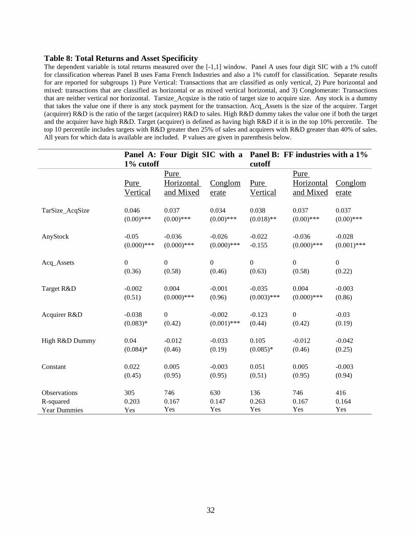
32
Table 8: Total Returns and Asset Specificity The dependent variable is total returns measured over the [-1,1] window. Panel A uses four digit SIC with a 1% cutoff for classification whereas Panel B uses Fama French Industries and also a 1% cutoff for classification. Separate results for are reported for subgroups 1) Pure Vertical: Transactions that are classified as only vertical, 2) Pure horizontal and mixed: transactions that are classified as horizontal or as mixed vertical horizontal, and 3) Conglomerate: Transactions that are neither vertical nor horizontal. Tarsize_Acqsize is the ratio of target size to acquire size. Any stock is a dummy that takes the value one if there is any stock payment for the transaction. Acq_Assets is the size of the acquirer. Target (acquirer) R&D is the ratio of the target (acquirer) R&D to sales. High R&D dummy takes the value one if both the target and the acquirer have high R&D. Target (acquirer) is defined as having high R&D if it is in the top 10% percentile. The top 10 percentile includes targets with R&D greater then 25% of sales and acquirers with R&D greater than 40% of sales. All years for which data is available are included. P values are given in parenthesis below.
Panel A: Four Digit SIC with a 1% cutoff
Panel B: FF industries with a 1% cutoff
Pure Vertical
Pure Horizontal and Mixed
Conglomerate
Pure Vertical
Pure Horizontal and Mixed
Conglomerate
TarSize_AcqSize 0.046 0.037 0.034 0.038 0.037 0.037 (0.00)*** (0.00)*** (0.00)*** (0.018)** (0.00)*** (0.00)*** AnyStock -0.05 -0.036 -0.026 -0.022 -0.036 -0.028 (0.000)*** (0.000)*** (0.000)*** -0.155 (0.000)*** (0.001)*** Acq_Assets 0 0 0 0 0 0 (0.36) (0.58) (0.46) (0.63) (0.58) (0.22) Target R&D -0.002 0.004 -0.001 -0.035 0.004 -0.003 (0.51) (0.000)*** (0.96) (0.003)*** (0.000)*** (0.86) Acquirer R&D -0.038 0 -0.002 -0.123 0 -0.03 (0.083)* (0.42) (0.001)*** (0.44) (0.42) (0.19) High R&D Dummy 0.04 -0.012 -0.033 0.105 -0.012 -0.042 (0.084)* (0.46) (0.19) (0.085)* (0.46) (0.25) Constant 0.022 0.005 -0.003 0.051 0.005 -0.003 (0.45) (0.95) (0.95) (0.51) (0.95) (0.94) Observations 305 746 630 136 746 416 R-squared 0.203 0.167 0.147 0.263 0.167 0.164 Year Dummies Yes Yes Yes Yes Yes Yes
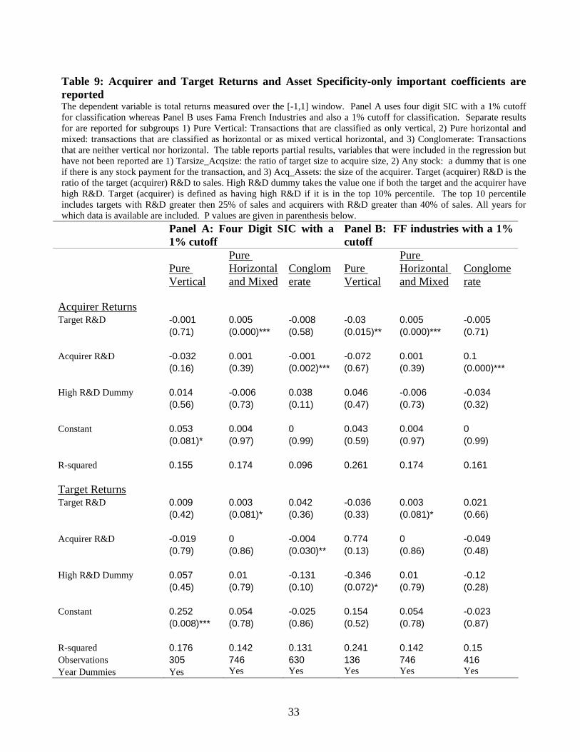
33
Table 9: Acquirer and Target Returns and Asset Specificity-only important coefficients are reported The dependent variable is total returns measured over the [-1,1] window. Panel A uses four digit SIC with a 1% cutoff for classification whereas Panel B uses Fama French Industries and also a 1% cutoff for classification. Separate results for are reported for subgroups 1) Pure Vertical: Transactions that are classified as only vertical, 2) Pure horizontal and mixed: transactions that are classified as horizontal or as mixed vertical horizontal, and 3) Conglomerate: Transactions that are neither vertical nor horizontal. The table reports partial results, variables that were included in the regression but have not been reported are 1) Tarsize_Acqsize: the ratio of target size to acquire size, 2) Any stock: a dummy that is one if there is any stock payment for the transaction, and 3) Acq_Assets: the size of the acquirer. Target (acquirer) R&D is the ratio of the target (acquirer) R&D to sales. High R&D dummy takes the value one if both the target and the acquirer have high R&D. Target (acquirer) is defined as having high R&D if it is in the top 10% percentile. The top 10 percentile includes targets with R&D greater then 25% of sales and acquirers with R&D greater than 40% of sales. All years for which data is available are included. P values are given in parenthesis below.
Panel A: Four Digit SIC with a 1% cutoff
Panel B: FF industries with a 1% cutoff
Pure Vertical
Pure Horizontal and Mixed
Conglomerate
Pure Vertical
Pure Horizontal and Mixed
Conglomerate
Acquirer Returns Target R&D -0.001 0.005 -0.008 -0.03 0.005 -0.005 (0.71) (0.000)*** (0.58) (0.015)** (0.000)*** (0.71) Acquirer R&D -0.032 0.001 -0.001 -0.072 0.001 0.1 (0.16) (0.39) (0.002)*** (0.67) (0.39) (0.000)*** High R&D Dummy 0.014 -0.006 0.038 0.046 -0.006 -0.034 (0.56) (0.73) (0.11) (0.47) (0.73) (0.32) Constant 0.053 0.004 0 0.043 0.004 0 (0.081)* (0.97) (0.99) (0.59) (0.97) (0.99) R-squared 0.155 0.174 0.096 0.261 0.174 0.161 Target Returns Target R&D 0.009 0.003 0.042 -0.036 0.003 0.021 (0.42) (0.081)* (0.36) (0.33) (0.081)* (0.66) Acquirer R&D -0.019 0 -0.004 0.774 0 -0.049 (0.79) (0.86) (0.030)** (0.13) (0.86) (0.48) High R&D Dummy 0.057 0.01 -0.131 -0.346 0.01 -0.12 (0.45) (0.79) (0.10) (0.072)* (0.79) (0.28) Constant 0.252 0.054 -0.025 0.154 0.054 -0.023 (0.008)*** (0.78) (0.86) (0.52) (0.78) (0.87) R-squared 0.176 0.142 0.131 0.241 0.142 0.15 Observations 305 746 630 136 746 416 Year Dummies Yes Yes Yes Yes Yes Yes
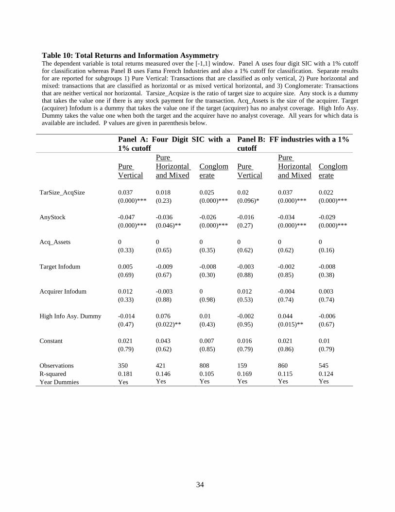
34
Table 10: Total Returns and Information Asymmetry The dependent variable is total returns measured over the [-1,1] window. Panel A uses four digit SIC with a 1% cutoff for classification whereas Panel B uses Fama French Industries and also a 1% cutoff for classification. Separate results for are reported for subgroups 1) Pure Vertical: Transactions that are classified as only vertical, 2) Pure horizontal and mixed: transactions that are classified as horizontal or as mixed vertical horizontal, and 3) Conglomerate: Transactions that are neither vertical nor horizontal. Tarsize_Acqsize is the ratio of target size to acquire size. Any stock is a dummy that takes the value one if there is any stock payment for the transaction. Acq_Assets is the size of the acquirer. Target (acquirer) Infodum is a dummy that takes the value one if the target (acquirer) has no analyst coverage. High Info Asy. Dummy takes the value one when both the target and the acquirer have no analyst coverage. All years for which data is available are included. P values are given in parenthesis below.
Panel A: Four Digit SIC with a 1% cutoff
Panel B: FF industries with a 1% cutoff
Pure Vertical
Pure Horizontal and Mixed
Conglomerate
Pure Vertical
Pure Horizontal and Mixed
Conglomerate
TarSize_AcqSize 0.037 0.018 0.025 0.02 0.037 0.022 (0.000)*** (0.23) (0.000)*** (0.096)* (0.000)*** (0.000)*** AnyStock -0.047 -0.036 -0.026 -0.016 -0.034 -0.029 (0.000)*** (0.046)** (0.000)*** (0.27) (0.000)*** (0.000)*** Acq_Assets 0 0 0 0 0 0 (0.33) (0.65) (0.35) (0.62) (0.62) (0.16) Target Infodum 0.005 -0.009 -0.008 -0.003 -0.002 -0.008 (0.69) (0.67) (0.30) (0.88) (0.85) (0.38) Acquirer Infodum 0.012 -0.003 0 0.012 -0.004 0.003 (0.33) (0.88) (0.98) (0.53) (0.74) (0.74) High Info Asy. Dummy -0.014 0.076 0.01 -0.002 0.044 -0.006 (0.47) (0.022)** (0.43) (0.95) (0.015)** (0.67) Constant 0.021 0.043 0.007 0.016 0.021 0.01 (0.79) (0.62) (0.85) (0.79) (0.86) (0.79) Observations 350 421 808 159 860 545 R-squared 0.181 0.146 0.105 0.169 0.115 0.124 Year Dummies Yes Yes Yes Yes Yes Yes