Vertical shear instability in accretion disc models with ... · Astronomy & Astrophysics manuscript no. vsi-paper c ESO 2014 October 1, 2014 Vertical shear instability in accretion

Astronomy & Astrophysics manuscript no. vsi-paper c©ESO 2018November 5, 2018

Vertical shear instability in accretion disc models with radiationtransport

Moritz H. R. Stoll and Wilhelm Kley

Institut für Astronomie und Astrophysik, Universität Tübingen, Auf der Morgenstelle 10, D-72076 Tübingen, Germanye-mail: [email protected],[email protected]

Received 2014-05-05; accepted 2014-09-25

ABSTRACT

Context. The origin of turbulence in accretion discs is still not fully understood. While the magneto-rotational instability is consideredto operate in sufficiently ionized discs, its role in the poorly ionized protoplanetary disc is questionable. Recently, the vertical shearinstability (VSI) has been suggested as a possible alternative.Aims. Our goal is to study the characteristics of this instability and the efficiency of angular momentum transport, in extended discs,under the influence of radiative transport and irradiation from the central star.Methods. We use multi-dimensional hydrodynamic simulations to model a larger section of an accretion disc. First we study inviscidand weakly viscous discs using a fixed radial temperature profile in two and three spatial dimensions. The simulations are thenextended to include radiative transport and irradiation from the central star.Results. In agreement with previous studies we find for the isothermal disc a sustained unstable state with a weak positive angularmomentum transport of the order of α ≈ 10−4. Under the inclusion of radiative transport the disc cools off and the turbulenceterminates. For discs irradiated from the central star we find again a persistent instability with a similar α value as for the isothermalcase.Conclusions. We find that the VSI can indeed generate sustained turbulence in discs albeit at a relatively low level with α about fewtimes 10−4.

Key words. instability – hydrodynamics – accretion discs – radiative transfer

1. Introduction

The origin of the angular momentum transport in accretion discsis still not fully understood. Observationally it is well confirmedthat the molecular viscosity is by many orders of magnitudetoo small to explain the effective mass and angular momentumtransport in discs (Pringle 1981). This can be inferred for ex-ample from time variations of the disc luminosity in close bi-nary systems, or by correlating the infrared-excess caused bydiscs around young stars with the age of the system. As a con-sequence it is assumed that discs are driven by some kind ofturbulent transport whose cause is still not known. Despite itsunknown origin the efficiency of the turbulence is usually pa-rameterized in terms of the dimensionless parameter, α, as intro-duced by Shakura & Sunyaev (1973). Observationally, values ofa few times 10−3 as in protostellar discs to 10−1 for discs in closebinary stars are suggested. For sufficiently well ionized discs themagnetorotational instability (MRI) is certainly the most promis-ing candidate to provide the transport (Balbus 2003). While thismay be true for the hot discs in close binary systems or in ac-tive galactic nuclei, there is the important class of protostellardiscs where at least the thermal ionisation levels are too low toprovide a sufficient number of charged particles that can supportthe MRI (Armitage 2011). In such discs the turbulence plays animportant role in several aspects. Not only does it determine thelifetime of an accretion disc, but it also influences where and howplanets can form and evolve in the disc. A variety of sourcessuch as stellar X-rays, cosmic rays or collisions with beta par-

ticles from radioactive nuclei have been invoked to provide therequired ionization levels but recent studies indicate the presenceof an extended ’dead zone’ where, due to the lack of ionization,no magnetically driven instability may operate. Additionally, re-cent studies on the origins of turbulence in protostellar discs thatinclude non-ideal magnetohydrodynamical (MHD) effects suchas ambipolar diffusion or the Hall effect, indicate that the MRImay even be suppressed strongly in these discs, see the reviewby Turner et al. (2014) and references therein.

As a consequence alternative mechanisms to provide tur-bulence are actively discussed. Typical examples for non-magnetized discs are the convective instability (Ruden et al.1988), the gravitational instability (Lin & Pringle 1987), or thebaroclinic instability (Klahr & Bodenheimer 2003), for furtherreferences see Nelson et al. (2013). While any of these mayoperate under special conditions in the disc, e.g. suitable ra-dial entropy gradients or a sufficiently high disc mass, noneseems to have general applicability. Searching for alternativesthe vertical shear instability (VSI) has attracted recent interest.Here, the instability is caused by a vertical gradient of the angu-lar velocity, Ω, in the disc. Through linear analysis it has beenshown that for a sufficiently strong vertical shear there are al-ways modes that can overcome the stabilizing angular momen-tum gradient (Rayleigh-criterion) and generate instability (Urpin& Brandenburg 1998; Urpin 2003). This instability is related tothe Goldreich-Schubert-Fricke instability that can occur in dif-ferentially rotating stars (Goldreich & Schubert 1967; Fricke1968).

Article number, page 1 of 12

arX

iv:1

409.

8429

v1 [

astr

o-ph

.EP]

30

Sep

2014

A&A proofs: manuscript no. vsi-paper

Concerning its effectiveness with respect to angular momen-tum transport numerical simulations were performed by Arlt &Urpin (2004) and Nelson et al. (2013). The first authors anal-ysed the instability for globally isothermal discs and found thatthe instability in this case could only be triggered by applying fi-nite initial perturbation because the equilibrium state of the disc(being strictly isothermal) did not contain a shear in Ω. The max-imum values of α obtained by Arlt & Urpin (2004) were around6 · 10−6 but the turbulence was decaying in the long run. Nelsonet al. (2013) extended these simulations and performed high res-olution simulations of the VSI for so called locally isothermaldiscs that contain a radial temperature gradient but are verticallyisothermal. Under these conditions the equilibrium state has avertical gradient in the shear and indeed an instability sets in.As shown by Nelson et al. (2013) the instability has two dis-tinct growth phases, it starts from the surface layers of the discwhere the shear is strongest and then protrudes towards the mid-plane. In the final state the vertical motions in the disc are an-tisymmetric with respect to the discs’s midplane, such that thegas elements cross the midplane, a feature found for the verti-cal convective motions in discs as well (Kley et al. 1993). Forthe efficiency of the VSI induced turbulence Nelson et al. (2013)found a weak angular momentum transport with α = 6 · 10−4.They also showed that under the presence of a small viscosityor thermal relaxation the instability is weaker and can easily bequenched.

It is not clear what influence radiation transport will have onthis instability. Without external heat sources one might expectthat, because of radiative cooling and the dependence of the in-stability on temperature, the instability will die out. Here, weevaluate the evolution of the instability for a radiative discs andan ideal equation of state. Additionally, we extend the radial do-main and include irradiation from the central star. We performtwo-dimensional and three-dimensional hydrodynamical simu-lations including radiative transport.

This paper is organized as follows. In Section 2, we presentthe physical setup of our disc models and in Section 3 the numer-ical approach. The isothermal results are presented in Section 4,followed by the radiative cases in Section 5. Stellar irradiation isconsidered in Section 6 and in Section 7 we conclude.

2. Physical setup

In order to study the VSI of the disc in the presence of radiativetransport we construct numerical models solving the hydrody-namical equations for a section of the accretion disc in two andthree spatial dimensions.

2.1. Equations

The basis our studies are the Euler equations (1 - 3) describingthe motion of an ideal gas. These are coupled to radiation trans-port (4) for which we use the two temperature approximationapplying flux-limited diffusion. The equations then read

∂ρ

∂t+ ∇(ρu) = 0 (1)

∂

∂tρu + ∇(ρuu) + ∇p = ρaext (2)

∂

∂te + ∇[(e + p)u] = ρuaext − κPρc(aRT 4 − E) (3)

∂

∂tE + ∇F = κPρc

(aRT 4 − E

). (4)

Here ρ is the density, u the velocity, e the total energy density(kinetic and thermal) of the gas. p denotes the gas pressure, andthe acceleration due to external forces, such as the gravitationalforce exerted by the central star is given by aext. E and F arethe energy density and the flux of the radiation. The last termson the r.h.s. of eqs. (3) and (4) refer to the coupling of gas andradiation, i.e. the heating/cooling terms. Here, c stands for thespeed of light, aR is the radiation constant, and κP the Plank meanopacity.

We close the equations with the ideal gas equation of state

p = (γ − 1)eth , (5)

where eth = e − 1/2ρu2 is the thermal energy density. The tem-perature of the gas is then calculated from

p = ρkBTµmH

, (6)

where µ is the mean molecular weight, kB the Boltzmann con-stant and mH the mass of the hydrogen atom. In our simulationswith radiation transport we use γ = 1.4 and µ = 2.35. To com-pare to previous studies we performed additional isothermal sim-ulations where we use γ = 1.001 and additionally reset to theoriginal temperature profile in every step. This procedure corre-sponds to an isothermal simulation but allows for an arbitrarytemperature profile. It also allows to use the feature of slowly re-laxing to a given original temperature such as used for examplein Nelson et al. (2013). Note that without resetting the tempera-ture the gas remains adiabatic, and the perturbation will die outfor our setup.

The radiation flux in the flux-limited diffusion (FLD) ap-proximation (Levermore & Pomraning 1981) is given by

F = −λcκRρ∇E , (7)

where κR is the Rosseland mean opacity and λ is the flux-limiter,for which we use the description of Minerbo (1978). For theRosseland mean opacity we apply the model of Bell & Lin(1994). For simplicity we use in this initial study the same valuefor the Plank mean opacity, see also Bitsch et al. (2013).

In some of our studies we add viscosity and stellar irradiationto the momentum and energy equations. This will be pointed outbelow in the appropriate sections.

2.2. Disc model

To be able to study the onset of the instability we start with a ref-erence model in equilibrium. For this purpose, we follow Nelsonet al. (2013) and use a locally isothermal disc in force equilib-rium, where for the midplane density we assume a power lawbehaviour

ρ(R,Z = 0) = ρ0

(RR0

)p

, (8)

and the temperature is constant on cylinders

T (R,Z) = T0

(RR0

)q

. (9)

To specify the equilibrium state we have used a cylindrical co-ordinate system (R,Z, φ). However, our simulations will be per-formed in spherical polar coordinates (r, θ, φ) because they arebetter adapted to the geometry of an accretion disc. In eqs. (8)


Moritz H. R. Stoll and Wilhelm Kley: Vertical shear instability in accretion disc models with radiation transport

and (9), ρ0 and T0 are suitably chosen constants that determinethe total mass content in the disc and its temperature. The ex-ponents p and q give the radial steepness of the profiles, andtypically we choose p = −3/2 and q = −1. Assuming that inthe initial state there are no motions in the meridional plane andthe flow is purely toroidal, force balance in the radial and verti-cal directions then leads to the equilibrium density and angularvelocity profiles that we use for the initial setup (Nelson et al.2013)

ρ(R,Z) = ρ0

(RR0

)p

exp[GMc2

s

(1

√R2 + Z2

−1R

)], (10)

and

Ω(R,Z) = ΩK

[(p + q)

(HR

)2

+ (1 + q) −qR

√R2 + Z2

] 12

. (11)

Here, cs =√

p/ρ denotes the isothermal sound speed, ΩK =√GM/R3 the Keplerian angular velocity, and H = cs/ΩK is the

local pressure scale height of the accretion disc. We note that theZ dependence of Ω in the equilibrium state is the origin of theVSI, because the vertical shear provides the opportunity for fluidperturbations with a wavenumber ratio kR/kZ above a thresholdto tap into a negative gradient in the angular momentum as theperturbed fluid elements move away from the rotation axis (Nel-son et al. 2013). The angular velocity given by eq. (11) is alsoused to calculate the Reynolds stress tensor, for details see be-low.

2.3. Stability

Nelson et al. (2013) repeated the original analysis in Goldreich &Schubert (1967) for a locally isothermal and compressive gas foran accretion disc using the local shearing sheet approximation ata reference radius r0. They derived the same stability criterionas Urpin (2003) and obtained the following growth rate of theinstability

σ2 =−κ2

0(c20k2

Z + N20 ) + 2Ω0c2

0kRkZ∂V∂z

c20(k2

Z + k2R) + κ2

0 + N20

, (12)

where κ0 is the epicyclic frequency, c0 the sound speed, and N0is the Brunt-Vaisaila frequency at the radius r0. V denotes themean deviation from of the Keplerian azimuthal velocity profile,and kR, kZ are the radial and vertical wavenumbers of the pertur-bations in the local coordinates.

For negligible N0, small H0/R0, and kZ/kR ∼ O(qH0/R0), asseen in their numerical simulations, Nelson et al. (2013) find

σ ∼ qΩHR, (13)

which implies that the growth rate per local orbit to first orderdepends on the temperature gradient as given by q and on theabsolute temperature, due to H/R. We will compare our numeri-cal results with these estimates.

3. Numerical Model

To study the VSI in the presence of radiative transport we per-form numerical simulations of a section of an accretion disc intwo and three spatial dimensions using spherical polar coordi-nates (r, θ, φ), and a grid which is logarithmic in radial direc-tion, keeping the cells squared. We solve eqs. (1) to (4) with a

grid based method, where we use the PLUTO code from Mignoneet al. (2007) that utilizes a second-order Godunov scheme, to-gether with our radiation transport (Kolb et al. 2013) in the FLDapproximation, see eq. (7).

The simulations span a region in radius from r = 2 − 10AU,this is the range where the dead zone can be expected (Armitage2011; Flaig et al. 2012). Here, we use a larger radial domain asNelson et al. (2013) because we intend to study the global prop-erties of the instability over a wider range of distances. Addition-ally, this larger range is useful, because we need some additionalspace (typically ≈ 1AU) to damp possible large scale vorticesin the meridional plane that show up at the inner radial bound-ary of the domain (see below). The origin of these vortices ispossibly that the instability moves material along cylindricallyshaped shells, a motion that is not adapted to the used sphericalcoordinates, such that the midplane is cut out at the inner bound-ary. Vortices can also arise if the viscosity changes apruptly, asituation mimicking a boundary. Additionally, in some cases thewavelengths are large, such that the coupling between differentmodes cannot be captured in a small domain. Also we use a widerange because with radiation transport the growth rates are ex-pected to depend on the opacity, which is a function of ρ and Tand thus of the radius. In the meridional direction (θ) we go up to±5 scale heights above and below the equator in the isothermalcase, and we use the same extension for the radiative simulation,where it corresponds to more scale heights. For the 3D simula-tions we used in the azimuthal direction (φ) a quarter circle, from0 to π/2.

We use reflective boundaries in the radial direction. In themeridional direction we use outflow conditions for the flow outof the domain and reflective conditions otherwise. For the radi-ation transport solver we set the temperature of the meridionalboundary to 10K, which allows the radiation to escape freely.We use damping of the velocity near the inner radial boundarywithin 2 − 3AU to prevent the creation of strong vortices arisingthrough the interaction with the reflecting boundary, which candestroy the simulation. This is done by adding a small viscosityof ν = 2 · 10−7 with a linear decrease to zero from 2AU to 3AU(similar to the damping used in de Val-Borro et al. (2006)).

We assume that the disc orbits a solar mass star and we applya density of ρ0 = 10−10g/cm3 at 1AU. Due to the surface densitydecaying with r−0.5 we get a surface density Σ = 80g/cm2 at5AU. To study the mass dependence we vary ρ0 for the radiativemodels. To seed the instability we add a small perturbation of upto 1% of the sound speed to the equilibrium velocity, see eq. (11).

Because our radiation transport solver is only implementedin full 3D (Kolb et al. 2013), we use 2 grid cells in the azimuthaldirection for the 2D axisymmetric simulations using radiationtransport.

4. Isothermal discs

Before studying full radiative discs we first perform isothermal2D simulations to compare our results and growth rates to thoseof Nelson et al. (2013). Then we will extend the simulation tofull 3D using a quarter of a disc and discuss the dependence onresolution and viscosity.

4.1. Growth rates

To analyse the possible growth and instability of the initial equi-librium state, we analyse the time evolution of the kinetic energy



0 10 20 30 40 50 60 70 80time in local orbits

10−12

10−11

10−10

10−9

10−8

10−7

10−6

kine

ticen

ergy

inco

deun

its

2.75-3.25AU3.75-4.25AU4.75-5.25AU5.75-6.25AUrate: 0.38rate: 0.10

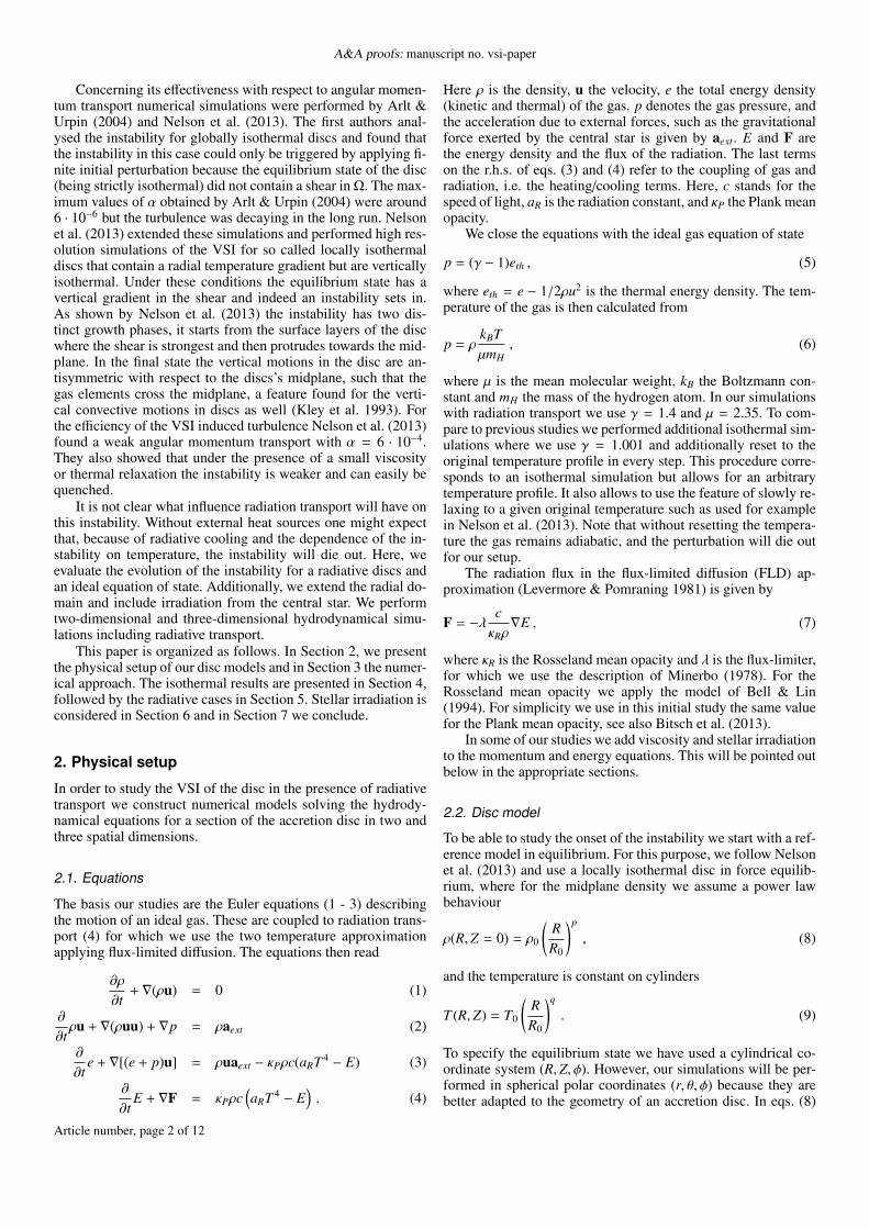
Fig. 1. The kinetic energy of the motion in the meridional plane at differ-ent radii in an inviscid disc. The kinetic energy at the different locationsis in each case averaged over a radial interval with length 0.5AU. Wenote that the unit of time is given in local periods at the center of thespecified interval. Hence, it is different for each curve but this allowsfor easy comparison.

in the meridional plane

ekin =12ρ(u2

r + u2θ) , (14)

at different radii. The obtained growth of ekin of a run withq = −1 and p = −3/2 is displayed at different radii in Fig. 1 foran inviscid disc model with a grid resolution of 2048×512. Notethat the time is measured in local orbits (2π/Ω(ri)) at the corre-sponding centers of the intervals, ri. We measure a mean growthrate of 0.38 per orbit for the kinetic energy (light blue line inFig. 1), which is twice the growth rate (σ) of the velocity. Wecalculate the growth rate by averaging the kinetic energy at thedifferent ri over an interval with length 0.5AU. Our results com-pare favourably with the growth rates from Nelson et al. (2013)who obtained 0.25 per orbit averaged over 1 − 2AU for q = −1.Averaging over this larger range leads to a reduced growth be-cause the rate at 2AU, measured in orbits at 1AU, is smaller by afactor of 21.5 = 2.8, and so their result is a slight underestimate.

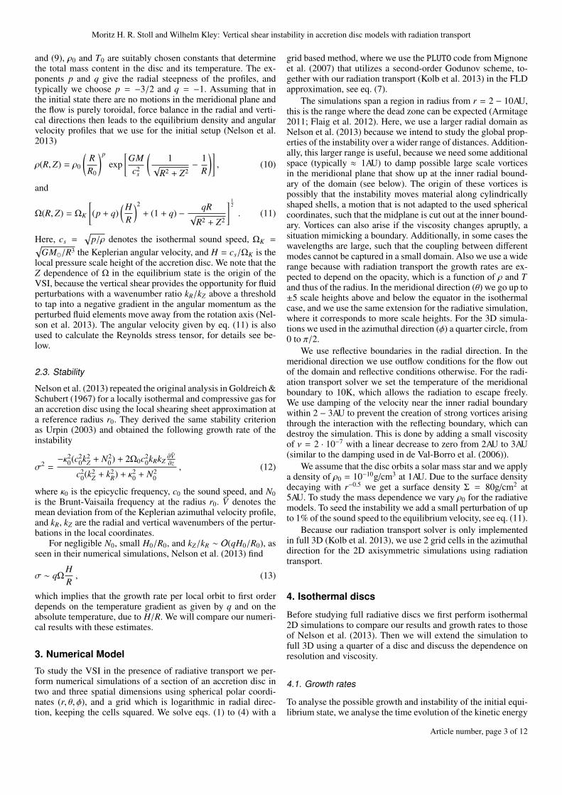
A closer look at figure 1 reveals two distinct growth phases.An initial strong linear growth phase with a rate of 0.38 per orbitlasting about 20 local orbits, and a slower second phase with arate of 0.10 per orbit (gray line in Fig. 1). To understand theseregimes, we present in Fig. 2 the velocity in the meridional di-rection, uθ, in 2D contour plots at different times. The top panelreveals that the first phase corresponds to symmetric (mirrorsymmetry with respect to the equatorial plane) disturbances thatgrow from the top and bottom surface layers of the disc. Here,the gas does not cross the midplane of the disc. When those meetin the disc’s midplane they develop an anti-symmetric phase withlower growth rates where the gas flow crosses the midplane ofthe disc as displayed in the middle panel. The converged phaseshown in the lower panel then shows the fully saturated globalflow. Figure 2 indicates that in the top panel the whole domainis still in the anti-symmetric growth phase, in the middle panelonly the smaller radii show symmetric growth, while in the lowerpanel the whole domain has reached the final equilibrium, in ac-cordance with Fig. 1.

We point out that the growth rate per local orbit (∼ σ/Ω) isindependent of radius in good agreement with the relation (13),for constant H/R. We will show later that the growth rate is alsoindependent of resolution.

Fig. 2. Velocity in the meridional direction, uθ, in units of local Ke-pler velocity for an isothermal run without viscosity. The panels referto snapshots taken at time 100, 210 and 750 (top to bottom), measuredin orbital periods at 1AU. In units of local orbits at (2.5, 3.5, 4.5)AUthis refers to (25, 15, 10) (53, 32, 22) (190, 115, 79) orbits, from top tobottom.

4.2. Comparison to 3D results and Reynolds stress

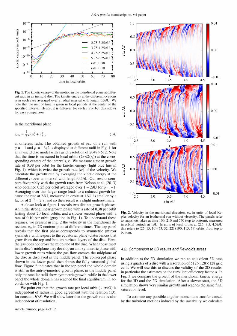
In addition to the 2D simulation we ran an equivalent 3D caseusing a quarter of a disc with a resolution of 512×128×128 gridcells. We will use this to discuss the validity of the 2D results,in particular the estimates on the turbulent efficiency factor α. InFig. 3 we compare the growth of the meridional kinetic energyfor the 3D and the 2D simulation. After a slower start, the 3Dsimulation shows very similar growth and reaches the same finalsaturation level.

To estimate any possible angular momentum transfer causedby the turbulent motions induced by the instability we calculate



0 10 20 30 40 50 60 70 80time in orbits at 4AU

10−12

10−11

10−10

10−9

10−8

10−7

10−6

kine

ticen

ergy

inco

deun

its

quarterdisk2D

Fig. 3. The growth of the kinetic energy for the quarter of a disc and the2D equivalent. The kinetic energy is averaged from 4AU to 5.5AU.

the corresponding Reynolds stress (Balbus 2003)

Trφ =

∫ρδurδuφdV

∆V=< ρδurδuφ > , (15)

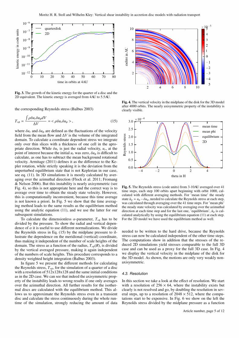
where δur and δuφ are defined as the fluctuations of the velocityfield from the mean flow and ∆V is the volume of the integrateddomain. To calculate a coordinate dependent stress we integrateonly over thin slices with a thickness of one cell in the apro-priate direction. While δur is just the radial velocity, ur, at thepoint of interest because the initial ur was zero, δuφ is difficult tocalculate, as one has to subtract the mean background rotationalvelocity. Armitage (2011) defines it as the difference to the Ke-pler rotation, while strictly speaking it is the deviation from theunperturbed equilibrium state that is not Keplerian in our case,see eq. (11). In 3D simulations it is mostly calculated by aver-aging over the azimuthal direction (Flock et al. 2011; Fromang& Nelson 2006). But this instability is nearly axisymmetric (seeFig. 4), so this is not appropriate here and the correct way is toaverage over time to obtain the steady state velocity. However,this is computationally inconvenient, because this time averageis not known a priori. In Fig. 5 we show that the time averag-ing method leads to the same results as the equilibrium methodusing the analytic equation (11), and we use the latter for oursubsequent simulations.

To calculate the dimensionless α-parameter, Trφ has to bedivided by the pressure. To show the radial and vertical depen-dence of α it is useful to use different normalizations. We dividethe Reynolds stress in Eq. (15) by the midplane pressure to il-lustrate the dependence on the meridional (vertical) coordinate,thus making it independent of the number of scale heights of thedomain. The stress as a function of the radius, Trφ(R), is dividedby the vertical averaged pressure, making it again independentof the numbers of scale heights. This procedure corresponds to adensity weighted height integration (Balbus 2003).

In figure 5 we present the different methods for calculatingthe Reynolds stress, Trφ, for the simulation of a quarter of a discwith a resolution of 512x128x128 and the same initial conditionsas in the 2D case. We can see that indeed the axisymmetric prop-erty of the instability leads to wrong results if one only averagesover the azimuthal direction. All further results for the isother-mal discs are calculated with the equilibrium method. This al-lows us to approximate the Reynolds stress even in a transientdisc and calculate the stress continuously during the whole run-time of the simulation, strongly reducing the amount of data

Fig. 4. The vertical velocity in the midplane of the disk for the 3D modelafter 4000 orbits. The nearly axisymmetric property of the instability isclearly visible.

−4 −2 0 2 4theta in H

0.0

0.5

1.0

1.5

2.0

2.5

3.0R

eyno

lds

stre

ss×10−4

mean timemean phiequilibrium2D

Fig. 5. The Reynolds stress (code units) from 3-10AU averaged over 41time steps, each step 100 orbits apart beginning with orbit 1000, cal-culated with different averaging methods. For ’mean time’ the steadystate uφ = uφ−δuφ, needed to calculate the Reynolds stress at each step,was calculated through averaging over the 41 time steps. For ’mean phi’the steady state velocity was calculated by averaging over the azimuthaldirection at each time step and for the last one, ’equilibrium’, uφ is cal-culated analytically by using the equilibrium equation (11) at each step.For the 2D model we have used the equilibrium method as well.

needed to be written to the hard drive, because the Reynoldsstress can now be calculated independent of the other time steps.The computations show in addition that the stresses of the re-duced 2D simulations yield stresses comparable to the full 3Dcase and can be used as a proxy for the full 3D case. In Fig. 4we display the vertical velocity in the midplane of the disk forthe 3D model. As shown, the motions are only very weakly non-axisymmetric.

4.3. Resolution

In this section we take a look at the effect of resolution. We startwith a resolution of 256 × 64, where the instability exists butclearly is not resolved and go, by doubling the resolution in sev-eral steps, up to a resolution of 2048 × 512, where the compu-tations start to be expensive. In Fig. 6 we show on the left theReynolds stress divided by the midplane pressure as a function



-0.2 -0.1 0.0 0.1 0.2

theta - π/2

10−6

10−5

10−4

Rey

nold

sst

ress

/P0

3 4 5 6 7 8r in AU

0

1

2

3

4

5

6

Rey

nold

sst

ress

/<P>

×10−4

res256res512res1024res2048

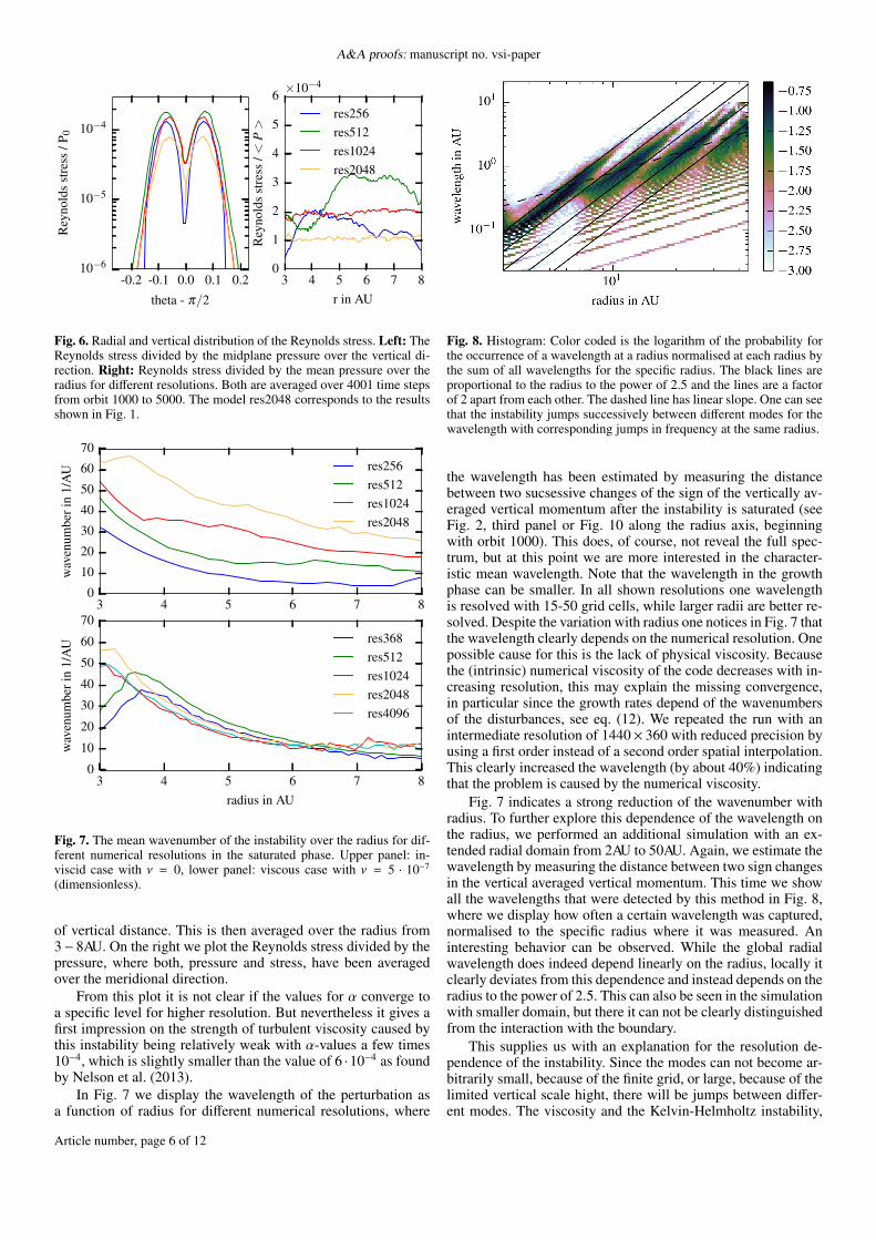
Fig. 6. Radial and vertical distribution of the Reynolds stress. Left: TheReynolds stress divided by the midplane pressure over the vertical di-rection. Right: Reynolds stress divided by the mean pressure over theradius for different resolutions. Both are averaged over 4001 time stepsfrom orbit 1000 to 5000. The model res2048 corresponds to the resultsshown in Fig. 1.

3 4 5 6 7 80

10

20

30

40

50

60

70

wav

enum

beri

n1/

AU res256

res512res1024res2048

3 4 5 6 7 8radius in AU

0

10

20

30

40

50

60

70

wav

enum

beri

n1/

AU res368

res512res1024res2048res4096

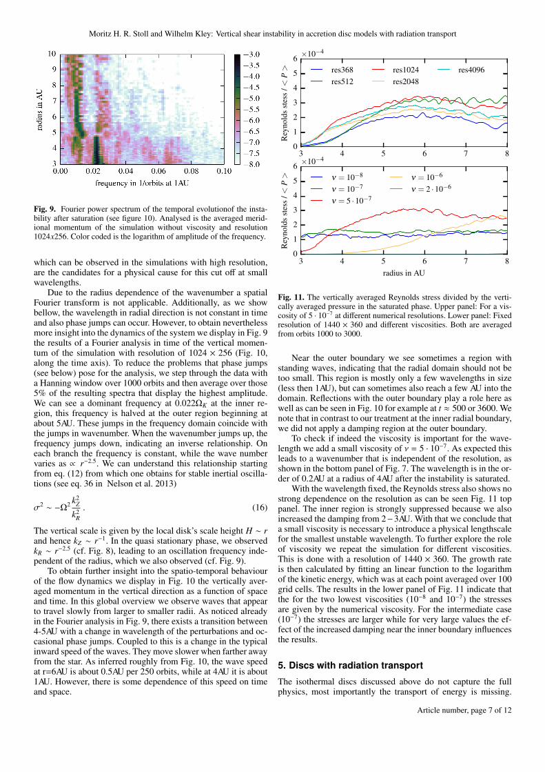
Fig. 7. The mean wavenumber of the instability over the radius for dif-ferent numerical resolutions in the saturated phase. Upper panel: in-viscid case with ν = 0, lower panel: viscous case with ν = 5 · 10−7

(dimensionless).

of vertical distance. This is then averaged over the radius from3− 8AU. On the right we plot the Reynolds stress divided by thepressure, where both, pressure and stress, have been averagedover the meridional direction.

From this plot it is not clear if the values for α converge toa specific level for higher resolution. But nevertheless it gives afirst impression on the strength of turbulent viscosity caused bythis instability being relatively weak with α-values a few times10−4, which is slightly smaller than the value of 6 ·10−4 as foundby Nelson et al. (2013).

In Fig. 7 we display the wavelength of the perturbation asa function of radius for different numerical resolutions, where

Fig. 8. Histogram: Color coded is the logarithm of the probability forthe occurrence of a wavelength at a radius normalised at each radius bythe sum of all wavelengths for the specific radius. The black lines areproportional to the radius to the power of 2.5 and the lines are a factorof 2 apart from each other. The dashed line has linear slope. One can seethat the instability jumps successively between different modes for thewavelength with corresponding jumps in frequency at the same radius.

the wavelength has been estimated by measuring the distancebetween two sucsessive changes of the sign of the vertically av-eraged vertical momentum after the instability is saturated (seeFig. 2, third panel or Fig. 10 along the radius axis, beginningwith orbit 1000). This does, of course, not reveal the full spec-trum, but at this point we are more interested in the character-istic mean wavelength. Note that the wavelength in the growthphase can be smaller. In all shown resolutions one wavelengthis resolved with 15-50 grid cells, while larger radii are better re-solved. Despite the variation with radius one notices in Fig. 7 thatthe wavelength clearly depends on the numerical resolution. Onepossible cause for this is the lack of physical viscosity. Becausethe (intrinsic) numerical viscosity of the code decreases with in-creasing resolution, this may explain the missing convergence,in particular since the growth rates depend of the wavenumbersof the disturbances, see eq. (12). We repeated the run with anintermediate resolution of 1440× 360 with reduced precision byusing a first order instead of a second order spatial interpolation.This clearly increased the wavelength (by about 40%) indicatingthat the problem is caused by the numerical viscosity.

Fig. 7 indicates a strong reduction of the wavenumber withradius. To further explore this dependence of the wavelength onthe radius, we performed an additional simulation with an ex-tended radial domain from 2AU to 50AU. Again, we estimate thewavelength by measuring the distance between two sign changesin the vertical averaged vertical momentum. This time we showall the wavelengths that were detected by this method in Fig. 8,where we display how often a certain wavelength was captured,normalised to the specific radius where it was measured. Aninteresting behavior can be observed. While the global radialwavelength does indeed depend linearly on the radius, locally itclearly deviates from this dependence and instead depends on theradius to the power of 2.5. This can also be seen in the simulationwith smaller domain, but there it can not be clearly distinguishedfrom the interaction with the boundary.

This supplies us with an explanation for the resolution de-pendence of the instability. Since the modes can not become ar-bitrarily small, because of the finite grid, or large, because of thelimited vertical scale hight, there will be jumps between differ-ent modes. The viscosity and the Kelvin-Helmholtz instability,



Fig. 9. Fourier power spectrum of the temporal evolutionof the insta-bility after saturation (see figure 10). Analysed is the averaged merid-ional momentum of the simulation without viscosity and resolution1024x256. Color coded is the logarithm of amplitude of the frequency.

which can be observed in the simulations with high resolution,are the candidates for a physical cause for this cut off at smallwavelengths.

Due to the radius dependence of the wavenumber a spatialFourier transform is not applicable. Additionally, as we showbellow, the wavelength in radial direction is not constant in timeand also phase jumps can occur. However, to obtain neverthelessmore insight into the dynamics of the system we display in Fig. 9the results of a Fourier analysis in time of the vertical momen-tum of the simulation with resolution of 1024 × 256 (Fig. 10,along the time axis). To reduce the problems that phase jumps(see below) pose for the analysis, we step through the data witha Hanning window over 1000 orbits and then average over those5% of the resulting spectra that display the highest amplitude.We can see a dominant frequency at 0.022ΩK at the inner re-gion, this frequency is halved at the outer region beginning atabout 5AU. These jumps in the frequency domain coincide withthe jumps in wavenumber. When the wavenumber jumps up, thefrequency jumps down, indicating an inverse relationship. Oneach branch the frequency is constant, while the wave numbervaries as ∝ r−2.5. We can understand this relationship startingfrom eq. (12) from which one obtains for stable inertial oscilla-tions (see eq. 36 in Nelson et al. 2013)

σ2 ∼ −Ω2 k2Z

k2R

. (16)

The vertical scale is given by the local disk’s scale height H ∼ rand hence kZ ∼ r−1. In the quasi stationary phase, we observedkR ∼ r−2.5 (cf. Fig. 8), leading to an oscillation frequency inde-pendent of the radius, which we also observed (cf. Fig. 9).

To obtain further insight into the spatio-temporal behaviourof the flow dynamics we display in Fig. 10 the vertically aver-aged momentum in the vertical direction as a function of spaceand time. In this global overview we observe waves that appearto travel slowly from larger to smaller radii. As noticed alreadyin the Fourier analysis in Fig. 9, there exists a transition between4-5AU with a change in wavelength of the perturbations and oc-casional phase jumps. Coupled to this is a change in the typicalinward speed of the waves. They move slower when farther awayfrom the star. As inferred roughly from Fig. 10, the wave speedat r=6AU is about 0.5AU per 250 orbits, while at 4AU it is about1AU. However, there is some dependence of this speed on timeand space.

3 4 5 6 7 80

1

2

3

4

5

6

Rey

nold

sst

ess

/<P>

×10−4

res368res512

res1024res2048

res4096


0

1

2

3

4

5

6

Rey

nold

sst

ess

/<P>

×10−4

ν = 10−8

ν = 10−7

ν = 5 ·10−7

ν = 10−6

ν = 2 ·10−6

Fig. 11. The vertically averaged Reynolds stress divided by the verti-cally averaged pressure in the saturated phase. Upper panel: For a vis-cosity of 5 · 10−7 at different numerical resolutions. Lower panel: Fixedresolution of 1440 × 360 and different viscosities. Both are averagedfrom orbits 1000 to 3000.

Near the outer boundary we see sometimes a region withstanding waves, indicating that the radial domain should not betoo small. This region is mostly only a few wavelengths in size(less then 1AU), but can sometimes also reach a few AU into thedomain. Reflections with the outer boundary play a role here aswell as can be seen in Fig. 10 for example at t ≈ 500 or 3600. Wenote that in contrast to our treatment at the inner radial boundary,we did not apply a damping region at the outer boundary.

To check if indeed the viscosity is important for the wave-length we add a small viscosity of ν = 5 · 10−7. As expected thisleads to a wavenumber that is independent of the resolution, asshown in the bottom panel of Fig. 7. The wavelength is in the or-der of 0.2AU at a radius of 4AU after the instability is saturated.

With the wavelength fixed, the Reynolds stress also shows nostrong dependence on the resolution as can be seen Fig. 11 toppanel. The inner region is strongly suppressed because we alsoincreased the damping from 2−3AU. With that we conclude thata small viscosity is necessary to introduce a physical lengthscalefor the smallest unstable wavelength. To further explore the roleof viscosity we repeat the simulation for different viscosities.This is done with a resolution of 1440 × 360. The growth rateis then calculated by fitting an linear function to the logarithmof the kinetic energy, which was at each point averaged over 100grid cells. The results in the lower panel of Fig. 11 indicate thatthe for the two lowest viscosities (10−8 and 10−7) the stressesare given by the numerical viscosity. For the intermediate case(10−7) the stresses are larger while for very large values the ef-fect of the increased damping near the inner boundary influencesthe results.

5. Discs with radiation transport

The isothermal discs discussed above do not capture the fullphysics, most importantly the transport of energy is missing.



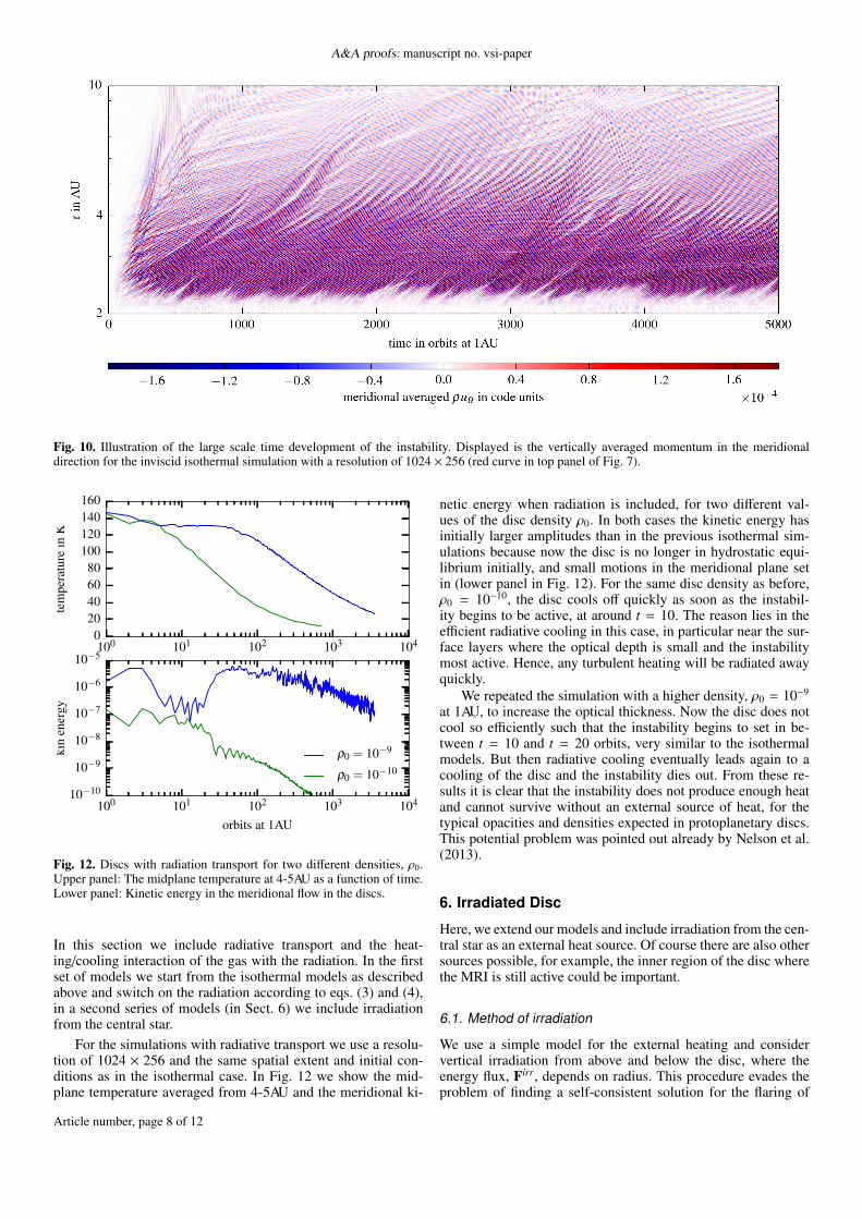
Fig. 10. Illustration of the large scale time development of the instability. Displayed is the vertically averaged momentum in the meridionaldirection for the inviscid isothermal simulation with a resolution of 1024 × 256 (red curve in top panel of Fig. 7).

100 101 102 103 1040

20406080

100120140160

tem

pera

ture

inK

100 101 102 103 104

orbits at 1AU

10−10

10−9

10−8

10−7

10−6

10−5

kin

ener

gy

ρ0 = 10−9

ρ0 = 10−10

Fig. 12. Discs with radiation transport for two different densities, ρ0.Upper panel: The midplane temperature at 4-5AU as a function of time.Lower panel: Kinetic energy in the meridional flow in the discs.

In this section we include radiative transport and the heat-ing/cooling interaction of the gas with the radiation. In the firstset of models we start from the isothermal models as describedabove and switch on the radiation according to eqs. (3) and (4),in a second series of models (in Sect. 6) we include irradiationfrom the central star.

For the simulations with radiative transport we use a resolu-tion of 1024 × 256 and the same spatial extent and initial con-ditions as in the isothermal case. In Fig. 12 we show the mid-plane temperature averaged from 4-5AU and the meridional ki-

netic energy when radiation is included, for two different val-ues of the disc density ρ0. In both cases the kinetic energy hasinitially larger amplitudes than in the previous isothermal sim-ulations because now the disc is no longer in hydrostatic equi-librium initially, and small motions in the meridional plane setin (lower panel in Fig. 12). For the same disc density as before,ρ0 = 10−10, the disc cools off quickly as soon as the instabil-ity begins to be active, at around t = 10. The reason lies in theefficient radiative cooling in this case, in particular near the sur-face layers where the optical depth is small and the instabilitymost active. Hence, any turbulent heating will be radiated awayquickly.

We repeated the simulation with a higher density, ρ0 = 10−9

at 1AU, to increase the optical thickness. Now the disc does notcool so efficiently such that the instability begins to set in be-tween t = 10 and t = 20 orbits, very similar to the isothermalmodels. But then radiative cooling eventually leads again to acooling of the disc and the instability dies out. From these re-sults it is clear that the instability does not produce enough heatand cannot survive without an external source of heat, for thetypical opacities and densities expected in protoplanetary discs.This potential problem was pointed out already by Nelson et al.(2013).

6. Irradiated Disc

Here, we extend our models and include irradiation from the cen-tral star as an external heat source. Of course there are also othersources possible, for example, the inner region of the disc wherethe MRI is still active could be important.

6.1. Method of irradiation

We use a simple model for the external heating and considervertical irradiation from above and below the disc, where theenergy flux, Firr, depends on radius. This procedure evades theproblem of finding a self-consistent solution for the flaring of



3.0 3.5 4.0 4.5 5.0 5.5 6.0 6.5 7.0radius in AU

0.0

0.1

0.2

0.3

0.4

0.5

0.6

0.7

grow

thra

tein

Ω

iso2048 ν = 10−7

iso1024 ν = 0irr2048 ν = 10−7

irr1024 ν = 0

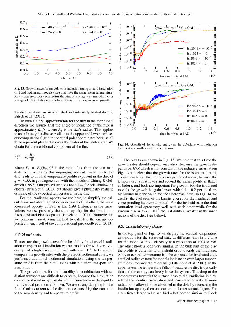
Fig. 13. Growth rates for models with radiation transport and irradiation(irr) and isothermal models (iso) that have the same mean temperature,for comparison. For each radius the kinetic energy was smoothed overa range of 10% of its radius before fitting it to an exponential growth.

the disc, as done for an irradiated and internally heated disc byBitsch et al. (2013).

To obtain a first approximation for the flux in the meridionaldirection we assume that the angle of incidence of the flux isapproximately R/r, where R is the star’s radius. This appliesto an infinitely flat disc as well as to the upper and lower surfacesour computational grid in spherical polar coordinates because allthree represent planes that cross the center of the central star. Weobtain for the meridional component of the flux

F irrθ = Fr

RR, (17)

where Fr = F(R/r)2 is the radial flux from the star at adistance r. Applying this impinging vertical irradiation to thedisc leads to a radial temperature profile exponent in the disc ofq = −0.55, in good agreement with the models of Chiang & Gol-dreich (1997). Our procedure does not allow for self-shadowingeffects (Bitsch et al. 2013) but should give a physically realisticestimate of the expected temperatures in the disc.

For the irradiation opacity we use here, to simplify the cal-culations and obtain a first order estimate of the effect, the sameRosseland opacity of Bell & Lin (1994). Hence, in the simu-lations we use presently the same opacity for the irradiation,Rosseland and Planck opacity (Bitsch et al. 2013). Numerically,we perform a ray-tracing method to calculate the energy de-posited in each cell of the computational grid (Kolb et al. 2013).

6.2. Growth rate

To measure the growth rates of the instability for discs with radi-ation transport and irradiation we ran models for with zero vis-cosity and a higher resolution case with ν = 10−7. To be able tocompare the growth rates with the previous isothermal cases, weperformed additional isothermal simulations using the temper-ature profile from the simulations with radiation transport andirradiation.

The growth rates for the instability in combination with ra-diation transport are difficult to capture, because the simulationcan not be started in hydrostatic equilibrium because the equilib-rium vertical profile is unknown. We use strong damping for thefirst 10 orbits to remove the disturbance caused by the transitionto the new density and temperature profile.

0.0 0.2 0.4 0.6 0.8 1.0 1.2 1.4time in orbits at 1AU ×103

10−13

10−12

10−11

10−10

10−9

10−8

10−7

mea

nki

netic

ener

gyin

code

units

growth rates at 3.0-4.0AU

iso2048 ν = 10−7

iso1024 ν = 0irr2048 ν = 10−7

irr1024 ν = 0

0.0 0.2 0.4 0.6 0.8 1.0 1.2 1.4time in orbits at 1AU ×103

10−13

10−12

10−11

10−10

10−9

10−8

10−7

mea

nki

netic

ener

gyin

code

units

growth rates at 5.0-8.0AU

iso2048 ν = 10−7

iso1024 ν = 0irr2048 ν = 10−7

irr1024 ν = 0

Fig. 14. Growth of the kinetic energy in the 2D-plane with radiationtransport and isothermal for comparison.

The results are shown in Fig. 13. We note that this time thegrowth rates should depend on radius, because the growth de-pends on H/R which is not constant in the radiative cases. FromFig. 13 it is clear that the growth rates for the isothermal mod-els are now lower than in the cases presented above, because thetemperature is first lower and second the radial profile is flatteras before, and both are important for growth. For the irradiatedmodels the growth is again lower, with 0.1 − 0.2 per local or-bit around half the value for the isothermal case. In Fig. 14 wedisplay the evolution of the kinetic energy for the irradiated andcorresponding isothermal model. For the inviscid case the finalsaturation level agree very well with each other while for theviscous disc with ν = 10−7 the instability is weaker in the innerregions of the disc (see below).

6.3. Quasistationary phase

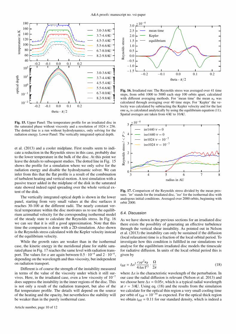
In the top panel of Fig. 15 we display the vertical temperaturedistribution for the saturated state at different radii in the discfor the model without viscosity at a resolution of 1024 × 256.The other models look very similar. In the bulk part of the discthe profile is quite flat with a slight drop towards the midplane.A lower central temperature is to be expected for irradiated dics,detailed radiative transfer models indicate an even larger temper-ature drop towards the midplane (Dullemond et al. 2002). In theupper layers the temperature falls off because the disc is opticallythin and the energy can freely leave the system. This drop of thetemperatures towards the surface despite the irradiation is a re-sult of the identical irradiation and Rosseland opacity. If moreradiation is allowed to be absorbed in the disk by increasing theirradiation opacity then one can obtain hotter surface layers. Fora ten times larger value we find a hot corona similar to Flock



-0.2 -0.1 0.0 0.1 0.2

theta - π/2

10−2

10−1

100

101

102

optic

alde

pth

3.0-3.6AU3.7-4.4AU4.5-5.4AU5.5-6.6AU6.7-8.0AU8.2-9.8AU

-0.2 -0.1 0.0 0.1 0.2406080

100120140160180

tem

pera

ture

inK 3.0-3.6AU

3.7-4.4AU4.5-5.4AU5.5-6.6AU6.7-8.0AU8.2-9.8AU

Fig. 15. Upper Panel: The temperature profile for an irradiated disc inthe saturated phase without viscosity and a resolution of 1024 × 256.The dotted line is a run without hydrodynamics, only solving for theradiation energy. Lower Panel: The vertically integrated optical depth.

et al. (2013) and a cooler midplane. First results seem to indi-cate a reduction in the Reynolds stress in this case, probably dueto the lower temperature in the bulk of the disc. At this point weleave the details to subsequent studies. The dotted line in Fig. 15shows the profile for a simulation where we only solve for theradiation energy and disable the hydrodynamic solver. We caninfer from this that the flat profile is a result of the combinationof turbulent heating and vertical motion. A test simulation with apassive tracer added in the midplane of the disk in the saturatedstate showed indeed rapid spreading over the whole vertical ex-tent of the disk.

The vertically integrated optical depth is shown in the lowerpanel, starting from very small values at the disc surfaces itreaches 30-100 at the different radii. The nearly constant ver-tical temperature within the disc motivates us to use the equilib-rium azimuthal velocity for the corresponding isothermal modelof the steady state to calculate the Reynolds stress. In Fig. 16we can see that it is still a good approximation. Note that thistime the comparison is done with a 2D-simulation. Also shownis the Reynolds stress calculated with the Kepler velocity insteadof the equilibrium velocity.

While the growth rates are weaker than in the isothermalcase, the kinetic energy in the meridional plane for stable satu-rated phase in Fig. 17 reaches the same level with radiation trans-port. The values for α are again between 0.5 · 10−4 and 2 · 10−4,depending on the wavelength and thus viscosity, but independenton radiation transport.

Different is of course the strength of the instability measuredin terms of the value of the viscosity under which it still sur-vives. Here, in the irradiated case, even a low viscosity of 10−7

does suppress the instability in the inner regions of the disc. Thisis not only a result of the radiation transport, but also of theflat temperature profile. The details will depend on the sourceof the heating and the opacity, but nevertheless the stability willbe weaker than in the purely isothermal case.

−0.2 −0.1 0.0 0.1 0.2

theta - π/2

−1.5−1.0−0.5

0.00.51.01.52.02.53.0

Rey

nold

sst

ress

×10−4

mean timeKeplerequilibrium

Fig. 16. Irradiated run: The Reynolds stress was averaged over 41 timesteps, from orbit 1000 to 5000 each step 100 orbits apart, calculatedwith different averaging methods. For ’mean time’ the mean uφ wascalculated through averaging over 40 time steps. For ’Kepler’ the ve-locity was calculated by subtracting the Kepler velocity and for the lastone uφ is calculated analytically by using the equilibrium equation (11).Spatial averages are taken from 4AU to 10AU.


0

1

2

3

4

5R

eyno

lds

stre

ss/<

P>

×10−4

irr1440 ν = 0iso1440 ν = 0irr1024 ν = 10−7

iso1024 ν = 10−7

Fig. 17. Comparison of the Reynolds stress divided by the mean pres-sure. ’irr’ stands for the irradiated disc, ’iso’ for the isothermal disc withanalogous initial conditions. Averaged over 2000 orbits, beginning withorbit 2000.

6.4. Discussion

As we have shown in the previous sections for an irradiated discthere exists the possiblity of generating an effective turbulencethrough the vertical shear instability. As pointed out in Nelsonet al. (2013) the instability can only be sustained if the diffusion(local relaxation) time is a fraction of the local orbital period. Toinvestigate how this condition is fulfilled in our simulations weanalyse for the equilibrium irradiated disc models the timescalefor radiative diffusion. In units of the local orbital period this isgiven by

tdiff = ∆x2 cPρ2κR

4λacT 3 ·Ω

2π(18)

where ∆x is the characteristic wavelength of the perturbation. Inour case the radial diffusion is relevant (Nelson et al. 2013) andwe choose here ∆x = 0.05r, which is a typical radial wavelengthat r = 3AU. Using eq. (18) and the results from the simulationwe calculate for the optical thin region a very small cooling timeper orbit of tdiff = 10−10 as expected. For the optical thick regionwe obtain tdiff = 0.11 for our standard density, which is indeed a



-0.2 -0.1 0.0 0.1 0.2

theta - π/2

10−1310−1210−1110−1010−910−810−710−610−510−410−310−210−1

100101

cool

ing

time

pero

rbit

irr res2048, ρ0

irr res2048, 2 ·ρ0

irr res2048, 5 ·ρ0

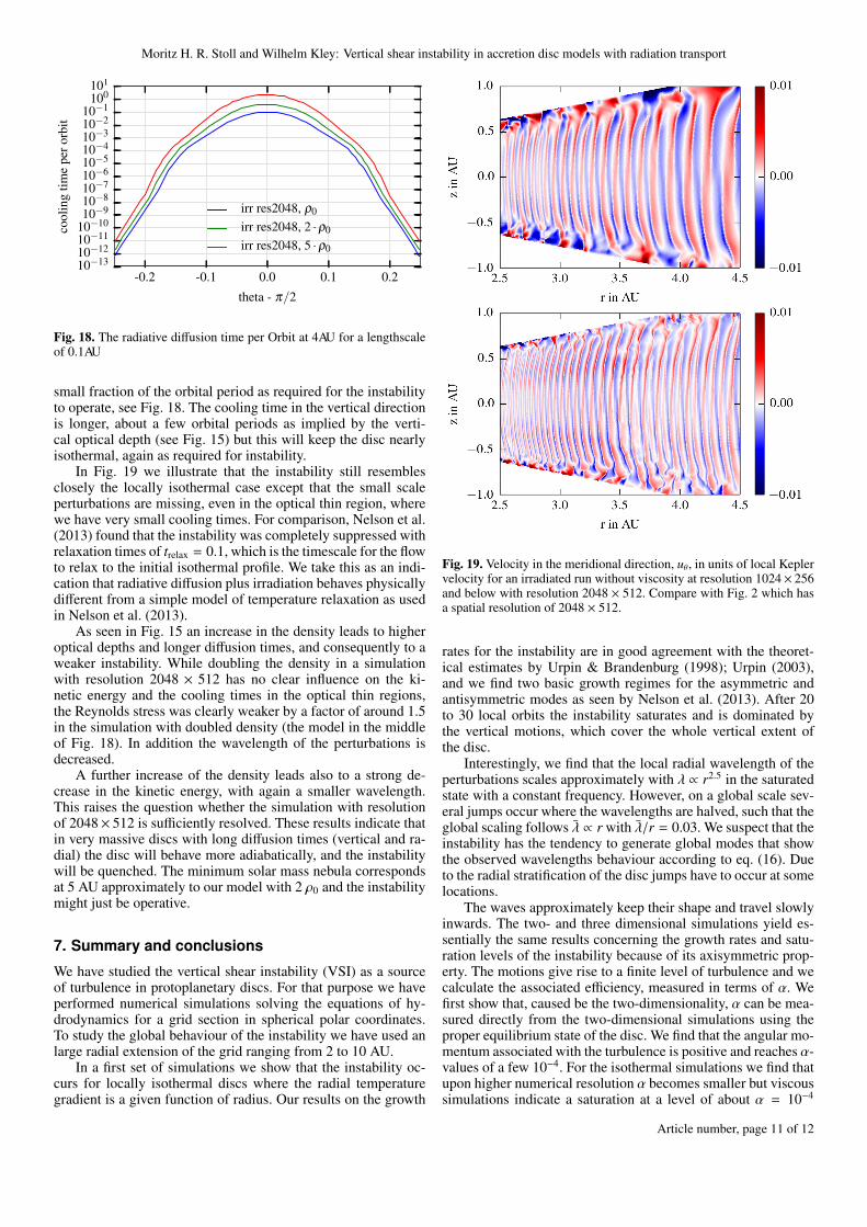
Fig. 18. The radiative diffusion time per Orbit at 4AU for a lengthscaleof 0.1AU

small fraction of the orbital period as required for the instabilityto operate, see Fig. 18. The cooling time in the vertical directionis longer, about a few orbital periods as implied by the verti-cal optical depth (see Fig. 15) but this will keep the disc nearlyisothermal, again as required for instability.

In Fig. 19 we illustrate that the instability still resemblesclosely the locally isothermal case except that the small scaleperturbations are missing, even in the optical thin region, wherewe have very small cooling times. For comparison, Nelson et al.(2013) found that the instability was completely suppressed withrelaxation times of trelax = 0.1, which is the timescale for the flowto relax to the initial isothermal profile. We take this as an indi-cation that radiative diffusion plus irradiation behaves physicallydifferent from a simple model of temperature relaxation as usedin Nelson et al. (2013).

As seen in Fig. 15 an increase in the density leads to higheroptical depths and longer diffusion times, and consequently to aweaker instability. While doubling the density in a simulationwith resolution 2048 × 512 has no clear influence on the ki-netic energy and the cooling times in the optical thin regions,the Reynolds stress was clearly weaker by a factor of around 1.5in the simulation with doubled density (the model in the middleof Fig. 18). In addition the wavelength of the perturbations isdecreased.

A further increase of the density leads also to a strong de-crease in the kinetic energy, with again a smaller wavelength.This raises the question whether the simulation with resolutionof 2048× 512 is sufficiently resolved. These results indicate thatin very massive discs with long diffusion times (vertical and ra-dial) the disc will behave more adiabatically, and the instabilitywill be quenched. The minimum solar mass nebula correspondsat 5 AU approximately to our model with 2 ρ0 and the instabilitymight just be operative.

7. Summary and conclusions

We have studied the vertical shear instability (VSI) as a sourceof turbulence in protoplanetary discs. For that purpose we haveperformed numerical simulations solving the equations of hy-drodynamics for a grid section in spherical polar coordinates.To study the global behaviour of the instability we have used anlarge radial extension of the grid ranging from 2 to 10 AU.

In a first set of simulations we show that the instability oc-curs for locally isothermal discs where the radial temperaturegradient is a given function of radius. Our results on the growth

Fig. 19. Velocity in the meridional direction, uθ, in units of local Keplervelocity for an irradiated run without viscosity at resolution 1024× 256and below with resolution 2048 × 512. Compare with Fig. 2 which hasa spatial resolution of 2048 × 512.

rates for the instability are in good agreement with the theoret-ical estimates by Urpin & Brandenburg (1998); Urpin (2003),and we find two basic growth regimes for the asymmetric andantisymmetric modes as seen by Nelson et al. (2013). After 20to 30 local orbits the instability saturates and is dominated bythe vertical motions, which cover the whole vertical extent ofthe disc.

Interestingly, we find that the local radial wavelength of theperturbations scales approximately with λ ∝ r2.5 in the saturatedstate with a constant frequency. However, on a global scale sev-eral jumps occur where the wavelengths are halved, such that theglobal scaling follows λ ∝ r with λ/r = 0.03. We suspect that theinstability has the tendency to generate global modes that showthe observed wavelengths behaviour according to eq. (16). Dueto the radial stratification of the disc jumps have to occur at somelocations.

The waves approximately keep their shape and travel slowlyinwards. The two- and three dimensional simulations yield es-sentially the same results concerning the growth rates and satu-ration levels of the instability because of its axisymmetric prop-erty. The motions give rise to a finite level of turbulence and wecalculate the associated efficiency, measured in terms of α. Wefirst show that, caused be the two-dimensionality, α can be mea-sured directly from the two-dimensional simulations using theproper equilibrium state of the disc. We find that the angular mo-mentum associated with the turbulence is positive and reaches α-values of a few 10−4. For the isothermal simulations we find thatupon higher numerical resolution α becomes smaller but viscoussimulations indicate a saturation at a level of about α = 10−4



even for very small underlying viscosities that are equivalent toα < 10−6.

Adding radiative transport leads to a cooling from the discsurfaces and the instability dies out subsequently. We then con-structed models where the disc is irradiated from above and be-low which leads to a nearly constant vertical temperature profilewithin the disc. This leads again to a turbulent saturated statewith a similar transport efficiency as the purely isothermal sim-ulations, possibly slightly higher (see Fig. 17).

In summary, our simulations indicate that the VSI can indeedgenerate turbulence in discs albeit at a relatively low level ofabout few times 10−4. This implies that even in (magnetically)dead zones the effective viscosity in discs will never fall belowthis level. Our results indicate that in fully 3D simulations thetransport may be marginally larger, but further simulations willhave to be performed to clarify this point.Acknowledgements. Moritz Stoll received financial support from the Landes-graduiertenförderung of the state of Baden-Württemberg. Wilhelm Kley ac-knowledges the support of the German Research Foundation (DFG) throughgrant KL 650/8-2 within the Collaborative Research Group FOR 759: The for-mation of Planets: The Critical First Growth Phase. Some simulations were per-formed on the bwGRiD cluster in Tübingen, which is funded by the Ministry forEducation and Research of Germany and the Ministry for Science, Research andArts of the state Baden-Württemberg, and the cluster of the Forschergruppe FOR759 “The Formation of Planets: The Critical First Growth Phase” funded by theDFG.

ReferencesArlt, R. & Urpin, V. 2004, A&A, 426, 755Armitage, P. J. 2011, ARA&A, 49, 195Balbus, S. A. 2003, ARA&A, 41, 555Bell, K. R. & Lin, D. N. C. 1994, ApJ, 427, 987Bitsch, B., Crida, A., Morbidelli, A., Kley, W., & Dobbs-Dixon, I. 2013, A&A,

549, A124Chiang, E. I. & Goldreich, P. 1997, ApJ, 490, 368de Val-Borro, M., Edgar, R. G., Artymowicz, P., et al. 2006, MNRAS, 370, 529Dullemond, C. P., van Zadelhoff, G. J., & Natta, A. 2002, A&A, 389, 464Flaig, M., Ruoff, P., Kley, W., & Kissmann, R. 2012, MNRAS, 420, 2419Flock, M., Dzyurkevich, N., Klahr, H., Turner, N. J., & Henning, T. 2011, ApJ,

735, 122Flock, M., Fromang, S., González, M., & Commerçon, B. 2013, A&A, 560, A43Fricke, K. 1968, ZAp, 68, 317Fromang, S. & Nelson, R. P. 2006, A&A, 457, 343Goldreich, P. & Schubert, G. 1967, ApJ, 150, 571Klahr, H. H. & Bodenheimer, P. 2003, ApJ, 582, 869Kley, W., Papaloizou, J. C. B., & Lin, D. N. C. 1993, ApJ, 416, 679Kolb, S. M., Stute, M., Kley, W., & Mignone, A. 2013, A&A, 559, A80Levermore, C. D. & Pomraning, G. C. 1981, ApJ, 248, 321Lin, D. N. C. & Pringle, J. E. 1987, MNRAS, 225, 607Mignone, A., Bodo, G., Massaglia, S., et al. 2007, ApJS, 170, 228Minerbo, G. N. 1978, J. Quant. Spec. Radiat. Transf., 20, 541Nelson, R. P., Gressel, O., & Umurhan, O. M. 2013, MNRAS, 435, 2610Pringle, J. E. 1981, ARA&A, 19, 137Ruden, S. P., Papaloizou, J. C. B., & Lin, D. N. C. 1988, ApJ, 329, 739Shakura, N. & Sunyaev, R. 1973, A&A, 24, 337Turner, N. J., Fromang, S., Gammie, C., et al. 2014, ArXiv e-printsUrpin, V. 2003, A&A, 404, 397Urpin, V. & Brandenburg, A. 1998, MNRAS, 294, 399


Documents

Vertical shear instability in accretion disc models with ... · Astronomy & Astrophysics manuscript no. vsi-paper c ESO 2014 October 1, 2014 Vertical shear instability in accretion